
Submitted:
30 April 2025
Posted:
06 May 2025
You are already at the latest version
Abstract
123 mobile phones in the 1.5 GHz-2.1 GHz frequency band are observed for electromagnetic radiation at two distances from the device (0m and 1m) and four distinct ways of usage. Electric field spectra are measured within a seven minute interval. Spectrum measurements minimum, aveage and maximum electric field (Emin,Eave,Emax) are reported.These values range from 0,021 V/m to 15,0 V/m.The Emax spectra peaks are non-systematic,depend on the provider and phone and range between 1,72 GHz and 1,97 GHz. The Emax measurements are compared via box and whiskers plots.The boxplot Q1-Q3 spectra measurements are compared via ANOVA.The measurements between Q1(25%) and Q3 (75 %) quartiles follow the normal distribution while the outliers are more, denser and with higher maximum Emax values at 0m distance (contact with ear) than at 1m away. Through reorganisation of the whole dataset in columns, the four usage ways are compared.Most significant is the usage way of making a call where only the corresponding columns follow the normal distribution.Making a call signifies the emitted electric field.

Keywords:
electromagnetic radiation
; mobile phone
; use
1. Introduction
Due to the ongoing demand for quality, speed and wide application range of modern mobile phones, the wireless technologies have significantly advanced [1]. This is a continuous process that began in the late nineties and is strongly related to the extensive installation of base stations [2]. Due to the development of communication protocols for mobile phone devices, the cellular network providers have constructed network infrastructures over a wide range of frequency bands referenced collectively as 2G, 3G, 4G, and 5G communications. Despite that 5G is regarded as a faster and more secure technology than the previous communication technology systems, the new 5G technology is very new [3] and the suggested frequency range from 24 to 60 ( electromagnetic waves) has not developed all its full potential because the corresponding base stations have not been extensively constructed yet. Due to its very recent development, 5G technology makes advantage of recently opened frequencies or frequencies already assigned to 3G or 4G [3]. Especially in Greece even the specific 5G frequency range between 24.25 and 29.5 have not be developed satisfactory yet. Despite 5G allows for antenna array technologies of improved directivity, reduced latency and increased data transmission speeds [3], the 3G and 4G frequency band technologies are still dominant in Greece and this despite the fact that the network providers indicate 5G technology in the mobile smartphone devices. Mobile phones have undergone a remarkable rise in use over the past twenty years with over 80% of people owning and using mobile phone devices [4]. It is nearly hard to imagine a world without smartphones given how commonplace such devices have become in the everyday life [5]. A primary factor that boosts this growing trend, is the extensive internet access and the applications that are nowadays available by all cellular network providers [6]. Despite however the widespread usage of mobile phones, there is a growing unawareness of the hazards associated with the exposure to radiofrequency (RF) electromagnetic fields (EMF) [7]. This gives rise to concerns over the possible health consequences that result from extended exposure to radiofrequency radiation emanating from mobile devices [e.g [8,9,10,11]. The problem however, is restricted not only to mobile phones and the corresponding 2G-5G frequency range, but rather extends to the effects due to various sources and a wide range of frequency bands. Due to the international interest on the health effects of the electromagnetic fields, reputed worldwide organisations, such as the International Commission on Non-Ionizing Radiation Protection and the International Committee on Electromagnetic Safety of the Institute of Electrical and Electronics Engineers (IEEE) have issued guidelines [7,12,13,14] which address the potential health risks due to the exposure of the general population to electromagnetic fields, as well as related safety precautions [15]. The ICNIRP’s guidelines are not regulatory. They rather set scientifically justified standards and a set of basic restrictions and reference levels [15]. The legislative organisation for Greece is European Union. European Union’s legal area is strict and challenging, but the regulatory limits of 2010 [16] are based on the 2010 ICNIRP’s report [12] and those of 1998 [17], to the 1998 ICNIRP’s report [13]. Only some updates of technical standards refer to the current ICNIRP’s 2020 guidelines [7]. The cellular network in Greece by far cannot be characterised as structured. In the last twenty years, the cellular network providers have changed names and ownership twice. Companies with many subscribers do not exist any more, while nowadays, three main providers have the majority of subscribers. In the last five years some fibre optics television providers try to get into the optical telephony and the mobile phone activity. The Hellenic state did not manage to control this boost. As a result, telecommunications antennas and receivers in big cities like Athens, have been installed without specific control and the same is the case for the cellular receivers and emitters. Several cellular type antennas are hidden in places that cannot be easily traced, such as billboards, tablets and signs. Any attempt from the state to rationalise this situation has not yet paid off. As a result the exposure of the Greek population to RF EMF from mobile phones is not known, neither the effects of the different usage scenarios of the mobile phones. The responsible Greek authority is the Hellenic Committee on Radiation Protection with offices within the Demokritos research centre of Greece, in Athens. This Committee may conduct checks by order of another authority or institution. Therefore, the research on mobile phone usage in Greece and, especially, Athens is limited. Hence there is a scientific gap which, importantly, is not of local character. Indeed, the papers of the last years focus on the negative effects of driving and using phone [18,19], the use of GPS smartphone data to achieve certain actions [20], in urban sensing [21], in mobile security [22], the use among pupils [23], students [24] and older people [25], the impact of mobile phone technology on humans [26] and crime applications [27] and various mobile applications development. Contemporary papers on the effects of mobile phone radiation focus on base stations [28] and on human head models [29]. Although the aim of this paper is not to provide a comprehensive review of the subject, it becomes evident from the above that there is restricted focus on the different scenarios of the usage of mobile phones and the corresponding effects. In view of the international interest on the potential negative health consequences of radiofrequency electromagnetic fields, this paper reports electric field spectrum measurements for mobile phones operating in Athens Greece in contract with the main cellular providers of Greece. The electric field measurements are conducted with the Narda SRM-3006 instrument for four distinct ways of usage and for two different distances at 0 m and 1 m from the mobile phone. The dataset comprises eighty two mobile different phones from various vendors and cellular network providers of Greece (three total). The aim is to provide a scientific basis for further investigation of the effects that the the phone usage has on the emitted electromagnetic radiation in the nearby environment and also a foundation for more comprehensive EMF measurements, especially in Greece. In the following, the usage ways, the methodology for the electric field measurements and the statistical analysis of the research are described in Section 2. Selected spectrum electric field measurements together with the results from the statistical analysis and the discussion are given in Section 3. The conclusions of the study are presented in Section 4 and the evaluation and the limitations are given in Section 5.
2. Materials and Methods
The employed Narda SRM-3006 instrument for electric field measurements, receives and records electric field spectra, namely, electric field () versus frequency () within a user-defined frequency range and time interval. Minimum (), average () and maximum () electric field values are provided for every frequency bin throughout the duration of each measurement set. In compliance to the ICNIRP and EU recommendations the measurements duration is fixed to seven minutes compensating accuracy in measurement and convenience in recording. Taking into account that 5G is not practically in operation in Greece, the frequency range is set between 1.5 and 2.1 focusing hence on the 4G part of the future 5G network. The investigated ways of usage are given in Table 1.
The electric field spectrum measurements are repeated for every way and mobile phone at 0 m (in contact with the phone) and at 1 m (away from the mobile phone). For each spectrum measurement Narda SMR-3006 is placed on a horizontal wooden table and the mobile phone on a base so as the centre of the telephone’s antenna to be as closely aligned to the centre of the isotropic antenna of Narda SRM-3006,namely the centre of the three passive dipoles of the isotropic antenna that are perpendicular to each other.Narda SMR-3006 is adjusted to start and end at predefined time instances and to collect the electric spectra within these. As mentioned, the predefined measurement interval is seven minutes. During each measurement the experimenter is at least at 3 m away from the measurement setup to minimise bias. The mobile phone is operated via a hands free headphone.
The measurement dataset contain the following categories
- 1.
- Four (4) usage modes;
- 2.
- Two (2) different distances for each mobile phone;
combined with :
Eighty two (82) different mobile phones, namely phones from 82 different vendors, namely 82 electric field spectra from completely different phones;
Some mobile phones are from the same vendor but from a different provider. As a result the total measurements contain:
- (a)
- Two hundred forty six (246) total electric field spectra from mobile phones;
- (b)
- One hundred twenty three (123=246:2) total electric field spectra at 0 m and another one hundred twenty three (123) at 1 m from the source.
The research questions are the following:
- (a)
- Is there any difference in , and between the phones?
- (b)
- What are the differentiations in electric field when using a mobile phone at 0 m and 1 m distance from the source?
- (c)
- Which way of usage is most significant?
Statistical analysis performed in terms of box and whiskers plots, Analysis of Variance (ANOVA), Wilcoxon signed-rank test,t-test and paired t-test.
3. Results and Discussion
Noteworthy variations are found in the electric field spectra. All types of measurements, i.e., , and fluctuate with frequency f in all ways of usage (Table 1). Three characteristic cases are shown in Figure 1. As mentioned in the caption of this figure, this specific experiment has been repeated three times to estimate possible deviations in , and spectra measurements. As can be observed from sub-figure a of Figure 1, a single peak is found in both and in all three repetitions as well as in the average values of [av(AVG)] (for each frequency) and the maximum values of [max(MAX)] (for each frequency). All these peaks are between 1,76 and 1,80 . These peaks range between 0,080 and 8,0 (two significant figures). These peaks are not found in any spectrum measurement of nor in the minimum values of [min(MIN)]. The case of sub-figure b of Figure 1 is different. One peak is found in the same frequency range as the one of sub-figure a, namely between 1,76 and 1,80 (three significant figures) but this is mild since the and are between 0,0080 and 0,14 . As with sub-figure a, peaking is not found in spectra or in minimum values of [min(MIN)]. On the other hand, a second higher peak is observed in all values (, , , [min(MIN)], [av(AVG)] and [max(MAX)] for frequencies between 1,92 and 1,95 . In sub-figure c of Figure 1 there is a single peak in and in all three repetitions. Single peak is observed also in [av(AVG)] and [max(MAX)]. The single peak in all these values is slightly shifted in respect to the second peak of sub-figure b. Indeed the corresponding frequency range is between 1,95 and 1,97 . The electric field of these peaks is between 0,090 and 1,0 . The reader may note here that there were no expectations beforehand about these electric field peaks and the differentiations between them. Hence they rely on the measurements. The peaking alterations (both in electric field and frequency range) may be attributed to the different specifications of each mobile phone and the cellular network parameters that the providers set or change. Taking into account that the mobile network in Greece is not developed systematically and with a strict structure, the reader may find another explanation for these observations. Despite that only three sub-figures are provided the situation is similar within all data set. These issues are discussed later in text after additional calculations. The most significant finding from Figure 1 is that the call with a mobile phone imposes significant increase in the electric field mainly in and . This increase can reach significant electric field values (e.g sub-figure a) and, as will presented later, this increase may be quite high. This increase is not known by the users and may be of importance in respect to the exposure to electric fields from mobile communications. Concluding with the results from Figure 1, it can be supported that the electric field spectra measurements provide information on the number of peaks, the corresponding frequency range and electric field value. These are deemed of significance.The above electric field range is within the international range [e.g. [4,30,31,32] and references therein].
From the data presented so far, it becomes evident that the versus f spectra measurements are the most important ones in terms of radiation exposure. In this sense, Figure 2 presents characteristic cases of the highest measured peaks of . The figure presents the electric field spectra from three worst case scenarios. The frequency range here is limited between 1,70 and 2,00 so as to have a clearer view on the peaks. No peak curve functions are employed because these figures present only the basic tendencies.Statistical associations will be presented later in text. It can be observed that spectrum number 92 reaches a maximum of 15 during call. This value is well above the electric field values (in ) presented in the systematic review Ramirez-Vazquez et al. [33]. According to this review, a maximum electric field of 1,64 is associated with a intensity of 7100 ,a maximum electric field of 5,00 with the value of 66400 and the maximum value of 15,0 (spectrum 92 in Figure 2) is associated to the a value of 199000 , namely approximately 200 or 0,2 . This latter value is much times lower than the 200 exposure limit proposed by IEEE and ICNIRP [3],however for frequencies 6 -300 . The estimated intensity values are (even on their maximum) lower (or very lower) than the maximum permissible electromagnetic radiation levels from base station towers, namely 3000 for USA and 500 for India [28]. The exposure levels from the above figures are within the exposure value range reported in Australia [34] with the latter reference reporting values up to 1 for the AM exposure, however for 1 minute measuring intervals.Interesting is also,as expected, that these exposures are much lower than the outdoor exposure levels reported by Paniagua-Sánchez et al. [35] for comparable frequency range.These estimations are in the upper limits of exposure because they are based on the maximum measured electric field of the worst case scenario of phones of Figure 2. In this sense they rather serve as an indication of the maximum exposure that might occur during calling. The reader should however note in association, that for frequencies between 100 and 6 the health effects from radiofrequency electric fields are expressed as a function of the incident electromagnetic power per tissue mass () and only above 6 as a function incident power density () [3,7].This restricts the above worst case estimations.
Figure 3 and Figure 4 present the medium and mild case scenarios in terms of electric field measurements. The focus is also here on the maximum electric field values. Spectrum 117 peaks at 0,61 , spectrum 79 at 0,50 and spectrum 85 at 0,46 .The maximum electric field values of spectrum 110 is 0,045 and of 123 0,021 . Spectrum 120 has no peak in . However apart from the vertical axis alterations, the reader may also focus on the differentiations in the horizontal axis, i.e.,the changes in the frequency ranges of the peaks. Observing the frequencies of Figure 2, Figure 3 and Figure 4 it is clear that the ranges of the peaks is not systematic. This observation has been expressed already in the discussion of Figure 1. Specifically in Figure 2,in all cases (spectra 82,92,121) there is a main peak in different frequencies and a second small peak, again in different frequency ranges.The situation of Figure 3 is different. Spectrum 117 has three peaks, two main and one minor between 1,72 and 1,74 .Spectrum 79 has one peak between 1,76 and 1,79 , but interestingly, the two minor peaks of spectrum 85 are in the same ranges of the high peaks of spectra of 79 and 117, whereas its main peak is between 1,86 and 1,88 . Peaks of electric field spectra various frequencies are reported by other researchers as well [30,31,32,36,37].
It can be supported from Figure 1, 2, 3 and 4 that making a call with a mobile phone yields to peaking in the electric field () which is associated with significant increase in the electric field’s intensity () and an additional exposure of the mobile phone user. The associated effects are, rationally and experimentally, stronger for , milder for and even milder (if not negligible) for the measurements with NARDA SMR-3006. That are the findings.Up to now the results are discussed quantitatively and comparatively without any attempt of statistical testing. The presentation up to now has focused only on the tendencies of the measured quantities and their differentiations. Hereafter, in the consensus of the findings so far, further statistical tests are applied to the collected data.
Figure 5 presents the Box and Whiskers plots of the eighty two (82) phones that are from completely different vendors. The data set is presented both at 0 m distance (contact with phone) and at 1 m distance from the phone. The data of every Box and Whiskers plot is extracted to ASCII format for convenience in testing. A first important observation from the phones of this figures is that the in-box distribution shape of each Box and Whiskers plot is symmetric implying a normal distribution of electric field values. In order to test if this is valid for the whole Box and Whiskers dataset of Figure 5, the median (Q2,50th percentile) of each plot is compared to the calculated average value of each distribution of electric fields via a paired t-test, omitting however the outliers, namely all the values above , where is the interquartile range, namely the total distance between Q1 (25th percentile) and Q3 (50th percentile).Under this restriction, the median and the average values of each Box and Whiskers plot do not differ significantly, both for the 0 m (p<0,01) and for the 1 m dataset (p<0.05). As a further normality test, the Kolmogorov-Smirnov normality test is employed in the Q1-Q3 parts via R. The data of Figure 5 between Q1 and Q3 qurtiles satisfy the Kolmogorov-Smirnov test both at 0 m () and at 1 m (). Since the data are normal without the outliers and median and average values do not differ significantly (as observed and as consequently rational from the normality test), further comparison can be performed in the view that the median value (Q2,50th percentile) is the average (statistically equal) and the (found) symmetric Q1-Q2 and Q2-Q3 interquartile ranges are the corresponding error bars. In this viewpoint, each median (average) value has error ).The reader should note here two facts. First,through this treatment the non-outlier data can be compared as averages±errors.Second, through this all outliers are surely excluded and due to this any possible bias.All spectra follow a normal distribution and for this reason one way ANOVA is further applied via R. The null hypothesis is that all N=82 values have equal means and emerge from a distribution of equal variances. The degrees of freedom are =1 (one independent measurement set, one statistical treatment) and =81 (82-181).The critical F value for a=0.01 (1% significance⇒99 % confidence interval) and degrees of freedom =1 and =81 is =6,958. Now, calculated F statistic for the 0 m dataset equals 3,440 and for the 1 m data set equals 4,442.Since both F=3,440<=7,085 (0 m data) and F=4,442<=7,085 (1 m data), it can be supported that both for the distance of 0 m (in contact with the phone) and for 1 m the median (averages) of the 82 Box and Wiskers plots are statistically equal both for 0 m and for 1 m. The reader should note here that from the ANOVA application it follows that all the distributions have equal variances.As another observation it seems that the boxplot data are organised in four Q1-Q3 groups with different average Q1-Q3 . This is due to the process of collecting the measurements. Each measurement set lasts 1 hour for the total of all measurements, namely the four usage ways and the two distances,not taking into account the time for storing,analysing,presenting,software creation and debugging.Because of these, the measurement number of each phone corresponds more or less to its technology. To the viewpoint of the authors this is an issue of the evolution of this research and not a general tendency and for this reason it is not deemed of importance for the claims already given and those presented later in text.This can be further comprehended by the fact that the technological specifications of each phone are not given due to ethical reasons that emerge both for the protection of the vendors names and the identification of non-public data.
The need for omitting the outlier data of Figure 5 so as to succeed the normality tests, shows how significantly the outliers bias the whole data set. On the other hand the distribution of the outliers in Figure 5 is much closer to the Box and Whiskers plot of the 1 m dataset than the one of the 0 m dataset.To check this statistically,the outliers range is calculated for every spectrum of Figure 5 as the difference between the maximum value and the lowest potential value for outliers which equals . In this manner the outlier range,,is calculated as , In this way,82 values of are calculated for the 0 m data and another 82 values for the 1 m data.Since the outliers mainly affect the deviation of the data from normality,it is rational that the distribution of is a-priory not normal.Indeed the Kolmogorov-Smirnov normality test of give p-values above 0,1 namely (p>0,1 for values both at 0 m and at 1 m).In order to statistically if at 0 m is less than the on at 1 m the Wilcoxon signed-rank test can be used and is further employed.The null hypothesis is that there is no difference between at 0 m and 1 m.z-value for N=82 phone and ranking the difference between at 0 m in reference to the one at 1 m is 15,537 and . The positive sign of z implies that at 0 m is deviates more than the one at 1 m.Therefore calling with a mobile phone being positioned it at 1 m from the ear, yields to lower deviations of namely to lower maximum values of and to lower deviations from the mainstream tendencies. In another interpretation the outlier at 0 m are denser and with higher deviations. This means that using a phone in contact with the ear yields to potentially higher effects.
Figure 6 presents the Box and Whiskers plots of the measured of the total dataset of the 123 phones at 0 m and at 1 m (total 256 spectra). As mentioned in this figure 41 phones (123 total- 82 different phones) are from same vendors as the phones of Figure 5, but from a different provider. Due to this the 123 are organised in the same four Q1-Q3 groups as those of Figure 5.The statistical methodology of the previous two paragraphs is followed here as well.For this case N=123.Omitting the outliers and by employing the ASCII outputs of the Q1-Q3 parts of the 2*123=256 Box and Whiskers plots of Figure 6, it is found that the main 123 Q1-Q3 parts pass the Kolmogorov-Smirnov normality test, both for the 0 m dataset () and for the 1 m dataset (). As the above analysis,the null hypothesis is that all -spectra have equal means and emerge from a distribution of equal variances. The degrees of freedom are also =1 (one independent measurement set, one statistical treatments) and =122 (123-1122).The critical F value for a=0.01 (1% significance⇒99 % confidence interval) and degrees of freedom =1 and =122 is =6.847. The calculated F statistic for the 0 m dataset equals 4,526 and for the 1 m data set equals 5,426. Since both F=4,526<=6,847 (0 m data) and F=4,526<=6,847 (1 m data), it can be supported that both for the distance of 0 m (in contact with the phone) and for 1 m the median (averages) of the 123 Box and Whiskers plots are statistically equal both for 0 m and for 1 m. Further, as above, the Wilcoxon signed-rank test is employed to test at 0 m and at 1 m.Again the null hypothesis is that there is no difference between at 0 m and 1 m. Here 18,152 and for the Wilcoxon test.z is again positive and hence the 0 m data set has higher in comparison to the 1 m dataset. Therefore from the whole dataset it can be supported once more, that speaking with the phone in contact with the ear yields to denser and greater deviations and therefore it more probable to encounter high maximum values which means that it more probable to have higher exposures speaking near the phone.
Figure 7 presents the Box and Whiskers plots for the usage ways of Table 1. To derive this figure the data of all 123 phones were distributed to the usage ways they correspond,generating hence eight (8) tabular data, four (4) referring to 0 m distance and the other four (4) to 1 m distance. Thereafter, each tabular data was converted to a separate column data, forming hence a total eight (8) columns containing all data, sequentially one after the other and corresponding again to four columns for 0 m distance and four columns for the 1 m distance.To avoid bias from zero (i.e., no data) the zeros were neglected from all column data.It is evident that each Box and Whiskers bar is constructed by a large non-zero column data (e.g. for UW3, =93408 rows at 0 m and =91152 rows at 1m). Therefore, the Box and Whiskers plots of Figure 7 contain the maximum useful information available from the whole dataset. However, this column re-arrangement applies both to the partial Q1-Q3 data and the corresponding outliers. In another interpretation there is a ninety degree rotation of the partial rows and a merging of these rotated rows.This is actually a representation of space to where R is the set of real numbers.Through this the Box and Whiskers plot per usage way and distance is achieved (Figure 7), however at the cost of interference from outliers. This aspect may explain why the full non-zero column dataset for the usage ways UW1,UW2 and UW4 do not satisfy the Kolmogorov-Smirnov both for the 0 m distance and the 1 m distance, in contrary to findings of partial data (Figure 5 and Figure 6). On the other hand, the main Q1-Q3 part of the Box and Whiskers plot of the data of usage way UW3 (procedure of making a call) of Figure 7 satisfies the Kolmogorov-Smirnov test at both for the 0 m and the 1 m columns despite that the outlier interference is also present in UW3.This may be due to the fact that several sets of partial Q1-Q3 parts in Figure 5 and Figure 6 are gathered on the upper parts only. This behaviour, is not found in the partial UW1,UW2 and UW4 data where the outliers are also positive and negative (not shown here all these for brevity reasons).The reader should note here that in a previous work (for a different phone dataset) some group values were found to follow the Kolmogorov-Smirnov test also for UW1,UW2 and UW4 [38].However the total phones in each group were few (below 25) and for this reason this approach was not sought in the present paper.
Since the columnar data of the usage ways UW1,UW2 and UW4 do not behave normally they can be compared only visually via the corresponding boxplots. Focusing only on the usage ways UW1,UW2 and UW4,it is observed that both the median values,as well as the Q1 (25% quartile) and Q3 (75% quartile) values are higher in both UW2 and UW4 than those of UW1 (stand-by). This is valid both at 0 m and at 1 m. In the logarithmic plot (subfigure a, Figure 7) no differentiation is observed in the median and Q1,Q3 values between UW2 and UW4. However in the corresponding arithmetic plot (subfigure b, Figure 7), it is observed that the median in UW4 is slightly higher than the median of UW2 and this is more evident for Q1 and Q3 values between UW2 and UW4.This tendency is observed both at 0 m and at 1 m.Comparing the columnar data of UW1,UW2 and UW4 between 0m and 1 m no differentiation is found in the Q1-Q3 ranges or the median value. When focusing on the logarithmic scale a similar observation is found as in the discussion of Figure 5 and Figure 6. The number outilers at 0 m are significant more at 0 m compared to those at 1 m.This is valid when comparing each usage way (UW1 or UW2 or UW4) at 0 m vesrus at 1 m. As has been already supported the possibility of addressing high is higher or, alternatively, the maximum at 0 m is higher than the one at 1 m. The outlier density at 0 m is also higher.The minimum value for UW2 is higher that the minimum of of UW1 but for 1 m this completely opposite. This contradictory observation might reflect the fact that the effect of all ouliers included in the columnar data is higher at 1 m than in 0 m.This potential tendency might also explain why the minimum at 0 m does not differ from the minimum at 1 m.Therefore it may be supported that when using a mobile phone for making a call (without answering) to higher electric field values than those of during phone standby and slightly higher electric fled values when ending the call until the phone finally returns to the standby mode.
Focusing solely on UW3 columnar data which behave normally it is observed that the values of UW3 are slightly lower at 1 m than those at 0 m. The corresponding descriptive statistics for are presented in Table 2. Due to the data transformational and the space representation of the previous paragraph the statistical testing of the previous sections discussing the outcomes from of Figure 5 andFigure 6 cannot be employed. Apart from the reasons already given in the above paragraph there is also another reason. Indeed, the outliers of UW3 sub-figures Figure 7 are different even from the set of all outliers of Figure 5 andFigure 6 altogether.Therefore Q1-Q3 columnar data at 0m and at 1 m can be statistically checked by other criteria.Since the UW3 Q1-Q3 data follow the normal distribution but have different total values (=93408 rows at 0 m and =91152 as mentioned). The sample t-test can hence be employed because the data values between 0 m and 1 m independent,they consist a random sample from potential data measurement and the data are normally distributed.The null hypothesis is that there is no difference between the Q1-Q3 columnar data at 0m and at 1 m, i.e., there is no difference when making a call with a mobile phone in contact with the ear and at 1 m away.The one-tailed alternative hypothesis states that the Q1-Q3 value at 1 m away is less than the Q1-Q3 value at 0 m. As mentioned there are =93408 degrees of freedom at 0 m and =91152 at 1m.The degrees of freedom for the sample t-test are =93408+91152-2=184558 and the t-student critical value for an one-tail test at a=0,05 (95% confidence interval) is =1,646. The t value from the UW3 Q1-Q3 data between 0 m and 1m is =3,789. Since the null hypothesis can be rejected, hence Q1-Q3 values at 0m are different from the ones at 1m. Accounting the results of Table 2, it may be supported that at 0 m is greater than at 1 m, there therefore the findings already discussed for the comparisons between 0 m and 1 m are verified from Figure 7.Therefore making a call with a mobile phone yields to significant electric fields than in standby,making a call without reply, or returning to standby after the end of call. These claims are supported by different aspects of the analysis of the collected electric field database from mobile phones in Greece. Despite the electromagnetic background from the extended use of mobile phones by users, the present study supported the claims from different analysis aspects.
4. Conclusions
This paper focuses on the measurement of electric field spectra emitted by mobile phones via NARDA SMR-3006 instrument.The spectrum measurements are repeated for 4 possible ways of usage at 0 m distance (in contact with the ear) and at 1 m away.The sample contains spectra from 123 phones from which 82 are from different vendors.The measurements are reported between 1.5 -2.1 . Four distinct ways of usage are investigated at 0 m and at 1 m.The electric field spectra measurements are repeated in seven minute intervals for every measurement setup.Minimum,average and maximum electric field (, ,) measurements within the above intervals are reported.
Characteristic electric field spectra measurements are reported for all , , values are continuously given by NARDA SMR-3006.From the reported spectra it is found that electric field values range from 0,021 to 15,0 .The spectra peaks are non-systematic. They depend on the provider and the phone. The frequency of the peaks are between 1,72 and 1,97 . In order to collectively present and compare the electric fields of the different mobile phones,the Box and Whiskers plots of values are presented for the phones by the 82 different vendors and the 123 total phones.The box and whiskers plots are presented for both cases at 0 m distance and at 1 m. The Q1-Q3 parts of the boxplots behave normally.Due to this they the differentiations between 0 m and 1 m are compared via ANOVA under certain statistical aspect. boxplot values are higher at 0 m compared to those at 1 m.Importantly, the outliers are more and denser at 0 m distance. Employing statistical parameters () the outlier differentiations are quantified and checked in terms of ANOVA and F-test statistics.
The comparison of the data per usage ways necessitated the transformation of data to columns.Through this approach the Box and Whiskers plots of four usage ways of the whole dataset is achieved and presented.Only the data corresponding to UW3 way behave normally while the columns of the other three ways no.The boxplot data of UW3 are statistically checked via paired t-test. Slightly higher electric field values are found at 0 m when compared to those of 1 m. The differentiation in respect to previous findings is attributed to the influence of outliers and the differentiations between the phones and the providers. Due to this the column data of the usage ways UW1,UW2 and UW4 did not follow the Kolmogorov-Smirnov test and due to this they are compared visually. Both visual and statistical approaches of the columnar data of the usage ways, show again that the electric fields at 0 m are higher (slightly this time) than those at 1 m. The outliers for every usage way are more and denser at 0 m than at 1 m. The potential maximum values are higher at 0 m distance.
It is concluded that making a call with a mobile phone yields to instances of significant electric fields during phone usage despite the main batch of field values are low.This is a significant finding for the approach through Box and Whiskers plots and outlier data investigation.The cases are rather lower when the phone is in stand by, making a call without answering or returning to standby. The process of making a call tends to present slightly higher electric field than the standby mode and similar is the case during returning to stand by after a call.
5. Evaluation-Limitations
The main positive contribution of this study is that it proves scientifically that the way in which a mobile phone is used is associated with elevated electric fields at least at time instances and this without altering the main baseline values and, consequently, the potential health effects.This fact highlights the significance of spectral electric field measurements of course in extended time intervals. A significant contribution is the analysis approach which manages to quantify and qualify several partial results. Another plus of this paper is the employment of a scientific protocol for the investigation that worked in the past and is proved here also to work.Due to this new measurements are undertaken and will continue in the future, since the measured mobile sample can, and should be increased. A main limitation is the great amount of time that is needed for the collection of the measurements and the analysis.For example,a full measurement set for of a phone needs approximately one hour not accounting the time for saving, renaming and storing of data.The analysis needs more time per phone since the extracted data should be checked visually,analysed with special software and analysed statistically. Here Octave (GNU commitment) R (GNU commitment as well) was used for the analysis not accounting the time for software development,debugging and running.These are significant constraints.Another limitation is the great amount of storage needed for the whole analysis.The full dataset for the 123 phones is stored as 26 GB.All these make the investigation very difficult to implement but on the other hand it signifies, simultaneously, the importance of the presented results.Therefore this is on the one aspect negative and on the other aspect positive.Nevertheless to continuation and the similar studies will increase the knowledge as the mobile technology progresses.
Author Contributions
Conceptualization, D.N. and P.Y.; methodology, D.N. P.Y.,and E.K.; software, D.N.,A.A. and E.K.; formal analysis,D.N.,P.Y and A.A.; investigation, D.N.,P.Y. and A.A. ; resources, D.N and P.Y.; data curation, D.N , A.A. and E.K..; writing-original draft preparation, D.N. ; writing-review and editing, D.N.,A.A.and P.Y.; supervision, D.N; project administration, D.N.
Funding
This research received no external funding
Informed Consent Statement
Not applicable
Data Availability Statement
Not applicable.
Conflicts of Interest
The authors declare no conflict of interest.
References
- Chikha, W.B.; Masson, M.; Altman, Z.; Jemaa, S.B. Radio Environment Map Based Inter-Cell Interference Coordination for Massive-MIMO Systems. IEEE Transactions on Mobile Computing 2024, 23, 785–796. [CrossRef]
- Aerts, S.; Deprez, K.; Verloock, L.; Olsen, R.G.; Martens, L.; Tran, P.; Joseph, W. RF-EMF Exposure near 5G NR Small Cells. Sensors 2023, 23. [CrossRef]
- Lin, J.C. Incongruities in recently revised radiofrequency exposure guidelines and standards. Environmental Research 2023, 222, 115369. [CrossRef]
- IEC. Determination of RF Field Strength, Power Density and SAR in the Vicinity of Radiocommunication Base Stations for the Purpose of Evaluating Human Exposure; 2024. Accessed: Sep. 26 2024.
- Iso/iec Guide 98-3:2008/Suppl., . Uncertainty of measurement – Part 3: Guide to the expression of uncertainty in measurement (GUM:1995) - Extension to any number of output quantities; 2023. Accessed: Sep. 26 2024.
- Chiaraviglio, L.; Lodovisi, C.; Bartoletti, S.; Elzanaty, A.; Slim-Alouini, M. Dominance of Smartphone Exposure in 5G Mobile Networks. IEEE Transactions on Mobile Computing 2024, 23, 2284–2302. [CrossRef]
- on Non-Ionizing Radiation Protection, I.C. Radiation Protection (ICNIRP). Guidelines for Limiting Exposure to Electromagnetic Fields (100 kHz to 300 GHz). Health Phys. 2020, 118, 483–524. [CrossRef]
- Mulugeta, B.A.; Wang, S.; Ben Chikha, W.; Liu, J.; Roblin, C.; Wiart, J. Statistical Characterization and Modeling of Indoor RF-EMF Down-Link Exposure. Sensors 2023, 23. [CrossRef]
- Joshi, P.; Ghasemifard, F.; Colombi, D.; Törnevik, C. Actual Output Power Levels of User Equipment in 5G Commercial Networks and Implications on Realistic RF EMF Exposure Assessment. IEEE Access 2020, 8, 204068–204075. [CrossRef]
- Gultekin, D.H.; Siegel, P.H. Absorption of 5G Radiation in Brain Tissue as a Function of Frequency, Power and Time. IEEE Access 2020, 8, 115593–115612. [CrossRef]
- Hardell, L.; Nilsson, M. Case Report: The Microwave Syndrome after Installation of 5G Emphasizes the Need for Protection from Radiofrequency Radiation. Ann Case Report 2023, 8, 1112. [CrossRef]
- on Non-Ionizing Radiation Protection, I.C. Guidelines for limiting exposure to time-varying electric and magnetic fields (1 Hz to 100 kHz). Health physics 2010, 99, 818–836. [CrossRef]
- on Non-Ionizing Radiation Protection, I.C.; et al. Guidelines for limiting exposure to time-varying electric, magnetic, and electromagnetic fields (up to 300 GHz); Vol. 74, LWW, 1998; pp. 494–522.
- IEEE Standard for Safety Levels with Respect to Human Exposure to Electric, Magnetic, and Electromagnetic Fields, 0 Hz to 300 GHz; IEEE, 2019; pp. 1–312. [CrossRef]
- Jeschke, P.; Alteköster, C.; Hansson Mild, K.; Israel, M.; Ivanova, M.; Schiessl, K.; Shalamanova, T.; Soyka, F.; Stam, R.; Wilén, J. Protection of Workers Exposed to Radiofrequency Electromagnetic Fields: A Perspective on Open Questions in the Context of the New ICNIRP 2020 Guidelines. Frontiers in Public Health 2022, 10. [CrossRef]
- on Non-Ionizing Radiation Protection, I.C.; et al. Guidelines for limiting exposure to time-varying electric and magnetic fields (1 Hz to 100 kHz). Health physics 2010, 99, 818–836.
- on Non-Ionizing Radiation Protection, I.C.; et al. Guidelines for limiting exposure to time-varying electric, magnetic, and electromagnetic fields (up to 300 GHz). Health physics 1998, 74, 494–522.
- Peng, Y.; Song, G.; Guo, M.; Wu, L.; Yu, L. Investigating the impact of environmental and temporal features on mobile phone distracted driving behavior using phone use data. Accident Analysis & Prevention 2023, 180, 106925.
- Phuksuksakul, N.; Kanitpong, K.; Chantranuwathana, S. Factors affecting behavior of mobile phone use while driving and effect of mobile phone use on driving performance. Accident Analysis & Prevention 2021, 151, 105945.
- Yu, Q.; Zhang, H.; Li, W.; Song, X.; Yang, D.; Shibasaki, R. Mobile phone GPS data in urban customized bus: Dynamic line design and emission reduction potentials analysis. Journal of Cleaner Production 2020, 272, 122471.
- Ghahramani, M.; Zhou, M.; Wang, G. Urban sensing based on mobile phone data: Approaches, applications, and challenges. IEEE/CAA Journal of Automatica Sinica 2020, 7, 627–637.
- Weichbroth, P.; Łysik, Ł. Mobile security: Threats and best practices. Mobile Information Systems 2020, 2020, 8828078.
- Uher, I.; Kachlík, P.; Schubertová, A.; Yip, C.; Tomczyk Ruszkiewicz, K.; Kimaková, T. Mobile phone use and its threat to dependence among secondary school students-an explanatory study. Annals of Agricultural and Environmental Medicine 2023, 30.
- Hranchak, T.; Dease, N.; Lopatovska, I. Mobile phone use among Ukrainian and US students: a library perspective. Global Knowledge, Memory and Communication 2024, 73, 161–182.
- Abascal, J.; Civit Balcells, A. Mobile communication for older people: new opportunities for autonomous life. In Proceedings of the Workshop on Universal Accessibility of Ubiquitous Computing: Providing for the Elderly (2000)., 2023.
- Garvanova, M.; Garvanov, I.; Jotsov, V.; Razaque, A.; Alotaibi, B.; Alotaibi, M.; Borissova, D. A data-science approach for creation of a comprehensive model to assess the impact of mobile technologies on humans. Applied Sciences 2023, 13, 3600.
- Okmi, M.; Por, L.Y.; Ang, T.F.; Al-Hussein, W.; Ku, C.S. A systematic review of mobile phone data in crime applications: a coherent taxonomy based on data types and analysis perspectives, challenges, and future research directions. Sensors 2023, 23, 4350.
- Jayaraju, N.; Pramod Kumar, M.; Sreenivasulu, G.; Lakshmi Prasad, T.; Lakshmanna, B.; Nagalaksmi, K.; Madakka, M. Mobile phone and base stations radiation and its effects on human health and environment:A review. Sustainable Technology and Entrepreneurship 2023, 2, 100031. [CrossRef]
- Turgut, A.; Engiz, B.K. Analyzing the SAR in human head tissues under different exposure scenarios. Applied Sciences 2023, 13, 6971.
- Koppel, T.; Hardell, L. (2022). Measurements of radiofrequency electromagnetic fields, including 5G, in the city of Columbia, SC, USA. 2022, 4. [CrossRef]
- Liu, J.; Zhang, Y.; Chikha, W.B.; Wang, S.; Samaras, T.; Jawad, O.; Ourak, L.; Conil, E.; Wiart, J. Assessment of EMF Exposure Induced by Wireless Cellular Phones in Various Usage Scenarios in France. IEEE Access 2024, pp. 1–1. [CrossRef]
- Roth, U.; Selmane, L.; Faye, S. Measuring the EMF Exposure From Mobile Network Antennas: Experience From Luxembourg. IEEE Access 2024, 12, 57688–57710. [CrossRef]
- Ramirez-Vazquez, R.; Escobar, I.; Vandenbosch, G.A.; Vargas, F.; Caceres-Monllor, D.A.; Arribas, E. Measurement studies of personal exposure to radiofrequency electromagnetic fields: A systematic review. Environmental Research 2023, 218, 114979. [CrossRef]
- Henderson, S.; Bhatt, C.; Loughran, S. A SURVEY OF THE RADIOFREQUENCY ELECTROMAGNETIC ENERGY ENVIRONMENT IN MELBOURNE, AUSTRALIA. Radiation Protection Dosimetry 2023, 199, 519–526. [CrossRef]
- Paniagua-Sánchez, J.M.; García-Cobos, F.J.; Rufo-Pérez, M.; Jiménez-Barco, A. Large-area mobile measurement of outdoor exposure to radio frequencies. Science of The Total Environment 2023, 877, 162852. [CrossRef]
- Iyare, R.N.; Volskiy, V.; Vandenbosch, G.A. Comparison of peak electromagnetic exposures from mobile phones operational in either data mode or voice mode. Environmental Research 2021, 197, 110902. [CrossRef]
- Andreica, S.; Munteanu, C.; Gliga, M.; Pacurar, C.; Giurgiuman, A.; Constantinescu, C. Study of the Electromagnetic Field Generated by Wireless Communication Systems. In Proceedings of the 2022 International Conference and Exposition on Electrical And Power Engineering (EPE), 2022, pp. 218–222. [CrossRef]
- Koulougliotis, D.; Nikolopoulos, D.; Gorgolis, N.; Karidas, L.; Petraki, E.; et al. Effect of the operation mode and distance on the electromagnetic radiation emitted by mobile phone devices in Greece: A pilot study. J Civil Environ Eng 2018, 8, 2. [CrossRef]
Figure 1.
Characteristic cases of , and spectra measurements at 0 m distance for UW3. Each spectrum is repeated here three times. Legend: MIN1, MIN2, MIN3, AVG1, AVG2, AVG3, MAX1, MAX2 and MAX3 are the three repeated spectra of , and . The minimum of the spectra is indicated as min(MIN),the average of the spectra is av(AVG) and the maximum of the spectra is indicated as max(MAX). All measurements represent the electric field spectra during the seven minute measurement interval of each phone. All phones are from different vendors.
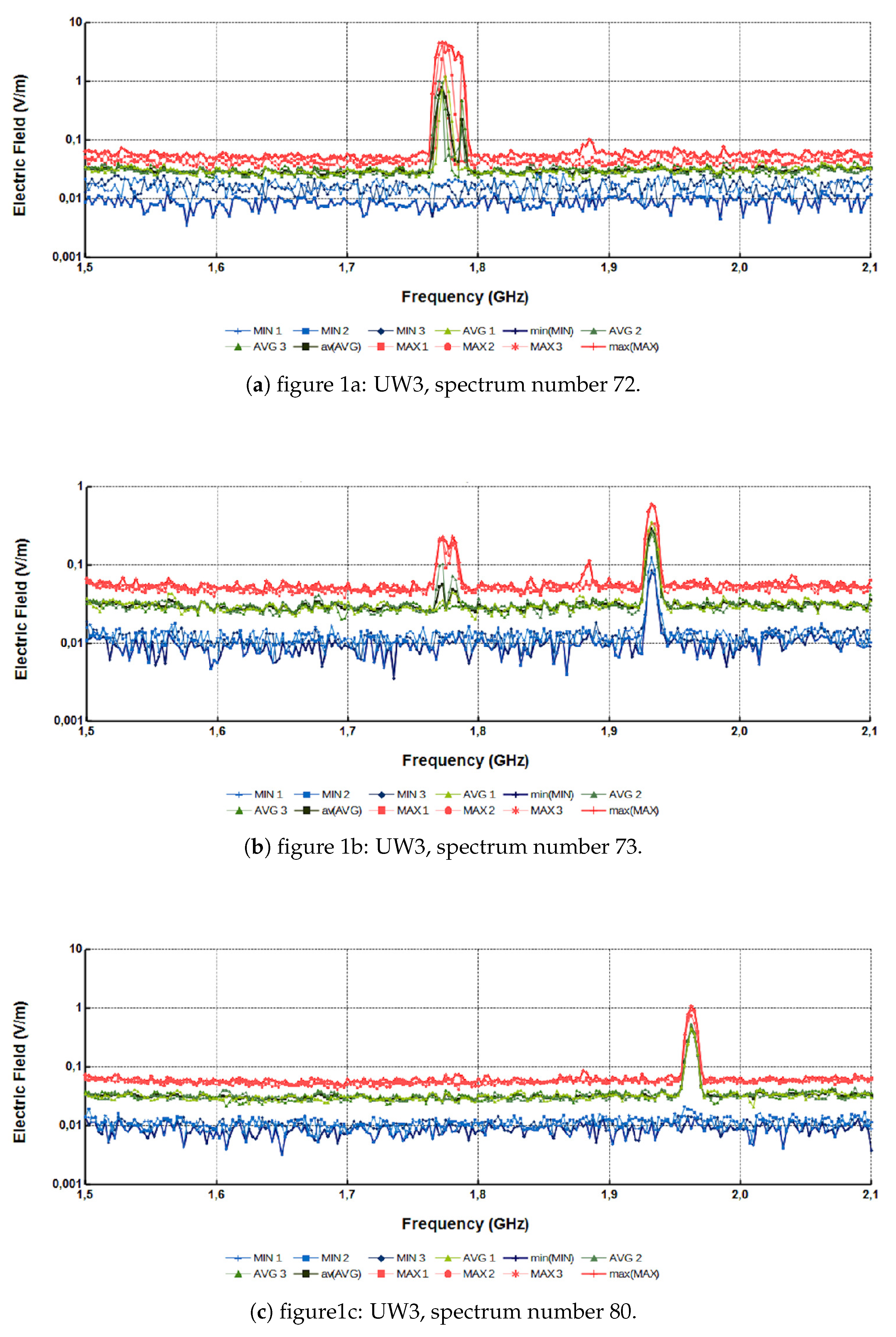
Figure 2.
Characteristic cases with high values at 0 m distance for UW3. The data are the values versus f during the seven minute measurement interval. The legend indicates the number of the spectrum (1-123).
Figure 2.
Characteristic cases with high values at 0 m distance for UW3. The data are the values versus f during the seven minute measurement interval. The legend indicates the number of the spectrum (1-123).
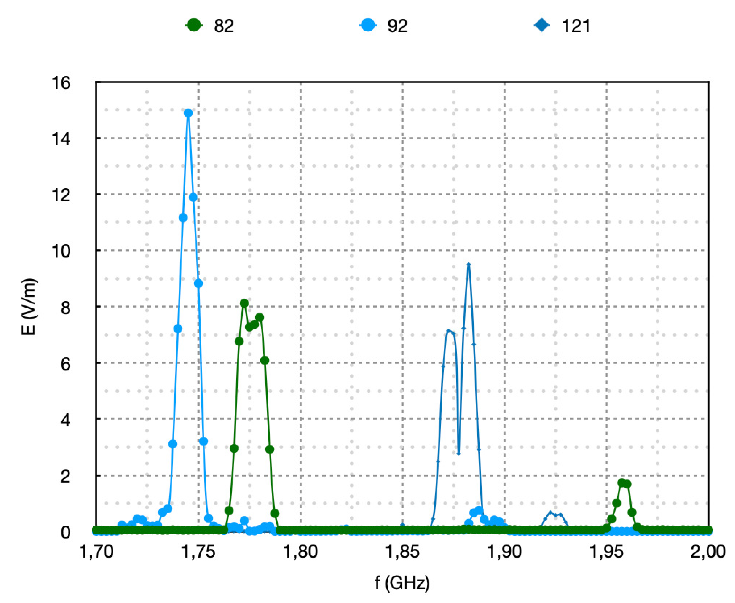
Figure 3.
Characteristic cases with mild values at 0 m distance for UW3. The data are the values versus f during the seven minute measurement interval. The legend indicates the number of the spectrum (1-123).
Figure 3.
Characteristic cases with mild values at 0 m distance for UW3. The data are the values versus f during the seven minute measurement interval. The legend indicates the number of the spectrum (1-123).
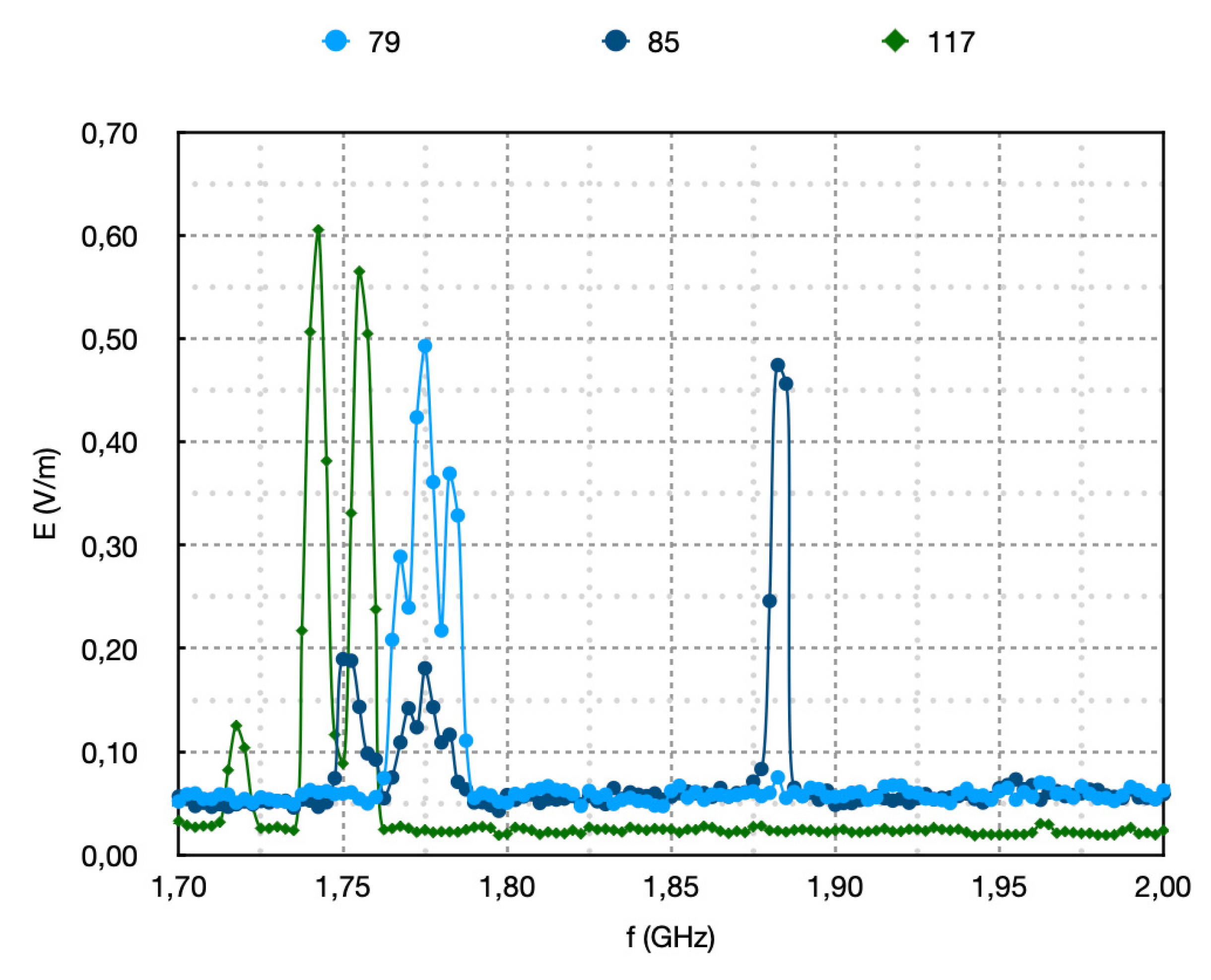
Figure 4.
Characteristic cases with low values at 0 m distance for UW3. The data are the values versus f during the seven minute measurement interval. The legend indicates the number of the spectrum (1-123).
Figure 4.
Characteristic cases with low values at 0 m distance for UW3. The data are the values versus f during the seven minute measurement interval. The legend indicates the number of the spectrum (1-123).
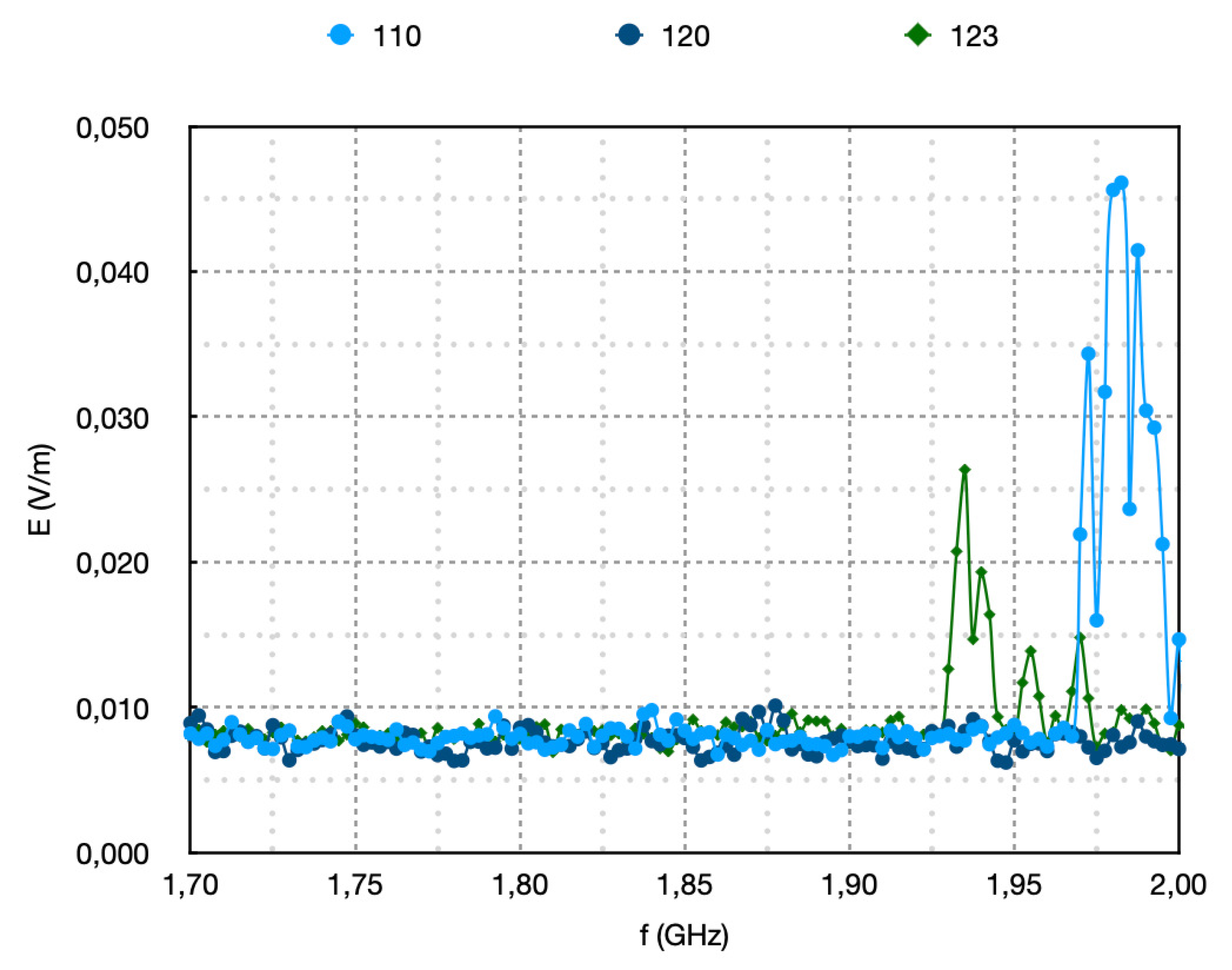
Figure 5.
Box Whiskers plots of measured spectra at distances 0 m and 1 m for the 82 phones from different vendors.The data for all are provided during the seven minute measurement interval.
Figure 5.
Box Whiskers plots of measured spectra at distances 0 m and 1 m for the 82 phones from different vendors.The data for all are provided during the seven minute measurement interval.
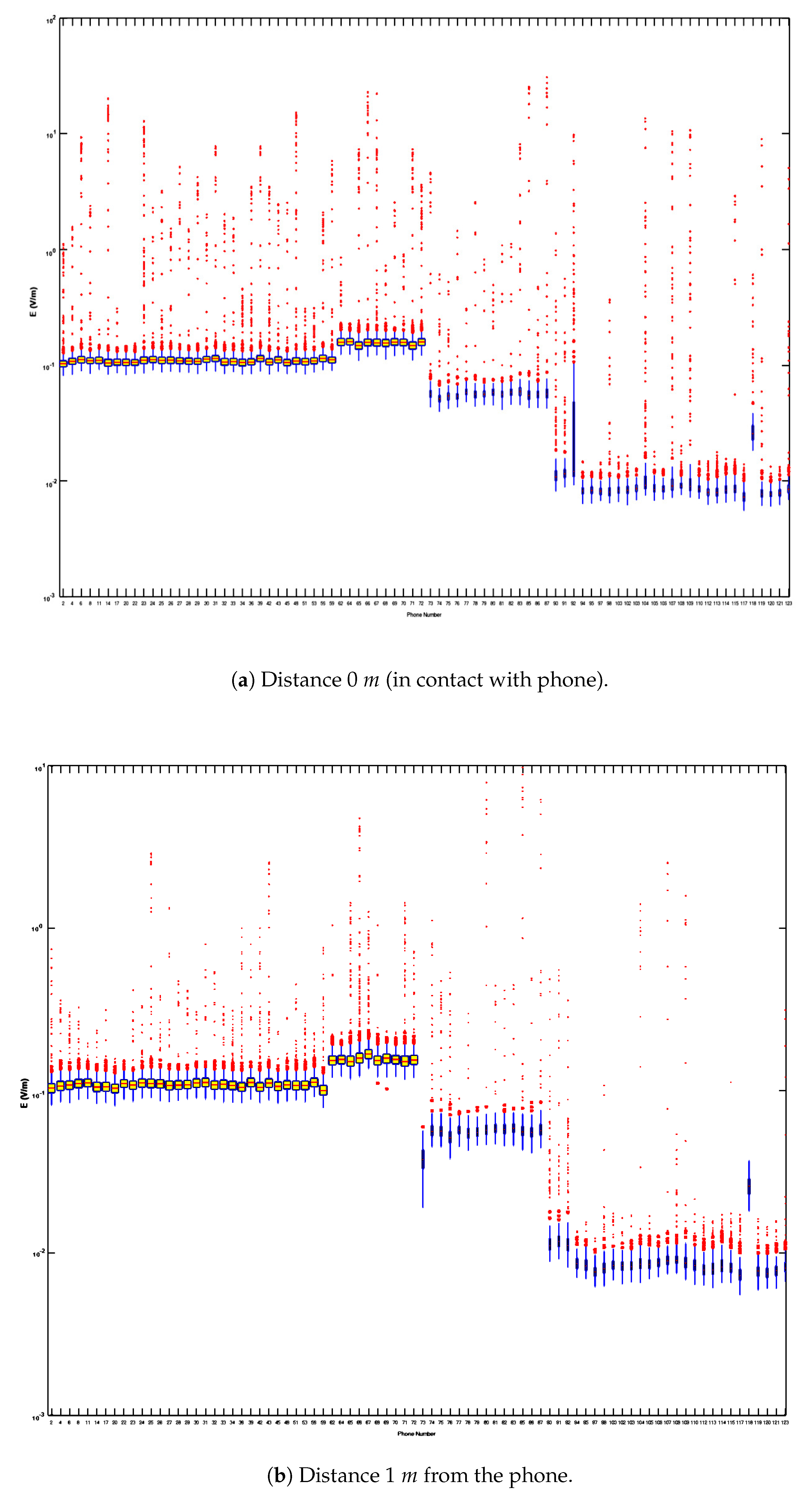
Figure 6.
Box Whiskers plots of measured spectra at distances 0 m and 1 m for the total 123 phones.The data for all are provided during the seven minute measurement interval.
Figure 6.
Box Whiskers plots of measured spectra at distances 0 m and 1 m for the total 123 phones.The data for all are provided during the seven minute measurement interval.
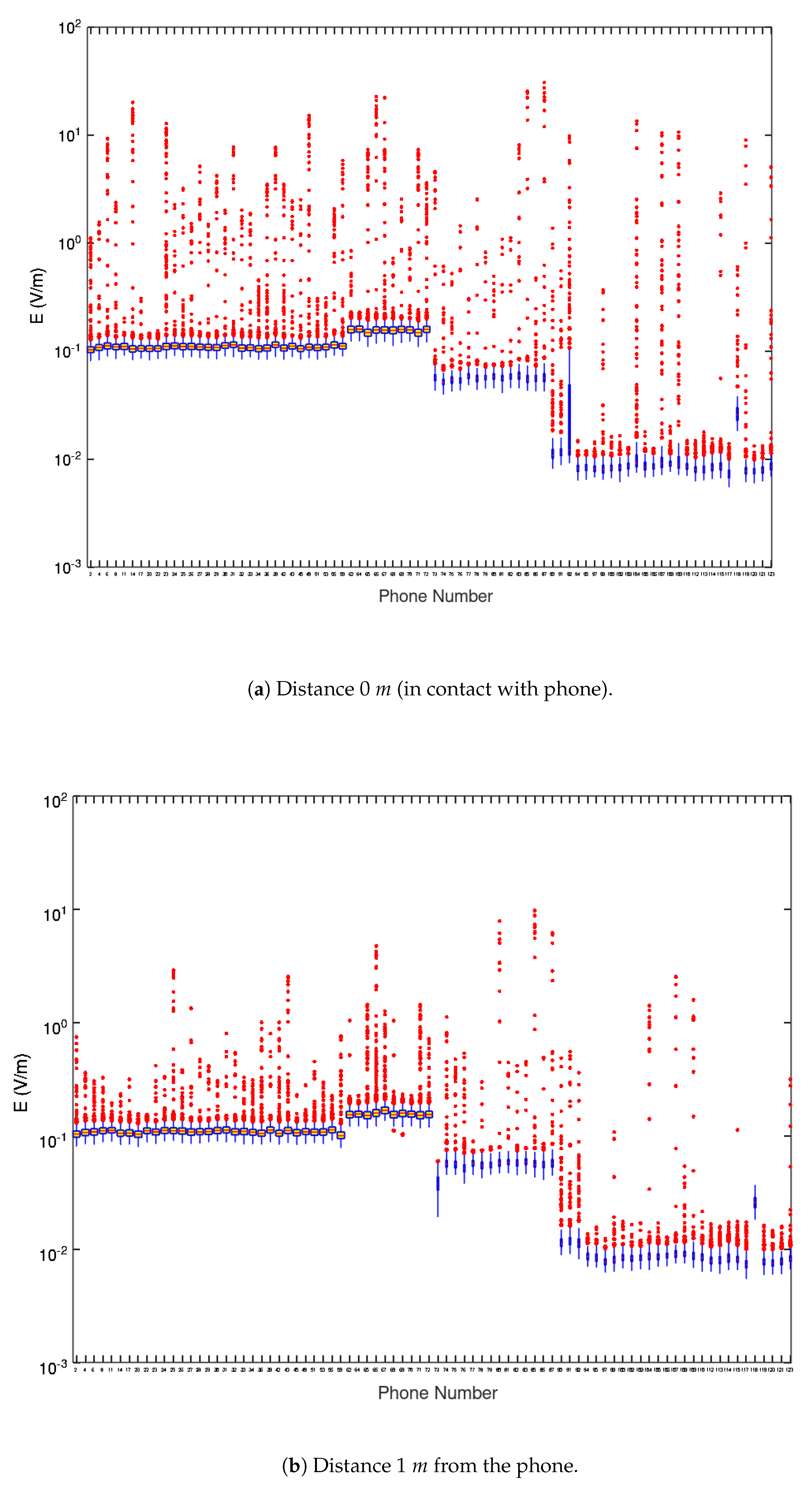
Figure 7.
Box Whiskers plots of measured spectra per Usage Way at distances 0 m and 1 m for the total 123 phones.The data for all are provided during the seven minute measurement interval.
Figure 7.
Box Whiskers plots of measured spectra per Usage Way at distances 0 m and 1 m for the total 123 phones.The data for all are provided during the seven minute measurement interval.
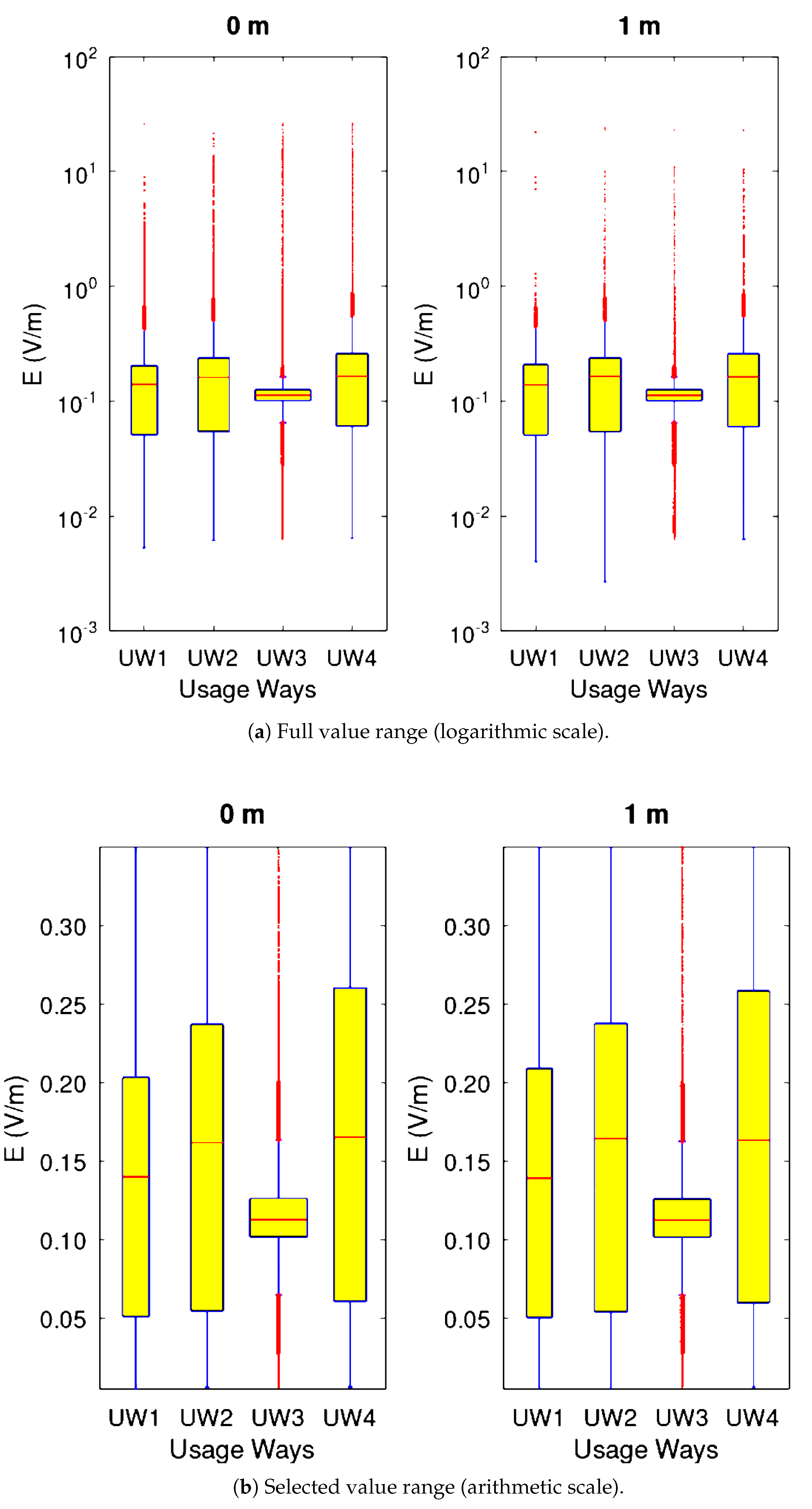

Table 1.
The distinct ways of usage of the investigated mobile phones.
| Code | Way of phone usage |
|---|---|
| UW1 | Standby |
| UW2 | Attempting calling |
| UW3 | Calling |
| UW4 | End of Call |
Table 2.
Descriptive statistics of the UW3 dataset of Figure 7.
Table 2.
Descriptive statistics of the UW3 dataset of Figure 7.
| Distance | Minimum | Q1 | (median value) | Q3 |
|---|---|---|---|---|
| 0 m | 0,0615 | 0,0901 | 0,1186 | 0,1648 |
| 0 m | 0,0552 | 0,0815 | 0,1078 | 0,1551 |
Disclaimer/Publisher’s Note: The statements, opinions and data contained in all publications are solely those of the individual author(s) and contributor(s) and not of MDPI and/or the editor(s). MDPI and/or the editor(s) disclaim responsibility for any injury to people or property resulting from any ideas, methods, instructions or products referred to in the content. |
© 2025 by the authors. Licensee MDPI, Basel, Switzerland. This article is an open access article distributed under the terms and conditions of the Creative Commons Attribution (CC BY) license (http://creativecommons.org/licenses/by/4.0/).
Copyright: This open access article is published under a Creative Commons CC BY 4.0 license, which permit the free download, distribution, and reuse, provided that the author and preprint are cited in any reuse.


