Submitted:
21 March 2025
Posted:
24 March 2025
You are already at the latest version
Abstract
This paper is mainly to do in-depth research on inequalities on symmetric cones. We will conduct further analysis and discussion based on the inequalities we have developed on the second-order cone, and develop more inequalities. According to our past research in dealing with second-order cone inequalities, we derive more inequalities concerning eigenvalue version of Young inequality and trace version of inverse Young inequality. These results coincide with the conclusions on the positive semidefinite cone, which is also a symmetric cone. It is of considerable help to the establishment of inequalities on symmetric cones and the analysis of their derivative algorithms.
Keywords:
symmetric cone
; second-order cone
; positive semidefinite cone
; symmetric cone programming
; Young inequality
; inverse Young inequality
1. Introduction
Optimization theory primarily explores the existence of an optimal solution for an objective function under specific conditions and the methods for finding it. The content includes studying the conditions for the existence of the optimal solution and some related criteria and designing the corresponding algorithm to find the optimal solution. Now, we consider the following nonlinear symmetric cone programming (SCP):
where is a Euclidean Jordan algebra, denotes the associated symmetric cone of invertible squares, is a proper lower semicontinuous convex function. A popular approach to deal with SCP is the proximal point algorithm, which generates a sequence via the following iterative scheme:
Here, is a certain function that satisfies some desirable properties and a positive sequence. The choice of is important, and several well-known examples are the distances induced by the Euclidean norm, the Bregman distance, the proximal distance, the quasi-distance and the -divergence.
We recall that a distance function (or called metric) on a set X is a function satisfying that, for all ,
There are several ways of relaxing the axioms of distance. For example, a semi-distance is defined as a function that satisfies all axioms for a distance with the possible exception of (D4). A quasi-distance is defined as a function that satisfies all axioms for a distance with the exception of (D3).
In the previous research, it can be observed that when an algorithm is designed to solve symmetric cone programming problems and investigate its convergence, it is essential to consider inequalities on symmetric cones. Most of these inequalities differ from those in real numbers. Due to the special algebraic structure, deriving inequalities analogous to fundamental ones in real numbers is not always feasible, such as the most fundamental arithmetic-geometric mean inequality and the Cauchy-Schwarz inequality, among others. Historically, the development of inequalities associated with symmetric cones has been mainly centered on matrix inequalities, as detailed in [1,2].
In fact, there are only a few known inequalities associated with second-order cones. For several years, one of our main research focuses on deriving inequalities associated with second-order cones, including defining the mean and weighted mean, and establishing trace inequalities associated with second-order cones. The main goal of this paper is to establish a series of results analogous to well-known inequalities in matrix analysis. So far, we have accumulated numerous studies on this topic; see [3,4,5,6,7,8].
In this paper, we derive various trace and norm inequalities related to second-order cones. Section 2 provides a review of fundamental concepts concerning symmetric cones, with a particular focus on second-order cones. In Section 3, we explore the Young and inverse Young inequalities associated with second-order cones. Finally, Section 4 discusses potential directions for future research.
Throughout this paper, we denote the n-dimensional Euclidean space endowed with the canonical inner product by , and the norm of x given by is the Euclidean norm. In addition, for any nonempty subset K of , the interior of K is denoted by , and the boundary of K is denoted by .
2. Preliminaries
In this section, we review some fundamental concepts and properties of Jordan algebras, as presented in [9] on symmetric cones and in [10,11,12] on second-order cones (Lorentz cones), which are essential for the subsequent analysis.
A Euclidean Jordan algebra is a finite-dimensional inner product space ( for short) over the field of real numbers equipped with a bilinear map , which satisfies the following conditions:
- (i)
- for all ;
- (ii)
- for all ;
- (iii)
- for all ,
where , and is called the Jordan product of x and y. If a Jordan product only satisfies conditions (i) and (ii) in the above definition, the algebra is said to be a Jordan algebra. If there is a (unique) element such that for all , the element e is called the identity element in . Note that a Jordan algebra does not necessarily have an identity element. Throughout this paper, we assume that is a Euclidean Jordan algebra with an identity element e.
In a given Euclidean Jordan algebra , the set of squares is a symmetric cone[9], TheoremIII.2.1. That is, is a self-dual, closed convex cone, and homogeneous, which means that for any two elements , there exists an invertible linear transformation such that and .
- An element is an idempotent if ,
- An element is called a primitive idempotent if it is nonzero and cannot be written as a sum of two nonzero idempotents.
- The idempotents and are said to be orthogonal if .
In addition, we say that a finite set of primitive idempotents in is a Jordan frame if
Note that whenever . With the above definitions, there is the spectral decomposition of an element x in .
Theorem 1.
[9], heoremIII.1.2 (The Spectral Decomposition Theorem) Let be a Euclidean Jordan algebra. Then there is a number r such that, for every , there exists a Jordan frame and real numbers with
Here, the numbers are called the eigenvalues of x, the expression is called the spectral decomposition of x. Moreover, is called the trace of x, and is called the determinant of x.
The second-order cone (in short SOC), in is an important example of symmetric cones, which is defined as follows:
For , denotes the set of nonnegative real number . Since is a pointed closed convex cone, for any in , we define a partial order on it:
Note that the relation (or ) is only a partial ordering, not a linear ordering in . To see this, a counterexample occurs by taking and in . It is clear to see that , . For any and , we define the Jordan product as
We note that acts as the Jordan identity. Besides, the Jordan product is not associative in general. However, it is power associative, i.e., for all . Without loss of ambiguity, we may denote for the product of m copies of x and for any positive integers m and n. Here, we set . In addition, is not closed under Jordan product.
Given any , it is known that there exists a unique vector in denoted by such that . Indeed,
In the above formula, the term is defined to be the zero vector if , i.e., . For any , we always have , i.e., . Hence, there exists a unique vector denoted by . It is easy to verify that and for any . It is also known that . For more details, please refer to [9,13].
In the setting of second-order cone in , the vector can be decomposed as
where and are the eigenvalues (or spectral values) and the associated eigenvectors (or spectral vectors) of x, respectively, given by
for with being any vector in satisfying . The decomposition is unique if . Accordingly, the determinant, the trace, and the Euclidean norm of x can all be represented in terms of and :
For any function , the following vector-valued function associated with () was considered in [10,11]:
If f is defined only on a subset of , then is defined on the corresponding subset of . The definition (4) is unambiguous whether or . The cases of , , are discussed in [9]. Let m be any real number and , we could define the power of x as
With this definition, we can explore the properties of the Young inequality associated with second-order cones.
In a Euclidean Jordan algebra , for any , the linear transformation is called Lyapunov transformation, which is defined as for all . The so-called quadratic representation is defined by
For any , the endomorphisms and are self-adjoint. We say that two elements x and y of a Euclidean Jordan algebra operator commute if for all , which is equivalent to stating that . For the quadratic representation , if x is invertible, then is invertible with and
To close this section, we summarize some fundamental properties as follows. The proofs are omitted because they can be found in [9,10,13].
Lemma 1.
- (a)
- ;
- (b)
- If , then for all .
- (c)
- .
- (d)
- .
3. Young Inequality and Inverse Young Inequality
Suppose that and with , the Young inequality states that
In 1995, Ando [14] showed the singular value version of Young inequality that
where A and B are positive definite matrices. Huang, Chen, and Hu[7] propose some trace version of Young inequality associated with second-order cones. The authors conjectured the existence of an eigenvalue version of the Young inequality.
Conjecture 1.
For any , there holds
Recently, Huang et al. [8] establish that the Young inequality under the partial order
holds if x and y share the same Jordan frame. Furthermore, it deduces the trace, determinant, and norm version of Young inequalities.
In the following, for any and , we may assume that , . In fact, x and y will share the same Jordan frame if or . We first illustrate some inequalities of eigenvalue associated with second-order cones, and establish the condition that the equality holds.
Lemma 3.
For any , the followings hold
- (a)
- .
- (b)
- .
Proof.
For any and , we note
(a) It is known that by triangle inequality of norm, we have
Hence, we obtain
(b) Similarly, the desired inequality follows by
We complete the proof. □
Proposition 1.
For any , with , the followings hold
- (a)
- (b)
Proof.
According to the decomposition of , it is clear that
since p, q are positive and for .
(a) It follows by Lemma 3 that
(b) Similarly, the desired inequality follows by
The proof is complete. □
Proposition 2.
For any , there holds
Proof.
We note that
Then, the result follows by
where the inequalities hold by triangle inequality and Schwarz inequality. □
Remark 1.
Based on Proposition 1-2, for with , we can establish a picture of the ordered relationship between the eigenvalues of x, y, , as depicted in Figure 1. However, we have no results regarding the relationship between and . In fact, does not always belong to even if . That is, it is possible that .
Proposition 3.
For any , with , there holds
Proof.
First, we write , where
By triangle inequality of norm, it implies that
Then, the first inequality follows by
Similarly, the second inequality holds since
Therefore, we conclude the desired inequalities. □
Remark 2.
According to Lemma 2(b) and the classical Young inequality for real numbers, we can obtain the determinant version of Young inequality in the setting of second-order cone, that is, for with ,
In fact, Huanget al.[4] establish the determinant version of Young inequality based on the SOC weighted mean inequality. However, we obtain a refined inequality by direct computation.
Proposition 4.
For any , with , the following holds
Proof.
Let be expressed as in (5). Thus, we have
Similarly, the other inequality follows by
We conclude the desired result. □
Proposition 5.
For any , the following holds
Proof.
Suppose that and . It is evident that the inequalities hold if or . In fact, the equality will hold if or . We assume that , , which imply and . Then,
where is the angle between and in . We notice that the value of is determined by if , , , are fixed. Let be defined by
The derivative of f is
Then, it is clear that 0, are the only two critical points of f since
Therefore, the extreme values of occur at . For , we have
On the other hand, for , we obtain
Thus, the norm attains the maximum and minimum at and , respectively. The proof is complete. □
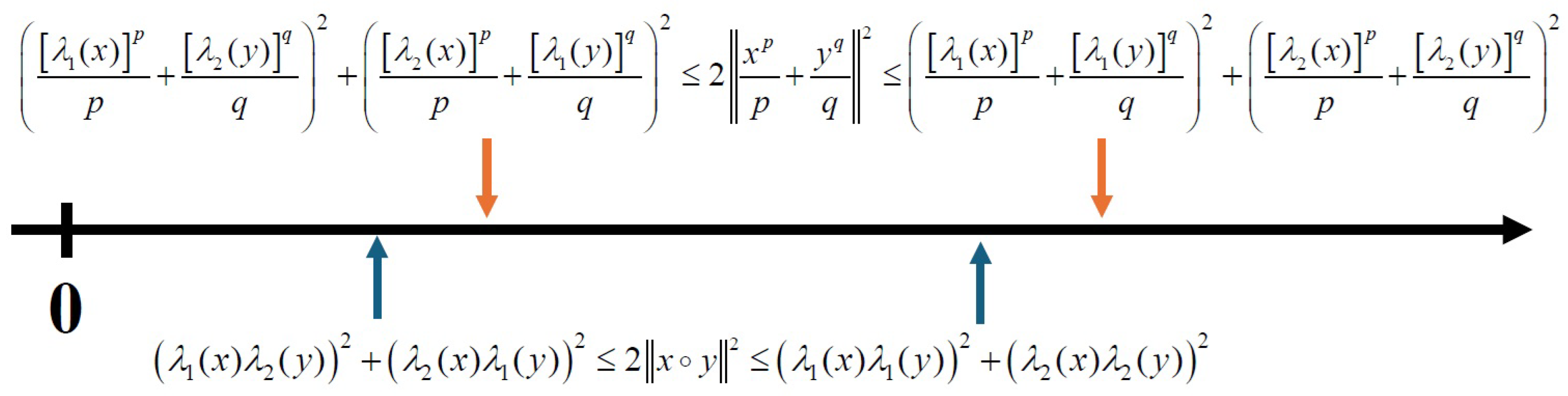
Remark 3.
According to the proof of Proposition 4, we remark that the maximum and minimum of the norm also occur at and , respectively. In addition, for with , we could obtain the relationship between these two maxima and minima by applying the classical Young inequality, see Figure 2. However, we have not reached a conclusion whether the inequality is true or not.
Next, we consider the inverse Young inequality, namely
for and . Manjegani and Norouzi [15] prove an inverse Young inequality for eigenvalues of positive definite matrices, that is,
where A and B are positive definite matrices, and . However, Drury[16] provides counterexamples to (6) for , and slightly modifies inequality (6). He proves that the results hold only for . In the following, we discuss the trace version of inverse Young inequality in the setting of second-order cone.
Theorem 2.
(Inverse Young inequality-Type I) For any , there holds
where .
Proof.
According to Lemma 1(c)(d), the desired result follows by
where the last inequality is due to the inverse Young inequality for positive numbers. □
Corollary 1.
(Inverse Young inequality-Type II) For any , there holds
where .
Proof.
The results follow immediately from the fact that and Lemma 1(b). □
Theorem 3.
(Inverse Young inequality-Type II) For any , if are not in , there holds
where .
Proof.
We note that both and are in . The desired inequality follows by applying Theorem 2 to and . □
Now, we construct a counterexample to elaborate that for any , the eigenvalue version of inverse Young inequality in the SOC setting , that is,
is false if .
Example 1.
Let , . Then we have
and hence, . Therefore,
Example 2.
Let , . Then we have
which says that . Hence,
Which implies
In Example2, we note that it is also a counterexample to the determinant version of inverse Young inequality, that is,
is false for . However, for the other type of determinant version of inverse Young inequality, namely,
we have no conclusion yet.
4. Conclusion
In this paper, we establish several inequalities associated with second-order cones. We discuss the relationship between the eigenvalue and norm of x, y, , in Proposition 1-2 and Proposition 4, respectively. we derive a refined inequality for the determinant version of Young inequality through direct computation. Moreover, we explore the inverse Young inequality in the setting of second-order cones. Our conclusions align with the results established for the positive semidefinite cone, which is also a symmetric cone. We believe that Conjecture1 holds, as computational verification has found no counterexample in . However, directly proving the inequality is challenging due to the algebraic complexity of the expression . There are several directions that are worth further exploration. We outline them as follows.
- (Q1)
- Does the inequality hold or not?
- (Q2)
- Does the inequality hold or not?
We note that Conjecture1 would be wrong if we could show that Q1 is false.
Funding
This work is supported by National Science and Technology Council of Republic of China.
Conflicts of Interest
The authors declare no conflicts of interest.
References
- Bhatia, R. Positive Definite Matrices; Princeton university press, 2005.
- Zhan, X. Matrix Inequalities; Lecture Notes in Mathematics, 1790), Springer-Verlag, Berlin, 2002.
- Chang, Y.-L.; Huang, C.-H.; Chen, J.-S.; Hu C.-C. Some inequalities for means defined on Lorentz cone, Math. Inequal. Appl. 2018, 21(4), 1015–1028.
- Huang, C.-H.; Chang, Y.-L.; Chen, J.-S. Some inequalities on weighted means and traces defined on second-order cone, Linear and Nonlinear Anal. 2019, 5(2), 221–236.
- Huang, C.-H.; Chang, Y.-L.; Chen, J.-S. The P-class and Q-class functions on symmetric cones, J Nonlinear Var. Anal. 2020, 4(2), 273–284.
- Huang, C.-H.; Chen, J.-S. On unitary elements defined on Lorentz cone and their applications, Linear Algebra Appl. 2019, 565, 1–24. [CrossRef]
- Huang, C.-H.; Chen, J.-S.; Hu C.-C. Trace versions of Young inequality and its applications, J Nonlinear Convex Anal. 2019, 20(2), 215–228.
- Huang, C.-H.; Hsiao, Y.-H.; Chang, Y.-L.; Chen, J.-S. On Young Inequality under Euclidean Jordan Algebra, Linear and Nonlinear Anal. 2019, 5(1), 13–31.
- Faraut, J.; Korányi, A. Analysis on Symmetric Cones; Oxford Mathematical Monographs (New York: Oxford University Press), 1994.
- Chen, J.-S. The convex and monotone functions associated with second-order cone, Optimization 2006, 55, 363–385. [CrossRef]
- Chen, J.-S.; Chen, X.; Pan, S.-H.; Zhang, J. Some characterizations for SOC-monotone and SOC-convex functions, J Glob. Optim. 2009, 45, 259–279. [CrossRef]
- Chen, J.-S.; Chen, X.; Tseng, P. Analysis of nonsmooth vector-valued functions associated with second-order cones, Math. Program. 2004, 101, 95–117. [CrossRef]
- Fukushima, M.; Luo, Z.-Q.; Tseng, P. Smoothing functions for second-order-cone complementarity problems, SIAM J Optim. 2002, 12, 436–460. [CrossRef]
- Ando, T. Matrix Young inequalities, Oper. Theory Adv. Appl. 1995, 75, 33–38. [CrossRef]
- Manjegani, S.M.; Norouzi, A. Matrix form of inverse Young inequalities, Linear Algebra Appl. 2015, 486, 484–-493.
- Drury, S. The matrix inverse Young inequality, Electron. J Linear Al. 2023, 39, 151–153.
Figure 1.
Relationship between eigenvalues of x, y, , .
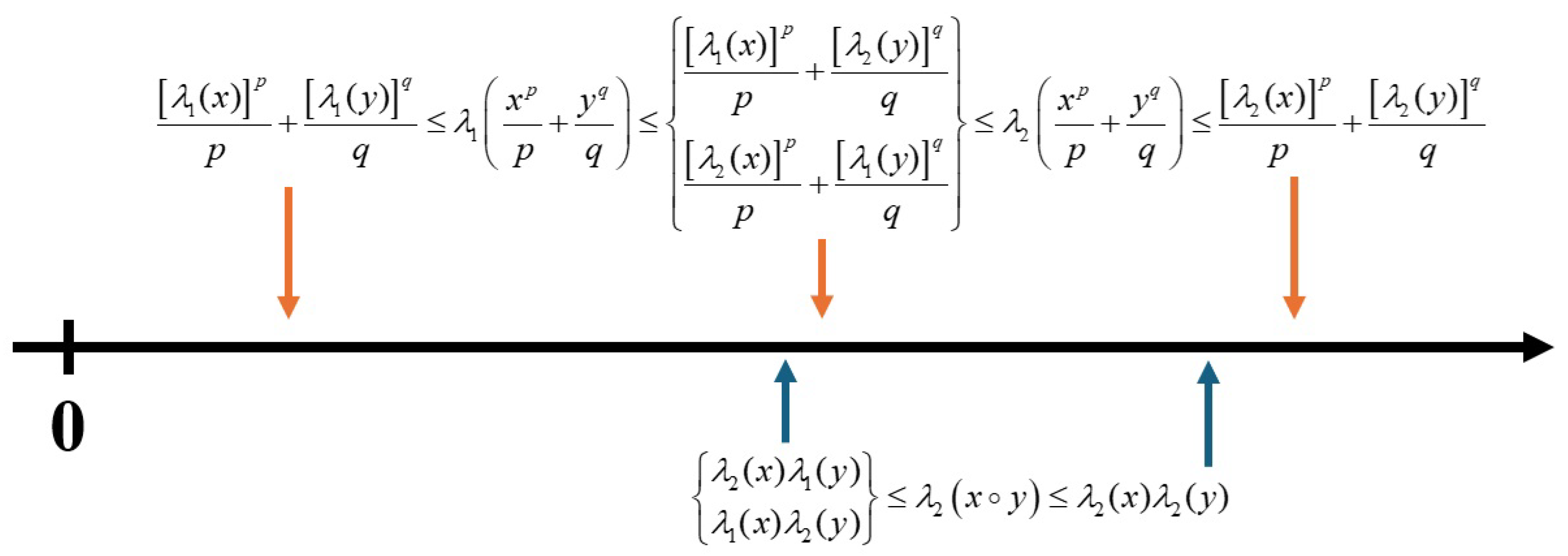
Figure 2.
Relationship between norm of x, y, , .
Disclaimer/Publisher’s Note: The statements, opinions and data contained in all publications are solely those of the individual author(s) and contributor(s) and not of MDPI and/or the editor(s). MDPI and/or the editor(s) disclaim responsibility for any injury to people or property resulting from any ideas, methods, instructions or products referred to in the content. |
© 2025 by the authors. Licensee MDPI, Basel, Switzerland. This article is an open access article distributed under the terms and conditions of the Creative Commons Attribution (CC BY) license (http://creativecommons.org/licenses/by/4.0/).
Copyright: This open access article is published under a Creative Commons CC BY 4.0 license, which permit the free download, distribution, and reuse, provided that the author and preprint are cited in any reuse.


