Submitted:
20 March 2025
Posted:
20 March 2025
You are already at the latest version
Abstract
Plant functional traits are critical indicators of ecosystem health, yet predicting aquatic leaf traits via spectral reflectance remains challenging due to limited sample sizes and the underrepresentation of rare species. We hypothesized that dominant species’ spectral models could infer rare species’ traits even with constrained data. To test this, we measured leaf reflectance spectra and eleven functional traits across diverse freshwater macrophyte species, developing Partial Least Squares Regression (PLSR) models under varying species combinations (All-families, Dominant-families, Non-Cyperaceae, etc.) and sample sizes (40–240). Results demonstrated that species composition exerted greater influence than sample size on validation accuracy for most traits when samples ranged from 120 to 240. A minimum threshold of 160 samples was identified for robust trait prediction, though model performance diverged significantly between All-families and dominant-family combinations, suggesting dominant taxa alone inadequately represent quadrat-level trait diversity. These findings challenge assumptions that dominant species compensate for rare species’ scarcity in spectral modeling. We advocate prioritizing rare species sampling to enhance model generalizability in wetland ecosystems. This work establishes actionable guidelines for scaling spectral trait prediction in marshes, advancing ecological monitoring and restoration efforts.
Keywords:
leaf traits
; spectroscopy
; species combination
; aquatic plan
; Partial least squares regression
1. Introduction
Leaf traits encompass the physiological, morphological, and biochemical characteristics of plant leaves, influencing crucial biological processes such as photosynthesis, primary productivity, and nutrient cycling [1,2,3]. They serve as pivotal factors in plant resource acquisition and allocation, embodying the outcomes of evolutionary and community compositional dynamics shaped by biotic and abiotic environmental constraints that drive multiple ecosystem processes [4,5,6,7]. Chemical traits like Leaf Water Content (LWC), leaf nitrogen, phosphorus, sugars, and starch impact nutrient absorption, growth, and biogeochemical cycling [8,9,10]. Morphological traits such as Leaf Area (LA), Specific Leaf Area (SLA), Equivalent Water Thickness (EWT), and plant height influence biomass, plant drought resistance, and combustibility [11,12]. The different and coordinated expression of these traits determines plant growth and responses to environmental factors, reflecting inherent trade-offs in plant growth strategies [9]. Therefore, a comprehensive understanding of leaf functional traits is imperative for elucidating the consequences of global change on ecological processes [13,14].
Leaf traits influence the optical properties of plants, with varying importance across species and growth forms [15,16]. The spectral bands from Visible light (VIS) to Short-Wave Infrared Radiation (SWIR) reflect the relationships between leaf functional traits and reflectance characteristics [17]. For example, leaf pigments (e.g., chlorophyll) have obvious absorption characteristics in the VIS (400-700nm), leaf structure (e.g., leaf thickness) shows prominent reflection characteristics in the Near Infrared Radiation (NIR, 700-1100nm), and the features of leaf chemical traits (e.g., proteins, lignin, and cellulose) are reflected to varying degrees in the SWIR (1100-2500nm) [18,19]. Studies have found that for wetland aquatic plants, chlorophyll and SLA explain 60% of the variation in the spectrum, and nutrients in leaf tissues also influence spectral reflectance [20,21,22]. Researchers have leveraged plant spectra reflectance data collected by diverse sensors to predict traits using statistical or physical methods [23].
Numerous studies have compared these methods, for instance, Liu et al. (2023) assessed the predictive capabilities of PLSR, Support Vector Regression (SVR), Gaussian Process Regression (GPR), and Random Forest Regression (RFR) for estimating leaf nutrients at the leaf scale. They demonstrated that PLSR and SVR yielded the most accurate predictions for nine nutrients [24]. Feilhauer et al. examined the efficacy of PLSR, SVM, and RFR in predicting chlorophyll, dry matter content, and water content using leaf reflectance, concluding that PLSR outperformed the other methods [25]. Further research has corroborated the effectiveness of the PLSR, which involves transforming spectral reflectance into a concise set of orthogonal features (referred to as "latent factors") and then linearly regressing these features against leaf biochemicals or morphological traits. This approach has proven effective in elucidating the relationship between spectral reflectance and leaf traits [22,26,27,28].
Generally, Leaf Mass per Area (LMA), Leaf Dry Matter Content (LDMC), N, and EWT are accurately predicted using PLSR, yet some traits exhibit lower accuracy. For instance, Kothari et al. found that spectral predictions for certain trace nutrients like P and Mg exhibited lower accuracies (with R2 of 0.3) in their investigation of seven plant types [29]. In Rebelo et al. prediction of morphological traits such as SLA and leaf length-width ratio, the model accuracy ranged from 0.19 to 0.39, while for chemical traits like silicon and cellulose content, R2 were 0.37 and 0.57, respectively [15]. Several studies have shown that the correlation between leaf spectral and leaf traits is influenced by phenological changes [30,31]. In addition, other research has shown that spectral mixing played a critical role in the accuracy of leaf trait estimates [32]. However, other influencing factors of trait prediction accuracy are still underexplored.
The quantity of samples is a critical factor in constructing models for the spectral prediction of leaf traits [33]. While leaf samples are relatively easy to obtain in forest or grassland ecosystems, the growth environments of wetland aquatic plants are frequently waterlogged and featuring complex microtopography [34], which complicates the sampling process. Additionally, herbaceous plants particularly those from families such as Cyperaceae and Gramineae typically have slender leaves, which further making it even more difficult to measure leaf spectral and traits for developing reliable spectral models. Therefore, identifying the minimum sample size necessary for accurately predicting leaf traits in marshes aquatic plants is crucial to improving sampling efficiency. Meanwhile, Cyperaceae and Gramineae are the dominant plant families in most marshes, it can be challenging to obtain enough quantity of sample for rare species. Therefore, there is a need to explore an alternative predictive method for estimating the leaf traits for rare species.
In this paper, we aim to predict leaf traits with leaf spectra in typical marsh in Northeast China. Our objective is to explore two hypotheses regarding the spectral inversion of leaf functional traits. Hypothesis 1 (H1): we hypothesize that the sample size affects the accuracy of prediction models. Hypothesis 2 (H2): we posit that the leaf traits of rare species can be inferred from the modeling results of the dominant species.
2. Materials and Methods
2.1. Study Area
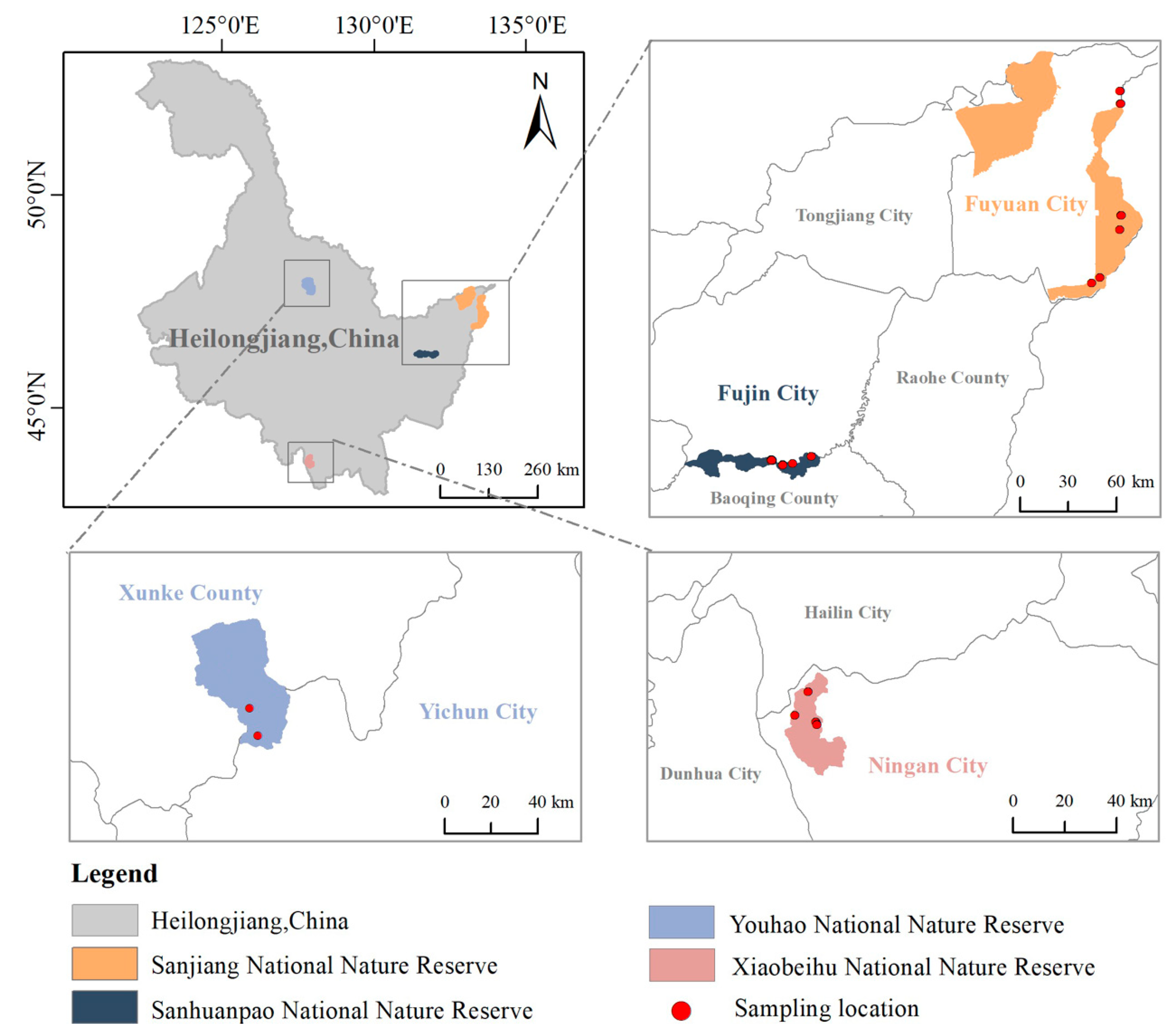
We conducted sampling across various regions of Heilongjiang Province, covering the representative distribution areas of typical marshes. From June to September during 2021-2023, leaf and spectral samples were collected from four national nature reserves in Heilongjiang Province, namely Xiaobeihu National Nature Reserve (XBHNNR), Sanhuanpao National Nature Reserve (SHPNNR), and Sanjiang National Nature Reserve (SJNNR), Youhao National Nature Reserve (YHNNR). A total of 16 plots (30 m × 30 m) were established across these reserves.
Xiaobeihu National Nature Reserve (128°33´07"-128°45´48" E, 44°03´16"-44°18´59" N) experiences a temperate continental climate, characterized by a mean annual temperature of approximately 2.5°C and an average annual precipitation of around 650 mm. The reserve features a diverse range of habitat types, with the dominant community being the Carex community. Key dominant species include Carex appendiculata, Carex schmidtii, Deyeuxia purpurea, and Sanguisorba tenuifolia. Additionally, Saussurea amara, Carex meyeriana, and Filipendula palmata are among the accompanying dominant species found in the area.
Sanhuanpao National Nature Reserve (132°12′18″-132°57′25″ E, 46°45′08″-46°51′41″ N) showcases a characteristic swampy low-river floodplain landscape, characterized by low-lying terrain and an average elevation of 60 m. It experiences an average annual temperature of approximately 2.7°C, accompanied by a mean annual precipitation of around 550 mm. There are diverse community types, including Glyceria acutiflora-Deyeuxia purpurea communities, Carex appendiculata-Deyeuxia purpurea communities, Bidens pilosa-Valeriana officinalis communities, Deyeuxia purpurea communities, and Glyceria acutiflora communities. However, the species composition within these communities tends to be relatively homogeneous, with some communities characterized by the presence of only one species. The dominant species in this area include Glyceria acutiflora, Deyeuxia purpurea, and Carex appendiculata.
Sanjiang National Nature Reserve (134°36′12″-134°4′38″ E, 47°44′40″-48°8′20″ N) encompasses a low-impact plain marsh wetland characterized by low-lying terrain, with elevations ranging from 34 m to 80 m. The soil in this region is characterized by high humidity and abundant organic matter content. It experiences an average annual temperature of approximately 2.2°C, accompanied by a mean annual precipitation of about 600 mm. The area predominantly features the Deyeuxia purpurea-Carex appendiculata community and the Deyeuxia purpurea-Carex miyabei community. The dominant species include Carex appendiculata and Deyeuxia purpurea, alongside coexisting species such as Lythrum salicaria, Hypericum japonicum, and Sanguisorba tenuifolia.
Youhao National Nature Reserve (128°10′15″-128°33′25″ E,48°13′07″-48°33′15″ N) is characterized by a temperate continental climate, with an average annual temperature of approximately 0.4°C. The area has a diverse of marsh types, comprising forested swamps, shrub swamps, herbaceous marshes, and sphagnum bogs. The dominant species in this area include Carex schmidtii, Carex miyabei, Sphagnum palustre, and Filipendula palmata.
Figure 1.
Distribution of the study site and sampling plots.
2.2. Data and Methods
2.2.1. Plant Sample Collection and Species Combinations
Within each of the plots, 11 smaller quadrats (1 m × 1 m) were randomly established (except YHNNR). From these, we randomly selected 5 quadrats for the collection healthy and undamaged whole plant, 420 samples from 40 species were utilized for trait measurements and data analysis. Among these, the dominant families were Cyperaceae, Gramineae, Rosaceae, Compositae, and Geraniaceae. We created several subsets based on different species combinations to test whether models built with dominant species could predict rare species. Specifically, the species combinations inclusion of the following families: All-families (control group, nT = 420), Dominant-families (Cyperaceae (n = 137), Gramineae (n = 142), Rosaceae (n = 65), Compositae (n = 18), and Geraniaceae (n = 7), nT = 369), and Non-Cyperaceae families(Gramineae, Rosaceae, Compositae, Geraniaceae, and Others (n = 51), nT = 283), Gramineae-Cyperaceae families (nT = 279), and Cyperaceae family (Table 1).
2.2.2. Leaf Spectra Measurement
Plant leaves were promptly stored in a portable refrigerator with ice bag upon collection, and spectral measurements were conducted within 6 hours of collection. From 2021to 2022, for each sample, three leaves were selected, arranged in parallel, and the spectral reflectance of fresh plant smooth leaves was measured using the ASD LabSpec 2500 spectrometer, which covers a spectral range of 350-2500 nm (with a spectral resolution of 3 nm @ 350-1050 nm and 10 nm @ 1000-2500nm). For 2023, using RS-5400 high resolution spectrometer measured the fresh plant spectral reflectance, which covers a spectral range of 350-2500 nm (with a spectral resolution of 2.5nm @ 700nm, 5.5nm @ 1500nm, and 5.8nm @ 2100nm). Five measurements were taken per leaf to ensure accuracy. The spectral data were processed using the Savitzky–Golay (S-G) filtering method in the hsdar package [35] in R software (version 4.1.1), and all spectral data were resampled to 1nm. Finally, trimmed to the 400-2400 nm to obtain spectra with high signal-to-noise ratio. Notably, outliers were observed within the 1830-1884 nm range, and removed, along with any erroneous or outlier spectra data.
2.2.3. Spectral Difference Analysis
To analyze spectral differences among plant families, we employed the Bhattacharyya distance [36,37] (Eq. 1) to quantify the disparities between individuals of two distinct growth forms across the 400-1829nm, 1885-2400nm spectral range (Figure S1). This approach facilitated the identification of wavelengths exhibiting maximum distinction between the groups. The Bhattacharyya distance (B) has proven effective in delineating differences between species and plants with varying growth habits [38,39].
where and represent the mean values across all spectral bands for species i and j, respectively. and denote the covariance matrices for each species, and represents the pooled covariance matrix.
2.2.4. Measurement and Analysis of Chemical and Morphological Traits
Morphological traits were measured immediately after the leaf spectral measurements. Three leaves were scanned and weighed with an accuracy of 0.001 g to obtain LA and leaf fresh weight. A total of eleven leaf traits were measured, encompassing SLA, LMA, EWT, LWC, N, P, N:P, cellulose, lignin, sugar, and starch. LMA was calculated as the ratio of dry leaf mass to LA, while SLA represents the reciprocal of LMA. EWT and LWC were calculated using the formulas (leaf fresh weight - leaf dry weight) / LA and (leaf fresh weight - leaf dry weight) / leaf fresh weight, respectively [40].
The collected leaf biomass samples were dried in an oven at 60°C for 48 hours and then ground through a 100-mesh sieve for the measurement of leaf chemical traits. Nitrogen (N) content was determined using a fully automated Kjeldahl nitrogen analyzer (Model: FOSS 8400, Manufacturer: FOSS, Denmark). Cellulose and lignin were measured using an ANKOM A200i fiber analyzer utilizing an acidic washing method. Sugar and starch contents were assessed following the method outlined by Lindroth et al [41]. Phosphorus (P) content was determined using a CEM microwave digestion system (Model: MARS 6 CLASSIC, Manufacturer: CEM, USA) to disintegrate the sample solution. After the disintegration process, 2 ml of the liquid to be measured was extracted, and then 2 ml of (NH4)2MnO4 solution, 1 ml of Na2SO3 solution, and 1 ml of hydroquinone solution were added. The mixture was then made up to 25ml with distilled water, and the absorbance of phosphorus was measured using a UV spectrophotometer. The phosphorus content in the samples was subsequently calculated based on a standard curve.
To analyze the traits variation across plant families, we conducted comparisons using ANOVA [42]. Given that the data did not exhibit normal distribution or unequal in variance, we employed the Kruskal-Wallis analysis to compare median differences among three or more independent sample groups [43] (Eq. 2). Furthermore, pairwise comparisons between plant families were conducted using Wilcoxon analysis.
where H is the Kruskal-Wallis statistic, k is the number of groups, N is the total number of samples, is the rank sum of the j group, and is the sample size of the j group.
2.2.5. Impacts of Sample Size and Species Combinations Setup
In terms of sample size, we set six levels: 40 samples (S40), 80 samples (S80), 120 samples (S120), 160 samples (S160), 200 samples (S200), and 240 samples (S240). Regarding species combination, we configurated five combinations of the All-families (AF), Dominant-families (DF), Non-Cyperaceae (NC), Cyperaceae-Gramineae (CG), and Cyperaceae (CY). To remove outliers, after generating predicted values for all samples, we recalculated the bias in the data. Subsequently, samples with deviations exceeded 1.5 times the standard deviation were removed twice.
To separate impacts of sample size and species combination on the precision of spectral models predicting leaf traits, we developed a multivariate linear regression model using the lm function. We set different sample size levels of S120, S160, S200, and S240 for each species combination (except for the CY, the total sample size is about 80). The sample size and species combination served as predictors for the model's coefficient of determination (R2). Additionally, we assessed the contribution of each variable to the model's predictive performance using three methods ("First", "Last", and "Lmg") from the calc. relimp function in the Relaimpo package [44].
2.2.6. Prediction of Leaf Traits by Leaf Spectra
This study modeled the relationship between leaf spectra and traits with a commonly used approach, namely Partial Least Squares Regression (PLSR). PLSR can address the multicollinearity in spectra by reducing the number of predictor variables to a smaller set of uncorrelated variables, subsequently performing least squares regression on this subset [45,46,47]. We predicted eleven leaf functional traits using spectral data from different sample sizes and species combinations, and developed the PLSR models using the pls package [48] in R4.1.1.
Each dataset was divided into a calibration set (70%) and a validation set (30%) to ensure that both sets covered the range of each trait. To mitigate overfitting, we optimized the number of PLSR components in the final model by minimizing the Root Mean Square Error (RMSE) of the prediction residuals [49]. We iteratively sampled the calibration set 50 times to generate 50 models, then averaged the model coefficients to derive an average PLSR model, which served as the final model. Model fitting and prediction accuracy were assessed using the coefficient of determination (R2), RMSE, and Relative Root Mean Square Error (RRMSE = RMSE/range). Additionally, differences in model accuracy across species combinations were compared by Wilcoxon analysis.
Finally, the Variable Importance of Projections (VIP) was computed for each species combinations model to identify the spectral regions contributing most to the prediction of each leaf trait. VIP was calculated as the weighted sum of squares of the PLS-weights, with weights derived from the variance of the response variables explained by each PLS component [50].
3. Results
3.1. Traits Variation Among Families
The distribution of leaf functional traits across various plant families is shown in Figure 2. Kruskal-Wallis analysis revealed differences in 10 traits among families (p < 0.05, Table S1), excluding N. Pairwise Wilcoxon comparisons revealed significant differences between Cyperaceae and other plant families in LMA, SLA, P, and N:P. While Cyperaceae and Compositae showed similar values for sugar, starch, lignin, and N content, they differed significantly in all other traits (Figure 2).
3.2. Model Performance of Different Sample Sizes
Model accuracy improved and RRMSE decreased as sample size increased, though this relationship varied among traits. For cellulose and starch, model accuracy declined significantly when sample size below 80, while N, P, and N:P models showed marked accuracy decreases below 40 samples. Models exhibited high variability with sample sizes under 120 but achieved optimal validation accuracy above 160 samples for all traits (Figure 3, Table S2).
3.3. Model Performance for Different Species Combinations
Different species combinations showed distinct effects on trait model accuracy. LMA and sugar had the highest model accuracy in CY ( = 0.73,RRMSELMA = 10.68%, = 0.56, RRMSESugar = 15.75%), while for cellulose, LWC, and EWT, the model accuracy was the highest in NC ( = 0.63, RRMSECellulose = 13.70%, = 0.85, RRMSELWC = 7.34%, = 0.55, RRMSEEWT = 12.53%). N, P, and lignin had the highest model validation accuracy in CG ( = 0.87,RRMSEN = 9.41%, = 0.54,RRMSEP = 12.76%, = 0.36, RRMSELignin = 17.96%, Figure 4). Overall, N (R2=0.87) had the highest model accuracy in all traits, follow by LWC (R2=0.85, Table S3).
Wilcoxon analysis revealed that model validation accuracy was comparable between AF and DF for SLA, P, and N:P. Similarly, no differences in model accuracy were observed for lignin, starch, and sugar between AF and NC, or for LMA across AF, CG, and NC. However, EWT, LWC, and cellulose models showed significant accuracy differences among AF and other species combinations (Figure 5).
3.4. Variable Importance of PLSR Models for Different Species Combinations
Analysis of VIP values revealed key spectral wavelengths for trait prediction across species combinations. While important wavelengths varied among combinations, most traits showed consistent peaks near 700 nm in the red edge region. The ranges of 400-700 nm and 2000-2400 nm were crucial for trait prediction across all species combinations (Figure S2, Table S4). Notably, CY showed distinct VIP patterns, with significantly higher values for N, lignin, and sugar in the 400-700 nm range compared to other combinations.
4. Discussion
4.1. Optimal Sample Size for High Predictive Accuracy of PLSR Model
Previous PLSR models for plant leaf trait prediction typically used hundreds of samples [33,40], yet collecting such large datasets in wetland ecosystems presents unique challenges. The process is time-consuming and particularly difficult for rare species, thus obtaining adequate leaf samples is often impractical. To determine the optimal sample size for wetland aquatic plant trait prediction, we employed random sampling at different levels. Our analysis revealed that validation accuracy plateaus above 160 samples for most leaf traits. Although obtaining complete trait ranges in field measurements remains challenging [33], it is important to note that limited trait distribution in validation datasets can affect model accuracy [51]. This issue is particularly relevant for wetland ecosystems, where environmental conditions can vary significantly. While Helsen et al. reported optimal sample sizes of 100-160 for PLSR spectral prediction models [33], our more comprehensive dataset suggests that 160-240 samples are necessary for reliable model training. This higher recommended range reflects the broader trait variability typically found in aquatic plants.
4.2. Species Combinations Played a More Substantial Role in Predicting Most Traits
Model validation accuracy varied significantly across species combinations, with performance differing by both trait type and species composition (Figure 5). Some traits, particularly starch and lignin, showed consistently low accuracy across combinations, reflecting the complex interactions among multiple traits within each spectral band [16,52]. Spectral importance analysis through VIP values revealed consistent patterns across traits, despite variations among species combinations. Most traits showed characteristic peaks near 700 nm in the red edge spectral region, corroborating the significant bands previously identified by Wang et al. [30,53]. These findings align with Thomson et al. which highlighted the importance of red-edge and NIR regions for trait prediction, particularly when SWIR data is unavailable [11]. Future research should investigate how spectral band selection could improve leaf trait prediction accuracy.
The dominant families (Cyperaceae, Gramineae, and Rosaceae) of our dataset contrasted with rare families represented by few species. Given the challenges in measuring leaf traits of rare species, using dominant species models to predict rare species traits would be advantageous if model performance was consistent across species combinations. However, our analysis revealed that most traits are significantly influenced by species combinations (Figure 5). Multiple linear regression analysis showed that species combinations had a stronger impact on model validation than sample size for most traits, though LMA, N:P, and starch were particularly sensitive to sample size (Figure 6). These findings indicate that models based solely on dominant species cannot adequately capture the full trait spectrum, emphasizing the necessity of including rare species in field sampling protocols.
4.3. N and LWC Can Be More Accurate Predicted by Leaf Spectra of Aquatic Plants
Our PLSR models for eleven leaf functional traits showed calibration R² ranging from 0.22 to 0.89 and validation R² from 0.12 to 0.87. Based on Kothari’s standards [29], most traits showed moderate to low accuracy in All-families combinations, except for N (R² = 0.87) and LWC (R² = 0.85), which achieved high accuracy. These results align with previous prediction accuracies reported in wetland and grassland ecosystems [32,40,54]. For example, PROSPECT and PLSR models achieved average accuracies around 0.4 for LMA and EWT for aquatic plants [55,56], comparable to our findings for LMA (R² = 0.32-0.73) and EWT (R² = 0.19-0.55). However, these accuracies were lower than those reported in forest ecosystems, where Wang et al. achieved R² up to 0.9 for LMA and EWT [53]. N showed consistently high prediction accuracy (R² > 0.8) across all species combinations, exceeding typical accuracies with R² of around 0.7 reported in previous studies [29,32,57]. LWC predictions were improved when modeling with Non-Cyperaceae samples. Given the sensitivity of LWC to SWIR regions [58,59], future research should investigate whether SWIR-specific modeling could enhance the prediction accuracy.
5. Conclusions
This study explored the factors influencing the accuracy of spectral inversion modeling for leaf traits across different species combinations and sample sizes in aquatic plants. The findings revealed that species combinations significantly impacted modeling accuracy. The N model for the Cyperaceae-Gramineae group achieved the highest accuracy (=0.87), followed by the LWC (=0.85) model in the Non-Cyperaceae group. The VIP values varied across species combinations but showed consistent peak patterns. Sample size was another critical factor driving model performance, with a minimum of 160 samples required to accurately predict most leaf traits using PLSR. These results highlight the complex interplay between species combinations, sample size, and model accuracy in the spectral prediction of plant functional traits. However, this study did not address other important factors, such as phenology and spectral combinations. Future research will incorporate these factors to develop more robust models for the spectral inversion of plant functional traits.
Supplementary Materials
The following supporting information can be downloaded at the website of this paper posted on Preprints.org.
Author Contributions
Conceptualization, Y.S., and Y.Y.; methodology, Y.S.; data curation, Y.S., Y.F., H.Y, and Y.L; writing—original draft preparation, Y.S.; writing—review and editing, Y.S., Y.Y., Z.W., Y.F., L.W., W.W., and H.Y; visualization, Y.S., and X.Z; supervision, Y.Y.; funding acquisition, Y.Y. All authors have read and agreed to the published version of the manuscript.
Funding
This research was funded by National Natural Science Foundation of China, grant number No. 42471138” and the National Key R&D Program of China, grant number 2022YFF1300903.
Data Availability Statement
Data and code[60] are provided as private-for-peer review via the following link: [https://figshare.com/s/e3df47ed7b55a57dabb3].
Acknowledgments
We are grateful to the colleagues from the nature reserves for their support in our field sampling.
Conflicts of Interest
The authors declare no conflicts of interest.
Abbreviations
The following abbreviations are used in this manuscript:
| PLSR | Partial Least Squares Regression |
| LWC | Leaf Water Content |
| LA | Leaf Area |
| SLA | Specific Leaf Area |
| EWT | Equivalent Water Thickness |
| LMA | Leaf Mass per Area |
| N | Nitrogen |
| P | Phosphorus |
| LDMC | Leaf Dry Matter Content |
| VIS | Visible light |
| SWIR | Short-Wave Infrared Radiation |
| SVR | Support Vector Regression |
| GPR | Gaussian Process Regression |
| RFR | Random Forest Regression |
| XBHNNR | Xiaobeihu National Nature Reserve |
| SHPNNR | National Nature Reserve |
| SJNNR | Sanjiang National Nature Reserve |
| YHNNR | Youhao National Nature Reserve |
| S40 | 40 samples |
| S80 | 80 samples |
| S120 | 120 samples |
| S160 | 160 samples |
| S200 | 200 samples |
| S240 | 240 samples |
| AF | All-families |
| DF | Dominant-families |
| NC | Non-Cyperaceae |
| CG | Cyperaceae-Gramineae |
| CY | Cyperaceae |
| RMSE | Root Mean Square Error |
| RRMSE | Relative Root Mean Square Error |
| VIP | Variable Importance of Projections |
References
- Violle, C., et al., Let the concept of traits be functional! Oikos, 2007. 116.
- Butler, E.E., et al., Mapping local and global variability in plant trait distributions. Proceedings of the National Academy of Sciences, 2018. 114(51): p. 10937-10946.
- Ferrier, S. and A. Guisan, Spatial modelling of biodiversity at the community level. Journal of Applied Ecology, 2006. 43(3): p. 393-404.
- Clark, C.M., et al., Testing the Link between Functional Diversity and Ecosystem Functioning in a Minnesota Grassland Experiment. Plos One, 2012. 7(12): p. e52821.
- Thomas, H.J.D., et al., Global plant trait relationships extend to the climatic extremes of the tundra biome. Nature Communications, 2020. 11(1): p. 1351.
- Kattge, J., et al., TRY plant trait database – enhanced coverage and open access. Global Change Biology, 2020. 26(1): p. 119-188.
- Michaletz, S.T., et al., The energetic and carbon economic origins of leaf thermoregulation (vol 2, 16129, 2016). Nature Plants, 2016(9): p. 2.
- Poorter, H.N., L.W. U.Poorter, and R. I. J.Villar, Causes and consequences of variation in leaf mass per area (LMA): a meta-analysis. The New Phytologist, 2009. 182(4): p. 565.
- Díaz, S., et al., The global spectrum of plant form and function. Nature, 2015. 529: p. 167-171.
- Smart, S.M., et al., Leaf dry matter content is better at predicting above-ground net primary production than specific leaf area. Functional Ecology, 2017. 31: p. 1336-1344.
- Thomson, E.R., et al., Multiscale mapping of plant functional groups and plant traits in the High Arctic using field spectroscopy, UAV imagery and Sentinel-2A data. Environmental Research Letters, 2021. 16(5): p. 055006.
- Inge, J., et al., Arctic shrub effects on NDVI, summer albedo and soil shading. Remote Sensing of Environment, 2014. 153: p. 79-89.
- Rogers, A., et al., A roadmap for improving the representation of photosynthesis in Earth system models. New Phytologist, 2017. 213: p. 22-42.
- Fatichi, S., et al., Modelling carbon sources and sinks in terrestrial vegetation. New Phytologist, 2018. 221(2): p. 652-668.
- Rebelo, A.J., et al., Can wetland plant functional groups be spectrally discriminated? Remote Sensing of Environment, 2018. 210: p. 25-34.
- Marín, S.d.T., et al., Spectral signatures of conifer needles mainly depend on their physical traits. Polish journal of ecology, 2016. 64: p. 1-13.
- Jacquemoud, S. and S. Ustin, Leaf Optical Properties. 2019: Cambridge University Press.
- Katja, K., D. Gradinjan, and A. Gaberik, Epiphyton alters the quantity and quality of radiation captured by leaves in submerged macrophytes. Aquatic Botany, 2015. 120(05): p. 229-235.
- Khaled, R.A.H., et al., Variation in leaf traits through seasons and N-availability levels and its consequences for ranking grassland species. Journal of Vegetation Science, 2005. 16(4): p. 391-398.
- Katja, K., et al., Do Reflectance Spectra of Different Plant Stands in Wetland Indicate Species Properties? The Role of Natural and Constructed Wetlands in Nutrient Cycling and Retention on the Landscape, 2015: p. 73-86.
- Lukes, P., et al., Optical properties of leaves and needles for boreal tree species in Europe. Remote Sensing Letters, 2013. 4(7-9): p. 667-676.
- Serbin, S.P., et al., Spectroscopic determination of leaf morphological and biochemical traits for northern temperate and boreal tree species. Ecological Applications, 2014. 24(7): p. 1651-1669.
- Verrelst, J., et al., Optical remote sensing and the retrieval of terrestrial vegetation bio-geophysical properties – A review. Isprs Journal of Photogrammetry & Remote Sensing, 2015. 108: p. 273-290.
- Liu, N., et al., Multi-year hyperspectral remote sensing of a comprehensive set of crop foliar nutrients in cranberries. ISPRS Journal of Photogrammetry and Remote Sensing, 2023. 205: p. 135-146.
- Feilhauer, H., G.P. Asner, and R.E. Martin, Multi-method ensemble selection of spectral bands related to leaf biochemistry. Remote Sensing of Environment, 2015. 164: p. 57-65.
- Liu, N., et al., Hyperspectral imagery to monitor crop nutrient status within and across growing seasons. Remote Sensing of Environment, 2021. 255.
- Chlus, A. and P.A. Townsend, Characterizing seasonal variation in foliar biochemistry with airborne imaging spectroscopy. Remote Sensing of Environment, 2022. 275: p. 113023.
- Thornley, R.H., et al., Prediction of grassland biodiversity using measures of spectral variance: a meta-analytical review. Remote Sensing, 2023. 15(3): p. 668.
- Kothari, S., et al., Predicting leaf traits across functional groups using reflectance spectroscopy. New Phytologist, 2023. 238(2): p. 549-566.
- Wang, Z., et al., Mapping foliar functional traits and their uncertainties across three years in a grassland experiment. Remote Sensing of Environment: An Interdisciplinary Journal, 2019. 221: p. 405-416.
- Schmidtlein, S. and F.E. Fassnacht, The spectral variability hypothesis does not hold across landscapes. Remote Sensing of Environment, 2017. 192(1): p. 114-125.
- Hacker, P.W., et al., Variations in accuracy of leaf functional trait prediction due to spectral mixing. Ecological Indicators, 2022. 136: p. 108687. Ecological Indicators.
- Helsen, K. , et al., Evaluating different methods for retrieving intraspecific leaf trait variation from hyperspectral leaf reflectance. Ecological Indicators 2021,108111.
- Maberly, S.C. and B. Gontero, Trade-offs and Synergies in the Structural and Functional Characteristics of Leaves Photosynthesizing in Aquatic Environments. 2018: p. 307-343.
- Lehnert, L.W., et al., Hyperspectral Data Analysis in R: the hsdar Package. Journal of Statistical Software, 2018. 89(12): p. 1-23.
- Bhattacharyya, A., On a measure of divergence between two statistical populations defined by their probability distributions. Bull.calcutta Math.soc, 1943. 35: p. 99-109.
- Kailath, T., The Divergence and Bhattacharyya Distance Measures in Signal Selection. IEEE Transactions on Communication Technology, 1967. 15(1): p. 52-60.
- Sterher, A.S., et al., Accuracy and limitations for spectroscopic prediction of leaf traits in seasonally dry tropical environments. Remote Sensing of Environment, 2020. 244: p. 111828.
- Sánchez-Azofeifa, G.A., et al., Differences in leaf traits, leaf internal structure, and spectral reflectance between two communities of lianas and trees: Implications for remote sensing in tropical environments. Remote Sensing of Environment, 2009. 113(10): p. 2076-2088.
- Wang, Z., et al., Foliar functional traits from imaging spectroscopy across biomes in eastern North America. The New phytologist, 2020. 228(2): p. 494-511.
- Lindroth, R.L., et al., Effects of genotype and nutrient availability on phytochemistry of trembling aspen (Populus tremuloides Michx.) during leaf senescence. Biochemical Systematics & Ecology, 2002. 30(4): p. 297-307.
- Kruskal, W.H. and W.A. Wallis, Use of Ranks in One-Criterion Variance Analysis. JASA: Journal of the American Statistical Association, 1952. 47(269): p. 583-621.
- Yvonne, C. and R.P. Walmsley, Learning and Understanding the Kruskal-Wallis One-Way Analysis-of-Variance-by-Ranks Test for Differences Among Three or More Independent Groups. Physical Therapy, 1997. 77(12): p. 1755-1761.
- Grömping, U., Relative importance for linear regression in R: the package relaimpo. Journal of statistical software, 2007. 17: p. 1-27.
- Wu, J., et al., Convergence in relationships between leaf traits, spectra and age across diverse canopy environments and two contrasting tropical forests. New Phytologist, 2016. 214: p. 1033-1048.
- Ma, X., et al., Inferring plant functional diversity from space: the potential of Sentinel-2. Remote Sensing of Environment: An Interdisciplinary Journal, 2019. 233: p. 111368.
- Svante, W., S. Michael, and E. Lennart, PLS-regression: a basic tool of chemometrics. Chemometrics & Intelligent Laboratory Systems, 2001. 58(2): p. 109-130.
- Mevik, B.-H., R. Wehrens, and K.H. Liland, pls: Partial Least Squares and Principal Component Regression.R package version 2.8-1. https://CRAN.R-project.org/package=pls. 2013.
- Chen, S., et al., Sparse modeling using orthogonal forward regression with PRESS statistic and regularization. IEEE transactions on systems, man, and cybernetics. Part B, Cybernetics, 2004. 34(2): p. 898-911.
- Wold, S., PLS for Multivariate Linear Modeling. Chemometric methods in molecular design, 1995: p. 195-218.
- Schweiger, A.K., Spectral field campaigns: planning and data collection. Remote sensing of plant biodiversity, 2020: p. 385-423.
- Kothari, S. and A.K. Schweiger, Plant spectra as integrative measures of plant phenotypes. The Journal of Ecology, 2022.
- Wang, Z., et al., Generality of leaf spectroscopic models for predicting key foliar functional traits across continents: A comparison between physically- and empirically-based approaches. Remote Sensing of Environment, 2023. 293: p. 113614.
- Singh, A., et al., Imaging spectroscopy algorithms for mapping canopy foliar chemical and morphological traits and their uncertainties. Ecological Applications, 2015. 25(8): p. 2180-2197.
- Villa, P., et al., Assessing PROSPECT performance on aquatic plant leaves. Remote Sensing of Environment, 2024. 301: p. 113926.
- Villa, P., et al., Leaf reflectance can surrogate foliar economics better than physiological traits across macrophyte species. Plant Methods, 2021(1).
- Buitrago, M.F., et al., Spectroscopic determination of leaf traits using infrared spectra. International journal of applied earth observation and geoinformation, 2018. 69: p. 237-250.
- Sims, D.A. and J.A. Gamon, Estimation of vegetation water content and photosynthetic tissue area from spectral reflectance: a comparison of indices based on liquid water and chlorophyll absorption features. Remote Sensing of Environment, 2003. 84(4): p. 526-537.
- Asner, G.P. and R.E. Martin, Spectral and chemical analysis of tropical forests: Scaling from leaf to canopy levels. Remote Sensing of Environment, 2008. 112(10): p. 3958-3970.
- Shan, Y. Available online: https://figshare.com/s/e3df47ed7b55a57dabb3. 2024.
Figure 2.
Wilcoxon analysis of traits differences across plant families (Com is Compositae, Cyp is Cyperaceae, Ger is Geraniaceae, Gra is Gramineae, Ros is Rosaceae, Oth is rare families. LWC represents leaf water content, SLA represents specific leaf area, LMA represents leaf mass per area, and EWT represents equivalent water thickness. "**" is p < 0.01, "***" is p < 0.001, "****" is p < 0.0001).
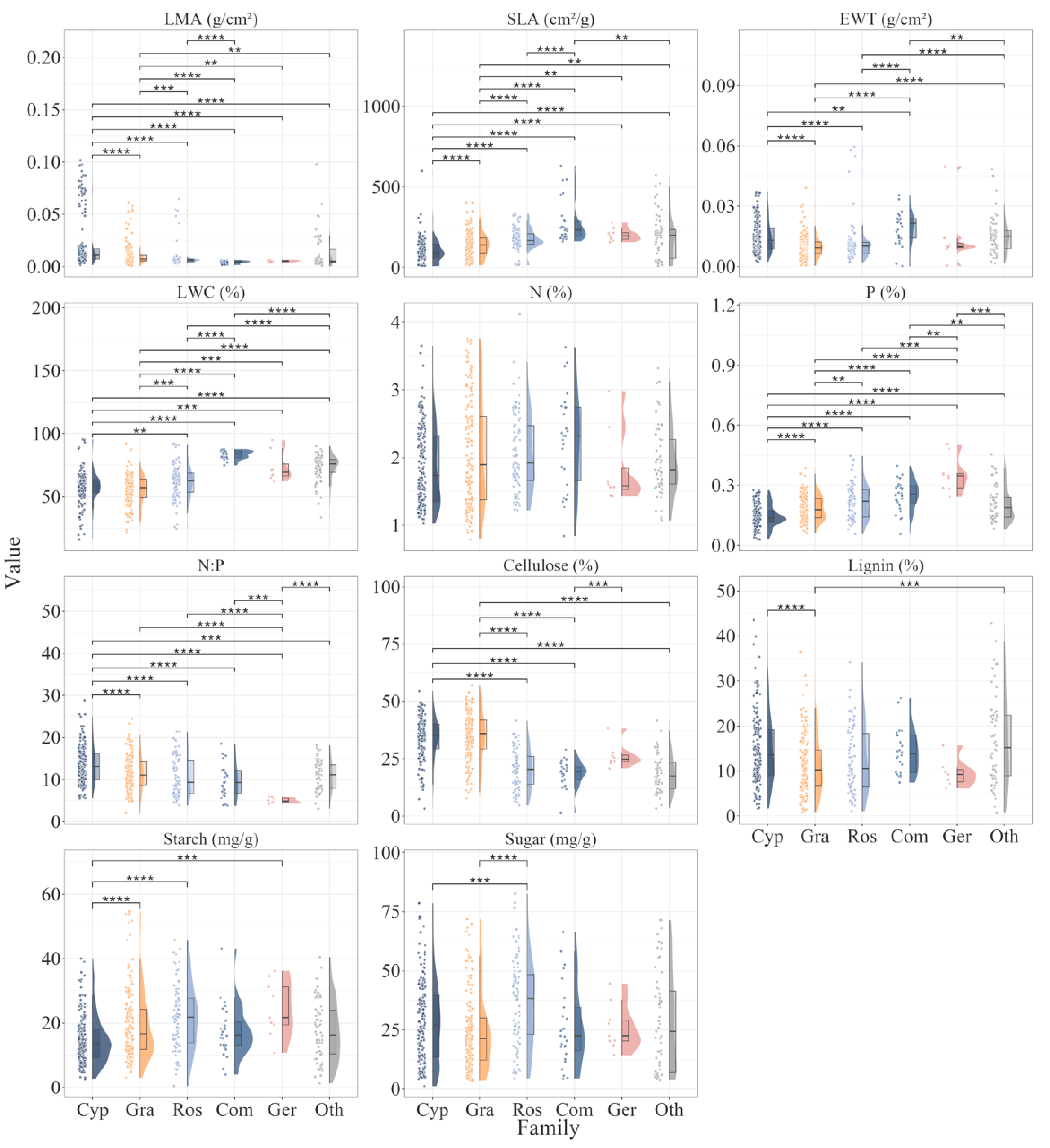
Figure 3.
The PLSR models with different sample sizes (S40: 40 samples, S80: 80 samples, S120: 120 samples, S160: 160 samples, S200: 200 samples, S240: 240 samples, box plot is validation R2, line chart is RRMSE, LWC represents leaf water content, SLA represents specific leaf area, LMA represents leaf mass per area, and EWT represents equivalent water thickness).
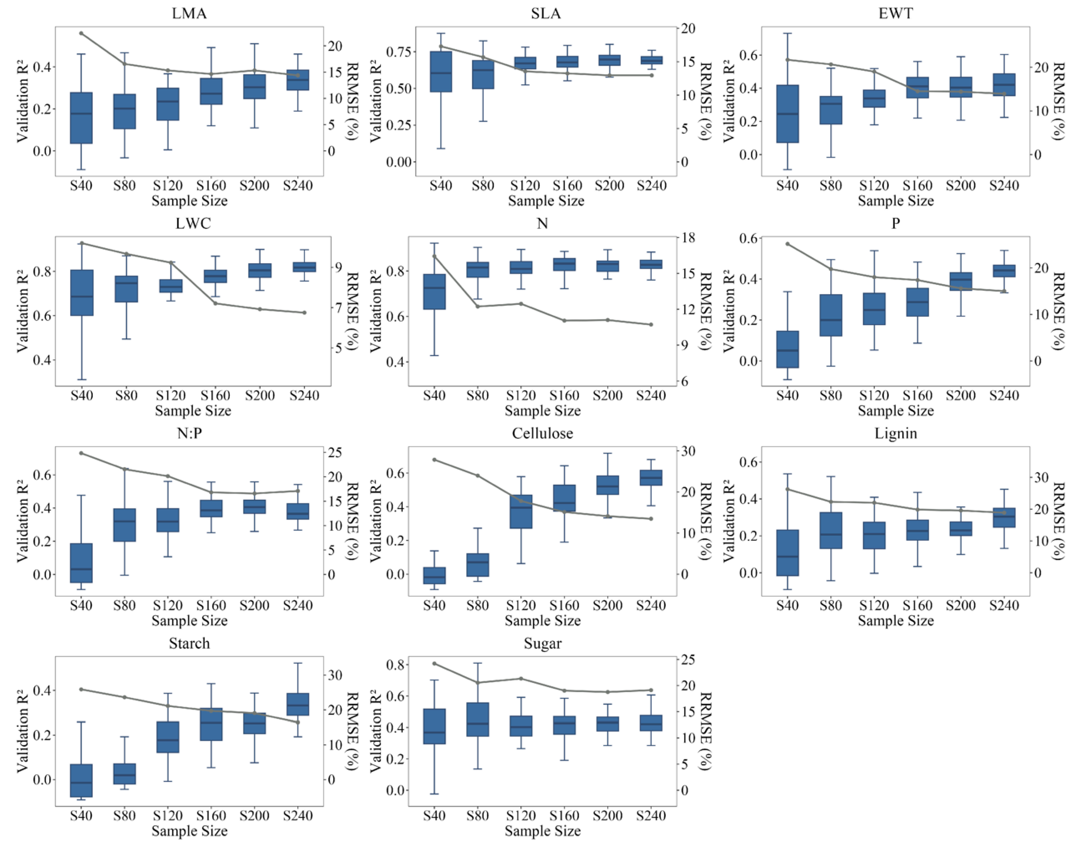
Figure 4.
Comparison of validation model accuracy in spectral inversion traits for different species combinations (AF: All-families, DF: Dominant-families, CG: Cyperaceae-Gramineae, NC: Non- Cyperaceae, CY: Cyperaceae).
Figure 4.
Comparison of validation model accuracy in spectral inversion traits for different species combinations (AF: All-families, DF: Dominant-families, CG: Cyperaceae-Gramineae, NC: Non- Cyperaceae, CY: Cyperaceae).
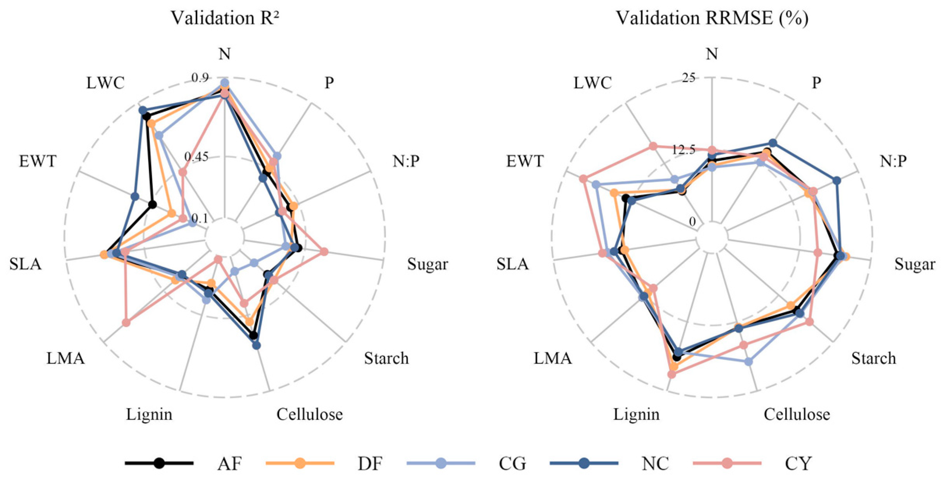
Figure 5.
Wilcoxon analysis of validation model accuracy for spectral inversion of leaf traits with different species combinations (AF: All-families, DF: Dominant-families, CG: Cyperaceae-Gramineae, NC: Non- Cyperaceae, CY: Cyperaceae. ns: p > 0.05, *: 0.01 < p < 0.05, **: p < 0.01, ***: p < 0.001,****: p < 0.0001).
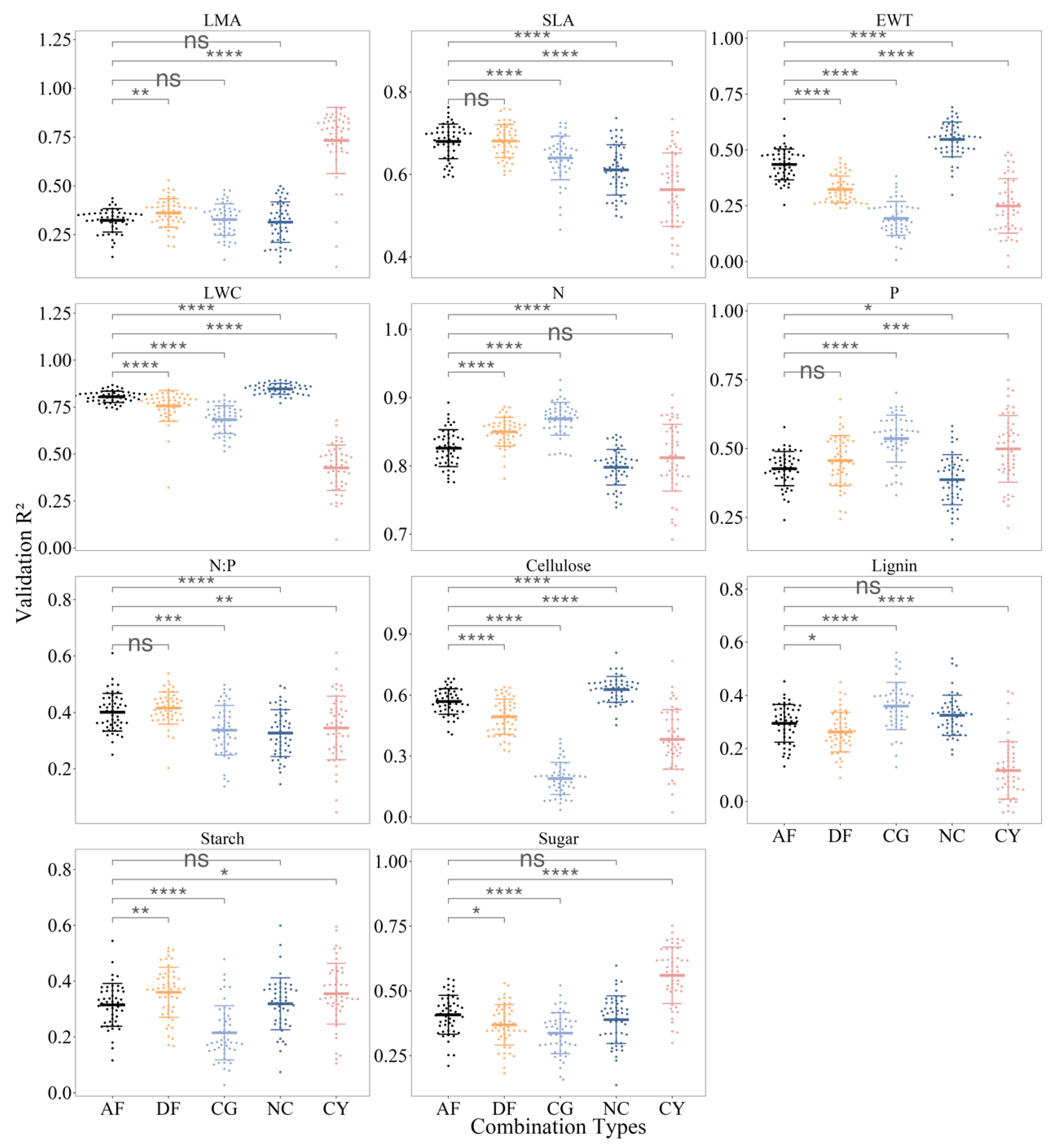
Figure 6.
Explained proportion of sample size and species combinations to spectral inversion of leaf traits (SC: species combinations, SS: sample size).
Figure 6.
Explained proportion of sample size and species combinations to spectral inversion of leaf traits (SC: species combinations, SS: sample size).
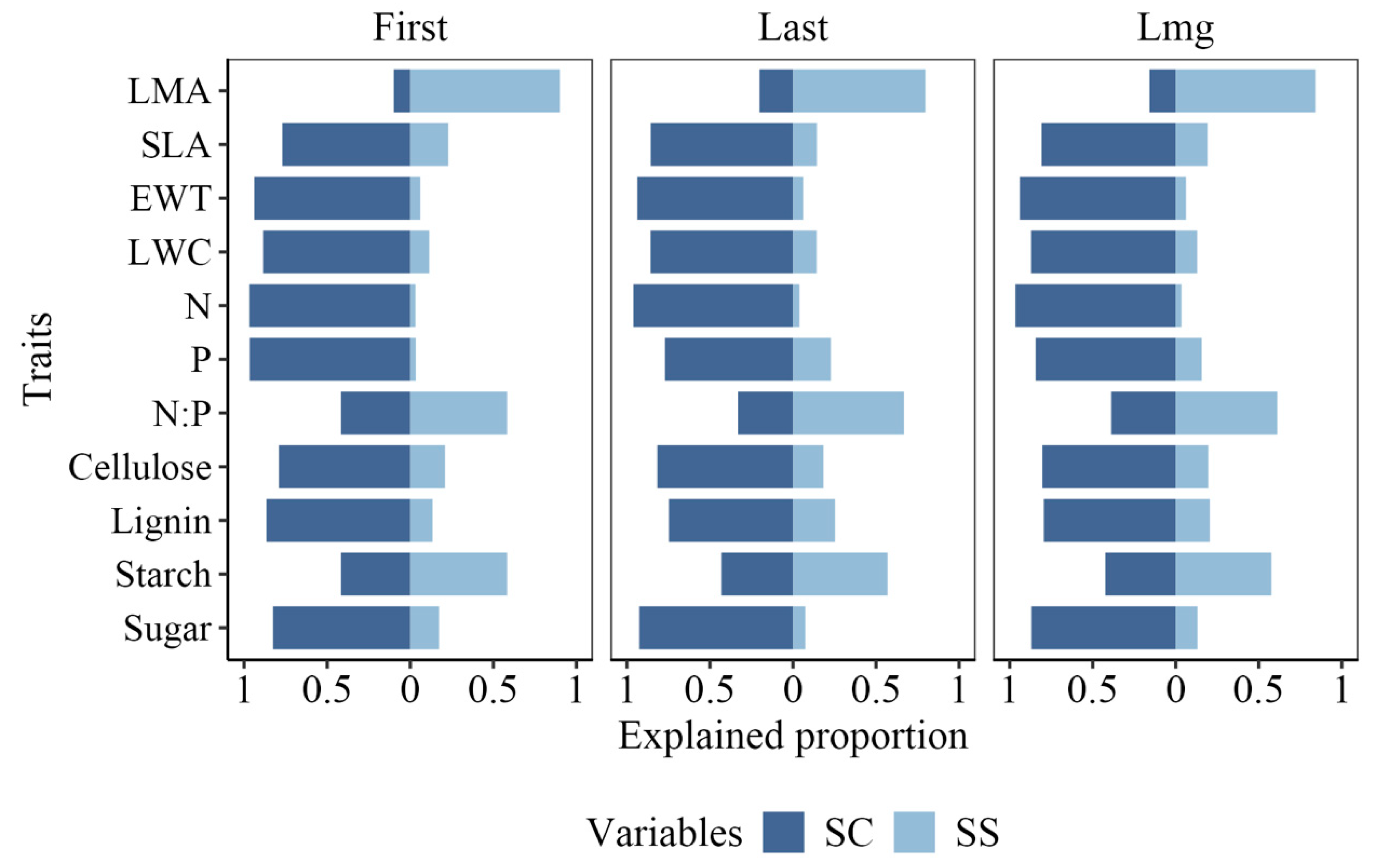

Table 1.
Sample sites and total samples for different plant families.
| XBHNNR | SHPNNR | SJNNR | YHNNR | Total | |
|---|---|---|---|---|---|
| Cyperaceae | 21 | 12 | 94 | 10 | 137 |
| Gramineae | 17 | 44 | 75 | 6 | 142 |
| Geraniaceae | 7 | / | / | / | 7 |
| Compositae | 9 | 3 | 5 | 1 | 18 |
| Rosaceae | 23 | / | 37 | 5 | 65 |
| Others | 6 | 7 | 38 | / | 51 |
| Total | 83 | 66 | 249 | 22 | 420 |
Disclaimer/Publisher’s Note: The statements, opinions and data contained in all publications are solely those of the individual author(s) and contributor(s) and not of MDPI and/or the editor(s). MDPI and/or the editor(s) disclaim responsibility for any injury to people or property resulting from any ideas, methods, instructions or products referred to in the content. |
© 2025 by the authors. Licensee MDPI, Basel, Switzerland. This article is an open access article distributed under the terms and conditions of the Creative Commons Attribution (CC BY) license (http://creativecommons.org/licenses/by/4.0/).
Copyright: This open access article is published under a Creative Commons CC BY 4.0 license, which permit the free download, distribution, and reuse, provided that the author and preprint are cited in any reuse.


