Submitted:
17 March 2025
Posted:
18 March 2025
You are already at the latest version
Abstract
The 210Pb-based dating method provides absolute ages determination in recent aquatic sediments at centennial scales. It is widely used to support a large variety of environmental studies. However, any empirical data set is compatible with an infinite number of chronologies that need to be constrained by a series of assumptions (models) on the particular sedimentary conditions of the studied environment, and validated with independent chronostratigraphic markers. During five decades, about thirty models have been developed to cope with the wide diversity of natural conditions, a good number of them appearing in recent years, along with new concepts such as model errors, attractors for χ-mapping, or kinetic reactive transport, which have changed common views and practices. This paper aims to present a comprehensive review of this dating method to provide to final users updated tools and a renewed understanding to improve the reliability of their applications. Models are classified in terms of their assumptions on the sedimentary systems, which are better understood from a revisited theory of early compaction and the description of the microcosms of saturated porous media, where composite fluxes of tracers undergo different deposition pathways in terms of physical and kinetic reactive transport. The article reviews empirical evidence on the natural variability in mass flows and initial activity concentrations. Some models allow analytical solutions, while others require numerical techniques. The review is illustrated with examples from real case studies.
Keywords:
210Pb-dating
; 210Pb-based models
; sedimentation rates
; polyphasic porous media
; aquatic environments
1. Introduction
The radiometric dating has represented a revolutionary contribution to the study of sedimentary processes, being the only technique of general applicability that can provide an absolute age determination (Carroll and Lerche, 2003). The method based on the natural radionuclide 210Pb is widely used to determine ages and sedimentation rates in the past 100 to 150 years, with about 4000 scientific documents in Scopus (search criteria ‘210Pb and sediment’). 210Pb- based chronologies can support a wide diversity of studies, including, among others, decoding past natural and anthropogenic impacts in sedimentary conditions (e.g., Lu and Matsumoto, 2005; Trabelsi et al., 2012; Begy et al., 2018; Chen, et al., 2019), the history of anthropogenic pollutants (e.g., Kirwan and Megonigal, 2013; Ontiveros-Cuadras et al., 2024), quantification of carbon sequestration capacity of vegetated coastal sediments (e.g., Kristensen et al., 2008; Marchand, 2017), or studying the interplay of global sea level rise and accretion rate of saltmarshes sediments (e.g., Madsen et al., 2007; Gore et al., 2024).
During the past three decades, a gap has emerged between method developers and end users. Most studies use only three of the approximately 30 models developed to address the wide diversity of sedimentary systems, and often apply them beyond their intended use.
Far of being a closed problem, there has been an intense activity during recent years around the fundamentals of the technique, with the rise of new models such as TERESA, PLUM, RUS2023 and the family of χ-mapping models, as reviewed latter in this work. Lessons learnt have shown some shocking results. Thus, any empirical data set (a mass depth profile of 210Pb and 226Ra) is compatible with an infinite number of different mathematically exact solutions for the chronology (e.g., Robbins, 1978; Abril, 2015).
The chronology must be constrained by a set of assumptions on the sedimentary conditions, called a 210Pb-based model. It could be though that different assumptions should produce different chronologies, reducing the problem to find the right assumptions for each specific scenario. However, different models can often produce very close chronologies (eg, Abril, 2020). This leads to the concept of model errors (deviations from model output and the true solution due to a partial or null accomplishment of the model assumptions). Their quantification in varved and synthetic cores has revealed that the model records of sedimentation rates, profusely used in literature for tracking past environmental changes, are undermined by large model errors, which makes futile their use for this goal, while the proper magnitude, the initial activity concentrations, never captured our attention. It is also surprising that the model solution that best fits the empirical profile does not necessarily lead to the most likely chronology, as has been shown with the study of the attractors (Abril, 2023d).
The 210Pb dating method needs the support of independent chronostratigraphic markers, and bomb-fallout radionuclides such as 137Cs, 241Am and 239+240Pu have been profusely used for this goal. A large set of additional data can support the holistic analysis of a sediment core. Thus, sediment dating becomes only a part of a more general and interesting problem consisting of understanding the particular sedimentary conditions and processes that govern the environmental behaviour of radionuclides and anthropogenic pollutants. The application of reactive kinetic transport models for the upper regions of aquatic sediments has changed our view on these processes (Abril and Barros, 2022; Abril, 2024).
This work aims to present a comprehensive review of about 30 different 210Pb dating models developed during the last five decades, with a classification based on the specific sedimentary conditions they represent. For this end, it is necessary to review the main features of the porous medium of sediments and on the kinetic reactive transport of different radiotracers to understand under which circumstances it can be considered as a continuous medium or a polyphasic one. Radiotracers may reach the SWI in dissolved form or attached to a wide diversity of carriers with diverse provenances and path histories. Depending on the scenario, different contributions may govern this composite nature of the fluxes.
Due to the large number of models considered in this work, they cannot be presented in full mathematical detail. It would be advisable for the reader to be already familiarised with at least some of the simpler classical models. There are some reviews that can be particularly helpful for beginners (see, e.g., Sanchez-Cabeza and Ruiz-Fernández, 2012) and some essential references such as Robbins (1978) and Appleby (1998). Although not necessarily at a fundamental level, it would be helpful to get a general idea of other 210Pb-based models used in the scientific literature. Some helpful review papers can be found, among others, in Mabit et al. (2014) and Arias-Ortiz et al. (2018). In this work, the reader will also find references from the scientific literature for each specific model mentioned.
Not treated here are the tasks related to the sampling of sediment cores, the sample treatment, and the nuclear techniques for measuring the radionuclides of interest. For the first topics, the reader is addressed to the IAEA TEC-DOC 1360 (IAEA, 2003). A comparative study of alternative methods for 210Pb determination in environmental samples can be found in Zaborska et al. (2007) and Cuesta et al. (2022), among others.
2. 210Pb Cycling in Nature and the Rise of Dating Models
Aquatic sediments accrete with mass flows from a diversity of provenances that contribute with varying intensities over time. 210Pb (T1/2 = 22.3 yr.) is generated in the radioactive decay chain from 226Ra (T1/2 = 1600 yr.), 222Rn being the radioisotope in between with the longest half-live (T1 / 2 = 3.82 days). Measuring 226Ra and 210Pb mass activity concentrations in the surficial layers of sediments uses to reveal a lack of secular equilibrium, with 210Pb being in excess with respect to 226Ra. The amount in excess is denoted hereafter as 210Pbexc (following Krishnaswamy et al., 1971), while the amount that equates the mass activity concentration of 226Ra is referred to as supported 210Pb, and denoted as 210Pbs.
210Pbexc ultimately comes from the 222Rn exhaled by the continental crust and dispersed in the atmosphere where it decays to 210Pb, which is attached to the surfaces of aerosols and dust particles. It is scavenged by wet and dry fallout and accumulates in the surface layers of soils and sediments. The 210Pb fallout rate is locally governed by wet deposition and it largely varies over time in the range from hours to years, with annual fallout fluxes that at a global scale ranging from 0.1 to 360 Bq m-2y-1 (Mabit et al., 2014).
In aquatic sediments, the meteoric 210Pb that reaches the sediment-water interface (SWI) has met the particulate matter of the mass flows at different stages of their paths from their provenances. Thus, the 210Pbexc flux at the SWI is conceptually different from the atmospheric deposition in the area, taking different values and with a temporal variability driven by different factors. The discrete slicing of the sediment cores in environmental studies implies a temporal discretization that, depending on the sedimentation rates, may range from a few months to a few years. Thus, the physically significant values of the 210Pbexc flux at the SWI must refer to these time intervals. Independently of its path history, the mass activity concentration of 210Pb found in excess in the material accreting on the sediment is referred to as the initial activity concentration, and denoted as
.
Aquatic sediments are porous media that remain permanently saturated with water, so the diffusion and exhalation of 222Rn is generally negligible. Thus, once meteoric 210Pb has been incorporated into the sediments, the amount of 210Pbexc decreases with time by radioactive decay, and in some scenarios it can also undergo some redistribution processes. These features have inspired the 210Pb dating method, initially proposed by Goldberg (1963) for dating glacier ice. It was first applied to lacustrine sediments by Krishnaswamy et al. (1971) and to marine sediments by Koide et al. (1972).
The first models used very simple assumptions on the sedimentary conditions. Thus, Krishnaswamy et al. (1971) presented a linear fit for the logarithmic plot of 210Pbexc versus depth in two sediment cores, which they interpreted with the assumptions of constant 210Pbexc flux, constant sedimentation rate (CFCS model), and uniform bulk density. A similar analysis was used by Koide et al. (1972) for a varved marine sediment core, demonstrating the use of the 210Pb method with the independent chronology from varves.
As the application cases to other lacustrine and marine environments increased, certain limitations were found in the above approach, leading to the rise of new models considering temporal variability in fluxes, mixing, and diffusion. Only six years after the paper by Koide et al. (1972), Robbins (1978) presented a comprehensive review of the state of the art and stated the pillars of the 210Pb dating method. It is worth summarising the following points:
(i) The mass depth scale should be used in the models instead of the metric depth to account for compaction and shortening.
(ii) There are an infinite number of chronologies being the solution of any given empirical 210Pbexc profile, so assumptions on the fluxes of matter and 210Pbexc are necessary to constrain a solution.
(iii) The author presented analytical solutions for models assuming a constant flux (CF), a constant flux with a constant sedimentation rate (CFCS), including its piecewise version, a constant initial concentration (CIC), and a differential equation for a model with the 210Pbexc flux being a linear function of the sedimentation rate.
(iv) Solutions were provided for a family of models considering diffusion, raising as particular solutions of an advection-diffusion equation written in terms of metric depths (previously used by Guinasso and Schink, 1975).
The work included applications to real cores and identified special cases with 210Pbexc profiles showing disruptions due to slump events. It is worth noting the limitation in the above work of using the diagenetic equations by Berner (1971, 1982), which were latter revisited by Abril (2003a).
In the same year, Appleby and Olfield (1978) published their version of the CF model, named as the constant rate of supply (CRS) model. Appleby et al. (1979) applied this model to three varved sediments from Finland, with a reasonable agreement between the model and varve chronologies, while the CIC model failed in two cases. It is worth noting that the CRS model was used here with the addition of a reference date (the varve date of the deepest sediment slice), so that the CRS chronology necessarily fits the varve chronology at this point and at the SWI, and captures the main value of the sedimentation rate. This is known as the reference-date method (Appleby, 2001; Abril, 2019), which is different from the basic and widely used version of the model when the age of the deepest slice is unknown.
The CRS model has a simple analytical formulation and apparently powerful outputs: the chronology and the history of the sedimentation rates. This explains its popularity. By the use, the model assumptions seem to have acquired the category of physical principles, being applied, without adaptation to sedimentary scenarios where the assumptions do not hold.
Some authors, such as Smith (2001), with outstanding contributions to the development of the 210Pb dating technique, claimed that it should be mandatory that any 210Pb-based chronology be validated by independent chronostratigraphic markers. For this end, the artificial 137Cs, 241Am and 239+240Pu, with characteristic peaks in their history of atmospheric deposition, are being profusely used.
Very soon, it was noticed that mixing could translocate the position of the peaks of 137Cs (e.g., Robbins and Edgington, 1975), while diffusion and mixing affect differently to high-particle-reactive radionuclides, such as 239+240Pu and 210Pb. To distinguish post-depositional mixing from pre-depositional processes it was necessary the development of specific models for these man-made radionuclides (e.g., Robbins et al., 2000). A more recent view explains the effects attributed in some cases to diffusion, as result of the kinetic reactive transport of radionuclides through the d pore fluid (Abril and Barros, 2022).
3. The Porous Media of Recent Sediments
3.1. Bulk Density and Early Compaction
Due to natural compaction, and the shortening during coring, storage, and extrusion, the metric scale does not represent the undisturbed conditions. However, the mass-depth scale remains invariant under the above processes, and the bulk density profiles still preserve information on early compaction.
The dry-bulk density is defined as the mass of dry solids divided by the total volume of the wet sample. There are two basic methodologies for estimating bulk density: i) Method I involves direct measurements of dry mass and bulk volume; ii) method II involves other index properties and a conceptual model of the porous media.
Method I uses a sediment sample of well-known unperturbed bulk volume, V, (usually from a known cross-sectional area and thickness), and measures (by weight) its mass (wet sediment),
. Alternatively, the wet volume can be estimated from the volume of water displaced by the wet sediment. The dry sample weight can be determined by drying the same sample in a freeze-dryer or in an oven at 110° ± 0.5°C, for 24 h (Dadey et al., 1992), although in the scientific literature one can find a large diversity of drying protocols. The remaining mass,
, corresponds to the dry solids (along with the precipitated salts from the interstitial solution). Then, the bulk density, ρb, is
Equation 1 provides a good estimate for freshwater environments, but for saline pore fluids must be corrected by the amount of precipitated salts (Dadey et al., 1992; Iurian et al. 2021):
where * denotes salt-corrected values and is the fraction (in weight) of salts in the pore fluid.
Shear stress during sediment coring and extrusion can promote vertical displacement of sediments adjacent to the internal surface of the sampler. This perturbation can be minimised in the lab by using a sub-sampler cylinder of thin wall and wide cross section.
Method II estimates the bulk volume from a ‘sediment model’ with several constituents. Its simplest version considers only two constituents: solids and pore water. The weight fraction of water is . The bulk density can be estimated (assuming uniform values for the density of solids,, and water, , and additivity of partial volumes) as
The density of solids, , can be measured by (gas) picnometer for each sediment slice, although the most common approach assumes a reference value, typically =2.65 gˑcm-3, the density of quartz and clay minerals. Equation 3 needs a correction for saline pore fluids (as in Eq. 2). Note that corrections by precipitated salts must be consistently applied to bulk densities and to radionuclide mass activity concentrations.
Method II can be refined by accounting for the organic matter content (usually determined by LOI). This is particularly important for vegetated coastal sediments, where the organic matter content can exceed 50% of the sediment dry weight. However, here the assumption of additivity of partial volumes is questionable.
Comparison between procedures I and II is recommended. Under field and/or laboratory conditions, some sediments can be partially unsaturated, and the volume of pores occupied by air produce the failure of the second method. The comparison allows estimating such a void volume, which provides some insight into the sediment structure close to the SWI. A high LOI value due to plant roots also challenges the two-constituent conceptual model, since a significant fraction of the water lost by evaporation is not pore water but vegetal tissue water. An example of a polyphasic model of porous media including plant roots in a vegetated soil can be seen in Taieb Errahmani et al. (2022).
The mass depth m(z) is the dry mass per unit area accumulated from the SWI until the sediment horizon that at the slicing operation is at depth z, and it can be estimated from the bulk density:
In practice, the integral is replaced by a discrete summation of all the sediment slices comprised from the SWI to depth z.
In sediments that met the model of a two-phase porous medium, steady-state bulk density profiles are produced by gravitationally driven early compaction (solids tend to replace the pore water below them) and they approach the mathematical expression:
where γ is a scaling factor and is the asymptotic value for bulk density, referred to as the early-compaction limit; is its value at the SWI and . Some examples are shown in Figure 1 (cases A and B).
In the theory for early diagenesis, Berner (1980) inconsistently used an advection-diffusion equation for the mass conservation of solids in terms of the bulk density. The revised theory for early compaction (Abril, 2003a) introduced a specific potential energy for solid particles, , which decreases when the water pores are occupied by solids. It is defined as energy per unit weight and referred to as the compaction potential. From a reference frame anchored at the SWI of a sediment that accretes with a metric velocity v, the mass flow of solids through a sediment horizon at depth z is , where is the relative velocity at which solids displace due to early compaction.
is a conductivity function that decreases with depth and vanishes at the early compaction limit (Abril, 2011). The continuity equation that expresses the mass conservation of solids then writes:
As at the early-compaction limit q vanishes,
The steady-state solution of Eq. 7 implies that the mass flow is uniform through the sediment column. At the SWI corresponds to the mass sediment accumulation rate, referred to as SAR.
It is worth noting that in most applications, we usually report mass flow or sediment accumulation rates, w, but in some cases, such as those when the major concern is their comparison with the rise in sea level, the relevant magnitude is the linear accretion rate of the SWI, v, given by Eq. 8 (many works incorrectly use ).
Abril (2011) relates the gradient of the compaction potential with the buoyancy ( ) as . To obtain Eq. 5 as the steady-state solution of Eq. 7, it is necessary to explicitly note that conductivity decreases with depth, its rate of change being proportional to the default bulk density, defined as : . is a parameter that encloses information on the granulometry of the solids, being a constant when the latter is uniform through the core. Numerical solutions of the above equations for early compaction under varying sedimentary conditions can be found in Abril (2011).
The above Eqs. 6-9 refer to sediment under natural conditions, while the plot of Figure 1 captures the situation after coring, storage, extrusion, and slicing the core. However, Figure 1 provides information on the early-compaction limit, useful for reporting metric accretion rates. Deviations from the steady-state trend can reveal some abrupt changes in environmental conditions, some of them likely related to episodic sedimentation of coarser materials, upslope soils, or erosive events, among others, such as Example C in Figure 1 (see details in Abril et al., 2018).
Intuitively, early compaction is driven by the gravitational forcing and the perturbations (micro-earthquakes, pressure waves, bottom search stress, etc.) that promote the reallocation of solids and pore fluid. Early compaction can work with a progressive decrease of the pore space, but also with the relative downward transport of colloids and very small size fractions. However, this view does not apply in vegetated sediments, where rhizospheres represent a distinct phase with belowground production and decay, conform the sediment structure, and have a distinct advection relative to the mineral phase. However, some basic features relative to an early compaction limit below the rhizospheres still hold (see Iurian et al., 2021).
3.2. The Continuity Equation for a Particle-Bound Radiotracer in Porous and Accreting Sediments Under Early Compaction
For radionuclides of interest in radiometric dating (210Pb, 137Cs, 241Am, 239+240Pu), the distribution or partition coefficient, kd (defined as the dimensionless ratio at equilibrium between mass concentrations in solids and in solution), is of the order of 103 to 107 (IAEA, 2010). Consequently, although sediments are saturated porous media, almost 100% of these radionuclides are expected to be bound to the solid phase at equilibrium. This justifies the common approach of considering sediments as continuous media. The continuity equation, in terms of the metric depth, , is (Abril, 2003a):
where is the radioactive decay constant, is the mass activity concentration of the studied radiotracer, and is a diffusion coefficient. By using Eq. 7 and that , Eq. 9 can be written in terms of mass depth, :
where is an effective coefficient for diffusion, and w denotes SAR. Note that and are functions of and time. Solving Eq. (10) requires the provision of initial and boundary conditions. At the SWI (m = 0), the continuity of fluxes is commonly imposed as a boundary condition:
where is the flux of tracer at the SWI. This is, the time series of 210Pbexc fluxes and SARs must be introduced as input information, as well as the particular parameterization of . At the bottom boundary, for .
Note that Eqs. 10-11 apply for tracers bound to particles of solids; thus, the diffusion requires a downward and upwards displacement of solids with a net null mass flow. The upward displacement is opposite to the gravitational forcing and requires the existence of a forcing agent. Bioturbation can provide such a forcing (e.g., Robbins and Edgington, 1975; Robbins, 1978). Spatial variability of mass flow through the sediment cross section results in a tiny diffusion term, similar to turbulent diffusion in the Reynold equations for fluids (Abril, 2011), but it can be neglected in most cases. When takes very high values in a top zone of the sediment and vanishes below, the effect in is usually referred to as a mixing. The tidal cycles of resupension and deposition in some coastal sediments can result in a mixed surface layer that can be formally described by a depth-dependent . Depth distributions of radiotracers promoted by kinetic reactive transport have been described by depth-dependent , but this description fails for cores sampled at the same site after a elapsed time, as discussed further below.
3.3. Composite Fluxes of Tracers and Kinetic Reactive Transport in the Porous Media of Aquatic Sediments
Figure 2 shows a sketch illustrating the physical environment of the SWI, which is an irregular, rugose, and porous interface. Stacked solids of varying sizes and mineralogical nature conform to the structure of the porous medium, with the pore spaces occupied by water. Trace elements reaching the SWI can be associated to a wide diversity of carriers (large structural particles, fine grained and colloidal fractions, organic compounds, etc.), which may have reversible and irreversibly bound components, and they can also be present as free ions into solution. A fraction of the free surface of solids remains inaccessible to the pore water due to stacking. Solid particles have rugose and porous surfaces where uncompensated electric charges and more specific reaction sites are distributed (Eisma, 1993). The uptake of trace elements from the dissolved phase is a kinetic process that can be described by box models with a set of parallel and consecutive reversible reactions, along with some irreversible components (Barros and Abril, 2008).
Different carriers show different depositional patterns; those bound to structural particles are ideally deposited at the top region of the SWI, while the mobile fractions (dissolved and colloidal) are transported through the pore fluid. Even for weakly particle-reactive radionuclides, such as 137Cs or 7Be, the typical percolation velocities do not result in significant penetration depths; and the same is true for molecular diffusion (Abril and Barros, 2022). However, in those ‘energetic’ systems where the overlying water column has a noticeable eddy diffusivity (e.g., because of tidal or wind-driven currents), this does not drop to zero at the SWI, but perturbs the pore space, progressively vanishing with depth. The interplay of the kinetic uptake with this transitional eddy diffusivity can result in noticeable penetration depths for mobile radionuclides, while those others highly particle-reactive, such as Pb and Pu isotopes, are retained in the first few millimetres of the sediment column (Abril and Barros, 2022; Abril, 2024).
Shortly after the peak in atmospheric bomb-fallout, or after the Chernobyl accident, artificial Cs isotopes reached the SWI mostly in mobile form, reaching penetration depths of up to more than 10 cm in some energetic sedimentary systems while in others, free of eddy diffusivity, they were trapped in a very thin surface layer. In the former systems, Cs isotopes continued reaching the SWI but now bound to solids of different provenances and undergoing ideal deposition (Abril and Barros, 2022). In general, the mobility downcore of a fraction of the input tracer may coexist with the ideal deposition of another fraction bound to structural particles.
241Am, Pu isotopes and 210Pbexc, even in cases where a fraction of their inputs may be in dissolved form and transitional eddy diffusivity is present, do not show any significant depth penetration. Exceptions can be made in those cases where the colloidal fraction is particularly relevant.
The set of governing differential equations and the application of the kinetic reactive transport models in real cases for 137Cs, 7Be, 210Pb, 239+240Pu and 236U can be found in Abril and Barros (2022) and Abril (2024).
Figure 2 also highlights the composite nature of the 10Pbexc fluxes. Different contributions may have varying weights as responses to seasonal changes, episodic events, and human impacts. When the particle-bound fraction of the 210Pbexc inputs is dominant, intensification in mass flow can result in an increase in global 210Pbexc flux. This must be understood in terms of statistical correlation more than in terms of a physical law, since the intensification of the mass flows may involve varying weights of components with different provenances, resulting in different aggregated .
Abril and Brunskill (2014) reported the reconstructed palaeorecords of SARs, and 210Pbexc fluxes in varved sediments from a variety of lacustrine, riverine, and marine environments. They found large but independent variability in SARs and initial activity concentrations (roughly approached by normal or log-normal distributions), resulting in a positive correlation of 210Pbexc fluxes and SARs (Figure 3).
4. The Empirical Dataset
For a sediment core that has been sliced into n sections, the 210Pb method needs n pairs of values of 210Pbexc mass activity concentrations with their analytical uncertainties, and the mass thickness of each slice (. This will be referred to as the primary data. The mass thickness allows for the construction of the mass depth scale, it is needed for estimating the inventories required in some models, and relates with the bulk density of each slice.
Independent chronostratigraphic markers must be used when possible; examples are artificial 137Cs, 241Am, and 239+240Pu, tephras, pollen markers, anthropogenic pollutants with known deposition histories, etc. They can serve for validating the 210Pb-based chronology, or as integral part of the method.
As common analytical methods involve gamma measurements, other γ-emitter radionuclides can be recorded simultaneously. Thus, the cosmogenic 7Be, when found in the upper layer, serves as a quality control of a coring procedure without loss of the upper material. When found distributed in depth, it informs on non-ideal deposition, either for transitional eddy diffusivity or for the lack of definition of the SWI, what alerts of similar effects with 137Cs in both cases, and with 210Pbexc in the latter. 226Ra serves to estimate the supported fraction of the total of 210Pb, but its depth profile is useful in identifying changes in sedimentary conditions. This last can be reinforced when such changes simultaneously occur in the depth profiles of 40K and 228Ra (e.g., see Abril et al., 2018).
For vegetated sediments, the analysis of LOI and in situ concentration ratios must be considered (see Iurian et al. 2021).
Granulometry, mineralogy, magnetic properties, concentrations of trace metals and other anthropogenic pollutants, etc., conform a wide set of data for the holistic analysis of sediment cores, along with the geochronological data, and can support the best model choice. This work focusses on the dating models built from the primary data for 210Pbexc and the artificial radionuclides that can support the chronology.
In this work, the use of the models will be illustrated with real cases from the literature. The raw data sets needed are available in the referenced papers, so they are not replicated here.
5. Overview of 210Pb-Based Dating Models
Analytical solutions of Eq. (10) can be found only in some simple cases, but numerical solutions are always possible. The solution is unique for each particular setting of all the required input data. However, the reverse is not true. 210Pb-based models can be seen as particular solutions of Eq. 10, but they can also be directly derived from their basic assumptions as originally formulated.
A summary of the models developed during the last five decades is presented in Figure 4. The first and most populated group of models share the following assumptions: i) Tracers are particle-bound, which allows for the simplification of considering a continuous medium characterised by its bulk density. ii) For 210Pbexc, penetration depths are negligible, so the assumption of ideal boundary conditions (continuity of fluxes at the SWI) can be adopted. iii) There is no postdepositional redistribution ( in Eq. 10). Implicitly, the continuity of the sedimentary sequence is also assumed, which is not disrupted by erosion nor by episodic slump events. These assumptions may hold in a large proportion of lacustrine systems and marine basins. Exceptions are sediments with bioturbation and sites with energetic hydrodynamics (with wind or tidal forcing) that may result in a mixed sediment layer. In deep-sea sediments uniform diffusion has been considered in several studies, the reason being their common very low sedimentation rates, so that tiny physical redistribution processes may gain relevance comparatively.
Within the above group of models, a first distinction is whether se sedimentary conditions prevail for the entire range of the chronology of the core, or whether there are two or more transects with distinct conditions. This can be elucidated from a cluster analysis (Abril, 2019), as illustrated in Figure 5. Briefly, the logarithmic plot Ln[A(m)] can reveal slope and/or jump discontinuities, in which case a piecewise analysis must be conducted. In the absence of such discontinuities, the simplest version of the models can be used.
With these assumptions, the boundary condition writes: . A first group of models assumes the flux to be constant in time, a second group assume a constant sedimentation rate, , a third group considers a constant initial activity concentration, , while a four group considers the three magnitudes varying with time.
After getting familiar with the above set of dating models, it is possible to discuss model errors and studying the methods for extending their application to multitransect problems.
Validation of the chronology with independent time markers is necessary in all the cases. However, some models can use the reference dates provided by the time markers as an integral part of the model formulation, rather than as an external validation.
The use of artificial radionuclides such as 137Cs and Pu isotopes as time markers is not so straightforward since their fluxes reaching the SWI may noticeably differ from the histories of their atmospheric deposition. Thus, Figure 4 considers some specific models for these predepositional processes.
Another group of 210Pb-dating models accounts for diffusion or mixing but still keeping the assumption of a continuous medium and the continuity of fluxes at the SWI. The simple case of steady-state solutions under constant fluxes and SARs allows for analytical solutions. The man-made 137Cs is particularly prone to undergo post-depositional redistribution, which complicates its use as a time mark. Although these processes will be better understood from the kinetic reactive transport, there are a series of models accounting for diffusion and mixing that can be adapted for man-made radionuclides with their time-dependent fluxes.
Numerical solutions of Eq. 10 can face any kind of problems with depth-dependent diffusion and temporal variability in fluxes and SARs, when keeping the assumption of a continuous medium and the boundary condition of Eq. 11.
The assumption of ideal deposition at the SWI can be broken when a fraction of the fluxes undergoes a fast depth penetration. However, this problem can be treated keeping the formalism of a continuous medium by introducing a depth-dependent source term. This is the NDI model considered in Figure 4, as a transition to models that surpass the assumption of a continuous medium. Within them, Figure 4 considers models for the reactive transport of tracers into solution, but this can be faced with the approach of a local equilibrium, described by a partitioning coefficient, or by solving the kinetics of the uptake.
The assumption of a continuous medium also breaks down in vegetated sediments, where the rhizospheres represent a distinct phase, with achronical below-ground production and decay, a distinct uptake of tracers and a quite different physical transport. Faceting this problem requires updating both the analytical methods and the models.
The above classification does not encompass the full diversity of sedimentary conditions that have been studied in the scientific literature. Thus, a group of some special cases will be considered in this work.
6. Models for Continuous Media, Ideal Deposition, and Non-Post-Depositional Redistribution
6.1. A Single Transect in the Ln[A(m)] Plot
6.1.1. Models Assuming a Constant Flux
CFCS model
Within the models assuming a constant flux, additional assumptions are still necessary. The CFCS model assumes a constant SAR, which implies an also constant , allowing for the analytical formulation:
A least squares fit to the empirical data (, ) allows solving and and then the flux ; the chronology being . However, there are different possibilities to perform the fit others that the least squares (e.g., weighted fit by , minimum distance, etc.).
χ-CFCS model
The χ-mapping version of the CFCS model uses a numerical technique that tests a very large number of possible pairs of values for and to find the pair that minimised a χ2 function (see details in Abril 2023c).
CF (CRS) model
The constant flux model (CF in the formulation by Robbins, 1978; and CRS in the equivalent version by Appleby and Oldfield, 1978) assumes a steady-state total inventory below the SWI. The inventory below the sediment horizon at mass depth m is , and the total inventory corresponds to . In practice, the integral is replaced by a discrete summation using the empirical data (, ). This assumption allows for the analytical solution for the chronology:
The SAR history can be obtained from and the above chronology, although alternative analytical formulations can be handled (see Abril 2023c). Note that steady-state inventories are not met, even under conditions of a constant flux, in sedimentary systems younger than a century, as may be the case of some reservoirs and harbours.
In some cases, the core length is not long enough to recover the total inventory, which prevents the application of the CF model. However, when the trend line of in the deepest section of the core is well defined, it is possible to use the local value of SAR (inferred from a CFCS model) to extrapolate the missing tail and estimate in this way the missing part of the inventory. This is the reference-SAR method, which can be considered as a version of the CF (or CRS) model that uses only the primary data set. It is worth noting the extreme sensitivity of the model to the accurate estimation of .
PLUM model
Aquino-López et al. (2018) presented a Bayesian formulation of the CF model using as an additional assumption the adoption of a particular Bacon age-depth model. The reader is addressed to the above reference for details.
χ-CF model
Abril (2023c) presented a χ-mapping version of the CF model. The solution is a set of n pairs of values (), i = 1, 2,…n, accomplishing the model and that, when conveniently sorted downcore produces the best fit to the empirical profile (, ) – this is, minimize the χ2 function. A first version of the model assumes that the n values follow a normal distribution (see Figure 3) with mean value and relative standard deviation . The model uses the so-called canonical representative sample of size n with values from a normal typified distribution (0,1). It needs a first estimate of and to generate the n values . As the flux is assumed to be constant, the n values must satisfy , with . The model defines a three-parametric domain with a wide range of values (, , ) that is discretised with a regular grid. The number of grid points is typically of the order of 106, each one defining a solver, a set of three values that allows generating n pairs () accomplishing the model assumptions. The numerical code solves the best sorting downcore of these pairs and generates the theoretical profile, which is quantitatively compared against the empirical one with the χ2 function. The model repeats the process for all the solvers and identifies the one that leads to the absolute minimum of χ. The treatment of propagated uncertainties can be seen in Abril (2023c). In the same reference, a second version of the model is presented, now using a log-normal distribution for .
A comprehensive review of these five families of models assuming constant flux, along with performance tests using real data from varved sediments, can be found in Abril (2023c). Figure 6 shows an example of the application of the CFCS, χ-CF and CRS models to a varved lacustrine sediment core, which allows comparing model and varve ages in the whole range of the chronology.
6.1.2. Models Assuming a Constant SAR
CSAR model
This model lacks an analytical counterpart, but the χ-mapping technique allows for a numerical solution. The constant-SAR (CSAR) model was first presented by Abril (2023b). The strategy is similar to that of the χ-CF model. As SAR is constant, it is denoted as , and the solution consists of n pairs of values ( ). The three-parametric domain is now (, ,). For normal-distributed initial activity concentrations . The CSAR model can be alternatively formulated using a log-normal distribution for . Details on the model and applications to real cores with a varve chronology can be found in Abril (2023b; 2023d). An example of application of this model is shown in Figure 7.
6.1.3. Models Assuming a Constant Initial Activity Concentration,
CIC model
The analytical solution for the chronology is trivial (Robbins,1978):
There is no unique method for estimating , and the model is prone to age reversals. Some authors computes Eq. 14 for the n empirical pairs of data and use the trend line as the best estimate of the chronology.
χ-CIC model
The χ-mapping version of this model needs to assume a certain distribution for the sedimentation rates. On the basis of empirical data (Figure 3), normal or log-normal distributions are acceptable proxies. The solution strategy can be easily adapted from CSAR. The three-parametric domain is (,, ). For normal-distributed SARs . The χ-CIC model can be alternatively formulated using a log-normal distribution for . Details on the model and applications to real cores can be found in Abril (2024). An example of application of this model is shown in Figure 7.
6.1.4. Model Errors
Although this topic affects all models, it can be insightful to introduce it at this point. In view of Figure 3, which shows that the available empirical evidence on sedimentary conditions involve varying fluxes, SARs and initial activity concentrations, the reader can think that the above models, which assume constant some of these magnitudes, must be useless. However, these models have shown their use in many cases, providing agreement with independent time marks. Moreover, the above-provided references include full validations using varve chronologies, as the cases shown in Figure6.
In addition to the propagated uncertainties, which at least ideally could be reduced as much as desirable, the model chronology can show deviations from the true solution due to the poor or null accomplishment of some of the model assumptions. Model errors are non-quantifiable since the true solution is unknown; exceptions are varved sediments, where a complete and independent chronology is available, and synthetic cores. With this methodology, model errors have been studied for the CFCS, CIC and CRS models (Abril 2019; 2020). The results show that when the temporal variability in fluxes is randomly distributed along the time line, positive and negative deviations from the true chronology tend to mutually cancel out, so that the model chronology does not depart too much from the true solution. However, when fluxes show a continuous trend of increase or decrease with time, these models catastrophically fail. A similar analysis can be conducted in terms of SARs and initial activity concentrations.
Model errors affect the results of SAR and histories differently. There is an intrinsic asymmetry in the equations that makes the SAR very sensitive to model errors, resulting in false peaks and valleys that do not reflect any true changes in sedimentary conditions. This discourages the use of SARs to monitor historical changes in sedimentary conditions. In contrast, records are very robust to model errors and can be used for the aforementioned purpose, although interpreting their temporal variability is not straightforward. A detailed analysis of this topic can be found in Abril (2022).
The agreement in the chronologies often observed with models that separately assume constant F, , or is not surprising, reason being that randomly distributed variability is consistent with mean values of SARs, fluxes and . However, as in most of the studies the history of sedimentary conditions is unknown, there is no way to know whether the chronology provided by these models is acceptable or not (that is, whether the studied site underwent continuous trend of changes). For this reason, validation with independent chronostratigraphic markers is necessary.
6.1.5. Models Assuming Varying Fluxes, SARs and
Note that we are still considering the assumptions of continuous medium, ideal deposition, continuity of the sedimentary sequence and non-post-depositional redistribution, and a single transect.
TERESA model
Figure 3 summarises the empirical evidence of a large and independent temporal variability of SARs and . Their values found in the n measured layers of a core are normal or log-normal distributed around their arithmetic mean. This independent variability results in fluxes being statistically correlated with SARs. This view is adopted by the TERESA model (time estimates from random entries of sediments and activities), which uses a χ-mapping technique (Abril, 2016).
The model is defined in the four-dimensional parametric space (,, ), large enough as to contain any plausible solution. Each point in the grid in the 4-D mesh defines a solver that generates the n pairs of values (, ) using normal distributions , and two different sets of canonical representative samples ( and ). The numerical code solves their best arrangement downcore and compares with the empirical profile through the χ2 function. The absolute minimum in the whole domain is identified as the solution.
The TERESA model can be alternatively formulated using log-normal distributions for , for , or for both. The model is not free of model errors, since the used distributions are only proxies for the true but unknown ones. Validation against synthetic cores and varved sediments has been presented in several papers (see, e.g., Abril 2016; 2020; 2022). An example of application is shown in Figure 7, and other applications can be found in Botwe et al., 2017; Klubi et al., 2017; Abril, 2024; 2025.
SIT model
The SIT model (Carroll and Lerche, 2003) is mentioned here for the sake of completeness. It claims the ability to establish chronologies with fluxes and SARs independently varying over time, without any restriction. Nevertheless, it has been shown that this model lacks a sound physical basis and, in particular, it makes a misuse of the Fourier series expansions (Abril, 2015).
RUS2023 model
Rusakov et al. (2024) presented their RUS2023 model, which is a modification of the CIC model. Instead of assuming a constant for the whole core, they estimate a different value for each sediment slice as a linear function of its content of sand, silt, and clay, being the three proportionality constants the so-called sorption capacity of each grain size fraction. A key point is determining the ‘in situ’ values of the three sorption capacities. To this end the authors need handling the empirical value of in the upper sediment slice in at least three different sediment cores from the same region and with similar sedimentation rates. The authors illustrated the use of this model with a set of sediment cores from the Laptev Sea.
6.2. Multiple Transects
Here, we consider the cases where the logarithmic plot Ln[A(m)] reveals slope and/or jump discontinuities.
In the case of a single transect, empirical data are distributed around a linear trend in the Ln[A(m)] plot, with fluctuations arising from the random temporal variability in the sedimentary conditions. This is expected to occur in relatively unperturbed and low-energetic aquatic environments and reflect short-term climatic variability. However, natural random variability can be interrupted by episodic events (heavy storms, surges, floods, etc.). In high-energy sedimentary systems, such as some estuarine and coastal areas, local sedimentary conditions may vary over time due to the dynamic of sand bars, the silting and diverting of water channels, etc. Anthropogenic impacts can alter the flows of matter and 210Pbexc activities reaching the aquatic sedimentary systems with gradual (e.g., deforestation and other changes in land use) or drastic and permanent changes (e.g., waterworks).
In summary, situations where the temporal variability in fluxes does not have a pure random character are: i) Changes in environmental conditions lead to a stepped shift on the mean value of F, over which a random variability is superposed. ii) Changes in environmental conditions lead to a continuous trend of increase/decrease in F. iii) Episodic events with abnormal high or low fluxes. iv) Any combination of the previous cases.
Case i) can be observed as a jump and/or slope discontinuity in the plot of LN[A(m)]. Piecewise versions of the models can be used in these cases. The adaptation of the CFCS model is trivial (see, e.g., Robbins, 1978). Briefly, the mass depths of each discontinuity is identified, and a linear least squares fit is applied to each transect, which allows estimating the corresponding values of SAR, and F (e.g., see Alonso-Hernández et al., 2006; Abril, 2019). The piecewise version of the CIC model is equally straightforward. This methodology is also possible for the CRS model, but it needs support of the dates of the discontinuities previously estimated by the CFCS model. The empirical inventory within each discontinuity, along with the preceding ages, serves to estimate the equivalent constant flux in each transect. This way, the piecewise CRS model transforms into the known problem of a CRS model with multiple reference dates, as seen in more detail in the following.
A piecewise version of the TERESA model is also available. It has been formulated with two different approaches: i) Multimodal (M-) and ii) Fast-Multimodal (FM-). The former is conceptually simpler, since it applies separately TERESA to each transect and connects the solution to ensure the continuity of the chronology (by summing the last age of the previous transect to the first horizon of the following one) and correcting the initial activity concentrations by radioactive decay. The FM version generates separate normal distributions of and SARs for each transect, but merges then into a single pack (solver) and applies the general method. The fundamentals of these models and their validation using real cases of varved sediments can be found in Abril (2020).
As the other χ-mapping models are particular cases of TERESA (e.g., CSAR is TERESA with = 0, and χ-CIC is TERESA with = 0), their piecewise versions can be applied following the methodology described above.
The case of continuous trends of change may have a similar fingerprint in the LN[A(m)] plot, lacking clear methods to distinguish this case (see the first transect in Figure 5). It has been shown that with these sedimentary conditions all the models fail, but the TERESA, which has shown promising results (Abril, 2020). However, the key problem is how to recognise this type of continuous trend of change from the commonly available empirical dataset.
The occurrence of episodic events will be referred later as special cases.
6.3. Models Using Time Marks as an Integral Part of Their Formulation
At this point, validation of the chronology with independent time markers has shown to be necessary in all the cases. However, there are a series of limitations that must be referred to: i) data on independent time markers are not always available; ii) a single time mark only ensures the agreement of the chronology in the local region of the core where it is; iii) interpretation of time marks is not always straightforward. This will be discussed further below, but here we consider the cases when one or more time marks are available, being confident enough, but they are not used as external validation, but as an integral part of the model formulation.
6.3.1. Models Using Attractors
The models that find the chronology by minimising a χ2 or an equivalent function (the family of χ-mapping models, including TERESA, and the PLUM and SIT models) can be easily modified to minimise an objective function that includes the time mark. Therefore, in the case of the χ-mapping models, their basic formulations pursuit minimizing the function , where is the empirical data for the slice of index k, with its analytical uncertainty , and is the corresponding value computed by the model. Note that χ2 =, with being the number of degrees of freedom, = n - p+1, with p the number of free parameters in the model (Bevington and Robinson, 2003). This function is called the attractor of the model solution. An alternative attractor can be defined using the time mark that defines the age (with uncertainty ) for the horizon at mass depth , as
where is the age calculated by the model using a particular solver, and is an adjustable weighting factor. The method can easily be generalized for using several time marks. Examples of χ-mapping models using time marks can be seen in Abril (2016; 2023d), and a case is shown in Figure 8. The use of time marks with the SIT model can be seen in Carroll and Lerche (2003), and in the case of the PLUM model in Aquino-López et al. (2020).
Although minimising χ can be seen as a quite intuitive condition for the model solution, it is not so straightforward. Abril (2023d) studied the topology of the attractors for the χ-CF and CSAR models using synthetic and varved sediments, so that the performance of each solver can be quantified through a parameter accounting for the deviation of the model and the true ages. The minimum value of (the best chronology) is achieved for a wide range of χ values, including the region of the absolute minimum. In complex cases, tiny changes in χ can result in quite different chronologies. In other words, it is not impossible that in some cases χ do not attract the true solution. However, the topology of the attractor becomes much simpler and more accurate, and is recommended when a χ-chronology disagrees with a time mark.
6.3.2. The CRS Model with Reference Dates
The CRS model has an analytical formulation and can use time marks as an integral part of the model when the chronology of the raw version disagrees with a known reference date (Appleby, 1998). With the above notation, the 210Pbexc inventories above and below are denoted as Σ1 and Σ2, being F1 and F2 the equivalent constant fluxes post and pre-dating tr. Then,
Solving for fluxes,
The chronology being
The method, known as the CRS with a reference date, can be easily extended to use additional time marks. The model chronology necessarily matches the reference dates, and then, the mean values of SAR between two reference dates (including age zero for the SWI) are also in coincidence.
Figure 9 shows an example of an application of the CRS model in its raw version and using one and two reference dates from 137Cs. The case corresponds to the varved sediment core shown in Figure 5, so the model ages can be compared against those from varves in the whole range of the chronology. The raw CRS model fails because of the continuous trend of change in fluxes in Transect 1 (see Figure 5). The use of a reference date ensures the local agreement of the chronology around such date (and mean SAR value between adjacent time marks), but does not guarantee an overall confidence. Obviously, using several reference dates forces a better agreement.
Note the difference from the CRS with a reference date with the above mentioned piecewise version of the CRS model. This latter uses the ages of the true slope and/or jump discontinuities in the Ln[A(m)] plot (as estimated by the CFCS model), while the former artificially imposes discontinuities in the fluxes occurring at the known reference dates. This point is discussed and illustrated with examples in Abril (2019).
6.4. Models for Time Marker Radionuclides
Independent time marks are needed to support the 210Pb-based chronologies. Artificial fallout radionuclides (137Cs, 241Am, 239+240Pu) have been widely used for this goal. The history of their atmospheric deposition has been recorded at different reference sites (e.g., the database compiled by the Riso National Laboratory, in Denmark, is public domain and accessible online). These records show a characteristic peak dated 1963-1964. Although local deposition is largely dependent on rainfall, the shape of the records is quite similar, so they can be used as reasonable proxies in other sites by just including a scaling factor. Separate treatment requires those sites affected by nuclear accidents such as Chernobyl.
The profiles observed in most sediment cores for these radionuclides largely differ from their atmospheric deposition. Major common discrepancies are: i) measurable inputs in recent dates, while atmospheric deposition is negligible; ii) the smoothing of characteristic peaks, and, iii) quite often the first detectable input of 137Cs appears at sediment layers older than the beginning of its radioactive fallout. This introduces uncertainties in the proper interpretation of these time marks.
In the case of artificial radionuclides, the history of their paths toward the SWI partly integrates previous atmospheric depositions and results in different fluxes reaching the sediment. They are referred to as predepositional processes.
As in this section we keep the assumptions of a continuous medium, continuity of the sedimentary sequence, , and ideal deposition, the sediment record should reflect the history of fluxes at the SWI, so that only pre-depositional processes need to be considered. The above assumptions may fail for the early history of 137Cs, when it is prone to the disturbances produced by its kinetic reactive transport in systems with transitional eddy diffusivity.
Here we describe two models for pre-depositional processes that capture the main features of i) the integration of atmospheric deposition in the catchment prior their transfer to the SWI (McCall et al., 1984; Abril and García-León, 1994), and ii) the integration in the water column with some horizontal exchange (Abril et al., 1992; Laissaoui et al., 2008).
STA model
The system-time-average (STA) model (Robbins et al., 2000) is an elegant formulation of the first case. The fluxes onto the SWI, , are a function of the atmospheric deposition, (the records from a reference site can be used at this point), involving the radioactive decay constant of the radionuclide, , and a system’s constant, , with physical dimension of T-1, and representing the rate at which the accumulated inputs are transferred to the SWI:
For large-surface catchments, (and the resulting inventories) are larger than (and its integrated value). The STA model uses a normalization factor, , defined as the ratio between the inventory and the integrated fluxes onto the SWI (decay-corrected to the date of sampling). The simplest version of the model uses a constant (mean) value of SAR, which can be first estimated from the mass depth of the peak in the core and its age (the position of the peak is only slightly displaced with the STA model). This allows conversion of the sequence into depth profiles of activity concentrations. In this way, the STA model only involves a free parameter, , which is selected to get the best agreement between the measured and modelled profiles. It is worth noting that, for radionuclides with constant atmospheric deposition (as often assumed for 210Pbexc), the STA model also leads to a constant flux onto the SWI.
Examples of the use of the STA model can be seen in the references cited above and in Abril (2004), Abril et al. (2018), and Iruian et al. (2021), among others.
Water column model
Let us now consider a simple model consisting in a well-mixed water column of cross-sectional area S and depth h, receiving the atmospheric deposition, , and transferring a flux to the underlying sediment. This last can be written in terms of a mean SAR, , the value for the studied radionuclide, and the concentration in the water column, : . Thus, the following differential equation holds for , when including changes due to horizontal transport at a rate :
Again, can be first-estimate from the position of the peak in the sediment core. The model needs at least data on the concentration of the radionuclide in the water column at the time of sampling (and when possible in previous surveys), what also allows for a first estimate of the in situ value of . The model uses a normalization factor , as in the previous case, and can be set as zero or used as a free parameter to get the best agreement among model and measured data.
The formulation and use of this model with marine sediment cores can be seen in Taieb Errahmani et al. (2020) and some variants in Abril et al. (1992) and Laissaoui et al. (2008), the latter applying for 137Cs and 239+240Pu.
7. Models for Continuous Media, Ideal Deposition, with Diffusion and Mixing
Physical diffusion affecting solid particles in sediments requires a forcing agent to move them against the gravity field, as discussed in Section 3. This type of models has been applied to the following scenarios: deep-sea sediments, lacustrine and coastal sediments with bioturbation, coastal areas with strong hydrodynamics, sediments with high porosity and turbulent eddy diffusivity. A discussion on physical and biological mixing in the scope of the 210Pb dating method can be seen, along with a comprehensive literature review, in Zhang and Xu (2023).
The set of models considered here share the assumption of a continuous medium, continuity of the sedimentary sequence, continuity of the fluxes at the SWI given in Eq. 11, while Eq. 10 governs .
7.1. Steady-State Models Under Constant Flux and SAR
Constant and uniform diffusion.
Let us consider diffusion with a constant and uniform in the entire core. It will be assumed a constant flux, F, and a constant sedimentation rate,, both conditions lasting enough as to reach a steady state profile in the whole core ( = 0). The governing Eq. 10 writes:
With the boundary condition (from Eq. 11) ; and when , the analytical solution is:
This model has been applied for deep-sea sediments from Mid Atlantic (Nozaki et al., 1977), Northeast Atlantic (Smith et al., 1986), the Alboran Sea (Laissaoui et al., 2008), and the Eastern Pacific Ocean (Yu et al., 2023), among others. This is a fitting model with three free parameters, although the value of can be estimated from the steady-state total inventory. The solution provides , and then, the chronology.
Complete mixing zone (CMZ) model.
Consider two regions in the sediment column. Region I comprises from the SWI till mass depth and within it there is a uniform diffusion with a very high value that produces instantaneous and complete mixing (mathematically ) . Region II lays below , with = 0. As the sediment accretes at a rate , the same mass flow leaves trough the lower boundary of the mixing zone, which remains at the top of the core with a constant mass depth . In steady state there is a null mass balance for the tracer in the mixing zone, where the mass activity concentration takes the uniform value . The input at the SWI, F, must compensate for the advective flow leaving the mixing zone, and the radioactive decay, . Thus,
The material leaving the mixing zone only undergoes radioactive decay, so
This is a three-parameter fitting model, although the value of can be identified by the discontinuity in the plot , and the flux is given by the steady-state total inventory.
Complete mixing can be a simple approach to describe bioturbation. Robbins and Edgigton (1975) applied a version of this model to 137Cs profiles in sediments from Lake Michigan. Abril et al. (1992) discussed the use of this model for 210Pb in a marine sediment core from the Kattegat area. Mixing layers are often described in marine environments with strong hydrodynamics, such as the Gulf of Batabano (Díaz-Asencio et al., 2016). An example of the application of the CMZ model is shown in Figure 10 (Model 2).
An analytical solution for a similar sedimentary scenario, but with a finite value of can be seen in Robbins (1978), in terms of metric depths, but is omitted here for its mathematical complexity. The uniform diffusion and the CMZ models arises as particular cases. Applications of this most general diffusion model to marine sediments can be seen in Boer et al. (2006) or in Edelman-Furstenberg et al. (2020). An example of a mixing zone with finite is shown in Figure 10 (Model 1). Solutions for cases with depth-dependent can be solved numerically, as will be discussed further below.
Incomplete mixing zone (IMZ) model.
From a mathematical point of view, this model is quite simple, since it proposes a solution that is a linear combination of the CFCS and CMZ models. The physical meaning is that a fraction, g, of the flux entering the SWI undergoes complete mixing in a top sediment region of mass depth , while the remaining fraction, 1- g, behaves as in the case of the CFCS model. This can be understood in terms of a composite flux, so that a mobile fraction can be distributed through the connected pore spaces, while the other fraction remains bound to the structural particles. Therefore, this is an approximate method to describe more complex processes such as the kinetic reactive transport, including the contribution of the colloidal fraction. Mathematically,
= 325 Bq m-2y-1, = 0.165 g cm-2y-1, = 6.0 g cm-2 and = 2.75 g2cm-4y-1 for and null value below. Model 2 is a CMZ, with = 104 g2cm-4y-1, = 319 Bq m-2y-1 and the same values for and . The chronology from the constant SAR is plotted as a straight line, although it is not properly defined within the mixing zone. The 137Cs time mark is also depicted. This plot is an academic exercise; the analysis of this core in terms of the CRS and χ-CF models can be seen in the cited reference and in Abril (2023c).
Although this model has been applied to 210Pbexc (Abril et al., 1992; Abril 2003b; 2004), it is an interesting tool for interpreting 137Cs profiles, after the corresponding adaptation to time-dependent fluxes.
7.2. Models for Time-Markers Radionuclides Including Diffusion
To the extent that the assumption of a continuous medium is applicable, physical diffusion acting on solids affects to all the particle-bound radionuclides. Thus, the previous models can be applied to artificial fallout radionuclides to interpret their profiles and properly identify the usable time-marks, whose position may be altered by translocational mixing.
The updated view of this problem is the kinetic reactive transport, which explains a distinct behaviour for different tracers (Section 4, Abril and Barros, 2022). However, the models considered here have been presented in the scientific literature and can provide a gross understanding of the major features of such post-depositional redistribution.
As the fluxes vary with time, the mathematical problem of solving Eq. 10 becomes more complex. Guinasso and Schink (1975) solved a formally similar equation (ignoring compaction) for an impulse source of tracer, which serves as a Green's function for a most general solution. Here, we consider the use of the Laplace’s Transforms () of Eqs. 10 and 11, which reduces the time-dependent problem to a parallel steady-state problem, whose solutions are known from the 210Pb-based models. Thus, considering a sediment initially free of tracers,
The Laplace’s Transforms of Eq. 10 and 11 are (now corresponds to the artificial radionuclide) ,
The solution for the case of constant and is
The inverse Laplace transform, evaluated at the time of sampling, (time is zero for the first radioactive input), is
This model can be seen as the counterpart of the CFCS model. Note that Eq. 29 formally corresponds to Eq. 12, replacing a constant by and by .
With a similar method, the counterpart of the CMZ model is as follows.
The counterpart of the IMZ model is the linear combination of the above two models with weights (1-g) and g, respectively. These analytical solutions were presented in Abril (2003b).
7.3. Numerical Solutions of the Diagenetic Equation
Equations 10-11 can be solved numerically for any stated assumptions on fluxes, SARs, and diffusion. Numerical diffusion must be prevented by using high-order numerical schemes for advection, such as MSOU (Abril, 2004). The initial conditions for artificial radionuclides are a clean core (), and the simulation time stars from the first radioactive input until the date of sampling. The same initial conditions can be used for 210Pbexc, and the simulation time depends on the goals, but steady-state solutions of the above 210Pb-based models can be achieved with times longer than 150 years. More than a dating tool, this method serves as a virtual laboratory for hypothesis testing in complex cores. Some examples of its use can be seen in Abril (2003a); Abril and Gharbi (2012); and Abril et al. (2018).
8. Continuous Media with Non-Ideal Deposition
Non-Ideal Deposition (NID) Model
A common anomaly in the A(m) profile is the presence of a subsurface maximum (see, e.g., Putyrskaya et al., 2015). This can be interpreted as an increase in recent SARs by the CRS model, or as a combination of varying and . However, it can be also understood with constant and , but considering non-ideal boundary conditions (Abril and Gharbi, 2012). The idea lies in the view of composite fluxes, with a mobile fraction, , undergoing a fast depth distribution, while the other fraction, (1-), is bound to structural particles and behaves as in the case of ideal deposition.
The depth penetration pattern is assumed to arise from kinetic reactive transport for the case of 137Cs, but for 210Pb the mobile carriers would be the colloidal and very small grain size fractions, which makes sense in sediments with high porosity and transitional eddy diffusivity. The NID model only needs assuming a fast distribution described as a particular function of depth (e.g., exponential decay, half-Gaussian, etc.) that remains applicable for the whole range of the chronology. This function is included as a depth-distributed source term,, which allows keeping the mathematical formalism of a continuous medium:
with boundary and closure conditions
This equation can be applied to both 210Pbexc and artificial radionuclides. Abril and Gharbi (2012) provided analytical solutions for 210Pbexc in the steady-state case of constant flux with constant SAR and = 0, using an exponential decay function for . This solution reproduces the subsurface maximum often found in many 210Pbexc profiles (an example is shown in Figure 11). The numerical solutions for 137Cs under the same sedimentary conditions explains large depth-penetration tails that makes unusable the first appearance of 137Cs as a time-mark, and a downward widening of the peaks.
A key point to differentiate non-ideal deposition from diffusion is provided by Holby and Evans (1996), with the repeated coring at the same site but after a lapsed time, in sediments of the southern Bothnian Sea affected by the Chernobyl accident. The cores in the first sampling showed a penetration pattern that could be fitted to a diffusion model. However, during the time lag between sampling, diffusion should have continued acting, resulting in an increase in the penetration depth and in a widening of the profile, which was not observed. The profile is well reproduced by non-ideal deposition, which acts only at the time of receiving the fluxes.
The NID model requires stating . The use of kinetic reactive transport models in the SWI can provide the necessary support, as will be seen further below, and it will show how, even under the same sedimentary conditions, is a tracer-specific function. The hypothesis of non-ideal deposition can be independently supported by 7Be and 137Cs profiles with long penetrating tails, as explained by Abril and Barros (2022).
9. Models for Polyphasic Media
9.1. Reactive Transport with Local Equilibrium in a Two-Phases Sediment
Here we mention the work by Robbins (1986): ‘a model for particle-selective transport of tracers in sediments with conveyor belt deposit feeders’. It is not a proper dating model, but highlights basic processes of relevance in radiogeochronology. The work describes the experimental results of tracer-labelled freshwater microcosms with conveyor belt deposit-feeding organisms.
A key idea is that radiotracers entering in dissolved form behave differently in the sediments, depending on their affinity to solid particles, quantified by their partition coefficients at the equilibrium, . Radionuclides into solution undergo advective (in the case of a percolation flow) and diffusive (by molecular diffusion in the fluid) transport while they are adsorbed at the available surface of solids in contact with the fluid. The particle-bound fraction of tracers can undergo a diffusive redistribution when there is some forcing agent responsible for the physical bidirectional movement of solids. Thus Robbins (1986) split (a version of) Eq. 10 into two separated phases, for tracers associated with solids and to the pore fluid, including an exchange term by adsorption-desorption, described by a value, assuming local equilibrium. Both phases share a diffusion term, but there is an extra diffusion for the fluid phase. The model was further complicated by the effect of the conveyor belt deposit-feeding organism that introduces localised sinks and sources terms in the equations.
9.2. Model for the Kinetic Reactive Transport in the SWI Region
This model was presented by Abril and Barros (2022) and applied to a diversity of fallout radionuclides in lacustrine and marine environments. The model uses the view of the microcosms presented in Section 4 and develops the governing diagenetic equations. The major differences with respect to the model of Robbins (1986) are the following.
(i) Instead of local equilibrium, the model describes the uptake kinetic using box models with two reaction sites in solids connected by reversible and irreversible reactions (Barros and Abril, 2008), whose reference values are taken from a wide set of experimental works (e.g., Børretzen, P., Salbu, B., 2000; 2002; El Mrabet et al., 2001; Barros and Abril, 2004).
(ii) Introduces the idea of depth-dependent transitional eddy diffusivity in the upper regions of sediments with high porosity and relatively ‘energetic’ overlaying water columns.
(iii) The model works with the revisited diagenetic equations for early compaction, and considers composite fluxes, stating in the boundary conditions an irreversibly bound phase associated to solids.
Although the model can be generalised, the versions used until present did not include physical mixing for solids nor local sources and sinks.
The model has high computational costs, and it has been applied to real cases, with simulation times not longer than one year. An example is shown in Figure 12, with a numerical simulation of the fast depth penetration of the 134Cs from Chernobyl fallout in Lake Sniardwy, Poland, where the history of its concentrations in the water column was relatively well known. In a few weeks, 134Cs penetrated up to 10 cm depth. When the concentration in the overlying water column decreased (owing to the overall hydrodynamics of the lake, with inflows and outflows), desorption from the sediment occurred through the pore fluid as diffusive fluxes. Transient depth profiles of tracer concentrations can last from months up to a year and they can show subsurface maxima at positions that are not related to the accretion rate. The model explains the main features of the profile observed in a core sampled after one year at the same site.
The kinetic reactive transport model can also provide numerical solutions for fast distribution patterns of pulsed inputs of different tracers, , which can be incorporated into the NID model. This latter is shown in the work by Abril (2024), for the case of the Sellafield-derived radionuclides 137Cs, 239 + 240Pu, and 236U in a sediment core from the Esk estuary, UK. There 137Cs showed an exponential depth-penetration pattern reaching up to 8 cm; 239+240Pu also had an exponential pattern, but it was mostly retained in the top 1-cm layer; and 236U showed a deposition pattern with a subsurface Gaussian peak in the transition from the oxic to the anoxic regions of the sediment.
9.3. Vegetated Coastal Sediments
The basic assumption of a continuous medium fails in vegetated coastal sediments. The major difficulties here arise from their high organic matter (OM) content (up to more than 50% of dry weight) associated to rhizospheres, which represent a distinct phase, as discussed above. The below-ground productivity of Spartina, a common type of vegetation in saltmarshes, has shown to vary between 0.34 and 6.04 kg m-2 y-1 (dry weight) being broadly similar for other species (Allen, 2000). The growth of plant roots is decoupled from the age of mineral deposits at different sediment horizons. Rhizospheres govern the structure of the bulk sediment, below them detrital OM still decays and an early compaction limit can be achieved when the age of the system is large enough (Iurian et al., 2021).
The salt-corrected bulk density can be divided into its organic () and mineral () components using the empirical ratio , with being the mass of OM (determined by LOI). In this way, separate mass-depth scales for the mineral and organic fractions, and a mineral SAR, , can be defined (Iurian et al., 20221). In the early compaction limit (ECL), this last relates with the metric accretion velocity of the SWI, :
The chronological information is preserved in the mineral phase. Radionuclide mass activity concentrations in the bulk sediment matrix can be split into organic and inorganic components by using local estimates of concentration ratios in plant tissues (CR, see IAEA 2010), and a mineral mass depth scale. This approach allows estimating the concentration in the mineral phase in terms of the experimentally measured concentration in the bulk composite sample, Ab:
where the symbol was defined above for the salt correction (Eq. 2).
210Pb-based dating models can be adapted to these particular settings. Ideally, CR values should be locally determined. Iurian et al. (2021) estimated for their settings that around 80% of for 210Pbexc was bound to the mineral phase. Thus, when Ab is used in dating models instead of , the major effect of a high OM content is a dilution or a flattening in Ab in the upper sediment layers occupied by the rhizospheres, leading to spurious SARs and chronologies.
The models studied above that use mass activity concentrations in their formulations (eg, CFCS, CIC, and the family of χ-mapping models, including TERESA) can be applied using and the mineral mass depth scale, as shown by Iurian et. al. (2021). Note that the rhizospheres are expected to prevent physical mixing and diffusion. The CRS model can also be used with the mineral component. However, as this model works with inventories, when in situ is low and LOI is not too high, it can produce reasonable results for chronologies with its raw version when the assumption of a constant or randomly variable flux holds. However, the interpretation of the SAR values and accretion velocities only has physical meaning in terms of the mineral fraction.
10. Special Cases
The above set of models try to cope with the large variability of sedimentary conditions to which the 210Pb dating method is intended to apply. However, the compilation is not exhaustive, and research always explores new scenarios. Here, we briefly mention some special cases that require singular approaches.
The depositional sequence can be disrupted by large and episodic depositional events, identified as plateaus disrupting the A(m) sequence, and often also identified as abrupt changes in bulk density and other proxies. In these cases, a truncation of the 210Pbexc profile has been suggested (Arnaud et al., 2002), removing these disruptions from the A(m) sequence, after which the above studied models can be applied.
Floodplain sediments are characterised by sequences of individual episodic deposition events, so the above truncation is not applicable. Aalto and Nittrouer (2012) studied 110 cores of pristine floodplains of the Rios Beni and Mamore in northern Bolivia. They presented a new dating method based on clay-normalised adsorbed 210Pbexc, assuming a constant initial reach clay activity and unknown sedimentation (CIRCAUS). The method resulted flexible and accurate for dating both episodic (decadal recurrence frequency) and constant (annual recurrence) sediment accumulation on floodplains.
The above method takes advantage of the well-known feature that adsorption of tracers by suspended particulate matter is a surface-mediated phenomenon and that mass activity concentrations increase with the specific area of particles (He and Walling, 1996; Abril, 1998a; 1988b). This is also behind the RUS2023 model. Other authors have suggested a different method, consisting of the normalization of the 210Pbexc concentrations (e.g. see Sun et al., 2018). They assume that the sand content of a sediment slice is virtually free of 210Pbexc and use clay- or a (clay+ silt)-normalized concentrations for applying the CFCS model (e.g., Sanders et al., 2012). However, natural conditions may be quite different from the well-controlled laboratory experiments, questioning the general use of the proposed normalisation (e.g. see; Mantero et al., 2019). Normalisation to the Al content has also been suggested as a correction method (Alvarez-Iglesias et al., 2007). It must be noted that for the CRS model, the 210Pb inventory is the useful magnitude, which makes the above corrections unnecessary. Nevertheless, these corrections can be physically useful for the CFCS model. The χ-mapping models already include natural variability in , but χ-CIC.
In peatlands, downward transport of 210Pb has been reported. Olid et al. (2016) presented the initial penetration-constant rate of supply model (IP-CRS) to account for the incorporation of 210Pb into the accumulating peat matrix, as well as for an initial flushing of 210Pb through the uppermost peat layers. This is a good example of the lack of a proper SWI. Other examples are sediments exposed to the atmosphere for long periods, becoming unsaturated in their upper zones, appearing cracks that may be accompanied by holes excavated by crabs and other fauna (Sharma et al., 1987). These cracks and holes provide preferential pathways for the penetration of fluxes of the different tracers, representing another source of complexity.
In scenarios with anthropogenic sources of 210Pb and 226Ra, such as those from NORM industries, the 230Th/232Th ratio has been used as a time mark (San Miguel et al. 2001). The use of supported and unsupported fractions of 210Pb is revisited in Abril (2025), where the TERESA model was successfully applied to a challenging sedimentary scenario with this type of anthropogenic source.
11. Summary and Conclusions
Any empirical data set (mass depth profiles of 210Pb and 226Ra) is compatible with an infinite number of chronologies which need to be constrained by a series of assumptions on the particular sedimentary conditions of the studied site.
The description of the physical microcosms of the SWI region, early compaction, the composite nature of the fluxes of tracers, the empirical evidence on their temporal variability and their distinct kinetic reactive transport, served to better understand the need for diverse 210Pb dating models to cope with natural diversity.
Although 210Pb is highly particle reactive, the assumption of a continuous medium cannot be universally adopted. Vegetated sediments are polyphasic porous media that require specific methods to decode the chronology preserved in the mineral phase.
A series of experimental evidence, such as a fast depth penetration of 137Cs, its desorption from the sediment, or subsurface maxima of 210Pbexc, can only be understood from the view of a polyphasic medium where the physical transport of tracers in solution and in the colloidal phase is driven by transitional eddy diffusivity. The formalism of a continuous medium with depth distributed sources of tracers allows for stablishing chronologies at decadal or centennial scale using the NID model.
When the assumptions of a continuous medium and continuity of fluxes at the SWI hold, the diagenetic equations of early compaction and mass conservation for a particle-bound tracer conform to the reference framework for the 210Pb-based dating models.
Physical diffusion and mixing has been reported to occur in some sedimentary systems, associated with bioturbation, scenarios with energetic hydrodynamics that produce surface mixed layers, and in deep-sea sediments. These cases require specific 210Pb dating models, such as uniform diffusion, CMZ or IMZ, or numerical solutions of the diagenetic equations.
The assumption of non-post-depositional redistribution seems reasonable for most lacustrine and marine sediments, exceptions being the above mentioned cases. However, a large number of dating models apply to these conditions, attending to the temporal variability in fluxes, SARs and . Some of these models have analytical formulations (e.g., CFCS, CIC, CF) and others use numerical techniques (e.g., the χ-mapping family).
Cluster analysis, using the Ln[] plot, can serve to decide whether to use the piecewise versions of the models.
When the temporal variability in and is randomly distributed along the time line, models that partially ignore such variability still can produce chronologies close to the true solution, but this results in model errors that differently affect the model output for the histories of and . The former is undermined by large model errors, while the latter is more robust and appropriate for tracking past environmental changes. These models fail for continuous trends of change in the sedimentary conditions, and TERESA is the only one that has shown some use in these cases.
The agreement between chronologies from different models (e.g., CF, CSAR, TERESA, etc.) is indicative of random variability in the magnitudes at the SWI, and is a necessary but not sufficient condition for the reliability of the chronology, because the failure of the attractors in some complex profiles.
In all the cases, an independent validation is necessary. Alternatively, the known reference dates can be used internally to adapt the model formulation.
137Cs, 241Am and 239+240Pu, with a known history of atmospheric deposition, are widely used as time markers. However, predepositional and post-depositional processes may complicate the identification of the peaks. Understanding the whole shape of their profiles in the sediments makes their use more secure. A series of models has been reviewed for this goal.
Funding
This research received no external funding
Data Availability Statement
No new data were created.
Acknowledgments
In this section, you can acknowledge any support given which is not covered by the author contribution or funding sections. This may include administrative and technical support, or donations in kind (e.g., materials used for experiments).
Conflicts of Interest
The authors declare no conflicts of interest.
References
- Aalto, R.; Nittrouer, C.A. 210Pb geochronology of flood events in large tropical river systems. Phil. Trans. R. Soc. A 2012, 370, 2040–2074. [Google Scholar] [CrossRef] [PubMed]
- Abril, J.M. Basic microscopic theory of the distribution, transfer and uptake kinetics of dissolved radionuclides by suspended particulate matter. Part I: theory development. J. Environ. Radioact. 1998, 41, 307–324. [Google Scholar] [CrossRef]
- Abril, J.M. Basic microscopic theory of the distribution, transfer and uptake kinetics of dissolved radionuclides by suspended particulate matter. Part II: applications. J. Environ. Radioact. 1998, 41, 325–341. [Google Scholar] [CrossRef]
- Abril, J.M. A new theoretical treatment of compaction and the advective-diffusive processes in sediments. A reviewed basis for radiometric dating models. J. Paleolimnol. 2003, 30, 363–370. [Google Scholar] [CrossRef]
- Abril, J.M. Difficulties in interpreting fast mixing in the radiometric dating of sediments using 210Pb and 137Cs. J. Paleolimnol. 2003, 30, 407–414. [Google Scholar] [CrossRef]
- Abril, J.M. Constraints on the use of Cs-137 as a timemarker to support CRS and SIT chronologies. Environ. Pollut. 2004, 129, 31–37. [Google Scholar] [CrossRef]
- Abril, J.M. Could bulk density profiles provide information about recent sedimentation rates? J. Paleolimnol. 2011, 46, 173–186 30. [Google Scholar] [CrossRef]
- Abril, J.M. Why would we use the Sediment Isotope Tomography (SIT) model to establish a 210Pb-based chronology in recent-sediment cores? J. Environ. Radioact. 2015, 143, 40–46. [Google Scholar] [CrossRef]
- Abril, J.M. A 210Pb-based chronological model for recent sediments with random entries of mass and activities: Model development. J. Environ. Radioact. 2016, 151, 64–74. [Google Scholar] [CrossRef]
- Abril, J.M. Radiometric dating of recent sediments: On the performance of 210Pb-based CRS chronologies under varying rates of supply. Quat. Geochronol. 2019, 51, 1–14. [Google Scholar] [CrossRef]
- Abril, J.M. Multimodal-TERESA, a 210Pb-based radiometric dating model for recent sediments under largely varying rates of supply. Quat. Geochronol. 2020, 55, 101032. [Google Scholar] [CrossRef]
- Abril, J.M. Kinetic reactive transport explains distinct subsurface deposition patterns of pollutants in sediments. The case of the Sellafield-derived 236U, 137Cs and 239,240Pu in the Esk Estuary, UK. Environ. Pollut. 2023, 323, 121244. [Google Scholar] [CrossRef]
- Abril, J.M. 210Pb-based dating of recent sediments with the χ-mapping version of the Constant Sediment Accumulation Rate (CSAR) model. J. Environ. Radioact 2023, 268–269, 107247. [Google Scholar] [CrossRef]
- Abril, J.M. Pb-dating of sediments with models assuming a constant flux: CFCS, CRS, PLUM, and the novel χ-mapping. Review, performance tests, and guidelines. J. Environ. Radioact 2023, 268–269, 107248. [Google Scholar] [CrossRef]
- Abril, J.M. 210Pb-dating of recent sediments with the χ-mapping CF and CSAR models. On the attractors. J. Environ. Radioact. 2023, 270, 107314. [Google Scholar] [CrossRef] [PubMed]
- Abril, J.M. Assessment of the performance of sediments with χ 210 Pb-based dating of recent -mapping versions of the CFCS, CIC, CF and TERESA models. Quat. Geochronol. 2024, 79, 101484. [Google Scholar] [CrossRef]
- Abril, J.M. Assessment of the Performance of 210Pb-Based Dating Models with a Challenging Sediment History in Maryport Harbour (UK). Journal of Marine Science and Engineering 2025, 13, 144. [Google Scholar] [CrossRef]
- Abril, J.M.; Barros, H. Modelling the kinetic reactive transport of pollutants at the sediment-water interface. Applications with atmospheric fallout radionuclides. J. Environ. Radioact. 2022, 242, 106790. [Google Scholar] [CrossRef]
- Abril, J.M.; Brunskill, G.J. Evidence that excess 210Pb flux varies with sediment accumulation rate and implications for dating recent sediments. J. Paleolimnol. 2014, 52, 121–137. [Google Scholar] [CrossRef]
- Abril, J.M.; Gharbi, F. Radiometric dating of recent sediments: beyond the boundary conditions. J. Paleolimnol. 2012, 48, 449–460. [Google Scholar] [CrossRef]
- Abril, J.M.; García-León, M.; García-Tenorio, R.; Sánchez, C.I.; El- Daoushy, F. Dating of marine sediments by an incomplete mixing model. J. Environ. Radioact. 1992, 15, 135–151. [Google Scholar] [CrossRef]
- Abril, J.M.; García-León, M. The integrated atmospheric flux effect in a radiogeochronological model. J. Environ. Radioact. 1994, 24, 65–79. [Google Scholar] [CrossRef]
- Abril, J.M.; San Miguel, E.G.; Ruiz-Cánovas, C.; Casas-Ruiz, M.; Bolívar, J.P. From floodplain to aquatic sediments: Radiogeochronological fingerprints in a sediment core from the mining impacted Sancho Reservoir (SW Spain). Sci. Total Environ. 2018, 631–632, 866–878. [Google Scholar] [CrossRef] [PubMed]
- Allen, J.R.L. Morphodynamics of holocene salt marshes: a review sketch from the atlantic and southern north sea coast of europe. Quart. Sci. Rev. 2000, 19, 1155–1231. [Google Scholar] [CrossRef]
- Alonso-Hernández, C.M.; Díaz-Asencio, M.; Muñoz-Caravaca, A.; Delfanti, R.; Papucci, C.; Ferretti, O.; Crovato, C. Recent changes in sedimentation regime in Cienfuegos Bay, Cuba, as inferred from 210Pb and 137Cs vertical profiles. Cont. Shelf Res. 2006, 26, 153–167. [Google Scholar] [CrossRef]
- Alvarez-Iglesias, P.; Quintana, B.; Rubio, B.; Pérez-Arlucea, M. Sedimentation rates and trace metal input history in intertidal sediments from San Simón Bay (Ría de Vigo, NW Spain) derived from 210Pb and 137Cs chronology. J. Environ. Radioact. 2007, 98, 229–250. [Google Scholar] [CrossRef]
- Appleby, P.G. 1998. Dating recent sediments by 210Pb: Problems and solutions. In E. Ilus (Ed.), STUK-A145, Finland; pp. 7–24.
- Appleby, P.G. 2001. Chronostratigraphic techniques in recent sediments. In: Last W.L. and Smol J.P. (Eds) Tracking environmental change using lake sediments. Basin analysis, coring, and chronological techniques. Developments in paleoenvironmental research. Kluwer, Dordrecht. pp. 171–203.
- Appleby, P.G.; Oldfield, F. The calculation of lead-210 dates assuming a constant rate of supply of unsupported 210Pb to the sediment. Catena 1978, 5, 1–8. [Google Scholar] [CrossRef]
- Appleby, P.G.; Oldfield, F.; Thompson, R.; Huttunen, P.; Tolonen, K. Pb-210 dating of annually laminated lake sediments from Finland. Nature 1979, 280, 53–55. [Google Scholar] [CrossRef]
- Aquino-López, M.A.; Blaauw, M.; Christen, J.A.; Sanderson, N.K. Bayesian Analysis of 210Pb Dating. J. Agric. Biol. Environ. Stat. 2018, 23, 317–333. [Google Scholar] [CrossRef]
- Aquino-López, M.A.; Ruiz-Fernández, A.C.; Blaauw, M.; Sanchez-Cabeza, J.A. Comparing classical and Bayesian 210Pb dating models in human-impacted aquatic environments. Quat. Geochronol. 2020, 60, 101106. [Google Scholar] [CrossRef]
- Arias-Ortiz, A.; Masqué, P.; Garcia-Orellana, J.; Serrano, O.; Mazarrasa, I.; Marbà, N.; Lovelock, C.E.; Lavery, P.S.; Duarte, C.M.; 2018, Reviews and syntheses: 210Pb-derived sediment and carbon accumulation rates in vegetated coastal ecosystems: setting the record straight. Biogeoscience Discussions. [CrossRef]
- Barros, H.; Abril, J.M. Experimental and modelling study on the uptake and desorption kinetics of 133Ba by suspended estuarine sediments from southern Spain. Water research 2004, 38, 749–755. [Google Scholar] [CrossRef]
- Barros, H.; Abril, J.M. Kinetic box models for the uptake of radionuclides and heavy metals by suspended particulate matter: equivalence between models and its implications. J. Environ. Radioact. 2008, 99, 146–158. [Google Scholar] [CrossRef] [PubMed]
- Begy, R.-Cs, Simon, H.; Kelemen, Sz., Preoteasa, L. Investigation of sedimentation rates and sediment dynamics in Danube Delta lake system (Romania) by 210Pb dating method. J. Environ. Radioact. 2018, 192, 95–104. [CrossRef]
- Bevington, P.A.; Robinson, D.K. 2003. Data Reduction and Error Analysis for the Physical Sciences, 3rd Edition. McGraw-Hill, New York.
- Berner, R.A. 1971. Principles of chemical sedimentology. McGraw Hill, New York, 240 pp.
- Berner, R.A. 1980. Early Diagenesis: A Theoretical Approach. Princeton University Press, Princeton, NJ.
- Boer, W.; van den Bergh, G.D.; de Haas, H.; de Stigter, H.C.; Gieles, R.; van Weering, T.C.E. Validation of accumulation rates in Teluk Banten (Indonesia) from commonly applied 210Pb models, using the 1883 Krakatau tephra as time marker. Mar. Geol. 2006, 227, 263–277. [Google Scholar] [CrossRef]
- Børretzen, P.; Salbu, B. Estimation of apparent rate coefficients for radionuclides interacting with marine sediments from Novaya Zemlya. Sci. Total Environ. 2000, 262, 91–102. [Google Scholar] [CrossRef]
- Børretzen, P.; Salbu, B. Fixation of Cs to marine sediments estimated by a stochastic modelling approach. J. Environ. Radioact. 2002, 61, 1–20. [Google Scholar] [CrossRef] [PubMed]
- Botwe, B.O.; Abril, J.M.; Schirone, A.; Barsanti, M.; Delbono, I.; Delfanti, R.; Nyarko, E.; Lens, P.N.L. Settling fluxes and sediment accumulation rates by the combined use of sediment traps and sediment cores in Tema Harbour (Ghana). Sci. Tot. Environ. 2017, 609, 1114–1125. [Google Scholar] [CrossRef]
- Carroll, J.; Lerche, I. 2003. Sedimentary Processes: Quantification Using Radionuclides. Elsevier, Oxford.
- Chen, X.; Qiao, Q.; McGowan, S.; Zeng, L.; Stevenson, M.A.; Xu, L.; Huang, C.; Liang, J.; Cao, Y. Determination of geochronology and sedimentation rates of shallow lakes in the middle Yangtze reaches using 210Pb, 137Cs and spheroidal carbonaceous particles. Catena 2019, 174, 546–556. [Google Scholar] [CrossRef]
- Cuesta, E.; Barba-Lobo, A.; Lozano, R.L.; San Miguel, E.G.; Mosqueda, F.; Bolívar, J.P. A comparative study of alternative methods for 210Pb determination in environmental samples. Radiat. Phys. Chem. 2022, 191, 109840. [Google Scholar] [CrossRef]
- Crusius, J.; Anderson, R.F. Evaluating the mobility of 137Cs, Pu and Pb from their distributions in laminated lake sediments. J. Paleolim. 1995, 13, 119–141. [Google Scholar] [CrossRef]
- Dadey, K.A.; Janecek, T.; Klaus, A. Dry-bulk density: its use and determination. In: Taylor, B., Fujioka, K., et al. (Eds.), Proceedings of the Ocean Drilling Program, Scientific Results, 1992, 126, pp. 551–554.
- Díaz-Asencio, M.; Corcho-Alvarado, J. A.; Sánchez-Cabeza, J.A.; Ruiz-Fernández, C.; Eriksson, M. Reconstruction of Recent Sedimentary Processes in a Carbonate Platform (Gulf of Batabano, Cuba) Using Environmental Radiotracers. Estuaries and Coasts 2016, 39, 1020–1034. [Google Scholar] [CrossRef]
- Edelman-Furstenberg, Y.; Kidwell, S.M.; de Stigter, H.C. Mixing depths and sediment accumulation rates on an arid tropical shelf based on fine-fraction 210Pb analysis. Mar. Geol. 2020, 425, 106198. [Google Scholar] [CrossRef]
- Eisma, D. 1993. Suspended Matter in the Aquatic Environemnt. Springer, Berlin, Heidelberg, ISBN 0-387-55825-X.
- El Mrabet, R.; Abril, J.M.; G Manjón, G.; García-Tenorio, R. Experimental and modelling study of plutonium uptake by suspended matter in aquatic environments from southern Spain. Water Research 2001, 35, 4184–4190. [Google Scholar] [CrossRef]
- Erlinger, C.; Lettner, H.; Hubmer, A.; Hofmann, W.; Steinhäusler, F. Determining the Chernobyl impact on sediments of a pre-Alpine lake with a very comprehensive set of data. J. Environ. Radioact. 2008, 99, 1294–1301. [Google Scholar] [CrossRef] [PubMed]
- Gore, C.; Gehrels, W.R.; Smeaton, C.; Andrews, L.; McMahon, L.; Hibbert, F.; Austin, W.E.N.; Nolte, S.; Garrett, E. Saltmarsh blue carbon accumulation rates and their relationship with sea-level rise on a multi-decadal timescale in northern England. Estuar. Coast. Shelf Sci. 2024, 299, 108665. [Google Scholar] [CrossRef]
- Available online: https://www.sciencedirect.com/science/article/pii/S0272771424000520.
- Guinasso, N.; Schink, D. Quantitative estimates of biological mixing rates in abyssal sediments. J. Geophys. Res.-Oceans Atmospheres 1975, 80, 3032–3043. [Google Scholar] [CrossRef]
- Goldberg, E.D. 1963. Geochronology with Pb-210. Proceedings of a Symposium of Radioactive Dating, International Atomic Energy Agency, Vienna. pp. 121–131.
- He, Q.; Walling, D. Interpreting particle size effects in the adsorption of 137Cs and unsupported 210Pb by mineral soils and sediments. J. Environ. Radioact. 1996, 30, 117–137. [Google Scholar] [CrossRef]
- Haltia, E.; Lepp¨ anen, A.-P.; Kallio, A.; Saarinen, T. Sediment profile dating and reconstructing nuclear events from annually laminated lake sediments in northern Finland. J. Environ. Radioact. 2021, 233, 106611. [Google Scholar] [CrossRef]
- Holby, O.; Evans, S. The vertical distribution of Chernobyl derived radionuclides in a Baltic Sea sediment. J. Environ. Radioact. 1996, 33, 129–145. [Google Scholar] [CrossRef]
- IAEA, 2003. TEC-DOC 1360. Collection and preparation of bottom sediment samples for analysis of radionuclides and trace elements. IAEA, Vienna. SBN 92–0–109003–X.
- IAEA, 2010. Handbook of Parameter Values for the Prediction of Radionuclide Transfer in Terrestrial and Freshwater Environments. International Atomic Energy Agency, TRS No. 472.
- Iurian, A.R.; Millward, G.E.; Blake, W.; Abril Hernández, J.M. Fine-tuning of 210Pb-based methods for dating vegetated saltmarsh sediments. Quat. Geochronol. 2021, 62, 101153. [Google Scholar] [CrossRef]
- Kirwan, M.L.; Megonigal, J.P. Tidal wetland stability in the face of human impacts and sea-level rise. Nature 2013, 504, 53–60. [Google Scholar] [CrossRef]
- Klubi, E.; Abril, J.M.; Nyarko, E.; Laissaoui, A.; Benmansour, M. Radioecological assessment and radiometric dating of sediment cores from dynamic sedimentary systems of Pra and Volta estuaries (Ghana) along the Equatorial Atlantic. J. Environ. Radioact. 2017, 178-179, 116–126. [Google Scholar] [CrossRef] [PubMed]
- Koide, M.; Soutar, A.; Goldberg, E.D. Marine geochronology with 210Pb. Earth Planet. Sci. Lett. 1972, 14, 442–446. [Google Scholar] [CrossRef]
- Krishnaswamy, S.; Lal, D.; Martin, J.M.; Meybek, M. Geochronology of lake sediments. Earth Planet. Sci. Lett. 1971, 11, 407–414. [Google Scholar] [CrossRef]
- Kristensen, E.; Bouillon, S.; Dittmar, T.; Marchand, C. Organic carbon dynamics in mangrove ecosystem. Aquat. Bot. 2008, 89, 210–219. [Google Scholar] [CrossRef]
- Laissaoui, A.; Benmansour, M.; Ziad, N.; Ibn Majah, M.; Abril, J.M.; Mulsow, S. Anthropogenic radionuclides in the water column and a sediment core from the Alboran Sea: application to radiometric dating and reconstruction of historical water column radionuclide concentration. J. Paleolimnol. 2008, 40, 823–833. [Google Scholar] [CrossRef]
- Lima, A.L.; Hubeny, J.B.; Reddy, C.M.; King, J.W.; Hughen, K.A.; Eglinton, T.I. High resolution historical records from Pettaquamscutt River basin sediments: 1. 210Pb and varve chronologies validate record of 137Cs released by the Chernobyl accident. Geochim. Cosmochim. Acta 2005, 69, 1803–1812. [Google Scholar] [CrossRef]
- Lu, X.; Matsumoto, E. Recent sedimentation rates derived from 210Pb and 137Cs methods in Ise Bay, Japan. Estuar. Coast. Shelf Sci. 2005, 65, 83–93. [Google Scholar] [CrossRef]
- Mabit, L.; Benmansour, M.; Abril, J.M.; Walling, D.E.; Meusburger, K.; Iurian, A.R.; Bernard, C.; Tarjan, S.; Owens, P.N.; Blake, W.H.; Alewell, C. Fallout 210Pb as a soil and sediment tracer in catchment sediment budget investigations: a review. Earth Sci. Rev. 2014, 138, 335–351. [Google Scholar] [CrossRef]
- Madsen, A.T.; Murray, A.S.; Andersen, T.J.; Pejrup, M. Temporal changes of accretion rates on an estuarine salt marsh during the late Holocene — Reflection of local sea level changes? The Wadden Sea, Denmark. Mar. Geol. 2007, 242, 221–233. [Google Scholar] [CrossRef]
- Mantero, J.; Abril-Hernández, J.M.; Garcia-Tenorio, R.; Klubi, E.; Nyarko, E. Experimental study on the use of granulometric speciation for the radiometric dating of recent sediments. J. Environ. Radioact. 2019, 208–209, 106016. [Google Scholar] [CrossRef]
- Marchand, C. Soil carbon stocks and burial rates along a mangrove forest chronosequence (French Guiana). For. Ecol. Manag. 2017, 384, 92–99. [Google Scholar] [CrossRef]
- McCall, P.L.; Robbins, J.A.; Matisoff, G. 137Cs and 210Pb transport and geochronologies in urbanized reservoirs with rapidly increasing sedimentation rates. Chem. Geol. 1984, 44, 33–65. [Google Scholar] [CrossRef]
- Nozaki, Y.; Cochran, J.; Turekian, K.; Keller, G. Radiocarbon and Pb-210 distribution in submersible-taken deep-sea cores from project famous. Earth Planet. Sci. Lett. 1977, 34, 167–173. [Google Scholar] [CrossRef]
- Olid, C.; Diego, D.; Garcia-Orellana, J.; Martínez-Cortizas, A.; Klaminder, J. Modeling the downward transport of 210Pb in Peatlands: Initial Penetration-Constant Rate of Supply (IP-CRS) model. Sci. Total Environ. 2016, 541, 1222–1231. [Google Scholar] [CrossRef]
- Ontiveros-Cuadras, J.F.; Ruiz-Fernández, A.C.; Cardoso-Mohedano, J.G.; Pérez-Bernal, L.H.; Santiago-Pérez, S.; Velázquez-Reyes, D.A.; Cisneros-Ramos, Z.J.; Crisanto-Ruiz, A.S.; Gómez-Ponce, M.A.; Flores-Trujillo, J.G.; Sanchez-Cabeza, J.A. Potentially toxic elements fluxes in 210Pb-dated sediment cores from a large coastal lagoon (southern Gulf of Mexico) under environmental stress. Mar. Pollut. Bull., 2024, 201, 116226. [Google Scholar] [CrossRef] [PubMed]
- Putyrskaya, V.; Klemt, E.; Röllin, S.; Astner, M.; Sahli, H. Dating of sediments from four Swiss prealpine lakes with 210Pb determined by gamma-spectrometry: progress and problems, J. Environ. Radioact. 2015, 145, 78–94. [Google Scholar] [CrossRef]
- Robbins, J.A., 1978. Geochemical and Geophysical applications of radioactive lead isotopes. In: Nriago JP (ed) Biochemistry of Lead in the Environment. Elsevier, Amsterdam, pp 285-393.
- Robbins, J.A.; Edgington, D.N. Determination of recent sedimentation rates in Lake Michigan using 210Pb and 137Cs. Geochim. Cosmochim. Acta 1975, 39, 285–304. [Google Scholar] [CrossRef]
- Robbins, J.A.; Holmes, C.; Halley, R.; Bothner, M.; Shinn, E.; Graney, J.; Keeler, G.; ten Brink, M.; Orlandini, K.A.; Rudnick, D. Time-averaged fluxes of lead and fallout radionuclides to sediments in Florida Bay. J. Geophys. Res. 2000, 105, 28805–28821. [Google Scholar] [CrossRef]
- Robbins, J.A.; Jasinski, A.W. Chernobyl fallout radionuclides in lake Sniardwy, Poland. J. Environ. Radioact. 1995, 26, 157–184. [Google Scholar] [CrossRef]
- Ruiz-Fernández, A.C.; Hillaire-Marcel, C.; de Vernal, A.; Machain-Castillo, M.L.; Vásquez, L.; Ghaleb, B.; Aspiazu-Fabián, J.A.; Páez-Osuna, F. Changes of coastal sedimentation in the Gulf of Tehuantepec, South Pacific Mexico, over the last 100 years from short-lived radionuclide measurements. Estuar. Coast Shelf Sci. 2009, 82, 525–536. [Google Scholar] [CrossRef]
- Rusakov, V.Y.; Lukmanov, R.A.; Savin, A.S. About fluctuations in the excess 210Pb flux into the East Siberian Arctic Shelf sediments, the Laptev Sea, J. Environ. Radioact. 2024, 273, 107387. [Google Scholar] [CrossRef] [PubMed]
- Sánchez-Cabeza, J.A.; Ruíz-Fernández, A.C. 210Pb sediment radiochronology: an integrated formulation and classification of dating models. Geochim. Cosmochim. Acta 2012, 82, 183–200. [Google Scholar] [CrossRef]
- Sanders, C.J.; Smoak, J.M.; Waters, M.N.; N.W.; Sanders, L.M.; Brandini, N.; Patchineelam, S.R. Organic matter content and particle size modifications in mangrove sediments as responses to sea level rise. Mar. Environ. Res. 2012, 77, 150–155. [Google Scholar] [CrossRef]
- San Miguel, E.G.; Bolívar, J.P.; García-Tenorio, R.; Martín, J.E. 230Th/232Th activity ratios as a chronological marker complementing 210Pb dating in an estuarine system affected by industrial releases. Environ. Pollut. 2001, 112, 361–368. [Google Scholar] [CrossRef]
- Sharma, P.; Gardner, L.R.; Moore, W.S.; Bollinger, M.S. Sedimentation and bioturbation in a salt marsh as revealed by 210Pb, 137Cs, and 7Be studies. Limnol. Oceanogr., 1987, 32, 313–326. [Google Scholar] [CrossRef]
- Smith, J.N. Why should we believe 210Pb sediment geochronologies? J. Environ. Radioact. 2001, 55, 121–123. [Google Scholar] [CrossRef]
- Smith, J.N.; Boudreau, B.P.; Noshkin, V. Plutonium and 210Pb distributions in Northeast Atlantic sediments: sub surface anomalies caused by non-local mixing. Earth Planet Sci Lett 1986, 81, 15–28. [Google Scholar] [CrossRef]
- Sugai, S.F.; Alperin, M.J.; Reeburgh, W.S. Episodic deposition and 137Cs immobility in Skan Bay sediments: a ten-year 210Pb and 137Cs time series. Mar. Geol. 1994, 116, 351–372. [Google Scholar] [CrossRef]
- Sun, X.; Fan, D.; Tian, Y.; Zheng, S. Normalization of excess 210Pb with grain size in the sediment cores from the Yangtze River Estuary and adjacent areas: implications for sedimentary processes. Holocene 2018, 28, 545–557. [Google Scholar] [CrossRef]
- Taieb Errahmani, D.; Noureddine, A.; Abril, J.M.; Boulahdid, M. Environmental radioactivity in a sediment core from Algiers Bay: Radioecological assessment, radiometric dating and pollution records. Quat. Geochronol. 2020, 56, 101049. [Google Scholar] [CrossRef]
- Taieb Errahmani, D.; Noureddine, A.; Abril, J.M. Depth-distributions and migration of fallout radionuclides in mountain soils from Chréa National Park (Algeria): The role of rhizospheres. J. Environ. Radioact. 2022, 242, 106799. [Google Scholar] [CrossRef] [PubMed]
- Trabelsi, Y.; Gharbi, F.; El Ghali, A.; Oueslati, M.; Samaali, M.; Abdelli, W.; Baccouche, S.; Ben Tekaya, M.; Benmansour, M.; Mabit, L.; Ben M’Barek, N.; Reguigui, N.; Abril, J.M. Recent sedimentation rates in Garaet El Ichkeul Lake, NW Tunisia, as affected by the construction of dams and a regulatory sluice. J. Soils Sediments 2012, 12, 784–796. [Google Scholar] [CrossRef]
- Tylmann, W.; Enters, D.; Kinder, M.; Moska, P.; Ohlendorf, C.; Porebal, G.; Zolitschka, B. Multiple dating of varved sediments from Lake Łazduny, northern Poland: toward an improved chronology for the last 150 years. Quat. Geochronol. 2013, 15, 98–107. [Google Scholar] [CrossRef]
- Tylmann, W.; Bonk, A.; Goslar, T.; Wulf, S.; Grosjean, M. Calibrating 210Pb dating results with varve chronology and independent chronostratigraphic markers: Problems and implications. Quat. Geochronol. 2016, 32, 1–10. [Google Scholar] [CrossRef]
- Yu, W.; Lin, F.; Lin, L. Bioturbation in sediment cores from the Clarion-Clipperton Zone in the northeast Pacific: Evidence from excess 210Pb. Mar. Pollut. Bull. 2023, 188, 114635. [Google Scholar] [CrossRef]
- Zaborska, A.; Carroll, J.; Papucci, C.; Pempkowiak, J. Intercomparison of alpha and gamma spectrometry techniques used in 210Pb geochronology. J. Environ. Radioact. 2007, 93, 38–50. [Google Scholar] [CrossRef]
- Zhang, Y.; Xu, B. Fidelity of the 210Pb dating method, a subaquatic sediment perspective. Sci. Total Environ. 2023, 871, 161972. [Google Scholar] [CrossRef]
Figure 1.
Examples of bulk densities versus metric depth profiles in: A) a riverine sediment (data from Lima et al. 2005); B) a lacustrine sediment (Lake 111, data from Crusius and Anderson, 1995); and C) a sediment core from a reservoir (Abril et al., 2018), in the secondary y axis. The continuous lines are fits by Eq. 5. Irregularities in profile C correlate with abrupt changes in environmental conditions.
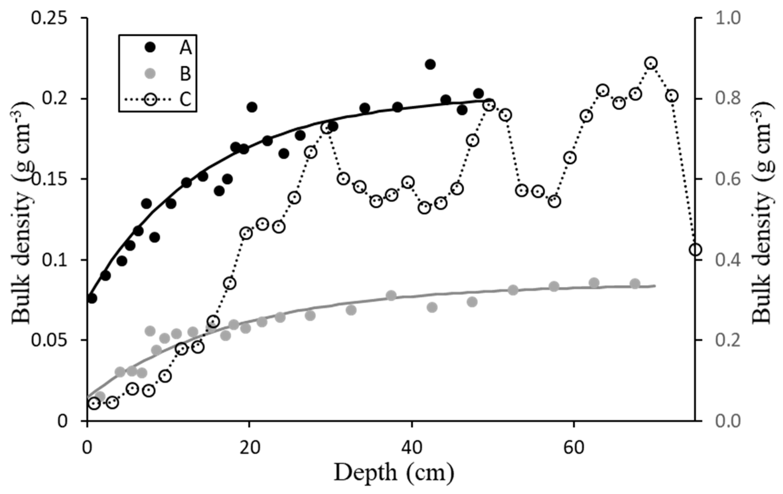
Figure 2.
The physical environment of the SWI region and the composite nature of the mass flows of solids and trace elements. Geometric figures entering the SWI represent different carriers that conform the composite flux of the tracer; among them, dots represent ions, in a dynamical exchange among the dissolved and solid-bound phases. Adapted from Abril and Barros (2022).
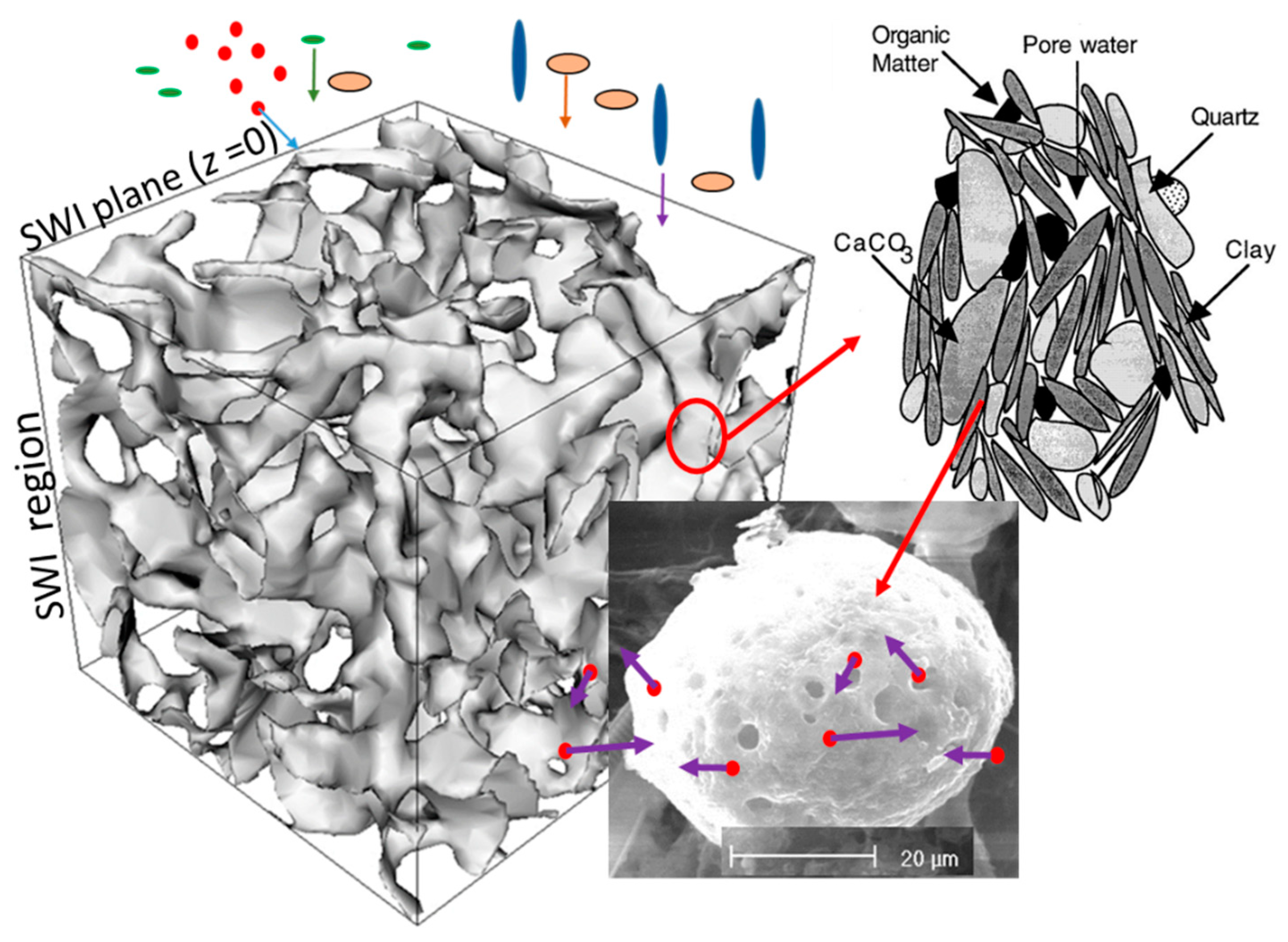
Figure 3.
Frequency distribution for initial 210Pbexc concentrations and SAR (w) (left panels) and statistical correlations (from bivariate correlated errors and intrinsic scatter) of 210Pbexc fluxes and initial concentrations with SARs (** in R2 means significant at 99% confidence level; N.S. is not statistically significant). The analysis uses normalised (to the arithmetic mean of each core) values from 11 varved sediment cores. Data from Abril and Brunskill (2014).
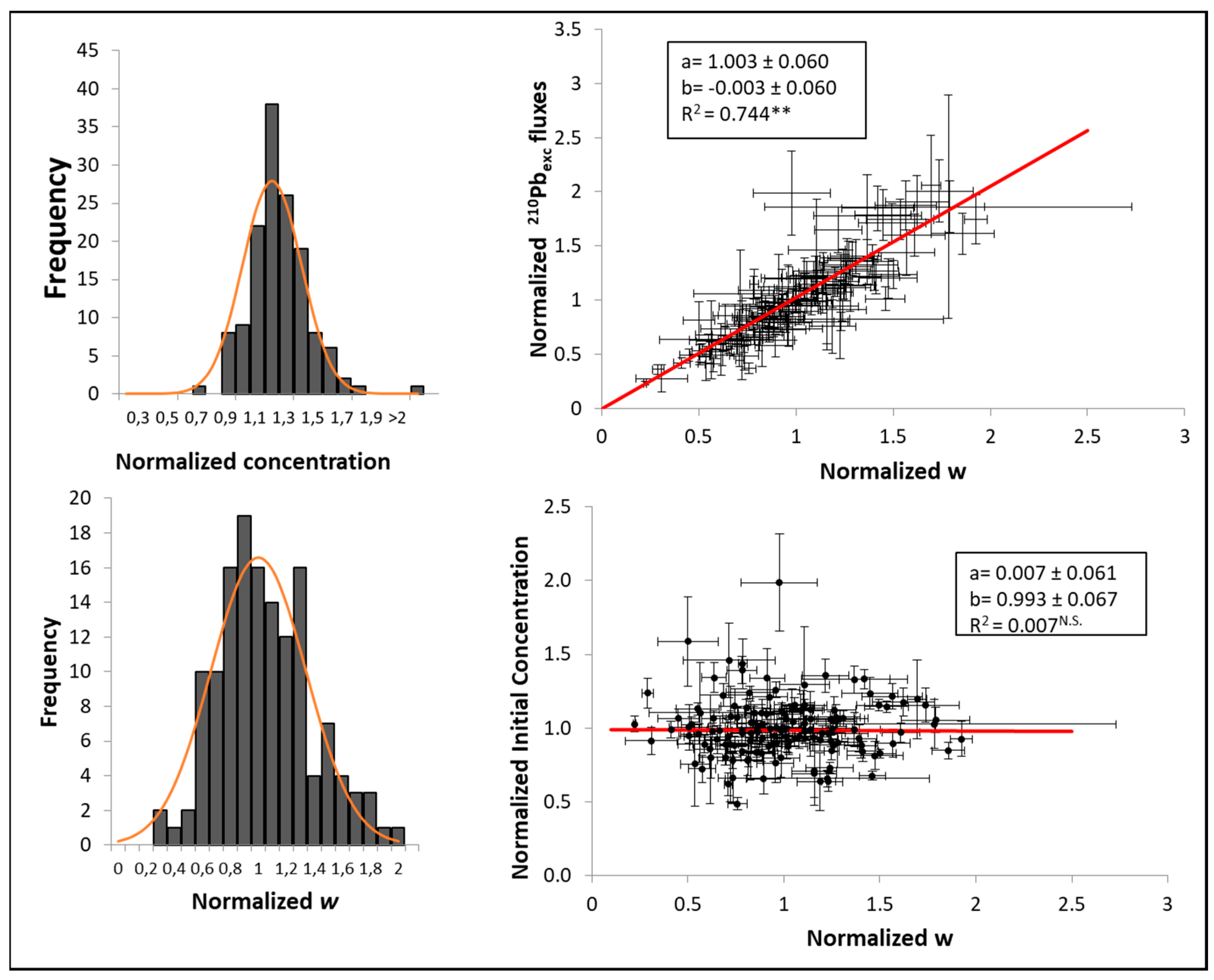
Figure 4.
210Pb-based dating models grouped by their involved assumptions on the functioning of the sedimentary system. Commonly used short names are indicated.
Figure 4.
210Pb-based dating models grouped by their involved assumptions on the functioning of the sedimentary system. Commonly used short names are indicated.
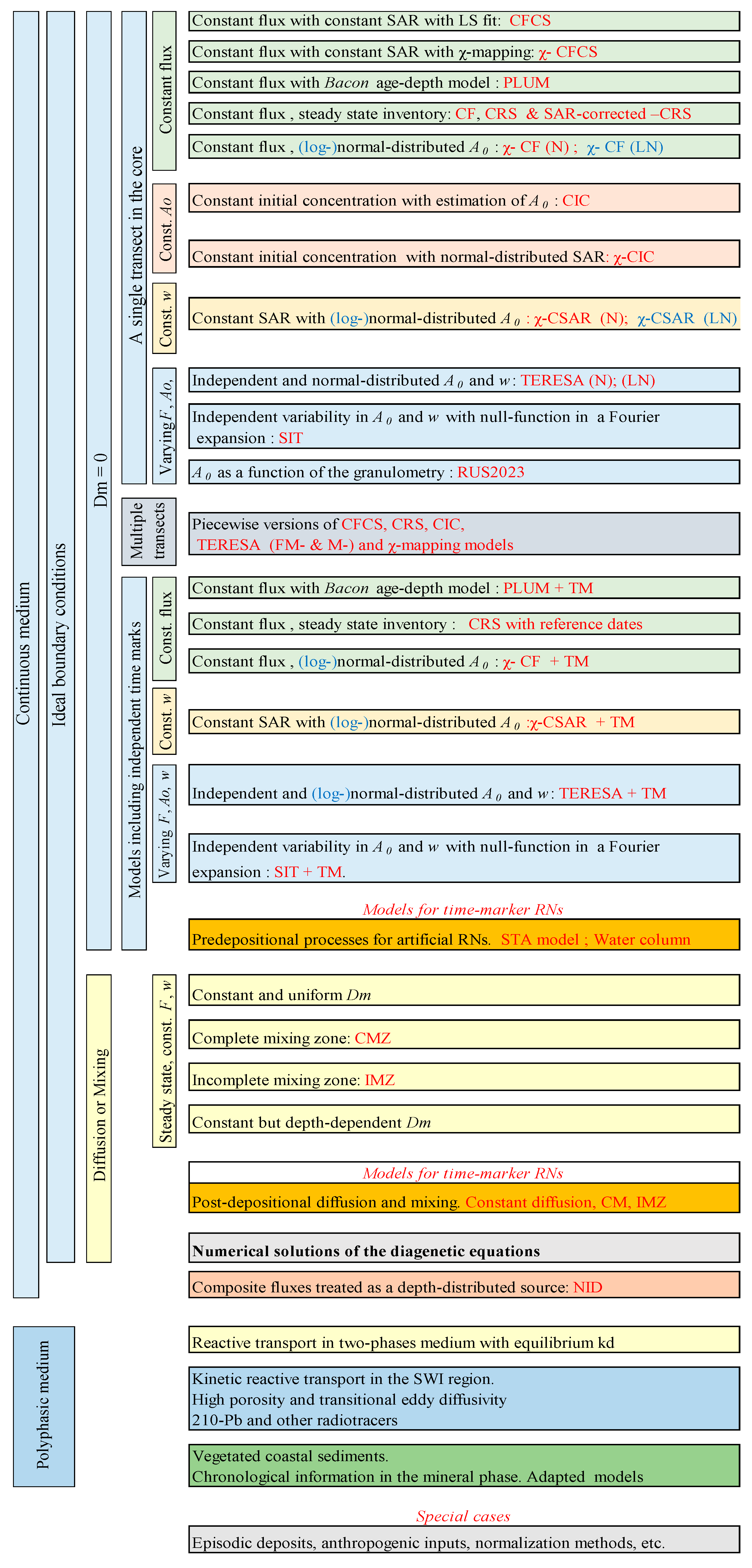
Figure 5.
Example of a cluster analysis. Ln[A(m)] plot for a varved sediment from Lake Zabinskie (data from Tylmann et al., 2016). Two jump discontinuities define three transects (r1, r2, and r3). The continuous lines are the linear fits from a piecewise CFCS model (see text). The records of palaeofluxes (plotted in the secondary y-axis) have been reconstructed from the empirical ( ) and the chronology from varves. Note that models that assume a constant flux within each transect are affected by model errors. Note in Transect 1 how a continuous trend of decrease in fluxes is not distinguished from an exponential decay in the fit r1. A study of this core with the piecewise version of several dating models can be seen in Abril (2019; 2020).
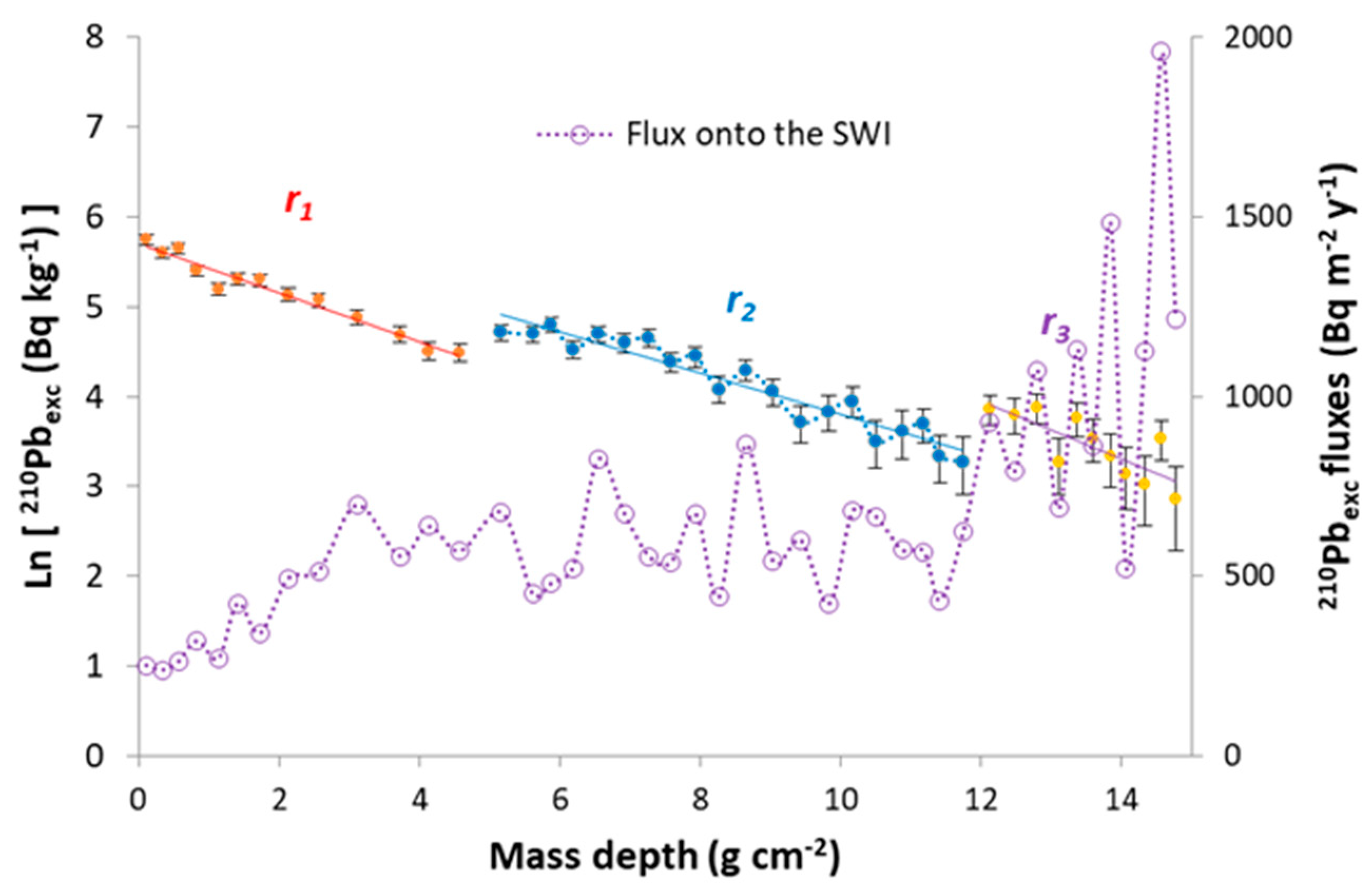
Figure 6.
Example of application of a set of models assuming constant flux to a varved sediment core from Kevojärvi Lake with a complex 210Pbexc profile (raw data from Haltia et al., 2021). The exponential fit (least squares) to Eq. 12 corresponds to the CFCS model. The χ-CF model closely fits the empirical data. The chronologies from varves, the above two models, and the CRS model are depicted on the secondary y-axis. Propagated errors are not depicted for the sake of clarity. See Abril (2023c) for a more detailed discussion.
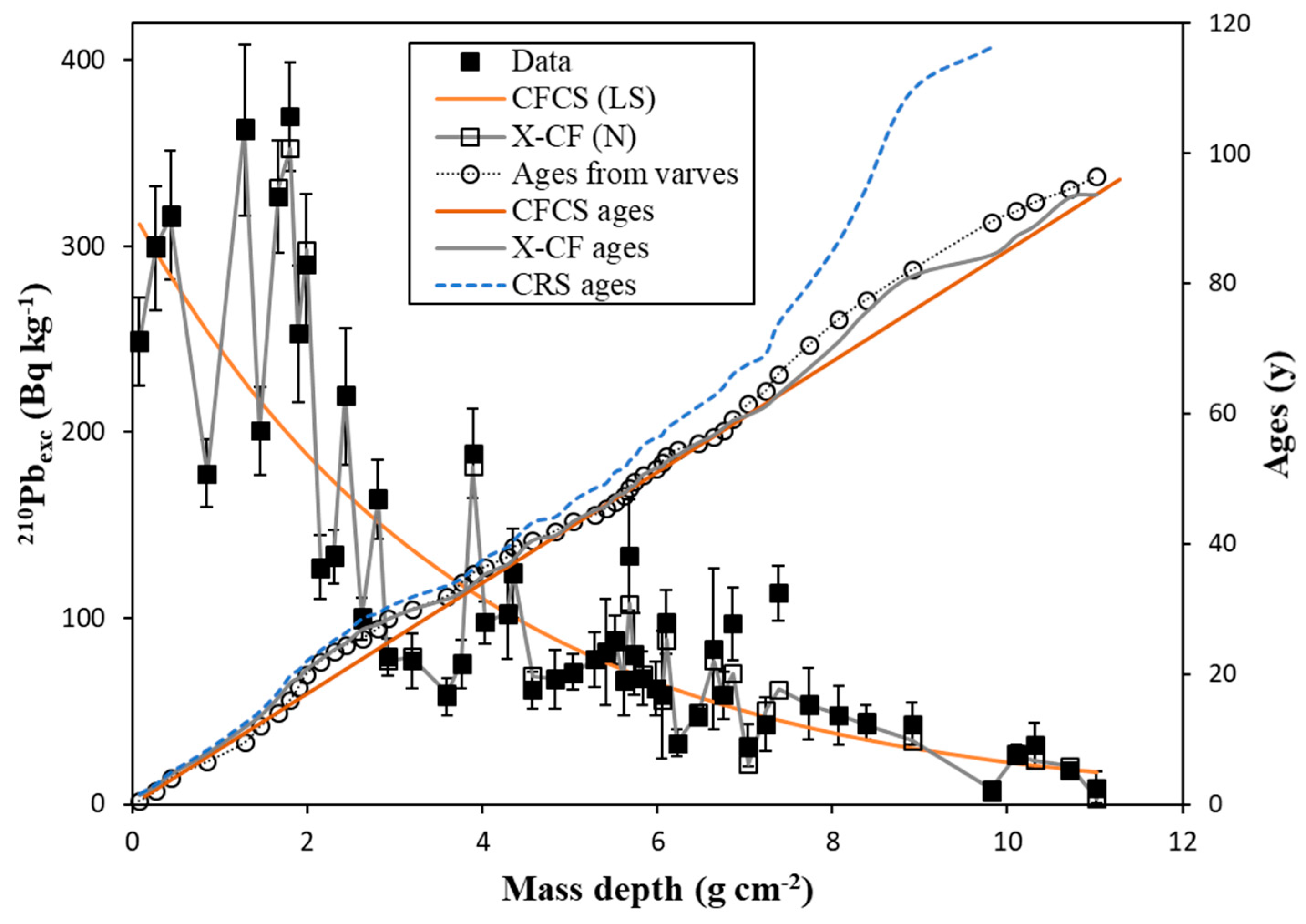
Figure 7.
Example of application of three χ-mapping models to the varved sediment core from Kevojärvi Lake: χ-CIC, CSAR and TERESA. Normal distributions have been used in the three cases. The corresponding chronologies are depicted on the secondary y-axis, along with the ages from the varves.
Figure 7.
Example of application of three χ-mapping models to the varved sediment core from Kevojärvi Lake: χ-CIC, CSAR and TERESA. Normal distributions have been used in the three cases. The corresponding chronologies are depicted on the secondary y-axis, along with the ages from the varves.
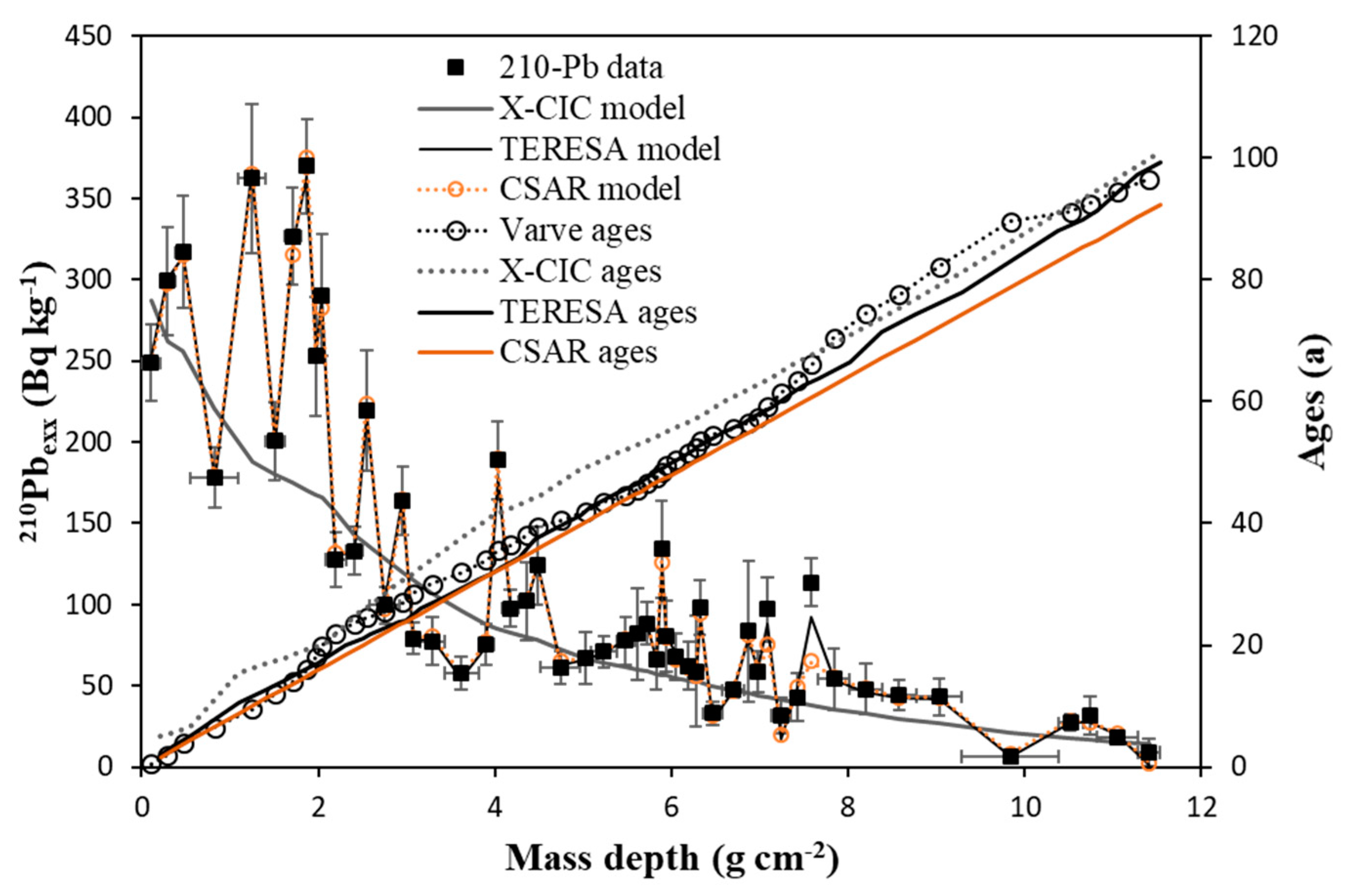
Figure 8.
Chronology produced by the χ-CF model using a time mark with the objective function of Eq. 15, for a varved sediment sampled in 2007 in Lake Lazduny, Poland (raw data from Tylmann et al., 2013 - their core LAZ 07/02). The time mark is one of the varve ages, and the figure plots the chronologies for 200 solvers around the minimum χ.
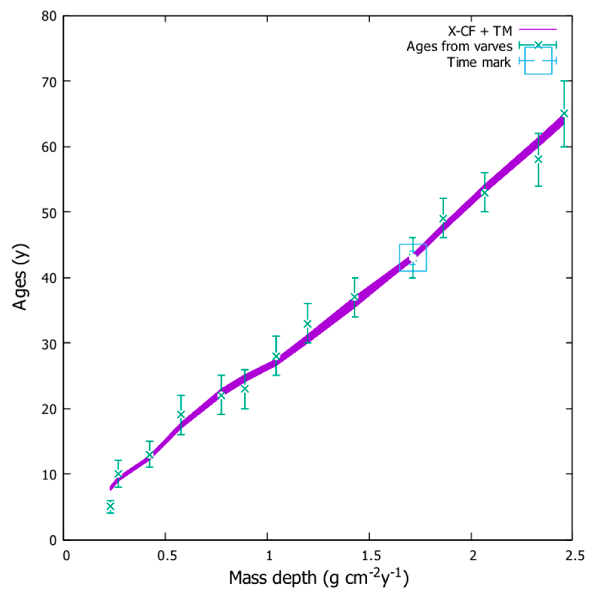
Figure 9.
210Pbexc versus mass depth profile for a varved sediment from Lake Zabinskie (raw data from Tylmann et al., 2016), along with the chronologies obtained from varves, a raw CRS model, and the piecewise CRS model when using one and two reference dates (1963 and 1986, from 137Cs data). Error bars are 1σ propagated uncertainties, and are reported only for one case, for the sake of clarity.
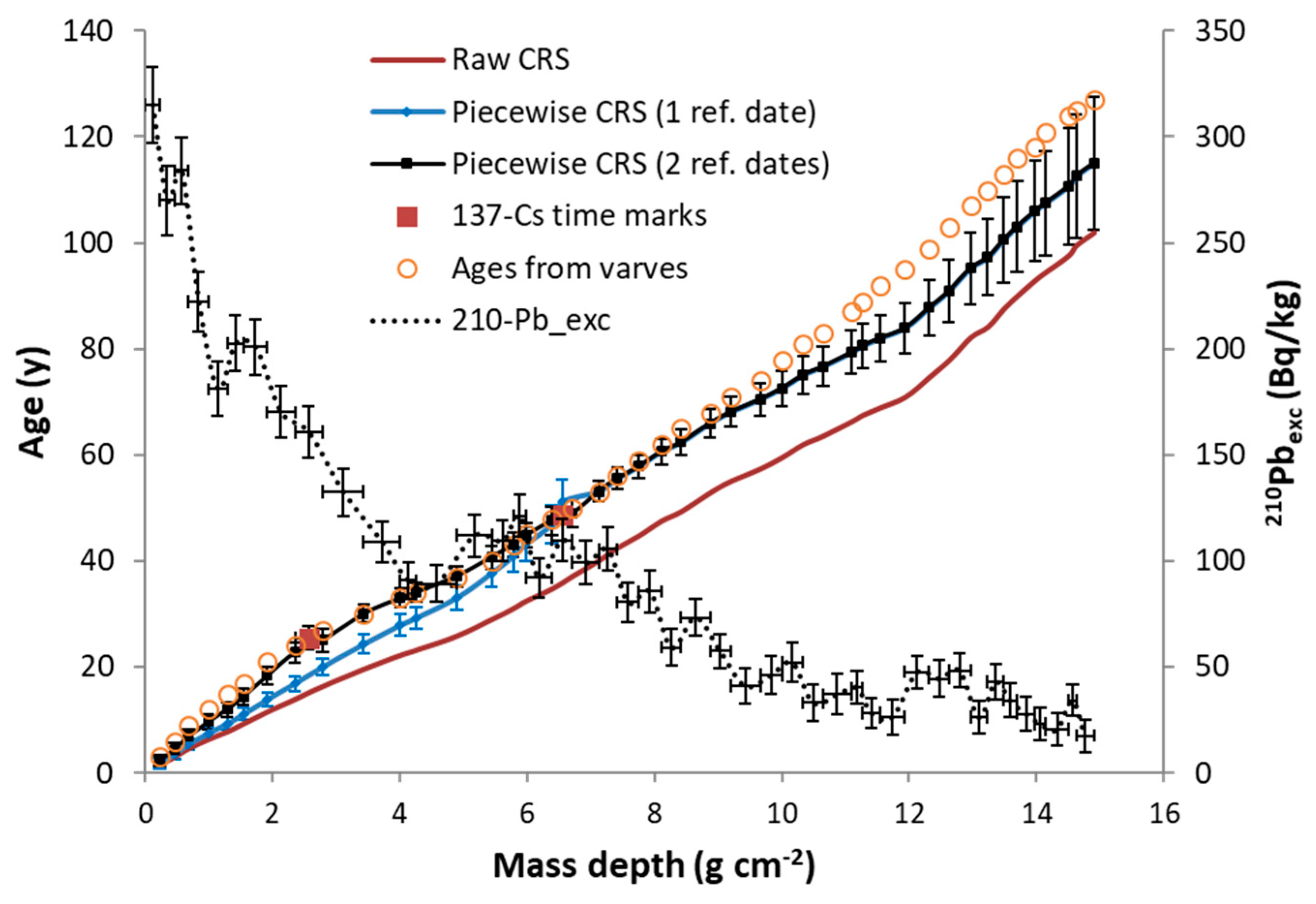
Figure 10.
Example of models considering diffusion applied to a sediment core sampled in the Gulf of Tehuantepec (raw data from Ruiz-Fernández et al., 2009). Model 1 uses
Figure 10.
Example of models considering diffusion applied to a sediment core sampled in the Gulf of Tehuantepec (raw data from Ruiz-Fernández et al., 2009). Model 1 uses
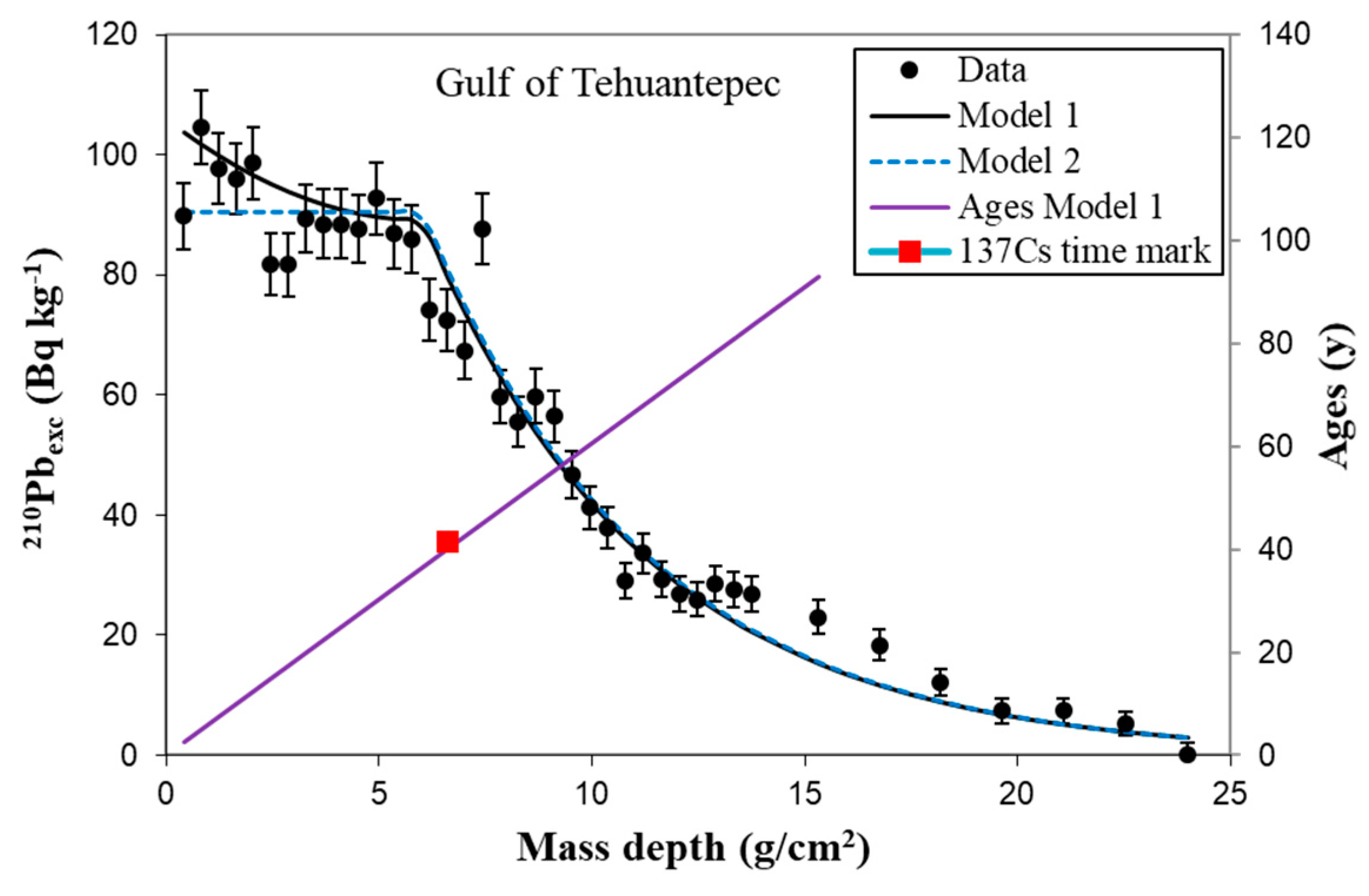
Figure 11.
210Pbexc mass activity concentrations versus mass depth profile with subsurface maximum. Sediment core 87A, sampled in 1987 in Skan Bay (Sugai et al., 1994). The continuous line is the best fit from a non-ideal deposition model with an exponential penetration pattern (adapted from Abril and Gharbi, 2012).
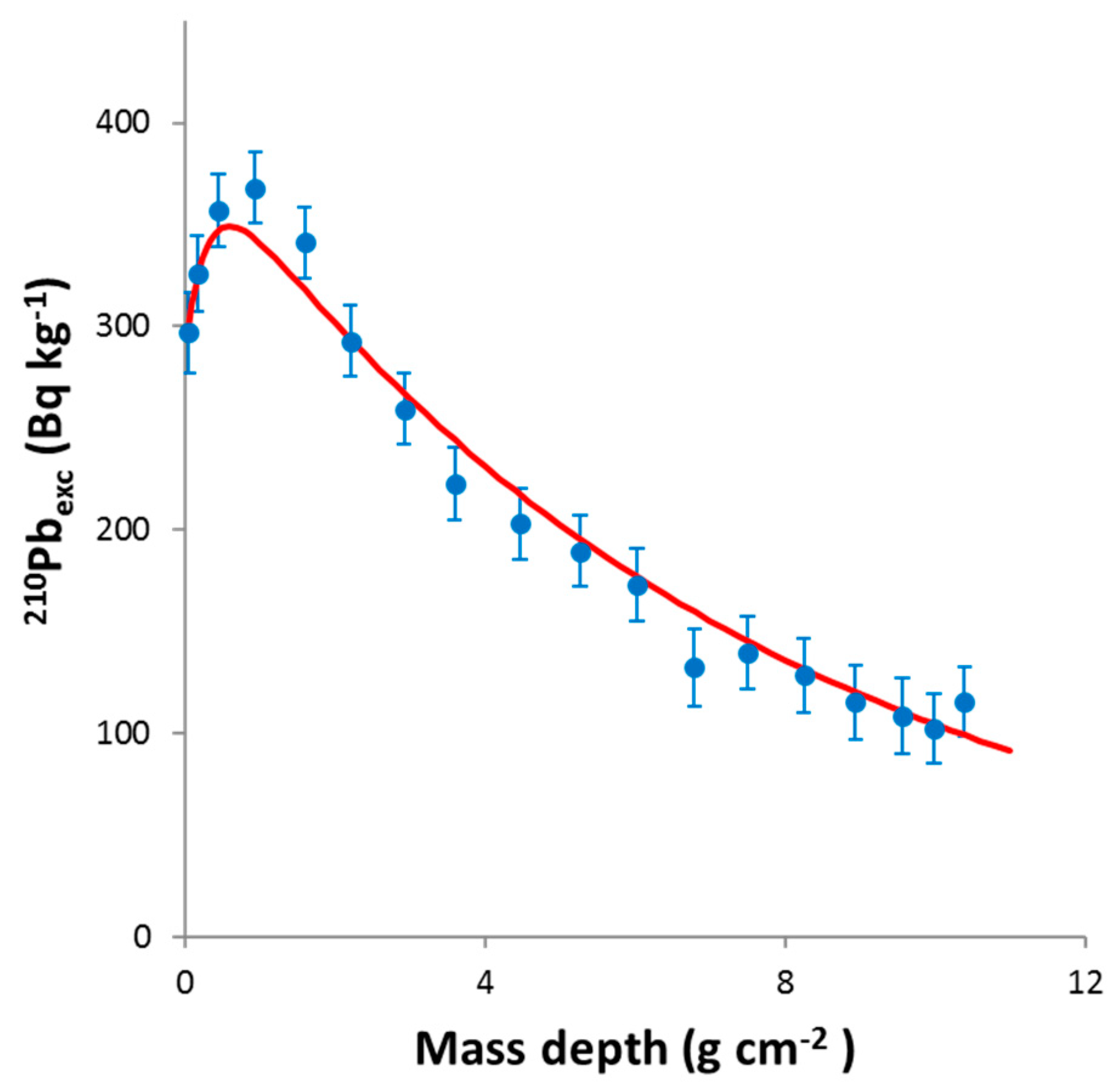
Figure 12.
Mass activity profiles for a tracer that mimics 134Cs. They are computed at different times with the numerical model for reactive kinetic transport by Abril and Barros (2022). Simulates the conditions for 134Cs from Chernobyl fallout in Lake Sniardwy, Poland, with a known history of concentrations in the water column. Model outputs are compared against empirical data for three cores sampled at site II in the lake at different elapsed times (data by Robbins and Jasinski, 1995). Horizontal bars define the depth intervals for the measured sediment slices (only depicted for the 1986 core).
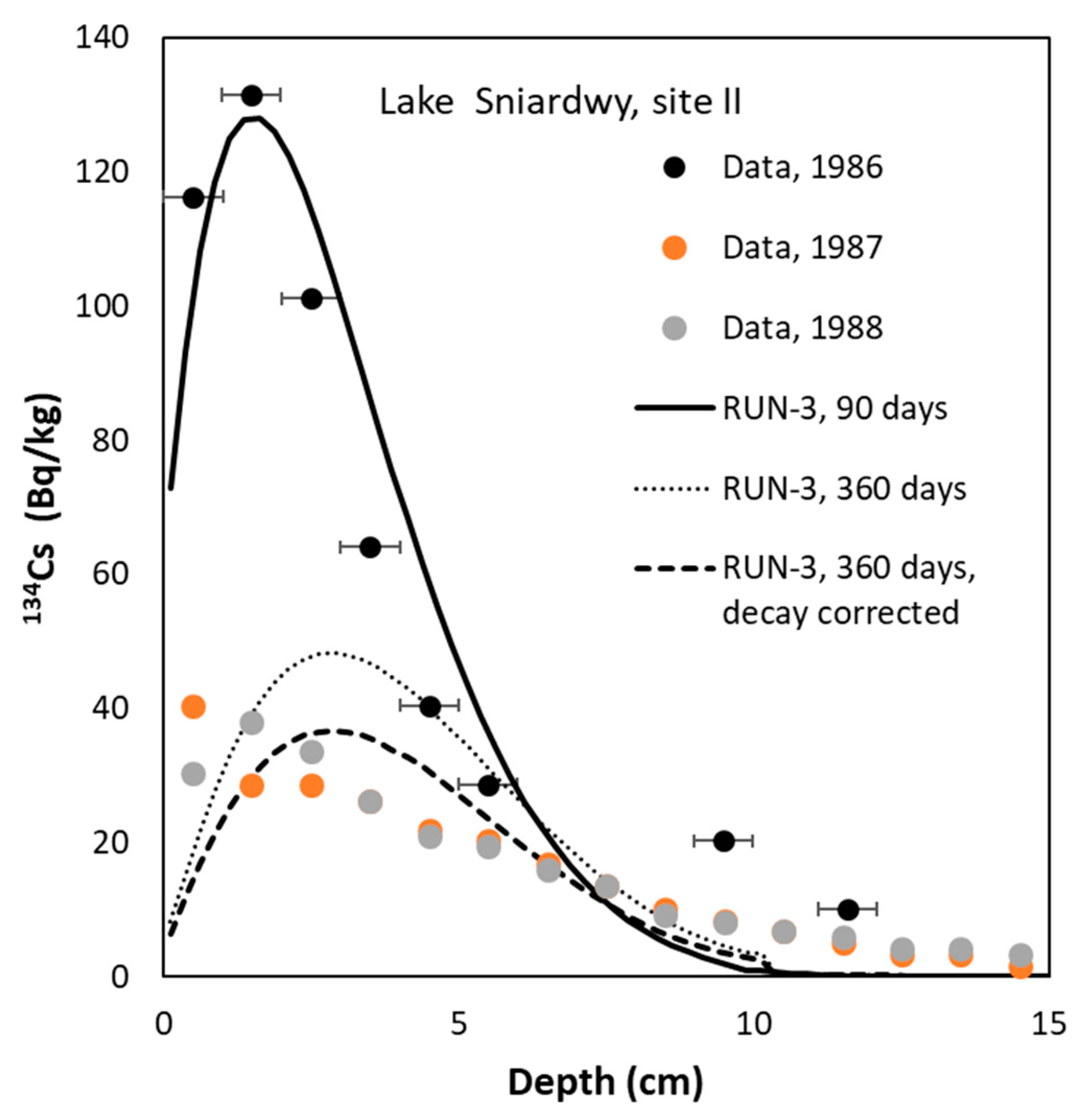
Disclaimer/Publisher’s Note: The statements, opinions and data contained in all publications are solely those of the individual author(s) and contributor(s) and not of MDPI and/or the editor(s). MDPI and/or the editor(s) disclaim responsibility for any injury to people or property resulting from any ideas, methods, instructions or products referred to in the content. |
© 2025 by the authors. Licensee MDPI, Basel, Switzerland. This article is an open access article distributed under the terms and conditions of the Creative Commons Attribution (CC BY) license (http://creativecommons.org/licenses/by/4.0/).
Copyright: This open access article is published under a Creative Commons CC BY 4.0 license, which permit the free download, distribution, and reuse, provided that the author and preprint are cited in any reuse.


