Submitted:
28 February 2025
Posted:
18 March 2025
You are already at the latest version
Abstract
We propose a novel extension to the recently developed non-commutative Riemannian foliated branch-cut quantum gravity (BCQG). On basis in an extended Faddeev–Jackiw symplectic deformation of the conventional Poisson algebra, we investigate non-commutativity effects on a symplectic topological manifold that provides a natural isomorphic setting composed by a triad of canonically conjugate scalar complex fields which comprise quantum complementary dualities. The resulting extended manifold spans the canonical BCQG cosmic scale factor and, in addition to its complementary quantum counterpart, outlined in the perfect fluid domain of Hermann Weyl, a scalar-complex inflaton-inspired field.
By constructing a triad of quantized fields underlying a noncommutative spacetime, this extension allows the elaboration of a scenario where the original branch-cut domain coexists with a complex scalar inflaton-type field, settled on a plateau of a strong gravity interaction structure. Alongside shaping this structure settled on a background composed by the primordial energy, radiation-, quintessence-, stiff-, baryon- and dark matter, combined with the spacetime components of the scalar Ricci curvature at different orders, cosmic inflation is driven. The presence of the inflaton field in the present formulation transcends the character of a simple reference field, to the extent that its original motivation has been to driven inflation, a role played by the original formulation of the BCQG.
The resulting symplectic algebraic extension allows additionally a liaison with primordial cosmic density perturbation predictions based on heuristic derivations of the scale invariance of the primordial spectrum of the Universe, as well as with eternal inflation and primordial chaotic cosmic mechanisms proposals.
Given the peculiar characteristic of BCQG in overcoming the primordial singularity, the non-commutative symplectic extension proposal, due to the complex character of the constituent fields, additionally outlines the evolutionary process of the mirror Universe that encompasses analytically continued complex conjugate
Friedmann's-type equations. This brings unique characteristics to the main scenario for the BCQG cosmic evolution, with a mirrored parallel evolutionary Universe, adjacent to ours, nested in the structure of space and time. The evolutionary process of the mirror Universe occurs in the negative sector of cosmological thermal time, and is characterized by a continuous cosmic contraction, with a systematic and continuous increase in temperature and a decrease in entropy before reaching the transition region to the current stage of the Universe. In contrast, the subsequent present evolutionary stage of cosmic expansion is characterized by a positive complex cosmological-time sector, accompanied by a systematic decrease in temperature and increase in entropy.
On basis on complementary analytically continued Friedmann’s-type equation, combined with a quantum approach based on the Ho\v{r}awa-Lifshitz quantum gravity, we describe the dynamic evolution of the Universe’s wave function, unfolding unprecedented predictions for the cosmic evolution and inflation.
This approach offers a new perspective to explain the accelerated cosmic expansion of the Universe, strongly suggesting that non-commutative algebra induces the late accelerated growth of the wave function of the Universe as well as of the corresponding scale factor and its complementary quantum counterparts. In contrast to the conventional inflationary model, where inflation requires a remarkably fine-tuned set of initial conditions in a patch of the Universe, non-commutative foliated quantum gravity, analytically continued to the complex plane, captures short and long scales of spacetime, leading to an evolutionary cosmic dynamic through a topological reconfiguration of the primordial cosmic matter and energy content. Still, we consider in this work the interplay between naturalness and a fine-tuning set constraining of the cosmological initial conditions. This result introduces new speculative framework elements regarding the reconfiguration of matter and energy due to an underlying non-commutative spatio-temporal structure as a driver of spacetime cosmic acceleration.
Keywords:
branch-cut cosmology
; Wheeler-DeWitt equation
; non-commutative quantum gravity
1. Introduction
The chronological evolution of the Universe comprises different phases, of which the recombination and decoupling periods stand out, as well as a ‘primordial’ era characterized by inflation, followed by the dominant phases of radiation, matter and, currently, a dark energy dominated period, which is widely assumed to be the main cause of the accelerated cosmic expansion.
In this work, we focus mainly on the inflationary period, proposing a novel extended approach to the recently developed non-commutative Riemannian foliated branch-cut quantum gravity (BCQG) [1].
We investigate the effects of imposing an extended enhanced non-commutative symplectic deformation of the conventional Poisson algebra on a topological manifold that conveys a natural isomorphic setting of a canonically conjugate triad of dual vector spaces. The extended triad approach encompasses the cosmic scale factor BCQG and two complementary dual quantum counterparts, outlined in the Hermann Weyl’s perfect fluid domain and the inflaton theory of exponential expansion of the early Universe [2]. This scenario allows the coexistence of the quantum domain of branch-cut gravity with an inflationary mechanism that, although controversial for assuming an entire Universe starting essentially from nothing, has had remarkable success in explaining relevant qualitative and quantitative properties of the Universe [2,3]. Among them, the approach to the origin of the large-scale structure of the cosmos stands out, based on quantum fluctuations in the microscopic inflationary region, amplified to cosmic size, becoming the seeds for the structure growth of the Universe.
Furthermore, based on this extended scenario, additional conceptual elements, such as density perturbations, grounded on heuristic derivation of the scale invariance of the primordial spectrum of the Universe, as well as predictions of an eternal inflation and even primordial chaotic mechanisms associated with the origin of the Universe, contribute to broadening the descriptive basis of the original BCQG formulation in order to incorporate elements of standard inflation conceptions.
Moreover, in view of the peculiar characteristics of BCQG in overcoming the primordial singularity, this formulation makes it possible, - due to the complex character of the non-commutative symplectic extended composition -, to make predictions about the evolutionary scenarios of the mirror Universe by means of complex- and complex-conjugated Friedmann-type BCQG equations materialized in a super-Hamiltonian that describes the wave function of an evolving Universe contemplating two unfolding phases, from negative to positive cosmological time. This brings unique features to the main BCQG scenario of cosmic evolution, with a parallel, mirror-like, evolutionary Universe adjacent to ours, nested in the fabric of space and time, with its evolutionary process in the negative sector of cosmological thermal time corresponding to a contraction process followed by a continuous expansion in its positive temporal sector. These characteristics open up a range of opportunities involving a reverse process to cosmic inflation in the mirror sector.
Returning to the aforementioned scenario, the assumed continuous contraction of the mirror Universe is accompanied by an increase in temperature and a decrease in entropy before reaching the cosmic transition region. In the subsequent domain to the transition region, the continuous expansion of the Universe is accompanied by a systematic decrease in temperature and an increase in entropy corresponding to the positive sector of the complex cosmological time. Using this formulation, we describe in the present investigation the dynamical evolution of the wave function of the Universe, and then, in another contribution, in the final stages of preparation [4], we describe the evolution of the cosmic scale factor and its complementary dual quantum counterparts, with unprecedented results.
2. A Review on BCQG
The proposed theoretical approach follows the branch-cut quantum gravity (BCQG) framework [1,5,6], based on the WheelerDeWitt [7] and the Hořava-Lifshitz [8] formulations, incorporating elements of symplectic geometry and non-commutative algebra [1] to investigate the interplay between small-scale quantum effects and large-scale cosmic evolution. BCQG provides moreover an alternative descriptive approach for cosmic evolution in comparison to conventional inflationary theories by building a quantum gravity environment through a fundamental restructuring of the conventional topological spacetime geometry rather than relying on specific initial conditions and ad hoc mechanisms.
Additionally, as previously stated [1], this approach offers a fresh perspective on the generation of relic gravitational waves and a possible solution to unresolved cosmological puzzles, such as the horizon and flatness problems. As previously mentioned [1], the realization of a non-commutative algebra structure induces the capture of short and long spatio-temporal scales, driving not only the evolutionary dynamics of the Universe’s wave function and the cosmic scale factor but also a reconfiguration of matter on small and intermediate scales, inducing the generation of relic gravitational waves, a topic to be addressed in a future investigation.
The symplectic non-commutative BCQG approach, as previously emphasized [1], was assembled by means of a deformation of the conventional Poisson algebra, and enhanced with a symplectic metric, based on the Faddeev-Jackiw two-fields quantization formulation [9,10] and extended in this contribution to a triad of dual and complementary quantum fields. Motivated by the compactification study of the properties of topological spaces, the non-commutative symplectic algebra is reflected in the validity of differential graded algebra with finite dimensional cohomology (compactification) and a rational Poincaré duality [11,12], which comprises harmonic foliations with minimal leaves on a Riemannian manifold [13], a crucial topic to embrace BCGQ. In other words, the Poisson brackets have the form , and because of the antisymmetry of the Poisson brackets, the automatically correspond to a symplectic block structured metric, no further assumptions required (for the details see [1]).
As previously stressed [1], BCQG comprises two foliation levels. The first level may be understood by assuming a D-dimensional Euclidean manifold associated to a given analytically continuation to the complex plane metric , carrying coordinates . Following canonical steps, a preferred time-direction may be set up by defining a time function and assign a specific time to each spacetime coordinate . Then we may decompose the manifold into spatial slices encompassing all points with the same ‘time-coordinate’. At this point, caution should be taken. This is because there is no time variable in the WDW equation in its original formulation, an intriguing feature for an equation with the ambition of describing the dynamics of quantum spacetime. Regardless of the long debates raised by the WDW equation about the nature of time, it is important to emphasize that in this conception should be highlighted as a non-dynamical parameter. The gradient of the time function can be used to define a vector normal to the spatial slices, with the lapse function ensuring normalization with respect to the metric, and the lapse defined in terms of the time coordinates and related to . In the projectable Hořava-Lifshitz gravity, N is restricted to a Euclidean time function only (see [14,15]). In our proposal, this restriction is overcome. In short, similarly to what occurs in general relativity based on the ADM-foliation tecnique [14], foliation in BCQG consists of slicing up the spacetime into three-dimensional spacelike hypersurfaces of constant time, relative to the global time function. For a coordinate (or stationary) observer at , his spatial coordinates remain constant after a time ‘lapse’ at . The second foliation level of BCQG is characterized by an analytically continued Riemannian foliation which corresponds to the reciprocal of a complex multi-valued function, the natural complex logarithm function , a helix-like superposition of cut-planes, which correlates Riemann sheets, with an upper edge cut in the n-th plane joined with a lower edge of cut in the (n + 1)-th plane. The BCQG Universe’s scale factor maps an infinite number of Riemann sheets onto horizontal strips, which represent in the branch-cut cosmology the evolution of the time-parameter dependence on horizon sizes. The patch sizes in turn map progressively the various branches of the function which are glued along the copies of each upper-half plane with their copies on the corresponding lower-half planes. In the branch-cut cosmology, the cosmic singularity is replaced by a family of Riemann sheets in which the scale factor shrinks to a finite critical size, - the range of , associated to the cuts in the branches, shaped by the function —, well above the Planck length. In the contraction phase, as the patch size decreases with a linear dependence on , light travels through geodesics on each Riemann sheet, circumventing continuously the branch-cut, and although the horizon size scales with , the length of the path to be traveled by light compensates for the scaling difference between the patch and horizon sizes. Here, represents the dimensionless thermodynamical connection between the energy density E and the pressure P of a perfect fluid thus enabling the fully description of the equation of state (EoS) of the system. Under these conditions, causality between the horizon size and the patch size may be achieved through the accumulation of branches in the transition region between the present state of the Universe and the past events. Conventionally, the theory deals exclusively with finite-dimensional real symplectic spaces. The BCQG in turn extends the ontological domain of general relativity to the complex plane. In BCQG, the presence of a branch-cut and a branch point defines the domain of the scale factor of the analytically continuous Universe for the complex sector, overcoming the presence of a cosmic singularity. The BCQG offers additionally a theoretical alternative to inflation models [2,3], based on the mathematical augmentation technique and notions of closure and existential completeness [16], which have proved highly useful in both quantum mechanics [17,18,19] and pseudo-complex general relativity (pc-GR) [20], with direct physical and cosmological manifestations. For the sake of completeness, we present in the following foundational elements of the BCQG formalism [1,5,6].
The complete line element of the BCQG quantum gravity, resulting from the complexification of the FLRW metric [21,22,23,24], in line with the ADM-foliation [14], may be expressed as [25,26,27]
In this expression, denotes analytical continuation to the complex plane, where r and t represent real and complex space-time parameters, respectively, and k denotes the spatial curvature of the multiverse, corresponding to negative curvature (), flat (), or positively curved spatial hypersurfaces (). represents the foliated scale factor, and denotes the lapse function. The gauge invariance of the action in general relativity yields a Hamiltonian constraint that requires a gauge-fixing condition on the lapse function (see [28]). We extend the gauge fixing constraints further to the algebraic structure of the BCQG action.
At this point it is important to emphasize that BCQG does not require any external mechanism for its realization, nor even the assumption of a Universe created from nothing. BCQG is based on a peculiar kind of topological quantization. In simplified terms, topology involves the study of the preserved properties of a geometric object under continuous deformations, such as stretching, twisting, crumpling and bending. In this sense, the topology and geometry of spacetime play a fundamental role in our understanding of quantum gravity. In general, a topological quantum field theory comprises topological invariants, properties that are insensitive to changes in the shape of spacetime, where the correlation or partition functions of the system, — computed by the path integral of metric-independent action functionals —, stand out. A relevant aspect of quantum gravity approaches, a topic of intense debate, is their subdivision into two large classes, depending on whether they are spacetime background-dependent or background-independent. Spacetime in general relativity, unlike the Newtonian and special relativity Minkowski approaches, is not fixed but it is dynamical, in the sense that its shape depends on its matter and energy content, which implies no privileged spacetime background [29].
Background independence and covariance, concepts intertwined with the diffeomorphism invariance of gravity, elevated to the status of a fundamental principle, represent basic building blocks of general relativity [30] and in the quantization of gravity [31]. As highlighted by Lee Smolin [31], general relativity was conceived as a principle theory instead of a constructive theory. Similarly, BCQG follows the same logical conception developed by Albert Einstein, that is, instead of following the fundamentals of a constructive theory, based on the description of particular phenomena, fields or particles that constitute nature, specified in terms of dynamical equations of motion that the constituents obey, BCQG in turn, was conceived as a principle theory, guided this way by universal principles. Although this statement should imply future advanced studies, BCQG should obey in consequence the same fundamental principles as general relativity. More precisely, BCQG should fit into the context of a background-independent covariant theory that obeys diffeomorphism invariance. Following the logical principles of a principled theory, the concept of quantum topology would therefore apply to BCQG with respect to the presence of topological invariants, properties that are insensitive to changes in the shape of spacetime, a topic that requires further study. In this context, future studies should focus on identifying candidates for topological invariants of BCQG, among which the torsion tensor stands out as the most relevant. This is because results presented in this contribution indicate that spacetime torsions would represent essential ingredients to drive the acceleration of the Universe as well as the generation of relic gravitational waves.
As pointed out [32], Einstein’s gedenken elevator experiment broughted to the Equivalence Principle that asserts the local equivalence of inertial and gravitational effects, leading him to associate the gravitational field with the space-time metric. And since the gravitational field is a dynamical object, the metric must therefore also be dynamic, that is, should also depend on the composition of matter and energy in the Universe. At this point, conventional topological quantization finds, in BCQG, a peculiar aspect. The evolution of the scale factor in the convencional cosmology is governed by the Friedmann equations which depends on the the total energy density and pressure of the universe. In this sense, the scale factor characterizes the global properties of the Universe, representing a crucial element in determining the overall size and shape of the metric configuration of the universe. Assuming the FLRW metric, in order do not violate the cosmological principle, preserving the homogeneity and isotropicity of the Universe, in conventional cosmology, the dimensionless scale factor is a real scalar quantity and has only a temporal dependence.
In BCQG in turn, the function corresponds to a helix-like superposition of cut-planes, the Riemann sheets, with an upper edge cut in the n-th plane joined with a lower edge of cut in the (n + 1)-th plane. maps an infinite number of Riemann sheets onto horizontal strips, which represent in the branch-cut cosmology the time evolution of the time-dependent horizon sizes. The patch sizes in turn maps progressively the various branches of the function which are glued along the copies of each upper-half plane with their copies on the corresponding lower-half planes. In the branch-cut cosmology, the cosmic singularity is replaced by a family of Riemann sheets in which the scale factor shrinks to a finite critical size, — the range of , associated to the cuts in the branch cut, shaped by the function —, well above the Planck length.
In a formulation based on the multiverse concept [33] and the analytic continuation technique in complex analysis applied to the FLRW metric [21,22,23,24], Friedmann-type equations for a complexified version of the CDM model () yield (see [25,26,27]):
In these expressions, represents the BCQG cosmological constant. These equations due to the nature of BCQG allow the construction of a set of complex conjugate Friedmann’s-type equations. These complex and complex-conjugate Friedmann-type equations materialize in a super-Hamiltonian developed below.
3. Commutative BCQG
The starting point of this study is the commutative BCQG action which depends on the branching scalar curvature of the Universe, , and on its covariant derivatives, , in different orders [1,5,6], and whose development was based on the formulation of Hořava-Lifshitz [8]:
In this expression, represent running coupling constants, denotes the Planck mass, and by imposing a maximum symmetric surface foliation [1], the branching Ricci components of the three dimensional metrics are given as:
where the variable change , with , was introduced. Moreover, the trace of the extrinsic curvature tensor , represented by [1,5,6,34], is given as:
Exploring the ADM-type formalism domain, for the metric given by equation (1), adopting the gauge, the three-metric corresponds to a projectable analytically continued quantum gravity formulation:
Applying standard canonical quantization procedures to the BCQG action, the canonical momentum reads
and the resulting Hamiltonian density
becomes
In this expression, the running coupling constants depict the matter-energy contributions of radiation (), baryon matter (), curvature (), quintessence (), cosmological constant dark energy (, and stiff matter () (for the details see [35,36] and references therein).
3.1. Commutative BCQG: Two-Fields Approach
In what follows, we adopt, as a formal approach strategy, to initially address the formulation developed in previous contribution [1]. In this proposal, an extended dual field commutative manifold was introduced, composed by a mini-surperspace of variables (), composed by a quantum counterpart-reference to the BCQG scale factor the perfect fluid conception of Hermann Weyl [37] denoted by , characterized by a dimensionless quantity , whose canonically conjugated momentum is defined as . The corresponding Hamiltonian contribution is given as:
The variables and span quantum reference variable spaces. After simplifying the notation and combining (10) and (11), the following super-Hamiltonian density results:
The fields u and v obey the following commutative Poisson algebra
3.2. Commutative BCQG: Three-Fields Extension
In order to make contact with an inflaton-inspired proposal, we consider, in what follows, a commutative mini-surperspace triad of variables (). In this proposal, represents a hypothetical scalar inflaton-type field, analytically continued to the complex plane, which was originally conjectured, in the real domain, by Alan Guth [2,3], to drive cosmic inflation in the very early Universe. According to Guth [2,3], the main property of the physical laws that makes inflation possible is the existence of states with negative pressure, whose effects produce a repulsive form of gravity identified in the standard Friedmann equations. Based on the Robertson-Walker metric, these effects are based on an energy-momentum tensor as a function of a scalar field , the inflaton, which leads to energy and pressure densities of the Universe expressed in terms of a potential, , which describes, in its original version, chaotic inflation. In the present work we also consider a simulation involving non-chaotic inflation.
We adopt for the action of the scalar field the following expression [38,39]
where denotes the inflation potential, defined in terms of the inflaton-type field and where represents a coupling function. In the following, by inserting into the BCQG action (11) the scalar field contribution (14), by applying conventional quantum field theory techniques, the corresponding contribution associated to the field is given as
the Hamiltonian associated with the extended mini-super-space of variables may be obtained. The resulting commutative Hamiltonian density then becomes
In what follows, we model chaotic inflation by adopting the potential [2] (see Figure (Figure 1))
and for the non-chaotic inflation, the Fubini potential [40] (see Figure (Figure 1))
In the following, we build a non-commutative three fields approach.
4. Extended BCQG Symplectic Non-Commutative Algebra
In order to extend the BCQG symplectic non-commutative algebra, we embrace a similar analytical strategy adopted in the elaboration of the non-commutative two-fields BCQG. We base our strategy firstly on the construction of an extended three-field commutative BCQG manifold, composed of an extended mini-super-space of variables (). Then, this extended commutative manifold is related to a non-commutative structure, based on an extended Faddeev-Jackiw symplectic-type phase space transformation applied to the mini-super-space of variables . The insertion of the field in the non-commutative symplectic formulation substantiates this way the extension of the BCQG scope in order to make contact with standard inflation approaches.
4.1. BCQG as a Gauge Theory
From a conceptual point of view, it is important to emphasize that BCQG formulation essentially constitutes a quantum gauge field theory. Characterized by a group of transformations of the field variables, known as gauge transformations, a quantum gauge theory postulates the Lagrangian and the dynamics of a quantum system are invariant under local transformations, in accordance with Lie algebra which encompasses fields and group generators. This condition, called gauge invariance principle, embraces the theory with a set of symmetries that fundamentally govern its dynamical equations.
Among the theoretical approaches commonly adopted to systematically identify symmetries and conserved quantities in a field theory, the Dirac formalism [41] and the Faddeev–Jackiw method [9,10] stand out. In order to accomplish conventional and elementary quantization of a dynamical system, the Dirac method for a given Lagrangian demands (i) to eliminate velocities in favor of momenta by adopting a Legendre transform that determines the corresponding Hamiltonian, (ii) to postulate canonical brackets among coordinates and momenta and finally (iii) determine the dynamics by imposing commutation rules encompassing the Hamiltonian. However, this procedure may fail when dealing with any singular Lagrangian and constrained dynamics [42]. The alternative approach of Faddeev–Jackiw [9,10], based on Darboux’s theorem, provides a symplectic and straightforward effective instrument to deal with gauge constrained systems and makes it possible to obtain the desired results — formulas for brackets and for the Hamiltonian — while avoiding canonical restrictions of the Dirac procedure.
In what follows, we will adopt an unorthodox perspective by proposing, as previously carried out [1], a reverse transformation from a set of noncommutative coordinates to commutative variables based on the Faddeev-Jackiw symplectic approach [9,10], extended to the triad , and assumed as dual an complementary quantum fields. In summary, following a procedure adopted previously [1], we adopt a reverse logic of the conventional Faddeev-Jackiw formalism, presupposing a character change for the variables , and , assuming as stressed before that they obey the non-commutative algebraic structure described by a non-zero Poisson bracket formalism.
We assume the extended domain of commutating () and non-commuting () coordinates are represented in general as
The commuting (on the left) and non-commuting (on the right) coordinates satisfy the following Poisson-brackets
the bracket on the left satisfies the commutative metric while the bracket on the right satisfies the symplectic metric, according to the following symmetry properties:
For practical purposes it is often advantageous to work in coordinates and to represent the elements of the symplectic algebra by matrices, where the standard symplectic matrix J, expressed in terms of the identity matrix I, obey the conditions , and .
The algebraic matrix structure of the commuting brackets on the left may be cast as
Using the left expression of equation (20), the algebraic matrix-structure above leads to the following non-zero commutative Poisson-brackets:
Symplectic geometry, in turn, whose origins date back to the Hamiltonian formulation of classical mechanics, is a branch of differential geometry and differential topology that studies symplectic manifolds, or more specifically, differentiable manifolds equipped with a closed non-degenerate 2-form. Using the symmetry properties synthesized in the expression on the right of equation (21), the matrix representation of a symplectic algebra may be cast as
For the non-commuting Poisson brackets, using equation (20), we obtain
In order to perform the three-field extension within the framework of non-commutative Riemannian foliated branch-cut quantum gravity (BCQG), based on an improved deformation of the conventional Poisson algebra, we connect the commutative algebraic structure with its non-commutative counterpart, by means of a symplectic topological manifold linear transformation:
Following the steps outlined on equations (A1), (A2), and (A3), we arrive at the non-commutative symplectic Poisson-type brackets synthesized in equation (A4). Applying the standard gauge fixing condition which states that the structure of the original equations remains invariant under coordinate transformations, so as to produce a result that is physically meaningful, we adopt in what follows the following settings for determining the matrix elements :
- (i)
- (ii)
- The resulting transformation expressions (26) should keep the original functional structure of the super-Hamiltonian, as a kind of ‘canonical structural gauge’, maintaining preserved the identities of the components composition, — coordinate power series disassociated from conjugate momenta contributions —, in short, avoiding mixing original algebraic elements through the adopted symplectic transformations, preserving the physical content logic related to the Hamiltonian formulation.
- (iii)
- First-order canonical momentum transformations are not subject to such constraint, since first-order linear momentum dependent terms do not alter the structure of the original Hamilton equations. This is because for transformations which contains linear momentum algebraic components combined with power series involving the fields u, v, and , the components of these power series contributions are `naturally’ incorporated into the different dynamical potentials, preserving the formal structure of the corresponding Hamilton’s equation.
- (iv)
- According to [12], symplectic reduction is at the heart of many symplectic arguments. In line with the Marsden-Weinstein-Meyer Theorem, which underpins the statement that whenever there is a symmetry group of dimension k acting on a mechanical system, the number of degrees of freedom for the position and momenta of the particles can be reduced by , symplectic reduction provides extremely symmetric symplectic manifolds. Moreover, from the previous two-field non-commutative algebra approach [1] we learn, assuming a kind of `symplectic gauge-reduction’ proposal, that the symmetries of a Hamiltonian dynamical system enables the reduction of the number of degrees of freedom of a given system, generating a lower ordering dimensional symplectic manifold, which in order to be so representative as possible, it demands to settle a symmetric and equalized representation; this corresponds to an additional demand, strictly followed in the adopted formulation, as we will see below.
An algebraic transformations that obeys all the previous condition does not change the non-commutative nature of the symplectic general algebraic structure, and obeys the fundamental gauge principle which states that the Lagrangian, and therefore the dynamics of the system itself, do not change under local transformations according to smooth families of operations of the Lie group. Applying all these conditions we arrive at the following restrictions for the components:
These conditions reduce the original symplectic matrix to the following form:
The topological-algebraic constraints previously approached result in the following transformed coordinates:
and
An important aspect to be highlighted is that, although the placed impositions imply significant formal simplifications, the most distinguishing attributes of the non-commutative nature of the original equations remain consistently incorporated. Still, the merits regarding the rigor of the analytical foundations applied in the present formulation, with respect to the implications of the non-commutative structure as inducing the acceleration of the Universe, remain pertinent.
4.2. The Role of Time in BCQG
When tracing the genesis of the problem of time in quantum mechanics, Jan Hilgevoord based his observations on the work of six of the founding fathers of modern quantum theory: Dirac, Heisenberg, Bohr, Schrödinger, von Neumann and Pauli, covering the period from 1925 to 1933, finding some coherence issues between the views of these authors. In this study, a mixture of notions from classical, quantum mechanics and the theory of relativity were found [43]. Although this topic is not the focus of the present work, it serves as an example that the problem of time in quantum mechanics, as well as in general relativity and quantum gravity is not new. And apparently we are far from finding a final definition to this issue. In this subsection we address some aspects involving the problem of time in QCG in order to contribute to its elucidation.
Time in quantum theory corresponds to an external element that, in a certain way, acts as a controller of all movement, identified either as an absolute quantity (similarly to Newtonian physics) or in the form of proper times characterized by a classical space-time metric, applicable to local quantum systems along their world lines. In other words, the reading of time corresponds to a classical clock underlying the quantum world. (For an useful discussion see [43,44]).
The dynamics of quantum systems in turn consists of individually undetermined stochastic ’quantum jumps’ between ’stationary’ states, or more properly, energy eigenstates [46], although time corresponds to a dynamic variable external to quantum systems flowing continuously. In this sense, the flow of time in non-relativistic quantum mechanics acquires an universal and absolute character, similarly to Newtonian mechanics.
In quantum relativistic theory, proper times assume the role of absolute time for local systems, i.e., systems that follow, albeit approximately, the world lines in spacetime. However, since quantum states are generically non-local, auxiliary time coordinates corresponding to arbitrary foliations of spacetime can then be introduced to define the dynamics of global states. This aspect of relativistic quantum mechanics is similar to the role of the t parameter adopted in BCQG.
In quantum gravity, time as an absolute quantity has no meaning. Therefore, by obeying the Wheeler-DeWitt equation, known as the timeless equation, the wave function of the universe corresponds to a functional in a configuration space consisting of spatial geometries and matter field configurations. In this ambiance, all dynamics is encoded in the matter field configuration entanglement underlying the universal configuration space, the `DeWitt-superspace’ [44].
Therefore, the evolutionary process referred to in quantum gravity in general, as well as in BCQG, does not allude to an `absolute’ time as a dynamic variable, but to the evolution of the different configurations of matter fields. It is precisely for this reason that the evolutionary equations of the wave function of the universe refer to derivatives in terms of the fields , , and , and not to temporal derivatives. Furthermore, the presence of the variables t in the mentioned equations refers in BCQG to parametric quantities related to spacetime foliations, making it possible to associate the term `evolution’ with a process connected to the systematically unfolding transformations of matter field configurations on the different Riemannian sheets.
4.3. Probability Interpretation of the Wave Function of the Universe
According to J.B. Hartle and S.W. Hawking [44], the quantum state of a spatially closed Universe can be described by a wave-function, , which is a functional on the geometries of compact three-manifolds , that depends on a metric and on the matter fields on these manifolds, . The wave-function of the Universe obeys the Wheeler-DeWitt second-order functional differential equation and is described not in a temporal sense, but instead in terms of the matter fields on these manifolds (see also [43,45,46,47]). In a similar sense, for Hawking and Page [48], the wave-function of the Universe, given as , is proportional to the probability of finding a 3-surface with metric and matter field configuration :
where corresponds to a volume element. The replacement of the time evolution of the wave function of the Universe by the (dynamical) evolution of the matter field configuration and, therefore, the absence of time in the conventional sense in the framework of quantum gravity is a characteristic of the classical Hamilton-Jacobi formulation of general relativity. In this context, the wave function corresponds only to a function of the “3-geometry”, that is, to the equivalence class of metrics subordinate to a diffeomorphism, more precisely, to an isomorphism of differentiable manifolds. In what follows, based on both Rovelli’s and Hawking’s interpretations, we adopt the term `probability density’ to establish a connection involving the BCQ and conventional quantum mechanics.
5. The Wave Function of the Universe in the Non-Commutative Three-Fields Formalism
As a result of the previously adopted gauge-transformations, from equation (11) we arrive at the following super-Hamiltonian:
In this expression, for notation simplicity, we eliminate the tilde identification of the commutative variables. By adopting the reverse mapping path proposal, the above equation materializes the effects of reconfiguration of the original super-Hamiltonian through the imposition of a non-commutative algebra. The resulting equation, although dependent on the original commutative variables, highlights this reconfiguration through the imposition of a structural composition that inserts new dynamic components into the original formalism, modulated by the parameters , , , . Unlike a conventional symplectic transformation, this procedure makes it possible to identify, in a comprehensible way, the striking outcome of the non-commutative algebraic transformations when compared to a standard formulation.
From expression (33), making the quadratic terms explicit, we obtain
Combining similar terms, from this expression we obtain
Assuming the perfect fluid radiation condition for the early Universe matter content, and naturalness condition, the corresponding expressions for the coefficients are shown in Table 1.
Canonical quantization procedures applied to the Hamiltonian (35) results in the the wave equation
where denotes the wave-function of the Universe. In this equation, the variables , , and along with their corresponding conjugate momenta , , and acquire the status of quantum linear operators which act on the wave-function of the universe:
Following the steps outlined in Appendix B, equation (36) is reduced to the canonical form (for the details see [49]):
Exploiting a relevant feature of the adopted canonical transformation (see Appendix B), which can be summarized in the freedom of choice of canonical variables, we opt for the following associations, , and . Evidently, the connections imposed by the relations (A7), (A8), (A9) and (A10) attribute to each variable , and a new identity when compared with their original counterparts, , and , forming a triplet of canonical complementary dual-conjugate quantum fields. Complementarity in conventional quantum mechanics is commonly interpreted in terms of duality and opposition, considering conjugate fields as dual and opposite. The formulation of quantum mechanics is shaped by complex, dual, and complementary Hilbert spaces. Quantum complementarity unifies duality and opposition in a consistent way, thus underpinning the physical world. This character of dual Hilbert spaces extends to quantum fields, when they experience sets of transformations in a non-commutative algebra, attributing to them new identities that materialize in the sharing of identities in comparison to fields originally belonging to a commutative algebraic structure. The concept of entanglement, coined in quantum mechanics to designate attributes of correlation related to conjugate variables, establishes that the quantum state of each field of a given group cannot be described independently of the state of the others, even when the particles are separated by large distances. In our view, we identify these aspects of quantum entanglement with the attributes of the present correlation, which fundamentally characterizes a non-commutative symplectic transformation of coordinates.
In the reverse Faddeev-Jackiw formalism proposed, the variables , , and are non-commutative, and after the symplectic transformation, the new canonical variables , , and , — and despite conforming a commutative set of variables —, they obey a set of non-commutatively structured equations, shaped by the corresponding parametric attributes of the Poisson-type non-commutative algebra. In summary, the resulting set of variables, , , and are canonically conjugate dual and complementary variables, which span reciprocal spaces, so the following relation between these variables holds:
and
The ideal fluid condition for the radiation era, assuming the parameter is a real quantity, , less a constant allows the variables separation of equation (38) in the form
with , and
The parameters ans may be assumed as real or imaginary quantities. In the first case, equations (41) and () may be cast as
In the second case, assuming and , equations (41) and () become:
5.1. Foliated Branch-Cutting Approaches to Classical and Quantum Gravity
Before performing calculations and interpreting the results, it is important to make a distinction between the classical approach of the branch-cut foliate formulation and its quantum counterpart. The classical formulation was based on S. Hawking and T. Hertog’s multiverse proposal [33] of a hypothetical set of multiple Universes existing in parallel and on the analytic continuation technique in complex analysis applied to the Friedmann-Lemaître-Robertson-Walker (FLRW) metric [21,22,23,24]. As a result of this approach, a closed system of Friedmann-type field equations that sweeps a hypothetical maximally symmetric and homogeneous set of superposed multiple Universes, with a cosmic scale factor analytically continued into the complex plane, was obtained. Complexification of the FLRW metric resulted in a linearly independent superposition of these field equations associated with infinitely many poles, in line with Hawking’s multiverse composition of an infinite number of simultaneously occurring primordial Universes arranged along a line in the complex plane with infinitesimal residues. The introduction of a regularization variable allows shifting the limits of the Friedmann-type field equations beyond the primordial singularity. Imposing in turn that the multiple singularities of the field equations are confined to the same Universe and using a Riemann integration, a branch-cut solution was obtained. The regularization function allows the contour solution-lines to move around the branch cut, since the integration limits can be shifted without altering the continuity of the resulting functions so long as the contour-lines does not cross the complex branch-point related to the branch-cut. The introduction of a regularization function at this stage of the formulation is not equivalent to changing the limits of the integration of Friedmann’s equations to avoid the presence of singularities, since essential or real singularities cannot be removed simply by any coordinate transformation. The technical procedure adopted admit to circumvent the singularities, — that would otherwise be inescapable —, which in turn become branch points. To accomplish this proposal, the assumption of continuity at the local level prevails, i.e., there is some neighborhood of the branch-point, say , close enough although not equal to , to characterize a small region around local patches where is single-valued and continuous. The cuts in the branch cut are shaped in turn by the function which, besides the range, characterizes also the foliation regularization of and domain extension. This procedure moreover allows a formal treatment consistent with the Planck scales that establishes, according to the multiverse concept, the region of confluence between quantum mechanics and general relativity. The descriptive emphasis of the evolutionary process of the foliated quantum Universe is focused on the imaginary sector associated with the scale factor . This is because each Riemann sheet of the multiple leaves associated with comprises a new Universe, thus composing an infinity of Universes connected by a branch-cut. In the real sector, however, the different multiverses behave as disconnected, linearly independent in their evolutionary process. In this context, although the evolutionary perspective of branch-cut cosmology contemplates the imaginary sector of the Universe’s scale factor, the formal consistency of the proposal is also supported by the real sector.
Concerning the quantum approach of the branch-cut foliate formulation, we adopt as stressed before a topological quantization method applied to the BCQG scale factor. Topological quantization can be applied to any field configuration whose geometric structure allows the existence of a principal fiber bundle, — a locally product space, although it may have a different topology globally. In the case of gravitational systems with an infinite number of degrees of freedom, a theorem proves the existence and uniqueness of such a bundle. According to the theorem, any solution of the minimally coupled Einstein equations to any gauge matter field can be represented geometrically as a principal fiber bundle with spacetime as the base space. The structure group, isomorphic to the standard fiber, follows from the invariance of the metric of the base space with respect to Lorentz and gauge transformations. The topological invariants of the corresponding principal fiber bundle lead to a discretization of the parameters entering the metric of the base space [50]. The quantization of the BCQG Lagrangian density is achieved by raising the dynamical variable and the conjugate momentum to the category of quantum operators. Although the association between the classical variable and the quantum version are underlying present in this process of topological quantization, the formulation of BCQG provides a new analytical conception. In this conception, the overcoming of the primordial singularity by means of a Riemannian structure that allows it to be bypassed is replaced by a quantum leap. In other words, the primordial singularity that is replaced in the branch-cut formalism by a branch point is present in the form of an infinite succession of individual singularities, continuously interconnected, overcome however by means of quantum leaps of the solutions.
As highlighted in a previous article [1], regarding the presence of a mirror Universe, the BCQG resembles cyclic and bouncing models that experience infinitely alternating periods of rapid expansion and contraction, surpassing the primordial singularity, without an end and without a beginning. However, when we examine from an ontological and epistemological point of view the BCQG and compare its theoretical construction with the other formulations, the similarities between the two lines of investigation are quite remote. Cyclic bouncing models, for example, are proposed based on an analytical investigation of the evolution of the Universe and implemented mainly in an ad hoc way, through parameterizations, cosmic wedge diagrams and other aesthetic foundations. The foliated analytical continuation of quantum gravity, in turn, from an ontological and epistemological point of view, — except for the complexification of the standard metric, combined with the concepts of multiverse —, contemplates theoretical foundations and theoretical investigation procedures similar to those of general relativity. BCQG shares with general relativity the same fundamental questions, the same objects of investigation, the same claims about the nature of being and existence, that is, the same first principles of its conceptual philosophy. In this sense, the realization of a transition that overcomes the primordial singularity giving rise to a mirror Universe is not the result of an ad hoc proposition, but the natural result of an evolutionary process of fundamental equations of the general relativity type, generated through ontological, methodological and epistemological theoretical procedures based on field theory. Likewise, the realization of the transition region that overcomes the primordial singularity does not require the imposition of an artificial mechanism to guarantee its existence, being the natural result of a topological restructuring of space-time.
5.2. Naturalness
In the study of the evolution of the Universe, we are faced with an epistemic limitation regarding the scientific realism, — the under-determination of any scientific theory by evidence, a problem that particularly affects the frontiers of quantum gravity. Therefore, in order to overcome these limitations, it becomes essential to establish an organizing and guiding principle in order to make non-empirical models viable, enabling the realization of consistent and precise calculations, avoiding in particular the assumption of adjustment parameters. Proposed by Weinberg [54], the principle of naturalness serves as a standard method for classifying and organizing the distinct theoretical terms of highly intricate field theoretical approaches, as well as providing guidance for understanding the various interaction couplings associated with the dynamic composition of matter, energy and even primordial sources of gravitational waves. This principle suggests that the underlying parameters in quantum field theory are all of the same ‘size’, in appropriate units or, more precisely, that a given quantum field theory can only describe nature at energies below a certain cutoff scale [54]. In this context, we adhere to the principles of naturalness, normalizing the coupling constants to unity.
As an additional message, it is important to remember the meaning of the term ‘fine-tuning’, when applied to the evolutive Universe. In this case, the term “fine-tuning” is used to characterize sensitive dependences of the facts or properties of the Universe on the values of certain parameters. Subject to fine-tuning, the description of the evolving Universe depends sensitively on parameters that describe the form, arrangement, composition and material properties of its constituents. Fine-tuning in particular is a requirement of standard inflation model concerning finely tuned initial conditions in order to explain the degree of flatness and homogeneity observed in the Universe. In this sense, the criterion of naturalness represents a kind of no fine-tuning condition in a rather different sense, which applies to theories in quantum field theory and plays a large role in contemporary particle physics and cosmology.
5.3. Boundary Conditions
In the following we determine solutions for equations (41), (), and (). The boundary conditions of the solutions are based on the Bekenstein criterion [55], which provides an upper limit for the Universe’s entropy, following the proposition presented in [1,5,6]. Accordingly, a key factor to understand the upper bound of entropy contained within a certain finite region of space with a finite amount of energy is the Bekenstein bound, a fundamental criterion which settles the basis for the generalization of entropy and the second law of thermodynamics for non-gravitational systems. Applied to the primordial Universe by considering the connected spatial region within the particle horizon of a given observer, i.e., the locus of the most distant points that can be observed at a specific time in an event, an upper bound, given by , for the entropy S and energy E of a system enclosed in a spherical region of radius R, was conjunctured:
with denoting the upper entropy limit of the Bekenstein bound. The implications of the Bekenstein criterion are striking since it establishes initial physical conditions that impact the evolution, symmetries and conservation laws of elementary particles in the early Universe. The fulfillment of the criterion would imply a non-singular, isotropic and homogeneous primordial Universe with entropy, temperature, and baryon number equal to zero.
The total entropy of a black hole, according to the Bekenstein criterion, is proportional to the number of Planck areas needed to cover the event horizon, where each area corresponds to one unit of entropy. In the non-commutative branched gravitation, we assume that the primordial singularity is equally covered by a certain number of Planck areas, whose numerical value in turn corresponds to the total primordial entropy of the Universe (see also [44,56]. We also assume that the dimensions of this boundary region correspond to the most distant observable points, while respecting causality. To comply with this requirement, we consider an appropriate cosmic distance, denoted as , between a pair of objects at any instant of time t, and the corresponding distance at a reference time . We then establish this relation as . This means that the relation between the two distances is modulated by the scale factor of the BCQG Universe. This implies that for we have . Regarding the wave-function of the Universe, adopting a conventional probabilistic point of view, this condition implies, at , , assuming a normalized wave-function. Thus, the following boundary conditions can be considered: on the mirror Universe, and and on the present Universe, and .
5.4. Solutions for , , and
In order not to overextend this contribution, we present below a small group of figures representing some of the solutions to the equations developed. The examples presented represent extracts of the descriptive conceptual potential of BCQG with regard to the description of the evolutionary Universe.
5.4.1. Solutions
By mean of the successive approximation method, we found the following algebraic solution for equation (45)
with the conditions and , , as , and and and as . For equation (47), obtain the following solution through the successive approximation method:
with similar conditions as the previous ones for the parameters , , , and .
Figure 2 shows on the left an Argand-type diagram which refers to the transversal structure of the distribution of real and imaginary family sample solutions of the wave equation (45) for the wave-function , depicting its geometric properties. The figures on the right show plots of sample individual solutions corresponding to the conditions on the top, and , below. For the figures, the naturalness cosmological initial condition was assumed and . The Argand diagram indicates an overlapping winding between the real and imaginary components of the multi-valued function , reflecting the intense correlation between matter and energy encapsulated in the potential . Inserting a complex polar representation of , a complete description of this wave-function is portrayed by copies, or branch-cut Riemann sheets, in the complete complex cut-plane extending from , forming a Riemann surface. The behavior of the solutions indicates that the complex function is meromorphic, — that is holomorphic and therefore analytic on the upper and below cut planes. Similarly, Figure 3 shows on the left an Argand-type diagram solution of the wave equation (45) and on the right plots of sample individual solutions corresponding to the conditions on the top, and , below, assuming a fine-tuning set of the cosmological initial contidions. Figure 4 show sample solutions of the wave equation (47) for the wave-function , assuming the naturalness condition, and , with on the left images of the figure and on the right images of the figure. The result on the left of Figure 4 resembles the predictions of the big bounce theory, which is based on the notion that the evolution of the Universe corresponds to a cyclical and non-linear natural phenomenon that sustains a deceleration stage of the expansion process conforming a contraction phase. The results of the images on the right of Figure 4 show an expanding and cyclical Universe, with the amplitudes of the wave-function growing systematically intensely in contrast to increasingly shorter Planck time intervals. This behavior characterizes a Universe in accelerated expansion as a result of the reconfiguration of primordial matter and energy and the capture of small- and large-scales of spacetime due to the non-commutative symplectic algebraic structure. Figure (Figure 5) show sample family solutions of equation (47) for the wave-function assuming the naturalness condition. The upper-left and lower-left figures correspond respectively to the boundary conditions and while the upper-right and lower-right figures correspond respectively to the boundary conditions and . According to BCQG, the transition between the mirror Universe, in a contracting phase, and its current expanding counterpart occurs through a quantum leap, exemplified in the Figure (Figure 5), corresponding to the upper-right and lower-right images and boundary conditions and .
5.4.2. Solutions
The algebraic solution for the differential equation () is
Figure 6 exhibit sample family solutions of the wave equation () for the wave-function , assuming the naturalness condition. The figure on the left shows an Argand-type transversal structure mapping the distribution of real and imaginary numerical sample solutions of the wave-function . The figure on the right show plots of the solution of equation () given in (52). The blue lines correspond to real parts of the solutions while the orange lines to imaginary components. The behavior of the solutions corresponding to the wave function , as a function of , a support field that is both dual and complementary to the scale factor , once again highlights a singular aspect of BCQG, the emanation of a mirror Universe, nested within ours in the space-time domain of negative cosmological time, offering a consistent alternative to the original proposal of the inflation model of a Universe arising from nothing as a result of vacuum fluctuations. Due to the nature of the wave equation of the dual field , the Argand-type diagram reveals that the imaginary part of the solutions is restricted to the negative sector of the real part, while the opposite occurs for the real part. A crucial aspect of the solutions, highlighted in the image on the right of the Figure (Figure 6) is their continuity, indicating a hypothetical connection between the current Universe and its mirror counterpart BCQG.
5.4.3. Solutions
The algebraic solution for the differential equation (), in case of chaotic inflation, is
The results for the wave-function corresponding to Figures (Figure 4) and (Figure 5), on the right present unique and consistent characteristics and similarities. The evolutionary behavior for both solutions, indicates a cyclical and rapidly expanding Universe, with the amplitudes of both wave functions, and , systematically increasing in contrast to the systematic reduction of the corresponding Planck time intervals, a compelling indication of cosmic acceleration in the inflationary period. To our knowledge, this is the first time that solutions of a wave equation of an inflaton field are known, in the context of quantum gravity, evidencing related and complementary behavior of the inflaton field and the cosmic scale factor. These results further indicate that the conventional inflation model, although introduced historically in an ad hoc manner, includes crucial elements that characterize the cosmic acceleration drive. This behaviour indicates a growing disruptive evolution increase in the branched-gravitation expansion phase, prior to the BCQG transition region characterized by the overcoming of the primordial singularity, as predicted in the standard model, and prior the wave-contraction phase. Furthermore, as we will see later, when we consider the dynamical equations involving the cosmic scale factor, the presence of the inflaton field in the present formulation of BCQG adheres consistently to the reconfiguration of spacetime as a result of a noncommutative symplectic algebraic structure, contributing in a unique manner for cosmic acceleration. The branched transition region may be outlined according to three different perspectives: (i) a classical view of a kind of ‘transition topological portal’, (ii) a quantum view region which contemplates a topological quantum leap, and (iii) a mixed conception in which both previous conceptions consistently intersect, shaped on basis of the Bekenstein criterion (see [1]). The topologically foliated branch-cut quantum structural representation of the transition region involving the contraction and expansion phases resembles a topological spacetime shortcut, as a kind of foliated wormhole structure. Theoretical implications of the existence of topological shortcuts in spacetime imply a challenge to our understanding of fundamental physical principles, such as causality or still open topics such as the origin of primordial cosmological material seeds. Accordingly, the standard inflation model conception of the creation of the present Universe from nothing, as a result of virtual vacuum fluctuations, falls apart when we examine the results of Figure 5 and Figure 6. These results indicate that the present Universe might have its origin in an earlier phase through a possible distant spacetime shortcut. We may conjecture if this tiny correction would be, in principle, detectable by homodyne-type measurements, — a method of extracting information encoded as modulation of the phase and/or frequency of an oscillating signal, a gravitational wave for instance. Additionally, we may even conjecture if this tiny correction would be detectable after long propagation lengths for a wide range of throat radii and distances to the shortcut, even if the detection takes place very far away from the throat, where the spacetime is very close to a flat geometry. Figure 7 show sample family solutions of the wave equation () for the wave-function , assuming the naturalness condition. The figure on the left corresponds to chaotic inflation while the figure on the right to non-chaotic inflation.
6. Final Remarks and Conclusion
Quantum field theory in non-commutative spacetime leads to an uncertainty relation for coordinates analogous to the Heisenberg uncertainty principle, whose lower bound has given rise to the minimum scale problem. An unique feature of non-commutative field theory is the realization of a mixing between ultraviolet and infrared radiation (UV/IR), which characterizes an interrelation between short and long-range scales, absent in commutative quantum field theories (see for instance [11]). The theoretical problems above were also identified by Seiberg–Witten [57]. On basis of the weak gravity conjecture, the notion of hierarchical UV/IR mixing was implemented with scalar fields by Lüst and Palti [58]. In addition, the deep-low IR and far-high UV connection, according to Craig and Koren, by studying IR dynamics from UV divergences, in the context of UV/IR mixing, could even solve (part of) the hierarchical naturalness problem [59].
Different hypotheses can be raised to explain the cosmic inflation acceleration. A compelling possibility emulates from the electroweak hierarchy problem, based on an inspiring article [60]. The authors, in their study of perturbative dynamics of a particular set of non-commutative field theories, found an intriguing mixing of the ultraviolet (UV) and the infrared (IR) domains, identified with the observation that high energy UV virtual particles in loops produce non-analyticity at low momentum, interpreted as IR divergences. This finding, a realization of the mixing between the the short-range, high-energy ultraviolet (UV) and long-range, low-energy infrared (IR) phenomena, according to the authors, arises from the underlying non-commutativity, a phenomenon reminiscent of the channel duality of the double twist diagram in open string theory (for the details, see [60]). (For an alternative discussion see [61]).
In short, in the field theory prevails the conception that the origin of the IR/UR mixture results from the capture of large and small scales by the presence of a non-commutative structure. Translating this conception to quantum gravity, the non-commutative symplectic quantum structure of spacetime, through the capture of small-, medium- and large-scales, generates, on the one hand, a topological restructuring of space-time and, on the other, a restructuring of the primordial distribution of matter and energy.
Finally, the presence of the inflaton-type field , similarly to the complementary quantum counterpart field of the the canonical BCQG cosmic scale factor enables the materialization of a spatial plenum, a transition space between the present Universe and its mirror counterpart completely filled with matter, instead of a spatial vacuum or a topological quantum transition region, providing a theoretically consistent medium required by seed conceptions.
In particular, the presence of these fields could provide the physics environment which allows, quantitatively, to determine how density fluctuations in the early Universe are imprinted in anisotropic signals indicating the presence of material seeds. In particular, the presence of these fields could provide imprints of gravitational waves generated before the recombination process and about the phase transition involving the early Universe and its mirror counterpart. Generated long before the recombination phase, the anisotropic distribution of these gravitational waves could reveal the effects of density perturbations seeded by the inflation process, providing new clues for a better understanding of the primordial density perturbations of our early Universe and thus improving our understanding of the inflation theory.
Author Contributions
Conceptualization, C.A.Z.V.; methodology, C.A.Z.V. and P.O.H. and R.R. and B.A.L.B. and J.A.deF.P. and D.H. and F.W. and M.N-M.; software, C.A.Z.V. and B.A.L.B. and M.R. and M.N-M. and R.F.S. and J.G.G.G; validation, C.A.Z.V. and P.O.H. and R.R. and B.A.L.B. and D.H. and J.A.deF.P. and F.W.; formal analysis, C.A.Z.V. and R.R. and P.O.H. and J.A.deF.P. and D.H. and F.W. and B.A.L.B.; investigation, C.A.Z.V. and P.O.H. and J.A.deF.P. and M.R. and M.N-M. and F.W. and B.A.L.B.; resources, C.A.Z.V.; data curation, C.A.Z.V. and B.A.L.B.; writing—original draft preparation, C.A.Z.V.; writing—review and editing, C.A.Z.V. and B.A.L.B. and P.O.H. and J.A.deF.P. and D.H. and M.R. and M.M. and F.W. and R.R.; visualization, C.A.Z.V. and B.A.L.B.; supervision, C.A.Z.V.; project administration, C.A.Z.V.; funding acquisition (no funding acquisition). All authors have read and agreed to the published version of the manuscript.
Acknowledgments
P.O.H. acknowledges financial support from PAPIIT-DGAPA (IN116824). F.W. is supported by the U.S. National Science Foundation under Grant PHY-2012152.
Appendix A A Three-Field Faddeev–Jackiw Symplectic Algebra Extension
Adopting as a simplification the condition , , and , since this setting does not change the structure of the approach, maintaining the same polynomial orderings of the corresponding variables, - and as a consequence the same structure of the matter and energy potential in the BCQG action, we can reduce the matrix M to the expression
On basis on the sets (23) and (25), we consider first the Poisson brackets that involve only one-coordinate and one-momentum components, which will lead to a first level of symplectic conditions to determine the matrix elements . Then, we consider the Poisson brackets of two momenta components, whose expressions conditions are more involved, which will lead to a second level of symplectic conditions to determine the remaining matrix elements . The Poisson brackets, involving only one coordinate with one momentum, yield:
The Poisson brackets, with one coordinate and one momentum each, lead to
Appendix B Canonical Form of the Two-Fields Non-Commutative Hamiltonian
Equation (36) can be rewritten as
with the relation between the and the coefficients defined in Table A1.

Table A1.
Relation between the and the coefficients.
Equation (A5) can be rewritten in the general form [49]:
where the denote functions that may contain linear series and derivatives of the variables u, v, and , even to the second order and . Moreover, the right-hand side of this equation may be nonlinear and only the left-hand side is required for its classification.
At a specific point , the following quadratic form may be assigned to equation (A5)
Applying an appropriate linear non-degenerate transformation
the quadratic form (A7) can be reduced to the canonical form
where the coefficients assume the values 1, , and 0. By introducing the new independent variables , in accordance with
where the are the coefficients of the linear transformation (A8), equation (A6) is reduced to the canonical form (for the details see [49]):
References
- Zen Vasconcellos, C.A.; Hess, P.O.; de Freitas Pacheco, J.; Weber, F.; Bodmann, B.; Hadjimichef, D.; Naysinger, G.; Netz-Marzola, M.; Razeira, M. The Accelerating Universe in a Noncommutative Analytically Continued Foliated Quantum Gravity. Classical and Quantum Gravity 2024. [Google Scholar]
- Guth, A.H. Inflationary universe: A possible solution to the horizon and flatness problems. Phys. Rev. 1981, D23, 347–356. [Google Scholar]
- Guth, A.H. Carnegie Observatories Astrophysics Series, Vol. 2: Measuring and Modeling the Universe; W. L. Freedman (ed.); Cambridge Univ. Press: London, UK, 2004. [Google Scholar]
- Zen Vasconcellos, C.A.; Hess, P.O.; de Freitas Pacheco, J.; Weber, F.; Ruffini, R.; Hadjimichef, D.; Razeira, M.; Bodmann, B.; Netz-Marzola, M.; Naysinger, G.; et al. Cosmic inflation in an extended non-commutative foliated quantum gravity: Friedmann-type dynamical equations, 2025. (in preparation).
- Bodmann, B.; Zen Vasconcellos, C.A.; Hess, P.O.; de Freitas Pacheco, J.A.; Hadjimichef, D.; Razeira, M.; Degrazia, G.A. A Wheeler–DeWitt Quantum Approach to the Branch-Cut Gravitation with Ordering Parameters. Universe 2023, 9(6), 278. [Google Scholar] [CrossRef]
- Bodmann, B.; Hadjimichef, D.; Hess, P.O.; de Freitas Pacheco, J.; Weber, F.; Razeira, M.; Degrazia, G.A.; Marzola, M.; Zen Vasconcellos, C.A. A Wheeler-DeWitt Non-commutative Quantum Approach to the Branch-cut Gravity. Universe 2023, 9(10), 428. [Google Scholar] [CrossRef]
- DeWitt, B.S. Quantum Theory of Gravity. I. The Canonical Theory. Phys. Rev. 1967, 160, 1113. [Google Scholar]
- Hořava, P. Quantum Gravity at a Lifshitz Point. Phys. Rev. D 2009, 79, 084008. [Google Scholar]
- Faddeev, L.D.; Popov, V. Phys. Lett. B.1967, 25 (1), 29.
- Faddeev, L.D.; Jackiw, R. Hamiltonian reduction of unconstrained and constrained systems. Phys. Rev. Lett. 1988, 60(17), 1692. [Google Scholar]
- Kontsevich, M. Formal (non)-commutative symplectic geometry, The Gelfand Mathematical Seminars, 1990-1992; Birkhäuser Verlag: Germany, 1993; pp. 173–187. [Google Scholar]
- da Silva, A.C. Lectures on Symplectic Geometry: 1764; Springer: Germany, 2001. [Google Scholar]
- Kamber, F.W.; Tondeur, P. Duality theorems for foliations. Astérisque 1984, 116, 108–116. [Google Scholar]
- Arnowitt, R.; Deser, S.; Misner, C.W. The dynamics of general relativity (republication). General Relativity and Gravitation 2008, 40, 1997–2027. [Google Scholar]
- Platania, A.B. Asymptotically Safe Gravity; Springer Theses. Recognizing Outstanding Ph.D. Research, Springer: Cham, Switzerland, 2018. [Google Scholar]
- Manders, K. Domain Extension and the Philosophy of Mathematics. J. Philos. 1989, 86(10), 553–562. [Google Scholar] [CrossRef]
- Dirac, P. Complex variables in quantum mechanics. Proceedings of the Royal Society A 1937, 160(900), 48. [Google Scholar]
- Aharonov, Y.; Bohm, D. Significance of electromagnetic potentials in the quantum theory. Phys. Rev. 1959, 115(3), 485–491. [Google Scholar] [CrossRef]
- Wu, K.D.; Kondra, T.; Rana, S.; Scandolo, C.; Xi-ang, G.Y.; Li, C.F.; Guo, G.C.; Streltsov, A. Operational resource theory of imaginarity. Phys. Rev. Lett. 2021, 126(9), 090401. [Google Scholar] [CrossRef]
- Hess, P.O.; Schäfer, M.; Greiner, W. Pseudo-Complex General Relativity; Springer: Berlin, Germany, 2015. [Google Scholar]
- Friedman, A. Über die Krümmung des Raumes. Zeitschrift für Physik 1922, 10, 377. [Google Scholar] [CrossRef]
- Lemaître, G. Un Univers homogène de masse constante et de rayon croissant rendant compte de la vitesse radiale des nébuleuses extra-galactiques. Annales de la Société Scientifique de Bruxelles 1927, A47, 49. [Google Scholar]
- Robertson, H.P. Kinematics and World-Structure. Astrophysical Journal 1935, 82, 248–301. [Google Scholar] [CrossRef]
- Walker, A.G. On Milne’s Theory of World-Structure. Proceedings of the London Mathematical Society 1937, 42, 90. [Google Scholar] [CrossRef]
- Zen Vasconcellos, C.A.; Hadjimichef, D.; Razeira, M.; Volkmer, G.; Bodmann, B. Pushing the Limits of General Relativity Beyond the Big Bang Singularity. Astron. Nachr. 2019, 340, 857–865. [Google Scholar] [CrossRef]
- Zen Vasconcellos, C.A.; Hess, P.O.; Hadjimichef, D.; Bodmann, B.; Razeira, M.; Volkmer, G.L. Pushing the Limits of Time Beyond the Big Bang Singularity: The branch cut universe. Astron. Nachr. 2021, 342(5), 765–775. [Google Scholar] [CrossRef]
- Zen Vasconcellos, C.A.; Hess, P.O.; Hadjimichef, D.; Bodmann, B.; Razeira, M.; Volkmer, G.L. Pushing the Limits of Time Beyond the Big Bang Singularity: Scenarios for the branch-cut Universe. Astron. Nachr. 2021, 342(5), 776–787. [Google Scholar] [CrossRef]
- Feinberg, J.; Peleg, Y. Self-adjoint Wheeler-DeWitt operators, the problem of time, and the wave function of the Universe. Phys.Rev. D 1995, 52, 1988. [Google Scholar] [CrossRef] [PubMed]
- Casadio, R.; Kamenshchik, A.; Kuntz, I. Background independence and field redefinitions in quantum gravity. Annals of Physics 2023, 449, 169203. [Google Scholar] [CrossRef]
- Anderson, J. Principles of Relativity Physics; Academic Press, New York, 1967.
- Smolin, L. Four principles for quantum gravity. Fundam.Theor.Phys. 2017, 187, 427–450. [Google Scholar]
- Anderson, J. Does General Relativity Require a Metric, 1999.
- Hawking, S.W.; Hertog, T.J. A smooth exit from eternal inflation? High Energ. Phys. 2018, 04, 147. [Google Scholar] [CrossRef]
- Hess, P.O.; Vasconcellos, Z.; de Freitas Pacheco, J.; Hadjimichef, D.; Bodmann, B. The Branch-cut Cosmology: A topological canonical quantum-mechanics approach. Astron. Nachr. 2022; e20220101. [Google Scholar]
- Bertolami, O.; Zarro, C.A.D. Hořava-Lifshitz quantum cosmology. Phys. Rev. D 2011, 84, 044042. [Google Scholar] [CrossRef]
- Maeda, K.I.; Misonoh, Y.; Kobayashi, T. Oscillating Bianchi IX Universe in Hořava-Lifshitz Gravity. Phys. Rev. D 2010, 82, 064024. [Google Scholar] [CrossRef]
- Weyl, H. Reine Infinitesimalgeometrie. Math. Zeit. 1918, 2, 384. [Google Scholar] [CrossRef]
- Kiritsis, E.; Kofinas, G. Nucl. Phys. B.2009, 821, 467.
- Tavakoli, F.; Vakili, B.; Ardehali, H. Advances in High Energy Physics 2021, 2021, Article ID 6617910.
- de Alfaro, V.; Fubini, S.; Furlan, G. Nuovo Cimento A 1976, 34, 569. 34.
- Dirac, P. Lectures Notes on Quantum Mechanics; eshiva University: New York, USA, 1964. [Google Scholar]
- Jackiw, R. (Constrained) Quantization Without Tears, 1993. arXiv:hep-th/9306075.
- Rovelli, C. The Order of Time; Riverhead Books: New York, USA, 2019. [Google Scholar]
- Hawking, S.W. The Boundary Conditions of the Universe. Pontif. Acad. Sci. Scr. Varia 1982, 48, 563. [Google Scholar]
- Rovelli, C. Quantum Gravity; Cambridge University Press: Cambridge, UK, 2004. [Google Scholar]
- Rovelli, C.; Smerlak, M. Thermal time and Tolman–Ehrenfest effect: ’temperature as the speed of time’. Classical and Quantum Gravity 2011, 28, 075007. [Google Scholar]
- Rovelli, C. The strange equation of quantum gravity. Class. Quantum Grav. 2015, 32, 124005. [Google Scholar]
- Hawking, S.W.; Page, D.N. Operator Ordering and the Flatness of the Universe. Nucl. Phys. B 1986, 264, 185. [Google Scholar]
- Polyanin, A.D.; Manzhirov, A.V. Handbook of Mathematics for Engineers and Scientists; Chapman and Hall/CRC: London, UK, 2006. [Google Scholar]
- Nettel, F.; Quevedo, H. Topological quantization of the harmonic oscillator, 2005. math-ph/0612038.
- Zen Vasconcellos, C.A.; Hadjimichef, D.; Hess, P.O.; de Freitas Pacheco, J.A.; Bodmann, B. Evidences for the Branch-Cut Cosmology. XXI Meeting of Physics. UNSAAC, Cusco, Perú, 16-18 December 2021. To be published by Journal of Physics: Conference Series.
- Zen Vasconcellos, C.A.; Hess, P.O.; de Freitas Pacheco, J.; Hadjimichef, D.; Bodmann, B. The Branch-cut Cosmology: Evidences and open questions. Astron. Nachr. 2022. [Google Scholar]
- de Freitas Pacheco, J.A.; Vasconcellos, C.A.Z.; Hadjimichef, D.; Hess, P.O.; Bodmann, B. Branch-Cut Cosmology and the Bekenstein Criterion. To be published by the Astronomische Nachrichten.
- Weinberg, S. Approximate Symmetries and Pseudo-Goldstone Bosons. Phys. Rev. Lett. 1972, 29, 1698. [Google Scholar]
- Bekenstein, J.D. Is the cosmological singularity thermodynamically possible? Int. J. Theor. Phys. 1981, 28, 967–989. [Google Scholar]
- Hawking, S.W. Arrow of time in cosmology. Phys. Rev. D 1985, 32, 2489. [Google Scholar]
- Seiberg, N.; Witten, E. String theory and noncommutative geometry. JHEP 1999, 09, 032. [Google Scholar]
- Lust, D.; Palti, E. Scalar fields, hierarchical UV/IR mixing and the weak gravity conjecture. JHEP 2018, 1802, 040. [Google Scholar]
- Craig, N.; Koren, S. IR dynamics from UV divergences: UV/IR mixing, NCFT, and the hierarchy problem. JHEP 2020, 03, 040. [Google Scholar]
- Minwalla, S.; Raamsdonk1, M.V.; Seiberg, N. Noncommutative perturbative dynamics. JHEP 2000, 02, 020. [Google Scholar]
- Guzmán, W.; Sabido, M.; Socorro, J. Noncommutivity and Scalar Field Cosmology. Phys. Rev. D 2007, 76, 087302. [Google Scholar]
Figure 1.
On the left, the generic form of the potential for chaotic inflation [2] indicates a relatively smooth and gradual rise. On the right, the Fubini potential [40] for non-chaotic inflation shows a more intricate shape, suggesting that the scalar field dynamics in non-chaotic scenarios may involve more entangled and nonlinear behavior.
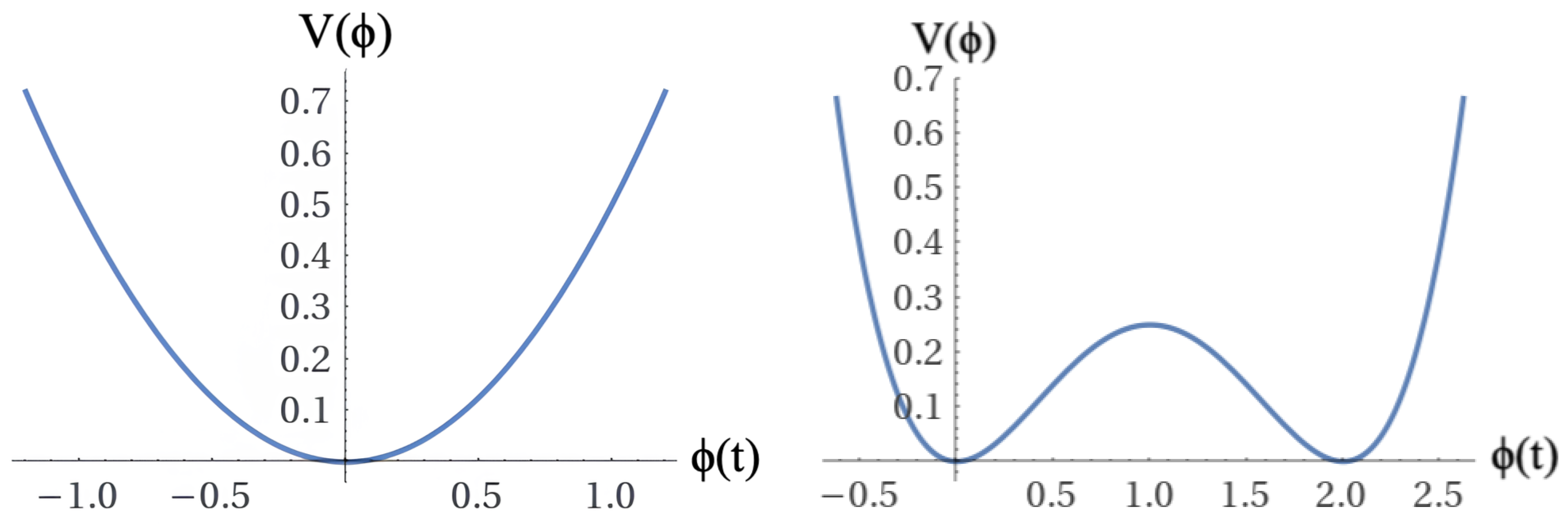
Figure 2.
The figure on the left shows an Argand-type plot of the distribution structure of real and imaginary sample solutions family of the wave equation (45) for the wave-function , sampling the conditions and . In the figures, the blue lines correspond to real parts while orange lines to imaginary components. The figures on the right show plots of sample individual solutions corresponding to the conditions on the top, and , below. For the figures, a mix of the naturalness short-range and fine-tuning long-range cosmological initial conditions was assumed with the set of values , , , , , , .
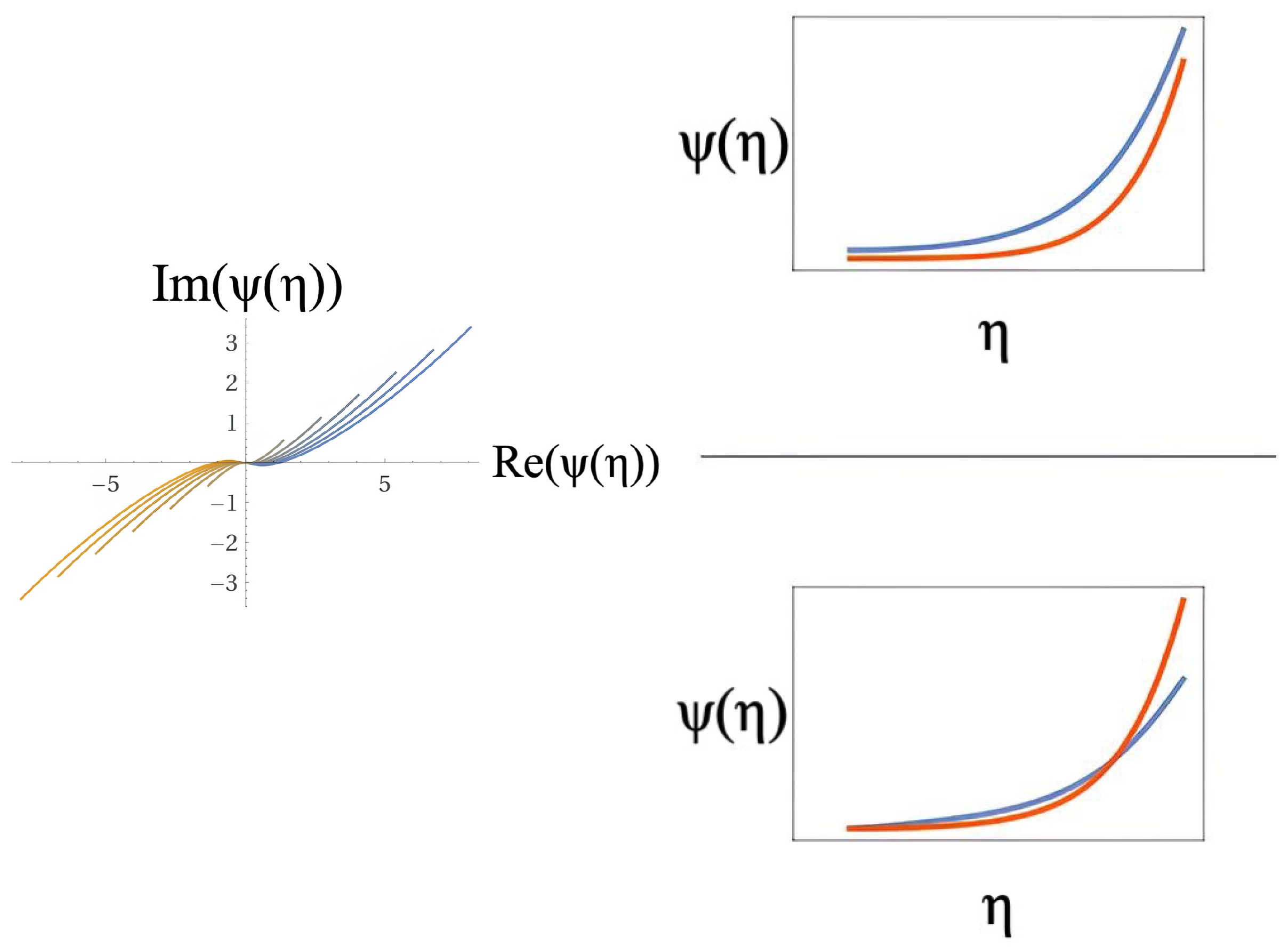
Figure 3.
Sample family solutions of the wave equation (45) for the wave-function assuming the fine-tuning set of the cosmological initial conditions: , , , , , , . The figure on the left shows an Argand-type plot depicting the structure of the distribution of real and imaginary sample solutions family of the wave-function , sampling the conditions and . The figures on the right show plots of sample individual solutions corresponding to the conditions on the top, and , below.

Figure 4.
On the left, sample solutions family of the wave equation (47) for the wave-function , sampling the conditions and and assuming and the naturalness condition. The figures on the right show plots of sample individual solutions corresponding to the conditions on the top, and , below.
Figure 4.
On the left, sample solutions family of the wave equation (47) for the wave-function , sampling the conditions and and assuming and the naturalness condition. The figures on the right show plots of sample individual solutions corresponding to the conditions on the top, and , below.
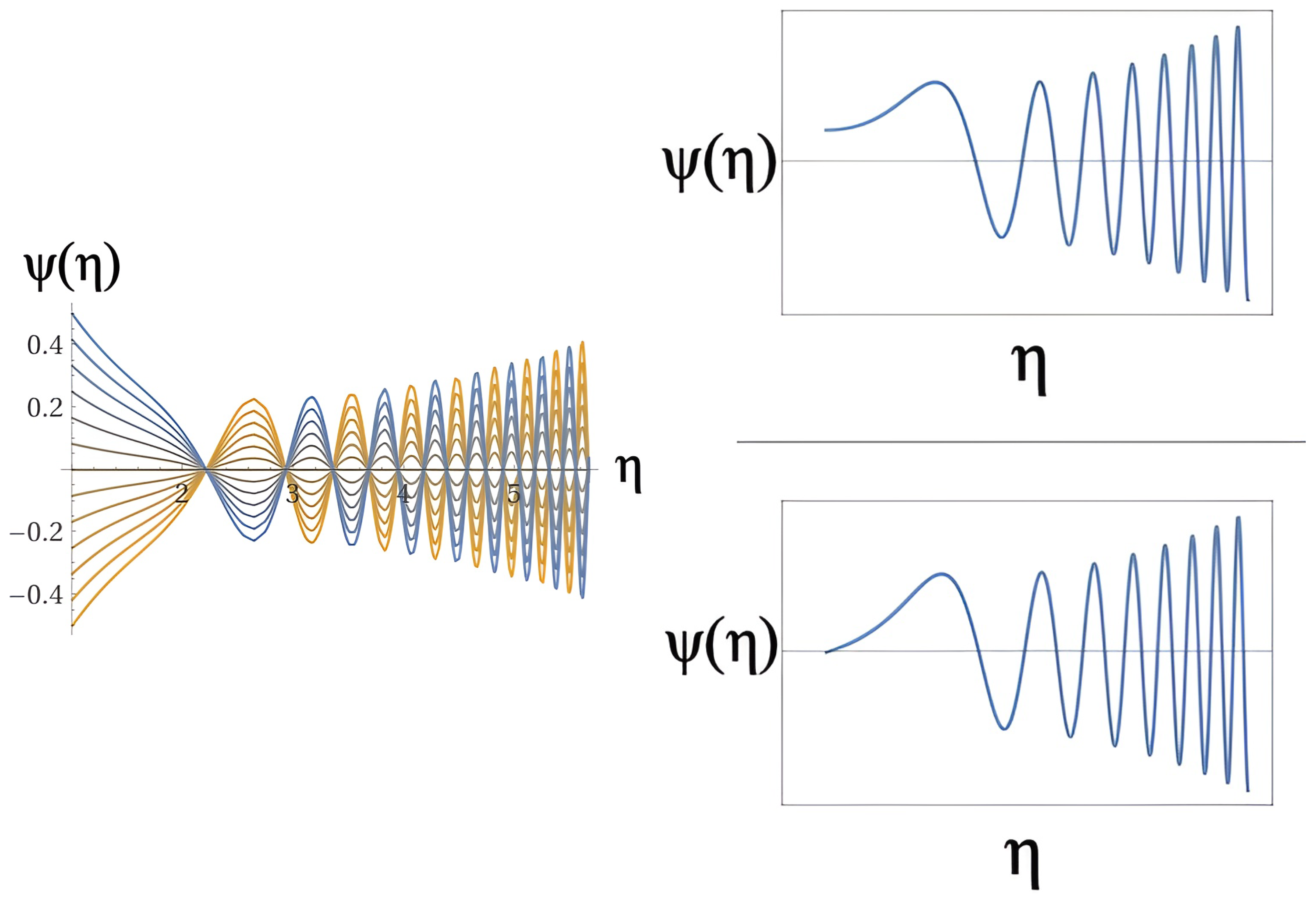
Figure 5.
Sample family solutions of equation (47) for the wave-function assuming the naturalness condition, and sampling the boundary conditions and . The upper-left and lower-left figures correspond respectively to the boundary conditions and . The upper-right and lower-right figures correspond respectively to the boundary conditions and .
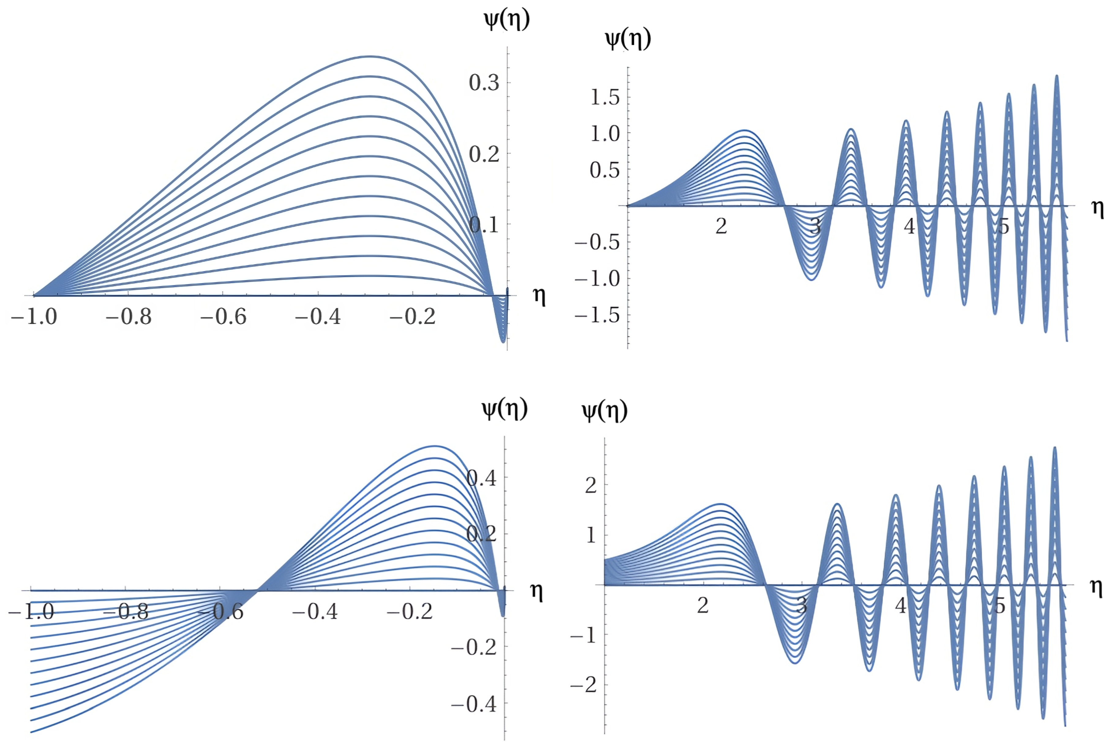
Figure 6.
Sample family solutions of the wave equation () for the wave-function , assuming the naturalness condition. The figure on the left shows an Argand-type plot of the cut distribution of real and imaginary numerical sample solutions of the wave-function . The figure on the right show plots of the solution of equation () given in (52). The blue lines correspond to real parts while orange lines to imaginary components.
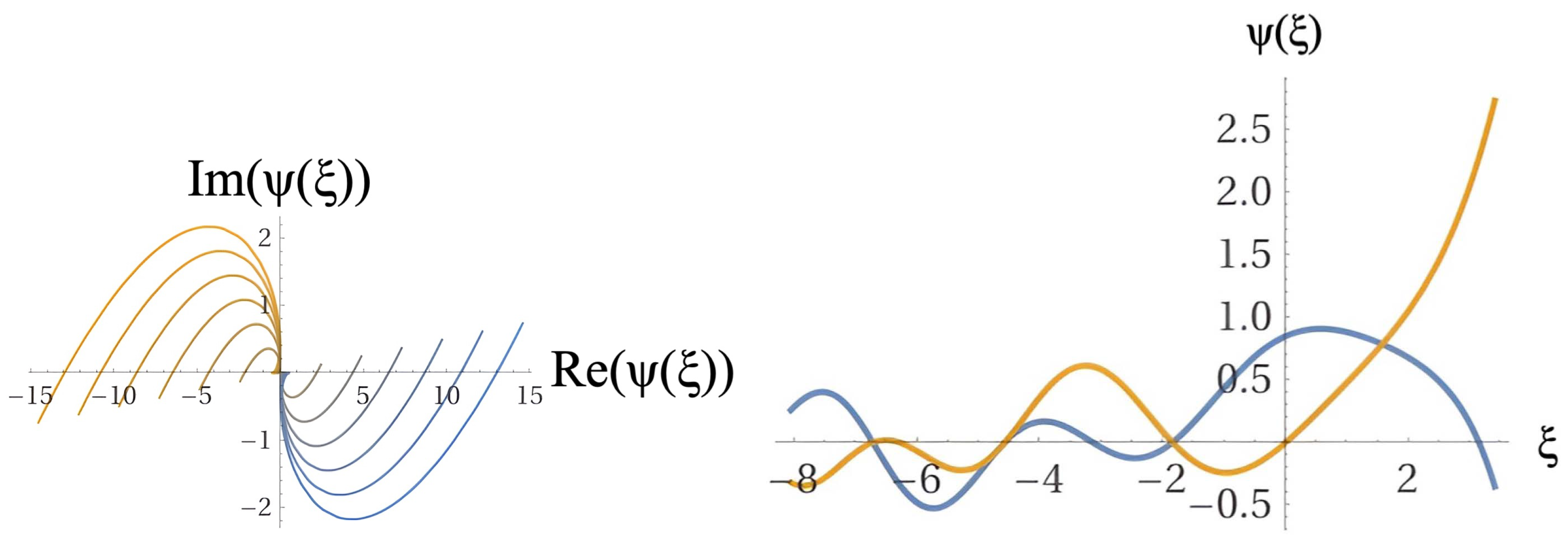
Figure 7.
Sample family solutions of the wave equation () for the wave-function , assuming the naturalness condition. The figure on the left corresponds to chaotic inflation while the figure on the right to non-chaotic inflation.
Figure 7.
Sample family solutions of the wave equation () for the wave-function , assuming the naturalness condition. The figure on the left corresponds to chaotic inflation while the figure on the right to non-chaotic inflation.
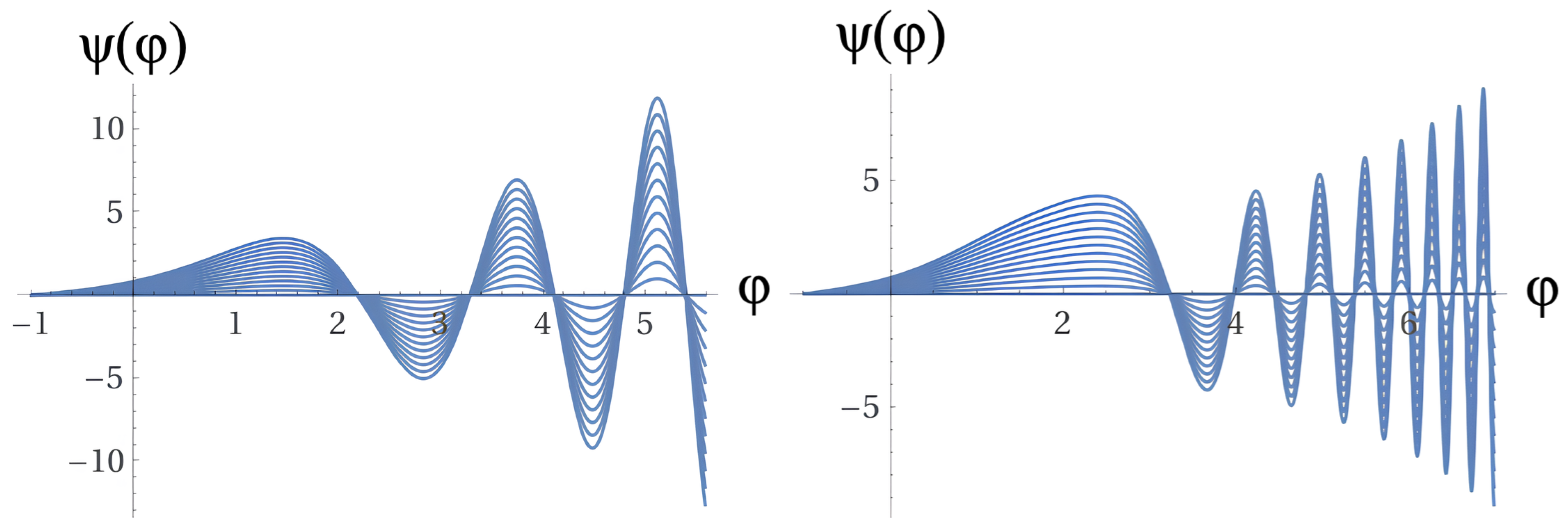
Table 1.
Assuming the perfect fluid radiation condition for the early Universe matter content, and the naturalness condition, the corresponding expressions for the coefficients (i = 1, ..., 6) are shown in the table. Making the quadratic terms explicit in equation (35) and combining similar terms, the coefficients comprise the parametric contributions.
Disclaimer/Publisher’s Note: The statements, opinions and data contained in all publications are solely those of the individual author(s) and contributor(s) and not of MDPI and/or the editor(s). MDPI and/or the editor(s) disclaim responsibility for any injury to people or property resulting from any ideas, methods, instructions or products referred to in the content. |
© 2025 by the authors. Licensee MDPI, Basel, Switzerland. This article is an open access article distributed under the terms and conditions of the Creative Commons Attribution (CC BY) license (http://creativecommons.org/licenses/by/4.0/).
Copyright: This open access article is published under a Creative Commons CC BY 4.0 license, which permit the free download, distribution, and reuse, provided that the author and preprint are cited in any reuse.


