Surface Temperature Prediction with Bayesian Structral Time Series

Madhavan Balasubramaniam

doi:10.20944/preprints202503.1175.v1

Submitted:

15 March 2025

Posted:

17 March 2025

You are already at the latest version

Abstract

This article develops a Bayesian Auto-Regressive forecasting model for predicting global surface temperatures and compares its performance with a frequentist approach. Using the NASA GISS Surface Temperature dataset, we first implement an AR(4) model and then incorporate trend and seasonality components. Results show that the Bayesian approach improves generalization and provides probabilistic parameter estimates, making it more robust for long-term forecasting.

Keywords:

Bayesian Time Series Forecasting

;

Auto-Regressive Models

;

Frequentist vs Bayesian Forecasting

;

Seasonality and Trend Analysis

;

PyMC

Subject:

Computer Science and Mathematics - Probability and Statistics

Introduction

Time series forecasting models aim to predict future values of a sequence based on its historical data. Prominent examples include ARIMA (AutoRegressive Integrated Moving Average), ES (Exponential Smoothing), and VAR (Vector AutoRegression) models. One of the characteristic of Time series model is the dependency on the previous time stamp. This is called Auto Correlation.

In this study, a Bayesian Auto-Regressive (AR) forecasting model is developed to predict future global surface temperature trends and is compared with its frequentist counterpart. The Bayesian AR model is first fitted to the data, followed by the incorporation of trend and seasonality components to enhance the accuracy of temperature predictions.

Literature Review

Bayesian Structural Time Series (BSTS) models have been widely applied across various industries for different forecasting and analytical applications. In [1], Brodersen et al. (2015) employed a BSTS state-space model to estimate the causal impact of market interventions, such as the effect of online advertising on search-related website visits. Their findings demonstrated that BSTS effectively quantifies causal impact in such scenarios. Poyser [2] utilized BSTS for forecasting Bitcoin’s market price and analyzing influencing parameters through seasonality trend decomposition. This approach provided valuable insights into Bitcoin price fluctuations. Qiu et al. [3] extended BSTS to a multivariate setting (MSBTS) to improve inference and prediction for multiple correlated time series. Their study applied MSBTS to stock market price data and Google search trends, demonstrating superior forecasting performance compared to the ARIMAX model, particularly when strong correlations exist among the time series. Díaz Olariaga et al. [4] showcased the effectiveness of BSTS in forecasting air traffic cargo demand in Colombia, highlighting its capability to model complex trends and seasonality. Similarly, Hamza and Mohammad [5] applied BSTS to predict Turkish coal production, reporting that BSTS outperformed ARIMA in predictive accuracy. Given the demonstrated efficacy of BSTS across diverse fields, its application can be extended to surface temperature prediction. The ability of BSTS to incorporate seasonality and external predictors makes it well-suited for climate-related time series modeling.

Dataset

Goddard Institute for Space Studies Surface Temperature Analysis Dataset [7] provides global surface temperature estimates based on meteorological station data, sea surface temperature data, and polar temperature estimates. The surface temperatures values are available from 1880. The model is trained the yearly average values of Surface Temperature from 1880 to 2005 and the temperature values of the last 20 years is predicted.

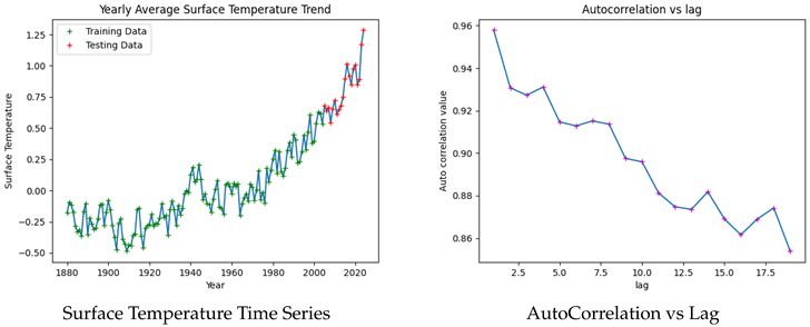
The figures illustrate a clear upward trend in surface temperature values, indicating a long-term increase. Additionally, a multi-year cyclic pattern with a periodicity of approximately seven years is observed, highlighting the presence of seasonality. The autocorrelation values for the first four lags exceed 0.93, suggesting a strong temporal dependence in the data.

These observations justify the use of an Auto-Regressive (AR) model incorporating trend and seasonality components. Given the high autocorrelation in the first four lags, an AR(4) model is initially fitted to the data.

AR (4) Model

Frequentist Approach:

In AR(4) model, the current observation

y_{t}

depends linearly on the previous 4 observations.

y_{t} = ρ_{0} + ρ_{1} y_{t - 1} + ρ_{2} y_{t - 2} + ρ_{3} y_{t - 3} + ρ_{4} y_{t - 4} + ϵ_{t}

where,

\begin{matrix} y_{t - 1}, y_{t - 2}, y_{t - 3}, y_{t - 4} & : the previous 4 observations \\ ρ_{1}, ρ_{2}, ρ_{3}, ρ_{4} & : auto - regressive coefficients \\ ρ_{0} & : the constant term \\ ϵ_{t} & : error term (white noise) \end{matrix}

The dataset is first standardized to ensure comparability between the frequentist and Bayesian approaches. An Auto-Regressive (AR) model of order 4 is then implemented, with the lag parameter set to four. The model coefficients are estimated by optimizing the likelihood function, minimizing the sum of squared errors between the predicted values

{\hat{y}}_{t}

and the observed values

y_{t}

. Once the model is fitted, it is used to generate future predictions based on the estimated parameters.

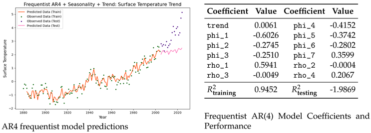
Frequentist AR(4) Model: Coefficients and Performance :

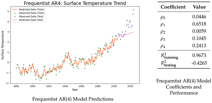
The coefficient of determination (

R^{2}

) measures how well the independent variables in the model explains the variation in the dependent variable. A higher

R^{2}

value indicates a better fit to the data. Although the Auto-Regressive (AR) model demonstrates a strong fit to the training dataset (

R_{training}^{2} = 0.9673

), it fails to generalize well to the testing data, resulting in a negative

R^{2}

value (

R_{testing}^{2} = - 0.4265

). This suggests that the model overfits the training data and is unable to capture the upward trend in the test dataset. This is evident from the model predictions illustrated above.

Bayesian Approach:

The Bayesian Auto Regressive Model of order 4 is described as follows:

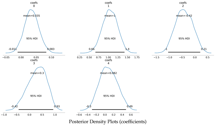
\begin{matrix} Prior on Coefficients : ρ_{j} & \sim N (μ = 0, σ = 10), j = 0, 1, 2, 3, 4, \\ Prior on σ_{c} : σ_{c} & \sim E xp (λ = 1), \\ Likelihood : y_{t} ∣ ρ_{j}, y_{t - j} & \sim N (μ = ρ_{0} + \sum_{j = 1}^{4} ρ_{j} y_{t - j}, σ = σ_{c}) . \end{matrix}

Since prior information on the coefficients is not available, a non-informative prior is assigned. Specifically, a normal distribution with mean 0 and standard deviation 10 is used for the five coefficients, while an exponential distribution with a mean of 1 is assigned to

σ

. The exponential prior is weakly informative, favoring smaller values of

σ

.

Using Bayes’ theorem, these priors are updated based on the observed time-series data to obtain the posterior distributions of the coefficients and

σ_{c}

. Unlike point estimates derived from the frequentist approach, these posterior distributions provide a comprehensive probabilistic characterization of the parameters.

For forecasting future values, samples are drawn from the posterior distributions of the coefficients and

σ_{c}

. These samples are then used to iteratively simulate future

y_{t}

values, thereby generating a posterior predictive distribution for the forecasted values.

Posterior stats of coefficients:

Parameter	Mean	SD	HDI 2.5%	HDI 97.5%	$\hat{R}$
coefs[0]	0.035	0.024	-0.012	0.082	1.0
coefs[1]	1.035	0.195	0.657	1.413	1.0
coefs[2]	-0.392	0.339	-1.008	0.254	1.0
coefs[3]	0.268	0.376	-0.452	0.962	1.0
coefs[4]	0.100	0.212	-0.304	0.498	1.0
sigma	0.253	0.019	0.216	0.291	1.0

Forecasting with Bayesian AR4 model

During forecasting, the model predicts future values based on past observations. The number of steps for prediction must be specified. Since the autoregressive process of order 4 (AR(4)) requires an initial distribution, it is constrained to the last four observations of the training data. To enforce this constraint, a Dirac delta distribution of order 4 is employed, placing four point masses at the most recent observations. The posterior distribution of the coefficients is then utilized to derive the predictive distribution of future values.

Posterior density plots of coefficients :

For the Bayesian AR(4) model, the coefficient of determination (

R^{2}

) is estimated as 0.88 for the training set and 0.171 for the testing set. In contrast, the frequentist approach yields

R^{2}

values of 0.9673 and -0.4265 for training and testing, respectively. These results indicate that the Bayesian approach mitigates overfitting, providing more generalizable predictions. The predicted values are now compared with the actual observations from the testing dataset to evaluate the forecasting performance.

Forecasting with Bayesian AR4 model

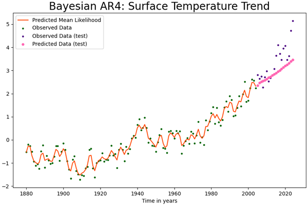
The figure illustrates that the predicted values closely follow the observed values, demonstrating improved performance compared to the frequentist approach. However, the model fails to capture the steep trend present in the actual data. Additionally, the seasonal and cyclic variations are not well represented.

To address these limitations, seasonal and cyclic components are incorporated into the Bayesian AR(4) model to enhance its predictive accuracy.

AR (4) Model with trend and seasonality

Frequentist Approach :

In AR(4) Trend Seasonality model, the current observation

y_{t}

depends linearly on the previous 4 observations, its sequence number t, and the seasonal terms. The seasonal terms consist of observations ’kp’ steps before, where k ranges from 1 to m.

y_{t} = ρ_{0} + \sum_{j = 1}^{4} ρ_{j} y_{t - j} + \sum_{k = 1}^{m} ϕ_{k} y_{t - k p} + α \cdot t + ϵ_{t}

where,

\begin{matrix} ρ_{1}, ρ_{2}, ρ_{3}, ρ_{4} & : Auto regressive coefficients \\ ϕ_{k} & : seasonality coefficients \\ α \cdot t & : trend \\ p & : Period of seasonality \end{matrix}

To model the seasonality and trend with AutoRegression (4), seasonality is incorporated by introducing dummy variables corresponding to each period within the seasonal cycle, while the trend is captured through a steady increase over time. By visual inspection, periodicity of the time series is estimated to be 7, corresponding to 7 dummy variables. The coefficients of autoregression, trend, and seasonal components are estimated by minimizing the sum of squared errors between the predicted values

{\hat{y}}_{t}

and the observed values

y_{t}

, yielding maximum likelihood estimates. The fitted model can then be used to generate future predictions based on these estimated parameters.

The model outperforms the AR(4) frequentist model, achieving a higher

R^{2}

on the testing data and effectively capturing the cyclic patterns. However, it fails to forecast the upward trend in the testing data, as indicated by the very small trend coefficient of

0.0061

. Bayesian Approach:

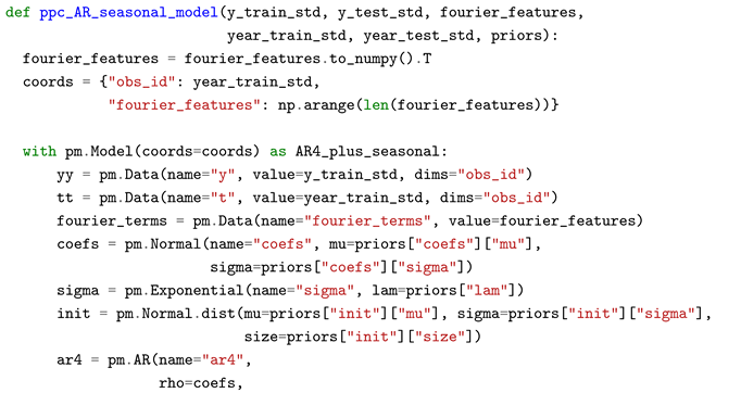
The Bayesian AR(4) model with trend and seasonality is described as follows.

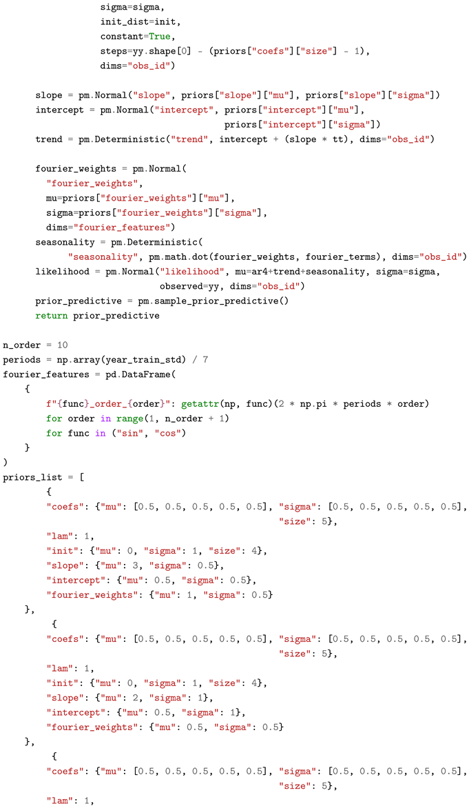
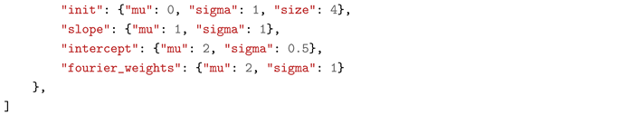
$\begin{matrix} Prior on AR coefficients : & ρ_{j} \sim N (0.5, 0.5), j = 0, 1, 2, 3, 4, \\ Prior on slope coefficient : & β \sim N (3, 0.5), \\ Prior on intercept : & α \sim N (0.5, 0.5), \\ Prior on σ_{c} : & σ_{c} \sim Exp (1), \\ Prior on Fourier weights : & fw \sim N (1, 0.5), \\ Trend (deterministic) : & trend = α + β \cdot t, \\ Seasonality (deterministic) : & seas = fw \cdot fourier_features, \\ Likelihood : y_{t} ∣ ρ_{j}, y_{t - j} & \sim N (ρ_{0} + \sum_{j = 1}^{4} ρ_{j} y_{t - j} + seas + trend, σ_{c}) \end{matrix}$

For effective MCMC sampling, when more degrees of freedom (such as trend and seasonality) are added, the Bayesian model requires a more informative prior. Since we know that the AR coefficients typically lie within [0,1], a prior of N(0.5,0.5) provides reasonable flexibility while discouraging values outside this range.

Moreover, as mentioned in [6], the Bayesian AR model with trend struggles to capture the trend line when using highly uninformative priors. Therefore, increasing the variability will never capture the directional pattern in the data. Hence, informative priors for the slope and intercept were chosen by iterating over multiple candidates using the method of prior predictive check.

Trend: Bayesian AR(4) model exhibited a better upward trend compared to its frequentist counterpart. However, the trend eventually died out, and the predictions converged to the mean value when additional steps were forecasted. Adding a trend structure to the model would resolve this issue.

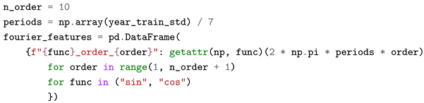
Seasonality: To account for seasonal cyclic patterns, synthetic Fourier features are generated and incorporated into the model. This approach represents the data as a weighted combination of sine and cosine functions. The cyclic components are treated as regular feature variables in the regression framework. Since these features are essential for capturing periodic trends, the model also requires Fourier features during the prediction phase

Prior Predictive check:

In a prior predictive check, the model computes the possible values of the observed variables (likelihood function). It converts the choices made in the parameter space to the observed values. Thinking in terms of observations rather than coefficients makes the prior evaluation easier. Hence, the prior predictive check helps us choose reasonable priors.

Prior Predictive Check for AR4 + seasonality + trend model

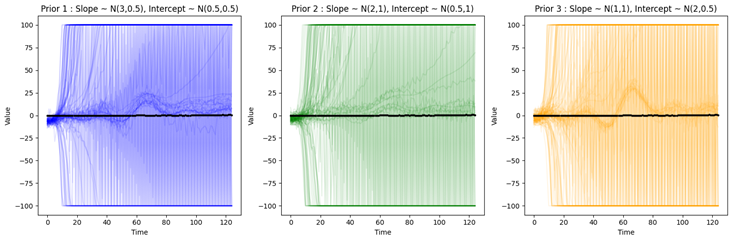
Before performing prior predictive checks on various candidate priors for the slope, intercept, and Fourier coefficients, the remaining prior distributions were frozen.

Observations :

Most of the processes in three of the priors quickly diverge to large values. This is due to the recursive nature of the auto regressive MCMC sampling process.

In the second prior, most samples quickly diverge to large values, and only weak cyclic patterns are visible. However, there is an upward trend, which is desirable.

The amplitude of the cyclic patterns are too large in the third prior. The first prior exhibits both a cyclic pattern and a weak upward trend. Therefore, it is a suitable candidate prior for Bayesian AR4 + seasonality + trend model.

Posterior stats of Bayesian AR(4)+ST model coefficients:

Parameter	Mean	SD	HDI 2.5%	HDI 97.5%	$\hat{R}$
coefs[0]	-0.035	0.035	-0.105	0.032	1.0
coefs[1]	1.299	0.169	0.964	1.618	1.0
coefs[2]	-0.085	0.343	-0.741	0.573	1.0
coefs[3]	0.055	0.339	-0.606	0.711	1.0
coefs[4]	-0.295	0.162	-0.611	0.013	1.0
sigma	0.289	0.022	0.248	0.332	1.0
slope	2.013	0.438	1.186	2.891	1.0
intercept	0.870	0.485	-0.072	1.834	1.0

Posterior density plots of coefficients, slope, trend:

R^{2}

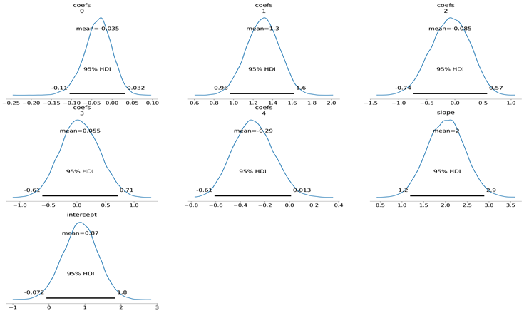
score obtained on training data and testing data are 0.8634 and 0.7184, a significant improvement over the previous models.

Forecasting with Bayesian AR4 model with Seasonality and Trends:

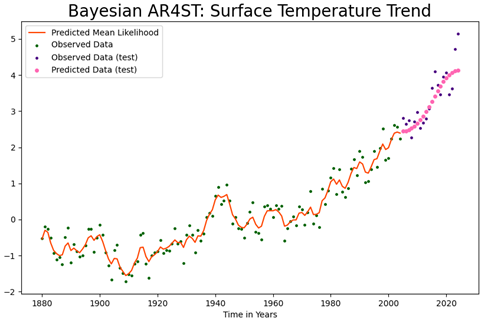
We can observe that the model is able to capture both the seasonal variations and the trend in the data and able to forecast accurate values for the surface temperature

Model Comparison

Model	$R_{train}^{2}$	$R_{test}^{2}$
Frequentist AR(4)	0.9673	-0.4265
Bayesian AR(4)	0.8800	0.1710
Frequentist AR(4) + Seasonality + Trend	0.9452	-1.9870
Bayesian AR(4) + Seasonality + Trend	0.8634	0.7184

Conclusions

This study systematically analyzed the performance of Frequentist and Bayesian autoregressive models. Initially, under the assumption of uninformative priors, the Bayesian AR(4) model was expected to perform on par with its Frequentist counterpart. However, empirical results demonstrated that the Bayesian AR(4) model exhibited superior predictive accuracy.

Extending the analysis, the Frequentist AR(4)+ST model was employed to capture cyclic patterns. While this model effectively identified periodic variations, it failed to account for the underlying trend, highlighting a fundamental limitation in its formulation.

To address this, we incorporated weakly informative priors into the Bayesian AR(4)+ST model and conducted prior predictive checks to refine the selection of priors for slope, trend, and Fourier coefficients. This approach significantly enhanced the model’s ability to capture both cyclical and trend components, leading to a marked improvement in predictive performance. The

R^{2}

metric was used as a comparative measure, further validating the superiority of the Bayesian framework.

Beyond predictive accuracy, Bayesian AR models offer a distinct advantage by providing posterior distributions for both model coefficients and predicted variables, allowing for a more comprehensive uncertainty quantification. This probabilistic characterization enhances interpretability and robustness, making Bayesian methods a compelling choice for time series modeling in complex real-world scenarios.

Appendix A

Code Implementation Frequentist AR(4) Model

The AutoReg class from the statsmodels library is used to model AutoRegression (4) in Python with lags set to 4. The .fit() method estimates coefficients by maximizing the likelihood and minimizing the sum of squared errors. Future predictions are made using the .predict() method.

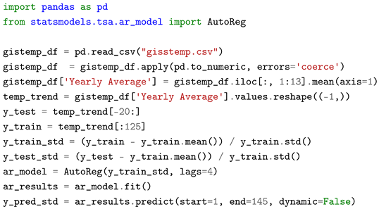Code Implementation Bayesian AR(4) Model

Modelling in PyMC:

To obtain the posterior estimates, the model is set up in PyMC using the pm.AR() module, which is defined as the mean of the likelihood function. Each lag term requires an initialization distribution, for which a normal distribution with a mean of 0 and a standard deviation of 10 is used.

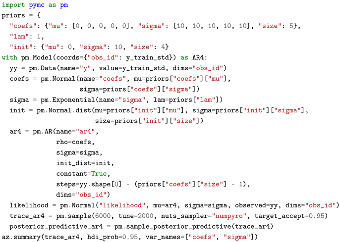Forecasting Step:

During forecasting, the model predicts future values based on trained past data, requiring a specified forecast horizon. The AR(4) process depends on an initial distribution constrained to the last four observations of

y_{train}

. A Dirac Delta distribution of order four, with point masses at these observations, is used to model this constraint.

Forecasting Step Python Code:

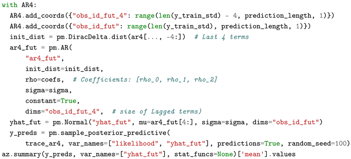Code Implementation - Frequentist AR(4) Model with Trend and Seasonality

To model seasonality and trend with AutoRegression (4), the seasonal argument in the AutoReg class is set to true, period to 7, trend to ’t’ (time trend only), and lags to 4. Estimates for the autoregression, trend, and seasonality coefficients are obtained using the .fit() method, which employs an optimization algorithm to minimize the sum of squared errors between the predicted values

{\hat{y}}_{t}

and the observed values

y_{t}

, producing maximum likelihood estimates (MLEs). Future predictions are generated using the .predict() method.

Python Implementation

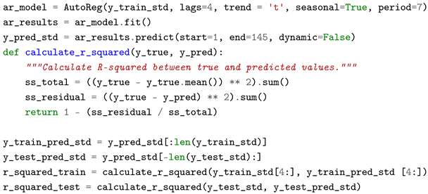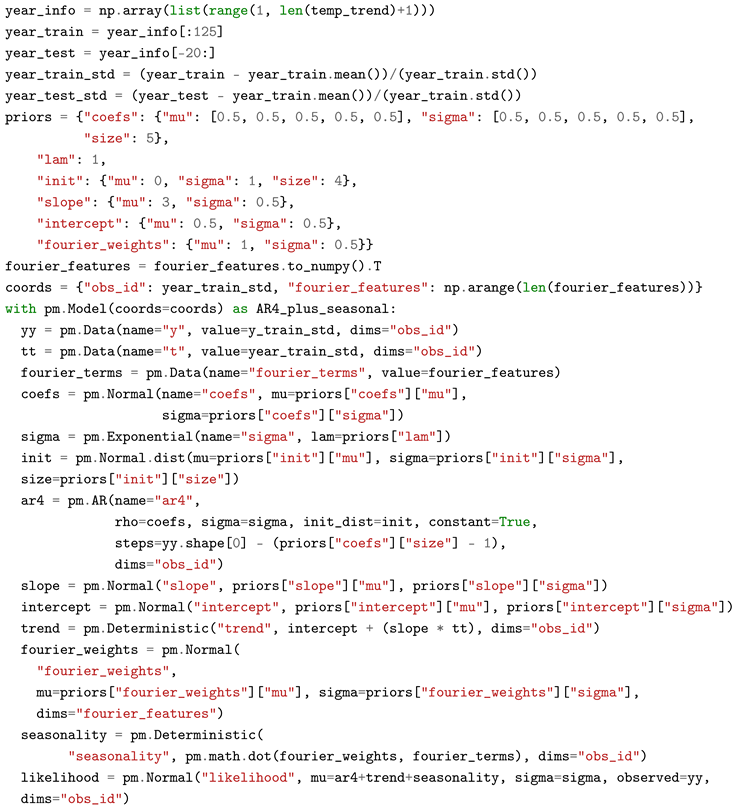
Code Implementation Bayesian AR(4) Model with Trend and Seasonality

Code to generate fourier features:

Code for prior predictive check

Modelling in PyMC:

The priors for the slope, intercept, and Fourier weights are specified, followed by the computation of trend and seasonality as deterministic components. These components are integrated into the autoregressive process, with their sum serving as the mean of the likelihood function. Once the posterior distributions are estimated, forecasting is performed using Fourier features for the testing period.

Bayesian AR(4) Model with seasonality and trend:

Forecasting with Bayesian AR(4) Model with seasonality and trend:

References

K. H. Brodersen, F. K. H. Brodersen, F. Gallusser, J. Koehler, N. Remy, and S. L. Scott, “Inferring causal impact using Bayesian structural time-series models,” Annals of Applied Statistics, vol. 9, no. 1, pp. 247-274, Mar. 2015. [CrossRef]
O. Poyser, “Exploring the determinants of Bitcoin’s price: an application of Bayesian Structural Time Series,” 2017. [CrossRef]
J. Qiu, S. R. J. Qiu, S. R. Jammalamadaka, and N. Ning, “Multivariate Bayesian structural time series model,” Journal of Machine Learning Research, vol. 19, no. 68, pp. 1-33, 2018.
Y. Rodríguez and O. Díaz Olariaga, “Air Traffic Demand Forecasting with a Bayesian Structural Time Series Approach,” Periodica Polytechnica Transportation Engineering, vol. 52, no. 1, pp. 75–85, 2024. [CrossRef]
H. A. Hamza and M. J. Mohammad, “A Comparison of the Bayesian Structural Time Series Technique with the Autoregressive Integrated Moving Average Model for Forecasting,” Migration Letters, vol. 21, no. S4, pp. 528–538, 2024. [CrossRef]
N. Forde, “Forecasting with Structural AR Time Series,” in PyMC Examples, edited by PyMC Team. [CrossRef]
GISTEMP Team, “GISS Surface Temperature Analysis (GISTEMP), version 4,” NASA Goddard Institute for Space Studies, Dataset accessed 2024-12-01. Available: https://data.giss.nasa.gov/gistemp/.
E. Herbst and C. Fonnesbeck, “Analysis of An Model in PyMC,” in PyMC Examples, edited by PyMC Team. [CrossRef]

Disclaimer/Publisher’s Note: The statements, opinions and data contained in all publications are solely those of the individual author(s) and contributor(s) and not of MDPI and/or the editor(s). MDPI and/or the editor(s) disclaim responsibility for any injury to people or property resulting from any ideas, methods, instructions or products referred to in the content.

© 2025 by the authors. Licensee MDPI, Basel, Switzerland. This article is an open access article distributed under the terms and conditions of the Creative Commons Attribution (CC BY) license (http://creativecommons.org/licenses/by/4.0/).

Copyright: This open access article is published under a Creative Commons CC BY 4.0 license, which permit the free download, distribution, and reuse, provided that the author and preprint are cited in any reuse.

Surface Temperature Prediction with Bayesian Structral Time Series

Abstract

Keywords:

Subject:

Introduction

Literature Review

Dataset

AR (4) Model

Frequentist Approach:

Frequentist AR(4) Model: Coefficients and Performance :

Bayesian Approach:

Posterior stats of coefficients:

Forecasting with Bayesian AR4 model

Posterior density plots of coefficients :

Forecasting with Bayesian AR4 model

AR (4) Model with trend and seasonality

Frequentist Approach :

Prior Predictive check:

Prior Predictive Check for AR4 + seasonality + trend model

Observations :

Posterior stats of Bayesian AR(4)+ST model coefficients:

Posterior density plots of coefficients, slope, trend:

Forecasting with Bayesian AR4 model with Seasonality and Trends:

Model Comparison

Conclusions

Appendix A

Code Implementation Frequentist AR(4) Model

Code Implementation Bayesian AR(4) Model

Code Implementation - Frequentist AR(4) Model with Trend and Seasonality

Code Implementation Bayesian AR(4) Model with Trend and Seasonality

References

MDPI Initiatives

Important Links

Subscribe