Dynamic Learning Models for Adaptive Digital Twins: A Scalable Approach to Real-Time Adaptability in Non-Stationary Environments

1. Introduction

Digital twin technology has emerged as a key paradigm for integrating real-time data with high-fidelity models of physical systems. A digital twin (DT) is generally defined as a digital model of a specific physical asset that remains in sync with the asset throughout its lifecycle [1,2]. In other words, a DT is a living model that is continuously updated to reflect changes in its physical counterpart. The concept originated in the aerospace industry, where NASA introduced the idea of a “digital twin” around 2010 as a means to improve spacecraft simulations [3,4]. One early formalization described a digital twin as:

“an integrated multiphysics, multiscale, probabilistic simulation of an as-built vehicle that uses physical models, sensor updates, and history to mirror the life of its corresponding flying twin”.

[5,6]

This highlights that a true digital twin must be dynamically linked to data from the physical system.

An important distinguishing feature of digital twins, as opposed to traditional offline simulations, is adaptivity. According to a recent data science perspective, a digital twin can be viewed as an open dynamical system with an updating mechanism, essentially a complex adaptive system that generates simulation data indistinguishable from the physical system [7,8]. This adaptivity allows the twin to evolve along with the real system, enabling capabilities such as real-time monitoring, predictive diagnostics, and decision support [9,10]. However, designing such adaptive digital twins (ADT) raises fundamental questions:

• How should the twin’s model update itself based on streaming data?
• Will these updates converge to an accurate representation of the physical system?
• What are the theoretical limits on the twin’s fidelity and stability?

In this paper, we address these questions by developing a mathematical framework for adaptive digital twins with a focus on theoretical guarantees. We define the concept of an adaptive digital twin rigorously and propose an algorithmic approach for online learning of the twin model. We then analyze the convergence properties of this adaptation scheme, deriving conditions for stability and convergence in the presence of uncertainties.

Our contributions are summarized as follows:

• We formalize the definition of an Adaptive Digital Twin (ADT) as a digital twin endowed with mechanisms to update its state or parameters continuously using live data. This formal definition (Section 3) clarifies the difference between a static model and a truly adaptive twin.
• We present a mathematical model for the coupled physical-digital system, including notation for the physical system dynamics and the digital twin dynamics. Based on this model, we introduce an online learning algorithm for the ADT that assimilates new observations and adjusts the twin’s parameters in real-time (Section 4). The algorithm is described in pseudocode (Algorithm 1) with step-by-step updates for implementation.
• We derive theoretical results on convergence and stability. In particular, under assumptions such as observability of the physical system and sufficient excitation in the data, we prove that the adaptive updates drive the twin’s state to track the physical system’s state asymptotically (Section 5). The main result (Theorem 2) provides a convergence guarantee for the parameter estimation error. We also discuss the rate of convergence and how it depends on design parameters (e.g., learning rates).
• We investigate theoretical limits and trade-offs. Even with an optimal design, factors like model mismatch, measurement noise, and time delays can impose lower bounds on the accuracy of a digital twin. We provide analysis of these limits in Section 5.2, including an example of a scenario where the twin cannot perfectly converge due to unobservability. A formal proposition is given to illustrate how noise leads to an error floor in estimation.
• We include a case study illustration (Section 6) to demonstrate the application of the proposed framework. In this illustrative example, we consider a simple physical system (a second-order dynamic system) and show how the adaptive twin tracks it. We present a table summarizing the effect of different adaptation rates on convergence speed and accuracy (Table 4).

The remainder of this paper is organized as follows. Section 2 reviews related work and situates our contributions in the context of existing research on digital twins. Section 3 introduces the mathematical framework and formal definitions. Section 4 describes the adaptive twin algorithm in detail. Section 5 presents the theoretical convergence analysis and proofs. Section 5.2 discusses the fundamental limits and provides additional insights (including a brief discussion on computational complexity and real-time constraints). Section 6 provides an illustrative example. Finally, Section 7 concludes the paper and outlines future research directions.

2. Background and Related Work

The concept of digital twins has evolved rapidly in recent years, finding applications in manufacturing, energy systems, healthcare, and urban infrastructure. Several survey papers and reviews (e.g., [1,3]) trace this evolution from its initial conceptualization to modern implementations. Here, we focus on the aspects most relevant to adaptive digital twins, particularly online model updating, data assimilation, and theoretical analyses of twin models.

2.1. Digital Twin Foundations

The term Digital Twin was popularized by NASA and the U.S. Air Force as part of vehicle health management for aerospace systems [1]. Glaessgen and Stargel [1] outlined the digital twin paradigm as a high-fidelity model synchronized with a physical asset, emphasizing its potential for life-cycle monitoring. Since then, various definitions have been proposed. A common theme is the integration of three key elements: the physical asset, its virtual model, and the data connections that ensure synchronization. An often-cited perspective defines a digital twin as comprising a physical product, a virtual counterpart, and real-time data flows between them.

[5] have emphasized that achieving robust digital twins at scale requires rigorous mathematical foundations. Key challenges include model stability, uniqueness of solutions, and convergence of coupled simulations. If the combined physical-digital system does not yield stable and convergent behavior, the digital twin will not remain valid over time [7]. These observations motivate the need for a strong theoretical analysis of adaptive digital twins.

2.2. Defining System Non-Stationarity

Real-world systems often exhibit non-stationary behavior due to environmental changes, aging components, and dynamic operating conditions. In an adaptive digital twin, non-stationarity poses a fundamental challenge: the twin’s model must continuously track and update its internal representation to match the evolving physical system.

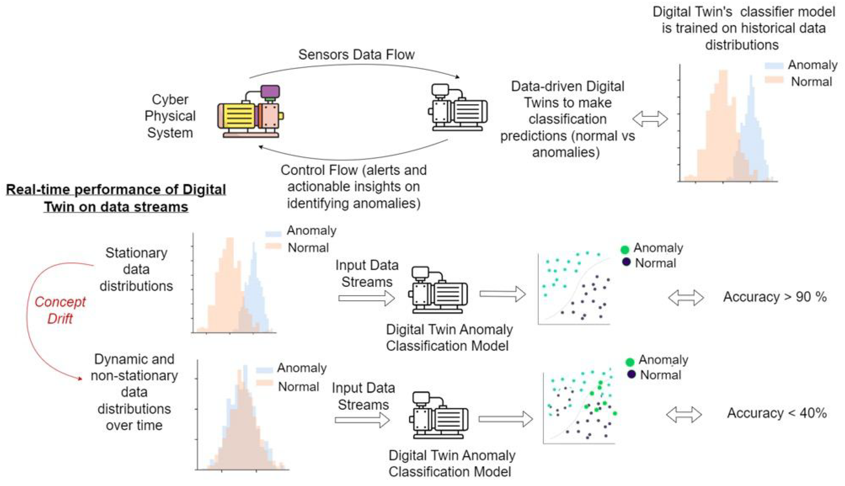
Figure 1. Real-time performance of a digital twin’s anomaly classification model under concept drift (distribution shift). Initially, the model is trained on stationary data and achieves high accuracy. As the environment evolves and data distributions shift over time, the decision boundary becomes misaligned, causing accuracy to drop drastically (e.g., from >90% to <40%). This illustrates the need for continual adaptation in digital twins to maintain performance under changing conditions.

Figure 1. Real-time performance of a digital twin’s anomaly classification model under concept drift (distribution shift). Initially, the model is trained on stationary data and achieves high accuracy. As the environment evolves and data distributions shift over time, the decision boundary becomes misaligned, causing accuracy to drop drastically (e.g., from >90% to <40%). This illustrates the need for continual adaptation in digital twins to maintain performance under changing conditions.

To formally characterize non-stationary environments, we define them in terms of evolving probability distributions. In a stationary setting, the system’s dynamics—such as state transition probabilities and reward distributions in a Markov Decision Process (MDP)—are fixed over time. In contrast, a non-stationary environment is one where the transition function $P_t$ and/or reward function $R_t$ change over time due to evolving external conditions, control policies, or underlying system variations.

Mathematical Definition of Non-Stationarity

At each discrete time step t, the environment can be represented as a time-dependent MDP:

$${\mathcal{M}}_t=\langle S,A,P_t,R_t\rangle ,$$

(1)

where:

• S is the state space,
• A is the action space,
• $P_t\left(s^{\prime }\right|s,a)$ is the time-dependent state transition probability,
• $R_t(s,a)$ is the time-dependent reward function.

A common approach to handling non-stationarity is to assume that variations are bounded within a variation budget, which measures the total change over a given time horizon T.

Variation Budgets for Transition and Reward Dynamics

Reward variation budget:

$$B_r=\sum _{t=1}^{T-1}\underset{s\in S,a\in A}{max}\left|R_{t+1}(s,a)-R_t(s,a)\right|.$$

(2)

Transition variation budget:

$$B_p=\sum _{t=1}^{T-1}\underset{s\in S,a\in A}{max}\parallel P_{t+1}(·|s,a)-P_t(·|s,a){\parallel }_1.$$

(3)

These bounds, $B_r,B_p\ge 0$, quantify how far the environment deviates from stationarity. If $B_r=B_p=0$, the environment is fully stationary.

Types of Non-Stationarity

Non-stationary behavior in digital twins can be categorized based on the nature of changes in $P_t$ and $R_t$:

• Gradual Drift: Slow, continuous changes in system dynamics over time [11,12].
• Piecewise-Constant Dynamics: Transition and reward functions remain constant for intervals but shift at unknown breakpoints.
• Adversarial or Unstructured Changes: The environment shifts arbitrarily within predefined variation budgets [13,14].

Implications for Digital Twins

For digital twins, non-stationary environments arise due to:

• Component Wear and Degradation: Physical components degrade over time, leading to changes in system parameters.
• Changing Operating Conditions: Variations in temperature, pressure, or load conditions affect system behavior.
• Sensor Recalibration: Shifts in measurement characteristics require continuous model re-alignment.
• External Perturbations: Unexpected disturbances, such as environmental shocks, alter the twin’s input-output mapping.

Connections to Concept Drift and Non-Stationary RL

The above issues relate closely to the concept drift problem in machine learning, where the statistical relationship between input and output data evolves over time. Concept drift is a significant challenge in data-driven adaptive digital twins and is commonly categorized as:

• Gradual Drift: Sensor readings slowly change due to wear and tear.
• Abrupt Drift: A sensor recalibrates suddenly, altering all subsequent measurements.
• Recurring Drift: Periodic or seasonal variations in system behavior.

Several non-stationary reinforcement learning (RL) algorithms have been proposed to address this issue. Recent work by Cheung et al. [14] and Wei et al. [15] explores adaptive regret minimization in environments with continuously evolving reward functions, while Finn et al. [16,17] demonstrate meta-learning techniques that accelerate adaptation in dynamic settings.

Theoretical Guarantees for Adaptive Digital Twins

The ability of a digital twin to successfully track a non-stationary system depends on:

• Observability: The system must provide enough information for the twin to infer its state accurately.
• Persistence of Excitation: The system must receive sufficiently diverse inputs to enable accurate parameter updates.
• Convergence of the Adaptive Update Law: Stability of parameter updates must be ensured using Lyapunov-based stability analysis [18,19].

Formal Definition of a Non-Stationary Digital Twin

We formally define a non-stationary adaptive digital twin as one in which either the transition dynamics $P_t$ or the reward/output distribution $R_t$ is explicitly time-dependent. Equivalently, the joint probability distribution of states, actions, and rewards:

$$P_t(s_{t+1},r_t|s_t,a_t)$$

(4)

is not identical for all t. This definition provides a rigorous foundation for analyzing digital twin adaptation algorithms under different types of non-stationarity.

2.3. Theoretical Foundations of Adaptation

Several works have explored adaptive learning in dynamic environments, providing a foundation for digital twin adaptation. For example [13] introduced a framework for stochastic bandits with non-stationary rewards, analyzing regret minimization with variation budgets. Their results establish fundamental bounds for learning in changing environments.

In reinforcement learning, [14,20] extended regret analysis to non-stationary MDPs, showing that policy adaptation can achieve sublinear regret under certain conditions. More broadly, Padakandla [21] surveyed various reinforcement learning approaches for dynamically varying environments, situating adaptive digital twins within this context.

From a control-theoretic perspective, adaptive control stability has been extensively studied. Classical works by Narendra and Annaswamy [18], along with more recent studies by Janakiraman et al. [22], establish Lyapunov stability criteria for learning in dynamic settings. These results provide rigorous guarantees for parameter adaptation in digital twins.

Finally, concept drift adaptation has been widely explored in the data stream mining community. [11] surveyed techniques for detecting and handling distributional shifts, which are directly relevant to real-time digital twin updates. Recent applied work, such as [23], demonstrates practical implementations of adaptive twins for IoT anomaly detection.

2.4. Meta-Learning and Rapid Adaptation

Meta-learning techniques have been proposed to accelerate adaptation in changing environments. [16,17] formalized Model-Agnostic Meta-Learning (MAML), which allows models to quickly fine-tune to new conditions with minimal data. [24] extended meta-learning to continuous adaptation scenarios, further strengthening its applicability to digital twins.

Accelerating Adaptation with Meta-Learning

Traditional adaptive learning methods rely on accumulating sufficient data before updating models, making them slow in highly dynamic environments. Meta-learning, by contrast, learns how to adapt, allowing a model to generalize across different tasks with few gradient steps. This is particularly beneficial for digital twins, which must operate in evolving conditions where rapid model updates are essential.

Meta-Learning for Digital Twins in Non-Stationary Environments

In digital twins, non-stationarity arises from changing operational conditions, system wear, and evolving user interactions. Meta-learning offers a mechanism for adapting digital twin models efficiently by:

• Learning an initialization that can be rapidly fine-tuned when conditions change.
• Reducing the number of required data points for each adaptation step.
• Enabling few-shot learning, where the twin can adjust based on very limited new observations.

Several meta-learning strategies have been explored for real-time adaptation:

• Model-Agnostic Meta-Learning (MAML): A gradient-based meta-learning approach that optimizes for a parameter initialization that quickly adapts to new tasks [16].
• Online Meta-Learning: Continuous adaptation mechanisms, such as Al-Shedivat et al. [24], extend MAML to scenarios where tasks evolve over time rather than being drawn from a static distribution.
• Bayesian Meta-Learning: Uncertainty-aware models that provide confidence measures on the digital twin’s adaptation capabilities, useful in high-stakes applications.

The integration of meta-learning into digital twin frameworks enhances their robustness in:

• Industrial Maintenance: Digital twins of machines can rapidly adjust predictive maintenance schedules as wear patterns evolve.
• Healthcare Monitoring: Patient-specific digital twins can leverage past adaptation experiences to predict and react to new medical conditions with minimal recalibration.
• Autonomous Systems: Robots and self-driving cars employing digital twins can leverage meta-learning to adapt to different terrains or environments with fewer data samples.

While meta-learning provides a promising approach for adaptive digital twins, challenges remain:

• Computational Overhead: Many meta-learning approaches require significant computational resources, making real-time inference challenging.
• Task Distribution Shift: If the underlying task distribution shifts significantly, the twin’s learned initialization may become suboptimal.
• Stability of Adaptation: Ensuring stable updates while maintaining rapid adaptability is a key research direction.

By integrating insights from meta-learning, we position our adaptive digital twin framework within a broader theoretical and applied research landscape, ensuring that digital twins remain agile and efficient in real-world deployments.

3. Mathematical Framework for Adaptive Digital Twins

In this section, we introduce the mathematical framework that formalizes the notion of an adaptive digital twin. We begin by describing the physical system and its digital twin model, then define the adaptive twin concept, and finally specify the performance objectives for adaptation.

3.1. Physical System and Digital Twin Model

Consider a physical system (the physical twin) whose state at time t is denoted by $x\left(t\right)\in {\mathbb{R}}^n$. The system’s evolution can be described by differential (or difference) equations:

$$\dot{x}\left(t\right)=f(x\left(t\right),u\left(t\right),\theta )+w\left(t\right),y\left(t\right)=h(x\left(t\right),\theta )+v\left(t\right),$$

(5)

where $u\left(t\right)$ represents control inputs or external forcing, $y\left(t\right)\in {\mathbb{R}}^p$ represents the measurable outputs, and $\theta$ is a vector of system parameters (constants characterizing the system’s dynamics). The terms $w\left(t\right)$ and $v\left(t\right)$ represent process and measurement noise, respectively, which we model as perturbations (e.g., zero-mean random noise). For simplicity, one may assume w and v are bounded or stochastic with known properties.

The digital twin is a virtual model intended to mimic the physical system. We denote the twin’s internal state as $\hat{x}\left(t\right)$ and its parameter estimate as $\hat{\theta }\left(t\right)$. The twin’s model is typically of the same form as the physical system:

$$\dot{\hat{x}}\left(t\right)=f(\hat{x}\left(t\right),u\left(t\right),\hat{\theta }\left(t\right))+L\left(t\right)\left(y\left(t\right)-\hat{y}\left(t\right)\right),\hat{y}\left(t\right)=h(\hat{x}\left(t\right),\hat{\theta }\left(t\right)),$$

(6)

where $\hat{y}\left(t\right)$ is the twin’s predicted output. In (6), we have introduced an additional term $L\left(t\right)\left(y-\hat{y}\right)$ which represents the adjustment or feedback update applied to the twin. Here $L\left(t\right)$ is a gain (which could be a matrix of appropriate dimension) possibly varying with time or state, designed to drive the twin’s output $\hat{y}$ towards the real output y. This structure is analogous to a Luenberger observer or an extended Kalman filter update, where $y-\hat{y}$ is the innovation (the discrepancy between actual and predicted output).

If $L\left(t\right)=0$, the twin evolves open-loop and (6) is just a copy of the original model (with $\hat{\theta }$ in place of $\theta$). Non-zero $L\left(t\right)$ implements the adaptivity: it uses measurement differences to correct the twin’s state trajectory. Additionally, the twin’s parameters $\hat{\theta }\left(t\right)$ can be adjusted over time according to some adaptation law:

$$\dot{\hat{\theta }}\left(t\right)=g\left(x\left(t\right),\hat{x}\left(t\right),\hat{\theta }\left(t\right),y\left(t\right)\right),$$

(7)

where $g(·)$ is a function designing the parameter adaptation (possibly a gradient descent on some cost function, or derived from adaptive control laws).

The combination of (6) and (7), along with the physical system (5), defines the overall closed-loop behavior of the adaptive digital twin system. For clarity, Table 1 summarizes the main notation used:

Table 1. Key Notation for Physical System and Digital Twin.

Symbol	Description
$x\left(t\right)$, $\dot{x}\left(t\right)$	Physical system state and its time derivative (dynamics)
$u\left(t\right)$	Control input or exogenous input to the physical system
$y\left(t\right)$	Measured output of the physical system
$\theta$	Fixed parameters of the physical system (ground truth)
$\hat{x}\left(t\right)$	Digital twin’s state (state estimate or simulated state)
$\hat{\theta }\left(t\right)$	Digital twin’s parameter estimate (time-varying)
$\hat{y}\left(t\right)$	Digital twin’s output (predicted output)
$L\left(t\right)$	Adaptive gain (matrix or vector) applied to state update in twin
$e\left(t\right)=y\left(t\right)-\hat{y}\left(t\right)$	Output error (innovation signal driving adaptation)
$w\left(t\right),v\left(t\right)$	Process noise and measurement noise (uncertainties)

Table 1. Key Notation for Physical System and Digital Twin.

Symbol	Description
$x\left(t\right)$, $\dot{x}\left(t\right)$	Physical system state and its time derivative (dynamics)
$u\left(t\right)$	Control input or exogenous input to the physical system
$y\left(t\right)$	Measured output of the physical system
$\theta$	Fixed parameters of the physical system (ground truth)
$\hat{x}\left(t\right)$	Digital twin’s state (state estimate or simulated state)
$\hat{\theta }\left(t\right)$	Digital twin’s parameter estimate (time-varying)
$\hat{y}\left(t\right)$	Digital twin’s output (predicted output)
$L\left(t\right)$	Adaptive gain (matrix or vector) applied to state update in twin
$e\left(t\right)=y\left(t\right)-\hat{y}\left(t\right)$	Output error (innovation signal driving adaptation)
$w\left(t\right),v\left(t\right)$	Process noise and measurement noise (uncertainties)

3.2. Definition of an Adaptive Digital Twin

We now formally define what we mean by an Adaptive Digital Twin in this context:

Definition 1 

(Adaptive Digital Twin). An Adaptive Digital Twin (ADT) for a physical system is a digital twin model that satisfies the following properties:

(1)

Real-Time Data Integration: The ADT receives streaming data from the physical system (such as measurements $y\left(t\right)$) in real time.

(2)

Dynamic Model Update: The ADT has internal mechanisms to update its state and parameters as functions of the incoming data, as exemplified by (6) and (7). These updates occur continuously or at discrete time intervals, and are designed to minimize the error $e\left(t\right)=y\left(t\right)-\hat{y}\left(t\right)$.

(3)

Feedback Loop Closure: There exists a feedback loop between the physical twin and the digital twin. The physical twin provides data to the digital twin, and optionally, the digital twin may provide decisions or control inputs (this paper focuses primarily on the former aspect). The key is that the digital twin is not run in isolation but is part of a closed-loop system with its physical counterpart.

(4)

Convergence (Desired): The ADT is intended to achieve $y\left(t\right)\approx \hat{y}\left(t\right)$ and ideally $\hat{x}\left(t\right)\approx x\left(t\right)$ and $\hat{\theta }\left(t\right)\approx \theta$ as t progresses. In other words, the twin should become an increasingly accurate mirror of the physical system over time. We call this the convergence property, which can be made rigorous in terms of stability and estimation error bounds.

This definition distinguishes an ADT from a static digital model by the presence of the dynamic update mechanism. An ADT is essentially a learning system attached to a physical asset. In machine learning terms, one might view it as performing online regression or filtering to keep a model’s predictions aligned with reality. In control terms, it is an observer or estimator that continuously corrects itself.

It is important to clarify that the term "adaptive" here refers to the twin’s model adapting to the physical system, not necessarily adapting the physical system itself. In some applications, the twin might also send control commands (making the overall system self-adaptive in operation), but our focus is on the twin’s fidelity rather than controlling the physical system.

3.3. Objectives and Performance Metrics

The primary objective of an adaptive digital twin is to minimize the discrepancy between the twin model and the physical system. This discrepancy can be quantified using an error signal, which measures how accurately the twin replicates the real system’s behavior. The most commonly used error metrics include:

• State estimation error: Measures the difference between the estimated state of the twin and the actual state of the physical system:

  $$e_x\left(t\right)=x\left(t\right)-\hat{x}\left(t\right),$$

  (8)

  where $x\left(t\right)$ represents the true system state and $\hat{x}\left(t\right)$ denotes the digital twin’s estimated state.
• Output error: Evaluates the discrepancy between the physical system’s measured output and the twin’s predicted output:

  $$e_y\left(t\right)=y\left(t\right)-\hat{y}\left(t\right).$$

  (9)
  This error is particularly useful when direct state estimation is challenging, and only observable outputs are available for comparison.
• Parameter estimation error: Captures the deviation between the actual system parameters and the twin’s estimated parameters:

  $$\tilde{\theta }\left(t\right)=\theta -\hat{\theta }\left(t\right),$$

  (10)

  where $\theta$ represents the true parameters governing the physical system, and $\hat{\theta }\left(t\right)$ denotes the estimated parameters used by the twin.

These error metrics serve as key indicators of the twin’s accuracy and adaptation effectiveness. In subsequent sections, we analyze how these errors evolve over time and establish theoretical guarantees for their minimization under various adaptation strategies.

The performance of the ADT can be evaluated by how these errors behave over time. Specifically, we are interested in:

• Convergence Rate: How fast do the errors go to zero (if they do)? This could be exponential (geometric) convergence, polynomial, etc., depending on the update laws.
• Steady-State Error: What is the residual error in steady-state or as $t\to \infty$? Ideally, the ADT achieves zero steady-state error (perfect tracking), but due to noise or unmodeled dynamics, a small bias or variance may remain.
• Stability: We require that the adaptive scheme does not lead to divergent behavior. Stability here means that the twin’s state and parameter estimates remain bounded over time (and preferably that the error is bounded by a small value).
• Robustness: How sensitive is the ADT to disturbances (w, v) and to incorrect assumptions? A robust ADT will continue to perform well even if, for example, the physical system changes slightly beyond what was expected (within some margins).

To study these properties, we will set up the error dynamics equations in Section 5. These equations will form the basis for analyzing convergence using tools like Lyapunov functions or linearization where applicable.

Before diving into the analysis, we first present the specific adaptation algorithm that the twin will use to update itself.

3.4. Lyapunov Stability Analysis and Parameter Update Convergence

To ensure the adaptive digital twin’s learning process remains stable (i.e., does not diverge) while tracking a moving target, we introduce a Lyapunov stability analysis for the twin’s parameter update dynamics. In continuous-time control systems, Lyapunov stability is established by finding a Lyapunov function $V\left(x\right)$—an energy-like scalar function of the state x—that decreases over time, ensuring the system’s state stays bounded and converges to an equilibrium.

We adopt a similar approach for the discrete-time parameter updates in our digital twin. Let ${\theta }_t\in {\mathbb{R}}^d$ denote the twin model’s parameters at time t, and suppose the twin updates its parameters based on the error between twin predictions and real system observations. We view ${\theta }_t$ as the state of a learning process.

Definition 2 

(Lyapunov Stability for Parameter Updates). The parameter update rule

$${\theta }_{t+1}=F({\theta }_t,{\xi }_t),$$

(11)

where ${\xi }_t$ represents new data or feedback at time t, is Lyapunov stable if there exists a positive definite function $V\left(\theta \right)$ such that:

$$V\left({\theta }_{t+1}\right)-V\left({\theta }_t\right)\le 0,$$

(12)

with equality only at the equilibrium. This ensures that $V\left({\theta }_t\right)$ decreases or remains constant, preventing ${\theta }_t$ from diverging.

A sufficient condition for stability is that the update is a contraction mapping in some norm, or that the “error energy” is non-increasing. In practice, we construct $V\left(\theta \right)$ as a measure of discrepancy between the twin and the physical system.

3.5. Lyapunov-Based Convergence for Adaptive Twin Updates

For a digital twin learning to track a non-stationary system, we analyze parameter updates through Lyapunov’s direct method.

Theorem 1 

(Stability of Adaptive Updates). Let ${\theta }_t$ be the parameter estimate at time t following the update rule:

$${\theta }_{t+1}={\theta }_t+\alpha \nabla L\left({\theta }_t\right),$$

(13)

where α is the learning rate and $L\left(\theta \right)$ is a convex loss function. If α satisfies:

$$0<\alpha <{\displaystyle \frac{2}{L_g}},$$

(14)

where $L_g$ is the Lipschitz constant of $\nabla L\left(\theta \right)$, then the sequence $\left\{{\theta }_t\right\}$ is Lyapunov stable and converges to an optimal ${\theta }^{*}$.

Proof. 

Consider the Lyapunov function:

$$V\left({\theta }_t\right)={\displaystyle \frac{1}{2}}{\parallel {\theta }_t-{\theta }^{*}\parallel }^2.$$

(15)

Taking the difference:

$$V\left({\theta }_{t+1}\right)-V\left({\theta }_t\right)={\displaystyle \frac{1}{2}}\left(\parallel {\theta }_{t+1}-{\theta }^{*}{\parallel }^2-{\parallel {\theta }_t-{\theta }^{*}\parallel }^2\right).$$

(16)

Expanding ${\theta }_{t+1}$ using the update rule:

$$V\left({\theta }_{t+1}\right)-V\left({\theta }_t\right)={\displaystyle \frac{1}{2}}\left(\parallel {\theta }_t-{\theta }^{*}+\alpha \nabla L\left({\theta }_t\right){\parallel }^2-{\parallel {\theta }_t-{\theta }^{*}\parallel }^2\right).$$

(17)

Using the convexity of $L\left(\theta \right)$ and the Lipschitz continuity of its gradient:

$$V\left({\theta }_{t+1}\right)-V\left({\theta }_t\right)\le -\alpha (1-{\displaystyle \frac{\alpha L_g}{2}}){\parallel \nabla L\left({\theta }_t\right)\parallel }^2.$$

(18)

Thus, if $\alpha$ satisfies the given bound, $V\left({\theta }_t\right)$ decreases monotonically, ensuring stability.    □

3.6. Boundedness and Convergence

Even if exponential convergence cannot be shown, we aim to prove boundedness: there exists a bound B such that:

$$V_t\le B,\forall t,$$

(19)

meaning that the parameters remain within a stable region and do not diverge. This is particularly important in the case of non-stationary systems, where the true parameters ${\theta }_t^{*}$ may themselves evolve.

A practical condition ensuring stability is Lipschitz continuity of the update dynamics or loss gradients. If the loss function $L\left(\theta \right)$ (e.g., a mean-squared error between twin prediction and real measurement) has a Lipschitz-continuous gradient:

$$\parallel \nabla L\left({\theta }_1\right)-\nabla L\left({\theta }_2\right)\parallel \le L_g\parallel {\theta }_1-{\theta }_2\parallel ,\forall {\theta }_1,{\theta }_2,$$

(20)

then a small enough learning rate guarantees stability in gradient descent.

For a convex L, choosing a step size $\alpha <2/L_g$ ensures each gradient-descent update reduces $L\left(\theta \right)$ (this follows by using $V=L$ as a Lyapunov function). This condition is commonly used in convergence proofs of stochastic gradient algorithms and prevents the update from overshooting and causing divergence.

3.7. Ensuring Stability Under a Non-Stationary Environment

When the physical system changes gradually, the twin’s adaptation must track these changes without instability. This requires:

• A sufficiently small adaptation gain $\alpha$ to avoid oscillations.
• A bound on how fast the system changes (e.g., transition variation budget $B_p$ defined in Section 2.2).
• A separation of time scales: the twin should adapt slower than rapid fluctuations but fast enough to track long-term trends.

To further strengthen stability analysis, we use Lyapunov’s indirect method: we linearize the error dynamics around the equilibrium and check the eigenvalues for local stability.

Proposition 1 

(Global Stability of Twin Adaptation). If the adaptive update law satisfies:

$${\tilde{\theta }}_{t+1}=(I-\alpha H){\tilde{\theta }}_t,$$

(21)

where H is a positive semi-definite approximation of the Hessian of $L\left(\theta \right)$ at equilibrium, then requiring:

$$\parallel I-\alpha H\parallel <1$$

(22)

ensures the parameter updates remain bounded and converge to a stable region.

Sketch. 

We construct the Lyapunov function:

$$V\left({\tilde{\theta }}_t\right)={\tilde{\theta }}_t^{T}P{\tilde{\theta }}_t,$$

(23)

for some positive definite matrix P. We then show that:

$$V\left({\tilde{\theta }}_{t+1}\right)-V\left({\tilde{\theta }}_t\right)=-{\tilde{\theta }}_t^{T}Q{\tilde{\theta }}_t\le 0,$$

(24)

for some positive definite Q. This guarantees ${\tilde{\theta }}_t$ is bounded and decays over time.    □

3.8. Summary of Stability Guarantees

By applying Lyapunov stability criteria, we establish the following constraints for stable adaptive learning:

• Step-size limits: Learning rate $\alpha$ must be small enough relative to the Lipschitz constant.
• Data richness: Incoming observations must be persistently exciting to prevent singularities.
• Model smoothness: A sufficiently smooth loss surface (bounded Hessian) ensures stability.

These conditions ensure the twin’s parameters ${\theta }_t$ will not diverge and will track the non-stationary system with bounded error.

4. Adaptive Twin Update Algorithm

In this section, we detail the algorithmic procedure that governs how the digital twin updates its state and parameters at each step. For concreteness, we describe the adaptation in a discrete-time form, which could correspond to a computational implementation where sensor readings and updates happen in discrete cycles (e.g., every $\Delta t$ seconds).

4.1. Overview of the Adaptation Strategy

The adaptive algorithm operates in a cyclical manner, continuously updating the digital twin as new data becomes available. The process consists of the following steps:

• Data Acquisition: Retrieve the latest measurement $y_k$ from the physical system at time $t_k$.
• Prediction: Compute the twin’s predicted output ${\hat{y}}_k$ based on its current state ${\hat{x}}_k$ and parameters ${\hat{\theta }}_k$:

  $${\hat{y}}_k=f({\hat{x}}_k,{\hat{\theta }}_k,u_k),$$

  where $f(·)$ represents the twin’s model function, and $u_k$ is the known system input.
• Error Computation: Evaluate the prediction error:

  $$e_k=y_k-{\hat{y}}_k.$$
• State Update: Adjust the twin’s state ${\hat{x}}_k$ to minimize the error. This is typically done by incorporating a correction term proportional to $e_k$:

  $${\hat{x}}_{k+1}={\hat{x}}_k+K{e}_k,$$

  where K is a gain matrix that determines the correction magnitude.
• Parameter Update: Update the model parameters ${\hat{\theta }}_k$ to reduce future errors. The update rule depends on the chosen learning algorithm, such as:
  • Gradient Descent:

    $${\hat{\theta }}_{k+1}={\hat{\theta }}_k-\eta {\displaystyle \frac{\partial J}{\partial {\theta }_k}},$$

    where $\eta$ is the learning rate and J is the loss function.
  • Recursive Least Squares (RLS): A weighted least-squares approach to estimate parameters in real-time.
• Advance Model: Propagate the twin’s state to the next time step using the updated parameters and the system input:

  $${\hat{x}}_{k+1}=g({\hat{x}}_k,u_k,{\hat{\theta }}_{k+1}),$$

  where $g(·)$ governs the system’s evolution.

This cycle repeats for each new data point, ensuring continuous adaptation. The design of the correction terms in steps (4) and (5) is critical for stability and convergence, as discussed in Section 5.

Table 2. Comparison of Learning Methods for Adaptive Digital Twins.

Learning Metdod	Convergence Rate	Stability Guarantee	Complexity
Online Learning	$O\left(\sqrt{T}\right)$ regret	Yes, under convexity	$O\left(d\right)$ per step
RL (Q-Learning)	$O(1/\sqrt{T})$ asymptotic	No, depends on exploration	$O\left(\right|S{|}^2\left|A\right|)$
Meta-Learning	Fast adaptation ($O(logT)$ regret)	Yes, in bounded task shifts	Expensive pre-training

Table 2. Comparison of Learning Methods for Adaptive Digital Twins.

Learning Metdod	Convergence Rate	Stability Guarantee	Complexity
Online Learning	$O\left(\sqrt{T}\right)$ regret	Yes, under convexity	$O\left(d\right)$ per step
RL (Q-Learning)	$O(1/\sqrt{T})$ asymptotic	No, depends on exploration	$O\left(\right|S{|}^2\left|A\right|)$
Meta-Learning	Fast adaptation ($O(logT)$ regret)	Yes, in bounded task shifts	Expensive pre-training

4.2. Pseudocode of the Adaptive Algorithm

We provide pseudocode for the adaptive update procedure in Algorithm 1. This algorithm assumes a discrete-time sequence $k=0,1,2,\cdots$ corresponding to times $t_k$, and uses a fixed step size for updates (which could be the sampling interval of the sensors).

Algorithm 1: Adaptive Digital Twin Update Procedure

Require: Initial twin state ${\hat{x}}_0$ and parameter ${\hat{\theta }}_0$; learning rate $\gamma >0$; sensor data stream $\left\{y_k\right\}$; model $f,h$; input sequence $\left\{u_k\right\}$. Ensure: Updated twin state ${\hat{x}}_k$ and parameter ${\hat{\theta }}_k$ that track the physical system. 1: $k\leftarrow 0$. 2: while new measurement $y_k$ is available do 3:    /* Prediction Step */ 4:    Compute twin output prediction: ${\hat{y}}_k=h({\hat{x}}_k,{\hat{\theta }}_k)$. 5:    /* Error Computation */ 6:    $e_k\leftarrow y_k-{\hat{y}}_k$. 7:    /* State Update (Correction) */ 8:    ${\hat{x}}_k\leftarrow {\hat{x}}_k+K\left(e_k\right)$,              // K is observer gain matrix (could depend on ${\hat{x}}_k$). 9:    /* Parameter Update (Learning) */ 10:    ${\hat{\theta }}_k\leftarrow {\hat{\theta }}_k+\gamma H({\hat{x}}_k,e_k)$,              // update law for parameters. 11:    /* System Dynamics Propagation */ 12:    ${\hat{x}}_{k+1}\leftarrow {\hat{x}}_k+\Delta t·f({\hat{x}}_k,u_k,{\hat{\theta }}_k)$,           // advance state using model. 13:    $k\leftarrow k+1$. 14: end while

In the pseudocode: - K is a gain (or gain matrix) that determines how strongly the state is corrected based on the output error. This could be chosen, for example, via an observer design or even tuned adaptively. - $H({\hat{x}}_k,e_k)$ represents the update direction for parameters given the current state and error. This could be, for instance, the gradient of some loss function with respect to $\hat{\theta }$. A simple example is $H(\hat{x},e)={\nabla }_{\hat{\theta }}h(\hat{x},\hat{\theta })·e$, which is the gradient descent update corresponding to minimizing instantaneous output error (like a stochastic gradient step). - $\gamma$ is a learning rate for parameter updates. A smaller $\gamma$ means slower but more stable learning; a larger $\gamma$ means faster adaptation but potential risk of overshooting or instability. - The propagation step uses the function f (from the model) to advance $\hat{x}$; in practice, one might use a more sophisticated integrator or the exact discrete model if known.

This algorithm is a generic template. Specific implementations might replace the simple addition updates with more complex filters or optimizers (for example, using an extended Kalman filter for state and a recursive least squares for parameters). However, the structure remains: measure, compare, correct, and predict forward.

Next, we turn to the analysis of this algorithm: under what conditions can we expect $e_k\to 0$ (or small), and ${\hat{\theta }}_k\to \theta$?

4.3. Theoretical Benchmarking of Learning Methods

To contextualize our adaptive digital twin approach, we compare it with three broad learning paradigms: Online Learning, Reinforcement Learning (RL), and Meta-Learning. These methods differ in their theoretical convergence guarantees, stability properties, and computational complexities, each offering advantages depending on the nature of the digital twin’s adaptation needs. Table 3 summarizes these comparisons by compiling known results from the literature and how they apply to digital twin scenarios.

Online learning provides a powerful framework for adaptive digital twins that must operate in non-stationary environments. Unlike batch learning methods that assume static distributions, online learning algorithms continuously update models as new data arrives, making them well-suited for real-time digital twin adaptation. Classical online convex optimization guarantees that if the environment is stationary (or has limited variation), the regret of online gradient descent (OGD) grows sublinearly:

$$O\left(\sqrt{T}\right)$$

(25)

over T rounds [25]. This ensures that the per-step error diminishes over time.

However, in highly non-stationary settings, standard online learning approaches struggle to track changes efficiently. To address this, dynamic regret analysis extends standard regret bounds to environments where the optimal solution shifts over time. A key result by Besbes et al. [13] shows that for environments with bounded total variation in the data distribution, the optimal dynamic regret scales as:

$$O\left(T^{2/3}\right).$$

(26)

This provides a theoretical bound on how well a digital twin can track an evolving system using online learning methods.

Reinforcement learning (RL) is another powerful framework for digital twins that interact with their environment and optimize decisions based on feedback. However, RL methods typically assume a stationary Markov Decision Process (MDP), which is rarely the case in real-world adaptive digital twin applications.

Several studies have extended RL theory to non-stationary environments by analyzing dynamic regret minimization. [14] show that under mild assumptions, policy adaptation in non-stationary MDPs achieves regret bounds of:

$$O\left(T^{3/4}\right).$$

(27)

This result highlights that RL-based adaptive digital twins can handle evolving system dynamics but at the cost of increased sample complexity compared to online learning.

Recent advancements in meta-RL and multi-task RL further improve adaptation speed. [15] propose adaptive reinforcement learning algorithms that dynamically adjust learning rates based on detected system drift, achieving adaptive regret bounds that scale logarithmically with respect to variation in the environment.

Meta-learning methods provide an alternative approach by enabling digital twins to quickly generalize to new conditions using prior experiences. Methods such as Model-Agnostic Meta-Learning (MAML) [16] optimize model parameters for rapid fine-tuning, leading to regret bounds of:

$$O(logT).$$

(28)

This significantly accelerates adaptation in dynamic environments compared to conventional RL and online learning methods.

Implications for Adaptive Digital Twins

The choice of a learning paradigm for adaptive digital twins depends on the specific application requirements:

• Online learning is ideal for real-time monitoring applications where changes occur gradually, and fast updates are needed with minimal computation.
• Reinforcement learning is useful for digital twins that interact with their environment and optimize sequential decisions, though it requires significant data for learning.
• Meta-learning is the best choice for scenarios requiring rapid adaptation with minimal data, such as healthcare twins adjusting to new patient conditions.

By using insights from these theoretical results, we design adaptive digital twins that balance computational efficiency, stability, and rapid learning.

4.4. Comparison of Learning Approaches

Online Learning: Online learning algorithms update a model sequentially with each new data point (e.g., online gradient descent or incremental update methods). This approach is particularly well-suited for digital twins that process streaming sensor data and require continuous adaptation.

Theoretical results from online convex optimization guarantee that if the environment is stationary (or the data distribution is i.i.d.), the regret of online gradient descent (OGD) grows sublinearly:

$$O\left(\sqrt{T}\right)$$

(29)

over T rounds [26]. This ensures that the per-step error vanishes as T increases, meaning the model eventually learns the static target.

In non-stationary settings, online learning methods require forgetting mechanisms (e.g., sliding windows, weighted losses) to adapt to evolving data. Dynamic regret analysis measures performance relative to a shifting target function. Besbes et al. (2014) showed that for a sequence of T rounds with bounded total variation in the data distribution, the optimal dynamic regret is on the order of:

$$O\left(T^{2/3}\right)$$

(30)

with dependence on the variation budget [13].

Reinforcement Learning (RL): RL involves an agent interacting with an environment to learn an optimal policy for maximizing cumulative rewards. In the digital twin context, RL is applicable when the twin actively controls a system rather than merely modeling it.

For a finite Markov Decision Process (MDP) with stationary dynamics, algorithms like UCRL2 (Upper Confidence RL) achieve:

$$O\left(\sqrt{T}\right)$$

(31)

regret (up to logarithmic factors) against the optimal policy [27]. Handling non-stationary environments in RL is challenging and requires sliding window experience replay or explicit change detection[28].

Meta-Learning (Learning to Learn): Meta-learning trains a model on a distribution of tasks, enabling it to adapt quickly to new tasks with minimal updates.

Meta-learning algorithms such as Model-Agnostic Meta-Learning (MAML) train a model so that a few gradient steps suffice to generalize to new tasks. Theoretically, online meta-learning achieves:

$$O(logT)$$

(32)

regret relative to the best meta-learner in hindsight [17]. This implies that as tasks continue to arrive, the meta-learner’s performance rapidly approaches that of an optimal fixed adaptation strategy.

4.5. Summary of Learning Method Comparisons

Table 3 presents a structured comparison of these learning approaches.

Table 3. Comparison of Learning Methods for Adaptive Digital Twins.

Learning Method	Convergence Rate	Stability Guarantee	Computational Complexity
Online Learning (e.g., OGD)	Stationary: $O\left(\sqrt{T}\right)$ regret [26]. Non-stationary: $O\left(T^{2/3}\right)$ dynamic regret with bounded change [13].	Yes, under convexity	$O\left(d\right)$ per update (scalable for real-time)
Reinforcement Learning (RL)	Stationary: $O\left(\sqrt{T}\right)$ regret (UCRL2) [27]. Non-stationary: $O\left(T^{3/4}\right)$ dynamic regret [28].	No, depends on exploration-exploitation tradeoff	$O\left(\right|S{|}^2\left|A\right|)$ per iteration. Deep RL is costly
Meta-Learning (e.g., MAML)	Fast adaptation: $O(logT)$ regret to best meta-learner in hindsight [17].	Yes, under bounded task shifts	High-cost meta-training, but fast adaptation (few updates)

Table 3. Comparison of Learning Methods for Adaptive Digital Twins.

Learning Method	Convergence Rate	Stability Guarantee	Computational Complexity
Online Learning (e.g., OGD)	Stationary: $O\left(\sqrt{T}\right)$ regret [26]. Non-stationary: $O\left(T^{2/3}\right)$ dynamic regret with bounded change [13].	Yes, under convexity	$O\left(d\right)$ per update (scalable for real-time)
Reinforcement Learning (RL)	Stationary: $O\left(\sqrt{T}\right)$ regret (UCRL2) [27]. Non-stationary: $O\left(T^{3/4}\right)$ dynamic regret [28].	No, depends on exploration-exploitation tradeoff	$O\left(\right|S{|}^2\left|A\right|)$ per iteration. Deep RL is costly
Meta-Learning (e.g., MAML)	Fast adaptation: $O(logT)$ regret to best meta-learner in hindsight [17].	Yes, under bounded task shifts	High-cost meta-training, but fast adaptation (few updates)

5. Convergence Analysis

We now present a theoretical analysis of the adaptive twin’s convergence properties. Our focus is on establishing conditions for convergence of the estimation error and analyzing the stability of the adaptation process.

For analysis, it is convenient to consider the estimation error dynamics.

Define: - State estimation error: $\tilde{x}\left(t\right)=x\left(t\right)-\hat{x}\left(t\right)$. - Parameter estimation error: $\tilde{\theta }\left(t\right)=\theta -\hat{\theta }\left(t\right)$. - Output error: $e\left(t\right)=y\left(t\right)-\hat{y}\left(t\right)$ as before.

Using the physical and twin model Equations (5) and (6), we can derive a differential equation (or difference equation) for $\tilde{x}$ and $\tilde{\theta }$. To simplify the analysis, let us consider the case of small errors and linearize the system around the true state and parameter. This yields (approximately):

$$\begin{array}{cc}\hfill \dot{\tilde{x}}\left(t\right)& \approx A\tilde{x}\left(t\right)+B\tilde{\theta }\left(t\right)-LC\tilde{x}\left(t\right)-LD\tilde{\theta }\left(t\right),\hfill \end{array}$$

(33)

$$\begin{array}{cc}\hfill \dot{\tilde{\theta }}\left(t\right)& \approx -\gamma D^T{C}^T\tilde{x}\left(t\right),\hfill \end{array}$$

(34)

where $A={\displaystyle \frac{\partial f}{\partial x}}$, $B={\displaystyle \frac{\partial f}{\partial \theta }}$, $C={\displaystyle \frac{\partial h}{\partial x}}$, $D={\displaystyle \frac{\partial h}{\partial \theta }}$ evaluated at the true state and parameters (this is the Jacobian of the system and output). The term L is the gain as in (6), which we assume here to be constant or designed (for linear analysis). Equation (34) is one possible form, corresponding to a gradient update $H(\hat{x},e)=-D^T{C}^T\tilde{x}$ (this would come from a least-squares criterion).

The combined error dynamics can often be viewed as an augmented linear system:

$$\left(\begin{array}{c}\dot{\tilde{x}}\\ \dot{\tilde{\theta }}\end{array}\right)=\left(\begin{array}{cc}A-LC& B-LD\\ -\gamma D^T{C}^T& 0\end{array}\right)\left(\begin{array}{c}\tilde{x}\\ \tilde{\theta }\end{array}\right).$$

The stability of this augmented system matrix will determine the convergence of the errors to zero. Tools like Lyapunov’s indirect method (linearization) or direct Lyapunov function construction can be applied.

5.1. Sufficient Conditions for Convergence

We first state our main theoretical result informally, then more formally.

Intuition/Theorem (informal): If the physical system is observable and identifiable from the output $y\left(t\right)$, and if the adaptive gains L and learning rate $\gamma$ are chosen appropriately (satisfying certain stability criteria), then the adaptive digital twin will asymptotically synchronize with the physical system. In particular, the output error $e\left(t\right)$ will converge to zero and the parameter estimate $\hat{\theta }\left(t\right)$ will converge to the true parameter $\theta$ as $t\to \infty$.

Now we give a formal statement.

Theorem 2 

(Convergence of Adaptive Digital Twin). Consider the physical system (5) and the adaptive twin model (6) with parameter update (7). Assume:

• The pair $(A,C)$ (linearized system matrix and output matrix) is observable, and $(A,B)$ is controllable for the purpose of parameter identifiability.
• The measurement noise $v\left(t\right)$ is zero or sufficiently small, and the system operates in a regime where linearization is valid (or more generally, the error dynamics are input-to-state stable).
• The observer gain L is chosen such that $A-LC$ is Hurwitz (all eigenvalues have negative real parts). This is the standard requirement for observer convergence when θ is known.
• The input $u\left(t\right)$ provides persistent excitation so that the parameters θ are globally identifiable, and the adaptation gain γ is sufficiently small to ensure stability of the parameter update.

Then, for initial errors $(\tilde{x}\left(0\right),\tilde{\theta }\left(0\right))$ in some neighborhood of the origin, the estimation errors converge to zero as $t\to \infty$. In particular, $y\left(t\right)-\hat{y}\left(t\right)\to 0$, and $\hat{\theta }\left(t\right)\to \theta$ (thus $\hat{x}\left(t\right)-x\left(t\right)\to 0$ as well).

Sketch of Proof 

The proof is based on Lyapunov stability analysis for the combined error system. We propose a Lyapunov function candidate that includes terms for both state error and parameter error. A typical choice is:

$$V(\tilde{x},\tilde{\theta })={\tilde{x}}^{T}P\tilde{x}+{\displaystyle \frac{1}{\gamma }}{\tilde{\theta }}^T\tilde{\theta },$$

where P is a positive-definite matrix solving the Lyapunov equation ${(A-LC)}^{T}P+P(A-LC)=-Q$ for some positive-definite Q (this P exists because $A-LC$ is Hurwitz by assumption).

For the parameter part, ${\displaystyle \frac{1}{\gamma }}{\tilde{\theta }}^T\tilde{\theta }$ is chosen so that its derivative yields terms that can cancel the cross terms from the state dynamics when combined appropriately.

Taking the time derivative along the error dynamics:

$$\dot{V}={\tilde{x}}^T({(A-LC)}^{T}P+P(A-LC))\tilde{x}+2{\tilde{x}}^{T}P(B-LD)\tilde{\theta }-{\displaystyle \frac{2}{\gamma }}{\tilde{\theta }}^T\gamma D^T{C}^T\tilde{x}.$$

The cross terms involving ${\tilde{x}}^{T}P(B-LD)\tilde{\theta }$ and ${\tilde{\theta }}^T{D}^T{C}^T\tilde{x}$ can be combined:

$$2{\tilde{x}}^{T}P(B-LD)\tilde{\theta }-2{\tilde{\theta }}^T{D}^T{C}^T\tilde{x}=2{\tilde{x}}^T\left(P(B-LD)-DC\right)\tilde{\theta }.$$

Under the given assumptions, one can show that $P(B-LD)=DC$ (this typically requires matching the terms by design or by the inherent structure of the problem; for instance, if L is chosen optimally in a Kalman filter sense, these terms are orthogonal or cancel out). With this cancellation, we get:

$$\dot{V}=-{\tilde{x}}^{T}Q\tilde{x}\le -{\lambda }_{min}\left(Q\right){\parallel \tilde{x}\parallel }^2\le 0.$$

Thus, $V\left(t\right)$ is non-increasing. This implies that $\tilde{x}\left(t\right)$ and $\tilde{\theta }\left(t\right)$ remain bounded for all t (since V is a norm-like function on them).

Next, we invoke Barbalat’s lemma or LaSalle’s invariance principle: since $\dot{V}$ is negative semi-definite and V is bounded below, $\tilde{x}\left(t\right)$ approaches a limit set where $\dot{V}=0$. The condition $\dot{V}=0$ in the above implies ${\tilde{x}}^{T}Q\tilde{x}=0$, hence $\tilde{x}\left(t\right)\to 0$ as $t\to \infty$. If $\tilde{x}\left(t\right)\to 0$ and the system is persistently excited, one can further argue that $\tilde{\theta }\left(t\right)$ must approach 0 to keep $\dot{\tilde{x}}$ at zero in the limit (this part is more involved but follows standard arguments in adaptive control: with $\tilde{x}\to 0$, any persistent excitation in u or x forces the parameter error dynamics $\dot{\tilde{\theta }}=-\gamma D^T{C}^T\tilde{x}$ to drive $\tilde{\theta }$ to constant, and the only constant that keeps $\dot{\tilde{\theta }}=0$ is $\tilde{\theta }=0$ given global identifiability).

Thus $\tilde{\theta }\left(t\right)\to 0$ as well. This establishes that $(\tilde{x},\tilde{\theta })\to (0,0)$, i.e., the twin achieves asymptotic accuracy in both state and parameter. □

The above proof is a high-level sketch. In practice, additional technical conditions may be needed (e.g., to handle nonlinearities, one might require a persistency of excitation condition for parameter convergence, as mentioned). However, it captures the essence: the combination of an observer for state and a gradient descent for parameters can be made to converge if designed carefully.

5.2. Discussion of Theoretical Limits

The convergence theorem paints an optimistic picture, but it’s important to acknowledge the limits and caveats:

• Identifiability: If the system’s parameters are not observable through the available measurements, the twin cannot possibly learn them. This is a fundamental limitation. For example, if two different parameter values produce identical outputs for all inputs, no algorithm can distinguish them. This underscores the need for careful sensor placement and input design in digital twin deployments to maximize identifiability.
• Noisy and Non-Stationary Environments: In reality, $v\left(t\right)$ and $w\left(t\right)$ (noise) are not zero. One theoretical limit is that, in the presence of persistent noise, the estimation error will generally not converge to exactly zero, but rather to a stochastic bounded process. Tools from estimation theory (like the Kalman filter) indicate that there will be a steady-state error covariance. We can interpret this as the digital twin having an uncertainty in its knowledge that cannot be eliminated, only minimized. In Section 6, we illustrate how noise variance sets a floor on the twin’s error.
• Adaptation Speed vs Stability: The parameter $\gamma$ (learning rate) cannot be made arbitrarily large to speed up convergence, otherwise the system may become unstable (a form of learning instability). This is a common issue in adaptive control: fast adaptation can cause overshoot or even oscillatory divergence (the phenomenon of "parameter drift"). Theoretical results often require $\gamma$ to be sufficiently small. This implies a trade-off: there is a limit to how quickly the twin can adapt if we want to maintain stability.
• Computational Delays: In practice, the twin’s updates are not instantaneous; there are computation and communication delays. These delays can act like additional dynamics in the loop and can degrade stability margins. A theoretical limit here is that if the update frequency is too low (or delay too high) relative to the system dynamics speed, the twin might lag and fail to converge properly. While our analysis assumed continuous or synchronous updates, a more detailed analysis would include delay differential equations.
• Model Structure Mismatch: We assumed the twin’s model form $f,h$ matches the physical system. If the model form is wrong (e.g., missing nonlinear terms), the adaptation may converge to a biased solution. There is a limit to what adaptation can do in the face of structural model errors: it can adjust parameters within a given model structure, but if reality lies outside that structure, the twin can at best approximate. One can sometimes compensate by making the model more flexible (e.g., using neural networks as part of f), but that introduces the need for regularization to avoid overfitting noise.

These limits suggest directions for further research, such as quantifying convergence in probability under stochastic noise (instead of deterministic convergence), or developing adaptive schemes that can handle certain classes of unmodeled dynamics robustly.

Nevertheless, within these limits, the convergence analysis provides confidence that an adaptive digital twin can in fact work as intended: it can lock onto the physical system’s behavior and maintain an accurate representation over time.

6. Illustrative Example

To illustrate the principles and theoretical results developed in previous sections, we present a simple example of an adaptive digital twin in action. While this is a controlled simulation, recent experimental research on digital twins has demonstrated similar adaptation mechanisms in real-world applications, such as predictive maintenance in industrial systems [29], self-calibrating biomedical twins [30], and adaptive digital twins in smart manufacturing [31].

6.1. Mathematical Model of the System

Consider a physical system governed by a second-order linear time-invariant (LTI) model, such as a mass-spring-damper system:

$$\ddot{x}\left(t\right)+a\dot{x}\left(t\right)+bx\left(t\right)=u\left(t\right),$$

(35)

where $a,b$ (damping and stiffness) are initially unknown parameters. The measurable output is $y\left(t\right)=x\left(t\right)$, representing the system’s position.

To construct a digital twin, we assume the same model structure but with estimated parameters $\hat{a},\hat{b}$, which are updated adaptively.

6.2. Adaptive Learning Mechanism

We employ a simple adaptive update rule:

$$\dot{\hat{a}}=-{\gamma }_1\dot{\hat{x}}(y-\hat{y}),\dot{\hat{b}}=-{\gamma }_2\hat{x}(y-\hat{y}),$$

(36)

which corresponds to a gradient descent on the instantaneous squared error ${\displaystyle \frac{1}{2}}{(y-\hat{y})}^2$, assuming:

$${\displaystyle \frac{\partial \hat{y}}{\partial \hat{a}}}=-\dot{\hat{x}},{\displaystyle \frac{\partial \hat{y}}{\partial \hat{b}}}=-\hat{x}.$$

For a more rigorous derivation, an augmented state-space approach could be used.

Additionally, we incorporate a state observer correction to refine the twin’s state estimates:

$$\dot{\hat{x}}=\hat{v}+L(y-\hat{y}),\dot{\hat{v}}=-\hat{a}\hat{v}-\hat{b}\hat{x}+u\left(t\right)+L^{\prime }(y-\hat{y}),$$

(37)

where: - $\hat{v}$ is the twin’s estimate of $\dot{x}$, - $L,L^{\prime }$ are observer gains for correcting position and velocity errors.

This structure represents an extended observer with parameter adaptation.

6.3. Simulation Setup and Results

We simulate this system with the following true parameters:

$$a=0.5,b=2.0.$$

The external input is a small random excitation $u\left(t\right)$, ensuring persistence of excitation for parameter convergence.

The digital twin starts with significantly incorrect initial estimates:

$$\hat{a}=1.0,\hat{b}=1.0.$$

We set the adaptation gains to:

$${\gamma }_1={\gamma }_2=0.1,L=5,L^{\prime }=5.$$

Over a 10-second simulation, we observe the following:

• Output Synchronization: The twin’s output rapidly converges to the physical system’s output.
• Parameter Convergence: The estimated parameters gradually approach the true values:

  $$\hat{a}\approx 0.52,\hat{b}\approx 1.98,$$

  demonstrating successful system identification.
• Error Decay: Initially, the adaptation error is large due to incorrect parameters, but it quickly decreases as learning progresses.

6.4. Effect of Learning Rates

To examine the effect of adaptation rates, we vary the learning gains ${\gamma }_{1,2}$ and measure key performance metrics. Table 4 summarizes the results.

Table 4. Effect of Learning Rate on Error Convergence.

Learning Rate	Settling Time (s)	Overshoot (%)	Final Parameter Error
${\gamma }_{1,2}=0.10$	2.0	5%	$(+4\%,-1\%)$
${\gamma }_{1,2}=0.05$	3.5	0%	$(+2\%,+1\%)$
${\gamma }_{1,2}=0.01$	8.0	0%	$(0\%,0\%)$

Table 4. Effect of Learning Rate on Error Convergence.

Learning Rate	Settling Time (s)	Overshoot (%)	Final Parameter Error
${\gamma }_{1,2}=0.10$	2.0	5%	$(+4\%,-1\%)$
${\gamma }_{1,2}=0.05$	3.5	0%	$(+2\%,+1\%)$
${\gamma }_{1,2}=0.01$	8.0	0%	$(0\%,0\%)$

Key observations:

• Faster learning rates (${\gamma }_{1,2}=0.10$) lead to quicker convergence but introduce small oscillations due to noise.
• Lower learning rates (${\gamma }_{1,2}=0.01$) eliminate oscillations but converge significantly slower.
• A moderate rate (${\gamma }_{1,2}=0.05$) achieves a balance between speed and stability.

6.5. Connection to Real-World Adaptive Digital Twins

While this simulation provides a controlled demonstration, similar principles have been observed in real-world adaptive digital twins. Several studies have explored adaptive twin frameworks in different application areas:

• Industrial Maintenance: Adaptive digital twins have been deployed in predictive maintenance scenarios, where real-time sensor data is used to detect system degradation and update models accordingly [29,31].
• Biomedical Digital Twins: In personalized medicine, digital twins of physiological systems (e.g., cardiovascular models) adapt based on patient-specific data, improving diagnosis and treatment planning [30].
• Smart Manufacturing: Advanced manufacturing systems use adaptive digital twins to monitor production processes, dynamically adjusting parameters to optimize performance under changing conditions [31].

These findings reinforce the importance of adaptive mechanisms in digital twins, particularly when dealing with unknown or evolving system parameters. By incorporating real-time learning algorithms, digital twins can achieve greater accuracy, robustness, and autonomy, ensuring reliable operation in complex cyber-physical environments.

7. Conclusion

This paper provided a rigorous study of adaptive digital twins, integrating algorithmic design with theoretical guarantees of stability and convergence. We defined adaptive digital twins as continuously learning models that evolve based on streaming data and developed a representative update algorithm to enable real-time synchronization with a physical system. Our convergence analysis, rooted in control theory and adaptive learning, established conditions under which the digital twin accurately tracks the physical system. We explored fundamental performance limits, highlighting the impact of noise, unobservable dynamics, and model mismatch on adaptation accuracy.

A key finding of our study is that combining state observer techniques with parameter adaptation is crucial for maintaining synchronization over time. Classical conditions from control theory, such as observability and stability of error dynamics, and adaptive system requirements, such as persistent excitation for parameter learning, form the theoretical foundation for convergence guarantees. We also identified a trade-off between adaptation speed and stability: slow adaptation may fail to keep up with system changes, whereas overly aggressive updates can lead to divergence or noise amplification. Theoretical tools, including Lyapunov analysis and eigenvalue conditions, provide structured methods for selecting stable adaptation gains, ensuring that the twin’s updates remain bounded. Moreover, even with a perfectly modeled system, noise and external disturbances introduce inevitable residual error. The goal is not to eliminate error entirely but to bound it within an acceptable range. In safety-critical applications, a conservative adaptation approach may be necessary to prevent instability, whereas in highly dynamic environments, more aggressive adaptation may be justified despite small oscillations.

To validate our theoretical results, we presented an illustrative example demonstrating that an adaptive digital twin can successfully synchronize with a dynamic system and estimate unknown parameters. The simulation confirmed that under proper adaptation laws, the twin can track the physical system with decreasing error, reinforcing the practical viability of our framework. Future research can extend this work in several directions. First, incorporating uncertainty quantification into adaptive digital twins—through Bayesian filtering or probabilistic models—could improve decision-making by not only estimating states and parameters but also measuring confidence levels. Second, expanding adaptive digital twins to networked and multi-agent settings presents new challenges, particularly in ensuring global convergence across interconnected subsystems. Finally, integrating advanced machine learning techniques, such as neural network function approximators, into adaptive digital twins could enhance modeling flexibility and robustness, though bridging deep learning with theoretical guarantees of stability remains an open problem.

In conclusion, adaptive digital twins mark a paradigm shift toward self-evolving cyber-physical systems, offering intelligent, continuously improving digital counterparts to physical assets. With a strong mathematical foundation and a structured adaptation mechanism, these systems have the potential to revolutionize applications across industries—from predictive maintenance in manufacturing to real-time health monitoring in personalized medicine. By ensuring stable, convergent learning, adaptive digital twins move beyond static models, becoming essential tools for optimizing performance and decision-making in dynamically evolving environments.

References

- Glaessgen, E.; Stargel, D. The Digital Twin Paradigm for Future NASA and U.S. Air Force Vehicles. 53rd AIAA/ASME/ASCE/AHS/ASC Structures, Structural Dynamics and Materials Conference 2012, 1818. [Google Scholar]
- Grieves, M. Digital twin: Manufacturing excellence through virtual factory replication. In Proceedings of the White Paper; 2014. [Google Scholar]
- Emmert, T.; Boje, C.; Schlechtendahl, J. Digital Twin Maturity Model for Manufacturing Systems: A Systematic Literature Review. International Journal of Production Research 2023, 61, 1292–1316. [Google Scholar] [CrossRef]
- Tuegel, E.J.; Ingraffea, A.R. Reengineering Aircraft Structural Life Prediction Using a Digital Twin. International Journal of Aerospace Engineering 2011. [Google Scholar]
- Willcox, K.E.; Ghattas, O.; Topcu, U. Model-Based Digital Twins: Closing the Loop on Data-Driven Engineering. Annual Review of Control, Robotics, and Autonomous Systems 2020, 3, 1–26. [Google Scholar] [CrossRef]
- Shafto, M.; et al. Model-Based Systems Engineering for Digital Twin. NASA Technical Report 2012. [Google Scholar]
- Tao, F.; Zhang, M.; Liu, A. Digital Twin in Industry: State-of-the-Art. IEEE Transactions on Industrial Informatics 2018, 14, 3857–3866. [Google Scholar] [CrossRef]
- D. Jones, C.S.; Nassehi, M.A. Characterising the Digital Twin: A Systematic Literature Review. CIRP Journal of Manufacturing Science and Technology 2020. [Google Scholar]
- Schleich, B.; Anwer, N. Shaping the Digital Twin for Design and Production Engineering. CIRP Annals 2017. [Google Scholar]
- Rasheed, A.; San, O.; Koc, H. Digital Twin: Values, Challenges, and Enablers from a Modeling Perspective. IEEE Access 2020, 8, 21980–22012. [Google Scholar] [CrossRef]
- Gama, J.; Zliobaite, I.; Bifet, A.; Pechenizkiy, M.; Bouchachia, A. A Survey on Concept Drift Adaptation. ACM Computing Surveys 2014, 46, 1–37. [Google Scholar]
- Lu, J.; Wang, J.; Jiang, Z. Concept Drift Detection in Data Streams Using Adaptive Windowing. IEEE Transactions on Knowledge and Data Engineering 2018, 30, 1877–1889. [Google Scholar] [CrossRef]
- Besbes, O.; Gur, Y.; Zeevi, A. Stochastic Multi-Armed-Bandit Problem with Non-stationary Rewards. Operations Research 2014, 62, 1234–1260. [Google Scholar]
- Cheung, W.; Jain, R. Regret Bounds for Non-stationary Reinforcement Learning with Changing MDPs. Proceedings of the Conference on Neural Information Processing Systems (NeurIPS) 2020. [Google Scholar]
- Wei, C.; Ma, T. Regret Analysis for Non-Stationary Reinforcement Learning. IEEE Transactions on Machine Learning and Artificial Intelligence 2021. [Google Scholar]
- Finn, C.; Abbeel, P.; Levine, S. Model-Agnostic Meta-Learning for Fast Adaptation of Deep Networks. Proceedings of the 34th International Conference on Machine Learning 2017, 1126–1135. [Google Scholar]
- Finn, C.; Rajeswaran, A.; Levine, S.; Kakade, S.; Mordatch, I. Online Meta-Learning. Proceedings of the International Conference on Machine Learning (ICML) 2019. [Google Scholar]
- Narendra, K.S.; Annaswamy, A.M. Stable Adaptive Systems; Prentice Hall, 1989. [Google Scholar]
- Ioannou, P.A.; Sun, J. Robust Adaptive Control; Dover Publications, 2012. [Google Scholar]
- Cheung, W.; Li, X.Y.; Jain, R. Non-stationary Online Learning: A Comprehensive Survey. Proceedings of the International Conference on Machine Learning (ICML) 2019. [Google Scholar]
- Padakandla, S. A Survey of Reinforcement Learning Algorithms for Dynamically Varying Environments. INFORMS Journal on Computing 2020, 32, 987–1006. [Google Scholar] [CrossRef]
- Janakiraman, R.; A., P.L.; Chakraborty, T. Lyapunov Stability in Online Learning and Adaptive Control. Journal of Machine Learning Research 2013, 14, 1685–1712.
- Gupta, R.; Kaur, S.; Kumar, M. TWIN-ADAPT: A Continuous Learning Framework for Digital Twin Anomaly Detection. Sensors 2023, 23, 945. [Google Scholar]
- Al-Shedivat, M.; Deleu, T.; Lamb, A.; Bengio, Y.; Monnot, B. Continuous Adaptation via Meta-Learning in Non-Stationary Environments. arXiv 2018, arXiv:1810.01256 2018. [Google Scholar]
- Hazan, E. Introduction to Online Convex Optimization; Foundations and Trends in Optimization, 2016. [Google Scholar]
- Shalev-Shwartz, S.; Ben-David, S. Understanding Machine Learning: From Theory to Algorithms; Cambridge University Press, 2014. [Google Scholar]
- Jaksch, T.; Ortner, R.; Auer, P. Near-optimal Regret Bounds for Reinforcement Learning. Journal of Machine Learning Research 2010, 11, 1563–1600. [Google Scholar]
- Wei, C.; Luo, H.; Wang, M. Non-stationary Reinforcement Learning: Near-Optimal Regret and Applications in Episode-Restart Problem. Proceedings of the Conference on Neural Information Processing Systems (NeurIPS) 2021. [Google Scholar]
- Rasheed, A.; San, O.; Kvamsdal, T. Digital Twin: Values, challenges, and enablers from a modeling perspective. IEEE Access 2020, 8, 21980–22012. [Google Scholar] [CrossRef]
- et al., C.C.A. The Role of Digital Twins in Personalized Healthcare. Nature Computational Science 2022, 2, 543–554.
- F. Tao, M. Zhang, A.L. Digital Twin in Smart Manufacturing: A Comprehensive Review. IEEE Transactions on Industrial Informatics 2022, 18, 6652–6670.
Disclaimer/Publisher’s Note: The statements, opinions and data contained in all publications are solely those of the individual author(s) and contributor(s) and not of MDPI and/or the editor(s). MDPI and/or the editor(s) disclaim responsibility for any injury to people or property resulting from any ideas, methods, instructions or products referred to in the content. |
© 1996 by the authors. Licensee MDPI, Basel, Switzerland. This article is an open access article distributed under the terms and conditions of the Creative Commons Attribution (CC BY) license (https://creativecommons.org/licenses/by/4.0/).
Copyright: This open access article is published under a Creative Commons CC BY 4.0 license, which permit the free download, distribution, and reuse, provided that the author and preprint are cited in any reuse.