Submitted:
13 March 2025
Posted:
14 March 2025
You are already at the latest version
Abstract
In this paper, we demonstrate that the Maxwell eigenvalue problem can be solved by a nonconforming finite element and multigrid method. By using an appropriate operator, the eigenvalue problem can be viewed as a curl-curl problem. We obtain the approximate optimal error estimates on graded mesh. We also prove the convergence of the W-cycle and full multigrid algorithms for the corresponding discrete problem. The performance of these algorithms is illustrated by numerical experiments.
Keywords:
Maxwell eigenvalue problem
; nonconforming finite element
; multigrid method
; curl-curl problem
1. Introduction
Let be a bounded polynomial domain in . We consider the following Maxwell eigenvalue problem:
Find such that
where denotes the inner product in , and the function spaces are defined as follows.
Here, the vector is the unit outer normal on .
Since the eigenfunction u has divergence-free constraint, it is not easy to achieve in numerical approximations. [1,2,3,4,5,6,7,8,9,10] replace the Maxwell eigenvalue problem with the following by neglecting the divergence-free condition:
Find such that ,
However, (1.2) introduces a non-physical zero eigenvalue into the spectrum. It will add more complexity when we analyze the eigensolvers.
In this paper, we present a numerical scheme by relating eigensolvers to a curl-curl problem. The scheme was proposed early in [11]. Note that the curl-curl problem is solved by different methods such as a nonconforming finite element [12], a mixed finite element methods [13] and a nonconforming penalty method [14]. In addition, [15,16] also give optimal order error estimates in -norm and energy norm.
In order to simplify the problem into several scalar elliptic boundary value problems, we turn to introduce the Hodge decomposition, which has been applied to many problems. For example, the quad-curl Problem in [17], the Maxwell’s equations in [18] and the two-dimensional time-harmonic Maxwell’s equations with impedance boundary condition in [19]. Besides, [5] and [18] discuss the Hodge decomposition for three-dimensional vector fields. Furthermore, the multigrid method is proposed for solving some boundary value problems in this work. It has been used in many works such as quantum eigenvalue problems [21], nonlinear eigenvalue problems based on Newton iteration [22] and coupled semilinear elliptic equation [23].
2. Discrete Problems Based on Graded Meshes
In this section, we present an eigensolver which is related to a curl-curl problem. Furthermore, by applying the Hodge decomposition and the nonconforming finite elements, the convergence results are given.
2.1. Construction of Maxwell Eigensolver
We introduce a bounded linear operator for the Maxwell eigenvalue problem (1.1). Given any function , we define with the condition
for all . Obviously, T is a symmetric positive and compact operator from to . In addition, satisfies equation (1.1) if and only if
Note that the eigenfunctions of T are exactly the eigenfunctions of the Maxwell equations.
2.2. Hodge Decomposition
We define , where satisfies
Therefore, the Hodge decomposition of is
Here
with the constraint
and m is a non-negative integer.
Suppose that has components. denotes the outward boundary of and denote the m parts of the interior boundaries. The functions are defined as
The function satisfies (2.5) and is determined by
The constants in (2.3) are determined by
Thus, (2.3) can be solved by the following five steps:
- label=
- Compute the numerical approximation of by solving problem (2.2).
- lbbel=
- Replace with and solve for the numerical approximation of by using (2.7).
- lcbel=
- Compute the approximations of by solving the boundary value problems (2.6).
- ldbel=
- Obtain the approximations of by solving the symmetric positive problem (2.8).
- lebel=
- Compute the numerical approximation of as
2.3. A Nonconforming Finite Element Method
Let be a family of triangulations of . We define the weight associated with as
where are the corners of with interior angles , and is the grading parameter which is chosen by
The graded mesh satisfies the following condition
where h is the mesh parameter.
Define a weighted Sobolev space
where the weight function is determined by
Clearly and
Hence (2.3) has a unique solution for any . Moreover, the norm of the dual space of is defined by
The nonconforming finite element space associated with is defined by
Let be a weak interpolation operator for the nonconforming finite element. Therefore, satisfies the following interpolation error estimate for the Neumann problem (2.7) and the Dirichlet problem (2.6), which are similar to [24,25,26]. We have
Moreover,
where is the solution of the Laplace equation with Neumann Boundary condition and g is the right hand side function (cf. [18]).
Let be a set of all edges in . We define be the set of all interior edges. Let be the edge shared by two triangles , and . Define the jump on e by
where are the unit outward normal vector.
If e is a boundary edge of , then
Next we consider the nonconforming finite element method for (2.2), which is to find such that
where
When , the approximation of the harmonic function in (2.6) is defined by
To compute , we introduce the following system:
Finally, we define the piecewise constant vector field of as
2.4. Error Analysis
We start this section by defining a mesh-dependent energy norm for any as follows
Combining with the Cauchy-Schwarz inequality, we observe that the form is bounded with respect to , i.e.,
Next we turn to the error estimate. The following lemma, whose proof is similar to the proof of Theorem 10.3.11 in [27].
Lemma 1.
Let be the solution of (2.16). Then the following discrete error estimate holds
where C is a positive constant.
Proof.
The estimate (2.23) follows from (2.24), (2.25) and (2.26). □
Theorem 2.1.
For the solution of (2.16), the following discrete error estimate holds
Proof.
Let the dual argument be defined by
Hence
In view of the definition of , combining with Theorem 4.4.20 in [27], we have
The estimate (2.1) follows from (2.23) and (2.28). □
Corollary 1.
Suppose the condition in Theorem 2.1 holds, we have
Lemma 2.
Assume . Then
Proof.
It follows from Theorem 10.3.21 in [27], we have
Since we have
Combining (2.28), (2.31), and the Cauchy-Schwarz inequality, we have
which means
□
Next we compare with in . Clearly, we obtain by solving the Dirichlet problem (2.20).
Lemma 3.
For , we have
Proof.
By using (2.14) , we know
Let which is determined by
By (2.33), we know
The estimate (2.32) follows from (2.34) and (2.35). □
Combining with (2.8), (2.21) and (2.32), we have the following lemma with respect to the error estimate of . The proof is similar to the Lemma 4.7 in [26].
Lemma 4.
For , is the solution of (2.21) , we have
Theorem 2.2.
Suppose h is small enough and is the solution of (2.22). Then
Proof.
The discrete error estimate holds bases on Lemma2-Lemma4, the proof is similar to [15]. □
3. Multigrid Methods
In this section, we establish the multigrid algorithm for solving discrete problems (2.16) and (2.23) on graded meshes. For the initial triangulation on an L-shaped domain, we chose a properly grading factor according to (2.10) and consider the procedure to generate the triangulation which is the same as [25,26,28].
- (a)
- If any vertex of is not a reentrant corner, then is divided uniformly by connecting midpoints of the edges of T.
- (b)
- Suppose are the vertexes of . For the midpoint of the edge , we denote as m. If is a reentrant corner, then is divided by connecting and m, where is a point on the edge (cf. Figure 1) such that
We take as when depicting the triangulation and on the L-shaped domain in Figure 2.
3.1. W-Cycle Multigrid Algorithm
3.1.1. The k-th Level Multigrid Algorithm
Since these triangulations satisfy the condition (2.12), we turn to suppose
Let be the nonconforming finite element space associated with . For each k, the bilinear form is defined on as follows
The norm defines as the analog of , i.e.,
and the analog of is defined by .
We introduce the operator as
where denotes the canonical bilinear form on . The k-th level nonconforming finite element method for (2.2) is to find such that
where satisfies
It is clear that (3.3) can be solved by the multigrid algorithms.
Since is a nonconforming finite element space, and , we cannot directly use the natural injection transfer as in the finite element spaces. Moreover, we define a proper intergrid transfer operator as a natural injection (cf. [29]). But the actual value of is determined by
where is the vertices set of for any
Define the fine to coarse intergrid transfer operator to be the transpose of which is related to , i.e.,
In order to analyze the error estimate, we define an operator such that
where is the set of vertices on the triangle T. It is easy to know that the spectral radius of satisfies
An appropriate damping factor is chosen such that the spectral radius satisfies
Next we introduce a W-cycle algorithm for the equation
Algorithm 3.1.
denote the output of the algorithm, where is the initial guess. Furthermore, the pre-smoothing and post-smoothing steps are denoted as and .
Pre-smoothing. With the condition , is computed by
Error correction. Let . For , compute recursively by
Post-smoothing. For , is determined by
Finally, the output of the k-th level iteration is
The multigrid Algorithm 3.1 can also be modified to solve the singular Neumann problem (2.7).
The space is defined by . We denote the orthogonal projection with respect to . Moreover, for any satisfies
We turn to compute explicitly as follows
where spans the orthogonal complement of with respect to . In addition, we take as the set of all the nodes associated with and define as the finite element function
where is the set of triangles in sharing p as a common vertex, is the number of triangles in , and is the area of T.
The natural injection is denoted by . Moreover, an operator
is determined by
Now we define a W-cycle algorithm for
Algorithm 3.2.
denote the output of the algorithm, where is the initial guess. Furthermore, the pre-smoothing and post-smoothing steps are denoted as and .
Pre-smoothing.With the condition , is computed by
Error correction. Let . For , compute recursively by
Post-smoothing. For , is determined by
Finally, the output of the k-th level iteration is
The construction of the operators and are used to perform all the calculations in Algorithm 3.2 in the space instead of . With (3.11), (3.13) and (3.14) can be rewritten as
Obviously, Algorithm 3.1 is identical with Algorithm 3.2.
3.1.2. Full Multigrid Methods
In the application of the k-th level iteration to (2.16), we use the following multigrid algorithm, applying p times at each level.
Algorithm 3.3.(Full multigrid methods for (2.16)) For
For , the approximate solution is obtained by the following iterative procedure
Then we introduce the k-th level nonconforming finite element method for (2.7), which is to find such that
where satisfies
Here is obtained by Algorithm 3.3. In order to solve (3.15), we introduce the following Algorithm.
Algorithm 3.4.(Full multigrid methods for (3.15)) For ,
For , the approximate solution is obtained by the following iterative process
3.2. Error Analysis
We establish the error analysis of the W-cycle multigrid algorithm for discrete problems.
Firstly, we define the operator which is used to measure the effect of smoothing steps as
and is the identity operator on . Then the k-th level error propagation operator for Algorithm 3.1 is determined by the following famous recursive relation ([10,20])
where denotes the transpose of in the variational form
Finally, the mesh-dependent norm is denoted as
Obviously, we have
By the Cauchy-Schwarz inequality
Lemma 5.
There exist constants C independent of k such that
where , and
We now use a duality argument to prove the following lemma.
Lemma 6.
For any given , there exists a constant C independent of k such that
Proof.
For any given , let then we have
We introduce an argument which is determined by
It is clear that also satisfies
From (3.1), (2.15) and (3.28), we find that
which means
At first, we prove
It follows from (3.20) and (3.28) that
Moreover, (3.30) and(3.20) imply
Next we prove
Combining with duality and (3.22), we obtain
Since
we finish the proof of (3.22). Finally, the Lemma 6 is a consequence of (3.21) and (3.22). □
Two preliminary approximation properties with respect to the operators are given in the following lemma.
Lemma 7.
Proof.
The proof is identical with Lemma 4.5 in [25]. □
With pre-smoothing steps and post-smoothing steps on the two-grid algorithm, we introduce the following convergence.
Theorem 3.1.
There exists a constant C independent of such that the following holds
Proof.
If follows from Lemma 5 and 6, we have
□
Then we have the following convergence theorem for the W-cycle algorithm.
Theorem 3.2.
For any , there exists a positive integer m independent of k such that
provided .
Proof.
Based on Theorem 3.1 and Lemma 7, we can find an estimate similar in [26]. □
Furthermore, () becomes
which implies
Therefore, if we replace with , Theorem 3.2 also valid.
Now we analyze the error estimate of the k-th level iterations.
Theorem 3.3.
Suppose p is sufficiently large and is small enough, there exists a constant C such that
Proof.
The proof is identical to Theorem 7.2 in [26]. □
The following theorem compares the exact solution of (2.7) with the approximate solution obtained by Algorithm 4.4.
Theorem 3.4.
Suppose p is sufficiently large and is small enough, we have
where C is a constant.
Proof.
We find that and suppose , then
which means
Combining with the triangle inequality and (2.23), we obtain
□
In the case that is not simply connected, we have the following lemmas.
Lemma 8.
Suppose p is sufficiently large and is small enough, we have
where C is a constant.
Proof.
The proof is similar to Theorem 3.4, and hence will be omitted. □
Note that is computed by
Moreover, the estimate of is shown by next lemma and the proof is similar to Theorem 4.
Lemma 9.
Suppose p is sufficiently large and is small enough, we have
where C is a constant.
For any k-th level iteration, the approximate value of is determined as
According to (3.42), (3.38), (3.39) and (3.41), we are ready to compare and . The proof is similar to Theorem 2.2.
Theorem 3.5.
For the problem (1.1), the following theorem holds provided .
Theorem 3.6.
Suppose is the approximation of u, we have
4. Numerical Experiments
In this section, we present the contraction numbers of the W-cycle algorithms on the L-shaped domain . We create the triangulations as the rules in Section 3, and the grading parameter at the reentrant corner is chosen as .
The damping factor is taken to be in (3.6). Moreover, report the numerical solution in Table 1 and Table 2. The numerical results confirm the theoretical results given in Theorem 3.2, where p is taken to be 7, and the number of smoothing steps is taken to be 40.
The first experiment is applied on the L-shaped domain with graded meshes. The exact solution is taken to be
where are the polar coordinates at the origin and . The results are tabulated in Table 1. We find that the order of convergence for is 1 as predicted by Theorem 3.6.
For examining the numerical result on a doubly connected domain , we present the second set of experiments. Let and the harmonic function satisfies the following boundary conditions
where (resp. ) is the boundary of (resp. ). The solution can be written as
where c is a constant.
The right-hand side function is taken to be
The results are presented in Table 2. The orders of convergence for is 1 as predicted by Theorem 3.6. If a smaller mesh size is chosen, we believe the results will be better.
5. Discussion
Author Contributions
Conceptualization,J.C.; writing—review and editing, M.Y.; writing—original draft preparation,X.Z.All authors have read and agreed to the published version of the manuscript.
Funding
This research received no external funding.
Data Availability Statement
The data presented in this study are available upon request from the corresponding authors.
Conflicts of Interest
The authors declare no conflicts of interest.
References
- Boffi, D. Fortin operator and discrete compactness for edge elements. Numer. Math. 2000, 87, 229–246. [Google Scholar] [CrossRef]
- Caorsi, S.; Fernandes, P.; Raffetto, M. On the convergence of Galerkin finite element approximations of electromagnetic eigenproblems. SIAM J. Numer. Anal. 2000, 38, 580–607. [Google Scholar] [CrossRef]
- Caorsi, S.; Fernandes, P.; Raffetto, M. Spurious-free approximations of electromagnetic eigenproblems by means of Nédélec-type elements. M2AN 2001, 35, 331–358. [Google Scholar] [CrossRef]
- Zhou, J.; Hu, X.; Zhong, L.; Shu, S.; Chen, L. Two-grid methods for Maxwell eigenvalue problems. SIAM J. Numer. Anal. 2014, 52, 2027–2047. [Google Scholar] [CrossRef] [PubMed]
- P. Monk, Finite Element Methods for Maxwell’s Equations,Oxford University Press, New York, 2003.
- Boffi, D.; Kikuchi, F.; Schöberl, J. Edge element computation of Maxwell’s eigenvalues on general quadrilateral meshes. Math. Models Methods Appl. Sci. 2006, 16, 265–273. [Google Scholar] [CrossRef]
- Buffa, A.; Perugia, I. Discontinuous Galerkin approximation of the Maxwell eigenproblem. SIAM J. Numer. Anal. 2006, 44, 2198–2226. [Google Scholar] [CrossRef]
- Hesthaven, J.S.; Warburton, T. High-order nodal discontinuous Galerkin methods for the Maxwell eigenvalue problem. Philos. Trans. Roy. Soc. London Ser. A 2004, 362, 493–524. [Google Scholar] [CrossRef]
- Warburton, T.; Embree, M. The role of the penalty in the local discontinuous Galerkin method for Maxwell’s eigenvalue problem. Comput. Methods Appl. Mech. Eng. 2006, 195, 3205–3223. [Google Scholar] [CrossRef]
- Boffi, D.; Fernandes, P.; Gastaldi, L.; Perugia, I. Computational models of electromagnetic resonators: analysis of edge element approximation. SIAM J. Numer. Anal. 1999, 36, 1264–1290. [Google Scholar] [CrossRef]
- Brenner, S.C.; Li, F.; Sung, L.Y. Nonconforming Maxwell eigensolvers. J. Sci. Comput. 2009, 40, 51–85. [Google Scholar] [CrossRef]
- Brenner, S.C.; Cui, J.; Li, F.; Sung, L.Y. A nonconforming finite element method for a two-dimensional curl–curl and grad-div problem. Numer. Math. 2008, 109, 509–533. [Google Scholar] [CrossRef]
- Chaumont-Frelet, T. An equilibrated estimator for mixed finite element discretizations of the curl-curl problem, IMA J. Numer. Anal. 2024, drae007. [Google Scholar]
- Brenner, S.C.; Li, F.; Sung, L.Y. A nonconforming penalty method for a two-dimensional curl-curl problem. Math. Models Methods Appl. Sci. 2009, 19, 651–668. [Google Scholar] [CrossRef]
- Brenner, S.C.; Li, F.; Sung, L.Y. A locally divergence-free interior penalty method for two-dimensional curl-curl problems. SIAM J. Numer. Anal Anal. 2008, 46, 1190–1211. [Google Scholar] [CrossRef]
- Brenner, S.C.; Li, F.; Sung, L.Y. A locally divergence-free nonconforming finite element method for the time-harmonic Maxwell equations. Math. Comput. 2007, 76, 573–595. [Google Scholar] [CrossRef]
- Brenner, S.C.; Cavanaugh, C.; Sung, L.Y. A Hodge decomposition finite element method for the quad-curl problem on polyhedral domains. J. Sci. Comput. 2024, 100, 80. [Google Scholar] [CrossRef]
- Brenner, S.C.; Cui, J.; Nan, Z.; Sung, L.Y. Hodge decomposition for divergence-free vector fields and two-dimensional Maxwell’s equations. Math. Comput. 2012, 81, 643–659. [Google Scholar] [CrossRef]
- Brenner, S.C.; Joscha, G.; Sung, L.Y. Hodge decomposition for two-dimensional time-harmonic Maxwell’s equations: impedance boundary condition. Math. Methods Appl. Sci. 2017, 40, 370–390. [Google Scholar] [CrossRef]
- W. Hackbusch, Multi-grid Methods and Applications, Springer-Verlag, Berlin-Heidelberg-New York-Tokyo, 1985.
- Xu, F.; Wang, B.; Luo, F. Adaptive multigrid method for quantum eigenvalue problems. J. Comput. Appl. Math. 2024, 436, 115445. [Google Scholar] [CrossRef]
- Xu, F.; Xie, M.; Yue, M. Multigrid method for nonlinear eigenvalue problems based on Newton iteration. J. Sci. Comput. 2023, 94, 42. [Google Scholar] [CrossRef]
- Xu, F.; Ma, H.; Zhai, J. Multigrid method for coupled semilinear elliptic equation. Math. Methods Appl. Sci. 2019, 42, 2707–2720. [Google Scholar] [CrossRef]
- Babuška, I.; Kellogg, R.B.; Pitkäranta, J. Direct and inverse error estimates for finite elements with mesh refinements. Numer. Math. 1979, 33, 447–471. [Google Scholar] [CrossRef]
- Brenner, S.C.; Cui, J.; Sung, L.Y. Multigrid methods for the symmetric interior penalty method on graded meshes. Numer. Linear Algebra Appl. 2009, 16, 481–501. [Google Scholar]
- Cui, J. Multigrid methods for two-dimensional Maxwell’s equations on graded meshes. J. Comput. Appl. Math. 2014, 255, 231–247. [Google Scholar]
- Brenner, S.C. The Mathematical Theory of Finite Element Methods, 3rd ed.; Springer-Verlag: New York, 2008. [Google Scholar]
- Brannick, J.J.; Li, H.; Zikatanov, L.T. Uniform convergence of the multigrid V-cycle on graded meshes for corner singularities. Numer. Linear Algebra Appl. 2008, 15, 291–306. [Google Scholar] [CrossRef]
- Brenner, S.C. An optimal-order multigrid method for nonconforming finite elements. Math. Comput. 1989, 52, 1–15. [Google Scholar]
Figure 1.
Refinement of a triangle at a reentrant corner.
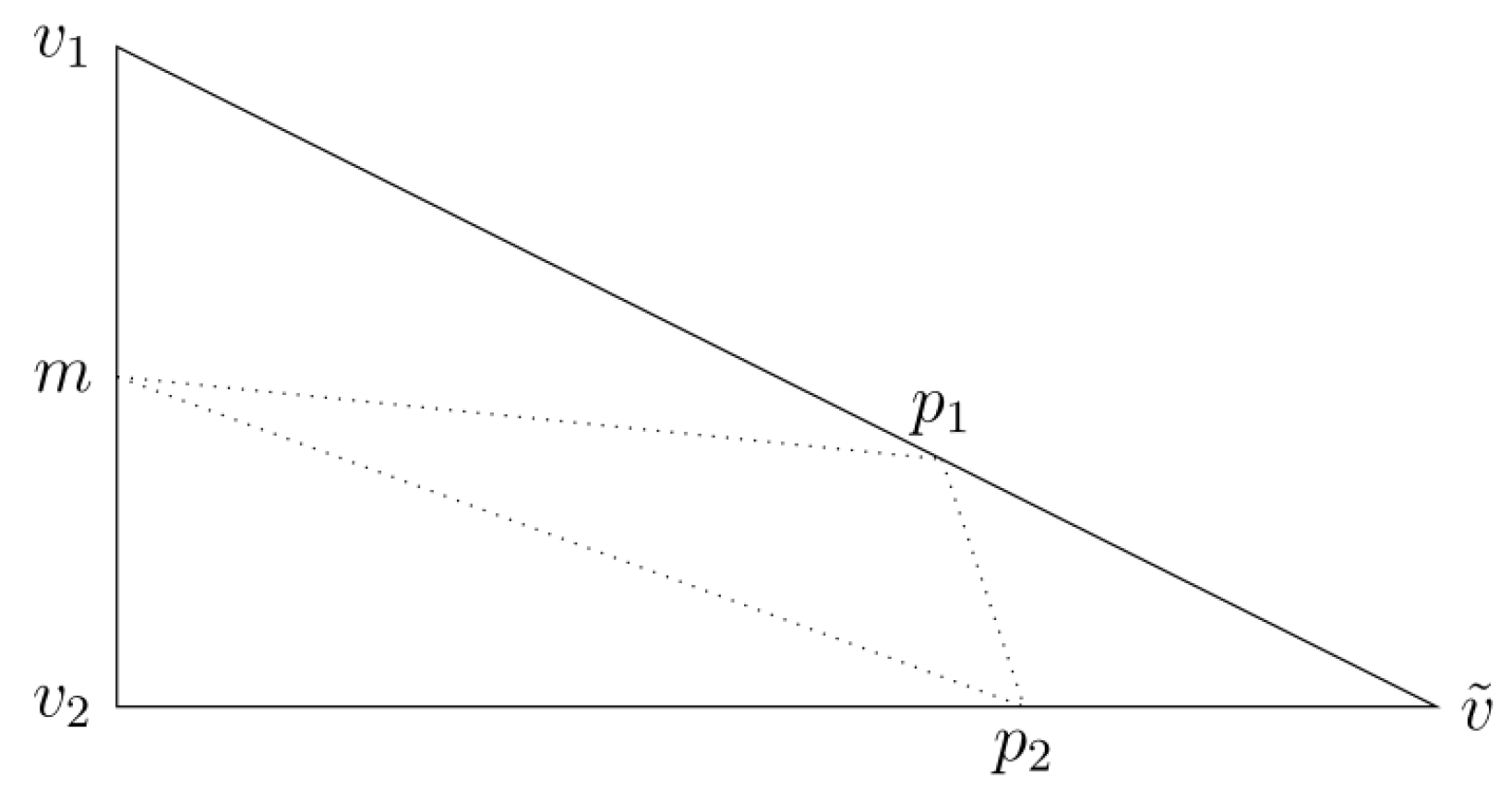
Figure 2.
The triangulation .
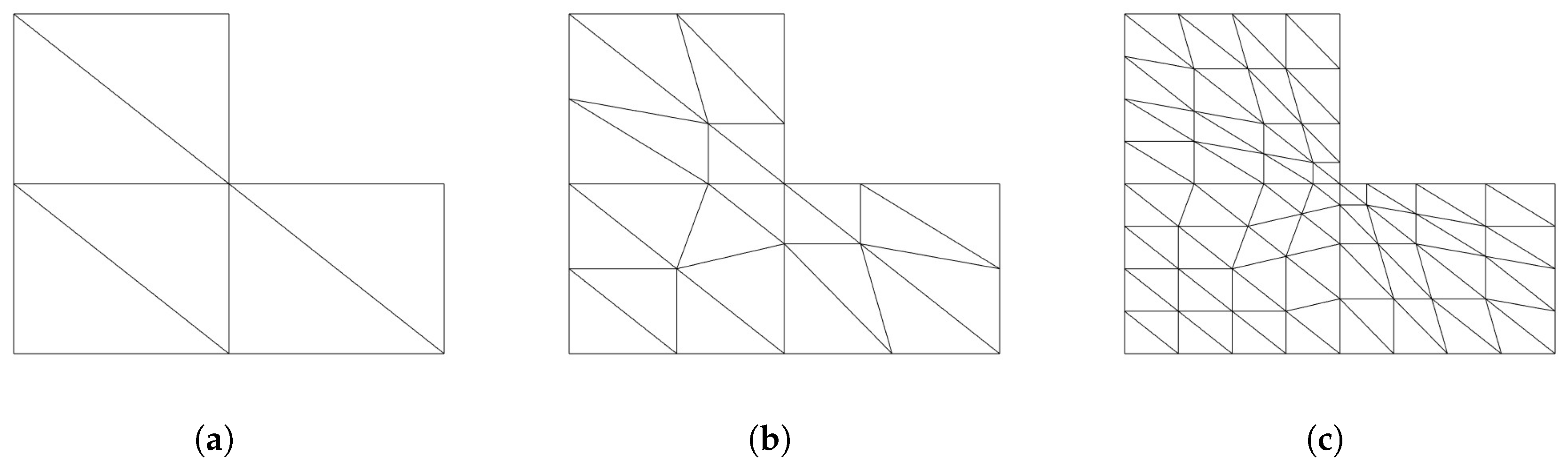

Table 1.
Results on the L-shaped domain and the exact solution given by (4.1).
| order | order | |||
|---|---|---|---|---|
| 1/2 | 3.94E-03 | 1.2896 | 4.05E-03 | 1.0477 |
| 1/4 | 1.82E-03 | 1.1099 | 2.17E-03 | 0.9038 |
| 1/8 | 1.02E-03 | 0.8399 | 1.13E-03 | 0.9406 |
| 1/16 | 6.03E-04 | 0.7554 | 5.73E-04 | 0.9794 |
| 1/32 | 3.23E-04 | 0.9030 | 2.87E-04 | 0.9957 |
| 1/64 | 1.67E-04 | 0.9506 | 1.44E-04 | 0.9992 |
Table 2.
Results on the doubly connected domain and the right hand side given by (4.3).
| order | order | c | ||||
|---|---|---|---|---|---|---|
| 1/8 | 1.91E-02 | 0.58 | 7.93E-02 | 0.72 | -0.3062 | -0.3059 |
| 1/16 | 1.23E-02 | 0.64 | 4.17E-02 | 0.93 | -0.3224 | -0.3040 |
| 1/32 | 7.13E-03 | 0.79 | 2.04E-02 | 1.03 | -0.2984 | -0.3036 |
| 1/64 | 3.63E-03 | 0.98 | 9.66E-03 | 1.08 | -0.2913 | -0.3037 |
Disclaimer/Publisher’s Note: The statements, opinions and data contained in all publications are solely those of the individual author(s) and contributor(s) and not of MDPI and/or the editor(s). MDPI and/or the editor(s) disclaim responsibility for any injury to people or property resulting from any ideas, methods, instructions or products referred to in the content. |
© 2025 by the authors. Licensee MDPI, Basel, Switzerland. This article is an open access article distributed under the terms and conditions of the Creative Commons Attribution (CC BY) license (http://creativecommons.org/licenses/by/4.0/).
Copyright: This open access article is published under a Creative Commons CC BY 4.0 license, which permit the free download, distribution, and reuse, provided that the author and preprint are cited in any reuse.


