
Submitted:
12 March 2025
Posted:
14 March 2025
You are already at the latest version
Abstract
Aiming at the problem of blind reclosing in permanent fault in active distribution network, a non-fault identification method before three-phase reclosing based on parameter identification is proposed. After the three-phase trip of the fault line, the distributed generation (DG)is used to simultaneously apply three-phase symmetrical low-frequency voltage excitation to the isolated line. When there is no fault that is the transient fault arc is extinguished, the three-phase network is symmetrical and each phase equivalent circuit is consisted of its own loop resistance and inductance. But in the case of permanent fault, the three-phase is asymmetry and the fault phase equivalent circuits are related to the transition resistance and fault location etc., which cannot be characterized as the aforementioned linear relationship. Therefore, using the differences to identify the fault condition before reclosing. Based on the principle of parameter identification, the R-L network in the non-fault is used as the reference model. Using the voltage and current information on the line side during the excitation period, and the least squares algorithm is used to calculate the resistance and inductance parameters of each phase circuit. When the calculated values of the resistance and inductance are consistent with the corresponding actual values, it is determined that the arc is extinguished and there is no fault. Simulation was conducted using PSCAD in different situations, and the results showed that the proposed non-fault detection method can effectively identify the fault condition before reclosing, and it does not require additional disturbance source equipment, which is helpful for the application and practice of adaptive three-phase reclosing in distribution lines.
Keywords:
active distribution network
; distributed generation
; adaptive three-phase reclosure
; non-fault detection
; parameter identification
1. Introduction
With the rapid development of clean and renewable distributed generation (DG)[1,2], traditional passive distribution networks have become active networks, and this transformation not only improves the complexity and diversity of the distribution network [3], but also brings new challenges to the traditional protection and fault handling modes. Relevant statistics show that more than 80% of the faults occurring in distribution networks are transient faults [4], so the use of pre-accelerated reclosing can significantly shorten the outage time and further improve the reliability of power supply in distribution networks. The current main strategy for DG access is to increase the check no-voltage step, but since most of the existing distribution network lines are configured with circuit breakers only on the system side, the implementation of the check no-voltage usually requires the new energy downstream of the fault point to stop operation, and the reclosing on the permanent fault may cause a secondary impact on the system, further worsening the fault condition and aggravating the damage of the equipment [5].
In order to overcome this shortcoming of traditional auto-reclosure, scholars have proposed adaptive reclosing that identifies the nature of the fault before the circuit breaker recloses, so as to avoid reclosing on the faulty line [6]. At present, for the high-voltage transmission line adaptive reclosing technology has been carried out a lot of research [7,8,9], distribution lines in the voltage level and the structure is obviously different from the transmission line [10], resulting in the transmission line existing fault detection technology directly used in the distribution network effect is not ideal, therefore there is a need to study adaptive reclosing methods for distribution networks. Existing fault detection methods for distribution networks are divided into two main categories, one is the fault detection technique using the line's own electrical quantity [11], but it is susceptible to fault location, and transition resistance, and is difficult to measure when the electrical quantity decays too fast. The second category is mainly fault detection techniques using applied disturbance devices, which utility the response characteristics of the line to applied disturbances for phase-to-phase fault discrimination [12,13]. One of the methods in this category is based on the scheme of identifying the nature of faults by perturbation signals from traditional electrical equipment. [14] uses a DC source to cast a pre-charged additional capacitor to the fault line several times, and screens the fault circuit according to the attenuation characteristics of the capacitor current. In [15], the external disturbance is applied to three phase-to-phase circuits in turn. The fault circuit is identified by the significant difference between the disturbance current of the fault phase-to-phase circuit and the other two non-fault phase-to-phase circuits. The disturbance signal is further applied to the fault phase-to-phase circuit, and the fault type is identified by the difference between the two disturbance currents. The other is based on the high controllability of power electronic equipment to provide effective fault characteristics for fault screening. [16] adds the inverter power supply to the distribution transformer, and uses the relationship between the line wave impedance and frequency to identify the faulty line. [17] applies a voltage perturbation signal to the grid using the inverter power supply and estimates the resistance and inductance at the excitation end through parameter identification techniques, and compares the parameter values obtained from the estimation with the real values of the actual circuit. The estimated parameter values are compared with the real values of the actual circuit to discern the nature of the fault. The use of external perturbation fault detection scheme has become an effective way to solve the lack of available signals after the tripping of distribution lines, but requires additional configuration of the corresponding dedicated perturbation source. Along with a large number of distributed DGs accessing the distribution network, it has become possible to apply short-duration perturbation excitation using the additional control of the line-accessed DG own power electronics after the tripping of the system-side circuit breaker after a fault [18], which provides a new way of thinking to implement the injective fault detection scheme.
In recent years, the parameter identification principle has been extensively investigated in novel protection schemes for high-voltage transmission lines [19], transformer protection [20], and adaptive reclosing [21]. It has demonstrated advantages such as immunity to decaying DC components and reduced requirements for filtering devices, attracting significant attention from researchers. Based on the concept of parameter identification, this paper investigates a non-fault phase detection method for active distribution networks to achieve adaptive three-phase reclosing. After three-phase tripping of the faulted line outline breaker in the distribution network, the connected DG inverter is utilized to briefly inject three-phase symmetrical low-frequency voltage excitation signals into the de-energized line. Using the non-fault RL equivalent network as the parameter identification reference model, the discrimination of fault-free conditions is achieved by analyzing the deviations between the identified resistance, inductance values and their corresponding actual measured values. Extensive simulation studies have verified the validity and effectiveness of the proposed method.
2. Fault Characterization
2.1. Fault Detection Scheme Using DG Injection
Taking Figure 1 as an example, this paper illustrates the non-fault detection scheme based on DG injection for distribution lines before three-phase reclosing [22]. After the three-phase tripping of the circuit breaker on power supply side due to a fault occurs in a distribution line, the residual electrical quantities are released after a fixed delay to avoid their impact on subsequent fault state detection results. At the same time, using the flexible and controllable characteristics of the DG inverter, the three-phase symmetrical voltage excitation is applied to the line to be detected by the DG for a short time. Using the difference in the characteristics of the circuit response at the point of common coupling (PCC) of the detected line during the excitation period, the fault state is further identified based on the results of model parameter identification. If it is judged to be a non-fault state, the three-phase reclosing on the line side avoids the risk of blind reclosing failure.
Among them, the amplitude and frequency of the three-phase voltage excitation applied by DG are the key parameters of the injection fault detection scheme. Considering that the measurement accuracy of 10kV voltage transformer is not less than 5% of the rated voltage, that is, the amplitude of the injected voltage should be satisfied the relation, i.e.. At the same time, reference [23] stipulates that the permissible deviation of supply voltage of 10kV and below is ±7% of the rated voltage. The range for the amplitude of injected voltage excitation is limited by the relation, i.e..
At the same time, the frequency of DG injection voltage excitation should be under the premise of satisfying the inverter own working parameters and performance constraints, so that the permanent fault and the instantaneous fault characteristics of arc extinction are significantly different to improve the sensitivity of fault detection [24]. In this paper, the idea of parameter identification is used to identify the time domain method of fault identification [25]. It involves the calculation of differential substitution derivative of sampling value, which requires high sampling frequency. Usually, the calculation step size is. In order to reduce the influence of line capacitance and communication and detection results, the frequency of the excitation signal should be selected as low as possible, usually its frequency is limited by[17].
2.2. Fault Modelling
Taking an AB phase-to-phase fault on the line as an example, this paper conducts a comparative analysis of the equivalent networks under transient fault (non-fault) conditions and permanent fault conditions
2.2.1. Transient Fault (i.e., Non-Fault)
When the distribution line is non-fault or the transient fault has been cleared, its equivalent network is shown in Figure 2. Where, are the voltages at the PCC, and is the current in each phase, is the self-resistance of each phase line, is the self-inductance of each phase line, is the equivalent inductance of the distribution transformer, and N is the virtual neutral point.
Obviously, when the three-phase symmetrical low-frequency voltage excitation is applied simultaneously by the DG, if the line is in a non-fault state at this time, the three-phase is symmetrical. The three-phase equivalent network shown in Figure 2 is equivalent to the single-phase equivalent network shown in Figure 3 for analysis.
The equivalent network equations shown in Figure 3 can be obtained as shown in equation (1):
From equation (1), the excitation voltage of any phase is consisted by a linear relationship between and of each phase circuit of the line.
2.2.2. Permanent Fault
Similarly, if the phase-to-phase fault still exists when voltage excitation is applied, the line equivalent network is shown in Figure 4. In which, is the fault transition resistance, m is the distance from the fault point to the first end of the line as a proportion of the total length of the line. is the equivalent impedance from the point of failure to the end of the line.
The equivalent network equation shown in Figure 4 can be obtained as shown in equation (2):
where ,
Obviously, the excitation voltage for any of the faulted phases is related to the fault point location m, the transition resistance and the excitation voltageof the other phase, and it cannot be characterized as a linear relationship as shown in equation(1). For a two-phase ground fault, a similar relationship exists as in equation (2).
In addition, since three-phase fault is symmetrical fault, it can also be analyzed as a single-phase equivalent circuit, and the relationship is shown in equation (3).
From equation (3), it can be seen that the excitation voltage of each phase generated by the DG is related to the resistance and inductanceof the line itself from the fault point to the DG access point, i.e., the fault location m is related to the resistance parameter and the inductance parameter in the model, which are significantly different from those in the case of non-fault condition.
From equation (1) to equation (3), it can be seen that there is a significant difference between the non-fault equivalent network and the permanent fault equivalent network, so the difference can be utilized for the screening of the fault state of the three-phase circuit. Based on the principle of model parameter identification, the R-L equivalent network in non-fault state is used as the reference model, and the voltage and current at the PCC during the excitation period are collected to calculate the equivalent resistance and inductance of the line to be detected, and the fault state is identified based on the difference between the recognized values of resistance and inductance and the corresponding actual values.
3. Non-Fault Detection Principle and Criterion Based on R-L Parameter Identification
3.1. Fundamentals
After the exit circuit breaker trips after a fault in the distribution line, the DG simultaneously produces a low-frequency voltage excitation to the three phases of the detection line after the fault has disappeared if the fault has disappeared before applying the excitation, at this time, the excitation voltage at the PCC has a linear relationship with the response current and the response current derivative, and the corresponding expression is:
According to the sampling value of excitation voltage and response current at different times, the matrix expression is obtained as follows:
In this paper, the R-L non-fault equivalent network shown in Figure 3 is used as a calculation model, for the non-fault line,is the line resistance value , while for the faulty line, the existence of the transition resistance leads to the change of the equivalent circuit, at this time, ,is related to the fault location and transition resistance.
In order to calculate and , the collected excitation voltages and currents are fit to linear equations using the least squares method [25], thus obtaining two linear equations, and , for solving coefficients. For the presence of faults, there is a significant difference between the identified resistance value of line parameters and the corresponding true resistance and there is a significant difference between the identified inductance value and the corresponding true inductance value. And when the parameter identification results are highly consistent with the corresponding true values, that isand. And it indicates that the actual model is consistent with the reference non-fault model, i.e., the line is in non-fault state.
Construct the objective function as follows
Where is the excitation voltage at the kth sampling point, is the current at the kth sampling point, and N is the number of sampling points.
Taking the partial derivatives for , and their extremes, respectively
Using equation (7), the identification values of the equivalent resistance and equivalent inductance of the line can be obtained.
3.2. Non-Fault Identification Criteria
The fitting evaluation coefficients and obtained through linear fitting using the least squares method can be used to identify the nature of the fault. For transient fault, the calculatedandare equal to the actual valuesand. But for permanent fault, the calculated values of and are significantly different from the actual values of and . Aiming at the difference between and obtained by parameter identification and the actual values and ,the non-fault identification criterion is proposed as shown in equation ( 8 ) :
Where,the identification deviation values of resistances and inductances are represented asand respectively .
And more, n is the length of the sequence of calculation results, is the least squares calculation of resistance sequence, is the least squares calculation of inductance sequence, are the margin factors. Due to the influence of model error and algorithm calculation error, the criterion needs to reserve a certain margin. The coefficientsare set from 0.1 to 0.2, which can meet the requirements of fault nature discrimination. When the two conditions of equation (8) are met, it can be judged as a non-fault state (i.e. a instantaneous fault with arc extinction). Otherwise, it is judged as a persistent state fault,i.e., a permanent fault.
3.3. Realizing Scheme
The implementation of the active distribution network phase-to-phase fault state identification proposed in this paper is shown in Figure 5.
Step 1:In order to avoid the influence of residual electrical quantities in the fault line on the discrimination results after the three-phase trip of the distribution line fault, a low-frequency voltage excitation is applied to the three phases of the tested line by DG after the breaker trips with a 50ms-100ms delay.
Step 2:Collect voltageand currentdata at PCC, then sequentially solve the three-phase resistance and inductance parameter identification values using equation (7).
Step 3:If the criterion shown in equation (8) is satisfied, it is determined as a non-fault state (indicating the arc extinction state of transient fault), and the circuit breaker will issue a reclosing command. If the criterion remains unsatisfied until the maximum discrimination time is reached, it is determined that the inter-phase loop still contains a fault (i.e. considered as permanent fault), the reclosing operation will be blocked. When the maximum allowed discrimination time is not yet reached, the process returns to step (2) for iterative determination.
4. Simulation Verification
4.1. Simulation Model
4.2. Simulation Calculations
4.2.1. Identification Criterion Principles Verification
It is assumed that the AB phase-to-phase fault with a transition resistance of 10Ωoccurs at the midpoint of the line L5, the fault occurs in 0.3s, the three-phase tripping of the outlet circuit breaker in 0.32s, and the voltage of 20V/10Hz is applied to the three-phase of the line L5 to be detected at the same time by the DG in 0.6s. The voltage excitation of 500V/10Hz can be obtained through the step-up transformer. The transient fault lasts for 0.7s, and the permanent fault lasts until the end of the simulation. The sampling frequency is 10 kHz, and the length of the calculation data window is 20ms, that is, 200 sampling data is used to calculate a set of resistance and inductance.
The actual values of resistance and inductance of each phase of the corresponding non-fault circuit are calculated as follows
Where, is the positive sequence resistance of the line, is the positive sequence inductance of the line, is the nominal value of the distribution transformer, is the rated voltage of the primary side of the distribution transformer, is the rated capacity of the distribution transformer, andis the angular frequency at the industrial frequency.
After calculating the actual values of resistance and inductance, the threshold value of the criterion can be further calculated. The reliability coefficients and are 0.2. According to equation (8), the action threshold corresponding to the criterion is
When both the identified resistance and inductance values satisfy the relationship defined in equation (10), it is reliably judged as non-fault condition. When at least one parameter (resistance or inductance) fails to satisfy the equation (10), it indicates the existence of an permanent inter-phase fault on the line.
To demonstrate the effectiveness of the proposed discrimination method, Figure 7 and Figure 8 present the identification results of the three-phase resistance and inductance parameters for line L5 under AB phase-to-phase permanent fault and transient fault conditions.
As can be seen from the results shown in Figure 7, when a permanent fault occurs, the actual fault model is inconsistent with the recognition model, and the corresponding resistance and inductance recognition values are significantly different from the actual resistance and inductance parameters, of which the three-phase resistance parameter recognition deviations are =1.654Ω、=0.400Ωand =0.010Ω respectively. Moreover, the three-phase inductance parameter recognition deviations are =13.7mH、=23.4mH and =0.010mH respectively, which means that the relationship between the three-phase resistance and inductance identification results and the corresponding real values has at least one item that does not satisfy the relationship shown in equation (10), which indicates that the fault is on the line L5 and the arc has not been extinguished.
Figure 8 shows the the results of a transient fault. Before the fault disappears at 1.0s, the actual fault model and the identification model are inconsistent. Significant discrepancies exist between the identified resistance, inductance values and the corresponding actual values, and the exhibiting characteristics is similar to those of permanent faults described aforementioned.
After the fault disappears at 1.0s, The actual fault model aligns with the identification model. The identified resistance and inductance parameters match the actual parameters, with maximum deviations of =0.013 Ω for resistance andfor inductance. During this phase, the relationship between the three-phase resistance or inductance identification results of line L5 and their true values consistently satisfies the relationship defined in equation (10). Thus, line L5 is reliably judged to be in a non-fault state.
4.2.2. Performance Analysis Under Different Fault Conditions
In order to verify the applicability of the proposed method in the first section and the end of the line, this paper designs the following 4 scenarios according to different transition resistances. The calculation results of AB phase-to-phase faults under different conditions of line L5 are shown in Figure 9 and Figure 10.
- Scenario 1: Transient fault occurs with 1 Ω transition resistance.
- Scenario 2: Permanent fault occurs with 5 Ω transition resistance.
- Scenario 3: Permanent fault occurs with 10 Ω transition resistance.
- Scenario 4: Permanent fault occurs with 20 Ω transition resistance.
Next, simulation calculations are carried out separately for the four fault scenarios mentioned above at the beginning and end of the line. The result of AB phase-to-phase short circuit at the head of the line (m=0.1) and at the end of the line (m=0.9) are shown in Figure 10 respectively.
The results of an AB phase-to-phase short circuit at the beginning of the line are shown in Figure 9.
In scenario 1,both the resistance and inductance deviations are smaller than the threshold values, so the line is judged as no fault. And in scenarios 2–4,even with a transition resistance of 20Ω (the transition resistance for phase-to-phase faults generally does not exceed 20Ω), the deviations of the three-phase resistance identification values (=1.36Ω, =0.328Ω) differ from the actual resistance value=0.25Ω. Additionally, the identified inductance value =17.09mH significantly deviates from the actual inductance value =12.69mH. These discrepancies violate the relationship defined in Equation (10), failing to meet the non-fault criteria, and are thus identified as permanent faults.
The results of an AB phase-to-phase short circuit at the end of the line are shown in Figure 10. In scenario 1, the differences between the calculated values and actual values of both resistance and inductance satisfy equation (10), thus it judges as a non-fault condition. In scenarios 2-3, even with a transition resistance of 20Ω (the transition resistance for phase-to-phase faults generally does not exceed 20Ω), there remains significant discrepancy between the calculated resistance values (=0.961Ω and =0.53Ω) and the actual resistance value (=0.25Ω). In these cases, at least one parameter (either the actual resistance or actual inductance) shows significant deviation, failing to satisfy the non-fault criteria. Therefore, the criteria proposed in this paper can reliably identify inter-phase permanent faults
4.2.3. Comparison with Other Methods
To validate the superiority of the proposed method, voltage deviation analysis is designed based on the aforementioned four scenarios. During non-fault disturbance conditions, ignoring the line impedance and transformer impedance, the voltage difference between the PCC voltage () and the injection source voltage referred to the high-voltage side ( ) is zero. When a phase-to-phase fault occurs, an inter-phase loop forms with fault current circulation, causing elevation of . In this case, significant deviation emerges in the voltage difference between and . Considering the transformer impedance voltage drop, system modeling errors, and voltage transformer measurement accuracy, the discrimination criterion can be established as follows
In this paper, the transformer impedance voltage drop is set to 1%~2% of the source voltage. Additionally, the discrimination criterion requires a safety margin, where is ranged from 1 to 3 meets the requirements for fault type identification. Therefore, .
When the line voltage deviation satisfies equation (11), the condition is determined as non-fault. Conversely, failure to meet equation (11) indicates the occurrence of a phase-to-phase fault on the line.
Figure 11 shows the voltage deviations during an AB phase-to-phase fault at the sending terminal of the line. In Scenario 1, both voltage deviations of phases A and B , satisfy the criterion shown in equation (11), leading to a non-fault determination. In scenarios 2-3, the voltage deviations of faulted phases AB exceed the threshold, resulting in permanent fault identification.
To compare the sensitivity of both methods, the sensitivity coefficients for the aforementioned criteria are calculated using equation (12), where, , and all adopt the maximum values in each phase. The calculation results for the four predefined scenarios are summarized in Table 2.
The sensitivity comparison of both methods for an AB phase-to-phase fault at the sending terminal of the line is presented in Table 2. Although the inductance sensitivity drops below 0.5 after fault occurrence, the resistance sensitivity consistently remains above 0.5. The proposed method only requires either resistance or inductance sensitivity to meet the 0.5 threshold for reliable fault discrimination. Voltage sensitivity remains below 0.5 across all test scenarios in this study, confirming the superior sensitivity of the proposed method.
Furthermore, to validate the adaptability of the proposed scheme, extensive simulation studies verify that the method reliably discriminates pre-reclosing fault conditions: it enables successful reclosing when non-fault status is identified, and securely blocks reclosing for permanent faults. This effectively mitigates the risk of secondary impacts caused by blind reclosing onto permanent faults.
5. Conclusions
This paper proposes a three-phase reclosing fault condition detection method for distribution networks integrated with DG. The method leverages model parameter identification under transient disturbance excitation from DG connected to the target line. Key conclusions are:
After three-phase tripping due to an inter-phase fault, in the case of non-fault condition (i.e. a transient fault with arc extinction), the equivalent network consists of linear combinations of equivalent resistance and inductance in each phase circuit. Permanent fault condition: The fault equivalent network depends on transition resistance and fault location, which cannot be represented as linear relationships.
Moreover, adopting the principle of parameter identification, the non-fault R-L equivalent network is used as the identification model. The resistance and inductance parameters are identified using the response voltage and current values during the DG disturbance on the line side, and a non-fault discrimination scheme before three-phase reclosing is constructed by using the difference between the identified values of resistance and inductance and the actual values.
Furthermore, the proposed method directly utilizes time-domain voltage and current signals without high filtering requirement, and is independent of additional disturbance injection equipment. It enables rapid and reliable non-fault discrimination in various fault scenarios, and the simulation results verify the correctness and effectiveness of the proposed approach.
Author Contributions
Conceptualization, Z.S. and S.A; methodology, W.S. and D.L.; validation, X.S., S.Z.; formal analysis, S.A., D.L And W.S.; investigation, S.Z. and W.S.; resources, S.A.; writing—original draft preparation, Z.S. and X.S; writing—review and editing, S.Z. and W.S.; visualization, S.Z. All authors have read and agreed to the published version of the manuscript.
Funding
This research was funded by the Technology Project supported by Inner Mongolia Electric Power (Group) Co., Ltd, grant number NJ-GKCG-2024-ZNPWB-0401-0028.
Conflicts of Interest
The authors declare that they have no conflicts of interest.
References
- Si R, Yan X, Liu W, Zhang P, Wang M, Li F, Yang J, Su X. Hybrid optimization-based sequential placement of DES in unbalanced active distribution networks considering multi-scenario operation. Energies. 2025; 18(3):474. [CrossRef]
- Ma X, Zhen W, Ren H, Zhang G, Zhang K, Dong H. A method for fault localization in distribution networks with high proportions of distributed generation based on graph convolutional networks. Energies. 2024; 17(22):5758.
- Ayanlade, Samson Oladayo and Funso Kehinde Ariyo. Optimal Allocation of photovoltaic distributed geberation in radial distribution networks. Sustainability, 2023, Volume 15, no.18, pp. 13933-13956.
- W.L.Gao, M.D.Xi and H.Wang. New method of small current grounding line selection based on feature fusion and extreme learning machine. Electronic Measurement Technology, 2023, Volume 46, no.13, pp. 176-184.
- J.W.Zhao, H.B.Zhang and Y.J.Hu. Adaptive distance protection for distributed generation distribution network with T-connected inverter interfaced distributed generation. Renewable Energy Resources, 2024, Volume 42, no.1, pp. 64-70.
- W.Q.Sao, Y.Liu and Z.H.Zhang. Non-Fault detection for three-phase reclosing in transmission lines based on calculated differential-currents. Power System and Clean Energy, 2017, Volume 33, no.1, pp. 18-23.
- H.Cao, Q.Xia and B.Yu .Intelligent reclosing strategy for near area AC transmission lines connected with UHVDC. Power System Protection and Control,2022, Volume 50, no.3, pp. 156-163.
- J.Shen, Z.S,Shu and J. Chen. Application of adaptive auto- reclosure in power system. Automation of Electric Power Systems, 2018, Volume 42, no.6, pp. 152-156.
- W.A. Khan, BI Tianshu and Jia Ke. A review of single phase adaptive auto-reclosing schemes for EHV transmission lines. Protection and Control of Modern Power Systems, 2019, Volume 4, no.3, pp. 205-214. [CrossRef]
- C.L. Li, C. Ma and C.Y. Wang .Study on relay protection of distribution network containing distributed generation based on adaptive algorithm. Renewable Energy Resources,2015, Volume 33, no.9, pp. 1329-1339.
- Z.H Zhang, H. Qiao and W.Q. Shao. Non-fault detection in phase-to-phase faults before reclosing in distribution network. Grid Analysis & Study,2018, Volume 46, no.2, pp. 66-71.
- H.Y. Liao,X.N. Kang and Y.L. Yuan. Adaptive three-phase reclosing device of distribution network based on injected signals. Power System Technology,2021, Volume 45, no.7, pp. 2623-2630.
- M.M. Song, J. Liu and Z.H. Zhang. Power quality analysis based on power consumption information acquisition data. Distribution &Utilization, 2020, Volume 37, no.10, pp. 51-57.
- W.Q.Shao, Y.X.Liu and X. Guan. An active detection scheme for permanent fault identification before phase-to-phase reclosing in a distribution network. Power System Protection and Control,2021, Volume 49, no.14, pp. 96-103.
- W.Q.Shao, Y.X.He and X.Guan. Identification method for an interphase permanent fault in a distribution network using waveform characteristics of multiple disturbance currents. Power System Protection and Control,2023, Volume 51, no.7, pp. 146-157.
- K.Zu, Y.T,Song and Y.G.Xu .An active adaptive reclosing scheme for distribution lines. Power System Technology,2017, Volume 41, no.3, pp. 993-999.
- J.Zhuo, W.Q,Shao and X.Guan. Permanent fault identification method of distribution network based on parameter identification. Distributed Energy,2022, Volume 7, no.1, pp. 37-45.
- Z.H Zhang, J.Liu and B.J Ren. Permanent fault identification for distribution network based on characteristic frequency signal injection using power electronic technology. Frontiers in Energy Research,2022, Volume 10, no. 9.
- J.L. Suonan, W.Q.Shao and G.B.Song. Study on Single-phase adaptive reclosure scheme based on parameter identification. Proceedings of the CSEE,2009, Volume 29, no.1, pp. 48-54.
- Z.B.Jiao, T.Ma and Y.J.Qu. A novel excitation inductance-based power transformer protection scheme. Proceedings of the CSEE, 2014, Volume 34, no.10, pp. 1658-1666.
- Z.H.Huang, J.Y. Zou and Q.T Zou .Research on controlled reclosing for solidly earthed neutral systems. Proceedings of the CSEE,2016, Volume 36, no.17, pp. 4753-4762.
- H.D. Chen F.Meng and L.Zhao. Fault identification technology for distribution line based on distributed generation injection signal. High Voltage Apparatus,2022. vol. 58, no.12, pp. 123-129+146. [CrossRef]
- GB/T 12325-2008 Quality of electric energy supply--Admissible deviation of supply voltage[S].
- R.D Xu, Z.X.Chang and G.B.Song . Grounding fault identification method for DC distribution network based on detection signal injection. Power System Technology, 2021 Volume 45, no.11, pp. 4269-4277.
- J.Y.Lin, R.chen, Y.L.LI. Fault Location Method for Distribution Network Based on Parameter Identification. Southern Power System Technology, 2019, Volume13, no.3, pp.80-87.
Figure 1.
Fault detection system based on injection by DG in active distribution network.
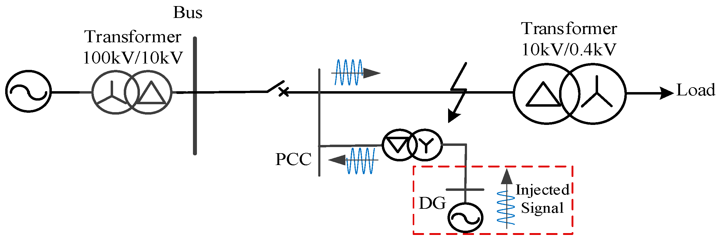
Figure 2.
Non-free equivalent network of distribution network
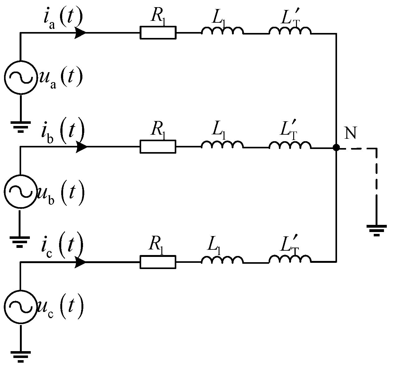
Figure 3.
Non-fault equivalent network diagram
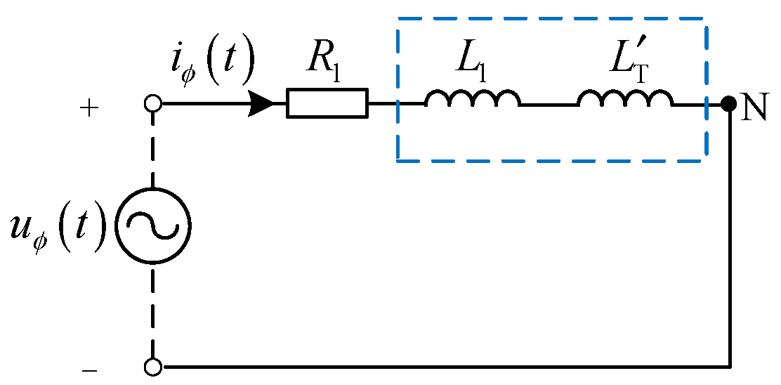
Figure 4.
Distribution line AB permanent fault equivalent network
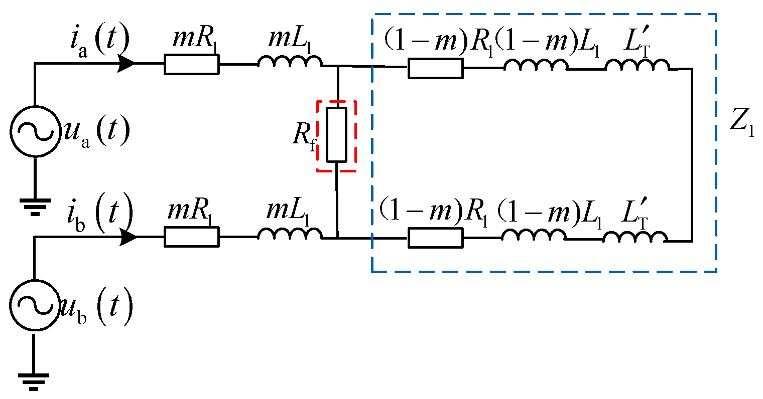
Figure 5.
Realizing scheme.
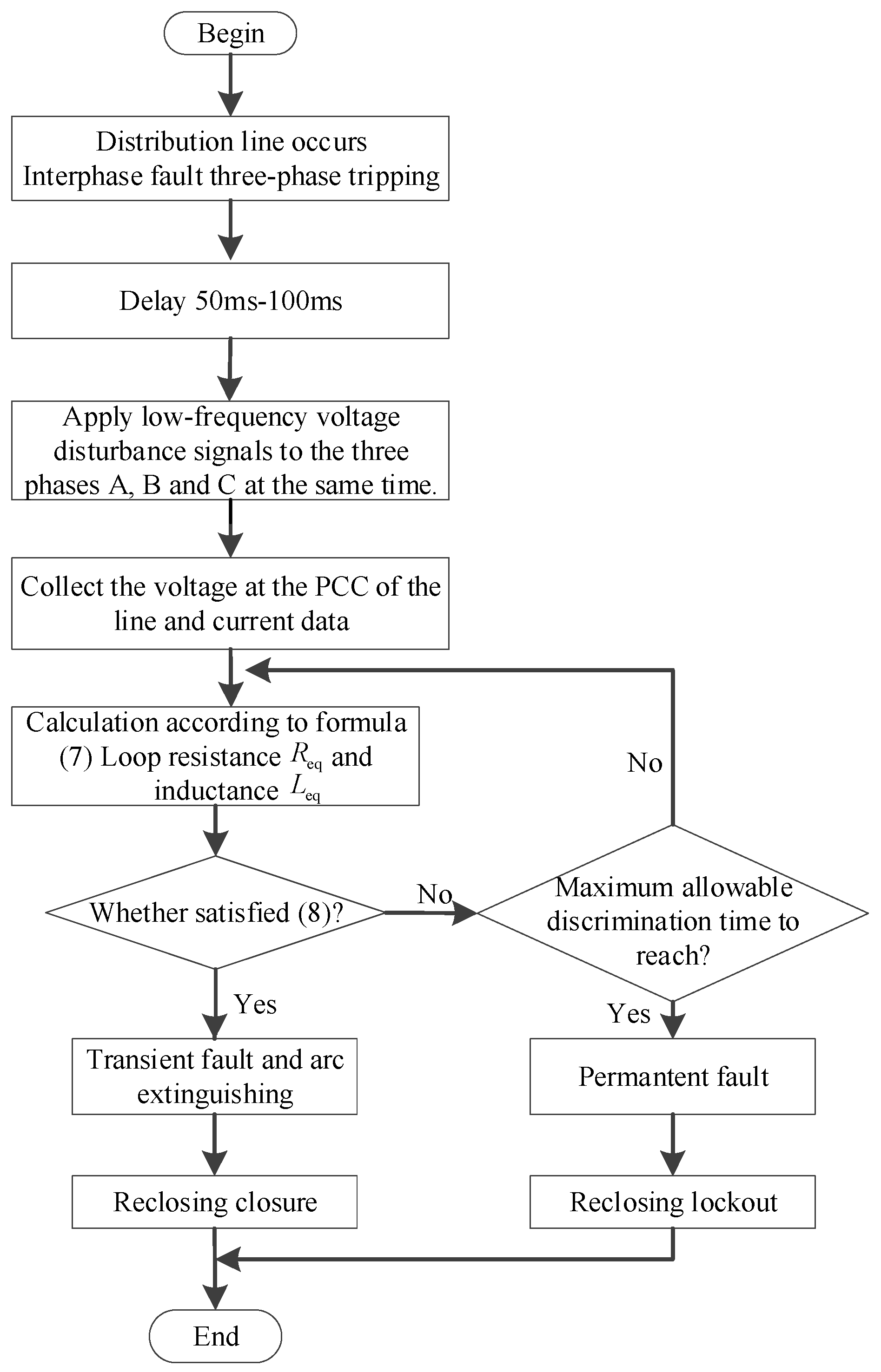
Figure 6.
10 kV distribution network model.
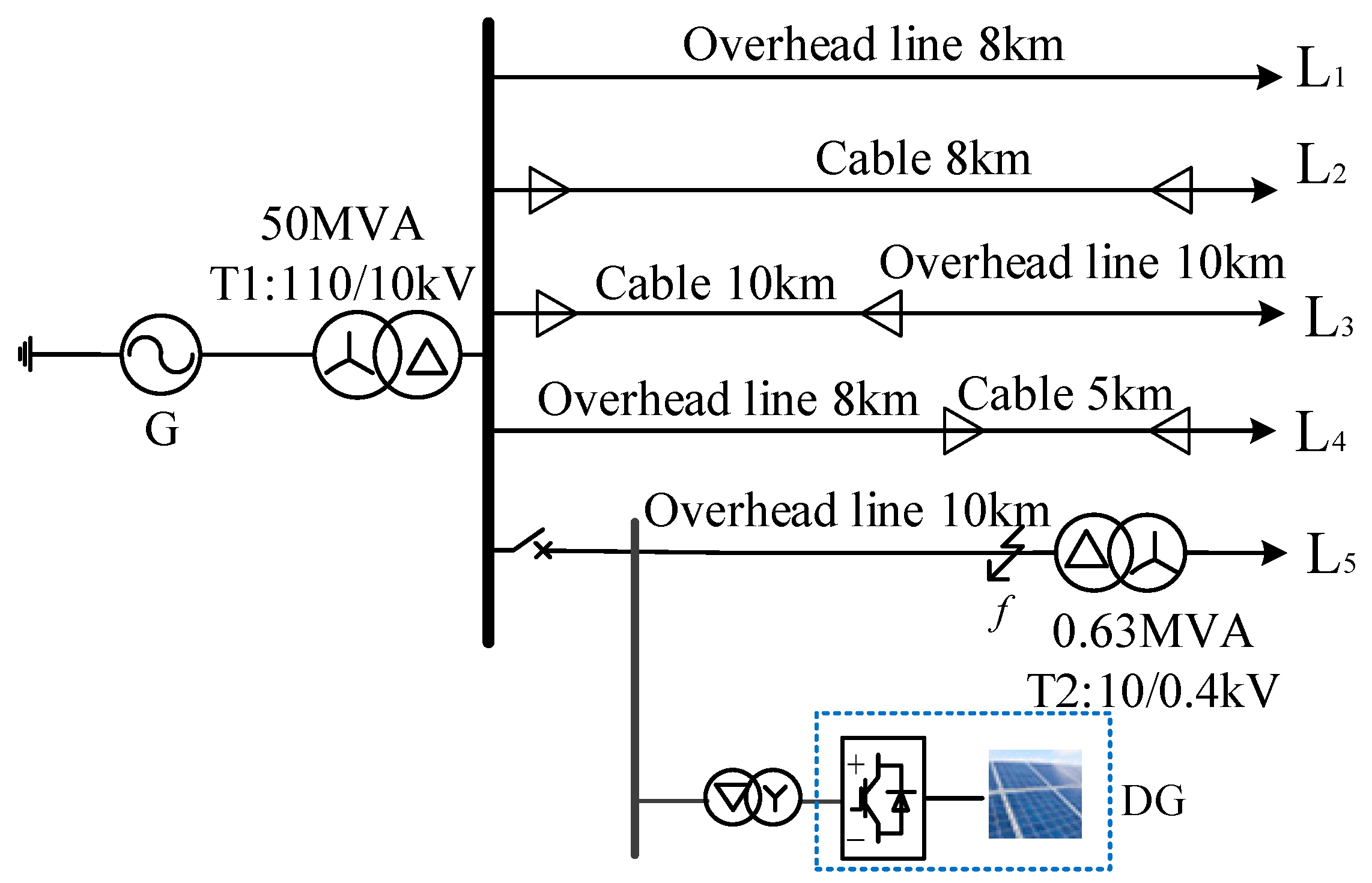
Figure 7.
Results of permanent fault.
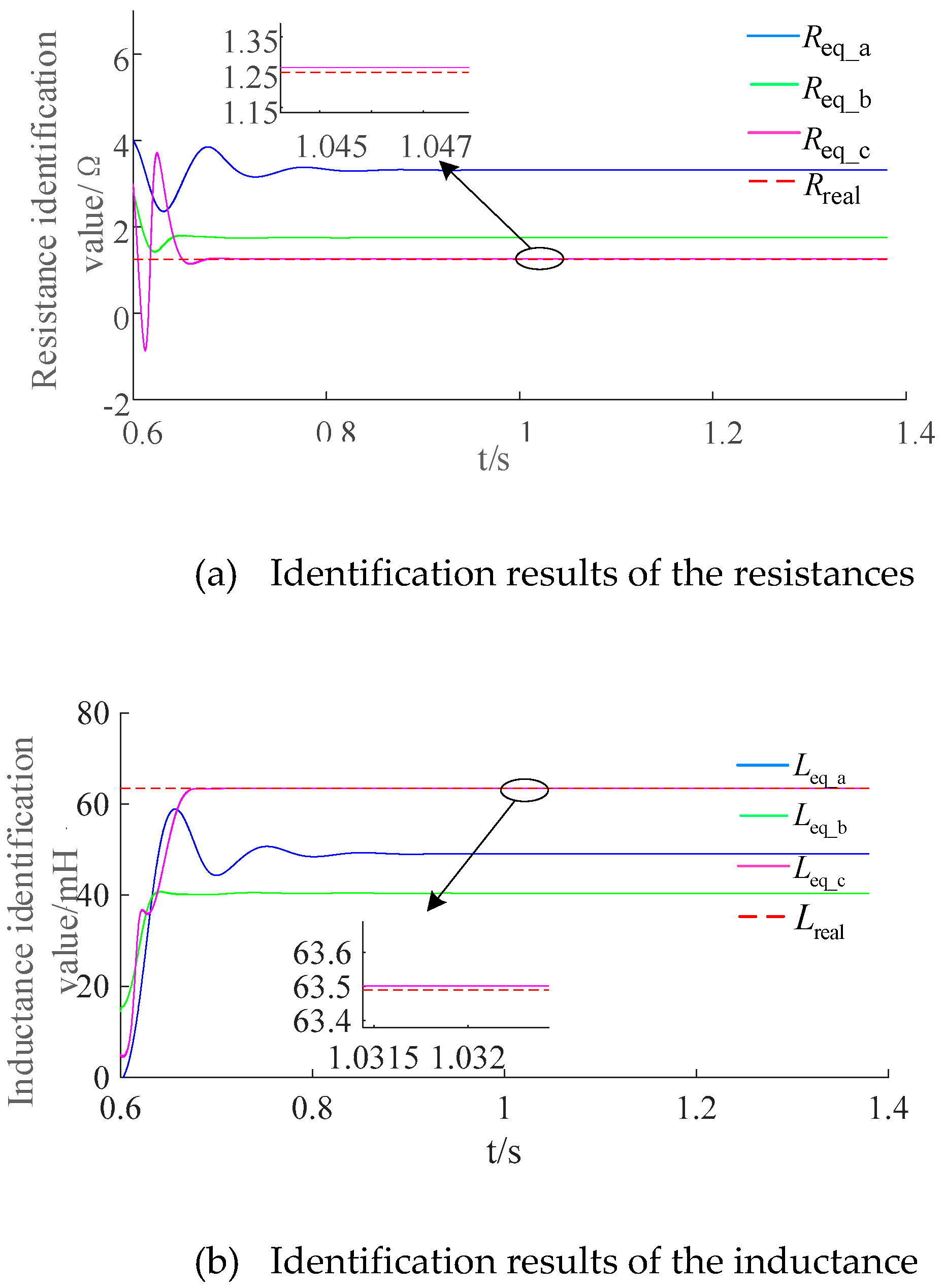
Figure 8.
Results of transient fault.
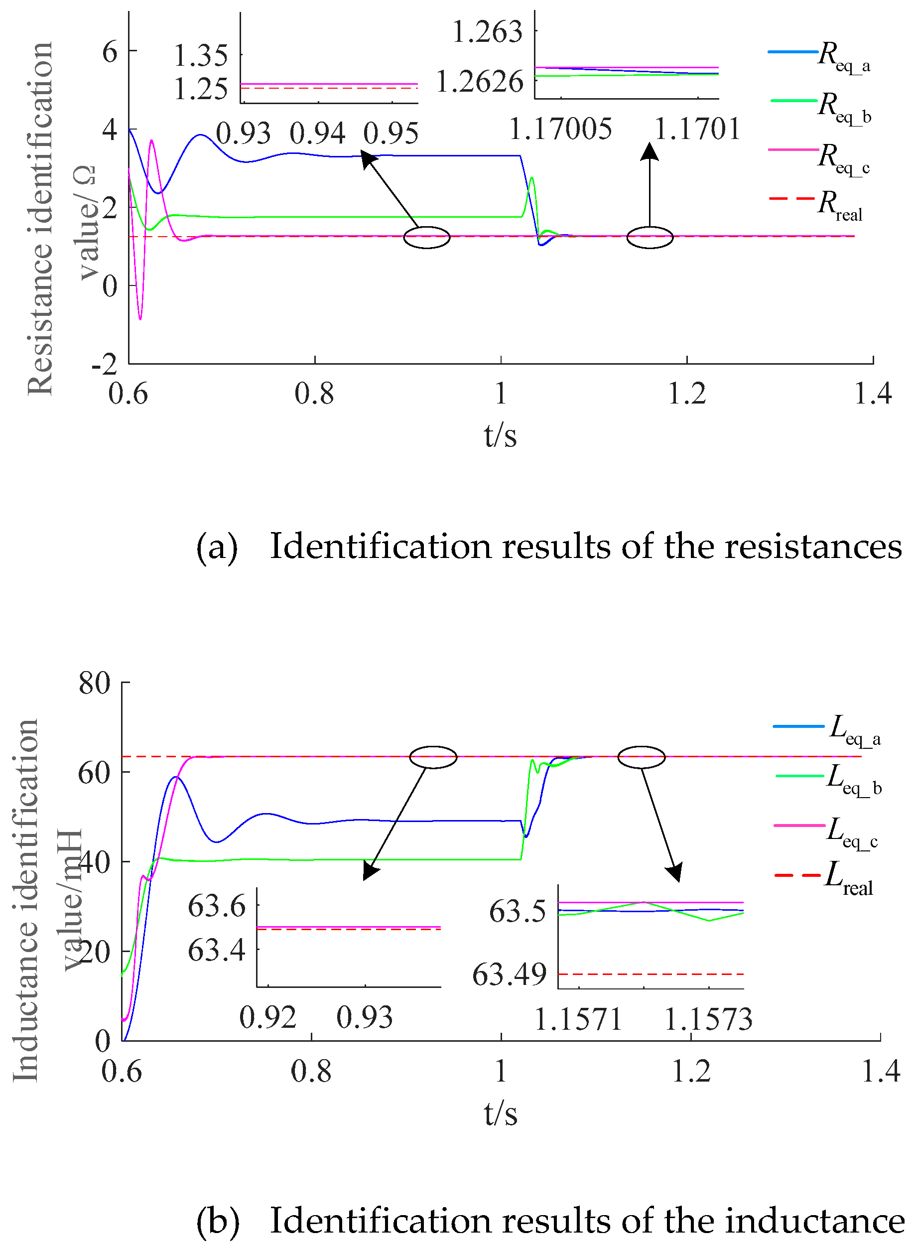
Figure 9.
Results of the faults occurring at the beginning of the line (m=0.1).
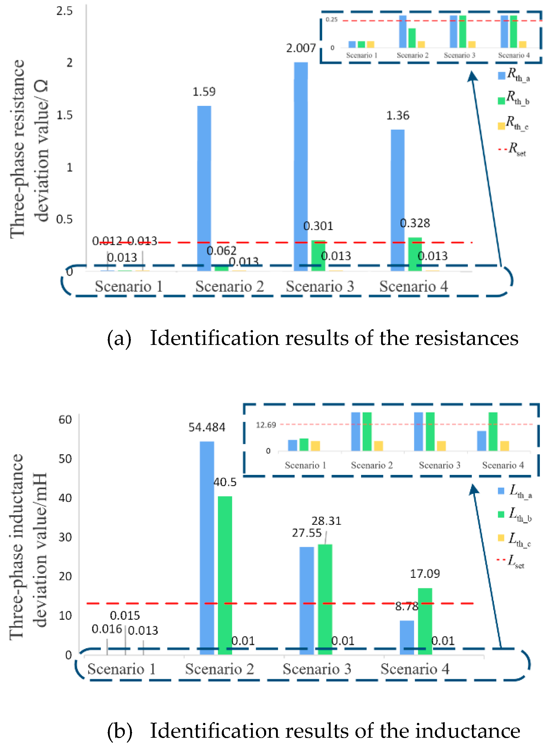
Figure 10.
Results of the faults occurring at the end of the line (m=0.9).
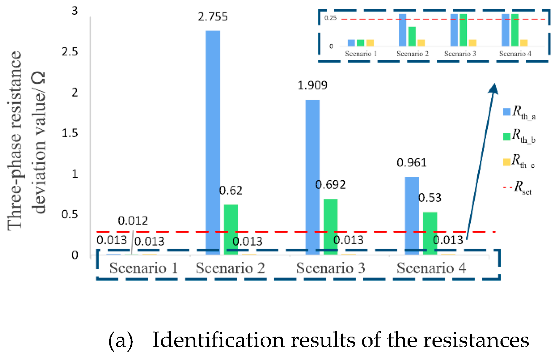
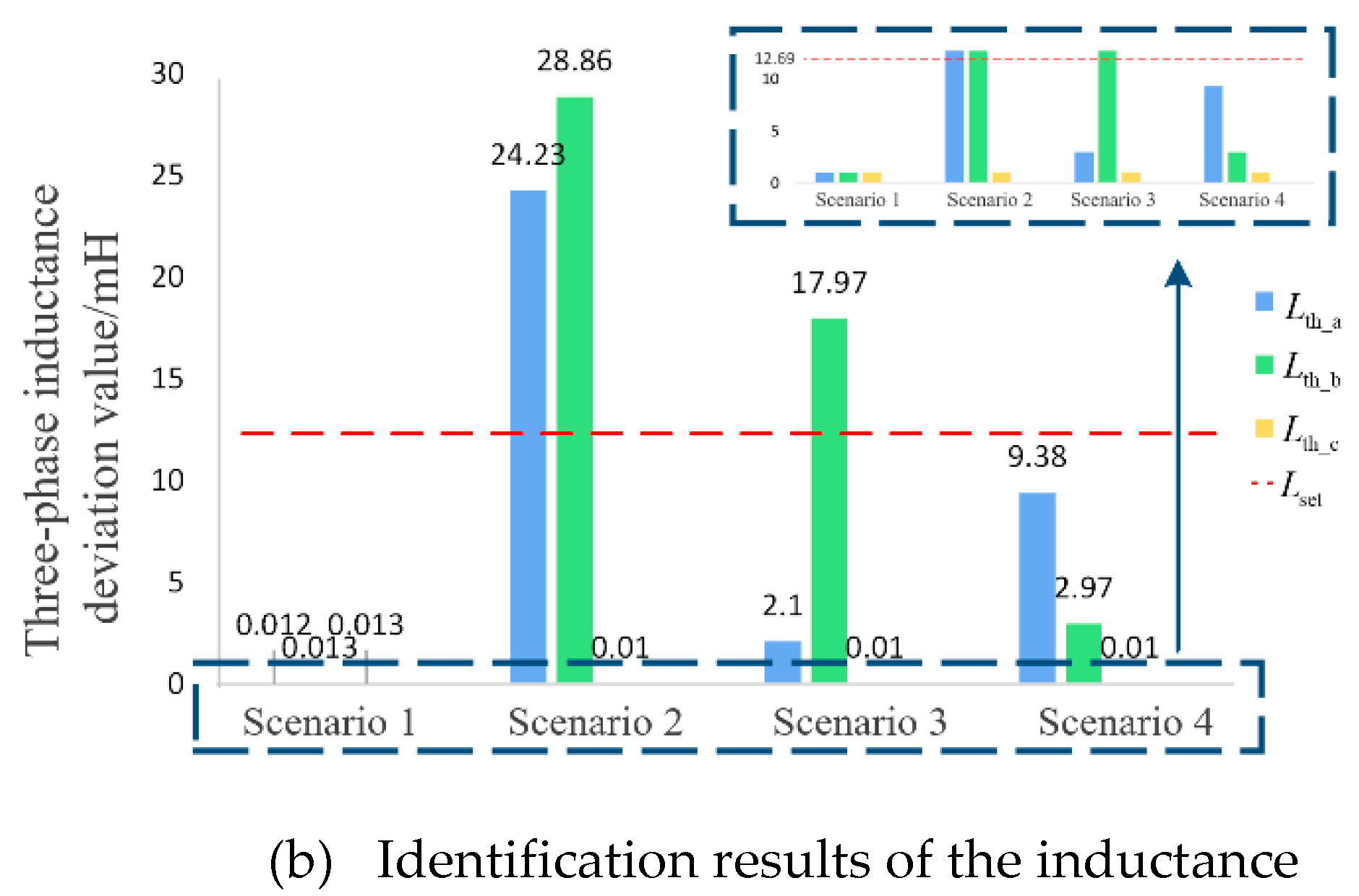
Figure 11.
Results of criterion using voltage deviation.
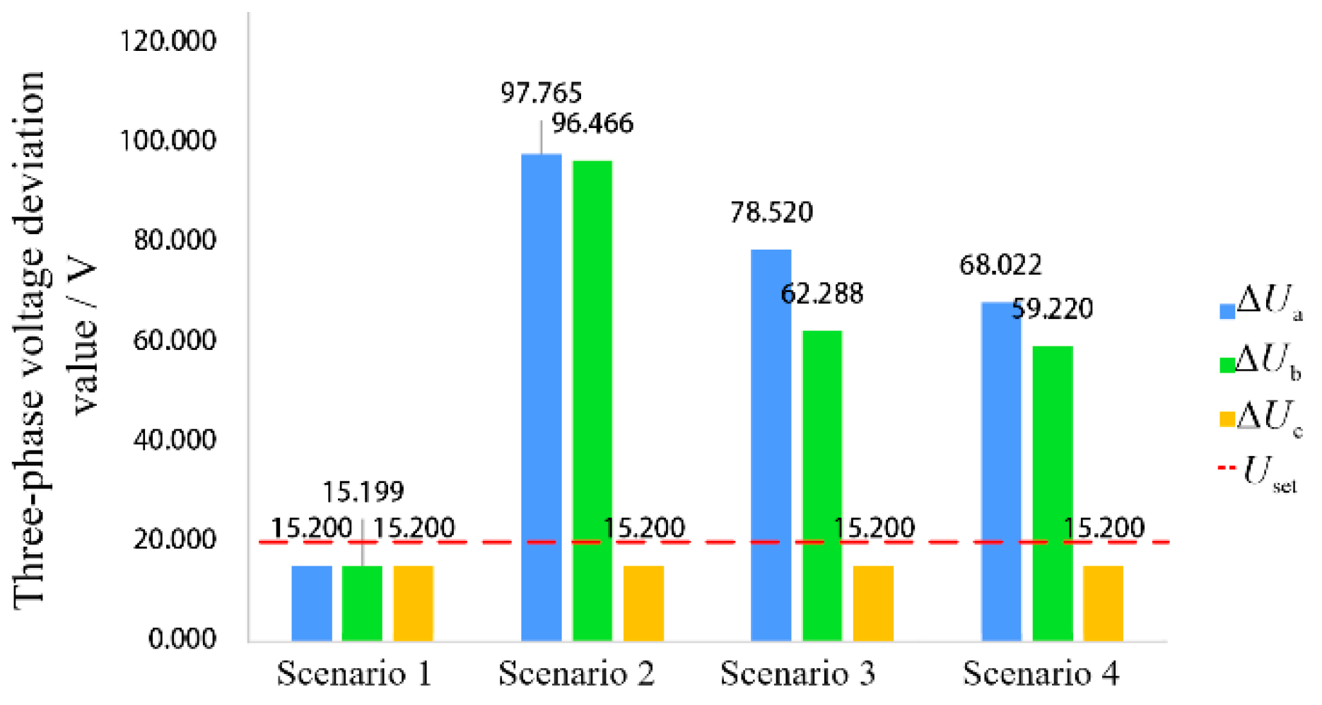

Table 1.
Distribution line parameters
| Line type | Phase sequence |
Resistance (Ω/km) |
Inductance (mH/km) |
|
|---|---|---|---|---|
| overhead line | positive sequence | 0.125 | 1.299 | 0.040 |
| zero sequence | 0.275 | 4.586 | 0.012 | |
| cable line | positive sequence | 0.270 | 0.254 | 0.339 |
| zero sequence | 2.700 | 1.019 | 0.280 |
Table 2.
Sensitivity coefficient
| Scenario | |||
| scenario 1 | 0.0072 | 0.0003 | 0.0310 |
| scenario 2 | 1.2720 | 0.6379 | 0.1930 |
| scenario 3 | 1.6056 | 0.4339 | 0.1252 |
| scenario 4 | 1.0880 | 0.26918 | 0.1184 |
Disclaimer/Publisher’s Note: The statements, opinions and data contained in all publications are solely those of the individual author(s) and contributor(s) and not of MDPI and/or the editor(s). MDPI and/or the editor(s) disclaim responsibility for any injury to people or property resulting from any ideas, methods, instructions or products referred to in the content. |
© 2025 by the authors. Licensee MDPI, Basel, Switzerland. This article is an open access article distributed under the terms and conditions of the Creative Commons Attribution (CC BY) license (http://creativecommons.org/licenses/by/4.0/).
Copyright: This open access article is published under a Creative Commons CC BY 4.0 license, which permit the free download, distribution, and reuse, provided that the author and preprint are cited in any reuse.


