
Submitted:
12 March 2025
Posted:
13 March 2025
You are already at the latest version
Abstract
Plant diseases caused by pathogens, that affect vineyards can cause serious damage and lead to reduced quantity and quality of fruits. Specifically for grapevines, diseases such as downy mildew and powdery mildew can cause yield loss, affect the size of the grapes, their ability to accumulate sugars affecting the flavor and aroma negatively and increase the need for fungicidal sprays to come up with these diseases and the pathogens that cause them. Clearly, it is important to early predict these diseases and timely apply treatment to mitigate the effects of diseases for the crop production. This study presents a workflow in which IoT environmental sensors and Machine Learning methods are leveraged for the early prediction of grapevine diseases, to accurately predict disease onset that allows for timely fungicide applications or other disease management strategies.
Keywords:
Downy mildew
; Powdery mildew
; Grapevines
; Prediction
; TabPFN Transformer
; XGBoost
; CatBoost
; IoT environmental data
; Early prediction
1. Introduction
Crop diseases, like downy mildew and powdery mildew, that affect grapevines, are undesirable due to the consequences caused by their severe infection. The quantity and also the quality of the grapevines are dropped, leading to yield and financial loss for the farmers. Different fungus or fungus-like pathogens and pest infestation are the reason of the diseases’ development. Various fungicides are used to control pathogens. But their extensive use has led to environmental degradation, biodiversity loss and raised health concern issues both for the farmer and the consumer. Here, the suggested workflow solution for early prediction of diseases would lead to increased crop yield, better grapevine and wine quality and reduced cost for the farmers.
Taking into consideration that specific environmental conditions, such as temperature and humidity levels, affect the rate of plant disease infection, a pipeline system driven by weather and environmental parameters to predict the pathogen’s presence in grapevines and the disease at an early stage. The importance of an early grapevine disease prediction system is also highlighted by the fact that disease symptoms are not clearly visible in early stages of infection, in which case the plant needs to be carefully inspected by the farmer.
There are many studies that have focused on generally crop and specifically grapevine disease prediction using IoT environmental data. There are different approaches including classifiers like HMM [1] or Decision Trees and Neural Networks [3] while others just followed a rule-based approach [2]. There are also IoT image-based works that utilised CNNs to recognise diseases on plants. Here, we aim to perform an early (assessment) prediction of grapevine diseases using the monitored IoT environmental data and the labeling on whether it is possible for a disease to infect grapevines given the specific environmental features. To our knowledge, we are the first that utilize TabPFN-Transformer for grapevines disease prediction making its use significant in our workflow as it has a strong performance and fits in a real-time application.
This study has focused on early predicting and detecting the risk of disease development, that is, the environmental conditions that allow pathogens to affect, among other crops, grapevines and cause disease development. Diseases can be identified after the first symptoms of them are visible on the crop. We aim to act even before the symptoms of the disease as an early prediction of it. We show that IoT sensors that measure environmental parameters and are driven as input to ML classifiers can be used to predict these diseases in a timely manner, assess the risk of pathogen infestation, and apply a treatment to crops before disease outbreaks or when the disease has started progressing on the crop. The benefits of this method are depicted in the overall plant health; leading to a significant improvement in the quantity and quality of grapevines. An early prediction of the disease has also the benefit of applying a precise amount of treatment reducing the cost for the farmer. The contribution of our work can be summarized as follows.
- we make publicly available our self-curated and disease-annotated IoT environmental data, spanning from 2020 to May of 2024, to be further used on other studies,
- we perform a comparison analysis of different tabular data classifiers,
- we show the significance of using the state of the art TabPFN-Transformer on this kind of tabular data compared with other predictors,
- we provide a workflow for early predicting pathogens and prevent disease development, which can operate in real-time conditions since TabPFN-Transformer yields output in less than a second.
2. Impact of Downy Mildew, Powdery Mildew Disease to Grapevines
In the following two subsections, there is explained the impact of downy mildew and powdery mildew on grapevines. Regarding the consequences of these two diseases on grapevines, it can be understood the importance of predicting the diseases at an early stage.
2.1. Downy Mildew (Plasmopara viticola)
Downy mildew is a severe fungal disease which is caused by Plasmopara viticola pathogen. Downy mildew’s symptoms are present at both the leaves and the vines. Once established on the plant, Plasmopara viticola spreads rapidly through secondary infections, producing a characteristic white, downy sporulation on the underside of leaves. On the upper surface, oil-spot lesions appear, that can develop into white fungal growth underneath and later turn necrotic [13]. If left uncontrolled, the disease leads to premature defoliation, weakens the vines, and causes significant reductions in grape yield [4].
Historically, downy mildew has devastated vineyards, particularly in Europe. For example, it caused a 70% reduction in French grape production in 1915 and significant losses in Germany and Italy during the early 20th century [13,15]. The disease not only reduces yield but also affects the organoleptic characteristics of wine, affecting appearance, aroma and taste of the downy mildew affected grapevines.
2.2. Powdery Mildew (Erysiphe Necator)
Powdery mildew is caused by Erysiphe Necator pathogen and differs from downy mildew by the lower moisture level requirement for infecting grapevines. An obvious symptom of it is the white powdery cover on leaves that can affect all parts of the vine, including its fruit. Since this white powdery covers major part of the leaves, it leads to reduced photosynthesis and expose berries to sunburn due to defoliation [14,17].
A significant impact of powdery mildew is depicted on juice quality, that is, the combination of sugar accumulation, intensity of red color, browning and acidity [9]. Powdery mildew appears to affect sugar accumulation in grapevine in a manner similar to other chronic stress factors such as drought or defoliation [5]. Failing to control powdery mildew may lead to decreased brix levels (even to lower levels than those accepted by processors) and also there is a chronic reduction of the grapevine growth.
Of course there are applied control measures to mitigate the symptoms of the disease but still the economic loss is huge. The disease reduces the yield and also lowers the fruit quality. Particularly, a 50% disease incidence in vine yards in South India resulted in huge losses [11]. Pool et al. [10] recorded 40% reduction in vine size and 65% reduction in yield of Rossetee [6] because of powdery mildew.
3. Effects of Environmental Conditions on Enabling Grapevines Diseases
A grapevines disease prediction model would fail if it would not take into consideration the environmental conditions because they are crucial in enabling pathogens that cause the diseases. Specifically, downy mildew needs a moderate environment (about 15-23°C) and high humidity (over 80%). Also rainfall plays a critical role in downy mildew outbreaks by providing the necessary moisture for spore germination and dispersal [14]. On the other hand, powdery mildew needs warmer conditions (about 17-28°C) and is not so much affected by moisture levels for infection to occur; temperatures above 40°C stop its development and the relative humidity should be above 45% [6,8,18].
4. Materials and Methods
In this work, our objective is the early grapevines disease prediction based on environmental conditions which helps to find the right time to apply treatment, as part of a system that prevents grapevine diseases. To do so, we used data acquired from IoT sensor sources which gave us information about the humidity, the temperature, and the amount of rain in the ground. These features were driven as input to ML models which output a decision on whether there is or not the risk of grapes infestation by diseases. Due to difficulties risen when working with real-life data, like data scarcity and data class imbalancing, some needed data augmentation and balancing steps took place. Having a proper amount of data, we experimented with different classifiers for comparison purposes to see which performs better.
Each classifier takes as input a vector of 7 features, which are the mean value, the minimum value, and the maximum value of temperature and humidity and also the value of the pluviometer.
Our IoT environmental data from years 2020, 2021, 2022 were used as historical data combined with the augmented data to train the algorithms and data from 2023 and 2024 were used as test data.
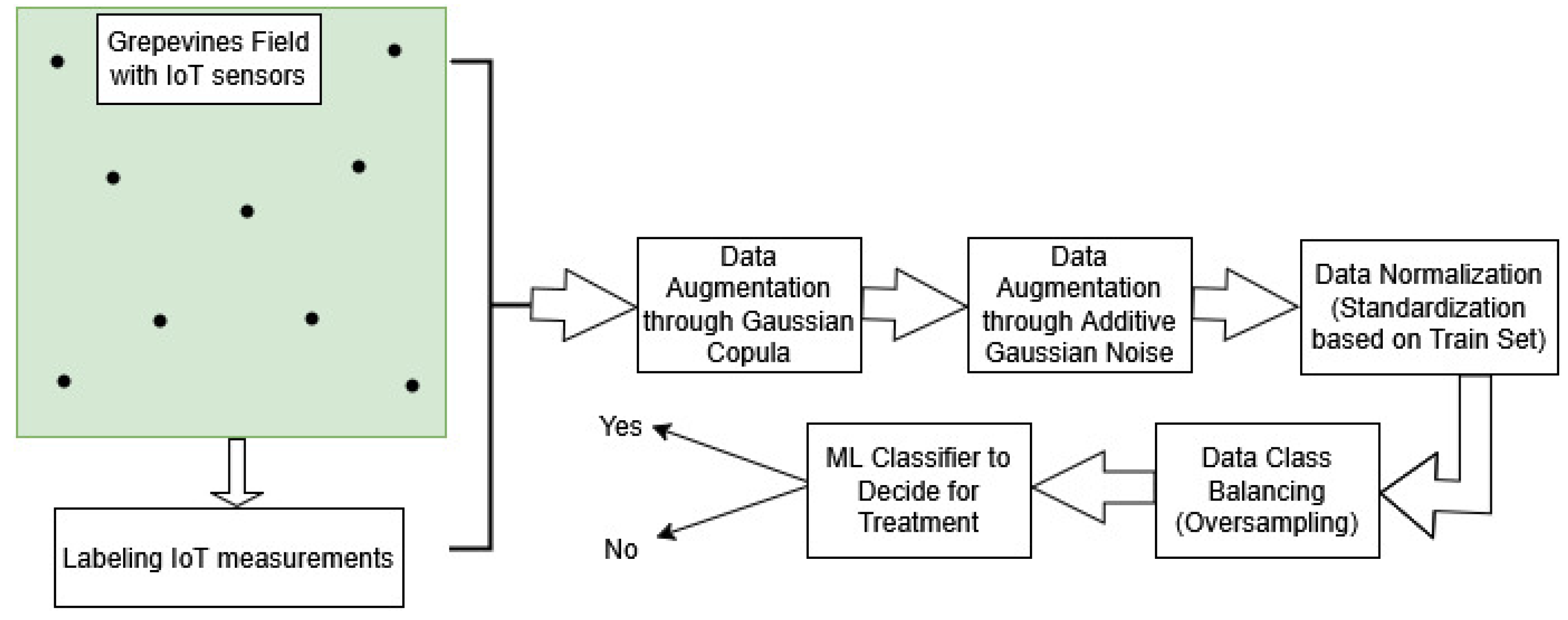
Figure 1.
The workflow of our suggested solution to predict whether there is highly possible to appear grapevines diseases caused by pathogens, based on environmental factors monitored by IoT sensors. The model decides whether there should be applied treatment or not.
Figure 1.
The workflow of our suggested solution to predict whether there is highly possible to appear grapevines diseases caused by pathogens, based on environmental factors monitored by IoT sensors. The model decides whether there should be applied treatment or not.
4.1. Data Description
4.1.1. Grapevines Field Description
The study was conducted in a 7-hectare experimental vineyard located in Tebano (Faenza, RA), Emilia-Romagna, Italy. The vineyard is situated on flat terrain with a clayey loam soil. It follows an integrated management approach, combining sustainable agronomic practices. The vineyard hosts multiple grapevine cultivars, including Sangiovese, Trebbiano, Pignoletto, Albana, Lambrusco Salamino, Lambrusco Sorbara, and Ancellotta, all grafted onto Kober 5BB rootstocks. The vines were planted in 2018 and are trained using the Guyot system. The planting layout consists of 2.7 meters between rows and 1 meter between vines within the same row. The vineyard is on a flat surface and oriented southwest. Irrigation is managed through a drip irrigation system, with an irrigation flow rate of 4 L/h and drippers spaced every 50 cm.
4.1.2. IoT Environmental Data Acquisition & Labeling
The environmental monitoring system used in this study was designed to collect and structure a multi-year dataset, covering the period from 1st of January 2020 to middle of May 2024. The data acquisition process involved two different weather stations, which ensured consistency in the recorded parameters over time. A weather station was usedmeasure key environmental variables, including air temperature, relative humidity and the amount of rain water in the soil. These parameters were recorded daily, providing an overview of the microclimatic conditions of the vineyard during different growing seasons.
All collected data, including meteorological, soil, and vineyard management records, were systematically processed and structured into standardized Excel files. To facilitate data analysis, the meteorological dataset was categorized with key attributes such as vineyard structure reference, company name, field identification, crop variety, and date of measurement. Environmental variables were further refined through statistical aggregations, including average, minimum, maximum, sum, deviation, mode, and median. This structured approach allowed for improved data interpretation and integration over multiple years.
In addition to meteorological monitoring, treatment applications were meticulously documented to establish a relationship between disease management interventions and previous climatic conditions. For each treatment, the dataset recorded the date of application, the type of product used, the dosage, the applied volume, and the target pathogen. An essential aspect of data annotation involved linking treatment events to preceding meteorological conditions. In the meteorological dataset, treatments were explicitly annotated, and for each application, environmental data from up to five days prior were also included. This methodology enabled the assessment of how climatic variations influenced disease development and, consequently, the timing and necessity of fungicide applications.
4.2. Data Augmentation & Preprocessing
One of the main reasons that ML models do not perform as well as they could is data scarcity and also the nature of real-data used to train a model. Often, real-data may be difficult to be captured/recorded in a sufficient amount to allow for model convergence. In addition, they may underepresent the situations of the task favoring one or some cases over the others. A way to increase the amount of data in a qualitative manner addressing data scarcity and improving the model’s generalization ability is to use synthetic data that mimic the properties of the original data; thus, we perform synthetic data generation using Gaussian Copula and Additive Gaussian Noise.
4.2.1. Gaussian Copula Based Synthetic Data Generation
Inspired by studies that worked on the generation of synthetic data for an ML emulator on environmental data [21], or suggested a Copula-based framework for the generation of synthetic data [22], we leveraged the efficiency of the properties of the simple statistical methods (multivariate CDF) of Gaussian Copula [19], to generate new synthetic data. The amount of the initial data was rather small to allow the model be trained properly on them. Gaussian Copula can model and estimate the (Gaussian) distribution of the features and find the inter-correlation among them. It does that by estimating the joint cumulative distribution function (joint CDF) of the features. A Gaussian Copula is constructed from a multivariate normal distribution with correlation matrix P. The reverse steps of the Copula computation are used to generate pseudo-random samples from general classes of multivariate probability distributions. In our case, that is, tabular data of environmental measurements, Copulas and their inverse transformation method, are very useful to produce a synthetic data set that mimics the real data in terms of association of their features [20].
4.2.2. Additive Gaussian Noise Based Synthetic Data Generation
Apart from augmenting data using Gaussian Copula, we also augmented data using Gaussian Noise. Generation of synthetic data using additive Gaussian Noise has already been explored on the original environmental data [23]. Gaussian Noise standard deviation was set to be 0.1 times the standard deviation of the original feature, for each feature column, as a value that allows to generate new features that are close to the original ones but also have a satisfying degree of variance.
4.2.3. Data Normalization (Standardization)
We performed normalization and specifically standardization which is a common method where each feature is transformed so that it has a mean value of zero and a standard deviation of one. Mean value and standard deviation were considered on training data. When features vary widely in scale (for example tabular data including age in years and also income in dollars), algorithms that use distance metrics (such as k-nearest neighbors or support vector machines) or gradient-based optimization (like neural networks and linear regression with gradient descent, again like in our case) can be biased toward features with larger magnitudes. Normalizing the features puts them on a comparable scale, ensuring that each feature influences the outcome in a similar manner, so it is an essential step before feeding the data to a model.
4.2.4. Data Balancing
It is something common in real-world applications to have imbalanced datasets, that is, instances of a class are much more than the other(s). This is also the case with this dataset and it is reasonable since pathogens occur when the environmental conditions foster their presence or when no treatment has been applied. SMOTE [24] algorithm was chosen for oversampling as a method to form a more balanced dataset.
Of course, we first splitted data to 80% train and 20% test and then we normalized and oversampled them based on train data. Before oversampling we had 1300 train data of which 988 belonged to class 0 (no disease) and 312 to class 1 (disease). After oversampling, the ratio of the minority class to the majority is 80%. The amount of train data was raised to 1778 of which 790 belonged to class 1 while the amount of class 0 data remained the same.
4.3. Grapevines Disease Prediction Using ML
We formed the pathogen prediction task as a binary tabular data classification problem and we used different classifiers to compare which performs better. The classifiers used were Logistic Regression Classifier, K-Nearest Neighbours, SVM Classifier, Random Forest, GradientBoosting, XGBoost, CatBoost and the recently released Transformer based Tab-PFN classifier. Next, we explain shortly the way we used each classifier.
4.3.1. Logistic Regression
Logistic Regression was used as a simple and fast baseline ML method. It is well suited to our problem as a statistical method that solves binary problems. As a solver to estimate the parameters of logistic regression, the LBFGS (Limited-memory Broyden–Fletcher–Goldfarb–Shanno algorithm) algorithm was used [26], which is an efficient optimization algorithm that uses limited memory resources.
4.3.2. KNN
K-Nearest Neighbour is the simplest ML classifier. Having stored examples from each class as training examples, the new test examples are compared in terms of distance with the training examples and the class assigned to each new example is that of the majority of the closest k neighbour examples. We set the number of neighbours equal to 3 and the distance function was Euclidean.
4.3.3. Support Vector Machine (SVM)
Since we have a binary classification task, SVM is also chosen as a supervised algorithm that tries to maximize the margin between the closest points of the two classes. The kernel of the classifier was Radial-Basis Function and the gamma parameter of the RBF function was set equal to the inverse of the number of features times the variance of the data.
4.3.4. Random Forest
A way to get stronger predictive results and robustness is to use ensemble methods like Random Forest. The creation of a multitude of decision trees during training often leads to stronger classification results. Experimentally, we found that 10 is the optimum maximum tree depth for our data.
4.3.5. GradientBoosting
Also an ensemble method, Gradient Boosting reveals its power by combining several weak learners into a strong learner, in which each new model is trained to minimize the loss function such as mean squared error or cross-entropy of the previous model using gradient descent. We set the number of estimators, that is the number of the trees in the ensemble, equal to 100 and the maximum depth of each tree equal to 8.
4.3.6. XGBoost
XGBoost [28] is a computationally optimized algorithm and powerful for structured or tabular data like our case. XGBoost is an extension of Gradient Boosting and was selected here for its very good performance in a wide range of classification tasks. We set its maximum tree depth equal to 5.
4.3.7. CatBoost
CatBoost [29], as an ensemble of decision trees, was chosen for many reasons. By using Ordered Target Statistics and Ordered Boosting, it can avoid data leakage; thus it is less possible to have overfitting. On tabular data, it performs similarly or even better with XGBoost and since it is a tree-based method it can provide some level of explainability; useful in a real application that a farmer may ask for clarification about the model’s output.
4.3.8. TabPFN Transformer
The aforementioned ML alorithms are known, so there is no need of explaining their functionality further. However, TabPFN [25] is a newly proposed tabular classification algorithm based on Prior-Fitted Network [30] which proves that a Transformer [27] network can approximate Bayessian Inference. TabPFN brings a radical new view on the way that tabular classification is done, as it provides fast and accurate results without requiring training.
Authors of [25] made slight modifications to the specific attention mask (proposed by [30]) of the Transformer encoder to make it yield faster inference with the same performance. Moreover, the TabPFN Transformer has no more any positional encoding; no need for them if the input is not sequential, but keep the zero-padding and a linear scaling to the features to allow the model accept inputs of variable length.
Except for its very good performance, TabPFN-Transformer has also the advantage of yielding predictions in less than a second; something important both in terms of sustainability since it allows for affordable and green ML and also on terms of time complexity making it a good choice for a real-time system.
4.4. Evaluation Metrics
Accuracy, which gives the proportion of the total predictions that were correct, is the typical metric in classification tasks. Apart from it, we also use ROC-AUC score, Precision, Recall and F1 as evaluation metrics, in order to have a better view of the models’ behavior and performance.
ROC-AUC score computes the Area Under the Curve (AUC) of the Receiver Operating Characteristic (ROC). ROC is a figure of sensitivity (true positive rate) over specificity (false positive rate). AUC measures the entire area under ROC curve. It is less influenced by changes in class distribution than accuracy. We used the weighted version of it which computes metrics for each label and finds their average, weighted by the number of true instances for each label.
Precision and Recall are useful since a high value of them indicates a few False Positives and a few False Negatives respectively. However, both the number of False Positives and False Negatives should be considered and F1-score integrates them as a harmonic mean of Precision and Recall.
We measure Precision, Recall and F1-Score evaluation metrics for both classes separately to see how the model behaves in each case; we are more interested in the minority class, that is, the case of actually existing a high risk of a grapevines disease.
5. Results
As mentioned above, we experimented with different ML prediction models on our collected and curated IoT tabular data. Some of the models were chosen as baseline methods, like Logistic Regression and KNN which are traditionally used on this task and others for their proven very good performance such as XGBoost [28], CatBosst [29] and also the state of the art TabPFN Transformer [25]. The results for predicting the risk of infection of each of the two diseases, downy mildew and powdery mildew are shown at Table 1 and Table 2.
Considering the results, Logistic Regression, SVM and KNN had a rather poor performance; after all, their usage was useful as baseline results. The problem seemed to be difficult to be solved succesfully for ensemble and boosting methods like Random Forest, Gradient Boosting, XGBoost and CatBoost. The problem became harder for those classifiers possibly due to the fact of labeling also a few more days before actually treatment was applied as high risk days of disease development. Our expectations were met with TabPFN-Transformer which was the only of the used classifiers that had high precision and recall results for the ’Yes’ class, the class that reveals high risk of disease presence or development.
6. Discussion
Our aim in this work was to suggest a way to develop a performance robust and real-time efficient to predict downy mildew and powdery mildew. Firstly, we wanted to see which ML Classifier performed better and then to compare their prediction time. Considering the results of Table 1 and Table 2, TabPFN-Transformer proved that can fit as a predictor in a real-time system.
Our IoT sensors monitored three environmental features, temperature, humidity and the amount of rain water remained at the soil. However, more environmental parameters play a key role in allowing pathogens to cause diseases in grapevines. Parameters like solar radiation, leaf wetness, soil moisture and temperature, wind speed and direction along with susceptible crop phenological stages and grapevine variety, could also be considered in order to have a more realistic modeling of the conditions under which the diseases are initially observed on the crops, progressing and affecting them. Such an environmental modeling would help to better distinguish environmental conditions that differ in a level that reveals different diseases or no disease at all.
Of course, it is crucial to monitor such environmental measurements for a long period and also keep a detailed record of when any treatment was applied to prevent diseases. Thus, quantitative and qualitative data would have been formed to help have an unbiased ML model with a good generalization ability eager to predict the appearance of a disease at any environmental conditions.
Nonetheless, with the current variety of IoT sensors and the TabPFN-Transformer our suggested system showed a very good performance, eager to be applied in real-conditions to perform early downy mildew and powdery mildew disease prediction. This is because of among the aforementioned environmental parameters that could be useful, temperature and humidity are the most significant for these two diseases’ prediction.
7. Conclusions
This study presented a workflow for predicting grapevines disease as an early warning based on environmental parameters. We explained the way downy mildew and powdery mildew diseases affect grapevines and the effect that specific environmental conditions have in the development of these diseases. The suggested workflow includes a full pipeline from collecting and labeling IoT sensor data, spanning from 2020 to May of 2024, augmenting and preprocessing data and driving them to the appropriate ML model to predict a disease and decide whether should be applied a fungicide treatment to prevent a disease or not. Despite its limitations, the real field data collected and used and the TabPFN-Transformer ML model, which can perform classification in less than a second, give our suggested solution high potential to be applicable to real conditions.
Author Contributions
Conceptualization, Nikolaos Arvanitis; Data curation, Filippo Graziosi; Formal analysis, Filippo Graziosi and Gina Athanasiou; Investigation, Nikolaos Arvanitis and Filippo Graziosi; Methodology, Nikolaos Arvanitis; Project administration, Theodore Zahariadis; Software, Nikolaos Arvanitis; Validation, Nikolaos Arvanitis; Writing – original draft, Nikolaos Arvanitis and Filippo Graziosi; Writing – review & editing, Gina Athanasiou, Antonia Terpou, Olga Arvaniti and Theodore Zahariadis.
Funding
This work has been funded by the European Commission through the HORIZON-RIA action under the Call HORIZON-CL6-2022-GOVERNANCE-01 and is running under the Grant Agreement 101086461 with project acronym: AgriDataValue, and project name: Smart Farm and Agri-environmental Big Data Value.
Data Availability Statement
The data used at this work are available at https://zenodo.org/records/14989522.
Conflicts of Interest
The authors declare no conflicts of interest.
Abbreviations
The following abbreviations are used in this manuscript:
| KNN | K-Nearest Neighbours |
| SVM | Support Vector Machine |
| TabPFN | Tabular Prior-Data Fitted Network |
References
- Patil, S. S. & Thorat, S. A. Early detection of grapes diseases using machine learning and IoT, 2016 Second International Conference on Cognitive Computing and Information Processing (CCIP), Mysuru, India, 2016, pp. 1-5. [CrossRef]
- Sanghavi, Kainjan & Sanghavi, Mahesh & Rajurkar, Archana M. Early stage detection of Downy and Powdery Mildew grape disease using atmospheric parameters through sensor nodes, Artificial Intelligence in Agriculture, Volume 5, 2021, Pages 223-232, ISSN 2589-7217. Available online: https://www.sciencedirect.com/science/article/pii/S2589721721000283. [CrossRef]
- Hnatiuc, Mihaela & Ghita, Simona & Alpetri, Domnica & Ranca, Aurora & Artem, Victoria & Dina, Ionica & Cosma, Mădălina & Mohammed, Mazin Abed. 2023. "Intelligent Grapevine Disease Detection Using IoT Sensor Network" Bioengineering 10, no. 9: 1021. [CrossRef]
- Gessler, C. & Pertot, I. & Perazzolli, M. (2011). Plasmopara viticola: a review of knowledge on downy mildew of grapevine and effective disease management. Phytopathologia Mediterranea, 50(1), 3–44. Available online: http://www.jstor.org/stable/26458675.
- Martinson, T. E. & Dunst, R. & Lakso, A. & English-Loeb, G. 1997. Impact of feeding injury by Eastern Grape Leafhopper (Homoptera:Cicadellidae) on yield and juice quality of Concord grapes. Amer. J. Enol. Vitic. 48:291-302.
- Thind, T.S. & Arora, J.K. & Mohan, C. & Raj, P. (2004). Epidemiology of Powdery Mildew, Downy Mildew and Anthracnose Diseases of Grapevine. In: Naqvi, S.A.M.H. (eds) Diseases of Fruits and Vegetables Volume I. Springer, Dordrecht. [CrossRef]
- Williamson, B. & Tudzynski, B. & Tudzynski, P. & van Kan JA. Botrytis cinerea: the cause of grey mould disease. Mol Plant Pathol. 2007 Sep;8(5):561-80. [CrossRef] [PubMed]
- Gadoury, David. (1997). Effects of environment and fungicides on epidemics of grape powdery mildew: considerations for practical model development and disease management. Viticultural and Enological Science. 52. 225-229.
- Gadoury, David & Seem, Robert & Pearson, Roger & Wilcox, Wayne & Dunst, Richard. (2001). Effects of Powdery Mildew on Vine Growth, Yield, and Quality of Concord Grapes. Plant Disease - PLANT DIS. 85. 137-140. [CrossRef]
- Pool, R. M. & Pearson, R. C. & Welser, M. J. & Lasko, A. N & Seem, R. C. 1984. Influence of powdery mildew on yield and growth of rosette grapevine. Plant Disease, 68: 590-593.
- Rao, K.C, 1992. Epidemiology of some common diseases of grape around Hyderabad. In: “Proceedings of International Symposium on Recent Advances in Viticulture and Oenology, Hyderabad, India”, pp 323-329.
- Willocquet, Laetitia & Berud, F. & Raoux, L. & Clerjeau, Michel. (2007). Effects of wind, relative humidity, leaf movement and colony age on dispersal of conidia of Uncinula necator, causal agent of grape powdery mildew. Plant Pathology. 47. 234 - 242. [CrossRef]
- Koledenkova, K. & Esmaeel, Q. & Jacquard, C. & Nowak, J. & Clément, C. & Ait Barka, E. (2022) Plasmopara viticola the Causal Agent of Downy Mildew of Grapevine: From Its Taxonomy to Disease Management. Front. Microbiol. 13:889472. [CrossRef]
- Velasquez-Camacho, L. & Otero, M. & Basile, B. & Pijuan, J. & Corrado, G., Current Trends and Perspectives on Predictive Models for Mildew Diseases in Vineyards. Microorganisms. 2022 Dec 27;11(1):73. [CrossRef] [PubMed] [PubMed Central]
- Peng, J. & Wang, X. & Wang, H. & Li, X. & Zhang, Q. & Wang, M. (2024) Advances in understanding grapevine downy mildew: From pathogen infection to disease management. Molecular Plant Pathology, 25, e13401. [CrossRef]
- Fernandes de Oliveira, A. & Serra, S. & Ligios, V. & Satta, D. & Nieddu, G. (2021). Assessing the Effects of Vineyard Soil Management on Downy and Powdery Mildew Development. Horticulturae, 7(8), 209. [CrossRef]
- Ricciardi, Valentina & Crespan, Manna & Maddalena, Giuliana & Migliaro, Daniele & Brancadoro, Lucio & Maghradze, David & Failla, Osvaldo & Toffolatti, Silvia Laura & De Lorenzis, Gabriella, Novel loci associated with resistance to downy and powdery mildew in grapevine, Frontiers in Plant Science, vol.15, 2024. Available online: https://www.frontiersin.org/journals/plant-science/articles/10.3389/fpls.2024.1386225ISSN 1664-462X. [CrossRef]
- Bois, B. & Zito, S. & Calonnec, A. (2017). Climate vs grapevine pests and diseases worldwide: the first results of a global survey. OENO One, 51(2), 133–139. [CrossRef]
- Nelsen, R. B. An introduction to Copulas, Springer Science & Business Media, 2006.
- Houssou, Regis & Augustin, Mihai-Cezar & Rappos, Efstratios & Bonvin, Vivien & Robert-Nicoud, Stephan. (2022) Generation and Simulation of Synthetic Datasets with Copulas. Available online: https://arxiv.org/abs/2203.17250.
- Meyer, David & Nagler, Thomas & Hogan, Robin. (2020). Copula-based synthetic data generation for machine learning emulators in weather and climate: application to a simple radiation model. [CrossRef]
- Li, Zheng & Zhao, Yue & Fu, Jialin. (2020). SYNC: A Copula based Framework for Generating Synthetic Data from Aggregated Sources. [CrossRef]
- Bilali, A.E & Taleb, A. & Bahlaoui, M. A. & Brouziyne, Y. An integrated approach based on Gaussian noises-based data augmentation method and AdaBoost model to predict faecal coliforms in rivers with small dataset, Journal of Hydrology, Volume 599, 2021, 126510. ISSN 0022-1694. [CrossRef]
- Chawla, Nitesh V. & Bowyer, Kevin W. & Hall, Lawrence o. & Kegelmeyer, Philip W., (2002). Smote: synthetic minority over-sampling technique. Journal of artificial intelligence research 2002 16:321–357.
- Hollmann, N. & Müller, S. & Eggensperger, K. & Hutter, F., (2023). TabPFN: A Transformer That Solves Small Tabular Classification Problems in a Second. Available online: https://arxiv.org/abs/2207.01848.
- Liu, D.C. & Nocedal, J. On the limited memory BFGS method for large scale optimization. Mathematical Programming 45, 503–528 (1989). [CrossRef]
- Vaswani, A. & Shazeer, N. & Parmar, N. & Uszkoreit, J. & Jones, L. & Gomez, A. & Kaiser, L. & Polosukhin I. Attention is all you need. In I. Guyon, U. von Luxburg, S. Bengio, H. Wallach, R. Fergus, S. Vishwanathan, and R. Garnett, editors, Proceedings of the 30th International Conference on Advances in Neural Information Processing Systems (NeurIPS’17). Curran Associates, Inc., 2017.
- Chen, Tianqi & Guestrin, Carlos. 2016. XGBoost: A Scalable Tree Boosting System. In Proceedings of the 22nd ACM SIGKDD International Conference on Knowledge Discovery and Data Mining (KDD ’16). Association for Computing Machinery, New York, NY, USA, 785–794. [CrossRef]
- Prokhorenkova, Liudmila & Gusev, Gleb & Vorobev, Aleksandr & Dorogush, Anna-Veronika & Andrey Gulin. 2018. CatBoost: unbiased boosting with categorical features. In Proceedings of the 32nd International Conference on Neural Information Processing Systems (NIPS’18). Curran Associates Inc., Red Hook, NY, USA, 6639–6649.
- Müller, S & Hollmann, N. & Arango, S. & Grabocka, J. & Hutter, F. Transformers can do bayesian inference. In Proceedings of the International Conference on Learning Representations (ICLR’22), 2022. Published online: iclr.cc. Available online: https://openreview.net/forum?id=KSugKcbNf9.

Table 1.
Downy mildew Disease Classification Results.
| Classifier | Accuracy | ROC-AUC | Precision | Recall | F1-Score | |||
| No | Yes | No | Yes | No | Yes | |||
| Logistic Regression | 0.6125 | 0.6062 | 0.8058 | 0.3637 | 0.6299 | 0.5942 | 0.7017 | 0.4628 |
| KNN | 0.7849 | 0.7632 | 0.8861 | 0.5902 | 0.8099 | 0.7162 | 0.8464 | 0.6509 |
| SVM | 0.6987 | 0.6788 | 0.8351 | 0.4675 | 0.7339 | 0.6251 | 0.7807 | 0.5285 |
| Random Forest | 0.8576 | 0.8245 | 0.9082 | 0.7361 | 0.8959 | 0.7530 | 0.9021 | 0.7394 |
| GradientBoosting | 0.8742 | 0.7969 | 0.8816 | 0.8437 | 0.9585 | 0.6352 | 0.9184 | 0.7248 |
| XGBoost | 0.8379 | 0.7648 | 0.8645 | 0.7428 | 0.9231 | 0.6153 | 0.8977 | 0.6973 |
| CatBoost | 0.8642 | 0.8112 | 0.8846 | 0.7942 | 0.9365 | 0.6785 | 0.9098 | 0.7249 |
| TabPFN Transformer | 0.9669 | 0.9461 | 0.9648 | 0.9733 | 0.9801 | 0.9014 | 0.9773 | 0.9359 |
Table 2.
Powdery mildew Disease Classification Results.
| Classifier | Accuracy | ROC-AUC | Precision | Recall | F1-Score | |||
| No | Yes | No | Yes | No | Yes | |||
| Logistic Regression | 0.5767 | 0.5917 | 0.8047 | 0.3375 | 0.5665 | 0.6162 | 0.6652 | 0.4462 |
| KNN | 0.7731 | 0.7674 | 0.8990 | 0.5509 | 0.7791 | 0.7558 | 0.8348 | 0.6376 |
| SVM | 0.5736 | 0.6283 | 0.8482 | 0.3632 | 0.5226 | 0.7441 | 0.6391 | 0.4892 |
| Random Forest | 0.8190 | 0.7838 | 0.8917 | 0.6423 | 0.8583 | 0.7094 | 0.8747 | 0.6742 |
| GradientBoosting | 0.7147 | 0.6383 | 0.8101 | 0.4606 | 0.8000 | 0.4868 | 0.8050 | 0.4785 |
| XGBoost | 0.8220 | 0.7374 | 0.8527 | 0.7059 | 0.9165 | 0.5681 | 0.8835 | 0.6333 |
| CatBoost | 0.8344 | 0.7345 | 0.8690 | 0.7162 | 0.9125 | 0.6283 | 0.8902 | 0.6725 |
| TabPFN Transformer | 0.9202 | 0.8713 | 0.9212 | 0.9166 | 0.9740 | 0.7973 | 0.9473 | 0.8653 |
Disclaimer/Publisher’s Note: The statements, opinions and data contained in all publications are solely those of the individual author(s) and contributor(s) and not of MDPI and/or the editor(s). MDPI and/or the editor(s) disclaim responsibility for any injury to people or property resulting from any ideas, methods, instructions or products referred to in the content. |
© 2025 by the authors. Licensee MDPI, Basel, Switzerland. This article is an open access article distributed under the terms and conditions of the Creative Commons Attribution (CC BY) license (https://creativecommons.org/licenses/by/4.0/).
Copyright: This open access article is published under a Creative Commons CC BY 4.0 license, which permit the free download, distribution, and reuse, provided that the author and preprint are cited in any reuse.


