
Submitted:
11 March 2025
Posted:
12 March 2025
You are already at the latest version
Abstract
Hematoxylin and Eosin (HE) staining is gold standard in histopathological examination of cancer tissue, representing first step towards cancer diagnosis. Second step is series of immunohistochemical stainings, including cell proliferation marker called Ki67 index. Deep learning models offer promising solutions for improving medical diagnostics, while generative models provide additional explainability of predictive models, which is essential for their adoption in clinical practice. Our previous work introduced novel approach that utilises conditional StyleGAN model for generating HE-stained images conditioned on Ki67 index. This study proposes to employ this model for generating sequences of HE-stained images reflecting varying Ki67 index values. Sequences enable exploration of hidden relationships between HE and Ki67 staining and can enhance explainability of predictive models, e.g., by generating counterfactual examples. While our previous research focused on assessing quality of generated HE images, this study extends that work by evaluating model’s ability to capture Ki67-related variations in HE-stained images. Additionally, expert pathologists evaluated generated sequences, proposing criteria for assessing their relevance. Our findings demonstrate potential of conditional StyleGAN model as part of explainable framework for analysing and predicting immunohistochemical information from HE-stained images. Results highlight relevance of generative models in histopathology and their potential applications in cancer progression analysis.
Keywords:
Hematoxylin and Eosin
; Ki67
; Conditional GAN
; StyleGAN
; Digital Pathology
1. Introduction
Histopathology is the study that involves an examination of tissue sections stained by different methods using light microscopy to identify signs of disease [1]. Histopathological analysis represents a condition sine qua non in cancer diagnosis, tumour exact classification and subsequent treatment recommendations. Tissue staining is a technique that applies one or more dyes to tissue sections to enhance contrast and help pathologists identify different diagnostically relevant morphological features of the examined cells. Hematoxylin and Eosin (HE) staining is a gold standard in tissue cancer diagnosis, which highlights different microscopically evaluable pathological changes of cancer cells different from those of normal cells in a stained tissue section. Immunohistochemical (IHC) stainings are used to specify the type of cancer by employing antibodies to detect lineage and or differentiation and prognostic specific antigens (markers) within cancer tissue sections. In addition, the Ki67 antigen serves as a marker of cell proliferation, assessing Ki67-positive cells that are abnormally growing and dividing, thereby possibly indicating the rate of tumour growth. The Ki67 index quantifies the expression of Ki67-positive cells by calculating the percentage of positive cancer cells in a tissue section. The evaluation of the Ki67 index represents a mandatory step in the cancer diagnostic algorithm; however, the IHC Ki67 staining is more resource and time-demanding, and its evaluation is more time-consuming than those of HE staining.
Deep learning models show promise for improving medical diagnostics. They can provide fast, consistent, and cost-effective decision-making. However, errors in medical contexts can lead to serious consequences. Therefore, these models must be explainable before their implementation in clinical practice to prevent potential failures or reveal biases. Model explainability provides transparency, fairness, accuracy, generality, and comprehensibility to the results [2]. Furthermore, the General Data Protection Regulation (GDPR) [3] issued by the European Union requires the transparency of an algorithm before it can be used in patient care.
Integrating a generative model into a deep learning framework can improve explainability by providing additional information to support model predictions. For instance, generative models can produce counterfactual examples, which are derived from minimal modifications to the original data that result in a change in the model’s prediction, such as a label shift from healthy to unhealthy in the context of medical image analysis. According to [4], pathologists consider counterfactual examples as offering adequate insight into the algorithm’s decision-making criteria. Furthermore, generative models can improve deep learning model performance by augmenting training data [5].
In our previous works [6,7], we proposed the conditional StyleGAN model for generating synthetic HE-stained images conditioned on the Ki67 index, demonstrating promising results in producing realistic synthetic image patches. However, these works primarily focused on the quality of generated HE images without addressing the Ki67 information obtained from them. In this paper, we extend our analysis by evaluating the Ki67 information within synthetic HE images, aiming to use our model to modify HE images to reflect varying Ki67 index values. Furthermore, we generate sequences of HE-stained images with progressively changing Ki67 index values to analyse the relationship between HE and Ki67 staining.
Our research aims to develop an explainable framework for predicting the Ki67 index from HE-stained histological images, with the explainability achieved through the use of generative models. The conditional generative model from this paper can be further employed in this explainable framework to explain the Ki67 index predictions from HE-stained images by generating counterfactual examples and simulating cancer progression. Additionally, it can provide deeper insights into the relationship between HE and Ki67 stainings.
The paper is organised as follows. In Section 2, we discuss generative models and related works. Section 3, describes the dataset, conditional generative model and evaluation metrics. Section 4 evaluates the model and its latent space and analyses Ki67 information in HE-stained images. Finally, Section 5 presents conclusions and outlines potential directions for future research.
2. Background
2.1. Generative Adversarial Networks
Generative Adversarial Network (GAN), introduced by Goodfellow et al. [8], is based on the principle of a min-max optimisation game involving two competing models: a generator G and a discriminator D. The generator aims to learn the distribution of real data and, subsequently, generate new synthetic samples from this learned distribution that closely resemble the real data. In contrast, the discriminator is trained to distinguish between real data from the real dataset and synthetic data produced by the generator. Both models are trained concurrently, thus improving simultaneously; as the generator produces more realistic samples, the discriminator improves its ability to accurately differentiate between real and generated data.
The training dataset represents a high-dimensional probability distribution of real data that the generator learns to approximate without explicit specification; thus, it learns this distribution directly from the data samples. As specified by Goodfellow et al. [8], the generator is trained to map a random latent vector drawn from a prior distribution (typically Gaussian or uniform), into a complex distribution approximating real data. The generator is typically implemented as a neural network or convolutional neural network for image data, taking a latent vector as input and outputting a synthetic data sample. In contrast, the discriminator is typically designed as a classification neural network or convolutional neural network that assesses the credibility of input samples, providing a probability score indicating the likelihood that a given sample is real.
GAN models are capable of generating a large number of realistic data samples that closely resemble the training data. However, they are often associated with several problems, including issues with convergence or vanishing gradients. Another common issue is mode collapse, when the generator produces only a limited subset of data distribution, manifesting as a lack of diversity in the generated output [9].
Several variations of the original GAN model have been proposed. Conditional GAN incorporates additional information into both the generator and the discriminator. It enables the model to generate data conditioned on a specific class label, thereby providing more control over the generation process. The concept of conditional GAN was introduced in the original GAN paper by Goodfellow et al. [8]. However, it was explored in more detail in the subsequent paper by Mirza et al. [10].
StyleGAN is another improved version of the GAN model introduced by Karras et al. [11]. It improves image quality and the structure of latent space, automatically disentangling high-level features, resulting in a more interpretable latent space and providing higher control over the image generation process. StyleGAN involves enhanced generator and discriminator architecture. The generator comprises two networks: a mapping network and a synthesis network. Firstly, the non-linear mapping network maps latent vectors from input latent space to intermediate space. This intermediate space is disentangled and not shape-limited [11], allowing the capture of more meaningful feature representations. Secondly, the progressively growing synthesis network enables the generation of high-resolution images with reduced training time.
2.2. Related Work
Several studies have employed generative models in the histopathology domain. Daroach et al. [12] utilised StyleGAN to generate high-resolution synthetic HE-stained images of prostatic tissue. Leveraging StyleGAN progressive growing, the model effectively captured histopathological features across various magnifications, with generated images deemed nearly indistinguishable from real samples by expert pathologists. In their style mixing experiments, Daroach et al. observed that StyleGAN’s hierarchical architecture allowed for specific control over image features: coarse layers determine large structures (gland and lumen locations), middle layers define epithelium and stroma textures, and fine layers adjust colour and nuclear density. Furthermore, researchers explored StyleGAN’s latent space through several experiments. They determined representatives for eight histopathological classes by averaging latent vectors of the sample of generated images assigned to the same class. These representatives were proven to successfully mimic real histopathological features. Researchers further experimented with interpolation between images with different labels. Although the shortest path in latent space yielded realistic images, it did not align with natural biochemical tissue changes. Nevertheless, Daroach et al. demonstrated that the StyleGAN model can generate high-resolution histological images.
In related work, Daroach et al. [13] demonstrated that the latent space of a StyleGAN model, trained on a prostate histology dataset of patches, can capture pathologically significant semantics without data annotations. In the study, researchers generated a sample of synthetic images with known latent vectors, which were subsequently annotated by pathologists. Using these annotations, they identified distinct Gleason pattern-related regions within the latent space by applying principal component analysis. This allowed the generation of new synthetic images from these regions, preserving the diagnostic features of each region. Pathologists classified images generated from these regions, with of images aligning with the Gleason grade of their region and matching either the same or adjacent diagnostic region. Results indicate that StyleGAN successfully disentangled prostate cancer features consistently with Gleason grading, even without annotated training data. However, the researchers emphasised that a balanced training dataset significantly improves the latent space quality.
Quiros et al. [14] introduced PathologyGAN, a model capable of generating patches of HE-stained histological images validated by expert pathologists. PathologyGAN is built on the BigGAN architecture [15] with few modifications. It incorporates the Relativistic Average Discriminator [16] and several StyleGAN [11] features, including intermediate latent space, style mixing regularisation, and adaptive instance normalisation. PathologyGAN was trained on colorectal and breast cancer datasets. Researchers verified that it constructed the interpretable latent space that captures relevant tissue characteristics and allows transformations of semantic tissue features through linear vector operations. Additionally, linear interpolation between benign and malignant tissues showed a realistic growing number of cancer cells rather than their fading. In [17], Quiros et al. extended their previous work by incorporating the encoder to map real images into latent space, which allows the analysis of their feature representations in the subsequent paper [18].
Schutte et al. [19] proposed the interpretability method to explain black-box model predictions by generating sequences of synthetic images, illustrating the progression of pathology. The method consists of three parts: StyleGAN to generate synthetic images, the encoder to retrieve a latent representation of generated images, and the logistic regression classifier to approximate the original model’s predictions for generated images. A sequence is generated by traversing the shortest path in StyleGAN latent space, which results in a different model prediction. This approach enables us to observe changes that impact original model predictions, potentially uncovering new biomarkers [19]. Tested on knee X-rays, the method produced realistic X-ray sequences following osteoarthritis progression. Considering the dataset of breast cancer HE-stained patches, the model generated realistic tumour progression; however, the encoder could not perfectly reconstruct the original histological images.
The studies described above have focused primarily on HE staining without considering IHC. One promising approach is virtual staining, which transforms HE-stained images into IHC-stained images, enabling IHC analysis without the need for physically stained tissue sections. In this context, Chen et al. [20] introduced the Pathological Semantics-Preserving Learning method for Virtual Staining (PSPStain), specifically designed to preserve essential pathological semantics during the transformation process. Experimental results indicate that PSPStain outperforms existing HE-to-IHC virtual staining methods.
Our previous research [6,7] focused on generating HE-stained tissue images conditioned on the Ki67 index using the conditional StyleGAN model. In paper [7], we evaluated the training progress and synthetic image quality of several models, analysing the effects of two critical factors: the quality of the training dataset and the training duration. First, we compared results across two datasets—one containing only high-quality HE-stained patches with sufficient visible cells and the second comprising a broader range of patches, including lower-quality patches and those with fewer visible cells. Second, we compared different training durations to assess their impact on model performance. Additionally, generated images were reviewed and evaluated by the expert pathologist.
While our previous paper deeply analysed the quality of generated images, evaluating Ki67 information hidden in HE images is more challenging. In this paper, we complete the evaluation of this conditional model, incorporating the analysis of latent space and the evaluation of the conditional generator from different aspects. Moreover, we generate sequences of HE-stained images with the changing values of the Ki67 index and analyse the relationship between HE and Ki67 staining.
Several of the presented approaches addressed the simulation of cancer progression in histological images. Daroach et al. [12] and Quiros et al. [14] performed interpolation within the latent space between latent vectors of two different images. Schutte et al. [19] adopted the logistic regression classifier to identify the direction in latent space to change the image label. In contrast, our approach modifies the original image by adjusting the conditioning input for the conditional generator.
3. Methods
We use the conditional StyleGAN model presented in the paper [7], where we provided a detailed analysis of the image generation quality and validation by the pathologist. In that work, the expert pathologist confirmed the quality of the synthetic images, describing them as highly realistic. Synthetic images could only be distinguished from real ones upon close, detailed examination. However, that work omits the analysis of Ki67 information within generated HE-stained images and the analysis of latent space. Thus, in this paper, we conduct a detailed evaluation of these aspects.
3.1. Dataset
We employ the dataset presented in our paper [21]. The unprocessed histopathological dataset was provided by the Department of Pathology, Jessenius Medical Faculty of Comenius University and University Hospital Martin. It consists of HE and Ki67-stained whole slide images of seminoma, testicular tumour. This dataset comprises 77 pairs of HE-stained and Ki67-stained digital tissue scans, with each pair created from adjacent tissue sections. Although the sections do not match exactly at the cellular level, we assume that tissue sections from the same region share similar characteristics. Consequently, Ki67-stained images can be utilised to annotate their adjacent HE-stained images.
In this paper, we use the processed dataset initially introduced in our previous work [22] and subsequently employed to train the conditional StyleGAN model in [6,7]. The processed dataset was prepared through the semi-automated annotation approach since the unprocessed dataset lacked annotations. This process involved three main steps: tissue registration, colour-based clustering, and Ki67 index quantification. Due to the large size of whole slide images and computational constraints, the images were divided into smaller square patches at the second-highest resolution level. Corresponding HE and Ki67 patches were cut from the same position. Each HE patch was subsequently labelled with the Ki67 index, computed as the proportion of positively stained (brown) pixels in the corresponding clustered Ki67 patch. Figure 1 illustrates an example of an HE patch with the corresponding Ki67 patch, along with the Ki67 patch after clustering. Ki67 index of this patch is ().
To ensure the quality and relevance of patches, we applied the comprehensive filtering process, the details of which will be presented elsewhere. The filtering involved edge detection, blur detection, blob detection, and clustering techniques to exclude patches with lower quality or insufficient cellular content. As a result, the filtered dataset consists of 177,907 patches derived from 77 tissue scans, with each HE-stained patch labelled with its corresponding Ki67 index. Figure 2 illustrates an example of HE patches included in the filtered dataset, along with their corresponding Ki67 patches and Ki67 index labels. Figure 3 shows example patches that were excluded by the filtering process.
3.2. Generative Model
We utilise the generative model introduced in our earlier work [7]. Specifically, it is the conditional StyleGAN model that generates HE-stained image patches conditioned on the Ki67 index. The model is illustrated in Figure 4. It takes as input a latent vector and a specified Ki67 index to condition the generation of the HE-stained patch.
Daroach et al. [12] successfully applied StyleGAN [11] and StyleGAN2 [23] for histopathology image synthesis, which motivated our choice of their improved alias-free successor, StyleGAN3, proposed by Karras et al. [24]. Specifically, we adopt the StyleGAN3-R variant, which maintains equivariance to both translation and rotation that is convenient for histological images.
The model was trained using the official implementation from NVlabs [25], with a regularisation parameter gamma set to 2 and adaptive discriminator augmentation enabled. Training was conducted on the filtered dataset, which consists of the pairs of HE image patches and their corresponding Ki67 index values. For most experiments, we utilise the model trained for 5343 kimgs, indicating that the model processed 5343000 HE patches during the training phase; thus, it iterated through the whole dataset approximately 28 times. In a few experiments, we also employ the model trained for 10000 kimgs and compare its performance with the 5343 kimgs model.
3.3. Evaluation Metrics
We use three metrics—Fréchet Inception Distance, Fréchet Histological Distance, and Perceptual Path Length—to evaluate the generative model’s performance considering the quality of the generated images and the latent space. All these metrics are minimised for more realistic generated images and improved latent space quality. Together, these metrics provide a comprehensive evaluation of synthetic histological images by assessing visual and histological fidelity, diversity, and latent space disentanglement.
Fréchet Inception Distance (FID) [26] offers a quantitative assessment of how closely generated images approximate real-world data in terms of quality and diversity. This metric evaluates images based on high-level feature representations [27] from a pretrained Inception model, which aligns with human judgment. Specifically, FID measures the distance between the distributions of generated and real images by calculating the Fréchet distance [28] between two Gaussian distributions.
The second metric, Fréchet Histological Distance (FHD), is a modified FID designed specifically for histological images. Since the Inception model was trained on ImageNet, it does not consider histological features. To address this, we replace the Inception model with a histological model. Consequently, images are represented as high-level features of the histological model [22], which was trained to predict the Ki67 index from HE-stained images.
Perceptual Path Length (PPL) was introduced with the StyleGAN model [11] to evaluate the quality of latent space. It assesses the entanglement of latent space by quantifying the perceptual smoothness of interpolation between latent vectors. The perceptual distance between two images is calculated using VGG16 [29] embeddings.
4. Results
In this Section, we evaluate the conditional generator and its latent space, with a focus on the Ki67 index. Then, we propose the sequences of HE-stained images generated by modifying the Ki67 index and analyse the relationship between the generated HE images and their corresponding Ki67 index values.
4.1. Analysis of Training Progress
In the previous paper [7], we demonstrated that the model achieves superior results on the high-quality filtered dataset, particularly in terms of image quality and training stability. Figure 5 illustrates the FID and PPL progression during the training of this model. It is evident that while FID decreases as expected, PPL shows an increasing trend. The increase in PPL is likely due to the model overfitting to data; hence, the distance between real and synthetic data distribution is decreasing, but the latent space is getting more entangled. Besides, this phenomenon may be linked to mode collapse, where the model generates a limited variety of images.
While Figure 5 suggests that the model trained for 2000 kimgs achieves low values for both FID and PPL, visual inspection revealed that the generated images were less realistic. Expert pathologists evaluated images as realistic only after 5000 kimgs of training. Consequently, we selected the model with the training duration of 5343 kimgs for most of the subsequent experiments, as indicated by the vertical line in the Figure. This choice represents a compromise between FID and PPL, achieving a balance between image quality and latent space structure. Specifically, this model achieves the FID score of and the PPL of .
4.2. Evaluation of Conditional Generator
A conditional generator generates data with a specified property. In our case, we generate HE-stained histological images with the specified Ki67 index. To evaluate whether Ki67 information is obtained in generated HE images, we compared real images from our dataset with synthetic images produced by the conditional generator using various Ki67 intervals.
Ki67 index values are within the range. To evaluate the generator’s ability to generate HE-stained images with the specific Ki67 indexes, we divided the full Ki67 range into smaller Ki67 intervals, which were chosen as follows: , , , , , . The use of Ki67 index intervals for seminoma tumours is not standardised, and there is no consensus regarding the optimal cut-off values. Therefore, intervals were defined based on pathologists’ recommendations and considering the dataset distribution over Ki67 index labels. Certain intervals are hierarchical, where one interval is a subset of another, while others are complementary, thus representing non-overlapping data sets. The hierarchy of intervals is illustrated in Figure 6.
Before evaluating the generator, we assigned the real HE-stained images from our dataset to defined Ki67 intervals according to their Ki67 index labels. The distribution of real data across Ki67 intervals in the dataset is shown in Figure 7. We can observe that the Ki67 index labels are highly imbalanced, with the majority of the data labelled with the Ki67 index below , while only of the data have the Ki67 index above . Secondly, we created synthetic generator Ki67 intervals by randomly generating synthetic HE images for each Ki67 interval using our conditional generator. For each evaluation, we generated new 50000 synthetic HE images. Finally, we analysed the relationships between the dataset and the generator Ki67 intervals to assess the generator’s conditional performance.
4.2.1. Evaluation Using Fréchet Inception Distance
In the first evaluation of the generator’s performance, we scrutinised the visual similarity between Ki67 intervals. For this purpose, we adopted the Fréchet Inception Distance score, which measures the difference in the feature distribution between real and generated data using the inception model. FID scores were calculated between all dataset Ki67 intervals of real images and all generator Ki67 intervals of synthetic images generated by the conditional generator. The results are presented in Table 1, where rows correspond to dataset intervals, while columns represent generator intervals; hence, the values in the Table are not symmetric. We highlight the hierarchical structure of intervals in row and column descriptions through different colours.
Each value in the Table represents the FID score calculated between images from the corresponding real and generated intervals, reflecting the distance between their feature distributions. Lower FID scores indicate more similar distributions, suggesting that images from the generated interval more closely resemble those from the dataset interval. Lower FID scores are expected between subset intervals, highlighted with a green background in the Table. Conversely, higher FID scores, expected for complementary intervals, are distinguished with a yellow background. Unexpected FID scores are emphasised with red-coloured text. The lowest FID scores are anticipated along the Table’s diagonal, where the real and generated intervals are identical. These diagonal FID scores are marked in bold. Appendix A includes Table A1, which complements Table 1 by presenting FID scores with a heatmap background for a more intuitive visualisation of FID score differences.
When we analyse the results presented in Table 1, it is evident that the interval is complementary to all other intervals. As expected, the lowest FID score is found along the diagonal. When comparing the dataset interval with all generator intervals in the row, the interval exhibits the closest FID score to the diagonal, corresponding to the closest interval in terms of Ki67 distribution.
Next, we analyse the interval . As anticipated, the FID score with the complementary interval is high. The remaining intervals are subsets of , and, as expected, FID scores are lower compared to the complementary interval . The highest FID score is associated with the interval , but it is still more than two times lower than the score for the complementary interval . This is due to the fact that the majority of the real dataset within the interval consists of images with low Ki67 index values.
The Ki67 interval exhibits the least favourable performance in the Table. For the generator interval in the column, the FID score with the complementary dataset interval is lower than the diagonal score, indicating that the generated images are more similar to real images from the interval than to those from the interval. Furthermore, the dataset interval in the row shows a shorter distance to complementary intervals , , and . This can be attributed to the imbalanced distribution of the real data. However, the interval exhibits the expected high FID score with the complementary interval and the expected low score with .
The remaining intervals - , , and - have FID scores as expected, with lower values for subset intervals and higher values for complementary intervals. These intervals, along with , exhibit the lowest diagonal FID scores as they contain the majority of real data. In contrast, the interval has the highest diagonal FID as it contains the smallest number of real HE images. Therefore, the conditional generator demonstrates the highest performance in terms of visual similarity for the lower Ki67 index values.
4.2.2. Evaluation Using Fréchet Histological Distance
In addition to visual similarity, we evaluated the histological similarity between Ki67 intervals using Fréchet Histological Distance. FHD quantifies the distance between the feature distributions of real and generated HE images using the histological model.
FHD results for dataset vs. generator Ki67 intervals are summarised in Table 2, which follows the same structure as described in Section 4.2.1. Additionally, Table A2 in Appendix A presents FHD values with a heatmap background for enhanced visual representation. FHD results are proportionally similar to FID scores in Table 1, but slightly improved. Although the generator interval in the column again shows a lower distance to the dataset interval than the diagonal FHD score, the dataset interval in the row has the lowest FHD score along the diagonal, as expected. However, the diagonal FHD for the interval remains significantly higher than the diagonal FHD of other intervals.
Subsequently, we evaluated FHD scores for generator vs. generator to verify that the generator captures relevant histological characteristics for specific Ki67 intervals. The results are presented in Table 3 and in heatmap Table A4 in Appendix A. Tables follow the same structure as the previous Tables in this Section. However, in this case, both the rows and columns represent generator intervals, making the Table symmetric. The results are analogous to the dataset vs. generator where interval shows a smaller distance to the complementary interval than to . Aside from this, all other results align with expectations.
Additionally, we evaluated FHD scores for dataset vs. dataset Ki67 intervals to verify also the properties of our dataset. The results are summarised in Table 4 and heatmap Table A3 in Appendix A. Tables have a similar structure to the generator vs. generator Tables, but both the rows and columns correspond to dataset intervals, making this Table symmetric as well. The results reflect the Ki67 imbalance in the dataset, with the most accurate results observed for the lower Ki67 indices. However, the only notable inconsistency is that the Ki67 interval appears more similar to the complementary interval than to , which is a consequence of the majority of data in the interval having Ki67 labels close to 0. This inconsistency is also reflected in the behaviour of our conditional generator and thus can be observed in all the previously presented Tables.
4.2.3. Evaluation Using Perceptual Path Length
Besides visual and histological similarity, we analysed the conditional properties of the latent space using Ki67 intervals and Perceptual Path Length, which measures latent space entanglement. The corresponding results are presented in Table 5. PPL score for the entire Ki67 range is , which is close to the average score across all evaluated Ki67 intervals. Notably, the PPL scores exhibit minimal variation, leading to the conclusion that the disentanglement of the latent space is consistent across all Ki67 intervals.
4.2.4. Discussion
The results in the Tables demonstrate adequate relationships between various Ki67 intervals as validated by FID and FHD scores. However, slightly worse performance is observed for the interval in all the FID and FHD Tables and the higher diagonal score is noted for the interval in dataset vs. generator evaluations. These discrepant results can be attributed to the highly imbalanced dataset, where the majority of the data exhibits low Ki67 indices. Nevertheless, the findings in the Tables confirm the generator’s ability to conditionally generate HE-stained images that correspond to the specified Ki67 index. Additionally, the PPL results validate the consistent disentanglement of the latent space across Ki67 conditions.
4.3. Analysis of Ki67 Expression in HE-Stained Images
To analyse the Ki67 expression within HE-stained images, we generated sequences of HE images that correspond to varying Ki67 index values. This approach allows us to scrutinise how variations in the Ki67 index are reflected in HE-stained images, providing insights into potential correlations between HE staining patterns and Ki67 expression. Due to the insufficient number of images with Ki67 indices above in the dataset, the analysis focused exclusively on Ki67 index values ranging from 0 to to ensure reliable results. Furthermore, sequences with Ki67 indices above were evaluated by pathologists as less realistic.
The sequences were generated following these rules:
- Each sequence contains six images.
- Images within each sequence are generated from the same randomly selected input latent vector, while the input latent vector differs between sequences.
- The Ki67 index starts at Ki67 = 0 for the first image and increases to Ki67 = , with a step size of .
We generated two groups of sequences, each containing 20 sequences. The first group was generated using the conditional StyleGAN model trained for 5343 kimgs, while the second group was generated using the model trained for 10000 kimgs. Both groups of sequences were evaluated by two expert pathologists.
4.3.1. Analysis of the First Group of Sequences
The first group of sequences was generated using the conditional StyleGAN model trained for 5343 kimgs. Sequences are shown in Figure 8. Each row corresponds to one sequence, with the sequence number indicated on the left, while each column corresponds to the specific Ki67 index, which is denoted above each image.
Two expert pathologists independently evaluated each sequence, and their assessments are presented in Table 6. Each pathologist marked each sequence as ’certainly real’, ’rather real’, ’certainly unreal’, ’rather unreal’, or ’partially real and unreal’. The first pathologist’s choices are marked by ’1’, and the second pathologist’s choices are marked by ’2’, with different colours used to visually distinguish their selections.
Before evaluating the sequences, we analysed the consistency of the pathologists’ assessments. The distances between their evaluations are summarised in Table 7. If we consider evaluation inconsistent when the distance exceeds one, we find that of the pathologists’ assessments are consistent, with the maximum observed distance being 2.
Pathologist evaluation of generated sequences is summarised in Table 8. The first pathologist rated of the sequences as real, as partially real, and as unreal. Similarly, the second pathologist evaluated of the sequences as realistic, as partially real and as unreal. Together, the pathologists assessed of sequences as real, as partially real, and as unreal. Thus, the majority of generated sequences were rated as either real or partially real. Based on both pathologists’ assessments, the most realistic are sequences , and 16.
Pathologists concluded that sequences generated by the model trained on whole slide images of seminoma samples managed to reproduce the histopathology of the tumour in a highly realistic manner, including the typical cytology of tumour cells and inflammatory immune response. Generated images copied the tissue arrangement corresponding to real tissue, with no apparent central or axial symmetry artifacts, to the degree where they were practically indistinguishable from real microphotographs.
Both pathologists independently established their evaluation criteria for rating the Ki67 sequences. Changes such as increasing percentage and/or density of tumour cells, decreasing amount of supportive non-tumour tissue, the so-called stroma, arrangement corresponding to real tissue, and increase of inflammatory cells were evaluated as ’certainly real’ or ’rather real’ by one of the pathologists.
One pathologist considered findings where the tumour population exhibited changes but did not grow in number as less realistic due to failure of the sequence to produce more tumour cells. Another pathologist evaluated the sequences displaying the same number of tumour cells but showing cytological changes, such as increased density of nuclear chromatin or increased eosinophilia of cytoplasm, as more real and potentially indicative of markers of more rapid growth even in real tissue.
Changes that appeared to be inconsistent were evaluated as ’partially real and unreal’, such as the fluctuating number of tumour and inflammatory cells. Their morphology was consistent with real images; however, the differences between the sequences were minimal and difficult to compare or appeared to be random. It was not possible to determine the pattern of change. This criterion was consistent among both pathologists.
Changes evaluated as ’certainly unreal’ or ’rather unreal’ included: areas of nonvital tissue (so-called necrosis) increasingly present in sequences with high Ki67 index were evaluated as less realistic (sequence 6 in Figure 8). This type of regressive change does not react with Ki67 antigen due to the lack of preserved nuclei in necrotic areas. The increase of images resembling tumour stroma was also evaluated similarly (sequence 4 or 5 in Figure 8). This tissue normally does not display a high proliferation rate; therefore, with increasing Ki67, its presence is expected to decrease.
4.3.2. Analysis of the Second Group of Sequences
The second group of sequences was generated using the model trained for 10000 kimgs. Sequences are shown in Figure 9, which is organised in the same manner as the first group in Figure 8 in the previous Section, where each row represents one sequence, and each column corresponds to the particular Ki67 index.
Similarly to the first group, sequences were evaluated by two expert pathologists. Results are presented in Table 9, which follows the same structure as the first group’s Table 6 described in Section 4.3.1. Initially, we analysed the consistency of the pathologists’ assessments. The distances between their evaluations are presented in Table 10. Defining a distance greater than one as inconsistent, we find that of the assessments demonstrate consistency, reflecting a lower level of consistency than observed in the first group of sequences. Furthermore, the 10th sequence shows a distance of 4 between pathologists’ assessments.
Table 11 provides the summary of the pathologists’ assessments of the second group of sequences. Pathologists rated this group as less realistic and less consistent than the first group. The first pathologist classified of sequences as real, as partially real, and as unreal. Similarly, the second pathologist’s evaluation also indicated lower realism, with of sequences rated as real, as partially real, and as unreal. Together, the evaluations show that of the sequences were considered real, partially real, and unreal. Thus, the proportions of sequences rated as real and unreal are identical. Therefore, we conclude that the sequences in the second group are less realistic than those in the first group. According to the assessments of both pathologists, sequences and 18 are the most realistic.
The pathologist evaluation was performed by the same criteria as described in the previous Section. Sequences evaluated as ’certainly real’ and ’rather real’ showed a consistent increase of tumour and/or inflammatory cells, a decrease of supportive tissue, and an increased density of observed changes. Sequences evaluated as ’partially real and unreal’ failed to display one consistent pattern and fluctuated between the increase and decrease of tumour cells. The ’certainly unreal’ or ’rather unreal’ rating was reserved for images containing necrosis present in all images of the sequence, generated sections of random, non-tumour tissue, and/or an increase of the blank white space corresponding to no tissue or tearing artifacts.
4.3.3. Discussion
The first group of sequences generated by the conditional StyleGAN model trained for 5343 kimgs was evaluated as more realistic by pathologists, with of sequences assessed as real and as partially real. Pathologist assessments for this group showed the inconsistency rate.
In contrast, the second group of sequences, produced by the conditional StyleGAN model trained for 10000 kimgs, was considered less realistic, with of sequences rated as unreal. Pathologists also demonstrated lower agreement in their evaluations of this group, with of assessments showing inconsistency.
The largest observed discrepancies are a result of variations in evaluation criteria. One pathologist (1) considered the change of tumour cytology a real finding even without a consistent increase of tumour cells, while the other pathologist (2) regarded the failure to generate a steadily increasing amount of tumour cells as less realistic.
In summary, the conditional StyleGAN model trained for 5343 kimgs generates sequences with more realistic variations in Ki67 expression within HE-stained images, however, with lower image quality. In contrast, the model trained for 10000 kimgs produces higher-quality images but shows less realistic Ki67 index variation. These results align with observations in Section 4.1, where PPL was found to increase during training, suggesting that while image quality improved, the quality of the latent space diminished, leading to less realistic Ki67 index variations.
5. Conclusions
In this paper, we extended our prior works [6,7] by scrutinising the generation of HE-stained histological images conditioned on the Ki67 index, utilising the conditional StyleGAN model. Our previous studies evaluated the quality of generated HE-stained images without addressing the Ki67 information. Hence, this paper focused on the model’s ability to capture Ki67 expression in HE-stained images.
Our analysis of the model’s conditional performance in generating HE-stained images confirmed its alignment with Ki67 index conditioning. Using FID and FHD metrics, we validated the correspondence of Ki67 intervals between generated and real data. However, slightly lower performance was noted in the intervals and due to dataset imbalance, where most of the data exhibits lower Ki67 indices. Nevertheless, the results confirmed the model’s reliability in generating HE-stained images conditioned on the Ki67 index. Furthermore, PPL scores demonstrated consistent latent space disentanglement across all Ki67 intervals. Our future work will explore techniques for handling imbalanced datasets, e.g., data augmentation or resampling. Incorporating these strategies in future research could further improve the reliability of conditional generation.
In the second part of the paper, we generated sequences of HE-stained images with varying Ki67 indices. These sequences enabled us to scrutinise how changes in Ki67 expression are reflected in HE-stained images, offering insights into potential relationships between HE and Ki67 staining patterns. Expert pathologists concluded that the generated sequences accurately replicated the histopathological characteristics of the tumour and evaluated the generated sequences as follows. The first group of sequences, produced by the model trained for 5343 kimgs, was considered more realistic, with of sequences assessed as real and as partially real. This group had the inconsistency rate between pathologist assessments. In contrast, sequences from the model trained for 10000 kimgs were deemed less realistic, with rated as unreal and with disagreement between pathologists.
Our results demonstrate that the conditional StyleGAN model trained for 5343 kimgs produces sequences with more realistic variations in Ki67 expression, though with lower image quality. In contrast, the model trained for 10000 kimgs produces higher-quality images but less accurately reflects Ki67 index variation. This outcome aligns with findings that, during training, FID values decreased while PPL increased. It indicates that while visual fidelity improved, the structure of the latent space became more entangled, leading to less realistic Ki67 index variations. The results suggest that the model trained for a shorter duration offers a better balance between latent space and image quality. These findings show a trade-off in conditional generative modelling for histopathological applications. Our future work will explore advanced approaches for increasing the disentanglement in latent space to improve both image and latent space quality, supporting applications of our model in predictive histopathology and cancer progression analysis.
The conditional StyleGAN model offers a promising foundation for generating synthetic HE-stained images that accurately reflect Ki67 expression. Future directions include leveraging the generative model to develop an explainable framework for predicting and analysing the Ki67 index from HE-stained images, with potential applications in counterfactual analysis and simulating cancer progression.
Author Contributions
Conceptualization, L.Pi.; methodology, L.Pi. and I.C.; software, L.Pi.; validation, K.T., A.Š. and L.Pl.; formal analysis, D.P. and L.Pi.; investigation, L.Pi., K.T. and A.Š.; resources, L.Pl. and I.C.; data curation, D.P., L.Pi. and K.T.; writing—original draft preparation, L.Pi.; writing—review and editing, K.T., I.C. and L.Pl.; visualization, L.Pi.; supervision, I.C. and L.Pl.; project administration, I.C. and L.Pl.; funding acquisition, I.C. All authors have read and agreed to the published version of the manuscript.
Funding
This work was funded by the Ministry of Education, Science, Research and Sport of the Slovak Republic under the contract No. VEGA 1/0369/22.
Institutional Review Board Statement
Ethical review and approval were waived for this study due to the retrospective analysis of the fully anonymized data used in the study. The consent to use biological material for diagnostic and research purposes was included during admittance to the healthcare facility.
Informed Consent Statement
Informed consent was obtained from all subjects involved in the study.
Data Availability Statement
The original data presented in the study are available at
.
Conflicts of Interest
The authors declare no conflicts of interest.
Abbreviations
The following abbreviations are used in this manuscript:
| FHD | Fréchet Histological Distance |
| FID | Fréchet Inception Distance |
| GAN | Generative Adversarial Network |
| GDPR | General Data Protection Regulation |
| HE | Hematoxylin and Eosin |
| IHC | Immunohistochemical |
| PPL | Perceptual Path Length |
| PSPStain | Pathological Semantics-Preserving Learning method for Virtual Staining |
Appendix A. Heatmap tables for Ki67 intervals

Table A1.
FID heatmap results on dataset vs. generator Ki67 intervals
| generator | ||||||||
| dataset | <0.5,1> | <0,0.5) | <0.2,0.5) | <0,0.2) | <0.1,0.2) | <0,0.1) | ||
| <0.5,1> | 15.16 | 19.10 | 16.45 | 19.85 | 17.18 | 20.52 | ||
| <0,0.5) | 19.72 | 5.67 | 9.80 | 5.52 | 7.13 | 5.59 | ||
| <0.2,0.5) | 20.50 | 8.17 | 9.90 | 8.42 | 9.45 | 8.57 | ||
| <0,0.2) | 22.12 | 5.45 | 10.26 | 5.59 | 7.24 | 5.65 | ||
| <0.1,0.2) | 19.53 | 6.52 | 8.76 | 6.59 | 6.61 | 7.01 | ||
| <0,0.1) | 20.77 | 5.86 | 10.75 | 5.67 | 7.72 | 5.64 | ||
Table A2.
FHD heatmap results on dataset vs. generator Ki67 intervals
| generator | ||||||||
| dataset | <0.5,1> | <0,0.5) | <0.2,0.5) | <0,0.2) | <0.1,0.2) | <0,0.1) | ||
| <0.5,1> | 32.41 | 43.08 | 33.39 | 45.68 | 37.62 | 47.95 | ||
| <0,0.5) | 45.40 | 10.36 | 19.85 | 10.41 | 12.95 | 10.83 | ||
| <0.2,0.5) | 35.47 | 23.42 | 20.71 | 25.70 | 22.31 | 26.67 | ||
| <0,0.2) | 44.97 | 10.49 | 21.05 | 10.45 | 13.70 | 10.77 | ||
| <0.1,0.2) | 37.01 | 15.28 | 17.56 | 16.51 | 13.07 | 17.83 | ||
| <0,0.1) | 47.78 | 11.32 | 23.86 | 11.14 | 15.31 | 11.03 | ||
Table A3.
FHD heatmap results on dataset vs. dataset Ki67 intervals
| dataset | ||||||||
| dataset | <0.5,1> | <0,0.5) | <0.2,0.5) | <0,0.2) | <0.1,0.2) | <0,0.1) | ||
| <0.5,1> | 0.00 | 40.95 | 31.47 | 44.38 | 32.75 | 47.80 | ||
| <0,0.5) | 40.95 | 0.00 | 12.82 | 0.30 | 6.19 | 0.87 | ||
| <0.2,0.5) | 31.47 | 12.82 | 0.00 | 16.81 | 9.43 | 19.56 | ||
| <0,0.2) | 44.38 | 0.30 | 16.81 | 0.00 | 7.72 | 0.24 | ||
| <0.1,0.2) | 32.75 | 6.19 | 9.43 | 7.72 | 0.00 | 10.58 | ||
| <0,0.1) | 47.80 | 0.87 | 19.56 | 0.24 | 10.58 | 0.00 | ||
Table A4.
FHD heatmap results on generator vs. generator Ki67 intervals
| generator | ||||||||
| generator | <0.5,1> | <0,0.5) | <0.2,0.5) | <0,0.2) | <0.1,0.2) | <0,0.1) | ||
| <0.5,1> | 0.42 | 33.87 | 13.11 | 38.12 | 29.10 | 41.70 | ||
| <0,0.5) | 33.87 | 0.45 | 9.99 | 0.70 | 3.27 | 1.05 | ||
| <0.2,0.5) | 13.11 | 9.99 | 0.44 | 12.92 | 5.72 | 15.35 | ||
| <0,0.2) | 38.12 | 0.70 | 12.92 | 0.44 | 4.41 | 0.61 | ||
| <0.1,0.2) | 29.10 | 3.27 | 5.72 | 4.41 | 0.42 | 6.00 | ||
| <0,0.1) | 41.70 | 1.05 | 15.35 | 0.61 | 6.00 | 0.44 | ||
Table A5.
PPL heatmap results on Ki67 intervals
| <0,1> | <0.5,1> | <0,0.5) | <0.2,0.5) | <0,0.2) | <0.1,0.2) | <0,0.1) |
| 1526.11 | 1561.95 | 1549.54 | 1496.20 | 1533.52 | 1482.50 | 1559.26 |
References
- Gurcan, M.N.; Boucheron, L.E.; Can, A.; Madabhushi, A.; Rajpoot, N.M.; Yener, B. Histopathological image analysis: A review. IEEE reviews in biomedical engineering 2009, 2, 147–171. [Google Scholar] [PubMed]
- Band, S.S.; Yarahmadi, A.; Hsu, C.C.; Biyari, M.; Sookhak, M.; Ameri, R.; Dehzangi, I.; Chronopoulos, A.T.; Liang, H.W. Application of explainable artificial intelligence in medical health: A systematic review of interpretability methods. Informatics in Medicine Unlocked 2023, 40, 101286. [Google Scholar]
- Regulation, G.D.P. Art. 22 GDPR. Automated individual decision-making, including profiling. Intersoft Consulting, https://gdpr-info. eu/art-22-gdpr 2020.
- Evans, T.; Retzlaff, C.O.; Geißler, C.; Kargl, M.; Plass, M.; Müller, H.; Kiehl, T.R.; Zerbe, N.; Holzinger, A. The explainability paradox: Challenges for xAI in digital pathology. Future Generation Computer Systems 2022, 133, 281–296. [Google Scholar]
- Mekala, R.R.; Pahde, F.; Baur, S.; Chandrashekar, S.; Diep, M.; Wenzel, M.; Wisotzky, E.L.; Yolcu, G.Ü.; Lapuschkin, S.; Ma, J.; et al. Synthetic Generation of Dermatoscopic Images with GAN and Closed-Form Factorization. arXiv preprint arXiv:2410.05114 2024.
- Piatriková, L.; Cimrák, I.; Petríková, D. Generation of H&E-Stained Histopathological Images Conditioned on Ki67 Index Using StyleGAN Model. In Proceedings of the Proceedings of the 17th International Joint Conference on Biomedical Engineering Systems and Technologies - BIOINFORMATICS. [CrossRef]
- Piatriková, L.; Cimrák, I.; Petríková, D. Hematoxylin and Eosin Stained Images Artificially Generated by StyleGAN Model Conditioned on Immunohistochemical Ki67 Index - extended paper to Generation of H&E-Stained Histopathological Images Conditioned on Ki67 Index Using StyleGAN Model. accepted to Communications in Computer and Information Science will be published in 2024 (in press).
- Goodfellow, I.; Pouget-Abadie, J.; Mirza, M.; Xu, B.; Warde-Farley, D.; Ozair, S.; Courville, A.; Bengio, Y. Generative adversarial nets. Advances in neural information processing systems 2014, 27. [Google Scholar]
- Ding, Z.; Jiang, S.; Zhao, J. Take a close look at mode collapse and vanishing gradient in GAN. In Proceedings of the 2022 IEEE 2nd International Conference on Electronic Technology, Communication and Information (ICETCI). IEEE; 2022; pp. 597–602. [Google Scholar]
- Mirza, M.; Osindero, S. Conditional generative adversarial nets. arXiv preprint arXiv:1411.1784 2014.
- Karras, T.; Laine, S.; Aila, T. Aila, T. A style-based generator architecture for generative adversarial networks. In Proceedings of the Proceedings of the IEEE/CVF conference on computer vision and pattern recognition, 2019, pp.
- Daroach, G.B.; Yoder, J.A.; Iczkowski, K.A.; LaViolette, P.S. High-resolution Controllable Prostatic Histology Synthesis using StyleGAN. BIOIMAGING 2021, 11. [Google Scholar]
- Daroach, G.B.; Duenweg, S.R.; Brehler, M.; Lowman, A.K.; Iczkowski, K.A.; Jacobsohn, K.M.; Yoder, J.A.; LaViolette, P.S. Prostate cancer histology synthesis using stylegan latent space annotation. In Proceedings of the International Conference on Medical Image Computing and Computer-Assisted Intervention. Springer; 2022; pp. 398–408. [Google Scholar]
- Quiros, A.C.; Murray-Smith, R.; Yuan, K. PathologyGAN: Learning deep representations of cancer tissue. arXiv preprint arXiv:1907.02644 2019.
- Brock, A.; Donahue, J.; Simonyan, K. Large scale GAN training for high fidelity natural image synthesis. arXiv preprint arXiv:1809.11096 2018.
- Jolicoeur-Martineau, A. The relativistic discriminator: a key element missing from standard GAN. arXiv preprint arXiv:1807.00734 2018.
- Quiros, A.C.; Murray-Smith, R.; Yuan, K. Learning a low dimensional manifold of real cancer tissue with PathologyGAN. arXiv preprint arXiv:2004.06517 2020.
- Claudio Quiros, A.; Coudray, N.; Yeaton, A.; Sunhem, W.; Murray-Smith, R.; Tsirigos, A.; Yuan, K. Adversarial learning of cancer tissue representations. In Proceedings of the Medical Image Computing and Computer Assisted Intervention–MICCAI 2021: 24th International Conference, Strasbourg, France, 2021, Proceedings, Part VIII 24. Springer, 2021, September 27–October 1; pp. 602–612.
- Schutte, K.; Moindrot, O.; Hérent, P.; Schiratti, J.B.; Jégou, S. Using StyleGAN for visual interpretability of deep learning models on medical images. arXiv preprint arXiv:2101.07563 2021.
- Chen, F.; Zhang, R.; Zheng, B.; Sun, Y.; He, J.; Qin, W. Pathological semantics-preserving learning for H&E-to-IHC virtual staining. In Proceedings of the International Conference on Medical Image Computing and Computer-Assisted Intervention. Springer; 2024; pp. 384–394. [Google Scholar]
- Petríková, D.; Cimrák, I.; Tobiášová, K.; Plank, L. Dataset of Registered Hematoxylin–Eosin and Ki67 Histopathological Image Pairs Complemented by a Registration Algorithm. Data 2024, 9, 100. [Google Scholar] [CrossRef]
- Petríková, D.; Cimrák, I.; Tobiášová, K.; Plank, L. Semi-Automated Workflow for Computer-Generated Scoring of Ki67 Positive Cells from HE Stained Slides. In Proceedings of the BIOINFORMATICS; 2023; pp. 292–300. [Google Scholar]
- Karras, T.; Laine, S.; Aittala, M.; Hellsten, J.; Lehtinen, J.; Aila, T. Analyzing and improving the image quality of StyleGAN. In Proceedings of the Proceedings of the IEEE/CVF conference on computer vision and pattern recognition, 2020, pp.
- Karras, T.; Aittala, M.; Laine, S.; Härkönen, E.; Hellsten, J.; Lehtinen, J.; Aila, T. Alias-Free Generative Adversarial Networks. In Proceedings of the Proc. NeurIPS; 2021; pp. 852–863. [Google Scholar]
- NVlabs. Alias-Free Generative Adversarial Networks (StyleGAN3) - Official PyTorch implementation of the NeurIPS 2021 paper, april 2023.
- Heusel, M.; Ramsauer, H.; Unterthiner, T.; Nessler, B.; Hochreiter, S. GANs trained by a two time-scale update rule converge to a local nash equilibrium. Advances in neural information processing systems 2017, 30. [Google Scholar]
- Zhang, R.; Isola, P.; Efros, A.A.; Shechtman, E.; Wang, O. The unreasonable effectiveness of deep features as a perceptual metric. In Proceedings of the Proceedings of the IEEE conference on computer vision and pattern recognition, 2018, pp.
- Fréchet, M. Sur la distance de deux lois de probabilité. In Proceedings of the Annales de l’ISUP, Vol. 6, no. 3; 1957; pp. 183–198. [Google Scholar]
- Simonyan, K.; Zisserman, A. Very deep convolutional networks for large-scale image recognition. arXiv preprint arXiv:1409.1556 2014.
Figure 1.
Example of corresponding HE patch, original Ki67 patch and clustered Ki67 patch with Ki67 index equal to 0.1 [6].
Figure 1.
Example of corresponding HE patch, original Ki67 patch and clustered Ki67 patch with Ki67 index equal to 0.1 [6].
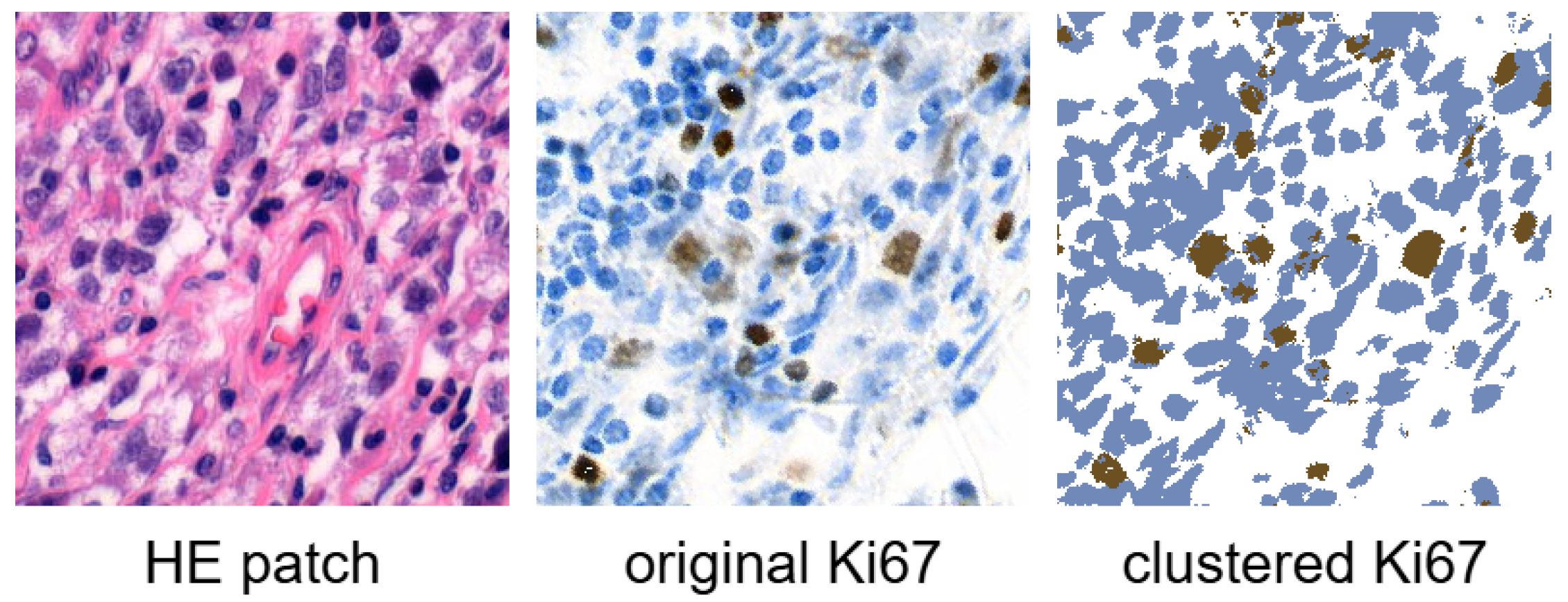
Figure 2.
Example of HE patches with Ki67 index labels from the filtered dataset, alongside their corresponding Ki67 patches.
Figure 2.
Example of HE patches with Ki67 index labels from the filtered dataset, alongside their corresponding Ki67 patches.
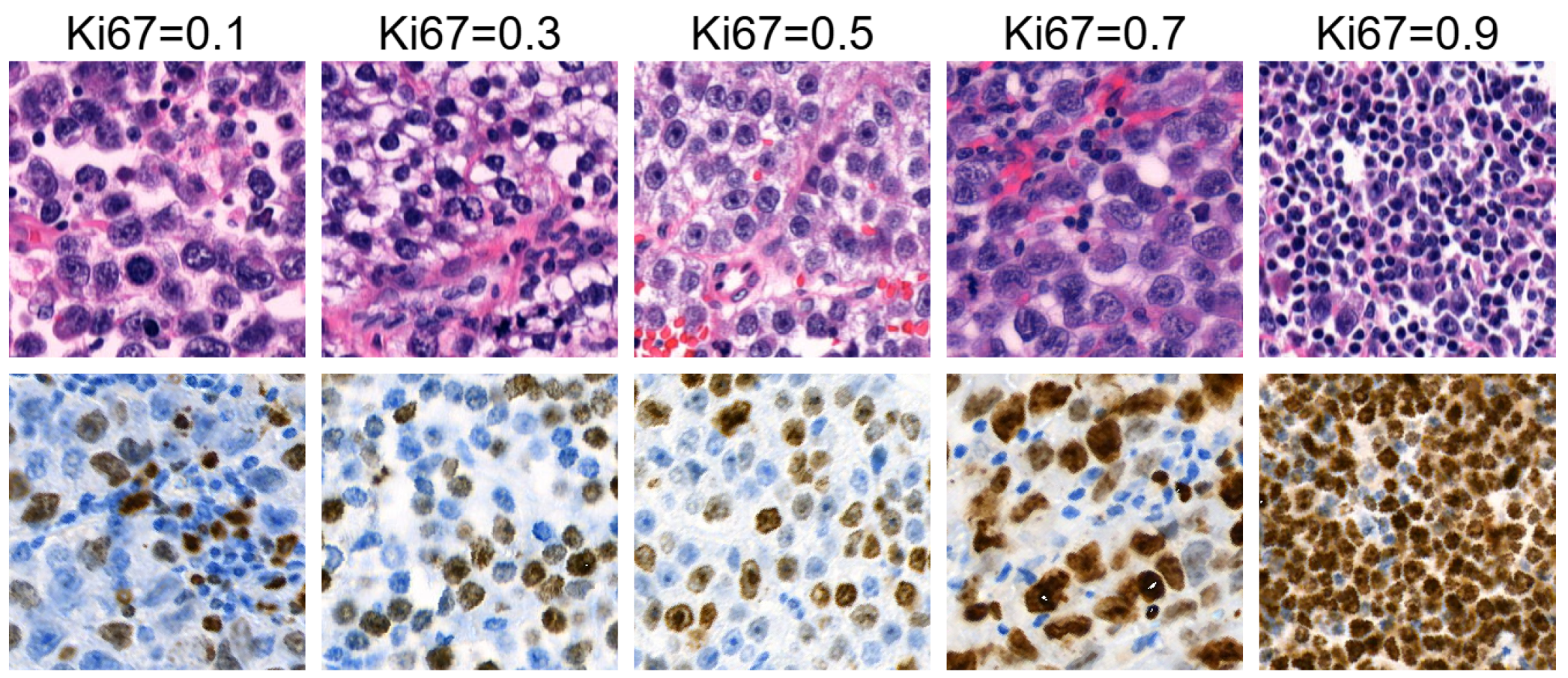
Figure 3.
Example of HE patches excluded by our filter [7].
Figure 3.
Example of HE patches excluded by our filter [7].
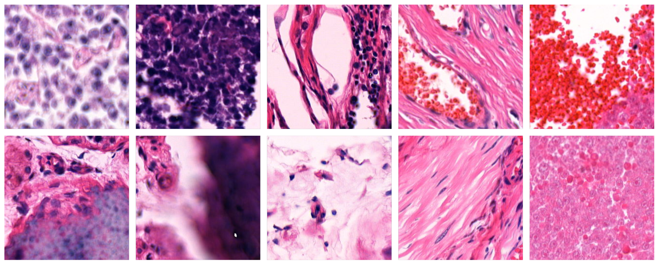
Figure 4.
Conditional GAN [7].
Figure 4.
Conditional GAN [7].
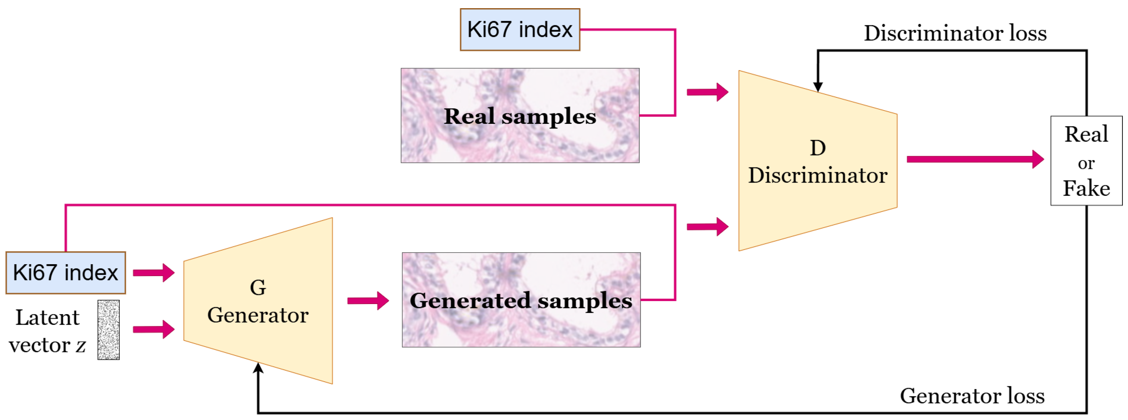
Figure 5.
Training progress in FID and PPL metrics [7]: (a) FID scores. (b) PPL scores.
Figure 5.
Training progress in FID and PPL metrics [7]: (a) FID scores. (b) PPL scores.
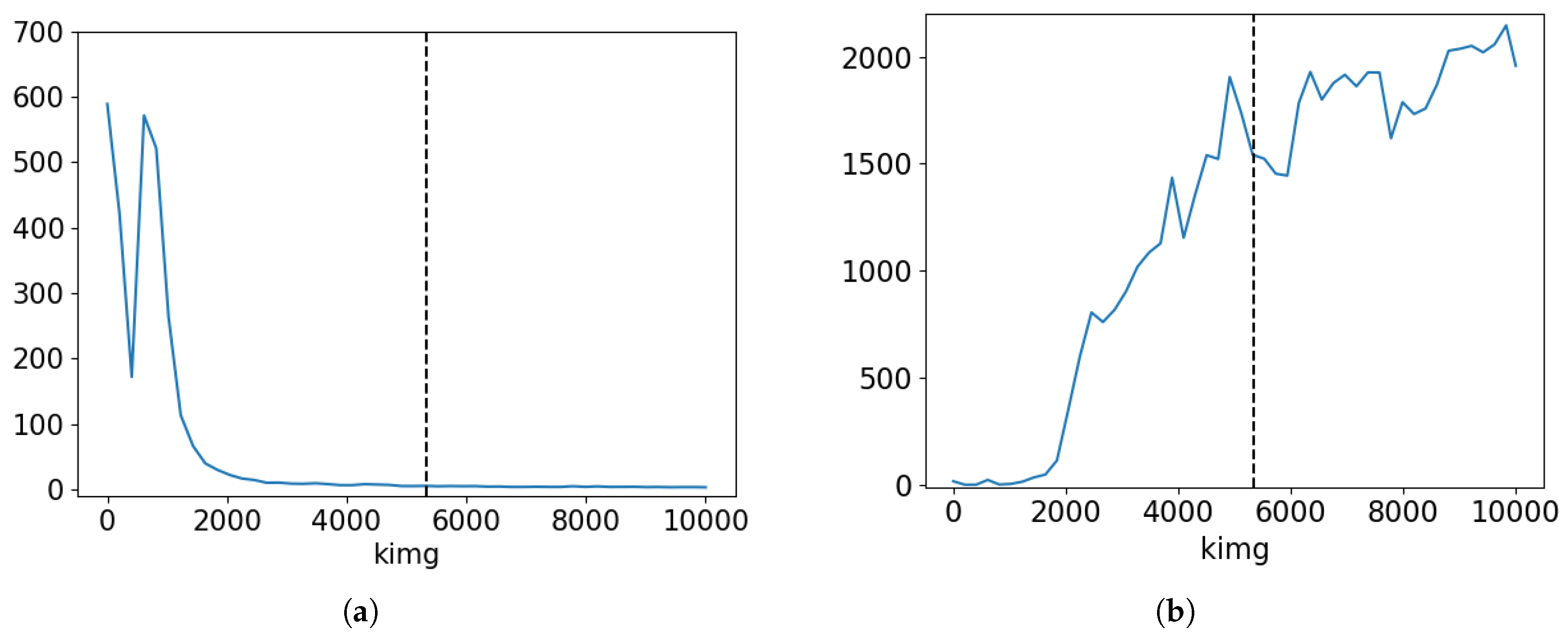
Figure 6.
Ki67 intervals.
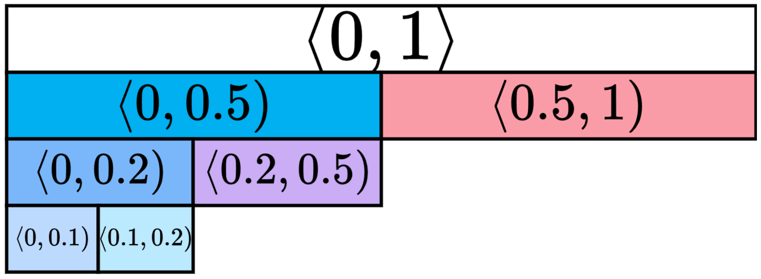
Figure 7.
The distribution of real HE-stained images across Ki67 intervals in the dataset.
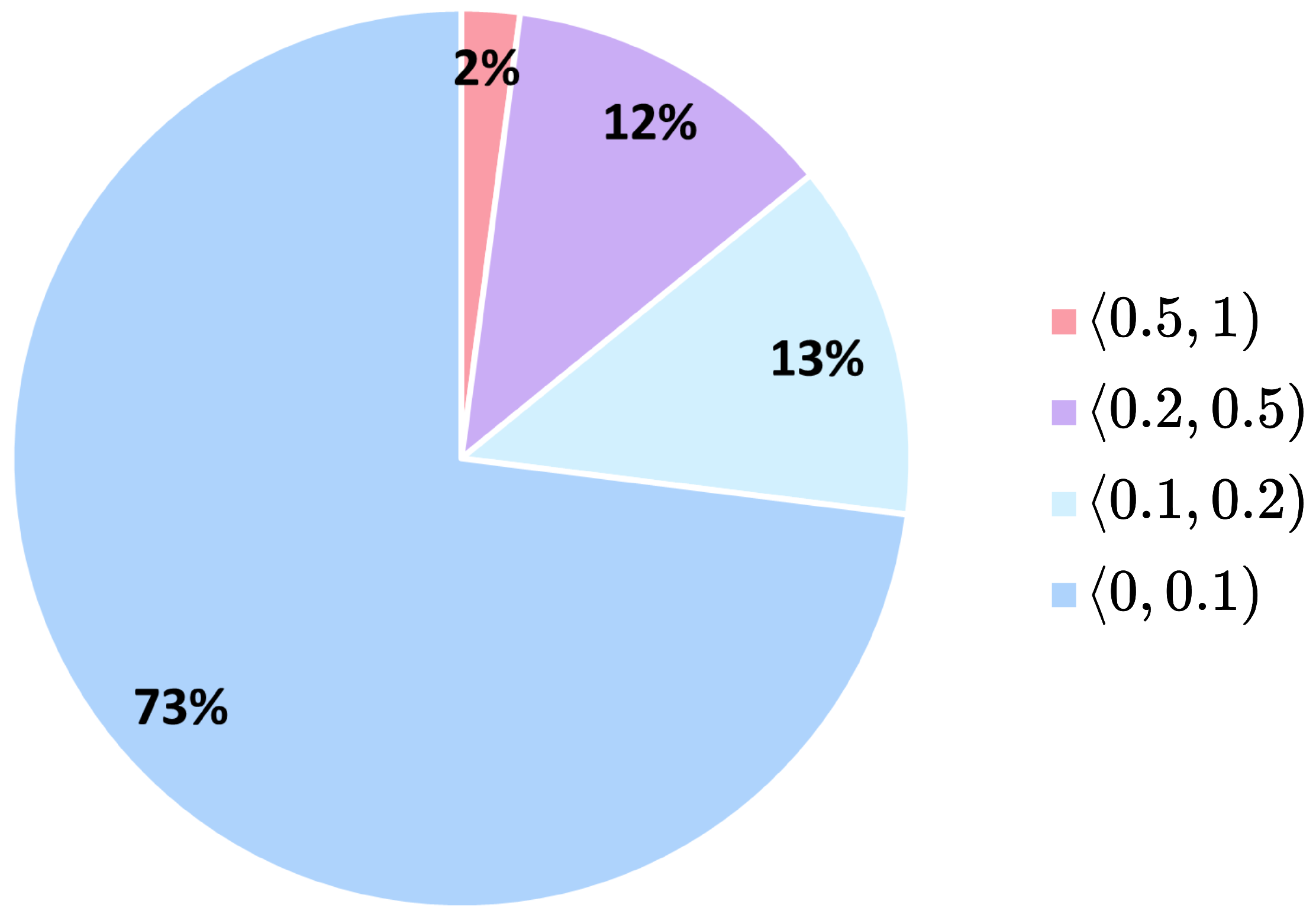
Figure 8.
The first group of sequences generated by the conditional StyleGAN model trained for 5343 kimgs.
Figure 8.
The first group of sequences generated by the conditional StyleGAN model trained for 5343 kimgs.
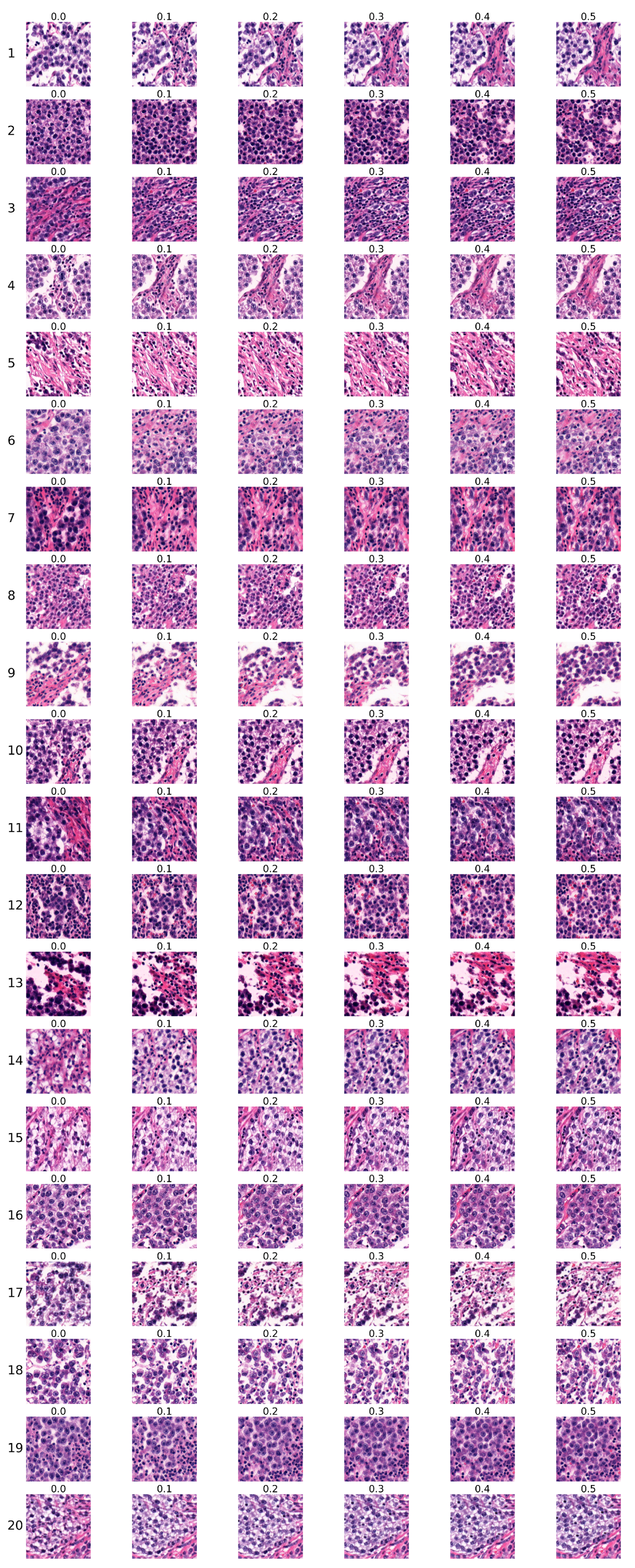
Figure 9.
The second group of sequences generated by the conditional StyleGAN model trained for 10000 kimgs.
Figure 9.
The second group of sequences generated by the conditional StyleGAN model trained for 10000 kimgs.

Table 1.
FID results on dataset vs. generator Ki67 intervals.
| generator | ||||||||
| dataset | <0.5,1> | <0,0.5) | <0.2,0.5) | <0,0.2) | <0.1,0.2) | <0,0.1) | ||
| <0.5,1> | 15.16 | 19.10 | 16.45 | 19.85 | 17.18 | 20.52 | ||
| <0,0.5) | 19.72 | 5.67 | 9.80 | 5.52 | 7.13 | 5.59 | ||
| <0.2,0.5) | 20.50 | 8.17 | 9.90 | 8.42 | 9.45 | 8.57 | ||
| <0,0.2) | 22.12 | 5.45 | 10.26 | 5.59 | 7.24 | 5.65 | ||
| <0.1,0.2) | 19.53 | 6.52 | 8.76 | 6.59 | 6.61 | 7.01 | ||
| <0,0.1) | 20.77 | 5.86 | 10.75 | 5.67 | 7.72 | 5.64 | ||
Table 2.
FHD results on dataset vs. generator Ki67 intervals.
| generator | ||||||||
| dataset | <0.5,1> | <0,0.5) | <0.2,0.5) | <0,0.2) | <0.1,0.2) | <0,0.1) | ||
| <0.5,1> | 32.41 | 43.08 | 33.39 | 45.68 | 37.62 | 47.95 | ||
| <0,0.5) | 45.40 | 10.36 | 19.85 | 10.41 | 12.95 | 10.83 | ||
| <0.2,0.5) | 35.47 | 23.42 | 20.71 | 25.70 | 22.31 | 26.67 | ||
| <0,0.2) | 44.97 | 10.49 | 21.05 | 10.45 | 13.70 | 10.77 | ||
| <0.1,0.2) | 37.01 | 15.28 | 17.56 | 16.51 | 13.07 | 17.83 | ||
| <0,0.1) | 47.78 | 11.32 | 23.86 | 11.14 | 15.31 | 11.03 | ||
Table 3.
FHD results on generator vs. generator Ki67 intervals.
| generator | ||||||||
| generator | <0.5,1> | <0,0.5) | <0.2,0.5) | <0,0.2) | <0.1,0.2) | <0,0.1) | ||
| <0.5,1> | 0.42 | 33.87 | 13.11 | 38.12 | 29.10 | 41.70 | ||
| <0,0.5) | 33.87 | 0.45 | 9.99 | 0.70 | 3.27 | 1.05 | ||
| <0.2,0.5) | 13.11 | 9.99 | 0.44 | 12.92 | 5.72 | 15.35 | ||
| <0,0.2) | 38.12 | 0.70 | 12.92 | 0.44 | 4.41 | 0.61 | ||
| <0.1,0.2) | 29.10 | 3.27 | 5.72 | 4.41 | 0.42 | 6.00 | ||
| <0,0.1) | 41.70 | 1.05 | 15.35 | 0.61 | 6.00 | 0.44 | ||
Table 4.
FHD results on dataset vs. dataset Ki67 intervals.
| dataset | ||||||||
| dataset | <0.5,1> | <0,0.5) | <0.2,0.5) | <0,0.2) | <0.1,0.2) | <0,0.1) | ||
| <0.5,1> | 0.00 | 40.95 | 31.47 | 44.38 | 32.75 | 47.80 | ||
| <0,0.5) | 40.95 | 0.00 | 12.82 | 0.30 | 6.19 | 0.87 | ||
| <0.2,0.5) | 31.47 | 12.82 | 0.00 | 16.81 | 9.43 | 19.56 | ||
| <0,0.2) | 44.38 | 0.30 | 16.81 | 0.00 | 7.72 | 0.24 | ||
| <0.1,0.2) | 32.75 | 6.19 | 9.43 | 7.72 | 0.00 | 10.58 | ||
| <0,0.1) | 47.80 | 0.87 | 19.56 | 0.24 | 10.58 | 0.00 | ||
Table 5.
PPL results on Ki67 intervals.
| <0,1> | <0.5,1> | <0,0.5) | <0.2,0.5) | <0,0.2) | <0.1,0.2) | <0,0.1) |
| 1|l|1526.11 | 1561.95 | 1549.54 | 1496.20 | 1533.52 | 1482.50 | 1559.26 |
Table 6.
Pathologist evaluation of the first group of sequences generated by the conditional StyleGAN model trained for 5343 kimgs.
Table 6.
Pathologist evaluation of the first group of sequences generated by the conditional StyleGAN model trained for 5343 kimgs.
| sequence order |
Certainly Unreal |
Rather Unreal |
Partially Real and Unreal |
Rather Real |
Certainly Real |
|---|---|---|---|---|---|
| 1 | 1 | 2 | |||
| 2 | 1 | 2 | |||
| 3 | 1 2 | ||||
| 4 | 1 2 | ||||
| 5 | 1 2 | ||||
| 6 | 2 | 1 | |||
| 7 | 1 2 | ||||
| 8 | 2 | 1 | |||
| 9 | 2 | 1 | |||
| 10 | 2 | 1 | |||
| 11 | 1 2 | ||||
| 12 | 2 | 1 | |||
| 13 | 1 2 | ||||
| 14 | 2 | 1 | |||
| 15 | 1 | 2 | |||
| 16 | 1 | 2 | |||
| 17 | 1 | 2 | |||
| 18 | 1 2 | ||||
| 19 | 2 | 1 | |||
| 20 | 1 | 2 |
Table 7.
Distances between pathologist evaluation of the first group of sequences.
| Distance | Number of sequences |
|---|---|
| 0 | 7 |
| 1 | 7 |
| 2 | 6 |
| 3 | 0 |
| 4 | 0 |
Table 8.
Summary of pathologist evaluation of the first group of sequences.
| Certainly Unreal |
Rather Unreal |
Partially Real and Unreal |
Rather Real |
Certainly Real |
|
|---|---|---|---|---|---|
| Pathologist 1 | 0 | 3 | 8 | 9 | 0 |
| Pathologist 2 | 2 | 5 | 4 | 6 | 3 |
| Pathologist 1 and 2 | 2 | 8 | 12 | 15 | 3 |
Table 9.
Pathologist evaluation of the second group of sequences generated by the conditional StyleGAN model trained for 10000 kimgs.
Table 9.
Pathologist evaluation of the second group of sequences generated by the conditional StyleGAN model trained for 10000 kimgs.
| sequence order |
Certainly Unreal |
Rather Unreal |
Partially Real and Unreal |
Rather Real |
Certainly Real |
|---|---|---|---|---|---|
| 1 | 1 2 | ||||
| 2 | 1 2 | ||||
| 3 | 1 | 2 | |||
| 4 | 2 | 1 | |||
| 5 | 1 2 | ||||
| 6 | 1 | 2 | |||
| 7 | 1 | 2 | |||
| 8 | 2 | 1 | |||
| 9 | 1 2 | ||||
| 10 | 2 | 1 | |||
| 11 | 2 | 1 | |||
| 12 | 2 | 1 | |||
| 13 | 1 | 2 | |||
| 14 | 2 | 1 | |||
| 15 | 1 | 2 | |||
| 16 | 1 | 2 | |||
| 17 | 1 | 2 | |||
| 18 | 1 | 2 | |||
| 19 | 2 | 1 | |||
| 20 | 2 | 1 |
Table 10.
Distances between pathologist evaluation of the second group of sequences.
| Distance | Number of sequences |
|---|---|
| 0 | 4 |
| 1 | 7 |
| 2 | 6 |
| 3 | 2 |
| 4 | 1 |
Table 11.
Summary of pathologist evaluation of the second group of sequences.
| Certainly Unreal |
Rather Unreal |
Partially Real and Unreal |
Rather Real |
Certainly Real |
|
|---|---|---|---|---|---|
| Pathologist 1 | 1 | 6 | 3 | 8 | 2 |
| Pathologist 2 | 3 | 7 | 3 | 2 | 5 |
| Pathologist 1 and 2 | 4 | 13 | 6 | 10 | 7 |
Disclaimer/Publisher’s Note: The statements, opinions and data contained in all publications are solely those of the individual author(s) and contributor(s) and not of MDPI and/or the editor(s). MDPI and/or the editor(s) disclaim responsibility for any injury to people or property resulting from any ideas, methods, instructions or products referred to in the content. |
© 2025 by the authors. Licensee MDPI, Basel, Switzerland. This article is an open access article distributed under the terms and conditions of the Creative Commons Attribution (CC BY) license (http://creativecommons.org/licenses/by/4.0/).
Copyright: This open access article is published under a Creative Commons CC BY 4.0 license, which permit the free download, distribution, and reuse, provided that the author and preprint are cited in any reuse.


