

Submitted:
10 March 2025
Posted:
12 March 2025
You are already at the latest version
Abstract
The present work provides a framework for the comprehensive assessment of energy harvesting resources in buildings, encompassing environmental, anthropogenic and recyclable sources. A review of resources and state-of-the-art energy harvesting technologies is presented including an outlook on the future theoretical limitations of their performance. The assessment framework is applied to a case-study commercial building located in Toronto, Ontario, Canada. Available resources are categorized into 3 orders of magnitude with respect to achievable power generation, with solar and wind in the first tier, elevator potential and fitness centres in the second tier, and sources including vibrations, occupant traffic and thermoelectric conversion in the third. Situated in a mid-rise context, the total annual resource magnitude is found to be 8 times greater than the building demand. However, only an overall 10% of the available resource is converted with the harvesting applications and efficiencies considered, resulting in a net energy deficit. It is shown that with maximum theoretical efficiencies, the conversion rate can reach 30% resulting in 151% surplus electrical generation for the building in question.
Keywords:
energy harvesting
; buildings
; microgrids
; photovoltaics
; wind turbines
; piezoelectric
; thermoelectric
1. Introduction
Building level microgrids have become a topic of increasing relevance for the integration of onsite energy sources in the interest of energy resilience and load management [1], [2]. The growing prevalence of native direct current (DC) devices, coupled with concerns for efficiency and power quality have led to isolated power distribution architectures involving DC or otherwise asynchronous current [3], [4]. The presence of an isolated microgrid at the building level may enhance the feasibility of small-scale generation from energy harvesting sources which are traditionally considered unworthy for integration with the synchronous utility grid. Energy harvesting from alternative sources enhances generation diversity, enabling levels of autonomy and resilience that are unattainable when solar, storage and utility supply are the only available resources.
Energy harvesting options in buildings are frequently assessed in the literature with detailed focus on a given resource, technology, or application. Few studies however - with the exception of Matiko et al. [5] - have endeavoured to develop a comprehensive resource assessment, which is the goal of the present work. The following sections provide a review and quantification framework for the available energy harvesting resources in buildings. Current and future technology limitations are discussed, and the framework is applied to a high-performance commercial building model to characterize the various resources.
This work does not intend to provide an exhaustive review of specific energy conversion technologies, but rather to provide a summary of available energy resources and pertinent technologies, with speculation about the future potential for application in buildings. The resources are limited to those which are readily converted into the electrical domain. Energy sources harvestable in the thermal domain will be addressed in a follow-up work.
1. Energy Resources in Buildings
At a high level, a building may be considered an open thermodynamic system, which exchanges energy with its surroundings via three main mechanisms: the exterior environment, occupants, and concentrated utility inputs. This concept is presented in Figure 1, where the building system boundary may be considered to include exterior surfaces and a finite surrounding air volume.
In this depiction, Ein comprises energy added to the system from environmental sources and utility inputs. Wint denotes the internal work done in the system, which is equivalent to the total energy consumed for end-use functions such as lighting, space conditioning, etc. This can also be considered the traditional energy demand of the building. Eint represents the energy generated internally from building occupants, as well as internal dissipation of environmental energies and utility sources in the execution of useful work. The latter two of these sources can cumulatively be denoted Erec, or recyclable energy. Eout represents the balance of energy that is dissipated to the surroundings. In this representation, the internal energy of the building system cannot be easily described by a single state function, which complicates any effort to produce a steady-state energy balance. However, the thermodynamic components described can be broken down as follows in Equations 1 through 3,
With reference to this framework, energy harvesting can be employed to maximize the proportion of Eenv and Eint which can be utilized for useful work (Wint) such that Eutil and Eout can be minimized. Of course useful work should not be considered a harvestable resource, as this action would increase the necessary input energy to overcome harvesting inefficiencies, ultimately affecting demand negatively. The generalized components of Ein and Eint can be further broken down into specific resource categories, as depicted in Figure 2.
With the specific resources identified, the total energy generated from energy harvesting, Egen, may be approximated by Equation 4,
Solar
The solar energy resource is comprised of electromagnetic radiation in the spectrum of 300-1100 nm. The magnitude of this resource is best evaluated on an annual interval due to seasonal and diurnal variability. A sun path diagram for the case study location of Toronto is presented in Figure 3, which indicates the variation in relative position and duration of sun exposure over the course of a year.
The magnitude and variability of the solar resource at a given location depends predominantly on latitude, sky clearness and the orientation of the collection surface, commonly denoted the plane of array. The available resource on a given collection surface can be defined as the sum of the direct beam irradiance, diffuse irradiance and ground reflected irradiance, in accordance with Equation 5,
In this simplified case the direct beam component may be derived as a function of the local direct normal irradiance (DNI) and angle of incidence (AOI) between the collection surface and the sun rays as described by Equation 6,
The ground reflected irradiance component can be described as a function of the local albedo, or solar reflectance in accordance with Equation 8,
In urban environments, the solar resource is variably affected by shading from neighbouring buildings and additional structures. In this case, a shading factor may be applied to the surface area in question, or ideally a detailed shading analysis may be conducted based on exact local and neighboring geometries.
Artificial Light
The other radiative resource in buildings is artificial light which is generally designed in reference to desired illuminance or lux, a function of the human eye’s response to visible spectrum radiation. Lumens can be translated to equivalent watts of radiation with reference to the photopic curve, which defines the human eye response spectrum. With reference to the photopic conversion, Dai et al. [11] show achievable luminous efficacy from high-efficiency LED lighting in the range of 400 lumens per watt provided that constraints relating to colour temperature are upheld. Taking the inverse of this luminous efficacy term allows an approximation of the available radiant energy in a space dependent upon the lighting intensity. For example, in an office space with design lighting intensity of 400 lux at desk level, the available radiant energy, presuming Dai’s high efficiency lighting would be 1 watt/m2. Non-LED lighting technologies exhibit lower luminous efficacy, which indicates greater available energy. However, much of the radiant energy of an incandescent bulb for example, is emitted in the infrared spectrum which is not readily accessible for electrical conversion. By contrast, the spectrum of high efficiency lighting is inherently concentrated within the accessible range of common photovoltaic devices.
Wind
The wind energy resource is a form of kinetic energy associated with the motion of air in accordance with global thermal gradients and weather patterns. Like the solar resource, wind energy experiences seasonal variation with larger magnitudes typically observed in winter seasons due to larger temperature gradients in atmospheric air masses. A given location may experience a prevailing wind direction from which most of the wind resource acts, however wind can be expected to act from all directions throughout the course of a year, especially in urban environments where neighboring obstructions have dominant influence. A wind rose diagram for the case study location of Toronto is presented in Figure 4.
The available power in a wind resource described on a per unit area basis by Equation 9,
Wind velocity can be further altered by interaction with building geometries. Initially, a large portion of the kinetic energy will be translated into static pressure, ultimately dissipating as vibration and mechanical strain in the building structure. In the laminar domain, flow affects include deceleration due to boundary layer friction at the building surface and acceleration around exterior corners. The latter has been described by You et al. as a function of the flow velocity ratio [14]. Flow interactions with geometric objects can also produce a transition to the turbulent domain. Turbulence is characterized by disordered kinetic energy, having inherently limited harvesting potential. In urban environments upstream flows may be largely turbulent in advance of interactions with a given building structure because of neighboring buildings. These affects interact differently depending on the specific local geometry of the building to influence the effective wind speed at any given unit area around the building exterior.
The static pressure component of wind energy has value in buildings in its capacity to drive natural ventilation. Ventilation system energy demand may be reduced if ventilation is enabled via wind pressure gradients. There are generally seasonal constraints to this approach in cold climates, however these may be addressed with passive energy recovery ventilation approaches, as proposed in the literature [15], [16].
For the purposes of available energy assessment, the total magnitude of the wind resource available at a building can be considered with reference to Equation 9. The average wind speed upstream of a building is approximated based on the local weather data and height compensation via the power law. The relevant catchment area can be defined instantaneously as the cross-sectional area of a building in the plane normal to the instantaneous direction of wind speed. The resultant power calculation can be integrated over a typical annual interval to determine the total annual resource. The geometrical relations of the instantaneous catchment area are represented as a function of wind direction in Figure 5.
The width of the catchment area is defined by Equation 12, as a function of the wind direction,
As with the solar resource, this fundamental assessment will often be implicated due to flow effects from upstream geometries. These effects may be accounted for with a simple modification to the catchment area, however computational fluid dynamics (CFD) modelling should be employed for most accurate assessments of the interactions with urban environments and neighbouring geometry. The monthly wind resource density at a height of 20 m, based on Toronto’s Billy Bishop Airport weather data is presented in Figure 6, in contrast to the monthly solar resource. Note that the unit area referenced in Figure 6 is not constant for the two resources; the solar resource represents the sum of 5 cardinal building surfaces, while the wind resource is quantified with respect to the instantaneous catchment area, described above.
Vibration
Structural
In locations prone to seismic activity, ground vibrations may occur periodically in large magnitude. However, in the absence of seismic events smaller magnitude ground vibrations are often present due to anthropogenic activity in the surroundings including vehicle traffic and construction [17]. Buildings may also experience vibrations induced from internal machinery and HVAC equipment, as well as the motion of occupants. In the case of tall, slender buildings wind induced oscillation are also present.
Energy in vibrations can be described as a combination of kinetic and elastic energy forms oscillating sinusoidally at phase angles of 180° with respect to each other. In most cases, the kinetic energy of ambient ground vibrations is too small to be observed by human sensory but may be observed with accelerometers. The elastic energy manifests as elastic strain in the structural materials of the building.
The magnitude of the vibration resource at a given location is difficult to determine from readily available data sources such as weather files. However, extensive work exists in the literature on the understanding and attenuation of structural dynamics. Valera et al. have shown that for a medium rise building, the largest contributors to structural vibrations were ground motions from vehicle traffic and internal vibrations from air-conditioning equipment, at peak frequencies 8 and 29 Hz, respectively. Roundy et al. [18] note available energy density in the range of 50-250 μW/cm3 from common ambient vibrations in buildings with reference the volume of a harvesting device. Priya [19] defines the maximum power available in a vibrating mechanical system in accordance with Equation 13, which stems from the original analysis provided by Williams and Yates [20],
For a structurally integrated energy harvesting, the effective seismic mass can be considered the modal mass of the relevant structural body’s experiencing vibration. Modal mass is defined as the fraction of mass which is effectively resonant - about 25% of total mass for beams with fixed supports. The damping ratio in building structures as described by Valera is quite low at around 2% for concrete. Frequency and acceleration magnitudes describe the excitation.
In cases where vibrations are present in large magnitudes from either seismic or wind loading conditions, buildings will often employ tuned-mass dampers as attenuation mechanisms. In order to function successfully the damping devices are required to dissipate large amount of energy as heat, which may be otherwise available for energy harvesting, as presented by Petrini et al. [21].
Equipment
Machine-based vibrations are a result of internal rotating unbalance. In the literature, these types of vibrations are well documented from the perspective of vibration damping, however there is limited work aimed at deriving the total available power. With reference to fundamental dynamics, the forcing function of a rotating unbalance is a function of the rotating mass and eccentricity internal to the machine [22]. These details are of course difficult to acquire for any given machine, thus the key interest to the present work is the ability to derive the total available power with reference to readily available characterization data, such as the machine’s total mass, acceleration amplitude, and frequency of vibration. Many articles considering energy harvesting from machine vibrations, consider only small seismic masses which do not affect the excitation vibration, and are thus limited in their harvesting potential. Wang and Inman [23] provide a review of approaches to vibration damping which endeavour to achieve optimal results in the contexts of both energy harvesting and vibration suppression, indicating the trade-offs present between the two objectives. Bulsara et al. [24] show that losses for experimentally applied unbalances can exceed 50% of balanced energy consumption for a given rotating speed and relate the power losses to unbalance at an average of 0.11 W/g-mm. However, rotational unbalance is generally considered an undesirable quality from the machine design perspective, and thus the results of Bulsara can be interpreted as an extreme representation.
Two methods exist to approximate the available energy. The first is a top-down approach which considers the energy of vibration as a loss mechanism of the input energy and thus relates to the efficiency of the machine. The second is a bottom-up derivation based on the vibration dynamics. As the model presented by Williams and Yates assumes the excitation power to be infinite, it cannot apply.
Assuming damping effects are negligible, a vibrating machine can be considered as a simple spring-mass system under a periodic excitation force. The energy of a given cycle can be equated to the peak kinetic energy as described by Equation 14,
The power dissipated in the system can then be described as a function of the forcing frequency, f, in Hz, per Equation 15,
In the literature, vibrations are typically characterized by peak acceleration, amax, and frequency, f. As velocity can be defined as the integral of acceleration over time, and the acceleration can be characterized as a sinusoidal function, the relationship between peak velocity, max, and peak acceleration can be described by Equation 16,
Substituting Equations 14 and 16 with Equation 15 yields the following derivation for available power in a spring mass system under forced vibration:
Applying the above formula to an example from Priya involving a 5 HP machine with peak acceleration of 10 m/s2, frequency of 70 Hz, and assumed mass of 2000 kgs, produces 36 W of available power, or roughly 1% of the rated machine power. In the interest of simplifying this analysis it is assumed going forward that the available power from relatively well-balanced vibrating machinery is on the order of 1% of the machines total demand.
Potential
Potential energy is a particularly relevant resource in tall buildings, due to large variations in height. The two mechanisms explored herein are micro hydro and elevator regeneration.
Micro Hydro
The potential energy available from stormwater collected on a building’s rooftop can be approximated based on gravitational potential in accordance with Equation 18,
In many cases, the more significant hydropower resource in a building may be greywater, which is characterized as wastewater from domestic use which is free of solid organic waste. The difficulty with this approach in many North American buildings is the lack of separation of greywater from blackwater in plumbing systems. McNabola and Corcoran have examined the potential of micro hydro at the municipal scale, from both policy [25] and technical [26] perspectives. Their analyses focused on deployment of microhydro facilities in place of flow regulation valves commonly utilized to control downstream pressure, ultimately showing that in a case study of Dublin, Ireland, microhydro could produce up to 7.5 GWh/yr from roughly 1 MW of installed capacity. In the building context, Santillan [27] presents a detailed analysis of the potential and limitations of hydropower in a residential high-rise incorporating both stormwater and grey water drainage. In this work, Santillan shows that roughly 75% of water use in a residential setting ends-up as grey wastewater. Based on the presented data, it can be assumed that in a commercial context, the proportion is closer to 50%.
In Canadian residential settings annual water consumption is on the order of 220 L/pp/day [28] while in commercial settings it has been characterized according to floor area at roughly 55 L/ft2yr when cooling tower consumption is omitted [29]. The resultant total annual consumption volume can be applied in Equation 18 to estimate the annual resource, where the relevant height value is the midpoint of the building which accounts for the averaging of gravitational potential of flows evenly distributed throughout a building.
Elevators
Energy harvesting from elevator motion works akin to the concept of regenerative braking in electric vehicles. When the potential, or momentum of a mass is driving its motion, the powertrain can be switched into reverse such that the driving motor works as a generator and the electromotive resistance in its windings provides a braking force to the mass in motion. This resource is of particular interest due to the prevalence of this regenerative braking capability in modern elevators, which is often forgone in design due to the complexity of integration with building power systems.
A detailed study of the available energy from energy regeneration was conducted by Nobile et al. [30], showing that the total recoverable energy for a single elevator trip can exceed 50% of the motor input energy after factoring mechanical and motor losses. However, the recoverable energy also varies depending on the number of passengers, direction of travel, and distance of travel. Nobile et al. categorize elevator trips into 4 types according to the ratio of passenger weight to counterweight and direction of travel. Generally, energy is harvestable only when the descending mass exceeds the ascending mass. An annual simulation of harvested energy based on audited elevator usage data from a 6-story condominium building shows that recovered energy equates to roughly 20% of the total input energy for the elevator on an annual basis. The authors note that this value may vary with usage patterns.
Without detailed traffic data for a building in question, it is considered sufficient to extrapolate this 20% recovery model to estimate annual resource based on the annual elevator demand, which can be derived from a building energy model. Detailed model derivations for elevator energy consumption that might be adapted for finer analysis in future work are presented by Tukia et al. in [31] and [32]. As a rule of thumb, elevators can be expected to account for 3-8% of energy consumption in buildings [33], with dependence on building height, occupant density and travel frequency.
Occupants
Occupants dissipate energy into a building in many forms, including kinetic, acoustic as well as sensible and latent heat. Of interest in the present work is the kinetic energy imparted by occupants into the building, in the forms of exercise and traffic across doors and floors.
Fitness
The energy exerted by humans during indoor cardiovascular exercise is typically dissipated via friction and heat in the context of stationary bikes, elliptical and rowing machines. A detailed review of the energy available from a variety of human powered fitness machines is given by Chalermthai et al [34]. The results of which are summarized below in Table 2.
Annual generation profiles from the various machines may be derived akin to the load models employed by building energy simulation tools such as EnergyPlus, where the active power is extrapolated over time according to an activity schedule. This approach would be most effective in a commercial gym where occupancy insights are available. Over an annual scale, simplifying assumptions can also be made with regards to the number of building occupants and average hours spent exercising in the building’s gym per week.
Doors
A physics-based analysis of the energy generating potential of swing and revolving doors is given by Partridge & Bucknall [35] who show that the generation potential is a function of door geometry, mass, and mechanical losses due to damping and hardware friction. Ultimately a generalized metric is provided indicating that average revolving doors may produce up to 40 J of energy per person, while swing doors have less available at closer to 10 J.
Gilani et al. [36] produced a lightweight prototype of an energy harvesting revolving door and observed average energy generation of 16 J per push. It is expected that the lower output relates to the limited mass of the door in comparison to the physics-based analysis provided by Partridge and Bucknall. Gilani et al. applied their results to a case study involving a busy mall application where it was theorized the door would rotate a maximum of 38,000 times per day for annual energy generation of 61 kWh/yr.
Extrapolating the per revolution energy data to annual generation profiles generally follows the same method of the fitness machines where a typical traffic schedule is implemented at each door in question. On the annual scale, the available resource can be predicted in accordance with an average number of revolutions or openings per day in accordance with the method presented by Gilani.
Walking Motion
During human walking motion peak forces transferred to the a floor are described by Puscasu et al. [37] as roughly 20-30% greater than body weight. In their analysis, Puscasu et al. relate this to the deflection observed in a floor tile to determine the mechanical energy transferred per step, which they show is on the order of 1 J/step for average body weight of 76 kg and 1-3 mm deflection in the floor tile. These data points can be extrapolated to determine the total available energy due to walking motion as a function of the space occupancy and steps per hour per occupant. Clemes et al. [38] have shown that the mean step count for office workers during a workday is on the order of 4000 steps, which can be translated to 500 steps per hour assuming an 8-hour work day. With these data points the available walking resource can be extrapolated on the order of 500 J/h, occupant or roughly 1.1 Wh per occupant per day.
Thermal
Thermal energy is a significant resource in buildings. In Toronto’s climate, space and water heating comprise up to 80% of residential energy demand [39]. For waste thermal energy to be converted into useful work there must be a gradient present, or a source of heat flow. The fundamental limitation of useful work that can be derived from two thermal reservoirs at different temperatures is described by the Carnot efficiency, per Equation 20,
The thermal resources that exist in buildings are generally considered components of end-use functions. For example, the heat flow across a building envelope should be minimized rather than harvested, and the heat delivered to, or removed from a space should be unhindered as to maximize the efficiency of delivery. However, thermal energy that is purposely expelled from the building is a form of energy loss that is considered a desirable resource for energy harvesting.
For waste heat applications, consideration must be given to the annual variation in thermal gradient associated with instantaneous outdoor temperatures. On an annual scale we can relate the total available resource to the energy that is expelled by the ventilation system, which relates to the energy recovered by the ventilation system according to the system heat/energy recovery efficiency. There is also a resource present in the heat that is expelled by a building’s cooling system, provided that efforts to harvest this particular resource do not interfere with the rate of expulsion. These two resources are described by Equations 22 and 23,
2. Energy Harvesting Technologies
The following sections will describe the state-of-the-art technologies available today for converting the energy resources described into the electrical domain.
Photovoltaics
The photovoltaic effect is a property of semiconductor materials and alloys which enables the production of electric current in response to absorption of light. This process relates to the bonding energy of the valence electrons in the given material, described as the band gap energy. As photons are absorbed by the material with energy greater than the band gap, electrons are displaced from the valence band of the material into the conduction band. Photovoltaic cells employ doped materials in a p-n junction to enable the efficient collection of the displaced electrons to provide current to an exterior circuit.
Due to the nature of this effect, the total conversion efficiency is a function of a given material’s band gap energy. When a photon with energy below the band gap is absorbed, no current can be produced, while a photon with energy greater than the band gap produces current but loses its excess energy to heat. The net response of a material at this level can be quantified by the quantum efficiency (QE), which is a function of photon wavelength. Mass-market photovoltaic devices are typically comprised of single-junction silicon cells which provide a relatively broad match to the terrestrial solar radiation spectrum resulting in module level efficiencies around 20%. One of the key areas of interest in photovoltaic development is the production of tandem junction cells, which utilize multiple layers of semiconductors with complimentary band gaps, such that a broader range of the incoming solar spectrum can be more efficiently collected. This concept in depicted in Figure 7 [40].
The external quantum efficiency (EQE) describes the ratio of electrons excited to photons absorbed over the range of available solar spectra. However, EQE does not account for the thermal losses resulting from photon energies above the band gap. The ultimate limit to efficiency with this relation considered has been presented in the Shockley-Queisser limit [41], which defines the maximum achievable conversion efficiency for a single junction solar cell, shown to maximize around 33.8% [42]. Following Shockley’s approach, the theoretical efficiency limitation for an infinite junction tandem cell has been subsequently defined by Vos as 68.2% [43]. Alharbi and Kais [44] provide a thorough review of the prospects in approaching these theoretical limits with feasible technologies.
PV efficiency limits are generally defined at standard test conditions (STC) involving AM1.5 irradiance spectrum and 25°C. In practice cell efficiency is further limited by actual operating temperature, incident irradiance spectra, and manufacturing limitations, among other factors.
Theoretical efficiency can be increased by enhancing the intensity of the incident radiation, as is the approach taken by concentrated PV (CPV) cells. High levels of concentration have been shown by Vos to increase the theoretical efficiency above 40% for single junction cells, however this technology has generally not proven successful in practice due to combatting thermal issues which reduce the practical efficiency and risk cell damage. CPV also lacks effectiveness with diffuse and reflected radiation, which can represent a significant portion of the available resource in cloudy climates.
Additional approaches exist in practice that enable enhanced utilization of a given surface for light collection. With these methods, efficiency is not improved, but net output gains per unit surface area are achieved by increasing total access to light. Noteworthy technologies include single and double axis tracking systems which control the orientation of collection surfaces throughout the day to minimize the AOI, resulting in achievable additional production of 25% and 45%, respectively, dependent on location [45]. Alternatively bifacial cells which are rapidly gaining industry adoption, enable light collection on both the front and back side of a cell enabling collection of reflected, diffuse, and artificial light that may be present on the side of the cell which faces away from direct radiation. This technology has been shown to enable annual energy gains on the order of 25% in traditional array geometries [46].
When considering building integrated application for photovoltaics, the most common application is to mount traditional PV panels in a fixed tilt orientation on a roof. However, innovative products are in development that integrate photovoltaic technology into traditional cladding systems. This concept of cladding integrated PV trends towards enabling combined BIPV/T systems which harvest waste heat from PV collectors to serve a buildings thermal demand [47]. In addition, a few advanced technologies exist for integrating PV properties into glass, to enable energy production without compromising visible transmittance. Of course, these applications are limited in the achievable efficiency given their transparent nature, with published results in the range of 3.6% [48].
Turbines
Wind harvesting turbines can be generally categorized into two main types: horizontal axis (HAWT) and vertical axis (VAWT). Horizontal axis machines comprise the bulk of utility scale wind farms due to their relatively high efficiency [49]. The blades of a HAWT rotate in a vertical plane and thus must be controlled, either actively or passively, to point into the wind stream in order to extract maximum power.
Vertical axis turbines utilize blades which rotate in the horizontal plane. Because of this feature, VAWTs can extract power from all wind directions without orientation control, lending to suitability in locations with a high degree of variability in the wind resource. There are two main types of VAWTs; Savonius and Darrieus, which operate on drag and lift forces, respectively [50]. Darrieus, or lift based VAWTs generally have a higher achievable efficiency, however, are unable to self-start due to their symmetry, thus requiring input energy to initiate rotation. Savonius, or drag-based VAWTs are self-starting and require the least amount of control, yet exhibit the lowest efficiency of the surveyed machines [51]. Combined VAWT designs are commonly deployed such that the Savonius component provides the self-starting torque and the Darrieus component enables higher efficiency operation at higher wind speeds. Each design may also be modified with a helical twist along its axis which acts to reduce backside drag in effort to increase the achievable Power Coefficient, (Cp). The various models are depicted in Figure 8 [52].
A noteworthy difference between drag and lift type turbines is their effective tip-speed ratio, and resultant machine RPMs. Drag-based turbines are limited to a tip speed ratio of 1 and thus generally require gearboxes to amplify the rotational velocity to a compatible rate with the generator being utilized. For lift-based turbines higher tip speed ratios can be achieved [53], which may enable direct motor drive applications. The addition of a gearing system to the power train will generally introduce losses on the order of 5%, which may be worthwhile dependent on the base turbine rotational dynamics. Motor generator typologies will be briefly discussed in Section 3.5. In efforts to harvest consistently low wind speed crossflow VAWT designs have been suggested [54] and shown to exhibit the highest achievable power coefficient of existing turbines at tip speed ratios below 0.5. The performance benefit of this typology however has not been proven in practice [55].
Available wind power can be derived from a laminar flow in accordance with Equation 24, which builds on Equation 9, with the addition of area, power coefficient and efficiency terms,
Wind turbine power coefficients vary with wind speed, typically maximized at rated wind speed and decreasing at higher speeds due to stability limitations. The maximum Cp that can be achieved in a wind turbine is ultimately limited by Betz law, which applies to fluid flow in an open system, and works out to 16/27 or 59.3% of the total available energy [56]. This limitation follows from the notion that 100% efficiency would necessitate downstream air molecules to be motionless, meaning additional molecules would be prevented from flowing through the turbine, and would flow around it instead. Common Cps for the turbine types describes are presented in Table 3.
Given the capacity of building geometry to affect wind velocity as described in Section 2.2, many researchers have proposed building integrated wind turbine designs which leverage building geometry to accelerate flows strategically across a turbine to increase yield. This concept of building integrated wind is well demonstrated in [57] and [58] where wind turbines are positioned horizontally between neighbouring towers as well as vertically between stories of a given building. Both authors note the importance of optimal building geometry in order to maximize the effective velocity ratio acting to accelerate incoming flows. Hassanli et al. [59] proposed a double skin façade system designed for the purposes of wind energy harvesting, ultimately noting that turbulence is reduced inside the façade cavity and average speed is increased.
Recently, interest has developed towards resonant wind harvesting devices, described as bladeless turbines. These machines employ vertical members hinged near the base to enable single degree of freedom oscillations induced via vortex shedding. The resultant oscillations may be converted into electricity via piezoelectric materials or coupling with a permanent magnet alternator, as proposed by Villarreal [60].
In hydro applications, flows are contained closed systems where Betz law does not apply, so higher Cps can be achieved. Jawahar & Michael [61] present efficiencies ranging from 60-91% for turbines relevant to micro hydro application. Santillan concludes that the Pelton type, which operates at low speeds and high pressure, is the most appropriate selection for building application. Crossflow turbines may also be well suited to certain buildings depending on the characteristics of the given resource. Binama et al. [62] note the potential benefits of simple pump geometries deployed as turbines, which are shown to achieve efficiencies up to 80% in a well-tuned system with dramatically lower capital cost than their more sophisticated counterparts.
Piezoelectric Materials
The piezoelectric effect is the accumulation of electric charge in a material in response to mechanical stress. Piezoelectric materials are inherently dielectric and anisotropic with asymmetric dipole distributions in their crystal lattice. These properties lend to electric polarization in response to distortion in the crystal lattice of a material from an applied stress. This dynamic is described by the electro-mechanical coupling equations, presented in Equations 25 and 26, which relate the mechanical and dielectric responses of a material via the piezoelectric effect;
The magnitude of energy transduction between mechanical and electrical forms in a piezoelectric material depends on the material’s coupling coefficient; k2 defined generally as the ratio of electrical energy stored in the material to mechanical energy input. The coupling coefficient can be related to the basic physical properties of the material in accordance with Equation 27,
Covaci & Gontean [60] note that a high degree of system coupling can be elusive at low vibration frequencies due to the difficulty of enabling low resonant frequencies in a harvesting device. Generally piezoelectric ceramics have higher resonant frequencies, while piezoelectric polymers can achieve lower frequencies. This would indicate that polymer materials are better suited to building applications given the lower frequency vibrations that are generally present [18], [16].
In a building, numerous applications can be theorized for piezoelectric energy harvesting. Many researchers have explored the alluring opportunity of integrating piezoelectric materials into building structures. As described by Chen et al. [67] compatibility between cement and piezoelectric treatments has been demonstrated. Chen at al. summarize several treatment methods and additives explored in the literature to create a piezoelectric effect in concrete mixtures. A common method of applying piezoelectric materials for vibration damping is the shunt damping approach, which described by Moheimani & Fleming [68] as the structural bonding of a piezoelectric transducer to a flexible material with external electrical impedance or load. This represents a promising approach for integration into non-concrete building structures which align well with impactful industry goals of reduction in lifecycle carbon.
At the microscale, the bimorph architecture is a common device typology where piezoelectric materials are applied to either side of a cantilevered beam under vibration. Recent work most commonly focusses on bimorph harvesters applied to base vibrations with a small proof mass to excite the bimorph at its natural frequency ([69]; [70]). However, the bimorph architecture can also be applied in shunt damping applications. A detailed electrical-mechanical model for a bimorph shunt damper is presented by Liao & Sodano [71] to inform optimal placement of piezoelectric patches and resultant dynamic response of cantilevered beams.
In the context of piezoelectric roadways which can be applied in building parking garages and neighbouring parking lots, Wang et al. [72] report annual energy output of 188 kWh/lane/mile, in accordance with the model results presented by Zhang et al. [73]. Zhang’s results have shown that the instantaneous power output from a single piezoelectric transducer embedded in a roadway is proportional to vehicle velocity, with reported output of 47 mW under a 4-wheel load at 30 m/s. Guo & Lu [74] contrarily report results from literature as well as their own analysis which indicate outputs of 200 and 300 mW under vehicle speed of 8 km/h and excitation frequencies of 30 Hz, respectively. Authors speculate that these could be improved with reduced pavement stiffness lending to improve electromechanical coupling.
Thermoelectric Generators
Thermoelectric generators (TEGs) are solid state, semi-conductor devices which produce electric current in response to directional thermal gradients, in accordance with the Seebeck effect. TEGs have garnered interest in applications ranging across industrial waste heat, automobile exhaust, body heat scavenging, and deep space exploration ([75]; [76]).
A thermoelectric device is typically comprised of an array of thermocouples connected electrically in series and thermally in parallel. These devices are also commonly employed in industrial electronics for their cooling capability when operated in a reverse, according to the Peltier effect ([77]; [78]). In both applications, thermoelectric devices are of interest given their simplicity and lack of moving parts.
Generally thermoelectric generators exhibit limited conversion efficiency [79], but have been shown to have the capacity for significant power generation provided a high grade thermal resource [80]. When considering opportunities for thermoelectric harvesting in buildings, a balance must be struck between tapping significant resource, and avoiding upstream inefficiencies.
The performance of TEGs may be classified in accordance with the thermoelectric figure of merit (ZT), described by Equation 30,
As illustrated well by Hapenciuc et al., the total heat flow across a TEG comprises of three components, corresponding to Fourier heat, Peltier heat, and Joule heating. The total heat input can thus be described as below in Equation 32,
Examining Equation 33 it becomes apparent that each of the device efficiency, input heat flow, and the material figure of merit are proportional to the temperature delta across the device. Figure 11 illustrates the net effect of the superposition of these relations, which is that the available power density increases exponentially with increasing temperature gradient.
In ambient building applications this phenomenon leads to relatively limited available energy. However, as discussed in the Section 2.6 there are certain compelling cases for TEG energy harvesting, in which creative engineering is required to maximize the harvesting capacity of this technology. Data centre’s present one application that is highly desirable due to the large volume of waste heat produced with nearly 100% reliability.
Motor Generators
Electric motor generators are the final technology of discussion, which are useful in the conversion of rotational kinetic energy into electric current. Motor typologies can be broken down into the following three categories [89]:
- DC Brushed Motors
- AC Induction Motors
- AC Synchronous Motors
DC brushed motors are the original motor typology and utilize brushes, or mechanical commutators to enable direct current operation. This motor type is seldom implemented today due to maintenance requirements and performance losses associated with the brush system. Induction motors are popular for their low cost due to the lack of magnetic material required, as both input energy and excitation is provided by stator winding current. The operation of an induction motor is characterized by asynchronous rotation of the rotor with respect to the stator magnetic field, with the differential between the two known as the slip speed. For this type of motor to act as a generator, the slip speed must be negative, i.e., the rotor must be driven at a speed faster than that of the stator magnetic field. Induction generators are not well suited to standalone applications as an excitation current is required to produce power. Synchronous motors may be characterized by either permanent magnet, or wound rotor designs, with permanent magnet (PM) being the preferred typology for distributed applications and wound rotors dominating the utility power system. PM motors are commonly described in industry as brushless DC motors, as they are generally inverter controlled to produce variable speed and thus accept DC input, however their operation is inherently AC. This topology is generally most desirable for energy harvesting applications as the excitation is magnetic, and a simple mechanical input into the shaft can produce an electric current.
In order for high efficiency generation to be achieved with a PM synchronous motor the motor characteristics must be well matched to the mechanical inputs, characterised by torque and rotational velocity. If the speed of rotation is insufficiently compatible with generator characteristics to be directly utilized, a mechanical power train must be employed to condition the velocity and torque acting at the generator shaft. Motor characteristics depend on the strength of the internal magnetic field which is a function of magnetic material utilized as well as the rotor and stator geometry. A motor’s operation can be characterised by the motor constant, k, which relates speed to voltage and torque to current in accordance with the Equations 34 and 35;
Consistent across the surveyed technologies is the fact that harvestable power is maximized at optimal load resistance. This points to the importance of maximum power point tracking control systems in all energy harvesting circuits, such as those popularly applied to wind and solar applications, to optimize the output of the harvesting device regardless of downstream load characteristics, which may vary with time.
3. Coefficients of Application
This section will discuss and present derivations of application coefficients for the deployment of Equation 4 in approximating energy harvesting potential. The application coefficient can be generally considered a measure of the amount of total resource accessed by a given energy harvesting application. The derivation of coefficients is resource specific, and independent of harvesting technology, other than any feasibility or geometric constraints that may apply.
Solar Applications
The application coefficient for a solar energy harvesting deployment can be considered a product of the ratio of application area to total resource area, and the ratio of the application orientation yield to the resource orientation yield. For a given building surface this can be described by Equation 36,
Wind Applications
Application coefficients for wind harvesting are a product of both the area ratio and the ratio of average velocity within the collection area to the average velocity of the overall resource. Variations in the average velocity arise due to the height of the collection area, as well as geometric interactions. You et al. present velocity ratio’s in the range of 1.1-1.3 at building corners, while CFD results presented by Hassanli et al. [59] indicate corner velocity ratios as high as 2, dependent on angle of attack. Both results indicate that vertical corners could be an effective mounting location for wind energy harvesters on building exteriors, as presented in Sharpe & Proven [90]. In the present work, an average velocity ratio of 1.5 is assumed for such an approach. Resultant coefficients of application for wind harvesting can be calculated as follows:
Other Applications
For the purposes of the case study presented herein, the remainder of applications can be approximated by a single ratio which expresses the amount of energy resource accessed according to the most dominant application constraint. A few examples are provided. In a potential energy application, considering 2 out of 4 elevators equipped with regenerative braking would constitute a 0.5 application coefficient. Similarly, if all stormwater runoff flows through a single stormwater drain with a micro-hydro turbine, an application coefficient of 1 would apply.
In a vibration application, the coefficient can be described as the proportion of the vibrating mass which is forced to propagate through an energy harvesting device. In the case of the structural vibration damping, this is interpreted as the ratio of floor slab which is equipped with piezoelectric damping, to the total slab area. In a machine-based application this can be interpreted as the ratio of mounting points which are equipped with energy harvesting dampers.
Occupant applications such as fitness centre and swing doors can be approximated according to the portion of fitness machines and doors assessed in the available resource which are equipped with energy harvesters. Walking motion applications would consider the traffic patterns within a given space to determine the spatial distribution of steps to assess the application coefficients of placing energy harvesting walkways in certain areas. With thermal energy resources, the application coefficient represents the portion of the assessed thermal gradient which is forced to flow through a thermoelectric harvesting system, rather than bypassing it.
4. Commercial Building Case Study
To characterize the relative availability of the energy resources described herein, a simple case study is applied to a high-performance model commercial building. Basic details of the case study building are presented in Table 4. As a first step, an annual resource assessment is conducted in accordance with the methodologies described in Section 2 which considers the base energy resources in advance of any technological or application limitations. The resource assessment for the case study building assuming location of Toronto, ON, Canada is presented in Table 5. Fifteen example applications are presented, with broad coverage across the resources and technologies discussed. The building energy demand was modelled in EnergyPlus, with the relevant energy data extracted for the analysis herein. Note that effects of an urban context are not considered in this analysis, surroundings are assumed as low-rise development.
Once the various resources have been assessed, energy harvesting applications can be applied to characterize the potential harvestable energy. The results of this exercise are presented numerically in Table 6, with a tier-based classification of availability presented in Figure 12. A Sankey energy flow diagram is presented in Figure 13 with reference to the typical energy efficiencies available today. Figure 14 presents the temporal offset between generation from various sources which serves to showcase the benefits of diversified generation resources in the context of autonomy and resilience, a topic that will be further explored in future work. Finally, Table 8 presents a summary of the generation deficit and surplus that may be achieved with today’s efficiency, and the maximum theoretical case.

Table 7.
Tabulated assessment of energy harvesting potential in case study Toronto building.
| Harvesting Application | Resource | Annual Magnitude (kWh) | Application Variable | Application Coefficient (Capp) | Harvesting Technology | Harvesting Efficiency | Max Theoretical Efficiency | Available Output (kWh) | Maximum Theoretical Output |
| Opaque PV | Solar | 9338620 | Area, Orientation | 0.63 | Photovoltaics | 19% | 68% | 1117833 | 4000665 |
| Window PV | Solar | 9338620 | Area, Orientation | 0.28 | Photovoltaics | 3% | 11% | 78444 | 280748 |
| Rooftop HAWT | Wind | 6663974 | Swept Area, Velocity | 0.17 | Turbines | 38% | 59% | 430439 | 668397 |
| Façade Corner VAWT | Wind | 6663974 | Swept Area, Velocity | 0.11 | Turbines | 20% | 59% | 146607 | 432492 |
| Stormwater Hydro | Precipitation Potential | 180 | Collected Runoff | 1 | Turbines | 75% | 90% | 135 | 162 |
| Greywater Hydro | Greywater Potential | 395 | Collected Greywater | 1 | Turbines | 85% | 95% | 336 | 375 |
| Structural Piezo | Ground Vibration | 3546 | Surface Area | 1 | Piezoelectric | 15% | 44% | 532 | 1560 |
| Machine Damping Piezo | Equipment Vibration | 6480 | Mounting Points | 1 | Piezoelectric | 15% | 44% | 972 | 2851 |
| Parking Garage Piezo | Vehicle Vibration | 12 | Track Length | 1 | Piezoelectric | 15% | 44% | 2 | 5 |
| Elevator Regeneration | Elevator Potential | 21600 | Equipped Elevators | 1 | Motor Generator | 90% | 95% | 19440 | 20520 |
| Exercise Machines | Occupant Exercise | 21840 | Equipped Machines | 0.6 | Motor Generator | 90% | 95% | 11794 | 12449 |
| Door Generators | Occupant Door Traffic | 22.08 | Equipped Doors | 1 | Motor Generator | 90% | 95% | 20 | 21 |
| Piezo Floorplates | Occupant Foot Traffic | 435 | Foot Traffic Accessed | 0.5 | Piezoelectric | 15% | 44% | 33 | 96 |
| Heat Recovery TEG | Ventilation Heat | 64735 | Waste Heat Conducted | 0.1 | Thermoelectric | 2% | 8% | 129 | 517 |
| Cooling TEG | Efficiency | 1555200 | Waste Heat Conducted | 0.1 | Thermoelectric | 2% | 8% | 3110 | 12442 |
Table 8.
Summary of annual surplus/deficit for typical and maximum theoretical harvesting efficiencies.
Table 8.
Summary of annual surplus/deficit for typical and maximum theoretical harvesting efficiencies.
| Current Typical Efficiency | Maximum Theoretical Efficiency | |
| Demand (MWh) | 2,160 | 2,160 |
| Total Resource (MWh) | 17,677 | 17,677 |
| Application Losses (MWh) | 7,012 | 7,012 |
| Efficiency Losses (MWh) | 8,856 | 5,232 |
| Generation (MWh) | 1,809 | 5,433 |
| Conversion Ratio (%) | 10.2 | 30.7 |
| Surplus/Deficit (MWh) | -351 | +3273 |
| Surplus/Deficit (%) | -16 | +151 |
The characterization presented in Figure 12 references energy generation intensity, which is described akin to energy use intensity as the annual generation from a given source divided by the total floor area of the building. The presented results can be expected to vary with building typology, geometry and location. For example, a data centre would produce a much higher thermoelectric resource, whereas an industrial building would exhibit greater machine vibrations, and a residential building would produce a greater yield from greywater hydro. As presented in Section 2 and Section 3, environmental resources such as wind and solar are functions of building geometry and orientation. An interesting extension of the work might be to explore a sensitivity analysis across different geometries to observe the variances in relative resource magnitudes that can be derived. For example, the wind resource and resulting application coefficient would be expected to outweigh the solar resource at a certain degree of height and slenderness beyond that of the case study building presented herein.
Noteworthy in Figure 13 is the magnitude of losses with respect to the building demand, which highlights the overwhelming sufficiency of locally available resources. The challenges remaining to successfully tap into those resources are effective integration and technological improvement. Simply accessing a larger portion of the wind resource via natural ventilation or alternative mechanisms could have a significant impact on the path towards practical self-sufficiency.
5. Conclusions
This work has presented a framework and methodology for assessment of the total available energy harvesting resource in a given building based predominantly on readily available data. A review of critical information relating to the various energy resources and their respective energy harvesting technologies is provided to support the assessment. Electrical energy conversion technologies are presented with reference to current performance levels as well as the theoretical limitations that define their maximum future potential. Derivations are presented to define the generalized resource accessibility of various energy harvesting approaches. The presented framework is then applied to a case study building model to characterize the relative magnitude that each application provides.
Of note, this work showcases the significant potential that exists to make use of locally available energy resources to decarbonize and diversify building energy supplies. Despite the ideal conditions of the case study, it can be easily observed that the available resources far outweigh the buildings demand, it is simply the clever application of harvesting approaches and advancement of conversion efficiency that is required to fully capitalize on their availability.
Future work might consider the embodied energy and energy payback of the surveyed technologies and applications, as of course there is no benefit to cleanly generated energy if the net input to manufacture the harvesting technology outweighs what can be produced over the useful life. This is especially relevant if the manufacturing input energy is fossil derived which is predominantly the case globally, at present. Future work ought to also consider resource sensitivity across dimensions of building geometry, location and programming.
Funding
This work was supported by Mitacs Accelerate and WZMH Architects, and Alan Fung’s Natural Sciences and Engineering Research Council (NSERC) of Canada Discovery Grant.
Acknowledgments
Authors acknowledge the consultation provided by Brian Breukelman on the topic of structural dynamics and Armin Von Eppinghoven of Quasar Consulting Group on power densities for high-performance commercial building loads. We also acknowledge the rest of the team at WZMH Architects and the biweekly Microgrid Charette attendees for their inputs to the ongoing collaborative process, and Molly Maclellan for the diligent proofreading.
Nomenclature
| a | Albedo, Wind shear coefficient |
| A | Area |
| a | Acceleration |
| Capp | Application Coefficient |
| Cp | Turbine power coefficient |
| D | Electric displacement |
| d | Piezoelectric constant |
| d | Young’s Modulus |
| E | Energy, Electric field vector |
| emf | Electromotive force |
| e | Dielectric Permittivity |
| ƒ | Frequency (Hz) |
| g | Acceleration due to gravity |
| I | Electric current |
| k | Motor constant |
| k2 | Coupling coefficient |
| KE | Kinetic energy |
| l | Thermal conductivity |
| lmax | Piezoelectric transmission coefficient |
| L0 | Building Length (E-W plane) |
| m | Mass |
| h | Efficiency |
| wn | Natural frequency (rad/s) |
| P | Power |
| p | Absolute air pressure |
| POA | Plane of array irradiance |
| Pr | Annual precipitation (mm) |
| Q | Heat transfer rate |
| R | Ideal gas constant, Resource magnitude |
| r | Electric resistance |
| r | Fluid density, Electric resistivity |
| S | Seebeck coefficient |
| s | Material compliance |
| s | Mechanical stress |
| qAA | Array azimuth angle |
| qAS | Solar azimuth angle |
| qT | Array tilt angle |
| qWD | Wind direction angle |
| qZ | Solar zenith angle |
| T | Temperature |
| t | Torque |
| U | Effective thermal conductance |
| v | Velocity |
| V | Volume |
| Wint | Internal Work |
| WWA | Instantaneous wind area width |
| W0 | Building width (N-S plane) |
| X | Mechanical strain |
| Y | Energy yield |
| z | Height |
| ZT | Thermoelectric figure of merit |
| z | Damping Ratio |
References
- Sechilariu, M.; Wang, B.; Locment, F. Building-integrated microgrid: Advanced local energy management for forthcoming smart power grid communication. Energy Build 2013, 59, 236–43. [Google Scholar] [CrossRef]
- Fontenot, H.; Dong, B. Modeling and control of building-integrated microgrids for optimal energy management – A review. Appl Energy 2019, 254, 113689. [Google Scholar] [CrossRef]
- Gerber, D.L.; Vossos, V.; Feng, W.; Marnay, C.; Nordman, B.; Brown, R. A simulation-based efficiency comparison of AC and DC power distribution networks in commercial buildings. Appl Energy 2018, 210, 1167–87. [Google Scholar] [CrossRef]
- Shrestha, B.R.; Tamrakar, U.; Hansen, T.M.; Bhattarai, B.P.; James, S.; Tonkoski, R. Efficiency and Reliability Analyses of AC and 380 V DC Distribution in Data Centers. IEEE Access 2018, 6, 63305–15. [Google Scholar] [CrossRef]
- Matiko, J.W.; Grabham, N.J.; Beeby, S.P.; Tudor, M.J. Review of the application of energy harvesting in buildings. Meas Sci Technol 2013, 25, 012002. [Google Scholar] [CrossRef]
- Lave, M.; Hayes, W.; Pohl, A.; Hansen, C.W. Evaluation of Global Horizontal Irradiance to Plane-of-Array Irradiance Models at Locations Across the United States. IEEE J Photovolt 2015, 5, 597–606. [Google Scholar] [CrossRef]
- Weather Data | EnergyPlus, n.d. Available online: https://energyplus.net/weather (accessed on 26 April 2021).
- F. Holmgren W, W. Hansen C, A. Mikofski M. pvlib python: a python package for modeling solar energy systems. J Open Source Softw 2018, 3, 884. [Google Scholar] [CrossRef]
- Hailu, G.; Fung, A.S. Optimum Tilt Angle and Orientation of Photovoltaic Thermal System for Application in Greater Toronto Area, Canada. Sustainability 2019, 11, 6443. [Google Scholar] [CrossRef]
- Loutzenhiser, P.G.; Manz, H.; Felsmann, C.; Strachan, P.A.; Frank, T.; Maxwell, G.M. Empirical validation of models to compute solar irradiance on inclined surfaces for building energy simulation. Sol Energy 2007, 81, 254–67. [Google Scholar] [CrossRef]
- Dai, Q.; Hao, L.; Lin, Y.; Cui, Z. Spectral optimization simulation of white light based on the photopic eye-sensitivity curve. J Appl Phys 2016, 119, 053103. [Google Scholar] [CrossRef]
- Gualtieri, G. A comprehensive review on wind resource extrapolation models applied in wind energy. Renew Sustain Energy Rev 2019, 102, 215–33. [Google Scholar] [CrossRef]
- Gualtieri, G.; Secci, S. Methods to extrapolate wind resource to the turbine hub height based on power law: A 1-h wind speed vs. Weibull distribution extrapolation comparison. Renew Energy 2012, 43, 183–200. [Google Scholar] [CrossRef]
- You, J.-Y.; Park, M.-W.; You, K.-P. A Study on the Variation of Wind Velocity between Buildings with the Change of Building Corner Modification. 9 2019, 9. [Google Scholar]
- Hughes, B.R.; Chaudhry, H.N.; Calautit, J.K. Passive energy recovery from natural ventilation air streams. Appl Energy 2014, 113, 127–40. [Google Scholar] [CrossRef]
- Calautit, J.K.; O’Connor, D.; Hughes, B.R. A natural ventilation wind tower with heat pipe heat recovery for cold climates. Renew Energy 2016, 87, 1088–104. [Google Scholar] [CrossRef]
- Varela, W.D.; Battista, R.C.; Carvalho, E.M.L. Attenuation of ambient vibrations induced in urban buildings. Proc Inst Civ Eng - Struct Build 2015, 168, 370–82. [Google Scholar] [CrossRef]
- Roundy, S.; Wright, P.K.; Rabaey, J. A study of low level vibrations as a power source for wireless sensor nodes. Comput Commun 2003, 26, 1131–44. [Google Scholar] [CrossRef]
- Priya, S. Advances in energy harvesting using low profile piezoelectric transducers. J Electroceram 2007, 18. [Google Scholar]
- Williams, C.B.; Yates, R.B. Analysis of a micro-electric generator for microsystems. Sens Actuators Phys 1996, 52, 8–11. [Google Scholar] [CrossRef]
- Petrini, F.; Giaralis, A.; Wang, Z. Optimal tuned mass-damper-inerter (TMDI) design in wind-excited tall buildings for occupants’ comfort serviceability performance and energy harvesting. Eng Struct 2020, 204, 109904. [Google Scholar] [CrossRef]
- Anderson, R.J. MECH-420 Course Notes - Winter 2016 2016.
- Wang, Y.; Inman, D.J. A survey of control strategies for simultaneous vibration suppression and energy harvesting via piezoceramics. J Intell Mater Syst Struct 2012, 23, 2021–37. [Google Scholar] [CrossRef]
- Bulsara, M.A.; Hingu, A.D.; Vaghasiya, P.S. Energy loss due to unbalance in rotor–shaft system. J Eng Des Technol 2016, 14, 277–85. [Google Scholar] [CrossRef]
- McNabola, A.; Coughlan, P.; Corcoran, L.; Power, C.; Williams, A.P.; Harris, I. , et al. Energy recovery in the water industry using micro-hydropower: an opportunity to improve sustainability. Water Policy 2014, 16, 168–83. [Google Scholar] [CrossRef]
- Corcoran, L.; Coughlan, P.; McNabola, A. Energy recovery potential using micro hydropower in water supply networks in the UK and Ireland. Water Sci Technol Water Supply 2013, 13, 552–60. [Google Scholar] [CrossRef]
- Santillan, S. CREATING RENEWABLE ENERGY IN A RESIDENTIAL HIGH-RISE BY UTILIZING GREYWATER IN A HYDROPOWER TURBINE. 2016, 55. [Google Scholar]
- Government of Canada, SC. Potable water use by sector and average daily use 2015. Available online: https://www150.statcan.gc.ca/t1/tbl1/en/tv.action?pid=3810027101 (accessed on 8 April 2021).
- Halsall Associates. 2012 Water Benchmarking Pilot Report. Real Property Association of Canada; 2013. [Google Scholar]
- Nobile, G.; Sciacca, A.G.; Cacciato, M.; Cavallaro, C.; Raciti, A.; Scarcella, G.; et al. Energy harvesting in roped elevators. Autom. Motion 2014 Int. Symp. Power Electron. Electr. Drives 2014, 533–40. [Google Scholar] [CrossRef]
- Tukia, T.; Uimonen, S.; Siikonen, M.-L.; Donghi, C.; Lehtonen, M. High-resolution modeling of elevator power consumption. J Build Eng 2018, 18, 210–9. [Google Scholar] [CrossRef]
- Tukia, T.; Uimonen, S.; Siikonen, M.-L.; Hakala, H.; Donghi, C.; Lehtonen, M. Explicit method to predict annual elevator energy consumption in recurring passenger traffic conditions. J Build Eng 2016, 8, 179–88. [Google Scholar] [CrossRef]
- De Almeida, A.; Hirzel, S.; Patrão, C.; Fong, J.; Dütschke, E. Energy-efficient elevators and escalators in Europe: An analysis of energy efficiency potentials and policy measures. Energy Build 2012, 47, 151–8. [Google Scholar] [CrossRef]
- Chalermthai, B.; Sada, N.; Sarfraz, O.; Radi, B. Recovery of useful energy from lost human power in gymnasium. 2015 IEEE 15th Int. Conf. Environ. Electr. Eng. EEEIC 2015, 1700–5. [Google Scholar] [CrossRef]
- Partridge, J.S.; Bucknall, R.W.G. Potential for harvesting electrical energy from swing and revolving door use. Cogent Eng 2018, 5. [Google Scholar] [CrossRef]
- Gilani, S.F.-H.; Gilani, S.I.-H.; Baharudin, Z.; Ibrahim, R. DEVELOPMENT OF ENERGY HARVESTING SYSTEM USING ROTATION MECHANISM OF A REVOLVING DOOR. 2015, 10, 5. [Google Scholar]
- Puscasu, O.; Counsell, N.; Herfatmanesh, M.R.; Peace, R.; Patsavellas, J.; Day, R. Powering Lights with Piezoelectric Energy-Harvesting Floors. Energy Technol 2018, 6, 906–16. [Google Scholar] [CrossRef]
- Clemes, S.A.; Patel, R.; Mahon, C.; Griffiths, P.L. Sitting time and step counts in office workers. Occup Med 2014, 64, 188–92. [Google Scholar] [CrossRef]
- Natural Resources Canada. Energy Use in the Residential Sector 2017. Available online: https://oee.nrcan.gc.ca/publications/statistics/trends/2017/residential.cfm#L1 (accessed on 24 March 2021).
- Tawa, H.; Saiki, H.; Ota, Y.; Araki, K.; Takamoto, T.; Nishioka, K. Accurate Output Forecasting Method for Various Photovoltaic Modules Considering Incident Angle and Spectral Change Owing to Atmospheric Parameters and Cloud Conditions. Appl Sci 2020, 10, 703. [Google Scholar] [CrossRef]
- Shockley, W.; Queisser, H.J. Detailed Balance Limit of Efficiency of p-n Junction Solar Cells. J Appl Phys 1961, 32, 510–9. [Google Scholar] [CrossRef]
- Rühle, S. Tabulated values of the Shockley–Queisser limit for single junction solar cells. Sol Energy 2016, 130, 139–47. [Google Scholar] [CrossRef]
- Vos, A.D. Detailed balance limit of the efficiency of tandem solar cells. J Phys Appl Phys 1980, 13, 839–46. [Google Scholar] [CrossRef]
- Alharbi, F.H.; Kais, S. Theoretical limits of photovoltaics efficiency and possible improvements by intuitive approaches learned from photosynthesis and quantum coherence. Renew Sustain Energy Rev 2015, 43, 1073–89. [Google Scholar] [CrossRef]
- Drury, E.; Lopez, A.; Denholm, P.; Margolis, R. Relative performance of tracking versus fixed tilt photovoltaic systems in the USA. Prog Photovolt Res Appl 2014, 22, 1302–15. [Google Scholar] [CrossRef]
- Yusufoglu, U.A.; Pletzer, T.M.; Koduvelikulathu, L.J.; Comparotto, C.; Kopecek, R.; Kurz, H. Analysis of the Annual Performance of Bifacial Modules and Optimization Methods. IEEE J Photovolt 2015, 5, 320–8. [Google Scholar] [CrossRef]
- Kamel, R.S.; Fung, A.S. Modeling, simulation and feasibility analysis of residential BIPV/T+ASHP system in cold climate—Canada. Energy Build 2014, 82, 758–70. [Google Scholar] [CrossRef]
- Velarde, A.R.M.; Bartlett, E.R.; Makarov, N.S.; Castañeda, C.; Jackson, A.; Ramasamy, K.; et al. Optimizing the Aesthetics of High-Performance CuInS2/ZnS Quantum Dot Luminescent Solar Concentrator Windows. ACS Appl Energy Mater 2020, acsaem.0c01288. [Google Scholar] [CrossRef]
- Lanzafame, R.; Messina, M. Horizontal axis wind turbine working at maximum power coefficient continuously. Renew Energy 2010, 35, 301–6. [Google Scholar] [CrossRef]
- Kumar, R.; Raahemifar, K.; Fung, A.S. A critical review of vertical axis wind turbines for urban applications. Renew Sustain Energy Rev 2018, 89, 281–91. [Google Scholar] [CrossRef]
- Tummala, A.; Velamati, R.K.; Sinha, D.K.; Indraja, V.; Krishna, V.H. A review on small scale wind turbines. Renew Sustain Energy Rev 2016, 56, 1351–71. [Google Scholar] [CrossRef]
- Castellani, F.; Astolfi, D.; Peppoloni, M.; Natili, F.; Buttà, D.; Hirschl, A. Experimental Vibration Analysis of a Small Scale Vertical Wind Energy System for Residential Use. Machines 2019, 7, 35. [Google Scholar] [CrossRef]
- Aslam Bhutta, M.M.; Hayat, N.; Farooq, A.U.; Ali, Z.; Jamil, S.h.R.; Hussain, Z. Vertical axis wind turbine – A review of various configurations and design techniques. Renew Sustain Energy Rev 2012, 16, 1926–39. [Google Scholar] [CrossRef]
- Dragomirescu, A. Performance assessment of a small wind turbine with crossflow runner by numerical simulations. Renew Energy 2011, 36, 957–65. [Google Scholar] [CrossRef]
- Pujol, T.; Massaguer, A.; Massaguer, E.; Montoro, L.; Comamala, M. Net Power Coefficient of Vertical and Horizontal Wind Turbines with Crossflow Runners. Energies 2018, 11, 110. [Google Scholar] [CrossRef]
- Bansal, R.C.; Bhatti, T.S.; Kothari, D.P. On some of the design aspects of wind energy conversion systems. Energy Convers Manag 2002, 43, 2175–87. [Google Scholar] [CrossRef]
- Li, Q.S.; Shu, Z.R.; Chen, F.B. Performance assessment of tall building-integrated wind turbines for power generation. Appl Energy 2016, 165, 777–88. [Google Scholar] [CrossRef]
- Stankovic, S.; Campbell, N.; Harries, A. Urban wind energy. London . Earthscan: Sterling, VA, 2009. [Google Scholar]
- Hassanli, S.; Hu, G.; Kwok, K.C.S.; Fletcher, D.F. Utilizing cavity flow within double skin façade for wind energy harvesting in buildings. J Wind Eng Ind Aerodyn 2017, 167, 114–27. [Google Scholar] [CrossRef]
- Villarreal, D.J.Y. VIV resonant wind generators. Vortex Bladeless. 2018. [Google Scholar]
- Jawahar, C.P.; Michael, P.A. A review on turbines for micro hydro power plant. Renew Sustain Energy Rev 2017, 72, 882–7. [Google Scholar] [CrossRef]
- Binama, M.; Su, W.-T.; Li, X.-B.; Li, F.-C.; Wei, X.-Z.; An, S. Investigation on pump as turbine (PAT) technical aspects for micro hydropower schemes: A state-of-the-art review. Renew Sustain Energy Rev 2017, 79, 148–79. [Google Scholar] [CrossRef]
- Advanced piezoelectric materials: science and technology; Uchino, K., Ed.; Woodhead Publishing: Cambridge, UK ; Philadelphia, 2010. [Google Scholar]
- Covaci, C.; Gontean, A. Piezoelectric Energy Harvesting Solutions: A Review. Sensors 2020, 20, 3512. [Google Scholar] [CrossRef]
- Liang, J.R.; Liao, W.H. Piezoelectric Energy Harvesting and Dissipation on Structural Damping. J Intell Mater Syst Struct 2009, 20, 515–27. [Google Scholar] [CrossRef]
- Shafer, M.W.; Garcia, E. The Power and Efficiency Limits of Piezoelectric Energy Harvesting. J Vib Acoust 2013, 136. [Google Scholar] [CrossRef]
- Chen, J.; Qiu, Q.; Han, Y.; Lau, D. Piezoelectric materials for sustainable building structures: Fundamentals and applications. Renew Sustain Energy Rev 2019, 101, 14–25. [Google Scholar] [CrossRef]
- Moheimani, S.O.R.; Fleming, A.J. Piezoelectric Transducers for Vibration Control and Damping; Springer: London, UK, 2006. [Google Scholar]
- Kim, J.E.; Kim, H.; Yoon, H.; Kim, Y.Y.; Youn, B.D. An Energy conversion model for cantilevered piezoelectric vibration energy harvesters using only measurable parameters. Int J Precis Eng Manuf-Green Technol 2015, 2, 51–7. [Google Scholar] [CrossRef]
- Caliò, R.; Rongala, U.; Camboni, D.; Milazzo, M.; Stefanini, C.; de Petris, G. , et al. Piezoelectric Energy Harvesting Solutions. Sensors 2014, 14, 4755–90. [Google Scholar] [CrossRef] [PubMed]
- Liao, Y.; Sodano, H.A. Optimal placement of piezoelectric material on a cantilever beam for maximum piezoelectric damping and power harvesting efficiency. Smart Mater Struct 2012, 21, 105014. [Google Scholar] [CrossRef]
- Wang, H.; Jasim, A.; Chen, X. Energy harvesting technologies in roadway and bridge for different applications – A comprehensive review. Appl Energy 2018, 212, 1083–94. [Google Scholar] [CrossRef]
- Zhang, Z.; Xiang, H.; Shi, Z. Modeling on piezoelectric energy harvesting from pavements under traffic loads. J Intell Mater Syst Struct 2016, 27, 567–78. [Google Scholar] [CrossRef]
- Guo, L.; Lu, Q. Modeling a new energy harvesting pavement system with experimental verification. Appl Energy 2017, 208, 1071–82. [Google Scholar] [CrossRef]
- Champier, D. Thermoelectric generators: A review of applications. Energy Convers Manag 2017, 15. [Google Scholar]
- Zoui, M.A.; Bentouba, S.; Stocholm, J.G.; Bourouis, M. A Review on Thermoelectric Generators: Progress and Applications. Energies 2020, 13, 3606. [Google Scholar] [CrossRef]
- Enescu, D.; Virjoghe, E.O. A review on thermoelectric cooling parameters and performance. Renew Sustain Energy Rev 2014, 38, 903–16. [Google Scholar] [CrossRef]
- Wang, J.; Wang, J.; Long, Z.; Zhu, T.; Li, Z.; Jiang, Z. , et al. Design and application of a cooling device based on peltier effect coupled with electrohydrodynamics. Int J Therm Sci 2021, 162, 106761. [Google Scholar] [CrossRef]
- Ishida, A. Formula for energy conversion efficiency of thermoelectric generator taking temperature dependent thermoelectric parameters into account. J Appl Phys 2020, 128, 135105. [Google Scholar] [CrossRef]
- Liu, C.; Chen, P.; Li, K. A 500 W low-temperature thermoelectric generator: Design and experimental study. Int J Hydrog Energy 2014, 39, 15497–505. [Google Scholar] [CrossRef]
- Hapenciuc, C.L.; Borca-Tasciuc, T.; Mihailescu, I.N. The relationship between the thermoelectric generator efficiency and the device engineering figure of merit Z d,eng. The maximum efficiency ηmax. AIP Adv 2017, 7, 045007. [Google Scholar] [CrossRef]
- Kim, H.S.; Liu, W.; Chen, G.; Chu, C.-W.; Ren, Z. Relationship between thermoelectric figure of merit and energy conversion efficiency. Proc Natl Acad Sci 2015, 112, 8205–10. [Google Scholar] [CrossRef]
- Ming, T.; Wu, Y.; Peng, C.; Tao, Y. Thermal analysis on a segmented thermoelectric generator. Energy 2015, 80, 388–99. [Google Scholar] [CrossRef]
- Rowe, D.M. Thermoelectrics Handbook: Macro to Nano; CRC Press, 2018. [Google Scholar]
- Jaziri, N.; Boughamoura, A.; Müller, J.; Mezghani, B.; Tounsi, F.; Ismail, M. A comprehensive review of Thermoelectric Generators: Technologies and common applications. Energy Rep 2020, 6, 264–87. [Google Scholar] [CrossRef]
- Zhao, L.-D.; Lo, S.-H.; Zhang, Y.; Sun, H.; Tan, G.; Uher, C. , et al. Ultralow thermal conductivity and high thermoelectric figure of merit in SnSe crystals. Nature 2014, 508, 373–7. [Google Scholar]
- Burton, M.R.; Liu, T.; McGettrick, J.; Mehraban, S.; Baker, J.; Pockett, A. , et al. Thin Film Tin Selenide (SnSe) Thermoelectric Generators Exhibiting Ultralow Thermal Conductivity. Adv Mater 2018, 30, 1801357. [Google Scholar] [CrossRef]
- Zhang, H.Y. A general approach in evaluating and optimizing thermoelectric coolers. Int J Refrig 2010, 33, 1187–96. [Google Scholar] [CrossRef]
- Hughes, A.; Drury, B. Electric Motors and Drives: Fundamentals, Types and Applications. 2019. [Google Scholar]
- Sharpe, T.; Proven, G. Crossflex: Concept and early development of a true building integrated wind turbine. Energy Build 2010, 42, 2365–75. [Google Scholar] [CrossRef]
Figure 1.
Thermodynamic representation of a building as an open system.
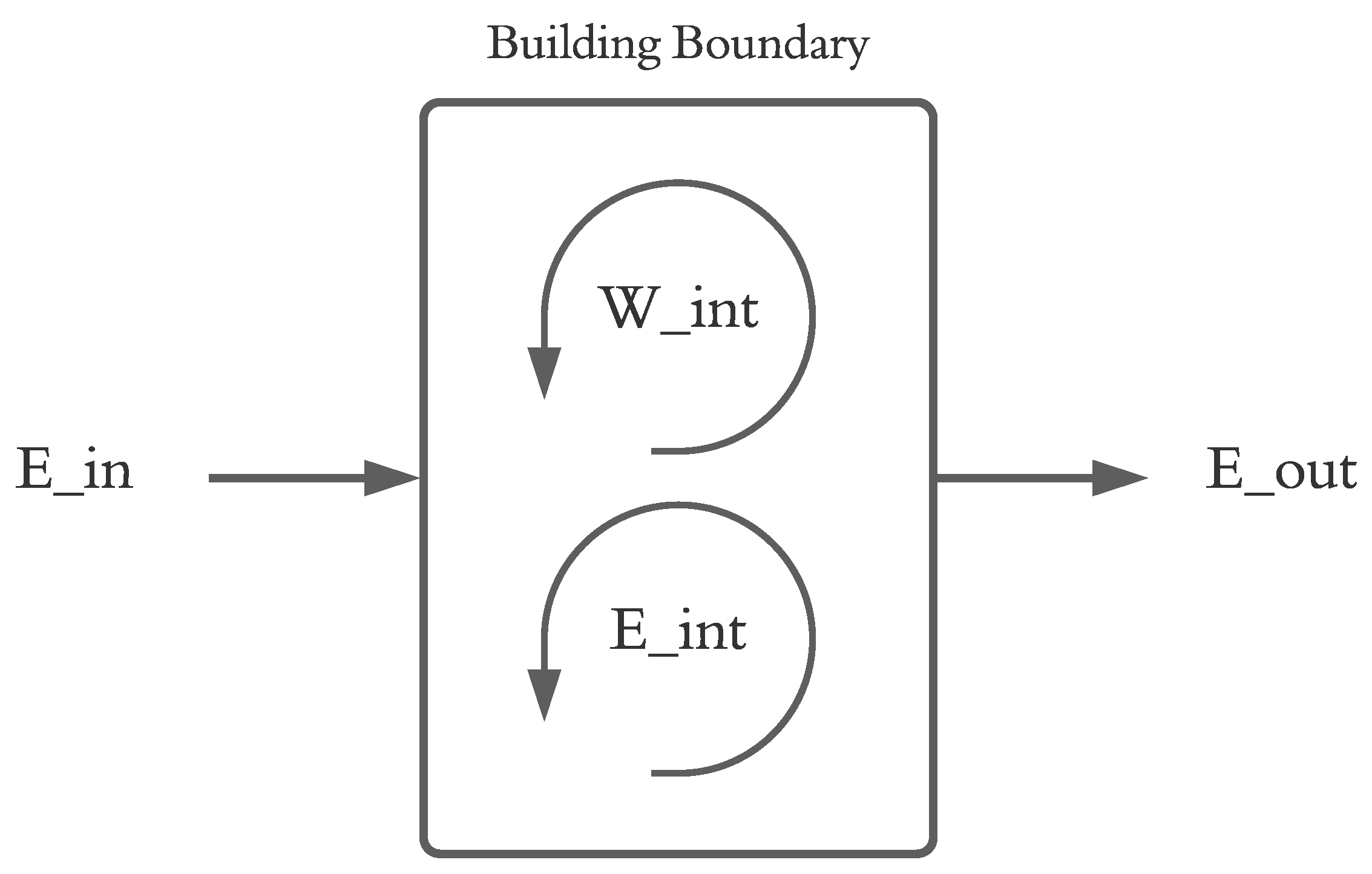
Figure 2.
Building energy harvesting resource flowchart.
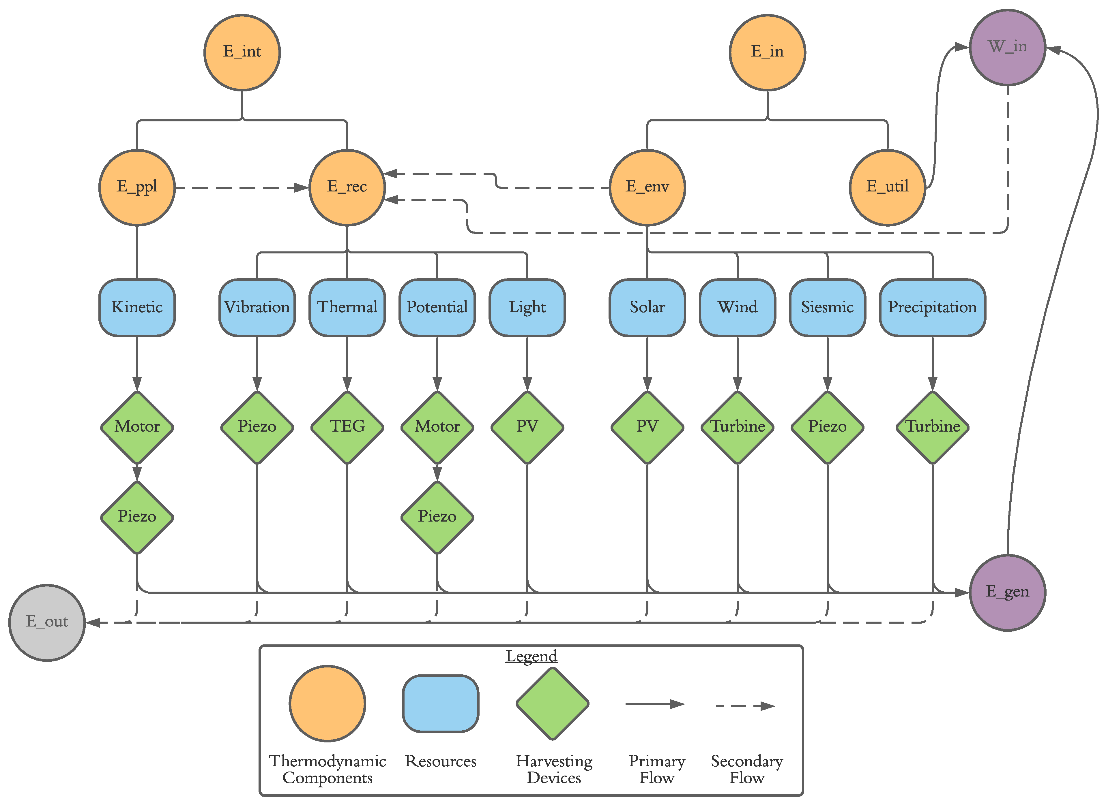
Figure 3.
Sun path diagram for Toronto, Ontario, Canada.
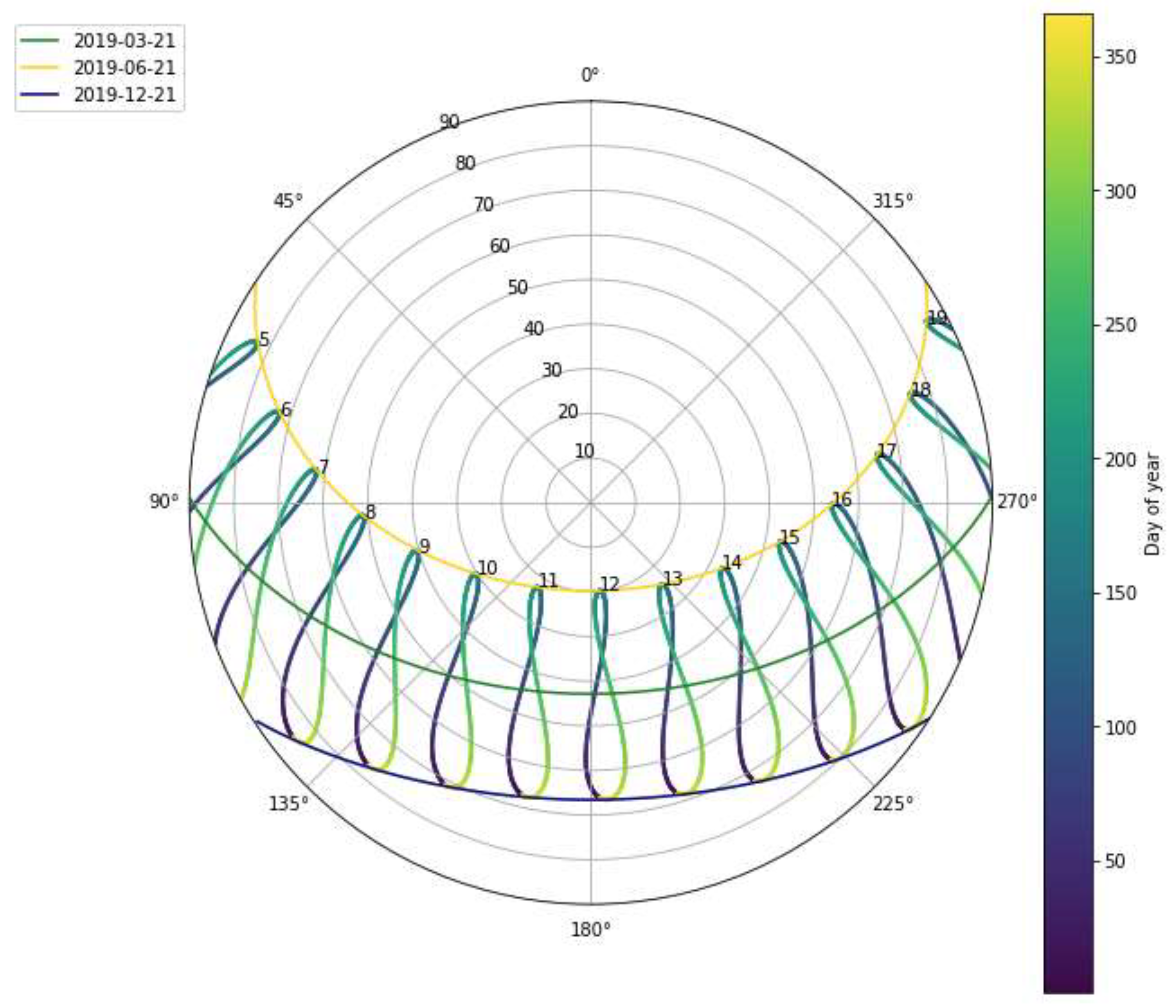
Figure 4.
Wind Rose for the case study location of Toronto, Ontario, Canada.
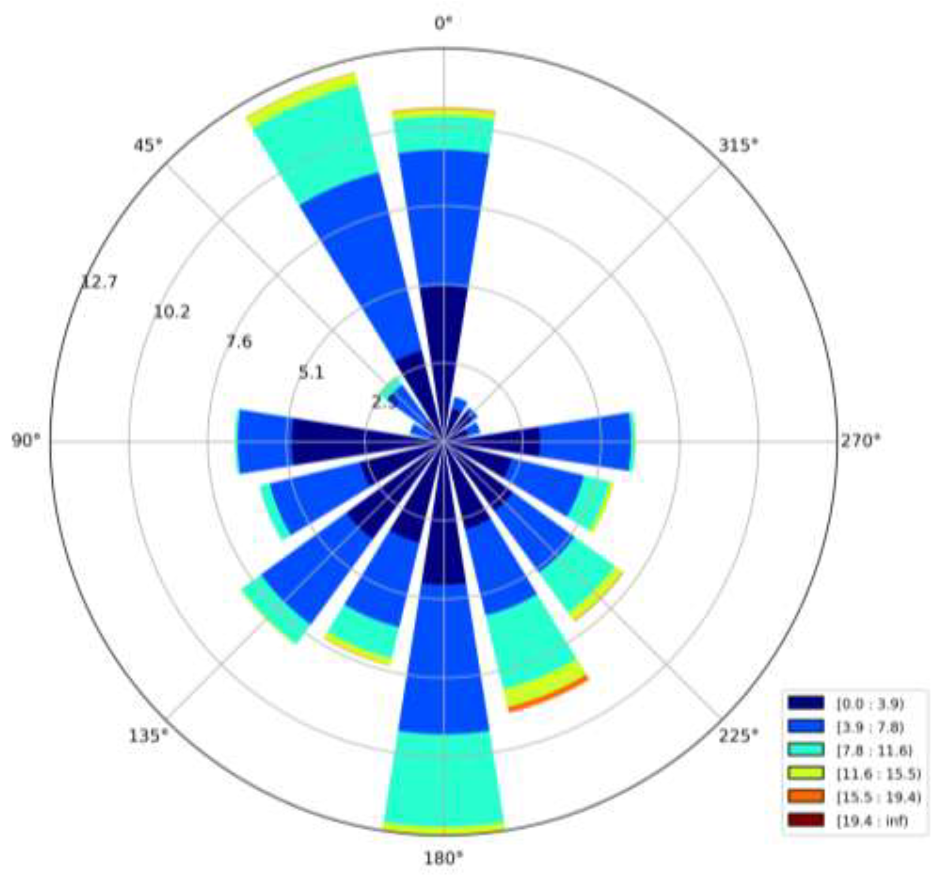
Figure 5.
Wind catchment area geometry.
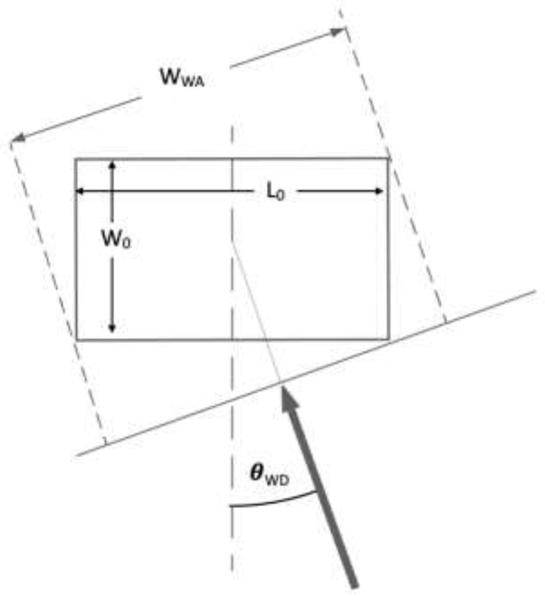
Figure 6.
Monthly variation in wind & solar resources at Billy Bishop weather station.
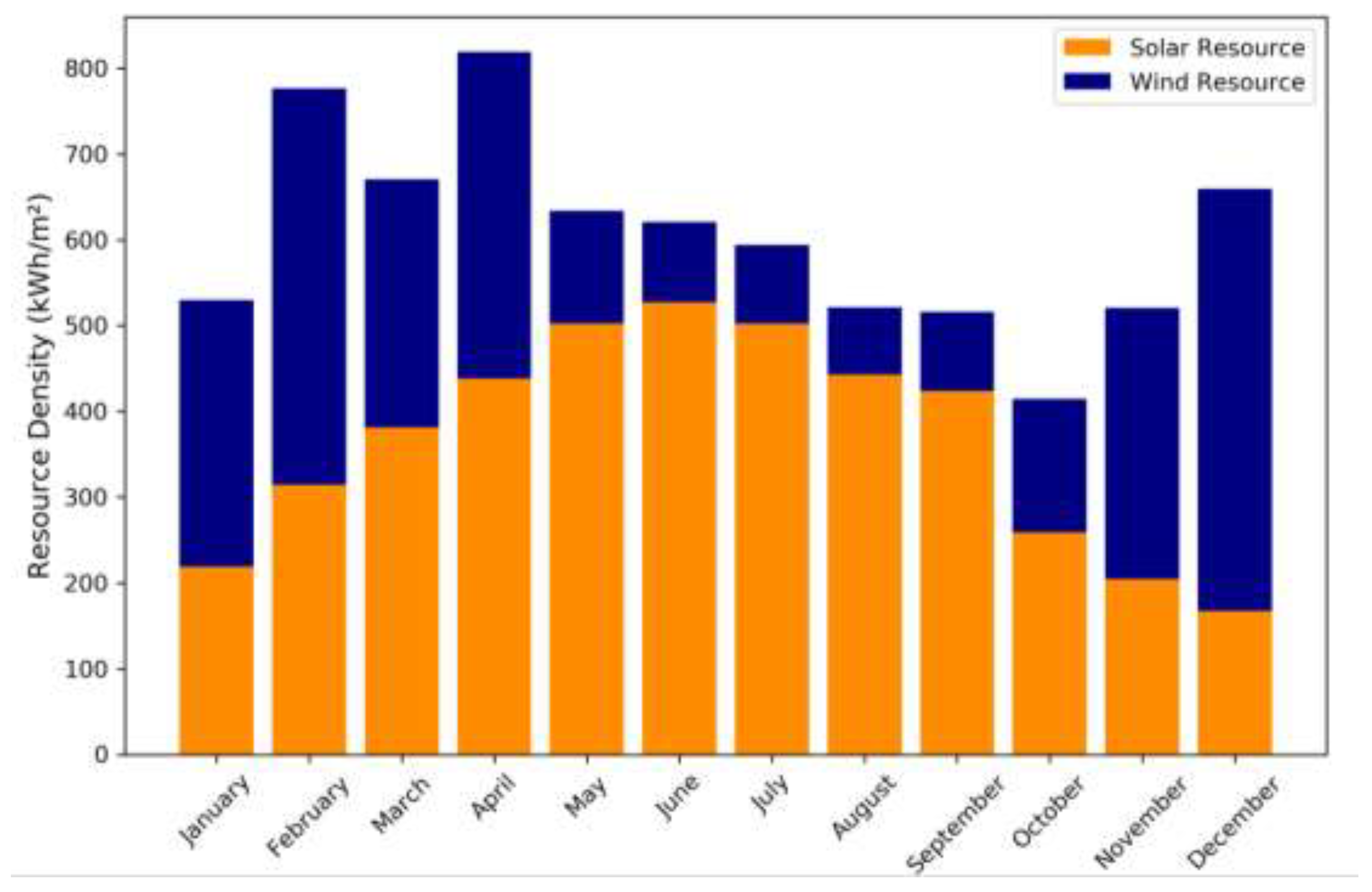
Figure 7.
External quantum efficiency of single crystalline Si and tandem junction photovoltaic cells [40].
Figure 7.
External quantum efficiency of single crystalline Si and tandem junction photovoltaic cells [40].
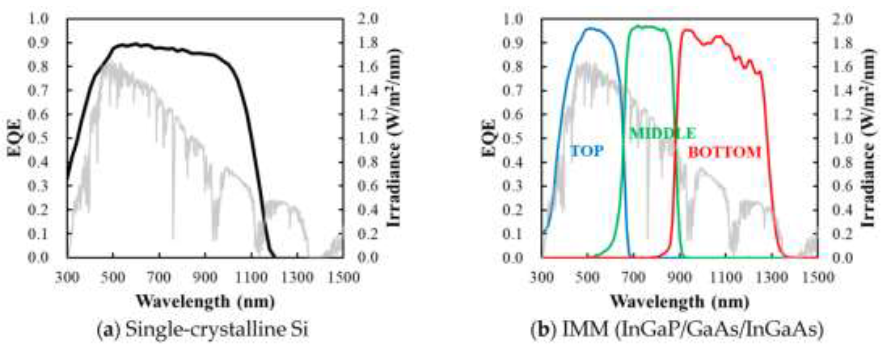
Figure 8.
Differentiation between Savonius and Darrieus VAWTs with twisted models included [52].
Figure 8.
Differentiation between Savonius and Darrieus VAWTs with twisted models included [52].
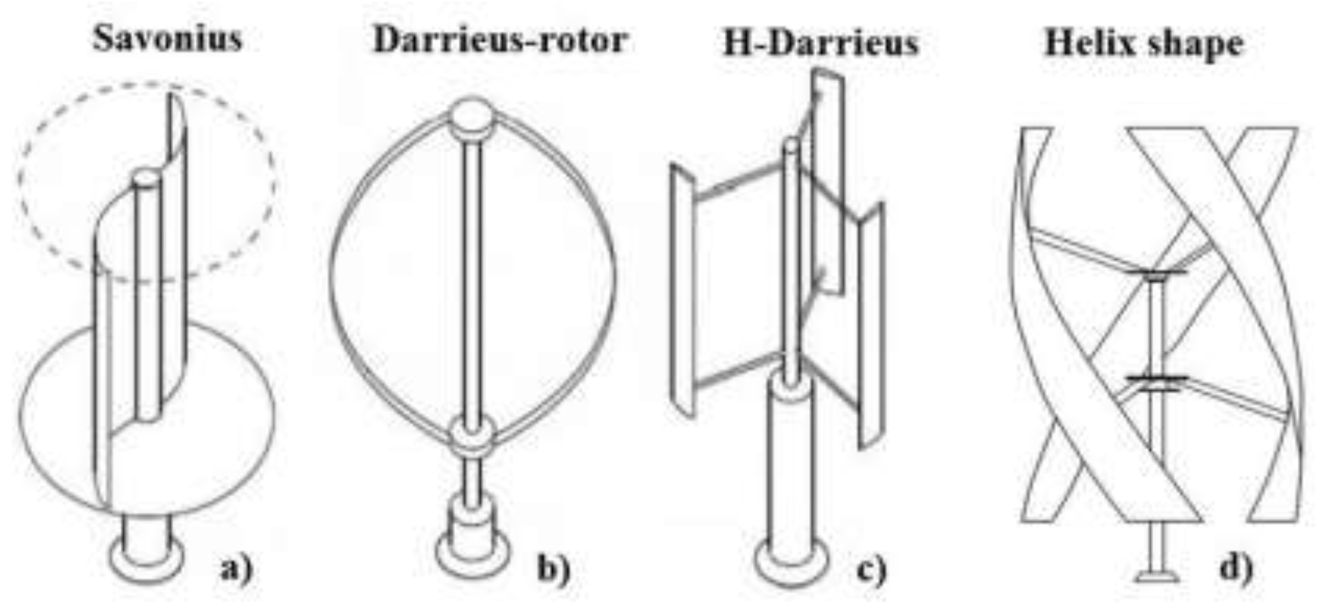
Figure 9.
Coupling modes of piezoelectric materials relating loading orientation to crystal geometry [18].
Figure 9.
Coupling modes of piezoelectric materials relating loading orientation to crystal geometry [18].
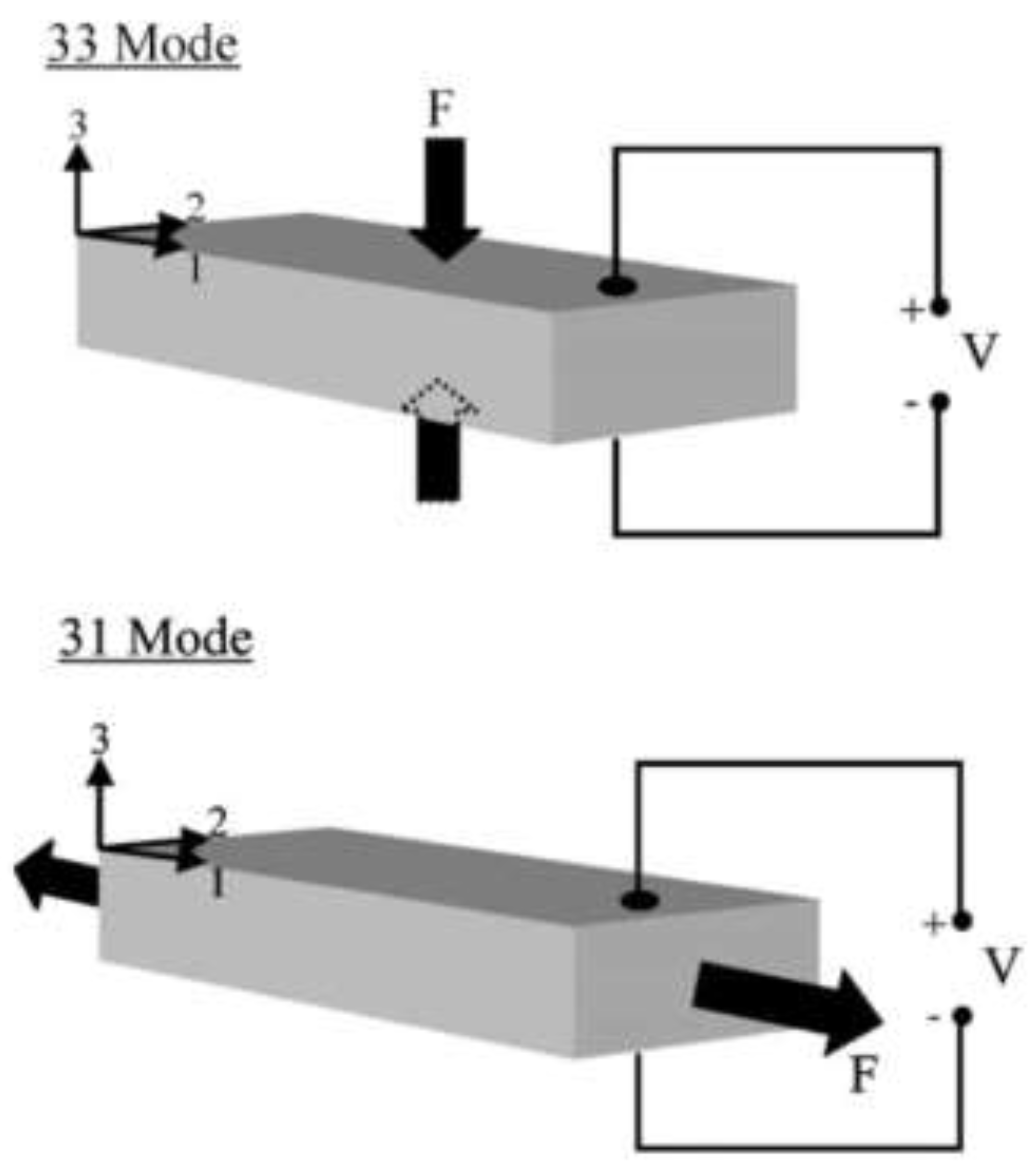
Figure 10.
Thermal resistance network governing 1D heat transfer through a thermoelectric generator.
Figure 10.
Thermal resistance network governing 1D heat transfer through a thermoelectric generator.
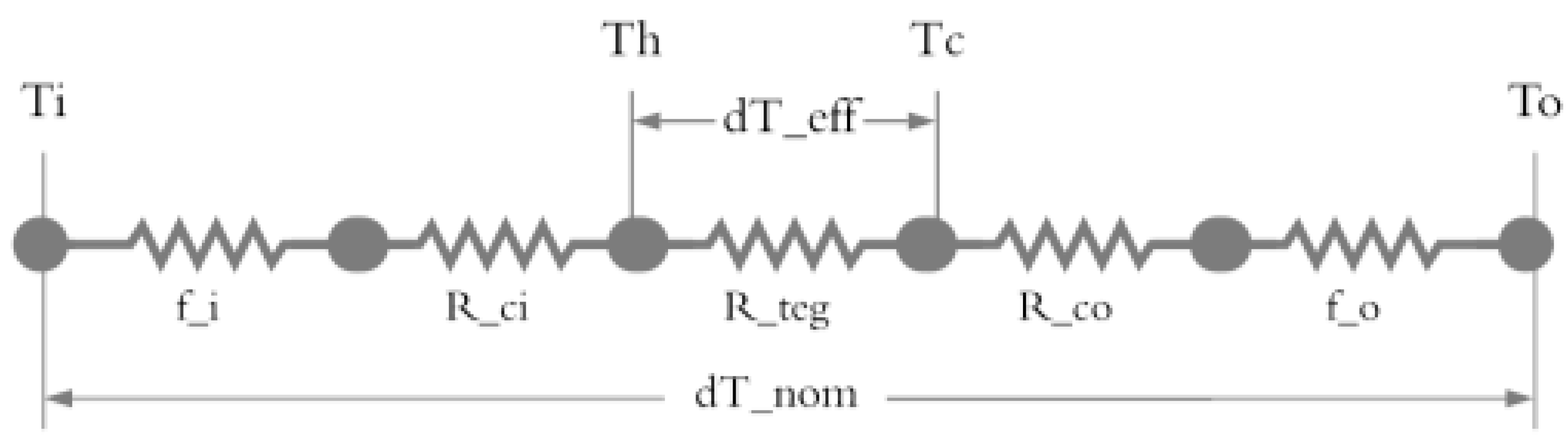
Figure 11.
Thermoelectric application reference indicating available power over a range of thermal gradients expected in buildings.
Figure 11.
Thermoelectric application reference indicating available power over a range of thermal gradients expected in buildings.
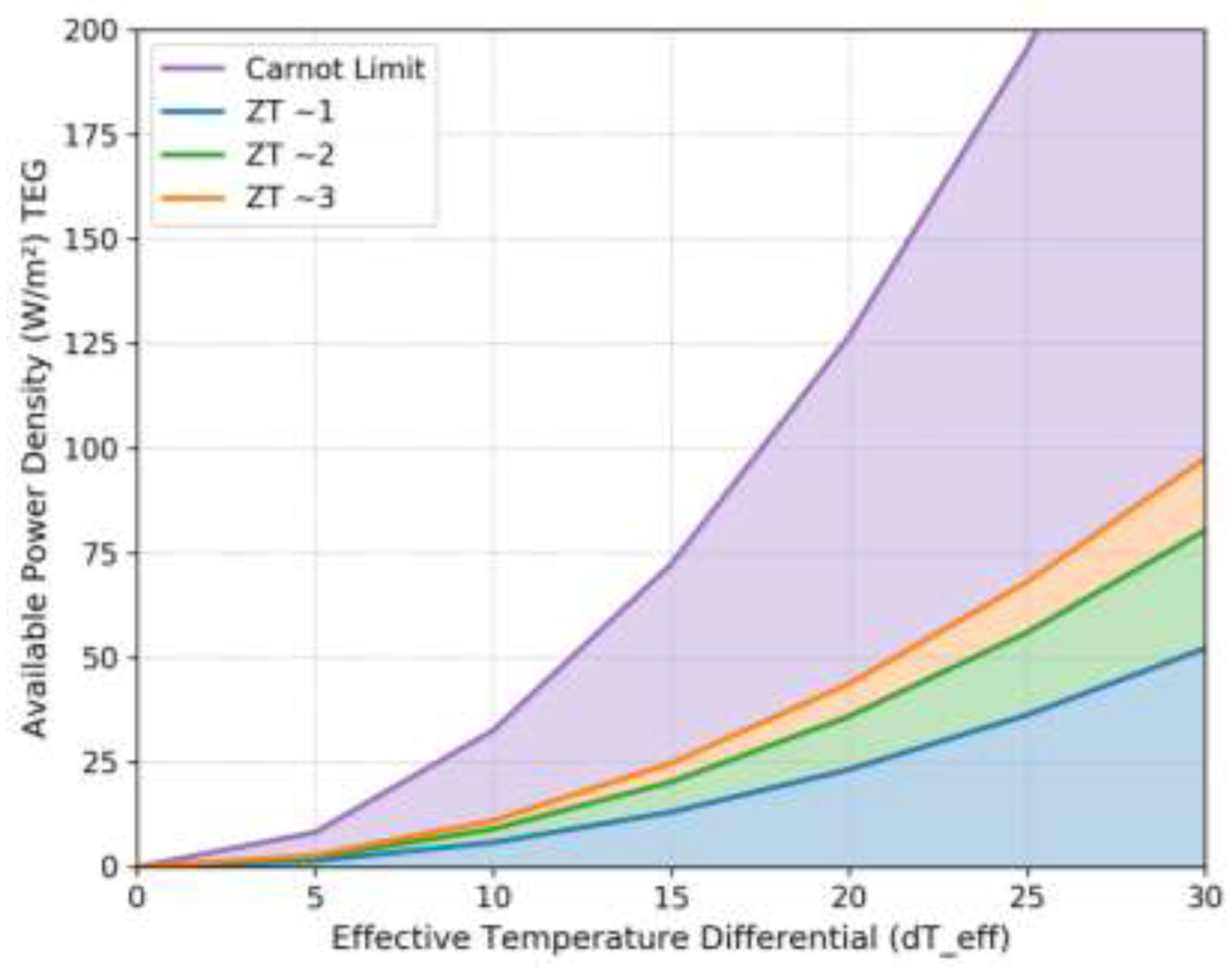
Figure 12.
Tiered classification of case study energy harvesting applications according to energy generation intensity.
Figure 12.
Tiered classification of case study energy harvesting applications according to energy generation intensity.
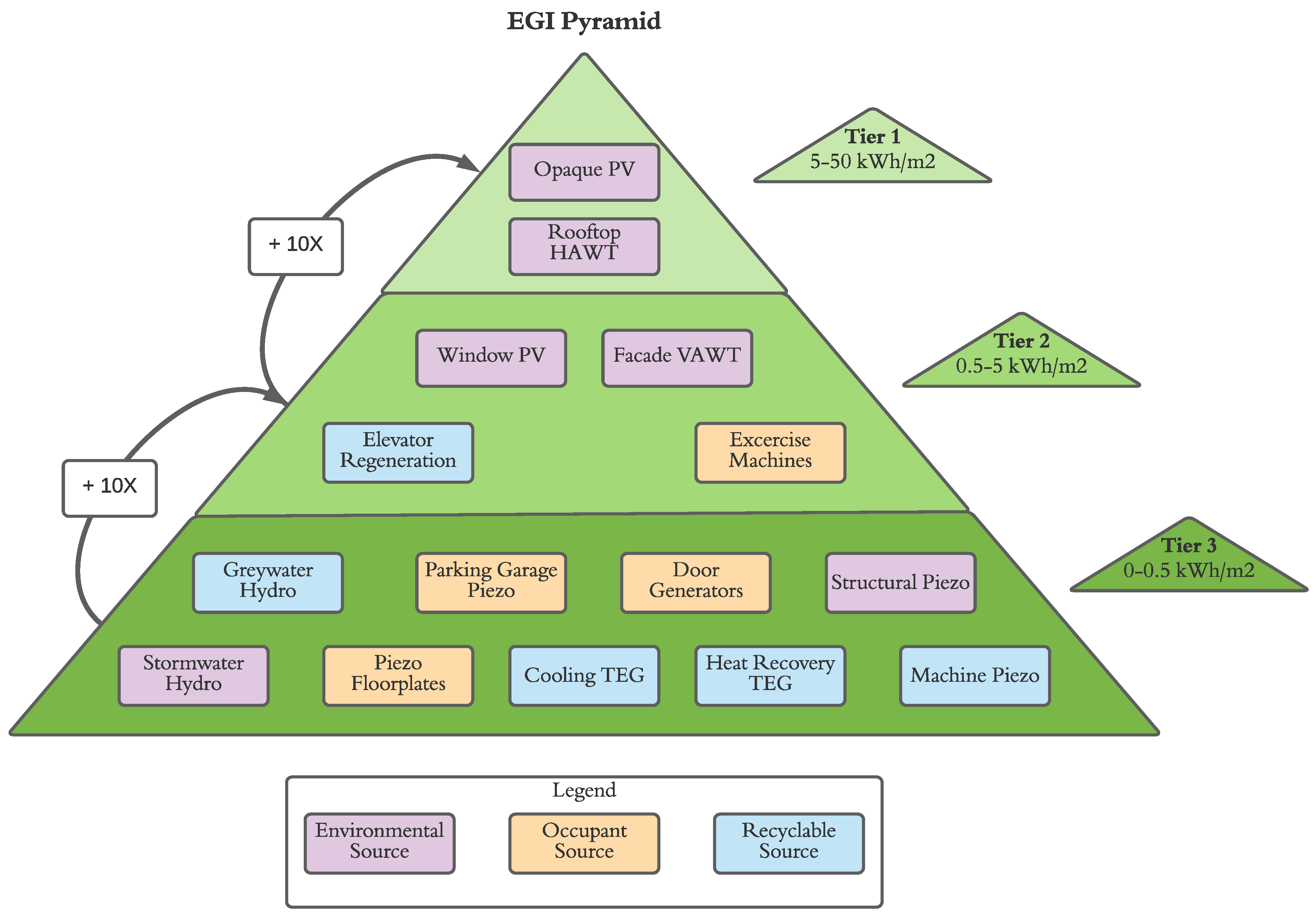
Figure 13.
Sankey diagram of energy resources and harvesting potential in case study building.
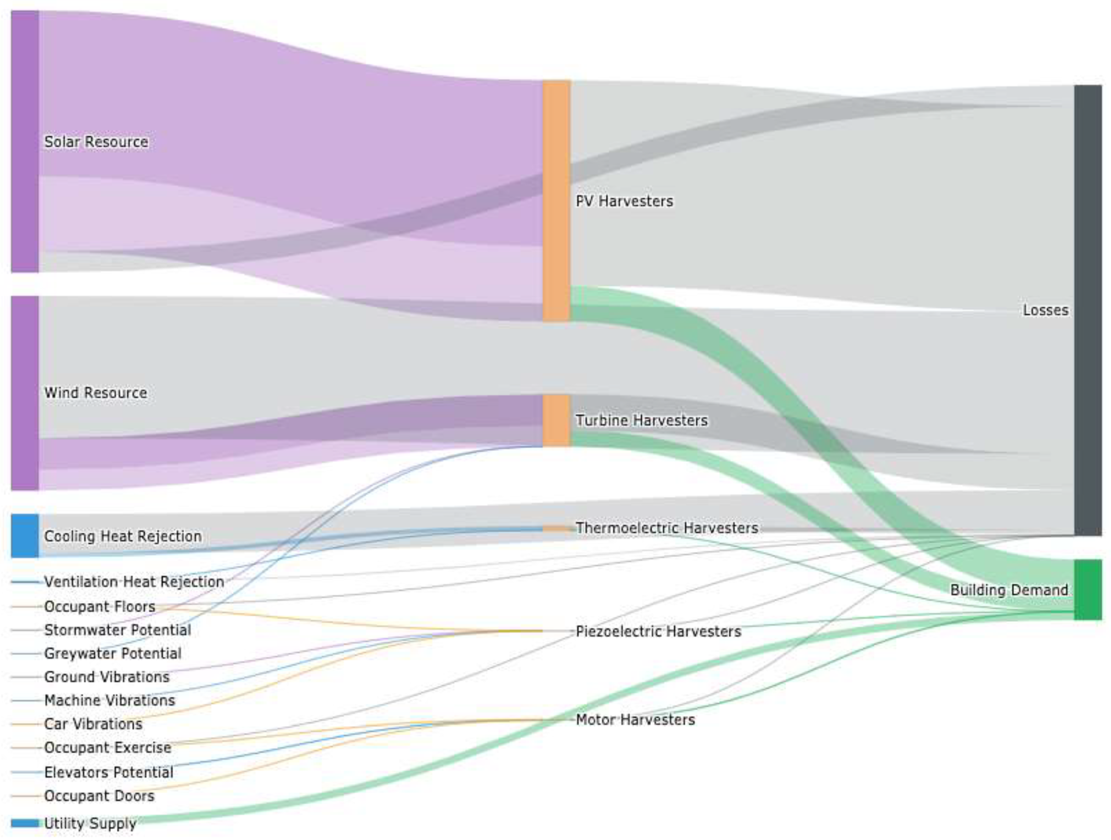
Figure 14.
Temporal alignment of various energy harvesting profiles with building load.
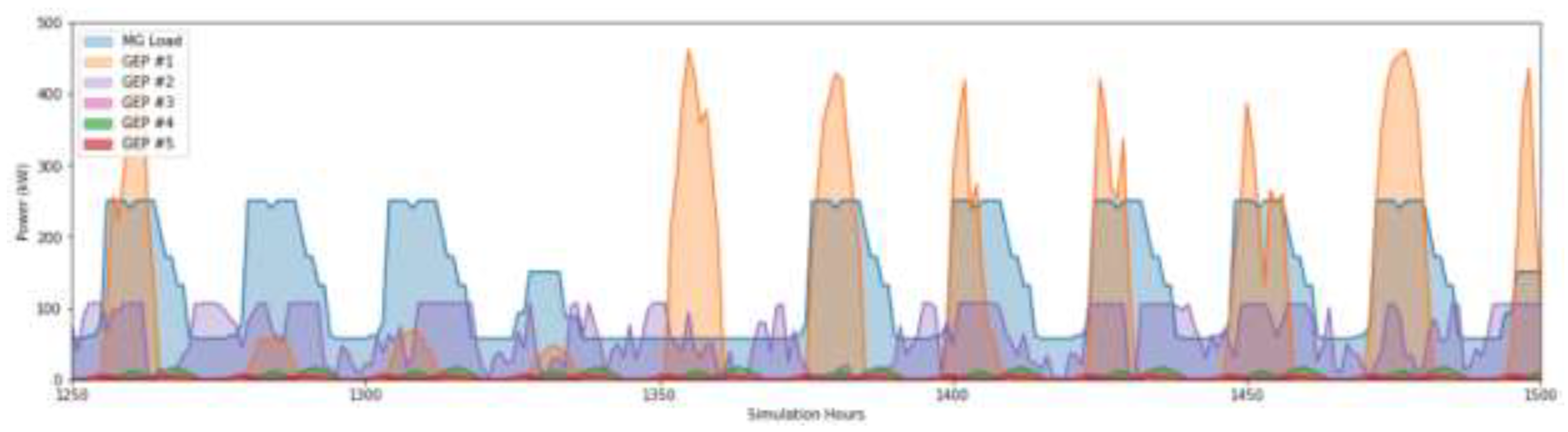
Table 1.
Total annual solar resource on cardinal building surfaces in Toronto.
| Orientation | Annual Solar Resource (kWh/m2) |
| South (90°) | 1189 |
| East (90°) | 927 |
| West (90°) | 880 |
| North (90°) | 451 |
| Horizontal (0°) | 1384 |
| Optimal Tilt (South 35°) | 1652 |
Table 2.
Average human power output for various exercise equipment [34].
Table 2.
Average human power output for various exercise equipment [34].
| Exercise Machine | Average Human Power (W) |
| Self-powered Treadmill | 100 |
| Elliptical | 100-150 |
| Stationary Bike | 50-150 |
| Rowing Machine | 160-200 |
Table 3.
Performance characteristics of various wind turbine typologies.
| Turbine Type | Average Cp | Reference | Yaw Control |
| HAWT | 0.35-0.4 | [47], [49] | Y |
| VAWT - Darrieus | 0.2-0.3 | [48], [49] | N |
| VAWT - Savonius | 0.1-0.2 | [48], [49] | N |
Table 4.
Case Study Building Properties.
| Floor Plate (m2) | 1858 |
| EUI (kWh/m2) | 97 |
| Length / Width (m) | 60.9 / 30.5 |
| Stories | 12 + 2 parking |
| Total Height (m) | 43.9 |
| Conditioned Floor Area (m2) | 22,304 |
| Occupancy (m2/pp) | 16 |
| Window-Wall Ratio | 50% |
| Opaque R-value (Rsi) | 3.93 (R22) |
| Window U-Value (W/m2K) | 2.96 |
| Window SHGC | 0.5 |
| Orientation | Due South |
Table 5.
Toronto’s Climate Data.
| Latitude (°) | 43.65 N |
| Climate Zone | 5A |
| Average Temperature (°C) | 9 |
| Max. Temperature (°C) | 32 |
| Min. Temperature (°C) | -20 |
| HDD (°C-days) | 3000-4000 |
| CDD (°C-days) | 200-600 |
Table 6.
Annual Energy Resource Assessment for Case Study Building in Toronto, ON.
| Resource | Subcategory | Annual Magnitude | Units | Ref. | Dependency |
| Solar | South | 1189 | kWh/m2 | [6] | Weather |
| East | 927 | kWh/m2 | [6] | Weather | |
| West | 880 | kWh/m2 | [6] | Weather | |
| North | 451 | kWh/m2 | [6] | Weather | |
| Roof | 1384 | kWh/m2 | [6] | Weather | |
| Wind | Total | 2893 | kWh/m2 | Weather | |
| Potential | Precipitation | 0.0022 | kWh/m2RAm | Weather | |
| Greywater | 0.0008 | kWh/m2FA m | [25], [27] | Demand | |
| Elevators | 0.2 | kWh/kWh | [28] | Demand | |
| Vibration | Ground | 295.5 | kWh/floor | [16] | Site |
| Machinery | 0.01 | kWh/kWhHVAC | [18] | Demand | |
| Vehicles | 0.048 | kWh/car | [68] | Occupants | |
| Occupants | Exercise | 15.6 | kWh/pp | [32] | Occupants |
| Doors | 0.002 | kWh/door/pp | [33], [34] | Occupants | |
| Floors | 0.29 | kWh/pp | [35], [36] | Occupants | |
| Thermal | Cooling | 4 | kWh/kWhCool | Demand | |
| Ventilation | 0.333 | kWh/kWhHR | Demand | ||
| Lighting | Total | 2 | kWh/m2FA | [9] | Demand |
Disclaimer/Publisher’s Note: The statements, opinions and data contained in all publications are solely those of the individual author(s) and contributor(s) and not of MDPI and/or the editor(s). MDPI and/or the editor(s) disclaim responsibility for any injury to people or property resulting from any ideas, methods, instructions or products referred to in the content. |
© 2025 by the authors. Licensee MDPI, Basel, Switzerland. This article is an open access article distributed under the terms and conditions of the Creative Commons Attribution (CC BY) license (http://creativecommons.org/licenses/by/4.0/).
Copyright: This open access article is published under a Creative Commons CC BY 4.0 license, which permit the free download, distribution, and reuse, provided that the author and preprint are cited in any reuse.


