
Submitted:
10 March 2025
Posted:
11 March 2025
You are already at the latest version
Abstract
As SLAM technology has evolved from the geometric level to the object level, Active SLAM (ASLAM) has also adopted a new goal: improving the ability to observe objects. However, current ASLAM mostly focuses on low-dimensional environmental features such as points, lines, and planes, while ignores the impact of motion process on SLAM. This paper proposes a new observation pose optimization method based on the ellipsoid model and the camera field of view to enhance the robot’s ability to observe objects. We integrate view planning and motion planning into a unified observation pose optimization module and construct an optimized factor graph based on probabilistic inference. Our method ensures the observation poses are globally optimal and can directly generate robot control variables. Leveraging the camera’s field of view and the ellipsoid model abstracted from object SDF model, we introduce three key factors into the factor graph: object completeness observation factor, self-observation prevention factor, camera motion smoothness factor. Finally, we develop the object ASLAM system with our observation pose optimization method, and evaluate it in multiple simulation environments. Experimental results demonstrate that our method significantly improves object modeling accuracy, mapping efficiency, and localization precision. The code for this work are open-sourced at https://github.com/TINY-KE/OPO_ASLAM.git.
Keywords:
observation pose optimization
; active SLAM
; object SLAM
; view planning
1. Introduction
Active SLAM (ASLAM) is a technique designed to improve SLAM accuracy and efficiency. By combining perception and motion planning, ASLAM can select autonomously the optimal observation trajectory to maximize information gain. Its core objectives include:(1) Intelligently selecting the optimal observation positions to acquire the most informative perception. (2) Optimizing observation trajectories to reduce localization uncertainty, enhance the robustness and mapping accuracy of the SLAM system.
However, Active SLAM has not kept pace with the recent advancements in SLAM technology. While SLAM has evolved from a geometric paradigm to an object-level paradigm, Active SLAM remains primarily focused on lower-dimensional geometric features such as points, lines, and planes.
Object features serve as robust landmarks that incorporate semantic, shape, pose, and texture information, while maintaining spatial geometric constraints. Object SLAM aggregates low-level geometric primitives (e.g., voxels, point clouds) into a single object instance, ultimately constructing an object-level map. By integrating accurate object models into SLAM’s back-end, the robustness and accuracy of SLAM are significantly improved. Additionally, Object SLAM enhances the robot’s semantic understanding of its environment. Common modeling techniques in Object SLAM include DeepSDF[1], MaskFusion[2], etc.
Since the quality of object modeling is influenced by the observation view, Active SLAM has taken on a new mission—improving the ability to observe objects. Object modeling require multi-angle continuous observations to ensure complete information acquisition, because objects are three-dimensional entities. Otherwise, the issue of unobservability[3] will occur, leading to inaccurate size and depth estimation of object models. The ideal observation trajectory should involve continuous observations around the object. Object modeling relies on low-level geometric features and requires frame-to-frame alignment, data association, and object detection. Achieving complete observation within a single frame can help mitigate accumulated errors, reduce data association errors, and enhance object recognition accuracy. To support the Object SLAM, it is essential to ensure multi-angle observations and single-frame complete observation when observes objects.
Traditional Active SLAM primarily processes low-dimensional environmental features such as points, lines, and planes, and ignores the objects. The view planning strategies, as the key component of the conventional ASLAM, can be categorized into frontier-based exploration methods [4] and information entropy-based methods [5]. The entropy-based approach treats environmental uncertainty as an optimization objective by prioritizing views that minimize entropy, selecting the Next Best View (NBV). Entropy calculations can be performed using Bayesian updating [6], which infers map uncertainty, or mutual information maximization [7], which assesses the correlation between current observations and prior maps using occupancy grid maps or octree maps. However, both methods overlook object-level features. Although some methods, such as Active-EAO-SLAM [8] and VP-SOM [9], have considered active object observation, they are mostly limited to small tabletop objects, making them unsuitable for more complex real-world environments.
Additionally, view planning and motion planning are decoupled in traditional ASLAM. Motion planning merely serves the NBV output from view planning, without considering the impact of motion process on the object observation. For example, the robot’s own body may occlude the camera’s FOV (field of view), or the camera may lose sight of the target object due to excessive movement.
To address these challenges, we propose a new observation pose optimization algorithm based on the ellipsoid model and camera FOV. For object models that require additional observations to be completed, we abstract them into ellipsoids, retaining only the pose and size information while discarding shape and texture. The ellipsoid model serves as prior information, facilitating the construction of constraints between the object and the camera’s FOV. Moreover, we integrate view planning and motion planning into a unified observation pose optimization module. The observation pose optimization module can directly output the robot’s control variables (e.g. chassis pose, robotic arm joint angles), ensuring that the observation views during the motion process are also constrained. We construct an optimized factor graph based on probabilistic inference for the observation pose optimization, ensuring the planned observation trajectory is globally optimal. Three key constraint factors are introduced: object completeness observation factor, self-observation prevention factor, and camera motion smoothness factor. The constraint factors not only ensure a complete single-frame observation of the object, but also prevent the camera’s field of view from being obstructed by the robot’s body or moving too fast, which could degrade observation quality.
In summary, our contributions are as follows:
- We construct an unified observation pose optimization method to ensure the observation quality during motion.
- We build a factor graph for pose optimization to guarantee the global optimality of the observation trajectory.
- We construct the object completeness observation factor, self-observation prevention factor, and camera motion smoothness factor, based on the ellipsoid model and camera FOV.
- We validate our method through simulation experiments, demonstrating improvements in object modeling accuracy, exploration efficiency, and camera localization precision.
The remainder of this paper is structured as follows. Section 2 discusses view planning methods in Active SLAM, including information entropy-based approaches and object-aware strategies. Section 3 introduces the factor graph-based framework for object observation pose optimization. Section 4, Section 5 and Section 6 detail the construction of the three key optimization factors: object completeness observation factor, self-observation prevention factor, and camera motion smoothness factor. Section 7 presents experimental results and comparative analyses.
2. Related Work
2.1. Information-Entroy Based ASLAM
Shannon’s information entropy [10] serves as a measure of uncertainty and is widely used to assess map uncertainty. View-planning strategies leveraging information entropy typically select the Next Best View (NBV) that minimizes uncertainty most efficiently. Consequently, information gain, defined as the reduction in information entropy, is a key metric in these evaluation functions.
Early research [11] formulated candidate views based on map frontiers and the robot’s reachable space. Building on these ideas, Bourgault et al. [5] incorporated both map entropy and robot pose entropy into the view-evaluation framework. Map entropy was derived from occupancy probabilities in a grid map, while robot pose entropy was estimated using the covariance matrix from particle filter-based SLAM.
For graph-based SLAM, Carrillo et al. [12] explored Renyi entropy to quantify pose uncertainty. Later, Isler et al. [13] extended entropy-based techniques to 3D space, utilizing OctoMap voxel occupancy probabilities to compute entropy while factoring in camera FoV and object occlusion through weighted voxel assignments. Wang et al. [14] applied this 3D approach to large-scale industrial environments, while Zheng et al. [15] introduced semantic segmentation entropy, considering semantic labels of voxels and confidence probabilities.
Beyond entropy-based methods, the Theory of Optimal Experimental Design (TOED) also evaluates the utility of active mapping actions. In this approach, each action is modeled as a stochastic design, and comparisons are made using covariance matrices and optimality criteria such as A-opt, D-opt, and E-opt. Prior studies [16,17] examined the relationship between these optimality criteria and connectivity indices in active Graph-SLAM.
Although some studies, such as [15], have incorporated the semantic attributes of objects, they still do not treat objects as complete, unified entities. As a result, these approaches may lead to incomplete object observations, which can negatively impact the accuracy and consistency of object reconstruction.
2.2. Object Based ASLAM
Object-based ASLAM are generally categorized into model-based and model-free approaches, with the latter further divided into volumetric-based and surface-based methods [18], depending on object representation. Model-based methods [19,20] utilize prior knowledge of an object’s geometry or appearance, while model-free methods offer greater adaptability for object mapping. Surface-based approaches are effective for objects represented by curves or surfaces, such as triangle meshes [21], ellipsoidal surface fitting [22], and cross-sectional B-spline fitting [23]. Assuming spatial continuity, these methods predict unseen object surfaces using boundary detection and surface trend analysis.
Volumetric models, including octrees, TSDF, and cube-based representations, are widely used in object mapping, making volume-based methods prevalent in view planning. Early works, such as Wong et al. [24], selected the NBV by maximizing the visibility of unknown voxels, while Dornhege et al. [25] used voxel occupancy boundaries for selection. More recent approaches prioritize volume information gain (VI). Isler et al. [13] reviewed five VI computation methods, including occlusion-aware VI, which considers voxel occlusion, unobserved voxel VI, which explores unknown areas, and rear-side entropy VI, which directs views behind objects. Monica et al. [26] adapted frontier exploration for TSDF models, while Wu et al. [27] proposed projecting internal points onto surfaces, using a surface grid map where grid entropy reflects object model completeness. Patten et al. [28] focus on individual objects or small clusters, lacking adaptability to complex indoor environments.
The above methods fail to achieve complete object observation because they cannot establish a comprehensive observation model that accounts for both complex object structures and the camera’s field of view. To address this, we abstract the object model using an ellipsoid representation. Moreover, these methods ensure optimal observation only at the NBV but fail to maintain it during motion. This limitation arises from the separation of view planning and motion planning. In contrast, we overcome this issue by integrating both into a unified observation pose optimization module.
3. Factor Graph for Object Observation Pose Optimization
3.1. Scenario Analysis for Active Object SLAM
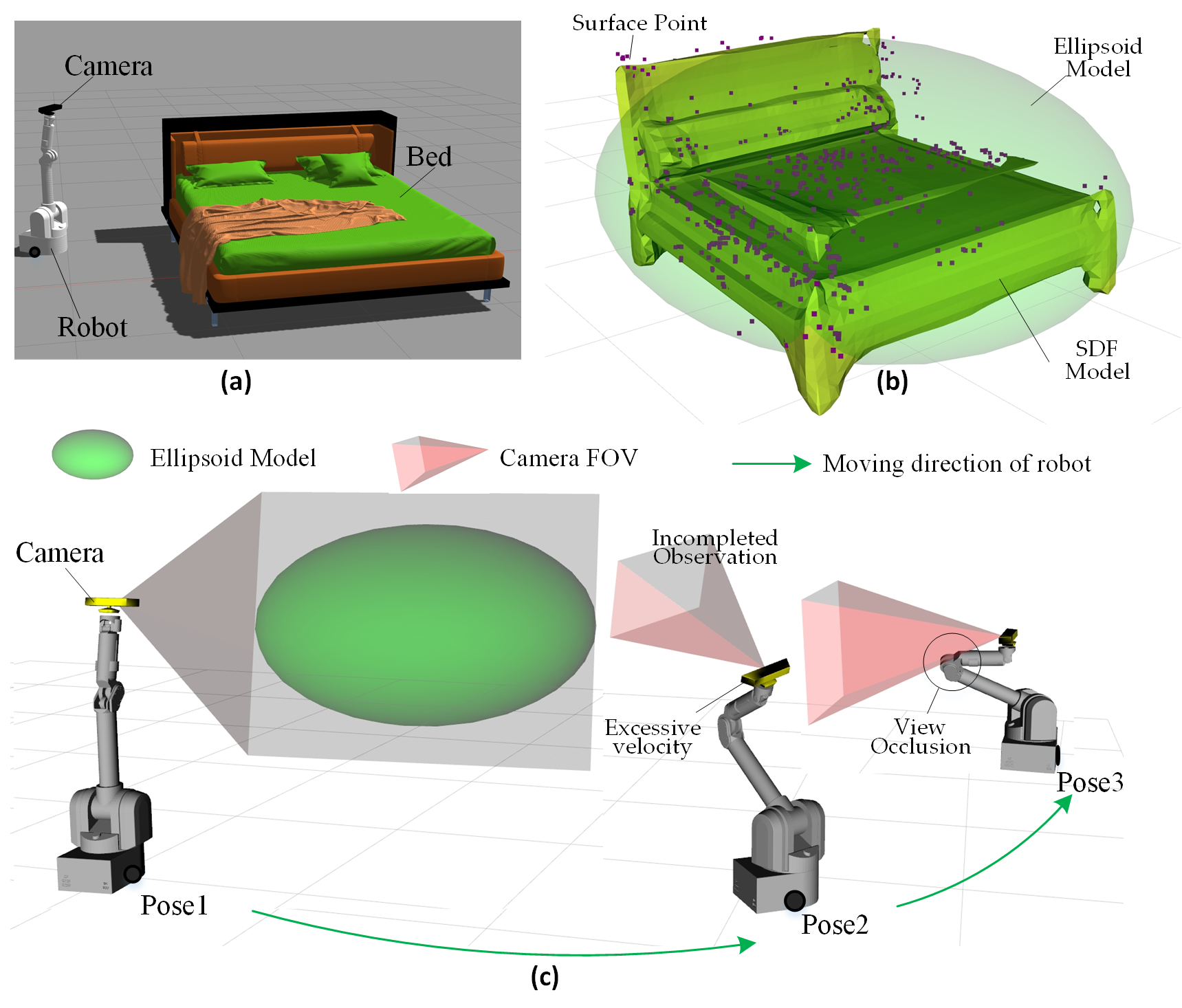
Figure 1 illustrates a typical scenario where a mobile robot constructs an object model using Active Object SLAM. The robot platform equipped with a camera and the target object (a bed) are shown in Figure 1a. The robot performs a series of observations around the bed and eventually constructs its object model, as depicted in Figure 1b. Figure 1c demonstrates the robot’s autonomous object observation process, highlighting three typical observation poses.
The observation platform consists of a robot platform and an end-mounted camera. The mobile platform can take various forms, such as a mobile robot, UAV, or robotic arm. In this study, we use a differential-drive platform with a robotic arm (as shown in Figure 1) to analyze the active object SLAM scenario. The robot moves within the environment using its chassis, while the robotic arm adjusts the camera’s pose relative to the chassis. This enables the camera to observe objects from any position.
The camera has a FOV, which in 3D space is represented as a pyramid-shaped frustum extending along the camera’s z-axis from the camera center (depicted as the red frustum in Figure 1). The robot performs circular observations around the bed (green trajectory in Figure 1c), capturing multi-angle views of the object to obtain more complete information and improve the quality of the object model.
The object model contains information such as: Shape details,Dimensions, Center coordinates, Orientation, Semantic labels. We employ DeepSDF [1] to construct the Signed Distance Function (SDF) model of the object (yellow model in Figure 1b). The key idea of DeepSDF is to use implicit shape encoding to fit the 3D surface points of the object (purple points in Figure 1b). Unlike traditional discrete representations, DeepSDF provides a continuous representation of 3D shapes and supports shape completion, allowing recovery of complete shapes from partial observations.
Although the SDF model inherently contains size, position, and orientation information, it does not align well with human intuitive understanding. Moreover, the complex shape of the SDF model makes it challenging to impose constraints based on the camera’s FOV.
To address this, we introduce an ellipsoid model (green ellipsoid in Figure 1b). The three axes of the ellipsoidrepresent the object’s dimensions, while the ellipsoid’s center coordinates and orientation match those of the SDF model. It is important to note that, unlike previous works that construct ellipsoids using multi-view geometry [31] techniques, our ellipsoid model is directly extracted from the SDF model.
From the autonomous observation process shown in Figure 1c, we can summarize four types of observation risks.
- Incomplete Observation: The bed is a large object, making it easy to extend beyond the camera’s FOV, leading to incomplete observations. This increases frame-to-frame tracking errors, reduces object association accuracy. The incomplete observation may result in incorrect object modeling or split the model into multiple erroneous parts. This is a critical issue that must be avoided in object modeling. In Figure 1c, the camera at Pose1 has a complete view of the bed, ensuring full observation. However, at Pose2, the camera is in an upward-tilted pose, capturing only part of the bed, leading to incomplete observation.
- Robot Self-Occlusion of the Camera: In real-world scenarios, robots often have complex shapes and structures, which can lead to self-occlusion of the camera. In Figure 1, the robot includes a 7-DoF robotic arm, and during movement, it is difficult to prevent parts of the robot body from entering the camera’s FOV (as shown by the Pose3 in Figure 1c). This reduces the effective observation range and increases the risk of incorrect feature extraction, object detection and SLAM crush.
- Poor Camera motion smoothness: In Figure 1c, the three observation poses have large differences in the robot’s chassis position and arm joint angles. This results in abrupt changes in the camera’s motion trajectory and excessively high speeds during camera movement. Unstable camera motion may lead to failures in the feature extraction and inter-frame tracking of SLAM. Therefore, maintaining smoothness in both camera position and velocity is crucial for SLAM.
- Disconnection Between View planning and Motion Planning: In traditional Active SLAM, motion planning only serves the results of view planning, while neglecting the impact of the motion process on observation quality. As a result, during transitions between different observation poses, many issues such as incomplete object observation, self-occlusion of the camera, and motion oscillations may unpredictably occur.
To address the above issues, this paper proposes a new observation pose optimization method to reduce these risks.
3.2. Observation Pose Optimization Based on Probabilistic Inference
Observation pose optimization, as an advanced form of trajectory optimization, can be modeled as a Bayesian probabilistic inference problem: treating the continuous-time trajectory as a Gaussian process random variable and optimizing the trajectory through Maximum A Posteriori Estimation (MAP) under the constraints of prior poses (Prior) and observation data (Likelihood) to meet specific task requirements.
Trajectory Modeling: The trajectory is modeled as a vector-valued Gaussian Process (GP), with its prior distribution given by . where: is the vector-valued mean function, representing the expected value of the trajectory. is the matrix-valued covariance function, describing the correlation between different time points. At discrete time points , the trajectory state Θ follows a joint Gaussian distribution.
The likelihood function: is used to encode task constraints, such as trajectory tracking [30] and obstacle avoidance. The likelihood function is generally modeled as an exponential family distribution:
where, is the residual function, measuring the deviation of the state from the task objective . The covariance matrix describes the scale and uncertainty of the error, which is typically related to measurement noise.
Computing the MAP Trajectory: Based on the given equations (1)-(2), compute the Maximum A Posteriori (MAP) trajectory :
Thus, the MAP estimation problem can be simplified into a nonlinear least squares problem, which can be solved using methods such as Gauss-Newton or Levenberg-Marquardt.
Factor Graph: Using a factor graph [29], the MAP trajectory estimation can be performed more efficiently. The prior function and likelihood function can be factorized into a product of functions and organized into a bipartite factor graph .
where, the prior nodes represent a set of discrete trajectory poses over continuous time. The factor nodes are a set of functions acting on subsets of variables Θᵢ ⊆ Θ, and represents the edges connecting these two types of nodes. Thus, we can express the posterior distribution as a product of factors that jointly represent both the prior and the likelihood :
We construct the observation pose optimization module as a factor graph, as shown in Figure 2, which includes prior pose nodes and several factor nodes: the object completeness Observation factor , the self-observation prevention factor , the camera motion smoothness factor , the start pose constraint factor and the end pose constraint factor .
The gray nodes represent the mobile robot states , where . We adopt the constant velocity model. The chassis state is defined as , where represents the chassis pose, and represents the chassis velocity. The joint state is defined as , where represents the joint angle, and represents the joint angular velocity. The yellow circle at the center of Figure 2 represents the target object .
The blue triangles represent the object completeness observation factors, which exist between the robot states and the currently observed target object . Object completeness observation factors help prevent incomplete object observations. It is important to note that the object completeness observation factors only affect the robot state and do not directly modify the object model parameters. The green squares represent the self-observation prevention factors, which exist within a single robot state and help prevent the robot body from obstructing the camera’s FOV. The red circles represent the camera motion smoothness factors, which exist between two consecutive robot states. The camera motion smoothness factors ensure smooth camera motion by controlling the robot’s movement during the observation phase, preventing oscillations and sudden accelerations. These factors will be discussed in detail in Section 4, Section 5 and Section 6.
Using the factor graph illustrated in Figure 2, we integrate view planning and trajectory planning into a unified framework. This allows the robot to simultaneously optimize both the observation views and motion trajectory during autonomous observation. Compared to traditional methods, our approach globally constrains the robot state within the factor graph and ensures the complete object observation in one frame, the prevention of self-occlusion, and the smooth camera motion. As a result, our method achieves global optimality in the active SLAM process, improving mapping accuracy and exploration efficiency.
4. Object Completeness Observation Factor
4.1. Construction Idea
After the initial establishment of object SDF model by DeepSDF [1], there are still many details that need to be refined, such as missing regions in the model. To complete the missing information, the active SLAM system needs to move around the object and achieve complete observation in a single frame.
To ensure complete object observation, two key requirements must be satisfied:
- The object must be within the camera’s FOV.
- The object must not be too far from the camera.
In Figure 3b, when the camera is too close to the object or not facing it properly, the object in the image appears incomplete. In this case, the error in object segmentation increases, and the 3D feature points on the object’s surface are also partially missing, leading to an incorrect object model. Additionally, too-close observation needs further inter-frame associate and fuse of object feature points, which further increases the error. In Figure 3c, when the object is too far from the camera, the error in extracting 3D feature points and object segmentation increases significantly. Moreover, the number of extracted feature points is also noticeably reduced.
Based on the above analysis, we define complete object observation as the condition where the object model is tangent to the four planes of the camera’s FOV, as illustrated in Figure 4. In our work, the object model is represented in two forms: SDF model and ellipsoid model. To facilitate the computation of the spatial relationship between the field-of-view planes and the object, we use only the ellipsoid model to represent the object when constructing the object completeness observation factor.
To determine whether the object is tangent to the field-of-view (FOV) planes, there are two possible approaches: (1) direct computation in 3D space, which aligns with human intuition but has a high computational cost; (2) projecting the ellipsoid onto the camera plane, then comparing the projected ellipse (the green ellipse in Figure 5) with the FOV boundary box (the red dashed lines in Figure 5). We adopt the second approach, which has lower computational complexity.
Figure 5 illustrates the projection of the FOV-plane and object. The camera is represented by the combination of the camera center and the Image plane. The green ellipsoid represents the object model. The gray cone visualizes the projection process from 3D space to the 2D image plane. The green ellipse is the projection of ellipsoid. In our work, we do not directly use the maximum FOV angle of the original camera. Instead, we narrow the FOV to avoid distortion at the image edges. The four FOV planes correspond to four projected lines (the red dashed lines in Figure 5), which together form the FOV box.
According to multi-view geometry [31], the projection relationship between the plane in the camera coordinate system and the line in the image plane :
where represents the camera intrinsic matrix.
4.2. Relationship Between the Ellipsoid and the Plane
Ellipsoid Model: For a 3D point on the surace of an ellipsoid, the following equation holds:
where control the shape (scale) of the ellipsoid along the directions. influence the rotation of the ellipsoid. affect the position of the ellipsoid. , as a constant term, affects the overall scaling. Although this equation contains 10 parameters, multiplying both sides by a scalar does not change the equation. Therefore, the ellipsoid surface actually has 9 degrees of freedom. To express the ellipsoid equation more compactly, we introduce a symmetric matrix :
Equation (8) can then be rewritten as: , where is a symmetric matrix satisfying .
The ellipsoid’s pose relative to the camera coordinate system and the three axis lengths are obtained from object SLAM and object SDF models. The standard ellipsoid equation can be constructed by :
which can be rewritten in matrix form as , where is the representation of the ellipsoid model in the object coordinate system:
Ellipsoid Transformation: According to multi-view geometry [31], the ellipsoid model in the camera coordinate system is given by
The relationship of Ellipsoid and FOV Plane: when the camera’s FOV plane is tangent to the ellipsoid , the following equation holds:
where, .
Substituting equation (7) into the above, we obtain:
The four boundary lines of the FOV box satisfy:
where
and is the camera intrinsic matrix. Since the four edges of FOV box in the image plane are either horizontal or vertical, the line equations take the form or . Substituting these into equation (15), we obtain:
where represents the entry of G*. These four solutions correspond to the left, right, top, and bottom coordinates of the ellipsoid’s projected bounding box: , while the FOV box is: .
The deviation between the ellipsoid’s projected bounding box and the FOV box is: . The smaller the deviation, the better the object completeness observation, as shown in Figure 6.
4.3. Factor Construction
The Object Completeness Observation Factor is defined as:
where denotes the uncertainty in the camera observation.
5. Self-Observation Prevention Factor
5.1. Construction Concept
The robot’s own features are mistakenly recognized as environmental features, which can lead to the SLAM system crash. In traditional robotic platforms, cameras are typically mounted on the top or chest to avoid occlusion within the FOV. However, modern service robots are often equipped with robotic arms, introducing kinematic complexity that makes it difficult to completely avoid the robot’s body obstructing the camera’s view (as illustrated by the Pose3 in Figure 1c). To address this issue, we propose a method for constraining self-observation.
The core idea of this method is to treat each unit of the robot body as an avoidance unit (represented by yellow entities in Figure 7). When an avoidance unit approaches the camera’s FOV, a separation constraint is applied between the FOV plane and the avoidance unit, which drives the robot to adjust both its camera pose and its body pose, ensuring that the robot’s body moves out of the camera’s FOV.
As shown in Figure 7, the FOV is defined by four planes: top, bottom, left, and right. Clearly, it is sufficient for self-observation prevention, to ensure that the avoidance unit remains below the bottom plane of the FOV. Therefore, instead of handling all four planes simultaneously, we only compute the relative position between the robot body and the bottom FOV plane. This simplified strategy maintains system performance while significantly reducing computational cost, thereby improving the real-time capability and feasibility of the system.
We define the bottom plane as . is the normal vector of the plane. is the plane constant, determining the plane’s position in space. We define the normal vector points inward the FOV (as indicated by the blue arrow in Figure 8). For any point on the bottom plane, it must satisfy: .
5.2. Avoidance Sphere Coordinate Calculation Based on Robot Kinematics
To compute the interference relationship between the robot body and the camera’s field of view (FOV), it is necessary to perform appropriate geometric modeling of the robot body. In the field of robot obstacle avoidance, a commonly used approach is SDF-based modeling. This method allows for detailed modeling of complex robot geometries and supports precise obstacle avoidance calculations. However, in the construction of our self-observation prevention method, the robot’s geometric structure is relatively simple and regular. Therefore, we adopt a simple but effective modeling approach by attaching avoidance spheres to the robot body (as shown by the yellow spheres in Figure 8, with N = 8).
The avoidance sphere is defined as: , where denotes the radius of the avoidance sphere, indicates the link coordinate frame to which the avoidance sphere belongs, represents the pre-calibrated center coordinate of the avoidance sphere in link coordinate frame.
Advantages of the Avoidance sphere Model are as follows:
- Simplified Computation: By decomposing the robot body into a series of spheres, we can reduce computational complexity significantly.
- Efficient Mathematical Representation: Spheres and planes have simple mathematical forms. It’s easy for distance and gradient calculations.
The center of the avoidance sphere is given by:
where represents the homogeneous transformation matrix from coordinate frame to coordinate frame . We use the Denavit-Hartenberg (DH) method [32] for robot kinematics modeling in this paper.
5.3. Collision Detection
The shortest distance from the surface of the avoidance sphere to the bottom FOV plane is given by:
where is the radius of the avoidance sphere, representing the distance from the sphere’s center to its surface. is a manually set minimum safety distance between the plane and the sphere surface, which we define as 0.1 meter. represents the signed distance from the sphere center to the plane , calculated as:
where is the avoidance sphere center coordinate, expressed in homogeneous form. The notation represents the magnitude of a vector.
Note that both the bottom FOV plane and the avoidance sphere are defined in the robot coordinate system.
The distances of all avoidance spheres to the bottom FOV plane form the self-observation prevention error :
When , it indicates that the avoidance sphere is too close to the inner region of FOV.
5.4. Factor Construction
The Self-Observation Prevention Factor is defined as:
where represents the uncertainty of the factor. Since is influenced by both the robot’s motion and the camera’s field of view, considers both control errors and camera observation errors.
6. Camera Motion Smoothness Factor
The goal of Active SLAM includes improving environmental exploration efficiency and accelerating the mapping process. However, excessive movement speed can affect the smoothness of the camera motion, leading to degraded image quality, which in turn reduces the accuracy of the SLAM system.
Figure 9 illustrates the trade-off between efficiency and camera motion smoothness. The black-arrow trajectory exhibits large step movements and drastic velocity changes. The maximum speed in the Figure 9(c) exceeds the acceptable range for the SLAM system and negatively impacts the image quality captured by the end-mounted camera. Additionally, complete object observation fails in the Figure 9(b)(c). This type of issue has been highlighted in multiple studies about robot motion planning, such as [33]. In contrast, the red-arrow trajectory effectively mitigates excessive speed and incomplete object observation by inserting one intermediate pose (as shown in Figure 9f), thereby reducing the movement per step. However, adding more interpolation poses and limiting the maximum velocity significantly increases motion planning time and execution time.
To improve the smoothness of camera motion while maintaining exploration efficiency, we propose the following optimization strategies:
- Maintaining Temporal Consistency of the Trajectory:
To avoid abrupt position jumps, we constrain the relationship between the joint positions and in two consecutive poses, ensuring . This guarantees the continuity of camera motion, preventing sudden pose jumps, and enhancing the predictability and controllability of the trajectory.
- Controlling Speed Variations:
To reduce sudden accelerations, we constrain the variation between the joint velocities and in consecutive poses, ensuring that the velocity remains as smooth as possible: . By limiting the motion speed of the robot’s joints, we reduce fluctuations in camera motion speed, preventing excessive speed or acceleration that could negatively impact SLAM system observation quality.
The error term of camera motion smoothness is defined as:
A smaller indicates better trajectory continuity, fewer sudden velocity changes, and thus improved camera motion smoothness.
The Camera Motion Smoothness Factor is defined as:
where represents the uncertainty in robot motion control.
In the factor graph, the partial derivatives of with respect to the current joint angle and joint velocity , and the next joint angle and joint velocity , are derived as follows:
7. Experiment
7.1. Active SLAM System Construction
To validate the above observation pose optimization method, we developed the Object Active SLAM (Object ASLAM) system, as shown in Figure 10. The Active Object SLAM system consists of object SLAM module, observation pose optimization module, motion execution module. These modules form a closed-loop system, enabling the incremental construction of an object map. The Object SLAM module builds an object feature map that includes point clouds and DSP object models, while also outputting the robot’s global pose in real time. The motion execution module is responsible for controlling and executing the movements of both the robot chassis and the robotic arm according to the planning results from the observation pose optimization module.
The Observation Pose Optimization Module is a key component of the ASLAM system. This module enables the robot to actively select observation poses for target objects and optimize observation trajectories to minimize motion costs while enhancing mapping accuracy. The workflow is illustrated in Figure 10. The Observation Pose Optimization Module constructs a global optimization function based on the object map and the robot’s current pose sent by the Object SLAM module. The optimization function is detailed in Section 3.2. By optimizing this function, the optimal continuous object observation poses are computed and send to the Motion Execution Module.
It is noted that we adopt the object cluster assumption in VP-SOM [9], which means that indoor objects do not exist independently but are instead dispersed into multiple object clusters. For example, the chairs and table in Figure 11c and the vase and coffee table in Figure 11d. All objects within the same object cluster will form one ellipsoid to guide camera observation.
7.2. Experimental Setup
In this section, we conduct multiple experiments to evaluate our observation pose optimization method. We built a simulation environment in Gazebo, containing three different scenarios, as illustrated in Figure 11. Our robot platform, shown in Figure 11a, consists of one differential-drive chassis, one WAM 7-DOF robotic arm and one RGB-D Kinect v1 camera mounted at the end-effector. The robot utilizes the RGB-D camera to capture RGB images and depth images, while MaskRCNN [33] is used to extract semantic object information. Since joint control and chassis navigation are not the primary focus of our research, we use the Robot Operating System (ROS) [35] and MoveIt software to implement the Motion Execution Module. The simulation environment was built using Gazebo, containing three indoor environments with objects such as tables and chairs, as shown in Figure 11. We deployed the ASLAM system in this simulation environment.
Except for our method, we select the orbiting-observation method as a comparison:
- Our method: Utilizes our method in the observation pose optimization module.
We will analyze and compare the methods based on object modeling performance, observation efficiency, and SLAM accuracy.
7.3. Object Modeling Performance
The quality of object models is the most critical issue in object SLAM. Figure 12 presents the results of the two methods in various simulation environments, showing both the SDF-based object maps and the camera observation trajectories. The SDF model of Each object represents its pose and size. Its color indicates the object’s semantic type. Black cubes represent ground-truth objects extracted from the simulation environment, which serve as a reference for evaluating object modeling accuracy. We evaluate models using the following three key metrics:
- IoU (Intersection over Union): Measures the overlap ratio between the predicted model and the ground-truth model. By aligning the 3D bounding box of object model with the ground-truth object’s center and orientation, we compute their 3D IoU to reflect size accuracy. A higher IoU indicates a greater overlap between the predicted model and the real object.
- Trans (Translation Error): Measures the Euclidean distance between the predicted position and the ground-truth position of the object’s center. A smaller value indicates lower error.
- Rot (Rotation Error): Represents the angular deviation in the predicted object pose. A smaller value indicates more accurate rotation estimation.
From the Table 1, it can be observed that our method achieves a higher IoU than the orbiting-observation method across all test scenarios, with an average improvement of 18.4%. This indicates that our method significantly outperforms the orbiting-observation method in terms of object modeling quality, enabling a more accurate reconstruction of object shapes.
In particular, in the living-room scenario, the IoU improves by 38.25%. This is because the living-room environment is more cluttered, providing limited free space for the robot to move, making complete object observation more challenging. Our method enhances the proportion of complete object observations by incorporating the complete object observation factor. For example, in the living-room scenario, the orbiting-observation method fails to provide sufficient observations of the bottom parts of sofas and tables, resulting in missing the bottom part of the object model. Moreover, the sofa model is particularly affected due to overfitting artifacts.
In terms of translation error, our method achieves a significantly lower error than the orbiting-observation method, with an average reduction of 51.8%, demonstrating that our approach provides more accurate object center localization. Additionally, for rotation error, our method achieves a substantially lower error than the orbiting-observation method, with an average reduction of 68.8%.
Overall, our method significantly improves the accuracy of object modeling.
7.4. Travel Distance and Mapping Time
Path length and mapping time are important metrics for evaluating the overall efficiency of ASLAM. To verify the efficiency of our method, we compare the performance of different approaches based on the following two key metrics:
- Length of Chassis Path: Measures the total path length traveled by the robot’s chassis during the mapping process. A smaller value indicates better path optimization.
- Motion Time: Consists of planning time and execution time. planning time refers to the time required for observation pose planning, while execution time refers to the time taken by the motion execution module to implement the output of the observation pose optimization module. Since orbiting-observation method only requires motion computation during the observation pose planning phase, its planning time can be considered negligible (approximately zero). A smaller motion time value indicates higher system efficiency.
From the experimental results in Table 2, the chassis path length of our method is shorter than that of the orbiting-observation method in all tested scenarios, with an average path reduction of 9.04%. This is because our method fully utilizes the robot’s degrees of freedom, allowing the chassis to observe the target using a smaller orbiting trajectory.
In terms of mapping time, the execution time of our method is significantly lower than that of the orbiting-observation method, with an average execution time reduction of 32.34%. This improvement is due to two main factors: first, the reduction in chassis path length, and second, the introduction of the camera motion smoothness constraint, which enhances the continuity of the camera’s trajectory and speed. As a result, the camera can maintain a higher speed throughout the entire process.
Planning Time accounts for only 3.27% of Motion Time on average in our method. It indicates that the computational cost of observation pose optimization is relatively low and has minimal impact on the overall system efficiency.
These experimental results demonstrate that our method significantly enhances the efficiency of Active SLAM.
7.5. The Accuracy of SLAM
Active SLAM is a key technique that supports SLAM. Specifically, for object SLAM, multi-angle observations and complete single-frame observations of objects can provide accurate object modeling results, significantly improving the localization accuracy of object SLAM. Conversely, if the object model is inaccurate, it can negatively impact SLAM localization accuracy.
Figure 13 presents a comparison of the camera trajectory estimated by our method and the orbiting-observation method against the ground truth in three different scenarios. The ground truth of the camera trajectory is recorded using Gazebo and the ROS TF tool.
To evaluate SLAM accuracy, we use RMSE (Root Mean Square Error) as the primary metric. A lower RMSE value indicates a smaller deviation between the estimated trajectory and the ground truth trajectory, reflecting higher SLAM accuracy.
According to Table 3, the RMSE of our method is lower than the orbiting-observation method in all tested scenarios, with an average reduction of 12.22%, indicating that our method has lower error and higher accuracy.
In particular, in the living-room scenario, our observation pose optimization method reduces SLAM error by 19.69%. Introducing an incorrect object model as a landmark can significantly degrade SLAM accuracy. The orbiting-observation method performs poorly in object modeling in the living-room scenario, achieving 0.502 IoU (as shown in Table 1), which negatively impacts SLAM accuracy. Following the same reasoning, in the Bedroom scenario, our method also achieves a 13.3% improvement in accuracy.
The experimental results demonstrate that our method significantly improves SLAM accuracy.
8. Conclusions
We propose an observation pose optimization method based on the ellipsoid model and camera field of view to enhance the ability of observing objects in Active SLAM. We integrate view planning and motion planning into a unified observation pose optimization module, which can directly output the robot’s control variables, ensuring that observation views are constrained during motion. We construct an optimized factor graph based on probabilistic inference for observation pose optimization, ensuring that the planned observation trajectory is globally optimal. In the factor graph, we introduce three key constraint factors: Object Completeness Observation Factor, Self-Observation Prevention Factor, and Camera Motion Smoothness Factor. The object completeness observation factor ensures that objects can be completely observed within a single frame.
The self-observation prevention factor prevents the camera’s field of view from being obstructed by the robot itself. The camera motion smoothness factor provides a smooth trajectory for the camera in terms of both position and velocity. Experimental results demonstrate that our method significantly improves object modeling accuracy, mapping efficiency, and localization precision.
For future work, we plan to explore reinforcement learning to enhance the intelligence and adaptability of observation pose optimization. Meanwhile, we will extend our method to multi-robot systems, enable information sharing and collaborative optimization, which will enhance mapping efficiency and reduce redundant observations.
Funding
Fundamental Research Funds for the Central Universities (No. JK2024-50-02) and Industrial Technology Innovation Projects of Inner Mongolia of Science and Technology.
Institutional Review Board Statement
Not applicable.
Informed Consent Statement
Not applicable.
Data Availability Statement
No new data were created or analyzed in this study. Data sharing is not applicable to this article.
Conflicts of Interest
The authors declare no conflict of interest.
References
- Jeong Joon Park, Peter Florence, Julian Straub, Richard Newcombe, and Steven Lovegrove. Deepsdf: Learning continuous signed distance functions for shape representation. In The IEEE Conference on Computer Vision and Pattern Recognition (CVPR), June 2019.
- Runz, M.; Buffier, M.; Agapito, L. Maskfusion: Real-time recognition, tracking and reconstruction of multiple moving objects. In Proceedings of the 2018 IEEE International Symposium on Mixed and Augmented Reality (ISMAR), Munich, Germany, 16–20 October 2018; pp. 10–20. [Google Scholar]
- Ok, K.; Liu, K.; Frey, K.; How, J.P.; Roy, N. Robust object-based slam for high-speed autonomous navigation. In Proceedings of the 2019 International Conference on Robotics and Automation (ICRA), Montreal, QC, Canada, 20–24 May 2019; pp. 669–675. [Google Scholar]
- Yamauchi, B. Frontier-based exploration using multiple robots. In Proceedings of the Second International Conference on Autonomous Agents, St. Paul, MN, USA, 9–13 May 1998; pp. 47–53. [Google Scholar]
- Bourgault, F.; Makarenko, A.A.; Williams, S.B.; Grocholsky, B.; Durrant-Whyte, H.F. Information based adaptive robotic exploration. In Proceedings of the IEEE/RSJ International Conference on Intelligent Robots and Systems, Lausanne, Switzerland, 30 September–4 October 2002; pp. 540–545; Volume 1. [Google Scholar]
- Bai, S.; Wang, J.; Chen, F.; Englot, B. Information-theoretic exploration with bayesian optimization. In Proceedings of the 2016 IEEE/RSJ International Conference on Intelligent Robots and Systems (IROS 2016), Daejeon, Republic of Korea, 9–14 October 2016; pp. 1816–1822. [Google Scholar]
- Charrow, B. , Liu, S., Kumar, V., & Michael, N. (2015, May). Information-theoretic mapping using cauchy-schwarz quadratic mutual information. In 2015 IEEE International Conference on Robotics and Automation (ICRA) (pp. 4791-4798). IEEE.
- Wu, Y.; Zhang, Y.; Zhu, D.; Chen, X.; Coleman, S.; Sun, W.; Hu, X.; Deng, Z. Object slam-based active mapping and robotic grasping.
- Zhang, J.; Wang, W. VP-SOM: View-Planning Method for Indoor Active Sparse Object Mapping Based on Information Abundance and Observation Continuity. Sensors 2023, 23, 9415. [Google Scholar] [CrossRef] [PubMed]
- Shannon, C. E. A mathematical theory of communication. Bell Syst. Tech. J. 1948, 27, 379–423. [Google Scholar] [CrossRef]
- Yamauchi, B. Frontier-based exploration using multiple robots. In Proceedings of the Second International Conference on Autonomous Agents, St. Paul, MN, USA, 9–13 May 1998; pp. 47–53. [Google Scholar]
- Carrillo, H.; Dames, P.; Kumar, V.; Castellanos, J.A. Autonomous robotic exploration using a utility function based on rényi’s general theory of entropy. Auton. Robot. 2018, 42, 235–256. [Google Scholar] [CrossRef]
- Isler, S.; Sabzevari, R.; Delmerico, J.; Scaramuzza, D. An information gain formulation for active volumetric 3d reconstruction. In Proceedings of the 2016 IEEE International Conference on Robotics and Automation (ICRA), Stockholm, Sweden, 16–21 May 2016; pp. 3477–3484. [Google Scholar]
- Wang, Y.; Ramezani, M.; Fallon, M. Actively mapping industrial structures with information gain-based planning on aquadruped robot. In Proceedings of the 2020 IEEE International Conference on Robotics and Automation (ICRA), Paris, France, 31 May–31 August 2020; pp. 8609–8615. [Google Scholar]
- Zheng, L.; Zhu, C.; Zhang, J.; Zhao, H.; Huang, H.; Niessner, M.; Xu, K. Active scene understanding via online semantic reconstruction. In Computer Graphics Forum; Wiley Online Library: Hoboken, NJ, USA, 2019; Volume 38, pp. 103–114. [Google Scholar]
- Placed, J.A.; Rodríguez, J.J.G.; Tardós, J.D.; Castellanos, J.A. ExplORB-SLAM: Active visual SLAM exploiting the pose-graph topology. In Proceedings of the Iberian Robotics Conference, Zaragoza, Spain, 23 November 2022; Springer International Publishing: Cham, Switzerland, 2022; pp. 199–210. [Google Scholar]
- Placed, J.A.; José, A. Castellanos. A general relationship between optimality criteria and connectivity indices for active graphSLAM. IEEE Robot. Autom. Lett. 2022, 8, 816–823. [Google Scholar]
- Scott, W.R.; Roth, G.; Rivest, J.-F. View planning for automated three-dimensional object reconstruction and inspection. ACM Comput. (CSUR) 2003, 35, 64–96. [Google Scholar] [CrossRef]
- Scott, W. R. Model-based view planning. Mach. Vis. Appl. 2009, 20, 47–69. [Google Scholar] [CrossRef]
- Cui, J.; Wen, J.T.; Trinkle, J. A multi-sensor next-best-view framework for geometric model-based robotics applications. In Proceedings of the 2019 IEEE International Conference on Robotics and Automation (ICRA), Montreal, QC, Canada, 20–24 May 2019; pp. 8769–8775. [Google Scholar]
- Chen, S.; Li, Y. Vision sensor planning for 3-d model acquisition. IEEE Trans. Syst. Man Cybern. Part B (Cybern.) 2005, 35, 894–904. [Google Scholar] [CrossRef] [PubMed]
- Whaite, P.; Ferrie, F.P. Autonomous exploration: Driven by uncertainty. IEEE Trans. Pattern Anal. Mach. Intell. 1997, 19, 193–205. [Google Scholar] [CrossRef]
- Li, Y.; Liu, Z. Information entropy-based view planning for 3-d object reconstruction. IEEE Trans. Robot. 2005, 21, 324–337. [Google Scholar] [CrossRef]
- Wong, L.M.; Dumont, C.; Abidi, M.A. Next best view system in a 3d object modeling task. In Proceedings of the 1999 IEEE International Symposium on Computational Intelligence in Robotics and Automation, CIRA’99 (Cat. No. 99EX375), Monterey, CA, USA, 8–9 November 1999; pp. 306–311. [Google Scholar]
- Dornhege, C.; Kleiner, A. A frontier-void-based approach for autonomous exploration in 3d. Adv. Robot. 2013, 27, 459–468. [Google Scholar] [CrossRef]
- Monica, R.; Aleotti, J. Contour-based next-best view planning from point cloud segmentation of unknown objects. Auton. Robot. 2018, 42, 443–458. [Google Scholar] [CrossRef]
- Wu, Y.; Zhang, Y.; Zhu, D.; Deng, Z.; Sun, W.; Chen, X.; Zhang, J. An Object SLAM Framework for Association, Mapping, and High-Level Tasks. In IEEE Transactions on Robotics; Springer International Publishing: Cham, Switzerland, 2023. [Google Scholar]
- Patten, T.; Zillich, M.; Fitch, R.; Vincze, M.; Sukkarieh, S. View evaluation for online 3-d active object classification. IEEE Robot. Autom. Lett. 2015, 1, 73–81. [Google Scholar] [CrossRef]
- Kschischang, F. R. , Frey, B. J., & Loeliger, H. A. (2002). Factor graphs and the sum-product algorithm. IEEE Transactions on information theory, 47(2), 498-519.
- Mukadam, M. , Dong, J., Dellaert, F., & Boots, B. (2017, July). Simultaneous trajectory estimation and planning via probabilistic inference. In Robotics: Science and systems.
- Hartley, R. , & Zisserman, A. (2003). Multiple view geometry in computer vision. Cambridge university press.
- Denavit, Jacques, and Richard S. Hartenberg. (1955). A kinematic notation for lower-pair mechanisms based on matrices. 215-221.
- Richter, C. , Bry, A., & Roy, N. (2016). Polynomial trajectory planning for aggressive quadrotor flight in dense indoor environments. In Robotics Research: The 16th International Symposium ISRR (pp. 649-666). Springer International Publishing.
- He, K. He, K., Gkioxari, G., Dollár, P., & Girshick, R. (2017). Mask r-cnn. In Proceedings of the IEEE international conference on computer vision (pp. 2961–2969).
- Quigley, M. , Conley, K., Gerkey, B., Faust, J., Foote, T., Leibs, J., Wheeler, R., & Ng, A. Y. (2009). ROS: an open-source Robot Operating System. In ICRA Workshop on Open Source Software (Vol. 3, No. 3.2, p. 5).
Figure 1.
Scene Analysis for Active Object SLAM. (a) Observation platform and target object; (b) Ellipsoid model and SDF model; (c) Example of observation surround the object.
Figure 1.
Scene Analysis for Active Object SLAM. (a) Observation platform and target object; (b) Ellipsoid model and SDF model; (c) Example of observation surround the object.
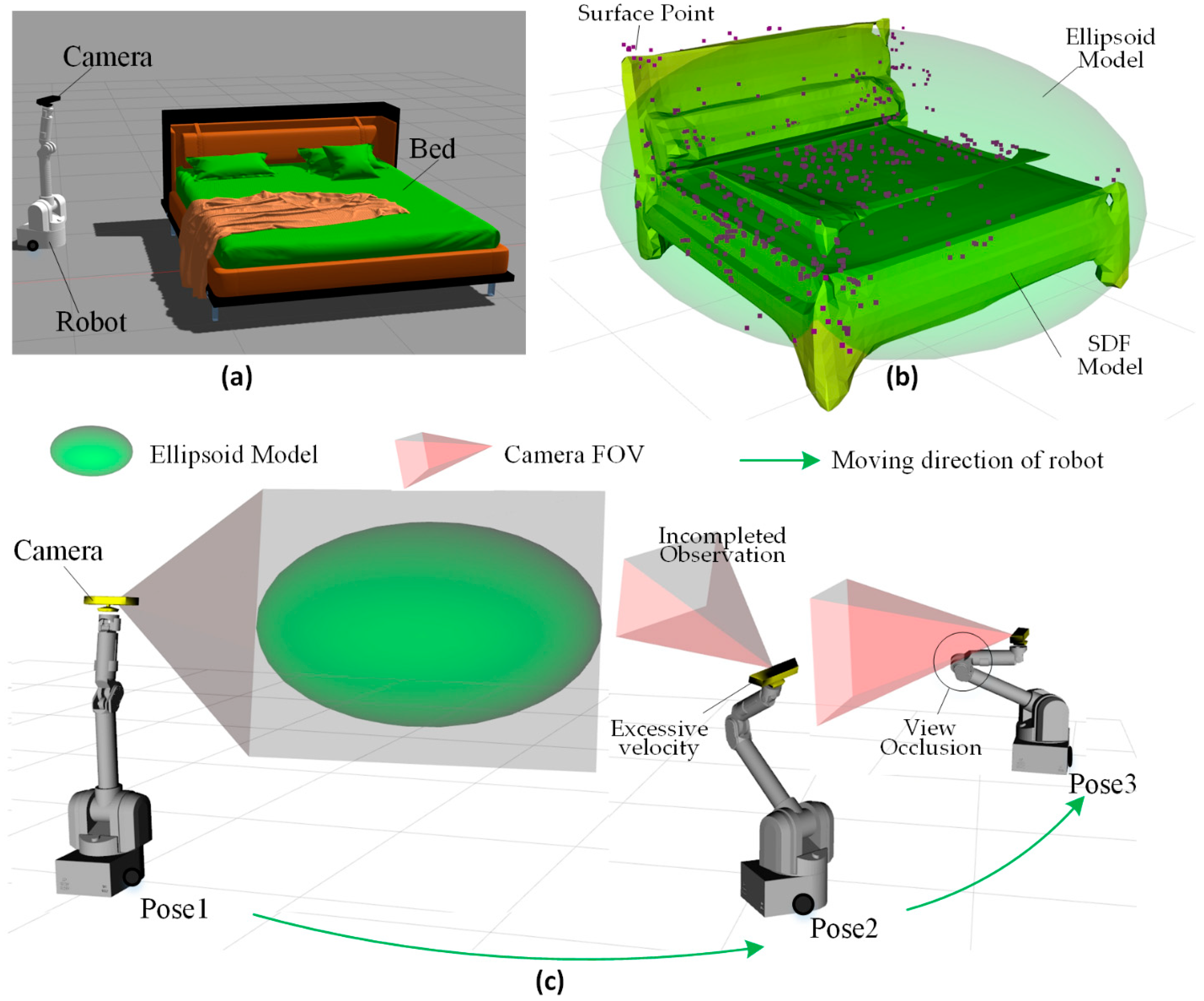
Figure 2.
Factor graph of observation pose optimization.
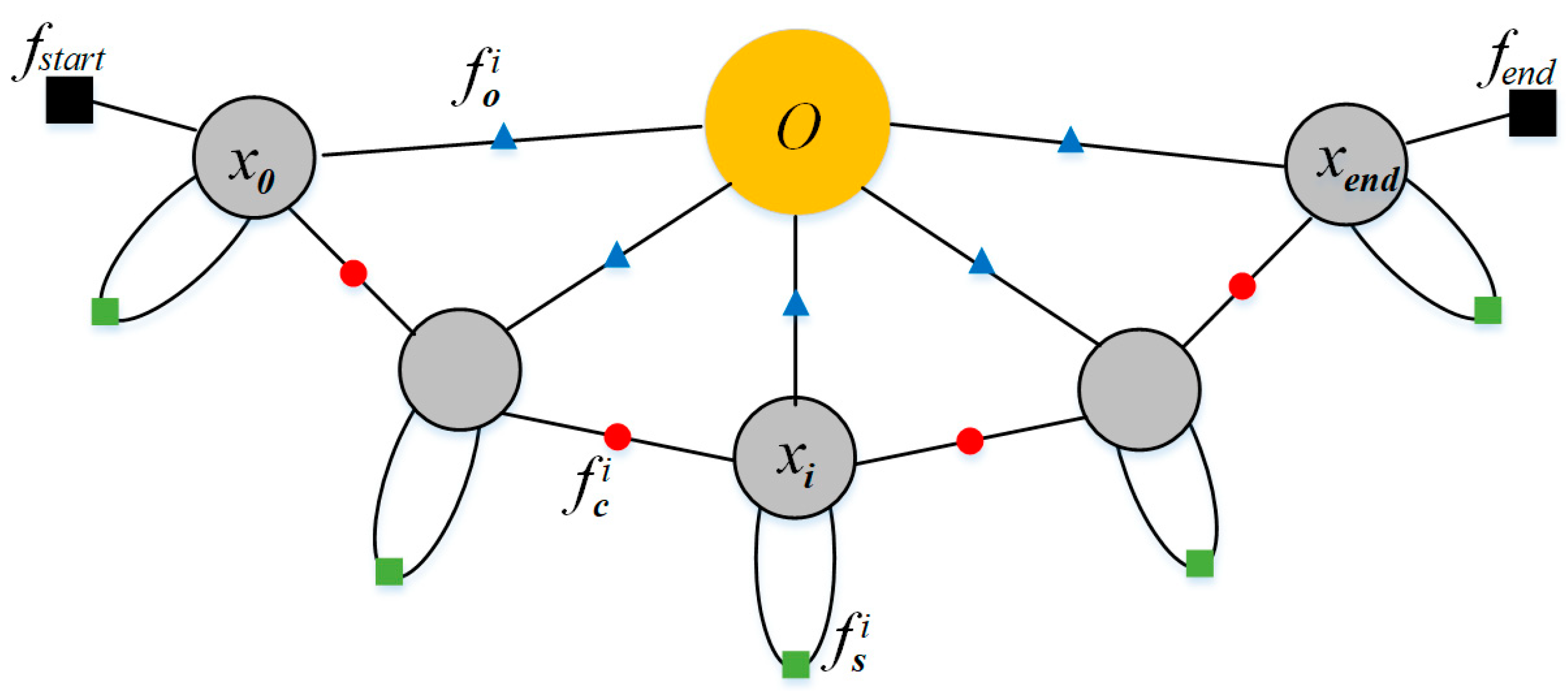
Figure 3.
The Importance and Requirements of Complete Observation. (a) Object model with missing parts; (b) Observation at a too close distance; (c) Observation at a too far distance.Green points represent 3D feature points. Light red mask represents the object segmentation result. If a feature point does not fall within the mask, it is not considered a surface point of the object.
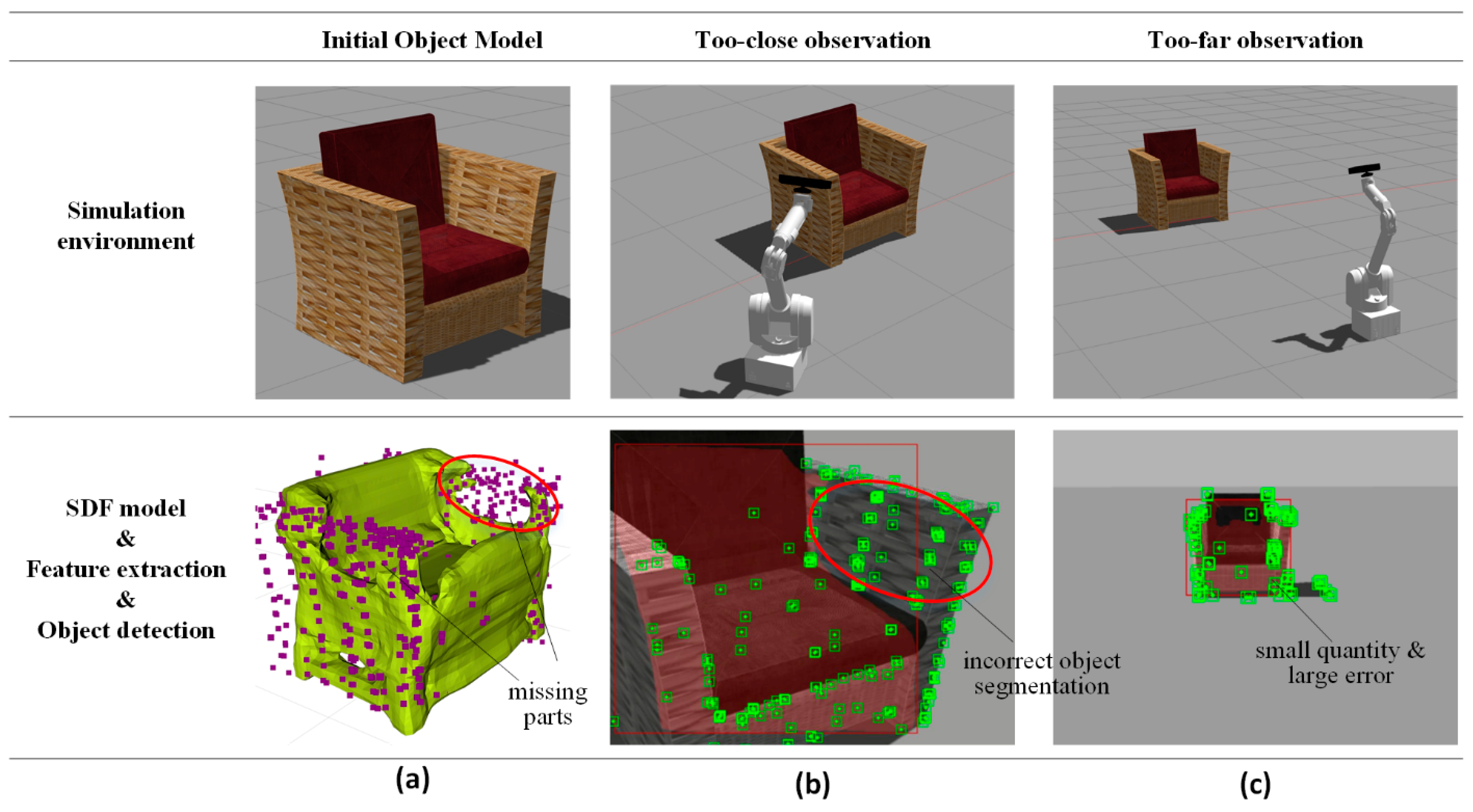
Figure 4.
Definition of the complete object observation: The object model is tangent to the four planes of the camera FOV.
Figure 4.
Definition of the complete object observation: The object model is tangent to the four planes of the camera FOV.
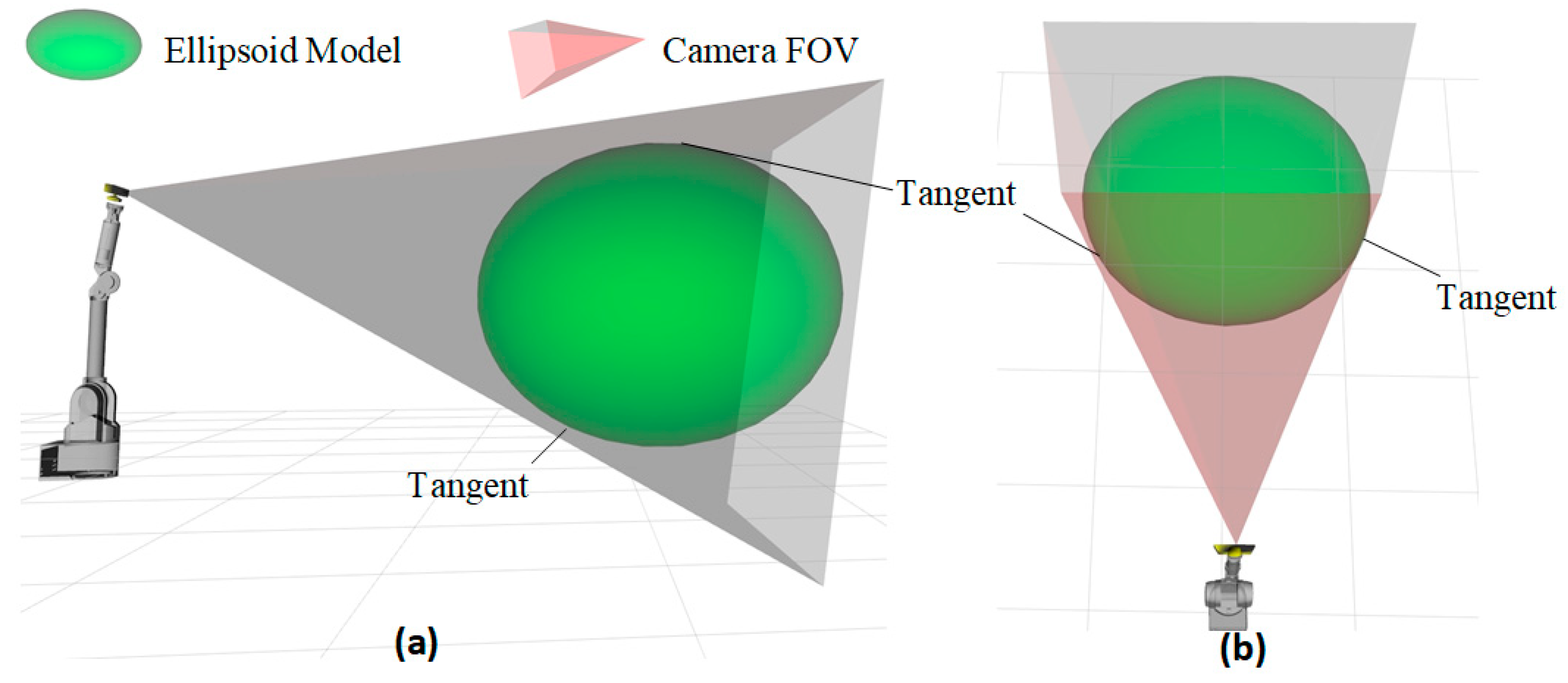
Figure 5.
Projection from Camera Coordinate System to Image Coordinate System. The projections of the four FOV planes form the FOV box, and the ellipsoid is projected into an ellipse.
Figure 5.
Projection from Camera Coordinate System to Image Coordinate System. The projections of the four FOV planes form the FOV box, and the ellipsoid is projected into an ellipse.
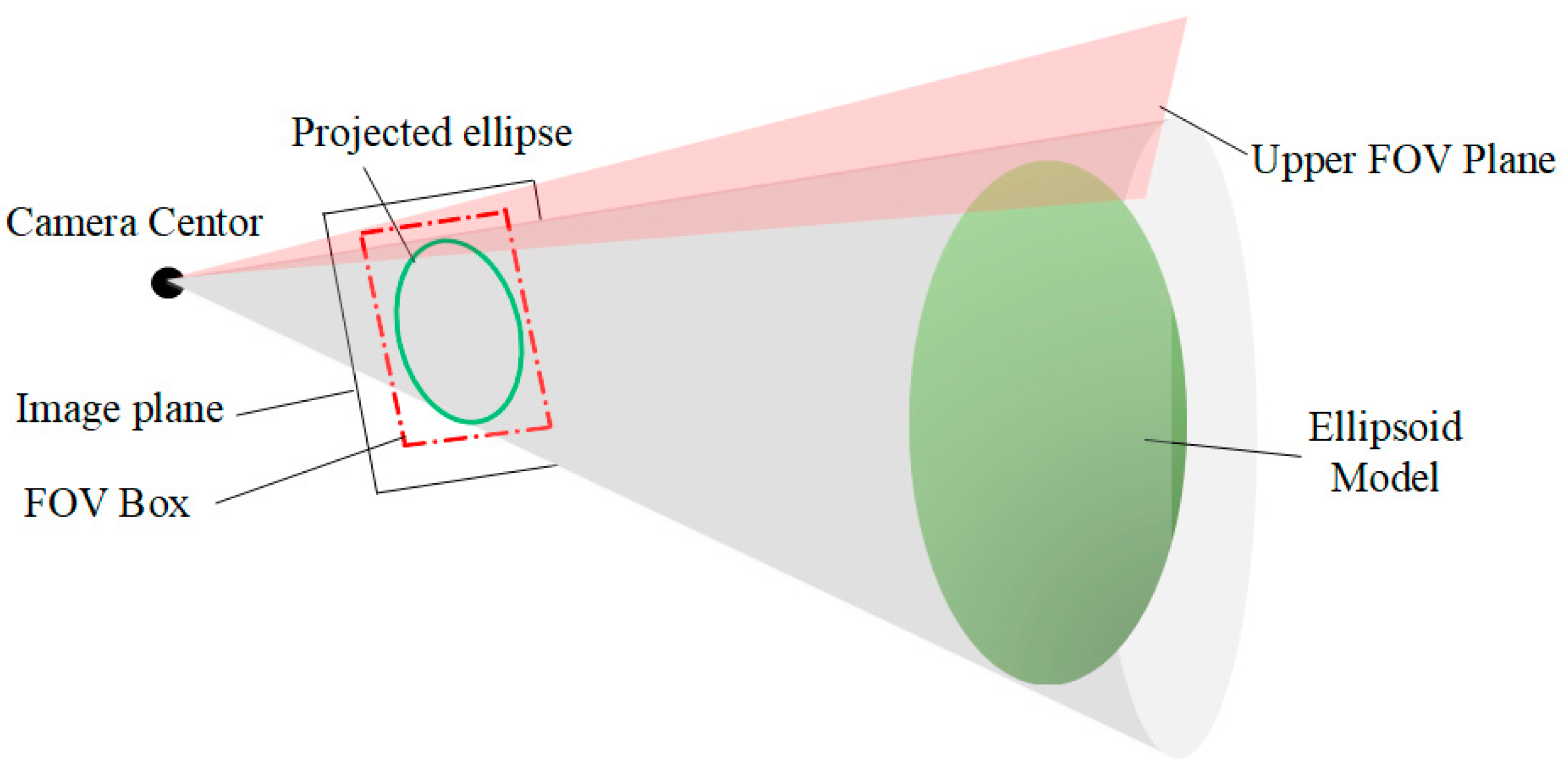
Figure 6.
The deviation between the ellipsoid’s projected bounding box and the FOV box. (a) large deviation, (b) small deviation.
Figure 6.
The deviation between the ellipsoid’s projected bounding box and the FOV box. (a) large deviation, (b) small deviation.
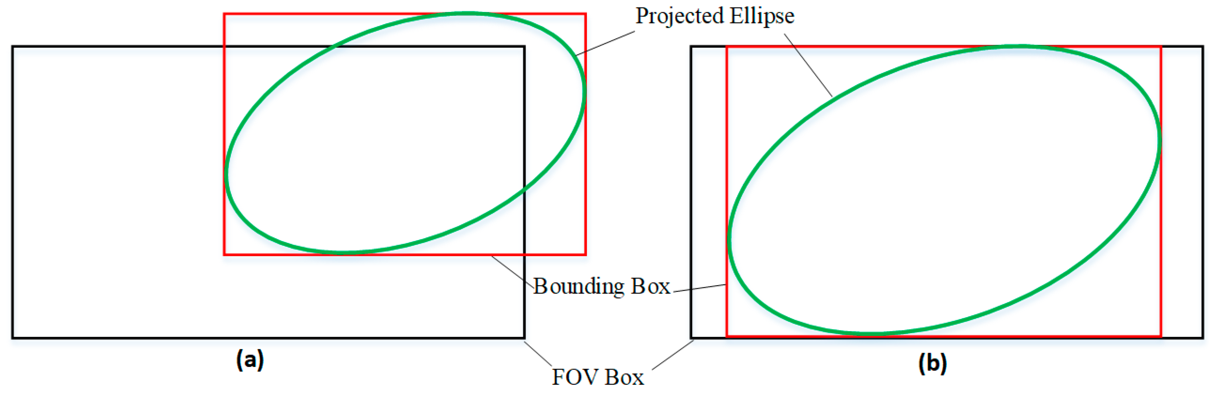
Figure 7.
Concept of Self-Observation Prevention Construction. The yellow entity represents any part of the robotic platform. The FOV needs to avoid the yellow entity.
Figure 7.
Concept of Self-Observation Prevention Construction. The yellow entity represents any part of the robotic platform. The FOV needs to avoid the yellow entity.
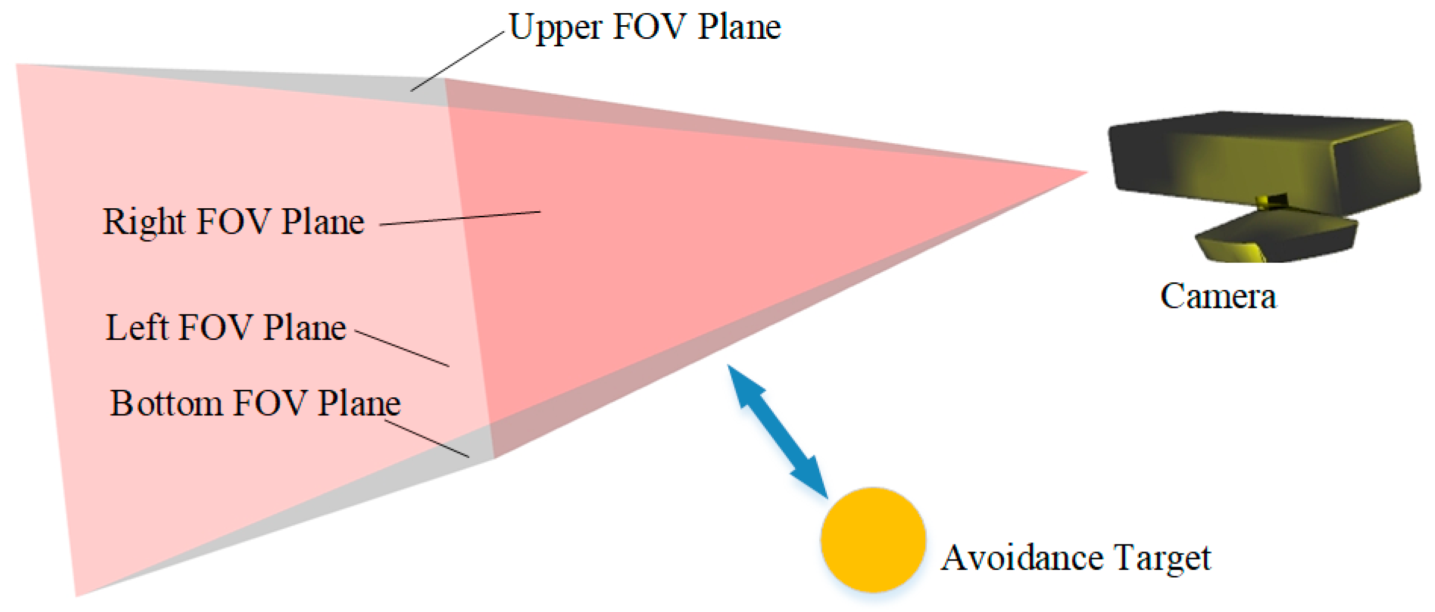
Figure 8.
Avoidance Sphere Coordinate Calculation Based on Robot Kinematics.
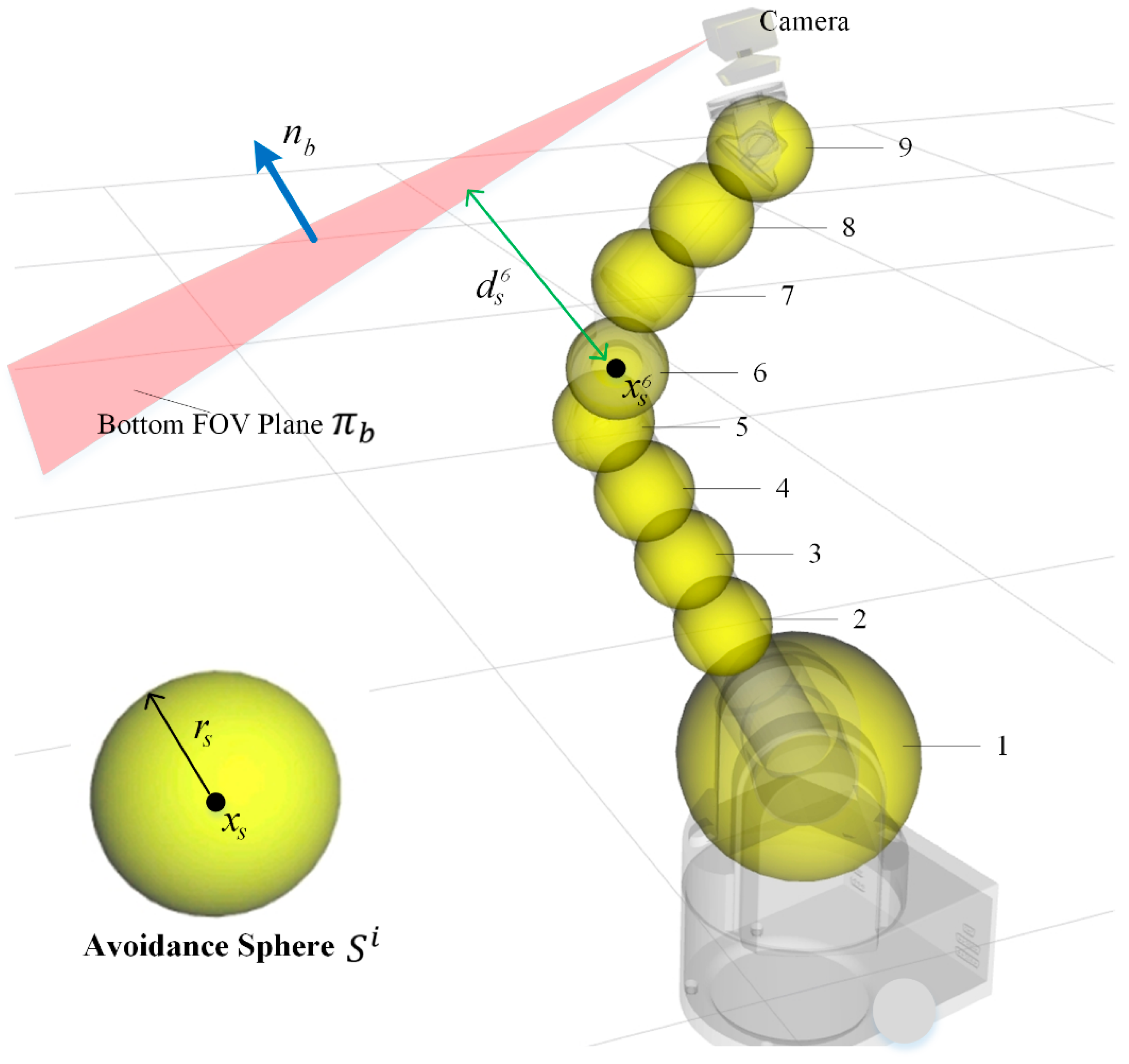
Figure 9.
The trade-off between efficiency and camera motion smoothness. (a)-(d) have large step movements and high efficiency but poor camera smoothness, (a)(e)(f)(g)(d) have small step movements and high camera smoothness but low efficiency.
Figure 9.
The trade-off between efficiency and camera motion smoothness. (a)-(d) have large step movements and high efficiency but poor camera smoothness, (a)(e)(f)(g)(d) have small step movements and high camera smoothness but low efficiency.
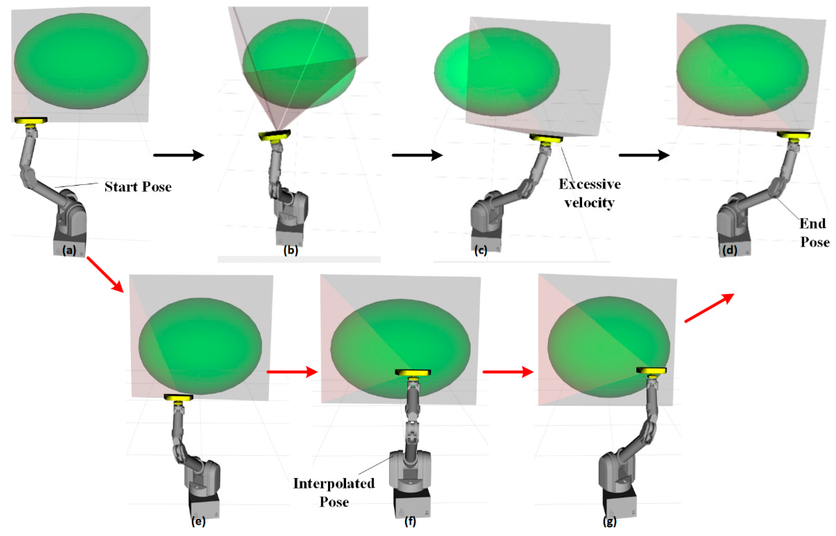
Figure 10.
Object Active SLAM system.
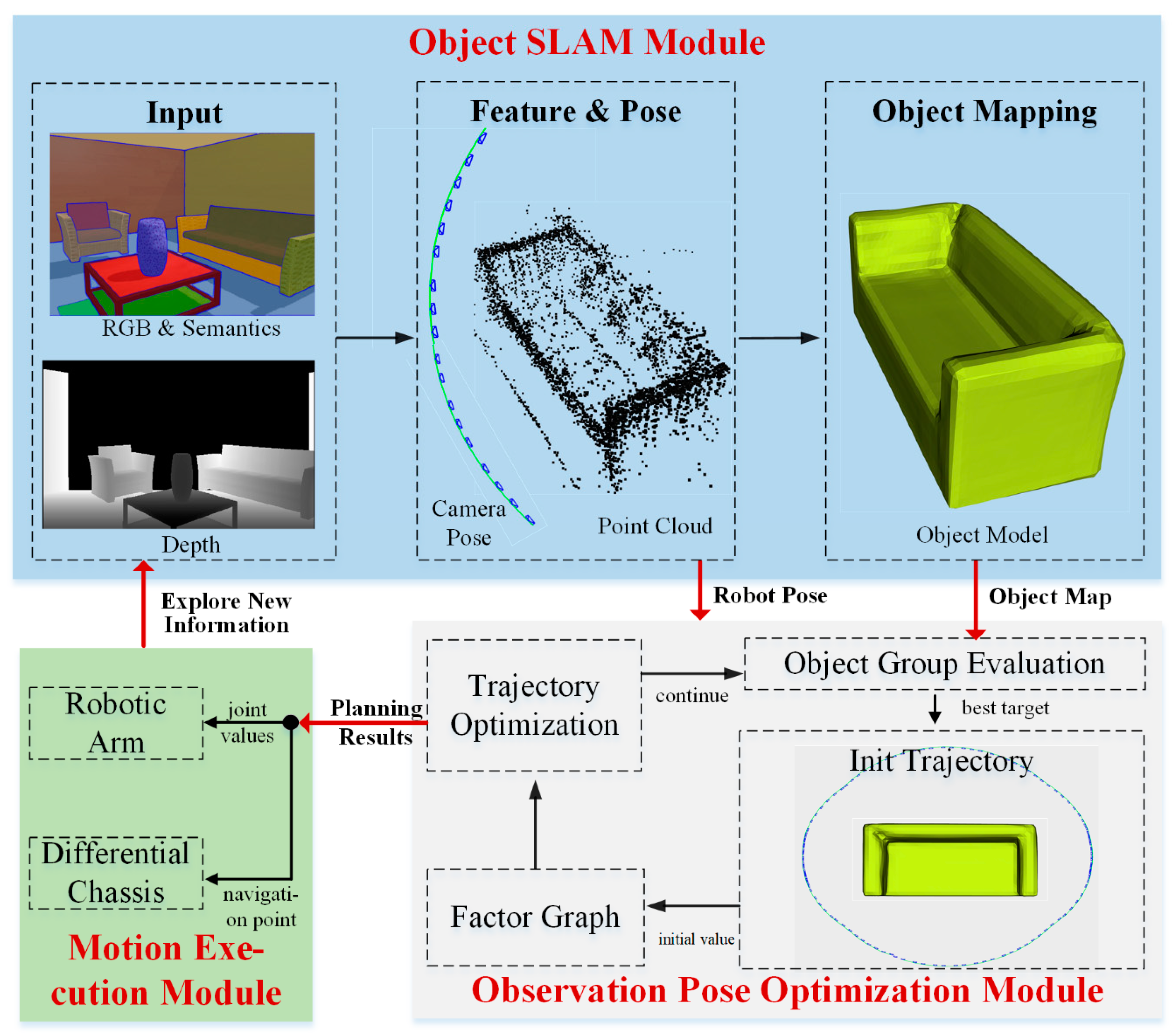
Figure 11.
Experimental environments and robot platform.

Figure 12.
Results of object map and observation trajectory.
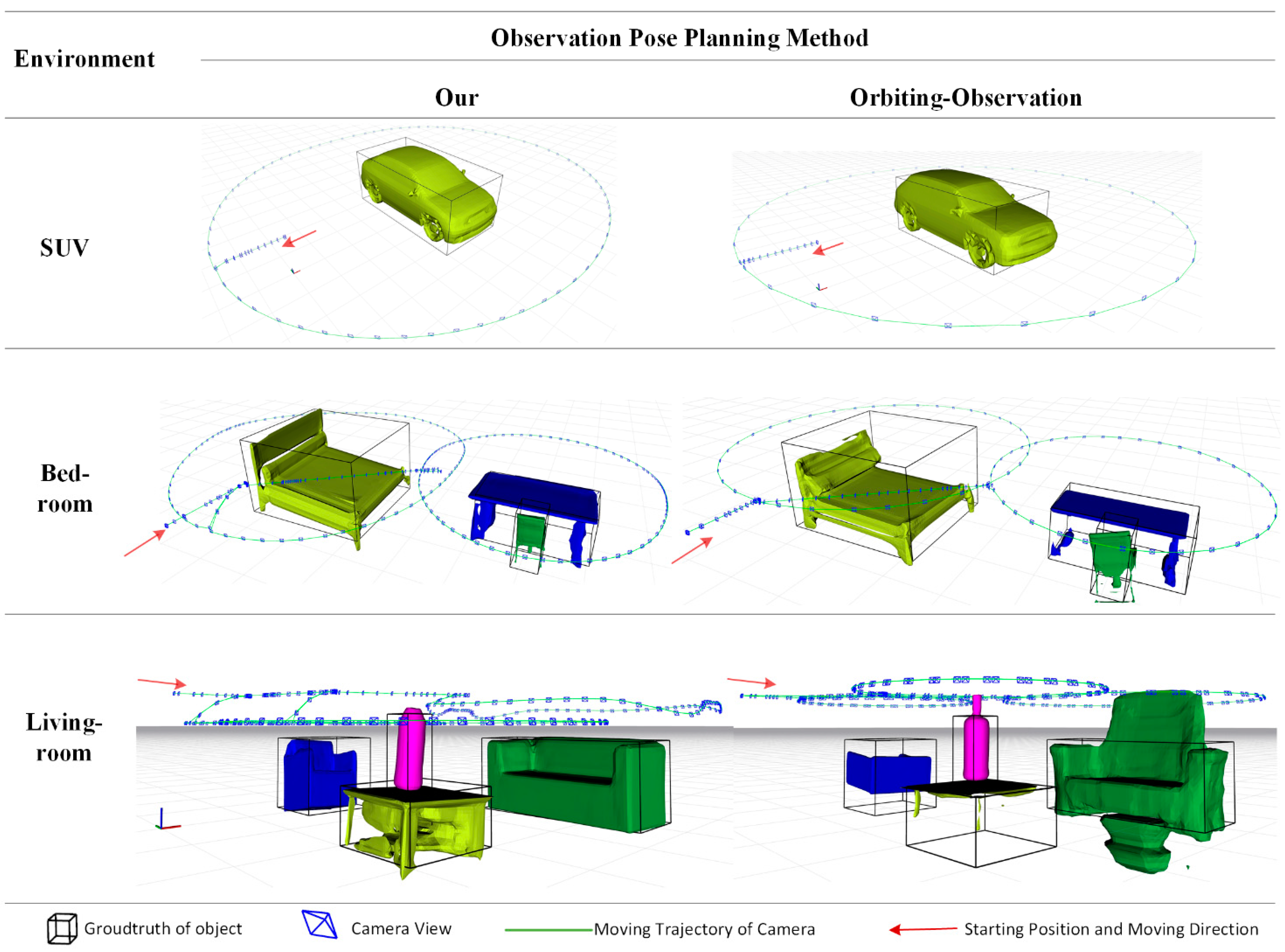
Figure 13.
Comparison of estimated trajectories and the Ground Truth.
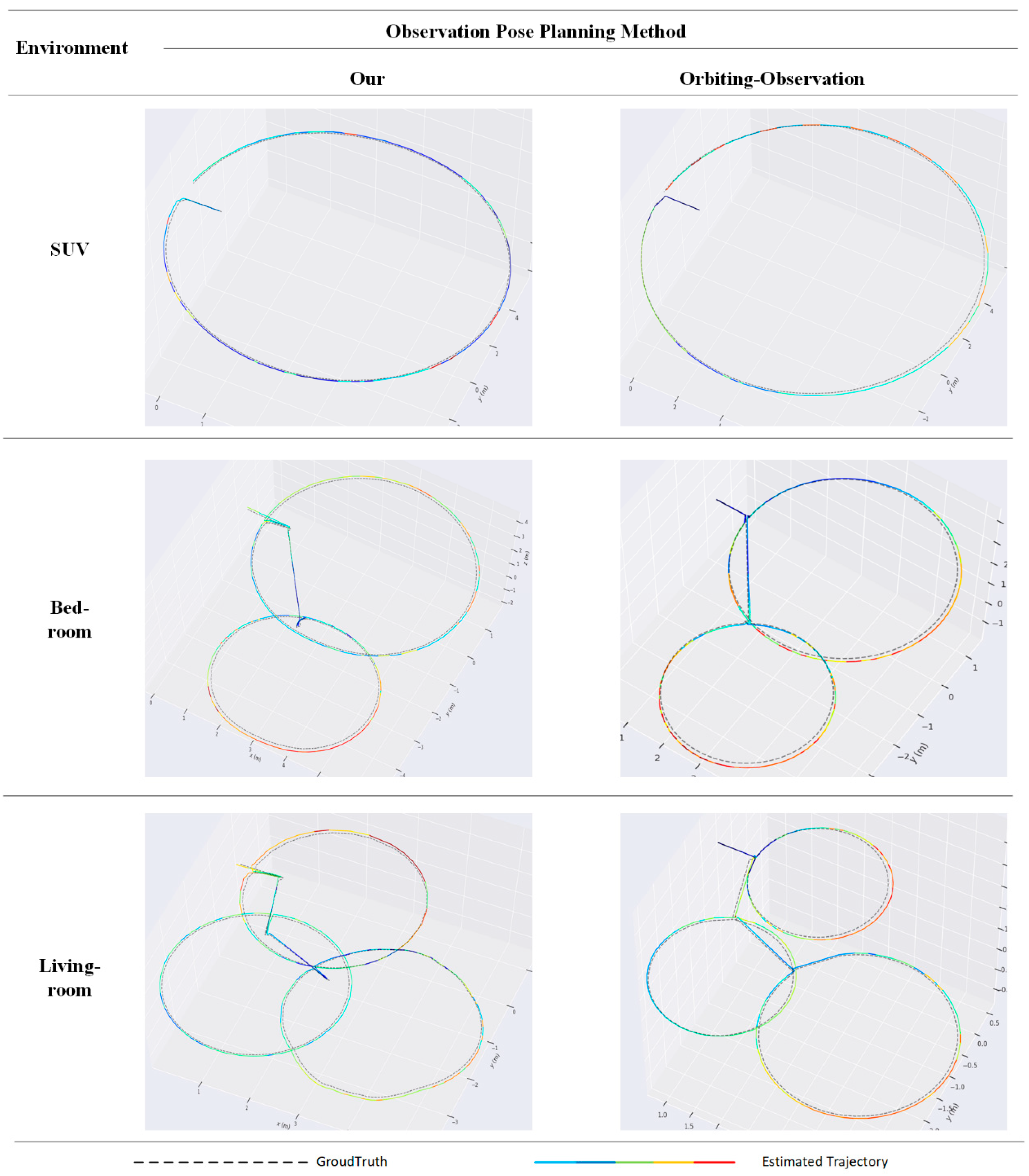

Table 1.
Comparison of Object Modeling Performance.
| Scene | Metrics | Our | Orbiting |
|---|---|---|---|
| SUV | IoU | 0.795 | 0.758 |
| Trans | 0.141 | 0.314 | |
| Rot | 7.3 | 17.2 | |
| Bed-room | IoU | 0.769 | 0.649 |
| Trans | 0.189 | 0.327 | |
| Rot | 9.9 | 36.4 | |
| Living-room | IoU | 0.694 | 0.502 |
| Trans | 0.152 | 0.362 | |
| Rot | 8.9 | 30.1 | |
| Ave | IoU | 0.753 | 0.636 |
| Trans | 0.161 | 0.334 | |
| Rot | 8.7 | 27.9 |
Table 2.
Travel Distance and Motion Time. The Motion Time of our method is recorded as Planning Time + Execution Time.
Table 2.
Travel Distance and Motion Time. The Motion Time of our method is recorded as Planning Time + Execution Time.
| Scene | Metrics | Our | Orbiting |
|---|---|---|---|
| SUV | Length of Chasis Path | 40.7893 | 43.048 |
| Motion Time | 5.3 + 109 | 170 | |
| Bed-room | Length of Chasis Path | 18.4859 | 20.741 |
| Motion Time | 9.2 + 330 | 487 | |
| Living-room | Length of Chasis Path | 27.4061 | 31.4954 |
| Motion Time | 14.8 + 431 | 672 | |
| Ave | Length of Chasis Path | 28.8938 | 31.7615 |
| Motion Time | 9.8 + 290 | 443 |
Table 3.
RMSE of SLAM.
| Scene | Our | Orbiting |
|---|---|---|
| SUV | 0.105279 | 0.110965 |
| Bed-room | 0.074610 | 0.086051 |
| Living-room | 0.074924 | 0.093292 |
| Ave | 0.08494 | 0.09677 |
Disclaimer/Publisher’s Note: The statements, opinions and data contained in all publications are solely those of the individual author(s) and contributor(s) and not of MDPI and/or the editor(s). MDPI and/or the editor(s) disclaim responsibility for any injury to people or property resulting from any ideas, methods, instructions or products referred to in the content. |
© 2025 by the authors. Licensee MDPI, Basel, Switzerland. This article is an open access article distributed under the terms and conditions of the Creative Commons Attribution (CC BY) license (http://creativecommons.org/licenses/by/4.0/).
Copyright: This open access article is published under a Creative Commons CC BY 4.0 license, which permit the free download, distribution, and reuse, provided that the author and preprint are cited in any reuse.


