Submitted:
07 March 2025
Posted:
10 March 2025
You are already at the latest version
Abstract
Missing values pose a challenge in predictive analysis specially in big data because most models depend on complete datasets to estimate functional relationships between variables. Generative Adversarial Imputation Networks are among the most reliable methods to impute missing values with plausible numbers from the dataset. This research introduces Enhanced Generative Adversarial Networks (EGAIN), which address the GAIN convergence issue, introduce new functionality to the GAIN process, and significantly improve its performance.
Keywords:
Missing value
; Imputation
; Generative Adversarial Networks
; Missing completely at random
1. Introduction
Missing values are a common issue in predictive analysis, as most models require complete data to estimate functional relationships among existing variables. There are two main approaches to address missing values in datasets: (1) case deletion, where an entire row of data is removed if it contains at least one missing value, and (2) missing value imputation, where plausible values are estimated and filled in for the missing data. Each method has its drawbacks. Case deletion can significantly reduce the number of samples for predictive analysis, particularly in datasets with a high proportion of missing values, thereby reducing the power of estimations. On the other hand, imputing missing values allows partial information from rows with missing values to be used but may lead to biased results if improper imputations are applied.
Moreover, there are three types of missing values: Missing Completely At Random (MCAR), Missing At Random (MAR), and Missing Not At Random (MNAR) [1]. In MCAR, data is missing purely by chance, e.g., when a survey response is lost because the respondent did not see the question. In this scenario, the missingness is not related to any observed or unobserved data. MAR occurs when the missingness is related to some observed data but not the missing values themselves, e.g., older participants are more likely to skip an income question. In this case, the missing data can be accounted for by other known variables, such as age. MNAR arises when the reason for missingness depends on the unobserved missing data itself, e.g., people with high incomes may choose to hide their salary, resulting in missing income information.
There are many imputation methods that reliably handle different types of missing data. Among them is Multiple Imputation by Chained Equations (MICE), which predicts missing values using an iterative process and regression of observed variables on the missing ones [2]. While MICE is well-suited for datasets with mixed numerical and categorical variables and preserves relationships between variables, its iterative process is time-consuming. Moreover, it may fail to properly impute missing values when non-linear relationships exist between variables [3]. MissForest is another common missing value imputation technique that uses random forests to predict and fill in missing values [4]. This method is effective for handling complex datasets with both numerical and categorical variables and captures non-linear relationships between variables. However, MissForest is highly time-consuming, especially for large datasets. Its performance drops significantly when a large portion of the data is missing and may introduce bias in datasets with extreme values or skewed distributions [5].
Generative Adversarial Imputation Networks (GAIN) is a deep learning-based approach for missing value imputation that models the distribution of observed data to impute missing values [6]. GAIN handles both numerical and categorical variables and performs well even when the data distribution is imbalanced or skewed [7]. However, it is sensitive to hyperparameter selection, and suffers from encoding issues and reduced accuracy for multi-class variables. For a comprehensive review of models for handling missing data, see [8].
Several researchers have provided performance comparisons between MICE, MissForest, and GAIN on benchmark datasets [7,9,10]. The results indicate that the performance of these models depends heavily on factors such as the type (numerical/categorical) and number of variables, variable skewness, number of cases, the percentage and type of missing values. GAIN has demonstrated superior performance over MICE and MissForest in many areas, including speed and handling high missing rates.
Several variations of GAIN have been proposed since its introduction in 2018. Among them are: LFM-D2GAIN, which integrates a latent factor model (LFM) for coherent training and reduced reconstruction error, along with a dual-discriminator (D2) to capture multi-modal data distribution [11]; GAGIN, which integrates global and local imputation networks with an imputation guider model to address local homogeneity and improve prediction performance [12]; ClueGAIN, which incorporates transfer learning to improve imputation accuracy in datasets with high missing rates [13]; ccGAIN, which enhances imputation accuracy by conditioning imputation on observed and annotated values in clinical data with high missing rates [14]; LWGAIN, which integrates the Wasserstein distance in the loss function and incorporates labeled inputs into the generator, improving imputation performance on the Kansas logging dataset and enabling effective lithology identification [15].
Despite the many variations built on GAIN, its application still relies on the outdated TensorFlow 1.x Application Programming Interface (API) and several nonstandard user-defined functions for scaling, sampling, and network initiation. Moreover, its deep networks that are considered the center of the process are simple deep neural networks, unable to discover the spatial relationships in the input data. Crucially, GAIN implementation is very sensitive to the choice of hyperparameters and often exhibits convergence issues, especially when missing data is limited to a small number of variables, a characteristic prevalent in most real-life datasets. Indeed, Sun et al. (2023) highlight the lack of standardized software for the GAIN method.
We introduce Enhanced Generative Adversarial Networks (EGAIN), which address the GAIN convergence issue, introduce new functionality to the GAIN process, and significantly improve its performance. The enhancements are discussed in detail in the following section. The EGAIN codes, along with instructions on how to use them and sample runs, will be provided as a Python 3.x package on https://github.com.
2. Materials and Methods
The Generative Adversarial Imputation Network (GAIN) introduced by Yoon et al. (2018) formulates imputation of missing values as a learning problem, leveraging a generator (G) and discriminator (D) in a competitive setting inspired by Generative Adversarial Networks (GANs). The core idea of GAIN is to generate plausible imputations for missing values using a generator, denoted as
where is the data array whose missing values are replaced with zero, M is the binary mask array whose values are 1 for observed data, and 0 for missing, and Z is random noise applied only to missing value arrays. Once the generator imputes the missing values, the discriminator (D) attempts to distinguish real values from imputed ones by outputting a probability array that indicates the chance of each component being real, using:
where is the output of the generator, and H is the hint array that provides partial information about which values are missing. The generator and discriminator networks are trained over a large number of iterations, while improving their performance by reducing competing loss functions. The discriminator is trained to maximize classification (real/imputed) accuracy by minimizing the following binary cross entropy loss function:
The generator is trained to minimize the discriminator’s ability to differentiate real values from imputed ones, with the following loss function:
This loss function is only applied to imputed missing and penalizes G if D performs well by correctly outputting low chances. To encourage the generator to produce realistic values that deceive the discriminator, a reconstruction loss is added to the generator:
This loss function is only applied to observed values . Therefore, the total generator loss becomes:
where is a hyperparameter that controls the contribution of the reconstruction loss to the overall objective. The competition between the generator and the discriminator drives the generator to produce high-quality imputations that are indistinguishable from real data. It is important to note that only the continuous reconstruction loss has been used in the GAIN implementation and its successors.
The following are a series of enhancements that has been applied to the GAIN implementation, driving the EGAIN with improved performance:
- GAIN algorithm has been implemented using tf.compat.v1, which is part of the TensorFlow 1.x API that is intended to aid migration from TF1 to TF2 [16]. EGAIN, on the other hand, is implemented in TensorFlow 2, benefiting from improved performance optimizations, reduced boilerplate code, enhanced function tracing, and increased readability, debuggability, and maintainability.
- GAIN algorithm utilizes a deep neural network for both the generator and the discriminator, each composed of two dense layers. The data with missing values and its corresponding mask array are concatenated side by side (by columns) before being fed into the networks. EGAIN, on the other hand, employs a deep convolutional neural network for the generator and the discriminator, consisting of one convolutional layer followed by a max-pooling layer, along with two dense layers. In this approach, the data with missing values and its mask array are stacked on top of each other, similar to a sandwich, before being fed into the network. This structure enables the network to capture spatial associations in the input more effectively.
- GAIN implementation is highly sensitive to hyperparameter selection and may fail to converge or produce results if the number of iterations is not appropriate. This issue is particularly evident when missing values exist in only a few columns, as seen in MAR and MNAR scenarios. In contrast, EGAIN consistently provides reliable imputations in every run. This is accomplished through the use of checkpoints, where the network weights are stored and recalled when performance issues arise.
- GAIN implementation includes several nonstandard user-defined functions for scaling, sampling, and network initialization, whereas EGAIN utilizes standard built-in functions. For example, Xavier initialization is implemented as a user-defined function in GAIN for network weight initialization, while EGAIN leverages the built-in Xavier initialization for layer kernels.
- EGAIN provides charts displaying the loss function over iterations, aiding in hyperparameter selection and offering a visual indication of network performance. In contrast, GAIN lacks such a chart and since it is highly sensitive to hyperparameters, the network often fails to converge when poor hyperparameter choices are made.
Table 1 summarizes the benchmark UCI datasets [17] that are used to assess the performance of the EGAIN model compared to the GAIN [6]. For each dataset, different missingness settings are considered with a range of missing value rates. MCAR missing values are generated using standard functions based on Rubin (1976). After introducing missing values into complete datasets, GAIN and EGAIN were used for imputation, and their performance was evaluated using Root Mean Squared Error (RMSE):
where n is the number of missing values, is real value from completed data, and is the imputed missing value. Min/Max scaling is applied prior to calculation of performance metrics so that all variables have the same range of values. Experiments were conducted 25 times independently. A hint rate of 90% was used for all imputations. A batch size of 64 was employed for small and medium datasets, while 256 was used for large datasets. The hyperparameter was selected by observing the generator and discriminator loss functions to ensure they began at approximately the same value (see Figure 2). Line charts display the average and standard deviation of performance metrics across 25 runs. Details of these runs and their hyperparameters are provided in the supplementary materials.
3. Results
Figure 1 shows a performance comparison of GAIN and EGAIN on the breast cancer dataset for (a) missing values selected completely at random from the 30 numerical predictors at various rates. The results indicate a significant () RMSE reduction of 5.37% to 18.74% for EGAIN compared to GAIN. More importantly, the convergence of the GAIN implementation was highly dependent on the number of iterations, often failing to generate results when the number of iterations exceeded an optimal threshold. As a result, different numbers of iterations were used for different missing rates (see supplementary run data). In contrast, the EGAIN implementation produced results regardless of the number of iterations, with performance improving as the number of iterations increased.
The issue with the GAIN implementation becomes more evident when missing values are present in only a few columns, which is common in real-world datasets. In Figure 1(b), missing values at various rates were selected completely at random from a subset of randomly chosen columns among the 30 numerical predictors. EGAIN demonstrates significant () performance improvements ranging from 5.25% (16 random columns with 75% total missing) to 46.22% (2 random columns with 50% total missing). Notably, the GAIN implementation failed to produce results more frequently as the number of iterations increased. Consequently, different numbers of iterations were used for each setting. For a complete list of results and details on hyperparameter choices, please refer to the supplementary materials.
Figure 2, generated using EGAIN, illustrates the discriminator and generator loss functions throughout the training iterations. It is evident that both the discriminator and generator improve their performance over iterations, as indicated by the decreasing loss values. The loss begins to increase slightly shortly after iteration 10 as the discriminator improves its performance, which in turn penalizes the generator, forcing it to produce more realistic imputations. This chart can be used to select the value of such that the initial loss values of the discriminator and generator are nearly equal. In this example, was chosen. Although the number of iterations was set to 1000, the minimum generator loss was observed around iteration 520. EGAIN effectively stores the network weights at this iteration using checkpoints and utilizes them to generate the final imputation. This functionality is absent in GAIN, making it susceptible to overtraining, which ultimately leads to failure in imputing missing values. The discriminator loss is multiplied by 10 in the EGAIN implementation to penalize the discriminator more severely and to produce more consistent plots. EGAIN can also resume training from its stored checkpoint weights, improving upon the results of the previous runs.
Figure 2.
Progress of the loss functions throughout training in breast cancer data.
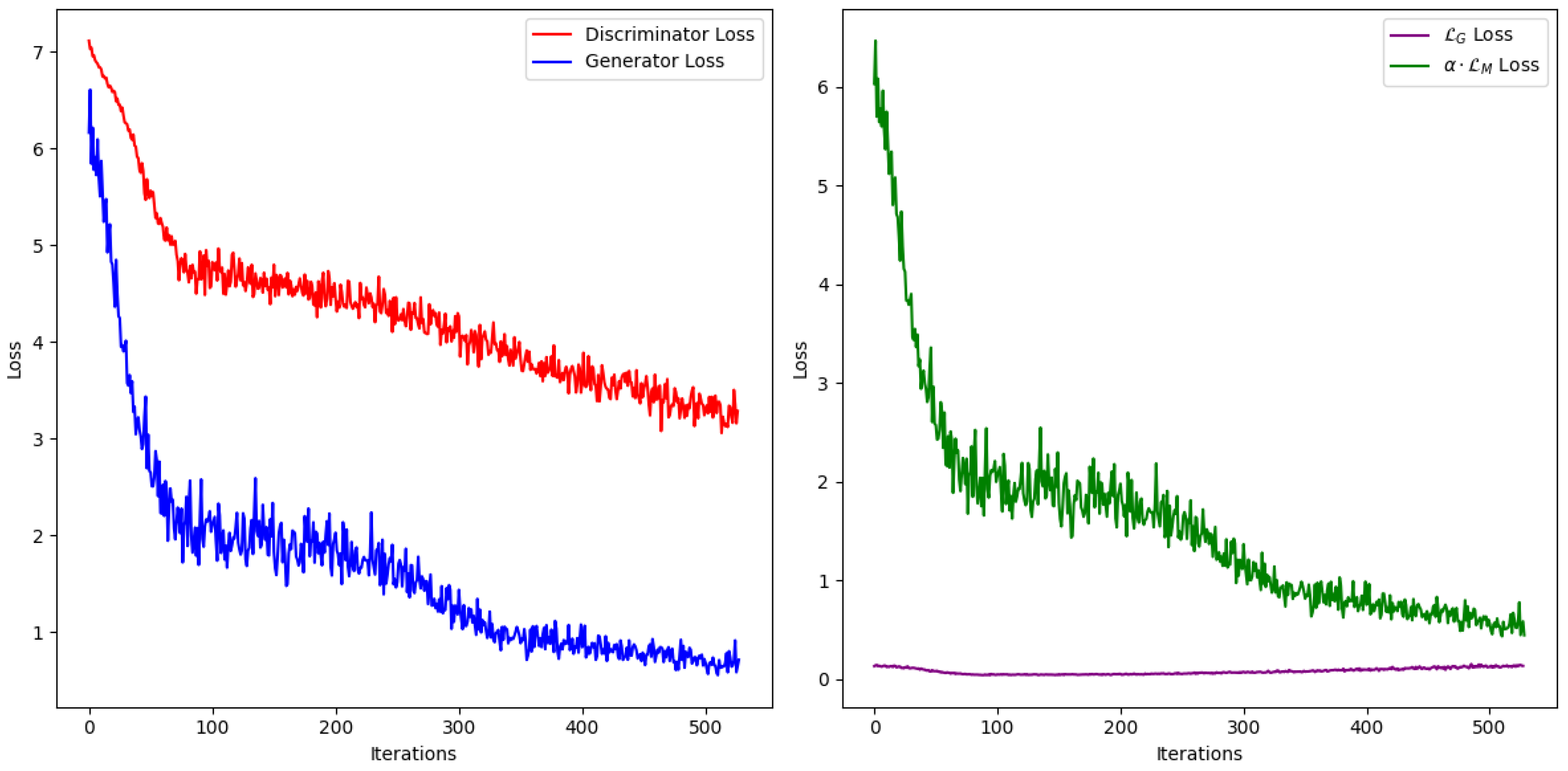
Figure 3 shows a performance comparison of GAIN and EGAIN on the spam dataset for (a) missing values selected completely at random from the 57 numerical predictors at various rates. EGAIN illustrates improved performance compared to GAIN in all missing rates. A two factor ANOVA reveals a significant difference () in perfromance between GAIN and EGAIN. The diference in performance was more evident when (b) missing values were selected from a subset of randomly chosen columns among the 57 features at various rates. Once again, GAIN often failed to generate results when the number of iterations exceeded an optimal selected threshold.
Performance comparisons between GAIN and EGAIN in credit dataset are shown in Figure 4. EGAIN illustrates significant performance improvement () compared to GAIN across different missing value rates. Note that GAIN was very sensitive to the choice of training iterations and failed to provide imputations passed the selected iterations in the study; see supplementary data.
Table 2 summarizes the overall imputation performance across the discussed experiments. EGAIN has demonstrated a significant performance improvement compared to GAIN across small, medium, and large datasets, reducing the RMSE by 3.21%, 24.77%, and 19.73% in the breast cancer, spam, and credit datasets, respectively. Notably, the most significant achievement of EGAIN is its ability to resolve GAIN’s convergence issue; see the supplementary data for details.
4. Discussion
MICE, MissForest, and GAIN are among the most common methods for imputing missing values in a dataet. GAIN outperforms MICE and MissForest by capturing complex data distributions, handling high missing rates, and learning implicit patterns without assuming specific distributions. It scales better to large datasets, provides more consistent imputations through adversarial training, and adapts well to different data types. Despite the many variations built on GAIN, its implementation still relies on the outdated TensorFlow 1.x API, uses several nonstandard user-defined functions, and requires careful hyperparameter tuning. EGAIN, introduced in this paper, is built on the TensorFlow 2 API, resolves the convergence issues of GAIN using checkpoint saving, and provides visualizations of loss functions to aid in hyperparameter selection. Results show that EGAIN outperforms GAIN in terms of RMSE across several benchmark datasets.
Regarding computational time, EGAIN exhibits a runtime approximately three to four times longer than GAIN. Specifically, imputing 20% missing values in a credit dataset containing 30,000 cases requires an average of 20 seconds for EGAIN, utilizing 1000 iterations and a batch size of 256. This is primarily due to the use of a convolutional layer in both the generator and discriminator. Although this runtime is manageable for individual imputations, it accumulates substantially during simulations involving hundreds of independent runs. Conversely, GAIN’s average runtime is 5.5 seconds; however, with 1000 iterations, it failed to generate successful imputations, as this exceeds its recommended iteration limit of 500.
This study focused solely on missing value imputation in MCAR scenarios. A follow-up study is required to compare the performance of EGAIN and its alternatives in MAR and MNAR scenarios.
Author Contributions
Methodology, A.Saghafi; Software, A.Saghafi; Validation, A.Saghafi and S.Moallemian and M.Budak and R.Deshpande; Visualization, A.Saghafi and S.Moallemian and M.Budak and R.Deshpande; Supervision, A.Saghafi; writing—original draft preparation, A.Saghafi; writing—review and editing, A.Saghafi and S.Moallemian and M.Budak and R.Deshpande; All authors have read and agreed to the submitted version of the manuscript.
Funding
This research received no external funding.
Data Availability Statement
All data and codes will be publicly available at https://github.com/.
Conflicts of Interest
The authors declare no conflicts of interest.
Abbreviations
The following abbreviations are used in this manuscript:
| GAIN | Generative Adversarial Imputation Network |
| EGAIN | Enhanced Generative Adversarial Imputation Network |
| MAR | Missing At Random |
| MCAR | Missing Completely At Random |
| MNAR | Missing Not At Random |
| MICE | Multiple Imputation by Chained Equations |
| LFM-D2GAIN | Latent Factor Model with Dual Discriminator GAIN |
| GAGIN | Generative Adversarial Guider Imputation Network |
| ccGAIN | Conditional Clinical GAIN |
| LWGAIN | Loss Wasserstein GAIN |
| TensorFlow | TF |
| API | Application Programming Interface |
| RMSE | Root Mean Squared Error |
References
- Rubin, D. Inference and missing data. Biometrika 1976, 63, 581–592. [Google Scholar]
- Van Buuren, S.; Groothuis-Oudshoorn, K. mice: Multivariate Imputation by Chained Equations in R. Journal of Statistical Software 2011, 45, 1–67. [Google Scholar]
- White, I.; Royston, P.; Wood, A. Multiple imputation using chained equations: Issues and guidance for practice. Statistics in Medicine 2011, 30, 377–399. [Google Scholar] [PubMed]
- Stekhoven, D.; Buhlmann, P. MissForest—non-parametric missing value imputation for mixed-type data. Bioinformatics 2011, 28, 112–118. [Google Scholar] [CrossRef] [PubMed]
- Waljee, A.; Mukherjee, A.; Singal, A.; Zhang, Y.; Warren, J.; Balis, U.; Marrero, J.; Zhu, J.; Higgins, P. Comparison of imputation methods for missing laboratory data in medicine. BMJ Open 2013, 3, e002847. [Google Scholar] [CrossRef] [PubMed]
- Yoon, J.; Jordon, J.; Van Der Schaar, M. GAIN: Missing Data Imputation using Generative Adversarial Nets. In Proceedings of the 35th International Conference on Machine Learning, Stockholm, Sweden, 10-15 July 2018. [Google Scholar]
- Dong, W.; Fong, D.; Yoon, J.; Wan, E.; Bedford, L.; Tang, E.; Lam, C. Generative adversarial networks for imputing missing data for big data clinical research. BMC Medical Research Methodology 2021, 21, 78. [Google Scholar]
- Zhou, Y.; Aryal, S.; Bouadjenek, M. Review for Handling Missing Data with special missing mechanism. arXiv 2024. [Google Scholar]
- Sun, Y.; Li, J.; Xu, Y.; Zhang, T.; Wang, X. Deep learning versus conventional methods for missing data imputation: A review and comparative study. Expert Systems with Applications 2023, 227, 120201. [Google Scholar]
- Shahbazian, R.; Greco, S. Generative Adversarial Networks Assist Missing Data Imputation: A Comprehensive Survey and Evaluation. IEEE Access 2023, 11, 88908–88928. [Google Scholar]
- Shen, Y.; Zhang, C.; Zhang, S.; Yan, J.; Bu, F. LFM-D2GAIN: An Improved Missing Data Imputation Method Based on Generative Adversarial Imputation Nets. In Proceedings of the 2022 IEEE International Conference on Electrical Engineering, Big Data and Algorithms (EEBDA), Changchun, China, 25-27 February 2022. [Google Scholar]
- Wang, W.; Chai, Y.; Li, Y. GAGIN: generative adversarial guider imputation network for missing data. Neural Computing and Applications 2022, 34, 7597–7610. [Google Scholar]
- Zhao, S. ClueGAIN: Application of Transfer Learning On Generative Adversarial Imputation Nets (GAIN). arXiv 2023. [Google Scholar]
- Bernardini, M.; Doinychko, A.; Romeo, L.; Frontoni, M.; Amini, M. A novel missing data imputation approach based on clinical conditional Generative Adversarial Networks applied to EHR datasets. Computers in Biology and Medicine 2023, 163, 107188. [Google Scholar]
- Qian, H.; Geng, Y.; Wang, H.; Wu, X.; Li, M. LWGAIN: An Improved Missing Data Imputation Method Based on Generative Adversarial Imputation Network. In Proceedings of the 2024 5th International Conference on Computer Vision, Image and Deep Learning (CVIDL), Zhuhai, China, 19-21 April 2024. [Google Scholar]
- TensorFlow 1.x vs TensorFlow 2 - Behaviors and APIs. Available online: https://www.tensorflow.org/guide/migrate/tf1_vs_tf2 (accessed on Feb, 2025).
- The UCI Machine Learning Repository. Available online: https://archive.ics.uci.edu (accessed on Feb, 2025).
Figure 1.
Performance comparison of GAIN vs EGAIN for breast cancer dataset: (a) MCAR from the 30 columns. (b) MCAR from randomly selected columns among 30 numerical features.
Figure 1.
Performance comparison of GAIN vs EGAIN for breast cancer dataset: (a) MCAR from the 30 columns. (b) MCAR from randomly selected columns among 30 numerical features.
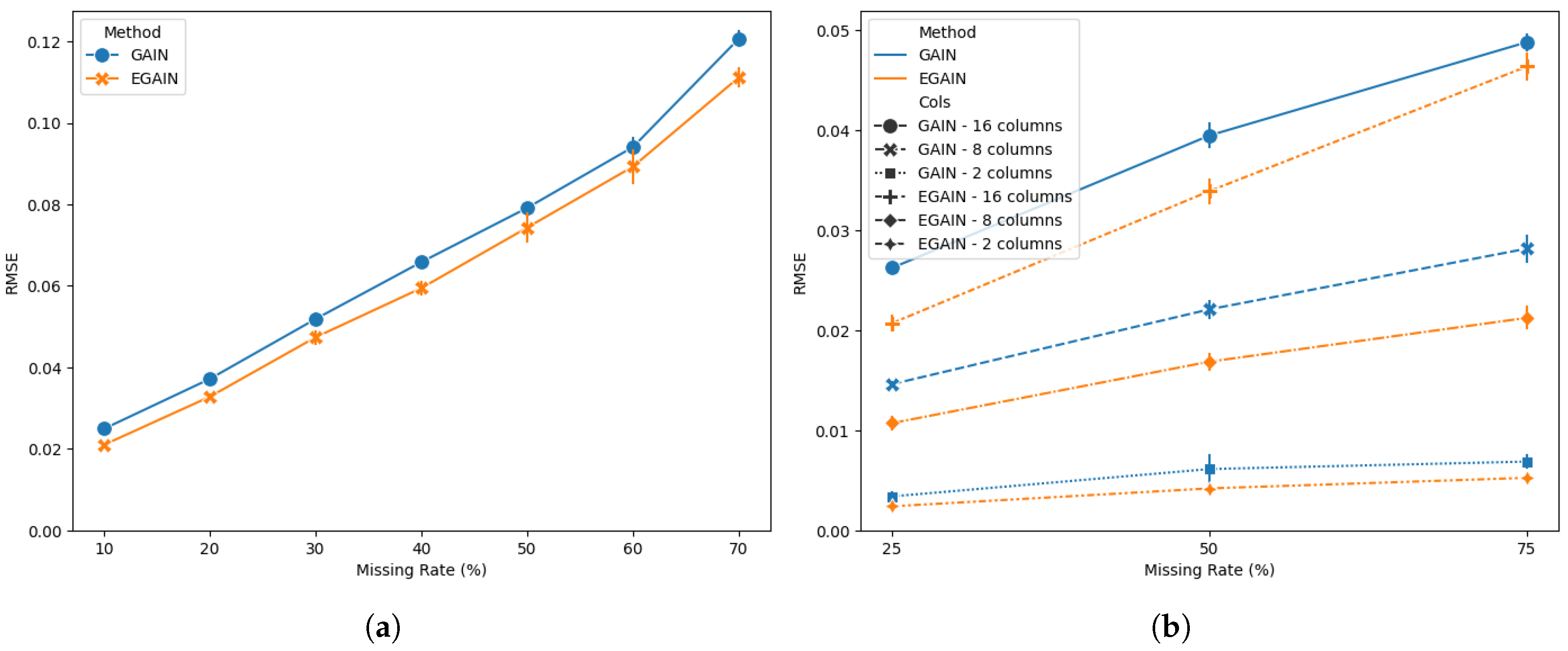
Figure 3.
Performance comparison of GAIN vs EGAIN for spam dataset: (a) MCAR from the 57 columns. (b) MCAR from randomly selected columns.
Figure 3.
Performance comparison of GAIN vs EGAIN for spam dataset: (a) MCAR from the 57 columns. (b) MCAR from randomly selected columns.
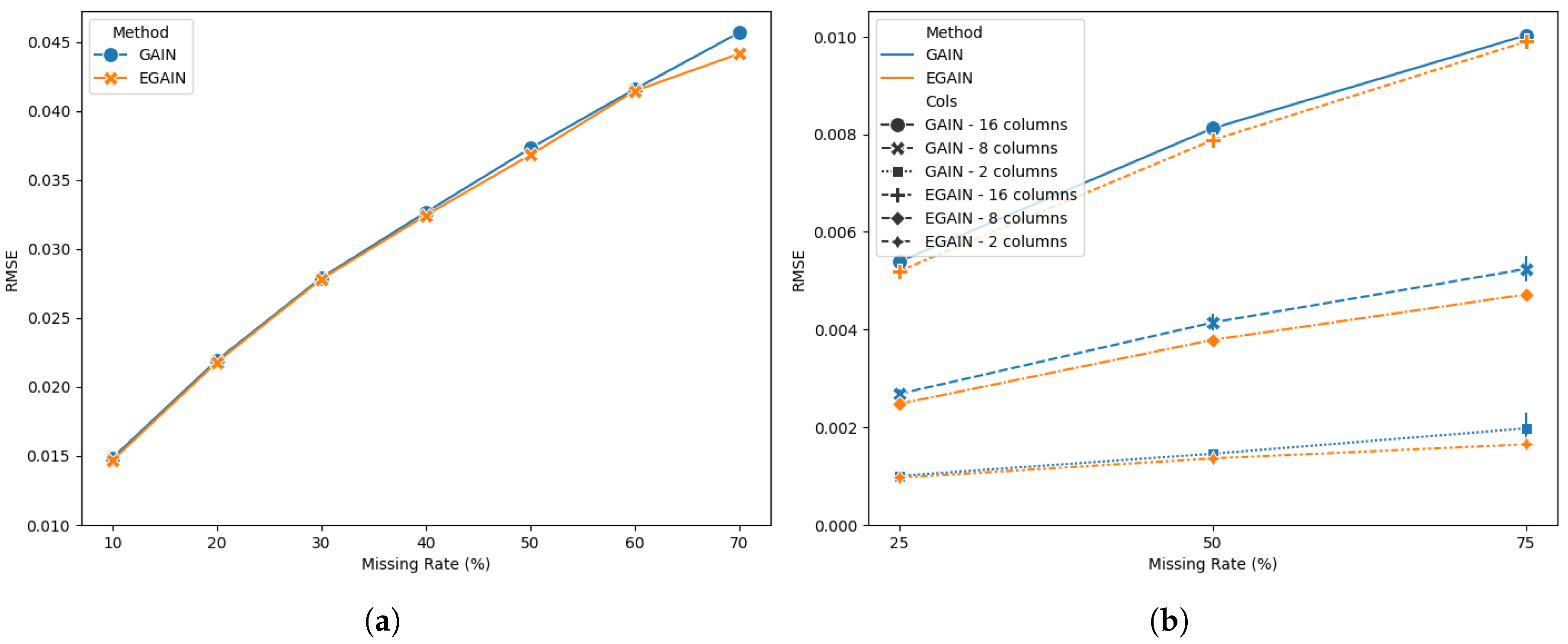
Figure 4.
Performance comparison of GAIN vs EGAIN for credit dataset: (a) MCAR from the 14 numerical columns. (b) MCAR from randomly selected columns among 14 numerical features.
Figure 4.
Performance comparison of GAIN vs EGAIN for credit dataset: (a) MCAR from the 14 numerical columns. (b) MCAR from randomly selected columns among 14 numerical features.
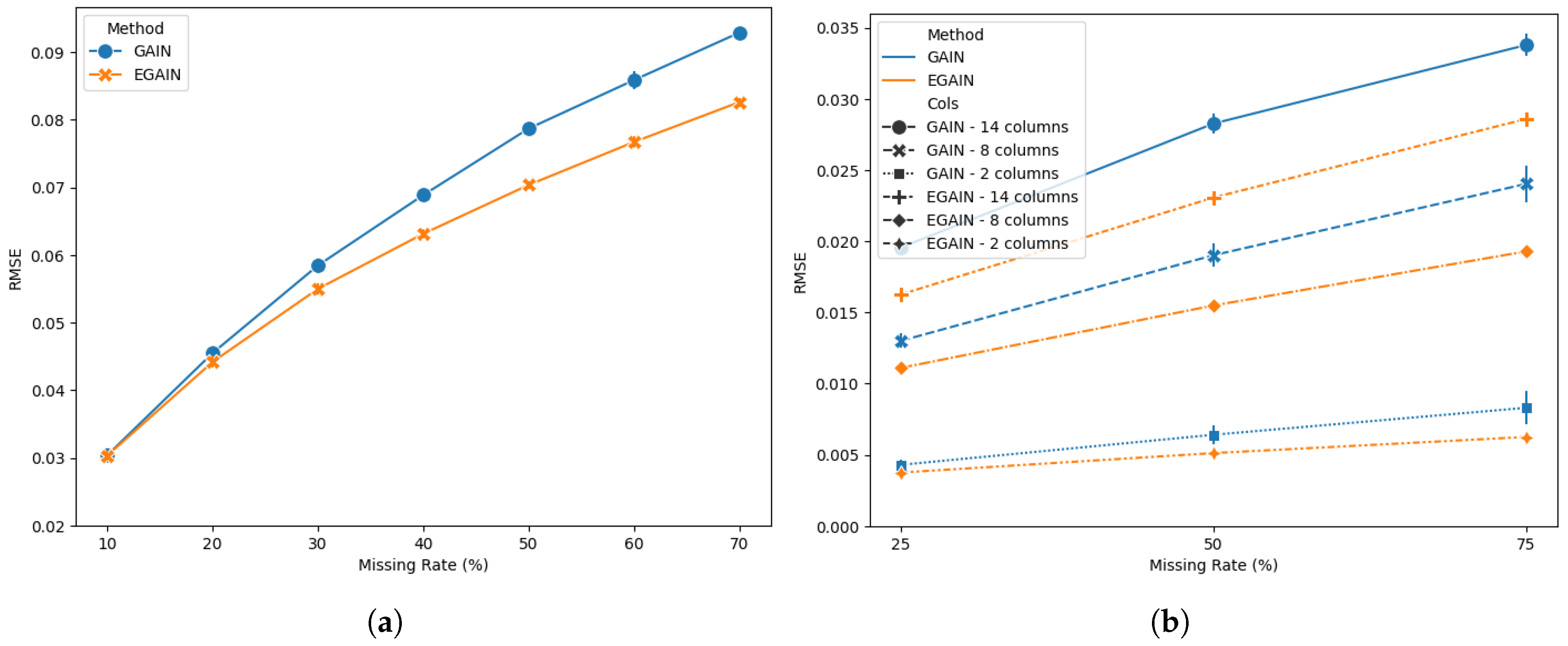

Table 1.
Benchmark datasets (small, medium, large).
| Dataset | Cases | Features | Description |
|---|---|---|---|
| breast | 569 | 31 | 30 numerical, 1 binary categorical |
| spam | 4,601 | 58 | 57 numerical, 1 binary categorical |
| credit | 30,000 | 24 | 14 numerical, 10 categorical |
Table 2.
Overall imputation performance across experiments in terms of RMSE (Average ± Std).
| Method | GAIN | EGAIN |
|---|---|---|
| breast cancer | 0.0385 ± 0.0331 | 0.0373 ± 0.0314 |
| spam | 0.0200 ± 0.0157 | 0.0161 ± 0.0152 |
| credit | 0.0413 ± 0.0284 | 0.0345 ± 0.0263 |
Disclaimer/Publisher’s Note: The statements, opinions and data contained in all publications are solely those of the individual author(s) and contributor(s) and not of MDPI and/or the editor(s). MDPI and/or the editor(s) disclaim responsibility for any injury to people or property resulting from any ideas, methods, instructions or products referred to in the content. |
© 2025 by the authors. Licensee MDPI, Basel, Switzerland. This article is an open access article distributed under the terms and conditions of the Creative Commons Attribution (CC BY) license (http://creativecommons.org/licenses/by/4.0/).
Copyright: This open access article is published under a Creative Commons CC BY 4.0 license, which permit the free download, distribution, and reuse, provided that the author and preprint are cited in any reuse.


