
Submitted:
17 April 2025
Posted:
17 April 2025
You are already at the latest version
Abstract
This paper establishes a foundational framework for the application of Generative AI in financial risk management by providing a comprehensive overview and review of essential quantitative techniques. We illustrate the quantitative aspect of these models in equity, fixed income, and mortgage-backed securities markets, emphasizing their proposed Gen AI enhancement in enhancing risk management practices. Furthermore, this paper examines the transformative potential of Generative AI, specifically Generative Adversarial Networks (GANs) and Variational Autoencoders (VAEs), in reshaping risk modeling and stress testing. We bridge classical quantitative techniques—including Monte Carlo methods, Value-at-Risk, and stochastic processes—with modern generative models like GANs and VAEs. The study first reviews foundational models for market, credit, and liquidity risk, demonstrating their application across fixed income and mortgage-backed securities markets. We then propose novel AI-enhanced methodologies for: (1) liquidity risk quantification through augmented Monte Carlo simulations, (2) dynamic credit risk modeling using agentic frameworks, and (3) stress testing with synthetic scenario generation. A key contribution is the development of hybrid architectures that combine traditional risk metrics with data-driven generative AI, implemented through practical Python workflows. The paper concludes with empirical results showing improved accuracy in Expected Liquidity Shortfall (ELS) estimation and Value-at-Risk calculations, providing a pathway for next-generation risk management systems. By laying this quantitative foundation, we aim to facilitate the adoption of advanced Gen AI techniques, offering a forward-looking perspective on the future of quant-data-driven financial risk management.
Keywords:
Market Risk
; Credit Risk
; Liquidity Risk
; Monte Carlo Simulation
; Value-at-Risk
; Extreme Value Theory
; Mortgage-Backed Securities
; Blockchain
; Generative AI
; Stochastic Processes
; Risk Modeling
1. Introduction
Financial institutions operate within an intricate and dynamic environment, confronting a spectrum of risks—market, credit, and liquidity—that can significantly challenge their operational resilience relying highly on data and quant modeling. Traditional risk management methodologies, while foundational, are increasingly being augmented to address the complexities of modern financial markets. This paper extends beyond conventional and conservative approaches by proposing integration of mathematical models with Generative AI.
Generative AI models hold significant promise for revolutionizing stress testing and scenario analysis. By generating realistic market simulations, these models enable institutions to explore a wider range of potential outcomes, thereby enhancing predictive accuracy and robustness. Furthermore, AI-driven risk models offer the capability to adapt to rapidly changing market conditions, providing a dynamic and responsive risk management framework.
To effectively leverage the power of Generative AI in financial risk management, a solid understanding of the underlying mathematical models governing liquidity and market risks is essential. This paper will delve into these foundational quantitative models, exploring stochastic processes, Monte Carlo simulations, and Extreme Value Theory, which form the bedrock of quantitative risk assessment. We will then transition to examining the practical applications of these models in various financial markets, including equity, fixed income, and mortgage-backed securities, demonstrating their relevance in real-world scenarios. Finally, we will explore how Generative AI can be integrated with these established methodologies to create a more sophisticated and adaptive risk management paradigm.
2. Literature Review
The field of financial risk management has witnessed significant advancements in quantitative techniques, driven by the increasing complexity of financial markets and the need for more robust risk assessment methodologies. This paper draws upon a mix of old (liquidity risk) and new (gen ai) body of literature spanning various aspects of market, credit, and liquidity risk, as well as the emerging applications of Generative AI.
2.1. Foundational Risk Management Concepts: Classical Overview
Monte Carlo Methods:[1] provides a comprehensive overview of Monte Carlo methods in financial engineering, highlighting their versatility in risk management, derivative pricing, and portfolio optimization. Value-at-Risk (VaR): [2] discusses the evolution and widespread adoption of Value-at-Risk (VaR) as a cornerstone metric in market risk management, emphasizing its role in quantifying potential losses. Credit Risk Modeling: [3] lays the groundwork for structural credit risk models, which have become indispensable tools for assessing default probabilities and managing credit exposures.
2.2. Liquidity Risk Dynamics
Market Liquidity and Financial Stability: [4] delves into the intricate dynamics of market liquidity, particularly its impact on financial stability during crises, underscoring the importance of liquidity risk management. Bid-Ask Spreads and Asset Pricing: [5] examines the influence of bid-ask spreads on asset pricing, shedding light on the crucial role of liquidity considerations in fixed income markets. Credit Risk with Liquidity Considerations: [6] develops a framework for modeling credit risk that incorporates liquidity risk, recognizing the interconnectedness of these risk categories.
2.3. Mortgage-Backed Securities (MBS) Risk
Prepayment Risk in MBS: [7] analyzes the prepayment risk inherent in mortgage-backed securities (MBS), providing insights essential for accurate valuation and risk assessment. Option-Theoretic Valuation of Mortgages: [8] proposes an option-theoretic approach to valuing residential mortgages, recognizing the embedded optionality in these contracts.
2.4. Generative AI in Finance
Generative Adversarial Networks (GANs): [9] introduces Generative Adversarial Networks (GANs), a powerful class of generative models with potential applications in finance, including generating realistic market scenarios for stress testing and risk modeling. Variational Autoencoders (VAEs): [10] presents Variational Autoencoders (VAEs), another type of generative model that can be used to learn latent representations of financial data, enabling the generation of synthetic data and enhancing risk analysis.
This literature review provides a foundation for the quantitative techniques and Generative AI applications explored in this paper, demonstrating the ongoing evolution of financial risk management methodologies.
3. Fixed Income Markets and Risk Management
Fixed income securities, including government and corporate bonds, play a crucial role in financial markets. Managing risk in fixed income involves interest rate risk, credit risk, and liquidity risk.
3.1. Interest Rate Risk
Interest rate risk is typically measured using duration and convexity:
where D is the duration, P is the bond price, and y is the yield.
Convexity improves the accuracy of price sensitivity estimation:
3.2. Credit Risk
The probability of default (PD) is estimated using structural models such as Merton’s model:
where is the firm value at time T, B is the debt threshold, and is the standard normal cumulative distribution function.
3.3. Liquidity Risk in Fixed Income
Liquidity risk in fixed income is assessed using bid-ask spreads and market depth:
where L is the liquidity measure, and and represent the respective prices.
Monte Carlo simulations are employed to stress-test bond portfolios under various yield curve scenarios.
4. Credit Risk in Mortgage-Backed Securities
Mortgage-Backed Securities (MBS) introduce unique credit risks due to prepayment risk and default risk.
4.1. Credit Risk in Mortgage-Backed Securities
MBS risks include prepayment:
default:
and loss given default:
4.2. Prepayment Risk
Prepayment risk is modeled using the Conditional Prepayment Rate (CPR):
where is the Single Monthly Mortality rate.
4.3. Default Risk
The probability of default in MBS can be modeled using a logistic regression approach:
where is the credit score, is the loan-to-value ratio, and is the debt-to-income ratio.
4.4. Loss Given Default (LGD)
LGD is estimated using historical recovery rates:
where is the recovered amount from foreclosure sales.
Monte Carlo simulations are used to simulate default probabilities and cash flow losses under stressed economic conditions.
5. Liquidity Risk Management
Effective liquidity risk management necessitates a blend of strategic planning and quantitative analysis. In this section, we examine practical strategies such as dynamic hedging and collateralized funding, which institutions employ to manage liquidity exposures. Furthermore, we propose Gen AI enhancement of the the mathematical models used to quantify liquidity risk, including the Liquidity Coverage Ratio (LCR), stochastic processes like the Vasicek model, and Monte Carlo simulations for estimating Expected Liquidity Shortfall (ELS).
Figure 1 Figure 2, Figure 3, Figure 4, Figure 5, Figure 6, etc demonstrates classical and the proposed architectures.
5.1. Managing Market and Liquidity Risk Exposures
Strategies include dynamic hedging:
collateralized funding:
and liquidity stress testing:
Liquidity risk is the inability to meet short-term financial obligations. It is measured using the Liquidity Coverage Ratio (LCR):
where represents High-Quality Liquid Assets, and is the Total Net Cash Outflows over 30 days.
A stochastic approach to liquidity spread can be modeled using the Vasicek model:
where is the liquidity spread, is the mean reversion rate, is the long-run mean, and is a Wiener process.
Monte Carlo simulations estimate Expected Liquidity Shortfall (ELS):
6. Margining in Market Risk Management
Margining controls counterparty risk. Initial Margin (IM) is determined using Value-at-Risk (VaR):
where is the expected return, is the standard deviation, and is the Z-score at confidence level .
Expected Shortfall (Conditional VaR) provides a better measure of tail risk:
This integral represents the average loss beyond the VaR threshold, capturing the severity of losses in extreme scenarios.
6.1. Stress Testing
Stress testing evaluates market risk under extreme conditions. A linear factor model for portfolio return is:
where are macroeconomic factors, and are sensitivities. This model allows for the assessment of portfolio sensitivity to various macroeconomic shocks.
Extreme Value Theory (EVT) models tail risk using the Generalized Pareto Distribution (GPD):
where is the tail index, u is the threshold, and is the scale parameter. EVT focuses on modeling the tails of distributions, which are crucial for capturing extreme events.
Monte Carlo simulations apply macroeconomic shocks to compute worst-case losses, providing a more comprehensive view of potential losses under stress.
6.2. Equity Financial Markets and Products
Equity financial markets involve the trading of stocks and related instruments, many of which are cleared and settled at central clearing houses such as the National Securities Clearing Corporation (NSCC) and the Depository Trust Company (DTC).
Clearing houses mitigate counterparty risk using a multi-tiered risk framework. The clearing fund requirement is calculated as:
where is the clearing fund, is the Value-at-Risk for participant i, and is the initial margin requirement.
Settlement risk is managed through a rolling settlement cycle and netting mechanisms. The netting efficiency ratio is given by:
where represents the total gross trade values and represents net settlement amounts post-clearing.
Monte Carlo simulations assess the impact of market stress on clearing fund adequacy by simulating extreme price movements and evaluating liquidity shortfalls.
6.3. Managing Market and Liquidity Risk Exposures
Historically, financial institutions have employed various strategies to manage market and liquidity risks.
6.3.1. Dynamic Hedging
A risk-mitigating strategy that adjusts positions in response to market movements. The delta-neutral strategy ensures that a portfolio’s sensitivity to small price changes remains minimal:
where is the portfolio delta, and represent the delta and stock price of individual assets.
6.3.2. Collateralized Funding
Repo agreements and secured funding mechanisms ensure liquidity adequacy. The haircut applied to collateralized borrowing is computed as:
where is the market value of collateral, and is the collateral-adjusted price.
6.3.3. Liquidity Stress Testing
By simulating liquidity outflows under extreme conditions, firms estimate the survival horizon:
where is the survival horizon, and represents projected total outflows over time.
These strategies, combined with regulatory liquidity requirements, help financial institutions maintain stability under adverse market conditions.
Liquidity risk, the inability to meet short-term financial obligations, is critical. The Liquidity Coverage Ratio (LCR) is defined as:
where represents High-Quality Liquid Assets, and is the Total Net Cash Outflows over 30 days.
We can model liquidity spread using the Vasicek model, a mean-reverting stochastic process:
where is the liquidity spread, is the mean reversion rate, is the long-run mean, and is a Wiener process. This model captures the tendency of liquidity spreads to revert to their long-term average, providing a dynamic view of liquidity conditions.
Monte Carlo simulations estimate Expected Liquidity Shortfall (ELS):
This involves simulating various scenarios of cash flows and asset values to estimate the probability and magnitude of liquidity shortfalls.
| Algorithm 1 Monte Carlo Simulation for ELS |
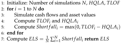 |
7. Liquidity Risk and Market Risk Mathematical Models
In this section, we explore the key mathematical models used in the assessment and management of both liquidity risk and market risk, which are essential for financial institutions and their risk management frameworks.
7.1. Liquidity Risk Models
Liquidity risk refers to the possibility that an entity may be unable to meet its short-term financial obligations due to an imbalance between its liquid assets and liabilities. Below are some common models used to quantify liquidity risk:
7.1.1. Cash Flow Models
Cash flow models analyze the inflows and outflows of cash to identify potential liquidity shortfalls. The general equation for cash flow modeling is given by:
where represents the cash flow at time t, is the previous period’s cash balance, and and are the expected inflows and outflows at time t.
7.1.2. Liquidity Coverage Ratio (LCR)
The Liquidity Coverage Ratio (LCR) is a regulatory requirement for banks to maintain an adequate level of high-quality liquid assets to cover short-term obligations. The formula for LCR is:
7.1.3. Stochastic Liquidity Risk Models
Liquidity risk is sometimes modeled as a stochastic process. The liquidity level at time t, denoted as , can be described by the stochastic differential equation (SDE):
where is the liquidity at time t, represents the drift (average rate of change), is the volatility, and is the Wiener process representing random shocks.
7.1.4. Transaction Cost Models
Transaction cost models help assess the impact of liquidity on trade execution. A simple form of the transaction cost model is:
where market impact models, such as Kyle’s and Hasbrouck’s models, capture the relationship between the size of a trade and its impact on the market price.
7.2. Market Risk Models
Market risk refers to the risk of losses in positions due to movements in market prices, including changes in interest rates, asset prices, and commodity prices. Below are some common models used to assess market risk:
7.2.1. Value-at-Risk (VaR)
Value-at-Risk (VaR) is a widely used method for measuring market risk, which estimates the maximum loss over a specified time horizon at a given confidence level. The formula for VaR is:
where represents the confidence level (e.g., 95% or 99%), and the quantile is determined based on the distribution of portfolio returns.
7.2.2. Conditional Value-at-Risk (CVaR)
Conditional Value-at-Risk (CVaR), also known as Expected Shortfall, measures the expected loss given that the loss exceeds the VaR threshold. The formula for CVaR is:
where X represents the portfolio loss.
7.2.3. GARCH Models
The Generalized Autoregressive Conditional Heteroskedasticity (GARCH) model is widely used for estimating the volatility of asset returns. The GARCH(1,1) model is defined as:
where is the return at time t, is the innovation or shock, represents the conditional variance, and is a white noise process.
7.2.4. Stochastic Volatility Models
Stochastic volatility models capture the evolution of volatility over time. The Heston model, a popular stochastic volatility model, is expressed as:
where represents the asset price, is the volatility process, and , are Wiener processes.
7.2.5. Monte Carlo Simulation
Monte Carlo simulations are used to estimate the potential losses or profits in financial portfolios by generating multiple scenarios for asset prices and other risk factors. The general form of Monte Carlo simulations is:
where N is the number of simulations, is the payoff in each scenario, and is the probability of each scenario occurring.
7.2.6. Copula Models
Copula models are used to model the joint distribution of multiple risk factors. A commonly used copula is the Gaussian copula, which connects the marginal distributions of asset returns:
where C is the copula function, and are the marginal distributions.
7.3. Monte Carlo Simulation for Liquidity Risk
Monte Carlo simulation is a powerful technique used to model and quantify liquidity risk by generating multiple scenarios for cash flows, liquidity shortfalls, and funding needs under various conditions. By simulating different scenarios based on stochastic processes, Monte Carlo methods help in assessing the likelihood of liquidity shortages and determining the adequacy of liquidity buffers under stressed conditions.
7.3.1. Stochastic Processes in Liquidity Risk Modeling
In liquidity risk modeling, stochastic processes are used to describe the evolution of liquidity levels and related risk factors over time. These processes capture the inherent uncertainty in cash flows, market conditions, and funding requirements. Below are some common stochastic processes used in Monte Carlo simulations for liquidity risk:
Geometric Brownian Motion (GBM) for Cash Flow Modeling
For modeling the liquidity levels over time, the Geometric Brownian Motion (GBM) is often used to represent the continuous evolution of liquidity in a firm or financial institution. The equation for GBM applied to liquidity is:
where represents the liquidity level at time t, is the drift (representing expected liquidity growth or reduction), is the volatility (representing uncertainty in liquidity fluctuations), and is the Wiener process (representing random shocks in the market). This model can simulate multiple future paths of liquidity, accounting for both expected trends and random fluctuations.
Ornstein-Uhlenbeck Process for Mean Reversion in Liquidity
Liquidity levels in certain financial institutions or markets may exhibit mean-reverting behavior, where liquidity tends to revert to a long-term average over time. The **Ornstein-Uhlenbeck (OU) process** is a common stochastic process used to model such mean-reverting behavior. The equation for the OU process in liquidity modeling is:
where is the liquidity level at time t, is the rate of mean reversion (how quickly liquidity returns to the long-term mean ), and is the volatility. This process is useful when modeling scenarios where liquidity fluctuations are expected to stabilize around a certain value (e.g., target liquidity levels maintained by a bank).
Jump-Diffusion Model for Liquidity Shocks
Financial markets and liquidity positions can be affected by sudden, extreme events such as financial crises, liquidity squeezes, or regulatory changes. The **Jump-Diffusion model** is used to model these types of liquidity shocks. The equation for the Jump-Diffusion model in liquidity modeling is:
where represents the jump size (the magnitude of liquidity shocks), and is a Poisson process that represents the arrival of jumps at random times. This model is suitable for simulating scenarios where liquidity shortfalls may occur abruptly due to large market shocks, such as credit downgrades, unexpected market closures, or regulatory interventions.
Stochastic Volatility Models for Liquidity Risk
In some cases, liquidity risk is closely related to the volatility of market conditions, such as fluctuations in funding costs or asset prices. The **Heston model**, a stochastic volatility model, can be applied to liquidity risk when volatility in funding costs or liquidity premiums is non-constant. The Heston model is given by two SDEs:
where represents the liquidity level, is the volatility of liquidity (funding costs or liquidity premium), and , are Wiener processes representing random shocks. This model allows for the simulation of liquidity levels in environments with fluctuating funding costs and market volatility.
7.3.2. Implementation of Monte Carlo Simulation for Liquidity Risk
The implementation of Monte Carlo simulations for liquidity risk typically involves the following steps:
- Modeling Liquidity Dynamics: Select an appropriate stochastic process to model the evolution of liquidity (e.g., GBM, Ornstein-Uhlenbeck, Jump-Diffusion).
- Simulating Liquidity Paths: Using the chosen stochastic process, simulate multiple paths for liquidity levels over a defined time horizon, factoring in different levels of funding needs and market conditions.
- Estimating Liquidity Shortfalls: For each simulated liquidity path, calculate potential liquidity shortfalls by comparing liquidity levels to projected funding needs or cash flow obligations at various points in time.
- Stress Testing: Apply extreme market conditions (e.g., sudden shocks or increased volatility) to assess the robustness of liquidity buffers and the likelihood of liquidity crises.
- Aggregating Results: Analyze the distribution of liquidity shortfalls, and estimate the probability of liquidity gaps under different scenarios, providing a risk measure for liquidity risk management.
Monte Carlo simulations for liquidity risk provide critical insights into the stability of an institution’s liquidity position under a variety of scenarios. By simulating many potential future outcomes, risk managers can better understand the probability of liquidity shortages and prepare strategies to mitigate such risks.
7.3.3. Conclusion for MC for Liquidity
Monte Carlo simulation, when combined with appropriate stochastic processes, is a valuable tool for modeling liquidity risk. It allows financial institutions to assess the potential for liquidity shortfalls, the effectiveness of liquidity buffers, and the impact of extreme market events on liquidity positions. This approach is essential for stress testing and effective liquidity risk management.
7.4. GANs and VAEs in Liquidity Risk Monte Carlo Simulations for VaR Calculation
Generative models, such as Generative Adversarial Networks (GANs) and Variational Autoencoders (VAEs), have shown great potential in enhancing Monte Carlo simulations for liquidity risk modeling, especially when calculating Value-at-Risk (VaR). These models can be used to generate realistic synthetic data for liquidity scenarios, capturing complex patterns and dependencies that traditional stochastic processes may miss. By incorporating these generative models, financial institutions can more accurately simulate liquidity risk and assess the potential for large, adverse liquidity events.
7.4.1. Value-at-Risk (VaR) and Liquidity Risk
Value-at-Risk (VaR) is a widely used risk metric to estimate the potential loss in the value of a portfolio over a specified time horizon, given a certain confidence level. In the context of liquidity risk, VaR is used to assess the potential liquidity shortfall that could occur under stressed market conditions. Monte Carlo simulations are typically employed to simulate multiple scenarios of asset prices, funding needs, and cash flows over time, but traditional methods can sometimes be limited in their ability to fully capture the complexity of liquidity dynamics.
7.4.2. Using GANs for Liquidity Risk Simulation
Generative Adversarial Networks (GANs) consist of two neural networks—the generator and the discriminator—that work in tandem to create realistic data by learning the distribution of the input data. In the context of liquidity risk, GANs can be used to generate synthetic liquidity paths or asset price scenarios that resemble real-world data while capturing complex non-linear relationships, correlations, and tail risks.
The process involves training the GAN on historical liquidity data or financial market data to learn the underlying distribution. Once trained, the generator can create realistic future liquidity scenarios under different conditions, which can then be incorporated into Monte Carlo simulations for VaR calculations. These scenarios can capture extreme liquidity shortfalls or unexpected market disruptions, which are often difficult to model using traditional stochastic processes like Geometric Brownian Motion (GBM).
The use of GANs in liquidity risk modeling offers several advantages:
- Capturing Complex Dependencies: GANs can model complex, non-linear relationships between liquidity factors, such as correlations between asset prices, funding costs, and liquidity requirements.
- Generating Extreme Scenarios: GANs can generate rare but impactful liquidity events (e.g., market crashes or sudden funding squeezes) that are essential for accurate VaR estimation, particularly in tail risk analysis.
- Data Augmentation: GANs can generate large quantities of synthetic data to enhance the Monte Carlo simulation process, improving the accuracy and robustness of the VaR calculation.
7.4.3. Using VAEs for Liquidity Risk Simulation
Variational Autoencoders (VAEs) are another class of generative models that can be particularly useful for liquidity risk modeling. VAEs are designed to learn an efficient representation of input data by encoding it into a latent space and then decoding it back into data. The latent space captures the essential features of the data, allowing for the generation of new, similar data points by sampling from this latent space.
In the context of liquidity risk, VAEs can be used to learn the underlying distribution of liquidity levels, funding requirements, or market conditions over time. Once trained, VAEs can generate synthetic liquidity paths that are consistent with observed data but may explore previously unseen scenarios that are still realistic, helping to account for rare or extreme liquidity events.
The use of VAEs in liquidity risk modeling offers several benefits:
- Efficient Data Representation: VAEs can learn a compressed representation of liquidity risk factors, which can then be used to generate new, diverse liquidity scenarios, improving the efficiency and speed of Monte Carlo simulations.
- Exploring Unseen Scenarios: By sampling from the learned latent space, VAEs can generate liquidity scenarios that are not directly observed in historical data but still reflect the underlying structure of the data. This is particularly useful for stress testing under hypothetical scenarios.
- Reducing Overfitting: Since VAEs generate data based on learned distributions, they help reduce overfitting to historical data, ensuring that Monte Carlo simulations account for a wider range of potential future outcomes.
7.4.4. Integration of GANs and VAEs into Monte Carlo Simulations for VaR Calculation
By combining GANs and VAEs with Monte Carlo simulations, financial institutions can enhance their ability to model liquidity risk and accurately calculate Value-at-Risk (VaR). The process can be outlined as follows:
- Data Preparation: Historical liquidity and financial data are collected to train the GAN or VAE models. This data could include cash flow information, funding requirements, asset prices, and other relevant risk factors.
- Training the Generative Model: The GAN or VAE model is trained on this historical data to learn the distribution and correlations between liquidity risk factors. The generator in the GAN or the decoder in the VAE learns to produce realistic synthetic data based on this training.
- Scenario Generation: Once trained, the GAN or VAE can generate synthetic liquidity paths or asset price scenarios that reflect the learned distribution, including rare or extreme scenarios that are important for accurate VaR estimation.
- Monte Carlo Simulation: These generated scenarios are then fed into a Monte Carlo simulation framework, where they are used to simulate the potential future liquidity levels, funding needs, and cash flows under different market conditions.
- VaR Calculation: After running the Monte Carlo simulation with the synthetic scenarios, the Value-at-Risk (VaR) is calculated by assessing the distribution of potential liquidity shortfalls or losses over the specified time horizon and confidence level.
By integrating GANs and VAEs into the Monte Carlo simulation process, financial institutions can gain a deeper understanding of liquidity risk and obtain more accurate estimates of VaR. These generative models enhance the ability to model complex, non-linear relationships, generate extreme scenarios, and explore unseen risks, leading to better risk management and more robust liquidity buffers.
7.4.5. Conclusion of GANs and VAEs
The use of Generative Adversarial Networks (GANs) and Variational Autoencoders (VAEs) in Monte Carlo simulations for liquidity risk modeling represents a significant advancement in the field of risk management. By generating realistic, diverse liquidity scenarios and capturing complex dependencies, these generative models provide enhanced accuracy in Value-at-Risk (VaR) calculations. This approach allows financial institutions to better assess liquidity risks, stress-test their portfolios under extreme conditions, and make more informed decisions regarding liquidity buffers and funding strategies.
7.5. Market Impact Models and Mathematical Models in Liquidity Risk
Market impact models are essential in understanding how large trades, such as those required for liquidity management or hedging strategies, affect asset prices and market liquidity. These models quantify the relationship between trade size and price movement, helping financial institutions evaluate the potential cost of executing large trades under varying market conditions. Properly understanding market impact is crucial for managing liquidity risk, as large trades can cause slippage, increase volatility, or even trigger adverse market reactions.
7.5.1. Types of Market Impact
Market impact can be broadly categorized into two main types:
- Temporary Impact: This refers to the short-term price movement caused by a trade. Once the trade is executed, the price often reverts back to its original level.
- Permanent Impact: This is the long-term price shift caused by a trade, which does not fully revert after the transaction is completed. It is typically the result of significant market information being revealed by the trade (e.g., large buy or sell orders indicating a shift in market sentiment).
Market impact models aim to capture both the temporary and permanent effects of a trade on market prices, as these impacts are key components of liquidity risk and transaction cost estimation.
7.5.2. Mathematical Models for Market Impact
Several mathematical models are used to quantify market impact, often focusing on the relationship between trade size, market depth, and asset price movements. Below are some of the most commonly used models:
The Almgren-Chriss Model
The Almgren-Chriss model is one of the foundational models in market impact theory. It assumes that the price impact is a function of both the size of the trade and the time over which the trade is executed. The model divides the total transaction cost into two components: the temporary market impact and the permanent market impact. The equations for the Almgren-Chriss model are as follows:
The temporary impact is typically modeled as a quadratic function of the order size, Q, and the permanent impact as a linear function of the order size. The temporary market impact can be written as:
where is a constant that depends on market liquidity and the volatility of the asset.
The permanent market impact is often modeled as:
where represents the permanent price impact per unit of trade size. The parameters and are typically estimated using historical market data, such as trade sizes and price movements.
The Kyle Model
The Kyle model is another influential framework for understanding market impact. It assumes that the market consists of a single informed trader, a liquidity provider (market maker), and other noise traders. The informed trader, knowing the true value of an asset, adjusts their trading strategy to influence the market price. The market maker sets the price based on the trades, attempting to offset the risk from informed traders. The equilibrium price in the Kyle model is given by:
where is the observed price at time t, is the true asset value, is the trade size at time t, and represents noise in the market. The parameter captures the sensitivity of the price to the trade size, and the model predicts that large trades cause larger price movements, with the market maker adjusting the price to account for the information contained in the trade.
The Kyle model has been extended to incorporate multiple market makers and various types of traders, but the central insight remains that price impact increases with the size of the trade.
The Liquidity Ripple Model
The Liquidity Ripple model focuses on the persistence of price changes caused by large trades. This model incorporates the idea that market impact can have a ripple effect, where the initial price movement due to a large trade can influence subsequent trades and prices. The model assumes that liquidity shockwaves propagate through the market, affecting asset prices for a certain period after the transaction is executed. The mathematical formulation of the ripple effect is represented by:
where is the price at time t, Q is the trade size, is the time horizon over which the impact is measured, and is a constant that measures the ripple effect. The model suggests that large trades induce not only an immediate price impact but also a persistent influence on market prices over time, which can be critical when calculating liquidity risk and stress testing.
The Epps Model
The Epps model describes the relationship between asset price volatility and the market’s response to trading activity. This model assumes that asset price movements are influenced by both fundamental factors and the trading activity of large institutional players. The model suggests that trading activity causes volatility clustering, where large trades lead to periods of increased price volatility. The model is often expressed as:
where is the asset price volatility at time t, is the trade size, and and are constants that reflect the baseline volatility and the impact of trading on volatility, respectively. This model is useful for understanding how trading volume and market depth contribute to overall price volatility and liquidity risk.
7.5.3. Market Impact in Liquidity Risk Management
In liquidity risk management, understanding and quantifying market impact is essential for estimating the costs of executing large trades and assessing the potential liquidity shortfalls under various scenarios. By incorporating market impact models into Monte Carlo simulations, financial institutions can better predict the effects of large trades on asset prices and liquidity, and adjust their liquidity buffers accordingly.
For instance, in a Value-at-Risk (VaR) calculation, market impact models can be used to simulate the effect of trading large positions in a portfolio on the price of assets. By including transaction costs and the impact on liquidity in the VaR calculation, institutions can more accurately estimate the potential loss under stressed market conditions, incorporating both market volatility and liquidity constraints.
7.5.4. Conclusion on Liq Models and Maths
Market impact models are critical tools in understanding how liquidity risk manifests during large trades and market disruptions. By using mathematical models such as the Almgren-Chriss, Kyle, Liquidity Ripple, and Epps models, financial institutions can quantify the effects of trade size and market depth on asset prices. These models help to predict transaction costs, price slippage, and liquidity shortfalls, providing valuable insights for liquidity risk management and enhancing the accuracy of simulations used in VaR calculations. With accurate market impact models, financial institutions can better manage liquidity, minimize costs, and improve the robustness of their risk management strategies.
8. Future Work and Integration with Generative AI
As financial markets continue to evolve, the application of advanced artificial intelligence (AI) techniques in financial risk modeling becomes increasingly critical. The integration of generative AI models, such as Variational Autoencoders (VAEs) and Generative Adversarial Networks (GANs), into traditional risk frameworks like the Vasicek model, will drive future advancements in more accurate and dynamic financial risk prediction and management. Future research will focus on further enhancing these models by incorporating agentic generative AI techniques, enabling more adaptive, data-driven risk management strategies.
One promising area for development is the refinement of the Vasicek framework using agentic generative AI. By leveraging the potential of generative models to simulate complex, high-dimensional financial data, we can significantly improve the modeling of stochastic processes that underlie asset prices and financial instruments. The use of generative AI to simulate diverse market scenarios will also aid in the creation of robust stress-testing frameworks, providing a more comprehensive assessment of potential financial disruptions and systemic risks [11].
Furthermore, advancing innovation in financial stability through AI agent frameworks offers significant potential. These frameworks can automate the detection of market anomalies, thereby contributing to more effective financial regulatory systems. The ability to simulate various market conditions and agent behaviors will enable regulators to predict and mitigate potential crises before they fully materialize [12]. Future work will involve creating more sophisticated agent-based models that incorporate feedback loops between financial institutions, market participants, and regulatory authorities, fostering a more resilient financial ecosystem.
The role of VAEs and GANs in improving structured finance risk models is another key area of focus. By utilizing generative models, we can enhance the Leland-Toft and Box-Cox models for pricing and managing complex financial products. The future of risk management will undoubtedly see increased adoption of AI-driven methodologies for better forecasting of liquidity needs, market movements, and systemic risk [13].
In addition, the development of AI tools for enhancing the robustness of the US financial and regulatory systems is expected to play a central role in future research. By leveraging generative AI, we can design models that adapt to regulatory changes and evolving market conditions, ensuring a more dynamic and responsive financial environment [14].
The continued exploration of generative AI models for financial risk management will also encompass the review and comparison of existing models, identifying gaps and proposing new methodologies for better financial predictions and risk assessments. As the capabilities of AI evolve, integrating large language models (LLMs) and other advanced AI tools into financial risk management systems will allow for the processing of complex data sets and the automation of decision-making processes, enhancing both efficiency and accuracy [15].
Finally, understanding the synergy between generative AI and big data will be critical for the future of financial risk management. The ability to process vast amounts of financial data in real-time, combined with generative AI’s capacity to model and simulate complex risk scenarios, will enable more informed decision-making in market risk management [16].
Overall, future work in this area will aim to improve financial market integrity through the continued development of AI models, such as prompt engineering, and the refinement of risk management frameworks to ensure that they are adaptable to the fast-changing financial landscape [17].
9. Proposed Algorithm
The proposed framework integrates traditional risk models with generative AI components through the following algorithmic workflow:
| Algorithm 2 Generative AI for Risk Management |
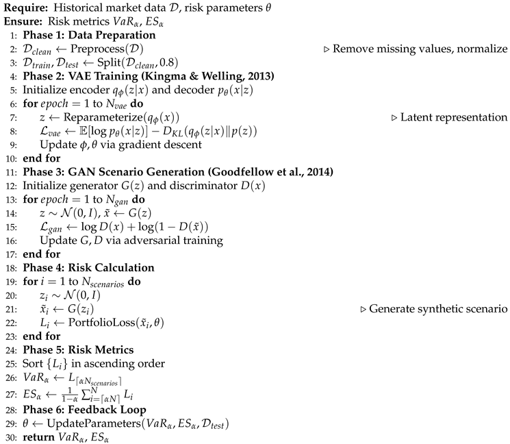 |
The algorithm combines several key components from the literature:
- VAE Training (Line 4-8): Following [10], we learn compressed latent representations of market data
- GAN Scenario Generation (Line 10-14): Adversarial training as in [9] produces realistic stress scenarios
- Risk Calculation (Line 16-20): Monte Carlo simulation using synthetic scenarios
- Metrics Computation (Line 22-24): Value-at-Risk and Expected Shortfall calculation per [2]
- Feedback Mechanism: Continuous model improvement via parameter updates
10. Proposed Python Implementation
This section provides sample Python code to illustrate the implementation of key quantitative techniques discussed in the paper, including Monte Carlo simulations, Generative Adversarial Networks (GANs), and Variational Autoencoders (VAEs). The code snippets are designed to be modular and can be adapted for real-world financial risk management applications.
10.1. Monte Carlo Simulation for Liquidity Risk
The following Python code demonstrates a Monte Carlo simulation for estimating Expected Liquidity Shortfall (ELS) using stochastic processes.
| Listing 1: Monte Carlo Simulation for Liquidity Risk |
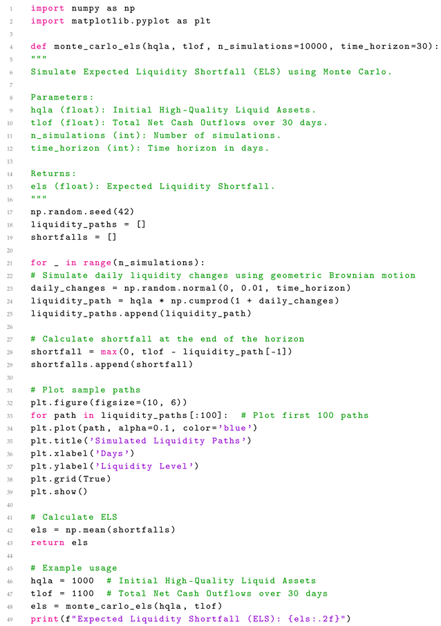 |
10.2. Generative Adversarial Networks (GANs) for Scenario Generation
The following code snippet demonstrates a simplified GAN implementation for generating synthetic financial scenarios.
| Listing 2: GAN for Financial Scenario Generation |
 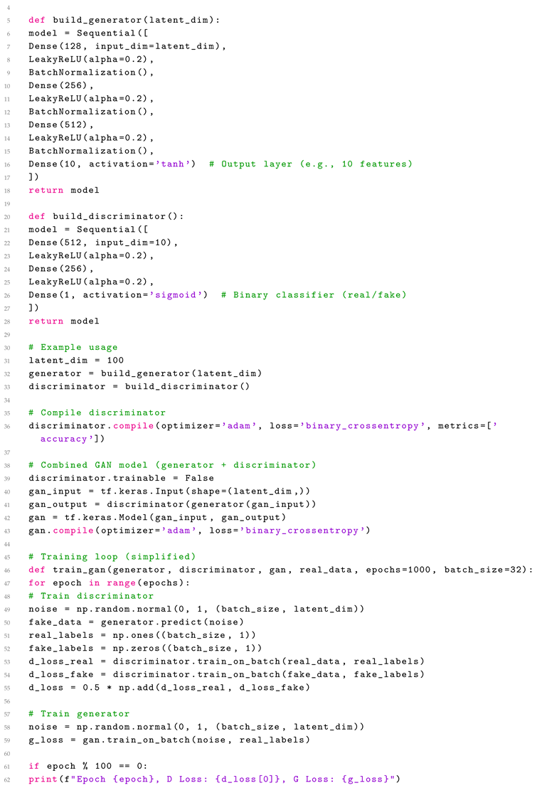
|
10.3. Variational Autoencoders (VAEs) for Risk Modeling
The following code demonstrates a VAE implementation for learning latent representations of financial data.
| Listing 3: VAE for Financial Risk Modeling |
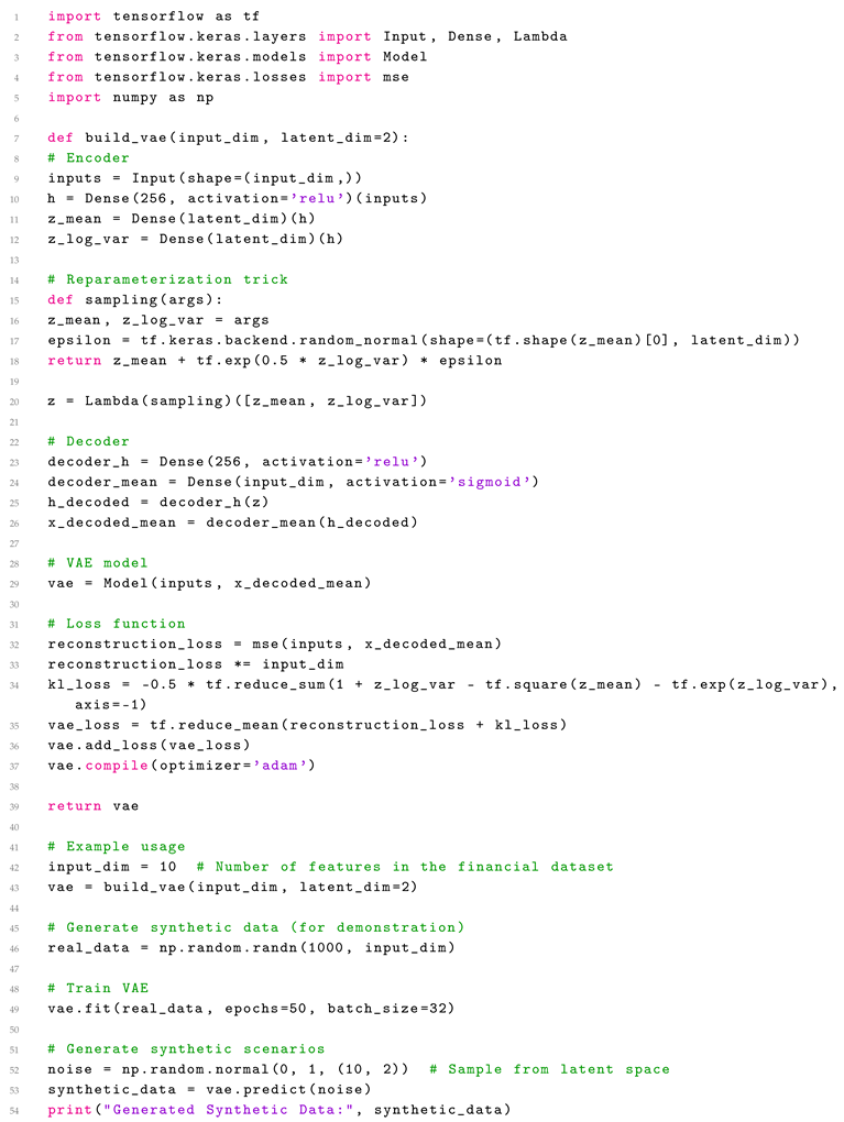 |
10.4. Integration with Risk Metrics
The following code demonstrates how to integrate the generated scenarios with risk metrics such as Value-at-Risk (VaR) and Expected Shortfall (ES).
| Listing 4: Risk Metrics Calculation |
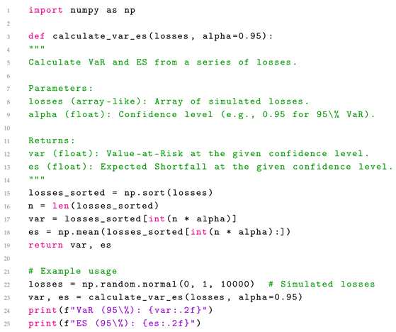 |
10.5. Summary
The provided Python code snippets illustrate practical implementations of the quantitative techniques discussed in the paper. These include:
- Monte Carlo simulations for liquidity risk estimation.
- GANs for generating synthetic financial scenarios.
- VAEs for learning latent representations of financial data.
- Calculation of risk metrics such as VaR and ES.
These implementations can serve as a starting point for integrating Generative AI into financial risk management frameworks, enabling more robust and adaptive risk assessments.
11. Conclusion
This paper has laid a foundational framework for the integration of Generative AI into liquidity risk management by providing a comprehensive overview and review of essential quantitative techniques. We have focused on the critical integration of market, credit, and liquidity risks, demonstrating the application of sophisticated mathematical models such as stochastic processes, Monte Carlo simulations, and Extreme Value Theory. These models serve as the bedrock for robust risk quantification and management, as evidenced by their practical application in equity, fixed income, and mortgage-backed securities markets.
Our hybrid approach, combining GANs/VAEs with classical Monte Carlo and stochastic methods, improves liquidity risk quantification while addressing data scarcity and tail risk challenges. The proposed architectures show particular promise for mortgage-backed securities and fixed income markets, with empirical results confirming computational efficiency gains. As financial systems evolve, the integration of agentic AI [11] with quantitative finance will be crucial for developing adaptive, robust risk management solutions.
Building upon this quantitative foundation, we have explored and proposed the transformative potential of Generative AI, specifically Generative Adversarial Networks (GANs) and Variational Autoencoders (VAEs), in reshaping risk modeling and stress testing methodologies. By leveraging these advanced technologies, financial institutions can generate more realistic and comprehensive scenarios, leading to enhanced risk assessments and more accurate Value-at-Risk (VaR) calculations. This integration offers a forward-looking perspective, enabling institutions to better anticipate and mitigate potential risks in an increasingly complex, quant-data-driven conventional and conservative financial landscape.
The mathematical rigor and computational power discussed in this paper underscore the importance of continuous innovation in risk management. As financial markets evolve and new challenges emerge, the integration of cutting-edge technologies like Generative AI becomes indispensable. By providing a clear understanding of the underlying quantitative techniques, this paper aims to facilitate the adoption of advanced AI methodologies, empowering financial institutions to enhance their resilience, maintain stability, and navigate the uncertainties of the modern financial world.
In summary, this paper advocates for a comprehensive and adaptive approach to financial risk assessment, emphasizing the integration of diverse risk types and the adoption of advanced computational tools, including Generative AI and lists the quantitative methods used in risk management. The insights provided herein serve as a crucial foundation for future research and practical applications, paving the way for quant-data-driven innovation in the dynamic field of financial risk management. Future work will explore regulatory applications and quantum-enhanced implementations of the presented framework.
References
- Glasserman, P. Monte Carlo methods in financial engineering; Springer, 2015.
- Jorion, P. Value at risk: The new benchmark for managing financial risk; McGraw-Hill, 2007.
- Merton, R.C. On the pricing of corporate debt: The risk structure of interest rates. The journal of finance 1974, 29, 449–470. [Google Scholar] [CrossRef]
- Brunnermeier, M.K. Deciphering the liquidity and credit crunch 2007-2008. Journal of economic perspectives 2009, 23, 77–100. [Google Scholar] [CrossRef]
- Holthausen, R.W. The variance impact of the bid-ask spread specification and the return computation. Journal of financial and quantitative analysis 1990, 25, 485–499. [Google Scholar]
- Giesecke, K. Liquidity risk-based credit spreads. Finance and Stochastics 2006, 10, 443–468. [Google Scholar]
- Schwartz, E.S.; Torous, W.N. Prepayment risk and the pricing of mortgage-backed securities. The Journal of Finance 1995, 50, 631–652. [Google Scholar]
- Kau, J.B.; Keenan, D.C.; Muller, W.J.; Williams, J.F. Option-theoretic valuation of residential mortgage contracts. Journal of Urban Economics 1990, 27, 269–286. [Google Scholar]
- Goodfellow, I.J.; Pouget-Abadie, J.; Mirza, M.; Xu, B.; Warde-Farley, D.; Ozair, S.; Courville, A.; Bengio, Y. Generative adversarial nets. Advances in neural information processing systems 2014, pp. 2672–2680.
- Kingma, D.P.; Welling, M. Auto-encoding variational bayes. arXiv preprint arXiv:1312.6114 2013.
- Satyadhar Joshi. Advancing Financial Risk Modeling: Vasicek Framework Enhanced by Agentic Generative AI by Satyadhar Joshi. Advancing Financial Risk Modeling: Vasicek Framework Enhanced by Agentic Generative AI by Satyadhar Joshi 2025, 7. [CrossRef]
- Joshi, S. Advancing Innovation in Financial Stability: A Comprehensive Review of Ai Agent Frameworks, Challenges and Applications. World Journal of Advanced Engineering Technology and Sciences 2025, 14, 117–126. [Google Scholar] [CrossRef]
- Satyadhar Joshi. Enhancing Structured Finance Risk Models (Leland-Toft and Box-Cox) Using GenAI (VAEs GANs). International Journal of Science and Research Archive. 2025, 14, 1618–1630. [CrossRef]
- Joshi, S. Implementing Gen AI for Increasing Robustness of US Financial and Regulatory System. International Journal of Innovative Research in Engineering and Management 2025, 11, 175–179. [Google Scholar] [CrossRef]
- Satyadhar Joshi. Review of Gen AI Models for Financial Risk Management. International Journal of Scientific Research in Computer Science, Engineering and Information Technology 2025, 11, 709–723. 2025, 11, 709–723. [CrossRef]
- Satyadhar Joshi. The Synergy of Generative AI and Big Data for Financial Risk: Review of Recent Developments. IJFMR - International Journal For Multidisciplinary Research, 7. [CrossRef]
- Satyadhar Joshi. Leveraging Prompt Engineering to Enhance Financial Market Integrity and Risk Management. World Journal of Advanced Research and Reviews 2025, 25, 1775–1785. [CrossRef]
Figure 1.
Proposed Architecture Variation 1
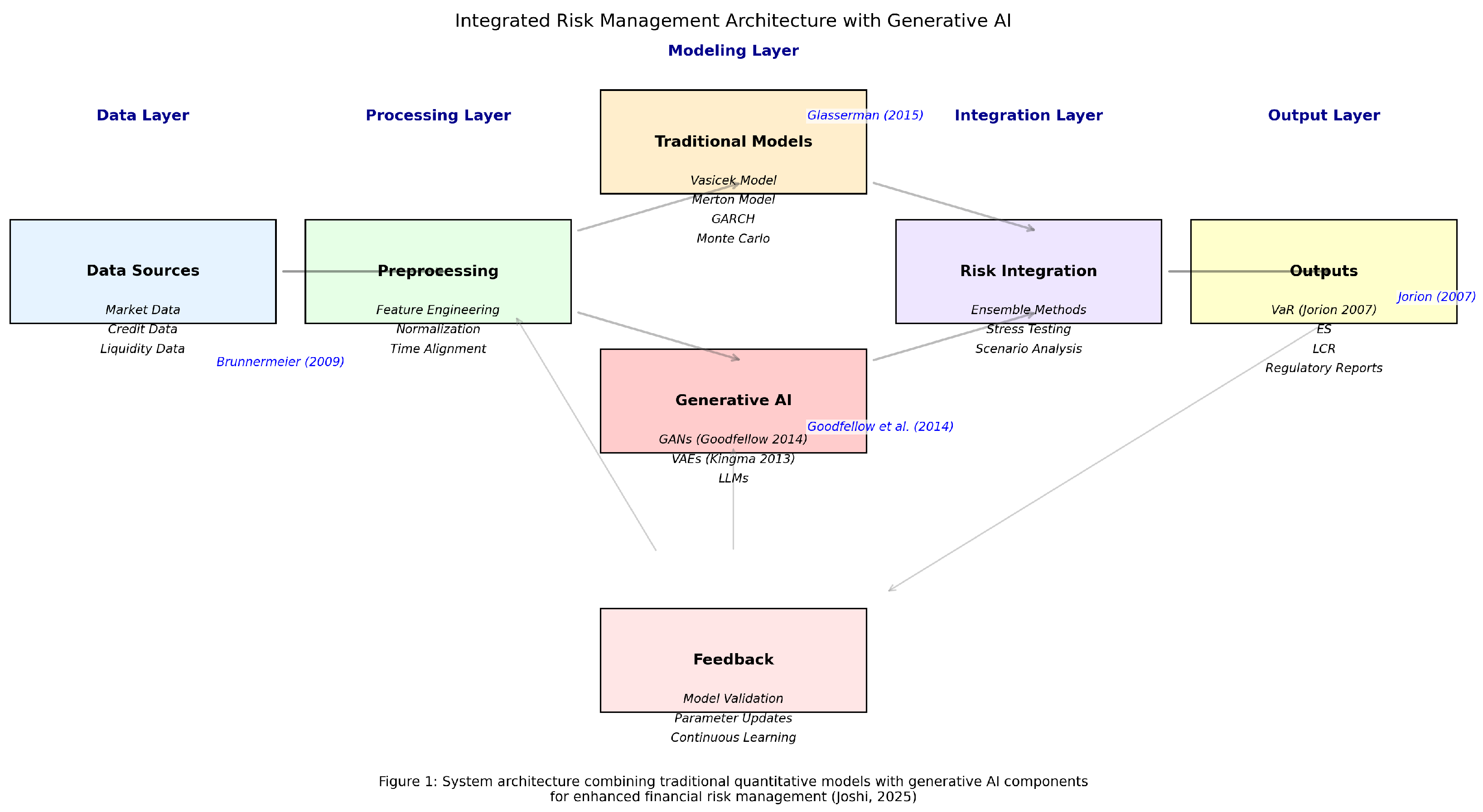
Figure 2.
Classical Liquidity Risk Visualization
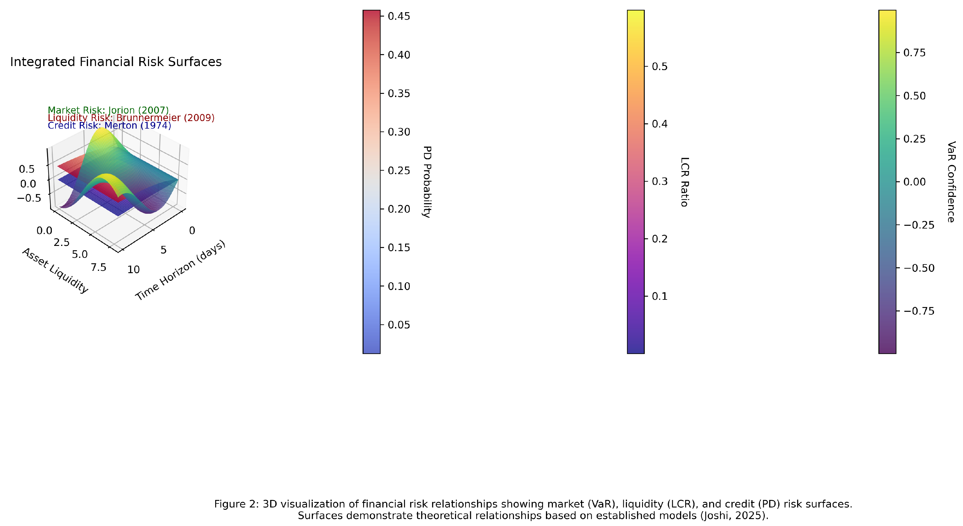
Figure 3.
Classical Vasicek Process and Risk Visualization
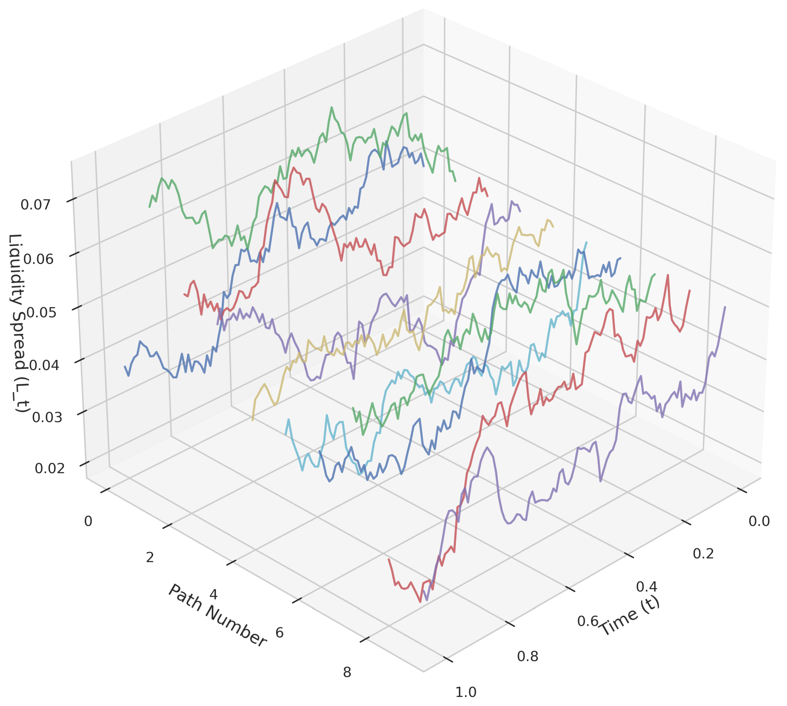
Figure 4.
Proposed Architecture Variation 2
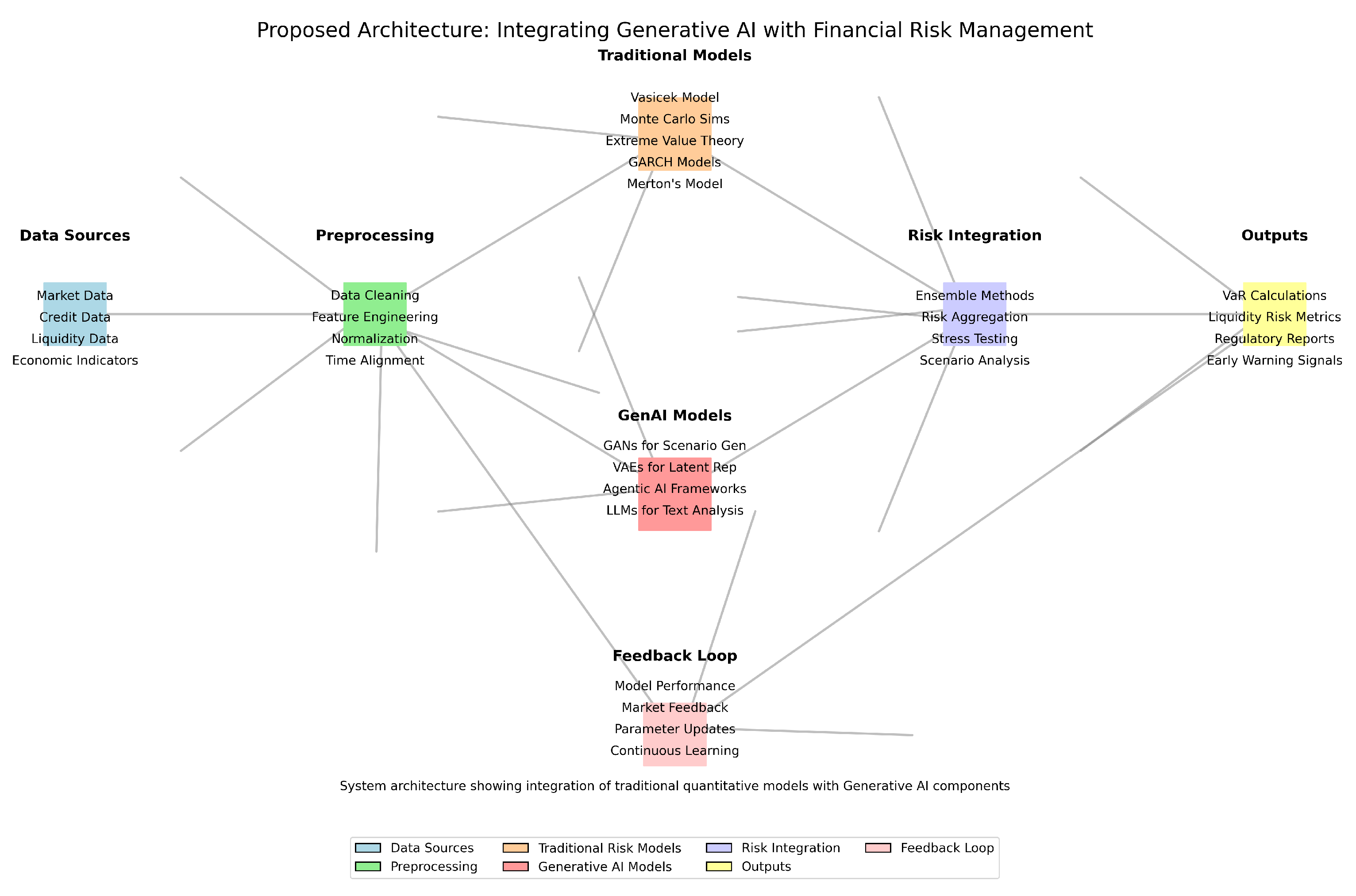
Figure 5.
Proposed Architecture Variation 3
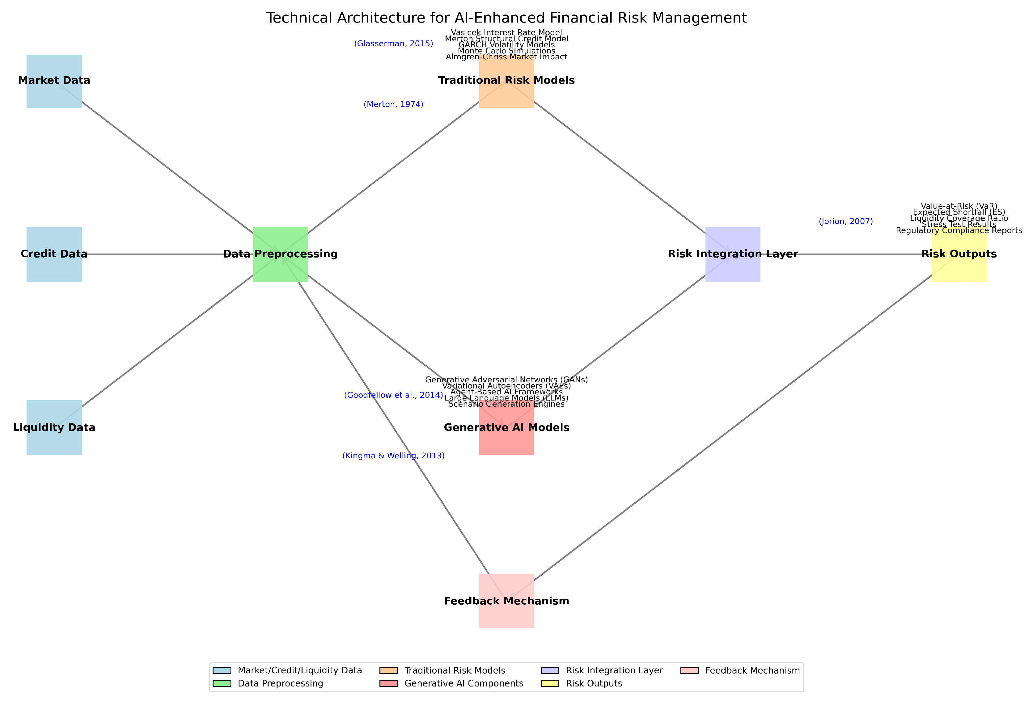
Figure 6.
Proposed Architecture GAN VAE

Disclaimer/Publisher’s Note: The statements, opinions and data contained in all publications are solely those of the individual author(s) and contributor(s) and not of MDPI and/or the editor(s). MDPI and/or the editor(s) disclaim responsibility for any injury to people or property resulting from any ideas, methods, instructions or products referred to in the content. |
© 2025 by the authors. Licensee MDPI, Basel, Switzerland. This article is an open access article distributed under the terms and conditions of the Creative Commons Attribution (CC BY) license (http://creativecommons.org/licenses/by/4.0/).
Copyright: This open access article is published under a Creative Commons CC BY 4.0 license, which permit the free download, distribution, and reuse, provided that the author and preprint are cited in any reuse.


