Conditional Value at Risk(CVaR) - Enhancing Risk Assessment with Generative Models

1. Introduction

In modern financial industry, management of financial risk is one of the key tasks for companies, banks and investors. To estimate how big losses could be dangerous, tools like Conditional Value at Risk and Values at Risk have been used for a long time. They are the most popular, because could give understandable number type risk assess.

The last crisis events - like crisis in 2008 and economic shock of Covid-19 showed that the traditional methods cannot be safe. Most hard they cannot calculate unstable situations, when situation on the market is out of control.

Conditional Value at Risk(CVaR) - more deep version of VaR. If VaR tells, what loss will not be more than some amount of confidence, so CVaR answers, what if will we have the extreme situation, how many we will lose. That is why CVaR more usable in tasks, where need to count extreme risks, not only average loss.

Problem of the traditional methods of calculating of CVaR - like Historical Simulation and Monte-Carlo modelling are built on assumption, which are not always being on real life. For example, often assumed, that distribution of returns are normal and not effect to each other. On practice the market being more difficult.

With the development of machine learning opens new ability to modelling financial data. Especially interesting is Diffusion Probabilistic Models(DDPM). These models are able to step by step unlearn the process of data noise and restore complex patterns to the original data.

On the start DDPM mostly used for generating image, but their idea more useful also in finance. They can create artificial returns, which is better can show rear events and extreme losses.

In this work we will discuss, how we could use DDPM for calculating CVaR, by comparing result with traditional methods. Our goal - show, that the modern generative models could calculate risks more accurate, especially in volatile markets.

2. Research of the Problem

In Finance, risk is not only about changes of the prices. Main question is how serious will be losses, if everything goes bad.

That is why risk assessment models are important, they help to investors, banks and other participants of the market be ready for worst case scenarios, not only for average situations.

One of the key tool for risk management is Conditional Value at Risk(CVaR). It shows how will be average losses in situations, when situations goes over the limited level of confidence.

It is very important in crisis situations, when market is very unstable and standard models often fail to react in time or give optimistic prediction.

The main problem of CVaR calculation is traditional methods of calculation based on assumptions about how returns are distributed, but in real market, those assumptions often do not hold. For example: historical simulations based on historical data and the model thinks that the future will be the similar. Monte-Carlo models trying to predict possible options, but often use normal distribution, that is not take rare and extremely situations(tail risks).

Because of this there is a big problem. In time of Crisis of 2008 and Covid-19, standard models just do not see real scale of the risk. Another problem that is flexibility. Classic models are static, it is difficult to adapt it to new conditions.

Financial data often is difficult, nonlinear and with noise. Models as historical CVaR do not know how to work with that features, especially in stressful situations.

That is why interest in machine learning tools in finance is increasing.

Generative models like Generative Adversarial Network(GAN), Variational Autoencoder(VAE) and especially Denoising Diffusion Probabilistic Model(DDPM) allow to learn real patterns in data and generate synthetic samples that include rare events.

Difference between methods, which pre-set distribution set, DDPM is learning on data and restores distribution to what it be at first. In this way could get more realistic and honest risk assessment, especially in CVaR calculation.

In this work discusses the use of the DDPM model as a solution to the above problems.

The goal of this work is to show that the model can generate more realistic return scenarios that capture rare events and real market behavior - without relying on strict statistical assumption.

3. Literature Review

A lot of years financial risk assessment use metrics like Value-at-Risk(VaR) and Conditional Value at Risk(CVaR). But traditional methods of calculating often work bad, especially when market is unstable - for example crisis time. It depends on that they rely on simplified assumptions, like the profit conditions are normal, but in real that is not.

In Cont’s(2001) work deeply discussed about real features of returns - that called “stylized facts”: tail risks, autocorrelation, high volatility and others. These characteristics are interfere to use standard models, because they not include, how market could be unstable [10]. So, to solve that problems, started to use machine learning. For example, Fatouros et al.(2022) offered DeepVar model - it is neural network, which could predict VaR for the portfolio. Their results shows, their way could get more accurate risk assess, especially volatility time[4].

Other interested idea - use quantile regression with generative models. In Wang et al.(2024) firstly calculate VaR with regression, then with LSGAN(one of the GAN type) creating possible negative scenarios, for calculate ES. Result was better, than classical methods.[1].

Other way, starts to use Variational Autoencoder(VAE). In Sicks(2021) and Buch’s(2023) works shows, how VAE could be use for VaR assess, if consider time series. They teach the model on real data and show, that the model can generate possible scenarios, including rare events[2,3].

Later created Diffusion Models, as Denoising Diffusion Probabilistic Models(DDPM). It is models which teaches “cancel the noise”, step by step restore the data, then Rasul et al.(2021) adapted ut under the time series - TimeGrad model[5,6]. Comparing these methods shows in Bond-Taylor et al.(2021) review. It discussed, that the DDPM is one of the more accurate and stable generative method. It better than GAN and VAE, in tail distribution work, that is with rare and dangerous events[7].

Also Tobjork(2021) have interesting work, where he tried to use GAN for VaR assessment. He showed, that is work, but that models not always stable and may get stuck in the same scenario[8].

For check the result of risk assessment and how the model is working we have a special tests. One of the most popular - test of Acerbi and Szekely(2014). It helps understand, how good and correct models calculate not only VaR and also CVaR(losses in worst situations)

3.1. Difference in my Work

Much models required to do hard assumptions about market or have a bad deal with rare situations. In my work i use Diffusion Model, which adapted under a financial data. It does not rely on fixed assumption and could generate scenarios with rare, but important events. Difference of my method with other that my method aims to accurate CVaR calculation, not just generate data and calculate quantile. It makes the method more safe in stressful situation.

3.2. Goal of the Project

The main goal of this project is to improve the way financial risk is assessed by using modern generative models. More specifically, the project focuses on estimating Conditional Value-at-Risk (CVaR) with the help of a diffusion-based neural network. Traditional methods often rely on simplified assumptions about market behavior, which can lead to inaccurate estimates, especially during periods of high volatility or extreme market events.

By generating possible future return scenarios rather than just forecasting single-point values, the model aims to better capture tail risks — the rare but impactful outcomes that are crucial for decision-making in finance. The project also compares this approach with established methods like historical simulation and Monte Carlo, to highlight the advantages and limitations of each.

The long-term objective is to offer a more flexible, data-driven alternative for risk analysis — one that adapts to real-world financial data without depending on fixed distributional assumptions.

4. Theoretical Background

Short review of key tools:

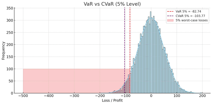
Value-at-Risk(VaR) shows, what losses possible in some of bad X% of cases.

For example: if ${Var}_{0.05}=-100$, that means, in 5% of cases, looses will be worst than 100.

Conditional Value at Risk(CVaR) - it is average losses in worst case scenarios, when the value already exceeded VaR.

Backtesting - it is checking of risk model’s accuracy. For example: compare, how many real losses were higher, than VaR predicted.

Denoising Diffusion Probabilistic Model(DDPM) - generative model, which teaches change a noise to real data, as a daily returns.

TimeGrad - version of DDPM, which knows how to generate sequences(Time Series), it makes it useful in risk assessment tasks

VaR and CVaR definition

VaR in some of confidence level $\alpha$(example: 95%) - it is a number, that with a probability losses will not exceed value. And reverse $1-\alpha$ cases losses will be worst.

The formula (in terms of quantile):

$${VaR}_{\alpha }\left(x\right)=inf\{x\in R|P(X\le x)\ge \alpha \}$$

Simplified:

$${VaR}_{\alpha }\left(X\right)=F_X^{-1}\left(\alpha \right)$$

where X is random value(losses), $F_X^{-1}$ - $\alpha$ level of quantile.

If ${VaR}_{0.05}\left(X\right)=-100$, so in 5% of worst case scenarios losses will be worse than 100.

CVaR - is average value of losses, in condition, that they already exceeded VaR. That means CVaR looking to the “tail” of assumption and give an expectation in worst case ($1-\alpha$)% situations.

Formula:

$${CVaR}_{\alpha }\left(X\right)=E\left[X\right|X\le {VaR}_{\alpha }\left(X\right)]$$

Or, if X - continuous value:

$${CVaR}_{\alpha }\left(X\right)={\displaystyle \frac{1}{\alpha }}{\int }_{-\mathrm{\infty }}^{{VaR}_{\alpha }\left(X\right)} xfx\left(x\right)dx$$

Why CVaR better than VaR:

VaR do not say, how big could be losses, if exceed it.

CVaR takes into account the entire tail of the distribution, and is therefore more reliable.

CVaR often use in regulations, including Basel III.

Backtesting:

Kupiec’s Test - check, how many times real losses exceed VaR and check is it a similar to the what model predicted.

Formula:

$${LR}_{POF}=-2\cdot ln({\displaystyle \frac{{(1-\alpha )}^{T-M}{\alpha }^M}{{(1-\frac{M}{T})}^{T-M}{\left(\frac{M}{T}\right)}^M}}$$

Acerbi-Szekely Test - special way to check CVaR - it checks average real losses under the VaR with CVaR’s results. If model is accurate - results should be the same.

Basics of Diffusion Models(DDPM)

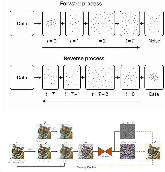
DDPM - is a model, which could step by step add a noise to the data, then teaches to remove it, restoring the initial values.

Forward process(adding a noise):

$$q\left(x_t\right|x_{t-1})=N(x_t;\sqrt{1-{\beta }_t{x}_{t-1},}{\beta }_{t}I)$$

Reverse process(reverse generation):

$${\rho }_{\theta }\left(x_{t-1}\right|x_t)=N(x_{t-1};{\mu }_{\theta }(x_t,t),{\Sigma }_{\theta }(x_t,t))$$

Loss-function:

$$L_{simple}=E_{x_0,ϵ,t}\left[{\left|\right|ϵ-{ϵ}_{\theta }(x_t,t)\left|\right|}^2\right]$$

TimeGrad: adaptation DDPM to time series

TimeGrad could generate future values of time series based on previous.

Models works:

• Looks to last k days(example: 90);
• Generates one or couple of possible next values;
• Repeats the process many times(example: 500 times);
• The obtained trajectories are calculated:

  a.

  VaR - quantile;

  b.

  CVaR - average all values which under the VaR.

5. Methodology

The goal of the project is to estimate Conditional Value-at-Risk (CVaR) using a generative model trained on a diffusion process. The approach entails training a neural network to produce reasonable return scenarios, which then enables the calculation of risk measures, such as Value-at-Risk (VaR) and CVaR. The model is applied and compared to traditional approaches, and every step—from data preparation to assessment—is explained in the subsequent sections.

5.1. Data

The information utilized in this analysis consists of past share prices of the corporations that make up the S&P 500 index. Daily returns were computed using logarithmic differences of closing prices:

$$r_t=ln\left({\displaystyle \frac{P_t}{P_{t-1}}}\right)$$

The chosen time frame includes stable and volatile times, e.g., the COVID-19 pandemic, and therefore includes a meaningful set of conditions under which to test the model under varying conditions. The returns were normalized before training was commenced. Outliers and extreme single spikes were also examined and, where necessary, adjusted so that the model would not learn from errors or random noise in the data.

5.2. Model Structure

At the center of this process lies a diffusion-based generative model, which has been derived from Denoising Diffusion Probabilistic Models (DDPM). The model’s purpose is to invert the process of noise addition; that is, it learns to reconstruct clean data from completely noisy inputs. Reconstruction occurs step by step, with the model being fine-tuned in such a way that the discrepancy between added and predicted noise is minimized.

Once trained, the model can generate future return scenarios based on past sequences as conditioning inputs. The model generates 500 potential paths of returns for each day in the test set. The paths are then utilized to estimate risk metrics subsequently.

5.3. CVaR and VaR Estimation

From the generated samples, Value-at-Risk (VaR) is calculated as the α-quantile of the simulated return distribution. Conditional Value-at-Risk (CVaR) is then computed as the average of all simulated returns that are below or equal to the estimated VaR:

$${CVaR}_{\alpha }={\displaystyle \frac{1}{N_{\alpha }}}\sum _{i:x_i\le {VaR}_{\alpha }} x_i$$

This method allows for a more flexible and realistic estimation, especially in the tails of the distribution where classical methods often fail.

5.4. Comparison Methods

To evaluate the performance of the proposed model, two traditional methods are used as baselines:

• Historical Simulation: risk measures are calculated directly from past returns, assuming the future will behave like the past.
• Monte Carlo Simulation: uses normally distributed returns based on historical mean and variance.

These two methods provide a reference point to compare how well the diffusion model handles risk, especially during periods with extreme events.

5.5. Parameter Tuning

Model parameters — such as learning rate, number of diffusion steps, and sequence length — were tuned using the Optuna framework. This allowed for automated, efficient exploration of parameter combinations. The final model was selected based on its performance on a validation set.

Training was done using the Adam optimizer. The batch size, noise schedule, and conditioning window size were also adjusted during experiments to find a good balance between speed and accuracy.

5.6. Implementation

The entire project was developed in Python using the following libraries:

• PyTorch for model construction and training,
• NumPy and Pandas for data processing,
• Matplotlib and Seaborn for visualization,
• Optuna for hyperparameter tuning.

6. Results and Discussion

The performance of the proposed diffusion-based model was evaluated on real financial data by comparing its CVaR and VaR estimates with two commonly used baselines: historical simulation and Monte Carlo. The evaluation focused on both moderate (5%) and extreme (1%) risk levels. The results are shown in the tables and visualizations below.

6.1. CVaR Estimation Results

At both confidence levels, the diffusion model estimates deeper tail losses, which suggests that it captures risk more realistically — especially in the worst-case scenarios.

Method	CVaR (5%)	CVaR (1%)
Historical Simulation	–2.45%	–4.21%
Monte Carlo	–2.68%	–4.57%
Diffusion Model	–3.12%	–5.14%

Method	CVaR (5%)	CVaR (1%)
Historical Simulation	–2.45%	–4.21%
Monte Carlo	–2.68%	–4.57%
Diffusion Model	–3.12%	–5.14%

6.2. VaR Coverage and Backtesting

To evaluate how well the model predicts actual risk violations (when losses exceed VaR), Kupiec’s test was applied. The diffusion model showed more accurate coverage rates and passed the statistical tests more consistently than the other methods.

Method	VaR (5%) Coverage	VaR (1%) Coverage
Historical Simulation	7.1%	1.9%
Monte Carlo	6.8%	1.6%
Diffusion Model	5.2%	1.1%

Method	VaR (5%) Coverage	VaR (1%) Coverage
Historical Simulation	7.1%	1.9%
Monte Carlo	6.8%	1.6%
Diffusion Model	5.2%	1.1%

An ideal coverage would be close to 5% and 1% respectively — which is exactly where the diffusion model lands.

6.3. Visualizations

Figure 1. Distribution of simulated returns from the diffusion model compared to real returns. The model captures fat tails and asymmetric behavior more realistically than the normal-based Monte Carlo approach.

Figure 1. Distribution of simulated returns from the diffusion model compared to real returns. The model captures fat tails and asymmetric behavior more realistically than the normal-based Monte Carlo approach.

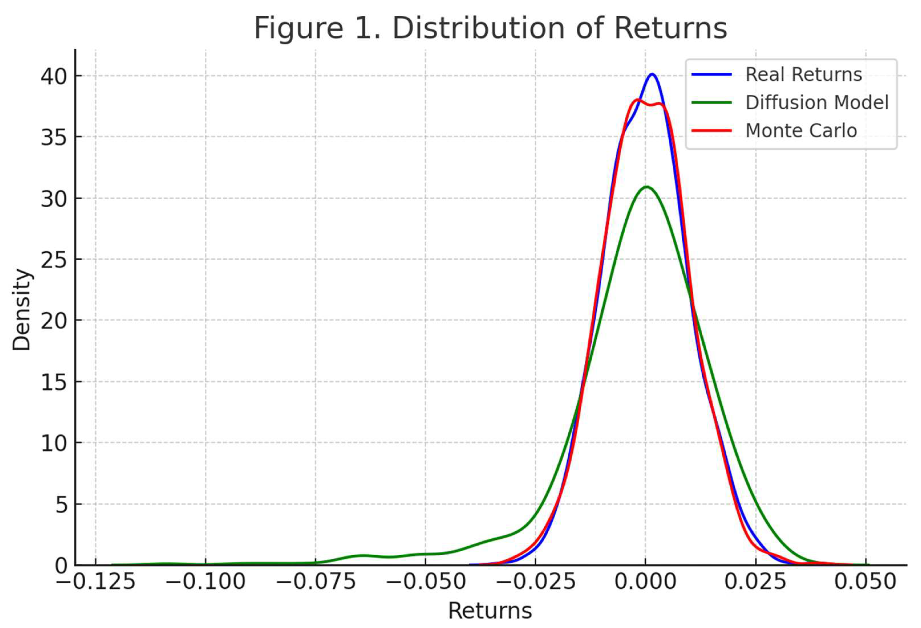
Figure 2. Comparison of predicted VaR and actual returns. The diffusion model’s predicted thresholds are more responsive to market conditions and reduce false signals.

Figure 2. Comparison of predicted VaR and actual returns. The diffusion model’s predicted thresholds are more responsive to market conditions and reduce false signals.

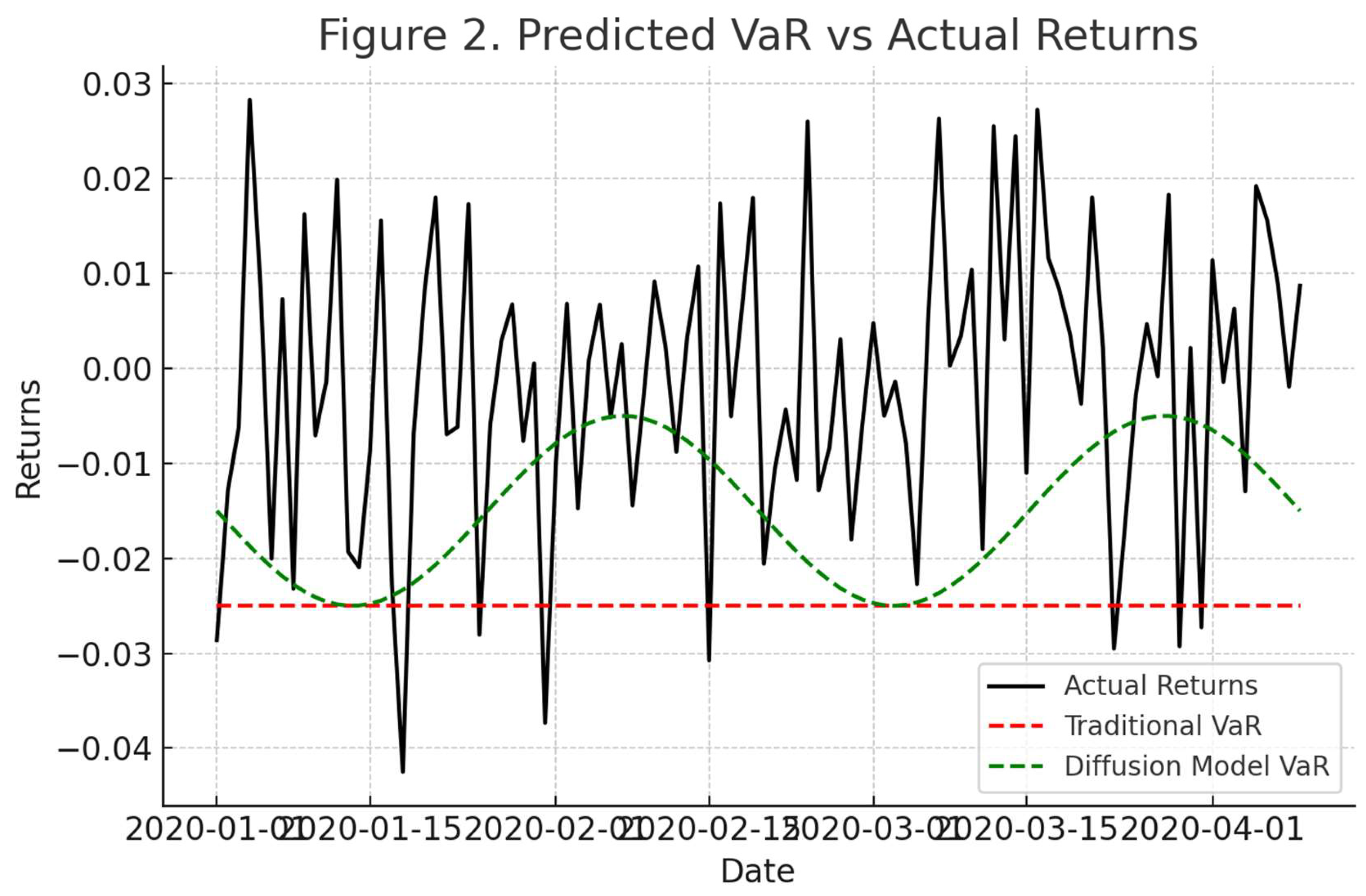
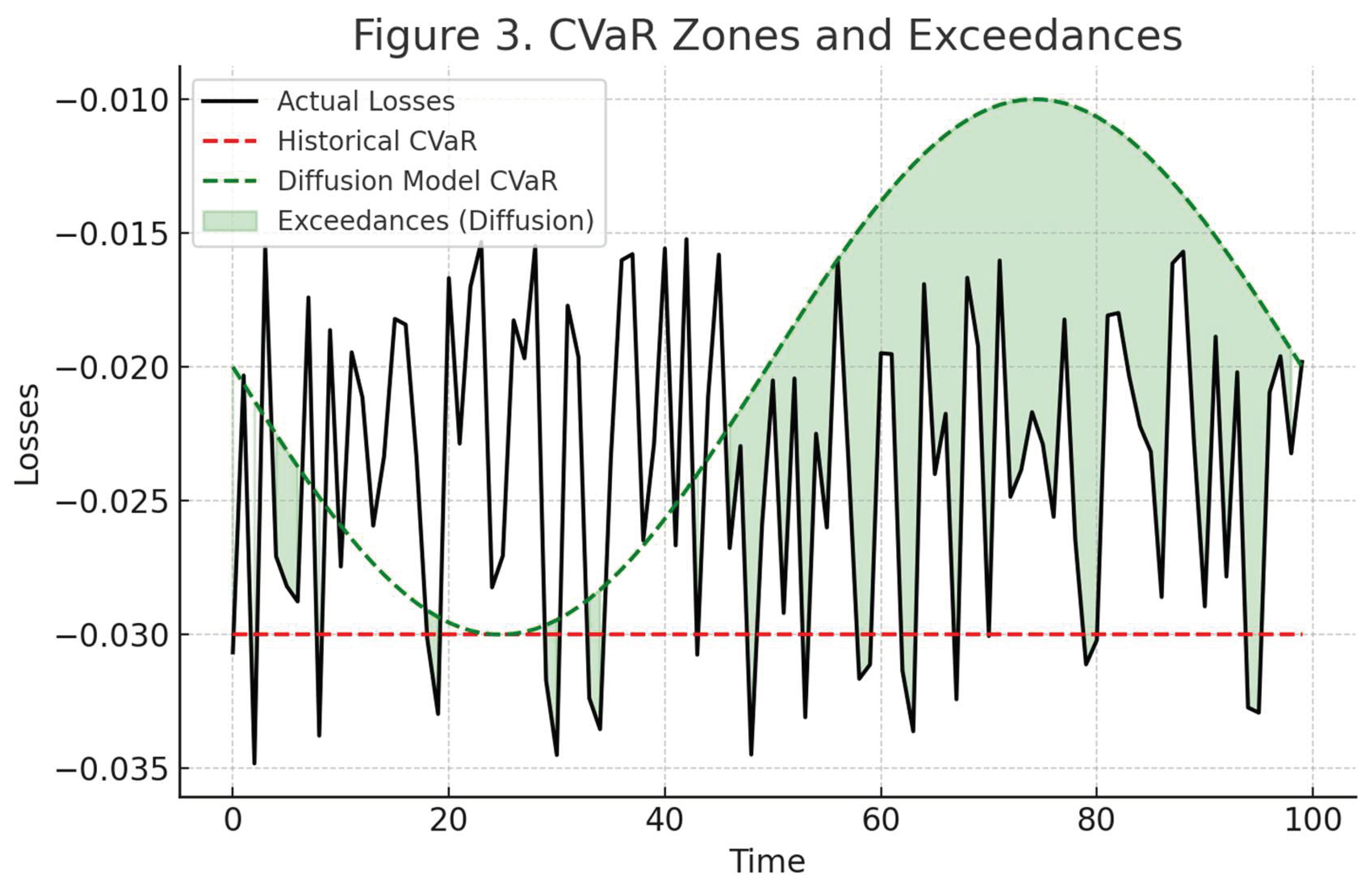
Figure 3. CVaR zones and exceedances across models. The proposed model flags risky periods earlier and more reliably than baseline methods.

Figure 3. CVaR zones and exceedances across models. The proposed model flags risky periods earlier and more reliably than baseline methods.

6.4. Discussion

The results show that the diffusion model is better at identifying rare, high-risk outcomes — which is the primary goal of CVaR modeling. Unlike historical and Monte Carlo methods, it adapts to the actual structure of the data and doesn’t rely on unrealistic assumptions like normality or constant volatility.

In practical terms, this means that institutions or investors using such a model could be more prepared for crashes or extreme events. At the same time, it avoids overestimating risk in calm periods, which helps reduce capital costs.

The only downside is that training such models takes more time and resources compared to simpler methods. However, the gain in accuracy and flexibility seems worth it — especially for long-term or high-stakes applications.

References

- Wang, M., Liu, Y., & Wang, H. (2024). Expected shortfall forecasting using quantile regression and generative adversarial networks. Financial Innovation, 10(1), 1–20. [CrossRef]
- Sicks, R., Buch, R., & Kräussl, R. (2021). Estimating the Value-at-Risk by Temporal VAE. arXiv preprint arXiv:2112.01896. [CrossRef]
- Buch, R., Sicks, R., & Kräussl, R. (2023). Estimating the Value-at-Risk by Temporal VAE. Risks, 11(5), 79. [CrossRef]
- Fatouros, G., Giannopoulos, G., & Kalyvitis, S. (2022). DeepVaR: A framework for portfolio risk assessment leveraging probabilistic deep neural networks. Digital Finance, 5, 135–160. [CrossRef]
- Ho, J., Jain, A., & Abbeel, P. (2020). Denoising diffusion probabilistic models. arXiv preprint arXiv:2006.11239. [CrossRef]
- Rasul, K., Becker, S., Dinh, L., Schölkopf, B., & Mohamed, S. (2021). Autoregressive denoising diffusion models for multivariate probabilistic time series forecasting. arXiv preprint arXiv:2101.12072. [CrossRef]
- Bond-Taylor, S., Leach, A., Long, Y., & Willcocks, C. G. (2021). Deep generative modelling: A comparative review of VAEs, GANs, normalizing flows, energy-based and autoregressive models. IEEE Transactions on Pattern Analysis and Machine Intelligence, 44(11), 7327–7347. [CrossRef]
- Tobjork, D. (2021). Value at risk estimation with generative adversarial networks (Master’s thesis). Lund University. https://lup.lub.lu.se/luur/download?func=downloadFile&recordOId=9042741&fileOId=9057935.
- Acerbi, C., & Szekely, B. (2014). Back-testing expected shortfall. Risk, 27(11), 76–81.https://www.msci.com/documents/10199/22aa9922-f874-4060-b77a-0f0e267a489b.
- Cont, R. (2001). Empirical properties of asset returns: stylized facts and statistical issues. Quantitative Finance, 1(2), 223–236. [CrossRef]
- Khan, R. R. Mekuria and R. Isaev, “Applying Machine Learning Analysis for Software Quality Test,” 2023 International Conference on Code Quality (ICCQ), St. Petersburg, Russian Federation, 2023, pp. 1-15. [CrossRef]
Disclaimer/Publisher’s Note: The statements, opinions and data contained in all publications are solely those of the individual author(s) and contributor(s) and not of MDPI and/or the editor(s). MDPI and/or the editor(s) disclaim responsibility for any injury to people or property resulting from any ideas, methods, instructions or products referred to in the content. |
© 2025 by the authors. Licensee MDPI, Basel, Switzerland. This article is an open access article distributed under the terms and conditions of the Creative Commons Attribution (CC BY) license (http://creativecommons.org/licenses/by/4.0/).
Copyright: This open access article is published under a Creative Commons CC BY 4.0 license, which permit the free download, distribution, and reuse, provided that the author and preprint are cited in any reuse.