
Submitted:
26 February 2025
Posted:
27 February 2025
You are already at the latest version
Abstract
The remote sensing community has been calling for more precise monitoring of ecosystems, environmental changes, and natural resource management, including forest management. It is crucial to monitor metrics like the overall biomass and the total area index, among others. A vast number of experiments and an accurate scattering model are required to acquire the parameters of interest. Advances in the field of radar interferometry have introduced two additional quantities containing target information. These two numbers represent the interferogram phase and the correlation coefficient. To understand these values about the target's parameter of interest, the interaction of waves with vegetation particles is crucial. This work presents a discrete interferometric model of a random medium layer for use in radar interferometry applications. The model establishes the relationship between radar interferometry and forest biophysical parameters. With the help of correlation analysis, the value of one variable can be estimated given the value of another. Correlation analysis contributes to the understanding of medium behavior, and it decreases the range of uncertainty within a random medium. In this study, the modelling approach of the discrete interferometric model is introduced. The aim here is to compare the approaches with simulation results and generalize the theoretical works.
Keywords:
ecosystems
; interferometric model
; remote sensing
; vegetation
1. Introduction
The extraction of vegetation characteristics from radar data has emerged as a significant concern in remote sensing. The demand for ecosystem monitoring, natural resource management, including forests, and environmental change assessment is rising. A substantial quantity of experiments is necessary to acquire important data. Diverse models are employed to achieve correlation, phase, and coherence attributes. [1] and [2] employ models to ascertain correlation features. It is claimed that certain models yield consistent outcomes. Additionally, other parameters are thought to influence the features and sensitivity analysis.
This study seeks to examine and model our discrete interferometric framework for a layer of stochastic medium. The software will assist with simulation and outcomes. Methods for extracting vegetation characteristics and the underlying ground surface topography from InSAR data are proposed in [1,2,3]. The modeling procedure encompasses the simulation of electromagnetic scattering and radar processing that constitute the InSAR observations. Subsequently, characteristics for vegetation and terrain are selected for estimation. Subsequently, parameter discrepancies are evaluated against the performance of InSAR sensors, and parameter estimations derived from InSAR data are presented and juxtaposed with real-world observations. The literature review indicates that are the initial studies employing mathematics to elucidate InSAR observations through the physical characteristics of vegetation, such as scatterer amplitude, extinction coefficient, incident angle, baseline distance, and the height of the ground surface or the depth of the vegetation layer. Treuhaft et al. in 2004 provides further information to Treuhaft et al. in 1996 regarding the correlation and power characteristics [1,2]. The theoretical work in [1] is analyzed in [2], leading to a mathematical generalization. To determine the potential applications of vegetated terrain, the vegetation environment is transformed into a stochastic medium model, with its statistical characteristics correlated to its physical attributes. The impacts of alterations in radar data are noted.
In the microwave spectrum, the predominant sensors utilized are radiometers and radars. Radar functions as a distance measurement instrument, exemplified by altimeters, or for imaging purposes, as seen in Side Looking Airborne Radar (SLAR) and Synthetic Aperture Radar (SAR). SAR is a radar system that generates a highly focused effective beam through sophisticated processing of radar data. Consequently, image acquisition is independent of natural light, enabling the capturing of photographs at night. The little atmospheric absorption ensures that cloud cover does not obstruct observations.
SAR signal processing involves coherent phase correction that rectifies the particular phase shift history of the signal reflected from a designated location on the ground, accounting for the velocity of the aircraft (radar). From this compensation, only returns from that moment are effectively included across the full observation period. The necessary phase adjustment can be inferred from the anticipated phase history of a ground return to an aerial radar [4,5,6].
Interferometric synthetic aperture radar technology, abbreviated as InSAR or IfSAR, is employed in remote sensing and geodesy. This geodetic technique employs variations in wave phases returning to the satellite or aircraft to generate digital elevations or surface alterations from two or more synthetic aperture radar images. It is applicable in structural engineering for monitoring structural stability and subsidence, as well as for geophysical surveillance of natural hazards such as earthquakes, volcanoes, and landslides.
2. Experimental Methods
2.1. Theoretical Background
Numerous studies and applications exist for InSAR and other radar technologies. Geometry, radar bandwidth constraints, and limited signal-to-noise ratios may result in ambiguity [6,7,8,9]. Current implementations are primarily constrained by the precision of aircraft attitude knowledge, which will also influence future uses. The theory and design of InSARs were addressed in [6,7,8,9,10]. These studies delineate the derivation of signal statistics, an efficient estimator for the interferometric phase, and the requisite equations for calculating the height-error budget. Additionally, they provide a set of design guidelines for enhancing InSAR performance. It was determined that interferometric mapping offers a high-resolution topographic system capable of functioning effectively in challenging topographical conditions. It develops a model that incorporates both radar system characteristics and scene scattering parameters, utilizing it to analyze observations in a forested region with varying coherence. Thus, coherence is observed to be responsive to temperature but not to the influence of wind. The interferometric height discontinuity exhibited strong correlation with a dense forest.
SAR systems are recognized for producing distinctive images that depict the electrical and geometrical characteristics of a surface under almost all weather situations, hence providing its illumination. Subsequent InSAR systems were developed to capture the complex amplitude and phase information of each antenna, thereby eliminating the challenges associated with inverting amplitude fringes for topographic retrieval.
2.2. Treuhaft’s Model
To examine the sensitivity of an interferometric SAR response to the physical characteristics of forest stands, [9,10] employ a coherent scattering model for tree canopies. The scattering phase center of the pixel, determined by InSAR, is characterized through the concept of an equivalent scatterer representing a collective of scatterers inside a pixel, which corresponds to the vegetative components of arboreal structures. A first-order scattering model applied to fractal-generated tree structures is integrated with a newly established equivalency relation between InSAR and the correlation coefficient of forest stands, determined numerically, to develop the model. The wavelength, slant range, baseline distance between antennas, antenna orientation, and the height of the scattering phase center above a reference line all influence the phase of the interferogram. Moreover, the requisite statistics for height estimation utilizing InSAR can be acquired by comprehending the frequency correlation characteristics of radar backscatter. The height estimation of a distributed target is unaffected by baseline distance and relies solely on the comparable frequency decorrelation bandwidth. [8,9,10] elucidates the methodology for evaluating extinction, physical height, and the height of the scattering phase center of a closed, homogeneous, semi-infinite canopy through the characteristics measured via InSAR.
To assess biomass, leaf area index, and vegetation type, it is essential to evaluate both the topographic attributes of the plant and its characteristics in relation to vertical height above the ground. This is referred to as vertical structure. While polarimetry mostly responds to the shape and alignment of plant scatterers, radar interferometry predominantly reacts to the spatial arrangement of vegetation. Consequently, polarimetric interferometry, which involves interferometry across all possible polarization channels at each end of the baseline, is far more sensitive to the arrangement of oriented objects in a vegetated landscape than either polarimetry or interferometry used independently. This intricate cross-correlation is articulated through three physical models for vegetation parameters in [1,2,8,9]: (1) a randomly oriented volume; (2) a randomly oriented volume with ground return; and (3) an oriented volume. It is concluded that parameter estimation using less constrained and more realistic models will be feasible with fully polarimetric interferometry. Consequently, vertical-structure parameters obtained from polarimetric interferometry may exhibit more accuracy than those estimated from the combination of zero-baseline polarimetry and interferometry.
The primary characteristics of a forest random medium are biomass and vertical structure. This study [8,9] employs a uniform, random-volume model of the forest medium to assess the sensitivity of power and interferometric synthetic aperture radar to tree height and vegetation density, considering extinction along with speckle and thermal noise. Calculations indicate that radar power exhibits more resilience to structural and biomass interference than InSAR coherence and phase. Figure 1 demonstrates that InSAR-based methodologies for structure and biomass assessment surpass SAR power in scenarios of elevated biomass and dense vegetation [1,2,8,9]. As tree height increases, InSAR coherence diminishes and attains a saturation threshold beyond 40 meters. The InSAR phase continues to increase without attaining saturation. The lengths of the vectors representing each vegetation element are proportional to the vegetation density to accommodate for attenuation at every height. If vegetation elements are distributed vertically, the overall interferometric amplitude is inferior to the zero baseline, and the coherence is below 1. The extreme vegetation components constitute the comprehensive interferometric phase. The interferometric phase elevates while the interferometric coherence diminishes as canopy heights grow. The biomass is directly proportional to the x-axis according to the fundamental model’s assumptions.
Power, phase, and coherence are found to be proportional to the terms in (1) [3].
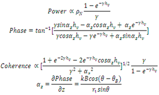
where α_z denotes the partial derivative of the interferometric phase with respect to altitude above the ground surface. To maintain simplicity, variations in absorption are neglected for a constant canopy height of 30 m, positing that alterations in ρN (vegetation scatterer number density) are the sole contributors to extinction variations, rather than fluctuations in Im (absorption). Assuming constant absorption, the extinction coefficient is considered proportional to biomass and solely reflects variations in density.
The augmentation of power is associated with the elevation of the trees. As the signal is increasingly influenced by elevated canopy heights and a diminished portion of the forest’s vertical expanse contributes, the InSAR coherence correspondingly rises with extinction. The augmentation in InSAR phase is additionally attributed to contributions from higher altitudes [1,3]. It is reasonable to anticipate that biomass will increase with heightened vegetation density or height. A comparison of the unique coherence behavior in Figure 2 with efforts to develop novel biomass patterns is advised. Instead of representing biomass through raw coherence and phase measurements, the figures emphasize the advantage of deriving structural aspects from the interferometric data. Even at minimal extinctions, InSAR surpasses power in detecting height variations. Furthermore, it is posited that, with the exception of the lowest biomasses, the majority of biomass values at L- and C-band frequencies exhibit greater sensitivity than power. If the primary distinction between stands is density, then extinctions diminish at lower frequencies, such as P-band, which may enhance radar power for the assessment of low biomass, low-density standards.
InSAR observations demonstrate superior sensitivity to height fluctuations compared to power. The non-uniqueness of signatures in data formats and the associated challenges of inversion impact both power and InSAR observations similarly. Generally, structure exhibits more sensitivity to InSAR measurements than power. The model examined in this work indicates that tree height and the extinction coefficient cannot be uniquely ascertained from a solitary InSAR measurement of coherence and phase. Nevertheless, the literature contains examples that illustrate the distinctive capability to ascertain tree height, extinction, and many structural profile features through the integration of multi-baseline, multi-polarization, or multi-frequency InSAR. The modeling process encompasses the simulation of electromagnetic scattering and radar processing that produce InSAR observations, the identification of vegetation and topographic parameters for estimation, the assessment of parameter errors relative to InSAR instrumental performance, and the demonstration of parameter estimation using InSAR data, followed by a comparison with ground truth. Three metrics were assessed: the SAR backscattered power, the cross-correlation phase, and the cross-correlation amplitude. To characterize the vegetation and surface topography, the following parameters were identified: the elevation of the underlying ground surface, the depth of the vegetation layer, the vegetation extinction coefficient (power loss per unit length), and a parameter representing the product of the average backscattering amplitude and scatterer number density.
Figure 2 illustrates the two antennas employed in the InSAR technology, wherein transmitted microwave radiation is reflected from the Earth’s surface and received by these antennas. These antennas represent the termini of an interferometric baseline, shown as B in the picture. B is equivalent to the positional difference between receivers 2 and 1, R2 - R1. For the sake of simplicity, both the baseline and the ground surface are assumed to be horizontal. Two receivers and one transmitter are applicable for usage aboard aircraft. The observed vegetation area extends from z=0, representing the ground surface height, to z0+hv, where hv denotes the depth of the vegetation layer. The intricate relationship of the fields obtained at the extremities of the baseline is the primary form of interferometric data. Equating the arguments of the range resolution functions yields the final expression for the cross-correlation.
can be re-written as;
Where
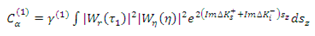
In (4), the weight function Wη is included, where η is the azimuthal angle measured in the horizontal plane. The Wη function results from the process of synthesizing the aperture.”
The range resolution function Wr is given by:
where the transmitted pulse, with Fourier transform G(ω), is centered at time t=0, and ω0 is the center frequency of the transmitted signal. Wr is symmetric about its maximum, which occurs when its argument is zero.
Let the far field from transmitter A, on the interface of the layer of random medium electric field is shown in Figure 3.
where is wave number, is the antenna pattern of the transmitter, and R is the distance. [11,12] find the correlation of the fluctuating component of the scattering field as,
where ese (x,s) is the scattered field at x due to a scatterer at s and ρ(s) is the density of particles.
From (8), the correlation of the field is found as:
where is assumed.
Figure 4 illustrates the four trajectories of the bi-static field. These four options manifest as reflection coefficients during the correlation of fields. The aforementioned equations and Figure 3 and Figure 4 yield the four routes of the bi-static field for a narrow-band signal.

where α=1 for the trunk, α=2 for the branch and α=3 for leaves.


Where
where A is the area and,
If we let θs = θi, then Im ▁f(0) = Im▁( f)(i) = Im ▁f hence
Thus (2.13) takes the form
An analysis of the terminology in Treuhaft’s Model and Seker & Lang’s Model revealed that both are identical. In Seker’s model, the parameters of the weight and range resolution functions are not displayed. Furthermore, the expression is designated as sz. The particle density is assumed to be constant in both equations. The symbols (r1-r2) and (R1-R2) in both equations appear identical, as do the notations ,
Without the arguments, correlation eq. can be given as:
Comparing both models, the only parameters needed to equate are the terms
and Since it isknown that the scattering amplitude, is equal to term. From here, the equivalence below can be obtained.
2.3. Reflection Coefficient Contribution
The contributions of reflection coefficients to correlation equations can be ascertained from the research in [9]. Models for polarimetry and interferometry, including polarimetric interferometry, can be cohesively created by establishing a general complex cross-correlation. This study introduces three physical models that elucidate the intricate cross-correlation concerning vegetation parameters: (1) an oriented volume, (2) a randomly oriented volume with ground return, and (3) an orientated volume. The initial two models incorporate the following elements: vegetation height, extinction coefficient, underlying topography, and an extra component derived from the electrical properties and roughness of the terrain. The refractivity, extinction coefficients, and backscattering characteristics of waves traveling through the vegetative volume establish further parameters for the oriented volume. These models indicate a 1% probability for each meter of variation in vegetation height in the polarimetric {HHHH/VVVV} (H ̂ to V ̂, transmit and receive, polarimetric power ratio) and the interferometric cross-correlation amplitude. The study asserts that parameter estimation can be enhanced in realism and accuracy by the application of single-baseline and multi-baseline totally polarimetric interferometry.
The broadest cross-correlation, appropriate for both polarimetry and interferometry, is:
where is the receive polarization at end 1 of the baseline, located at , and is the vector signal received at , due to a wave transmitted at the polarization . is the receive polarization at end 2 of the baseline, while is the transmit polarization, which induces the return received at end 2 of the baseline. The ensemble average angle brackets in (26) indicate the average overall statistical properties of the terrain which affect the signals.
In (26), the transmit and receive polarizations , and can be arbitrary, linear, complex (e.g., for circular polarization) combinations of . The polarization and baseline conventions describing “interferometry” (INSAR), “polarimetry” (POLSAR) and “polarimetric interferometry” (POLINSAR) are given in [9].
2.4. Homogeneous Randomly Oriented Volume
The fundamental vegetation model, characterized by a homogeneous randomly oriented volume, serves as a valuable foundation for considering INSAR, POLSAR, and POLINSAR. Each model scenario presented in [9] includes a summary of its parameters and observations. The decrease in specular amplitude caused by roughness is represented by the term Γrough.
where σH is the expected Gaussian-distributed ground heights are standardly derivable. Although it always multiplies the reflection coefficient, the ground roughness term is added for completeness, therefore by itself, σH will not appear as a parameter. The whole path length is included in the equal phases of the ground-volume and volume-ground components. The length of this path, , is about equivalent to . The cross-correlation by utilizing the equivalence of these path lengths are obtained. The discrete model demonstrates that the interferometric cross-correlation yields four fundamental terms, as elucidated in [9]. The various combinations of ground-volume and volume-ground that are interrelated are illustrated by the four ground terms in the cross-correlation. Due to attenuation in the vegetation, components related to ground-volume-ground returns (two specular reflections) have been omitted as they are often negligible. In [3], the propagation routes are modeled as depicted in Figure 3 and Figure 4. The direct incidence of the bistatic field, which is directly scattered, corresponds to the direct-ground scattering process illustrated in Figure 2. The reflected direct bistatic field depicted in Figure 3 and Figure 4 corresponds to the specular ground volume illustrated in the figure. The direct-reflected field pertains to the specular volume-ground scattering. The comparisons are also included in Table 2.
Besides these bistatic fields, [3] addresses an alternative scattering mechanism, specifically the reflected-reflected bistatic field. This idea is not addressed in [9]. Terms involving ground-volume-ground returns (two specular reflections) have been omitted due to their typically little impact resulting from attenuation in the vegetation.
3. Simulation of InSAR Parameters Power, Coherence and Phase
In [1], InSAR power, phase, and coherence were determined using an extensive derivation process. [2] provides quantitative values for these parameters and presents a sequence of simulations. The characteristics are reiterated below in Table 3. The numerical density of vegetative scatterers (ρN) is not provided, which is essential for power computation. Nonetheless, given ρN is presumed to be invariant, the overall configuration of the curve will persist unchanged in its absence. The numerical values of the estimated parameters for the simulations are presented in Table 4.
A simulation assessing the impact of forest density on InSAR power, in relation to tree height, is conducted with varying vegetation number density (Figure 5). The power exhibits evident saturation after roughly 10 m of tree height, corroborating the findings in [2].
As forest density escalates, the peak power value also rises, demonstrating clear saturation beyond a tree height of 10 meters. For a given number density, InSAR power escalates with tree height; however, tree height exerts no influence on power beyond 10 meters. The variation in number density is presumed to have no impact on γ, as the extinction coefficient and incidence angle remain unchanged. When baseline, polarization, and frequency are provided, the interferometric phase and coherence serve as the two InSAR observations utilized in parameter estimation.
Figure 6 presents the simulation results of InSAR coherence relative to tree height. InSAR coherence decreases with increasing tree height, exhibiting apparent saturation beyond 10 m, thereby corroborating the findings presented in [2]. The vertical wavenumber α_z is influenced by various parameters, including the wavenumber, incidence angle, the angle of the baseline relative to the horizontal, and B/r1. The known incidence angle and wavenumber from the provided data allow for an investigation into the effects of varying θB and B/r1 on coherence. Figure 6 illustrates that coherence exhibits periodicity at specific angles due to the characteristics of the cosine function. At θB of 120°, the height of the tree does not influence coherence. At a θB of 30°, InSAR coherence diminishes as tree height increases. As the angle increases, both the maximum value and the rate of decrease in coherence diminish, demonstrating clear saturation beyond 10 m of tree height for all angles.
Altering the ratio B/r1 influences the computed InSAR coherence. A significant alteration in the ratio, on the order of tens, leads to a rapid increase in coherence, rendering the effects of lower ratios negligible, as illustrated in Figure 7. The maximum ratio of B/r1 in Figure 7 is 0.1, while the minimum is 10-6. A change in the order of ten significantly enhances coherence, rendering the previous values negligible.
The extinction coefficient correlates with biomass, reflecting changes in density. Additionally, InSAR coherence increases with extinction, as higher extinction allows lower vegetation layers to contribute, resulting in a more compact appearance of the vegetation. This finding corroborates the discourse presented in [2,9].
3.1. Effect of Bistatic Fields
According to the discussion in [3], InSAR coherence is influenced by the four paths of the bistatic field. The Fresnel coefficients utilized in calculating bistatic field occurrences are as follows:
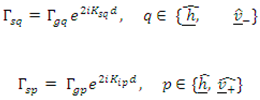
Fresnel reflection coefficients from the ground are given, for the horizontal and vertical fields:
where is the permittivity of ground, and are given as: , , where is the incidence angle.
The study in [3] identified the effects of four paths of the bi-static field in (10-14): direct incidence-direct scattered field, reflected-direct field, direct-reflected field, and reflected-reflected field. The reflection coefficients were utilized solely in terms of their magnitudes; thus, when the absolute value is computed, it will equal unity. It is necessary to determine the horizontal and vertical reflection coefficients. The various types of wavenumbers and the permittivity of the ground are essential for these considerations. The impact of ground on bi-static fields is assessed for two types of grounds, as indicated in references [11,12]. The backscattering coefficients of a vegetation layer over flat ground are provided using a discrete scatterer model. The value ε_g=12+j3 indicates a volumetric water content of 0.3, signifying dry ground conditions. The wavenumber k0 was determined to be 110.23 in prior research, and the incidence angle is 30°. The wavenumbers are derived from this information. The magnitudes of the Fresnel reflection coefficients were computed using horizontal and vertical formulas. The Fresnel reflection coefficients are derived, and utilizing these values while disregarding variations in other parameters in equations (10-14), the influence of the bistatic fields on coherence can be determined. Previously, the coherence of the direct incidence and direct scattered field was examined, excluding Fresnel reflection coefficients. Figure 8 illustrates the coherence between the reflected and direct fields. Compared to Figure 9, the new coherence has decreased due to the Fresnel reflection coefficients Γ_sh for the horizontal component and Γ_sv for the vertical component, as illustrated in Figure 8 and Figure 9.
Moreover, the reflected-reflected field reduces coherence due to the multiplication of the squares of two Fresnel reflection coefficients. This indicates a notable reduction in coherence, as illustrated in Figure 8 for horizontal components and Figure 9 for vertical components. This important issue is also highlighted in [9]. The terms related to ground-volume-ground reflections, which involve two specular reflections, may have been omitted due to their typically small magnitude resulting from attenuation in vegetation.
3.2. Effect of Vegetation Forward Scattering Amplitude on Coherence
The previously, γ is defined as follows:
The extinction coefficient (σ_x) and incidence angle (θ) yield a value of γ equal to 0.462 for the simulations conducted. The value is contingent upon the number density of vegetation scatterers (ρ_N), wave number (k), and the imaginary component of the vegetation forward scattering amplitude (Im). Given that ρ_N is defined as a constant, it was assigned a value of one for the simulations of power, phase, and coherence. Using the same ρ_N and γ, Im is determined to be 1.7548 from equation (30).
The sensitivity analysis of scattering amplitude involves calculating and plotting coherence for various imaginary components. Coarse comparisons for Im values ranging from 0.175 to 1.7548 are illustrated in Figure 10 and Figure 11. Various observations can be made from the figure. Figure 10 indicates that, as the amplitude of the imaginary component ranges from 0.175 to 1.7548, InSAR coherence appears to decline with decreasing imaginary component values. Furthermore, as the component diminishes, saturation occurs beyond the point at which the actual component saturates (exceeding 10m). The forward scattering amplitude influences both the saturation point and the coherence magnitude. The imaginary component ranges from 1.7548 to 2.65 in Figure 11. The saturation point stabilizes at approximately 15 meters of tree height.
3.3. Effect on Power
In Figure 12 and Figure 13, InSAR power is plotted for increasing forward scattering amplitude, utilizing the same parameters as previously mentioned. More compact observations can be conducted for the InSAR power. For imaginary component values ranging from 0.175 to 1.7548, both power and saturation point exhibit a decreasing trend, as illustrated in Figure 12. Power reduction progresses from 1.7548 to 2.55; however, the change in power appears diminished, and the saturation point stabilizes beyond the value of 1.7548, as illustrated in Figure 13.
3.4. Effect on Phase
The impact of the forward scattering amplitude on phase, under identical parameters, is illustrated in Figure 14. The forward scattering amplitude increases from 0.175 to 1.7548, resulting in a corresponding increase in phase. However, beyond 1.7548 (Phreal), the variation in phase is minimal.
4. Conclusions
The utilization of models to identify mathematical relationships is crucial for generalizations. Coherence, phase, correlation, and power are directly associated with the vegetation extinction coefficient, tree height, wavelength, radar altitude, biomass, underlying topography, incident angle, scattering mechanisms, and ground surface dielectric properties. The comparison of this discrete interferometric model with Treuhaft’s model for a layer on a random medium concludes that our model generalizes the empirical Treuhaft’s model. The power increases with tree height, and as forest density rises, the maximum power value also increases, both exhibiting apparent saturation beyond a height of 10 m. Coherence improves as B/r1 increases. As θB increases, both the maximum value and the rate of decline in coherence decrease, indicating a clear saturation effect beyond 10 m of tree height for all angles. Contributions of the reflection coefficient resulting from bi-static fields’ influence on vegetation properties. The direct-reflected, reflected-direct, and reflected-reflected bi-static fields appear to reduce coherence. Two specular reflections lead to a notable decrease in coherence, as confirmed by [9].
The dielectric properties of various ground types influence vegetation parameters. Optimal coherence results are achieved with dry ground. The imaginary component of the forward scattering amplitude influences coherence; however, the relationship does not appear to be proportional. Power yields more compact results regarding alterations in the forward scattering amplitude. As the forward scattering amplitude increases, the power and saturation point decrease. The mathematical relationships concerning coherence, phase, and power provide clear indicators for estimating the outcomes of parameter modifications. Subsequent research should involve validating these simulation results against empirical data obtained from various radar measurements.
Author Contributions
Conceptualization, F.C. and S.SS..; methodology, R.H.L.; software, F.C..; validation, F.C., S.S.S., and R.H.L.; formal analysis, F.C.; investigation, F.C.; resources, F.C.; data curation, S.S.S. and R.H.L; writing—original draft preparation, F.C.; writing—review and editing, F.C.; visualization, S.S.S.; supervision, R.H.L.; project administration, R.H.L. All authors have read and agreed to the published version of the manuscript
Funding
This research received no external funding.
Institutional Review Board Statement
Not applicable.
Acknowledgments
We would like to express our gratitude to Özlem Şimşek and Nil Gürel for their valuable contributions.
Conflicts of Interest
The authors declare no conflicts of interest.
References
- Treuhaft, R.N.; et al. Vegetation characteristics and underlying topography from interferometric radar. Radio Sci. 1996, 31, 1449–1485. [Google Scholar] [CrossRef]
- Treuhaft, R.N.; Siqueira, P.R. The calculated performance of forest structure and biomass estimates from interferometric radar. Waves Random Media 2004, 14, 345. [Google Scholar] [CrossRef]
- Seker, S.S.; Lang, R.H. A discrete interferometric model for a layer of random medium. In Proceedings of the 2009 IEEE International Geoscience and Remote Sensing Symposium, Cape Town, South Africa, 12–17 July 2009; pp. II-674-II-677. [Google Scholar]
- Skolnik, M. Radar Handbook, 3rd ed.; Mc Graw Hill: New York, NY, USA, 2008; pp. 1.2–1.10. [Google Scholar]
- Zebker, H.A.; Goldstein, R.M. Topographic mapping from interferometric synthetic aperture radar observations. In: NASA (JPL Aircraft SAR Workshop Proc. 1985.
- Rodriguez, E.; Martin, J.M. Theory and design of interferometric synthetic aperture radars. IEE Proc. F (Radar Signal Process.) 1992, 139, 147–159. [Google Scholar] [CrossRef]
- Hagberg, J.O.; Ulander, L.M.H.; Askne, J. Repeat-pass SAR interferometry over forested terrain. IEEE Trans. Geosci. Remote Sens. 1995, 33, 331–340. [Google Scholar] [CrossRef]
- Treuhaft, R.N.; Cloude, S.R. The structure of oriented vegetation from polarimetric interferometry. IEEE Trans. Geosci. Remote Sens. 1999, 37, 2620–2624. [Google Scholar] [CrossRef]
- Treuhaft, R.N.; Siqueira, P.R. Vertical structure of vegetated land surfaces from interferometric and polarimetric radar. Radio Sci. 2000, 35, 141–177. [Google Scholar] [CrossRef]
- Sarabandi, K.; Lin, Y.C. Simulation of interferometric SAR response for characterizing the scattering phase center statistics of forest canopies. IEEE Trans. Geosci. Remote Sens. 2000, 38, 115–125. [Google Scholar] [CrossRef]
- Seker, S.S. EM propagation and backscattering discrete model for the medium of sparsely distributed lossy random particles. AEU-Int. J. Electron. Commun. 2007, 61, 377–387. [Google Scholar] [CrossRef]
- Seker, S.S. Microwave backscattering from a layer of randomly oriented discs with application to scattering from vegetation. In: IEE Proceedings H (Microwaves, Antennas and Propagation). IET Digital Library 1986, 497–502. [Google Scholar]
Figure 1.
Representation of the real and imaginary parts of the InSAR cross-correlation, for only two vegetation altitudes.
Figure 1.
Representation of the real and imaginary parts of the InSAR cross-correlation, for only two vegetation altitudes.
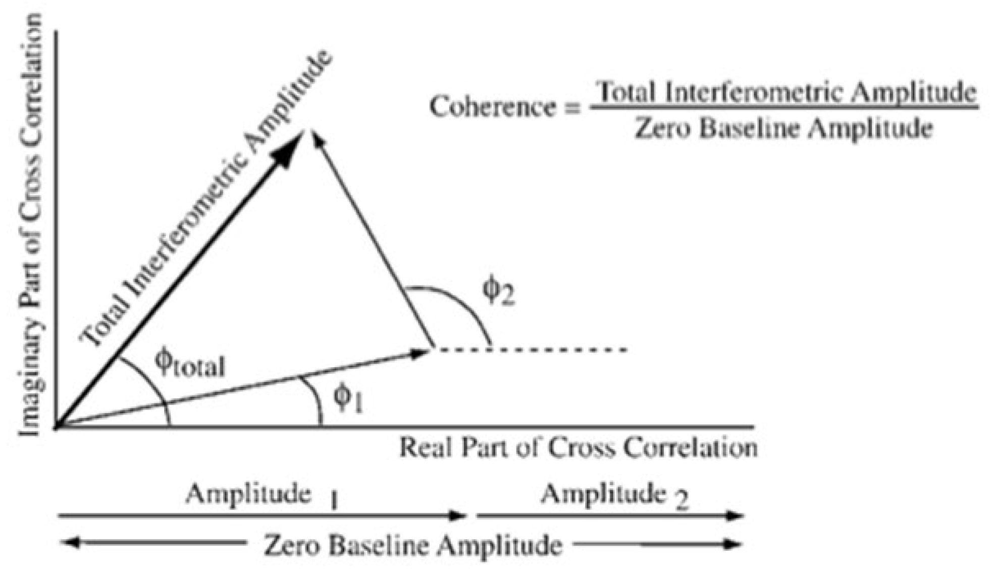
Figure 2.
The InSAR figure, with a horizontal baseline B and horizontal ground surface.
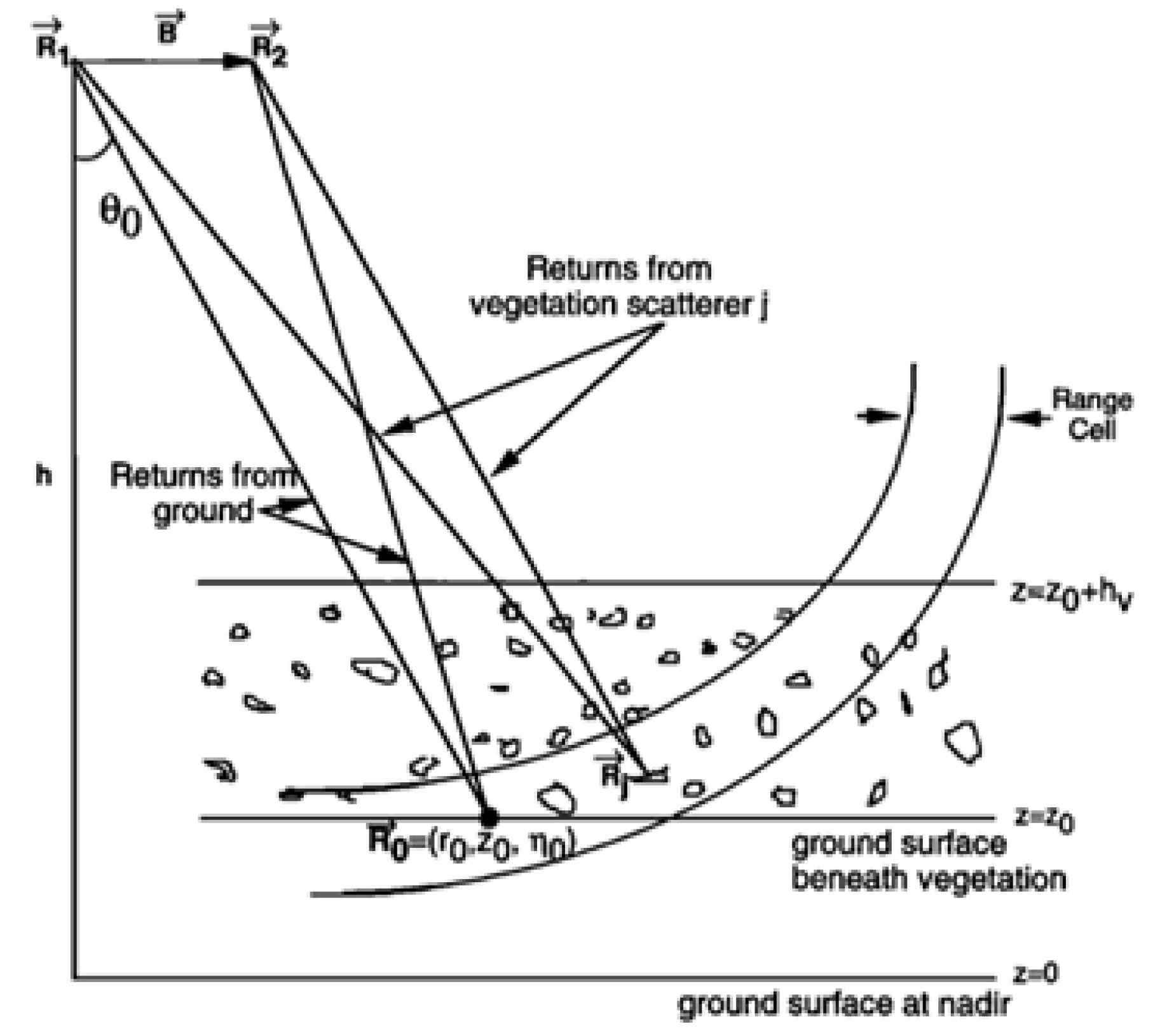
Figure 3.
Random layer of a medium.
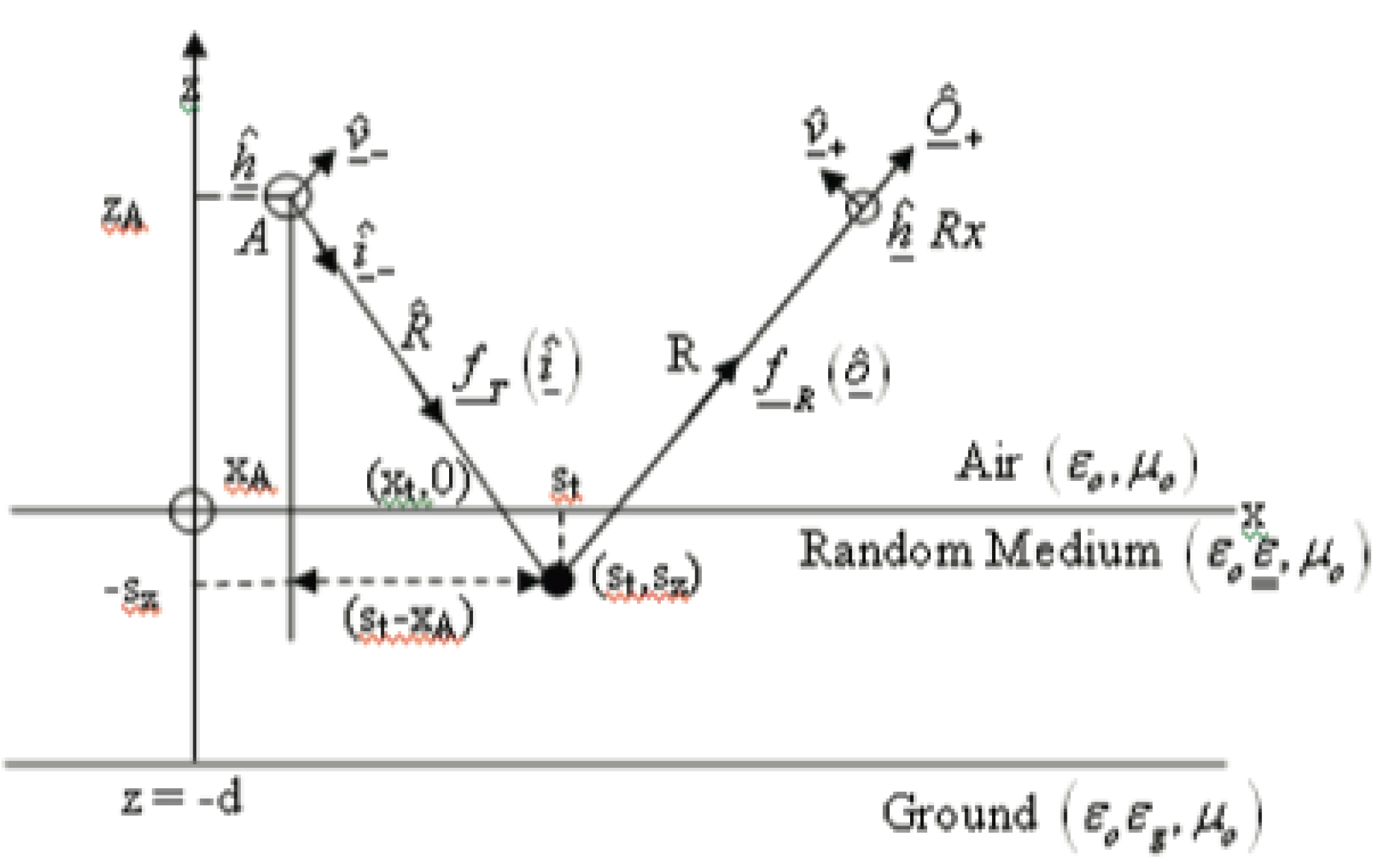
Figure 4.
The four paths of the bi-static field. (a) Direct Incidence - Direct Scattered Field; (b) Reflected – Direct Field; (c) Direct – Reflected Field; (d) Reflected – Reflected Field [11,12].
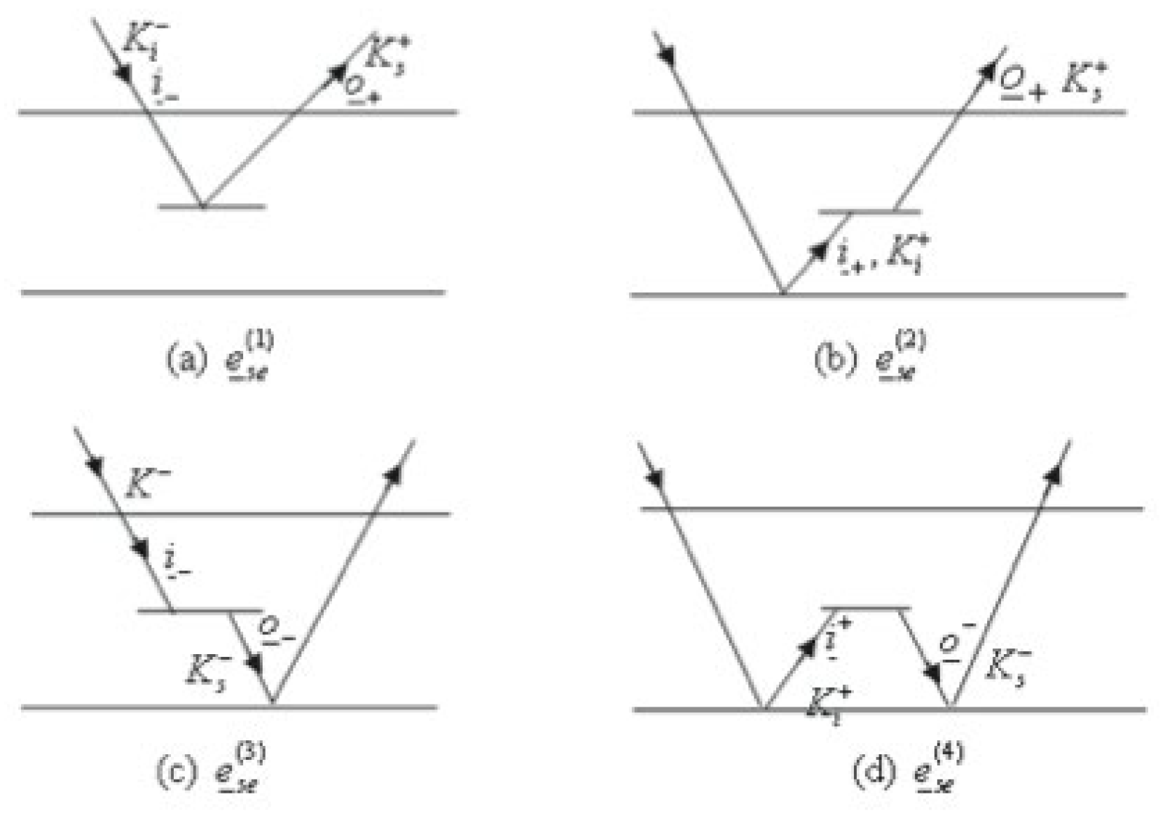
Figure 5.
Power in terms of tree height with changing forest density.
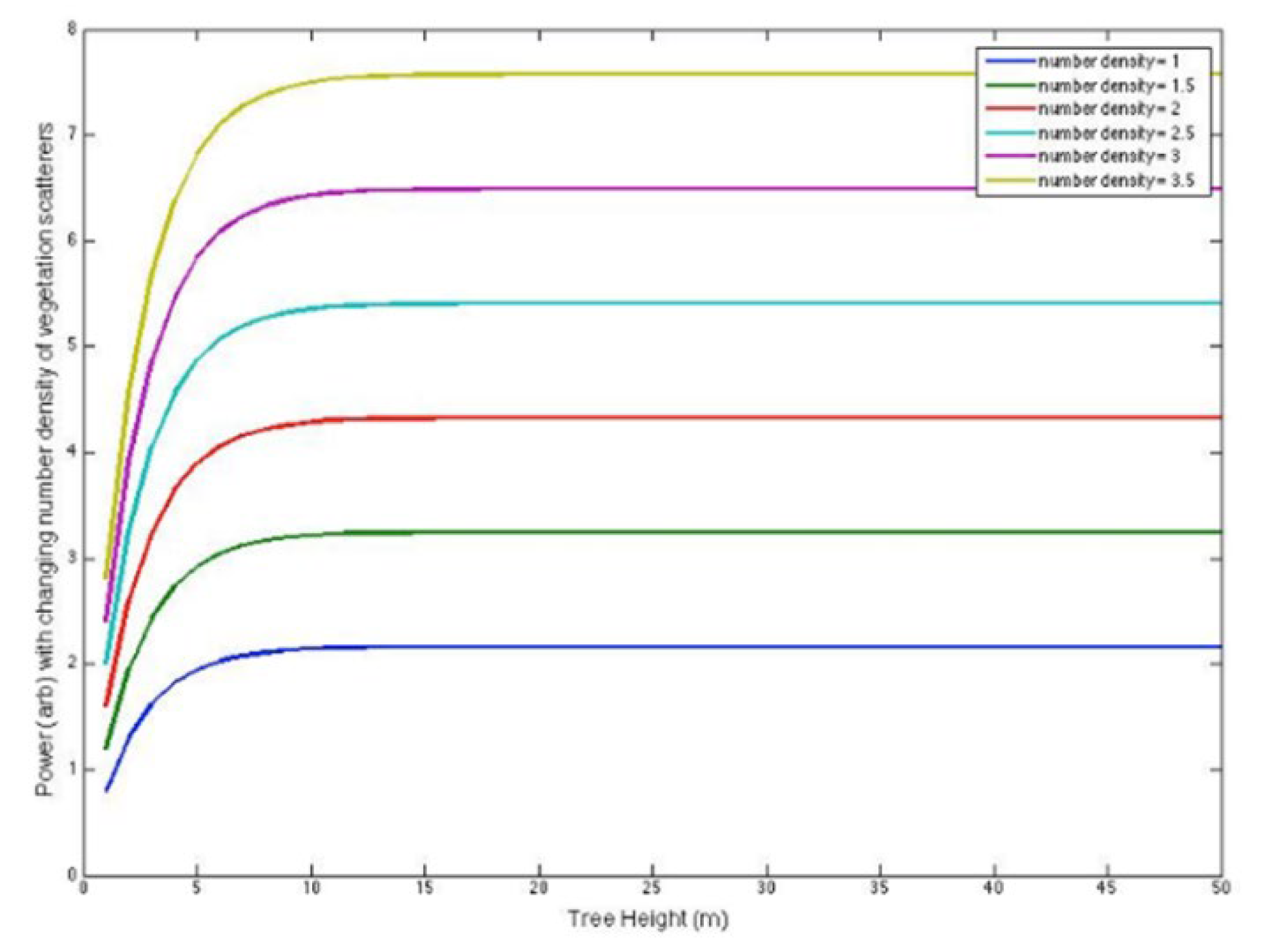
Figure 6.
InSAR coherence in terms of tree height concerning changing θB.
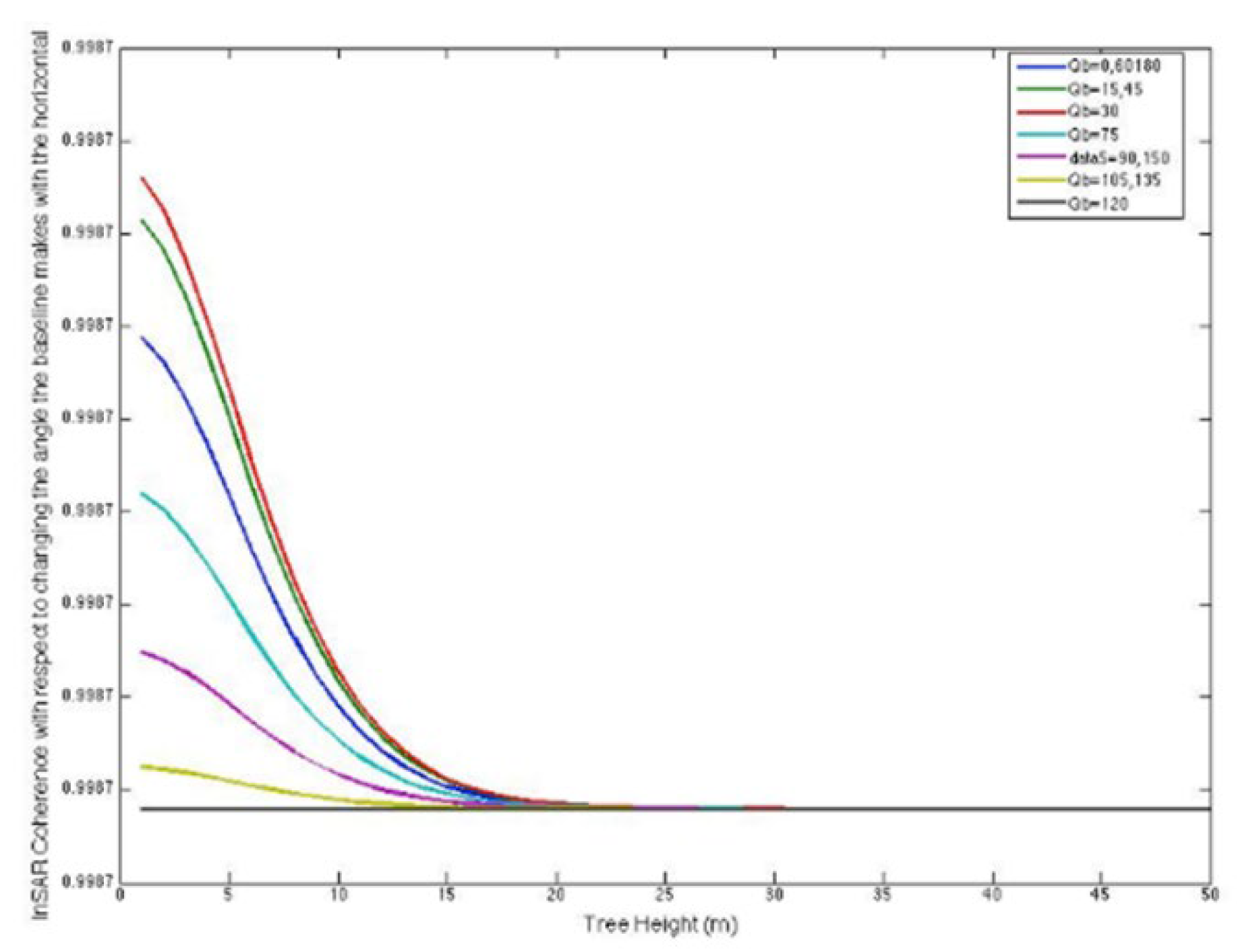
Figure 7.
InSAR coherence in terms of tree height with slightly changing B/r1 ratio.
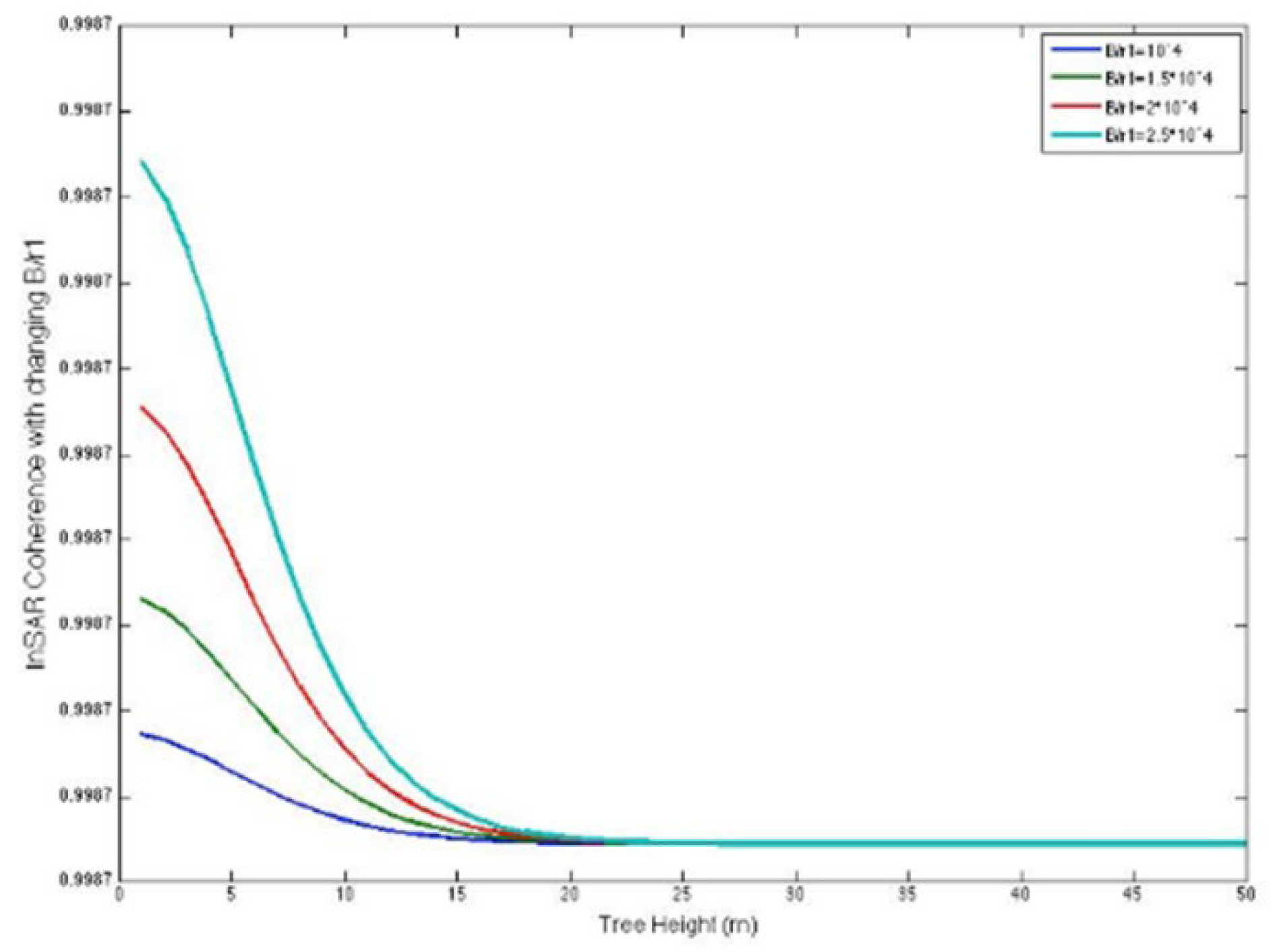
Figure 8.
Horizontal component of the reflected – direct bi-static field effect on coherence vs. function of tree height for ε_g=12+j3.
Figure 8.
Horizontal component of the reflected – direct bi-static field effect on coherence vs. function of tree height for ε_g=12+j3.
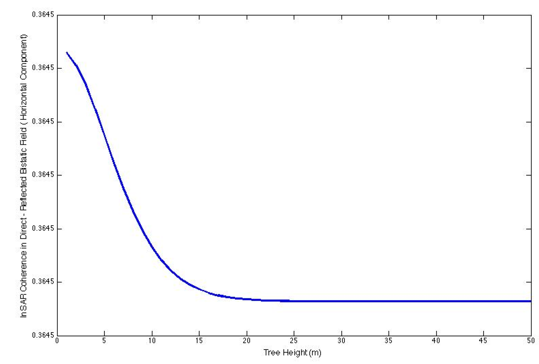
Figure 9.
Vertical component of the reflected–direct bi-static field effect on coherence vs. tree height for ε_g=12+j3.
Figure 9.
Vertical component of the reflected–direct bi-static field effect on coherence vs. tree height for ε_g=12+j3.
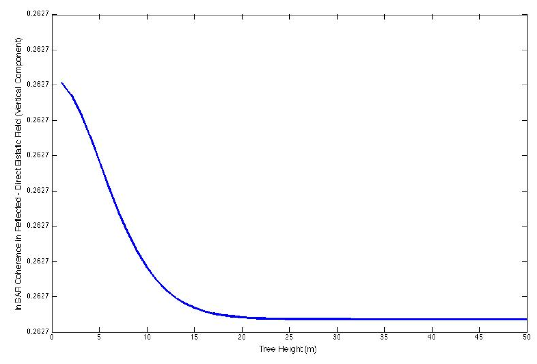
Figure 10.
Forward scattering smplitude effect on coherence.
Figure 11.
Forward scattering amplitude effect on coherence.
Figure 12.
Forward scattering amplitude effect on power.
Figure 13.
Forward scattering amplitude effect on power.
Figure 14.
Forward scattering amplitude effect on phase.
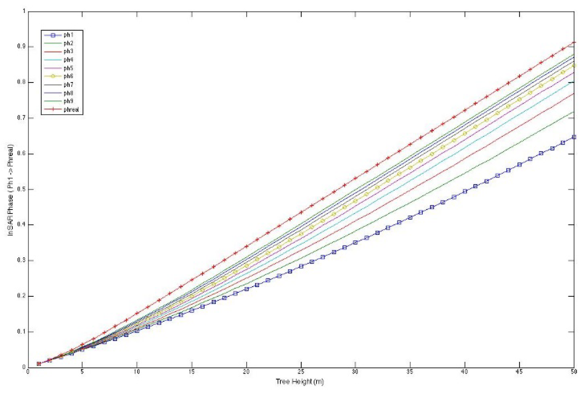

Table 1.
The terms used in the models.
| Term in Treuhaft Model | The Corresponding Term in the Seker Model |
|---|---|
| sz | |
| Bistatic Fields in [3] | Corresponding Scattering Mechanisms in [2,9] |
|---|---|
| Direct Incidence-Direct Scattered Field | Direct Ground |
| Reflected-Direct Field | Specular Ground-Volume |
| Direct-Reflected Field | Specular Volume-Ground |
Table 3.
Parameters used in simulations.
| Parameter | Value |
|---|---|
| Extinction Coefficient (σx) | 0.2 db/m |
| Baseline Distance | 5 m |
| Incidence Angle (θ) | 30° |
| Wavelength (λ) | 5.7 cm (C-Band) |
| Radar Altitude | 8 km |
| B/r1 | 10-4 |
Table 4.
Parameters used in simulations.
| θ: Incidence Angle | σx: Extinction Coefficient | γ | k: Wavenumber | B/r1 | αz: vettical Wavenumber |
|---|---|---|---|---|---|
| 300 | 0.2 db/m | 0.462 | 110.23 | 10-4 | 1.909*10-2 |
Disclaimer/Publisher’s Note: The statements, opinions and data contained in all publications are solely those of the individual author(s) and contributor(s) and not of MDPI and/or the editor(s). MDPI and/or the editor(s) disclaim responsibility for any injury to people or property resulting from any ideas, methods, instructions or products referred to in the content. |
© 2025 by the authors. Licensee MDPI, Basel, Switzerland. This article is an open access article distributed under the terms and conditions of the Creative Commons Attribution (CC BY) license (https://creativecommons.org/licenses/by/4.0/).
Copyright: This open access article is published under a Creative Commons CC BY 4.0 license, which permit the free download, distribution, and reuse, provided that the author and preprint are cited in any reuse.


