Establishing Models for Predicting Above Ground Carbon Stock Based on Sentinel 2 Imagery for Evergreen Broadleaf Forests in South Central Coastal Ecoregion, Vietnam

1. Introduction

Many vegetation indices play a critical role in estimating biomass and monitoring plant growth, yet each index employs a distinct approach and has certain limitations. Soil Adjusted Vegetation Index (SAVI) was developed to mitigate the influence of soil conditions, thereby enhancing accuracy in areas with sparse vegetation, though it is less effective in regions with dense vegetation [1]. Chlorophyll Vegetation Index (CVI) measures chlorophyll concentration and is highly useful for assessing plant health and development; however, it may be limited in areas with low chlorophyll levels [2]. Green Leaf Index (GLI) reflects the greenness of leaves and is particularly accurate during periods of rapid growth, but its effectiveness diminishes in areas with dense vegetation cover [3]. Normalized Difference Vegetation Index (NDVI) stands out for its stability when applied on a large scale and its suitability for regions with abundant vegetation. It is calculated based on the difference between near-infrared and red light reflectance, which helps measure the level of photosynthetic activity and vegetation growth, thereby effectively estimating biomass and stored carbon [4]. Furthermore, NDVI provides precise information regarding vegetation density and health, key factors in assessing carbon stocks [5]. Additionally, NDVI has stability over time, making it particularly advantageous for use in areas with dense and abundant vegetation, thus facilitating effective large-scale assessments [6]. Therefore, some previous studies have developed regression equations for estimating above ground biomass (AGB) of natural forests based on vegetation indices from Landsat, Sentinel imageries, such as NDVI, EVI, SAVI [7,8,9,10].

Currently, estimation of forest carbon stock and flows have applied by various methods, from the simple forest biomass inventory to complex, sophisticated experiments and models, which are forest inventory, remote sensing, eddy covariance and the inverse method [11]. Among these methods, remote sensing technology has become the main tool to overcome some limitations of ground data collection from filed sample plots in forest monitoring and inventory at a landscape scale by improving accuracy and reducing costs [12,13,14]. It also has considered as the cheapest method if there are suitable resolution and spatial scale since the developing countries with limited capacities in collecting and managing data need to apply the low cost methodologies but spatial and temporal resolutions are acceptable and ratio of sample plots are appropriative [11]. Therefore, over the past decade, Sentinel-2 satellite data has been widely applied for estimating the biomass of natural forests due to its high resolution. Investigating the relationship between Sentinel-2 image indices (NDVI, EVI, NDI45, etc.) and above-ground biomass (AGB) in privately managed tropical forests in Indonesia found that the NDI45 exhibited strong correlation with AGB in comparison to other indices (r = 0.89; R² = 0.79) [10]. Moreover, Sentinel-2 imagery has been integrated with EnMAP to map and monitor environmental changes [8] or with PlanetScope to develop biomass mapping models [15]. Estimating biomass and carbon accumulation capacity of tropical rainforest in Kon Ha Nung plateau based on EVI index of Sentinel-2 images, Dang, H.N. et al. demonstrated that lin-log models established to estimate biomass from EVI index of Sentinel-2 images in 2016 and 2021 both had the highest R² value, 0.76 and 0.765, respectively [8].

In Vietnam, the UN-REDD (Reducing Emissions from Deforestation and forest Degradation) program has developed allometric equations for each forest type in each ecological region and a generic equation for a nation by using the destructive method to estimate biomass and carbon stocks [16]. However, the destructive method is both time-consuming and costly, making it impractical for application in large, inaccessible forest areas [17]. Although the relationship between remote sensing indices and forest inventory factors has been determined, biomass is a decisive condition for the effectiveness of remote sensing in forest resource monitoring. However, it appears that very few studies have examined the correlation between biomass, carbon stocks, and remote sensing indices for monitoring forest carbon at national, regional, or global scales [18]. Meanwhile, the Sentinel 2 image has quite high resolution and suitable for analyzing the relationship of forest vegetation reflectance indices with forest biomass, furthermore the Sentinel 2 images are free of charge so it contributes to reducing costs in estimating natural forest carbon stocks. In this context, this study was conducted with aim to develop correlation equations between natural forest carbon stocks and indices of Sentinel 2 images through linear and non-linear models to directly estimate stored carbon for assessing carbon emission and removal in the South Central Coastal Ecoregion, Vietnam.

2. Materials and Methods

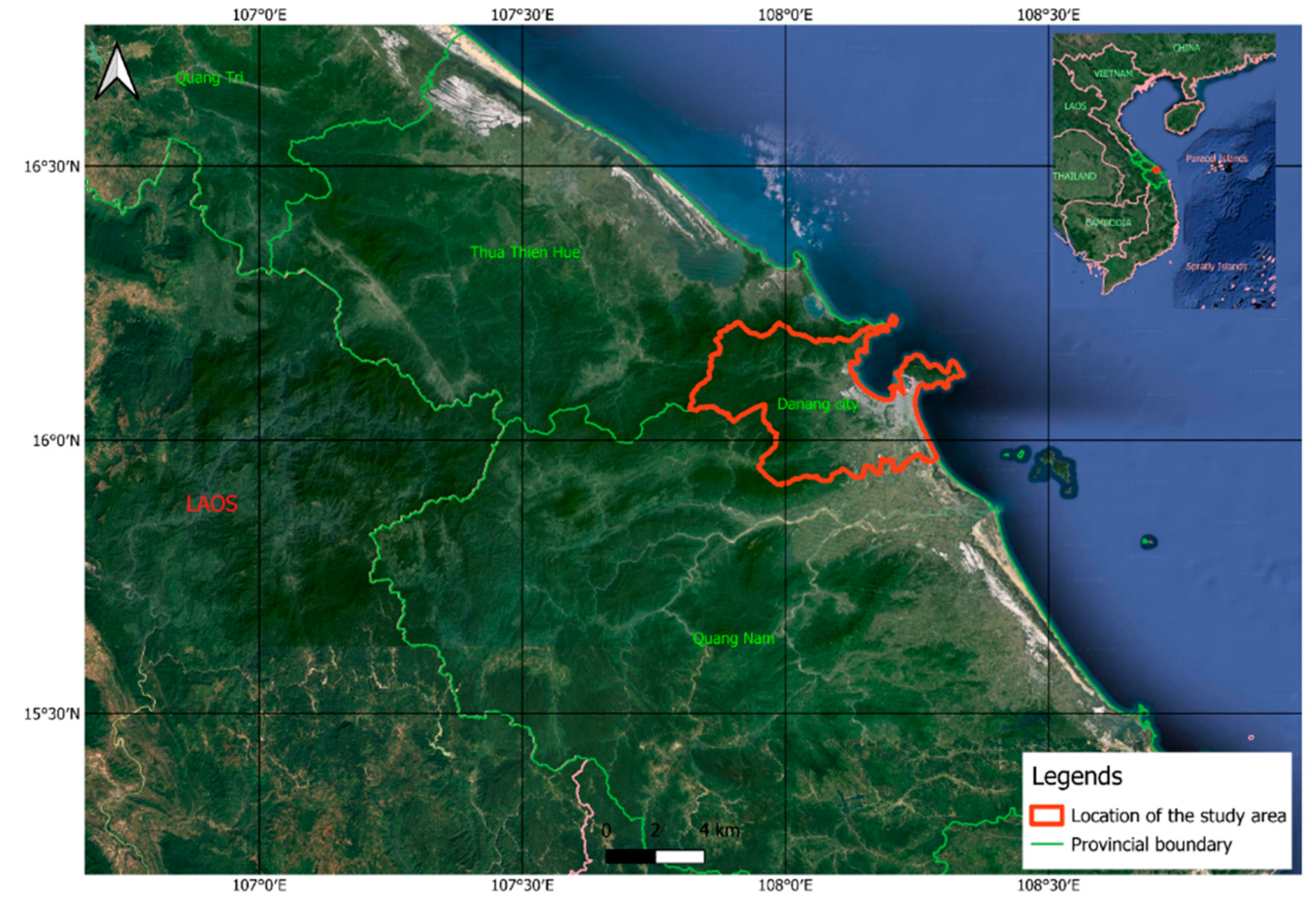
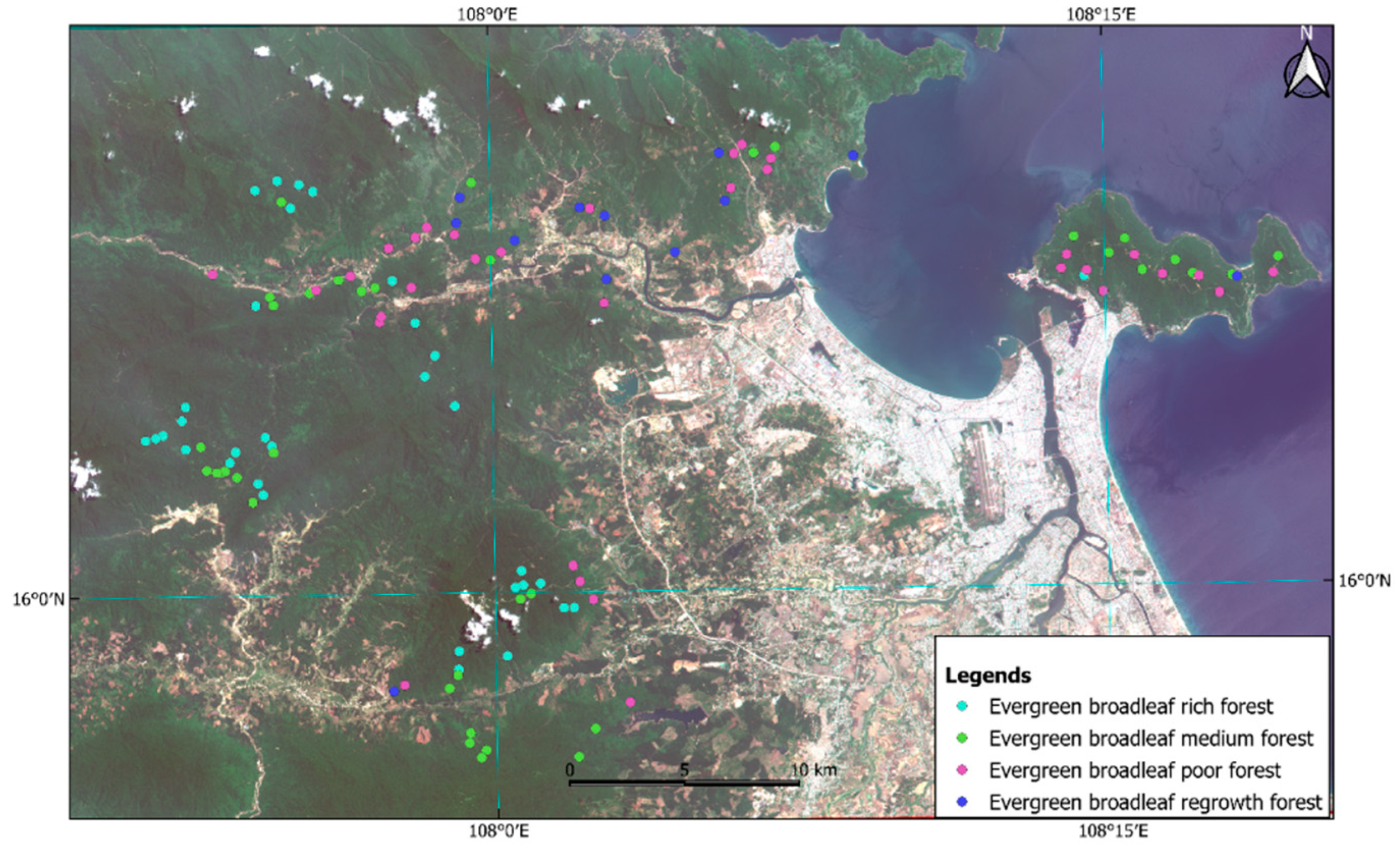
2.1. Study Area

This study was conducted in Da Nang city that belongs to South Central Coastal (SCC) ecoregion of Viet Nam (Figure 1), is one of eight agricultural ecoregion divided following climate, altitude and soil conditions [19,20]. Da Nang city is located in a typical monsoon climate zone with two distinct seasons: dry season from January to August and rainy season from September to December. Average annual temperature is 25.8⁰C, average annual precipitation is 2,153 mm, and average humidity is 83.4%. Its terrain has both coastal delta and mountains, in which the mountainous area has evaluation of 700-1,500 m and slopes over 40⁰ with the watershed forests occupies a large area [21]. Natural forest in Da Nang city is Evergreen Broadleaf Forest (EBF) type with total of 43,061.90 hectares [22], including four forest types: rich forest, medium forest, poor forest, and regrowth forest.

2.2. Sample Plots and Estimation of Total Above Ground Carbon

Total 115 sample plots of 1,000 m² (40 m x 25 m) were established that are representative of four forest classes, which are 33 sample plots representative of rich forest, 37 sample plots representative of medium forest, 33 sample plots representative of poor forest, and 12 sample plots representative of regrowth forest (Figure 2). All standing trees with DBH ≥ 6cm within sample plots were defined species name (both local and scientific names) and were measured DBH (cm), H (m), meanwhile WD were derived from the data that used for establishing biomass equations for EBF in South Central Coastal Ecoregion of Viet Nam [23] or from the ICRAF’s WD data (http://db.worldagroforestry.org/wd) in case of these trees are outside of above species.

For this study, AGB of individual tree was estimated by applying the AGB equation developed by Huy et al (2016) for EBF in SCC ecoregion of Vietnam. Due to the equation with combination of two covariates (DHB²H) and of three covariates (DHB²HWD) are more appropriate than with single variable [23], this study, therefore was applied the equation below for estimating AGB

AGB = 0.598313 x (DBH² x HWD)^0.959790

(1)

Where: AGB is expressed in kg; DBH is expressed in centimeters cm; H is expressed in m; WD is expressed in g/cm³; and 0.598313 and 0.959790 are constants.

Total above ground biomass (TAGB) of sample plot was calculated from AGB of individual tree, then converted to per hectare (Mgha^-1). The TAGC was converted from TAGB by using the carbon fraction (CF) of IPCC (2006), specific equation for calculating TAGC is [24]:

TAGC = TAGB x 0.47

(2)

Where: TAGC is expressed in Mgha-1; TAGB is expressed in Mgha-1; and 0.47 is default value for CF.

2.3. Sentinel-2 Image and Identification of Key Indices

In Da Nang city, the dry season extends from January to August each year; therefore, remote sensing images taken during this season should be selected as they will be less affected by clouds, ensuring accuracy in the image interpretation process. This study used Sentinel-2 images with a panchromatic resolution of 10 m × 10 m and a multispectral resolution of 20 m × 20 m to interpret and calculate vegetation indices (VIs) based on four typical multispectral bands: BLUE, GREEN, RED, and NIR. The scene “S2B_MSIL1C_20230522T030529_N0509_R075,” captured on May 22, 2024 and downloaded from https://scihub.copernicus.eu/, was interpreted and calculated VIs related to vegetation covers.

Using VIs obtained from remote sensing analysis of foliage to quantify and qualitatively assess vegetation cover, vitality and growth is a fairly simple and effective method. However, different VIs reflect different vegetation, so each VI is often suitable for a few specific uses under certain conditions [25]. Therefore, this study has identified 5 VIs closely related to forest vegetation to establish a TAGC estimation model (Table 1)

2.4. Development of Regression Models

The VIs and multispectral bands that have a significant influence on TAGC prediction were identified using Principal Component Analysis (PCA). Total 10 variables were conducted through PCA with package ‘ggplot2’, ‘factoextra’, ‘dplyr’, ‘ggfortify’, ‘pracma’ [29]. In which, TAGC that was calculated from 115 sample plots, and 5 VIs (ARVI, EVI, NDVI, SAVI, SIPI) and 4 multispectral bands (BLUE, GREEN, RED, NIR) that were identified from Sentinel-2 image “S2B_MSIL1C_20230522T030529_N0509_R075”. Based on the PCA results, the first two principal components (PC) are selected to identify the VIs and multispectral bands that have a significant influence on TAGC if the overall variability of the dataset reaches 80% or more; if not, additional PCs will be included until this threshold is met, since PCA provides an approximation of the original dataset by using some PCs [30]

PC1 is used to determine the weight of each variable, and this is combined with the component weight relationship graph between PC1 and PC2 to select those VIs and multispectral bands with high absolute weight values and a significant influence on TAGC. Based on these findings, the linear and non-linear with weight models (both single variable and variable combination) will be determined. In addition to applying powers models as many previous studies have applied to establish correlation equations to estimate AGB based on forest inventory factors such as DHB, H, WD, etc. [23] or based on VIs [7,8,9,10], exponential and quadratic models are also established to select the fit models.

2.5. Cross Validation

Correlation models were established and validated for model comparison and selection using Monte Carlo cross-validation method [23,31,32]. The dataset was randomly divided into two parts for each iteration, in which 80% of the sample was used for model establishment and the remaining 20% was used for model validation. The cross-validation process was repeated 100 times, the statistics and errors of the model were averaged for 100 iterations.

Linear models were constructed and cross validated using the ordinary least squares method with the ‘lm’ package [29]. The weighting scheme was defined as W = 1/X^α, where X represents the vegetation indices (VIs) and multispectral bands that significantly influence TAGC, and α = ±2 [33]. Non-linear models were developed and cross validated using the Maximum Likelihood method via the ‘nlme’ package [29,31], with the weighting scheme defined as W = 1/X^δ, where δ is the variance function coefficient [23,31,32,34].

The Akaike Information Criterion (AIC) developed by [35] and applied by Huy et al. [23,31,32,34] was used to validate, compare and select fit models. In addition, the R² and the main errors such as Average Systematic Error (ASE), Root Mean Square Error (RMSE), and Mean Percent Standard Error (MPSE) [23,31,36] are also used along with the AIC for model selection. AIC, R², ASE, RMSE, and MPSE are calculated from 20% of the dataset used to validate the model for each iteration and are averaged over 100 iterations.

$$R^2={\displaystyle \frac{1}{R}}{\sum }_1^R\left(1-{\displaystyle \frac{\sum _{j=1}^m{\left(Y_j-\widehat{Y_j}\right)}^2}{\sum _{j=1}^k{{(Y}_j-\overline{Y})}^2}}\right)$$

(3)

$$ASE(\%)={\displaystyle \frac{1}{R}}{\sum }_1^R{\displaystyle \frac{100}{m}}\sum _{j=1}^m{\displaystyle \frac{Y_j-{\widehat{Y}}_j}{{\widehat{Y}}_j}}$$

(4)

$$RMSE\left(Mg{ha}^{-1}\right)={\displaystyle \frac{1}{R}}{\sum }_1^R\sqrt{{\displaystyle \frac{1}{m}}\sum _{j=1}^m{{(Y}_j-{\widehat{Y}}_j)}^2}$$

(5)

$$MPSE(\%)={\displaystyle \frac{1}{R}}{\sum }_1^R{\displaystyle \frac{100}{m}}\sum _{j=1}^m\left|\left.{\displaystyle \frac{Y_j-{\widehat{Y}}_j}{{\widehat{Y}}_j}}\right|\right.$$

(6)

Where R is the number of iterations (100) in cross-validation; m is the number of sample plots in the validation dataset (20% of randomly selected data); and Y_j, ${\widehat{Y}}_j$ $\mathrm{a}\mathrm{n}\mathrm{d}\overline{Y}$represent the TAGC (Mg ha^-1) of the observed, predicted, and mean values, respectively, for the j-th sample plot during the R iterations of cross-validation.

The selected models are those with the best indices (i.e., the lowest AIC, the highest R², and the smallest errors in ASE, RMSE, and MPSE). However, in practice, it is very challenging for a model to optimize all five indices simultaneously. Therefore, models with an AIC lower than the average AIC of all models and an R² greater than 0.85 (with higher values being preferable) are chosen for further parameter identification and validation.

The statistical software R [29] is employed using 100% of the data and 100 iterations to determine and verify the existence of the model parameters. Models that exist all parameters (with p-value < 0.05) and have an MPSE of less than 30% are considered acceptable.

3. Results

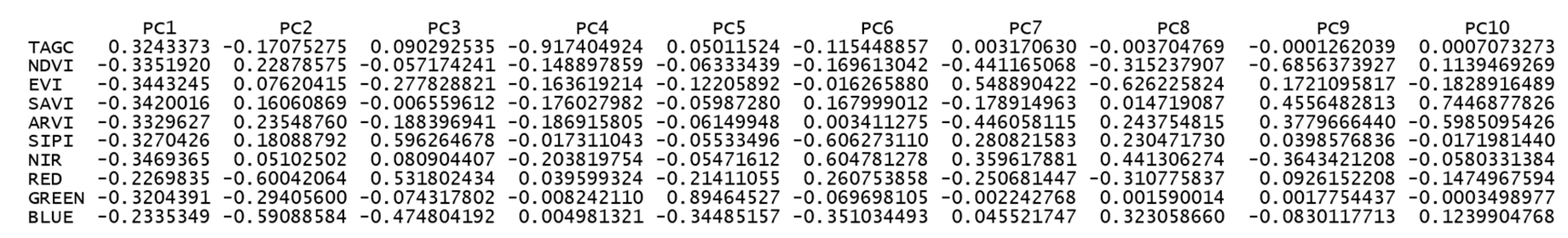
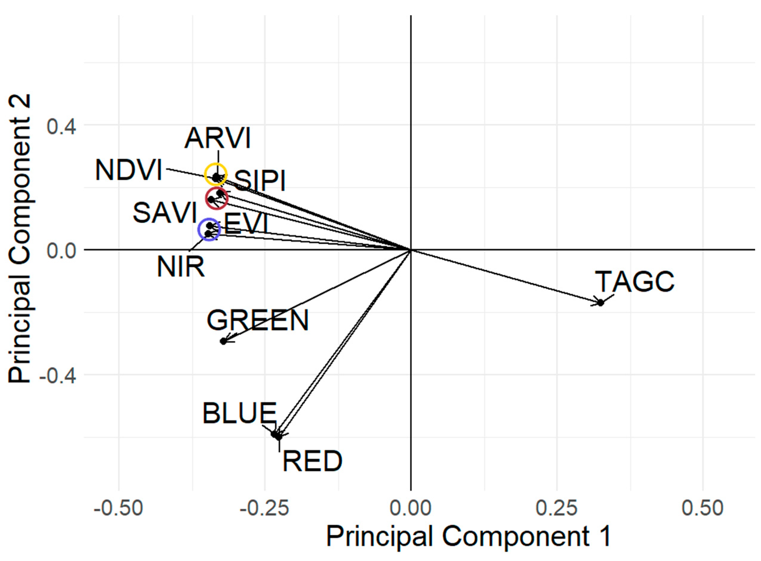
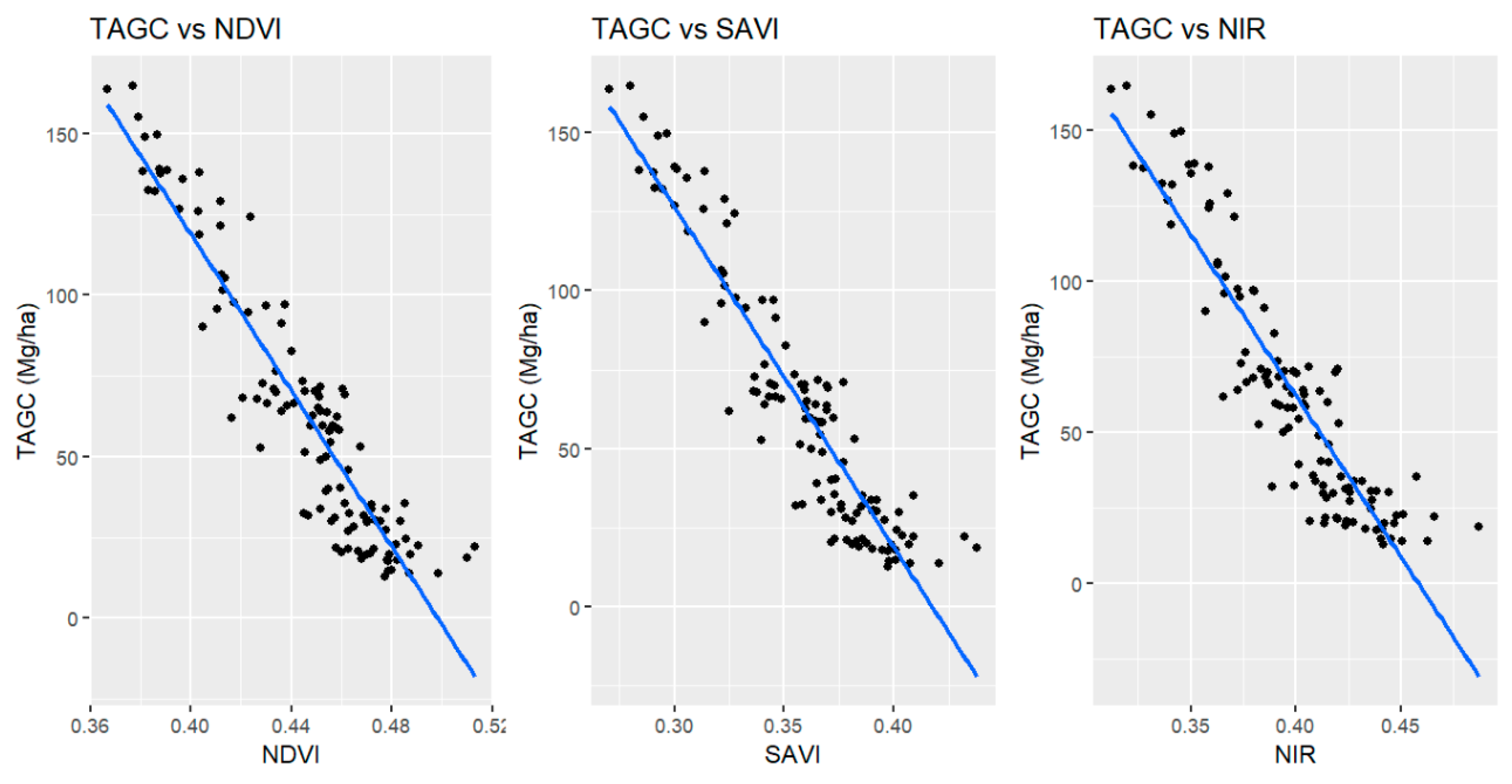
3.1. Vegetation Indices and Multispectral Bands Influencing on Above Ground Carbon

From the PCA results of 10 variables from the data of 115 sample plots (Figure 3), the first two PCs were selected to analyze and determine the VIs and multispectral bands that have a large influence on TAGC to establish correlation models, because these two PCs account for 96.35% of the variation of the original dataset.

Since PC1 accounts for the largest share of variance in the original dataset (82%), it was used to determine the weight of each of the 10 variables (Figure 4) and to analyze the relationship matrix of these variables in the context of the correlation between PC1 and PC2 (Figure 5).

The equation indicating weight of variables following PC1 is presented as follows:

PC1 = 0.3243373 x TAGC - 0.3351920 x NDVI - 0.3443245 x EVI - 0.3420016 x SAVI -0.3329627 x ARVI - 0.3270426 x SIPI - 0.3469365 x NIR - 0.2269835 x RED - 0.3204391 x GREEN - 0.2335349 x BLUE.

(2)

The variables BLUE, RED and GREEN have small weights and are separate, with unclear effects on TAGC (Figure 5), so these variables are excluded from establishing correlation models. TAGC has a close and inverse relationship with the variables NAVI, EVI, SAVI, ARVI, SIPI, NIR; and these variables have a close relationship with each other in pairs, so they form variable groups in the regression model with TAGC, which are the groups (NAVI, ARVI), (SAVI, SIPI), (NIR, EVI), respectively represented in the yellow, red, and blue circles in Figure 5. In addition, in each of the above variable combinations, the variables NAVI, SAVI, NIR have higher weights than the remaining variable (Figure 4), so they are also selected to establish a regression model with TAGC in single variable form.

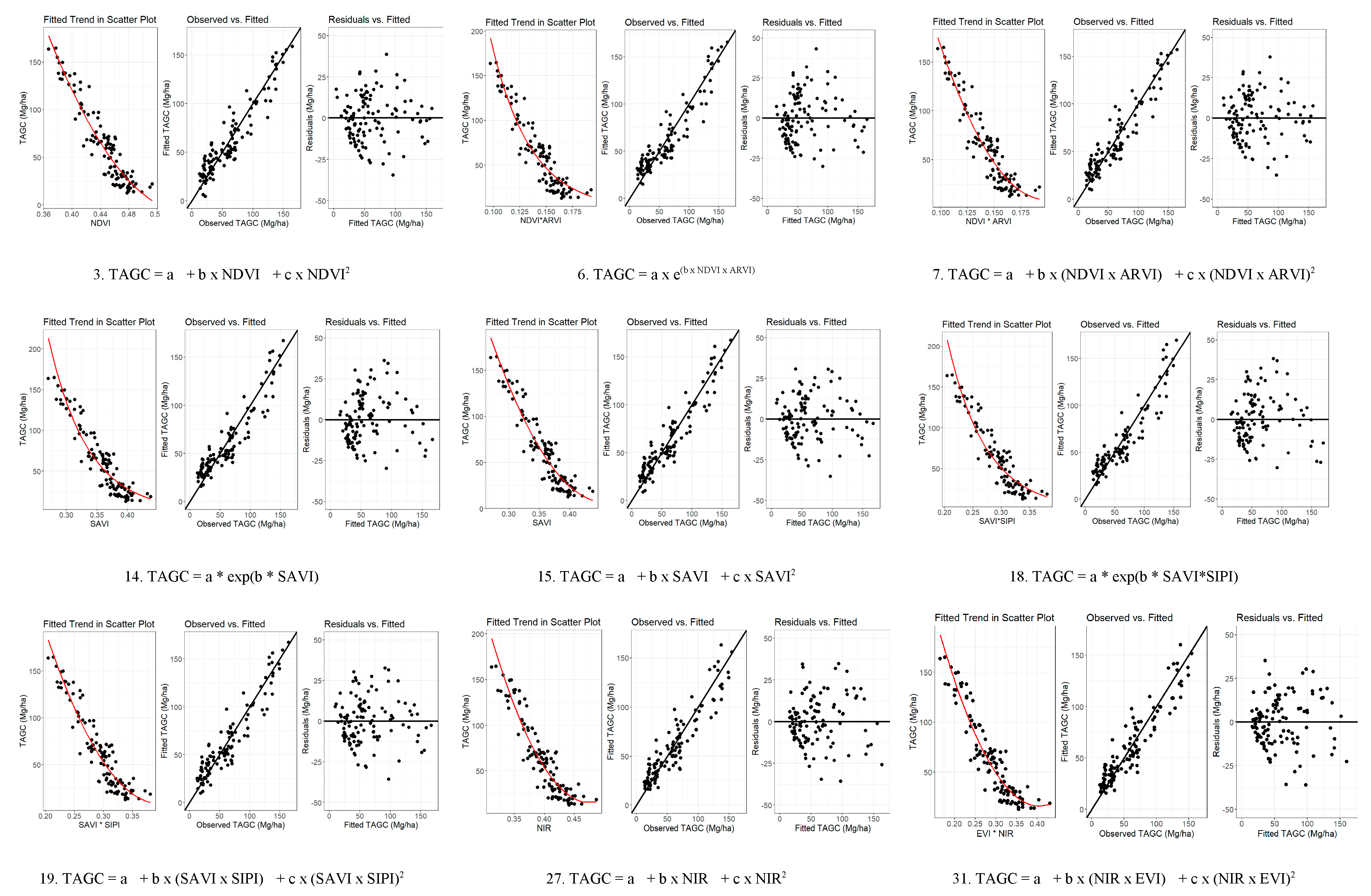
3.2. Establishment of Above Ground Carbon Estimation Models

The PCA results selected three single variables and three variable combinations that have a significant influence on TAGC. An analysis of TAGC variations with respect to NDVI, SAVI, and NIR showed that TAGC differentiates strongly when these variables are small (Figure 6). Consequently, it is necessary to develop models of single variable or variable combination with weight to improve the differentiation of the model’s predicted values (Table 2).

From the equations presented in Table 2, 36 equations were establish and compared for selecting fit models. The regression equations were established with an average AIC value of 766.691 (the smallest value was 748.717, the largest value was 785.717) and R² values ​​ranging from 76.3% to 89.1%. Among these, 16 regression equations with an AIC < 766.691 (ranging from 748.983 to 765.790) and R² > 0.85 were chosen for estimating and testing the existence of parameters, including 2 linear equations of single variable, 1 linear equation of variable combination, 3 non-linear equations of single variable, and 10 non-linear equations of variable combination (Table 3).

3.3. Determination of Above Ground Carbon Estimation Models

The fit models were estimated and tested for the existence of parameters with data of 115 samples (100% of the dataset). Among the 16 selected fit models, 9 models have parameters with p-value < 0.001 and MPSE values ranging from 21.63% to 26.32% (lower than 30%), including one single variable exponential model (Equation 14), two exponential models of variable combination (Equations 6 and 18), three single variable quadratic models (Equations 3, 15, and 27), and three quadratic models of variable combination (Equations 7, 19, and 31) (Table 4).

Among the 9 models identified as fit models, the quadratic models showed the best AIC, R², and MPSE values. In particular, the variable combination model (NIR, EVI) (Equation 31) and the single variable NIR model (Equation 27) had the best MPSE (lowest) and equivalent, at 21.63% and 22.04% respectively (Table 4). In addition, these two models have fitted trend in the middle of the data cloud (left) or closely follow the observed value on the diagonal (middle) and the residuals (right) have a narrow distribution, and are all according to the fitted values ​​(Figure 7). From these results, two mentioned-above models determined as optimal equations, in which, one equation is representative of single variable quadratic model (TAGC = a + b x NIR + c x NIR²) and one is representative of quadratic model with variable combination (TAGC = a + b x (NIR x EVI) + c x (NIR x EVI)²).

4. Discussion

4.1. Determination of Indices of Sentinel 2 Imagery Influencing TAGC Prediction

Many studies have shown that satellite images are commonly used to build biomass estimation models through their VIs, but most only determine the correlation between AGB and each individual VI [7,8,9,10], [37,38]). Meanwhile, VIs are determined from the multispectral bands BLUE, GREEN, RED, NIR [25], so there is a complex relationship between TAGC, VIs and multispectral bands. Consequently, it is necessary to identify multiple VIs and multispectral bands that are strongly associated with TAGC in order to develop regression equations with sing variable form or variable combination form.

From the PCA results, it was determined that NDVI, SAVI, and NIR have a great influence on TAGC. This result is similar to the study of Poudel et al. (2023), reporting that among the 12 VIs of Sentinel 2 images, NDVI and SAVI are the 2 VIs that have the closest relationship with AGB in both linear and quadratic models [38]. Unlike previous studies, which often only used single indices to establish models, this study identified additionally 3 variable combinations (NDVI, ARVI), (SAVI, SIPI), (NIR, EVI) that have a great influence on TAGC. This limits the loss of information in the original dataset, because PCA reduces the multidimensionality of large datasets, increases the ability to interpret/explain, and minimizes the loss of information in the dataset [39].

As PCA results of previous studies such as PCA results of the Dalat pine’s diameter growth and 4 ecological environmental factors with 66.85%, and 9 climate factors with 77.90% [31], this study conducted PCA with assumption using the first two PCs if they account for 80% total variability in the original dataset. With this assumption, VIs and multispectral band were determined for TAGC prediction with high reliability, since cumulative variance proportion of first two PCs account for 96.35% of total variability in the original dataset (Figure 3)

4.2. Establishment and Validation of Models for Predicting TAGC

Most publications related to the relationship model between AGB and Sentinel 2 image indices (ARVI, EVI, NDVI, SAVI, SIPI) are set up in a linear form without weight, so R² only reaches from 0.57 to 0.75 [38], NDVI of Landsat 8 image only gives R² = 0.43 [40] or linearized log-log, log-lin function with EVI gives R² = 0.60-0.76 [8]. With the weighted linear equations between TAGC and single variables (NDVI, SAVI, NIR) or combination of variables (NDVI, ARVI), (SAVI, SIPI), (NIR, EVI) by the Ordinary Least Squares method in this study, R² = 0.83 - 0.87 (Table 3), should be superior to the linear model or log-log, log-lin linearization. Similarly, with the weighted nonlinear model established by the Maximum Likelihood method, R² = 0.76 - 0.89 (Table 3), which is also much higher than the research results of Poudel, A. et al (2023), R² = 0.72 - 0.78 with the quadratic form, R2 = 0.55 - 0.61 with the power form and R² = 0.53 - 0.62 with the exponential form [38]. This result has shown that establishing regression models, including both linear with weight and non-linear with weight models, improves error variability.

The quadratic, exponential and power models all gave higher R² than the linear model, respectively R² = 0.87 - 0.89, R² = 0.82 - 0.87, R² = 0.76 - 0.85 (Table 3). This result is similar to the study of Poudel, A. et al (2023), the quadratic models gave the highest R², followed by the exponential model and finally the power model [38]. Therefore, non-linear models should be established to increase reliability compared to the linear and linearized models, because there is a complex, multivariate and non-linear relationship between AGB/TAGC and VIs and multispectral bands.

Regarding model validation, most previous studies have not applied the cross validation method but mainly divided the dataset into two independent parts, 50% of the data used to establish the model and 50% of the data for model validation [8,38,40]. This study applied the cross validation method with 80% of the data used to establish the model and 20% of the data for validation. The validation process was carried out with 100 iterations, so the models all had R² = 0.76 - 0.89 (Table 3), which was superior to previous studies that all had R² < 0.78 [8,38,40].

5. Conclusion

Establishing TAGC estimation models based on VIs and multispectral bands of Sentinel 2 images plays an increasingly important role in estimating forest carbon stocks, because this method increases reliability and reduces costs compared to the destructive method and can be applied at large scales such as national, regional and global.

The variables NDVI, SAVI, NIR and the combination of variables (NDVI, ARVI), (SAVI, SIPI), (NIR, EVI) have a close relationship with TAGC. This study selected 9 suitable models with R² = 0.85 - 0.89 and MPSE = 21.63% - 26.32%, including both single variable and variable combination non-linear models. Among them, two optimal models were determined to estimate TAGC in the South Central Coastal Ecoregion, Vietnam:

TAGC = 1537.576 - 6398.241 x NIR + 6723.375 x NIR²

TAGC = 505.7588 – 2411.523 x (NIR x EVI) + 2967.038 x (NIR x EVI)²

References

1. Huete, A.R. A soil-adjusted vegetation index (SAVI). Remote Sensing of Environment 1988, 25, 295–309. [Google Scholar] [CrossRef]
2. Gitelson, A.; Merzlyak, M.N. Remote estimation of chlorophyll content in higher plant leaves. International Journal of Remote Sensing 1997, 18, 2691–2697. [Google Scholar] [CrossRef]
3. Wu, J.; Chen, B.; Reynolds, G.; Xie, J.; Liang, S.; O’Brien, M.J.; Hector, A. Monitoring tropical forest degradation and restoration with satellite remote sensing: A test using Sabah Biodiversity Experiment. In Advances in Ecological Research; Academic Press Inc., 2020; 62, pp. 117–146. [CrossRef]
4. Tucker, C.J. Red and photographic infrared linear combinations for monitoring vegetation. Remote Sensing of Environment 1979, 8, 127–150. [Google Scholar] [CrossRef]
5. Baccini, A.; Friedl, M.A.; Woodcock, C.E.; Warbington, R. Forest biomass estimation over regional scales using multisource data. Geophysical Research Letters 2004, 31. [Google Scholar] [CrossRef]
6. Pettorelli, N.; Vik, J.O.; Mysterud, A.; Gaillard, J.M.; Tucker, C.J.; Stenseth, N.C. Using the satellite-derived NDVI to assess ecological responses to environmental change. Trends in Ecology & Evolution 2005, 20, 503–510. [Google Scholar] [CrossRef]
7. Priatama, A.R.; Setiawan, Y.; Mansur, I.; Masyhuri, M. Regression Models for Estimating Aboveground Biomass and Stand Volume Using Landsat-Based Indices in Post-Mining Area. Jurnal Manajemen Hutan Tropika 2022, 28, 1–14. [Google Scholar] [CrossRef]
8. Dang, H.N.; Ba, D.D.; Trung, D.N.; Viet, H.N.H. A Novel Method for Estimating Biomass and Carbon Sequestration in Tropical Rainforest Areas Based on Remote Sensing Imagery: A Case Study in the Kon Ha Nung Plateau, Vietnam. Sustainability 2022, 14, 16857. [Google Scholar] [CrossRef]
9. Khan, K.; Iqbal, J.; Ali, A.; Khan, S.N. Assessment of Sentinel-2-Derived Vegetation Indices for the Estimation of Above-Ground Biomass/Carbon Stock, Temporal Deforestation, and Carbon Emissions Estimation in the Moist Temperate Forests of Pakistan. Applied Ecology and Environmental Research 2020, 18, 783–815. [Google Scholar] [CrossRef]
10. Askar, N.; Nuthammachot, N.; Phairuang, W.; Wicaksono, P.; Sayektiningsih, T. Estimating Aboveground Biomass on Private Forest Using Sentinel-2 Imagery. Journal of Sensors, 2018; 6745629. [Google Scholar] [CrossRef]
11. Zhang, X.; Zhao, Y.; Ashton, M.S.; Lee, X. Measuring Carbon in Forests. In Managing Forest Carbon in a Changing Climate; Ashton, M., Tyrrell, M., Spalding, D., Gentry, B., Eds.; Springer: Dordrecht, The Netherlands, 2012. [Google Scholar] [CrossRef]
12. Naesset, E.; Gobakken, T.; Solberg, S.; Gregoire, T.G.; Ståhl, G.; Lange, H.; Dick, O.; Gobakken, T.; Astrup, R. Mapping and estimating forest area and aboveground biomass in miombo woodlands in Tanzania using data from airborne laser scanning, TanDEM-X, RapidEye, and global forest maps: A comparison of estimated precision. Remote Sensing of Environment 2016, 175, 282–300. [Google Scholar] [CrossRef]
13. McRoberts, R.E.; Næsset, E.; Gobakken, T. Estimation for inaccessible and non-sampled forest areas using model-based inference and remotely sensed auxiliary information. Remote Sensing of Environment 2014, 154, 226–233. [Google Scholar] [CrossRef]
14. Esteban, J.R.E.; Montealegre, A.L.; Miranda, D.; Segura, A.S.; Ruiz, M.M. A model-based volume estimator that accounts for both land cover misclassification and model prediction uncertainty. Remote Sensing 2020, 12, 3360. [Google Scholar] [CrossRef]
15. Jędrych, M.; Zagajewski, B.; Marcinkowska-Ochtyra, A. Application of Sentinel-2 and EnMAP new satellite data to the mapping of environmental changes. Polish Cartographical Review 2017, 49, 107–119. [Google Scholar] [CrossRef]
16. Phuong, V.T.; Inoguchi, A.; Birigazzi, L.; Henry, M.; Sola, G. Introduction and Background of the Study. In Tree Allometric Equation Development for Estimation of Forest Above-Ground Biomass in Viet Nam (Part A); Inoguchi, A., Henry, M., Birigazzi, L., Sola, G., Eds.; UN-REDD Programme: Hanoi, Vietnam, 2012. [Google Scholar]
17. Moradi, F.; Darvishsefat, A.A.; Pourrahmati, M.R.; Deljouei, A.; Borz, S.A. Estimating Aboveground Biomass in Dense Hyrcanian Forests by the Use of Sentinel-2 Data. Forests 2022, 13, 104. [Google Scholar] [CrossRef]
18. Huy, B. Allometric Model and Remote Sensing-GIS to Estimate Carbon Removal of Evergreen Broadleaf Forests in the Central Highland Region; Publication House of Science and Technique: Hanoi, Vietnam, 2013. [Google Scholar]
19. Phuong, V.T.; Linh, N.T.M. Final Report on Forest Ecological Stratification in Vietnam; UN-REDD Programme: Ha Noi, Vietnam, 2011. [Google Scholar]
20. Sola, G.; Inoguchi, A.; Garcia-Perez, J.; Donegan, E.; Birigazzi, L.; Henry, M. Allometric Equations at National Scale for Tree Biomass Assessment in Viet Nam: Context, Methodology and Summary of the Results; UN-REDD Programme: Ha Noi, Vietnam, 2014. [Google Scholar]
21. Wikipedia. Da Nang City. Available online: https://vi.wikipedia.org/wiki/%C4%90%C3%A0_N%E1%BA%B5ng (accessed on 24 June 2024).
22. Da Nang Province People’s Committee. Decision 430/QD-UBND Dated 04/03/2024 on Approval of Forest Status and Land Use Planning for Forest Development in Da Nang City in 2023. 2024.
23. Huy, B.; Poudel, K.P.; Temesgen, H. Aboveground biomass equations for evergreen broadleaf forests in South Central Coastal ecoregion of Viet Nam: Selection of eco-regional or pantropical models. Forest Ecology and Management 2016, 376, 276–283. [Google Scholar] [CrossRef]
24. IPCC. Guidelines for National Greenhouse Gas Inventories; Eggleston, H.S., Buendia, L., Miwa, K., Ngara, T., Tanabe, K., Eds.; IGES: Japan, 2006. [Google Scholar]
25. Xue, J.; Su, B. Significant Remote Sensing Vegetation Indices: A Review of Developments and Applications. Journal of Sensors 2017, 2017, 1353691. [Google Scholar] [CrossRef]
26. Kaufman, Y.J.; Tanre, D. Atmospherically Resistant Vegetation Index (ARVI) for EOS-MODIS. IEEE Transactions on Geoscience and Remote Sensing 1992, 30, 261–270. [Google Scholar] [CrossRef]
27. Huete, A.; Didan, K.; Miura, T.; Rodriguez, E.P.; Gao, X.; Ferreira, L.G. Overview of the Radiometric and Biophysical Performance of the MODIS Vegetation Indices. Remote Sensing of Environment, 2002; 83, 195–213. [Google Scholar] [CrossRef]
28. Peñuelas, J.; Filella, I.; Lloret, P.; Muñoz, F.; Vilajeliu, M. Reflectance Assessment of Mite Effects on Apple Trees. International Journal of Remote Sensing 1995, 16, 2727–2733. [Google Scholar] [CrossRef]
29. R Core Team. A Language and Environment for Statistical Computing; R Foundation for Statistical Computing: Vienna, Austria, 2023. [Google Scholar]
30. Greenacre, M.; Groenen, P.J.F.; Hastie, T.; et al. Principal Component Analysis. Nature Reviews Methods Primers 2022, 2, 100. [Google Scholar] [CrossRef]
31. Huy, B.; Nam, L.C.; Poudel, K.P.; Temesgen, H. Individual Tree Diameter Growth Modeling System for Dalat Pine (Pinus dalatensis Ferré) of the Upland Mixed Tropical Forests. Forest Ecology and Management 2021, 480, 118612: 1–15. [Google Scholar] [CrossRef]
32. Huy, B.; Truong, N.Q.; Khiem, N.Q.; Poudel, K.P.; Temesgen, H. Stand Growth Modeling System for Planted Teak (Tectona grandis L.f.) in Tropical Highlands. Trees For People 2022, 9, 100308. [Google Scholar] [CrossRef]
33. Picard, N.; Saint-André, L.; Henry, M. Manual for Building Tree Volume and Biomass Allometric Equations: From Field Measurement to Prediction; FAO: Rome, Italy, Ed.; Centre de Coopération Internationale en Recherche Agronomique pour le Développement: Montpellier, France, 2012; 215 pp. [Google Scholar]
34. Huy, B.; Khiem, N.Q.; Truong, N.Q.; Poudel, K.P.; Temesgen, H. Additive Modeling Systems to Simultaneously Predict Aboveground Biomass and Carbon for Litsea glutinosa of Agroforestry Model in Tropical Highlands. Forest Systems 2023, 32, e006. [Google Scholar] [CrossRef]
35. Akaike, H. Information Theory and an Extension of the Maximum Likelihood Principle. In Proceedings of the 2nd International Symposium on Information Theory; Akademiai Kiado: Budapest, Hungary, 1973; pp. 267–281. [Google Scholar]
36. Zeng, W.; Zhang, L.; Chen, X.; Cheng, Z.; Ma, K.; Li, Z. Construction of Compatible and Additive Individual-Tree Biomass Models for Pinus tabulaeformis in China. Canadian Journal of Forest Research 2017, 47, 467–475. [Google Scholar] [CrossRef]
37. Pandit, S.; Tsuyuki, S.; Dube, T. Estimating Above-Ground Biomass in Sub-Tropical Buffer Zone Community Forests, Nepal, Using Sentinel-2 Data. Remote Sensing 2018, 10, 601. [Google Scholar] [CrossRef]
38. Poudel, A.; Shrestha, H.L.; Mahat, N.; Sharma, G.; Aryal, S.; Kalakheti, R.; Lamsal, B. Modeling and Mapping of Aboveground Biomass and Carbon Stock Using Sentinel-2 Imagery in Chure Region, Nepal. International Journal of Forestry Research 2023, 2023, 5553957. [Google Scholar] [CrossRef]
39. Jolliffe, I.T.; Cadima, J. Principal Component Analysis: A Review and Recent Developments. Philosophical Transactions of the Royal Society A 2016, 374, 20150202. [Google Scholar] [CrossRef]
40. Luong, V.N.; Tateishi, R.; Kondoh, A.; Sharma, R.C.; Hoan, T.N.; Tu, T.T.; Minh, D.H.T. Mapping Tropical Forest Biomass by Combining ALOS-2, Landsat 8, and Field Plots Data. Land 2016, 5, 31. [Google Scholar] [CrossRef]
Figure 1. Location of the Da Nang city.
Preprints 150517 g001
Figure 2. Location of sample plots representing forest classes in study area.
Preprints 150517 g002
Figure 3. Result summary of PCA from 115 dataset of 10 variables.
Preprints 150517 g003
Figure 4. Weight of variability by principal components .
Preprints 150517 g004
Figure 5. Biplot of variable weights of principal component 1 versus principal component 2.
Preprints 150517 g005
Figure 6. TAGC volatility by NDVI, SAVI and NIR.
Preprints 150517 g006
Figure 7. Comparison of Fitted Trend in Scatter Plot, Observed vs. Fitted, and Residuals vs. Fitted (left to right) of 9 selected equations.
Preprints 150517 g007