Preprint
Article

This version is not peer-reviewed.

The CMaDE-SFDM Model

Submitted:

24 February 2025

Posted:

25 February 2025

You are already at the latest version

Abstract

ome recent observations of the universe seem to indicate that Dark Energy (DE) is not a cosmological constant, but must be dynamical. On the other hand, Cold Dark Matter (CDM) has faced several criticisms because there are observations whose explanation using CDM is not completely satisfactory. In a previous work we found that if we take into account the energy of the Gravitational Wave Background (GWB), we have to add a new term M = 2π2/λ2 to Einstein’s equations, where λ is the Compton wavelength of primordial gravitons. Using the actual size of the present universe 1026m, it implies that M ∼ 10−521/m2, just the size of the cosmological constant. We call it the Compton Mass Dark Energy (CMaDE) model. We use M as a DE model and find that this model fits cosmological observations better than the LCDM model. In the current work we use this model together with Scalar Field Dark Matter (SFDM) model as the DM of the universe and analyze its consequences.

Keywords: 
;  ;  

1. Introduction

There is no doubt that the question of what the universe is made of is one of the most important questions facing science today. We now know that galaxies and the universe contain a large amount of matter whose nature is unknown. Something we call dark matter (DM) must explain the large-scale structure of the universe and something we call dark energy (DE) must explain its accelerated expansion. The Lambda Cold Dark Matter ( Λ CDM) model was the best explanation we had for these phenomena, however recently some observations of the universe have shown that this model faces serious problems. According to DESI data it is very unlikely that the cosmological constant could be the reason for DE [1,2]. And, for some years now there has been tension about the value of the constant H 0 , the Hubble parameter measured today, which gives different values using different observations from far and near [3]. For this reason we have to look for new alternatives for the nature of DE.
At the same time, Cold Dark Matter (CDM) faces astrophysical challenges, including the cusp-core problem and missing satellites that can only be explained by adding extra physics to this candidate, but these explanations are highly controversial [4,5]. The best alternative so far is to propose that a scalar field is the dark matter. This model is Scalar Field Dark Matter (SFDM), [6,7,8] also called Ultralight-, Fuzzy-, Wave-DM. This model gives more natural explanations for the phenomena observed in DM and in recent times this model has been shown to give a natural explanation for the observed VPO trajectories of satellite galaxies, i.e. the fact that satellite galaxies prefer to go in north-south trajectories instead of spreading out homogeneously [9,10].
Cosmology integrates multiple branches of physics, with general relativity providing a framework to describe cosmic evolution. Observational advances over the past century have refined our understanding, yet gaps remain. Notably, the universe’s accelerated expansion [3,11] suggests the presence of an unknown component—dark energy—often associated with Einstein’s cosmological constant. While the Λ CDM model explains many observations, recent DESI results hint at a more dynamic nature [1,2], challenging the assumption of Λ as a fundamental constant.
The Compton Mass Dark Energy (CMaDE) model, proposes that a background of gravitational waves could account for dark energy’s effects [12,13]. Supported by recent pulsar timing array observations [14], this model naturally predicts the value of Λ and offers improvements over Λ CDM, including a potential resolution to the Hubble tension. In this work, we explore CMaDE as a viable explanation for dark energy and its implications for cosmology.
Understanding dark energy and dark matter remains central to modern cosmology. With experiments like DESI [1,2] and LSST [15], we are entering a “golden age” of precision cosmology, allowing for stringent tests of theoretical models. This work explores a hybrid approach—CMaDE+SFDM—where dark energy arises from a gravitational wave background (GWB), and dark matter is described by a scalar field of mass m Φ = 10−22 eV. We compare this model with Λ CDM and Λ SFDM by analyzing its impact on cosmic evolution, the CMB, and the matter power spectrum.
This paper is structured as follows: Section 2 and Section 3 outlines the theoretical foundations of CMaDE and SFDM. Section 5 details the methodology, including the studied physical system and numerical approaches, while the formalism regarding the combined model CMaDE+SFDM is described in Section 4. Section 6 presents the results in three parts: (i) base models ( Λ CDM and Λ SFDM), (ii) incorporation of CMaDE, and (iii) predictions of the hybrid model. Finally, Section 7 discusses conclusions and future prospects.

2. The Compton Mass Dark Energy Model

It is a fact that we live in a gravitational wave background, there have been a huge number of sources throughout the entire history of the universe and these waves remain here. In this work we are interested in the primordial waves coming from the big bang and the inflationary period of the universe. These waves grow with the expansion of the universe at the speed of light. In this section we follow the ideas of [12] to derive the energy and the extra term in Einstein’s equations from these waves.
In 2023, the NanoGrav collaboration detected evidence of a gravitational wave background (GWB) at frequencies of nHz through pulsar timing arrays (PTAs) [14]. This discovery opens new opportunities to study the gravitational wave background on cosmological scales. One of these new ideas is the Compton Mass Dark Energy (CMaDE) model, which proposes that a gravitational wave stores energy and drives cosmic acceleration [12].
The CMaDE model is based on the fact that these gravitational waves contain energy, in principle this energy is very, very small, which is why no one had taken it into account. As we will see, this energy is of the order of 10 33 eV. In this section we will show how this energy implies a new term in Einstein’s equations that we call M which today is just the size of the cosmological constant.
For this we make the following analogy. Massless particles of spin 0 or spin 1 follow the wave equation, Φ = 0 or A μ = 0 . But if they have mass, they follow the Klein-Gordon equation, for spin 0 particles Φ ( m c / ) 2 Φ = 0 or the Proca equation for spin 1 particles A μ ( m c / ) 2 A μ = 0 , where m is the mass of the particle and is the reduced Planck constant = h / 2 π . The energy of any massless particle is given by the famous Planck formula E = h ν , where ν is the oscillation frequency of the particle. If the particle is vibrating it contains energy and we can associate a virtual mass to the particle E = h ν = m g c 2 . This mass m g is a virtual mass, the graviton is still massless, in analogy to a photon with frequency ν , it contains energy due to its vibration, we associate an energy and a virtual mass to it, but the photon is massless. If we do this, we use this virtual mass in the massless graviton equation and transform the graviton wave equation into a Proca type equation, the graviton equation becomes
g μ ν m g c 2 g μ ν = 0 .
where g μ ν is the perturbed spacetime metric g μ ν = η μ ν + h μ ν . Note that GWBs are spacetime oscillations, they are not a source, they are part of the curvature of spacetime. Strictly speaking, this term must be on the left-hand side of the Einstein equation, not the right-hand side. The Equation (1) is a linearized generalization of all Einstein equations, to generalize it to the non-linearized Einstein equations we use the Compton formula λ = h / m c , where λ is the Compton wavelength of the particle. If we use the relation 2 R μ ν g μ ν = 0 for the Einstein tensor G μ ν of the weak field approximation the Einstein equation reduces to
g μ ν 2 M g μ ν = 0 .
where M is related to the graviton wavelenght as
M = 2 π 2 λ 2 .
Here λ is the Compton wavelength of primordial gravitons. However, the universe is expanding and this fact must be taken into account. This means that λ is growing at the speed of light. Anything traveling at the speed of light has a null 4-dimensional interval d s 2 = d t 2 + a 2 d x 2 = 0 , which means that λ = ( c / H 0 ) R H , where R H is the unitless integral
R H = H 0 0 a 0 d t a
where H 0 is the Hubble constant today. Thus, what we call the CMaDE is the Einstein equation with the extra term taken into account the energy of the GWB
R μ ν 1 2 R g μ ν + M g μ ν = 8 π G c 4 T μ ν .
where the extra term M is given by the relation (3) and λ grows given by the integral (4).
We now obtain the size of these quantities. First we see that the current energy of the primordial GWB is E = h ν = h c / λ . If we take the Compton wavelength to be the size of the current universe we have λ 10 26 m, we obtain that E 10 33 eV and M 10 52 1/m2, just the size of the cosmological constant.
We can also take this DE theory as an effective model. This was done in [13] where observational data from the cosmic chronometers, Pantheon, BAO and Planck2018 were found to indicate a statistical preference for CMaDE over Λ CDM, with an improvement of Δ χ 2 = [13]. CMaDE successfully reproduces key observables such as the cosmic microwave background (CMB) and the matter power spectrum (MPS) while offering potential solutions to the Hubble tension.
An additional feature of CMaDE is that to maintain general covariance, the Bianchi identities R μ ν ; ν 1 / 2 g μ ν R , ν + g μ ν M , ν = κ 2 T μ ν ; ν imply a natural energy exchange between DE and DM given by
k c M ˙ c 2 = κ 2 ( ρ ˙ d m + 3 H ρ d m ) ,
Using (3) it is easy to see that M evolves according to the equation
M ˙ = Q 2 c π M 3 / 2 a .
Here k c calibrates the DE-DM interaction and Q the amount of GWB that expands the universe, avoiding the amount of these waves that help for the structure formation. Bayesian analysis using observational data suggests optimal values of Q = 0.43 and k c = 0.42 [13].
An effective equation of state (EoS) can also be derived
w eff = Q π 2 3 Ω M 1 / 2 a H 1 .
Numerical solutions show that w eff 1 for z 10 4 , ensuring consistency with recombination constraints. Additionally, deviations of H ( z ) from Λ CDM remain within 7% for z < 10 4 , meaning early-universe observables like the CMB remain unaffected while modifying late-time expansion.
Given these results, CMaDE presents a compelling alternative to Λ CDM, offering a novel explanation for dark energy while preserving agreement with cosmological observations. Further studies are required to refine constraints and explore potential implications for structure formation and fundamental physics.

3. The Scalar Field Dark Matter Model

The LCDM model is also called the coincidence model because it fits all cosmological observations very well [16]. However, this model has some problems on small scales [8]. These problems can be solved using additional physics, for example, one of the problems that the CDM model has faced is the core-cusp problem, which can be solved using supernova explosions, non-circular motions around the center of the galaxy [4,5], etc. However, these additional postulates may be real, but they are still controversial. The same goes for the number of satellites around large galaxies [17], we can say that there are a large number of dark satellites around our galaxy, which we cannot see because they are small and therefore could not capture stars or gas [18]. But it may also happen that they do not exist at all. The controversy continues until we discover them. Moreover, it has recently been observed that satellite galaxies are not distributed homogeneously throughout their host galaxy, but rather appear to be aligned in a north-south direction. This phenomenon is known as Vast Polar Orbits (VPO) [19,20]. It will be very difficult for any DM model to explain this phenomenon naturally, except for the SFDM [9]. In this case, since the SFDM satisfies the Schrödinger equation, it contains, like in the atom, a ground state and excited states. If we take into account the excited states of the SFDM, this phenomenon can be explained naturally by the SFDM [10].
Therefore, an excellent alternative to the CDM model is the SFDM model [7,21,22]. This model postulates that the DM is a spin-0 particle following the Klein-Gordon equation or, in its non-relativistic limit, the Schrödinger equation. This model has been shown to be almost exactly the same as the CDM model on cosmological scales, the only difference at this level being that the SFDM model has a natural cutoff of the mass power spectrum which the CDM model does not have [23]. But these two models are different on galactic scales. The SFDM shows a flat DM density profile at the center of galaxies, as observed, and the number of satellite galaxies around the host galaxies is strongly suppressed due to their quantum character [23,24]. In other words, this model does not have the problems shown by the CDM model, these are naturally explained by the SFDM [7]. But more importantly, this model explains the VPO naturally, without any additional physics. In other words, from the DM point of view, this model is a natural explanation of the DM in the universe. The task of detecting it remains a challenge.
To model the SFDM we can expand the scalar field potential V ( Φ ) in series, the common choice for V ( Φ ) is quadratic, i.e., V = m Φ 2 / 2 . Some times it is convenient to consider a self-interacting potentials [25]. The evolution of SFDM follows the Klein-Gordon (KG) equation, which governs scalar field dynamics in a cosmological setting.
In order to fit all observations on cosmological scales, including the number of satellite galaxies around the host galaxies, the mass m of the scalar field must be ultralight, i.e. m Φ < 10 22 eV . Due to their large de Broglie wavelength, these particles exhibit wave-like behavior, leading to high quantum occupancy. This allows the SFDM to be treated as a classical wave, similar to photon systems in dense media.
Thus, the SFDM emerges as a robust alternative to CDM, addressing cosmological and astrophysical problems while remaining consistent with large-scale observations.
Below, we briefly describe the theoretical basis of the model. The main idea is that DM is a spin 0 particle, that is, DM is a scalar field Φ = Φ ( x μ ) governed by the Klein-Gordon equation in the curved space-time of the universe, i.e., a homogeneous and isotropic space
Φ ¨ + 3 H Φ ˙ + V , Φ = 0 ,
where the dot notation indicates a derivative with respect to cosmic time t, and H = a ˙ / a represents the Hubble parameter, which acts as a damping term due to the expansion of the universe. This damping plays a crucial role in the dynamics of the scalar field, modulating its behavior at different cosmological epochs. We can start with the simplest potential, V = 1 2 m 2 Φ 2 , corresponding to an oscillating system, where m 10 22 eV is the mass of the bosonic particle.
In the regime H m , at the early epochs of the universe, the field remains approximately constant, dominating the energy density as if it were a cosmological constant. After recombination, in contrast, in the regime H m , the field rapidly oscillates around the potential minimum, with the energy density decreasing with expansion as a 3 , resembling cold dark matter. The scalar field defines the energy-momentum tensor given by
T μ ν Φ = μ Φ ν Φ g μ ν 1 2 λ Φ λ Φ + V ( Φ ) ,
where g μ ν represents the metric describing the spacetime geometry. The corresponding Friedmann equations are
H 2 = 8 π G 3 ρ Φ + ρ r + ρ b + Λ 3 k a 2 ,
a ¨ a = 4 π G 3 ρ Φ + 3 p Φ + ρ r + 3 p r + ρ b + 3 p b ,
where ρ Φ , p Φ are the energy density and pressure of the scalar field defined respectively as
ρ = 1 2 Φ ˙ 2 + V ( Φ ) ,
p = 1 2 Φ ˙ 2 V ( Φ ) .
and ρ r , p r are the energy density and pressure of radiation, that means, photons plus neutrinos, and ρ b , p b are the energy density and pressure of baryons.
The equation of state associated with the scalar field are defined as
ω Φ = p Φ ρ Φ = 1 2 Φ ˙ 2 V ( Φ ) 1 2 Φ ˙ 2 + V ( Φ ) ,
whose time average is close to zero during the rapid oscillations of the field, behaving similarly to cold dark matter.
The complete system of equations for a universe with SFDM includes the differential equations for the energy densities of the various cosmic components, along with the Klein-Gordon equation
H ˙ = κ 2 2 Φ ˙ 2 + 4 3 ρ γ + 4 3 ρ ν + ρ b ,
Φ ¨ + 3 H Φ ˙ + V , Φ = 0 ,
ρ ˙ γ + 4 H ρ γ = 0 ,
ρ ˙ ν + 4 H ρ ν = 0 ,
ρ ˙ b + 3 H ρ b = 0 ,
with the Friedmann constraint:
H 2 = κ 2 3 ρ Φ + ρ γ + ρ ν + ρ b + ρ Λ .
These are the equations that describe the scalar field dynamics, with the other components of the universe, determining the cosmic expansion and structure formation. In the next section, we will use this formalism to combine the SFDM model with the CMaDE model. We will numerically solve the resulting system, exploring the cosmological and astrophysical predictions that emerge from this interaction. This combination aims to provide a more unified perspective on dark matter and dark energy, contributing to the understanding of the evolution of the universe.

4. The CMaDE+SFDM Model

Both the CMaDE model for dark energy and the SFDM model for dark matter offer alternative explanations to Λ CDM, each addressing key cosmological challenges. While CMaDE naturally drives cosmic acceleration, providing a better fit to observational data and mitigating the Hubble tension, SFDM effectively resolves small-scale discrepancies of cold dark matter (CDM) without compromising its large-scale success. Given their complementary advantages, a natural extension is to explore their combination within a unified framework.
This integration is achieved by reinterpreting the dark matter fluid equation, Equation (6), in terms of the Klein-Gordon equation governing SFDM, Equation (9). The resulting system introduces three fundamental modifications: (1) the evolution of dark matter is now explicitly coupled to M , which is associated with dark energy, (2) a new equation describes the dynamics of M (Equation (7)), and (3) an additional term, arising from the gravitational wave background (GWB), appears in the Friedmann equation (Equation (18)). The full system of equations takes the form:
k c M ˙ c 2 = κ 2 Φ ˙ ( Φ ¨ + 3 H Φ ˙ + V , Φ ) ,
ρ z ˙ + 4 H ρ z = 0 ,
ρ ν ˙ + 4 H ρ ν = 0 ,
ρ b ˙ + 3 H ρ b = 0 , H ˙ = κ 2 2 Φ ˙ 2 + 4 3 ( ρ z + ρ ν ) + ρ b
κ 2 2 ( k c 1 ) Q 3 2 π κ ρ M 3 / 2 exp ( N ) H .
Here, the evolution of the dark matter density satisfies ρ dm ˙ + 3 H ( ρ dm + p dm ) = Φ ˙ ( Φ ¨ + 3 H Φ ˙ + V , Φ ) , and the total energy density follows the modified Friedmann constraint:
H 2 = κ 2 3 ρ Φ + ρ z + ρ ν + ρ b + ρ M .
Despite the additional interactions, the fundamental principles of CMaDE remain intact, particularly the energy exchange mechanism governed by Equation (Section 4).
For numerical implementation, we adopt a quadratic potential, V ( Φ ) = 1 2 m Φ 2 Φ 2 , chosen for its simplicity and effectiveness in reproducing cosmic microwave background (CMB) observations. This choice also plays a crucial role in regulating small-scale fluctuations in the matter power spectrum (MPS) [7,25,26]. The mass parameter is set to m Φ = 10−22 eV, while the coupling parameters k c = 0.42 and Q = −0.43 are constrained using cosmic clocks (CC), Pantheon supernovae, baryon acoustic oscillations (BAO), and Planck data [13].
Further studies should refine the constraints on k c and Q through observational data. These parameters govern key physical interactions: k c characterizes the coupling between dark matter and dark energy, whereas Q quantifies the energy transfer from the GWB, influencing structure formation and black hole growth. Establishing a robust theoretical framework to determine their values with greater precision will be essential.
Building on this formulation, we now turn to the numerical treatment of SFDM, which represents the most computationally intensive component of this analysis.

5. Methodology

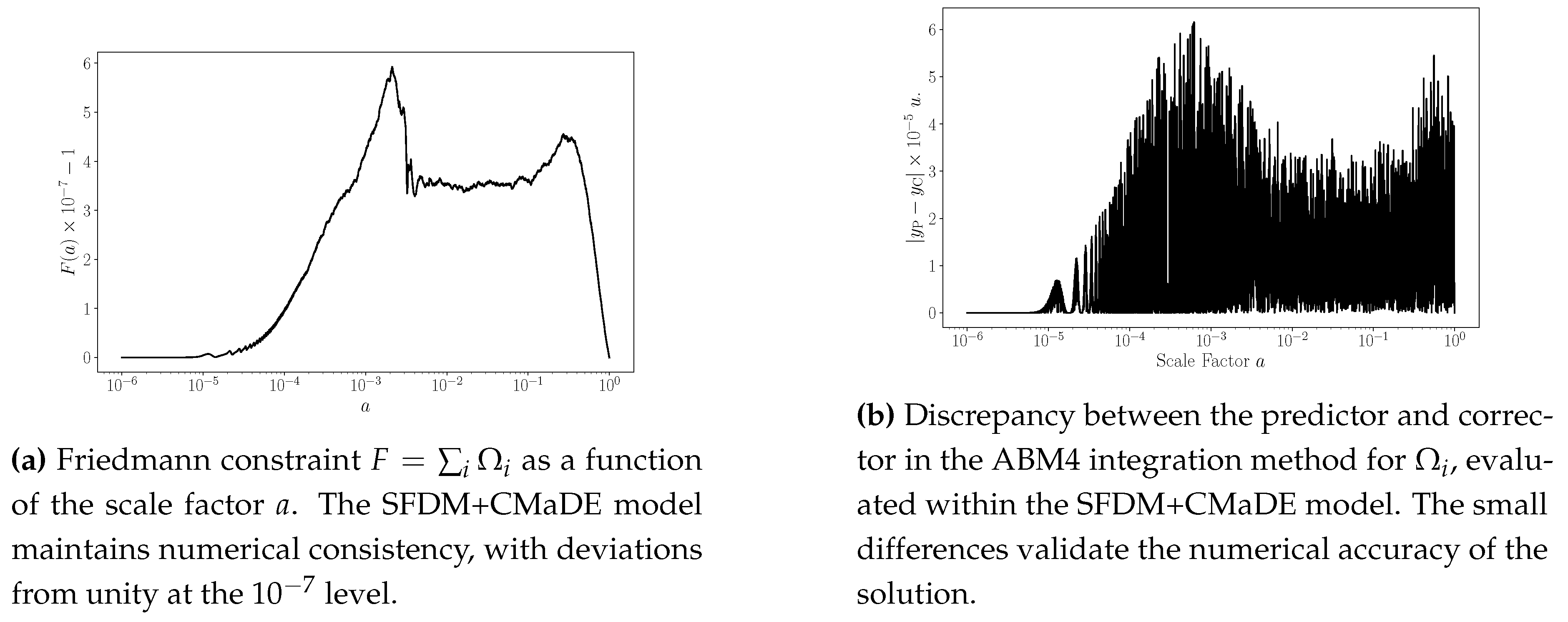
5.1. Numerical Treatment of CMaDE+SFDM

Incorporating the gravitational wave background through the CMaDE model introduces key modifications to the system of Equation (17). To account for these changes, we define the auxiliary quantity
l 1 3 M H ,
where the dark energy density is given by κ 2 ρ M = M c 2 . This definition allows us to reformulate the differential equation governing M (Equation (7)) in terms of the dimensionless variable l. After performing algebraic manipulations, the resulting expression takes the form:
l = 3 2 Π l + Q π 3 2 l 2 exp ( N ) .
Notably, the effect of CMaDE can be completely removed by setting k c = 0 , which restores a standard Λ CDM cosmology with a cosmological constant ( Λ ) as dark energy.
To explore how CMaDE affects dark matter dynamics, we analyze its impact on the evolution of the variables ( x , y ) , which describe SFDM. To facilitate interpretation, we introduce the transformation
x = Ω dm 1 / 2 sin ( θ / 2 ) , y = Ω dm 1 / 2 cos ( θ / 2 ) ,
following the formalism of [27]. Through additional algebraic development, we find that the Klein-Gordon (KG) equation acquires an extra term due to CMaDE, modifying its evolution equation:
x x 3 x + y y 1 + 3 2 Π x = Q π 3 2 k c l 3 exp ( N ) .
This result reflects a direct energy transfer between dark energy and dark matter, mediated in this scenario by the gravitational wave background (GWB) and the scalar field, respectively. Additionally, the Friedmann constraint equation is modified by the inclusion of an extra term:
Π = 2 Ω Φ sin 2 ( θ / 2 ) + 4 3 ( z 2 + ν 2 ) + b 2 + ( k c 1 ) Q π 2 3 l 3 exp ( N ) .
As before, setting Q = 0 nullifies CMaDE’s effect, returning the model to standard Λ CDM. Importantly, despite these modifications, the effective equation of state for dark energy, w eff , remains unchanged and continues to be given by Equation (8).
To systematically incorporate the energy transfer described in Equation (6), we now express the equations governing ( θ , Ω dm ) in the SFDM framework, incorporating the effects of CMaDE through Equations (20) and (22). The resulting system is:
θ = 3 sin ( θ ) + y 1 2 γ cot θ 2 ,
Ω Φ = 3 ( Π 1 + cos ( θ ) ) 2 γ Ω Φ ,
where we define the interaction parameter
γ = 3 2 Q π k c Ω Φ l 3 exp ( N ) .
With these modifications, the complete system of differential equations is given by Equations (17) and (24). We have solved these equations numerically using a custom-developed code, which is publicly available at https://github.com/edwphysics/SFDM-CMaDE.
Finally, to compute cosmological observables such as the CMB power spectrum and the matter power spectrum (MPS), we will use the Boltzmann solver CLASS [28]. For this, we build upon the existing implementation of SFDM in CLASS presented in [27], which we extend to incorporate the effects of CMaDE.

5.2. Initial Conditions

We evaluate the CMaDE+SFDM model using the ABM4 method, implemented in a custom-developed code that requires a specific set of initial conditions. Additionally, the ABM4 solution is incorporated into the CLASS code [28], necessitating the specification of initial conditions appropriate for this procedure. As discussed in Section 6, we compare the CMaDE+SFDM model with reference models: CMaDE+CDM, Λ SFDM , and Λ CDM, ensuring a uniform set of initial conditions for fair comparison. The expected behavior of key quantities during simulation should qualitatively align with the predictions of the reference model ( Λ CDM). However, minor adjustments to the initial conditions are necessary to ensure consistency across evaluated models. Notably, models incorporating CMaDE require higher curvature and a modified H 0 value to accurately recover the CMB and MPS observables.
As a first approximation, solutions using the ABM4 method are obtained by evolving backwards in time from a 0 = 1 to a i = 10 6 . This ensures that the ODEs are evaluated during crucial epochs, including the rapid oscillation phase of SFDM and key cosmological events such as the CMB decoupling ( a 10 4 ). The selected initial conditions are based on observational constraints from the Planck mission [29]. Accounting for nonzero curvature, the reference parameters at a 0 = 1 are as follows: the curvature density parameter Ω k 0 = 0.001, the Hubble constant H 0 = 100 h km / s / Mpc = 0.67, which corresponds to H 0 = 1.43 × 10⁻³³ eV in natural units ( c = = 1 ). Additional parameters include the baryon contribution Ω b 0 h 2 = 0.0224, total matter density (dark matter and baryons) Ω M 0 = 0.30, photon density Ω γ 0 h 2 = 2.47 × 10⁻⁵, and neutrino density Ω ν 0 h 2 = 1.68 × 10⁻⁵. The dark energy (DE) contribution is then determined via the Friedmann constraint:
Ω M 0 = 1 Ω b Ω D M Ω γ Ω ν Ω k .
The present-day value of the variable θ is determined by considering Equation (24). In this equation, the term y 1 = 2 m / H grows significantly at late cosmic times, including at t = t 0 , the current age of the universe. At this epoch, y 1 dominates the equation, leading to θ 2 y 1 , which implies θ ˙ 2 m . Consequently, integrating over time yields θ 2 m t . Using the universe’s age as given in the Λ CDM model [29] and the SFDM mass m = 10−22 eV, we obtain t = t 0 = 13.79 × 10⁹yrs = 6.61 × 1032 eV eV. Thus, the initial condition for the angular variable in the SFDM numerical formalism is:
θ 0 = 1.32 × 10 13 .

6. Results

6.1. Base Results: Λ SFDM Model

The numerical integration of the SFDM equations, as discussed in Section 5, provides a robust test for the ABM4 numerical scheme. The results confirm that the evolution of energy densities closely follows the expected Λ CDM trends. As seen in Figure 1a, radiation dominates until a 10 4 , transitioning into a matter-dominated phase up to a 0.5 , followed by the onset of dark energy domination. The relative deviations in Ω and H (Figure 1b,c) remain small, supporting the accuracy of the numerical solution.
A critical aspect of SFDM is its equation of state parameter, w Φ . As illustrated in Figure 2a, w Φ exhibits rapid oscillations around zero, ensuring that its time-averaged value remains w Φ 0 . This is a hallmark of SFDM, allowing it to behave as an effective dust component with ρ DM a 3 , aligning with standard cosmological predictions [27].
To verify the numerical accuracy of our simulations, we examine two key diagnostics: the Friedmann constraint F = i Ω i and the predictor-corrector discrepancy in the ABM4 scheme. Figure 3a shows that the Friedmann constraint is satisfied to high precision, with deviations below 10 6 , ensuring numerical stability. Additionally, the ABM4 corrector refines predictions within an error of | y P y C | < 10 5 (Figure 3b), further confirming the reliability of the numerical implementation.

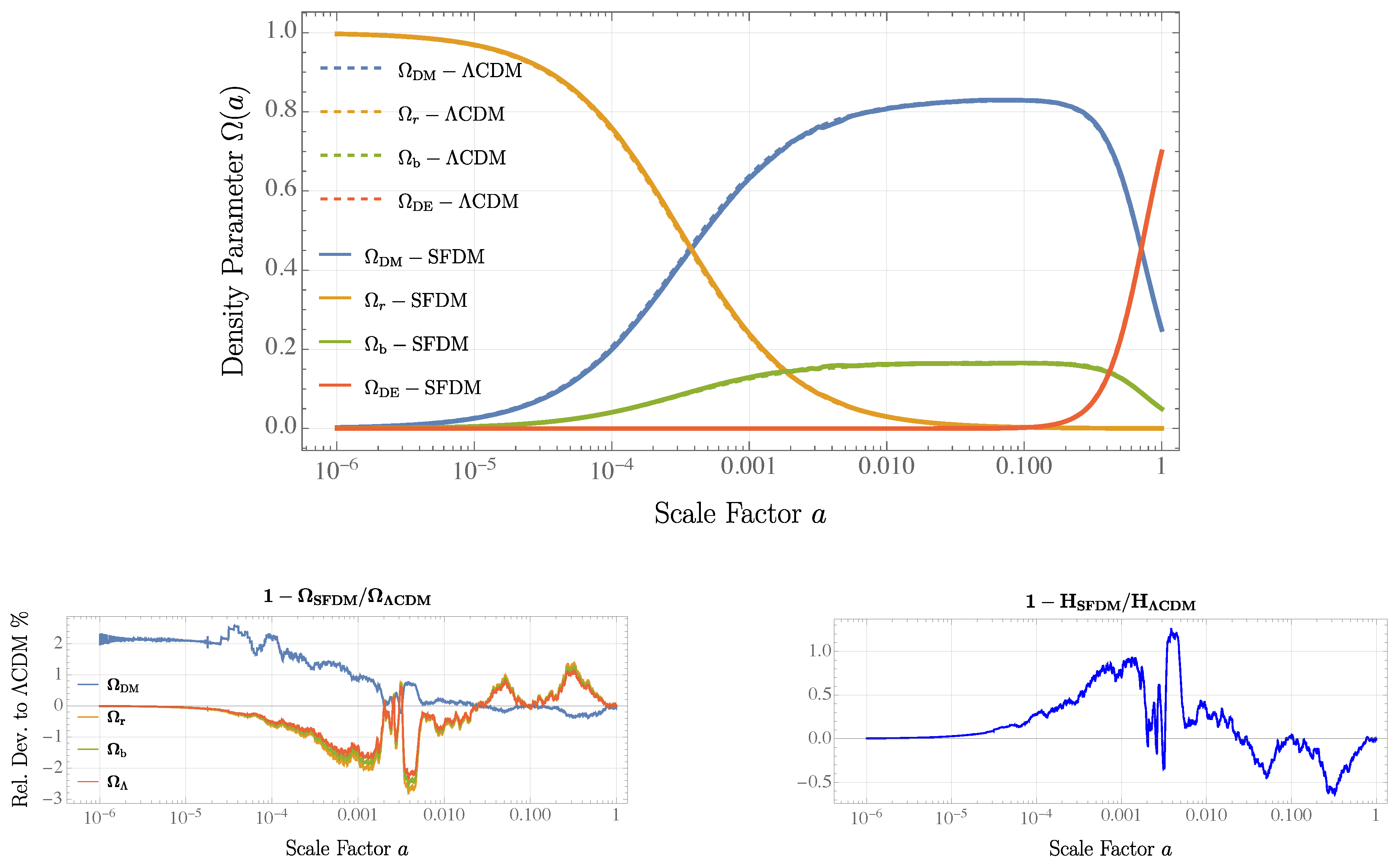
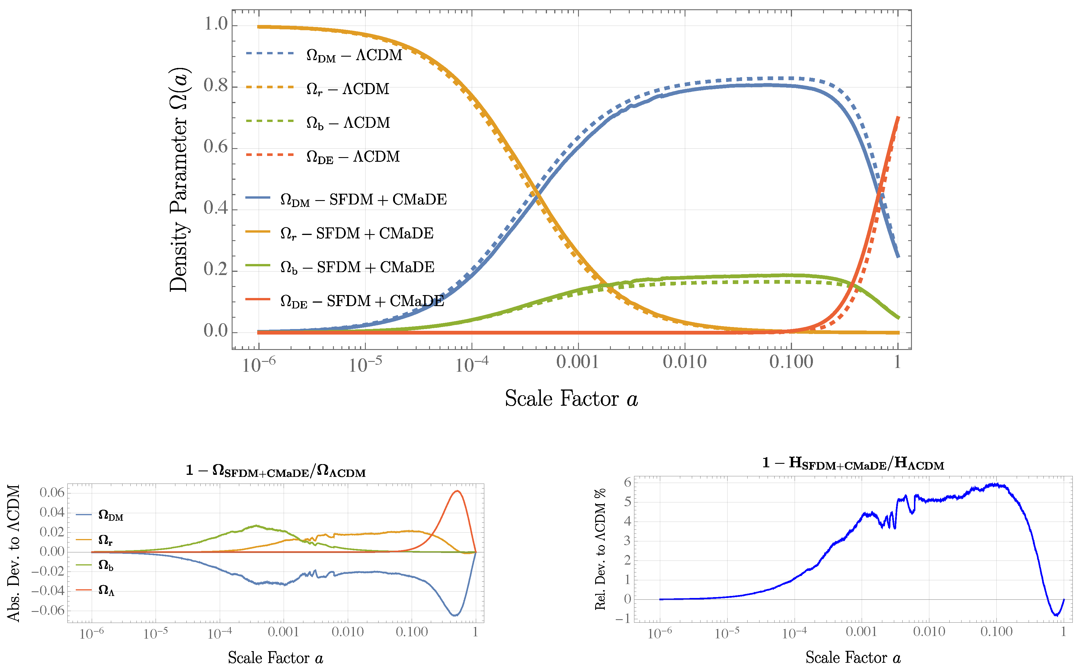
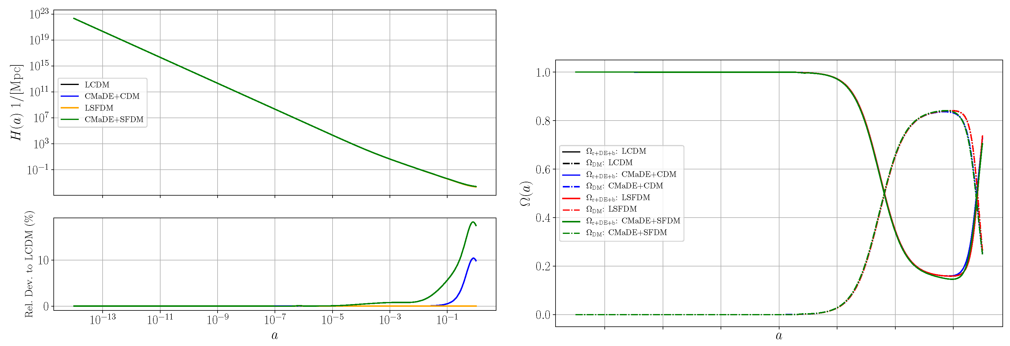
6.2. Cosmological Evolution in the CMaDE+SFDM Model

Introducing the CMaDE model into the SFDM framework leads to a subtle yet significant modification in the evolution of the energy densities. Figure 4a confirms that the general structure of the cosmic evolution remains unchanged, with radiation, matter, and dark energy domination phases occurring at the expected epochs. However, Figure 4b reveals a small but noticeable interaction between SFDM and the GWB-induced dark energy component for a 10 1 .
Figure 2b further supports the self-consistency of the SFDM+CMaDE model, showing that w eff converges to 1 at high redshift. This behavior is crucial for ensuring that the model remains compatible with observational constraints during recombination and beyond.
These findings validate the robustness of our numerical methods and confirm that the SFDM+CMaDE model remains a viable alternative to Λ CDM. The results presented here establish a solid foundation for further exploration, including perturbation analyses and their impact on structure formation, which will be discussed in the following sections.

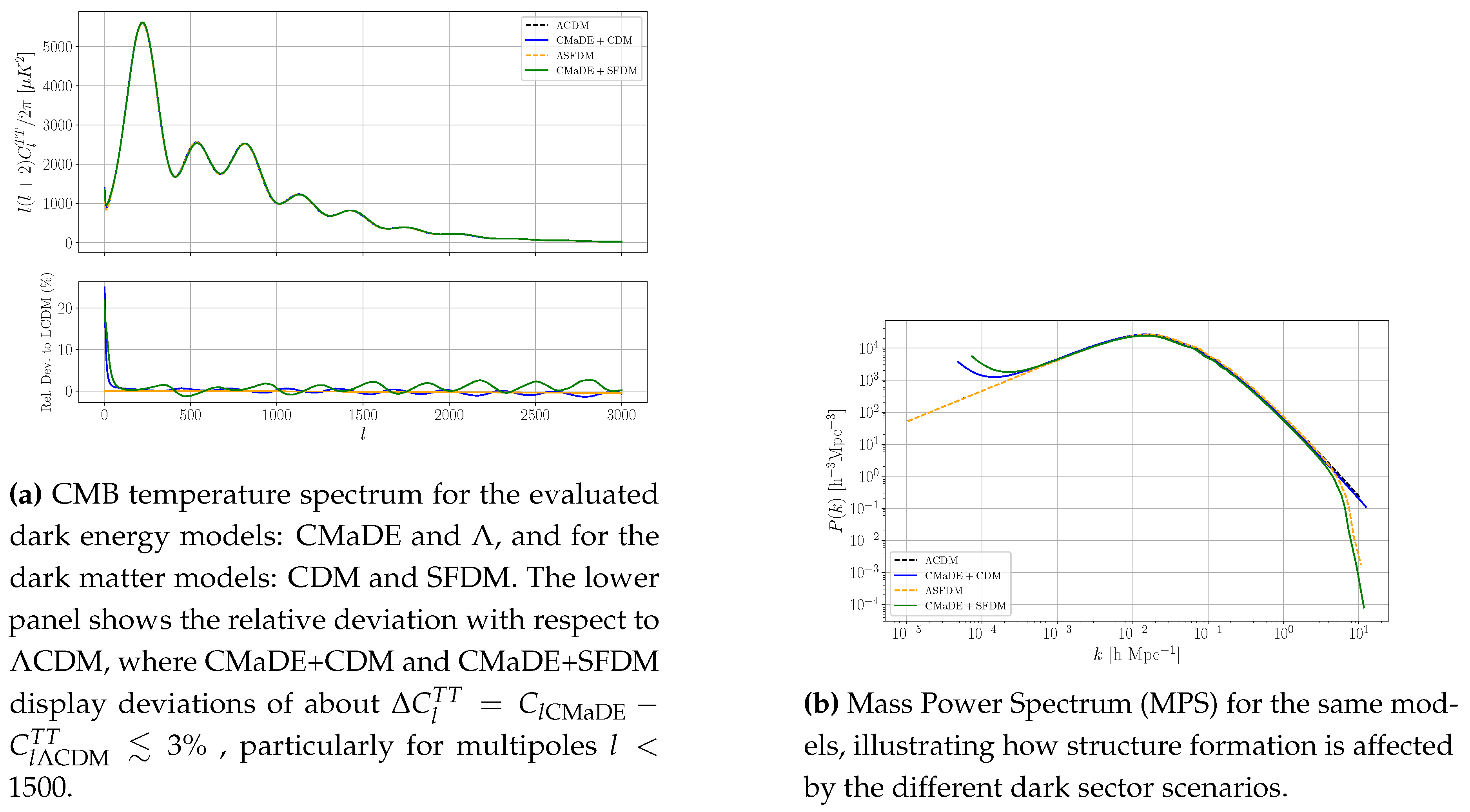
6.3. CMB and MPS Prediction

The cosmic microwave background (CMB) is one of the most precisely measured cosmological observables. Comparing observational data with theoretical predictions for the CMB is essential for assessing the validity of models describing dark energy and dark matter. In this section, we present the numerical results for the CMB and the Mass Power Spectrum (MPS), considering the GWB as a form of dark energy (CMaDE) and modeling dark matter as a scalar field. The methodology for obtaining these results using the CLASS code is detailed in Appendix A.
A similar pattern emerges in the MPS predictions, as shown in Figure 5b. The results for LCDM and LSFDM remain nearly identical, except for the expected cutoff at k 10 1 hMpc 1 , characteristic of SFDM models with a mass m Φ 10−22 eV. When introducing CMaDE as dark energy, whether combined with CDM or SFDM, the overall behavior remains consistent with their respective Λ -based counterparts, with minor variations primarily at k > 10 1 hMpc 1 .
The strong agreement between the CMB and MPS predictions for CMaDE, CDM, SFDM, and Λ suggests that all tested combinations remain viable. Notably, the CMaDE+SFDM model retains the essential characteristics to be considered a promising candidate for describing cosmic evolution. It is important to emphasize that CMaDE has been implemented in CLASS using a heuristic approach, meaning that further refinements, particularly in the numerical integration of the ODEs, are necessary. Interestingly, models incorporating CMaDE require H 0 > H 0 Λ CDM and Ω k > 0 . Specifically, the required values for the CMaDE+CDM and CMaDE+SFDM models are (H0 = 72.6 km s−1 Mpc−1, Ωk = 0.018) and (H0 = 77.0 km s−1 Mpc−1, Ωk = 0.048), respectively, to ensure consistency with the observed CMB and MPS results.
This need for adjustments is not unprecedented. Previous studies [30] have demonstrated that allowing for a nonzero curvature and an H 0 value differing from the Planck2018 prediction improves the agreement between CMaDE and Λ CDM. The results presented here indicate that CMaDE’s impact on the CMB follows a favorable trend, reinforcing the expectation that further refinements in the CMaDE+SFDM model could enable precise observational comparisons and a deeper assessment of its viability as a unified explanation for dark energy and dark matter.
Finally, Figure 6 presents the evolution of the density parameters Ω , as computed by CLASS under the chosen initial conditions, for different cosmic components as a function of the scale factor a. The results show that all models predict identical epochs of radiation, matter, and dark energy domination. However, models including CMaDE display slight deviations from the LCDM and LSFDM references during the dark energy-dominated epoch. This effect may stem from the energy transfer between dark matter and dark energy described in Equation (6).
This deviation is further evident in the Hubble parameter evolution shown in Figure 6, where a maximum deviation of approximately 10 % appears during the dark energy-dominated era for the CMaDE+CDM model. The effect is even more pronounced in the CMaDE+SFDM model, requiring an adjustment of nearly 20 % in H 0 during the late stages of cosmic evolution. This modification is crucial to match the reported CMB and MPS predictions. The implications and potential causes of this behavior will be explored further in Section 7.

7. Conclusions

This work explores an alternative cosmological framework where dark energy emerges as a gravitational wave background (CMaDE) [13] and dark matter is described by a scalar field (SFDM) [27]. To test this model, we numerically solve the governing equations (Equation (17)) using the fourth-order Adams–Bashforth–Moulton method and adapt the CLASS code to incorporate CMaDE, allowing us to compute the CMB temperature spectrum and the Mass Power Spectrum (MPS).
Our findings (Section 6) indicate that the CMaDE+SFDM model closely follows Λ CDM predictions for key cosmological observables, including the evolution of energy densities and the power spectra (Figure 5). However, achieving this agreement requires a higher Hubble constant ( H 0 ) and a small positive curvature ( Ω k ), specifically: (H0 = 77.0 km s−1 Mpc−1, Ωk = 0.048). A similar trend is seen in the CMaDE+CDM case: (H0 = 72.6 km s−1 Mpc−1, Ωk = 0.018), implying that CMaDE alters late-time cosmic expansion while preserving consistency with early-universe evolution [13].
Examining the evolution of H ( t ) (Figure 1c and Figure 4c), we find that SFDM alone already reproduces Λ CDM within a deviation of Δ H / H 1.26%, whereas incorporating CMaDE increases this difference to Δ H / H 5.97%. This suggests that CMaDE could help alleviate the Hubble tension, though it requires values of H 0 significantly higher than those reported by Planck [29].
Several caveats must be considered: i) the current CLASS implementation of CMaDE is heuristic and should ideally be replaced with direct numerical integration of the background equations; ii) while SFDM perturbations are accounted for, CMaDE perturbations are neglected, which may subtly affect the predicted spectra; iii) the parameter values used here require rigorous Bayesian inference for proper statistical validation. Despite these limitations, our results suggest that CMaDE+SFDM is worth further investigation.
Figure 2a,b confirm that the fundamental behavior of SFDM and CMaDE remains intact. SFDM effectively mimics CDM with ρ a 3 , while CMaDE exhibits a redshift-dependent equation of state, asymptotically approaching w eff 1 at high redshifts ( z > 10 6 ), ensuring consistency with early-universe observations.
Modeling dark energy as a GWB provides a natural coupling to both CDM and SFDM, though it systematically favors a larger H 0 than Λ CDM. Future observational campaigns, such as DESI and LSST, will be critical in testing this framework against precision cosmological data. However, the tension in H 0 and Ω k (H0 = 77.0 km s−1 Mpc−1, Ωk = 0.048) underscores the need for refined constraints.
Further progress requires improvements to the CLASS implementation, particularly by incorporating CMaDE perturbations, which could have subtle but important effects on CMB and MPS predictions. While our analysis has focused on large-scale cosmic evolution, an intriguing direction is the potential astrophysical implications of SFDM in galaxy formation and structure growth.
One of the most compelling aspects of CMaDE is its ability to reinterpret dark energy as a low-frequency GWB, introducing an additional term in Einstein’s equations that numerically behaves like the cosmological constant. This could provide an alternative explanation for cosmic acceleration, potentially offering a deeper theoretical understanding of dark energy.
The combination of CMaDE and SFDM presents a promising alternative to standard Λ CDM cosmology, bridging dark energy and dark matter into a unified framework. Recent gravitational wave background detections add further motivation to explore these ideas, possibly linking them to stochastic quantum theories [31].
The next decade promises significant advancements in cosmology, with new observational data poised to test models beyond Λ CDM. While CMaDE+SFDM remains a developing hypothesis, its theoretical foundations make it a strong contender for challenging the prevailing paradigm. The search for a deeper understanding of the universe continues.

Acknowledgments

The authors would like to express their gratitude to the Secretaría de Ciencia, Humanidades, Tecnología e Innovación (Secihti) for the financial support provided for this research project. We are particularly grateful for their commitment to education and scientific development in Mexico and Latin America. This work was also partially supported by CONACyT México under grants A1-S-8742, 304001, 376127, 240512.

Abbreviations

DM Dark Matter
DE Dark Energy
CMaDE Cosmic Microwave as Dark Energy
SFDM Scalar Field Dark Matter
GWB Gravitational Wave Background
EoS Equation of State
CDM Cold Dark Matter
CMB Cosmic Microwave Background
MPS Matter Power Spectrum

Appendix A. Interpolation of Energy Densities

The interpolations of ρ d m and ρ d e , which depend on the scale factor a, are essential for evaluating the impact of the CMaDE model on observables such as the CMB and the MPS, as well as the evolution of other relevant quantities in the universe within the CLASS framework. These energy densities were initially obtained through a custom code based on the ABM4 numerical method for solving ODEs, as described in https://github.com/edwphysics/SFDM-CMaDE. In this work, we focus on the interpolation of energy densities for the dark matter and dark energy components in the CMaDE+CDM and CMaDE+SFDM models. The interpolations were generated using the Fit[] module of Mathematica [32]. To integrate these interpolations into the modified CLASS code that includes the contribution from CMaDE, the energy density expressions were replaced as detailed in Appendix A. The precise forms of the interpolations for both models are discussed in this section.

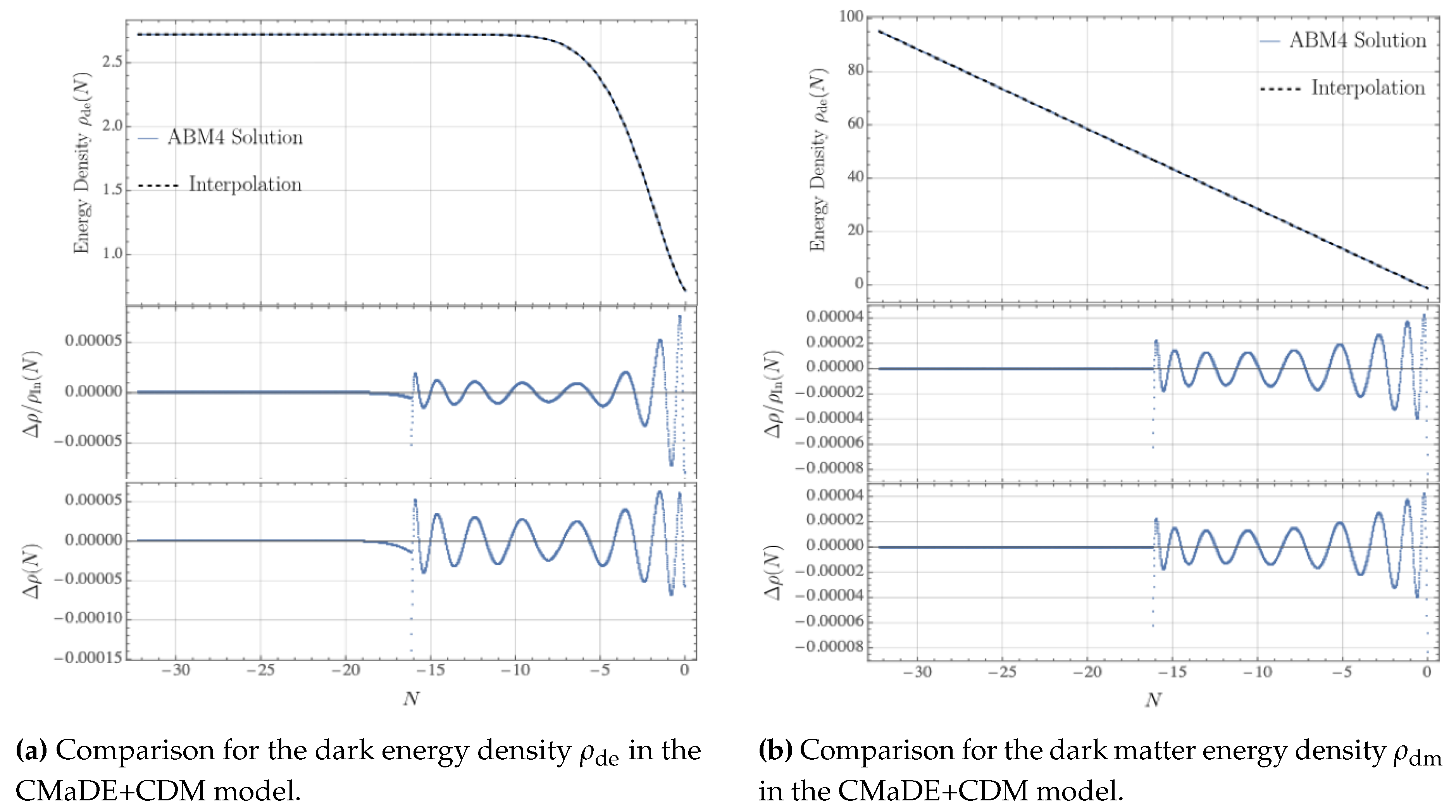
Appendix A.1. Interpolations in CMaDE+CDM

The CMaDE+CDM model provides a simple approach to incorporating the energy of the Gravitational Wave Background (GWB) into the evolution of the universe. It treats dark energy (DE) using the CMaDE model, as described in Section 2, and dark matter (DM) as Cold Dark Matter (CDM). In this model, the energy densities for both dark energy and dark matter are computed using the ABM4 method, with interpolations used to simplify the expressions.
For the dark energy density, the interpolation procedure yields a smooth functional form for the energy density ρ de . The interpolation is a power series expansion in terms of the e-folding variable N = log ( a ) , truncated to the 15th order. The choice of truncation order ensures that the interpolation remains accurate, with the absolute and relative errors between the ABM4 solution and the interpolation staying within sub-percent precision, as shown in Figure A1a.
Figure A1. Comparison between the ABM4 solution (dashed) and the interpolation (solid) of the energy densities in the CMaDE+CDM model. The top panels show the energy densities for dark energy (a) and dark matter (b), while the middle and bottom panels display the relative and absolute deviations between the ABM4 solution and the interpolation, respectively.
Preprints 150456 g0a1
Similarly, for the dark matter energy density ρ dm , the interpolation is also expressed as a series of terms that describe its dependence on N. This interpolation is similarly precise, as evidenced by the relative and absolute errors in Figure A1b. The precise interpolation of the energy densities for both DE and DM in the CMaDE+CDM model ensures a highly accurate and computationally efficient representation of the model’s energy components.
The middle and bottom panels of Figure A1a,b show the relative and absolute deviations between the ABM4 solution and the interpolation for the energy densities of dark energy and dark matter, respectively. These figures highlight the accuracy of the interpolation method used to model the energy densities in the CMaDE+CDM framework.

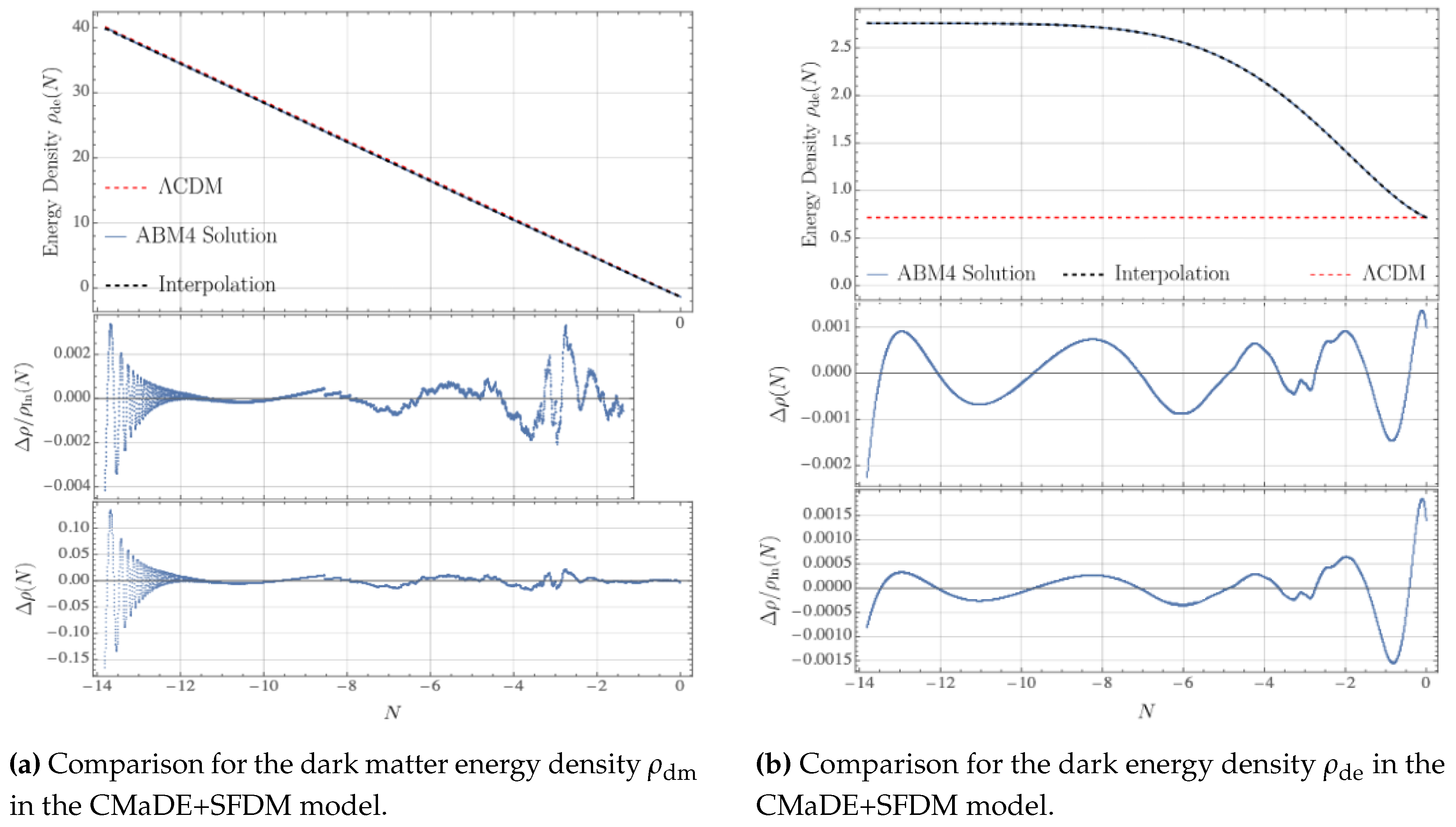
Appendix A.2. Interpolations in CMaDE+SFDM

In this case, the energy densities for dark matter (DM) and dark energy (DE) in the CMaDE+SFDM model were computed using the same interpolation procedure as in the previous section, based on the ABM4 solution. For both components, the interpolation method was applied to accurately capture the energy densities over a wide range of scale factor values. The interpolation was performed using a combination of polynomial and exponential functions, providing highly accurate results with sub-percentage precision. Notably, for both DE and DM, it was not necessary to truncate the polynomial expansions to very high orders, ensuring computational efficiency without compromising accuracy.
Figure A2. Comparison between the ABM4 solution (black dotted), the interpolation (solid), and the Λ CDM model (red dotted) for the energy densities of dark matter (a) and dark energy (b) in the CMaDE+SFDM model. The middle and bottom panels show the relative and absolute deviations between the ABM4 solution and the interpolation, respectively.
Preprints 150456 g0a2
The relative and absolute deviations between the ABM4 solution and the interpolation are shown in the figures, with the respective comparison also made to the Λ CDM model. These interpolations are important for understanding the evolution of the universe under the influence of both dark matter and dark energy in the CMaDE+SFDM model, and they are used within the modified CLASS code to evaluate observables such as the CMB and the MPS.

References

  1. Adame, A.; Aguilar, J.; Ahlen, S.; Alam, S.; et al. DESI 2024 VI: cosmological constraints from the measurements of baryon acoustic oscillations. Journal of Cosmology and Astroparticle Physics 2025, 2025, 021. [Google Scholar] [CrossRef]
  2. Adame, A.G.; Aguilar, J.; Ahlen, S.; Alam, S.; et al. DESI 2024 VII: Cosmological Constraints from the Full-Shape Modeling of Clustering Measurements, 2024, [arXiv:astro-ph.CO/2411.12022].
  3. Riess, A.G.; Yuan, W.; Macri, L.M.; et al. A Comprehensive Measurement of the Local Value of the Hubble Constant with 1 km s-1 Mpc-1 Uncertainty from the Hubble Space Telescope and the SH0ES Team. The Astrophysical Journal Letters 2022, 934, L7. [Google Scholar] [CrossRef]
  4. Koudmani, S.; Rennehan, D.; Somerville, R.S.; Hayward, C.C.; Anglés-Alcázar, D.; Orr, M.E.; Sands, I.S.; Wellons, S. Diverse dark matter profiles in FIRE dwarfs: black holes, cosmic rays and the cusp-core enigma 2024. arXiv:astro-ph.GA/2409.02172].
  5. Re, F.; Di Cintio, P. Structure of the equivalent Newtonian systems in MOND N-body simulations - Density profiles and the core-cusp problem. Astron. Astrophys. 2023, arXiv:astro-ph.GA/2307.08865]678, A110. [Google Scholar] [CrossRef]
  6. Matos, T.; Guzman, F.S.; Urena-Lopez, L.A. Scalar Field as Dark Matter in the Universe. Classical and Quantum Gravity 1999, 17, 1707–1712. [Google Scholar] [CrossRef]
  7. Matos, T.; Ureña-López, L.A.; Lee, J.W. Short review of the main achievements of the scalar field, fuzzy, ultralight, wave, BEC dark matter model. Frontiers in Astronomy and Space Sciences 2024, 11. [Google Scholar] [CrossRef]
  8. Hui, L.; Ostriker, J.P.; Tremaine, S.; Witten, E. Ultralight scalars as cosmological dark matter. Phys. Rev. D 2017, arXiv:astro-ph.CO/1610.08297]95, 043541. [Google Scholar] [CrossRef]
  9. Solís-López, J.; Guzmán, F.S.; Matos, T.; Robles, V.H.; Ureña López, L.A. Scalar field dark matter as an alternative explanation for the anisotropic distribution of satellite galaxies. Phys. Rev. D 2021, arXiv:astro-ph.GA/1912.09660]103, 083535. [Google Scholar] [CrossRef]
  10. Bernal, T.; Matos, T.; Hernandez, L.S. A natural explanation of the VPOS from multistate Scalar Field Dark Matter. JCAP 2025, arXiv:astro-ph.GA/2407.05273]01, 155. [Google Scholar] [CrossRef]
  11. Riess, A.G.; Filippenko, A.V.; Challis, P.; et al. Observational Evidence from Supernovae for an Accelerating Universe and a Cosmological Constant. The Astronomical Journal 1998, 116, 1009–1038. [Google Scholar] [CrossRef]
  12. Matos, T.; L-Parrilla, L. The graviton Compton mass as Dark energy. Revista Mexicana de Física 2021, 67. [Google Scholar] [CrossRef]
  13. Matos, T.; Escamilla, L.A.; Hernández-Marquez, M.; et al. Cosmology on a gravitational wave background. Monthly Notices of the Royal Astronomical Society 2024, 529, 3013–3019. [Google Scholar] [CrossRef]
  14. Agazie, G.; Anumarlapudi, A.; Archibald, A.M.; et al. The NANOGrav 15 yr Data Set: Evidence for a Gravitational-wave Background. The Astrophysical Journal Letters 2023, 951, L8. [Google Scholar] [CrossRef]
  15. Željko Ivezić; Kahn, S.M.; Tyson, J.A.; et al. LSST: From Science Drivers to Reference Design and Anticipated Data Products. The Astrophysical Journal 2019, 873, 111. [CrossRef]
  16. de Blok, W.J.G. The Core-Cusp Problem. Advances in Astronomy 2009, 2010, 789293. [Google Scholar] [CrossRef]
  17. Okamoto, T.; Frenk, C.S.; Jenkins, A.; Theuns, T. The properties of satellite galaxies in simulations of galaxy formation. Mon. Not. Roy. Astron. Soc. 2010, arXiv:astro-ph.CO/0909.0265]406, 208–222. [Google Scholar] [CrossRef]
  18. Newton, O.; Cautun, M.; Jenkins, A.; Frenk, C.S.; Helly, J. The total satellite population of the Milky Way. Mon. Not. Roy. Astron. Soc. 2018, arXiv:astro-ph.GA/1708.04247]479, 2853–2870. [Google Scholar] [CrossRef]
  19. Pawlowski, M.S.; Kroupa, P.; Jerjen, H. Dwarf galaxy planes: the discovery of symmetric structures in the Local Group. Monthly Notices of the Royal Astronomical Society 2013, 435, 1928–1957. [Google Scholar] [CrossRef]
  20. Pawlowski, M.S.; Kroupa, P. The Milky Way’s disc of classical satellite galaxies in light of Gaia DR2. Monthly Notices of the Royal Astronomical Society 2020, 491, 3042–3059. [Google Scholar] [CrossRef]
  21. Matos, T.; Guzman, F.S. Scalar fields as dark matter in spiral galaxies. Class. Quant. Grav. 2000, 17, L9–L16. [Google Scholar] [CrossRef]
  22. Hui, L.; Ostriker, J.P.; Tremaine, S.; et al. Ultralight scalars as cosmological dark matter. Physical Review D 2017, 95, 043541. [Google Scholar] [CrossRef]
  23. Matos, T.; Ureña-López, L.A. A Further Analysis of a Cosmological Model of Quintessence and Scalar Dark Matter. Physical Review D 2000, 63. [Google Scholar] [CrossRef]
  24. Matos, T. The quantum character of the Scalar Field Dark Matter. Monthly Notices of the Royal Astronomical Society 2022, 517, 5247–5259. [Google Scholar] [CrossRef]
  25. Ureña-López, L.A. Brief Review on Scalar Field Dark Matter Models. Frontiers in Astronomy and Space Sciences 2019, 6, 438500. [Google Scholar] [CrossRef]
  26. Matos, T.; Ureña-López, L.A. Further analysis of a cosmological model with quintessence and scalar dark matter. Physical Review D 2001, 63, 063506. [Google Scholar] [CrossRef]
  27. Ureña-López, L.A.; Gonzalez-Morales, A.X. Towards accurate cosmological predictions for rapidly oscillating scalar fields as dark matter. Journal of Cosmology and Astroparticle Physics 2016, 2016, 048–048. [Google Scholar] [CrossRef]
  28. Lesgourgues, J. The Cosmic Linear Anisotropy Solving System (CLASS) I: Overview. ArXiv 2011. [Google Scholar]
  29. Aghanim, N.; Akrami, Y.; Ashdown, M.; Planck 2018 results -, VI.; et al. Cosmological parameters. Astronomy & Astrophysics 2020, 641, A6. [Google Scholar] [CrossRef]
  30. Matos, T.; Tellez-Tovar, L.O. The cosmic microwave background and mass power spectrum profiles for a novel and efficient model of dark energy. Revista Mexicana de Física 2022, 68, 020705–1. [Google Scholar] [CrossRef]
  31. Escobar-Aguilar, E.S.; Matos, T.; Jimenez-Aquino, J.I. On the physics of the Gravitational Wave Background 2023.
  32. Inc., W.R. Mathematica, 2024.
Figure 1. Comparison of key cosmological parameters in the SFDM model without the GWB. (a) Evolution of the density parameters Ω for different components: Ω DM (scalar field dark matter), Ω DE (dark energy as a cosmological constant), Ω ν (relativistic neutrinos), Ω γ (radiation), and Ω b (baryonic matter) over the scale factor a. (b) Relative error in Ω compared to the Λ CDM model. (c) Relative deviation in the Hubble parameter H between the SFDM and Λ CDM models, with a maximum discrepancy of 1.26% for H and 2.57% for Ω .
Preprints 150456 g001
Figure 2. Equation of state parameters for SFDM (fig:wphiVa-SFDM-UGD) and CMaDE (fig:weffVz-SFDM+CMaDE-UGD).
Preprints 150456 g002
Figure 3. Comparison of numerical consistency in the SFDM+CMaDE model. (Left) The Friedmann constraint remains accurate within a deviation of 10 7 . (Right) The predictor-corrector discrepancies validate the numerical solution.
Preprints 150456 g003
Figure 4. Comparison of the SFDM+CMaDE model with Λ CDM. (a) Evolution of density parameters Ω i . (b) Relative error in Ω i compared to Λ CDM. (c) Relative deviation in the Hubble parameter H, with a maximum difference of 5.97% for H and 13.09% for Ω i .
Preprints 150456 g004
Figure 5. Comparison of key cosmological observables for the evaluated dark energy and dark matter models. (Left) CMB temperature spectrum and its relative deviation from Λ CDM. (Right) Mass Power Spectrum (MPS), highlighting the impact on structure formation.
Preprints 150456 g005
Figure 6. (Left) Hubble parameter evolution for the evaluated dark energy models: CMaDE and Λ , and for the dark matter models: CDM and SFDM, showing how different scenarios impact cosmic expansion. (Right) Density parameters for the same models, illustrating the evolution of the dark energy and dark matter components throughout cosmic history.
Preprints 150456 g006
Disclaimer/Publisher’s Note: The statements, opinions and data contained in all publications are solely those of the individual author(s) and contributor(s) and not of MDPI and/or the editor(s). MDPI and/or the editor(s) disclaim responsibility for any injury to people or property resulting from any ideas, methods, instructions or products referred to in the content.
Copyright: This open access article is published under a Creative Commons CC BY 4.0 license, which permit the free download, distribution, and reuse, provided that the author and preprint are cited in any reuse.
Prerpints.org logo

Preprints.org is a free preprint server supported by MDPI in Basel, Switzerland.

Subscribe

Disclaimer

Terms of Use

Privacy Policy

Privacy Settings

© 2025 MDPI (Basel, Switzerland) unless otherwise stated