
Submitted:
24 February 2025
Posted:
25 February 2025
You are already at the latest version
Abstract
Urban biodiversity is essential for sustainable cities, as it helps address the challenges of environmental degradation, ecosystem loss, species decline, and increased vulnerability to climate hazards, which negatively affect human health and well-being. ECOLOPES (ECOlogical building enveloPES) aims to develop a design approach for multi-species as stakeholders to achieve regenerative urban ecosystems. Integrating the diverse data required for stakeholders and beyond-spanning life sciences, geography, and architecture-and utilizing it for design presents a significant challenge. This paper introduces an ontology-driven approach that utilises ontology-based data management (OBDM) as a framework for integrating diverse data sources, enabling ecologists and architects to design sites and buildings that foster urban biodiversity. OBDM offers a unified view of multiple data sources through an ontology, enabling query and update operations to be performed directly on the integrated data. The proposed ontology, developed in collaboration with domain experts and adhering to Semantic Web and Linked Data best practices, serves as a mediator between life sciences data (e.g., species distribution and habitats) and geometric information (e.g., maps, voxel models of building structures). This integration enables the adaptation of site, buildings and geometries respectively to create habitats that attract and support urban wildlife, contributing to ecological sustainability. The paper illustrates the practical utility of the ontology through a case study, highlighting its role in guiding building designs that promote species attractiveness and urban biodiversity.
Keywords:
ontology-based data access
; knowledge graphs
; urban biodiversity
; sustainable building design
1. Introduction
The expansion of urban areas, and the resulting decline in natural spaces, has led to new challenges, including ecosystem degradation, species loss, and increased vulnerability to climate hazards among others. Urban biodiversity is essential for sustainable cities, as it helps address the challenges, which negatively affect human health and well-being. ECOLOPES (ECOlogical building enveloPES), an H2020 FET Project, aims to develop a design approach for multi-species as stakeholders to achieve regenerative urban ecosystems [1]. With multi-species we mean four different types of inhabitants that can co-occupy the envelope: plants, animals, microbiota and humans.
Integrating the diverse data required for stakeholders and beyond—spanning life sciences, geography, and architecture—and utilizing it for design presents a significant challenge. This paper introduces an ontology-driven approach that utilises ontology-based data management (OBDM) [2] as a framework that integrates diverse data sources, enabling ecologists and architects to design sites and buildings that foster urban biodiversity. Proposed ontology-aided design methodology builds up on the concept of performance-oriented design [3,4] and the conceptual framework focused on data-driven approaches to understanding and designing environments [5].
Data sources range from publicly available datasets, which can be easily accessed and retrieved via web APIs—such as GLoBI (Global Biotic Interactions for species) [6]—to private datasets generated within ECOLOPES, including Plant Functional Groups (PFGs) [7], Animal Functional Groups (AFGs), and voxel data [8] that capture site-specific variables like coordinates, aspect, slope, or solar radiation. Plant and animal functional groups, defined by shared traits or ecological roles rather than taxonomic classification, play a crucial role in ecosystem processes, resilience, and biodiversity conservation. Voxel model contains useful aggregated information applicable to various use cases, such as computing the Habitat Suitability Index (HSI), a model which evaluates how well a habitat suits a given species. Therefore, depending on the weighting scheme employed by the respective specific publication or study on the reported species (e.g., rabbit, fox), one can calculate and infer for each point in CAD environment how suitable it is for the designated species with respect to environmental conditions in voxel model: aspect, slope, elevation, solar radiation and so forth. Another dimension of data emerges from the designer’s interaction with CAD and Grasshopper environments. In this environment, the designer based on the project brief requirements creates a network configuration by using predefined `circle shapes’ of EcoNodes (denoting species) and ArchiNodes (denoting buildings or other architectural objects).
The resulting desperate and heterogeneous data requires integration, alignment, and consolidation into a unified RDF-based graph data model, with ontological terms used to define the mappings. The result is a knowledge graph [9,10] that contains curated and contextualized knowledge, enabling holistic querying and answer retrieval through the use of domain ontologies. In order to implement it, we have employed OBDM–an extension of Ontology-based data access (OBDA) [11] with support for updates [12] in addition to queries–as a data integration framework. This approach led to some data being virtualised (e.g., voxel model), while the remaining data was materialized, i.e., stored and consequently indexed by the triple store. This approach is pragmatic as the data is not moved as well as no data duplication is created, albeit with the general downside of reduced performance in query evaluation. Nonetheless, subject to performance indicators or providing a seamless workflow for the designer a (subset of) voxel data can be materialised in order to meet the required interaction criteria [13]. For instance, in our case the Euclidian distance between two Nodes is a candidate for pre-materialisation to increase the performance of the query, typically viable in cases where changes to the position of Nodes do not occur frequently.
The scope of the knowledge graph is often determined by the set of competency questions (CQs) [14] it is designed to answer, such as “Provide me with the local species that are known to have the protection status threatened.” To achieve this, new data must be ingested, such as public data on local species provided by municipalities, citizen science (e.g. GBIF1), and threatened species data from International Union for Conservation of Nature (IUCN)2. Additionally, this data often requires alignment across datasets—for instance, by linking data referring to the same entity using owl:sameAs assertions or custom relationships defined within the ontology. In this case, the species latin name alongside species taxonomic rank (if applicable) can be leveraged in order to perform the disambiguation process, and therefore aid in the alignment process between entities.
Ontologies, particularly those built using OWL3 (Web Ontology Language), not only provide a comprehensive description of a domain but also enable the inference of new implicit facts (i.e., RDF triples) based on the explicit facts asserted in the knowledge graph. Domain experts and ontologists often aim to reuse concepts from existing ontologies or establish alignments to create more expressive and granular structures, which can be leveraged on demand or to support reasoning capabilities using Open World Assumption (OWA). In our case, we have modeled ECOLOPES ontology using a top-down conceptualization, a bottom-up approach informed by the data, and by reusing structures from well-established ontologies, namely OBO Relations [15] or Darwin Core4 following ontology construction best practices.
The proposed ontology, developed in collaboration with domain experts and adhering to Semantic Web and Linked Data best practices, serves as a mediator between life sciences data (e.g., species distribution and habitats) and geometric information (e.g., maps, voxel models of building structures). The ontology is an interface with CAD and aids the design of ecological building envelopes addressing the critical “data-to-design gap” [16,17] in computational architecture and multi-species architectural design.
Constraints, unlike ontologies–that are designed for logical, deductive reasoning–adhere to the Closed World Assumption (CWA), precisely defining how data should be structured by imposing specific restrictions on the data model. In our case, constraints are represented as explicit facts in the knowledge graph, such as the solar requirements of plants or the minimum and maximum proximity distances between species. By using standards like SHACL5, one can define and validate the expected “shapes” and structure of the data, ensuring data quality and completeness while also enabling the enforcement of consistency across the dataset. In our case, currently the validation is performed using a set of SPARQL queries. The constraints in our problem setting can be translated to SPARQL queries, e.g. “Provide me the locations in site where I can place the plant Abies Alba (EcoNode) such that its solar requirements are met?”. Given the spatial nature of this query, typically one would employ a GeoSPARQL query to answer it; nonetheless, in our case because of voxel model containing x, y, z coordinates boils down to equality checking with respect to CAD coordinates.
The computational model that is used to generate design outcomes based on the designer’s input is rule-based. This approach computes the design outcomes based on the selected rules that can be run in a designated order. Our current implementation mimics a rule-based reasoning by employing a set of SPARQL update queries [18] in the context of OBDM that are run in a sequence that is orchestrated by the Grasshopper environment.
This integration enables the adaptation of site, buildings and geometries respectively to create habitats that attract and support urban wildlife, contributing to ecological sustainability. The paper illustrates the practical utility of the ontology through a (case study) demonstrator, highlighting its role in guiding building designs that promote species attractiveness and urban biodiversity.
Our contributions are:
- A new EIM (ECOLOPES Information Model) ontology and knowledge graph in the domains of architecture and ecology.
- A method based on OBDM to map and integrate different data sources stemming from different environments from the respective domains.
- A designer workflow in which the designer is getting feedback (e.g. fulfillment of solar radiation or proximity constraints) or ask CQs against the KG.
The rest of the paper is structured as follows. In Section 2 we provide the necessary background, motivation and problem statement. In Section 3 we discuss related work in respect to using the ontologies in design and ecology. In Section 4 we explain the ontology design, reuse and alignment. In Section 5 we discuss the data integration framework used for integrating the heterogeneous data sources. In Section 6 we describe the demonstrator and we provide the results achieved in that context. And, finally in Section 7 we conclude the paper with conclusions and future work.
2. Motivation and Problem Statement
The ontology-aided generative computational design process facilitates design generation, namely of the search space populated with alternative design solutions that can be analysed and evaluated. The overall process of design generation entails synthesising heterogeneous ecological, environmental, and architectural data, voxel-based data structuring, context-information at regional/urban and local/architectural scales, and modeling information according to decision needs.
The role of the ontologies is to model information regarding the entities and relationships that need to be represented and to aid the design of ecological building envelopes. We distinguish between ontologies as schema TBox and instance data as ABox. More formally, for a given data source and its variables x we create ABox by applying a set of mappings: , where E is a TBox class or property, is a set of IRI templates, each applied to the variable x in order to create a Literal or IRI. Knowledge graph KG is union of ABox and TBox6, represented in RDF and typically stored (materialised) in a triple store. To avoid the complexity of reification statements in RDF, we choose to model statements using RDF-star for convenience, namely for expressing proximity constraints. A (part of) ABox can be virtualised instead of being materialised depending on the use case requirements. In this particular case, the mappings ⇝ that are represented in a specific mapping language are used to translate the queries on the fly back to the original data sources. TBox axioms are used to infer new implicit triples in ABox based on asserted (ABox) triples, which are either stored in the triple store, or alternatively query is rewritten during the query time with respect to TBox axioms to account for the same (query) answers. This proposition does not hold for expressive OWL ontology languages, but rather for (minimal) RDFS, consisting of domain/range, subClassOf and subPropertyOf axioms [12,19]. For such pragmatic reasons we use (minimal) RDFS in conjunction with a few OWL axioms (e.g. for aligning properties via owl:equivalentProperty) for the task of ontology modeling. In the case of OBDA and mappings, aside query rewriting an additional step of query unfolding is executed in which SPARQL queries are translated on the fly to SQL queries in order to obtain the so-called certain query answers [20]. OBDM extends OBDA with support for update queries.
The role of the voxel model within the ontology-aided design process is to structure and spatialize datasets describing the real-world location in which the design process is taking place. Based on an extensive literature review of the voxel models’ role in the engineering fields [8], an early definition of voxel models as "knowledge representation schemata" [21] was established in the context of computational design. Voxel model implementation developed for this study extends the Composite Voxel Model methodology [22] to incorporate the explicit link with the knowledge representation through the ontology-aided design process. The implemented ECOLOPES Voxel Model contains data describing the real-world site’s physical geometry and environmental performance. Currently, voxel-based design approaches addressing anthropogenic landscape adaptations can be found [23], and studies aiming to integrate voxel and ontological modeling are ongoing [24]. The presented implementation of the ECOLOPES Voxel Model is unique since it operates in the relational database environment (PostgreSQL), providing the implemented EIM Ontology with direct access to voxel data through the native “OBDA” mappings. As indicated in Figure 1, datasets provided by the ECOLOPES Voxel Model are structured as voxel data layers. Currently raw, aggregate and filtered data layers are exposed in the EIM Ontologies, enabling interactive temporal resolution change of the environmental simulation data contained in the ECOLOPES Voxel Model (cf. Figure 2). For example, existing data describing monthly average sunlight exposure can be aggregated to create five additional data layers. Those layers represent average sunlight exposure (sunlight hours) in summer, autumn, winter, spring and in the growing season. Designers can retrieve voxel data, including geometry and all available parameters, stored in different levels that represent different scales and resolutions, which are exposed as a SPARQL endpoint (see Section 5).
Two processes are combined in the ontology-aided generative computational design process: (i) the translational, and (ii) the generative process.
In the translational process the designer analyses, correlates, and locates spatially architectural and ecological requirements contained in the design brief, and design-specific determinations, while taking into consideration relevant constraints (i.e. as given by planning regulations). In order to do so, the designer uses a set of predefined Nodes and places them in the CAD environment in order to satisfy ecological and architectural requirements. Herein, the designer can query the knowledge graph in order to get feedback regarding the solution space regarding permissible design outputs, in terms of satisfying the proximity distances between Nodes (e.g. species) or solar radiation requirements. Nodes that fulfil the constraints are depicted as green circles, whereas the ones that do not are depicted as red crosses. Grasshopper environment is used as a component for doing the orchestration process of the validation. Knowledge graph is also a mediator with the voxel model (cf. Figure 1) that contains prepared datasets regarding geometric and environment variables. In this paper we focus on the translation process only. The intended goal of the translational process is shown in Figure 3.
The generative process consists of two distinct stages. In the first stage, the variations of spatial organisation are generated and evaluated. In the second one, specific surface geometries are generated for selected outputs of the previous stage and evaluated according to defined criteria, i.e. key performance indicators. The generative process falls outside the scope of this work and is planned for future exploration.
3. Related Work
The use of Semantic Web technologies and OWL to represent ecological network specifications is explored in [27]. Ecological networks capture the structure of existing ecosystems and provide a basis for planning their expansion, conservation, and enhancement. An OWL ontology is employed to model these networks, enabling reasoning about potential improvements and identifying violations in proposed network expansions. The approach incorporates a language called GeCoLan to define ecological network specifications, which are subsequently translated into GeoSPARQL queries. This methodology enhances the planning and management of ecological networks by supporting automated reasoning and integrating diverse data sources effectively.
Global Biotic Interactions (GLoBI) [6] is an open-access platform designed for researchers, aggregating diverse datasets to provide comprehensive information on species interactions, such as predator-prey, pollinator-plant, and parasite-host relationships, among others. The platform serves as a valuable resource for understanding ecological networks, predicting the effects of environmental changes, and guiding conservation strategies. It consolidates and harmonizes data on species, their occurrences, and interactions from a variety of publications and observational databases. GLoBI offers both an API and a SPARQL endpoint (with partial data coverage) for accessing species interaction data in CSV or RDF formats. Species data is structured using the Darwin Core7 vocabulary, with equivalence between species established through owl:sameAs relations. Additionally, the platform features a web-based frontend application that supports species searches via text and/or geographical boundaries. The OBO Relations8 ontology can be leveraged for reasoning to infer implicit interactions based on explicitly recorded triples.
The integration of ontologies and knowledge graphs in urban ecology has gained significant attention due to their ability to model complex interactions between built environments and natural ecosystems [17]. Existing research spans two major domains: Architecture, Engineering, and Construction (AEC(O)) and Urban Design, Planning, and Management, both of which are crucial for advancing sustainable urban development. Ontologies and knowledge graphs have been extensively used in AEC(O) to improve data interoperability, lifecycle management, and decision support systems. In Building Modelling, semantic models such as the Industry Foundation Classes (IFC) ontology enable structured data exchange across different software platforms [28]. In Building Construction and Renovation, ontologies assist in process optimization, cost estimation, and resource planning by integrating heterogeneous datasets [29]. Additionally, Building Automation has benefited from ontologies like the Brick schema, which enables semantic representation of building sensors and control systems. Ontologies also play a key role in Building Sustainability, facilitating the assessment of energy efficiency and carbon footprints [30]. Semantic models allow for the integration of green building certification standards (e.g., LEED, BREEAM) with real-time building performance data, enhancing decision-making for sustainable design and renovation [31]. Ontologies have been applied in City Modelling, enhancing urban digital twins with semantic interoperability [32]. The CityGML standard, extended with ontologies, provides a structured representation of urban elements, supporting applications in Civil Construction and infrastructure management. Urban Sustainability ontologies enable the integration of environmental indicators with urban planning tools, aiding in decision-making for reducing ecological footprints [33]. The role of Urban Green and Blue Infrastructure ontologies is particularly relevant for urban ecology. These semantic models capture the relationships between natural elements (e.g., vegetation, water bodies) and built environments, supporting biodiversity monitoring and ecosystem services assessment [34]. While AEC(O) and urban planning ontologies provide structured models for specific domains, their integration with ecological and functional dimensions is essential for advancing sustainable urban ecosystems. Several key research areas highlight the necessity of interlinking these domains: Simulation, where ontologies enable multi-domain simulations for energy performance [35], microclimate analysis, and species habitat suitability within urban environments [36]; Garden Management, where knowledge graphs integrate urban vegetation data with soil conditions, climate factors, and biodiversity metrics, improving urban green space management [37]; Urban Key Performance Indicators (KPIs), where ontologies facilitate KPI-based urban sustainability assessments by structuring data on air quality, noise pollution, and resource efficiency [38]. Despite advances in these areas, challenges remain in harmonizing ontologies across domains, ensuring scalability, and developing reasoning mechanisms that enhance automated decision support.
4. Ontology Design and Development
In this section, we outline the ontology development process for EIM following W3C best practices and FAIR principles. The process begins with defining requirements through expert input and competency questions (CQs). Next, terms and axioms are created, ensuring reuse of existing vocabularies for interoperability. The ontology is then structured and formalized, followed by validation and visualization to enhance accessibility and usability.
4.1. Defining the Ontology Requirements
We organized a collaborative workshop with experts from the Ecolopes consortium, comprising architects and ecologists, to define the ontology and knowledge graph requirements. Given that most participants were not ICT specialists or knowledge engineers, identifying and conceptualizing ontology requirements posed a significant challenge. To facilitate this process, we structured the workshop around ontology construction best practices, ensuring that domain experts could systematically contribute their knowledge in a way that aligns with semantic modeling principles.
Participants were divided into four interdisciplinary teams to encourage “cross-pollination” of ideas, leveraging diverse expertise to bridge conceptual gaps. Each team was tasked with defining a comprehensive set of competency questions (CQs) spanning both domains, a fundamental step in ontology engineering that helps capture the intended scope and use cases. These CQs were written on post-it notes to foster discussion and iterative refinement, allowing experts to progressively articulate their knowledge in a structured manner.
In parallel, participants identified key concepts and relationships relevant to answering the CQs, mapping out the foundational elements of the ontology. However, the abstraction required for formal ontological representation proved difficult for non-ontology experts. To mitigate this, they were guided to propose synonyms, group related concepts into broader categories, and outline hierarchical relationships, effectively shaping the initial class taxonomy. Recognizing that defining structured properties and attributes requires a technical perspective, we encouraged participants to describe informal connections between concepts, which were later formalized by knowledge engineers. When gaps remained in structuring the ontology, participants suggested relevant datasets or external sources that could support answering the identified CQs, ensuring that the ontology remained grounded in real-world data and met FAIR principles for interoperability and reusability.
This bottom-up, expert-driven approach resulted in a draft skeleton ontology, comprising initial classes, properties, and attributes.
Requirements were captured through CQs, to name a few:
- Which species we want/don’t want to attract close to our building?
- Which species are in PFG herbs_3?
- Which species that colonize the building are protected?
- Which species are invasive in this location?
- Which species can reach or live on sloped surfaces?
- What is the soil depth required for PFG herbs_3?
4.2. Ontology Requirements and Scope
One of the main ontology aims is to integrate diverse data sources to support sustainable building design decisions that enhance urban biodiversity. Its scope includes ecological data (e.g., species distribution and habitat preferences), architectural data (e.g., building geometry and materials), and geographical data (e.g., environmental conditions and maps). By facilitating data interoperability and enabling reasoning capabilities, the ontology seeks to inform ecologists and architects in designing buildings that foster ecosystem development.
Once the definition phase of CQs has been finished, the next steps were to group them based on similarity and prioritize based on importance. After the screening and processing of the CQs has been performed, we could extract general (i.e. upper level) requirements out of those. In the scope of this paper, we consider that processing of all CQs is out of scope, hence herein we focus only on general constraints and requirements that pertain to:
- Proximity between architectural objects and species (and vice versa), or likewise between species only.
- Solar radiation (regarding species).
- Prey areas in CAD environment, which denote areas that species are allowed to prey on one another.
4.3. Ontology Creation Process
The ontology9 was developed following Semantic Web and Linked Open Data (LOD) best practices, ensuring compliance with the FAIR (Findable, Accessible, Interoperable, Reusable) principles. The methodology employed a structured approach incorporating:
- Iterative design and refinement, integrating feedback from domain experts and ecological datasets on biodiversity.
- Modular construction, enabling scalability, maintainability, and reuse across multiple domains.
- Reuse of established vocabularies and ontologies, including GeoSPARQL for spatial representation and Darwin Core for biodiversity data integration.
Ontology development was conducted using Protégé for schema and taxonomy management, while GraphDB was employed for managing the knowledge graph instance data. Modularization was applied to facilitate ontology structuring, leading to a well-defined prefix scheme that enhances accessibility and reusability. The ontology components are categorized into schemas (networks-schema, ecolopes-schema), taxonomies (networks-taxo), and instance data (ecolopes-inst, networks-inst). This structured approach ensures a clear separation of entities originating from different environments, improving clarity and consistency.

Table 1.
Prefixes and their namespace URIs used for entity representation and CRUD operations.
| Prefix | Namespace URI |
|---|---|
| xsd | http://www.w3.org/2001/XMLSchema# |
| networks-schema | https://schema.dap.tuwien.ac.at/network# |
| networks-inst | https://resource.dap.tuwien.ac.at/network/ |
| networks-taxo | https://taxonomy.dap.tuwien.ac.at/network/ |
| ecolopes-inst | https://resource.ecolopes.org/ |
| ecolopes-schema | https://schema.ecolopes.org# |
| ofn | http://www.ontotext.com/sparql/functions/ |
| obo-ro | http://purl.obolibrary.org/obo/ |
Finally, the ontologies were imported into GraphDB and stored in separate named graphs. The GraphDB repository was configured with reasoning enabled to support owl:sameAs at the instance level and ontology axioms for inferencing. To maintain governance and ensure robust deployment, development and production environments were distinguished as separate repositories. Additionally, GraphDB enables querying of inferred triples using the implicit graph FROM http://www.ontotext.com/implicit10, allowing for advanced semantic reasoning and enriched data retrieval.
4.4. Core Concepts and Structure
The ontology’s core concepts address the integration of ecological, architectural, and geographical data. Key classes include:
- Classes: Archi- and EchoNode, Voxel, PlaneConstraint, SolarConstraint, and more.
- Relationships: nodeHasDistanceToNode, nodeHasSpecies, nodeHasArch, nodeOverlapsPlane, and more.
- Attributes: x, y, z, proximityRequirementMin, proximityRequirementMax, solarRequirementMin, solarRequirementMax, and more.
4.5. Alignment with Existing Standards
To ensure full compliance with the FAIR principles, the ontology was designed to be highly interoperable, reusable, and findable by aligning with well-established standards and vocabularies. This alignment enables seamless integration with external datasets, facilitates data interoperability, and enhances the ontology’s applicability across diverse domains. Specifically, the ontology incorporates:
- GeoSPARQL: Used for representing geographical data, enabling spatial reasoning and geospatial queries across datasets.
- Darwin Core: Integrated for biodiversity data representation, ensuring compatibility with life sciences repositories such as GBIF.
- OBO Relations: Employed for modeling ecological relationships, such as predator-prey interactions, ensuring consistency with existing biological ontologies.
To maintain semantic consistency and interoperability, OBO Relations were aligned using owl:equivalentProperty, allowing for seamless integration with external data sources like GLoBI while preserving existing structures without additional data transformation (cf. Figure 4). This approach follows Linked Open Data (LOD) best practices, ensuring that the ontology extends and interacts meaningfully with established ontologies.
Regarding geospatial data, the ontology aligns with GeoSPARQL to ensure full compatibility with spatial datasets (e.g., GBIF or shapefiles). Latitude and longitude coordinates in RDF are transformed into GeoSPARQL representations via a SPARQL update query, as demonstrated in the following example.
Example 1.
This example in Turtle syntax represents a point close to the Nordbahnof area using GeoSPARQL vocabulary:
- ecolopes-inst:Location_48.230_16.390 a sf:Point ;
- ...
- ecolopes-onto:hasExactGeometry [ a geo:Geometry ;
- geo:asWKT "POINT(48.23012995681571 16.39000953797779)"
- ]
The ontology also integrates Darwin Core for structuring species taxonomic classifications. This allows querying across multiple biological repositories using standardized taxonomic ranks such as dw:genus, dw:order, and dw:family. By adhering to Darwin Core, the ontology supports automated classification and retrieval of species information, ensuring interoperability with existing biodiversity knowledge graphs.
Through these measures, the ontology ensures compliance with FAIR principles, promoting interoperability, structured data reuse, and seamless integration with the broader Linked Data ecosystem.
5. Ontology-Driven Data Integration Through OBDM
We use a triple store as an implementation for OBDM, specifically GraphDB that supports modes of virtualisation via Ontop integration [39], and materialisation natively. In GraphDB one can configure a repository (equivalent with database) by choosing one of the modes. Then, one can combine the results of the two modes by using query federation in SPARQL via SERVICE keyword. As we have explained previously (cf. Figure 2) voxel model is virtualised using OBDA mappings. The implementation of OBDA mappings in RDF is provided in Figure 5. The set mappings for voxel data are provided in 1-1 (one-to-one), meaning that each column from the voxel data is mapped to an unique property in RDF, i.e., and so on. Keeping the mapping expressivity lean makes it future-proof for future use cases, namely in cases where updating voxel data is needed from the ontology via SPARQL update queries, without the need of resolving ambiguous mappings and the side-effect of running into the view update problem known in database theory [12].
The system allows to define the sources (voxel model stored and managed in the relational database) and mapping definitions (OBDA or R2RML11), thereby exposing it as separate repository in which SPARQL queries (via SERVICE keyword) are translated to SQL queries respectively on the fly via query unfolding (cf. Figure 6). For the time being, we have used the native OBDA mappings, and in the future we plan to replace with the more future-proof R2RML mapping language.
The integration scenario in Figure 7 showcases the OBDM, namely the combination of virtualisation and materialisation in the context of CAD and Grasshopper environments. The federated query using SERVICE keyword issues the query to the repository where the mappings and virtualisation are applied. The bindings are joined with the variables in the current repository that contain knowledge on species solar requirements. The process is computed via Grasshopper pipeline and the visualisation is shown in the CAD environment. The permissible places for half shady, shady and sunny plant species, each with resp. requirements, are shown spatially using the blue color. OBDM, in this case, is a decision support system for the designer to make informed (spatial) decisions. This demo showcases the integration between two datasets, namely voxel model and plants’ solar requirements. We can iteratively increase the numbers of datasets that are ingested, harmonised and linked, and therefore iteratively increase the amount of CQs we can ask the KG, or use it for more complex decision support in the design process.
Currently a number of datasets have been identified and integrated in the KG using the defined ontological classes, properties or attributes, see Table 2.
- Vienna local plants (CSV): plants, metadata and solar requirements.
- Vienna local species (shapefile): primarily, birds metadata (nesting boxes)12.
- GBIF citizen science (API): Local species filtered based on (proximity to) geographical coordinates.
- Plant Functional Groups (CSV): internal dataset generated within Ecolopes via the Ecological Model [7].
- Animal Functional Groups (JSON): internal dataset generated within Ecolopes via the Ecological Model.
- Animal-aided design (PDF): specifying the constraints between species and various architectural objects, used as a placeholder.
- GLoBI (API): Global biotic interactions between species described in OBO Relations.
- Wikidata (RDF): query federation of species including metadata details, synonyms, common names, crossovers (identifiers) to many datasets including DBpedia, Catalogue of Life and so forth14.
- Nature FIRST (RDF) [41]: query federation of species and habitats, including IUCN protection status.
- CAD environment: Rhino CAD and Grasshopper environments.
- Voxel model (RDB-RDF): query federation of voxel model storing site-specific environment variables in RDB.
Heterogeneous data is mapped and converted into a graph representation in KG (ABox) by using different mapping languages such as RML [26], Ontotext Refine and OBDA15. Shapefiles are converted to RDF using RML mappings that are generated by GeoTriples [42]. This dataset (including GBIF that can be transformed in this representation, see Example 1), the triples are indexed by the triple store, and can be queried and reasoned using GeoSPARQL. The user can query the KG using (Geo)SPARQL as a unified interface that encompasses and integrates different datasets combining the results, and, if required, reasoning on top using TBox statements. Therefore, the KG integrates heterogeneous data from different sources, providing unified access to the data by using the SPARQL (or SPARQL*) query language.
Figure 8 shows a snapshot of the core parts of the KG, which links knowledge from datasets originated in Grasshopper (left), global biotic interactions and proximity constraints (centre), voxel model (top) and PFGs (right). One can traverse from one context to another given that the relations between datasets are explicitly encoded (e.g. owl:sameAs), or they can be inferred by SPARQL queries (e.g. if x,y,z coordinates in-between datasets coincide). Whenever possible for URIs of species we treat Wikidata identifiers as canonical URIs16, and provide crossovers via owl:sameAs to other linked datasets. This pragmatic approach allows us to start from a central entity directed towards other entities when browsing or querying species data, as well as for convenience reasons, i.e., use reasoning support via owl:sameAs to infer all the statements for the linked species during repository loading time17.
Example 2.
In the following we see an example of how the requirements for the proximity between the species Abies alba and Scopula floslactata have been modeled in RDF*. The predicates proximityRequirementMin and proximityRequirementMax have been used to set the minimum and maximum allowed value respectively.
- <<ecolopes-inst:Abies%20alba ecolopes-schema:proximityDistance
- ecolopes-inst:Scopula%20floslactata>>
- ecolopes-schema:proximityRequirementMin "20"^^xsd:integer;
- ecolopes-schema:proximityRequirementMax "100"^^xsd:integer .
In the following, we describe the process used to harvest data from GLoBI to obtain all (biotic) interactions between designated species. The workflow begins by specifying a list of plant or animal species as a seed. This initial list can either be derived from geographic coordinates (e.g., by retrieving local species using the GBIF API) or manually selected based on species relevant to our context in Vienna. Once the species list is established, we utilize the GLoBI API to retrieve interaction data in the form of CSV files, with one file generated per species.
The next step involves transforming the CSV data into RDF format. To achieve this, we use Ontotext Refine to create the necessary mappings via a graphical user interface (GUI). These mappings are subsequently exported as JSON (cf. Figure 9). Using the mapping file as input, along with the corresponding species CSV files, we invoke the Ontotext Refine API to generate RDF data in batch mode for each species. Given that the CSV schema returned by the GLoBI API remains consistent, we can reliably apply the same set of mappings to produce RDF representations of species interactions.
To enhance interoperability and enable reasoning over implicit triples, we align the interaction properties with the OBO Relations ontology (cf. Figure 4). This alignment ensures that the RDF output adheres to established semantic standards, facilitating integration with other biodiversity and ecological datasets.
In Figure 10 we see the visualisation of the node Abies alba containing integrated data, along with its metadata panel on the right side, and the biotic interactions (:hasHost, :interactsWith) with respect to other species.
6. Demonstrator
In the following section we demonstrate the application and utility of the ontology and KG in a design-centric case study in Vienna, located on the Nordbahnhof Freie Mitte site. Local species around the site are curated and provided by Vienna municipality, and in addition can be obtained from GBIF API (cf. Figure 11) - albeit with the common data quality issues prone in the common citizen science approaches. In this demonstration experiment, the widely used McNeel Rhinoceros 3D and Grasshopper 3D platform was used. This platform consists of a 3D CAD environment (Rhinoceros 3D), interactively linked with a domain-specific node-based programming interface (Grasshopper 3D). Dedicated ETL workflows can be implemented within this node-based programming interface, using both native Grasshopper components and custom functionalities implemented, e.g., as Python scripts, encapsulated with the native Grasshopper Python Script component. Since the Grasshopper 3D platform does not contain any components to interact with ontologies or the GraphDB platform, required functionalities were implemented as Python scripts in the Grasshopper environment. This implementation was based on the GraphDB REST API specification and the underlying RDF4J SPARQL endpoint.
The pipeline that we describe in the demonstration section consists of various steps, starting with cleaning and mapping of the designer network, created by the end users (designers) within the Rhinoceros 3D CAD environment. The designer network consists of Nodes, represented both visually in the 3D CAD environment and mapped to the JSON-LD schema18within the Grasshopper platform. The implemented JSON-LD serialization prepares the 3D CAD data to be pushed to GraphDB through the embedded RDF4J SPARQL endpoint. The implemented REST-based interface consisting of the JSON-LD parser and GraphDB SPARQL endpoint works bi-directionally, allowing the end-users to recieve the data returned by the SPARQL endpoint, formatted in compliance with the native Grasshopper data typing and formatting. From the end-user perspective, results of the SPARQL based reasoning can be used in the Grasshopper-native ETL workflows. From the perspective of ontology engineering, data received from the Grasshopper platform can be validated and used for SPARQL-based reasoning. In the current implementation, before every run of the Grasshopper pipeline, the data is cleaned, by calling DROP GRAPH ) from the Grasshopper environment. This ensures that no stale data, representing past geometric condition of the 3D CAD environment, is present in the Knowledge Graph. The rationale for choosing JSON-LD lies in the fact that JSON-LD is compatible with JSON and Grasshopper 3D platform features limited compatibility with JSON data streams through the jSwan Grasshopper plugin.
Mapping of Designer Network Data and Voxel Data Layers in EIM Ontology
The ECOLOPES Voxel Model contains environmental data describing the Viennese site of Nordbahnhof Freie Mitte. sunlightHoursSummer and sunlightHoursGrowingSeason properties map Voxel Data Layers to the respective attributes in the EIM Onology. For instance, designer places an EcoNode, defines its subType as Plant, and sets commonSpeciesName as “Silver fir”. Ontology stores mappings between commonSpeciesName (“Silver fir”) and latinSpeciesName (e.g., Abies alba), along with additional plant datasets and respective metadata. Consequently, sunlight requirements (solarRequirementMin and solarRequirementMax) are retrieved for the given EcoNode.
Validation Process for EcoNodes and ArchiNodes
Presented functionality, showcasing the interaction between end-users, ECOLOPES Voxel Model and Knowledge Graph utilizes the GraphDB SPARQL endpoint to compare the sunlightHoursGrowingSeason property retrieved from the ECOLOPES Voxel Model with the solarRequirementMin and solarRequirementMax properties queried from the Knowlede Graph. This query returns a boolean value (?isValid) as the result of the comparison. In the the designer networks workflow, designer places an ArchiNode and defines its subType as Infrastructure or Building. Similar validation and mapping processes are outlined for ArchiNodes, including the prey area that is predefined by the designer as a rectangular shape. Rule-based process is based on CONSTRUCT queries for the respective solar, proximity, and prey areas constraints. In Figure 12 one can see the query for the proximity constraint. The CONSTRUCT query is transformed to an INSERT query in order the validation data to not only be computed but also materialised. The query takes into account multiple proximity constraints between different nodes n, in the range of computational complexity. Variable ?res computes the Euclidian distance between nodes using GraphDB’s math functions19.
Preparing and Sending Network Data
At the beginning of the designer network workflow, end-user inputs are read as data stored as key-value pairs, assigned to individual Rhinoceros 3D objects representing Network Nodes. The 3D CAD environment provides the functionality to store key-value pairs as User Attributes attached to any native 3D CAD object, such as Rhino Point 3D. Moreover, the custom User Attributes are exposed in the Grasshopper 3D interface and can be used by designers in the Grasshopper node-based programming interface. For this workflow, two custom Rhino commands, PlaceArchiNode and PlaceEcoNode were implemented in Python, allowing the designers to place native Point 3D objects, containing required attributers and their values. Designers are constructing networks in the 3D CAD environment, consisting of Nodes and the implemented Grasshopper pipeline converts and outputs data to JSON-LD matching the ontology (TBox) schema. Developed Grasshopper components are sending the JSON-LD formatted Network Node data to the GraphDB environment through the SPARQL endpoint.
Define Evaluation Constraints
Last part of the demonstrator pipeline enables the designer to select constraints to validate the network configuration created in the 3D CAD environment. From within the Grasshopper interface, end-users can choose the Solar and Proximity constraints to be validated against, cf. Figure 15 for visualisation of the validation, which is stored in GraphDB. The final output is a boolean answer that is computed in GraphDB by the AND (“join”) intersection of constraints, mimicked using MIN operator in the SPARQL query. Results of this validation are returned to the Grasshopper pipeline and visualized in the Rhinoceros 3D CAD interface. This mechanism provides visual feedback to the end user, indicating which Nodes in the designer networks does not fulfill the constraints inferred from the ontologies, using SPARQL-based reasoning.
Figure 13.
The placed EcoNodes and ArchiNodes, including the respective metadata defined in CAD panel. The metadata are mapped to the resp. attributes of the ontology, creating entities in ABox.
Figure 13.
The placed EcoNodes and ArchiNodes, including the respective metadata defined in CAD panel. The metadata are mapped to the resp. attributes of the ontology, creating entities in ABox.
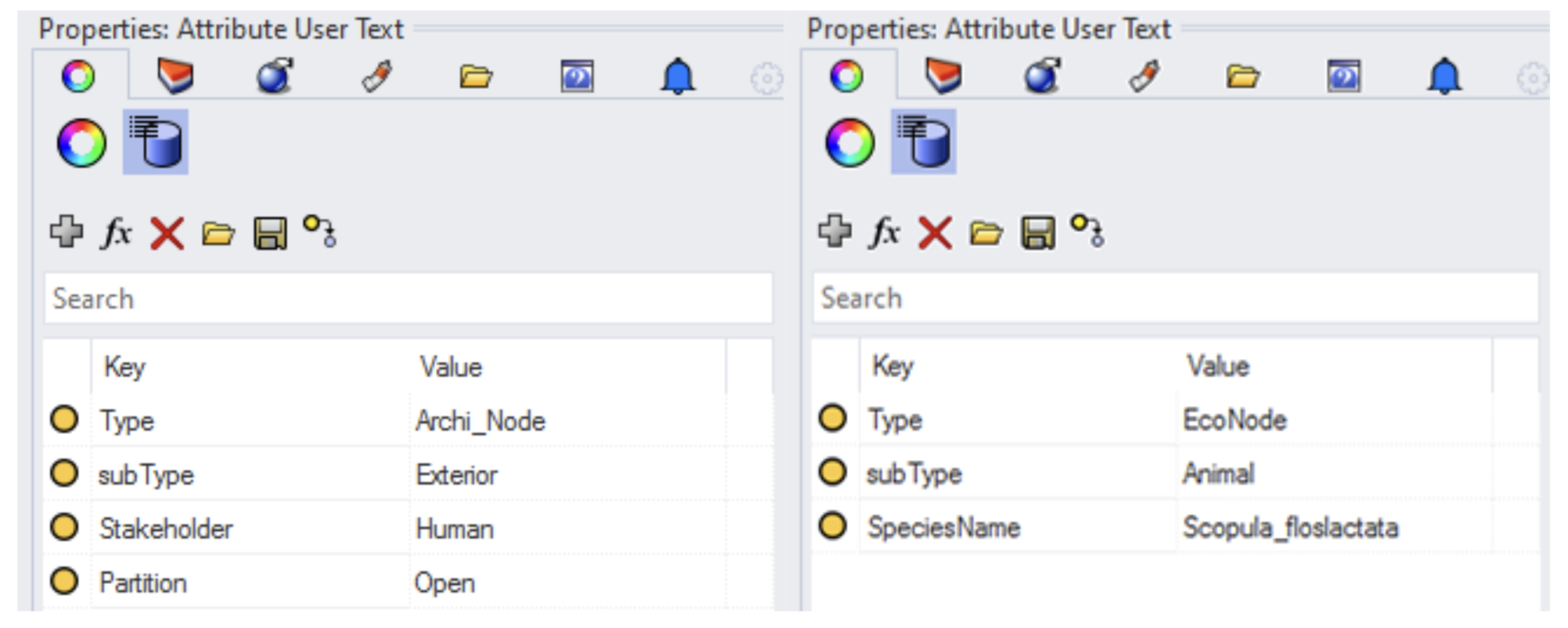
Figure 14.
The complete GH pipeline, which prepares points as JSON-LD, uploads them to GraphDB. Afterwards, validates the chosen constraints and returns a boolean value.
Figure 14.
The complete GH pipeline, which prepares points as JSON-LD, uploads them to GraphDB. Afterwards, validates the chosen constraints and returns a boolean value.
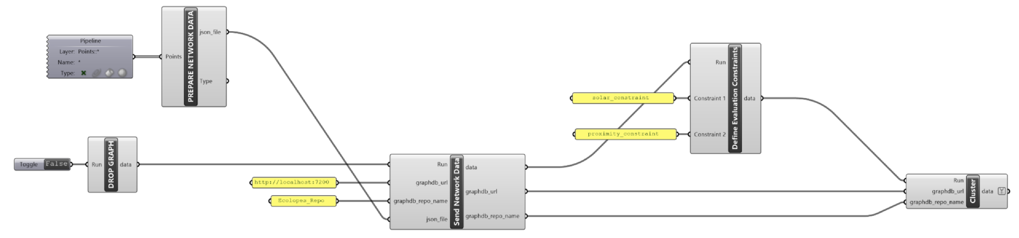
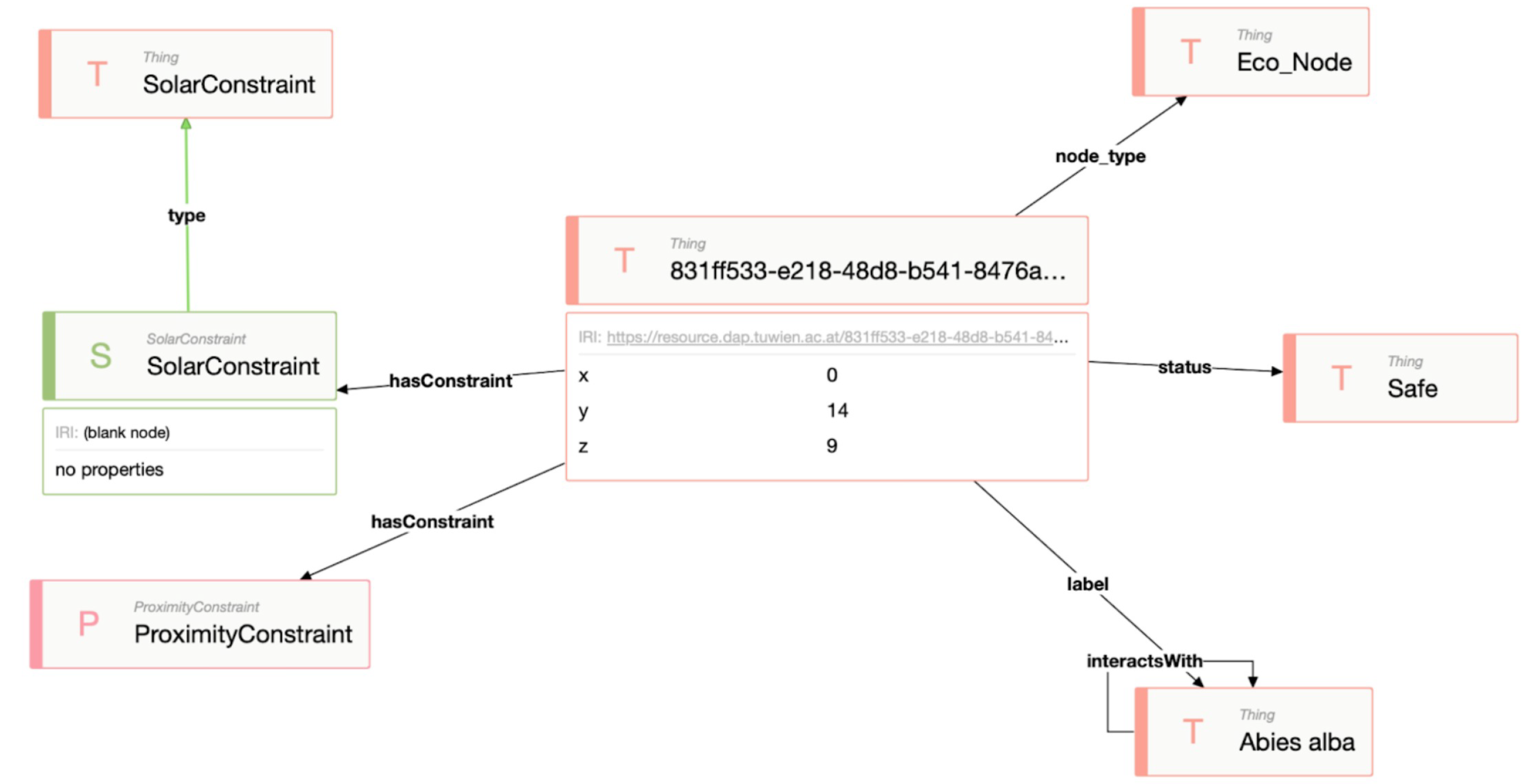
Figure 15.
The graph visualisation (in open access version of Ontodia [44]) of the EcoNode that satisfies both solar and proximity constraints.
Figure 15.
The graph visualisation (in open access version of Ontodia [44]) of the EcoNode that satisfies both solar and proximity constraints.
7. Conclusion and Future Work
This paper presented an ontology-driven approach to integrate diverse datasets from public APIs, private sources, and CAD environments into a unified RDF-based knowledge graph, facilitating ecological building design. By leveraging OBDM, the approach balances virtualization and materialization, ensuring efficient data integration while supporting advanced queries and reasoning. The ECOLOPES ontologies bridges life sciences and geometric data, enabling designers to address ecological constraints like solar radiation and proximity through interactive workflows. A case study highlighted the ontology’s practical application in designing habitats that promote species attractiveness and urban biodiversity. For future work, we plan to use SHACL to define constraints, use a rule language instead of SPARQL queries in order to adhere to Semantic Web standards. More importantly to extend the problem setting towards generative process (geometric articulation) of the ontology-aided generative computational design by employing more sophisticated approaches akin to answer set programming [45,46].
Acknowledgments
This work is funded by the European Union Horizon 2020 Future and Emerging Technologies research project ECOLOPES: ECOlogical building enveLOPES (grant number: 964414). The funding source is not involved in the conduct of the research or preparation of the article. Furthermore, we extend our gratitude to Mariasole Calbi for kindly providing the PFGs dataset, and to Victoria Culshaw for sharing the AFGs dataset. We thank Navid Javan for his work and assisting us with the Grasshopper workflow and components.
Conflicts of Interest
The authors declare no conflicts of interest. The funders had no role in the design of the study; in the collection, analyses, or interpretation of data; in the writing of the manuscript; or in the decision to publish the results.
Abbreviations
The following abbreviations are used in this manuscript:
| ABox | Assertion Box |
| AECO | Architecture, Engineering, and Construction |
| AFG | Animal Functional Group |
| API | Application Programming Interface |
| CAD | Computer Aided Design |
| CSV | Comma-Separated Values |
| CQs | Competency Questions |
| CRUD | Create, Read, Update and Delete |
| CWA | Closed World Assumption |
| ECOLOPES | ECOlogical building enveLOPES |
| EIM | Ecolopes Information Model |
| IFC | Industry Foundation Classes |
| IUCN | International Union for Conservation of Nature |
| FAIR | Findable, Accessible, Interoperable and Reusable |
| FET | Future and Emerging Technologies |
| HSI | Habitat Suitability Index |
| LOD | Linked Open Data |
| GBIF | Global Biodiversity Information Facility |
| GLoBI | Global Biotic Interactions |
| JSON | JavaScript Object Notation |
| JSON-LD | JavaScript Object Notation-Linked Data |
| KG | Knowledge Graph |
| KPI | Key Performance Indicator |
| MDPI | Multidisciplinary Digital Publishing Institute |
| RDF | Resource Description Framework |
| RDFS | Resource Description Framework Schema |
| OBDA | Ontology-based Data Access |
| OBDM | Ontology-based Data Management |
| OBO | Open Biological and Biomedical |
| OWA | Open World Assumption |
| OWL | Web Ontology Language |
| Portable Document Format | |
| PFG | Plant Functional Group |
| RML | RDF Mapping Language |
| SHACL | Shapes Constraint Language |
| SPARQL | SPARQL Protocol and RDF Query Language |
| SQL | Structured Query Language |
| TBox | Terminology Box |
| URI | Uniform Resource Identifier |
| UUID | Universally unique identifier |
| 1 | |
| 2 | |
| 3 | |
| 4 | |
| 5 | |
| 6 | Herein, we also distinguish taxonomies or controlled vocabularies as a part of KG, sometimes referred as CBox. They are essential to capture hierarchical representations, e.g., species taxonomic rank. |
| 7 | |
| 8 | |
| 9 | |
| 10 | |
| 11 | |
| 12 | Provided by city of Vienna https://www.wien.gv.at/umweltschutz/umweltgut/
|
| 13 | |
| 14 | |
| 15 | |
| 16 | We mention [43] as an approach that tackles canonical IRIs in the setting of virtual mappings and OBDM, while in our case this part of the data is materialised. |
| 17 | Alternatively, the latter can be computed via query rewriting during query time by using path queries in SPARQL owl:sameAs*. |
| 18 | |
| 19 |
References
- Perini, K.; Canepa, M.; Barath, S.; Hensel, M.; Mimet, A.; Uthaya Selvan, S.; Roccotiello, E.; Selami, T.; Sunguroglu Hensel, D.; Tyc, J.; et al. ECOLOPES: A multi-species design approach to building envelope design for regenerative urban ecosystems. 2021, 11. [Google Scholar]
- Lenzerini, M. Ontology-based data management. In Proceedings of the Proceedings of the 20th ACM International Conference on Information and Knowledge Management, CIKM ’11. New York, NY, USA, 2011; pp. 5–6. [Google Scholar] [CrossRef]
- Hensel, M. Performance-Oriented Architecture: Rethinking Architectural Design and the Built Environment, 1 ed.; Wiley, 2013. [CrossRef]
- Hensel, M.U.; Sunguroğlu Hensel, D. Performances of Architectures and Environments: En Route to a Theory and Framework. In The Routledge Companion to Paradigms of Performativity in Design and Architecture; Routledge, 2019. Num Pages: 12.
- Sunguroğlu Hensel, D.; Tyc, J.; Hensel, M. Data-driven design for Architecture and Environment Integration: Convergence of data-integrated workflows for understanding and designing environments. SPOOL 2022, 9, 19–34. [Google Scholar] [CrossRef]
- Poelen, J.H.; Simons, J.D.; Mungall, C.J. Global biotic interactions: An open infrastructure to share and analyze species-interaction datasets. Ecol. Inform. 2014, 24, 148–159. [Google Scholar] [CrossRef]
- Calbi, M.; Boenisch, G.; Boulangeat, I.; Bunker, D.; Catford, J.A.; Changenet, A.; Culshaw, V.; Dias, A.S.; Hauck, T.; Joschinski, J.; et al. A novel framework to generate plant functional groups for ecological modelling. Ecol. Indic. 2024, 166, 112370. [Google Scholar] [CrossRef]
- Tyc, J.; Selami, T.; Hensel, D.S.; Hensel, M. A Scoping Review of Voxel-Model Applications to Enable Multi-Domain Data Integration in Architectural Design and Urban Planning. Architecture 2023, 3, 137–174. [Google Scholar] [CrossRef]
- Fensel, D.; Şimşek, U.; Angele, K.; Huaman, E.; Kärle, E.; Panasiuk, O.; Toma, I.; Umbrich, J.; Wahler, A. Knowledge graphs: Methodology, tools and selected use cases, 1 ed.; Springer Nature: Cham, Switzerland, 2020. [Google Scholar]
- Hogan, A.; Blomqvist, E.; Cochez, M.; d’Amato, C.; de Melo, G.; Gutiérrez, C.; Kirrane, S.; Gayo, J.E.L.; Navigli, R.; Neumaier, S.; et al. Knowledge graphs [J]. Synthesis Lectures on Data Semantics and Knowledge 2021. [Google Scholar]
- Poggi, A.; Lembo, D.; Calvanese, D.; Giacomo, G.D.; Lenzerini, M.; Rosati, R. Linking Data to Ontologies. J. Data Semant. 2008, 10, 133–173. [Google Scholar]
- Ahmeti, A. Updates in the context of ontology-based data management. PhD thesis, Technische Universität Wien, Wien, 2020. [CrossRef]
- Sequeda, J.F.; Arenas, M.; Miranker, D.P. OBDA: Query rewriting or materialization. In practice, both! In The Semantic Web – ISWC 2014; Lecture notes in computer science, Springer International Publishing: Cham, 2014; pp. 535–551. [Google Scholar]
- Grüninger, M.; Fox, M.S. Methodology for the design and evaluation of ontologies. In Proceedings of the IJCAI95 Workshop on Basic Ontological Issues in Knowledge Sharing, Montreal; 1995. [Google Scholar]
- Smith, B.; Ceusters, W.; Klagges, B.; Köhler, J.; Kumar, A.; Lomax, J.; Mungall, C.; Neuhaus, F.; Rector, A.L.; Rosse, C. Relations in biomedical ontologies. Genome Biol. 2005, 6, R46. [Google Scholar] [CrossRef]
- Glick, J. Ontologies and Databases – Knowledge Engineering for Materials Informatics. In Informatics for Materials Science and Engineering; Elsevier, 2013; pp. 147–187.
- Pruski, C.; Hensel, D.S. The Role of Information Modelling and Computational Ontologies to Support the Design, Planning and Management of Urban Environments: Current Status and Future Challenges. In Informed Urban Environments: Data-Integrated Design for Human and Ecology-Centred Perspectives; Chokhachian, A., Hensel, M.U., Perini, K., Eds.; Springer International Publishing: Cham, 2022; pp. 51–70. [Google Scholar]
- Polleres, A. From SPARQL to rules (and back). In Proceedings of the Proceedings of the 16th international conference on World Wide Web, New York, NY, USA; 2007. [Google Scholar]
- Muñoz, S.; Pérez, J.; Gutierrez, C. Minimal Deductive Systems for RDF. In Proceedings of the The Semantic Web: Research and Applications; Franconi, E.; Kifer, M.; May, W., Eds., Berlin, Heidelberg; 2007; pp. 53–67. [Google Scholar]
- Lenzerini, M. Data integration: a theoretical perspective. In Proceedings of the Proceedings of the Twenty-First ACM SIGMOD-SIGACT-SIGART Symposium on Principles of Database Systems, New York, NY, USA, 2002. [CrossRef]
- Srihari, S.N. Representation of Three-Dimensional Digital Images. ACM Computing Surveys 1981, 13, 399–424. [Google Scholar] [CrossRef]
- Tyc, J.; Sunguroğlu Hensel, D.; Parisi, E.I.; Tucci, G.; Hensel, M.U. Integration of Remote Sensing Data into a Composite Voxel Model for Environmental Performance Analysis of Terraced Vineyards in Tuscany, Italy. Remote Sensing 2021, 13, 3483. [Google Scholar] [CrossRef]
- Tyc, J.; Parisi, E.I.; Tucci, G.; Sunguroğlu Hensel, D.; Hensel, M.U. A data-integrated and performance-oriented parametric design process for terraced vineyards. Journal of Digital Landscape Architecture. [CrossRef]
- Ludwig, F.; Hensel, M.; Rötzer, T.; Ahmeti, A.; Chen, X.; Erdal, H.I.; Reischel, A.; Qiguan, S.; Tyc, J.; Yazdi, H. Digital Workflow for Novel Urban Green System Design Derived from a Historical Role Model. Journal of Digital Landscape Architecture (JoDLA) 2024, 2024, 333–345. [Google Scholar] [CrossRef]
- Hensel, M.U.; Tyc, J.M.; Hensel, D.S.; Ahmeti, A.; Cifci, M.A. ECOLOPES Voxel Model. Technical report, 2023.
- Dimou, A.; Sande, M.V.; Colpaert, P.; Verborgh, R.; Mannens, E.; de Walle, R.V. RML: A Generic Language for Integrated RDF Mappings of Heterogeneous Data. In Proceedings of the Proceedings of the Workshop on Linked Data on the Web co-located with the 23rd International World Wide Web Conference (WWW 2014), Seoul, Korea, April 8, 2014.
- Torta, G.; Ardissono, L.; La Riccia, L.; Savoca, A.; Voghera, A. Representing ecological network specifications with semantic web techniques. In Proceedings of the Proceedings of the 9th International Joint Conference on Knowledge Discovery, Knowledge Engineering and Knowledge Management.
- Sadeghineko, F.; Kumar, B. Application of semantic Web ontologies for the improvement of information exchange in existing buildings. Construction Innovation 2022, 22, 444–464. [Google Scholar] [CrossRef]
- Abanda, F.H.; Kamsu-Foguem, B.; Tah, J.H.M. BIM–New rules of measurement ontology for construction cost estimation. Engineering Science and Technology, an International Journal 2017, 20, 443–459. [Google Scholar] [CrossRef]
- Liao, L.; Wen, Y.; Mo, W.; Gan, C. A Carbon Footprint Management Framework for Prefabricated Buildings Based on Knowledge Graph. In Proceedings of the International Symposium on Advancement of Construction Management and Real Estate. Springer; 2023; pp. 1551–1569. [Google Scholar]
- Olanrewaju, O.I.; Enegbuma, W.I.; Donn, M.; Chileshe, N. Building information modelling and green building certification systems: A systematic literature review and gap spotting. Sustainable Cities and Society 2022, 81, 103865. [Google Scholar] [CrossRef]
- Shi, J.; Pan, Z.; Jiang, L.; Zhai, X. An ontology-based methodology to establish city information model of digital twin city by merging BIM, GIS and IoT. Advanced Engineering Informatics 2023, 57, 102114. [Google Scholar] [CrossRef]
- Sica, F.; De Paola, P.; Tajani, F.; Doko, E. Spatial–Temporal Ontology of Indicators for Urban Landscapes. Land 2025, 14, 72. [Google Scholar] [CrossRef]
- Affinito, F.; Holzer, J.M.; Fortin, M.J.; Gonzalez, A. Towards a unified ontology for monitoring ecosystem services 2024.
- Ma, R.; Li, Q.; Zhang, B.; Huang, H.; Yang, C. An ontology-driven method for urban building energy modeling. Sustainable Cities and Society 2024, 106, 105394. [Google Scholar] [CrossRef]
- Al-Ageili, M.; Mouhoub, M. An ontology-based information extraction system for residential land-use suitability analysis. International Journal of Software Engineering and Knowledge Engineering 2022, 32, 1019–1042. [Google Scholar] [CrossRef]
- Hu, X.; Chen, Q.; Du, M. Ontology-based multi-sensor information integration model for urban gardens and green spaces. In Proceedings of the IOP Conference Series: Earth and Environmental Science. IOP Publishing, Vol. 615; 2020; p. 012023. [Google Scholar]
- Santos, H.; Dantas, V.; Furtado, V.; Pinheiro, P.; McGuinness, D.L. From data to city indicators: A knowledge graph for supporting automatic generation of dashboards. In Proceedings of the The Semantic Web: 14th International Conference, ESWC 2017, Portorož, Slovenia, 2017, Proceedings, Part II 14. Springer, 2017, May 28–June 1; pp. 94–108.
- Calvanese, D.; Cogrel, B.; Komla-Ebri, S.; Kontchakov, R.; Lanti, D.; Rezk, M.; Rodriguez-Muro, M.; Xiao, G. Ontop: Answering SPARQL queries over relational databases. Semant. Web 2017, 8, 471–487. [Google Scholar] [CrossRef]
- Penev, L.; Dimitrova, M.; Senderov, V.; Zhelezov, G.; Georgiev, T.; Stoev, P.; Simov, K. OpenBiodiv: A knowledge graph for literature-extracted linked open data in biodiversity science. Publications 2019, 7, 38. [Google Scholar] [CrossRef]
- Ahmeti, A.; Schakel, J.K.; David, R.; Revenko, A. Towards preserving Biodiversity using Nature FIRST Knowledge Graph with Crossovers. In Proceedings of the Proceedings of the ISWC 2023 Posters, Demos and Industry Tracks: From Novel Ideas to Industrial Practice co-located with 22nd International Semantic Web Conference (ISWC 2023), Athens, Greece, November 6-10, 2023.
- Kyzirakos, K.; Savva, D.; Vlachopoulos, I.; Vasileiou, A.; Karalis, N.; Koubarakis, M.; Manegold, S. GeoTriples: Transforming geospatial data into RDF graphs using R2RML and RML mappings. Journal of Web Semantics 2018, 52-53, 16–32. [Google Scholar] [CrossRef]
- Xiao, G.; Hovland, D.; Bilidas, D.; Rezk, M.; Giese, M.; Calvanese, D. Efficient ontology-based data integration with canonical IRIs. In The Semantic Web; Lecture notes in computer science, Springer International Publishing: Cham, 2018; pp. 697–713. [Google Scholar]
- Mouromtsev, D.; Pavlov, D.; Emelyanov, Y.; Morozov, A.; Razdyakonov, D.; Galkin, M. The Simple Web-based Tool for Visualization and Sharing of Semantic Data and Ontologies. In Proceedings of the International Semantic Web Conference (Posters & Demos); 10 2015. [Google Scholar]
- Eiter, T.; Ianni, G.; Krennwallner, T. Answer Set Programming: A Primer. In Reasoning Web. Semantic Technologies for Information Systems: 5th International Summer School 2009, Brixen-Bressanone, Italy, August 30 - September 4, 2009, Tutorial Lectures; Tessaris, S., Franconi, E., Eiter, T., Gutierrez, C., Handschuh, S., Rousset, M.C., Schmidt, R.A., Eds.; Springer Berlin Heidelberg: Berlin, Heidelberg, 2009; pp. 40–110. [Google Scholar]
- Erdem, E.; Gelfond, M.; Leone, N. Applications of answer set programming. AI Mag. 2016, 37, 53–68. [Google Scholar] [CrossRef]
Figure 1.
Three types of voxel data layers and their 3D visualisations provided by the current selection of temporal datasets [25].
Figure 1.
Three types of voxel data layers and their 3D visualisations provided by the current selection of temporal datasets [25].
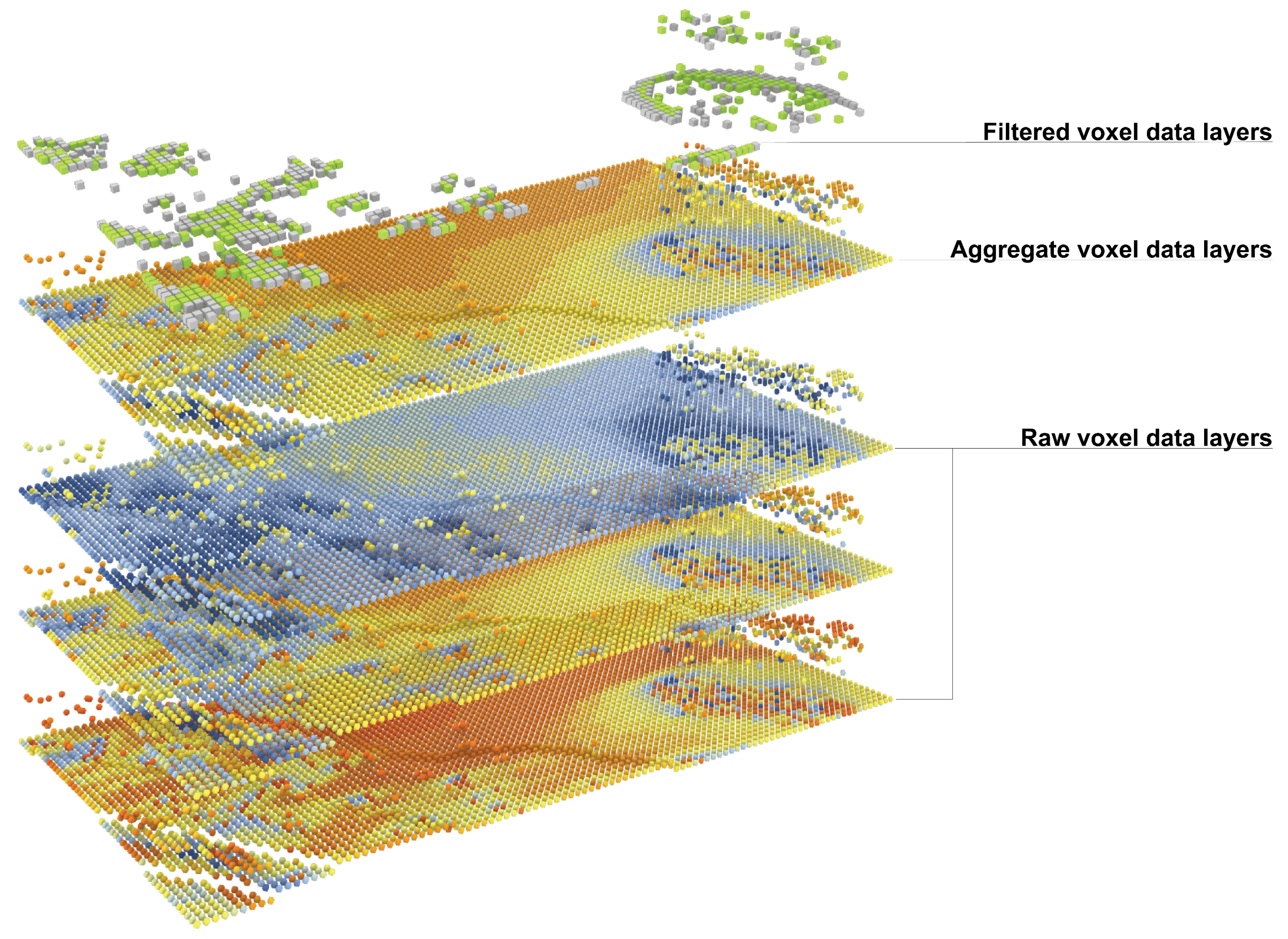
Figure 2.
Ontology-based data management - data integration framework of heterogeneous datasets. Some of the datasets are materialised in KG (RML [26] and Ontotext Refine mappings), with the aim of achieving better query or update performance; while voxel model containing data of high volume and not subject to frequent changes is virtualised.
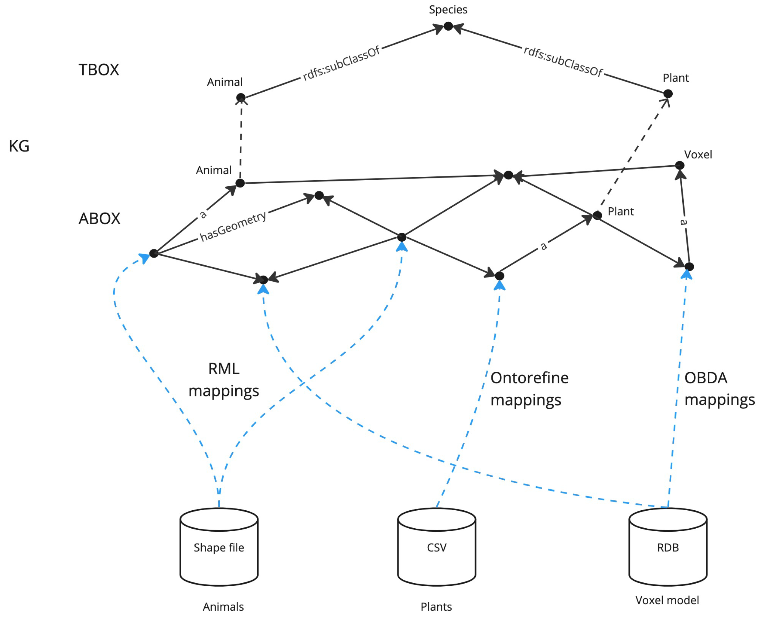
Figure 3.
The placement of Nodes in CAD environment and their validation against the knowledge graph. Nodes that fulfil the constraints are depicted as green circles, whereas the ones that do not are depicted as red crosses (left figure). In this case constraints are subject to proximity distance between nodes or/and solar radiation (yellow highlighted area), which has the information encoded in the voxel model, and therefore both can be queried via the knowledge graph. Grasshopper (right) is used as a component for doing the orchestration process of the validation.
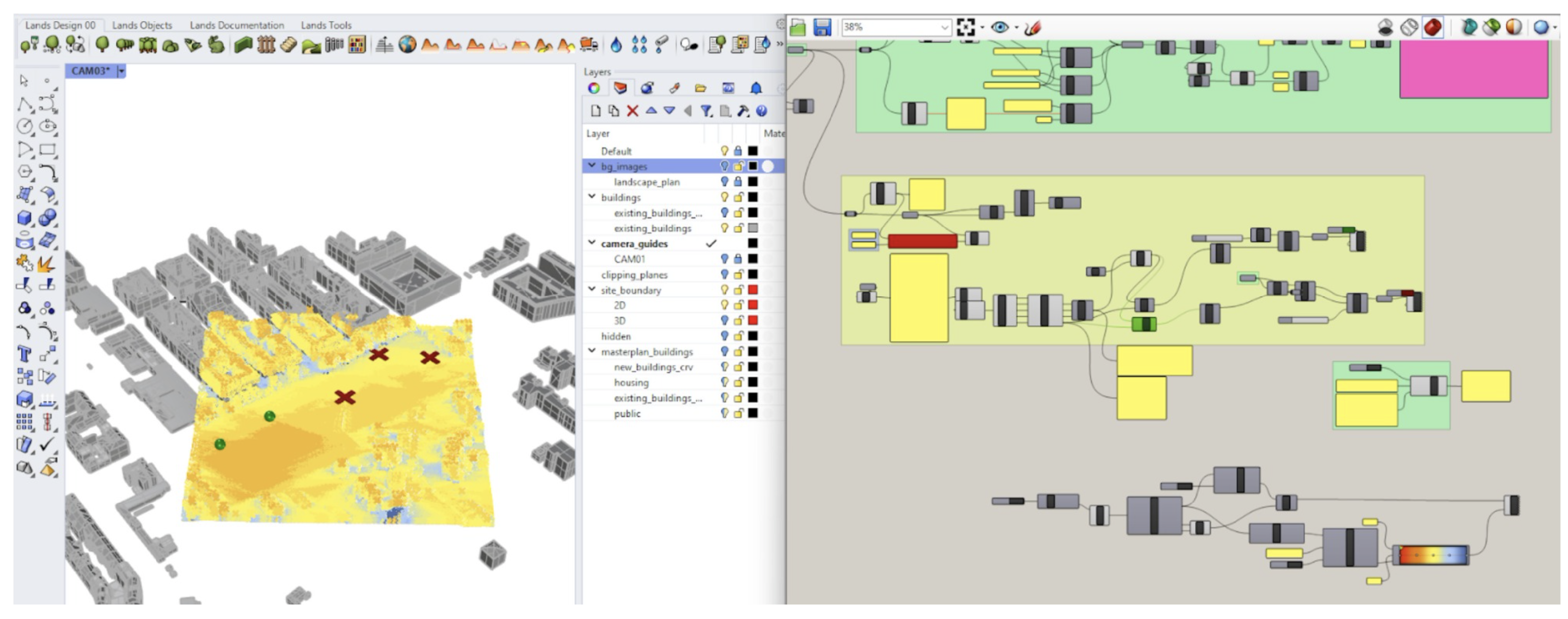
Figure 4.
OBO Relations alignment using owl:equivalentProperty relations stored in a separate named graph https://tbox.crossovers.dap.tuwien.ac.at.
Figure 4.
OBO Relations alignment using owl:equivalentProperty relations stored in a separate named graph https://tbox.crossovers.dap.tuwien.ac.at.
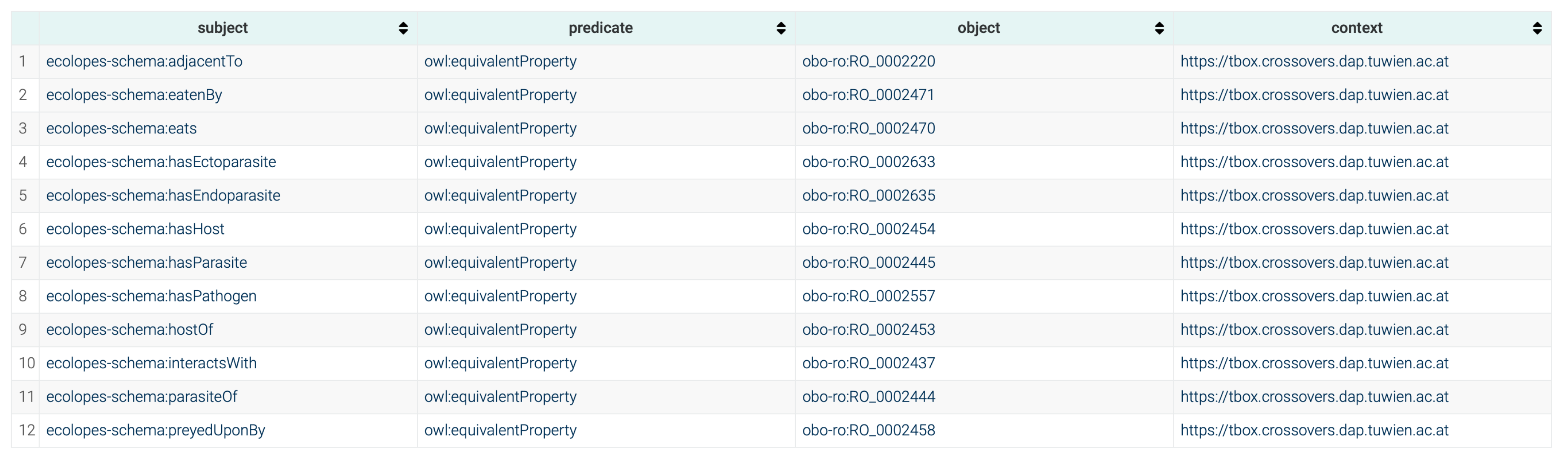
Figure 5.
Native OBDA mappings expressed in RDF Turtle syntax, which are used in the configuration of the GraphDB repository.
Figure 5.
Native OBDA mappings expressed in RDF Turtle syntax, which are used in the configuration of the GraphDB repository.
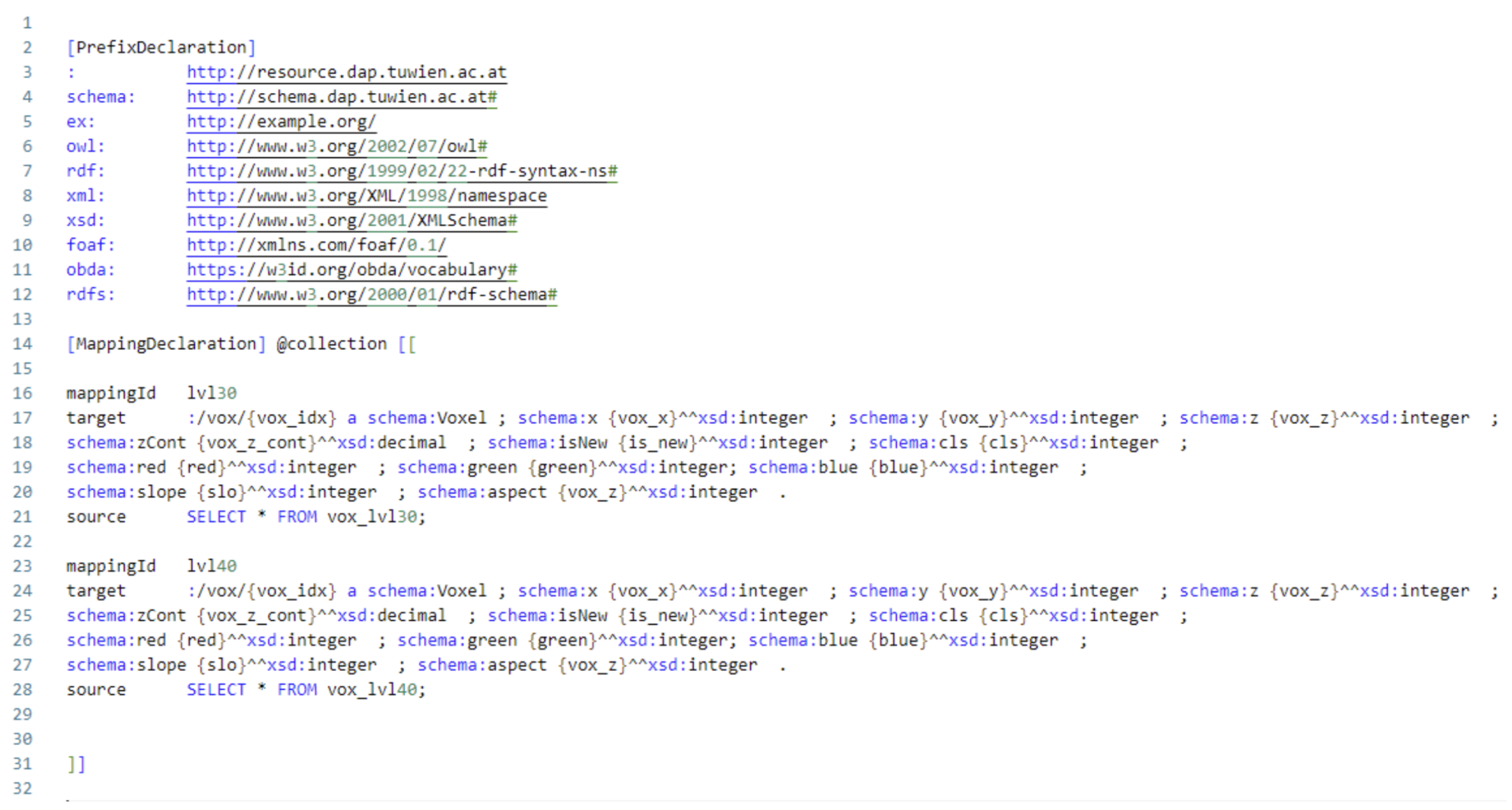
Figure 6.
SPARQL queries–subject to mappings (cf. Figure 5)–are translated on-the-fly to SQL queries, which are used to run against the Postgres RDB and the results are returned.
Figure 6.
SPARQL queries–subject to mappings (cf. Figure 5)–are translated on-the-fly to SQL queries, which are used to run against the Postgres RDB and the results are returned.
Figure 7.
Grasshopper pipelines pose the SPARQL queries that calculate the permissible positions where one can place a plant species based on plant’s solar requirements.
Figure 7.
Grasshopper pipelines pose the SPARQL queries that calculate the permissible positions where one can place a plant species based on plant’s solar requirements.
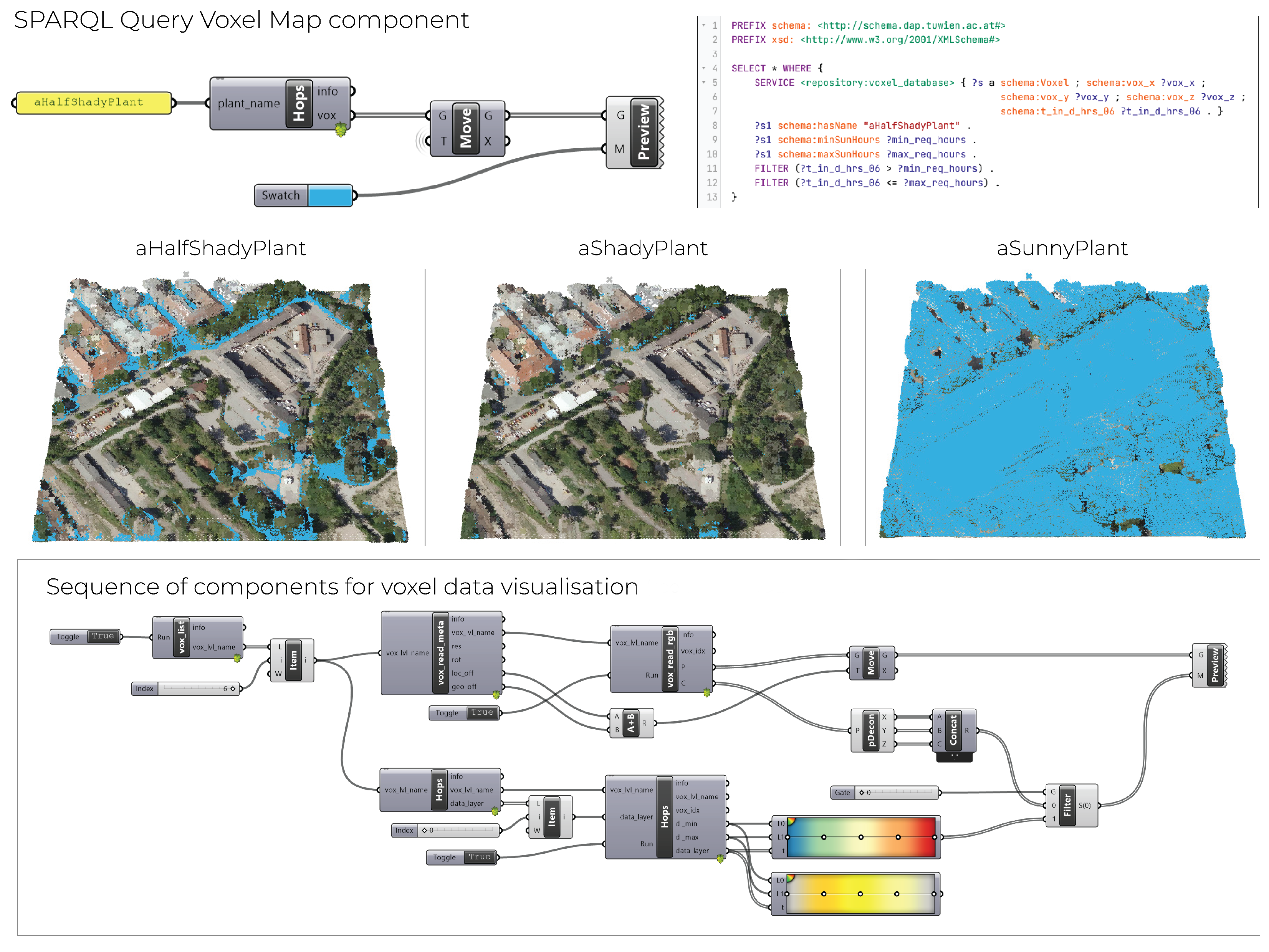
Figure 8.
Knowledge graph snapshot connecting data from different environments. The resulting graph data is managed in the GraphDB triple store. The dashed lines represent implicit equality between entities in KG (i.e., the relation need to be resolved via species latin name), whereas in other cases they are explicitly asserted using owl:sameAs relations.
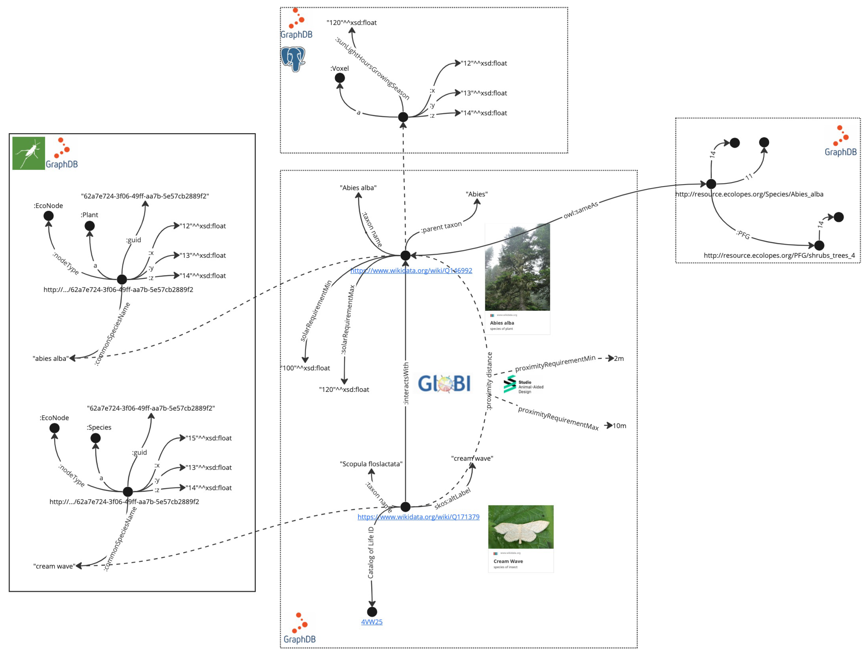
Figure 9.
Ontotext Refine mappings for mapping source and target species, as well as including the type of interaction between them. More metadata can be mapped on demand.
Figure 9.
Ontotext Refine mappings for mapping source and target species, as well as including the type of interaction between them. More metadata can be mapped on demand.
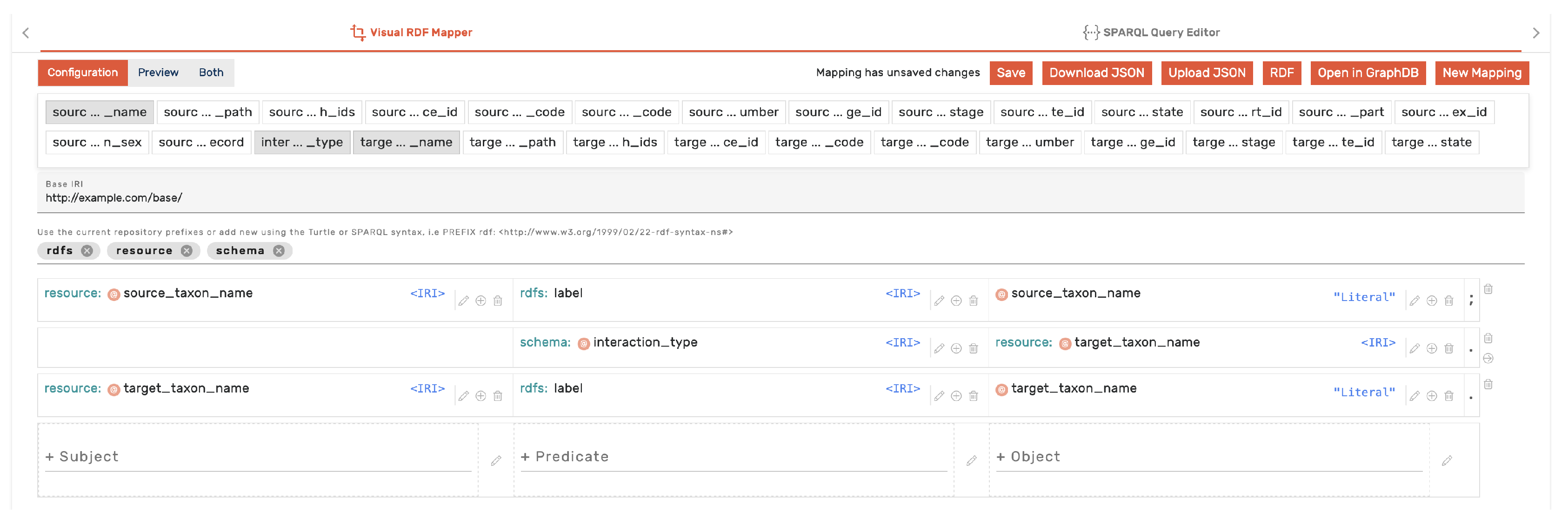
Figure 10.
Integrated data on the species Abies Alba from different datasets: GloBI (central), PFGs (metadata panel on the right) and CAD (UUID node) in GraphDB environment. Due to the limitation in the visualisation feature, RDF* data from Example 2 are not shown, despite that they exist in separate named graph and can be queried using SPARQL*.
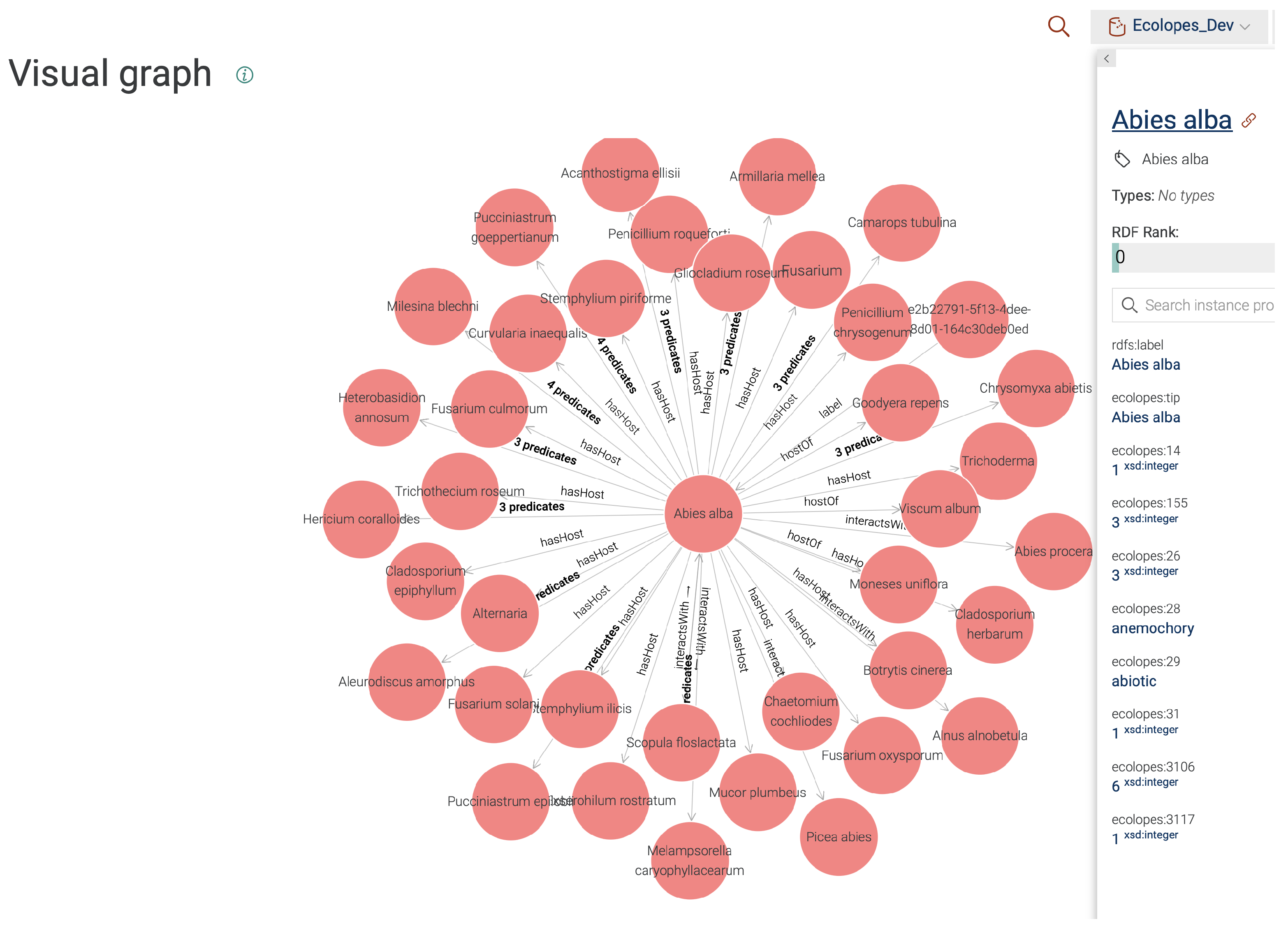
Figure 11.
The citizen science data on species obtained from GBIF in the proximity of Nordbahnof.
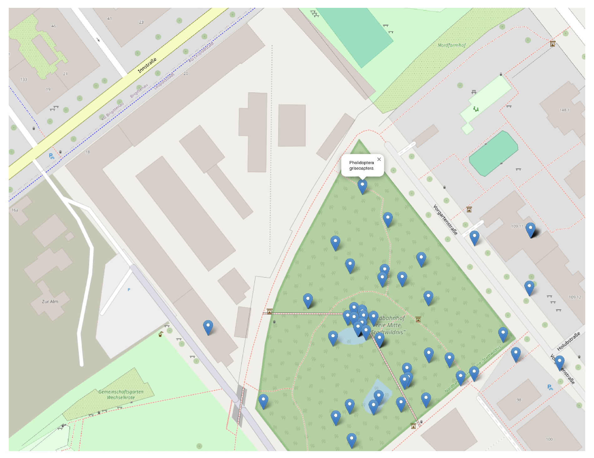
Figure 12.
INSERT query – as a counterpart to CONSTRUCT – that inserts the validation results based on the proximity constraints. INSERT queries are issued in the context of OBDM to mimic the rule-based approach.
Figure 12.
INSERT query – as a counterpart to CONSTRUCT – that inserts the validation results based on the proximity constraints. INSERT queries are issued in the context of OBDM to mimic the rule-based approach.
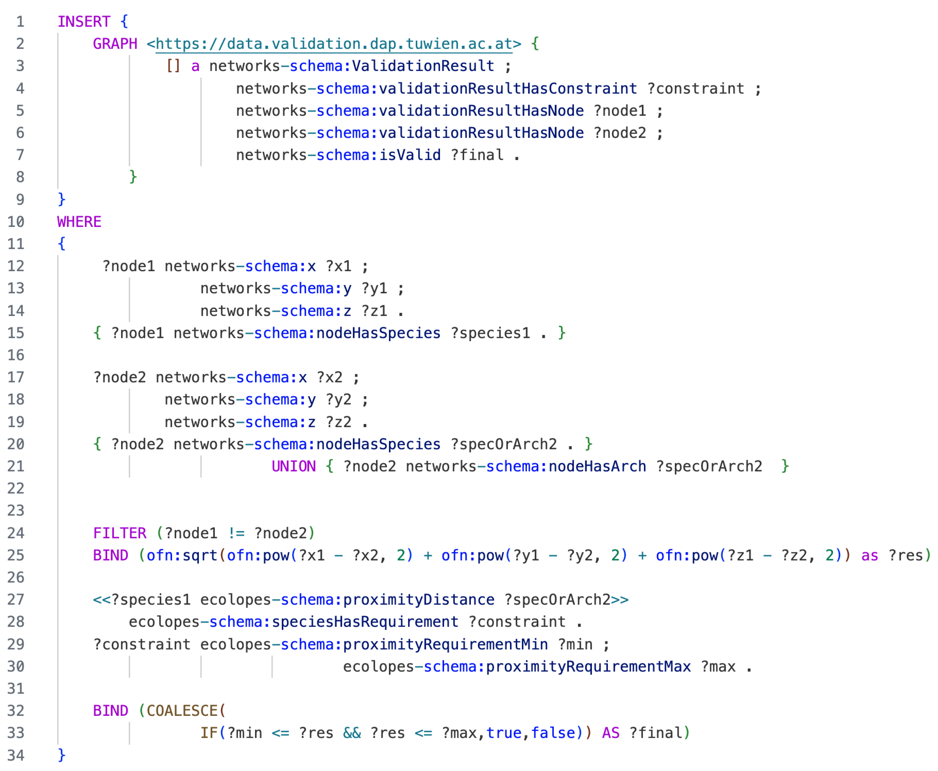
Table 2.
The datasets that are mapped and integrated into the Ecolopes KG.
| Dataset No. | Spatial | Input Format | Mapping language | Triple count |
|---|---|---|---|---|
| 1. | (x) | CSV | Ontotext Refine | 3548 |
| 2. | x | shapefile | RML | 881 |
| 3. | x | CSV | Ontotext Refine | 492* |
| 4. | (x) | CSV | Ontotext Refine | 2454463 |
| 5. | - | JSON | RML | 256 |
| 6. | (x) | - | 34** | |
| 7. | (x) | CSV | Ontotext Refine | 2858* |
| 8. | - | RDF | - | 136865946 |
| 9. | (x) | RDF | - | 3889978*** |
| 10. | (x) | RDF | - | 5363877 |
| 11. | x | - (CAD metadata) | Grasshopper components | 20**** |
| 12. | x | RDB | OBDA | 1329096 |
| (x) for spatial means partial/implicit coverage. | ||||
| *Triple count depends on the number of API requests. | ||||
| **Placeholder data. | ||||
| ***SELECT (COUNT(*) as ?cnt) WHERE ?item wdt:P225 ?taxon . | ||||
| ****Triples vary depending on the complexity and size of the CAD network. | ||||
Disclaimer/Publisher’s Note: The statements, opinions and data contained in all publications are solely those of the individual author(s) and contributor(s) and not of MDPI and/or the editor(s). MDPI and/or the editor(s) disclaim responsibility for any injury to people or property resulting from any ideas, methods, instructions or products referred to in the content. |
© 2025 by the authors. Licensee MDPI, Basel, Switzerland. This article is an open access article distributed under the terms and conditions of the Creative Commons Attribution (CC BY) license (http://creativecommons.org/licenses/by/4.0/).
Copyright: This open access article is published under a Creative Commons CC BY 4.0 license, which permit the free download, distribution, and reuse, provided that the author and preprint are cited in any reuse.


