Submitted:
23 February 2025
Posted:
25 February 2025
You are already at the latest version
Abstract
The δ-GLMB filter is an analytic solution to the multi-target Bayes recursion using in multi-target tracking. Theoretically, the δ-GLMB filter handles uncertainties in measurements in its filtering procedure. However, in practice, degeneration of the measurement quality affects the performance of this filter. In this paper, we will discuss the effects of increasing measurement uncertainty on δ-GLMB filter and also will propose two heuristic methods to improve the performance of the filter in such conditions. The base idea of proposed methods is to utilize the information stored in the history of the filtering procedure, which can be used to decrease the measurements uncertainty effects on the filter. Since the GLMB filters have shown good results in the field of multi-target tracking, an uncertain immune δ-GLMB can play as a strong tool for this area. In this study, the results indicate that the proposed heuristic ideas can improve the performance of the filtering in presence of uncertain observations.
Keywords:
Multi target tracking
; N-Scan δ-GLMB
; Refined δ-GLMB
; Measurement uncertainty effect reduction
1. Introduction
Multi-Target tracking (MTT) is the procedure of estimating a time-varying number of targets and their states from a sequence of observations. The number of targets are usually unknown and the observations are noisy due to uncertainty of detection and presence of spurious targets (clutter) [1,2,3,4,5]. The trajectory of a target is another important outcome of MTT, [6] proposes a Bayesian multi-target tracking solution that also provides estimates of target trajectories. MTT suffers from main challenges including detection uncertainty and clutter that mislead the tracker and cause efficiency reduction in estimating number of targets, their states and trajectories. However there are many approaches to MTT, three paradigms are discussed as the main solutions. These are, Multiple Hypotheses Tracking (MHT) [7,8,9], Joint Probabilistic Data Association (JPDA) [10,11,12], and Random Finite Set (RFS) [13,14,15,16]. Using RFS approach in MTT, provides a sophisticated Bayesian formulation for this problem in which a group of target states (multi-target states) are considered as a finite set [17,18]. This framework is a very popular method in estimating multi-target with applications in computer vision [19,20], robotics [21,22,23], sonar [24,25,26], monitoring and surveillance systems [27,28], sensor networks [29,30,31], cell biology [32,33], augmented reality [34,35], and etc. In RFS approach the density of multi-target states is propagated recursively forward in time using the Bayes multi-target filter [36]. The Bayes filter is a multi-target tracker, where target specifications are incorporated into individual state (as what occurs in RFS method, states of multi-target in a unit of time are incorporated in a single set). Since Bayes multi-target filter is intractable due to intense numerical complexity, the Probability Hypothesis Density (PHD) [37], Cardinalized PHD (CPHD) [38] and multi-Bernoulli filters [39] have been developed as approximations to the Bayes filter. In this work, we concentrate on an analytic solution to the Bayes MTT, known as the -Generalized Labeled Multi-Bernoulli (-GLMB), which uses RFS notion to behave targets as distinguishable and unique entities. This filter is applicable of keeping trajectories and it includes conjugate priors, which are closed under Chapman-Kolmogrov equation. However, results in [40,41,42] show promising performance in this filter, the performance of the filter decreases in situations that observation quality drops. The aim of this paper is to reduce effect of low detection rate and existence of clutter on the -GLMB filtering procedure. Consequent to the mentioned weakness, in particular we propose two methods, N-scan -GLMB and Refined -GLMB to alleviate the uncertainties in the observations using the information that are extracted from history of filtering during the time, which we believe to contain useful information in order to decrease uncertainties. The key innovation is to detect the components which are considered for truncation in the filtering procedure, however their truncation may cause targets get lost in a low detection rate. Detecting such situation is verified from the aspect of considering filtering history during the running time. The keyword N-scan is adopted from [43] which is utilised in order to induce the concept of using history of information in a certain window with size N.
This paper is organized as follows. A brief overview of RFS, Bayesian multi-target filtering and GLMB filter is provided in Sec:Background. In sec:prop, N-scan -GLMB and refined -GLMB are introduced and discussed. Results of numerical examples are discussed in Sec:Results and concluding remarks and extensions are discussed in Sec:Conclusion.
2. Background
This section explains summary of the labeled RFS formulation of the MTT and the -GLMB filter proposed in [41] with implementation details in [40].
In this paper, the standard inner product notation is shown as . Considering h as a real valued function then the notation of multi-object exponential is shown as where by convention. For a given set X, the cardinality (element numbers of that set) is denoted by . The generalisation of the Kroneker delta is denoted by
where the the input argument may be in any arbitrary form such as vectors, sets, etc. A generalisation of the indicator function, by
In this paper single target states are represented by lowercase letter e.g. x, Multi-target states are represented by uppercase letter e.g. X, Spaces are represented by blackboard bold e.g. .
2.1. Labelled Random Finite Sets
The RFS is a random variable finite set which includes random number of unordered points [14]. Since the number of points is random it is possible to consider a cardinality distribution for the RFS. The collection of target states is treated as a RFS with a certain cardinality distribution which enables MTT process without knowing the number of targets in the system. Labelled RFS is an extension to RFS notion which tries to keep the track of each target identity. For this purpose each target state is augmented with a unique unobserved label drawn from a discrete countable space , where ’s are distinct and denotes a positive integer set.
2.1.1. Bernoulli RFS
The probability density of a Bernoulli RFS X on is denoted by [44]
where r is the probability that the RFS have only one element and is the probability that the RFS is empty. The element inside the RFS (in case of existence) is distributed according to probability density . It is also remarkable that a Bernoulli RFS cardinality distribution is a Bernoulli distribution with parameter r.
2.1.2. Multi-Bernoulli RFS
A Multi-Bernoulli RFS X consists of union of multiple independent Bernoulli RFS with existence probability , which , i.e., . is a probability density defined on . In [41] Multi-Bernoulli RFS is denoted by following alternative form which is abbreviated .
2.1.3. Labelled Multi-Bernoulli RFS
In [41] there is a derivation shows that the following formulation is alternative form of the LMB mentioned in Appendix:prob
where denotes the distinct label indicator and is a function defined on and a projection , hence is the X labels set. The parameter is defined as following [41]
It is remarkable that a labelled RFS and its unlabelled version have the same cardinality distribution [41], proposition 2.
2.2. Generalised Labelled Multi-Bernoulli RFS
Generalised Labelled Multi-Bernoulli (GLMB) RFS is a family of labelled RFS distributions. GLMB is closed under the multi-object Chapman-Kolmogorov equation with respect to the multi-object transition kernel [41]. The probability density of a GLMB RFS X on is denoted by
where is a discrete index set, the weight term (Non-negative weights) and the exponential term satisfy the following conditions
A GLMB family can be explicated as a mixture of multi-target exponentials which its points are not statistically independent. The GLMB cardinality distribution is also given by
where presents the collection of finite subsets of with exactly n elements (if no subscript n exists in the definition then there is no restriction on number of elements).
2.3. Bayesian multi-target filtering
MTT system is used to jointly estimate the number of targets and their states from the measured observations. Due to dynamic nature of the MTT problem, births, spawn and death of targets, the number of targets is a changing variable over time. In MTT the targets and observations are considered as random finite sets which is defined respectively as , , where k is the indicator of time, is the number of targets in multi-target RFS at time k and is the number of observations at time k. Some observations in may be a clutter and some may be missed according to a underlying probability density function. is the multi-target likelihood function at time k which encapsulates the underlying models for clutter and detection. is the multi-target transition density at time k which encapsulates the underlying models of births, spawns, deaths and target motions. The multi-target Bayes filter propagates in time [44] according to the following update and prediction
where the integral is a set integral and presents the multi-target filtering density at time k.
2.4. Measurement Likelihood Function
The multi-object observation set is a union of detected states and clutters. Each state is either detected with probability or missed with . If the state is detected, it generates an observation point z with likelihood function . Considering independent detection conditioned on X and independent clutter from detection points with a Poisson distribution with intensity function the multi-object likelihood function is denoted by
where
2.5. Delta-Generalized Labeled Multi-Bernoulli
Delta-Generalized Labeled Multi-Bernoulli (-GLMB) is an analytic solution to the Bayes multi-target filter which is a member of GLMB family. Despite the closeness of this family under Chapman-Kolmogrov equation (hence, closed under the Bayes recursion), the numerical implementation of such family is ambiguous. In order to solve this problem, there is an alternative form for GLMB known as -GLMB which is denoted by
Substitution the term with in GLMB is a new presentation that simplifies the numerical implementation [40].
The -GLMB filter and specially the prediction operation, is conditioned on measurements observed up to time k. The discrete space contains the association map histories from the initial point of filtering history up to present time of filtering [40]. Let shows the association map space at time t, then can be defined as . Hence the update and prediction densities of a -GLMB is denoted as following, respectively
where , is a association history map up to time k. It is noticeable that the history association map contains every target label during the time, births, deaths and spawned targets. considering as a representation of a track label at time k, the pair is known as hypothesis. The weight of a hypothesis is the probability of the corresponding weight. is the density of the kinematic state of track ℓ for each .
For propagating the densities forward in time Bayesian recursion is used. As shown in [40] the results are closed form solutions for updating and prediction. The update formula of a -GLMB is denoted by
where denotes association maps which are related to components with identity domain I,
And the prediction formula is denoted by
where (considering S as a survival component indicator and B as newly born ones, ⊇ is sign for super set concept and subscript + is used for time )
-GLMB performs filtering via a recursion which propagates the multi-target filtering density forward in time [40] each iteration consist of a prediction, update and state extraction which estimates the target states from the filtering density.
2.6. N-Scan GM-PHD filter
GM-PHD filter has been proposed by [45] as a closed-form solution to the PHD filter [37]. The GM-PHD filter models each target with a Gaussian component with an associated weight (), mean () and covariance (). After performing predict and update phase, this filter extracts the Gaussian components whose weights are greater than a predefined threshold to estimate the multi-target states at each step and discard those components recon as non-informative, due to the value of their weights [45]. This pruning method is not always effective, suppose that the measurement of the target is uncertain hence, the weight of the target is significantly decreased and the estimation of the target is lost. [43] proposes a N-scan approach which improves the performance of the GM-PHD filter. This method benefits from the N last history of the targets to prevent missing the estimation of the targets in different uncertainties. N-Scan GM-PHD defines each Gaussian component with extra parameters including and in order to improve the tracking performance of the GM-PHD method, where is a binary confidence indicator showing a component is extracted before or not and is a weight history for component i containing the N last weights of the component, . N-Scan GM-PHD filter propagates parameter set in time and utilise these parameters in state extraction section in order to propose a new method for pruning, instead of discarding components compared with a predefined threshold. It calculates the number of weights which exceed the predefined threshold and treat them with a new pruning policy which considers the whole N sized history window of weights (More details are available in [43]). Experiment results in [43] shows that considering the history of weights instead of a single weight at a moment k, improves immunity of the filtering procedure to the uncertainties occurring in the measurement.
3. Proposed Methods
Each iteration of -GLMB filter involves a prediction operation followed by an update operation. These operations generate multi-target exponential weighted sums [40] which the terms number are intractable due to super-exponential growth of the terms in time. It is not rational to exhaustively consider all the terms in computations, hence it is obligatory to prune some terms. Multi-object densities are truncated by keeping the most informative terms respect to their weights and discarding those reckon non-informative respect to their insignificant weights (the components with a weight lower than a predefined threshold are truncated). This section analyses truncation in uncertain conditions and shows that pruning phase of -GLMB causes some terms to be truncated from the filtering procedure which are informative during a time window, however their weights have decreased at the moment due to an uncertainty conditions like miss-detection.
As a sequel to [46] which proposed concept of N-scan -GLMB, this section details the N-scan -GLMB implementation and presents enhanced update and prediction phase regarding N-Scan concept.
3.1. Uncertainty Effects on -GLMB
In -GLMB filtering procedure, the pruning phase might cause a weak performance in scenarios with high uncertainty level (e.g. low detection probability, high clutter ratio, etc.). Suppose that one or more targets are not detected, due to miss-detection of these targets, their associated hypotheses weight () diminish hence the associated hypotheses of true tracks are removed from the filtering procedure and cause the filtering performance drops. Furthermore, from a mathematical point of view as it is obvious in eq:psi the low detection rate cause the parameter to decrease and as the result, the multi-state target density decreases. In such conditions losing true tracks produces a less informative approximation to the posterior distribution in eq:glmbupdate which is clearly obvious inferred from eq:eta, eq:glmbweight and eq:updateglmb.
3.2. N-Scan -GLMB
In -GLMB filtering procedure there is a pruning operation that discards the hypotheses whose weights are lower than an empirical predefined threshold .
where is defined as the pool of containing all hypotheses after pruning. All the hypotheses which exist in this pool continue in the filtering procedure and those which do not exist any more, are discarded. As mentioned before this operation takes occur in order to prevent increasing hypotheses numbers exponentially during the time and eventually make the filtering procedure intractable. This pruning and its sequel state extraction is not always effective as pointed out in Sec:Uncertainityeffect. Whenever the weight of a hypothesis degenerates below the threshold the hypothesis is discarded however, weight devaluation of a hypothesis may be a sequence of miss detection or another uncertainty.
In this paper, a simple and effective N-scan approach [43,46] is used for truncating the hypotheses instead of discarding those with weight lower than an empirical predefined threshold . Using N-scan approach improves the performance of the previous methods specially in scenarios with lower SNR ratio which reckon as uncertain conditions. The suggested method benefits from the N last history of the weights of hypotheses to struggle with possible uncertainties. A -GLMB is completely characterised by the set of parameters . This paper follows [40] which considers parameters set of -GLMB as an enumeration of all hypotheses together with their weights and track densities. This assumption aims ease of the implementation procedure. Considering the mentioned assumption the -GLMB parameters set are shown as where and . With respect to this presentation of parameters set the N-scan method adds two additional parameters and , therefore new parameters set is shown as following
where is the binary confidence indicator for all hypothesis in . It determines whether a hypotheses h is discarded in previous iterations or not. The value of for each hypothesis is initialised to zero at initiation of the hypotheses, whenever a hypothesis satisfies the extraction conditions, the value of is changed to one. is the weight history of each hypothesis which keeps the last N weights of a hypothesis h, i.e.
These extended version of parameters set is propagated during the filtering procedure. The additional parameters are utilised to improve the tracking performance of the -GLMB filter in more uncertain conditions. The overall steps of proposed N-scan -GLMB algorithm is summarised as follows.
3.2.1. Initialization
In the -GLMB filter, each hypothesis is initialised by a proper setting. Additional to that setting w.r.t new parameter set it is needed that and be initialised too. Since the newly born hypothesis has not been extracted before, the initial value for is zero. All first elements of is set to zero (no history is available before initialisation) and the element is set to the ordinary initialisation value of a hypothesis
where .
Note that the initialisation of a hypothesis may occur in the middle of filtering time due to new born targets or spawned targets. In this situation initialisation of and is the same as mentioned above.
3.2.2. Prediction
In the prediction step of the -GLMB filter the filtering density is estimated as explained in Sec:Delta-Gen. However the estimation of the filtering density in the N-scan method is not altered, the newly defined parameters which is used in further steps propagate during time. The following propagation schema is appended to the prediction step of the -GLMB filter
3.2.3. Update
In the update step of the -GLMB filter the filtering density is estimated by eq:glmbupdate. Additional to estimation of which is in presence of the observing measurements, the weight history of a hypothesis is updated too. The weight history updating procedure is denoted by
where stands for the element of vector WH. Intuitively, the update procedure of WH is equal to remove the first element of the vector WH (The oldest weight of hypothesis h) and add the current weight of the hypothesis h to the weight history. Note that the order in the weight history matters which is an indicator of how much old is a weight.
3.2.4. Pruning and Extraction
In -GLMB filtering recursion there is a pruning phase that intend to avoid exponential growth of system by discarding the hypothesis with insignificant weights. This paper benefits from new defined parameters and to alter the procedure of pruning. The N-scan version of -GLMB does not discard the hypotheses which their weights are lower than at iteration k because the degeneration of the hypotheses weight could be as the result of a miss-detection or another uncertainty in the observation. Similar to the idea in [43], utilising new parameters which are added to the hypothesis parameter set, this paper proposes a new discarding method which the results show outperforms the previous methods. N-scan method tends to extract the hypotheses which satisfy either one of the following conditions and prune others,
Condition 1: (i.e. the hypothesis h has not been extracted yet) and .
Condition 2: (i.e. the hypothesis h has been extracted already) and . where shows the number of weights in which exceed , shows predefined threshold for extraction of newly born hypothesis and is the threshold for surviving hypotheses.
Note that if the first condition is satisfied then the value of changes to one because the hypothesis h is now extracted. Alg:1 summarises the N-scan method.
| Algorithm 1:Summary of N-Scan pruning algorithm. |
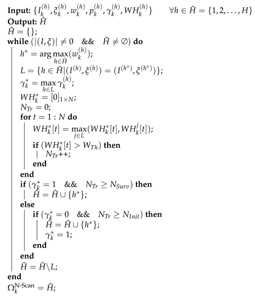 |
Intuitively, this method is proposed in order to give a second chance to hypotheses that are candidate for being discarded. Dependent on value of N this chance may increase relevantly. The idea behind giving a second chance to a hypothesis is to prevent truncation of informative hypotheses which belong to true target however, at the the moment k their observation is uncertain(e.g. due to miss-detection), hence its weight have dropped. However, using N-scan method for truncation the hypotheses add a slight burden on filtering procedure, it helps to reduce missing valuable information due to uncertainties. In the following the effect of N-scan on the filtering is pointed out in more detail.
Intuitively, N-scan method treats hypotheses with a weight lower than , in an optimistic way, it considers the reduction of their weight as a result of an uncertainty. In a window with size N which contains the weight history of the hypotheses, if the elements exceed at-least times, then the hypothesis extracts. Hence, the distribution of extraction is formulated as following form which is similar to a binomial trial
where is the probability that is greater than , this probability relates directly with i.e. (generally relates with uncertainty amount) and for surviving hypotheses and for newly born hypotheses.
However, with reduction of the falls too at the step k, the other terms which are saved inside the are able to increase , hence the miss-detection or generally any reason that makes degenerate, can be ignored for a restricted time period (relative with size of ). According to , increasing the value of N makes the filtering procedure more immune to uncertainty in exchange for keeping more hypotheses which complicates the system computations.
From another point of view N-scan provides a super set of hypotheses as where is space of the all hypotheses, is space of truncated hypotheses without using N-scan method and is the space of hypotheses which N-scan method considers them as candidates of uncertain hypotheses. It is obvious that the space is a super set of two spaces and where is the space of those hypotheses which are truly under a uncertain condition and N-scan is able to detect them (e.g. uncertainty in the observations lasts at-most N iteration) hence their weights are degenerated and is the space of those hypotheses which their degeneration in weights is not because of the uncertainty (e.g. target are dead and removed from observation permanently) or the N-scan method, due to the value of parameter N, is not able to detect them as a member of . W.r.t to definitions above, the N-scan method keeps extra hypotheses in iteration k, discards hypotheses and detects as uncertain hypotheses in previous iteration which is now certain. Hence, the extracted hypotheses is . However, in the scenarios with certain observations the N-scan method performs exactly like the traditional discarding method and adds an irrational overhead to the filtering procedure, this method is useful in uncertain conditions despite the overhead to the filtering procedure. It is a trade off between better accuracy for MTT and a slight computation overhead. The -error distance of N-scan and traditional method of discarding is investigated in Appendix:proof.
In the -GLMB filtering, computation of all the hypotheses first and then discard them is an intense-compute process. [40] introduces methods to truncate hypotheses without propagating them. [40] utilises ranked assignment and K-shortest path algorithms incorporated with update and prediction process to reach this goal. The following sections proposes an alternative implementation of update and prediction phase based on these tricks w.r.t N-scan concept which tries to keep the hypotheses that are chosen wrongly as candidates for truncation due to high uncertainty ratio. These enhanced update and prediction phase alleviates the implementation computation complexity of -GLMB filter and yet try to stay immune to the uncertainties.
3.3. Enhanced Update phase
[40] proposes a tractable implementation of the -GLMB update which truncates the multi-target filtering density without computing all the hypotheses and their weights. This goal is achieved based on the idea which generates the association maps in decreasing order of and select the hypotheses with the highest weights. (As it is clear in eq:glmbupdate hypothesis generates a new set of hypotheses with weights ). However using this idea, the highest weighted components are selected without computing all the possible hypotheses, the chance of discarding hypotheses which are afoul with uncertainty in the current moment rises. In order to solve these problems simultaneously the concept of scanning the history of the hypotheses condition in a certain N-sized windowing time is incorporated with the -GLMB update method proposed in [40].
Let assignment matrixS be a representation for each association map which has the dimension where . S consists of 0 or 1 entries where if and only if (i.e. the measurement is assigned to track ) otherwise . The optimal assignment cost matrix is denoted as a matrix [40]
where
when are both natural numbers, and .
The cost value above can be interpreted as the cost of assignment the measurement to track . Then the cost of assignment all the measurements to the tracks can be written as the Frobenius inner product of cost matrix and assignment matrix
In order to obtain an optimal assignment an optimal assignment matirx () is needed which minimises the cost of . Note that each has a corresponding associate map . For this purpose the concept of ranked assignment problem [47] is used. Such problem tries to find an enumeration of the least cost assignment matrices in increasing order[48]. Hence, in the case of finding the optimal assignment for measurements to tracks in -GLMB filter which the cost matrix is , the rank optimal assignment generates an enumeration of association maps in order of decreasing . Since the optimal assignment is a combinatiorial problem and also enumerates the least T cost assignment, the Murty [48] algorithm is used to solve this problem. Further details are available in [40].
Despite the effectiveness of the mentioned method for ease of implementation, the uncertainty of observations affects the cost value which is the base of ranking algorithms used for truncation. As it is obvious in eq:upsilon growth of uncertainty causes increase. With reduction of detection rate, consequently reduction of measurement likelihood function , or/and with growth of clutter rate the value inside the drops, hence the cost value increase. Growth of the causes the corresponding hypothesis rank drops among the hypotheses ranks and consequently gets a higher chance to be a candidate for truncation. This behaviour may cause an informative hypothesis get truncated due to existence of the momentary uncertainties and the track of the object get lost. From a different aspect, by substituting eq:psi in eq:eta another form of can be written as follow
which shows the reduction of cost matrix causes the value of decrease and consequently, the chance of discarding corresponding hypothesis for track label I gets higher.
In order to increase immunity of the update phase to the uncertainties, we have used the N-scan idea in selection of the hypotheses according to the value of with slight differences which is described in following.
After sorting the association maps according to in decreasing order, the association maps with the highest value of (which is analogous to suppose that they are hypotheses that satisfy the condition ) are considered as candidates for surviving. In contrast with the previous described update method, rest of the association maps are not truncated.
Let M, T and denote the set of all association maps, association maps which satisfy the condition and the set of rest of association maps, respectively (). The relevant hypotheses to the set T propagate into the next step (prediction step). Due to the uncertainty conditions it is possible that the set contains association maps which their is decreased momentary. The following schema is presented in order to find such association maps which, however their is under the , in future of the filtering time their increase due to annihilation of the uncertainties.
Considering a -GLMB parameters set denoted by , the parameter is added, in order to keep the track of the value of
as an indicator for amount of cumulative information stored in the hypotheses which are generated by hypothesis during the filtering time. Therefore the parameter set is denoted by
is a history matrix which keeps the last N cumulative information stored in hypothesis .
where
In the rest of this section, according to newly defined parameter a new truncation algorithm for the update phase of the -GLMB filter is presented which is more immune to uncertain conditions.
The overall steps of proposed truncation method is summarised as follows.
The initialisation and propagation steps are almost the same as the N-scan method with the history vector, where . An ordered enumeration of association maps is obtained after solving the ranked optimal assignment problem which its cost matrix is . This enumeration is sorted according to the value of which relates directly with weight of a hypothesis .
Analogous to [40], the hypotheses which satisfy the condition (the set T) are chosen for being extracted in the next prediction step. Although the elements of the set T are selected, there might be hypotheses in the set which their value of is under a certain threshold however, selecting them benefits the filtering procedure due to uncertainty reasons.
In the following, utilising the parameter , a method for detecting some candidates which are probable to be victims of uncertainty reasons that causes the value of a hypothesis decreases, is proposed.
A hypothesis is added to the candidate set C if satisfies either one of the following conditions,
Condition 1:
and
and
and
where is a threshold for the mean of information indicator in the windowing size of . is a variance operator and stands for a subset of which its elements consist of element of vector to the element. is a threshold for difference between variance of the vector before and after adding the last element. is a threshold for amount of the which . Note that satisfying the condition 1 means the hypothesis is suspicious for being under an uncertain circumstance, from the point of the experience some time it is beneficial to select some random hypothesis from the set and put them in the set C.
If a hypothesis satisfies the condition 1 then and which this parameter can be stored among other parameters of a hypothesis. This parameter shows whether a hypothesis satisfied condition 1 or not, if a hypothesis does not satisfy condition 1 (even once) then .
Condition 2:
and
and
and
where is absolute value of and is a threshold for difference between values of elements of vector . If a hypothesis satisfies the condition 2 then and . The hypotheses inside the set C are considered as a set of candidates which its elements are possibly afoul with the uncertainties. Intuitively, the above algorithm seeks for those components which their drops momentarily. The obtained set C is given a second chance along side the set T, hence the truncated version of the prediction density is denoted in the following. eq:glmbpredict can be written as
where
In order to keep the parallel-ability of the truncation, the density of each hypothesis is truncated separately. Each hypothesis generates components for filtering density which considering solving ranked optimal assignment with the mentioned cost matrix, yields , (The hypotheses are sorted in decreasing order). Since the candidate set C also produce association maps , (hypotheses in C is not ordered) then the truncated version of is
where ℑ is an operator which shows the association maps indices of a set of hypotheses. i.e
3.4. Enhanced Predict phase
Using K-shortest path algorithm, [40] presents a -GLMB prediction implementation which truncates predicted hypotheses without computing all of them and their weights. Analogous to the update, a hypothesis generates a set of hypotheses which J is set of surviving labels and L is set of birth labels with weights and respectively.
For a hypothesis the weight of surviving label is denoted as following
In order to avoid exhaustively computing all the survival hypotheses weights, the surviving label set are generated in decreasing order of using K-shortest path algorithm with a cost vector , where (More details are available in [40])
After sorting the hypotheses in decreasing order the highest weighted survival for is selected. It is analogous to consider selection of those which
According to this setting it is possible to truncate the prediction phase analogous to the update phase with a slight differences. which is an indicator for amount of information stored in the hypothesis is altered as denoted below
where is the set of survival hypotheses of the . Satisfying the condition is not essential.
Note that enhanced prediction does not interfere with new born targets truncation due to their small amount of weight and the difficulty of the keeping their history.
3.5. Refined -GLMB
Using a fixed value for probability of survive is a prevalent scenario in -GLMB filters as it is used in [40,49]. Adopting the idea in [50] the following section introduces an adaptive probability of survive which is based on a pre-defined survival model which can be defined based on different scenarios, for example existence of a solid object in the scene can be defined for the filtering system (e.g a wall, a door or a window). Afterwards, this survival model is utilised to present a new method for detecting the hypotheses which their measurements are likely uncertain.
In this work, a simple survival model is defined which can be altered according to the existing conditions. is utilised to adaptively calculate the survival probability of a hypothesis according to its position and its direction of movement. The probability of survive for a hypothesis is shown by which is equal to where is an indicator for the position that a hypothesis presents and is calculated as following
More details are available in [40] in the state estimation section.
Each survival model is constructed from a set of boundary lines (linear, quadratic or any desired form) which are shown as where is the number of boundaries in a survival model. Hence, the probability of survive for a hypothesis can be re-written as
where is defined as
where is positive if the corresponding position of the h is moving toward the boundary and is negative vice versa. Note that the movement direction of a hypothesis can be inferred from the intrinsic kinematic state vector (by checking sign of velocity stored in state vector along any existing axis X,Y or Z). and stands for distance thresholds and shows the positional distance between its entrances. is the maximum value considered for the survival portability which is at most equal to 1.
In the -GLMB filtering procedure, the weight denotes the probability of hypothesis . In practice, missing the measurement of a target affects the weights of corresponding hypotheses and therefore the estimation might be lost. In this section, inspiring from [50] a new parameter (which is abbreviated for Probability of Confirm) is added to hypothesis parameter set. The parameter is responsible for showing the amount of confidence of a hypothesis during the filtering period. is an adaptive parameter which is calculated separately for each hypothesis based on a reward and punishment schema. The parameter is then utilised in truncation step in order to decrease the effect of miss-detection and similar uncertainties by preventing the truncation of informative hypotheses which their measurements are uncertain momentarily.
Considering the parameter set (w.r.t newly defined parameter PC) as
shows the probability of confirm for hypothesis at the step of filtering. At the birth time of each hypothesis the value of is set to a value less than pre-defined threshold , i.e
where .
During the life time of each hypothesis , whenever the weight of corresponding hypothesis drops below (after performing update/prediction phase) the hypothesis is considered as a probable chance of being affected by a uncertain condition like miss-detection, hence the hypothesis is punished by the means of penalising the . Penalising of the occurs using a penalty coefficient
where . In contrast, if the weight of a hypothesis exceeds then the hypothesis is rewarded as
where .
If the measurement uncertainties continues for multi consecutive period of time (e.g a long time occlusion) most of hypotheses relative to the corresponding target might perish cruelly. In order to alleviate this flaw a hypothesis pool refinement method is proposed which utilises the concept of adaptive probability of survive and adaptive probability of confirm. The base idea of this method is that if a hypothesis exists in step and then the corresponding track is expected to survive at the next time step k. Therefore, in truncation section a refinement step is added. In the refinement step the hypotheses which their probability of survive is a non-zero positive value and their probability of confirm exceeds a predefined threshold are added to the hypotheses pool and given a second chance to confront the probable occurrence of uncertainty.
4. Experimental Results and Discussion
In this section the performance and effectiveness of the proposed methods which intend to confront the measurement uncertainty drawback of -GLMB filtering are verified using both simulated and real world datasets. The example and scenarios are based on linear Gaussian and hence Gaussian mixture implementation is used. The experimental results on simulated scenario utilises a Monte Carlo simulation with 100 runs. Some scenarios with different probability of detection and various subsequent miss-detection rate are employed to show the effectiveness of the proposed methods comparing with standard version of -GLMB filter, GM-PHD filter and N-Scan GM-PHD filter [43] in order to compare with methods of tracking which are designed to encounter uncertainties in measurements.
4.1. Simulated Dataset Results
A typical scenario is considered as a set of multi-target trajectories on two dimensional region [-1000,1000]m×[-1000,1000]m as shown in fig:input with duration of . The number of targets may change during the time as an outcome of births and deaths. The kinematic target state is a 4-D vector which contains planar position and constant velocity (target velocities are constant and may differ from each other) . Noisy vectors of 2-D planar position are showing the measurements. The single-target state space model is linear Gaussian with and Gaussian likelihood where are state and observation transition matrices respectively and are noise matrices which are represented by
where is the sampling period, and are standard deviations of the process and measurement noise. The survival probability is (Except the RGM version which the probability of survive is adaptive) and the birth model is a Labeled Multi-Bernoulli RFS with parameters where and with , , , , . Clutter follows a Poisson RFS giving an average of 65 false alarm per scan. The -GLMB filter is capped to 12000 components and results are shown for 100 Monte Carlo trials. The comparison criteria for the methods is Optimal Sub-Pattern Assignment (OSPA) [51,52] with cut-off and order . OPSA formulation is calculated as
The results shown for N-scan method is obtained considering fixed values for N-scan parameters. Length of history window and .
Figure 2 shows result for standard -GLMB filter, N-scan -GLMB filter, N-scan -GLMB filter with enhanced update and prediction steps and Refined -GLMB. These results are obtained in detection rate of and the average OSPA in this situation is brought here in Figure 1.

Table 1.
AVG OSPA of different methods in 100 filtering iteration
| Method() | OSPA(AVG)(# of targets) |
|---|---|
| GM-PHD | 47.46(5.17) |
| N-Scan GM-PHD | 39.71(5.88) |
| -GLMB | 33.4375(6.13) |
| N-scan -GLMB | 31.1589(6.71) |
| Enhanced N-scan -GLMB | 29.4330(6.94) |
| Refined N-scan -GLMB | 27.0017(7.26) |
Figure 3 shows result for different detection probability rate versus average of OSPA in time. This result shows that the effects of miss detection is decreased using proposed methods. Notice that in higher rate of miss detection situation, proposed methods diverge from the standard -GLMB which shows the proposed methods operates better in uncertain conditions. Figure 4 shows the analysis of the methods in different clutter rate and Figure 5 shows result in the scenario which some targets are forced to be miss-detected for a certain number of frames in a sequence. The results demonstrate that proposed N-scan and refined -GLMB method improved the estimation performance of the -GLMB in uncertain conditions since the OPSA of proposed methods are decreased comparing to the other methods, specially when the uncertainty rate increases. For example the OSPA distance between our proposed method and other methods gets a higher value in lower rates of detection which shows a better performance in uncertain conditions. The proposed refined method also outperforms other methods in the sequenced miss detection. Notice that some proposed methods like Marginalized -GLMB [53] which are recently proposed, performs analogous to the -GLMB from the aspect of estimation in uncertain conditions. The proposed methods of this paper focus on enhancing the performance of the -GLMB filters family, hence this idea and methods can be used on other form of the -GLMB.
Figure 6 shows another scenario with a vivid high amount of uncertainty in the measurements and also dense occlusion in both X and Y axis. The discussed methods are performed on this scenario and results are brought in the tb:2 which shows the effectiveness of our proposed methods in a heavily uncertain conditions.
4.2. Visual Dataset Results
Here, the PETS09-S2L1 and GRAM-RTM [54] datasets are utilised in order to verify the functionality of proposed methods. We have chosen PETS09-S2L1 as a dataset which is crowded with people (presents a proper multi-object tracking environment) and contains certain obstacles in the scene which causes momentary and continuous occlusions. The GRAM-RTM dataset is chosen because of loads of vehicle crossing, in the scene and consequently, the high amount of occlusion. The GRAM-RTM dataset has a low quality which also causes miss-detection. Hence, it is possible to verify proposed methods performance in a challenging environment with uncertainties in measurement. Figure 7 shows the quality of different methods in a sub sample of the PETS09-S2L1 and GRAM-RTM datasets. As it is clear in the Figure 7 the -GLMB fails to track the targets which are behind the obstacle at the middle of the scene, however other three proposed methods shows progress in tracking. The scene shown by fig:7 is a frame which two different object move from different locations, come across each other, stay for moments (which is mostly miss-detected because of the presence of solid obstacles in the scene) and leave the scene in different directions. The qualitative results shown in Figure 7 shows that the proposed methods are more successful in tracking targets rather than the original -GLMB method since they track the targets in more frames and confront the miss detection effect.
The quantitative results for PETS09-S2L1 and GRAM-RTM are shown in tb:3 and tb:4, respectively which popular CLEAR MOT metrics are used to evaluate the performance of the trackers [55,56]. The MOT metrics used here are MOTA and MOTP. MOTA or Multiple Object Tracking Accuracy measure, combines three error sources: false positives, missed targets and identity switches, calculated as:
where k is frame number and is the number of estimated bounding boxes at frame k. MOTP or Multiple Object Tracking Precision measure, is a criteria for how the tracker performs in situation of misalignment between the annotated and the predicted bounding boxes, calculated as:
where denotes the number of ground truth at frame k and is number of target identity switches. The results also contains four other numerical metrics. Recall Rate (ReR) metric which is brought to verify the ability of the filters for true estimations. The False Alarm Rate (FAR) which is utilised to investigate the effect of the uncertainty. The Missed Trajectory Rate (MTR) and the Missed Occlusion rate (MOR) which evaluate the amount of improvement for handling occlusion. These criteria are calculated as:
Table 3.
Results of different methods on PETS09-S2L1
| Method | MOTA | MOTP | ReR | FAR | MTR | MOR |
|---|---|---|---|---|---|---|
| GM-PHD | 42.62 | 54.02 | 0.45 | 0.12 | 0.57 | 0.71 |
| N-Scan GM-PHD | 46.78 | 58.49 | 0.51 | 0.10 | 0.46 | 0.57 |
| -GLMB | 51.05 | 63.62 | 0.57 | 0.10 | 0.42 | 0.64 |
| N-scan -GLMB | 54.53 | 65.28 | 0.62 | 0.07 | 0.34 | 0.42 |
| Enhanced N-scan -GLMB | 55.60 | 65.91 | 0.62 | 0.07 | 0.34 | 0.35 |
| Refined N-scan -GLMB | 56.79 | 66.38 | 0.71 | 0.05 | 0.26 | 0.28 |
Table 4.
Results of different methods on GRAM-RTM
| Method | MOTA | MOTP | ReR | FAR | MTR | MOR |
|---|---|---|---|---|---|---|
| GM-PHD | 27.91 | 32.59 | 0.31 | 0.17 | 0.68 | 0.78 |
| N-Scan GM-PHD | 31.20 | 36.17 | 0.46 | 0.12 | 0.56 | 0.66 |
| -GLMB | 30.83 | 37.55 | 0.48 | 0.14 | 0.53 | 0.64 |
| N-scan -GLMB | 35.41 | 40.06 | 0.58 | 0.07 | 0.46 | 0.56 |
| Enhanced N-scan -GLMB | 36.26 | 41.74 | 0.60 | 0.07 | 0.41 | 0.53 |
| Refined N-scan -GLMB | 39.32 | 43.45 | 0.68 | 0.04 | 0.34 | 0.43 |
As it is clear in the results, our proposed methods improve the mentioned considered criteria. The criteria MOTA and MOTP are improved which shows that the proposed methods improve the tracking accuracy and precision of other discussed trackers. The criteria ReR, FAR, MTR and MOR are improved which are criteria for verifying the performance of the trackers in uncertain conditions. For example decreasing MTR shows that the number of missed trajectories are significantly decreased in our proposed methods comparing with other verified methods. Totally, these results shows that utilising the information stored in history of filtering performance, causes a better performance for trackers. For example when a person detected in the scene is not detected for a while, knowing that this person existed and has been moved in a certain direction, can help the tracker to expect that person be seen again in a rational (due to its history of appearance in the scene) area.
5. Conclusions
In practice -GLMB filter performance may decrease in uncertain conditions due to truncation of the informative components which have lost information at the moment of occurrence of the uncertainty. In this paper, we proposed methods that aims improving the performance of the filtering via guessing the components which are under the mentioned circumstances and keeping them from being removed form the filtering procedure. The main idea is utilising the information stored in the history of the filtering procedure. We benefit information stored in last N iteration of filtering to guess the components which are truncating wrongly according to their behaviour during the time of their existence (w.r.t to the N value). Then we use a survival model and a reward and punishment scheme to make sure that a component is confirmed to be truncated or to survive. The performance of proposed methods is verified via a simulated scenario and multiple conditions in term of different probabilities of detection, different clutter rates and a subsequent miss-detection scenario which in that, targets was forced to be miss detect for a coherent sequenced frames. The proposed methods has been compared with the standard -GLMB filter and the results show that proposed methods outperforms it in presence of random uncertainties.
Author Contributions
Conceptualization, M. Hadi Sepanj; Methodology, M. Hadi Sepanj and Saed Moradi; Software, M. Hadi Sepanj; Supervision, Zohreh Azimifar and Paul Fieguth; Validation, M. Hadi Sepanj; Writing-original draft, M. Hadi Sepanj; Writing-review & editing, Saed Moradi, Zohreh Azimifar and Paul Fieguth.
Conflicts of Interest
The authors declare no conflicts of interest.
Appendix A. Supplementary Background
A.2 The probability density of a labelled Multi-Bernoulli (LMB) RFS X on which has a finite parameter set and is augmented with is denoted by
A.3 The set integral is defined as
Appendix B. The L 1 -Error of N-Scan Method and Traditional Method of Discarding
In proposition 5 of the [40] it is proved that the -error between a -GLMB density and its truncated (traditional truncation) version is denoted by
only if , where denotes the -norm and
Now, let the present -GLMB density truncated via N-scan version, since , then
Since , , and , then
then
So
which shows that the -error of N-scan method is less than traditional truncation method.
Potential Extension In recent years, self-supervised learning [57,58] has demonstrated strong capabilities in representation learning without requiring labeled data. Techniques such as contrastive learning [59], and kernel-based dependency minimization [60] have shown promise in learning robust embeddings. In the context of multi-target tracking, SSL could enhance feature learning by enabling the model to extract invariant representations of targets across different observations, reducing the impact of clutter, occlusion, and missing detections. By integrating it with the -GLMB filtering process, tracking robustness could be improved, particularly in scenarios where measurement uncertainty is high.
References
- Bar, S.Y.; Fortmann, T. Tracking and data association. PhD thesis, Academic Press Cambridge, 1988.
- Blackman, S.; Popoli, R. Design and Analysis of Modern Tracking Systems (Artech House Radar Library). Artech house 1999. [Google Scholar]
- Alhadhrami, E.; Seghrouchni, A.E.F.; Barbaresco, F.; Zitar, R.A. Testing Different Multi-Target/Multi-Sensor Drone Tracking Methods Under Complex Environment. In Proceedings of the 2024 International Radar Symposium (IRS). IEEE; 2024; pp. 352–357. [Google Scholar]
- Hong, J.; Wang, T.; Han, Y.; Wei, T. Multi-Target Tracking for Satellite Videos Guided by Spatial-Temporal Proximity and Topological Relationships. IEEE Transactions on Geoscience and Remote Sensing 2025. [Google Scholar] [CrossRef]
- Wang, X.; Li, D.; Wang, J.; Tong, D.; Zhao, R.; Ma, Z.; Li, J.; Song, B. Continuous multi-target tracking across disjoint camera views for field transport productivity analysis. Automation in Construction 2025, 171, 105984. [Google Scholar] [CrossRef]
- Reuter, S.; Vo, B.T.; Vo, B.N.; Dietmayer, K. The Labeled Multi-Bernoulli Filter. IEEE Trans. Signal Processing 2014, 62, 3246–3260. [Google Scholar] [CrossRef]
- Blackman, S.S. Multiple hypothesis tracking for multiple target tracking. IEEE Aerospace and Electronic Systems Magazine 2004, 19, 5–18. [Google Scholar] [CrossRef]
- Yang, Y.; Yan, T.; Shen, J.; Sun, G.; Tian, Z.; Ju, W. Multi-Hypothesis Tracking Algorithm for Missile Group Targets. In Proceedings of the 2024 IEEE International Conference on Unmanned Systems (ICUS). IEEE; 2024; pp. 745–750. [Google Scholar]
- Yang, Z.; Nie, H.; Liu, Y.; Bian, C. Robust Tracking Method for Small and Weak Multiple Targets Under Dynamic Interference Based on Q-IMM-MHT. Sensors 2025, 25, 1058. [Google Scholar] [CrossRef] [PubMed]
- Fortmann, T.; Bar-Shalom, Y.; Scheffe, M. Sonar tracking of multiple targets using joint probabilistic data association. IEEE journal of Oceanic Engineering 1983, 8, 173–184. [Google Scholar] [CrossRef]
- Chen, Q.; Wang, P.; Wei, H. An algorithm for multi-target tracking in low-signal-to-clutter-ratio underwater acoustic scenes. AIP Advances 2024, 14. [Google Scholar] [CrossRef]
- Gu, Z.; Cheng, S.; Wang, C.; Wang, R.; Zhao, Y. Robust Visual Localization System With HD Map Based on Joint Probabilistic Data Association. IEEE Robotics and Automation Letters 2024. [Google Scholar] [CrossRef]
- Mahler, R. Random set theory for target tracking and identification, 2001.
- Daley, D.J.; Vere-Jones, D. An introduction to the theory of point processes: volume II: general theory and structure; Springer Science & Business Media, 2007.
- Forti, N.; Millefiori, L.M.; Braca, P.; Willett, P. Random finite set tracking for anomaly detection in the presence of clutter. In Proceedings of the 2020 IEEE Radar Conference (RadarConf20). IEEE; 2020; pp. 1–6. [Google Scholar]
- Yao, X.; Qi, B.; Wang, P.; Di, R.; Zhang, W. Novel Multi-Target Tracking Based on Poisson Multi-Bernoulli Mixture Filter for High-Clutter Maritime Communications. In Proceedings of the 2024 12th International Conference on Information Systems and Computing Technology (ISCTech). IEEE; 2024; pp. 1–7. [Google Scholar]
- Si, W.; Wang, L.; Qu, Z. Multi-target tracking using an improved Gaussian mixture CPHD Filter. Sensors 2016, 16, 1964. [Google Scholar] [CrossRef]
- Li, C.; Bao, Q.; Pan, J. Multi-target Tracking Method of Non-cooperative Bistatic Radar System Based on Improved PHD Filter. In Proceedings of the 2024 Photonics & Electromagnetics Research Symposium (PIERS). IEEE, 2024. 1–7.
- Hoseinnezhad, R.; Vo, B.N.; Vo, B.T. Visual tracking in background subtracted image sequences via multi-Bernoulli filtering. IEEE Transactions on Signal Processing 2013, 61, 392–397. [Google Scholar] [CrossRef]
- Wu, W.; Sun, H.; Zheng, M.; Huang, W. Target Tracking with Random Finite Sets; Springer, 2023.
- Lee, C.S.; Clark, D.E.; Salvi, J. SLAM with dynamic targets via single-cluster PHD filtering. IEEE Journal of Selected Topics in Signal Processing 2013, 7, 543–552. [Google Scholar] [CrossRef]
- Zhang, Y.; Li, Y.; Li, S.; Zeng, J.; Wang, Y.; Yan, S. Multi-target tracking in multi-static networks with autonomous underwater vehicles using a robust multi-sensor labeled multi-Bernoulli filter. Journal of Marine Science and Engineering 2023, 11, 875. [Google Scholar] [CrossRef]
- Chen, J.; Xie, Z.; Dames, P. The semantic PHD filter for multi-class target tracking: From theory to practice. Robotics and Autonomous Systems 2022, 149, 103947. [Google Scholar] [CrossRef]
- Jeong, T. Particle PHD filter multiple target tracking in sonar image. IEEE Transactions on Aerospace and Electronic Systems 2007, 43. [Google Scholar] [CrossRef]
- Zeng, Y.; Wang, J.; Wei, S.; Zhang, C.; Zhou, X.; Lin, Y. Gaussian mixture probability hypothesis density filter for heterogeneous multi-sensor registration. Mathematics 2024, 12, 886. [Google Scholar] [CrossRef]
- Liang, G.; Zhang, B.; Qi, B. An augmented state Gaussian mixture probability hypothesis density filter for multitarget tracking of autonomous underwater vehicles. Ocean Engineering 2023, 287, 115727. [Google Scholar] [CrossRef]
- Leach, M.J.; Sparks, E.P.; Robertson, N.M. Contextual anomaly detection in crowded surveillance scenes. Pattern Recognition Letters 2014, 44, 71–79. [Google Scholar] [CrossRef]
- Blair, A.; Gostar, A.K.; Bab-Hadiashar, A.; Li, X.; Hoseinnezhad, R. Enhanced Multi-Target Tracking in Dynamic Environments: Distributed Control Methods Within the Random Finite Set Framework. arXiv preprint arXiv:2401.14085. arXiv:2401.14085 2024.
- Meißner, D.A.; Reuter, S.; Strigel, E.; Dietmayer, K. Intersection-Based Road User Tracking Using a Classifying Multiple-Model PHD Filter. IEEE Intell. Transport. Syst. Mag. 2014, 6, 21–33. [Google Scholar] [CrossRef]
- Zhang, Y.; Zhang, B.; Shen, C.; Liu, H.; Huang, J.; Tian, K.; Tang, Z. Review of the field environmental sensing methods based on multi-sensor information fusion technology. International Journal of Agricultural and Biological Engineering 2024, 17, 1–13. [Google Scholar] [CrossRef]
- Gruden, P.; White, P.R. Automated extraction of dolphin whistles—A sequential Monte Carlo probability hypothesis density approach. The Journal of the Acoustical Society of America 2020, 148, 3014–3026. [Google Scholar] [CrossRef]
- Rezatofighi, S.H.; Gould, S.; Vo, B.N.; Mele, K.; Hughes, W.E.; Hartley, R. A multiple model probability hypothesis density tracker for time-lapse cell microscopy sequences. In Proceedings of the International Conference on Information Processing in Medical Imaging. Springer. 2013; 110–122. [Google Scholar]
- Ben-Haim, T.; Raviv, T.R. Graph neural network for cell tracking in microscopy videos. In Proceedings of the European Conference on Computer Vision. Springer; 2022; pp. 610–626. [Google Scholar]
- Kim, D.Y. Multi-Bernoulli filtering for keypoint-based visual tracking. In Proceedings of the Control, Automation and Information Sciences (ICCAIS), 2016 International Conference on. IEEE. 2016; pp. 37–41. [Google Scholar]
- Baker, L.; Ventura, J.; Langlotz, T.; Gul, S.; Mills, S.; Zollmann, S. Localization and tracking of stationary users for augmented reality. The Visual Computer 2024, 40, 227–244. [Google Scholar] [CrossRef]
- Mahler, R.P. Advances in statistical multisource-multitarget information fusion; Artech House, 2014.
- Mahler, R.P. Multitarget Bayes filtering via first-order multitarget moments. IEEE Transactions on Aerospace and Electronic systems 2003, 39, 1152–1178. [Google Scholar] [CrossRef]
- Mahler, R. PHD filters of higher order in target number. IEEE Transactions on Aerospace and Electronic systems 2007, 43. [Google Scholar] [CrossRef]
- Vo, B.N.; Vo, B.T.; Pham, N.T.; Suter, D. Joint detection and estimation of multiple objects from image observations. IEEE Transactions on Signal Processing 2010, 58, 5129–5141. [Google Scholar] [CrossRef]
- Vo, B.N.; Vo, B.T.; Phung, D. Labeled random finite sets and the Bayes multi-target tracking filter. IEEE Transactions on Signal Processing 2014, 62, 6554–6567. [Google Scholar] [CrossRef]
- Vo, B.T.; Vo, B.N. Labeled random finite sets and multi-object conjugate priors. IEEE Transactions on Signal Processing 2013, 61, 3460–3475. [Google Scholar] [CrossRef]
- Liu, Z.; Zheng, D.; Yuan, J.; Chen, A.; Li, H.; Zhou, C.; Chen, W.; Liu, Q. GLMB Filter Based on Multiple Model Multiple Hypothesis Tracking. In Proceedings of the 2022 14th International Conference on Signal Processing Systems (ICSPS). IEEE. 2022; pp. 249–258. [Google Scholar]
- Yazdian-Dehkordi, M.; Azimifar, Z. Novel N-scan GM-PHD-based approach for multi-target tracking. IET Signal Processing 2016, 10, 493–503. [Google Scholar] [CrossRef]
- Mahler, R.P. Statistical multisource-multitarget information fusion; Artech House, Inc., 2007.
- Vo, B.N.; Ma, W.K. The Gaussian mixture probability hypothesis density filter. IEEE Transactions on signal processing 2006, 54, 4091. [Google Scholar] [CrossRef]
- Sepanj, M.H.; Azimifar, Z. N-scan δ-generalized labeled multi-bernoulli-based approach for multi-target tracking. In Proceedings of the Artificial Intelligence and Signal Processing Conference (AISP), 2017. IEEE. 2017; 103–106. [Google Scholar]
- Miller, M.L.; Stone, H.S.; Cox, I.J. Optimizing Murty’s ranked assignment method. IEEE Transactions on Aerospace and Electronic Systems 1997, 33, 851–862. [Google Scholar] [CrossRef]
- Murty, K.G. Letter to the editor—An algorithm for ranking all the assignments in order of increasing cost. Operations research 1968, 16, 682–687. [Google Scholar] [CrossRef]
- Punchihewa, Y.G.; Vo, B.T.; Vo, B.N.; Kim, D.Y. Multiple Object Tracking in Unknown Backgrounds With Labeled Random Finite Sets. IEEE Transactions on Signal Processing 2018, 66, 3040–3055. [Google Scholar] [CrossRef]
- Yazdian-Dehkordi, M.; Azimifar, Z. Refined GM-PHD tracker for tracking targets in possible subsequent missed detections. Signal Processing 2015, 116, 112–126. [Google Scholar] [CrossRef]
- Schuhmacher, D.; Vo, B.T.; Vo, B.N. A consistent metric for performance evaluation of multi-object filters. IEEE Transactions on Signal Processing 2008, 56, 3447–3457. [Google Scholar] [CrossRef]
- Tang, T.; Wang, P.; Zhao, P.; Zeng, H.; Chen, J. A novel multi-target TBD scheme for GNSS-based passive bistatic radar. IET Radar, Sonar & Navigation 2024, 18, 2497–2512. [Google Scholar]
- Vo, B.N.; Vo, B.T.; Hoang, H.G. An efficient implementation of the generalized labeled multi-Bernoulli filter. IEEE Transactions on Signal Processing 2017, 65, 1975–1987. [Google Scholar] [CrossRef]
- Guerrero-Gomez-Olmedo, R.; Lopez-Sastre, R.J.; Maldonado-Bascon, S.; Fernandez-Caballero, A. Vehicle Tracking by Simultaneous Detection and Viewpoint Estimation. In Proceedings of the IWINAC 2013, Part II, LNCS 7931, 2013, pp. 306–316.
- Bernardin, K.; Stiefelhagen, R. Evaluating multiple object tracking performance: the CLEAR MOT metrics. Journal on Image and Video Processing 2008, 2008, 1. [Google Scholar] [CrossRef]
- Putra, H.; Nuha, H.H.; Irsan, M.; Putrada, A.G.; Hisham, S.B.I. Object Tracking in Surveillance System Using Particle Filter and ACF Detection. In Proceedings of the 2024 International Conference on Decision Aid Sciences and Applications (DASA). IEEE. 2024; pp. 1–7. [Google Scholar]
- Sepanj, H.; Fieguth, P. Context-Aware Augmentation for Contrastive Self-Supervised Representation Learning. Journal of Computational Vision and Imaging Systems 2023, 9, 4–7. [Google Scholar]
- Sepanj, H.; Fieguth, P. Aligning Feature Distributions in VICReg Using Maximum Mean Discrepancy for Enhanced Manifold Awareness in Self-Supervised Representation Learning. Journal of Computational Vision and Imaging Systems 2024, 10, 13–18. [Google Scholar]
- Sepanj, M.H.; Fiegth, P. SinSim: Sinkhorn-Regularized SimCLR. arXiv preprint arXiv:2502.10478 2025.
- Sepanj, M.H.; Ghojogh, B.; Fieguth, P. Self-Supervised Learning Using Nonlinear Dependence. arXiv preprint arXiv:2501.18875 2025.
Figure 1.
Multiple trajectories in the XY plane which are inputs for tracking simulation procedure. Start/Stop positions for each track are shown with o/. Notice that at same time there are at most 10 target in the system according to different time of birth and death of targets. The targets are occluded and they cross each other in certain locations shown in the figure.
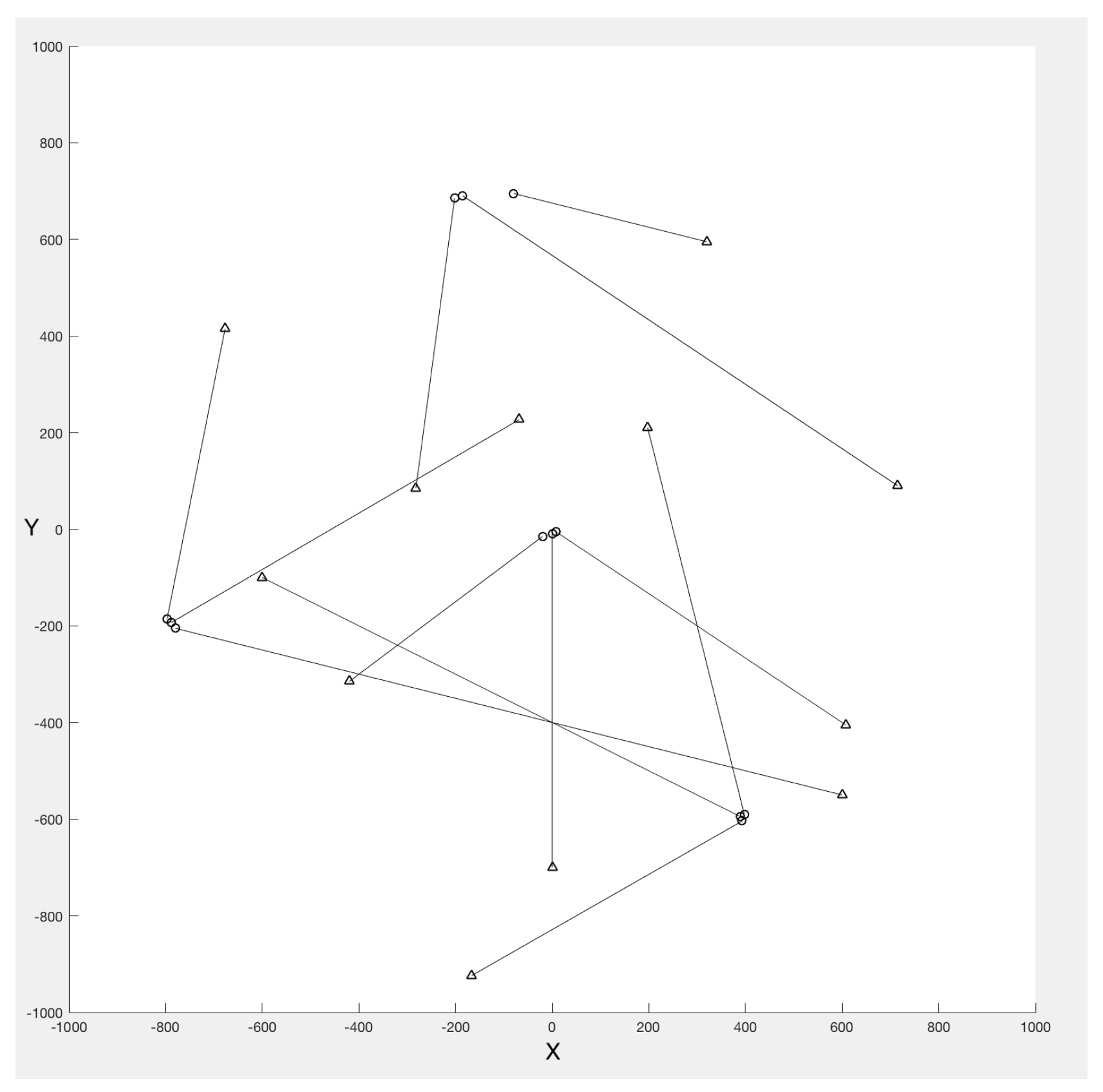
Figure 2.
Different probability of detection (100 Monte Carlo trials). As clear in the figure the proposed methods are outperforming the -GLMB method in the presence of miss detection. With higher rate of miss detection (lower probability of detection) the divergence between different methods increase which shows the power of proposed method in more uncertain conditions like presence of clutter.
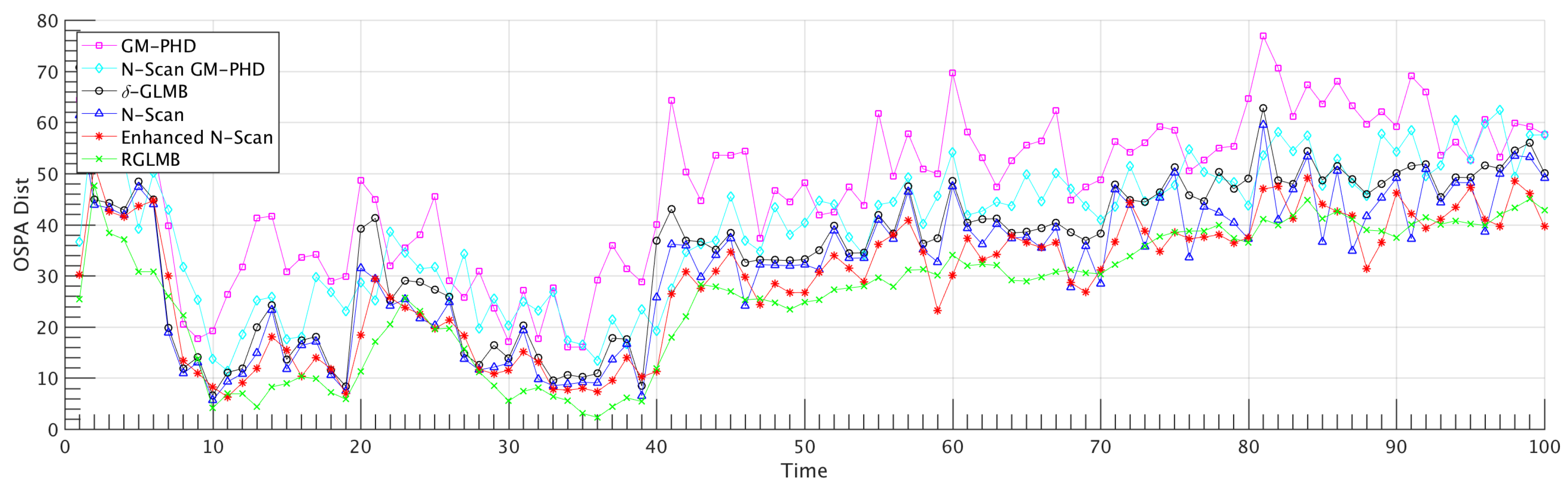
Figure 3.
Different clutter per frame with probability of detection 0.95 (100 Monte Carlo trials). As clear in the figure the proposed methods are outperforming the -GLMB method in the presence of clutter. With higher rate of clutter the divergence between different methods increase which shows the power of proposed method in more uncertain conditions like presence of miss detection.
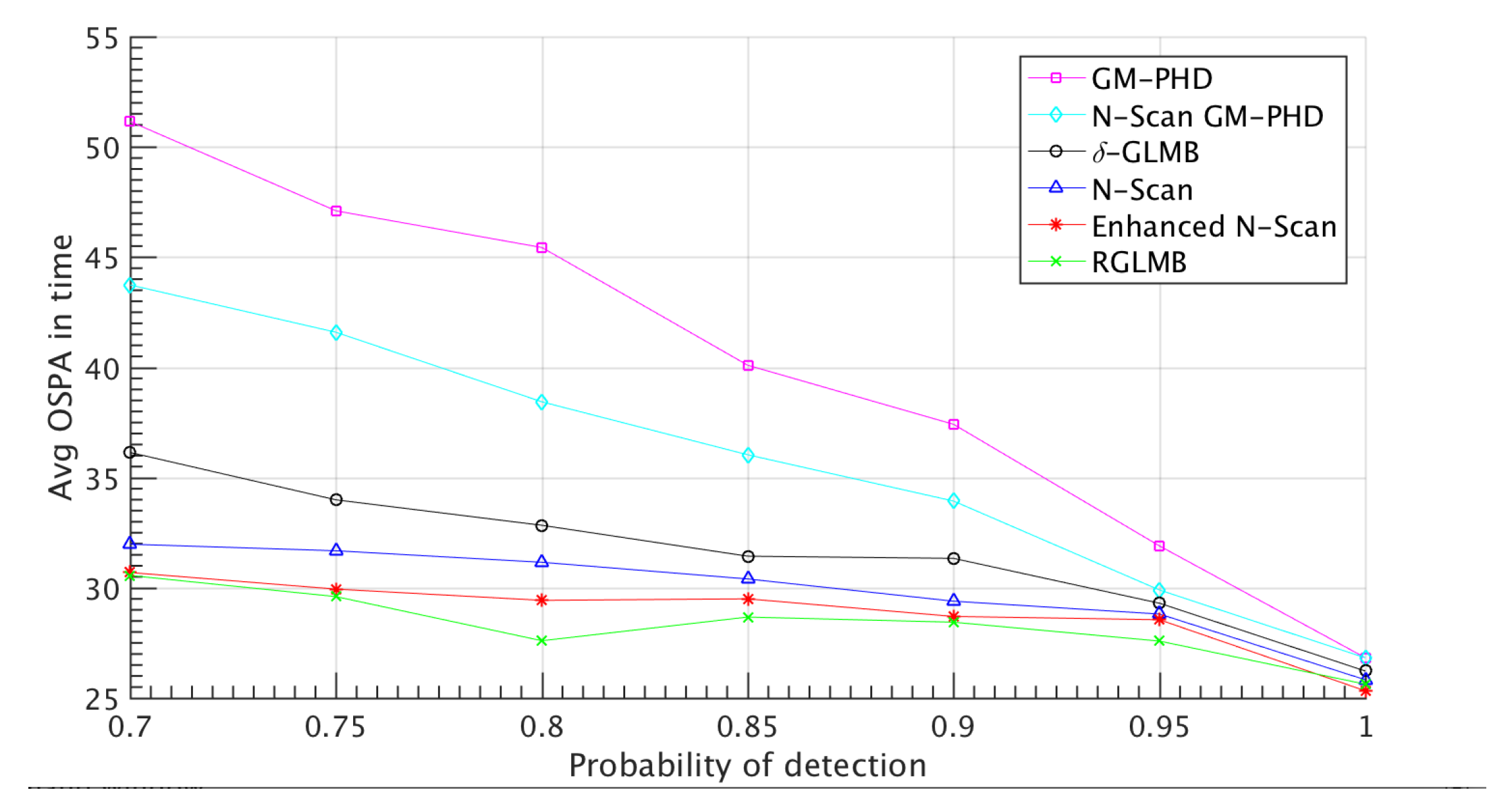
Figure 4.
Different forced consequent miss detection with (100 Monte Carlo trials). This figure shows the examination of proposed method in a condition that miss detection happens consequently which as it is clear in the figure refined GLMB out performs other methods.
Figure 4.
Different forced consequent miss detection with (100 Monte Carlo trials). This figure shows the examination of proposed method in a condition that miss detection happens consequently which as it is clear in the figure refined GLMB out performs other methods.
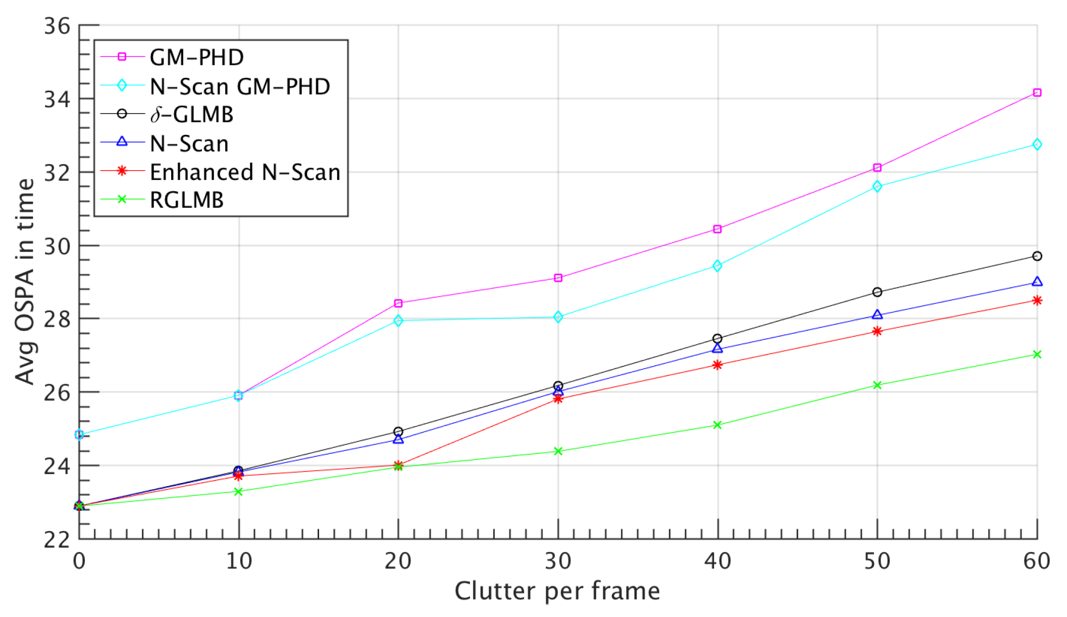
Figure 5.
Multiple trajectories in X-Time and Y-Time plane which are highly occluded and the amount of uncertainty in the measurements are clearly intense.
Figure 5.
Multiple trajectories in X-Time and Y-Time plane which are highly occluded and the amount of uncertainty in the measurements are clearly intense.
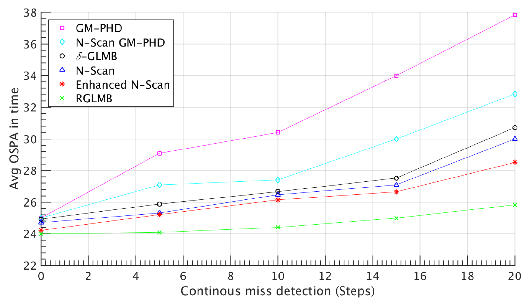
Figure 6.
Results on PETS09-S2L1 (first row) and GRAM-RTM (Urban1) (second row). For simplicity just two targets trajectories are drawn in the pictures. Col one) Trajectory for -GLMB method. Col two) Trajectory for N-scan method. Col three) Trajectory for Enhanced method. Col four) Trajectory for Refined -GLMB.
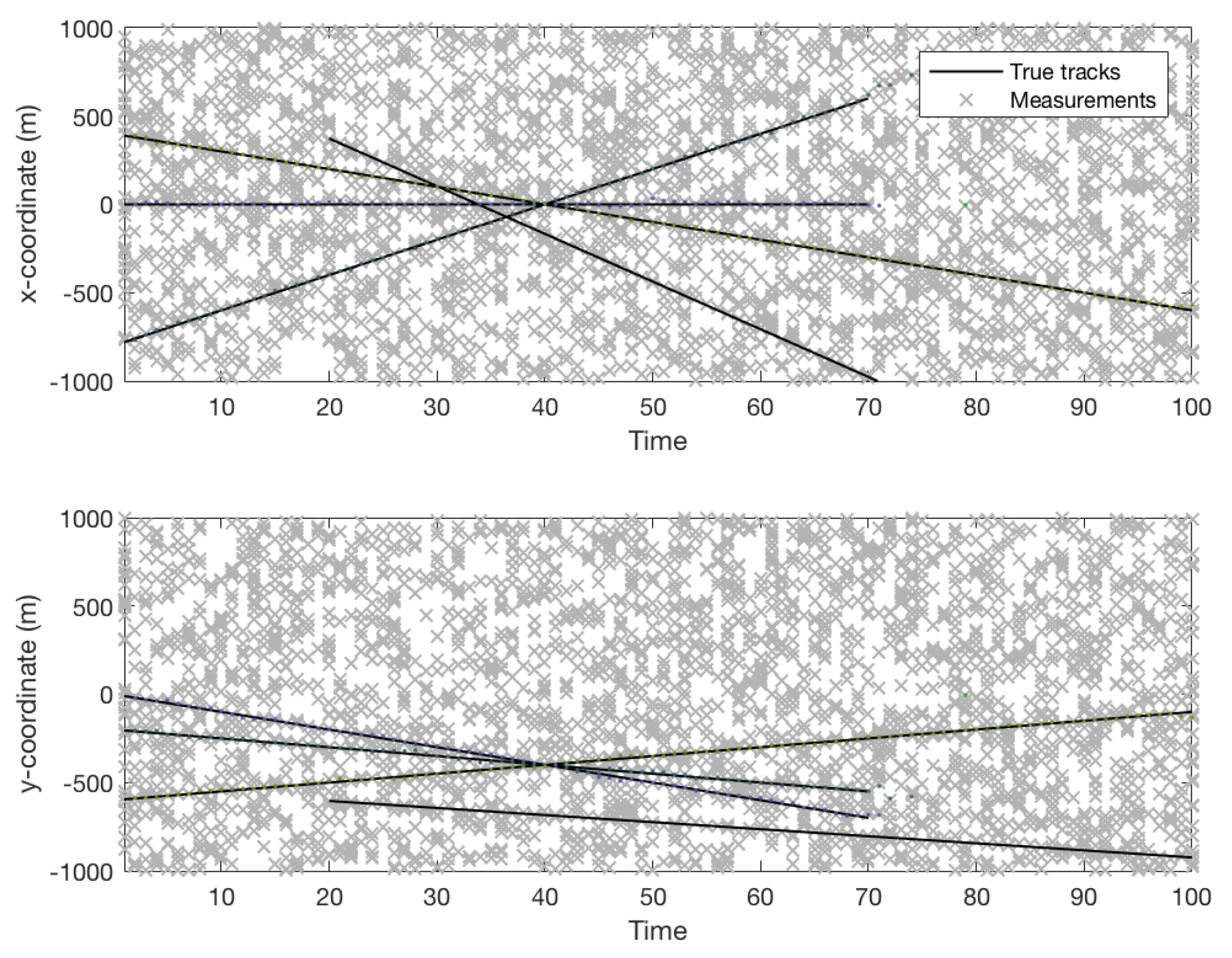
Figure 7.
Results onPETS09-S2L1 (firstrow) and GRAM-RTM (Urban1) (secondrow). For simplicity just two targets trajectories are drawn in the pictures. Col one) Trajectory for δ-GLMB method. Col two) Trajectory for N-scan method. Col three) Trajectory for Enhanced method. Col four) Trajectory for Refined δ-GLMB
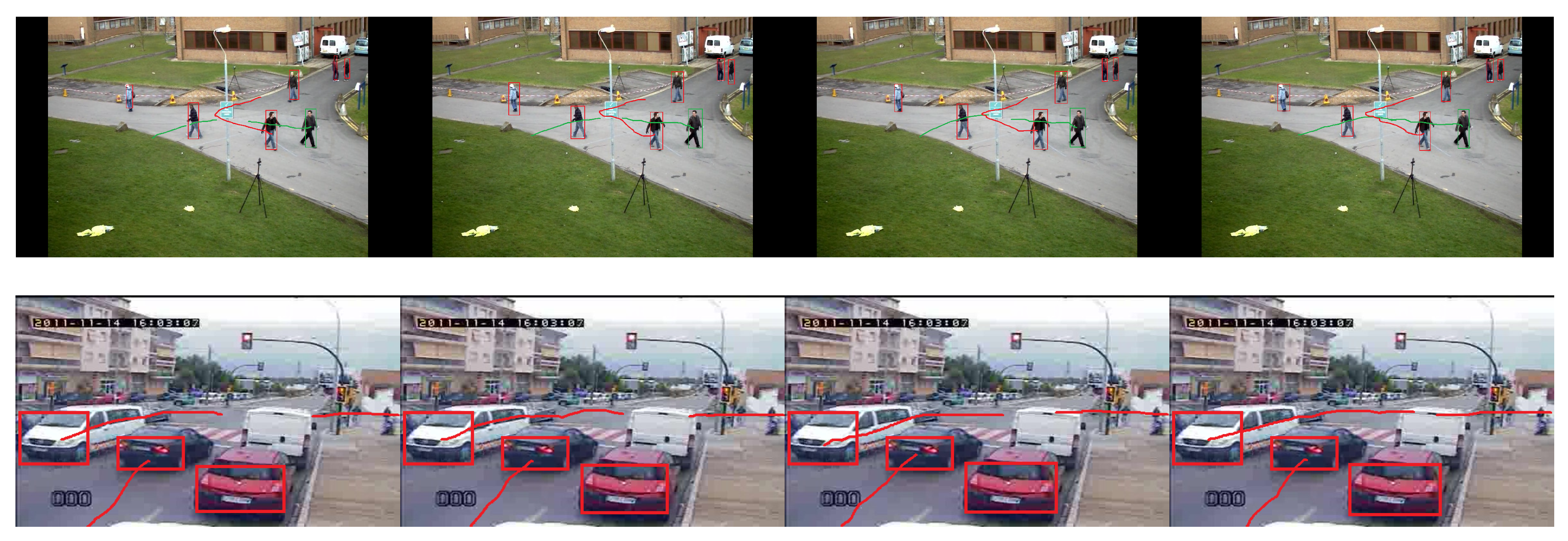
Table 2.
AVG OSPA of different methods in 100 filtering iteration for the scenario defined in fig:6
| Method | OSPA(AVG) |
|---|---|
| GM-PHD | 39.03 |
| N-Scan GM-PHD | 34.51 |
| -GLMB | 32.28 |
| N-scan -GLMB | 28.67 |
| Enhanced N-scan -GLMB | 26.44 |
| Refined N-scan -GLMB | 24.10 |
Disclaimer/Publisher’s Note: The statements, opinions and data contained in all publications are solely those of the individual author(s) and contributor(s) and not of MDPI and/or the editor(s). MDPI and/or the editor(s) disclaim responsibility for any injury to people or property resulting from any ideas, methods, instructions or products referred to in the content. |
© 2025 by the authors. Licensee MDPI, Basel, Switzerland. This article is an open access article distributed under the terms and conditions of the Creative Commons Attribution (CC BY) license (http://creativecommons.org/licenses/by/4.0/).
Copyright: This open access article is published under a Creative Commons CC BY 4.0 license, which permit the free download, distribution, and reuse, provided that the author and preprint are cited in any reuse.


