
Submitted:
21 February 2025
Posted:
21 February 2025
You are already at the latest version
Abstract
This paper present seven uniformly smooth approximating function for absolute value function: five of them approximate absolute value function from above, and the others approximate absolute value function from below. The properties of these uniformly smooth approximating functions are studied, and approximation degree are analyzed in theory and demonstrated by images. Finally, application prospect of uniformly smooth approximating function is pointed out.
Keywords:
absolute value function
; uniformly smooth approximating function
; approximation degree
1. Introduction
The absolute value function is not differentiable at . Absolute value function is of great significance in non-smooth optimization theory and variational inequality. Therefore, it is of great practical significance to study the smooth approximation function of absolute value function. is equivalent to . Literature [7] gave the smoothing processing method of absolute value function and its application in friction contact problems. Some approximation functions of absolute value function are gave in literature [8,9,10,11,12,13], and applied to solve absolute value equation respectively. Literature [14] studied a class of smooth approximation functions of maximum function . Literature [15] studied the uniformly smooth approximation function for absolute value function.
On the basis of the above literatures, this paper systematically gives seven uniformly smooth approximation functions of absolute value functions, analyzes the properties and approximation degrees of these smooth approximation functions theoretically, and finally points out the application prospects of uniformly smooth approximation functions.
Definition 1 (Smooth approximation function [15].) Given a non-smooth function.We call the smooth function the smooth approximation function of . If for any , there exists , such that
If does not depend on , then is said to be a uniformly smooth approximation function of .
Uniformly smooth approximation function can be divided into two classes: from above and from below. Let be the uniformly smooth approximation function of . If satisfies , and, then is said to be uniformly approximated from above. If satisfies , and , then is said to be uniformly approximated from below. The following we use to express .
2. Some Uniformly Smooth Approximating Functions
Following we give seven uniformly smooth approximating functions of the absolute value function . They are continuously differentiable on , and are defined as follows:
2.1. Properties of Function
Proposition 2.1 The function on has the following properties:
(1);
(2) is differentiable on , and
, .
(3) decreases with decreasing parameter , and when, .
Proof (1)
Since , then , and at least one of and is equal to 0, thus ,. So .
Thereby . So .
(2) A simple calculation leads to
Since and are continuous on .Therefore, is differentiable on . And
.
(3)To prove that the decreases with decreasing parameter , it is sufficient to prove that (see Appendix 1). Use, combined with Squeeze Theorem. Then there is.
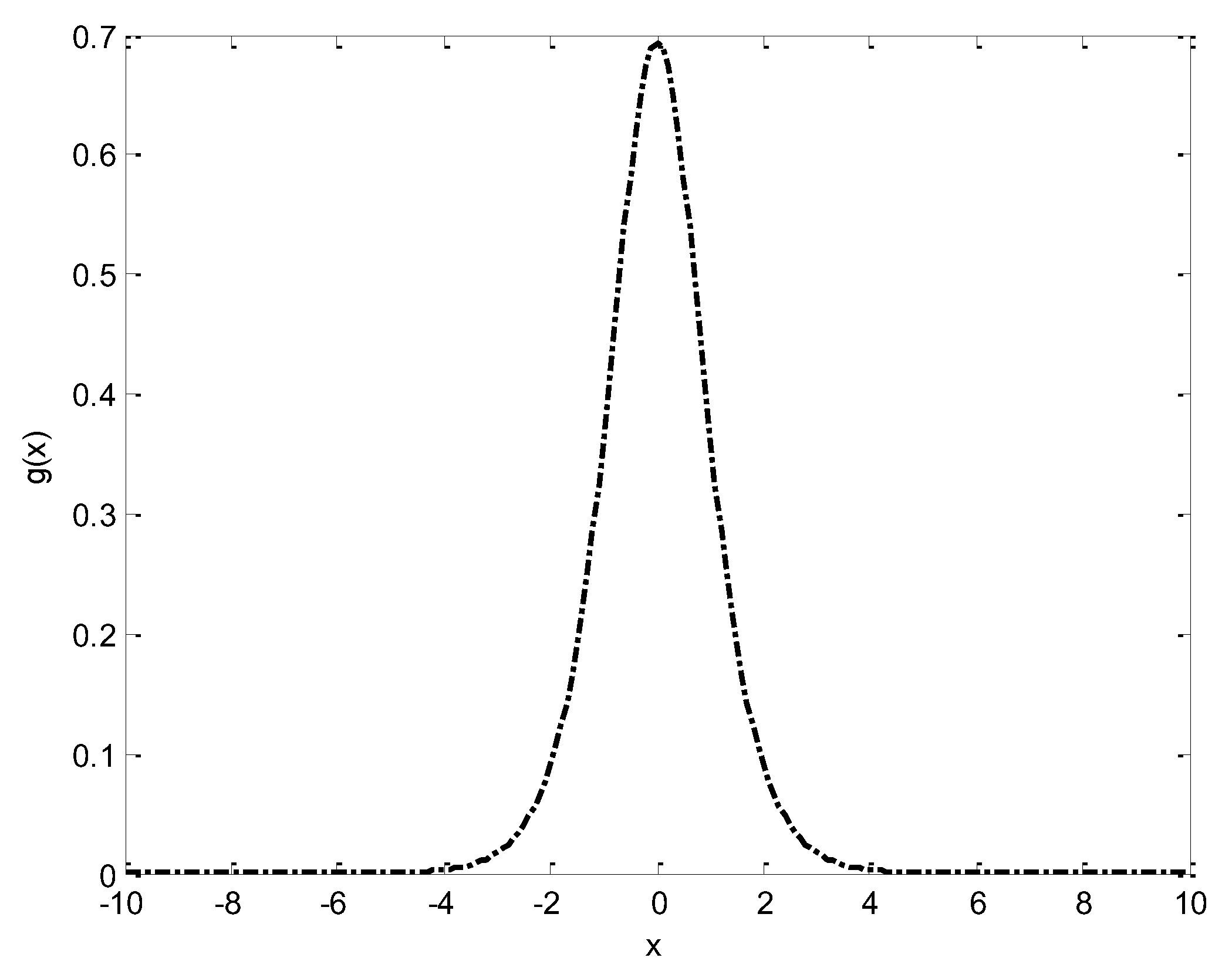
Figure 1 gives the graph of and ,when.It can also be observed from the figure, is uniformly approximates from above.
2.2. Properties of Function
Proposition 2.2 The function in has the following properties:
(1);
(2) is differentiable on ,and
, .
(3) decreases with the decrease parameter ,and when.
Proof (1) Since ,then.
(2) A simple calculation leads to
Apparently, and is continuous, so is differentiable on . And
(3) For any , .Thus the value of decreases with the decrease parameter . Using , combined with Squeeze Theorem. Then there is.
Figure 2 gives the graph of and ,when.It can also be observed from the figure, is uniformly approximates from above.
2.3. Properties of Function
Proposition 2.3 The function in has the following properties:
(1).
(2) is differentiable on ,and
, .
(3) decreases with the decrease parameter ,and when.
Proof (1).
Since ,then , and at least one of and is equal to 0,so.Thus.That is
.
(2)A simple calculation leads to
.
Since and continuous on .So is differentiable on . And
, .
(3) To prove that the value of decreases with decreasing parameter . It is sufficient to prove that (see Appendix 2).
Using, combined with Squeeze Theorem, thus .
Figure 3 gives the graph of and ,when.It can also be observed from the figure, is uniformly approximates from above.
2.4. Properties of Function
Proposition 2.4 The function in has the following properties:
(1);
(2) is differentiable on ,and
,.
(3) decreases with the decrease parameter ,and when.
Proof (1) When,. When ,
.
Thus, for any, we have .
(2) A simple calculation gives
Since ,,so is continuous. Since ,so is continuous. Thus is differentiable on . From the expression for , we get and.
(3) To prove that the value of decreases with decreasing parameter . Only proof is required (see Appendix 3).
Using , combined with Squeeze, thus .
Figure 4 gives the graph of and ,when.It can also be observed from the figure, is uniformly approximates from above.
2.5. Properties of Function
Proposition 2.5 The function in has the following properties:
(1) ;
(2) is differentiable on ,and
,.
(3) decreases with the decrease parameter ,and when.
Proof (1)When,.When ,, while . So when, .
From above, for any,we have .
(2) Simple calculation gives
Since , so is continuous. Since
,
So is continuous. Thus, is differentiable on . From the expression of, we have and .
(3)When,, so This indicates that decreases with the decrease parameter .
Using ,combined with Squeeze Theorem, thus.
Figure 5 gives the graph of and ,when.It can also be observed from the figure, is uniformly approximates from above.
2.6. Properties of Function
Proposition 2.6 The function in has the following properties:
(1);
(2) is differentiable on , and
,且.
(3) increases with decreasing parameter . When,.
Proof (1)When ,. When , . Using the properties of the parabolic function yields , so .
Form above, for any,we have .
(2) A simple calculation gives
Since . thus is continuous. Since
Thus is continuous. So is differentiable on . From the expression of ,we have and .
(3)For any , there are . So increases with decreasing parameter . Using , combined with Squeeze Theorem, thus.
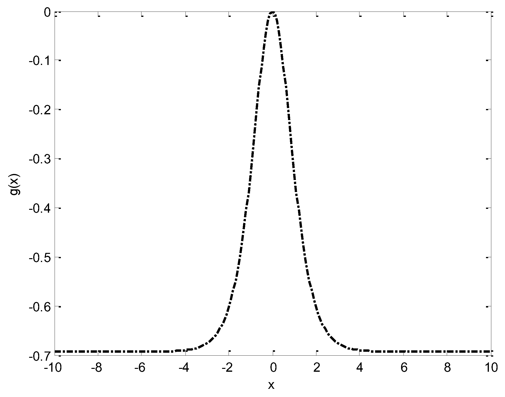
Figure 6 gives the graph of and ,when.It can also be observed from the figure, is uniformly approximates from below.
2.7. Properties of Function
Proposition 2.7 The function in has the following properties:
(1);
(2) is differentiable on ,and
, .
(3) increases with decreasing parameter . When,.
Proof (1),.
Combined .Then there are .
(2) Simple calculation gives
.
So and .
(3) To prove that the value of increases with decreasing parameter . It is sufficient to prove (see Appendix 4).
Using , combined with Squeeze Theorem,thus .
Figure 7 gives the graph of and ,when.It can also be observed from the figure, is uniformly approximates from below.
Some properties of these 7 uniformly smooth approximate functions are given above, and the common properties of these 7 uniformly smooth approximation functions are given in the form of theorems.
Theorem 2.1 , as defined above, satisfies the following properties:
(1) is uniformly smooth approximate function of on . Among which is uniformly smooth approximate functions of from above, while is uniformly smooth approximate functions of from below.
(2) is continuously differentiable on , and all satisfies
,.
(3) For any ,.
3. Approximation Degree of Uniformly Smooth Approximation Function
Following we describes the approximation degree between the and on .From Theorem 2.1 and Figure 5, we can see that approximates most well. To prove this conclusion, firstly we define the distance between two real-valued functions by using infinite norm, that is, for the given two real-valued functions and ,we define the distance between them as
For any given .Since:
and
Since
,
Thus
Therefore, it is concluded from the above approximation we get
.
Thus, approximates most well among .
In fact, for any fixed ,
On the other hand, for any,since
It means
Thus
In addition
.
It means
Thus
.
Therefore, it is concluded from the below approximation that
.
It shows that in all the lower approximation functions , approximates best to . In fact, for any fixed ,
In summary, we have the following conclusions
.
Following, the images of and are given respectively with .
Figure 8.
Graph of and ,when.
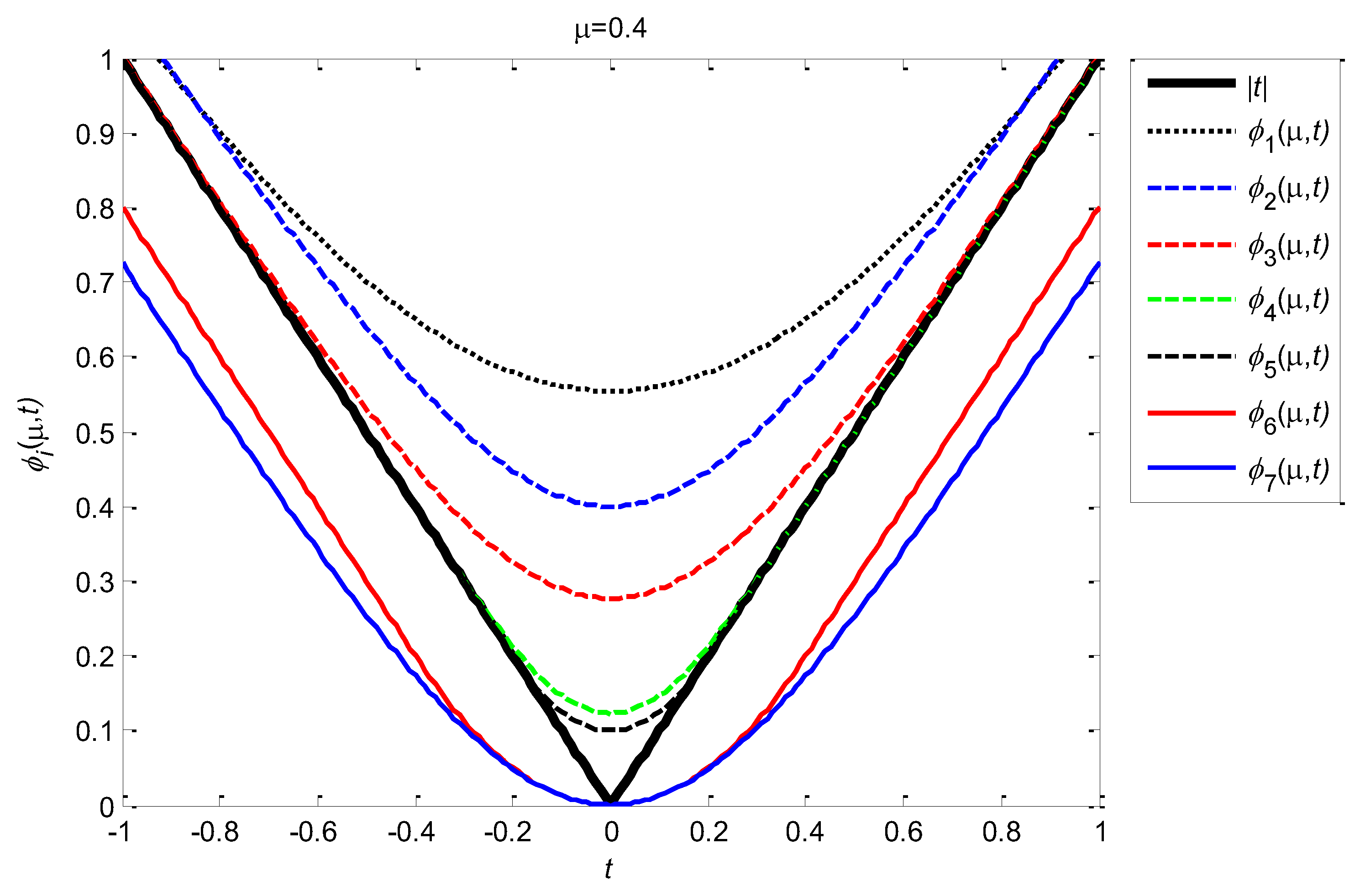
Figure 9.
Graph of and ,when.
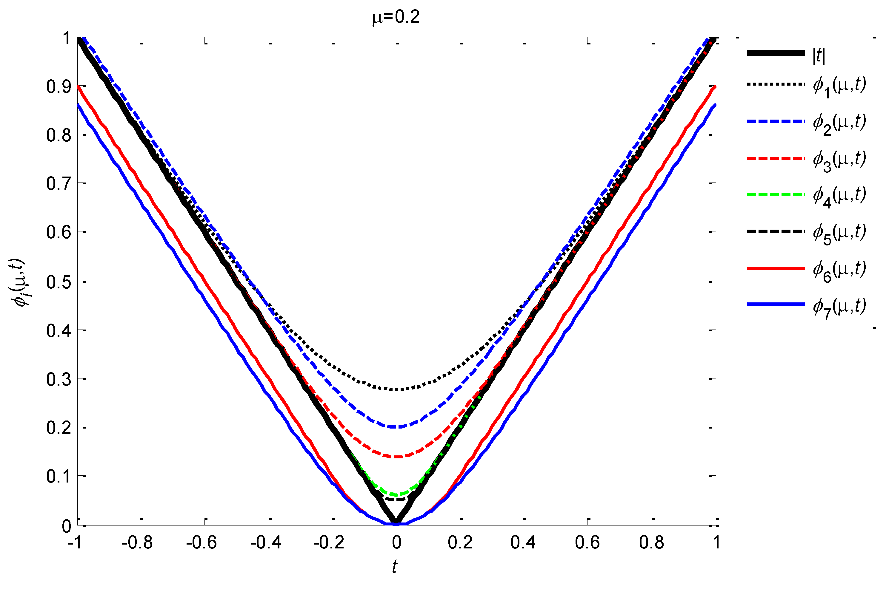
Figure 10.
Graph of and ,when.
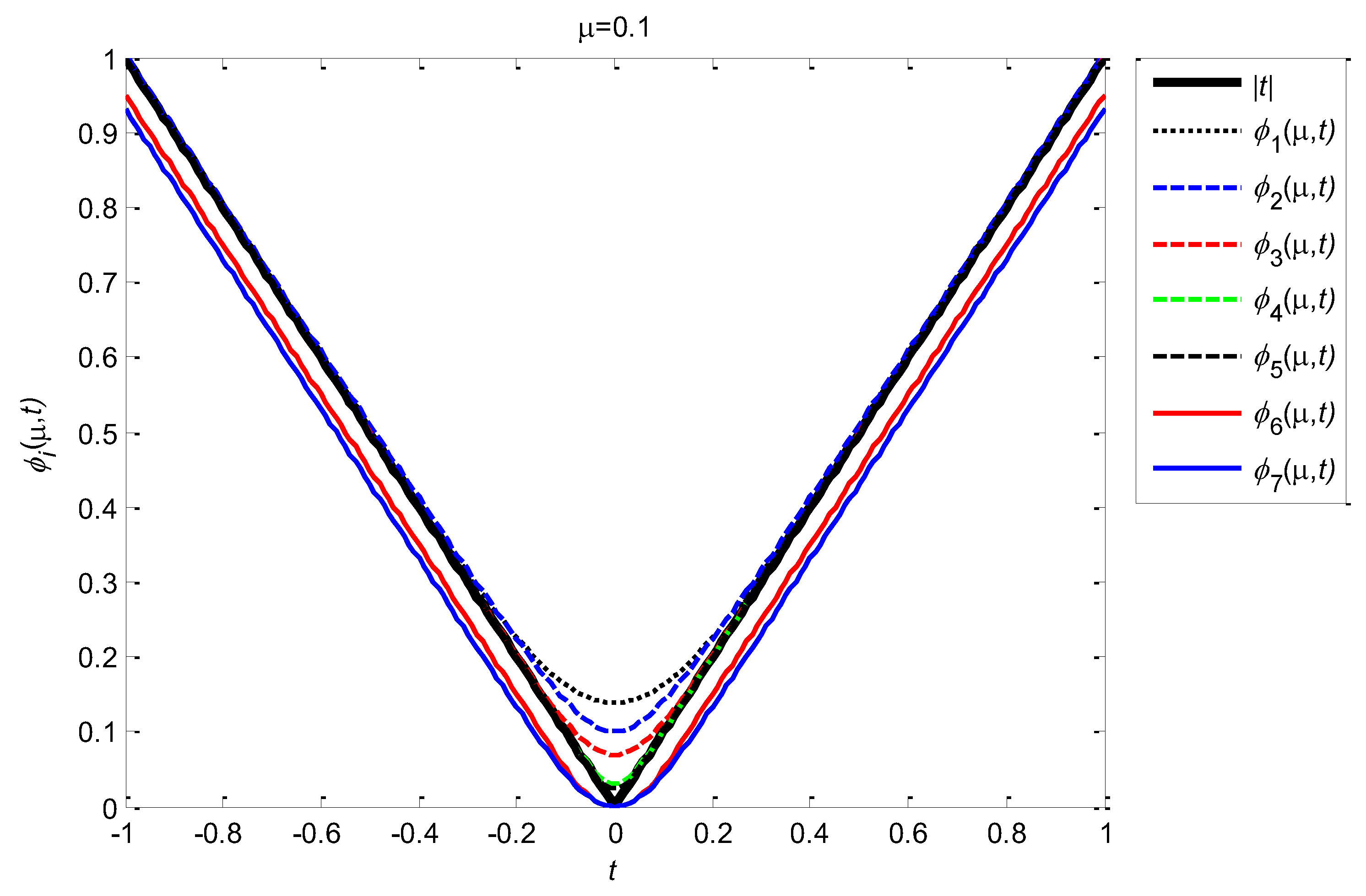
Table 1 gives the distance between and when takes different values.
It can also be derived from the data in Table 1 that the distance between and is the smallest, thus approximates most well.
4. Conclusions
The uniformly smooth approximation function of absolute value function plays important scientific significance in the fields of numerical approximation[16], non-smooth optimization[17], neural network [18,19,20], etc. Limited by space, the application of uniformly smooth approximation functions for absolute value functions will be discussed separately. In addition, among the above uniformly smooth approximation function ,the approximation degree will be better if is replaced by its equivalent infinitesimal quantity .
Funding
This research received no external funding.
Institutional Review Board Statement
Not applicable.
Informed Consent Statement
Not applicable.
Data Availability Statement
The data used to support the findings of this study are available from the corresponding author upon request.
Acknowledgments
This work is supported by Natural Science Foundation of Shaanxi Province(2024JC-YBMS-014), and the Foundation of Shaanxi University of Technology (SLGNL202409).
Conflicts of Interest
The author declares that there is no conflict of interest regarding the publication of this paper.
4. Some Appendixes
Appendix 1
,
Following we prove .
Proof For an any , we need to prove
.
Let , .
Thus we only need to prove .
Since ,.
For any, when ,; when ,, and
.
Thus we have, that is .
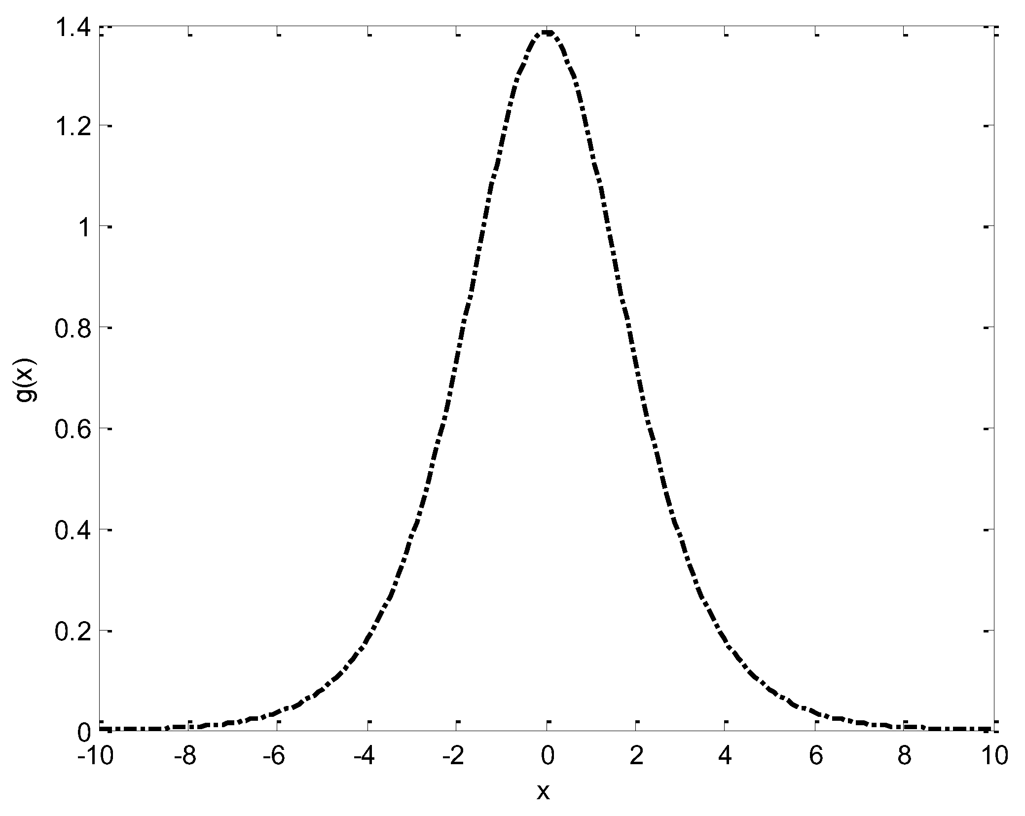
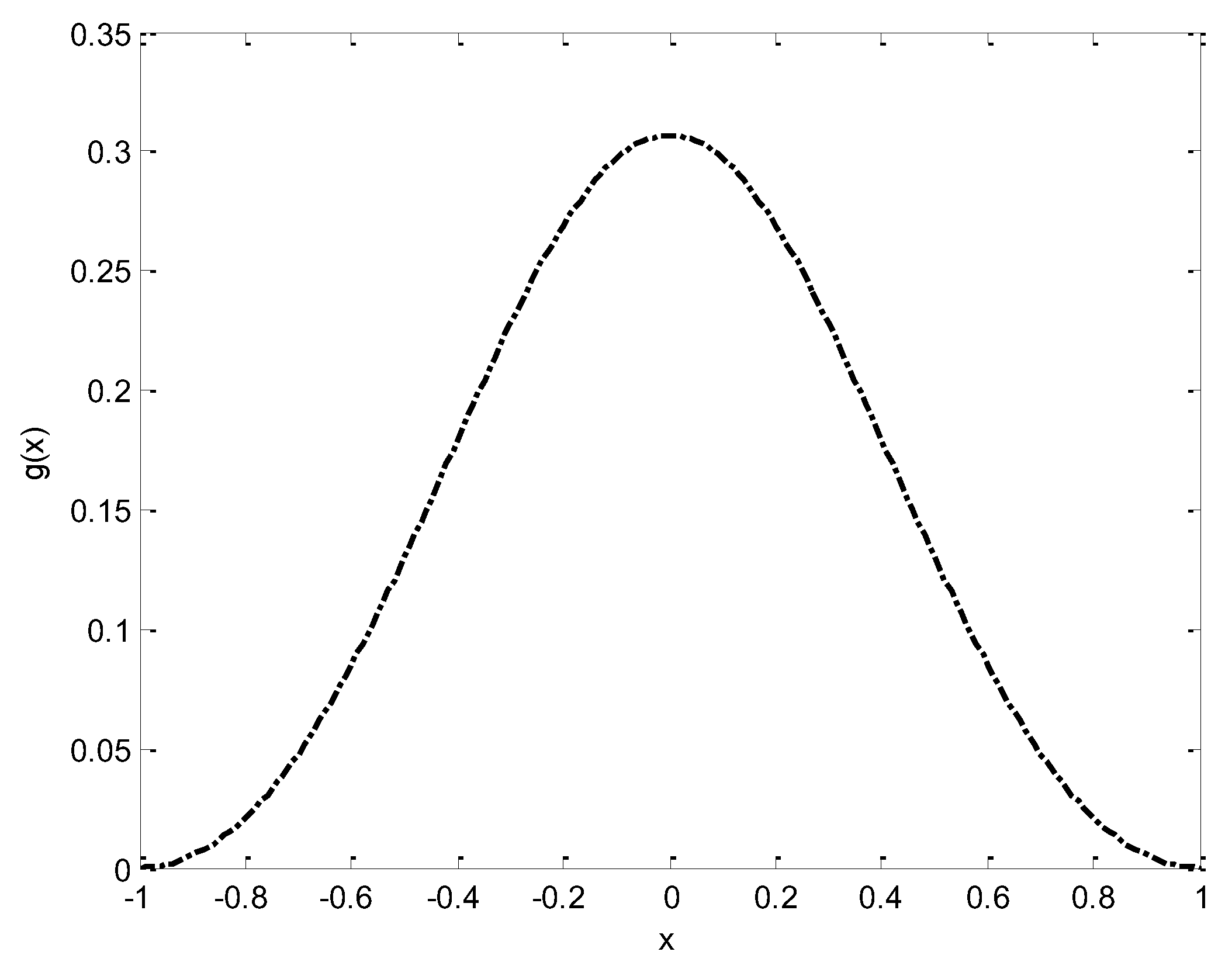
The image of with is shown in the Figure A1.
Figure A1.
The image of with .
Appendix 2
.
Following we prove .
Proof For any, we need to prove
.
Let
,.
Thus we only need to prove .
Since ,.
For any,when ,,when ,, and
.
Thus we have , that is .
The image of with is shown in the Figure A2.
Figure A2.
The image of with .
Appendix 3
Following we prove .
Proof It is only necessary to prove that for any
Let
,.
Thus we only need to prove .
Since ,.
For any,when ,,when ,.
So when ,, when , .
Thus when , , the image of is shown in the Figure A3.
Figure A3.
The image of with .
Appendix 4
Following we prove .
Proof For any, we need to prove
.
Let
, .
Thus we only need to prove .
Since ,.
For any,when ,, thus . When , , so . In addition, .
The image of with is shown in the Figure A4.
Figure A4.
The image of with .
References
- Chen C, Mangasarian O L. A class of smoothing functions for nonlinear and mixed complementarity problems [J]. Computational Optimization and Applications 1996, 5, 97–138. [Google Scholar] [CrossRef]
- Qi L, Sun D. Smoothing Functions and A Smoothing Newton Method for Complementarity and Variational Inequality Problems [J]. Journal of Optimization Theory and Applications 2002, 113, 121–147. [Google Scholar] [CrossRef]
- Qi L, Chen X. A Globally Convergent Successive Approximation Method for Severely Nonsmooth Equations [J]. SIAM Journal on Control & Optimization 2006, 33, 402–418. [Google Scholar]
- Huang Z H, Zhang Y, Wu W. A smoothing-type algorithm for solving system of inequalities [J]. Journal of Computational & Applied Mathematics 2008, 220, 355–363. [Google Scholar]
- Zhang Y, Huang Z H. A nonmonotone smoothing-type algorithm for solving a system of equalities and inequalities [J]. Journal of Computational & Applied Mathematics 2010, 233, 2312–2321. [Google Scholar]
- Wang F, Yu Z, Gao C. A Smoothing Neural Network Algorithm for Absolute Value Equations [J]. Engineering 2015, 7, 567–576. [Google Scholar] [CrossRef]
- Zhang Hongwu, He Suyan, Li Xingsi. Non-Interior Smoothing Algorithm for Frictional Contact Problems[J]. Applied Mathematics and Mechanics 2004, 25, 42–52. [Google Scholar]
- Louis Caccetta, Biao Qu,Guanglu Zhou. A globally and quadratically convergent method for absolute value equations [J]. Computational Optimization and Applications. 2011, 48, 45–58. [Google Scholar] [CrossRef]
- Yong Longquan, Tuo Shouheng. Quasi-Newton method for absolute value equations based aggregate function[J]. Journal of Systems Science and Mathematical Sciences 2012, 32, 1427–1436. [Google Scholar]
- Esmaeili H, Mahmoodabadi E, Ahmadi M. A uniform approximation method to solve absolute value equation [J]. Bulletin of the Iranian Mathematical Society 2015, 41, 1259–1269. [Google Scholar]
- Yong Long-quan. A smooth Newton method to absolute value equation based on adjustable entropy function[J]. Journal of Lanzhou University: Natural Sciences 2016, 52, 540–544. [Google Scholar]
- Longquan Yong. A Smoothing Newton Method for Absolute Value Equation [J]. International Journal of Control and Automation 2016, 9, 119–132. [Google Scholar] [CrossRef]
- Saheya B, Yu C H, Chen J S. Numerical comparisons based on four smoothing functions for absolute value equation[J]. Journal of Applied Mathematics & Computing 2016, 1–19.
- Zhang Lili, Li Jianyu, Li Xingsi. Some Properties of a Smoothing Approximation for Maximum Function[J]. Mathematics in Practice and Theory 2008, 38, 229–234. [Google Scholar]
- Yong Longquan. Uniform Smooth Approximation Functions for absolute value function[J]. Mathematics in Practice and Theory 2015, 45, 250–255. [Google Scholar]
- Wang Renhong. Numerical Approximation [M]. Higher Education Press, 1999.
- Sahoya. Research on Cone model method of nonlinear equations [D]. Hohhot: Inner Mongolia University, 2017: 69-78.
- Chen J S, Ko C H, Pan S. A neural network based on the generalized Fischer–Burmeister function for nonlinear complementarity problems [J]. Information Sciences 2010, 180, 697–711. [Google Scholar] [CrossRef]
- Sun J, Chen J S, Ko C H. Neural networks for solving second-order cone constrained variational inequality problem [J]. Computational Optimization and Applications 2012, 51, 623–648. [Google Scholar] [CrossRef]
- Miao X, Chen J S, Ko C H. A neural network based on the generalized FB function for nonlinear convex programs with second-order cone constraints [J]. Neurocomputing 2016, 203, 62–72. [Google Scholar] [CrossRef]
Figure 1.
Graph of and ,when.
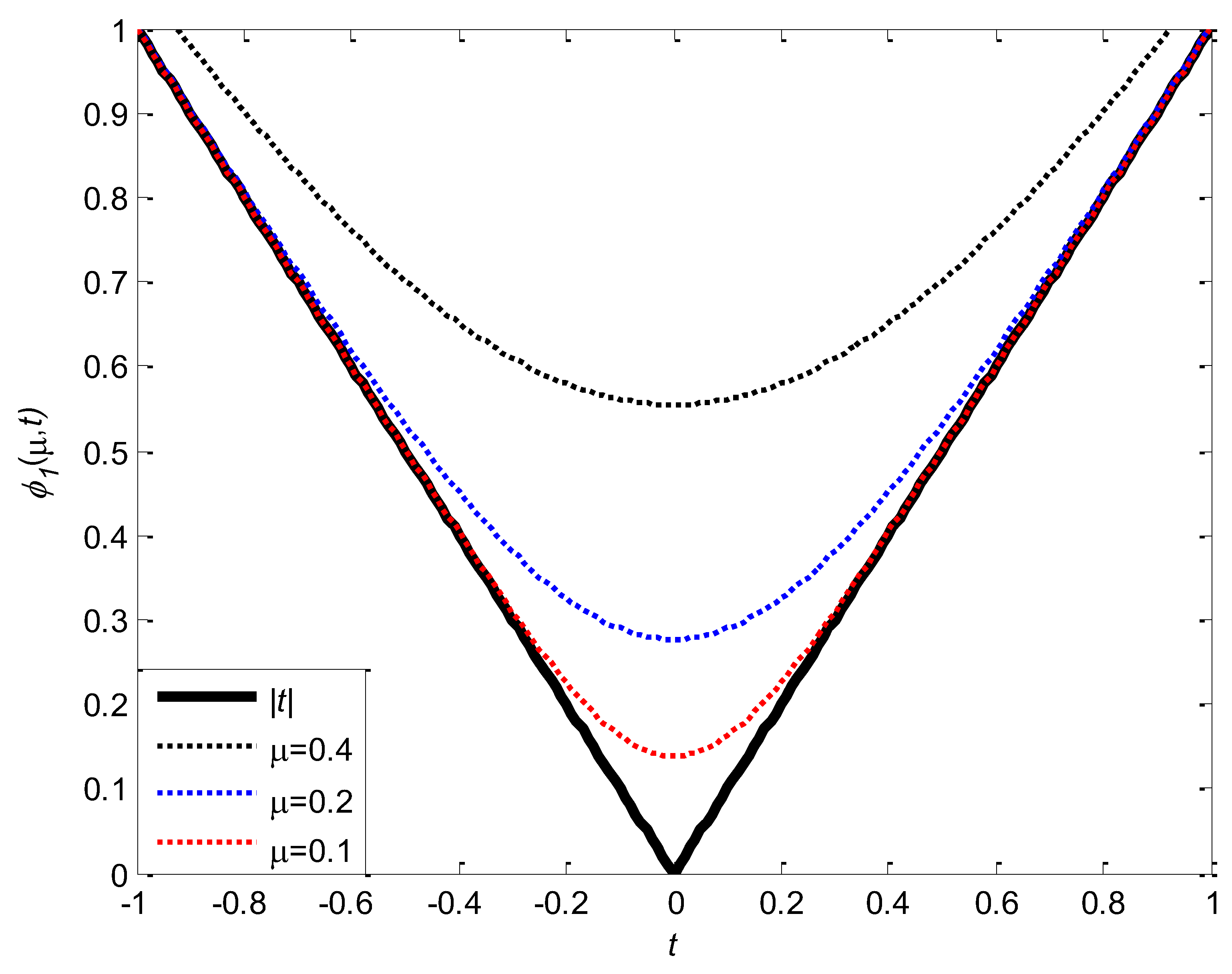
Figure 2.
Graph of and ,when.
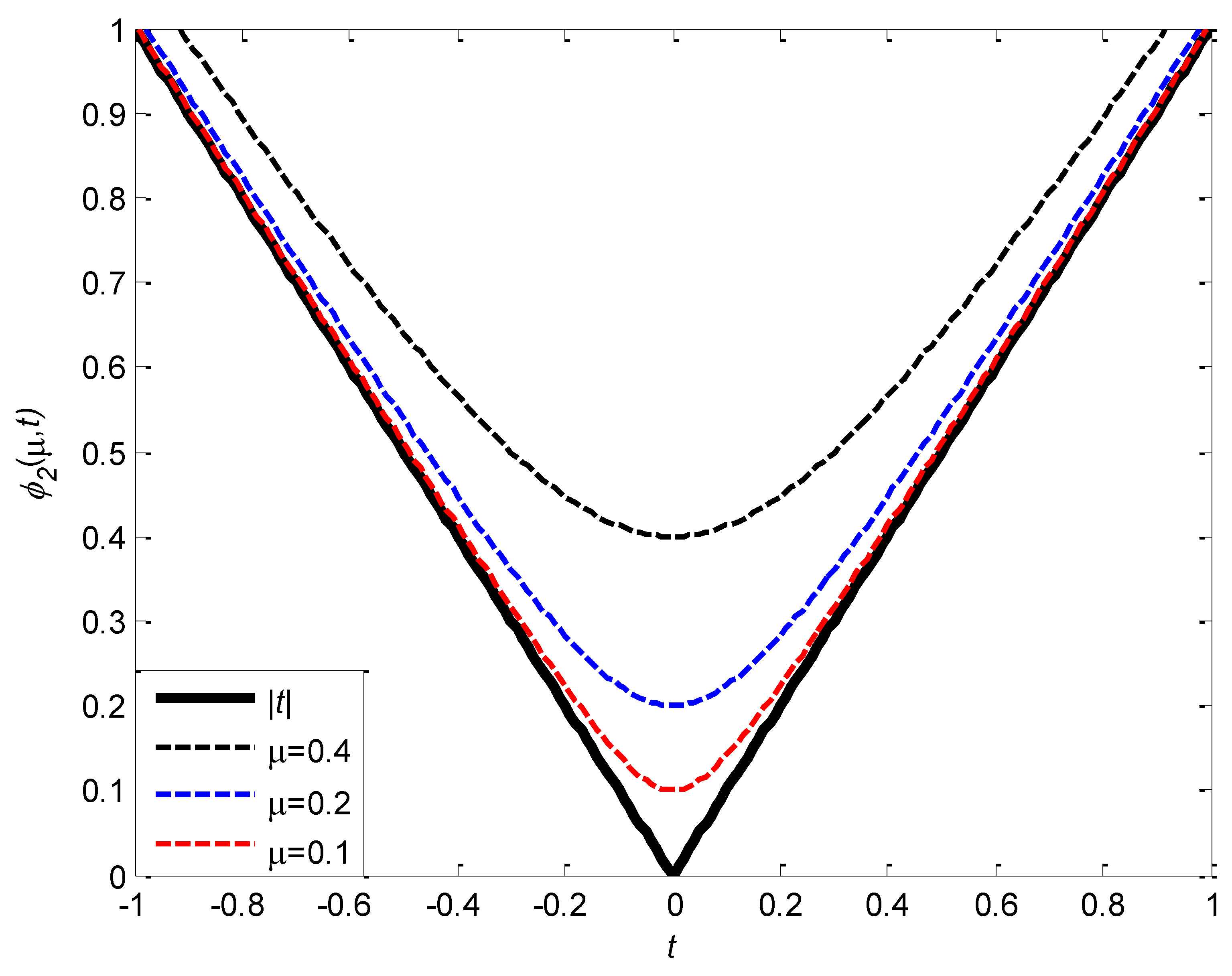
Figure 3.
Graph of and ,when.

Figure 4.
Graph of and ,when.
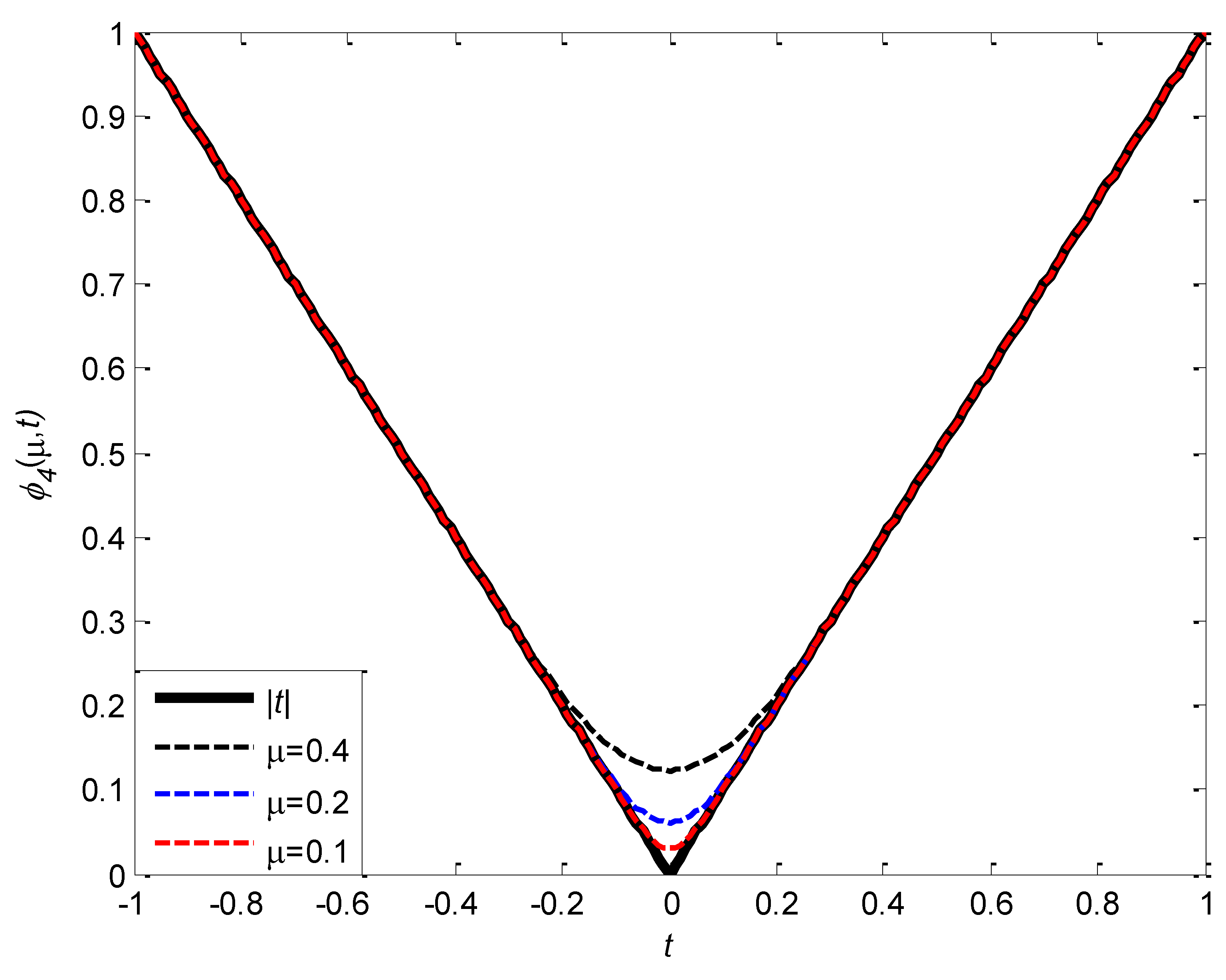
Figure 5.
Graph of and ,when.

Figure 6.
Graph of and ,when.
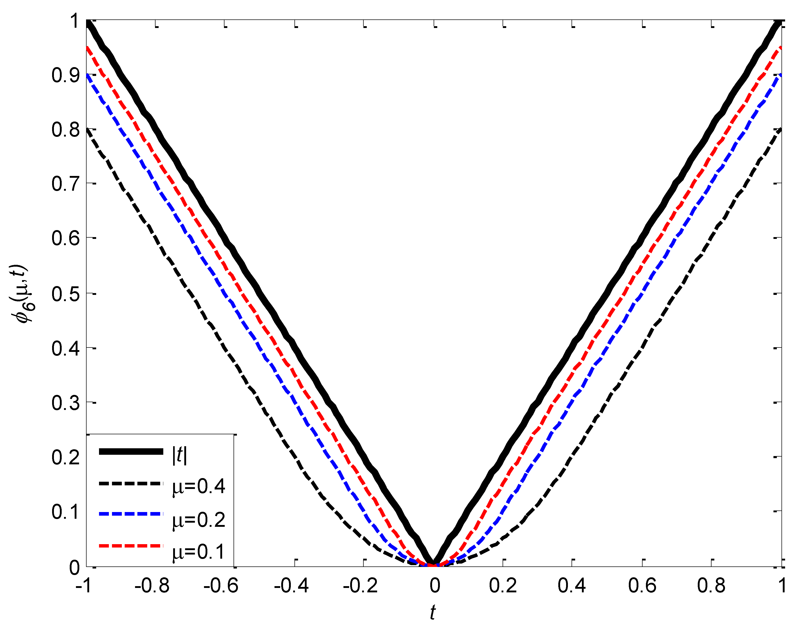
Figure 7.
Graph of and ,when.
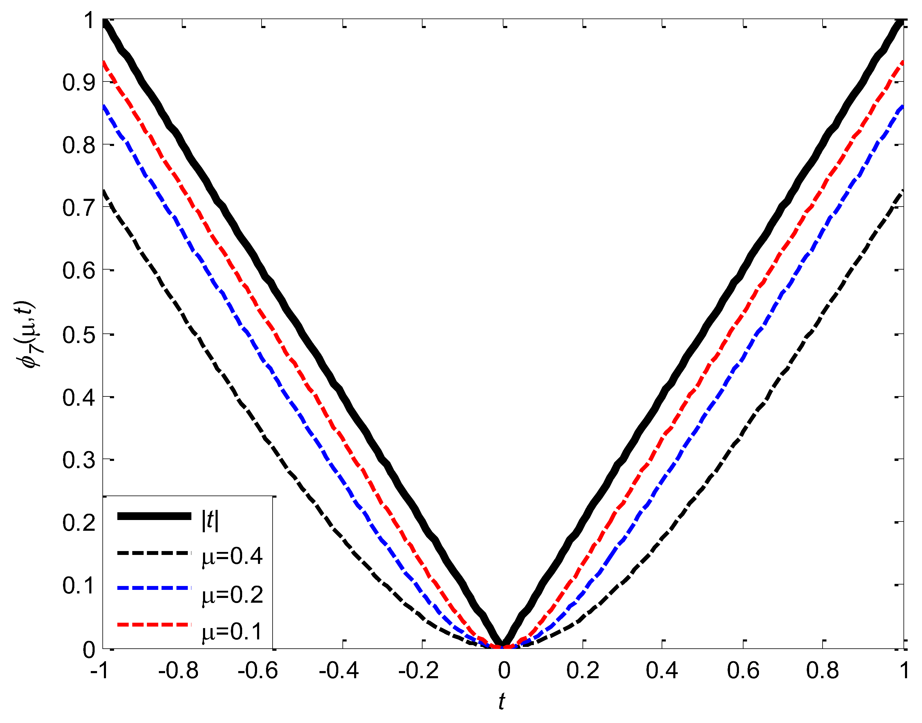

Table 1.
The distance between and .
| 1.3862 | 0.5545 | 0.2772 | 0.1386 | |
| 1.0000 | 0.4000 | 0.2000 | 0.1000 | |
| 0.6931 | 0.2772 | 0.1386 | 0.0693 | |
| 0.3069 | 0.1228 | 0.0614 | 0.0307 | |
| 0.2500 | 0.1000 | 0.0500 | 0.0250 | |
| 0.5000 | 0.2000 | 0.1000 | 0.0500 | |
| 0.6931 | 0.2772 | 0.1386 | 0.0693 |
Disclaimer/Publisher’s Note: The statements, opinions and data contained in all publications are solely those of the individual author(s) and contributor(s) and not of MDPI and/or the editor(s). MDPI and/or the editor(s) disclaim responsibility for any injury to people or property resulting from any ideas, methods, instructions or products referred to in the content. |
© 2025 by the authors. Licensee MDPI, Basel, Switzerland. This article is an open access article distributed under the terms and conditions of the Creative Commons Attribution (CC BY) license (http://creativecommons.org/licenses/by/4.0/).
Copyright: This open access article is published under a Creative Commons CC BY 4.0 license, which permit the free download, distribution, and reuse, provided that the author and preprint are cited in any reuse.


