Submitted:
21 February 2025
Posted:
21 February 2025
You are already at the latest version
Abstract
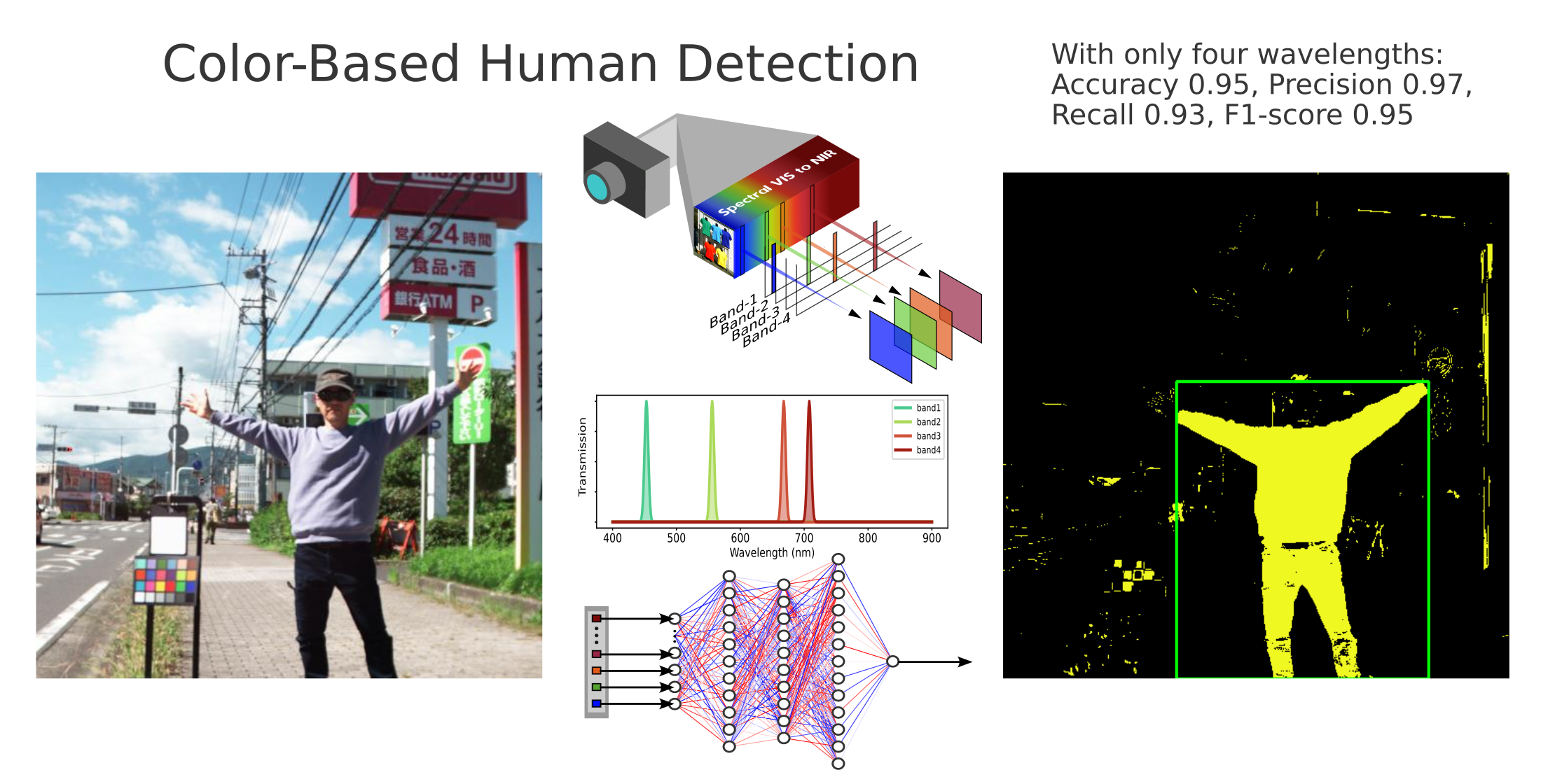
In this study, we propose a color-based multispectral approach using four selected wavelengths (453, 556, 668, and 708 nm) from the visible to near-infrared range to separate clothing from the background. Our goal is to develop a human detection camera that supports real-time processing, particularly under daytime conditions and for common fabrics. While conventional deep learning methods can detect humans accurately, they often require large computational resources and struggle with partially occluded objects. In contrast, we treat clothing detection as a proxy for human detection and construct a lightweight machine learning model (multi-layer perceptron) based on these four wavelengths. Without relying on full spectral data, this method achieves an accuracy of 0.95, precision of 0.97, recall of 0.93, and an F1-score of 0.95. Because our color-driven detection relies on pixel-wise spectral reflectance rather than spatial patterns, it remains computationally efficient. A simple four-band camera configuration could thus facilitate real-time human detection. Potential applications include pedestrian detection in autonomous driving, security surveillance, and disaster victim searches. However, our current results are limited to daytime environments and fibers such as cotton, polyester, and wool.
Keywords:
color imaging
; multispectral imaging
; human detection
; machine learning
; real-time processing
; spectral reflectance
1. Background And Objectives
1.1. Background and Significance
Human detection technologies are important for such applications as autonomous driving, security surveillance, and disaster rescue. At disaster sites, it is crucial to locate victims as quickly as possible. In autonomous driving, pedestrians must be detected accurately. Leveraging spectral characteristics may make it possible to achieve high accuracy with reduced computational load.
In this research, we developed a new human detection approach that uses the spectral (color) properties of clothing. Assuming outdoor daytime conditions and common fibers such as cotton, polyester, and wool, we hypothesize that fibers and dyes exhibit high reflectance in the near-infrared region, which can be exploited to detect people’s clothing with high accuracy. This limitation of fiber types is based on data indicating that cotton, polyester, and wool account for 79.9% of major global fibers [1].
To verify this hypothesis, the aim of this study was to show that, by effectively and simply selecting wavelengths from the visible to near-infrared range, clothing and background can be distinguished. This work serves as an initial study toward realizing a “human detection camera” that can operate in real time.
1.2. Related Previous Studies
Human detection using deep learning
Human detection with visible-light cameras and thermal cameras
The KAIST dataset [7] and the CVC-14 dataset [8] are large-scale pedestrian detection datasets combining visible-light images and thermal images, allowing evaluation of human detection methods under various environments, including daytime and nighttime. Prior work [9] achieved high accuracy and generality by employing a deep learning approach that fuses features from visible and thermal images and takes illumination conditions into account.
However, while thermal imaging has the advantage of using the subject’s temperature distribution, there are also reports of issues such as reduced resolution for pedestrians, misalignment with visible cameras, and the high cost of thermal cameras.
Segmentation using spectral information
In autonomous driving, segmentation based on spectral information has been attempted. For example, datasets such as HyKo [10] and HSI-Drive [11,12] are available. However, they mainly target multi-class segmentation of driving features such as roads and vehicles, and are not necessarily specialized for optimizing wavelength sets to detect clothing [13].
Human detection with SWIR spectral information
Short-wave infrared (SWIR) wavelengths, approximately 900–1,700 nm, can exploit skin reflectance characteristics to reduce the computational load [14]. Nevertheless, SWIR sensors remain expensive (on the order of tens of thousands of dollars), creating hurdles for adoption in consumer-facing applications.
1.3. Concept and Purpose of this Research
Focusing on the property that “clothing tends to show relatively high reflectance in the near-infrared range” [15], we constructed a model that classifies clothing from only four multispectral wavelengths spanning the visible to near-infrared region. Because clothing generally occupies a larger area than skin and differs spectrally from background objects, we hypothesize that human detection can be achieved without incurring the large computational burden of deep learning.
In this study, we focused on daytime outdoor conditions with common fibers, and selected an optimal set of four wavelengths using data acquired through hyperspectral imaging. We also determined that it may be possible to achieve sufficient clothing detection performance with a simple camera configuration of about four bands using a silicon CMOS image sensor in the future.
The academic contributions of this research can be summarized as follows:
-
High-accuracy human detection using four wavelengthsBy selecting only four (narrow) wavelengths in an optimal combination, clothing can be accurately identified without using the entire visible to near-infrared range.
-
Combining dimensionality reduction with random exploration
-
Real-time suitability and simple configurationBecause this method relies on spectral information on a per-pixel basis rather than on spatial patterns, it can offer fast inference and low memory usage. Compared with conventional deep learning methods, there is potential for drastically reduced computational resources.
-
Differences from existing methods and academic significanceExisting approaches based on deep learning for object detection, or methods leveraging SWIR/thermal cameras effective for nighttime detection, have each demonstrated high performance. In contrast, our study could develop a new framework that achieves high accuracy for daytime outdoor clothing detection with minimal sensor and computational costs by using only four wavelengths in the visible–near-infrared range. This addresses low-cost and low-load scenarios not well covered by existing methods, thereby expanding the range of options for future human detection technologies.
1.4. Structure of This Paper
- Section 2 describes the spectral characteristics of clothing.
- Section 3 explains the approach for distinguishing clothing from the background using machine learning, including model selection, the multi-layer perceptron (MLP) workflow, and training conditions.
- Section 4 presents classification experiments using the MLP model and discusses three stages: “full hyperspectral model,” “dimensionality reduction,” and “reduction in the number of bands.”
2. Spectral Characteristics Of Clothing And Outdoor Background
2.1. Hyperspectral Camera Imaging and Terminology
To analyze the spectral reflectance of clothing against a background (inorganic materials and plants), we collected image data using a hyperspectral camera (Specim IQ by Delft Hi-TeC). This camera is equipped with a CMOS sensor covering 400–1,000 nm, featuring 204 bands, a spectral resolution of 7 nm, a spatial resolution of 512 × 512 pixels, and an 8-bit intensity resolution.
We conducted daytime photography under stable illumination, requiring about 10–30 s per capture. Because the camera has limited sensitivity, we restricted this study to still-image data recorded outdoors in daylight; application to nighttime or indoor environments is left for future work.
A white reference board (provided with the camera) was used for calibration, and the Savitzky–Golay method [18] was applied to reduce noise in the acquired spectral data. As data at wavelengths above 900 nm contained a lot of noise, we used only the 400–900 nm range (167 bands) in this study.
In this paper, “spectral reflectance” refers to how much light an object reflects at each wavelength. In our experiments, the method using 167 bands between 400 and 900 nm is referred to as “hyperspectral,” whereas the approach that later selects around 4–12 discrete wavelengths is called “multispectral.” Furthermore, an “optimal wavelength set” (OWS) denotes a combination of wavelengths that maximizes clothing-detection performance. In this study, we explored sets of about four or five bands that showed high performance, and we used them to distinguish clothing from the background.
2.2. Imaging Targets
We took hyperspectral images of 85 types of clothing and 35 cityscape scenes (Figure 1). (Figure 1(b) and (c) show examples of pseudo-color images generated by combining the bands for 650 nm, 530 nm, and 470 nm as RGB. (Henceforth, pseudo-color images are shown by combining these three bands.)
2.2.1. Hyperspectral Images of Clothing
We prepared various garments and fabrics made of cotton, polyester, and wool. These items were dyed with a range of colored dyes. The images of clothing in Figure 1(b) are representative pseudo-color shots of the captured data.
2.2.2. Hyperspectral Images of the Background
As the background, we captured city and suburban landscapes, including roads, grass, wood, concrete, buildings, and vehicles in scenes with both sunny and cloudy daylight conditions. Figure 1(c) shows some examples of these background images in pseudo-color. The objects in the background appear to the human eye as green, gray, brown, and similar colors.
2.3. Observing the Spectra of Clothing and Outdoor Scenes
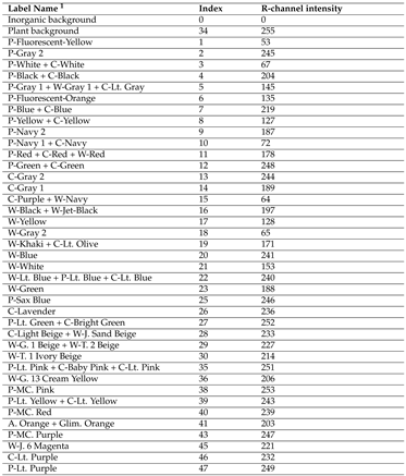
After imaging, we manually labeled target regions to produce label images. Clothing with similar spectral properties was consolidated into 39 labels, while the background was split into two categories—inorganic and plant. Table 1 lists all 41 labels (label name, index number, and R-channel brightness in the labeled image).
Figure 2 shows an example of a labeled image alongside its corresponding pseudo-color image. In the labeled image, the R-channel brightness indicates the label class. For instance, plants are labeled with R = 255, and inorganic background is R = 0. Clothing has 39 distinct R brightness values depending on the fiber and color.
Figure 3 presents the hyperspectral reflectance curves for (a) 39 clothing labels, (b) an inorganic background, and (c) plants.
- In (a) for clothing, dyes absorb light at various visible wavelengths, creating the garment’s color. Meanwhile, nearly all clothing exhibits high reflectance in the near-infrared region, invisible to the human eye.
- In (b), inorganic objects do not show major changes across the visible to near-infrared range; there is almost no tendency for reflectance to rise in the near-infrared region.
- In (c), plants absorb blue light ( nm) and red light ( nm) while reflecting green ( nm), and they have high reflectance in the near-infrared. This is a well-known property of plant hyperspectral reflectance [19].
Thus, clothing and plants both exhibit high reflectance in the near-infrared, suggesting that distinguishing clothing from vegetation based on spectral information alone could be challenging.
3. Classification Of Clothing And Background Using Machine Learning
3.1. Choice of Machine Learning Model
We employed machine learning to perform classification. To handle the variety of clothing, we adopted a multi-label classification model. Using scikit-learn [20], we compared five machine learning models—RBF-SVM, RandomForest, GradientBoosting, AdaBoost, and MLPClassifier [21,22,23,24,25]. As shown in Table 2, RBF-SVM and MLPClassifier gave the highest scores. Taking computational time into account, we ultimately selected the MLP.
In our preliminary experiments to determine the MLP structure using PyTorch Lightning, we varied the number of units in the hidden layers (testing sizes of 6, 10, 16, 32, and 64) while temporarily fixing the input layer to 20 units. We found that using two hidden layers with 16 units each resulted in performance that nearly saturated, while keeping computational cost and memory usage minimal (Table 3). Based on these results, we adopted an architecture comprising two hidden layers of 16 units each and an output layer of 49 units, thereby fixing the hidden and output layer configuration. However, in further experiments we plan to vary only the number of input layer units—while maintaining this optimized configuration—to investigate its impact. (Initially, the PyTorch implementation defined 49 output units; however, after consolidating the clothing labels into 39 categories, there are actually 39 clothing labels plus 2 background labels (i.e., 41 total). Since the unused output units had little effect on the training results, we continued using the 49-unit output design in our experiments.)
3.2. MLP Processing Flow and Training Conditions
Figure 4 illustrates the process of creating the dataset for the MLP. The main steps are as follows:
- Determine the number of wavelengths to use and choose which wavelengths to include, forming an OWS.
- Extract the band images according to this wavelength set.
- Randomly sample pixels from the labeled regions, taking 50 pixels per label for training.
- Pair each pixel’s intensity vector with the corresponding label.
Figure 5 shows an example of sampled pixels (marked in dark green). To avoid mixing classes near label boundaries, we excluded pixels near those borders. Because only a sparse fraction of all pixels was extracted, overlap between training and test data was minimized.
Using PyTorch Lightning, we designed an MLP model that takes as input a feature vector with dimensions equal to the number of bands, passes it through two hidden layers (16 nodes each) with ReLU activation, and outputs a 49-dimensional (effectively 41-class) vector. We set the optimizer to Adam (lr = 0.001), the maximum epochs to 500, and EarlyStopping with a patience of 2. During inference, we applied argmax to the output score vector to select the class with the highest score. This yielded predictions for a single-label classification task.
Because the 35 images of city streets alone did not provide enough artificial-object samples, we augmented the inorganic background training data using color chart images (artificial colors). We also performed data augmentation in the brightness direction, scaling pixel intensities by factors of 0.68, 0.75, 0.83, 0.91, 1.00, 1.10, 1.21, 1.33, and 1.46 for nine stages. We balanced the total number of pixels in the inorganic+plant categories against the total number of clothing pixels. For each run, we performed training on about pixels and testing on about pixels. On an Intel i9-10900X / 3.70-GHz CPU and two NVIDIA TITAN-V GPUs in parallel, each training run took roughly s.
4. Classification Experiments Using The MLP
4.1. Hyperspectral Model (167 Bands)
We first built an MLP model (MLP-167) taking as input 167 hyperspectral bands (400–900 nm). We computed a multi-label confusion matrix, then grouped all clothing classes as “P” (positive) and all background classes as “N” (negative). If two predicted labels belonged to clothing but differ in sub-label, we regarded that as a true positive. Similarly, any mismatch among background sub-labels was treated as a true negative. From this 2×2 confusion matrix, we derived the evaluation metrics accuracy, precision, recall, and F1-score. (Because this is pixel-level classification, we used these metrics rather than IoU or mAP.)
Figure 6 shows the MLP and the multi-label confusion matrix for 167 bands. Figure 7 shows (a) how we convert it to a 2×2 format, and (b) the resulting 2×2 confusion matrix for the 167-band model. Because the MLP exhibits randomness in training and testing, performance varies somewhat each time. To compute the evaluation metrics, we trained the network at least 40 times with different random seeds, and averaged the results (and did so likewise in subsequent experiments).
Table 4 lists the evaluation metrics for MLP-167, which are accuracy of 0.934, precision of 0.980, recall of 0.897, and F1-score of 0.936. The respective standard deviations across 40 runs were 0.009, 0.004, 0.020, and 0.009, respectively. MLP-167 tended to miss some clothing (low recall, producing false negatives), likely due to the “curse of dimensionality” [26].
4.2. Improvement by Dimensionality Reduction
To mitigate the curse of dimensionality, we tested two approaches:
- (1)
- Subsampling the wavelength axis at uniform intervals and
- (2)
- Applying principal component analysis (PCA) to reduce the number of dimensions.
Table 5 compares the performance of MLP models with fewer bands using each approach. PCA did not substantially boost recall, but a 12-band Multi-Layer Perceptron (MLP-12) covering 430~770 nm achieved accuracy of 0.95, precision of 0.97, recall of 0.93, and F1-score of 0.95.
Figure 8 shows (a) the multi-label confusion matrix for Multi-Layer Perceptron with 12 bands (MLP-12) and (b) its 2×2 format. Compared with Multi-Layer Perceptron with 167 bands, MLP-12 improved the recall score (false negatives decreased from 10.3% to 7.2%). This suggests that these metrics can serve as an approximate measure of how well an MLP model distinguishes clothing from the background using only spectral data.
4.3. Further Reduction in the Number of Bands
Even a 12-band system can be quite complex for a multispectral camera. we therefore explored whether the band count could be reduced further.
In the field of remote sensing, many wavelength selection techniques have been proposed for discriminating land surface materials such as crops and geology [27]. However, remote sensing typically deals with broad wavelength ranges, including SWIR to mid-infrared, for large-scale scene analysis, whereas our research focused on clothing detection in the visible–near-infrared range at relatively small spatial scales. Hence, directly applying existing wavelength-selection methods is difficult.
Drawing from existing optimization algorithms, we devised a method to explore an optimal set of three to five bands.
4.3.1. Relationship Between Band Count and Performance
We investigated how performance relates to the number of bands. Specifically, for each band count from 2 to 167, generated 7,000 random wavelength sets, trained an MLP, and recorded all macro_avg values. Here, macro_avg refers to the macro-averaged metric provided by scikit-learn’s evaluation module. It computes the unweighted mean of the per-class scores, meaning that each class contributes equally regardless of its sample count. Figure 9 shows the relationship between band count and classification performance (macro_avg).
As the band count decreased, the average performance dropped. However, the best performance at four bands was still high, implying the existence of a high-performing four-band wavelength set. Nonetheless, with only 7,000 random trials, a high score might occur by chance given the randomness of the MLP.
4.3.2. Searching for an Optimal Wavelength Set
From the above results, we focused on 4-band configurations while also exploring 5-band and 3-band OWSs. Inspired by established stagewise optimization methods such as successive halving [16,17,28,29], we combined random search with stepwise narrowing to develop an OWS search strategy. Although not a direct implementation of successive halving or other metaheuristics, the approach adopts their principle of efficiently pruning the search space to improve performance.
Concretely, the iterative search follows five steps:
- Initial Candidate Generation Determine how many bands to explore initially. Then, randomly generate a large number (~7,000 ) of wavelength sets spanning 400–900 nm, using a uniform distribution to ensure broad coverage.
- Dataset Construction For each candidate wavelength set, extract the corresponding bands from the hyperspectral data and construct training/testing datasets with labels.
- MLP Training and Evaluation Train the MLP on each dataset and compute macro_avg as the performance metric. In the first iteration, only the top 10% of the wavelength sets are retained as candidates.
- Selection of Top-Performing Wavelength Sets Cluster the candidate sets into 20 groups using k-means and evaluate each cluster’s average macro_avg. The top 50% of clusters (by average) plus clusters containing any wavelength set with an individually high macro_avg are kept as “seed” clusters. This step is inspired by the principle of successive halving, which focuses resources on promising subsets.
- Generating the Next Generation of Wavelength Sets For each of the 20 seed clusters, randomly perturb each wavelength by a small offset. Specifically, we add random noise drawn from three different scales (0.1, 0.3, and 0.6 times the mean band spacing), producing a total of 720 new wavelength sets as the next generation. This ensures that the search explores the vicinity of each seed set with a controlled level of spread.
Iteration: Steps 2–5 are repeated until the wavelength sets converge. Typically, each iteration takes about 4 hours, and convergence is decided once changes in the top 50% clusters become negligible.
Figure 10 depicts this OWS search process. In Figure 11(a), for the 4-band case, PCA visualization shows the clusters with color coding. In Figure 11(b), we plot how each band deviates (in nanometers) from its initial average. Over time, the wavelengths converge to specific ranges. The figure confirms that, while the initial wave sets are scattered widely, the search converges to higher-performing sets in subsequent loops. One loop took about 4 hours. The results were accepted as convergence when changes in the top 50% of clusters became negligible, typically after four to six loops. We verified reproducibility by running the entire search four times, each converging to nearly the same wavelength sets.
Table 6 summarizes the final OWS results and evaluation metrics for 4-, 5-, and 3-band searches.
- 4-band search: Two solutions emerged, called OWS-4-1 and OWS-4-2. OWS4-1 = [453, 556, 668, 708 nm] and OWS4-2 = [446, 567, 647, 716 nm]. Both achieved accuracy of 0.95, precision of 0.97, recall of 0.93, and F1-score of 0.95, comparable to the results for the 12-band model. This is a significant reduction in the band count. Figure 12 shows (a) the multi-label confusion matrix and (b) the 2×2 version for OWS4-1.
- 5-band search: Two solutions also emerged: OWS5-1 = [444, 556, 623, 652, 709 nm] and OWS5-2 = [445, 548, 562, 675, 729 nm]. Both achieved accuracy of 0.95, precision of 0.97, recall of 0.93, and F1-score of 0.95.
- 3-band search: One solution, OWS3-1 = [445, 581, 713 nm], gave accuracy of 0.93, precision of 0.95, recall of 0.93, and F1-score of 0.94. This is lower than the results of the 4- or 5-band models.
Figure 13 graphically shows the passbands for the 4- and 5-band OWS solutions, revealing that the first and second wavelengths are similar, while the third and beyond differ. From these results, 4-band OWS can maintain performance comparable to a 12-band configuration despite fewer bands.
Figure 14 plots the multispectral reflectance for only these four OWS4-1 bands for examples of (a) clothing, (b) inorganic material, and (c) plants. Note the comparability to Figure 3, which shows the hyperspectral data. Despite having only four bands, the model attains the performance described above. The roles of these four bands are discussed in Section 6.
4.3.3. Evaluation of Robustness of the Wavelength Sets
Shifts in the center wavelength or increases in the passband width can degrade detection performance. If performance degrades significantly, the required spectral-filter specifications may be too strict, complicating camera manufacturing. Hence, we intentionally varied the OWS4-1 and OWS5-1 sets to see how much performance would drop. We applied two types of variation:
-
Center-Wavelength ShiftWe shifted each wavelength individually. (We did not combine multiple simultaneous shifts due to the exponential growth in combinations.)
-
Broadening of PassbandWe simultaneously enlarged the passband width for all bands.
Figure 15 and Figure 16 show how macro_avg changed under these perturbations. As a rough guideline, we searched for the shift at which macro_avg dropped by 0.02.
- For OWS4-1, macro_avg fell by 0.02 when the center wavelength shift reached 12, 12, 24, and 9 nm for each band, or when the passband was widened by 24 nm.
- For OWS5-1, the center-wavelength shift thresholds were ~12, 12, and 24 nm for the 1st, 2nd, and 5th bands, respectively, while shifting the 3rd or 4th band alone had little effect on macro_avg.
This implies that if the 4th band is present, the 3rd band is somewhat redundant (or vice versa). In other words, five bands may be more than necessary, and four bands could suffice. Overall, these results show that single-band shifts of about 10 nm are tolerable.
4.3.4. Performance of Other Wavelength Sets
We tested several alternatives, such as 4- or 5-band cameras designed for agriculture [30,31,32], or sets of 12 bands in the visible range or in the near-infrared range. None achieved performance comparable to the four OWSs (OWS4-1, OWS4-2, OWS5-1, OWS5-2) listed in Table 6.
This indicates the importance of carefully selecting wavelengths for distinguishing clothing from the background and incorporating both visible and near-infrared regions.
In fact, alternative configurations—such as agricultural 4- or 5-band systems, 12-band setups in the visible range, or 12-band setups in the near-infrared range—performed worse (Table 7). This clearly demonstrates that the combination of visible and NIR wavelengths is key.
4.3.5. MLP Inference Speed and Memory Usage
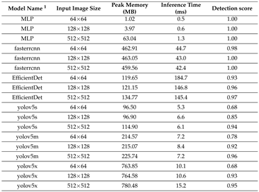
We measured the inference speed and memory usage of the clothing MLP (4-16-16-49), and compared them with those of YOLOv5 (s, m, x), Faster R-CNN, and EfficientDet [33,34,35]. These serve as representative spatial-pattern-based object detectors that are thoroughly studied in the research community, with well-documented reproducibility for measuring inference time and memory use. YOLOv5 provides multiple model sizes, so we evaluated three different ones to examine speed versus performance.
By comparing these methods, we aimed to clarify the advantages of the MLP. Note that we used the default hyperparameters and weights recommended by each official repository (YOLOv5, Faster R-CNN, and EfficientDet). Our MLP had fixed hidden layers of 16 × 2 units. We ran all tests on an NVIDIA TITAN V GPU.
We used images of three different sizes (512×512, 128×128, and 64×64 pixels) as inputs and measured the inference speed for each model (Figure 18). To reconstruct the MLP results, we applied the pixel-level predictions in 2D. Spatial-pattern-based methods often lose performance when a person’s size becomes small. By contrast, because our MLP determines each pixel based on spectral data alone, its performance is less affected by lower image resolution.
Table 8 lists the speed, memory usage, and detection performance for a particular test image. Our MLP used only 63.0 MB for a 512×512 pixel image input and 1.02 MB for a 64×64 input, achieving inference times of 1.3 ms (512×512) to 0.5 ms (64×64). (Figure 19 shows the inference speed, memory usage, and detection score, respectively.) Thus, the MLP is fast, memory-efficient, and robust to changes in spatial resolution.
Because our hyperspectral camera is intended for still images, we did not measure the frames per second (FPS) for a video stream. As shown in Table 8, the MLP processing (inference) requires only 1.3 ms per 512×512 pixel image, and the bounding box processing takes less than 1.0 ms, resulting in a total processing time of approximately 2.3 ms per image. YOLOv5m or YOLOv5s exceed 10 ms. Typically, real-time processing at 30 FPS is achievable if the processing time for each frame is under 33 ms. Therefore, MLP-based inference could theoretically achieve 30 FPS, although the duration of camera data transfer remains uncertain and is left for future work.
All spatial-pattern-based detectors consumed more memory than our MLP. These results confirm that a method exploiting only spectral data can require fewer computational resources. We plan to extend these tests to a multispectral camera supporting the video mode in future work, incorporating sensor frame rates and transfer times to confirm overall real-time feasibility.
(Summary of Section 4)
From the above results:
- MLP classification performance can be better with about 12 bands than with all 167 bands.
- With an optimal choice of bands, performance can be mostly maintained with as few as four bands.
- The method remains relatively robust to small shifts in wavelengths.
Hence, the 4-band OWS, with an F1-score of around 0.95, offers the best balance of detection accuracy, computational lightness, and practical feasibility. In the future, we plan to prototype a 4-band filter for a camera and evaluate its real-time performance outdoors under daylight conditions.
5. Experiments Using Actual Images
We investigated whether clothing could be accurately separated from the background in real images. Because the model performance can vary slightly depending on random factors in the training algorithm, we selected one MLP trained on OWS4-1 that yielded good results on sample images.
5.1. Validity of the 4-Band OWS Model
Figure 20 compares inference results of models using different numbers of bands: MLP-12, OWS5-1, OWS4-1, and OWS3-1. Each result is a pixel-level classification reconstructed as a 2D image, where bright yellow indicates clothing and black indicates background. The clothing on the person was not included in the training data. The scene includes sky, ground, vegetation, cars, signs, and other artificial objects.
Models with five (c) or four (d) bands maintained accuracy comparable to the 12-band model (b), whereas the 3-band model (e) gave more misclassification. Hence, the MLP with the 4-band OWS (d) appears to be effective.
5.2. Generalization to Clothing not Included in the Training
Figure 21(a) shows a pseudo-color image of a street scene containing a person wearing clothing for which the model was not trained. Figure 21(b) presents the pixel-level classification by the 4-band OWS MLP, color-coded by the predicted label. The MLP yields multi-label outputs: black for an inorganic background, dark green for a plant background, and other colors for clothing. The clothing color is determined by whichever label was assigned during training.
Although the jacket is composed of a single material and dye, the detection result merges multiple “clothing labels.” Figure 21 details which labels were recognized. A single garment can appear as multiple clusters of labeled regions—some illuminated by direct sunlight, others in shadow—yet they all belong to “clothing.”
Figure 22 shows various samples of clothing not included in the training. In each case, the clothing was classified under at least one of the learned clothing labels (except for a single case misidentified as “plant”).
5.3. Analysis of Objects That Are Difficult to Detect
Using a range of real-world scenes, we examined which objects might cause errors for this purely spectral-based method. Figure 23 shows an example street scene likely to produce false positives. Figure 24 illustrate clothing likely to be missed. Figure 25 shows clothing materials (genuine leather or synthetic leather) that deviate from this study’s “clothing hypothesis.”
In summary, the following cases are problematic:
- Any object perceived as red or yellow by the human eye, and whose spectrum (extending into the near-infrared) closely matches that of clothing, is prone to being misclassified as clothing, regardless of its material. (Figure 23).
- White wool or black wool and Gray cotton garments may be missed (Figure 24).
- Clothing made of materials that deviate from the “fibers in the hypothesis” (Figure 25), for example, genuine or synthetic leather, may be missed.
Finally, Figure 26 shows various scene examples with predictions by the 4-band OWS4-1 MLP. Panel (a) shows images not used in the training and (b) consists of images used in training. Most unlearned samples are correctly detected as clothing.
6. Discussion
6.1. Effectiveness of Wavelength Selection
The results indicate that, by selecting four wavelengths spanning the visible to near-infrared region, clothing detection is feasible to some extent. Using only four bands instead of the full spectrum simplifies the camera system and offers advantages for real-time capability.
Tests confirmed that using only the visible range or only the near-infrared was insufficient. Employing both visible and near-infrared wavelengths together proved critical. In other words, adding near-infrared to visible bands improved detection performance over visible-only approaches.
6.2. Effectiveness of Each Wavelength
Why are these four specific wavelengths so effective? Here, we consider the physical and spectral background. We hypothesize the roles of the four bands in OWS4-1 as follows:
-
Fourth Wavelength: Capturing “many garments”As shown in Figure 14, the majority of clothing (32 labels) exhibits high reflectance in the 4th wavelength. This band captures the high near-infrared reflectance of most clothing, consistent with our hypothesis that fibers/dyes often reflect well in the near infrared. In addition, combining this band with the second or third bands is helpful for identifying particular clothing colors.
-
Combination of Second, Third, and Fourth Wavelengths: Distinguishing “green/blue clothing” from vegetationThe second and third wavelengths alone do not appear to capture any single specific physical property. We infer that the reflectance pattern across these three bands (including the fourth) helps discriminate certain colors. For instance, the clothes labeled “P-Blue + C-Blue,” “P-Green + C-Green,” “P Sax Blue,” and “P Lt. Green + C Bright Green” have low reflectance at the 4th band. Figure 27(a) shows their 4-band reflectance, all satisfying 2nd band > 3rd band = 4th band. However, the hyperspectral curves in Figure 27(b) reveal that these green/blue garment curves do rise sharply beyond 708 nm. Because the 4th band (708 nm) is slightly short of the near-infrared region where reflection spikes, these garments appear to have lower reflectance at that band.However, vegetation that looks similarly green to the human eye shows 2nd band > 3rd band < 4th band, as indicated by Figure 28. Comparison of Figure 27(b) and Figure 28(b) indicates that vegetation transitions to high near-infrared reflectance at a slightly shorter wavelength than does green clothing. Hence, the 2nd, 3rd, and 4th wavelengths together capture this difference in the onset of near-infrared reflectance, allowing the model to distinguish green clothing from plants.
-
First Wavelength: Capturing “white clothing”In Figure 29, we show (a) the 4-band reflectance and (b) the hyperspectral reflectance of white polyester/cotton garments (“P-White + C-White”). Their reflectance is very high (above 1.0) at the first band, likely due to fluorescent brighteners used in white fabric dyes [36,37,38]. Hence, the first wavelength is effective for capturing the high reflectance of P+C whites. White wool (“W-White”) may likewise incorporate fluorescent brighteners, as evidenced by a peak at approximately 440 nm in the 167-band data. However, the peak wavelength of these brighteners ( nm) inferred from the spectral curves does not fully coincide with the first wavelength (453 nm). This discrepancy suggests that the convergence approach employed in this study will benefit from further refinement.
6.3. Limitations of Spectral-Only Detection: Counterexamples of Hypothesis, Materials, Nighttime, and Red/Yellow
- Counterexamples to the Hypothesis:Uncolored wool or gray cotton that does not increase near-infrared reflectance is easily missed. Nude bodies are not considered.
- Material Constraints:Leather or synthetic leather that does not reflect well in the near-infrared cannot be detected. Military camouflage clothing [39] or materials that are difficult to see even with the naked eye are beyond the scope of this method.
- Nighttime or Low-Light Environments:Our experiments assume outdoor daytime conditions. Nighttime use would require external infrared illumination. Because spectral distributions change drastically under different lighting, our approach cannot be directly applied.
- Red or Yellow Background: If these colors have spectral properties similar to that of clothing, false positives may occur.
Possible countermeasures include (1) collecting extra training data emphasizing these challenging garments, or (2) introducing a hybrid method that combines spectral data with spatial pattern features such as texture or shape. However, adding more challenging clothing might also increase false positives for similar backgrounds. Also, incorporating spatial pattern recognition can increase the computational demand, undermining the speed advantages of a purely spectral approach.
Hence, we consider it reasonable to “give up” in cases where the material does not satisfy the “fiber high near-infrared reflectance” assumption or where background objects share very similar spectra. In this research, we deliberately focused on the scenario of daytime outdoor people wearing normal fiber garments, which yields high recall within that domain.
To our knowledge, there is no clear statistical data confirming that most people in public areas wear textile garments, but in urban environments, this is generally true. Therefore, treating clothing detection as an approximation of human detection is likely to have sufficient merit.
6.4. Prospects for MLP Model Generalization
The dataset of hyperspectral images used in this study was limited, covering only daytime outdoor environments and a modest number of test images. Nighttime or highly dynamic situations have not been evaluated. Even so, the real-image results in Section 5 suggest some degree of generalization: the model detected clothing that was not part of the training.
Going forward, we must clarify the range of scenarios for which the “clothing hypothesis” is valid. A much larger dataset spanning various locations, times, weather conditions, and urban/rural settings will be needed to further assess the generality of clothing detection. With sufficient data from large-scale experiments, we can gain deeper insight into how broadly the method applies.
Because a still-image hyperspectral camera makes large-scale data collection difficult, we plan to use a smaller, video-capable spectral camera to capture diverse scenes and subjects continuously, thus enriching the training data.
6.5. Outlook for a Real-Time Camera System
The MLP approach offers fast, memory-efficient inference, suitable for IoT devices or compact cameras. Using only four bands reduces the complexity compared to high-end systems with many bands. From the robustness evaluation in Section 4-3-3, we can see that moderate variations in the center wavelength or passband width are tolerable, making it feasible to use off-the-shelf filters.
Small multispectral cameras with selectable wavelengths, such as polarization-based multispectral cameras [40] or multi-lens TOMBO cameras [41,42,43], can potentially be adapted to create a 4-band camera for human detection. In outdoor settings, however, illumination can vary by time and place, so we must address how to track or adapt to changing lighting conditions.
We plan to move forward with prototyping. Adapting to nighttime or indoor settings through infrared illumination or an improved sensor signal-to-noise ratio is a future challenge.
7. Conclusions
This study has demonstrated the effectiveness of a human detection technique that leverages the spectral properties of clothing. The following three points summarize the main conclusions:
-
Detection Performance in Daytime Outdoor ConditionsBy exploiting the spectral reflectance from visible to near-infrared wavelengths, we confirmed stable clothing detection in daytime outdoor environments.
-
Efficient Detection by Selecting Four WavelengthsEven without using the entire spectrum, accuracy as high as an F1-score of around 0.95 can be achieved by only four wavelengths, specifically 453, 556, 668, and 708 nm. This indicates strong practical potential, balancing a simple setup with fast processing.
-
Limitations of Purely Spectral DetectionObjects with similar spectra, such as red or yellow objects, white wool, or gray cotton, pose a risk of false positives or missed detections. Where spectral methods alone fail, one must consider spatial pattern recognition, which, however, can undermine the speed and computational lightness of this approach.
Our method holds promise in scenarios requiring real-time human detection, such as security cameras, autonomous driving, and disaster rescue. It may also simplify camera systems and has potential for both research and real-world solutions. In the future, once a real-time camera system is developed, larger video-based datasets can be collected under diverse backgrounds, which may further expand the robustness and performance of the method.
Funding
This research received no external funding.
Institutional Review Board Statement
Not applicable.
Informed Consent Statement
Not applicable.
Data Availability Statement
Due to corporate confidentiality and proprietary considerations, the datasets generated and/or analyzed during the current study are not publicly available. However, summary statistics and non-sensitive aggregated results are available from the corresponding author upon reasonable request.
Conflicts of Interest
The authors declare no conflict of interest.
References
- Textile Exchange. Preferred Fiber & Materials Market Report 2022. 2022. https://textileexchange.org/knowledge-center/reports/materials-market-report-2022/. (accessed on 27 January 2025).
- Girshick, R.; Donahue, J.; Darrell, T.; Malik, J. Rich feature hierarchies for accurate object detection and semantic segmentation. In Proceedings of the Proceedings of the IEEE Conference on Computer Vision and Pattern Recognition, 2014, pp.580–587. [CrossRef]
- Redmon, J.; Divvala, S.; Girshick, R.; Farhadi, A. You only look once: Unified, real-time object detection. In Proceedings of the Proceedings of the IEEE Conference on Computer Vision and Pattern Recognition, 2016, pp.779–788. [CrossRef]
- Liu, W.; Anguelov, D.; Erhan, D.; Szegedy, C.; Reed, S.; Fu, C.Y.; Berg, A.C. SSD: Single shot multibox detector. In Proceedings of the European Conference on Computer Vision; 2016; pp. 21–37. [Google Scholar] [CrossRef]
- Ren, S.; He, K.; Girshick, R.; Sun, J. Faster R-CNN: Towards real-time object detection with region proposal networks. IEEE Transactions on Pattern Analysis and Machine Intelligence 2017, 39, 1137–1149. [Google Scholar] [CrossRef] [PubMed]
- Zhu, C.; He, Y.; Savvides, M. Feature selective anchor-free module for single-shot object detection. In Proceedings of the Proceedings of the IEEE Conference on Computer Vision and Pattern Recognition, 2019, pp.840–849. [CrossRef]
- Hwang, S.; Kim, J.; Park, S.; Kim, N.; Yoon, K.J. Multispectral Pedestrian Detection: Benchmark Dataset and Baseline. In Proceedings of the Proceedings of the IEEE Conference on Computer Vision and Pattern Recognition (CVPR), 2015, pp.1037–1045. [CrossRef]
- González, D.; Fang, Z.; Sancho-Pelluz, T.; De la Torre, F. Pedestrian Detection at Day/Night Time with Visible and FIR Cameras. Sensors 2016, 16, 820. [Google Scholar] [CrossRef]
- Li, X.; Zhang, S.; Wang, T.; Lin, L.; Li, B.; Yang, M.H. Illumination-Aware Faster R-CNN for Robust Multispectral Pedestrian Detection. Pattern Recognition 2019, 85, 161–171. [Google Scholar] [CrossRef]
- Winkens, T.; Pfeiffer, D.; Franke, U. HyKo: A Spectral Dataset for Scene Understanding. In Proceedings of the Proceedings of the ICCV 2017 Workshops, 2017, pp.94–99.
- Basterretxea, K.; Martínez, V.; Echanobe, J.; Gutiérrez-Zaballa, J.; del Campo, I. HSI-Drive: A Dataset for the Research of Hyperspectral Image Processing Applied to Autonomous Driving Systems. Proceedings of the IEEE Intelligent Vehicles Symposium 2021, 2021, 957–5298. [Google Scholar] [CrossRef]
- Basterretxea, K.; Martínez, V.; Echanobe, J.; Gutiérrez-Zaballa, J.; del Campo, I. HSI-Drive v2.0: More Data for New Challenges in Scene Understanding. arXiv preprint, 2023; arXiv:2411.17530. [Google Scholar]
- Zhang, Y.; Zhao, Y.; Wu, Y.; et al. Hyperspectral Imaging-Based Perception in Autonomous Driving Scenarios: Benchmarking Baseline Semantic Segmentation Models. arXiv preprint arXiv:2410.22101, arXiv:2410.22101 2024.
- Kosugi, Y.; Murase, T.; Asano, T.; Uto, A.; Takagishi, S.; Moriguchi, M. Sensing On-road Objects by Infrared Hyper Spectrum. SEI Technical Review 2010, 176, 27–32. [Google Scholar]
- Scientific, T.F. Utilizing UV-Visible Spectroscopy for Color Analysis of Fabrics. 2024. https://assets.thermofisher.com/TFS-Assets/CAD/Application-Notes/color-analysis-of-fabric-app-note-1529047.pdf. (accessed on 28 January 2025).
- Jamieson, K.; Talwalkar, A. Non-stochastic best arm identification and hyperparameter optimization. In Proceedings of the Artificial Intelligence and Statistics (AISTATS); 2016; pp. 240–248. [Google Scholar]
- Li, L.; Jamieson, K.; DeSalvo, G.; Rostamizadeh, A.; Talwalkar, A. Hyperband: A novel bandit-based approach to hyperparameter optimization. Journal of Machine Learning Research 2018, 18, 1–52. [Google Scholar]
- Savitzky, A.; Golay, M.J.E. Smoothing and differentiation of data by simplified least squares procedures. Analytical Chemistry 1964, 36, 1627–1639. [Google Scholar] [CrossRef]
- Tucker, C.J. Red and photographic infrared linear combinations for monitoring vegetation. Remote Sensing of Environment 1979, 8, 127–150. [Google Scholar] [CrossRef]
- Pedregosa, F.; Varoquaux, G.; Gramfort, A.; Michel, V.; Thirion, B.; Grisel, O.; Blondel, M.; Prettenhofer, P.; Weiss, R.; Dubourg, V.; et al. Scikit-learn: Machine Learning in Python. Journal of Machine Learning Research 2011, 12, 2825–2830. [Google Scholar]
- Cortes, C.; Vapnik, V. Support-vector networks. Machine Learning 1995, 20, 273–297. [Google Scholar] [CrossRef]
- Breiman, L. Random forests. Machine Learning 2001, 45, 5–32. [Google Scholar] [CrossRef]
- Friedman, J.H. Greedy function approximation: A gradient boosting machine. Annals of Statistics 2001, 29, 1189–1232. [Google Scholar] [CrossRef]
- Freund, Y.; Schapire, R.E. A short introduction to boosting. Journal of the Japanese Society for Artificial Intelligence 1999, 14, 1612. [Google Scholar] [CrossRef]
- Rumelhart, D.E.; Hinton, G.E.; Williams, R.J. Learning representations by back-propagating errors. Nature 1986, 323, 533–536. [Google Scholar] [CrossRef]
- Bellman, R. On Adaptive Control Processes. IRE Transactions on Automatic Control 1956, 4, 1–9. [Google Scholar] [CrossRef]
- Chang, C.I.; Du, Q.; Sun, T.S.; Althouse, M.L. A joint band prioritization and band-decorrelation approach to band selection for hyperspectral image classification. IEEE Transactions on Geoscience and Remote Sensing 1999, 37, 2631–2641. [Google Scholar] [CrossRef]
- Falkner, S.; Klein, A.; Hutter, F. BOHB: Robust and efficient hyperparameter optimization at scale. In Proceedings of the International Conference on Machine Learning (ICML); 2018; pp. 1437–1446. [Google Scholar]
- Li, L.; Jamieson, K.; Rostamizadeh, A.; Gonina, K.; Hardt, M.; Recht, B.; Talwalkar, A. A system for massively parallel hyperparameter tuning. In Proceedings of the Proceedings of Machine Learning and Systems, 2020, pp.230–246.
- SA, P. Parrot Sequoia Multispectral Sensor. https://www.parrot.com/us/, 2015. Accessed: 2025-02-15.
- DJI. Phantom 4 Multispectral. https://ag.dji.com/jp?site=brandsite&from=nav, 2019. Accessed: 2025-02-15.
- MicaSense, I. RedEdge-MX Multispectral Sensor. https://www.micasense.com/rededge-mx/, 2018. Accessed: 2025-02-15.
- Jocher, G.; et al. ultralytics/yolov5: V3.0. Zenodo, 2020. https://github.com/ultralytics/yolov5. [CrossRef]
- Ren, S.; He, K.; Girshick, R.; Sun, J. Faster R-CNN: Towards real-time object detection with region proposal networks. In Proceedings of the Advances in Neural Information Processing Systems (NeurIPS); 2015; pp. 91–99. [Google Scholar]
- Tan, M.; Pang, R.; Le, Q.V. EfficientDet: Scalable and efficient object detection. In Proceedings of the Proceedings of the IEEE/CVF Conference on Computer Vision and Pattern Recognition (CVPR), 2020, pp.
- White, R.H. Mode of Action of Fluorescent Whitening Agents and Measurement of Their Effects. Journal of the Optical Society of America 1957, 47, 933–937. [Google Scholar] [CrossRef]
- Amirshahi, S.H.; Agahian, F. Basis Functions of the Total Radiance Factor of Fluorescent Whitening Agents. Textile Research Journal 2006, 76, 197–207. [Google Scholar] [CrossRef]
- Hassan, M.M.; Islam, M.A.; Hannan, M.A.; Islam, M.S. Influence of Optical Brightening Agent Concentration on Properties of Cotton Knitted Fabric. Polymers 2019, 11, 1919. [Google Scholar] [CrossRef]
- Degenstein, L.M.; Sameoto, D.; Hogan, J.D.; Asad, A.; Dolez, P.I. Smart Textiles for Visible and IR Camouflage Application: State-of-the-Art and Microfabrication Path Forward. Micromachines 2021, 12, 773. [Google Scholar] [CrossRef]
- Ono, S. Snapshot multispectral imaging using a pixel-wise polarization color image sensor. Optics Express 2020, 28, 34536–34573. [Google Scholar] [CrossRef] [PubMed]
- Tanida, J.; Kumagai, T.; Yamada, K.; Miyatake, S.; Ishida, K.; Morimoto, T.; Kondou, N.; Miyazaki, D.; Ichioka, Y. Thin Observation Module by Bound Optics (TOMBO): Concept and Experimental Verification. Applied Optics 2001, 40, 1806–1813. [Google Scholar] [CrossRef] [PubMed]
- Tanida, J.; Miyamoto, Y.; Ishida, M.; Yamada, K.; Kumagai, T.; Miyatake, S.; Ichioka, Y. Multispectral Imaging Using Compact Compound Optics. Optics Express 2004, 12, 1643–1655. [Google Scholar] [CrossRef]
- Nakanishi, T.; Kagawa, K.; Masaki, Y.; Tanida, J. Development of a Mobile TOMBO System for Multi-Spectral Imaging. In Proceedings of the Proceedings of SPIE, the International Society for Optical Engineering, 2020, Vol. [CrossRef]
Figure 1.
Hyperspectral imaging of clothing and scenery. (a) Hyperspectral capture. (b) Examples of clothing images (excerpt). (c) Examples of background images (excerpt).
Figure 1.
Hyperspectral imaging of clothing and scenery. (a) Hyperspectral capture. (b) Examples of clothing images (excerpt). (c) Examples of background images (excerpt).
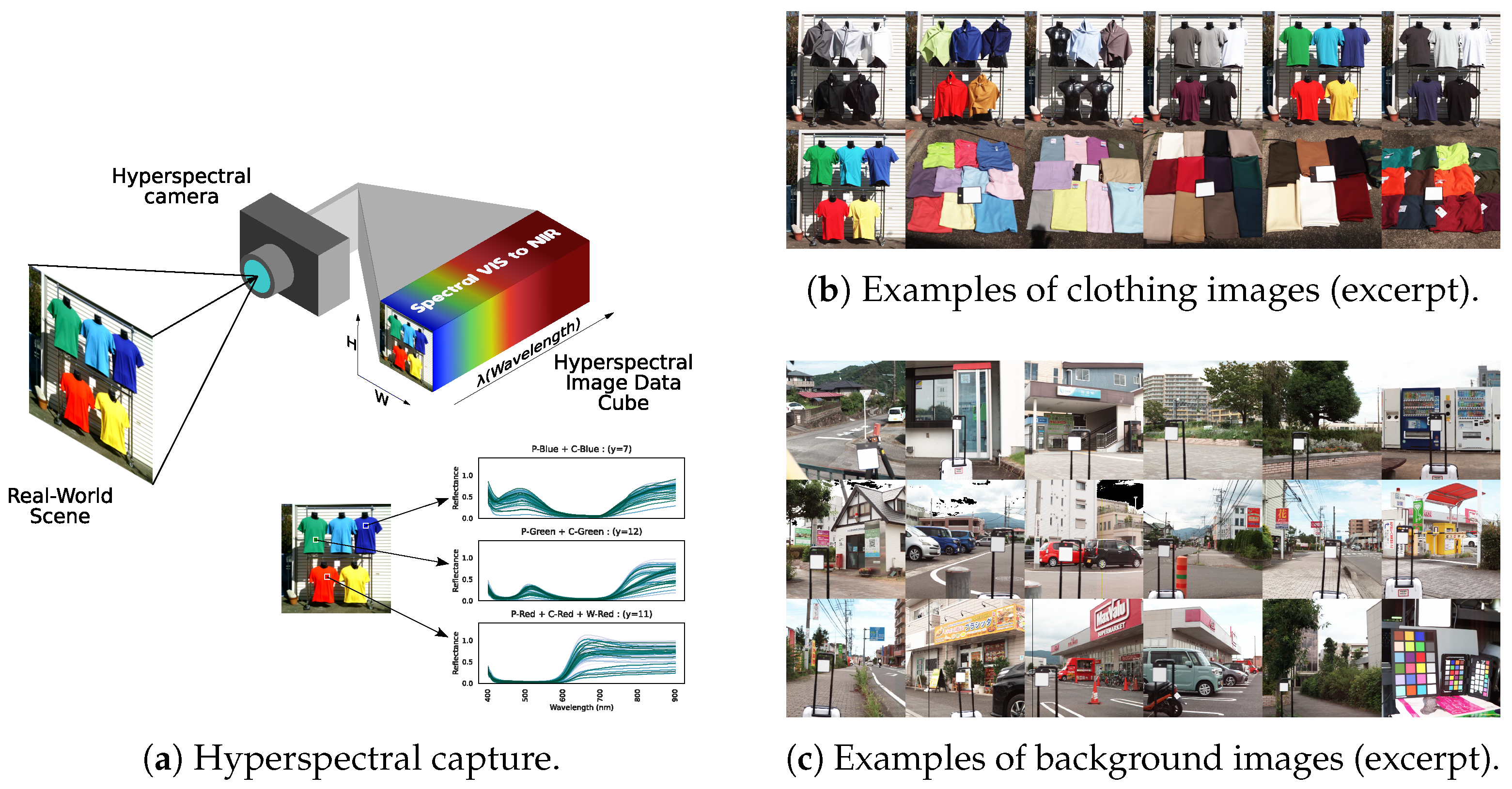
Figure 2.
Example of a labeled image (a) and its corresponding pseudo-color image (b).
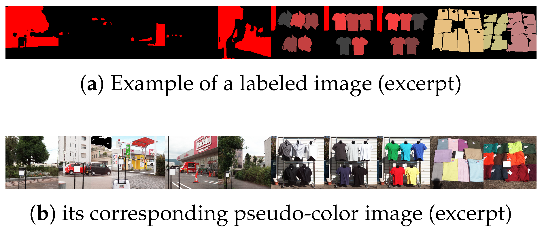
Figure 3.
Hyperspectral reflectance curves, showing reflectance (vertical axis) over the visible–near-infrared range (horizontal axis) for 100 samples. (a) Clothing. (b) Inorganic background. (c) Plant background.
Figure 3.
Hyperspectral reflectance curves, showing reflectance (vertical axis) over the visible–near-infrared range (horizontal axis) for 100 samples. (a) Clothing. (b) Inorganic background. (c) Plant background.
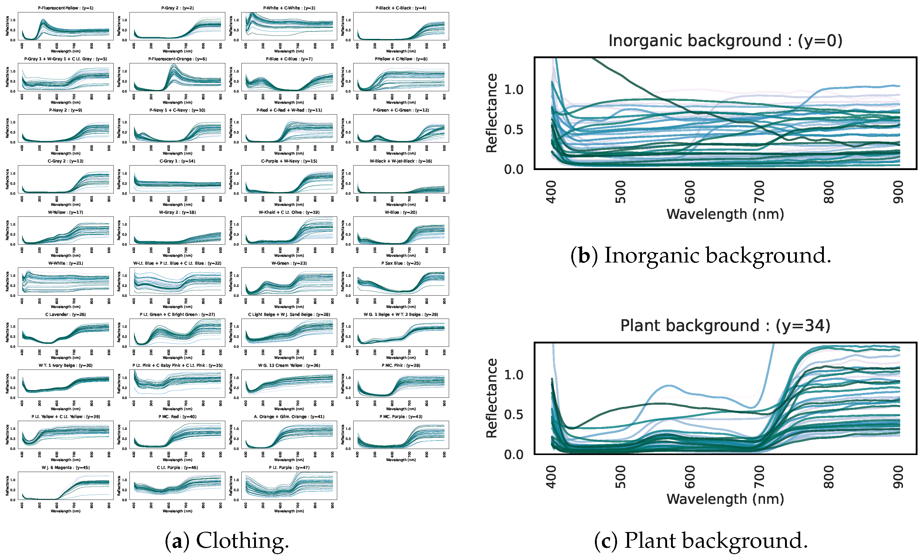
Figure 4.
Multi-Layer Perceptron dataset creation workflow.
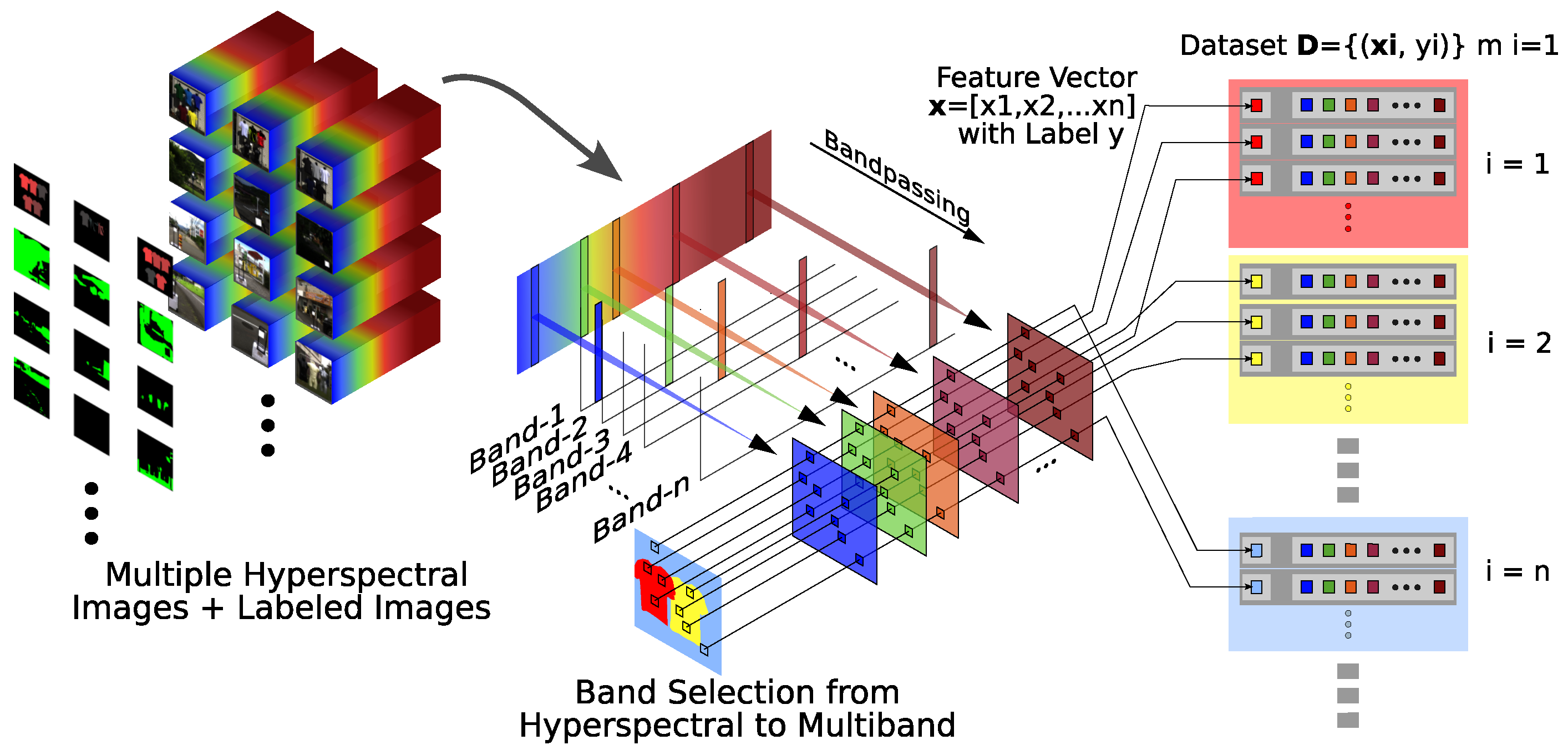
Figure 5.
Sampling example, with moss-green dots indicating chosen pixels.
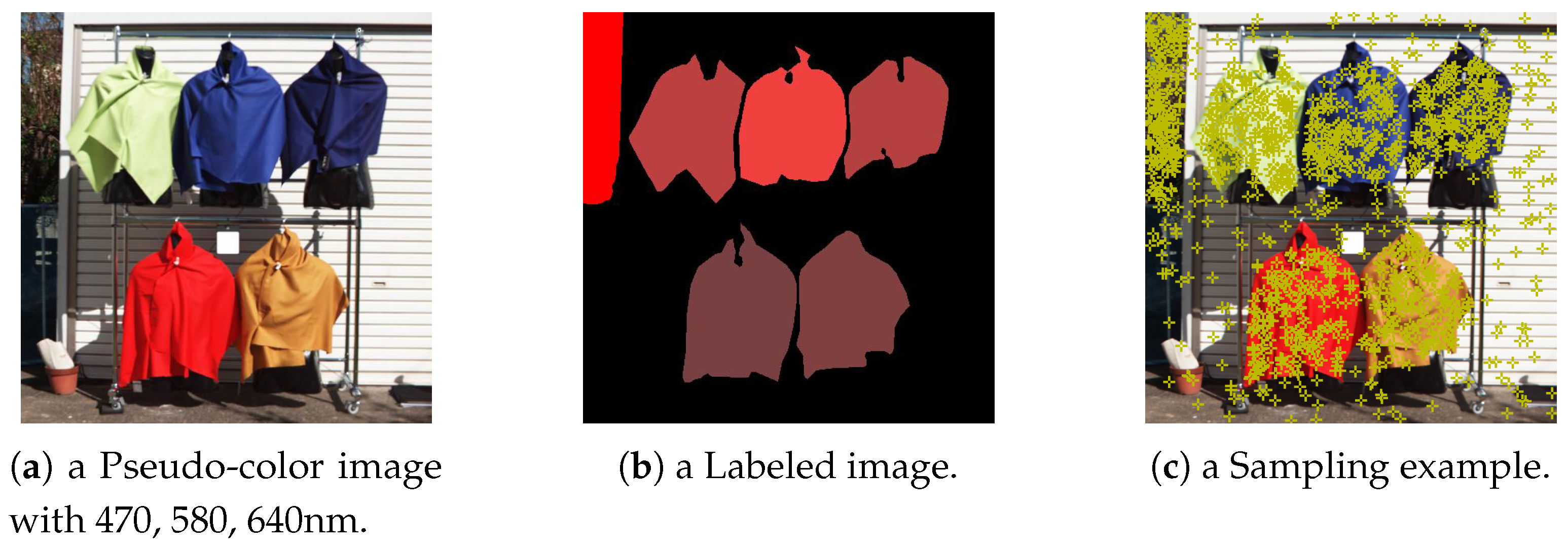
Figure 6.
Multi-Layer Perceptron workflow and multi-label confusion matrix for 167 bands.
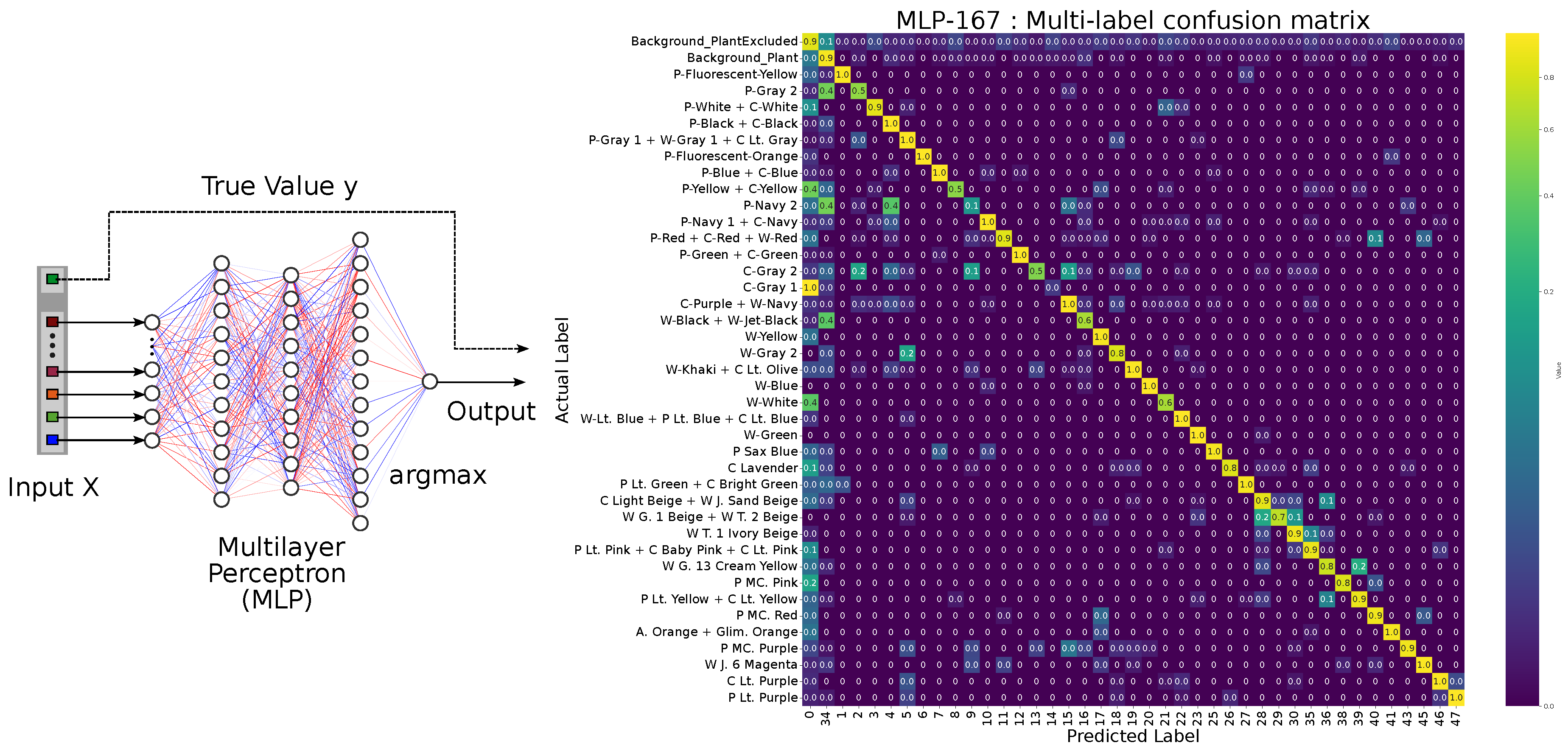
Figure 7.
(a) Conversion to the clothing versus background matrix. (b) Example of the 2×2 confusion matrix for the 167-band model.
Figure 7.
(a) Conversion to the clothing versus background matrix. (b) Example of the 2×2 confusion matrix for the 167-band model.
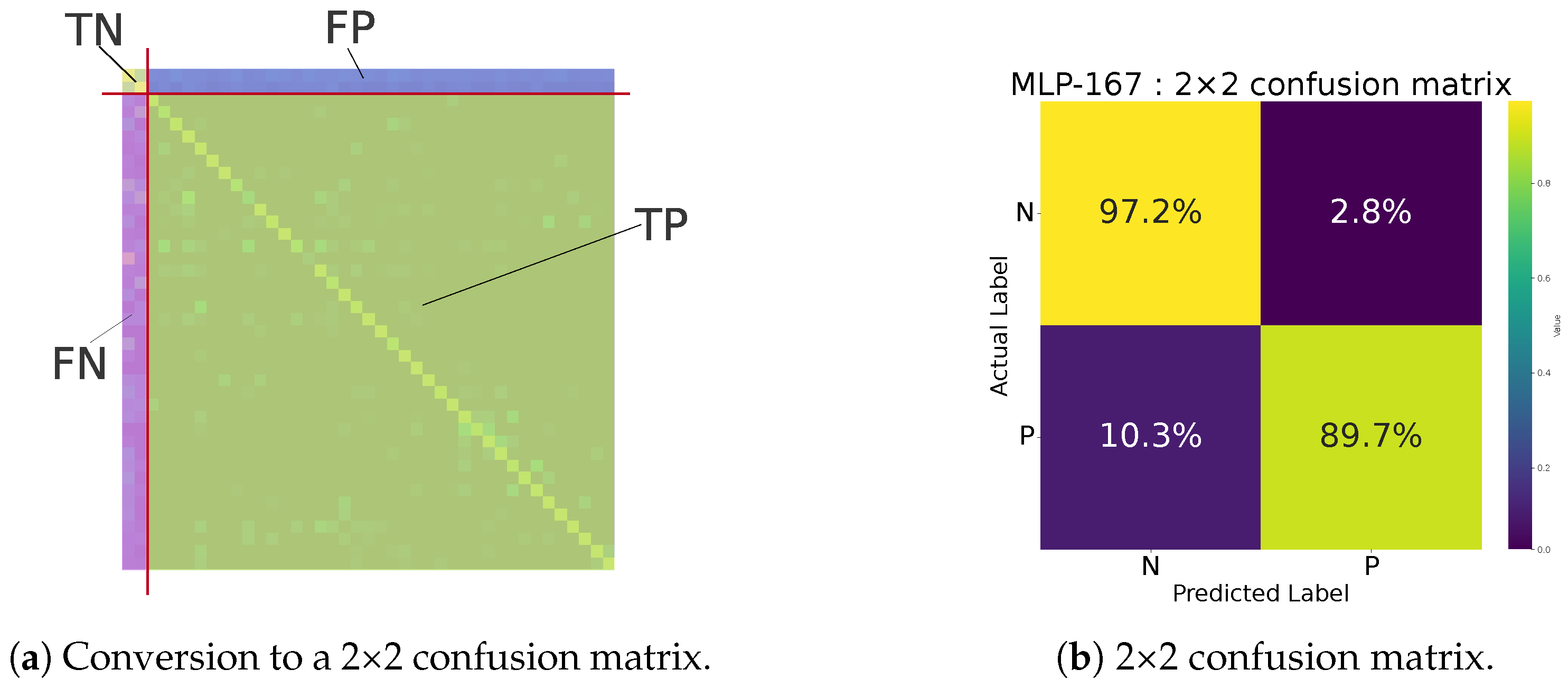
Figure 8.
(a) Multi-label confusion matrix for 12-band Multi-Layer Perceptron (MLP-12). (b) 2×2 confusion matrix for MLP-12.
Figure 8.
(a) Multi-label confusion matrix for 12-band Multi-Layer Perceptron (MLP-12). (b) 2×2 confusion matrix for MLP-12.
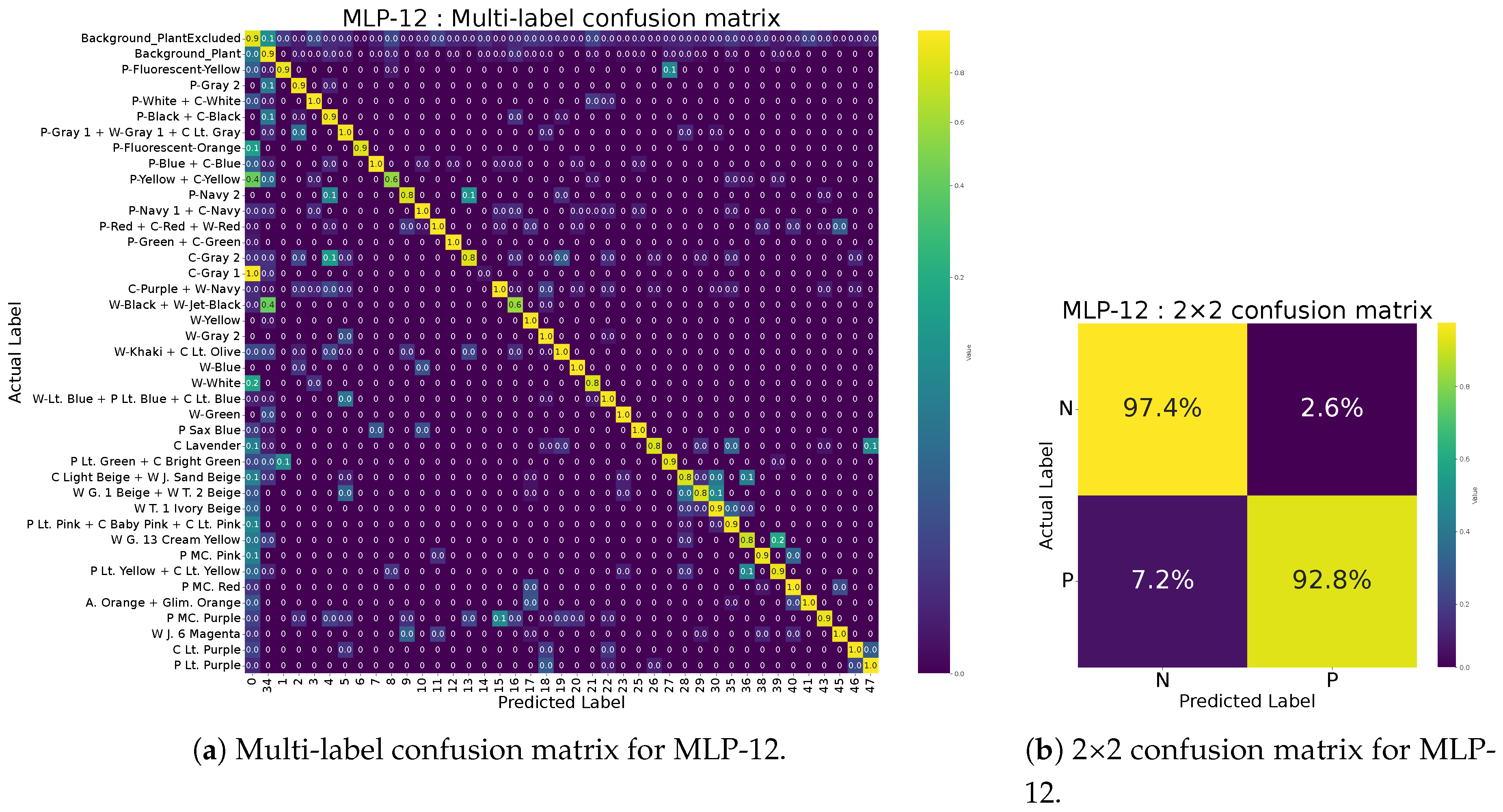
Figure 9.
Relationship between band count and macro_avg.
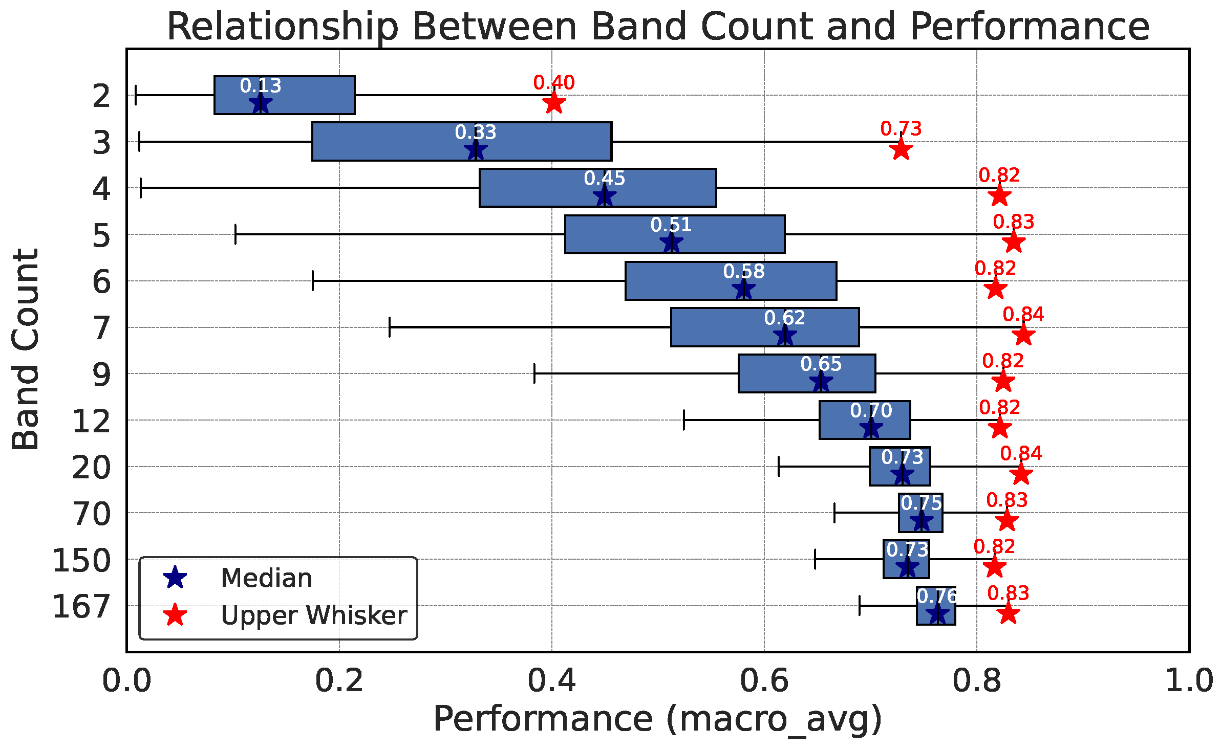
Figure 10.
Flowchart of Optimal Wavelength Set exploration (Steps 1–5 in the text). See Section 4.3.2 for details.
Figure 10.
Flowchart of Optimal Wavelength Set exploration (Steps 1–5 in the text). See Section 4.3.2 for details.
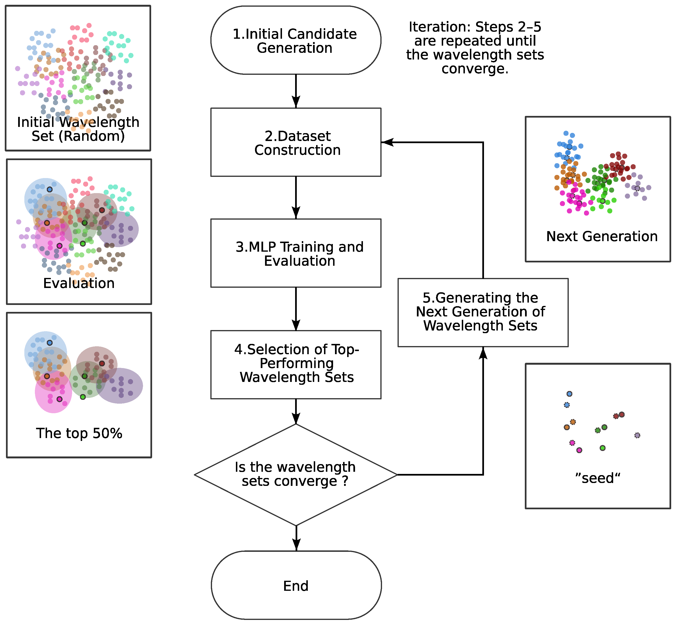
Figure 11.
Example of convergence for the 4-band Optimal Wavelength Set search (from left to right: initial state, iteration 1, iteration 2, iteration 5). (a) Principal Component Analysis (PCA) visualization of wave-set clusters. (b) Deviation (nm) of each band from the mean. The x-axis is the band index (1–4), and the y-axis is the offset in nm.
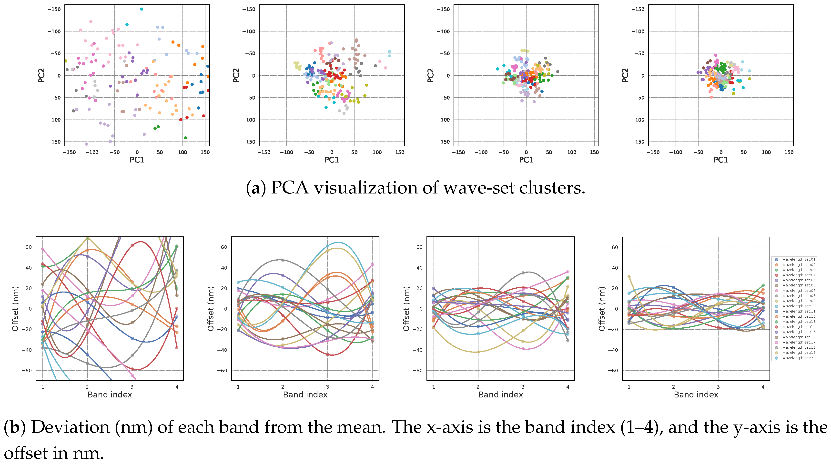
Figure 12.
(a) Multi-label confusion matrix for Optimal Wavelength Set with 4 bands (OWS4-1). (b) 2×2 confusion matrix for OWS4-1.
Figure 12.
(a) Multi-label confusion matrix for Optimal Wavelength Set with 4 bands (OWS4-1). (b) 2×2 confusion matrix for OWS4-1.
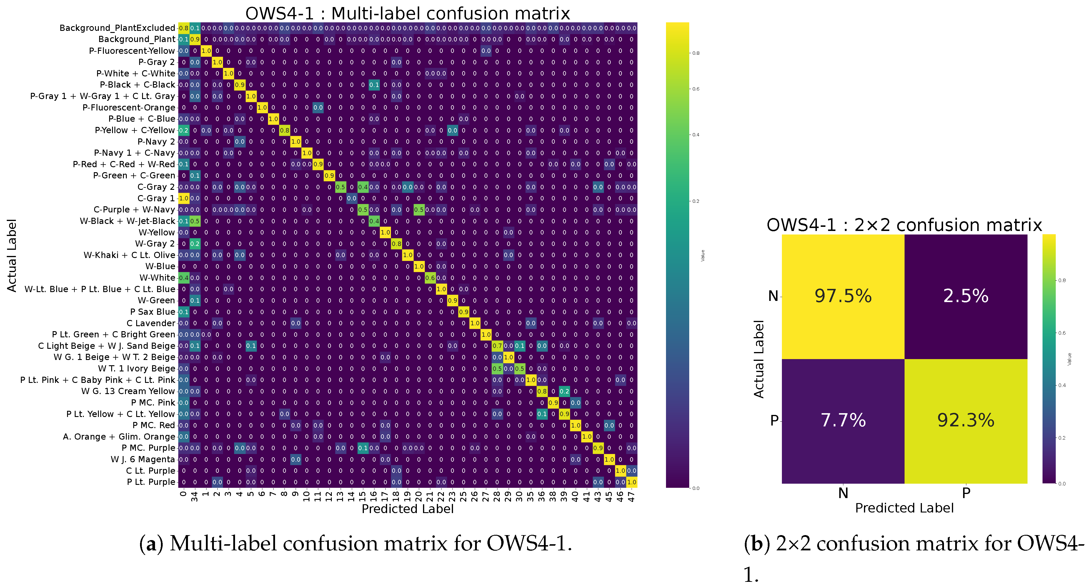
Figure 13.
Passbands of the 4- and 5-band Optimal Wavelength Sets (OWS). (a) OWS4-1. (b) OWS5-1. (c) OWS4-2. (d) OWS5-2.
Figure 13.
Passbands of the 4- and 5-band Optimal Wavelength Sets (OWS). (a) OWS4-1. (b) OWS5-1. (c) OWS4-2. (d) OWS5-2.
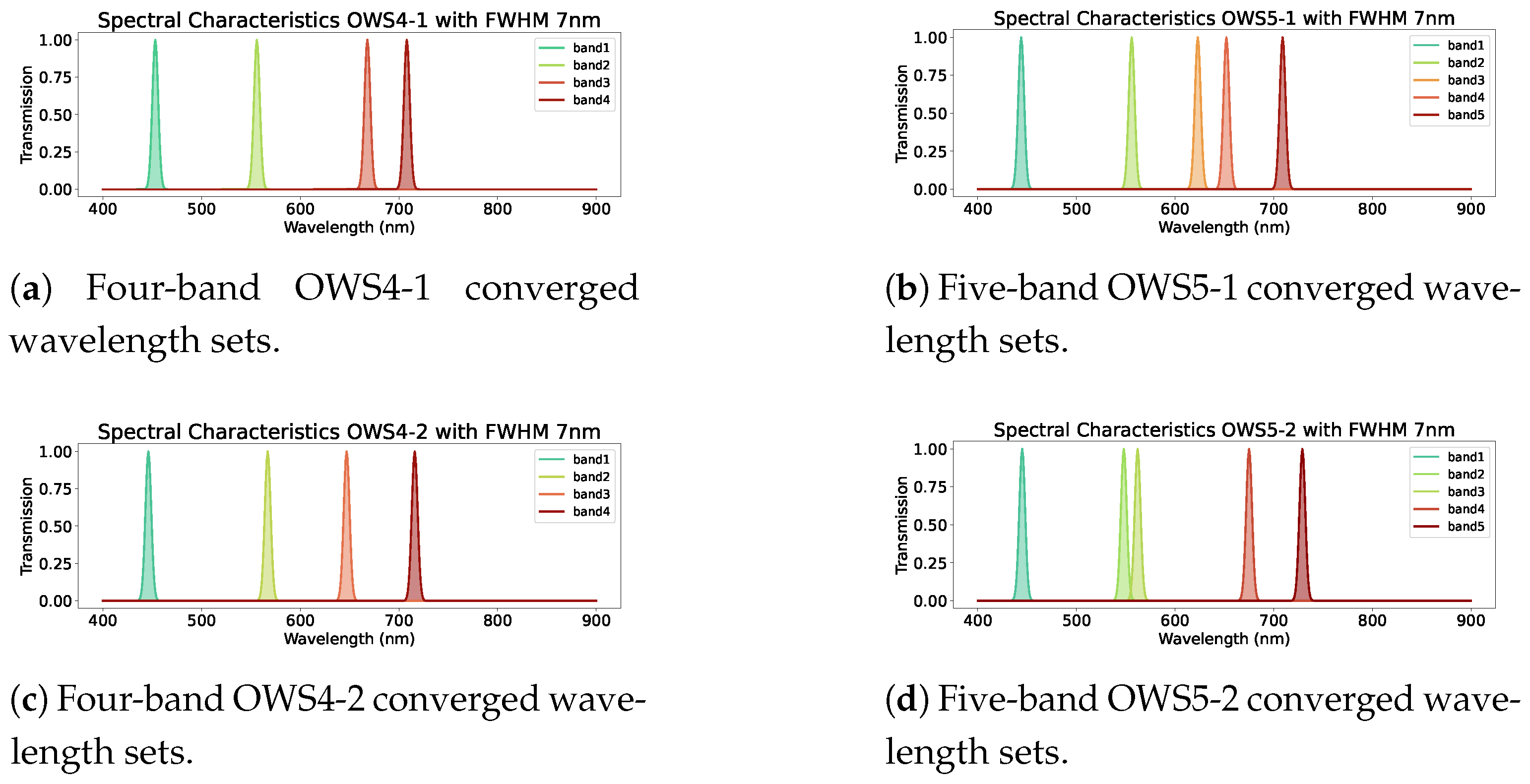
Figure 14.
Multispectral reflectance at the four wavelengths of the Optimal Wavelength Set (OWS4-1: 453, 556, 668, 708 nm) for (a) clothing, (b) inorganic background, and (c) plant background.
Figure 14.
Multispectral reflectance at the four wavelengths of the Optimal Wavelength Set (OWS4-1: 453, 556, 668, 708 nm) for (a) clothing, (b) inorganic background, and (c) plant background.
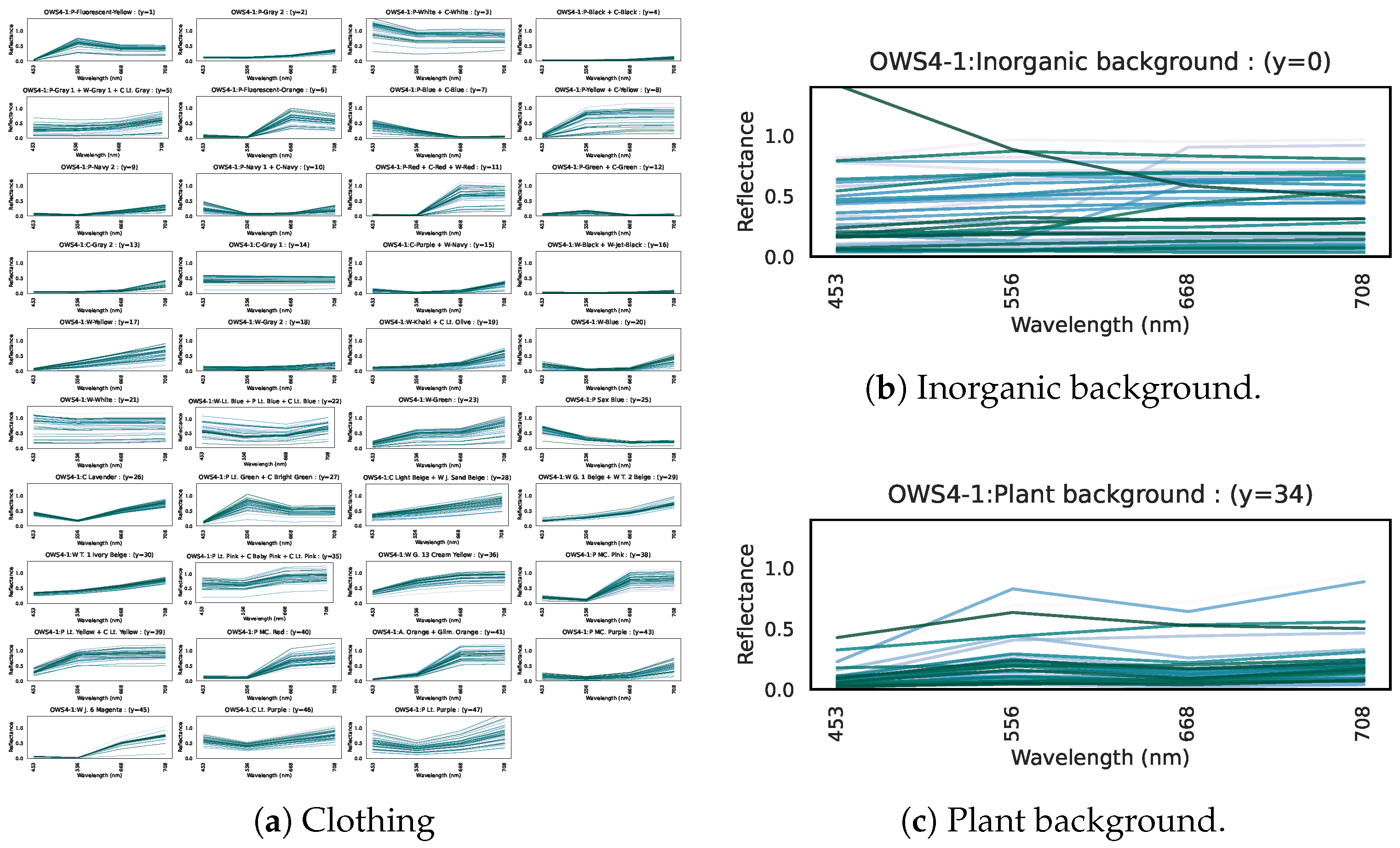
Figure 15.
Performance variation when shifting the center wavelength of each of the 4 bands.
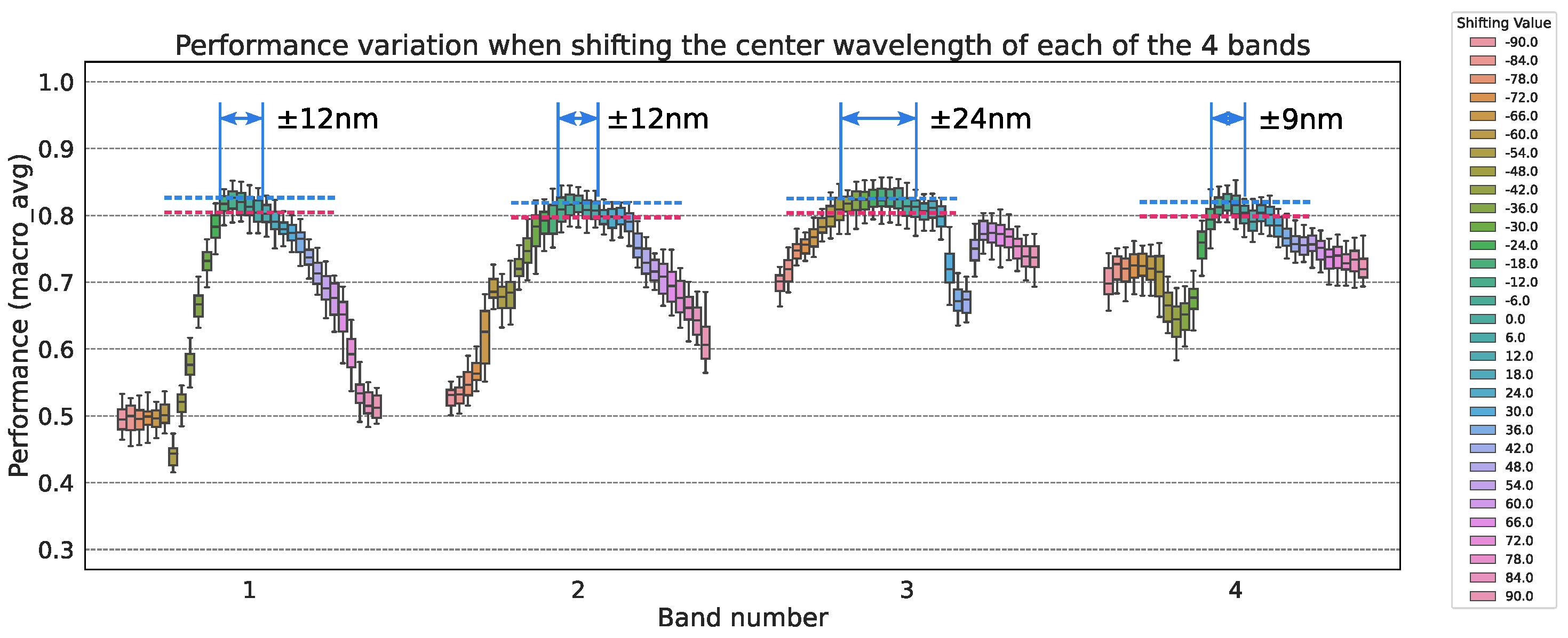
Figure 16.
Performance variation for the 5-band set under center-wavelength shifts. Shifting the 3rd or 4th band alone had minimal impact (see text).
Figure 16.
Performance variation for the 5-band set under center-wavelength shifts. Shifting the 3rd or 4th band alone had minimal impact (see text).
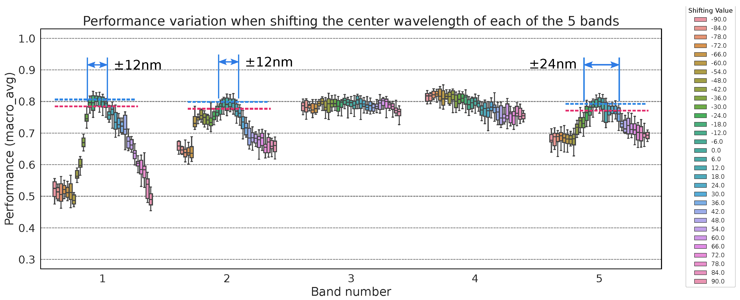
Figure 17.
Performance variation when simultaneously widening the passband of all 4 bands.
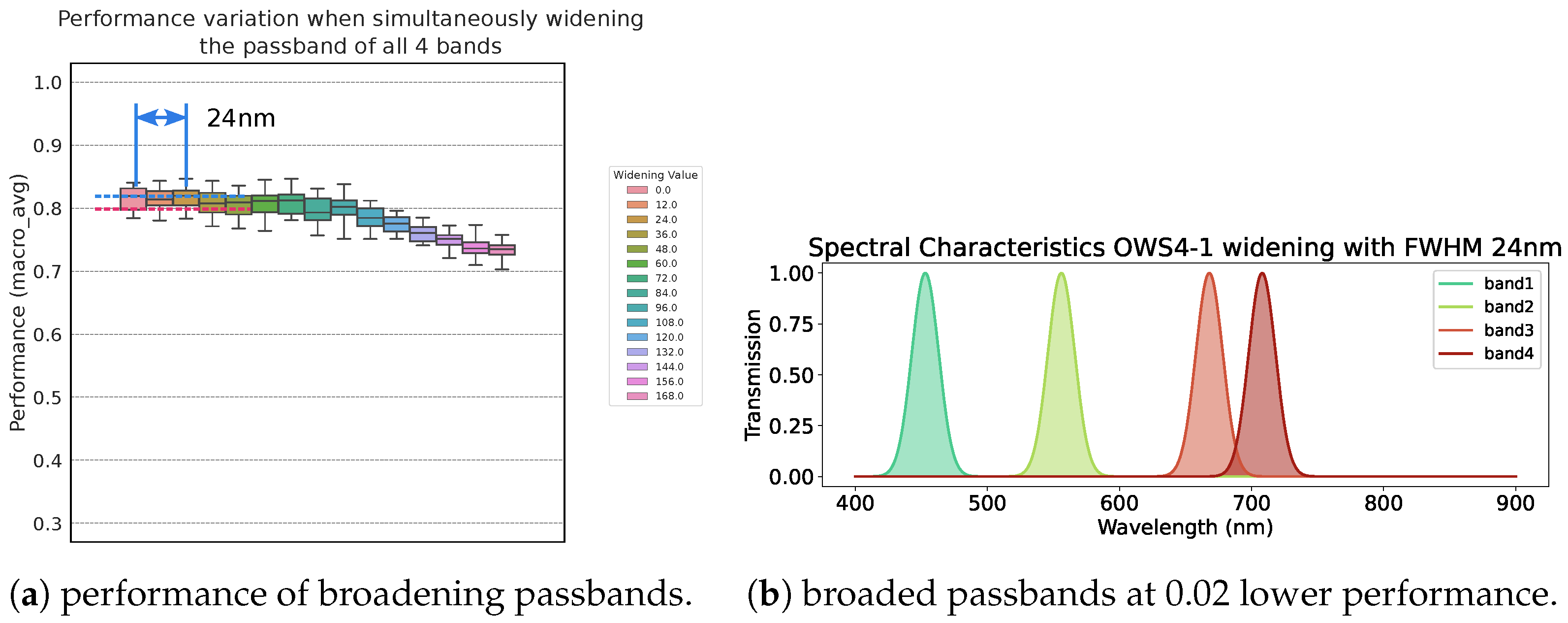
Figure 18.
Example inference results at resolutions (a) Multi-Layer Perceptron (MLP) at 512×512 pixels, (b) MLP at 64×64 pixels, and (c) YOLOv5m at 512×512 pixels, (d) YOLOv5m at 64×64 pixels. The MLP detects the boundary of clothing pixels and draws bounding boxes. It uses only spectral information from each pixel to decide whether it is clothing.
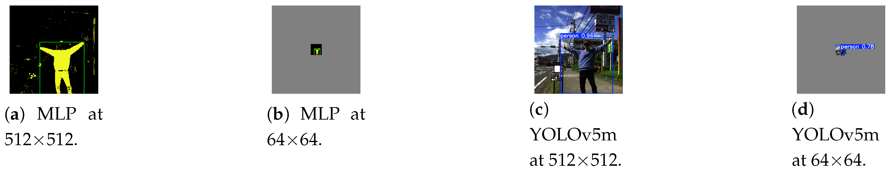
Figure 19.
inference speed, memory usage, and detection score. (a) Inference speed. The Multi-Layer Perceptron (MLP) stays well below the 33 ms real-time threshold. (b) Memory usage. (c) Detection score.
Figure 19.
inference speed, memory usage, and detection score. (a) Inference speed. The Multi-Layer Perceptron (MLP) stays well below the 33 ms real-time threshold. (b) Memory usage. (c) Detection score.
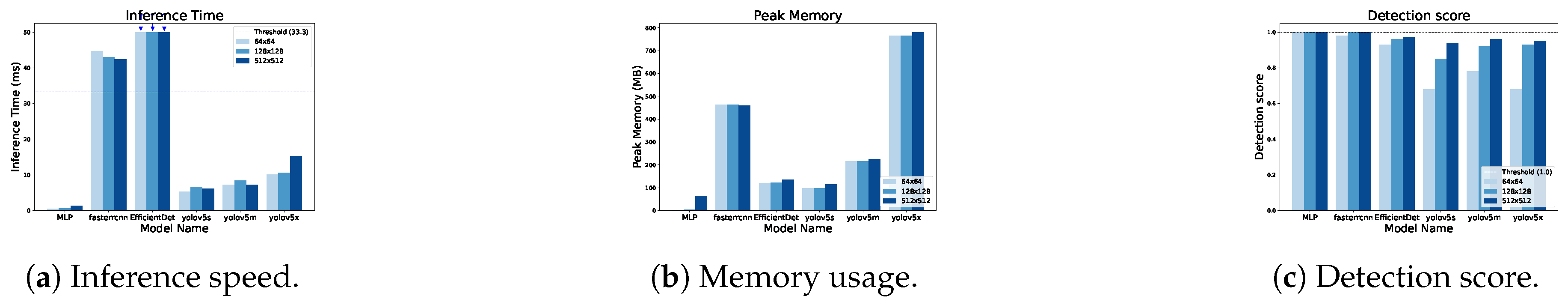
Figure 20.
Examples of inference results from some Wavelength Sets models with different band counts (12, 5, 4, and 3). Models with bands perform well. (a) Pseudo-color image. (b) 12-band Multi-Layer Perceptron (MLP-12). (c) 5-band Optimal Wavelength Set (OWS5-1) MLP. (d) 4-band OWS4-1 MLP. (e) 3-band OWS3-1 MLP.
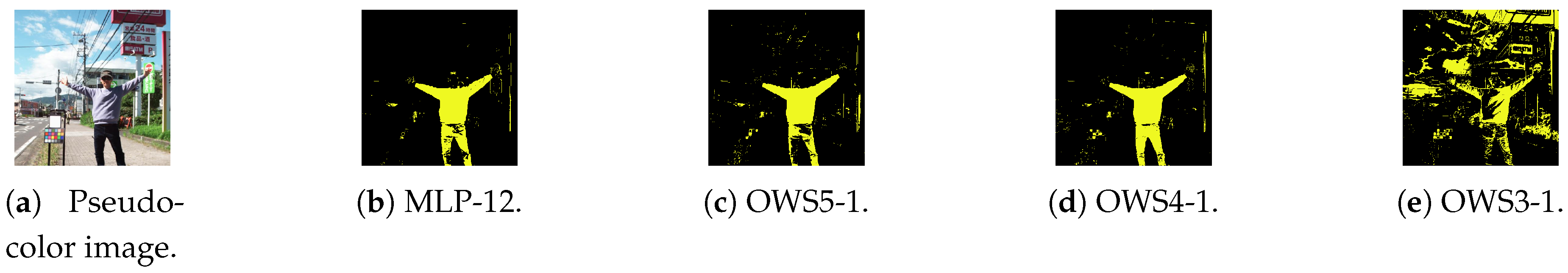
Figure 21.
Example of a street scene containing a person with clothing not included in the training dataset. (a) Pseudo-color image. (b) 4-band Optimal Wavelength Set (OWS4-1) MLP predictions. (c) Detailed labeling of the clothing region.
Figure 21.
Example of a street scene containing a person with clothing not included in the training dataset. (a) Pseudo-color image. (b) 4-band Optimal Wavelength Set (OWS4-1) MLP predictions. (c) Detailed labeling of the clothing region.
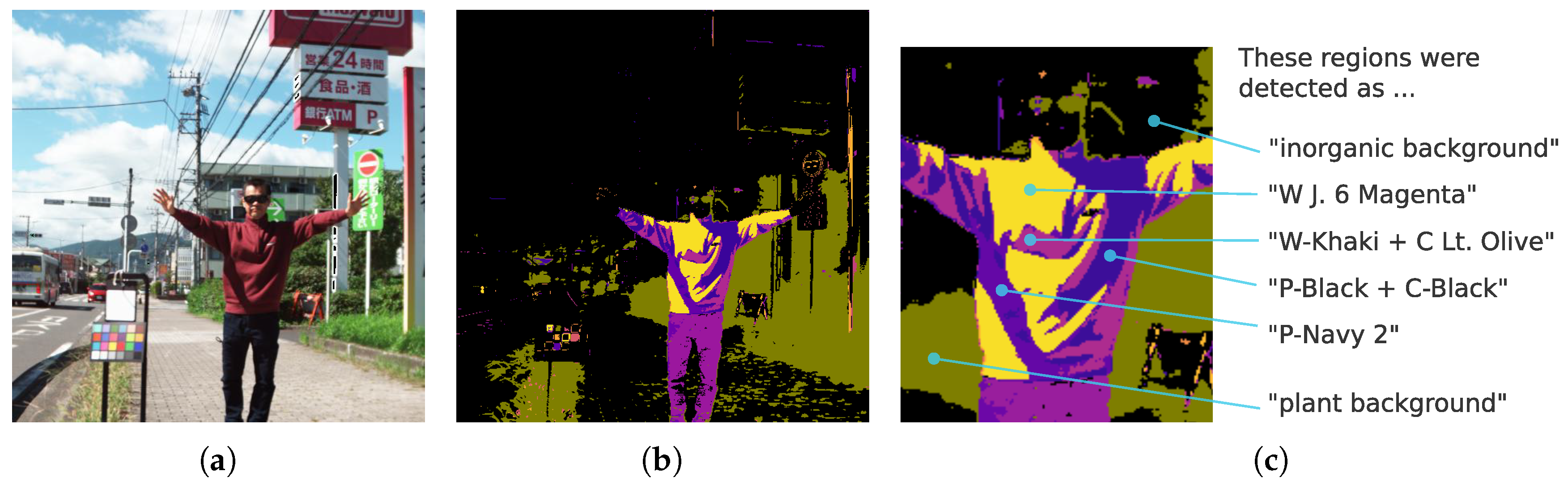
Figure 22.
Samples of detected clothing not included in the training dataset. A single case misidentified as “plant” (red circle). (a) Pseudo-color image. (b) 4-band Optimal Wavelength Set (OWS4-1) MLP predictions.
Figure 22.
Samples of detected clothing not included in the training dataset. A single case misidentified as “plant” (red circle). (a) Pseudo-color image. (b) 4-band Optimal Wavelength Set (OWS4-1) MLP predictions.
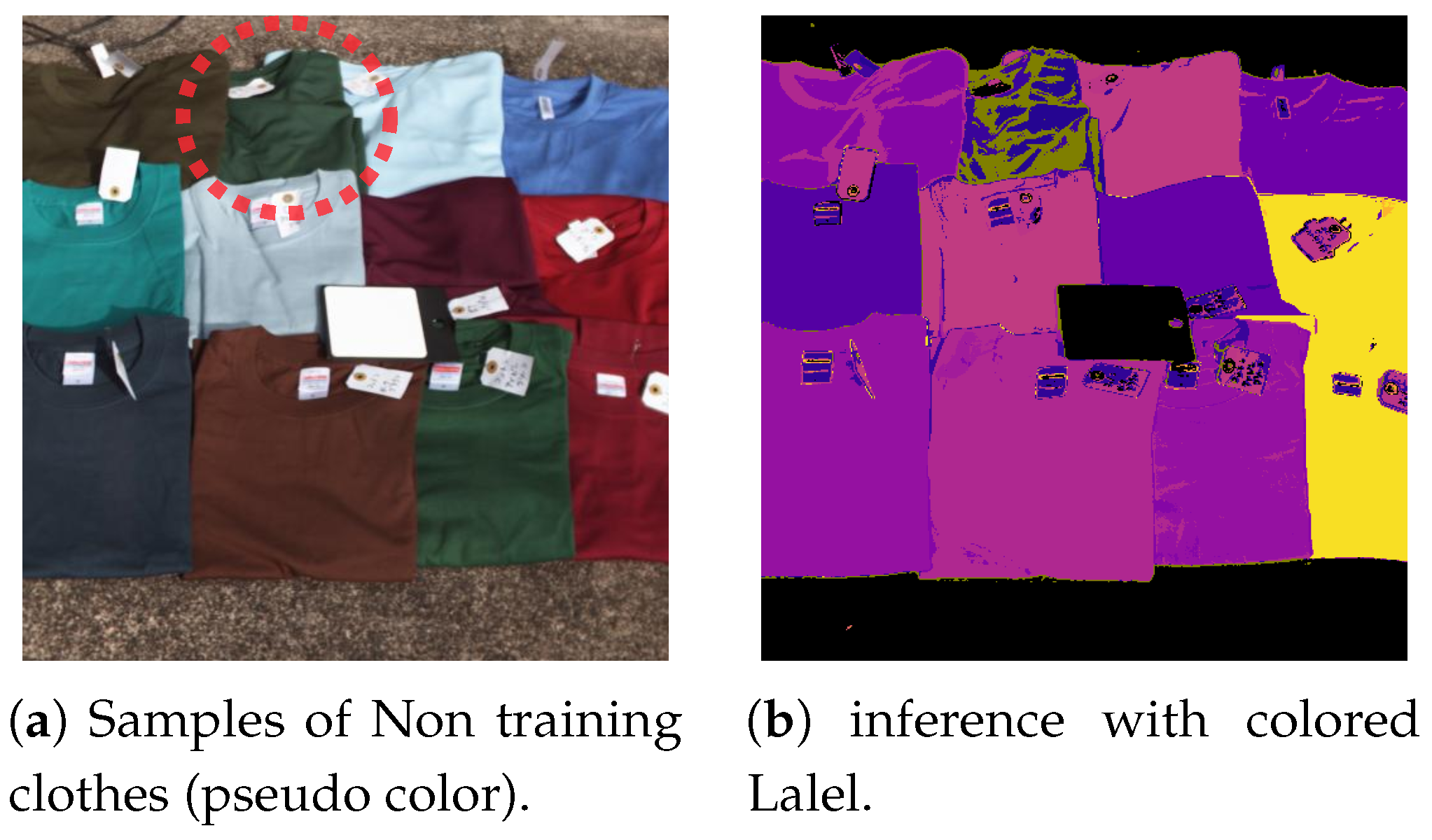
Figure 23.
Example of a street scene containing background objects likely to be misclassified as clothing. (a) Pseudo-color image. (b) Multi-label predictions by the 4-band Optimal Wavelength Set (OWS4-1) MLP.
Figure 23.
Example of a street scene containing background objects likely to be misclassified as clothing. (a) Pseudo-color image. (b) Multi-label predictions by the 4-band Optimal Wavelength Set (OWS4-1) MLP.
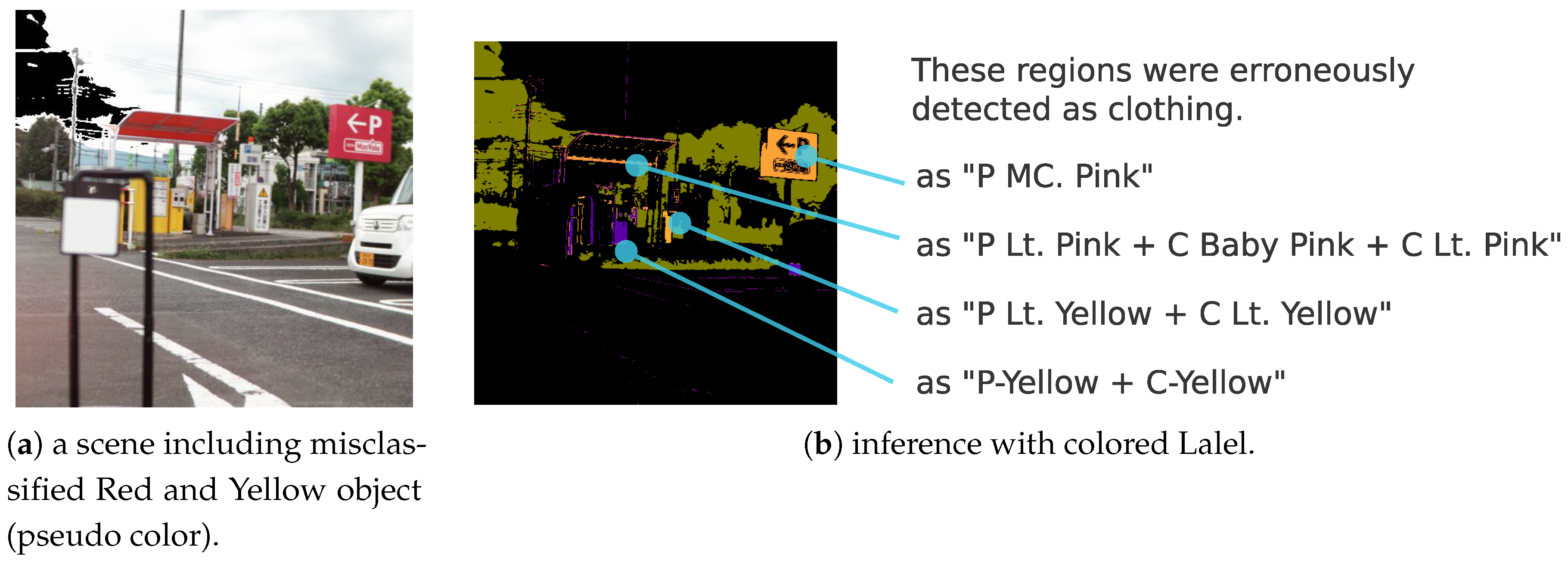
Figure 24.
White (blue circle) or black (red circle) wool garments can be missed. (a) Pseudo-color image. (b) Multi-label predictions by the 4-band Optimal Wavelength Set (OWS4-1) MLP. Gray cotton (green circle) garments can be missed. (c) Pseudo-color image. (d) Multi-label predictions by the 4-band Optimal Wavelength Set (OWS4-1) MLP.
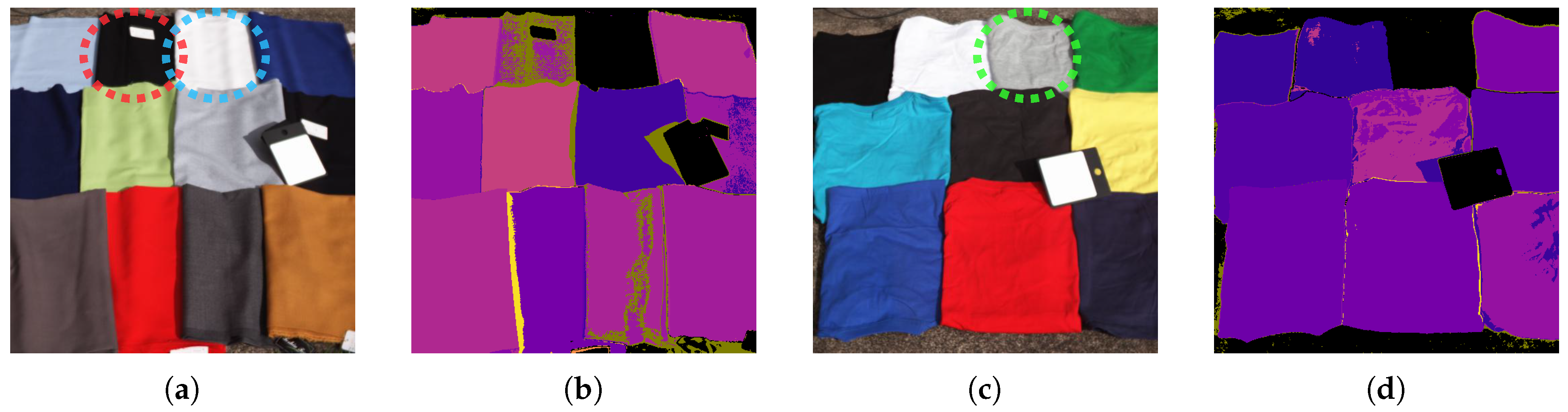
Figure 25.
Examples of clothing materials deviating from this study’s “clothing hypothesis” (genuine leather and synthetic leather). (a) Pseudo-color image (genuine leather). (b) 4-band Optimal Wavelength Set (OWS4-1) MLP inference (genuine leather). (c) Pseudo-color image (synthetic leather). (d) 4-band OWS4-1 MLP inference (synthetic leather).
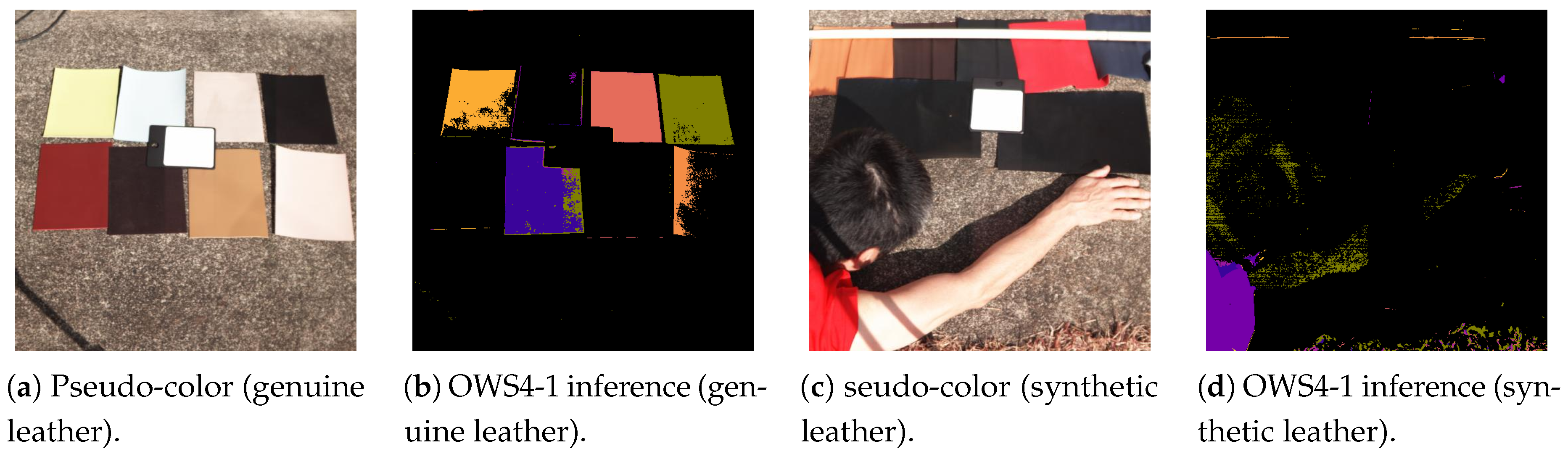
Figure 26.
Overall inference examples from the 4-band Optimal Wavelength Set (OWS4-1) MLP (top: pseudo-color image; bottom: classification result with bright yellow for clothing and black for background). (a) Scenes not included in the training dataset. (b) Scenes used in training.
Figure 26.
Overall inference examples from the 4-band Optimal Wavelength Set (OWS4-1) MLP (top: pseudo-color image; bottom: classification result with bright yellow for clothing and black for background). (a) Scenes not included in the training dataset. (b) Scenes used in training.
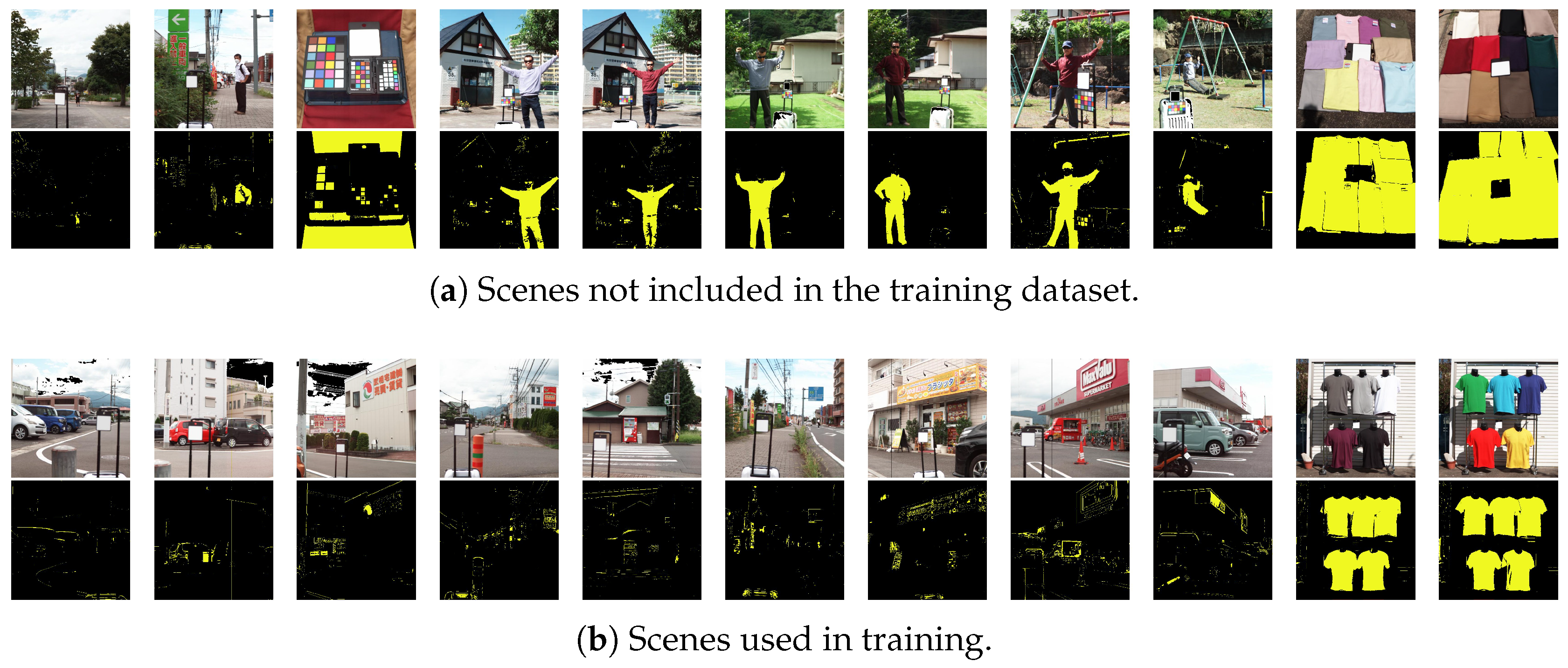
Figure 27.
(a) 4-band reflectance and (b) hyperspectral reflectance for four types of green/blue garments.
Figure 27.
(a) 4-band reflectance and (b) hyperspectral reflectance for four types of green/blue garments.
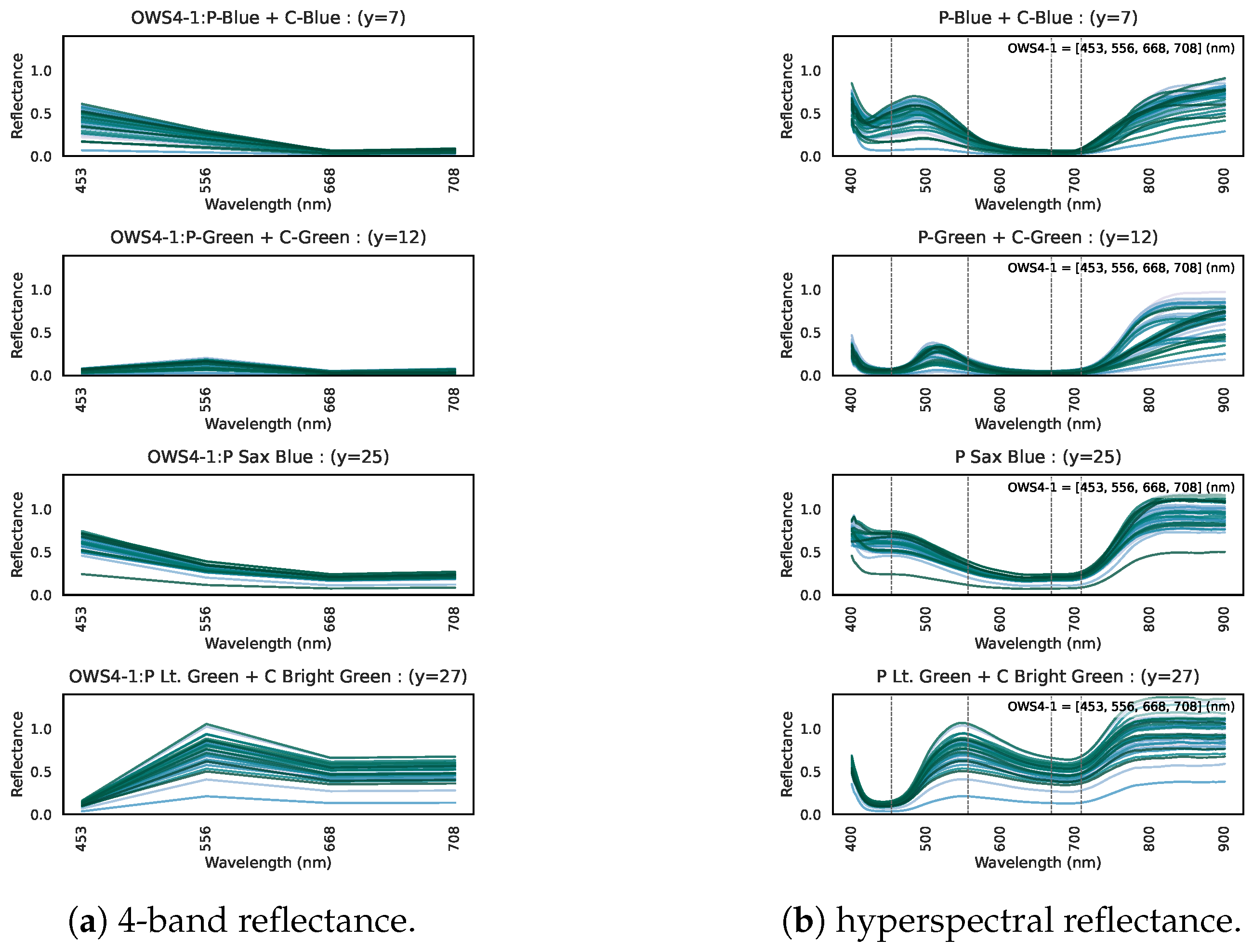
Figure 28.
(a) 4-band and (b) hyperspectral reflectance for plants.
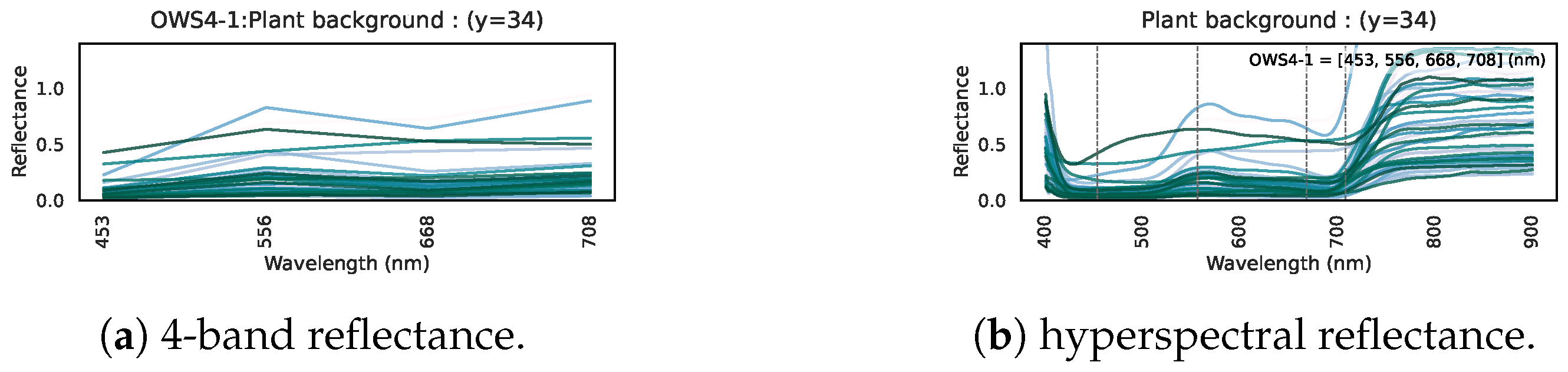
Figure 29.
Reflectance at (a) 4 bands and (b) full hyperspectral data for white garments (polyester, cotton, and wool).
Figure 29.
Reflectance at (a) 4 bands and (b) full hyperspectral data for white garments (polyester, cotton, and wool).
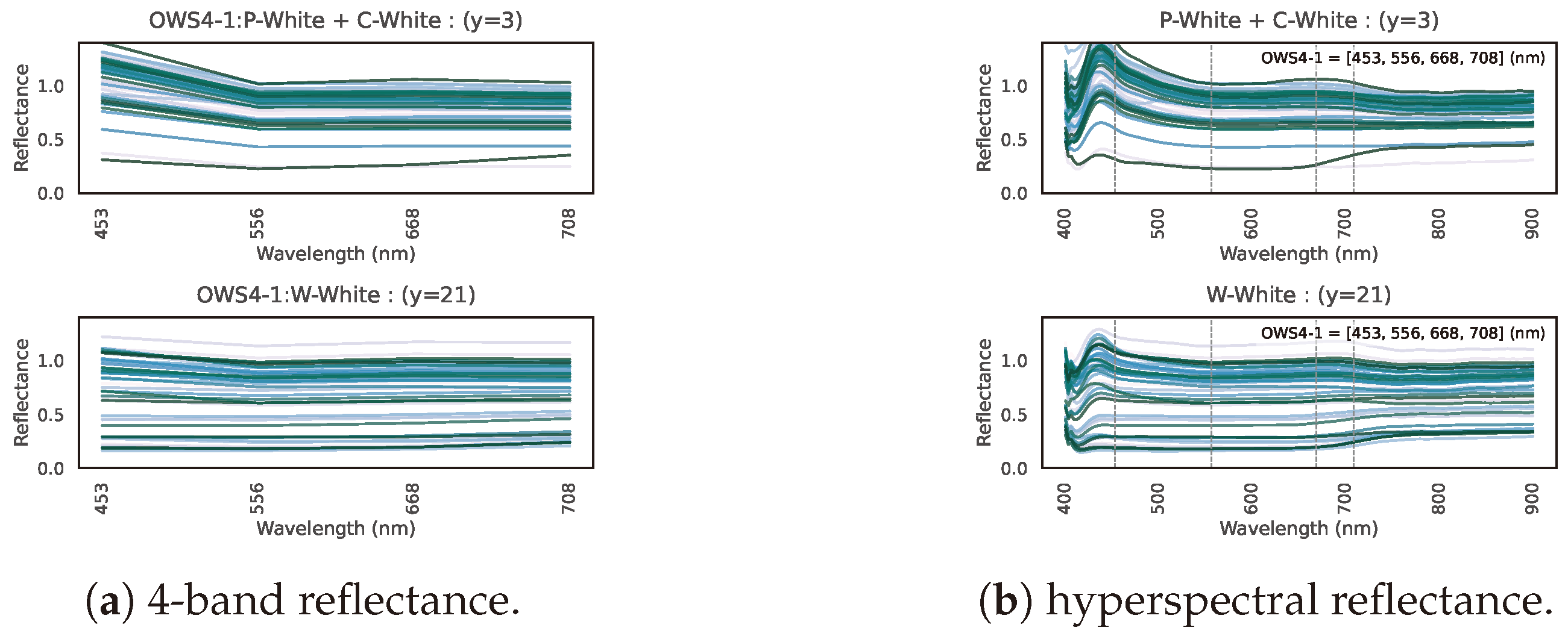

Table 1.
List of 41 labels (label name, index, and R-channel intensity in the labeled image).
 |
1 Polyester is abbreviated as “P-”. Cotton is abbreviated as “C-”. Wool is abbreviated as “W-”. Toray is abbreviated as “T.” Gabardine is abbreviated as “G.” Mixed Color is abbreviated as “MC.” Josette is abbreviated as “J.” Athletic is abbreviated as “A.” Glimmer is abbreviated as “Glim.” Grayish is abbreviated as “G.” Dark is abbreviated as “D.” Light is abbreviated as “Lt.”
Table 2.
Comparison of five machine learning approaches: Radial Basis Function Support Vector Machine (RBF-SVM), Random Forest, Gradient Boosting, Adaptive Boosting, and Multi-Layer Perceptron (MLP).
Table 2.
Comparison of five machine learning approaches: Radial Basis Function Support Vector Machine (RBF-SVM), Random Forest, Gradient Boosting, Adaptive Boosting, and Multi-Layer Perceptron (MLP).
 |
Table 3.
Results of preliminary experiments on the Multi-Layer Perceptron (MLP) hidden units (6/10/16/32/64). Performance plateaued with 16 units × 2 layers.
Table 3.
Results of preliminary experiments on the Multi-Layer Perceptron (MLP) hidden units (6/10/16/32/64). Performance plateaued with 16 units × 2 layers.
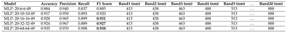 |
Table 4.
Accuracy/Precision/Recall/F-measure for 167-band Multi-Layer Perceptron (MLP-167).
 |
Table 5.
Comparison of evaluation metrics for Multi-Layer Perceptron (MLP) models with reduced dimensions by uniformly subsampling wavelengths or by Principal Component Analysis (PCA).
Table 5.
Comparison of evaluation metrics for Multi-Layer Perceptron (MLP) models with reduced dimensions by uniformly subsampling wavelengths or by Principal Component Analysis (PCA).
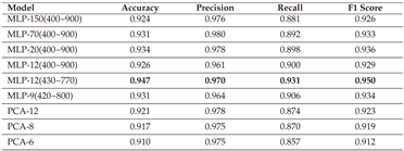 |
Table 6.
Final Optimal Wavelength Set (OWS) combinations and evaluation metrics for 4-, 5-, and 3-band searches.
Table 6.
Final Optimal Wavelength Set (OWS) combinations and evaluation metrics for 4-, 5-, and 3-band searches.
 |
Table 7.
Performance of Additional Wavelength Set Configurations: Agricultural-Use and Range-Limited (Visible-Only and Near-Infrared-Only) Examples.
Table 7.
Performance of Additional Wavelength Set Configurations: Agricultural-Use and Range-Limited (Visible-Only and Near-Infrared-Only) Examples.
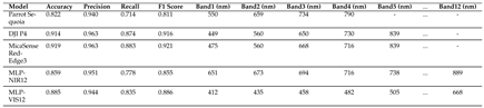 |
Table 8.
Comparison of speed, memory, and detection score for a sample test image.
 |
1 Multi-Layer Perceptron (MLP).
Disclaimer/Publisher’s Note: The statements, opinions and data contained in all publications are solely those of the individual author(s) and contributor(s) and not of MDPI and/or the editor(s). MDPI and/or the editor(s) disclaim responsibility for any injury to people or property resulting from any ideas, methods, instructions or products referred to in the content. |
© 2025 by the authors. Licensee MDPI, Basel, Switzerland. This article is an open access article distributed under the terms and conditions of the Creative Commons Attribution (CC BY) license (http://creativecommons.org/licenses/by/4.0/).
Copyright: This open access article is published under a Creative Commons CC BY 4.0 license, which permit the free download, distribution, and reuse, provided that the author and preprint are cited in any reuse.


