
Submitted:
20 February 2025
Posted:
21 February 2025
You are already at the latest version
Abstract
The article presents the problem of efficiency of the distribution system with different strategies - “Pull” or “Push” and different sizes of distribution networks. The problem relates to the case where products are shipped to the customers through the distribution network. The problem addressed by the author concerns the method of replenishing stocks in these warehouses by the production plant. The author hypothesized that the profitability of using the Pull or Push strategy depends on the number of warehouses - and vice versa: not only how many warehouses (or distribution centers) there are, but also how the stocks stored in them are replenished. For this reason, both of these decision problems should be considered together. The profitability of a particular combination of these two strategies depends on the costs of the logistics and production processes, the parameters of the distributed products and the parameters of demand. This hypothesis has been confirmed. The author developed a simulation model to calculate the effects of applying a given strategy on the availability of these stocks to customers and the levels of stocks. The model was used to simulate different scenarios (different demand distribution - Gauss or Gamma and different demand fluctuations). The results obtained can be further used to calculate the economic efficiency of these strategies, which is also presented in the article as an example of the application of this model. With more expensive goods and higher fluctuations in sales, there is a certain tendency to centralize storage and use Pull strategies. A given strategy - Pull or Push - is not necessarily related to a given competitive strategy (competing with lower costs or better service). Each of these strategies may result in lower total costs or higher level of Logistics Customer Service measured by the availability of the products to customers.
Keywords:
pull strategy
; push strategy
; centralization of stocks
; economical efficiency of distribution strategies
; logistics customer service
1. Introduction
Significant decision-making problems, which link manufacturing and logistics strategies include determining where the final shape of a product is given, where it is stored and from where it is shipped to the customer. These problems are related to the choice between a PULL or PUSH strategy.
Pull and Push strategies can be applied at different stages of logistics and production processes, what is presented in the Figure 1.
Two strategies in the field of production, and also partially in the distribution of final products are “Make To Stock” (MTS) and “Make To Order” (MTO). These strategies have an impact both on the costs (production, logistics) and the level of logistic customer service, so (indirectly) they can affect the level of sales (Figure 2). The choice of a given strategy has impact both on a level of inventories, capacity of production and logistics potential, location of facilities (production plants, warehouses, distribution centers, used technology (mechanical, automated) and as a result on the variable and fixed costs of production and logistics processes (warehousing, inventory management, transport).
As the MTS strategy allows for stabilization of production processes and production costs may be lower due to better use of the production potential or production in longer series. The impact on the level of customer service is not clear. In the MTS system products are already manufactured and can be used for sale, especially if the products are stored close to customers. In the MTO system, products still need to be produced, which means that the order fulfillment time may be longer.
On the other hand, products are produced for which there is currently a demand. This strategy can be used when products are produced according to customer requirements (product type, product parameters – “Non-standard products”). In many cases, it is difficult to compare them. For this reason, the comparison presented in this article was made for a specific problem - how to replenish products (“Standard products”) in the own distribution network before shipping them to the final recipient.
The choice of a distribution strategy has an impact on the levels of stocks in a distribution network. The level of these stocks is also influenced by the degree of centralization of this network (number of warehouses). This raises the question of whether these two decision-making problems should not be considered together. The benefits of “pulling” or “pushing” depend on how many warehouses there are, so the effectiveness of the degree of centralization depend on how the stocks in these warehouses are replenished.
2. Materials and Methods
The aim of the research, the results of which are presented in the article, was to create recommendations for companies regarding the choice of the optimal logistics strategy for distribution (“Pull” or “Push” strategy and the optimal number of warehouses in the field of distribution).
The specific objectives were:
- Demonstrate that there is a need to combine two decision problems
- determining the optimal number of warehouses in the distribution network;
- determine the choice of replenishment strategy for these warehouses (choice between “Pull” and “Push” strategy)
- 2.
- Presentation of how to perform calculations to choose the optimal strategy.
- 3.
- Checking how the size of the distribution network, in combination with a given replenishment system (pull or push) in this network, affects the efficiency of production and logistics processes.
This was demonstrated through simulations conducted by the author using a simulation model he developed. The purpose of developing this model and running simulations using it was to see how the size of a distribution network, combined with a given replenishment system (Pull or Push) in that network, affects the efficiency of production and logistics processes. The model can be used to calculate process parameters alone - the level of the inventories, the availability of products (stocked in warehouses) to customers, the amount of production capacity required. Once the cost elements are taken into account, it can be used to calculate the costs of a given strategy.If this model is expanded to include the costs of logistics processes, it will allow to calculate the economic efficiency of different strategies or combinations of different strategies. The model can be further expanded by adding production and material procurement costs.
The model uses one measure of the level of logistics service, namely the availability of inventory in a distribution warehouse, which affects the “opportunity cost of sales.” The model calculates how many products could not be sold if the inventory level was insufficient. Thus, it measures the percentage of actual sales versus projected sales.
The tool used to build this model was the Excel spreadsheet, which used formulas to generate daily demand based on an assumed average daily demand and standard deviation. Simulations were carried out for different standard deviations of demand and for two types of the demand distribution : Gaussian and Gamma distribution with the us Excel’s function “IF”, in which the “GAUSS.DIST” or “GAMMA.DIST” function appears, respectively. This is because the model replicates (simulates) the operation of the system throughout the year. The idea was not to use average yearly data, but to reproduce the functioning of a real system as precisely as possible. This function allows you to take the standard deviation into account. The demand on each day is generated by a computer based on the specified average daily demand, the Gaussian or gamma distribution and the standard deviation of demand.
The inventory level on a given day is derived from the inventory level on the previous day, the volume of deliveries on that day and the sales on that day.
As for the level of production and the related volume of production potential, in the case of the Pull strategy, the volume of production is adjusted by the current orders of the distribution centers and in Push it is based on the projected needs of these centers. In other words, the model adjusts the production capacity so that warehouse orders can be fulfilled 100%. This means, of course, that if demand is variable, production capacity will be unused at certain times, which justifies extending the model to include production costs. This problem will occur especially in the case of seasonal demand.
3. Results
3.1. Analysis of the Literature
3.1.1. Pull – Push Strategies and Systems
Pull and Push strategies are the basic production and logistics strategies described by some authors as ‘functional’, that is, according to the classical classification, at the lowest level, below competitive strategies, above which are global strategies [1]. At this level, another “functional” strategy is defined - the size of the distribution network (strategy of centralizing or decentralizing the warehouse network). The choice between these different strategies is a decision-making problem that should be solved based on a cost-effectiveness calculation.
Strategies at all levels should be coherent with each other, i.e. the strategy at a lower level should follow from the strategy at a higher level. So, as it seems, the choice of competitiveness strategy (competing either on price or on quality elements) determines the choice of production or logistics strategy. However, even within a given competitiveness strategy, a choice of production and logistics strategies can be made, as they affect both quality elements (level of customer service) and cost elements. The effectiveness of their application is determined by various factors and, in order to assess it, their cost-effectiveness must be calculated.
In the production field, Pull and Push strategies are “Make To Stock” (MTS) and “Make To Order” (MTO) respectively [2,3].
MTS and MTO are two strategies that can be used in different markets, for different customers and products, so it doesn’t always make sense to compare them. The sensitivity of manufacturing strategy alteration towards changing customer requirements is dependent among others on distinct product characteristics [4]. The choice of a particular strategy can be influenced by the characteristics of demand (volume of demand, predictability, volatility), the length of lead times and the nature of cooperation in supply chains [5]. It is recognized in the literature that MTO should be chosen for low-volume products, special products with a wide assortment and low unit volume, manufactured according to individual customer orders and MTS in mass, repetitive production, for high-volume and standard products with a predefined and narrow assortment [2]. In addition to customer demand characteristics, there are also conditions for the successful implementation of these strategies - in the case of MTOs, this condition is a high degree of integration with suppliers of production materials [6]. However, if they can be used as alternative strategies in a given enterprise, the benefits of choosing a given strategy should be compared.
There can be combinations and modifications of MTO and MTS strategies. The strategies that combine their advantages are postponement or Assembly To Order (ATO). In fact managers of manufacturing companies usually employ more than one strategies [7]. These include Engineer–to-order (ETO). “ETO firms” produce complex, “one of a kind products” and desire shorter lead time as a key component to cost competitiveness. Unlike other manufacturing models, such as make–to-stock or make-to-order models, the design for an ETO product is not realized until after the engineering process has been completed. Therefore, the problem becomes the determination of an accurate schedule within a complex transactional process for jobs, which have not even been designed yet [8].
For Engineer and Design-To-Order (ETO and DTO) industrial environments proper tools are need. These are for example Plan For Every Order (PFEO), which collects information on both suppliers and materials, improving both the management of materials and spaces and communication between the company and suppliers [9], tools for real-time performance of processes measurement based on digital visualization (DV), that uses novel technologies to enhance decision-making [10].
In the ‘Push’ strategy, high efficiencies can be achieved in both production and logistics processes, but may create high level of inventories. The choice between Pull and Push systems is not only a choice between the cost of inventory and storage on the one hand and production, transportation or ordering on the other, but the cost of lowered logistics customer service level should also be taken into account.
The choice between one strategy and another affects at least three basic elements of Logistics Customer Service - availability of inventory in the warehouse, delivery time, on-time delivery, which are all interrelated. If inventory is available in the warehouse it can be shipped quickly to the customer. Pull systems are supposed to cope better with the variability of demand processes, but can result in long delivery times if they are not flexible [11]. However, the delivery time depends on the distance over which the goods are shipped and also the timeliness of delivery. These factors are taken into account by some authors, as exemplified by the work of Ni [12], who included the cost of order processing delays in the model he developed. In this article, availability of stocks (AoS) in the warehouse will be used as a measure of Logistics Customer Service.
The problem of uncertainty is related to the choice of an appropriate strategy. These strategies can be reactive (buffering) and proactive (redesign). Angkiriwang et. al. [13] made three suggestions based on four case studies. One of the conclusions interesting from the point of view of the issue discussed here is that to achieve better flexibility, companies focus more on buffering than on proactive strategies. Inventory therefore allows the company to adapt to changing customer needs.
In the Pull strategy, products, even if they have already been ordered, can be stored for some time because they can wait to be loaded and shipped to the customer. In addition, they can be sent from the production plant not directly to the customer, but to a warehouse, or a distribution centre. In such a system, in both strategies, the manufactured products are stored in distribution warehouses, where they await customer orders. However, also in this case, there is a need to choose between the PULL or PUSH strategy in replenishing stocks in these warehouses. Products can be dispatched (‘pushed’) to the distribution network after production (either immediately or after they have accumulated a shippable quantity). They can also be dispatched (‘pulled’) on the basis of orders that warehouses (distribution centres - DC’s) place when stock of a particular product falls to a certain level.
3.1.2. Pull and Push Strategies– Factors of Effectiveness
Push strategy (MTS) may be cheaper if it allows for lower production or transport costs. This strategy can provide a higher level of logistical customer service as measured by the availability of product stock. However, such security may be illusory, as it may be stocks of the wrong products that the customer don’t need at that moment. A very similar problem is associated with the choice of the degree of centralisation of the warehousing network - in a geographically extensive system based on a network of warehouses, which are located close to customers, products are ready to be dispatched or collected by the customer. However - again - these may not be the products the customers want. Such a problem arises when the assortment of products is wide and demand is difficult to predict.
Moreover, it is not obvious that any one strategy is more effective in terms of stock levels. For example, Grosfeld-Nir et. al. [14] conclude that:
„Surprisingly, we find that often push out performs pull, i.e. push systems accumulate less WIP than pull systems, while maintaining higher PT”
Also, a study conducted by Masuchun et. al. [15] confirm that a Push strategy can outperform a Pull strategy in terms of customer service levels and throughput, but a Pull strategy can outperform a Push strategy in terms of total inventory. While the latter conclusion is obvious, as that is why the strategy is used, to avoid costs but also inventory risks, the former may seem surprising. The occurrence of such seemingly paradoxical situations in terms of both the choice between Pull and Push and the degree of centralisation of the storage network is confirmed by case studies that can be found in the literature.
A given strategy does not have to be related to either a competitive strategy or the specifics of a given manufacturing industry, but is an individual choice of a given company, as evidenced by the results of various studies. For example, a study of supply chain strategies used by light vehicle manufacturers in South Africa, showed that manufacturers use both lean and agile supply chain strategies [16] (Ambe 2014).
The problem is, of course, very complex, because the efficiency of production and logistics systems is not a matter of simply choosing between Pull and Push, or a combination of these systems, but of managing them properly. For example - since the execution processes of production processes have a large impact on energy consumption, Tan et al. have developed, among other things a matrix-geometric method of effective Make-To-Order process management to increase energy efficiency [17].
In fact, the Make-To-Order system, if it is to be effective, requires an efficient process management system, including inventory management. Therefore, research is being conducted on this problem an example of which is the Cyber-Physical Logistics System (CPLS) developed by Park et. al. [18].
Above all, however, it requires proper management of processes throughout the supply chain and appropriate cooperation with suppliers. This problem was addressed by Li et. al. [19], who formulated a control model that takes into account the dynamic responses of customers to the joint implementation of these strategies in order to minimize the cost of disruption. This model takes into account the inventories in this system, which is worth emphasizing, also in the context of the considerations carried out in this article, that even if the effect of the Pull system is to reduce the level of inventories, it does not mean their complete elimination.
3.1.3. The economic efficiency of the PULL AND PUSH strategy and optimization models
Pull and Push strategies can be used even in one company to manage specific product groups. Such a view is presented, for example, by D’Alessandro et. al. [20], who give the example of a chemical company that applies to MTS or MTO strategies to specific product groups based on demand volume and variability. However, according to the author of this article, even with standard products, these two strategies can be implemented and are alternatives to each other. And it is for such a case that simulations have been carried out, the results of which are presented in this article.
For optimization in both decision-making and process management in various systems developed various models presented in the literature. For example Schneckenreither et al. [21] presented a flow time estimation procedure for dynamically setting lead times in MTO systems, using an artificial neural network.
The problem of selecting a particular strategy using optimisation models is widely described in the literature, which presents both general-purpose models [22,23,24,25,26] as well as those relating to specific industries such as: paper and pulp industry (Lehtonen 1999) and the food industry (Van Donk, 2001).
The cost aspect is important in any strategy, as are the qualitative aspects. A study carried out by Ciechanska and Szwed [27] to compare the effectiveness of the MTS model and the MTA (Make-To-Availability approach) showed that the MTA model can effectively meet customer requirements. Surprisingly, however, it may seem that the cost of this was the need to keep inventory at relatively high levels. It is also worth noting that the authors used the category of « opportunity cost », which was taken into account by Puchkova et. al. [28] in their model, which considers various options for inventory control strategies. The optimal solution minimizes the total cost objective function (production cost, inventory holding cost and lost demand cost.
The problem of customer service is particularly important in the MTO (Pull) system and it is particularly challenging for make-to-order companies to achieve a high delivery reliability. In order to solve this problem Mundt and Lödding [29] built a simple model-based procedure to determine delivery times using the throughput diagram with early available information. This problem has been addressed by many authors over the years. For example, Park et. al. [30] proposed the delivery date decision support system which integrates the marketing and production planning functions with the consideration of the current capacity and workload smoothing. The system has been implemented in a rotating machinery shop in South Korea.
In MTO strategy the accurate estimation of processing time is very important. To solve this problem tools like Workload control (WLC) are developed [31].
Capacity planning is important for an efficient production planning in make-to-order (MTO) and assemble-to-order (ATO). Filho and Marçola [32] proposed a linear programming model to plan the operations using Annualized hours (AH). This model has been implemented in a company that produces agricultural implements.
A management system that takes into account possible disruptions in the production system may also be necessary. To solve this problem, Wang et. al. (2024) [33] proposed a prediction method based on spatial and temporal (ST) characteristics of the production process.
The problem of the risk of reduced quality of service in an MTO strategy is highlighted by, for example Prasetyaningsih et al. [26], who have developed a model to calculate the profitability of this strategy for the case of a company that orders raw material after receiving orders from customers. The lead time is very long, making it impossible for the company to fulfil the customer’s order in time and have to give a discount of 25 - 30% of the value of all purchases.
Models have also been developed that take into account the complexity of supply chains or networks. For example Hammami et. al. (2022) [34] have developed a model of a two-stage decentralised supply chain works for customised production in a stochastic environment. The model was developed to find the optimal strategy taking into account the relationship between local delivery times, total delivery times, prices, demand and profits, and the impact of firms’ production capacity.
Fisher [35] have developed a model distinguishing between functional and innovative products and between physically efficient and market-responsive supply chains. Products characterised by, among other things, a constant (predictable) demand pattern and long product life cycles require cost minimisation and high resource utilisation, while innovative products characterised by demand variability and short life cycles should respond to the market with a supply chain that has additional capacity and is more flexible. This model has been empirically tested and has found some validation [36].
There is an abundant literature concerning the problems of managing and optimizing hybrid systems combining Pull (Make-To-Order) and Push (Make-To-Stock) - strategies and models, [37]. And also models have been developed for evaluating hybrid versions of MTO AND MTS strategies in specific cases and specific sectors of the economy. For example, Elmehanny et al. developed just such a model for production planning in garment industry [38]. Specific problems are related to the size of the company and therefore Perona et al. [39] developed a model to support inventory management decisions in a MTO–MTS context implementation in small and medium sized enterprises (SMEs).
Combining strategies raises new decision-making problems and the need to develop new tools and methods for solving decision-making problems and calculating the profitability of the solutions used. In case of combined MTS and MTO strategies in order to optimally positioning inventories strategic as well as tactical decoupling points should be identified [40].
To optimize a hybrid “Make-to-Stock-Make-to-Order” environment, Khakdaman et. al. [41] developed a novel optimization model for medium-term production scheduling that incorporates three types of uncertainty: suppliers, processes and customers, using Lp-Metric methodology and IBM ILOG CPLEX optimization software.
Tsubone and Kobyashi developed the production seat booking system with a combination of make-to-order and make-to-stock in production environment [42]. They formulated a production planning model in order to measure the influence on the manufactuiring performance, the buffer inventory, the degree of the delivery date satisfaction.
MTO strategy is characteristic for Lean Management concept and Just-In-Time strategy. For Lean organizations the ‘Mapping Tool for Make-To-Order companies’ (2MTO) was developed, to analyse and achieve Lean benefits in high-variety-low-volume job shops. 2MTO was explained making reference to an Italian precision mechanic company [43].
Some of the works cited above deal with the very important problem of increasing the efficiency of the systems by proper management. The problem discussed in this article, on the other hand, concerns the issue of optimization and selection of a given strategy under unchanged and comparable conditions of using Pull or Push system.
The literature also contains interesting case studies of companies that have implemented these strategies. Here are some examples.
A company of plastic packaging segment classified products according to the ABC analysis of the production and used the mixed pull system, where items in categories A and B should be on supermarket (Push - MTS) and products and items in category C should be made according to their requests (Pull - MTO) [44]. It is worth noting that this resulted not only in a change of distribution strategy, but also necessitated a reorganization of production processes at the factory.
The need to combine these strategies and use combinations of them for different products postulated by the authors cited above is also supported by case studies from other industries - such as agricultural equipment manufacturing (Köber, Heinecke 2012) [45].
When implementing Pull, there is a need to increase the efficiency of this system so that deliveries to customers can be made efficiently. However, the use of such a strategy can be enabled by the fact that customers are willing to wait for their product. An example of such a strategy is Dell, which was the first company to introduce a configure-to-order (CTO) model in which customers can customize computers according to their requirements. The company introduces new products and technologies faster than its competitors. However, shipping times have lengthened (about 7-14 days) because computers are produced after an order is placed [46].
This brings up an aspect that is probably not often mentioned in publications - namely, the logistics aspect. For even if a company actually manages to increase the flexibility of its production system - there remains the question of shipping these goods to customers. In the PUSH system, the products are already produced, they can be loaded, combined with other products to make the best use of the cargo space of the means of transport. In the PULL/MTO system, such possibilities are already limited. Moreover, in the context of the ever-increasing interest in ecology, it seems that MTS/PUSH should be the preferred strategy. Similar problems as in the production field also occur at a later stage, i.e. the physical distribution of goods.
3.2. Effectiveness of Pull and Push Strategies in the Production – Distribution
3.2.1. The model and Its Assumptions
The model is a modification of models already developed to evaluate the efficiency and economic effectiveness of the degree of centralization of the warehouse network in the distribution field (Milewski, 2020 [47]; Milewski, Wiśniewski 2022 [48]). The model is applicable to situations where standard products are produced, and the decision problem is whether to “Push” products after production, or whether warehouses order products based on their needs (“Pull”). So one could say that warehouses are “customers” for the production. The model presented in this article is a modification of those models because it takes into account not only the number of warehouses but also how stocks are replenished in those warehouses.
The following sections presents the results of a simulation conducted by the author of the article using a simulation model to compare the effectiveness of Pull and Push strategies in the field of distributing goods to customers.
The first step was to present the results of a simulation of the impact of the distribution strategy on inventory levels and availability (3.2.2.).
Subsequently, it was shown how the results of these simulations can be used to calculate the economic efficiency of these strategies (3.2.2.).
The simulations were carried out for two demand distributions: Gaussian and Gamma, and for each of these distributions, different deviations of demand from average demand.
3.2.2. Impact on Logistics-Production Potential
The first parameter and effect of using these strategies was the level of stock availability in warehouses, which can be a measure of logistical customer service. The simulation results are presented in Table 1 and Figure 3 and Figure 4.
CD’s are replenished in 3 ways:
- “Pull daily” in quantities to meet actual demand;
- “Push daily” also in small but fixed amounts according to forecasts of demand;
- “Push weekly” in fixed amounts corresponding to the average weekly demand.
This third option applies when e.g. rail transport is used, which is less flexible than road transport, and deliveries are made on schedule.
In the first step, simulations were carried out for a Gaussian distribution and standard deviations of 5% and 30% from the average demand.
For small fluctuations in sales (5% of Standard deviation of average sales) deliveries in large quantities (“Push weekly”) are the most effective in this regard. A high level of customer service is also ensured by “pushing” goods daily from the plant to the warehouses. As the number of warehouses increases, the level of customer service drops very sharply in weekly deliveries, while in the “Push daily” remain high.
Daily “pulled” deliveries result in a lower level of customer service. Only with 6 distribution centers they offer a higher level of service than weekly “Push” deliveries. However, in most cases, the best customer service is associated with “Pushing” deliveries in small quantities (daily).
The situation changes when demand is more volatile (standard deviation of 30% of average demand) - in all strategies and variants, the level of customer service measured by inventory availability is lower, but to varying degrees.
Regardless of the number of CD’s in the distribution network, the best inventory availability is again observed for daily “Push” deliveries (Figure 4). This time yet a slightly lower, but also high level of service is observed for daily “Pull” deliveries. In the case of weekly “Push” deliveries, the level of service is much lower. The results of these simulations are not surprising - as expected with greater fluctuations of demand and therefore less predictability of demand, a more flexible system that adjusts the volume of deliveries to actual rather than forecast demand is more efficient from a customer service perspective.
The differences between the levels of logistics service appear to be small. But first, they are due to the probability distributions assumed in the simulations and the data generated by the model developed by the author. Since lower levels of service are observed in practice, there is a need to investigate what the actual probability distributions and sales fluctuations of companies are. The model does not take into account one more service level factor - on-time delivery. This is because it assumes that deliveries arrive on time. Taking into account the delays in deliveries to warehouses would result in either lower service levels or increased inventories.
However, even without considering the above factors, even a small change in the level of logistical customer service can have a big impact on the efficiency of the system. As demonstrated later in the article, deterioration of service by even a few percent can result in high costs of lost sales. Increasing that service by just a few percent as well can also result in a significant increase in costs - for example, inventory maintenance and warehousing.
Table 2 and Figure 5 and Figure 6 presents results of the simulation of the impact of different strategies at the level of stocks for the levels of service from Table 1.
It is, of course, no surprise that inventory levels increase if there is a shift from a “Pull daily” strategy, which is the most flexible, to a “Push daily” strategy. The largest is in “Push weekly” due to larger sizes of deliveries to warehouses. In all strategies, inventories increase if sales fluctuations increase from 5% to 30%. In all strategies, too, inventory levels increase as the number of warehouses increases, which confirms (and explains) the existence of the benefits of the strategy of “centralization of stocks” - better customer service can be achieved with less inventory.
To ensure comparability - calculations were made also for the situation when the level of service in all variants is 100%, what is presented in Table 3 and Figure 7 and Figure 8.
In all variants there were large increases in stocks - even in the first variant - “Pull daily”/1 DC/5% standard deviation. This confirms the relationship known from the logistics literature between service level, sales and costs, that when the service level is already very high, increasing it even by a small percentage requires a large increase in costs.
The differences are larger in the case of “Pull daily” but smaller in the case of “Push weekly, ” which can be explained by the fact that deliveries in larger quantities already result in high inventory levels. The differences increase as the number of warehouses increases, once again showing the benefits of centralizing warehousing and confirming the need to combine these two decision problems. In all variants, increasing the number of warehoues results in a very high increase in inventory levels. This increase is even greater if sales fluctuations are greater.
The purpose of the next simulation was to examine how these strategies affect the amount of production capacity required in the case that customer demand is to be satisfied in 100%. The impact here is weaker than in the case of inventory (Table 4). However, given that the cost of maintaining production potential may be greater than maintaining inventory, there is a need to take this relationship into account as well.
One can see a regularity - the highest required production potential occurs in the “Pull - daily” strategy, and the lowest when products are “pushed out” in weekly volumes. This also seems easy to interpret - “Pull” requires either a flexible production system or a high potential for the system to adapt to changing needs. Schedule deliveries, on the other hand, promote production stability.
If demand has a Gamma distribution, service levels are slightly lower than in the case of Gauss distribution (Table 5 and Figure 9 and Figure 10). The difference, however, is which strategy is more efficient. In the case of Gamma, in almost all cases the level of service is better with daily deliveries than with weekly deliveries. In the strategy “Push Weekly ”, the level of service is slightly better with a single warehouse. However, it decreases to a large extent with more warehouses. Thus, with weekly deliveries to 1 warehouse and a standard deviation of 3%, the inventory availability level was 99.0%. When deliveries were made to 6 DC’s the service level dropped to 97.8%. The situation was similar when the standard deviation was 6%.
Service levels for both Pull and Push daily deliveries also decrease as the number of warehouses increases, but to a much lesser extent than for weekly deliveries.
However, despite not much difference in service levels, the impact of these strategies on stocks is greater. In all cases, stock levels are significantly higher for Gamma than Gauss distributions (Table 6) and in most cases, these differences increase with the number of warehouses. For example, with small standard deviations of demand and 1 warehouse, the inventory level is 126.85% higher in the case of a Gamma distribution than in the case of a Gaussian distribution. If the goods are distributed over a network of 6 warehouses, this difference is even greater, at 155.27%. Stocks in the other variants are also significantly higher than under the Gamma distribution. Interestingly, however, these differences would also be very large if customer orders were fully (100%) satisfied. However, in the case of “Pull daily”, inventory levels are very similar (Table 7). This leads to the conclusion that the quick response strategy allows for a high level of customer service without building up high inventory levels.
The effect of distribution strategy on production potential for Gamma distribution was also analyzed. The results are similar - first, for each strategy, the amount of required potential is the same for each size of distribution network (number of DC’s). Second, the largest production potential is required with the Pull strategy. Thirdly, it is larger with larger sales fluctuations (Table 8). However, in the case of a Gamma distribution - it is more than 30% larger than in the case of a Gaussian distribution.
The simulation results prove that decisions on the choice of replenishment strategy and the size of the warehouse network should be considered together. However, this is obviously not enough to assess the economic effectiveness of a given strategy, as the impact on costs and sales would have to be taken into account.
3.2.3. Economic efficiency of Pull and Push systems
Based on the results obtained from the above simulations, calculations of the economic efficiency of each strategy can be conducted.
The assumptions (data) are shown in Table 9. When calculating the costs, the author of the article tried to make the best use of data on processes and the costs of these processes that occur in economic practice - e.g. in Poland.
The calculation results for the Gaussian distribution are shown in Table 10, Table 11 and Table 12 . They take into account the parameters of shipments and the value of goods and the resulting costs of transportation, inventory maintenance and storage, and the cost of lost sales. Differences in total costs depend on the delivery strategy used but also on the type of product, because size and tonnage impact costs of warehousing and transportation.
The criterion for evaluating the effectiveness of the system is the “Total Cost, ” which includes the costs of inventory and storage, transportation and the costs of “lost sales”.
The costs of lost sales are derived from the level of inventory availability from previous simulations (Table 1). Thus, if the logistical customer service measured by such a parameter is 98.96% for the “Pull daily”/1 DC variant. i.e. the company loses 1.04%. The costs of lost sales are calculating in following way for “Food”:
No of items x Price of a commodity x 1.04%=
32000000 [pcs./year] x 1 [EUR/item] x.04%= 332 EUR/year
which is 11.23% of the “Total Cost” (Table 10).
For this group of products, the share of these costs increases with the number of warehouses in the distribution network and is obviously higher with larger sales fluctuations. As expected, these costs will be higher for more expensive products (Table 12). Which provides justification for including them in cost calculations.
For “Food” (the cheapest) and 5% standard deviation, the lowest Total Costs occurs with regular (“Push every week”) deliveries to 6 warehouses by rail transport. If sales fluctuations were higher (30%) then deliveries to 6 warehouses would also be the most efficient, but with the more flexible “Pull daily” delivery system.
Since the value of the goods and the parameters of the shipments are important factors of costs, it can be expected that for more expensive goods (“Electronics”), deliveries with a higher degree of flexibility will be most effective. And this is indeed the case: with small fluctuations in sales (5%), a system of 6 warehouses is also optimal, yet not the cheapest rail transport every week should be used, but by daily deliveries with road transport, although still in the “Push” system. With larger fluctuations in sales (30%) a centralized system is more profitable. This is also the case of “Clothing”.
For similar delivery parameters in the case of Gamma distribution, costs are higher because there is a higher level of inventory and cost of lost sales are higher. For the first variant - deliveries to 1 warehouse every day in the “Pull” total costs increase as the value of goods supplied increases.
Since, as the cases of companies that have centralized their distribution systems show, centralization is effective in the case of large fluctuations in sales, this strategy should be more favorable precisely in the distribution of Gamma demand and more expensive goods. And so it is: only in the case of cheap “Food” is the network of 6 warehouses still the cheapest.
The simulation results presented here prove the truth of the thesis that these two decision problems - the choice of distribution strategy - Pull or Push, and the choice of the degree of centralization of the distribution network are not two separate decision problems, but should be considered together.
A very important conclusion is that the choice of the optimal strategy has a significant impact on the financial results of companies. In all product cases, in all demand variants and replenishment strategies, the share of the costs calculated here represents a few percent of the revenue value. As expected, the lowest share was found for the cheapest goods (“Food”), and the highest share for the most expensive goods. In all cases, the share increased with the fluctuation of demand. For example: in the case of “Food”, the share of these costs for 1 warehouse supplied with the “Pull daily” strategy and a standard deviation of demand of 5% is 9.23%. If the distribution network is expanded to 6 warehouses, this share drops to 5.72%. However, if demand fluctuations are greater (30%), the share of these costs increases to 11.59%, i.e. with greater fluctuations, the strategy of centralizing storage is more profitable. In the case of more expensive “Electronics”, the share of these costs in the sales value is lower: 2-6%. This may not seem like much, but it is important to remember that many companies only have a few percent profitability. Choosing the optimal strategy is therefore crucial for profitability.
For example, the profitability of the largest Polish companies listed on the Warsaw Stock Exchange is: GRENEVIA (“Elektromaszynowy”) 13% 2023, but in 2020 only 3%. In WIELTON from the same industry, it was only 2 and 3%. In the clothing industry, the profitability of the tycoons of the Polish clothing industry in 2023 will only reach: LPP 9% and VISTULA RETAIL GROUP 8%.
The share of these costs is even higher in the case of a Gamma distribution, especially with 6 warehouses. The share of these costs in the sales value of cheap “Food” is 15.28% for 3% deviations from the average sales, and when sales fluctuate more (6%), this share increases to 19.87%. Even for the most expensive goods (“Electronics”), these costs account for 5.48% and 7.17% of the sales value, respectively.
4. Discussion and Conclusions
The above calculation are examples of calculations that could be made. They are based on the assumptions made regarding primarily storage and transportation costs. For example, it was assumed that the rates for transportation services by rail are 40% lower than by road. However, they may explain why centralization of distribution systems is quite common strategy but also why rail transportation has small share in the transportation market.
The results of calculations support the hypothesis that the choice of distribution strategy - Pull or Push - and the choice of the degree of centralization of the distribution network should be considered together. With more expensive goods and higher sales fluctuations, there is tendency to centralize warehousing and use “Pull” strategies.
This confirms the view, that the important factor of a choice between Pull strategy is the level of production and sales [2] - in the case of low levels and small delivery quantities MTO production and deliveries directly to customer appear to be the optimal solution.
The model assumes that the company loses revenue in proportion to the availability of products in the warehouse. The impact, however, can be broader - the customer may abandon cooperation with the supplier entirely. Logistical customer service can also be measured by other parameters - speed and timeliness of deliveries to customers. The effects of deterioration of these parameters are even more difficult to estimate.
It is difficult to determine the relationship between the availability of stock and the level of customer service and sales. A company that wants to use this model should take into account its individual circumstances and possible customer reactions. Most likely, the level of logistical customer service will be based on customer requirements and this level will be the benchmark. The strategy chosen will be the one that allows the customer to be served at the assumed level and will be the cheapest.
Simulation results also showed that each of these strategies - Pull or Push may be cheaper or result in better customer service, so it is necessary to calculate their economical efficiency using, for example, a model such as the one presented in this article. It cannot be said that a given logistics or production strategy results from a given competitive strategy of the company (low costs or good customer service).
The model does not take into account one more factor - the timeliness of deliveries when warehouses are supplied by the manufacturing plant. This is because it assumes that deliveries arrive on time. Accounting for delays in deliveries to warehouses would result in either lower service levels or increased inventories.
In addition, perhaps one should consider the impact of choosing a particular strategy not only on distribution costs but also on production costs and material procurement costs. Applying a pull strategy and maintaining a high level of logistical customer service requires an efficient production and material procurement system.
The model presented in the article uses hypothetical data generated by a computer program. Once the actual data is entered, it can be used to calculate the effectiveness of a given strategy in a given company.
Any company that wants to use this model would have to use its own demand data, which can differ from company to company, not least because the demand for a product can have its own characteristics. Products are sold and distributed to intermediaries who also have their own purchasing strategy, which will have a significant impact on the characteristics and predictability of demand.
References
- Penc, J. Strategiczny system zarządzania. Holistyczne myślenie o przyszłości; Formułowania misji i strategii: Placet, Warszawa, 2001. [Google Scholar]
- Youssef, K.H.; Van Delft, C.; Dallery, Y. Efficient Scheduling Rules in a Combined Make-to-Stock and Make-to-Order Manufacturing System. Ann. Oper. Res. 2004, 126, 103–134. [Google Scholar] [CrossRef]
- Perera, H.N.; Fahimnia, B.; Tokar, T. Inventory and ordering decisions: A systematic review on research driven through behavioral experiments. Int. J. Oper. Prod. Manag. 2020, 40, 997–1039. [Google Scholar] [CrossRef]
- Hofmann, E.; Knébel, S. Alignment of manufacturing strategies to customer requirements using analytical hierarchy process. Prod. Manuf. Res. 2013, 1, 19–43. [Google Scholar] [CrossRef]
- Chaudhry, H.; Hodge, G. Postponement and supply chain structure: Cases from the textile and apparel industry. J. Fash. Mark. Manag. Int. J. 2012, 16, 64–80. [Google Scholar] [CrossRef]
- Prajogo, D.; Olhager, J. Supply chain integration and performance: The effects of long-term relationships, information technology and sharing, and logistics integration. Int. J. Prod. Econ. 2011, 135, 514–522. [Google Scholar] [CrossRef]
- Tiedemann, F. Demand-driven supply chain operations management strategies - a literature review and conceptual model. Prod. Manuf. Res. 2021, 8, 427–485. [Google Scholar] [CrossRef]
- Grabenstetter, D.H.; Usher, J.M. Sequencing jobs in an engineer-to-order engineering environment. Prod. Manuf. Res. 2015, 3, 201–217. [Google Scholar] [CrossRef]
- Braglia, M.; Di Paco, F.; Frosolini, M.; Marrazzini, L. A new lean tool to enhance internal logistics in Engineer and Design-to-Order industrial environment: Plan for every order. Prod. Manuf. Res. 2024, 12. [Google Scholar] [CrossRef]
- Holopainen, M.; Saunila, M.; Ukko, J. Enhancing the order-to-delivery process with real-time performance measurement based on digital visualization. Prod. Manuf. Res. 2023, 11. [Google Scholar] [CrossRef]
- Liu, L.; Xu, H.; Zhu, S.X. Push verse pull: Inventory-leadtime tradeoff for managing system variability. Eur. J. Oper. Res. 2020, 287, 119–132. [Google Scholar] [CrossRef]
- Ni, G. Replenishment policy for a purchase-to-order seller: A tradeoff between ordering cost and delay cost. Int. J. Prod. Res. 2019, 58, 1239–1254. [Google Scholar] [CrossRef]
- Angkiriwang, R.; Pujawan, I.N.; Santosa, B. Managing uncertainty through supply chain flexibility: Reactive vs. proactive approaches. Prod. Manuf. Res. 2014, 2, 50–70. [Google Scholar] [CrossRef]
- Grosfeld-Nir, A.; Magazine, M.; Vanberkel, A. Push and pull strategies for controlling multistage production systems. Int. J. Prod. Res. 2000, 38, 2361–2375. [Google Scholar] [CrossRef]
- Masuchun, W. Davis, S. Patterson, J. W. Comparison of push and pull control strategies for supply network management in a make-to-stock environment. Int. J. Prod. Res. 2007, 10, 4401–4419. [Google Scholar]
- Ambe, I.M. Differentiating supply chain strategies: The case of light vehicle manufacturers in South Africa. Probl. Perspect. Manag. 2014, 12, 415–426. [Google Scholar]
- Tan, B.; Karabağ, O.; Khayyati, S. Energy-efficient production control of a make-to-stock system with buffer- and time-based policies. Int. J. Prod. Res. 2023, 62, 5809–5827. [Google Scholar] [CrossRef]
- Park, K.T.; Son, Y.H.; Noh, S.D. The architectural framework of a cyber physical logistics system for digital-twin-based supply chain control. Int. J. Prod. Res. 2020, 59, 5721–5742. [Google Scholar] [CrossRef]
- Li, S.; He, Y.; Minner, S. Dynamic compensation and contingent sourcing strategies for supply disruption. Int. J. Prod. Res. 2020, 59, 1511–1533. [Google Scholar] [CrossRef]
- Alessandro, A.J.D.; Baveja, A. Divide and Conquer: Rohm and Haas' Response to a Changing Specialty Chemicals Market. Interfaces 2000, 30, 1–16. [Google Scholar] [CrossRef]
- Schneckenreither, M.; Haeussler, S.; Gerhold, C. Order release planning with predictive lead times: A machine learning approach. Int. J. Prod. Res. 2020, 59, 3285–3303. [Google Scholar] [CrossRef]
- Olhager, J.; Östlund, B. An integrated push-pull manufacturing strategy. Eur. J. Oper. Res. 1990, 45, 135–142. [Google Scholar] [CrossRef]
- Olhager, J. Strategic positioning of the order penetration point. Int. J. Prod. Econ. 2003, 85, 319–329. [Google Scholar] [CrossRef]
- Olhager, J.; Wikner, J. Production planning and control tools. Prod. Plan. Control. 2000, 11, 210–222. [Google Scholar] [CrossRef]
- Olhager, J. The role of the customer order decoupling point in production and supply chain management. Comput. Ind. 2010, 61, 863–868. [Google Scholar] [CrossRef]
- Prasetyaningsih, E.; Ardianto, C.D.; Muhammad, C.R. Reducing customers’ lead time using Make to Stock and Make to Order approach. IOP Conf. Series: Mater. Sci. Eng. 2020, 830. [Google Scholar] [CrossRef]
- Ciechańska, O.; Szwed, C. Characteristics and study of make-to-stock and make-to-availability production strategy using simulation modelling. Manag. Prod. Eng. Rev. 2020, 11, 68–80. [Google Scholar]
- Puchkova, A.; Le Romancer, J.; McFarlane, D. Balancing Push and Pull Strategies within the Production System. IFAC-PapersOnLine 2016, 49, 66–71. [Google Scholar] [CrossRef]
- Mundt, C.; Lödding, H. Coping with the uncertainties of make-to-order production: A new approach for determining reliable delivery times with the throughput diagram. Prod. Plan. Control. 2024, 1–27. [Google Scholar] [CrossRef]
- Park, C.; Song, J.; Kim, J.-G.; Kim, I. Delivery date decision support system for the large scale make-to-order manufacturing companies: A Korean electric motor company case. Prod. Plan. Control. 1999, 10, 585–597. [Google Scholar] [CrossRef]
- Kundu, K.; Rossini, M.; Portioli-Staudacher, A. Analysing the impact of uncertainty reduction on WLC methods in MTO flow shops. Prod. Manuf. Res. 2017, 6, 328–344. [Google Scholar] [CrossRef]
- Filho, E.V.G.; Marçola, J.A. Annualized hours as a capacity planning tool in make-to-order or assemble-to-order environment: An agricultural implements company case. Prod. Plan. Control. 2001, 12, 388–398. [Google Scholar] [CrossRef]
- Wang, S.; Guo, Y.; Huang, S.; Liu, D.; Tang, P.; Zhang, L. A spatial-temporal feature fusion network for order remaining completion time prediction in discrete manufacturing workshop. Int. J. Prod. Res. 2023, 62, 3638–3653. [Google Scholar] [CrossRef]
- Hammami, R.; Frein, Y.; Nouira, I.; Albana, A.-S. On the interplay between local lead times, overall lead time, prices, and profits in decentralized supply chains. Int. J. Prod. Econ. 2022, 243. [Google Scholar] [CrossRef]
- Fisher, M. What is the right supply chain for your product? Harv. Bus. Rev. 1997, 75, 105–116. [Google Scholar]
- Selldin, E.; Olhager, J. Linking products with supply chains: Testing Fisher's model. Supply Chain Manag. Int. J. 2007, 12, 42–51. [Google Scholar] [CrossRef]
- Peeters, K.; van Ooijen, H. Hybrid make-to-stock and make-to-order systems: A taxonomic review. Int. J. Prod. Res. 2020, 58, 4659–4688. [Google Scholar] [CrossRef]
- Elmehanny, A.M.; Abdelmaguid, T.F.; Eltawil, A.B. Optimizing Production and Inventory Decisions for Mixed Make-to-order/Make-to-stock Ready-made Garment Industry. 2018 IEEE International Conference on Industrial Engineering and Engineering Management (IEEM); pp. 1913–1917.
- Perona, M.; Saccani, N.; Zanoni, S. Combining make-to-order and make-to-stock inventory policies: An empirical application to a manufacturing SME. Prod. Plan. Control. 2009, 20, 559–575. [Google Scholar] [CrossRef]
- Wikner, J.; Johansson, E. Inventory classification based on decoupling points. Prod. Manuf. Res. 2015, 3, 218–235. [Google Scholar] [CrossRef]
- Khakdaman, M.; Wong, K.Y.; Zohoori, B.; Tiwari, M.K.; Merkert, R. Tactical production planning in a hybrid Make-to-Stock–Make-to-Order environment under supply, process and demand uncertainties: A robust optimisation model. Int. J. Prod. Res. 2015, 53, 1358–1386. [Google Scholar] [CrossRef]
- Tsubone, H.; Kobayashi, Y. Production seat booking system for the combination of make-to-order and make-to-stock products. Prod. Plan. Control. 2002, 13, 394–400. [Google Scholar] [CrossRef]
- Bertolini, M.; Romagnoli, G.; Zammori, F. 2MTO, a new mapping tool to achieve lean benefits in high-variety low-volume job shops. Prod. Plan. Control. 2017, 28, 444–458. [Google Scholar] [CrossRef]
- Leal, A.C.; Machado, L.F.; de Miranda Costa, V.M.H. Case study of the implementation of pull production in a company of plastic packaging segment. Int. Conf. Ind. Eng. Oper. Manag. 2012, 1–10. [Google Scholar]
- Köber, J.; Heinecke, G. Hybrid Production Strategy Between Make-to-Order and Make-to-Stock – A Case Study at a Manufacturer of Agricultural Machinery with Volatile and Seasonal Demand. Procedia CIRP 2012, 3, 453–458. [Google Scholar] [CrossRef]
- Lakshmi, S. Make to Order Strategy at Dell Corporation: A Case Study. Aweshkar Res. J. 2018, 25. [Google Scholar]
- Milewski, D. Total Costs of Centralized and Decentralized Inventory Strategies—Including External Costs. Sustainability 2020, 12, 9346. [Google Scholar] [CrossRef]
- Milewski, D.; Wiśniewski, T. The Regression Model and the Problem of Inventory Centralization: Is the “Square Root Law” Applicable? Appl. Sci. 2022, 12, 5152. [Google Scholar] [CrossRef]
Figure 1.
Pull and Push strategies at different stages of a production – logistics chain. Source: author’s own study.
Figure 1.
Pull and Push strategies at different stages of a production – logistics chain. Source: author’s own study.
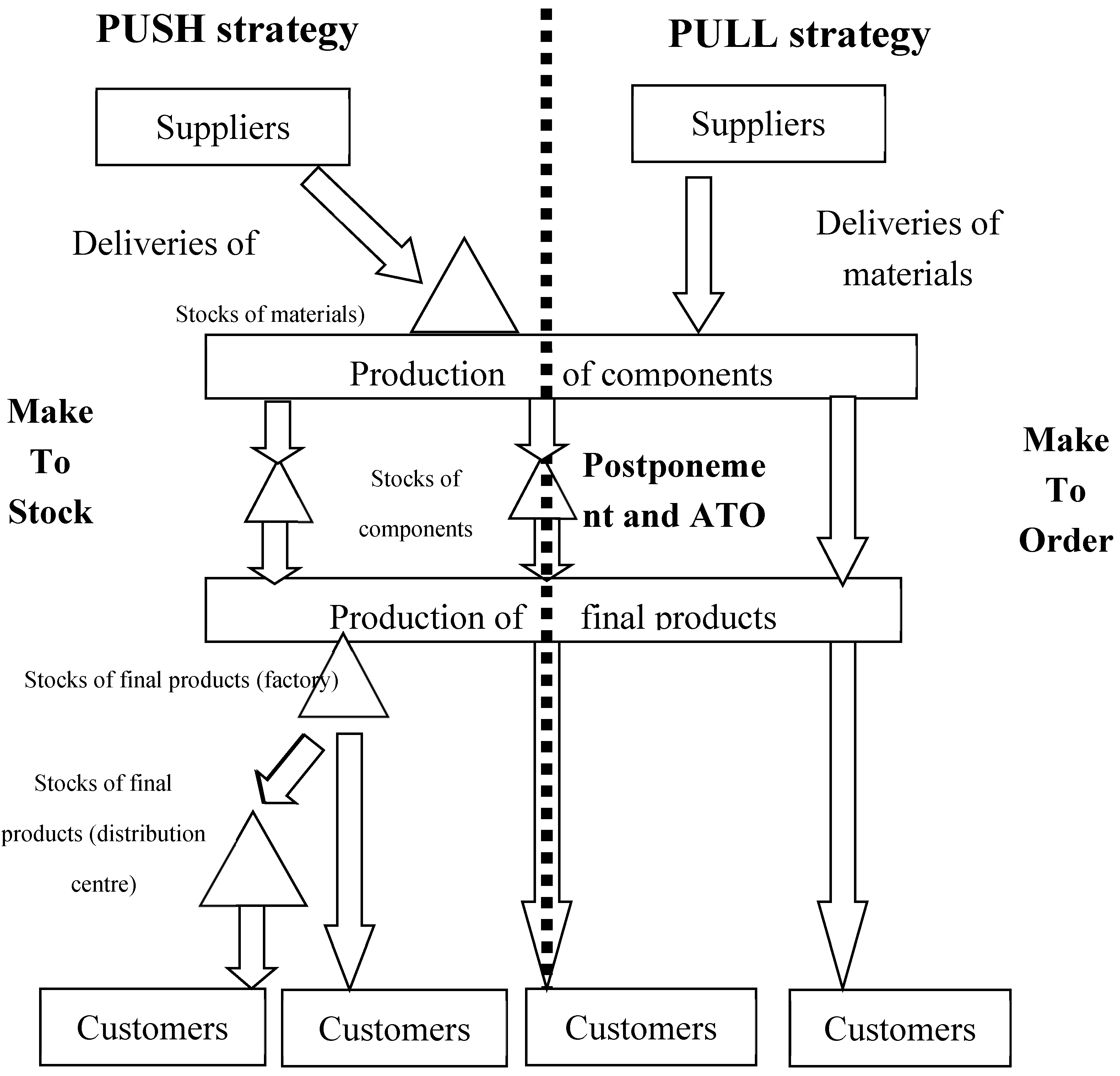
Figure 2.
Applications of .MTS and MTO strategies for different standard and non standard products. Source: author’s own study.
Figure 2.
Applications of .MTS and MTO strategies for different standard and non standard products. Source: author’s own study.
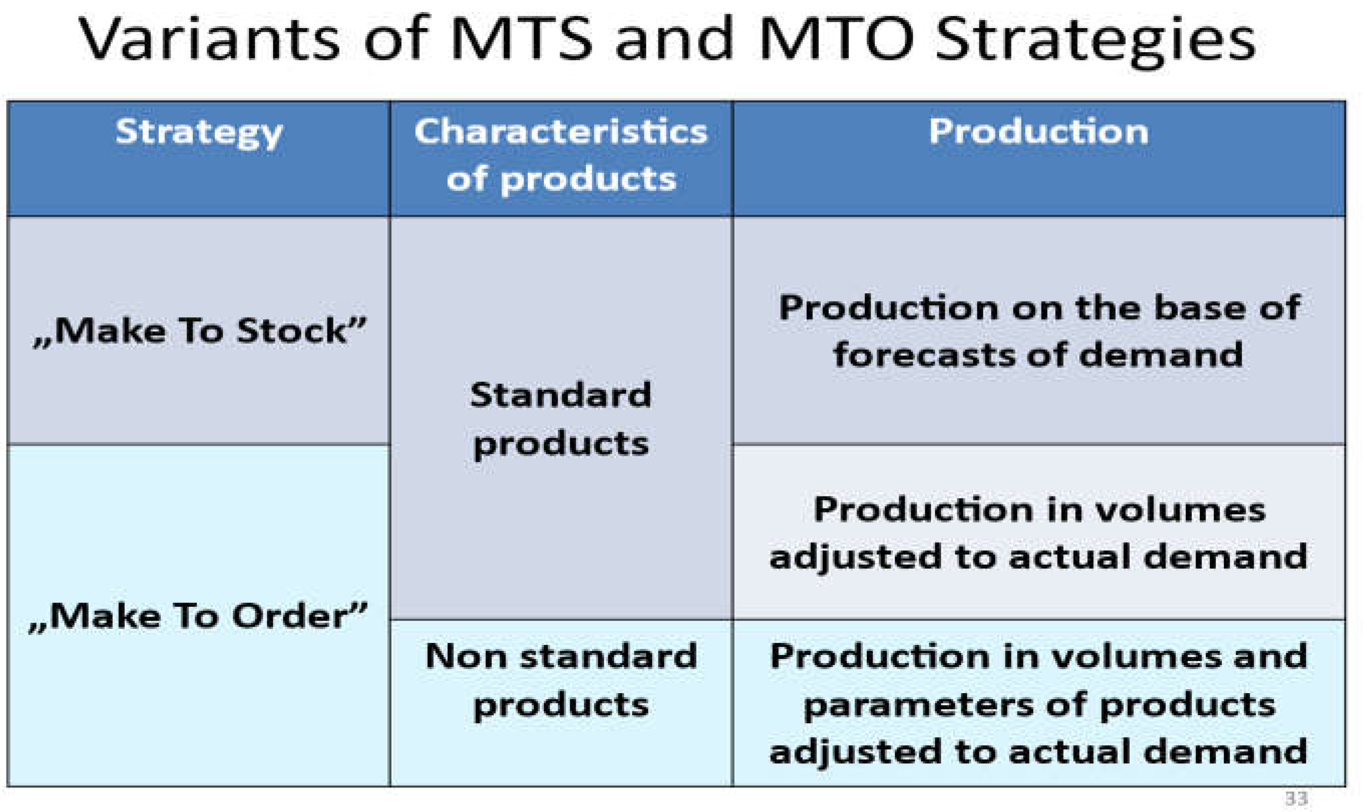
Figure 3.
Availability of stocks in warehouses - 5% of standard deviation of average sales. Different strategies of distribution (Gauss Distribution).
Figure 3.
Availability of stocks in warehouses - 5% of standard deviation of average sales. Different strategies of distribution (Gauss Distribution).
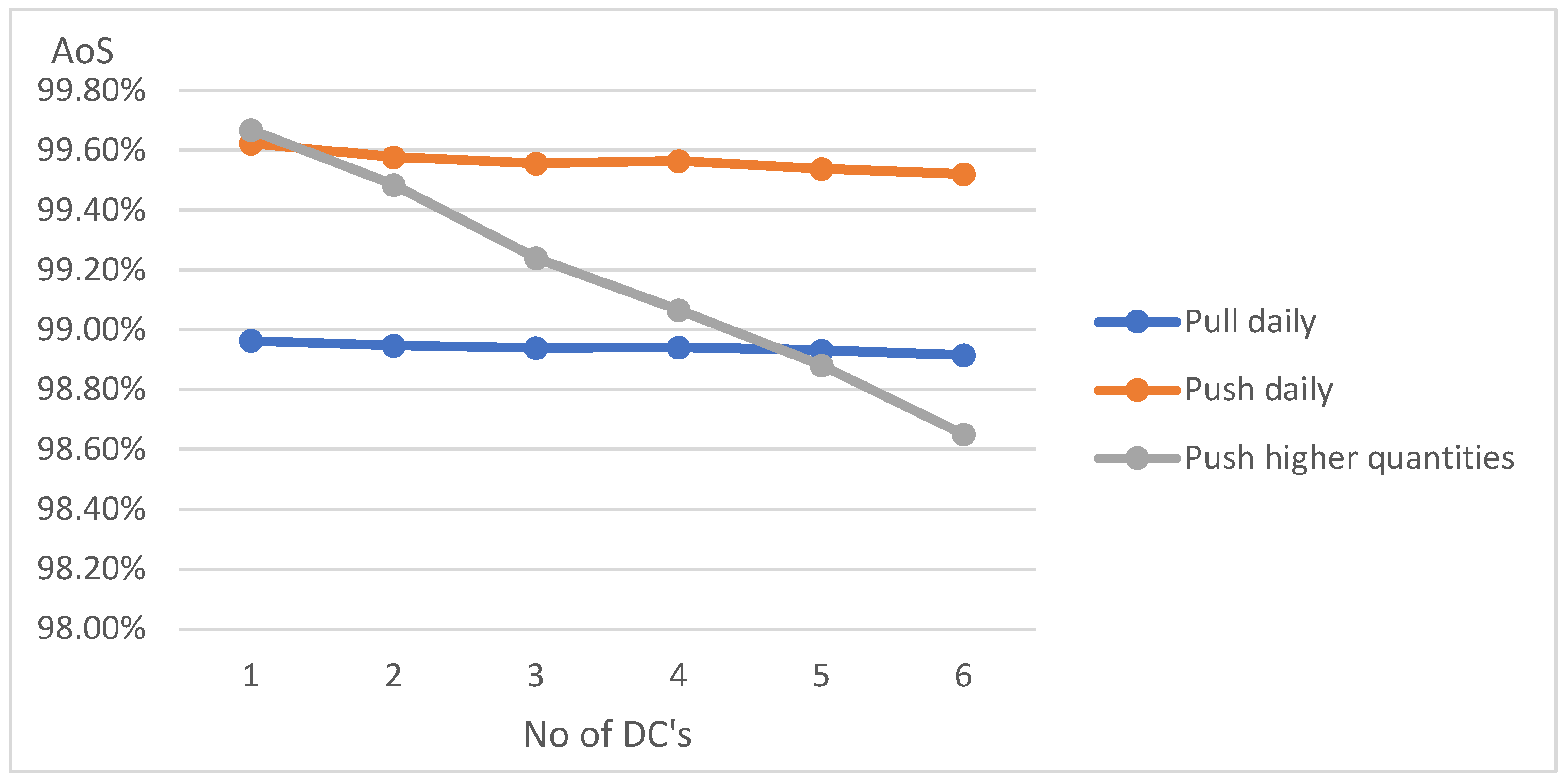
Figure 4.
Availability of stocsks in warehouses - 30% of standard deviation of average sales. Different strategies of distribution (Gauss Distribution).
Figure 4.
Availability of stocsks in warehouses - 30% of standard deviation of average sales. Different strategies of distribution (Gauss Distribution).
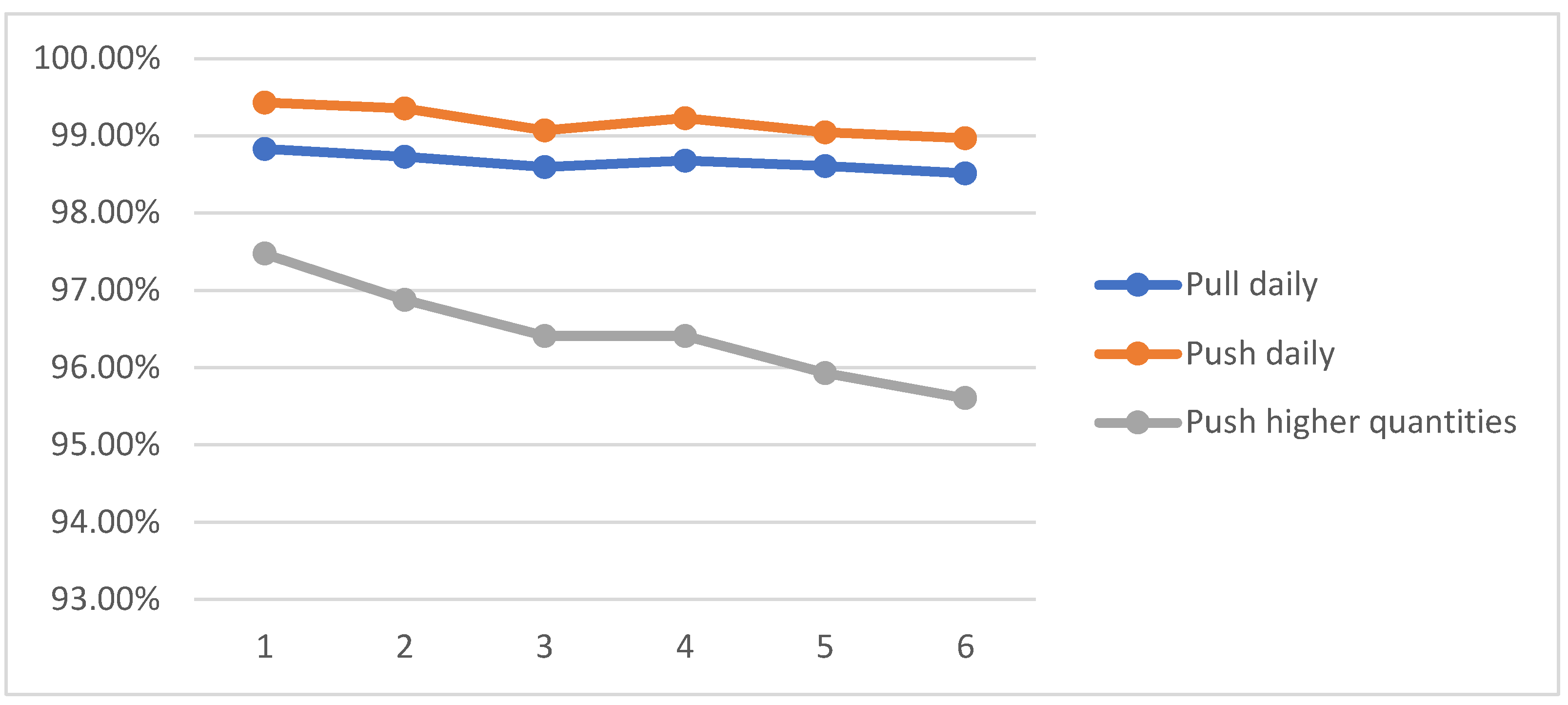
Figure 5.
Level of stocks in warehouses - 5% of standard deviation of average sales. Different strategies of distribution.
Figure 5.
Level of stocks in warehouses - 5% of standard deviation of average sales. Different strategies of distribution.
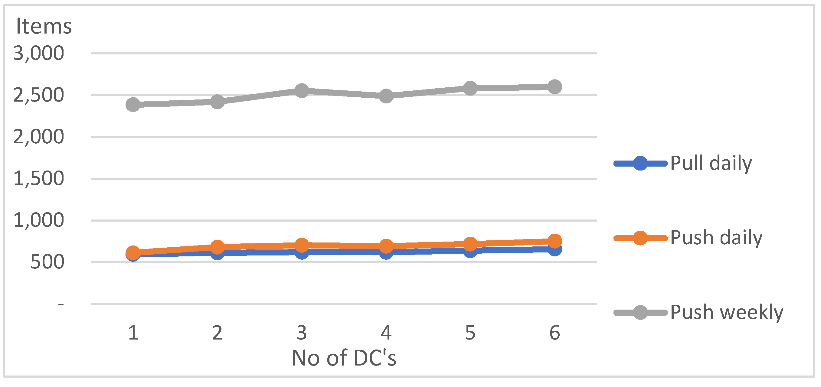
Figure 6.
Level of stocks in warehouses - 3% of standard deviation of average sales. Different strategies of distribution.
Figure 6.
Level of stocks in warehouses - 3% of standard deviation of average sales. Different strategies of distribution.
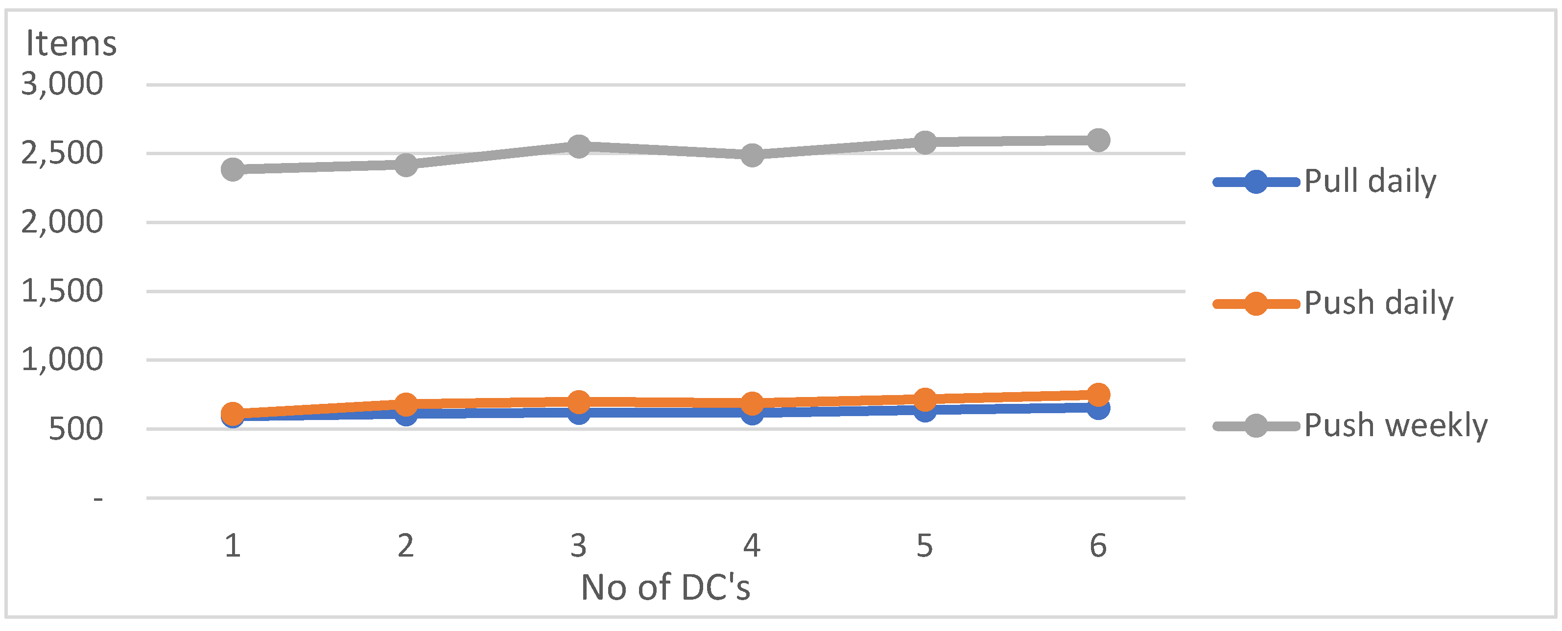
Figure 7.
Level of stocks in warehouses - 5% of standard deviation of average sales. Different strategies of distribution (100% AoS).
Figure 7.
Level of stocks in warehouses - 5% of standard deviation of average sales. Different strategies of distribution (100% AoS).
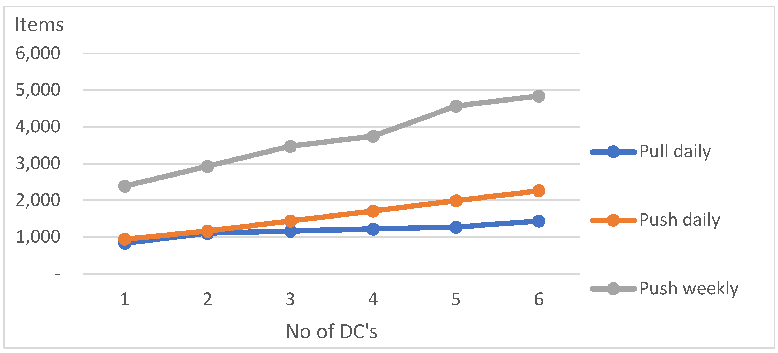
Figure 8.
Level of stocks in warehouses - 5% of standard deviation of average sales. Different strategies of distribution (100% AoS).
Figure 8.
Level of stocks in warehouses - 5% of standard deviation of average sales. Different strategies of distribution (100% AoS).
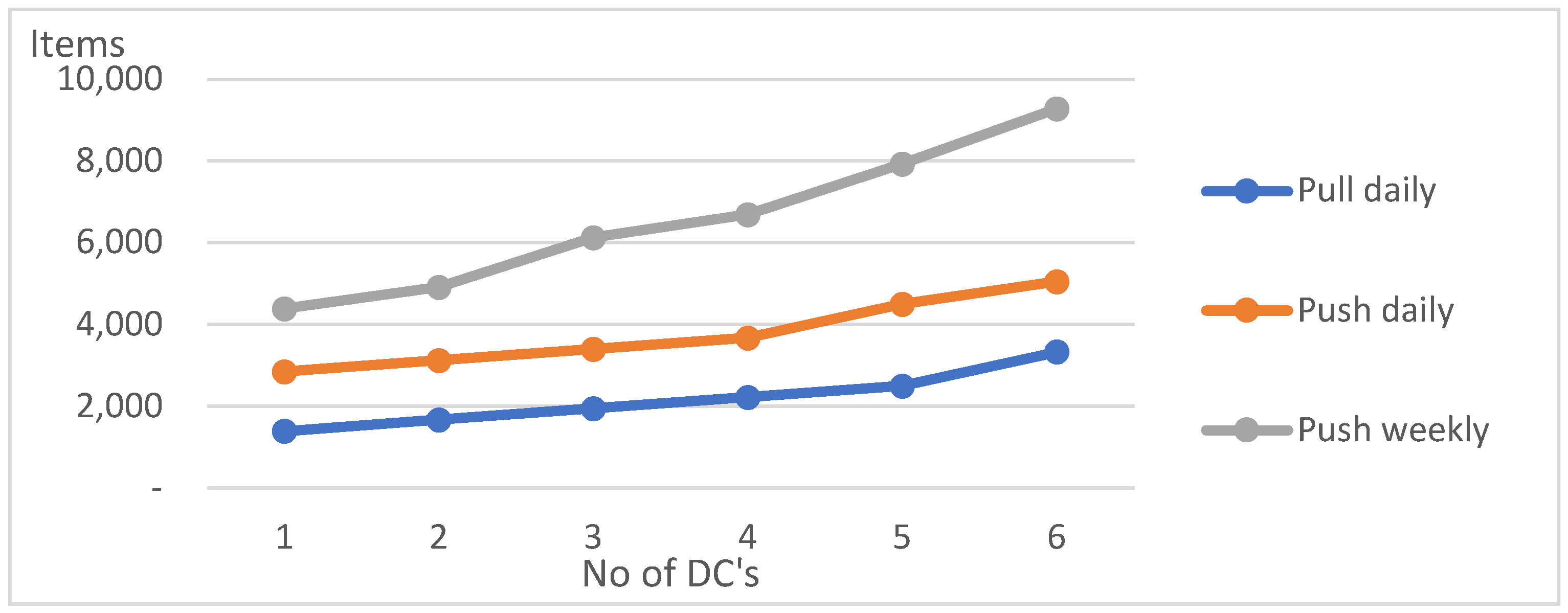
Figure 9.
Availability of stocks in warehouses - 5% of standard deviation of average sales. Different strategies of distribution (Gamma Distribution).
Figure 9.
Availability of stocks in warehouses - 5% of standard deviation of average sales. Different strategies of distribution (Gamma Distribution).
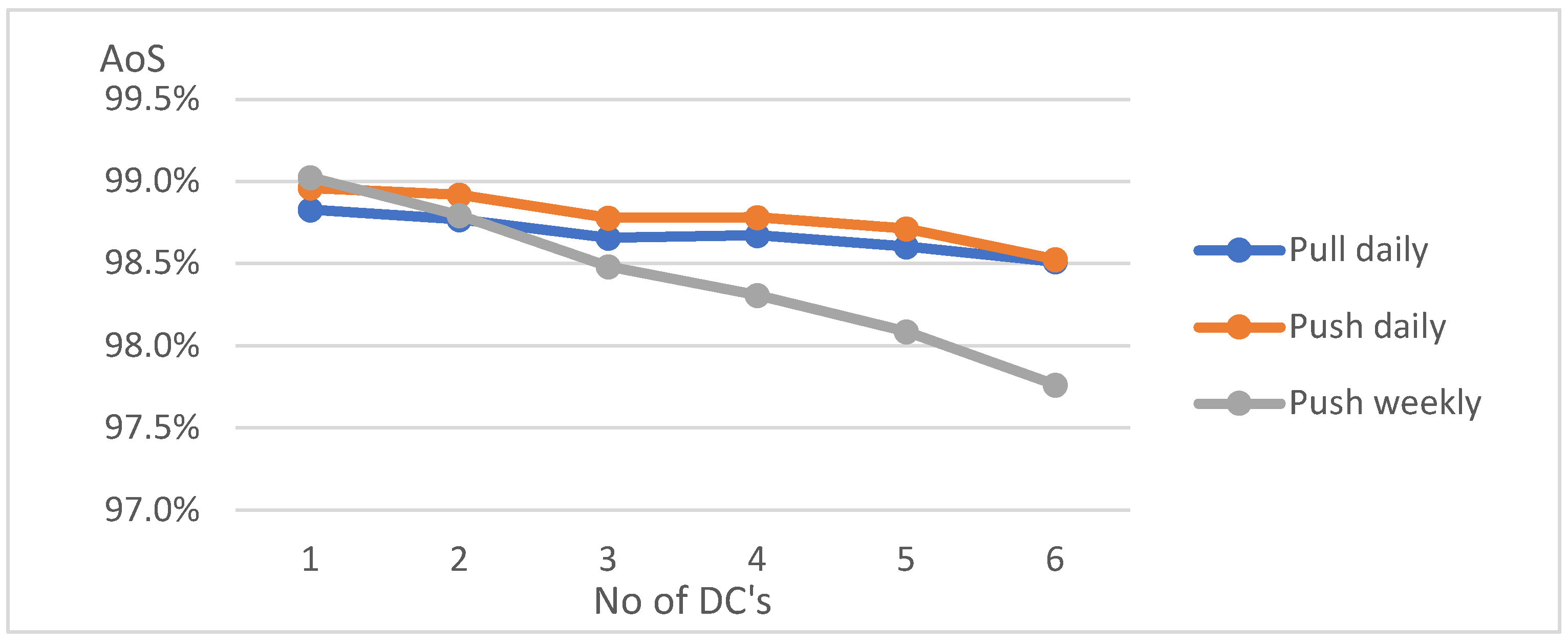
Figure 10.
Availability of stocks in warehouses - 30% of standard deviation of average sales. Different strategies of distribution (Gamma Distribution).
Figure 10.
Availability of stocks in warehouses - 30% of standard deviation of average sales. Different strategies of distribution (Gamma Distribution).
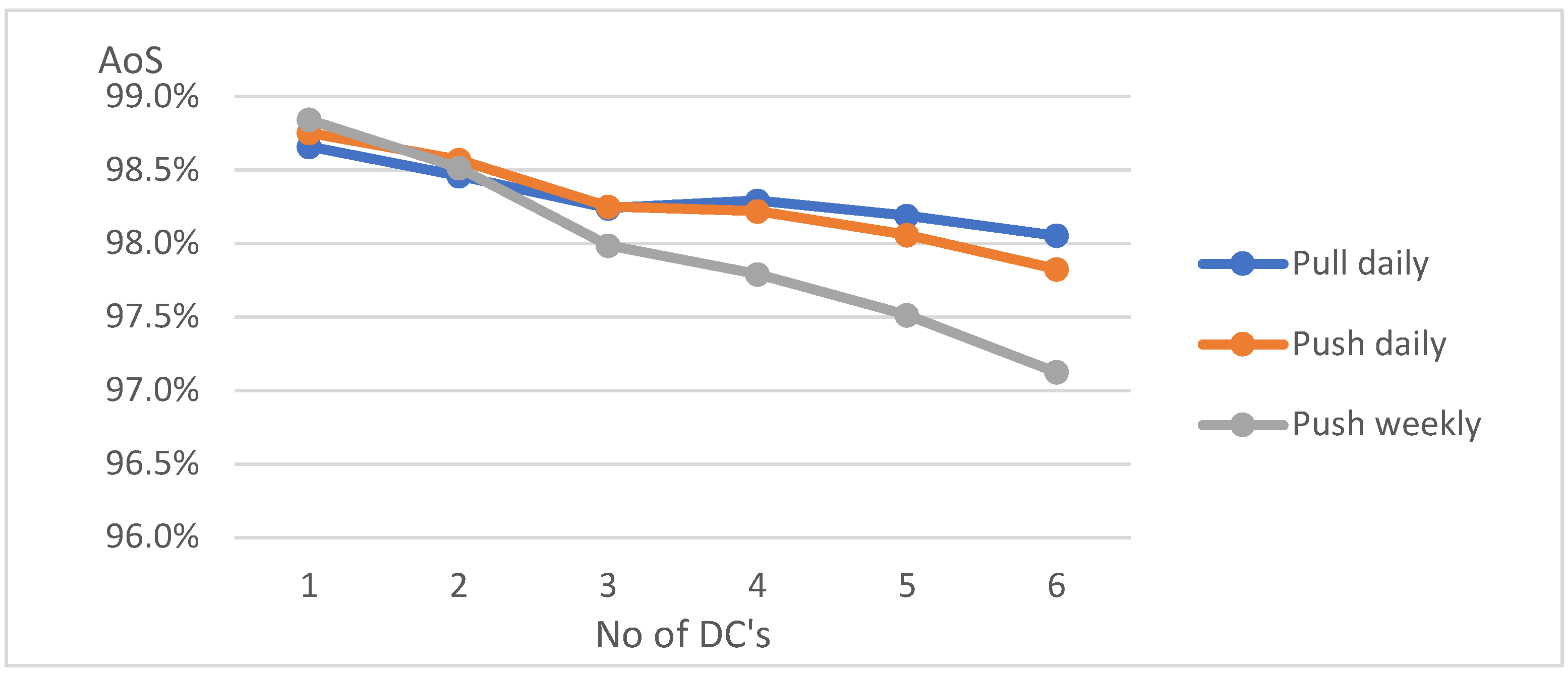

Table 1.
Impact of distribution strategies on the availability of stocks in DC’s (Gauss Distribution). Yearly sales [items/year] = 40000.
Table 1.
Impact of distribution strategies on the availability of stocks in DC’s (Gauss Distribution). Yearly sales [items/year] = 40000.
| Strategy | Stand. dev. of average sales | No of DC’s | |||||
|---|---|---|---|---|---|---|---|
| 1 | 2 | 3 | 4 | 5 | 6 | ||
| Pull daily | 5% | 98, 96% | 98, 95% | 98, 94% | 98, 94% | 98, 93% | 98, 92% |
| Push daily | 5% | 99, 62% | 99, 58% | 99, 56% | 99, 56% | 99, 54% | 99, 52% |
| Push weekly | 5% | 99, 67% | 99, 48% | 99, 24% | 99, 07% | 98, 88% | 98, 65% |
| Pull daily | 30% | 98, 83% | 98, 73% | 98, 59% | 98, 68% | 98, 61% | 98, 51% |
| Push daily | 30% | 99, 43% | 99, 36% | 99, 07% | 99, 23% | 99, 05% | 98, 97% |
| Push weekly | 30% | 97, 47% | 96, 87% | 96, 41% | 96, 41% | 95, 93% | 95, 61% |
Source: Own calculations.
Table 2.
Impact of distribution strategies on the level of inventories [1000 pcs.] (Gauss Distribution). Yearly sales [items/year] = 40000.
Table 2.
Impact of distribution strategies on the level of inventories [1000 pcs.] (Gauss Distribution). Yearly sales [items/year] = 40000.
| Strategy | Stand. dev. of average sales | No of DC’s | |||||
|---|---|---|---|---|---|---|---|
| 1 | 2 | 3 | 4 | 5 | 6 | ||
| Pull daily | 5% | 595 | 610 | 620 | 619 | 637 | 657 |
| Push daily | 5% | 613 | 680 | 700 | 690 | 716 | 752 |
| Push weekly | 5% | 2 385 | 2 418 | 2 553 | 2 488 | 2 582 | 2 598 |
| Pull daily | 30% | 785 | 905 | 995 | 1 030 | 1 137 | 1 242 |
| Push daily | 30% | 925 | 1 267 | 1 608 | 1 383 | 1 728 | 1 894 |
| Push weekly | 30% | 3 329 | 3 658 | 3 986 | 3 807 | 4 366 | 4 816 |
Source: Own calculations.
Table 3.
Impact of distribution strategies on the level of inventories [1000 pcs.] (100% AoS and Gauss Distribution). Yearly sales [items/year] = 40000.
Table 3.
Impact of distribution strategies on the level of inventories [1000 pcs.] (100% AoS and Gauss Distribution). Yearly sales [items/year] = 40000.
| Strategy | Stand. dev. of average sales | No of DC’s | |||||
|---|---|---|---|---|---|---|---|
| 1 | 2 | 3 | 4 | 5 | 6 | ||
| Pull daily | 5% | 831 | 1 106 | 1 161 | 1 216 | 1 271 | 1 437 |
| Push daily | 5% | 944 | 1 164 | 1 438 | 1 713 | 1 987 | 2 262 |
| Push weekly | 5% | 2 390 | 2 923 | 3 472 | 3 746 | 4 569 | 4 843 |
| Pull daily | 30% | 1 390 | 1 667 | 1 944 | 2 221 | 2 498 | 3 330 |
| Push daily | 30% | 2 853 | 3 128 | 3 404 | 3 679 | 4 505 | 5 055 |
| Push weekly | 30% | 4 393 | 4 913 | 6 129 | 6 688 | 7 932 | 9 286 |
Source: Own calculations.
Table 4.
Impact of distribution strategies on the production level and capacity. Yearly sales [items/year] = 40000.
Table 4.
Impact of distribution strategies on the production level and capacity. Yearly sales [items/year] = 40000.
| Strategy | Stand. Dev. of average sales | No of DC’s | |||||
|---|---|---|---|---|---|---|---|
| 1 | 2 | 3 | 4 | 5 | 6 | ||
| Pull daily | 5% | 585 | 585 | 585 | 585 | 585 | 585 |
| Push daily | 5% | 549 | 549 | 549 | 549 | 549 | 549 |
| Push weekly | 5% | 549 | 549 | 549 | 549 | 549 | 549 |
| Pull daily | 30% | 712 | 712 | 712 | 712 | 712 | 712 |
| Push daily | 30% | 554 | 554 | 554 | 554 | 554 | 554 |
| Push weekly | 30% | 551 | 551 | 551 | 551 | 551 | 551 |
Source: Own calculations.
Table 5.
Impact of distribution strategies on the availability of stocks in DC’s (Gamma Distribution) Yearly sales [items/year] = 40000.
Table 5.
Impact of distribution strategies on the availability of stocks in DC’s (Gamma Distribution) Yearly sales [items/year] = 40000.
| Strategy | Stand. dev. of average sales | No of DC’s | |||||
|---|---|---|---|---|---|---|---|
| 1 | 2 | 3 | 4 | 5 | 6 | ||
| Pull daily | 3% | 98, 8% | 98, 8% | 98, 7% | 98, 7% | 98, 6% | 98, 5% |
| Push daily | 3% | 99, 0% | 98, 9% | 98, 8% | 98, 8% | 98, 7% | 98, 5% |
| Push weekly | 3% | 99, 0% | 98, 8% | 98, 5% | 98, 3% | 98, 1% | 97, 8% |
| Pull daily | 6% | 98, 7% | 98, 5% | 98, 2% | 98, 3% | 98, 2% | 98, 1% |
| Push daily | 6% | 98, 8% | 98, 6% | 98, 3% | 98, 2% | 98, 1% | 97, 8% |
| Push weekly | 6% | 98, 8% | 98, 5% | 98, 0% | 97, 8% | 97, 5% | 97, 1% |
Source: Own calculations.
Table 6.
Impact of distribution strategies on the level of inventories [1000 pcs.] (Gamma Distribution). Yearly sales [items/year] = 40000.
Table 6.
Impact of distribution strategies on the level of inventories [1000 pcs.] (Gamma Distribution). Yearly sales [items/year] = 40000.
| Strategy | Stand. dev. of average sales | No of DC’s | |||||
|---|---|---|---|---|---|---|---|
| 1 | 2 | 3 | 4 | 5 | 6 | ||
| Pull daily | 3% | 1 349 | 1 418 | 1 522 | 1 527 | 1 604 | 1 677 |
| Push daily | 3% | 1 443 | 1 550 | 1 732 | 1 727 | 1 856 | 2 071 |
| Push weekly | 3% | 5 229 | 5 927 | 6 166 | 6 515 | 7 222 | 7 736 |
| Pull daily | 6% | 1 507 | 1 784 | 1 872 | 1 910 | 2 069 | 222 |
| Push daily | 6% | 2 586 | 2 926 | 3 241 | 3 220 | 3 520 | 3 778 |
| Push weekly | 6% | 7 543 | 9 135 | 9 058 | 9 183 | 9 991 | 10 837 |
Source: Own calculations.
Table 7.
Impact of distribution strategies on the level of inventories [1000 pcs.] (100% AoS and Gauss Distribution). Yearly sales [items/year] = 40000.
Table 7.
Impact of distribution strategies on the level of inventories [1000 pcs.] (100% AoS and Gauss Distribution). Yearly sales [items/year] = 40000.
| Strategy | Stand. dev. of average sales | No of DC’s | |||||
|---|---|---|---|---|---|---|---|
| 1 | 2 | 3 | 4 | 5 | 6 | ||
| Pull daily | 3% | 843 | 1 114 | 1 170 | 1 225 | 1 283 | 1 447 |
| Push daily | 3% | 2 051 | 2 606 | 2 883 | 3 160 | 3 437 | 3 715 |
| Push weekly | 3% | 5 676 | 7 047 | 8 417 | 10 062 | 11 707 | 12 803 |
| Pull daily | 6% | 1 409 | 1 689 | 2 251 | 2 251 | 2 538 | 3 402 |
| Push daily | 6% | 4 821 | 5 101 | 5 370 | 5 926 | 6 485 | 7 078 |
| Push weekly | 6% | 8 377 | 10 428 | 12 736 | 14 419 | 16 109 | 17 833 |
Source: Own calculations.
Table 8.
Impact of distribution strategies on the production level (Gamma Distribution). Yearly sales [items/year] = 40000.
Table 8.
Impact of distribution strategies on the production level (Gamma Distribution). Yearly sales [items/year] = 40000.
| Strategy | Stand. dev. of average sales | No of DC’s | |||||
|---|---|---|---|---|---|---|---|
| 1 | 2 | 3 | 4 | 5 | 6 | ||
| Pull daily | 3% | 769 | 769 | 769 | 769 | 769 | 769 |
| Push daily | 3% | 554 | 554 | 554 | 554 | 554 | 554 |
| Push weekly | 3% | 548 | 548 | 548 | 548 | 548 | 548 |
| Pull daily | 6% | 955 | 955 | 955 | 955 | 955 | 955 |
| Push daily | 6% | 561 | 561 | 561 | 561 | 566 | 566 |
| Push weekly | 6% | 559 | 559 | 559 | 559 | 559 | 559 |
Source: Own calculations.
Table 9.
Assumptions and input data for calculations of economical effectiveness.
| Commodity | Food | Garment | Electronics |
|---|---|---|---|
| No of items [pcs./year] | 32 000 000 | 2 000 000 | 3 200 000 |
| Weight of a commodity [kg/item] | 1, 00 | 2, 00 | 3, 00 |
| Weight of a commodity [tonnes/pellet] | 0, 80 | 0, 10 | 0, 24 |
| Value of a commodity [EUR/item] | 0, 6 | 18 | 30 |
| Price of a commodity [EUR/item] | 1 | 30 | 50 |
| Transport costs [EUR/tonne/km] - 6 CD’s | |||
| Road transport (PULL) | 0, 069 | 0, 556 | 0, 232 |
| Road transport (PUSH) | 0, 066 | 0, 529 | 0, 221 |
| Rail transport (PUSH) | 0, 013 | 0, 106 | 0, 044 |
| Distances [km] | 800 | 800 | 800 |
| Costs of keeping stocks | |||
| Capital costs in invetories | 10% | 10% | 10% |
| Warehousing [EUR/item/day] | 0, 001 | 0, 020 | 0, 013 |
Source: Own assumptions.
Table 10.
Costs of distribution of different strategies (Food) [thous. EUR/year].
| No of DC’s | 1 | 1 | 6 | 6 | 6 |
| Strategy | Pull daily | Push daily | Pull daily | Push daily | Push weekly |
| Stand. dev. of sales | 5% | ||||
| AoS | 98, 96% | 99, 62% | 98, 92% | 99, 52% | 98, 65% |
| Warehousing&Inv. | 243 | 250 | 268 | 307 | 1 060 |
| Transport | 2 380 | 2 267 | 1 779 | 1 694 | 339 |
| Lost sales | 332 | 121 | 347 | 153 | 432 |
| Total costs | 2 955 | 2 638 | 2 394 | 2 154 | 1 831 |
| Stand. Dev. of sales | 30% | ||||
| AoS | 98, 8% | 99, 4% | 98, 5% | 99, 0% | 95, 6% |
| Warehousing&Inv. | 320 | 377 | 507 | 773 | 1 965 |
| Transport | 2 380 | 2 267 | 1 779 | 1 694 | 339 |
| Lost sales | 374 | 182 | 476 | 330 | 1 406 |
| Total costs | 3 075 | 2 827 | 2 761 | 2 797 | 3 709 |
Source: Own assumptions.
Table 11.
Costs of distribution of different strategies (Garment) [thous. EUR/year].
| No of DC’s | 1 | 1 | 6 | 6 | 6 |
| Strategy | Pull daily | Push daily | Pull daily | Push daily | Push weekly |
| Stand. dev. of sales | 5% | ||||
| AoS | 98, 96% | 99, 62% | 98, 92% | 99, 52% | 98, 65% |
| Warehousing&Inv. | 268 | 276 | 296 | 338 | 1 169 |
| Transport | 2 380 | 2 267 | 1 779 | 1 694 | 339 |
| Lost sales | 622 | 226 | 651 | 287 | 810 |
| Total costs | 3 270 | 2 769 | 2 725 | 2 320 | 2 318 |
| Stand. Dev. of sales | 30% | ||||
| AoS | 98, 8% | 99, 4% | 98, 5% | 99, 0% | 95, 6% |
| Warehousing&Inv. | 353 | 416 | 559 | 853 | 2 167 |
| Transport | 2 380 | 2 267 | 1 779 | 1 69 | 339 |
| Lost sales | 701 | 342 | 892 | 619 | 2 635 |
| Total costs | 3 435 | 3 025 | 3 230 | 3 166 | 5 141 |
Source: Own assumptions.
Table 12.
Costs of distribution of different strategies (Electronic) [thous. EUR/year].
| No of DC’s | 1 | 1 | 6 | 6 | 6 |
| Strategy | Pull daily | Push daily | Pull daily | Push daily | Push weekly |
| Stand. dev. of sales | 5% | ||||
| AoS | 98, 96% | 99, 62% | 98, 92% | 99, 52% | 98, 65% |
| Warehousing&Inv. | 357 | 368 | 394 | 451 | 1 559 |
| Transport | 2 380 | 2 267 | 1 779 | 1 694 | 339 |
| Lost sales | 1 658 | 603 | 1 735 | 766 | 2 159 |
| Total costs | 4 396 | 3 238 | 3 908 | 2 911 | 4 056 |
| Stand. Dev. of sales | 30% | ||||
| AoS | 98, 8% | 99, 4% | 98, 5% | 99, 0% | 95, 6% |
| Warehousing&Inv. | 471 | 555 | 745 | 1 137 | 2 889 |
| Transport | 2 380 | 2 267 | 1 779 | 1 694 | 339 |
| Lost sales | 1 870 | 911 | 2 379 | 1 651 | 7 028 |
| Total costs | 4 722 | 3 733 | 4 902 | 4 482 | 10 256 |
Source: Own assumptions.
Disclaimer/Publisher’s Note: The statements, opinions and data contained in all publications are solely those of the individual author(s) and contributor(s) and not of MDPI and/or the editor(s). MDPI and/or the editor(s) disclaim responsibility for any injury to people or property resulting from any ideas, methods, instructions or products referred to in the content. |
© 2025 by the authors. Licensee MDPI, Basel, Switzerland. This article is an open access article distributed under the terms and conditions of the Creative Commons Attribution (CC BY) license (http://creativecommons.org/licenses/by/4.0/).
Copyright: This open access article is published under a Creative Commons CC BY 4.0 license, which permit the free download, distribution, and reuse, provided that the author and preprint are cited in any reuse.


