Submitted:
19 February 2025
Posted:
20 February 2025
You are already at the latest version
Abstract
Feature selection from data is a pivotal area within machine learning, statistics, and artificial intelligence. Given the lack of a unified concept so far, numerous methodologies have been introduced to address this challenge. Recently, the Shapley value has gained traction for feature selection, driven partly by its accomplishments in explainable AI and interpretable machine learning. This paper aims to explore feature selection using the Shapley value, comparing it with established methods. Specifically, we conduct a comparative analysis of 14 distinct feature selection methods by studying their performance across four datasets representing three diverse data types. As a result, we find that Shapley value-based feature selection is competitive to the best methods from the literature, including Minimum Redundancy Maximum Relevance and Predictive Permutation Feature Selection, but not under all conditions. Furthermore, our analysis sheds light on some more fundamental aspect by demonstrating that there is no feature selection method that dominates all others for all data. Also, application of feature selection seems not necessarily beneficial for all data.
Keywords:
feature selection
; prediction model
; data science
; classification
1. Introduction
Data science and machine learning models for high-dimensional data frequently employ feature selection methods [8,39]. Feature selection, also known as variable selection or variable subset selection, involves choosing a relevant subset of features for further analysis, such as in classification or regression models. Feature selection is motivated by several factors, including reducing computational training costs, preventing overfitting, eliminating irrelevant or redundant features, and simplifying models to enhance interpretability [29,47]. Interestingly, the pursuit of interpretability is closely linked to explainable artificial intelligence (XAI) [1,21]. Unfortunately, feature selection introduces an additional layer of complexity to the overall problem since finding the optimal feature set within the feature space is a challenging task.
Over the last decades, numerous feature selection methods have been introduced [52,56]. Importantly, several approaches that came recently into spotlight are exploiting a framework based on Shapely value [48], spurred partly due to its success in explainable AI and interpretable machine learning [25]. While the earliest use of Shapely value for feature selection dates back to 2007 [13], recent studies introduced extended methods [10,60]. These studies show promising results but lack a more comprehensive analysis. In this paper, we aim to fill this gap by investigating the functionality of Shapely value for feature selection of two approaches: Shapley value feature selection (SHAP) [34] and Interaction Shapely Value (ISV) [11]. In order to gain comprehensive insights, we compare SHAP and ISV with well-established feature selection methods. In total, we compare 14 different feature selection methods (FSM) for 4 different datasets. The methods include 10 filtering approaches (Term Strength (TS) [2], Mutual Information (MI) [57], Joint Mutual Information (JMI) [59], Maximum Relevance and Minimum Redundancy feature selection (mRMR) [46], (Chi-squared test) [5], Term ReLatedness (TRL) [6], Entropy-based Category Coverage Difference (ECCD) [38], Linear Measure (LM) [14], F-stat [9,19] and Class-based term frequency–inverse document frequency (c-TF-IDF) [33] and 4 wrapper methods (Linear Forward Search (LFS) [27], Predictive Permutation Feature Selection (PPFS) [30], Shapley value-based feature selection (SHAP) [34]) and Interaction Shapely Value (ISV) [11].
In addition, our paper aims to enhance our general understanding of feature selection. Importantly, one needs to distinguish between theoretical considerations and practical realizations. While, ideally, an optimal feature selection method would be able to find the Markov blanket, i.e., a subset of features that carries all information providing causal relations among covariates [24,36,45,61], practically, this goal is very difficult to achieve. A reason therefor is that available data have always a finite sample size and may be corrupted by measurement errors. Furthermore, data may be incomplete by not including all relevant features. All of those issues may be present for a given dataset but usually we lack detailed information. To obtain insights about this and related problems, we include Predictive Permutation Feature Selection (PPFS) [30] in our analysis that aims to estimate the Markov blanket. We study also the very popular approach called Maximum Relevance and Minimum Redundancy (mRMR) [46]. While mRMR does not directly target conditional independence, it indirectly relates to it by encouraging the selection of features that exhibit minimal redundancy, which is conducive to the notion of conditional independence. In contrast, most other approaches we are studying, including SHAP and ISV, are more heuristic with respect to their underlying working mechanisms. Hence, a comparison between such different methods will allow to evaluate their practical functioning under different conditions.
This paper is organized as follows. In the next section, we review related work and specify our research questions. The next section discusses the methods and the data we use for the analysis. Then we present our numerical results. The paper finishes with a discussion and concluding remarks.
2. Research Questions
Despite the extensive literature about feature selection, there are a number of open questions, partly informed by recent developments in explainable AI. Specifically, in this paper, we aim to study the following main questions.
- Can Shapley-value be used for a reliable and robust selection of feature?
- Are complex feature selection methods (for instance, PPFS or mRMR) are always better than less complex methods (, F-stat or SHAP)?
- Is there an optimal feature selection method that performs best under all conditions?
- Is feature selection always beneficial?
3. Methods
In this section, we discuss briefly all 14 feature selection methods we use for our analysis. Furthermore, we describe four datasets for our numerical analysis.
3.1. Filter Methods
In this section, we describe 10 filtering approaches: Term Strength (TS) [2], Mutual Information (MI) [57], Joint Mutual Information (JMI) [59], Maximum Relevance and Minimum Redundancy (mRMR) [46], (chi2) [5], Term ReLatedness (TRL) [6], Entropy-based Category Coverage Difference (ECCD) [38], Linear Measure (LM)[14], F-stat [9,19] and Class-based term frequency–inverse document frequency (c-TF-IDF) [33].
3.1.1. Term Strength (TS)
Term strength is a filtering feature selection technique initially developed for stop-word removal in an unsupervised fashion, used to measure how informative a word is for identifying two related documents [3]. For two related documents x and y, the term strength of term t is defined as the following conditional probability. Formally, term strength can be estimated via a Maximum Likelihood Estimation (MLE) for a multinomial distribution [2]. The actual feature selection can be implemented with pruning terms based on their estimated strength by comparing terms’ strength to the expected strength of a random term [3].
3.1.2. Mutual Information (MI)
Mutual information (MI) is a measure of the amount of information that one random variable contains about another variable [57]. It is useful in the context of feature selection as it gives a measure of the relevance between a feature and another variable of interest. If x and y are independent random variables, then . MI can be efficiently estimated, see, e.g., [37].
3.1.3. Joint Mutual Information (JMI)
Mutual information gives the relevance of a single feature but does not consider a redundancy between the features. Joint Mutual Information (JMI) [59] allows to define the relevance of a set of features instead.
The Conditional Mutual Information (CMI) measures the information gain obtained by including one additional variable to a set. Given a set of already selected variables, S, and a variable to be added , the Conditional Mutual Information is defined as [59]:
If and y are conditionally independent given , then CMI of and y given the rest of the features will be equal to zero, and will not provide any additional information to a model which means is redundant.
3.1.4. Maximum Relevance and Minimum Redundancy (mRMR)
Maximum Relevance and Minimum Redundancy (mRMR) [46] is a very popular feature selection method that extends mutual information based approaches to combat redundancies in the resulting feature subset. The mRMR algorithm aims to approximate the maximum dependency between a feature subset S with an incremental optimization algorithm, which should maximize relevance and minimize redundancy within the feature subset. Maximum dependency itself is extremely hard to calculate as it requires computing two multivariate joint probability density functions: joint probability density function of all features within subset S and target variable c called and joint probability density function of all feature in S called .
3.1.5. (Chi-Squared Test)
is a test statistic used to examine whether two discrete variables are independent. Intuitively, a statistic is higher for features that are differently distributed across different classes. between the feature and class is defined as [5]:
where N is the total number of documents in the corpus, A is the number of documents in class that contain the term ; B is the number of documents that contain the term in other classes; C is the number of documents in class that do not contain term ; D is the number of documents that do not contain term in other classes.
3.1.6. Term ReLatedness (TRL)
Term ReLatedness (TRL) is a feature selection approach that aims at sorting terms in order of their usefulness for each category [6]. The following evaluation function was proposed to maintain the preference ordering of the terms:
with
Here is the probability that a document contains term t and is the probability that a document belongs to category . is the probability that a document belongs to category and contains the term t and is the probability of a document not belonging to category and containing term t; and is the Shannon entropy of category . The values of , and are normalized to be within . The resulting feature importance measure is the minimum of across all categories.
3.1.7. Entropy-Based Category Coverage Difference (ECCD)
The Entropy-based Category Coverage Difference (ECCD) is a feature selection criterion that exploits two hypotheses to evaluate the usefulness of a term for document categorization. The first hypothesis states that a term is useful if the major part of the documents containing that term belongs to the category of interest. The other hypothesis assumes that the number of occurrences of the term in the documents belonging to the category should be high and it must be lower in the documents belonging to all the other categories [38].
ECCD is defined as follows:
where is the probability of observing the word in a document belonging to the category and is respectively the probability of observing in all other categories. The ECCD provides feature importance values per classification category, hence, the terms are filtered by their maximum ECCD value across all categories.
3.1.8. Linear Measure-Based Methods (LM)
Linear Measure-based methods assume an association between each pair of a word w and a category c by the following rule: “If the word w appears in the document, then that document belongs to category c”. This is denoted by . The proposed families of measures are used to evaluate the quality of this rule and to select the most promising words for text classification.
Let denote the number of documents of the category c in which the word w appears. Correspondingly denotes the number of documents that contain the word w, but does not belong to the category c. With this definition, a linear filtering measure is defined as follows [14]:
where k is the family parameter. As a special case, for we obtain:
which is the family of linear measures.
3.1.9. F-Statistic Based Feature Selection (F-Stat)
A F-statistic is widely used for feature selection method used for classification problems, e.g., [9,19]. In general, a F-test in a one-way analysis of variance (ANOVA) is used to evaluate whether the means of continuous variables within two or more classes/groups differ from each other. The meaning of a F-statistic is the “between-class variability/within-class variability” and the resulting F-statistic follows a F-distribution. By evaluating the F-statistic for each feature allows to estimate p-values for features. These p-values are then used to rank the features and thresholding allows to make a selection of features.
3.1.10. Class-Based Term Frequency—Inverse Document Frequency (c-TF-IDF)
The c-TF-IDF method [33] is an extension of TF-IDF (term frequency–inverse document frequency), where TF-IDF values are calculated on the class-level instead of the document-level. A high value in TF-IDF is obtained by a high term frequency in the given document, but a low document frequency of the term in the whole corpus. Intuitively, it means that a term has good predictive power according to TF-IDF if it frequently appears in a small subset of documents, which are usually of the same category.
Class-based TF-IDF aggregates all documents within the same class and applies the same logic TF-IDF has. Resulting c-TF-IDF values show terms weights not from a document, but class perspective, i.e., high c-TF-IDF value means that a term is frequent in one class and rarely appears in the rest of the classes, hence it has good discriminatory power in the categorization task. Formally c-TF-IDF is defined as [33]:
where stands for frequency of each term t extracted for each class i, is the total number of words w in the class i, m is the total number of documents before the aggregation and is the total frequency of term t across all n classes. c-TF-IDF produces separate word weightings for each class. Feature importance values for each term can be obtained by taking the maximum weight across all classes.
3.2. Wrapper Methods
In this section, we discuss the 4 wrapper methods (Linear Forward Search (LFS) [27], Predictive Permutation Feature Selection (PPFS) [30], Shapley value feature selection (SHAP) [34] and Interaction Shapley Value feature selection (ISV) [11].
3.2.1. Linear Forward Search (LFS)
Linear Forward Search (LFS) is a technique that allows limiting the number of attribute expansions during each feature addition or removal step [27]. In order to reduce the number of expansions LFS uses external feature ranking, i.e., a ranking produced by another method, e.g., a filter feature selection method. This allows the algorithm at each step to restrict the search space to the k best features according to the ranking. There are two common ways to construct the feature space called fixed set and fixed width. With the fixed set method, the set of available features for consideration is fixed at the very beginning. This is equivalent to running Sequential Feature Selection only on the k best features according to the ranking. In contrast, fixed width maintains the same number of features k for a possible expansion at each step by adding the next best ranked feature to the set after each step. That means at every point k features are considered. For large enough k and , where is the total number of features available, the difference in performance between fixed set and fixed width is negligible. The Linear Forward Search is a greedy search method and therefore cannot guarantee to find the optimal solution.
3.2.2. Predictive Permutation Feature Selection (PPFS)
Predictive Permutation Feature Selection (PPFS) [30] is a novel wrapper-based feature selection method that directly estimates the Markov Blanket of a target variable. PPFS can handle different feature-types and different prediction tasks, i.e., both regression and classification, unlike more traditional Markov-Blanket-based approaches.
All Markov-Blanket-based feature selection approaches rely on conditional independence (CI) tests in order to verify that deselected features are conditionally independent of the target variable given the discovered Markov Blanket. Traditional filter-based feature selection techniques use different statistical hypothesis tests for different feature and target data types [44]. Importantly, PPFS uses the Predictive Permutation Independence (PPI) test, which is both target and feature data type agnostic.
The PPI test is built on top of the knockoff framework. The main idea behind the knockoff framework is that in order to be important a feature must be able to perform significantly better than its knockoff counterpart. Knockoff counterpart feature is defined as a row permutation of the feature, i.e., rows of the feature are shuffled to break the relationship between features and the target variable.
3.2.3. Shapley Value-Based Feature Selection (SHAP)
Shapley value is a concept from cooperative game theory, that defines a fair payoff in a game. The game can be defined as follows [34]. Let N be the set of n players and v be some real-valued function that takes in a subset of the players and returns the payoff of the game for the corresponding subset. The Shapley value of a feature i is defined by
where N be the set of n players and v be some real-valued function that takes values in a subset of the players and returns the payoff of the game for the corresponding subset and S is a subset of players participating in each variation of the game.
Shapley values find a direct application in machine learning. In this context, the machine learning model can be viewed as a cooperative game, where v represents the model’s output and the players represent the features used in the model. With this conceptualization, Shapley values offer insight into the marginal contribution of each feature. Moreover, calculating the mean of the absolute Shapley values across the entire dataset can be regarded as feature importance values [40,41]. Due to the fact that Shapley value-based feature selection require the training of the machine learning model for every possible feature subset, such an approach is a wrapper method. Usually, this is very time consuming but in [41] an efficient approximation has been introduced to estimate Shapley values for trees (for instance random forests) with a polynomial-time algorithm.
The naive version of the Shapley value-based feature selection we call SHAP is defined in Algorithm 1 [34].
| Algorithm 1: Shapley value feature selection (SHAP) |
|
3.2.4. Interaction Shapley Value (ISV)
The Interaction Shapley Value (ISV) feature selection method [11] extends the naive Shapley value algorithm discussed above by eliminating contributions from features that are not in the selected feature subset. ISV directly mitigates two consequences from the Shapley value axioms: model averaging and redundancy from symmetry. This is achieves by considering separate feature contributions and iteratively adding features with the most additional contributions.
The ISV algorithm relies heavily on the Boosted Trees model and SHAP library [40]. This combination allows to compute both Shapley values and pairwise feature interaction effects in polynomial time. ISV requires only one model training to obtain the required feature interactions. ISV implementation is described in Algorithm 2
| Algorithm 2: Interaction Shapley Value feature selection (ISV) |
|
The ISV algorithm is essentially a model-dependent greedy search algorithm. Its computational complexity is , where M is the total number of features in the dataset and K is the number of selected features. The main limitation of ISV is its memory requirements which needs memory that is proportional to . Hence, for very large M (total number of features) as needed, e.g., for text data, the usage of the ISV algorithm can become impossible.
3.3. Data
For our analysis, we use four different benchmark datasets. The data can be categorized into three different data-types: Text data (Enron and Brown), mass-spectrometry data (Arcence) and radar signals (Ionosphere).
3.3.1. Enron Data
The Enron data for spam detection [55] contain emails collected during the Enron bankruptcy investigation. It was the first major dataset with real emails. Originally, the Enron corpus contains over emails, however, with unbalanced classes. To simplify the task, we sub-sample the data to obtain approximately balanced classes between spam and non-spam messages. For our analysis, we use samples for spam and samples for non-spam emails. After preprocessing the corpus contains unique tokens we use as features.
3.3.2. Brown Data
The Brown corpus is the first million-word electronic corpus in English language [22]. The corpus contains 500 documents belonging to 15 genres where one document can only belong to one genre. We use the Brown corpus for multi-class, single-label classification, i.e., only one genre can be assigned to any given document. Interestingly, each document is rather long, containing at least 2000 words. After preprocessing, the Brown corpus contains unique tokens used as features.
3.3.3. Arcene Data
The Arcene data contains three merged mass-spectrometry datasets measured with SELDI (Surface-enhanced laser desorption/ionization) from cancer and from normal (control) patterns [28]. Cancer can be either ovarian or prostate cancer. Features indicate the abundance of proteins having a given mass value. The original dataset was used for the NIPS 2003 feature selection competition and consists of 7000 actual features and 3000 artificially added distractor features. All features are real-valued. Available samples are as follows: Training set: 44 positive examples, 56 negative examples (total 100), Validation set: 44 positive examples, 56 negative examples (total 100), Test set: 310 positive examples, 390 negative examples (total 700), Overall: 398 positive examples, 502 negative examples (total 900).
3.3.4. Ionosphere Data
The Ionosphere dataset comprises 351 Instances and 34 features [49]. The radar data were collected by a system located in Goose Bay, Labrador. This system consists of a phased array of 16 high-frequency antennas with a total transmitted power of approximately 6.4 kilowatts. The targets were free electrons in the ionosphere and “good” radar returns are those that show evidence of some type of structure in the ionoshpere whereas all others are considered “bad”. For our analysis of the Ionoshpere data, we use 225 samples for “good” and 126 samples for “bad”.
4. Results
In this section, we show numerical results for 14 feature selection methods and 4 datasets where the following subsections are structured according to the datasets. For all results, the baseline model shown in the figures corresponds to a classifier using all features. That means, the baseline model is a classifier without feature selection. The standard errors are estimated using a 5-fold cross-validation (CV).
4.1. Enron Spam Detection
For performing spam detection with text data from Enron, we use a Support Vector Machine (SVM) for a binary classification. That means each instance, corresponding to an email, is either classified as spam or non-spam email. The Enron dataset a very high-dimensional consisting of features.
The results of the analysis are shown in Figure 1 where the top figure shows results for the training data and the bottom figure for the test data. From this one can see that all feature selection methods except Term ReLatedness (TRL) converge around 3000 features. For the test data, the best performance is achieved for the Shapley value-based feature selection (SHAP) but other methods perform similarly well, including Term Strength (TS) and Mutual Information (MI). Interestingly, the baseline model that used all available features performs also very well.
In Table 1, we show Jaccard scores between SHAP and the 7 feature selection methods from Figure 1 for different numbers of features. As one can see, the highest observable overlap is 50.5% between SHAP and LM for 1000 features. Similar values are observed for TS, TF-IDF and . In general, for small feature sets the overlap is higher than for large feature sets for all feature selection methods. For 3000 features, for smallest overlap is with TRL and ECCD. This is interesting because TRL performs very poorly (see Figure 1) while the performance of ECCD is similar to SHAP. This indicates that a small overlap is no indicator of large performance changes between the feature selection methods but shows that there is a lot of redundancy in the features/words, so it is possible to pick different features while maintaining a high performance.
Table 2 shows the Jaccard scores between all tested methods for 3000 features/words, where the best performance was achieved. Overall, the overlap between TRL and all other methods is lowest followed by SHAP. Interestingly, all other methods have a higher overlap with each other. For instance, the overlap between LM and TS is 96.3% and between and MI 89.5%. These are very high values considering the each of those feature selection methods is based on a different methodology.
We want to mention that Linear Forward Search (LFS) is not shown in this or any other analysis due to its slowness. Considering that it has to train models, where k is the number of features to be consider during each feature expansion and n is the total number of features/words, it is simply impractical to use it for such a highly dimensional dataset as Enron. It will severely underperform with small k and take too much time to select the optimal features subset with a sufficiently large k.
4.2. Brown Genre Classification
For the Brown data, we study a multiclass classification task with 15 classes corresponding to document genres. For this, we use a one-vs-rest classifier to deal with the multiclass classification. The reported -scores are macro averages over class labels and the error bars correspond to the standard errors (SE) from a cross validation. Also the Brown text dataset is very high-dimensional consisting of features/words.
In general, multiclass classification is a much more difficult problem than binary classification. This can be seen when comparing the results in Figure 2 with Figure 1 (showing a binary classification) because the F1-scores for the test data are for all methods significantly reduced. TRL is still the worst performer, however, this time it does converge to the baseline, though much slower than all other feature selection methods. From Figure 2 one can see that most of the feature selection methods obtain the best performance around 11000 features/words being only slightly worse than the baseline.
For the Brown data, the SHAP is no longer the best-performing method, but it still performs reasonably. Interestingly, mRMR is slightly better than SHAP but worse than the top performer which is a considerably simpler method. Overall, all feature selection methods are useful for this dataset but the number of features for obtaining a certain performance/F1-score differ greatly among the methods.
Next, we study again the composition of the selected feature sets with Jaccard scores and compare these for the different feature selection methods. Table 3 shows the Jaccard scores between the 9 feature selection methods studied in Figure 2. As one can see, the overlap between SHAP and all other methods is always higher than and the largest similarity is to MI with . In comparison to the Enron data, these similarities are much higher. Also the other feature selection methods have larger overlap similarities. It is likely that this is related to the total number of features which is for the Enron data and for the Brown data.
Feature removal: In addition to the above analysis, we study the effect removing the best features has on the classification performance. That means, we remove the best features and then finding the second best feature set by a feature selection method and this process is repeated iteratively. Hence, the number of available features is successively decreased and within those limited sets the best available features are selected. The results of this analysis are shown in Figure 3. It is interesting to note that removing up to 200 features/words does not lead to much change for all feature selection methods. However, removing more features starts showing an effect. Most severely effected is mRMR which has a total breakdown when removing more than 1000 features. Next, TRL shows the second strangest effect but to a different extend. That means even removing 10000 features gives actually satisfying results for TRL. The remaining methods are even less effected indicating that they can still find good feature sets to compensate for the lost information contained in the removed features. Also these results are a reflection of the redundancy in the data allowing to compensate for the loss of “good” features. The fact that mRMR is most severely effect may be also related to the way it aims to estimate feature sets having a minimum redundancy. This could make mRMR more susceptible for the removal of “good” features.
4.3. Arcene Cancer Classification
The Arcene data provides information about mass-spectrometry measurements of ovarian and prostate cancer patients where the patients are either labeled as “cancer” or “normal”. This allows to perform a binary classification task.
Results for the training and test sets are shown in Figure 4. From this we see that all methods perform sufficiently well even with a small number of features (lef-hand-side) except F-stat. The F-test based feature selection needs at least 10 features to become competitive and about 300 features to perform similarly well as the other methods. Overall, the best performing methods are PPFS and SHAP followed by MI. One important point to note is that PPFS selects the optimal number of features by itself and for the Arcene data this is 12. For this reason, the results for PPFS are shown as a dashed horizontal line to distinguish it from the baseline. Interestingly, one needs at least a hundred features for the Shapley-values-based method to obtain a better performance than PPFS and PPFS’s performance is lagging behind the Shapley-values-based method for 100-500 selected features. The fact that SHAP, ISV, MI and mRMA are better than PPFS indicates that PPFS is not able to find the Markov Blanket.
In Table 4, we show results for the Jaccard score between all feature selection methods for 100 features. One can see that the overlap between the different methods is quite low while the highest value is obtained for SHAP and ISV. However, also this similarity is only 9.9%. Considering that SHAP and ISV are both based on the Shapley value this indicates that the two approaches are quite different from each other. A similar behavior can be observed for MI and JMI with a similarity of 1.5% which is highest compared to all other methods but still quite low. Regarding the in general low similarity values, this is understandable considering the heterogeneity of the data consisting of a mixture of ovarian and prostate cancer patients and a combination of three datasets (see Section 3.3.3). As a note, we would like to emphasize that this heterogeneity is also reflected in the increased standard errors one can see in Figure 4 compared to he preceding results.
4.4. Ionosphere Radar Classification
Finally, we present results for the Ionosphere data containing 34 features from radar signals. Also for this dataset, we perform a binary classification. In total, we have 225 samples in class one and 126 samples in class two. We would like to highlight that in contrast to all previously studied dataset, the Ionosphere data are low-dimensional.
The results for the training and test data are shown in Figure 5. First, we observe that the F1-scores for training and test data for all methods are quite similar indicating overall a good learning behavior of all methods. Second, F-stat shows a poor performance from the start but improves for larger feature sets and by using 12 features or more its performance is even comparable to all other methods. Third, most methods need about 10 features to reach saturation and further increasing the number of features has only a marginal effect. Still, it is surprising that even one feature results in respectable performance, especially for mRMR, SHAP and MI. Here it is important to note that the optimal number of features of PPFS is 10 features, shown as a straight blue line in Figure 5. Interestingly, PPFS performs slightly worse than the baseline classifier using all features. Lastly, we would like the remark that mRMR, Mutual Information (MI) and Shapley-values-based approaches obtain a similar performance for features and slightly improve over PPFS in performance after that on the test set.
In Table 5, we show results for the Jaccard scores between all feature selection methods for 6 features. Compared to the results for the Arcene data in Table 4, the similarity values are now significantly increased reaching for (SHAP, ISM), (ISV, MI) and (mRMR, F-stat). However, one needs to place these similarity values into perspective because the number of features for the Ionosphere data is much smaller than for the Arcane data (the Arcene data contain 10000 features and the Ionosphere data only 34). Hence, for the Ionosphere data, it is easier to find overlapping feature sets by chance.
4.5. Runtime of the methods
In general, the time complexity of methods is one of the main limiting factors in feature selection. If not for the computational performance of the algorithms, it would be possible to simply check all the possible feature combinations to find the best. Therefore, to fully understand the benefits of the used methods their complexity has to be taken into account.
In this section, we compare the feature selection methods based on their runtimes depending on the number of features. For this analysis, for reasons of simplicity, we use simulated data with 5000 samples. The results are shown in Figure 6. Overall, in this figure one can see three groups of methods. The group with the slowest methods includes PPFS and JMI and these methods become even prohibitive for more than 400 respectively 5000 features. The second group of methods includes SHAP, MI and mRMR. While this group is about 100 times faster than the first group, it is also 100 slower than group three whereas group three consists of cTFIDF, ECCD, TRL, LM, F-stat, JMI and . To complement our numerical results, we show in Table 6 the theoretical time complexity of all algorithms.
One interesting factor encountered with the runtime analysis is that not only the number of features matters but also other factors. As an example, while the LFS method scales linearly with the number of features, each iteration is extremely slow. Similar problems are also encountered for PPFS, ISV and JMI. On the other hand, mRMR and Term Strength are relatively fast despite being of order .
Another point to be considered is the implementation itself. Some of the algorithms were implemented professionally with efficient programming languages compared to some others. For example, we implemented the ISV method in python with numpy. Hence, some better and more optimized implementation could lead to a more efficient runtime.
5. Discussion
In recent years, Shapley values are frequently used in the context of explainable artificial intelligence (XAI) for making otherwise black-box models more interpretable. However, their usage for feature selection is so far underexplored. For this reason in this paper, we study two Shapley-based feature selection approaches, SHAP and ISV, and compare them to 12 established feature selection methods: Term Strength (TS), Mutual Information (MI), Joint Mutual Information (JMI), Maximum Relevance and Minimum Redundancy (mRMR), (chi2), Term ReLatedness (TRL), Entropy-based Category Coverage Difference (ECCD), Linear measure-based (LM), F-test (F-stat), Class-based Term Frequency-Inverse Document Frequency (c-TF-IDF), Linear Forward Search (LFS) and Predictive Permutation Feature Selection (PPFS). Of these approaches, 10 are filtering methods and 4 are wrapper methods. In order to obtain robust results, we study 4 different datasets (Enron, Brown, Arcene and Ionosphere) to cover a wide range of information regarding the functioning of these methods.
From our analysis, we obtain a number of different results. These finding can be summarized as follows.
- Shapley-based feature selection is a competitive feature selection method.
- There is not one feature selection method that dominates all others.
- Simple/fast feature selection methods do not necessarily perform poor.
- Feature selection is not always beneficial to improve prediction performance.
- Using all features gives a fast and good approximation of the optimal prediction performance.
To 1: From our results about the four different datasets, we can see that SHAP is a feature selection method that gives competitive results compared to well-established methods from the literature; see Figure 1 to Figure 5. In Figure 7, we summarize these results by providing information about the best performing feature selection methods. Here we distinguish between three different types of feature sets: LFS (large feature sets), SFS (small feature sets) and VSFS (very small feature sets). Specifically, for LFS we allow to select the method for all studied sizes of feature sets. For instance, for the Arcene data this corresponds to the interval . For SFS we allow set sizes up to of LFS and for VSFS we allow set sizes up to of LFS. As one can see from Figure 7, SHAP is the best performing method for the Enron and Arcene data but not for the Brown and Ionosphere data. Still, also for those data, SHAP gives reasonable results, especially for the Ionosphere data.
To 2: An immediate consequence of the above observations is that there is no feature selection method that dominates all others over all datasets. This is of course related to the heterogeneity of data sources because we studied two text datasets (Enron and Brown), one dataset from mass-spectrometry (Arcene) and one dataset from radar systems (Ionosphere). These data provide quite different information about different phenomena. Also the dimensionality of the four dataset is very different. While the Enron and Brown data are high-dimensional, having and features respectively, the Ionosphere data is low-dimensional with 34 features and the Arcene data is situated in between with 10000 features. All these factors influence the selection behavior of a feature selection method and as one can see from our results there is no method that performs optimally under all conditions.
To 3: From the presentation of the methods (see Section 3) and their runtime analysis (see Figure 6) one can see that some of the methods are quite complex and others have a high computational complexity. Surprisingly, neither is an indicator for a feature selection method to perform well. Instead, we found that a method that is a fast and rather simple performs quite well in general without being the top performer. Also F-stat gives reasonable results, if one uses large feature sets. In contrast, a complex and rather slow method like mRMR performs by far not as good as expected, considering it’s widespread usage and popularity.
To 4: In order to be able to quantify the benefit of a feature selection, we added to each of our analysis information above a baseline classification using all available features; see Figure 1 to Figure 5. From this we can see if there is a difference between the optimal size of a feature set (opt) and the total number of available features (tot). This information is summarized in Figure 7 by showing opt/tot (column four). As one can see for 2 of the 4 studied dataset (Enron and Arcene) the application of a feature selection method is clearly benefitial because the number of optimal features is much smaller than the number of total features. In contrast, for the Brown dataset not using feature selection is in fact best.
In addition to the size of the optimal feature set it is of interest to know what is the actual difference in performance. In Figure 7 this information is shown by corresponding to
where is the F1-score for all features (shown as the baseline in all figures) and is the F1-score for the optimal number of features of the feature selection methods. That means opt - the actually optimal number of features over all sizes - is different to opt’ which is only over the corresponding analysis range of the feature selection methods that does not extend to the full range because otherwise it would coincide with the baseline. Hence, is the change in percentage between and . Importantly, a positive sign indicates that is better than whereas for a negative is better than .
From Figure 7 (column five) one can see that for all studied datasets the value of is quite small. Specifically, for three of the datasets, we obtain an actual improvement (as discussed above) when performing a feature selection (indicated by a positive sign) whereas for one dataset (Brown) using all features gives the best results. This implies that a feature selection mechanism, reducing the number of features, results in a small but noticeable performance decrease (less than ).
It is interesting to note that similar results have been found in [50] by studying the classification of gene expression data from lung cancer patients. Currently, the frequency of datasets that either do not significantly or only marginally benefit from feature selection in achieving optimal prediction performance remains unclear. However, this aspect appears to be a topic deserving further attention. Also, this may be related to the redundancy of biomarkers that has been found for breast and prostate cancer [42,43] because the selection of optimal biomarkers is a feature selection problem [20,31].
To 5: The quantification of allows to draw another important conclusion. Specifically, from the numerical values of in Figure 7 one can also see that using the results from the baseline gives a good approximation of the optimal prediction performance even when the optimal number of features is (much) less than the total number of features. Considering the fact that, depending on the data and the feature selection method, determining the optimal size of a feature set can require considerable resources, results for the baseline are easy and fast to obtain. Hence, results for the baseline should always be obtained for every analysis because its numerical value carry important information about optimal prediction capabilities.
Aside from the above results, we performed a feature removal analysis; see Figure 3. This allowed us to obtain insights into the stability of the feature selection methods when successively removing the best features and then repeating the analysis. As one can see from Figure 3, mRMR is most sensitive showing the most severe response. In fact, removing 5000 or more features leads to the breakdown of mRMR. In contrast, all other feature selection methods including SHAP are quite robust given reasonable results even when more than 10000 features are removed. On the other hand, when removing less than 1000 all methods including mRMR show a good performance.
Finally, we would like to re-emphasize that, theoretically, the best possible feature set is called Markov Blanket and it is a minimally sufficient set that carries all the information about the target variable in a dataset. It is important to note that the Markov Blanket is a property of the causal relations among covariates represented by a dataset and not of a model. Interestingly, methods like PPFS [30] (the slowest method in our study; see Figure 6) attempt to directly estimate the Markov’s Blanket. Despite this well-justified approach and good numerical results (see Figure 4 and Figure 5) PPFS is for no dataset the top performer. Instead, more heuristic approaches including SHAP perform better and are much faster. This indicates that there is a crucial difference between a theoretical characterization of a problem and a numerical estimator for its approximation. Especially, when data are inapt, e.g., providing only observational data without perturbations, for conducting a causal inference [17,32].
6. Conclusion
The selection of features from a dataset for further analysis is an important topic for machine learning, statistics and artificial intelligence. Over the decades thousands of feature selection methods have been proposed approaching this problem from various angles. In this paper, we provide a comprehensive analysis of 14 feature selection methods including filter and wrapper methods and study their behavior for 4 different datasets representing 3 data types.
From our results, we obtain the following main findings. First, Shapley value-based methods for feature selection (SHAP and ISV) provide a competitive performance to all other methods studied, including popular approaches like mRMR, MI and PPFS. Second, less complex feature selection methods, e.g., or F-stat, do not necessarily perform poorly but are useful for obtaining fast and reasonable approximations of optimal estimates. Third, feature selection is not for all dataset beneficial but a comparison with a baseline using all features is required to judge its impact and necessity. Fourth, there is no feature selection method that performs best for all datasets but each method has its pros and cons that cannot accommodate all variability which can occur across different datasets.
Funding
No funding to declare.
Informed Consent Statement
This paper does not contain any studies with human participants or animals.
Conflicts of Interest
The authors declare that there are no conflict of interests.
References
- Adadi A, Berrada M (2018) Peeking inside the black-box: A survey on Explainable Artificial Intelligence (XAI). 5: IEEE Access 6, 5213.
- Aggarwal CC, Zhai C (2012a) A survey of text clustering algorithms.
- Aggarwal CC, Zhai C (2012b) A Survey of Text Clustering Algorithms. In: Aggarwal CC, Zhai C (eds) Mining Text Data. [CrossRef]
- Aha DW, Bankert RL (1995) A comparative evaluation of sequential feature selection algorithms. In: Fisher D, Lenz HJ (eds) Pre-proceedings of the Fifth International Workshop on Artificial Intelligence and Statistics, Proceedings of Machine Learning Research, vol R0.
- Bahassine S, Madani A, Al-Sarem M, et al (2020) Feature selection using an improved Chi-square for Arabic text classification. Journal of King Saud University - Computer and Information Sciences 32(2):225–231. [CrossRef]
- Basu T, Murthy C (2016) A Supervised Term Selection Technique for Effective Text Categorization. International Journal of Machine Learning and Cybernetics 7. [CrossRef]
- Ben Brahim A, Limam M (2016) A hybrid feature selection method based on instance learning and cooperative subset search. Pattern Recognition Letters 69:28–34. [CrossRef]
- Cai J, Luo J, Wang S, et al (2018) Feature selection in machine learning: A new perspective. 7: Neurocomputing 300.
- Chen D, Liu Z, Ma X, et al (2005) Selecting Genes by Test Statistics. Journal of Biomedicine and Biotechnology 2005(2):132–138. [CrossRef]
- Cheng MT, Rosenheck L, Lin CY, et al (2017) Analyzing gameplay data to inform feedback loops in the radix endeavor. 6: Computers & Education 111.
- Chu CCF, Chan DPK (2020) Feature Selection Using Approximated High-Order Interaction Components of the Shapley Value for Boosted Tree Classifier. IEEE Access 8:112742–112750. [CrossRef]
- Cohen S, Ruppin E, Dror G (2005) Feature selection based on the shapley value. P: In.
- Cohen S, Dror G, Ruppin E (2007) Feature selection via coalitional game theory. 1: Neural Computation 19(7), 1939.
- Combarro E, Montanes E, Diaz I, et al (2005) Introducing a family of linear measures for feature selection in text categorization. IEEE Transactions on Knowledge and Data Engineering 17(9):1223–1232. [CrossRef]
- Das B, Chakraborty S (2018) An improved text sentiment classification model using TF-IDF and next word negation. 1: arXiv preprint arXiv, 1806.
- Deng X, Li Y, Weng J, et al (2019) Feature selection for text classification: A review. Multimedia Tools and Applications 78(3):3797–3816. [CrossRef]
- Ding P, Li F (2018) Causal inference. 2: Statistical Science 33(2).
- El Aboudi N, Benhlima L (2016) Review on wrapper feature selection approaches. 2: In, 2016.
- Elssied N, Ibrahim APDO, Hamza Osman A (2014) A Novel Feature Selection Based on One-Way ANOVA F-Test for E-Mail Spam Classification. Research Journal of Applied Sciences, Engineering and Technology 7:625–638. [CrossRef]
- Emmert-Streib F (2022) Severe testing with high-dimensional omics data for enhancing biomedical scientific discovery. 4: npj Systems Biology and Applications 8(1).
- Emmert-Streib F, Yli-Harja O, Dehmer M (2020) Explainable artificial intelligence and machine learning: A reality rooted perspective. e: WIREs Data Mining and Knowledge Discovery 10, 1368.
- Francis WN (1979) Brown Corpus Manual. http://korpus.uib.no/icame/manuals/BROWN/INDEX.
- Fryer D, Strümke I, Nguyen H (2021) Shapley Values for Feature Selection: The Good, the Bad, and the Axioms. IEEE Access 9:144352–144360. [CrossRef]
- Fu S, Desmarais MC (2010) Markov blanket based feature selection: A review of past decade. In: Proceedings of the world congress on engineering, Newswood Ltd.
- Giudici P, Raffinetti E (2021) Shapley-lorenz explainable artificial intelligence. 1: Expert systems with applications 167, 1141.
- Grabisch M (1997) k-order additive discrete fuzzy measures and their representation. Fuzzy Sets and Systems 92(2):167–189. [CrossRef]
- Gutlein M, Frank E, Hall M, et al (2009) Large-scale attribute selection using wrappers. 2: In, 2009.
- Guyon I (2008) UCI Machine Learning Repository: Arcene Data Set. https://archive.ics.uci.
- Guyon I, Elisseeff A (2003) An introduction to variable and feature selection. 1: Journal of machine learning research 3(Mar), 1157.
- Hassan A, Paik JH, Khare S, et al (2021) PPFS: Predictive Permutation Feature Selection. [CrossRef]
- He Z, Yu W (2010) Stable feature selection for biomarker discovery. 2: Computational biology and chemistry 34(4).
- Holland PW (1986) Statistics and causal inference. 9: Journal of the American statistical Association 81(396).
- Jing LP, Huang HK, Shi HB (2002) Improved feature selection approach tfidf in text mining. In: Proceedings.
- Jothi N, Husain W, et al (2021) Predicting generalized anxiety disorder among women using shapley value. 1: Journal of infection and public health 14(1).
- Jović A, Brkić K, Bogunović N (2015) A review of feature selection methods with applications. 2: In, 2015. [CrossRef]
- Koller D, Sahami M, et al (1996) Toward optimal feature selection. I: In.
- Kraskov A, Stoegbauer H, Grassberger P (2004) Estimating Mutual Information. Physical Review E 69(6):066138. [CrossRef]
- Largeron C, Moulin C, Géry M (2011) Entropy based feature selection for text categorization. In: Proceedings of the 2011 ACM Symposium on Applied Computing. ’11. [CrossRef]
- Li J, Cheng K, Wang S, et al (2017) Feature selection: A data perspective. 1: ACM computing surveys (CSUR) 50(6).
- Lundberg SM, Lee SI (2017) A unified approach to interpreting model predictions.
- Lundberg SM, Erion G, Chen H, et al (2020) From local explanations to global understanding with explainable AI for trees. Nature Machine Intelligence 2(1):56–67. [CrossRef]
- Manjang K, Tripathi S, Yli-Harja O, et al (2021a) Prognostic gene expression signatures of breast cancer are lacking a sensible biological meaning. 1: Scientific Reports 11(1).
- Manjang K, Yli-Harja O, Dehmer M, et al (2021b) Limitations of explainability for established prognostic biomarkers of prostate cancer. 6: Frontiers in Genetics 12, 6494.
- Peña JM, Nilsson R, Björkegren J, et al (2007) Towards scalable and data efficient learning of Markov boundaries. International Journal of Approximate Reasoning 45(2):211–232. [CrossRef]
- Pearl J (1988) Probabilistic reasoning in intelligent systems : Networks of plausible inference. San Mateo, Calif.
- Peng H, Long F, Ding C (2005) Feature selection based on mutual information criteria of max-dependency, max-relevance, and min-redundancy. 1: IEEE Transactions on pattern analysis and machine intelligence 27(8), 1226.
- Saeys Y, Inza I, Larranaga P (2007) A review of feature selection techniques in bioinformatics. 2: Bioinformatics 23(19), 2507.
- Shapley LS, et al (1953) A value for n-person games.
- Sigillito V (1988) UCI Machine Learning Repository: Ionosphere Data Set. https://archive.ics.uci.
- Smolander J, Stupnikov A, Glazko G, et al (2019) Comparing biological information contained in mrna and non-coding rnas for classification of lung cancer patients. 1: BMC cancer 19.
- Sánchez-Maroño N, Alonso-Betanzos A, Tombilla-Sanromán M (2007) Filter Methods for Feature Selection – A Comparative Study. In: Yin H, Tino P, Corchado E, et al (eds) Intelligent Data Engineering and Automated Learning - IDEAL 2007. [CrossRef]
- Solorio-Fernández S, Carrasco-Ochoa JA, Martínez-Trinidad JF (2020) A review of unsupervised feature selection methods. 9: Artificial Intelligence Review 53(2).
- Srivastava S (2013) A Review Paper on Feature Selection Methodologies and Their Applications. 5: International Journal of Engineering Research and Development Volume 7.
- Tripathi S, Hemachandra N, Trivedi P (2020) Interpretable feature subset selection: A shapley value based approach. 2: In, 2020.
- V. Metsis IA, Paliouras G (2006) The Enron-Spam datasets. https://www2.aueb.
- Venkatesh B, Anuradha J (2019) A review of feature selection and its methods. 3: Cybernetics and information technologies 19(1).
- Vergara JR, Estévez PA (2014) A Review of Feature Selection Methods Based on Mutual Information. Neural Computing and Applications 24(1):175–186. [CrossRef]
- Wilbur W, Sirotkin K (1992) The automatic identification of stop words. Journal of Information Science 18:45–55. [CrossRef]
- Yang H, Moody J (1999) Data Visualization and Feature Selection: New Algorithms for Nongaussian Data. In: Advances in Neural Information Processing Systems, vol 12.
- Yin D, Chen D, Tang Y, et al (2022) Adaptive feature selection with shapley and hypothetical testing: Case study of eeg feature engineering. 3: Information Sciences 586.
- Yu K, Guo X, Liu L, et al (2020) Causality-based feature selection: Methods and evaluations. 1: ACM Computing Surveys (CSUR) 53(5).
- Zou H, Hastie T (2005) Regularization and variable selection via the elastic net. Journal of the Royal Statistical Society: Series B (Statistical Methodology) 67(2):301–320. [CrossRef]
Figure 1.
Performance for the Enron spam detection (binary classification). The F1-scores are shown in dependence on the number of features; see legend for the color code of the feature selection method. Top: Results for training data. Bottom: Results for test data.
Figure 1.
Performance for the Enron spam detection (binary classification). The F1-scores are shown in dependence on the number of features; see legend for the color code of the feature selection method. Top: Results for training data. Bottom: Results for test data.
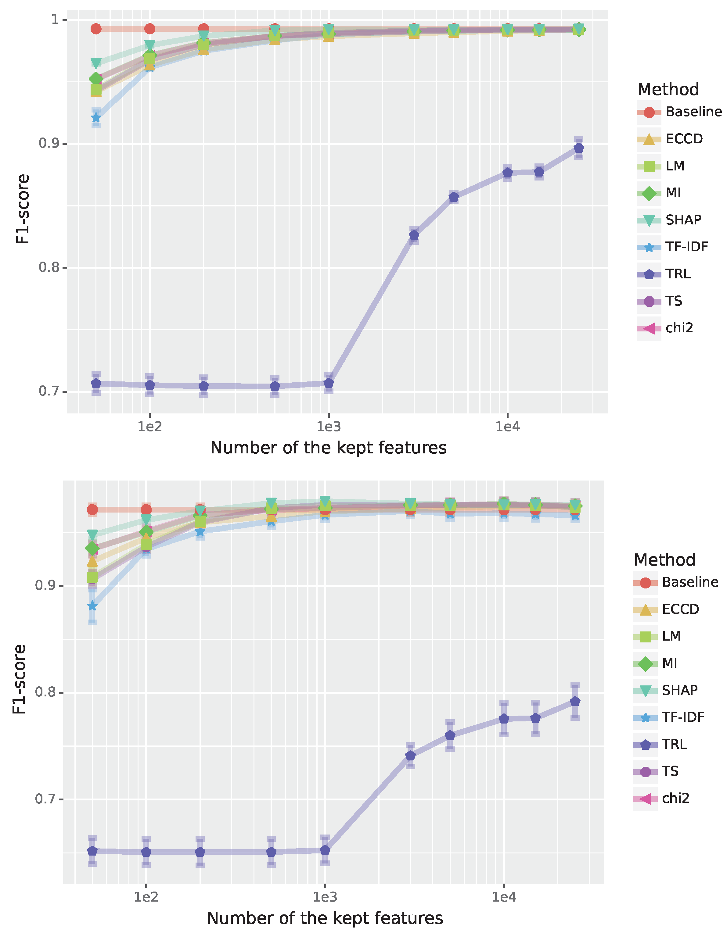
Figure 2.
Performance for the Brown corpus genre categorization (multi-class classification). The F1-scores are shown in dependence on the number of features; see legend for the color code of the feature selection method. Top: Results for training data. Bottom: Results for test data.
Figure 2.
Performance for the Brown corpus genre categorization (multi-class classification). The F1-scores are shown in dependence on the number of features; see legend for the color code of the feature selection method. Top: Results for training data. Bottom: Results for test data.
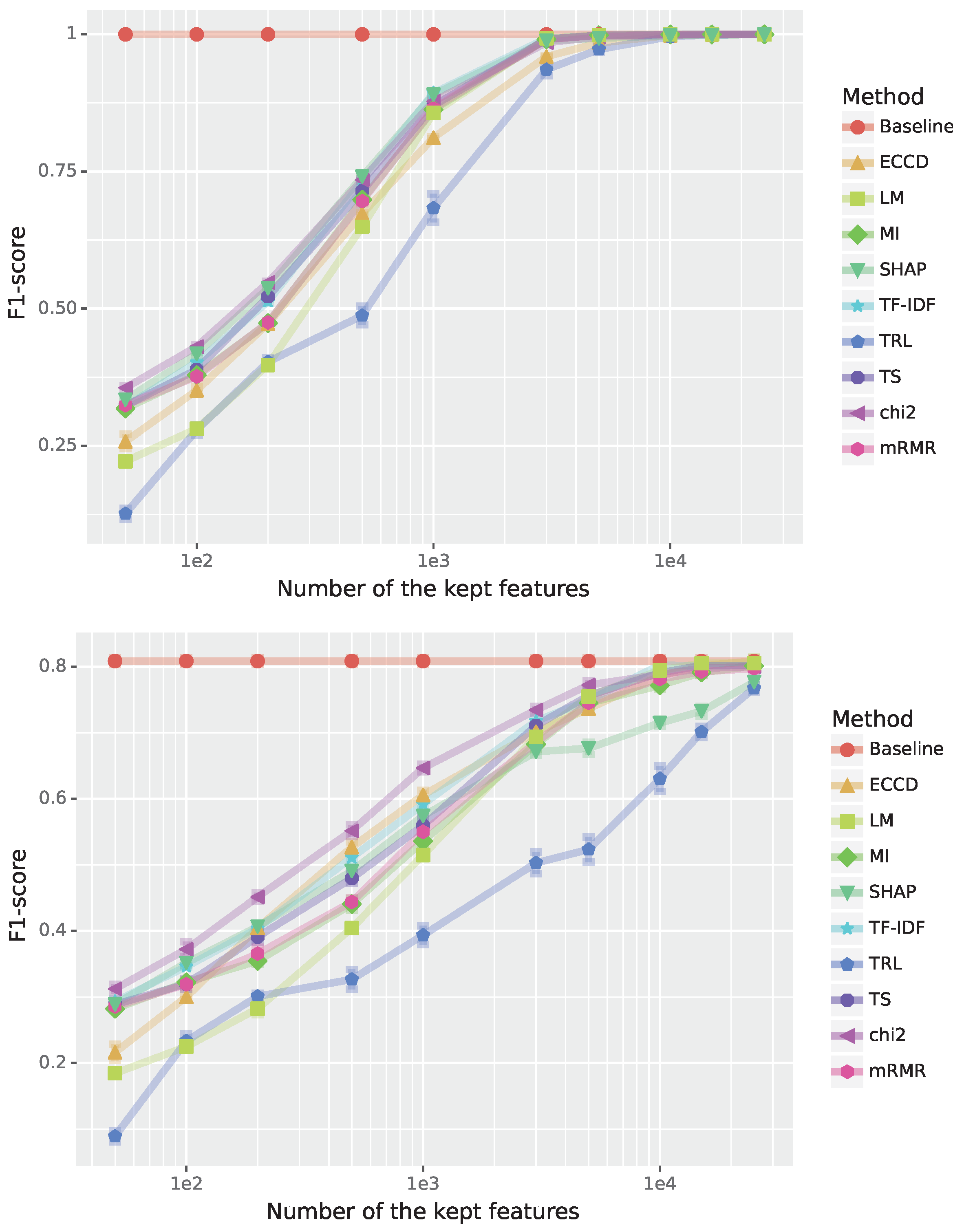
Figure 3.
Performance for the Brown corpus genre categorization (multi-class classification). The F1-scores are shown in dependence on the number of removed (best) features; see legend for the color code of the feature selection method. Top: Results for training data. Bottom: Results for test data.
Figure 3.
Performance for the Brown corpus genre categorization (multi-class classification). The F1-scores are shown in dependence on the number of removed (best) features; see legend for the color code of the feature selection method. Top: Results for training data. Bottom: Results for test data.

Figure 4.
Performance for the Arcene cancer classification (binary classification). The F1-scores are shown in dependence on the number of features; see legend for the color code of the feature selection method. Top: Results for training data. Bottom: Results for test data.
Figure 4.
Performance for the Arcene cancer classification (binary classification). The F1-scores are shown in dependence on the number of features; see legend for the color code of the feature selection method. Top: Results for training data. Bottom: Results for test data.
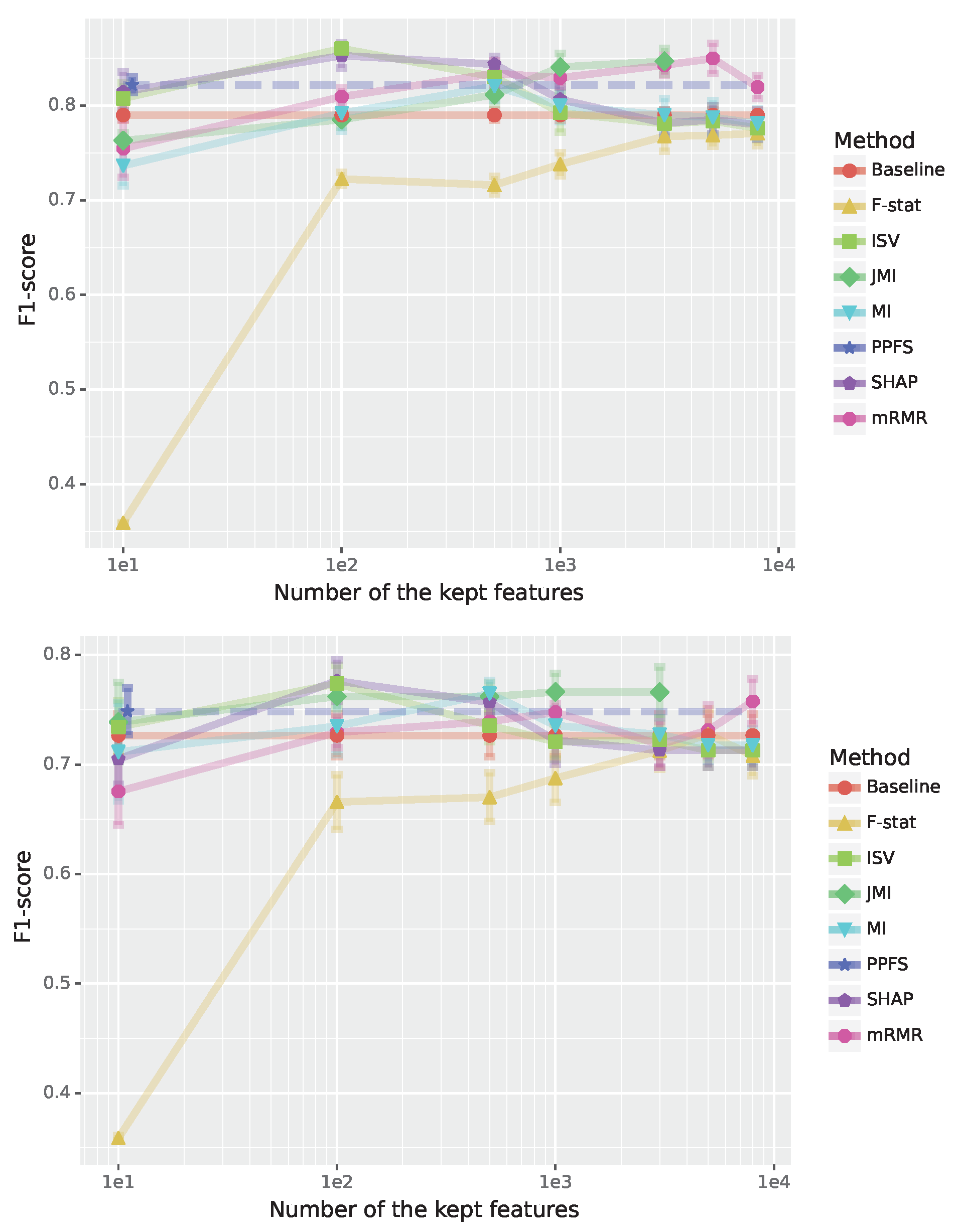
Figure 5.
Performance for the Ionosphere radar signals (binary classification). The F1-scores are shown in dependence on the number of features; see legend for the color code of the feature selection method. Top: Results for training data. Bottom: Results for test data.
Figure 5.
Performance for the Ionosphere radar signals (binary classification). The F1-scores are shown in dependence on the number of features; see legend for the color code of the feature selection method. Top: Results for training data. Bottom: Results for test data.
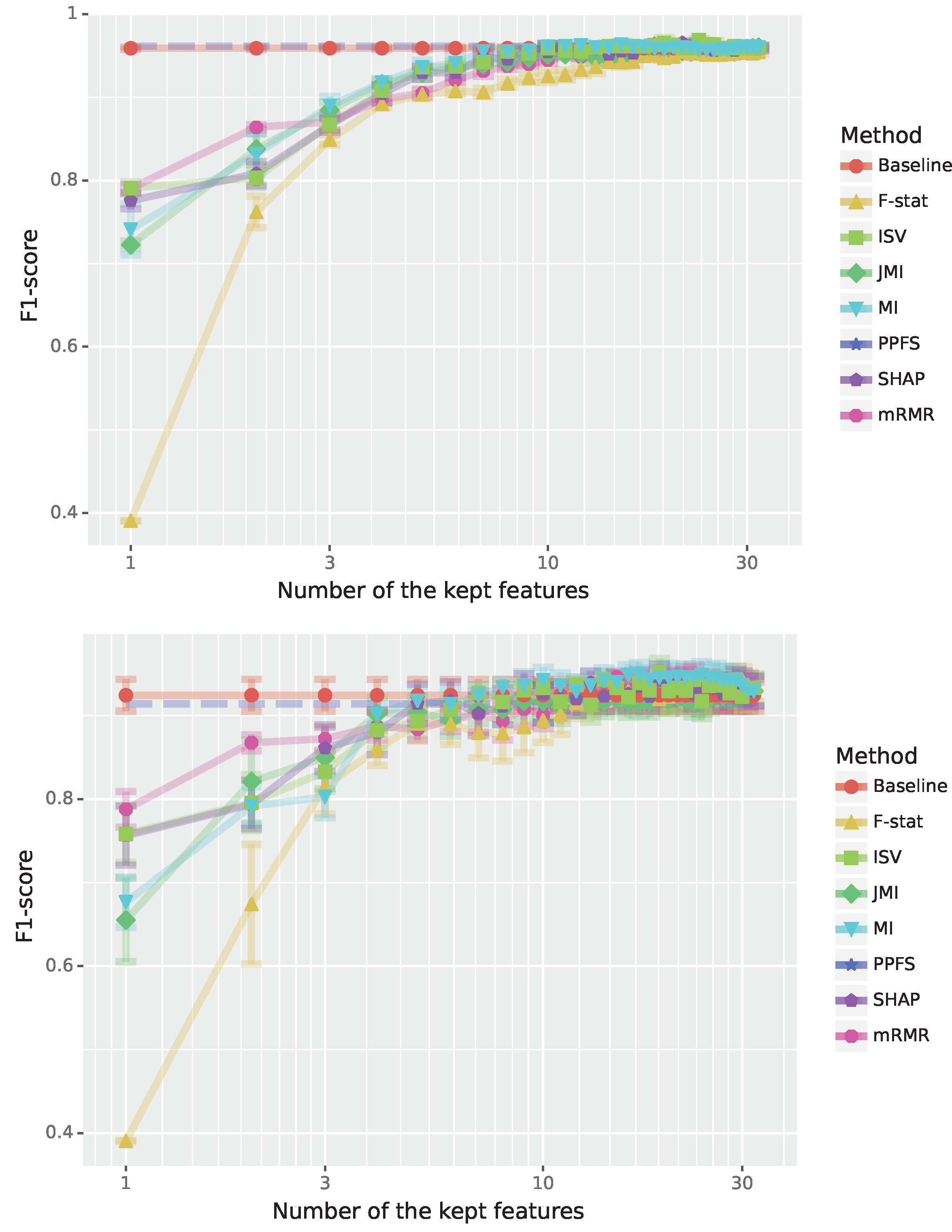
Figure 6.
Runtime of the feature methods in dependence on the number of features in a dataset.
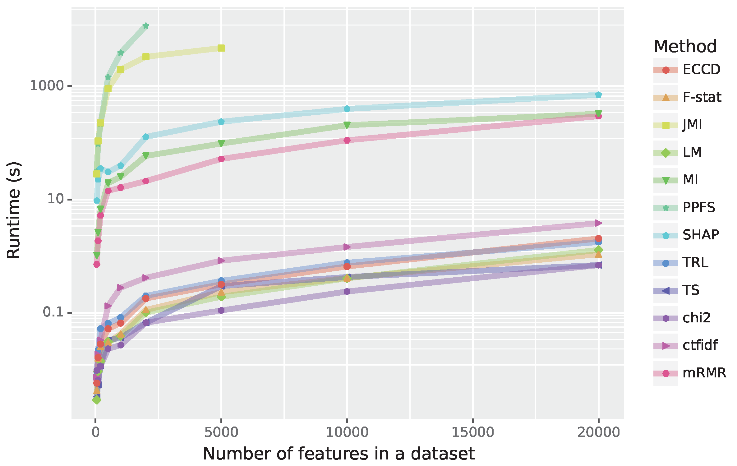
Figure 7.
Summary of all results. The best performing feature selection method over all sizes of feature sets (FS) is shown in bold. The feature selection method in bracket indicates that the best performing method performs unsatisfactorily. LFS (large feature sets), SFS (small feature sets) and VSFS (very small feature sets)
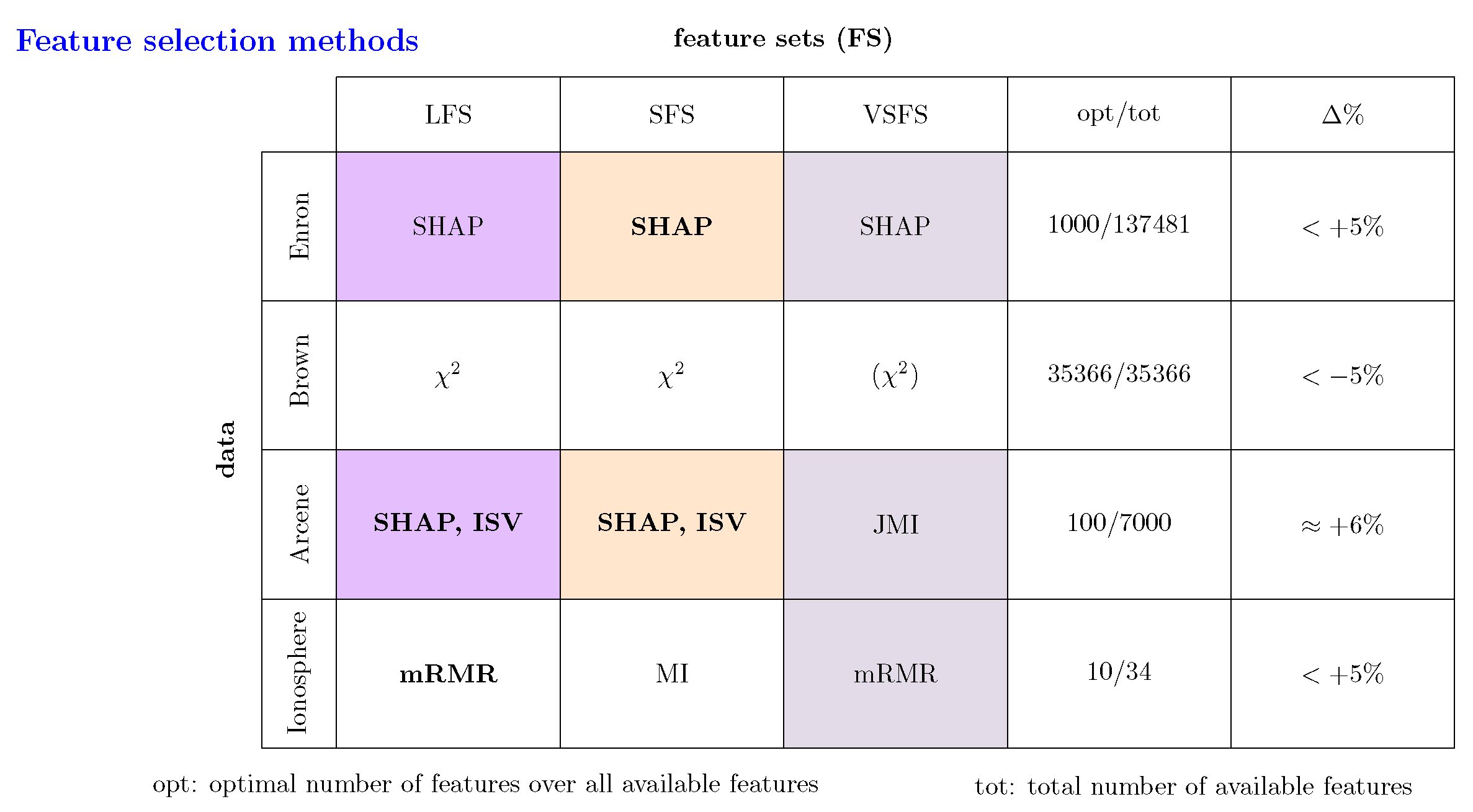

Table 1.
Jaccard scores for the Enron data. Shown are the Jaccard scores between features from the Shapley based method and all other feature selection methods for a different number of features (first column).
Table 1.
Jaccard scores for the Enron data. Shown are the Jaccard scores between features from the Shapley based method and all other feature selection methods for a different number of features (first column).
| ECCD | MI | TRL | LM | TS | TF-IDF | ||
|---|---|---|---|---|---|---|---|
| features | |||||||
| 50 | 0.205 | 0.351 | 0.075 | 0.235 | 0.220 | 0.266 | 0.299 |
| 100 | 0.235 | 0.351 | 0.047 | 0.282 | 0.266 | 0.282 | 0.351 |
| 200 | 0.286 | 0.394 | 0.042 | 0.356 | 0.338 | 0.270 | 0.375 |
| 500 | 0.247 | 0.344 | 0.018 | 0.445 | 0.422 | 0.357 | 0.350 |
| 1000 | 0.214 | 0.299 | 0.010 | 0.505 | 0.499 | 0.463 | 0.305 |
| 3000 | 0.099 | 0.132 | 0.016 | 0.192 | 0.191 | 0.184 | 0.137 |
| 5000 | 0.082 | 0.100 | 0.024 | 0.125 | 0.125 | 0.121 | 0.102 |
| 10000 | 0.070 | 0.076 | 0.042 | 0.085 | 0.085 | 0.085 | 0.077 |
| 15000 | 0.082 | 0.086 | 0.037 | 0.092 | 0.092 | 0.092 | 0.087 |
| 25000 | 0.112 | 0.113 | 0.110 | 0.113 | 0.113 | 0.114 | 0.113 |
Table 2.
Jaccard scores between all feature selection methods for the Enron data. The shown results are for 3000 features.
Table 2.
Jaccard scores between all feature selection methods for the Enron data. The shown results are for 3000 features.
| ECCD | SHAP | MI | TRL | LM | TS | TF-IDF | ||
|---|---|---|---|---|---|---|---|---|
| ECCD | 1.000 | 0.099 | 0.757 | 0.001 | 0.354 | 0.338 | 0.360 | 0.679 |
| SHAP | 0.099 | 1.000 | 0.132 | 0.016 | 0.192 | 0.191 | 0.184 | 0.137 |
| MI | 0.757 | 0.132 | 1.000 | 0.003 | 0.483 | 0.463 | 0.475 | 0.895 |
| TRL | 0.001 | 0.016 | 0.003 | 1.000 | 0.011 | 0.011 | 0.009 | 0.003 |
| LM | 0.354 | 0.192 | 0.483 | 0.011 | 1.000 | 0.963 | 0.815 | 0.519 |
| TS | 0.338 | 0.191 | 0.463 | 0.011 | 0.963 | 1.000 | 0.816 | 0.499 |
| TF-IDF | 0.360 | 0.184 | 0.475 | 0.009 | 0.815 | 0.816 | 1.000 | 0.505 |
| chi2 | 0.679 | 0.137 | 0.895 | 0.003 | 0.519 | 0.499 | 0.505 | 1.000 |
Table 3.
Jaccard score between all feature selection methods for 10000 features for the Brown data.
| TF-IDF | mRMR | TRL | LM | TS | MI | ECCD | SHAP | ||
|---|---|---|---|---|---|---|---|---|---|
| TF-IDF | 1.000 | 0.639 | 0.388 | 0.446 | 0.651 | 0.643 | 0.454 | 0.568 | 0.299 |
| mRMR | 0.639 | 1.000 | 0.451 | 0.530 | 0.743 | 0.825 | 0.387 | 0.494 | 0.309 |
| TRL | 0.388 | 0.451 | 1.000 | 0.313 | 0.433 | 0.448 | 0.210 | 0.283 | 0.281 |
| LM | 0.446 | 0.530 | 0.313 | 1.000 | 0.558 | 0.533 | 0.411 | 0.442 | 0.262 |
| TS | 0.651 | 0.743 | 0.433 | 0.558 | 1.000 | 0.745 | 0.398 | 0.548 | 0.304 |
| MI | 0.643 | 0.825 | 0.448 | 0.533 | 0.745 | 1.000 | 0.388 | 0.500 | 0.306 |
| ECCD | 0.454 | 0.387 | 0.210 | 0.411 | 0.398 | 0.388 | 1.000 | 0.550 | 0.223 |
| 0.568 | 0.494 | 0.283 | 0.442 | 0.548 | 0.500 | 0.550 | 1.000 | 0.269 | |
| SHAP | 0.299 | 0.309 | 0.281 | 0.262 | 0.304 | 0.306 | 0.223 | 0.269 | 1.000 |
Table 4.
Results for the Arcene data. Jaccard score between all feature selection methods for 100 features.
Table 4.
Results for the Arcene data. Jaccard score between all feature selection methods for 100 features.
| F-stat | MI | ISV | mRMR | JMI | SHAP | |
|---|---|---|---|---|---|---|
| F-stat | 1.000 | 0.015 | 0.010 | 0.010 | 0.005 | 0.010 |
| MI | 0.015 | 1.000 | 0.026 | 0.020 | 0.015 | 0.031 |
| ISV | 0.010 | 0.026 | 1.000 | 0.036 | 0.005 | 0.099 |
| mRMR | 0.010 | 0.020 | 0.036 | 1.000 | 0.010 | 0.026 |
| JMI | 0.005 | 0.015 | 0.005 | 0.010 | 1.000 | 0.005 |
| SHAP | 0.010 | 0.031 | 0.099 | 0.026 | 0.005 | 1.000 |
Table 5.
Results for the the Ionosphere dataset. Jaccard score between all feature selection methods for 5 features.
Table 5.
Results for the the Ionosphere dataset. Jaccard score between all feature selection methods for 5 features.
| SHAP | JMI | ISV | MI | mRMR | F-stat | |
|---|---|---|---|---|---|---|
| SHAP | 1.000 | 0.250 | 0.429 | 0.250 | 0.111 | 0.250 |
| JMI | 0.250 | 1.000 | 0.250 | 0.250 | 0.250 | 0.111 |
| ISV | 0.429 | 0.250 | 1.000 | 0.429 | 0.111 | 0.250 |
| MI | 0.250 | 0.250 | 0.429 | 1.000 | 0.111 | 0.429 |
| mRMR | 0.111 | 0.250 | 0.111 | 0.111 | 1.000 | 0.429 |
| F-stat | 0.250 | 0.111 | 0.250 | 0.429 | 0.429 | 1.000 |
Table 6.
Time complexity of the different feature selection methods.
| Method | Time Complexity | Notes |
|---|---|---|
| c-TFIDF | n: number of features, L: average length of all documents in a class. | |
| JMI | n: number of features, d: number of samples | |
| TS | n: number of features, d: number of samples | |
| MI | with optimization is possible | |
| with optimization is possible | ||
| TRL | m: number of classes, n: number of features, d: samples | |
| ECCD | m: number of classes, n: number of features, d: samples | |
| LM | m: number of classes, n: number of features, d: samples | |
| F-stat | n: number of features, d: number of samples | |
| SHAP | d: max depth of a tree model, t: number of trees in a model, l: maximum number of leaves | |
| LFS | n: all features, k: number of selected features | |
| SFS | n: number of features | |
| PPFS | b: copies, k: folds, n: features | |
| mRMR | n: features, d: samples | |
| ISV | n: all features, k: number of selected features |
Disclaimer/Publisher’s Note: The statements, opinions and data contained in all publications are solely those of the individual author(s) and contributor(s) and not of MDPI and/or the editor(s). MDPI and/or the editor(s) disclaim responsibility for any injury to people or property resulting from any ideas, methods, instructions or products referred to in the content. |
© 2025 by the authors. Licensee MDPI, Basel, Switzerland. This article is an open access article distributed under the terms and conditions of the Creative Commons Attribution (CC BY) license (http://creativecommons.org/licenses/by/4.0/).
Copyright: This open access article is published under a Creative Commons CC BY 4.0 license, which permit the free download, distribution, and reuse, provided that the author and preprint are cited in any reuse.


