Analysis of Resampling Methods for the Red Edge Band of MSI/Sentinel-2 for Coffee Cultivation Monitoring

Rozymario Bittencourt Fagundes; Édson L. Bolfe; Manuela Ramos-Ospina

doi:10.20944/preprints202502.1493.v1

Submitted:

18 February 2025

Posted:

19 February 2025

Read the latest preprint version here

Abstract

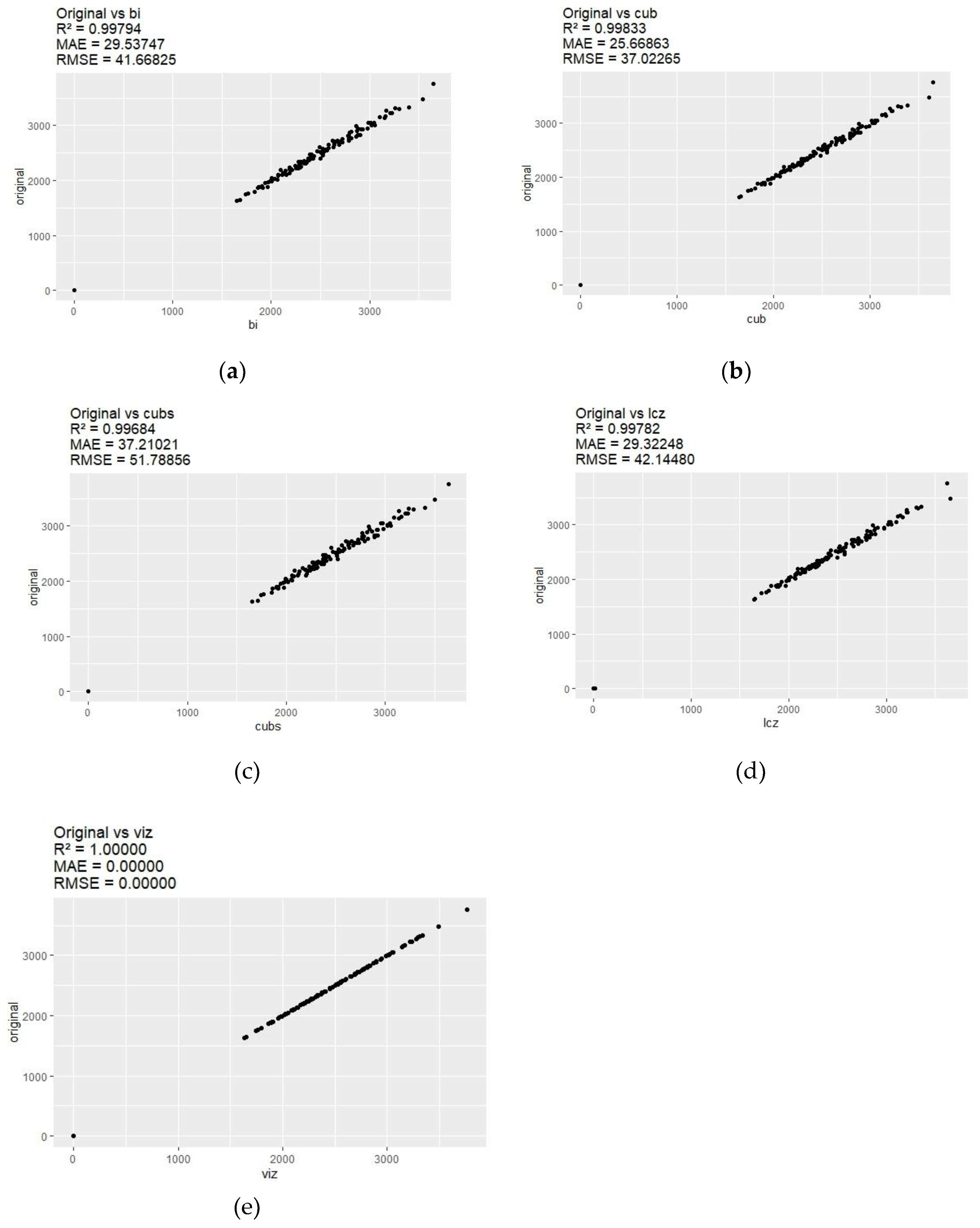
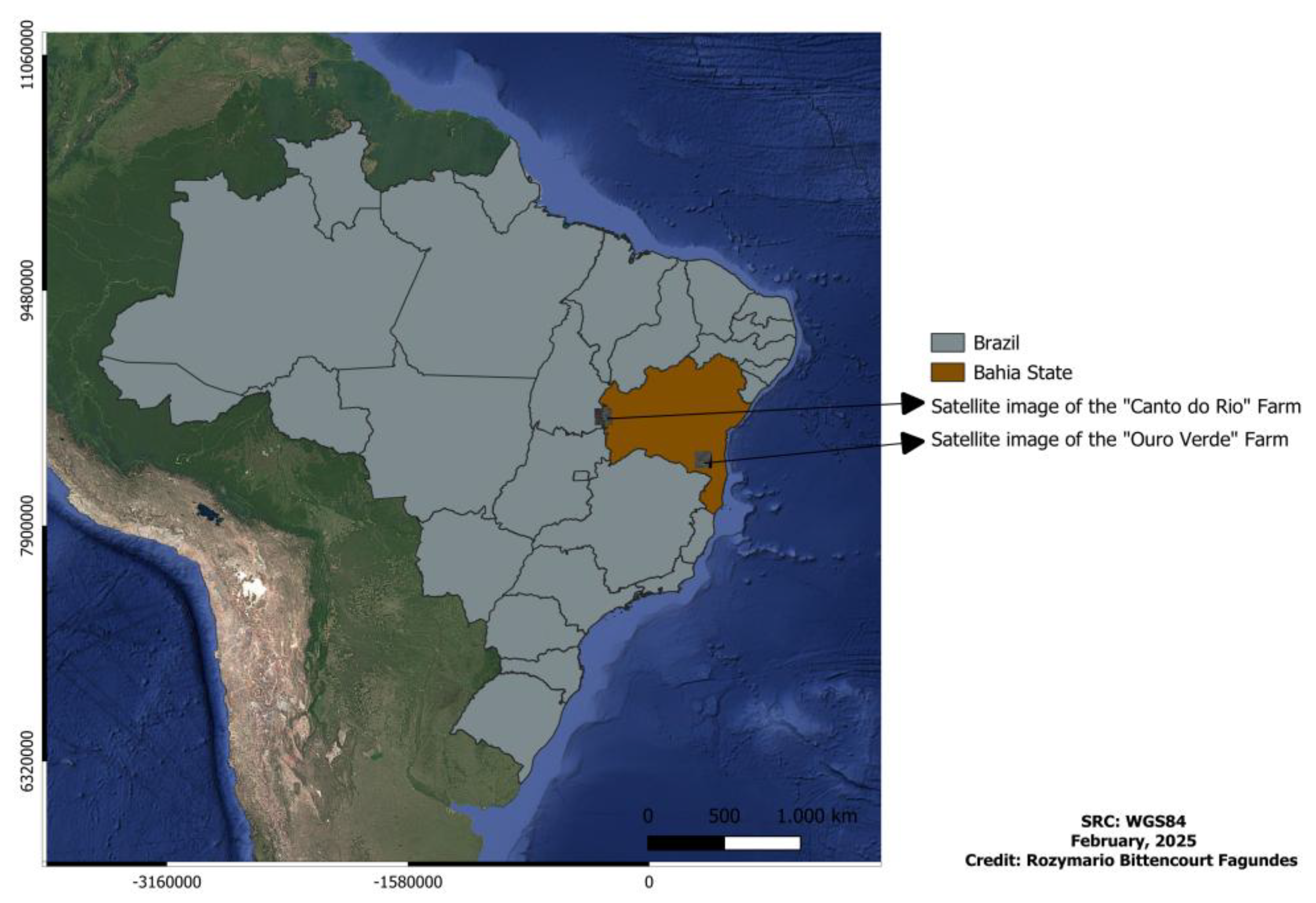
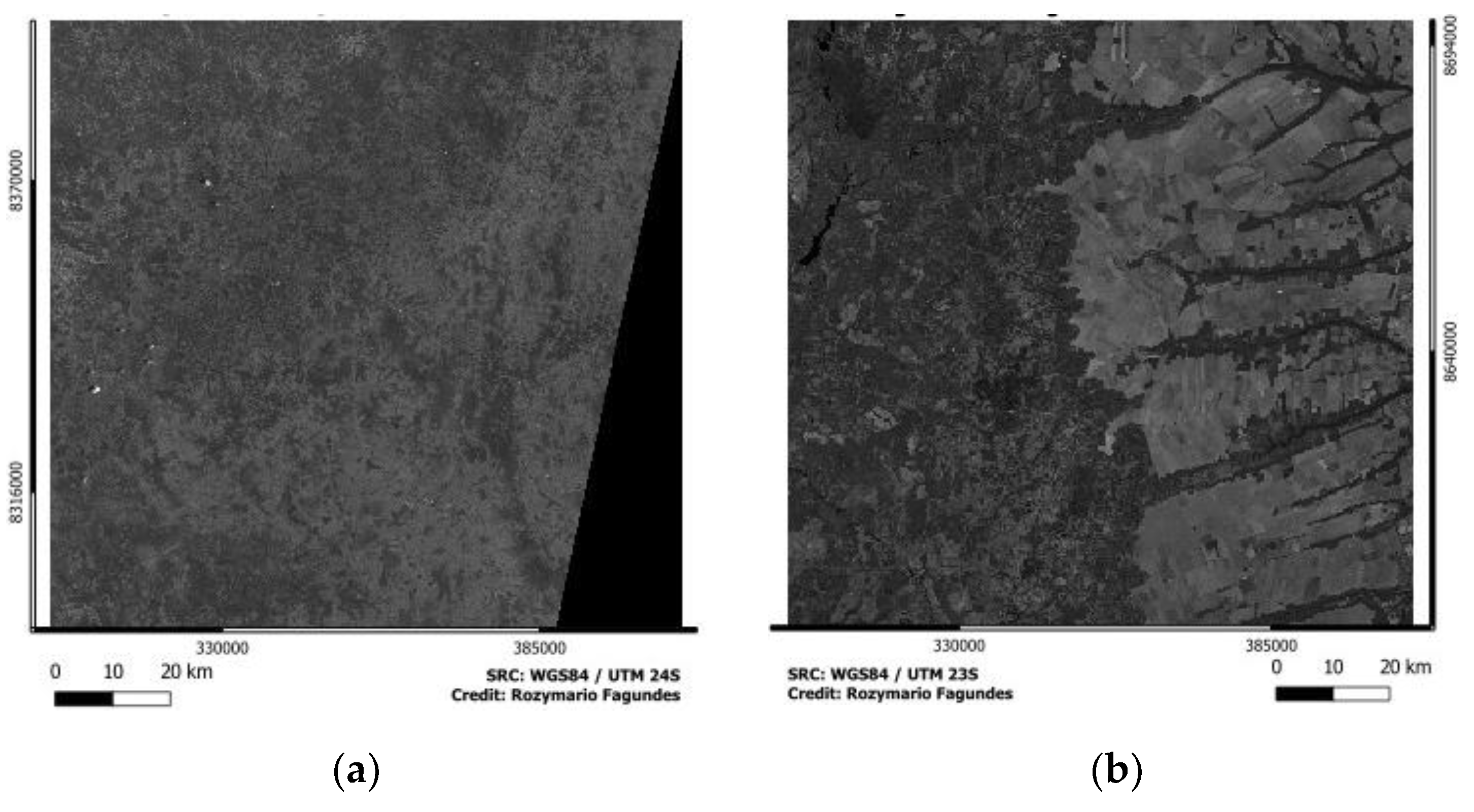
Spectral indices such as NDRE (Normalized Difference Red Edge Index), CCCI (Canopy Chlorophyll Content Index), and IRECI (Inverted Red Edge Chlorophyll Index), based on the Red Edge band of MSI/Sentinel-2 (B05, B06, B07 images), are essential tools in coffee monitoring. These indices require resampling the Red Edge band (20 m resolution) to match the NIR (10 m resolution) using methods such as nearest neighbor, bilinear, cubic, and Lanczos. In this technical note, we evaluated these resampling methods using two original B05 images, selected on November 24, 2023, and September 21, 2023, with reference points from the farms "Ouro Verde" (15 hectares) in Barra do Choça (BA) and "Canto do Rio" (45 hectares) in Luís Eduardo Magalhães (BA), respectively. A total of 500 random points were generated and analyzed using PSF, linear models, and cross-validation with metrics such as R², MAE, and RMSE. The PSF analysis indicated the integrity of the data for further analysis. The cubic method showed the best performance (R² = 0.996, MAE = 20.87, RMSE = 32.67). The validation results of the resampling methods suggest that this procedure is crucial for accurate digital processing in remote sensing for coffee cultivation and should be aligned with the study objectives.

Keywords:

remote sensing

;

precision coffee growing

;

spectral indices

Subject:

Environmental and Earth Sciences - Remote Sensing

1. Introduction

Studies on orbital remote sensing in coffee production have advanced in several countries, contributing to the improvement of production area management and increasing competitiveness in the global market [1,2].

This is especially important for Brazil, as the country is the world's largest producer and exporter of coffee beans, with 54.76 million 60-kilogram bags produced in 2024. In total, there are more than 330,000 coffee producers, 78% of whom are small-scale farmers, spread across approximately 1,900 municipalities [24,25].

These advancements are due to the introduction of Precision Agriculture (PA), which refers to the use of geotechnologies for efficient, profitable, and sustainable rural management. When applied to coffee production, PA is referred to as Precision Coffee Farming (PCF) [3,4].

Among these geotechnologies is orbital Remote Sensing (RS), conducted using satellite imagery. The applications of this technology range from identifying zones of productive potential and management areas, mapping and classifying areas, crop forecasting, and productivity estimation, to identifying diseases and pests, verifying leaf nitrogen content, and analyzing the spatial variability of crop attributes [5,6].

Several spectral indices are used in the remote monitoring of coffee farming, particularly those that include the Red Edge spectral band in their composition, such as the NDRE (Normalized Difference Red Edge Index), the CCCI (Canopy Chlorophyll Content Index), and the IRECI (Inverted Red Edge Chlorophyll Index). These indices have demonstrated strong correlations with leaf nitrogen content and productivity forecasting [7,8].

One of the main methods for obtaining these indices is through the MSI (Multispectral Instrument) Sentinel-2 sensor [9], which features 13 spectral bands, three of which are within the Red Edge range, at wavelengths of 705 nm (B05), 740 nm (B06), and 783 nm (B07). All three have a spatial resolution of 20 meters, as shown in Table 1.

To calculate the indices mentioned above, combinations are made with other spectral bands of different spatial resolutions, such as the NIR band, which has 10-meter resolution. This requires resampling the Red Edge band to a 10-meter resolution during digital processing.

Resampling involves transforming the pixel size of the original image, correcting reference points, or adjusting spatial resolution using various interpolation methods [10,11,12,13,14,15,16,17,18,19,20,21,22,23,24,25,26], such as nearest neighbor, bilinear, cubic, and Lanczos, as described in Table 2.

Based on the description of the methods, it is hypothesized that the nearest neighbor model might achieve good results, not because it is the most suitable model, but due to its characteristic of preserving the original image data.

This characteristic, however, can be misleading and not suitable for orbital remote sensing of coffee farming. Perhaps for this reason, researchers have opted for the bilinear method, with resampling of the B05 band from 20 to 10 meters of spatial resolution, as seen in a study on the effect of hailstorms on Arabica coffee crops using NDVI and NDRE indices [11].

This study employed the Semi-Automatic Classification (SPC) plugin in QGIS and concluded that NDRE is more sensitive than NDVI in demonstrating variations in vegetation index values across different Arabica coffee varieties. The same procedure was followed by other researchers [12].

Although the effects of these methods are well documented in the literature, they have been overlooked in studies on remote sensing of coffee farming that utilize the Red Edge spectral band from the MSI/Sentinel-2, as well as in the validation of these methods, depending on the specific objectives of the resampling.

On the other hand, research on the topic has been conducted, including reviews of resampling methods applied to different types of images and their forms of quantitative and qualitative validation, both in hyperspectral and multispectral images, as is the case with the MSI/Sentinel-2 sensor [13].

In this context, this technical note aims to test and validate different resampling methods for the Red Edge spectral band of the MSI/Sentinel-2, with the objective of obtaining indices for monitoring coffee farming and enhancing digital processing for this purpose.

2. Materials and Methods

Two images of the B05 band from the MSI/Sentinel-2 (L2A) were acquired, corresponding to two Arabica coffee (Coffea arabica L.) production areas in the state of Bahia, Brazil, both with 0% cloud cover.

The reference areas are the “Ouro Verde” farm, located in Barra do Choça (15 ha), in the Southwest region, and the “Canto do Rio” farm, in Luís Eduardo Magalhães (45 ha), in the Western region, dated November 24, 2023, and September 21, 2023, respectively. Details of the original images in Figure 1.

Initially, 500 random points were generated from the original image (B05), as shown in Figure 1. The values were extracted, and Spatial Point Pattern Analysis (PSF) was performed to measure spatial patterns and identify clustering or dispersion at different scales (Ripley's K Function), the distribution of the distance between nearest points (G Function), and the distribution of the distances of points to others in the set (F Function) (14-15).

For digital resampling processing, the R package terra (version 4.4.0) was used, employing the nearest neighbor, bilinear, cubic, cubic spline, and Lanczos methods to resample the B05 images from 20 to 10 meters of spatial resolution.

Next, cross-validation testing was performed, with data split into 70% training and 30% testing, and evaluation carried out through the calculation of the Coefficient of Determination (R²), Mean Absolute Error (MAE), and Root Mean Square Error (RMSE) [16,17]. All digital processing, testing, and evaluation were conducted in R.

3. Results

After resampling in R, all output images had a 10-meter spatial resolution, according to the methods used. Then, it followed for the evaluation of the sample points.

3.1. Results of the Family Health Program (FHP) Evaluation

3.1.1.“. Ouro Verde” Farm

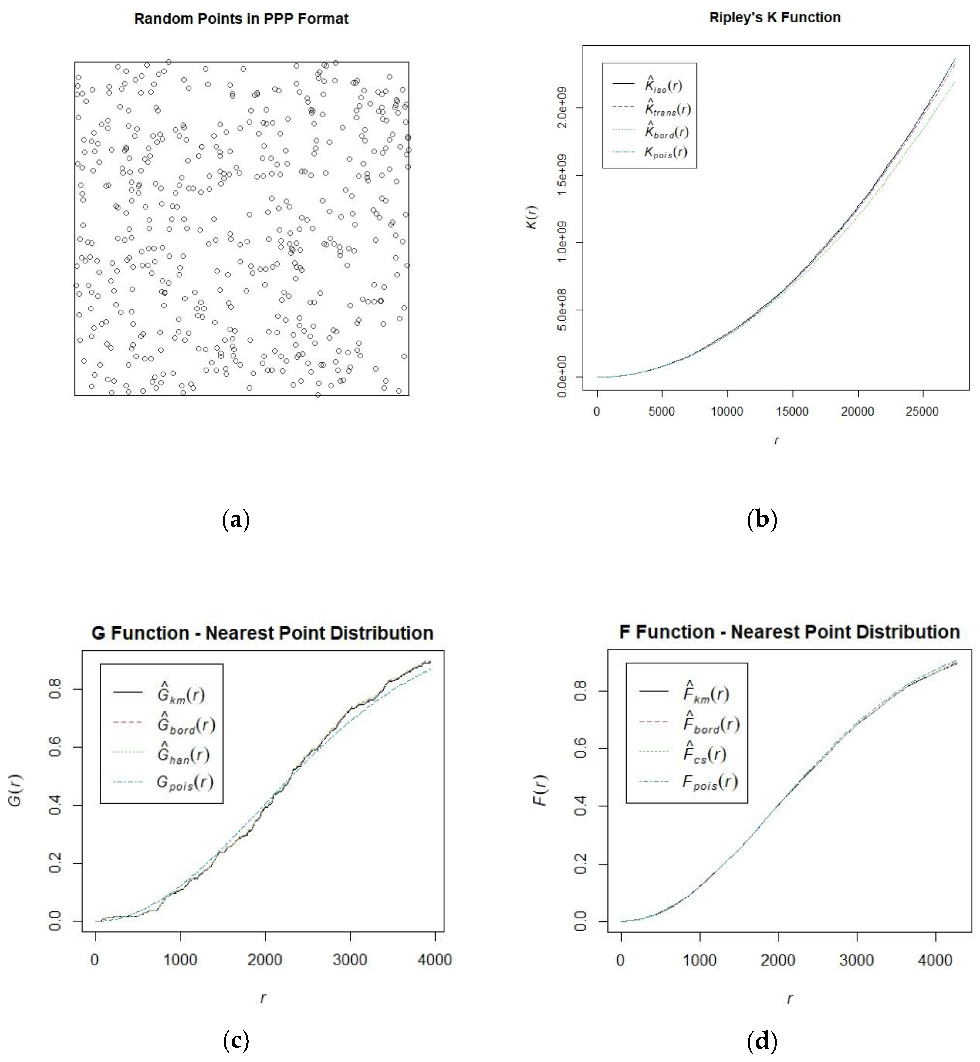
Figure 2. a) Random sample points; b) Ripley's K Function; c) G Function; d) F Function.

Table 3. Results Ripley’s K Function.

	r	theo	border	trans	iso
Min.	0	0.000e+00	0.000e+00	0.000e+00	0.000e+00
1st Qu	6862	1,48E+11	1,47E+11	1,46E+11	1,46E+11
Median	13725	5,92E+11	6,01E+11	6,00E+11	5,98E+11
Mean	13725	7,90E+11	7,86E+11	7,90E+11	7,87E+11
3rd Qu	20588	1,33E+12	1,33E+12	1,33E+12	1,32E+12
Max	27450	2,37E+12	2,33E+12	2,37E+12	2,36E+12

In the Ripley's K function, the density of points is measured as a function of distance r, with an assessment of clustering or dispersion. According to the data, the distance ranges from 0 to 27,450 units, characterizing a wide scale that allows the identification of patterns at short and long distances.

Theoretically, density increases with distance indicating a random pattern. The mean values (border, trans, iso), in turn, vary between 7.86e+11 and 7.90e+11, and are above the expected values at some scales. Regarding clustering, the maximum observed density was 2.33e+09 to 2.37e+09, suggesting strong clustering at larger scales.

The results were consistent, with close values indicating that they are reliable. There is a tendency for points to cluster at larger scales (r>20,000) and behave close to random at smaller scales.

Table 4. Results G Function.

	r	theo	han	rs	km	hazard	theohaz
Min.	0	0.0000	0.0000	0.0000	0.0000	0.0000000	0.0000000
1st Qu	2350	0.5130	0.5175	0.5131	0.5134	0.0000000	0.0006124
Median	4700	0.9438	0.9353	0.9357	0.9300	0.0000000	0.0012248
Mean	4700	0.7383	0.7290	0.7278	0.7267	0.0006211	0.0012248
3rd Qu	7050	0.9985	10.000	10.000	10.000	0.0004483	0.0018371
Max	9400	10.000	10.000	10.000	10.000	0.0377538	0.0024495

In the G Function, we observe the proximity between points, with a highlight on local clusters. Theoretically, it should grow linearly, representing the expectation for a random pattern.

The data shows that short distances r vary from 0 to 9,400, and that the means (~0.73) and medians (~0.93) are slightly below the theoretical value, indicating proximity between points at small scales (han, rs, km).

The mean value in hazard is almost 0, suggesting the absence of significant gaps. And in the distribution, the median of 0.93 close to the theoretical value (0.94) points to a tendency of slight or subtle local clustering at small scales.

Table 5. Results F Function.

	r	theo	cs	Rs	km	hazard	theohaz
Min.	0	0.0000	0.0000	0.0000	0.0000	0.0000000	0.0000000
1st Qu	2359	0.5157	0.5254	0.5244	0.5226	0.0003114	0.0006147
Median	4718	0.9450	0.9542	0.9548	0.9541	0.0009524	0.0012294
Mean	4718	0.7345	0.7387	0.7390	0.7382	0.0009808	0.0012294
3rd Qu	7077	0.9985	0.9977	0.9978	0.9978	0.0012554	0.0018441
Max	9436	10.000	10.000	10.000	10.000	0.0064643	0.0024588

Through the F Function, we can measure the distribution of the nearest points in the total space and verify if there is uniformity or dispersion. Regarding the values of (r), there is a variation between 0 and 9,436.

A linear growth can be observed, indicating uniformity. The mean values (cs, rs, km) at ~0.73 suggest a uniform distribution with denser local areas. In hazard, the mean value of almost 0 indicates the absence of large empty areas.

In the distribution, the median of ~0.95 shows that the points are close to uniformity, but with variable local density, it is possible to deduce that the points are distributed uniformly on a large scale, with dense local areas.

3.1.2.“. Canto do Rio” Farm

The results of the PSF evaluation of the Canto do Rio Farm were similar:

Figure 3. a) Random sample points; b) Ripley’s K Function; c) G Function; d) F Function.

Table 6. Results Ripley’s K Function.

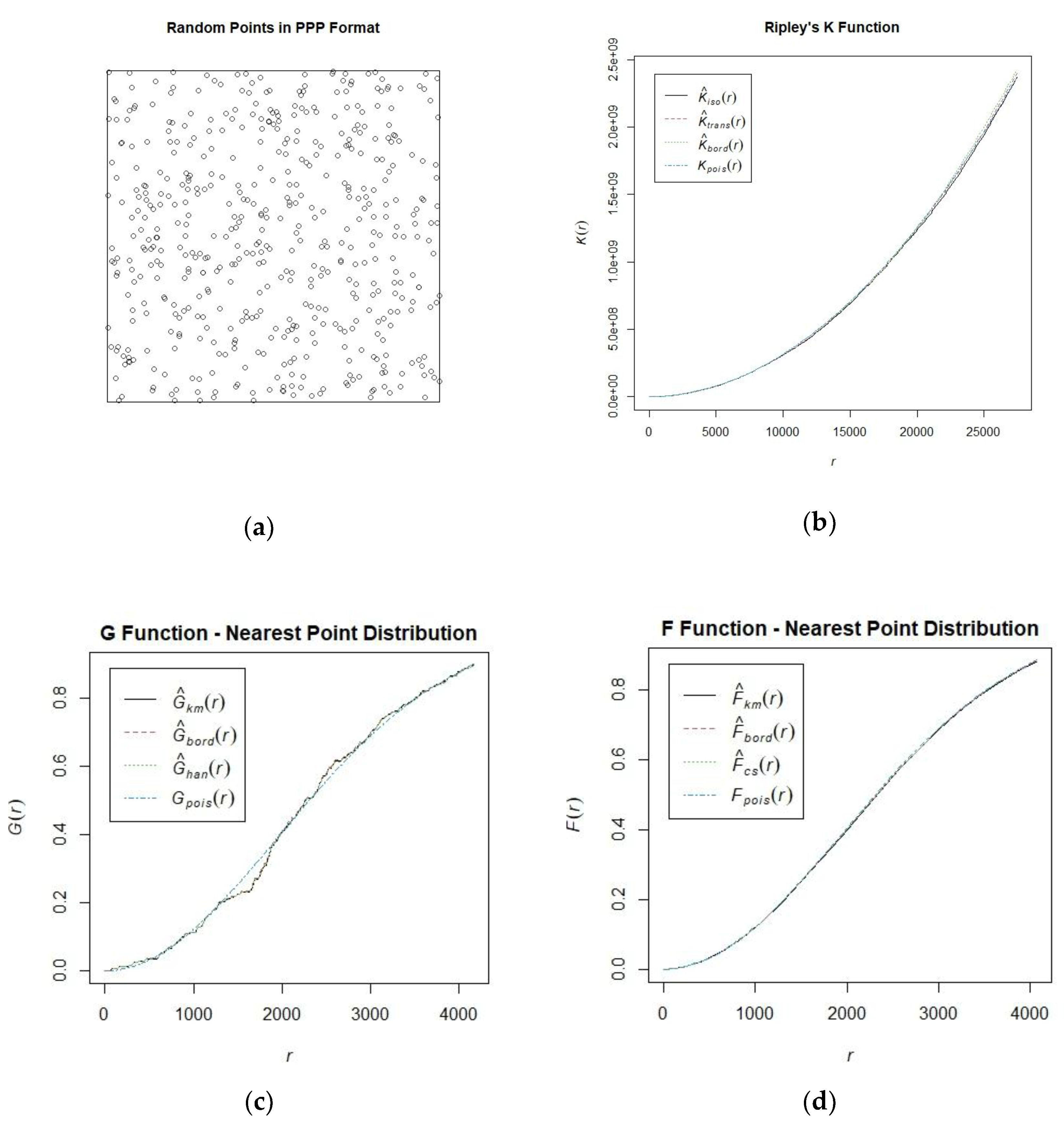
	R	theo	border	trans	iso
Min.	0	0.000e+00	0.000e+00	0.000e+00	0.000e+00
1^st Qu	6862	1,48E+11	1,47E+11	1,48E+11	1,48E+11
Median	13725	5,92E+11	5,92E+11	5,88E+11	5,85E+11
Mean	13725	7,90E+11	7,90E+11	7,89E+11	7,83E+11
3^rd Qu	20588	1,33E+12	1,33E+12	1,33E+12	1,32E+12
Max	27450	2,37E+12	2,36E+12	2,38E+12	2,37E+12

The values of r range from 0 to 27,450 units, suggesting a wide spatial scale. In the observed average density (border, trans, iso), there is proximity to the theoretical density, but with some deviations, which may indicate slight clustering or dispersion tendencies at specific scales.

The maximum observed density (2.4e+09) exceeds the theoretical (2.3e+09), indicating clustering at larger scales. Thus, it is possible to infer that the border, trans, and iso methods present similar values and consistent results. The points show tendencies of slight clustering at larger scales (r>20,000), but close to the random pattern at smaller scales.

Table 7. Results G Function.

	R	theo	han	rs	km	hazard	theohaz
Min.	0	0.0000	0.0000	0.0000	0.0000	0.0000000	0.0000000
1^st Qu	2350	0.5130	0.5088	0.5000	0.5003	0.0000000	0.0006124
Median	4700	0.9438	0.9451	0.9447	0.9412	0.0000000	0.0012248
Mean	4700	0.7383	0.7382	0.7368	0.7355	0.0006246	0.0012248
3^rd Qu	7050	0.9985	10.000	10.000	10.000	0.0004799	0.0018371
Max	9400	10.000	10.000	10.000	10.000	0.0377538	0.0024495

In the analysis of short distances, the values of r vary from 0 to 9,400 units. The theoretical function increases linearly up to 1.0, which represents a random pattern. The average values of 0.73 in han, rs, and km are slightly below the expected, indicating greater proximity between points at smaller scales.

The average value (hazard) is almost zero, suggesting the absence of significant gaps between points. Regarding the median, the observed (0.94) is close to the theoretical (0.94), indicating a strong clustering of points, with slight proximity between short distances. There is a slight tendency of proximity at small scales, without forming highly dense patterns.

Table 8. Results F Function.

	R	theo	cs	rs	km	hazard	theohaz
Min.	0	0.0000	0.0000	0.0000	0.0000	0.000e+00	0.0000000
1^st Qu	2359	0.5157	0.5224	0.5197	0.5180	2,25E-02	0.0006147
Median	4718	0.9450	0.9496	0.9469	0.9461	6,14E-01	0.0012294
Mean	4718	0.7345	0.7363	0.7353	0.7344	8,43E-01	0.0012294
3^rd Qu	7077	0.9985	0.9998	0.9997	0.9994	1,15E+00	0.0018441
Max	9436	10.000	10.000	10.000	0.9997	3,78E+00	0.0024588

The results of the F Function show a variation of r between 0 and 9,436 units. While the theoretical function grows up to 1.0, the observed (cs, rs, km) shows that average values (0.73) are slightly below the expected, with a more dispersed pattern in some areas.

Hazard values (minimum of 0.00078) and maximum (0.0032) indicate that there are few significant empty areas. In the distribution, it is observed that the median (0.94) is almost identical to the theoretical (0.94).

The points are relatively uniform, but there are locally denser areas. In this context, it is possible to observe that the results of the two points samples follow similar patterns, with slight local clustering at G scales, strong clustering at larger stakes (K), and overall uniformity at F. The main difference between the two samples is at G, which is more evident in the Ouro Verde Farm sample.

3.2. Cross-Validation Results and Metrics Evaluation

3.2.1.“. Ouro Verde” Farm

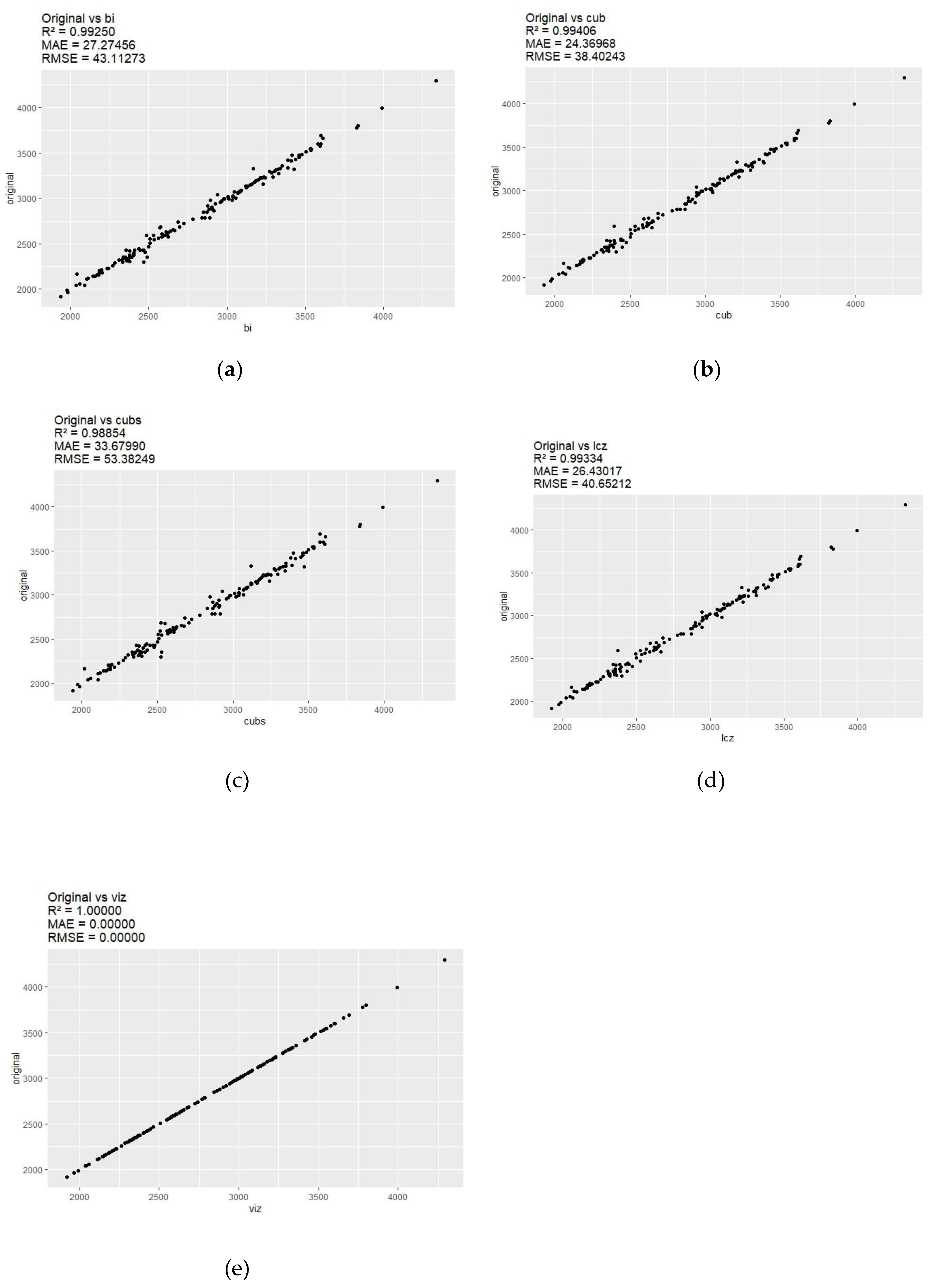
Figure 4. (a) Original image x bilinear; (b) Original image x cubic; (c) Original image x cubic spline; (d) Original image x Lanczos; (e) Original image x nearest neighbor.

3.2.1.“. Canto do Rio” Farm

Figure 5. (a) Original image x bilinear; (b) Original image x cubic; (c) Original image x cubic spline; (d) Original image x Lanczos; (e) Original image x nearest neighbor. .

The results of the cross-validation test and metric evaluation, with R² = 1, MAE = 0, and RMSE = 0 for both images, confirm the hypothesis regarding the nearest neighbor resampling method.

The other results were very close, with a slight superiority of the cubic method for both images (R² = 0.998, MAE = 35.66, RMSE = 27.02 for the Ouro Verde Farm; and R² = 0.994, MAE = 24.36, RMSE = 38.40 for the Canto do Rio Farm), followed by the bilinear methods (R² = 0.997, MAE = 29.53, RMSE = 41.66 for the Ouro Verde Farm; and R² = 0.992, MAE = 27.27, RMSE = 43.11 for the Canto do Rio Farm), Lanczos (R² = 0.997, MAE = 29.32, RMSE = 42.14 for the Ouro Verde Farm; and R² = 0.993, MAE = 26.43, RMSE = 40.65 for the Canto do Rio Farm), and cubic spline (R² = 0.996, MAE = 37.21, RMSE = 51.78 for the Ouro Verde Farm; and R² = 0.988, MAE = 33.67, RMSE = 53.38 for the Canto do Rio Farm), also for both images.

4. Discussion

The analysis on the results of the resampling methods revealed only few differences among them in terms of accuracy, appearing to be generally reliable.

Similar results were found in studies examining sugarcane crop classification and discrimination using MSI/Sentinel-2 imagery [10]. However, the authors highlight that simpler methods, such as bilinear and nearest neighbor, which require less processing time, may be preferable to more complex techniques, such as cubic and Lanczos, which demand more processing time. Although advancements in cloud processing can mitigate concerns about computational intensity.

Nearest neighbor, bilinear, and cubic methods have been widely applied in satellite image processing. For instance, Boggione & Costa [18] employed such methods for interpolating RapidEye and CBERS imagery, aiming to assess changes in grayscale values. They noted that resampling alters digital values (DVs) of the pixels in the output image, which in turn influences statistical results.

Although the study did not reach a conclusion about which method is most appropriate for the proposed work, it highlighted the importance of considering DV modifications when choosing a resampling technique. Similar effects were observed in a study using the Indian Remote Sensing (IRS) satellite images [19], aimed to determine which resampling technique preserves the image quality the most, regarding mean absolute error and peak-to-noise ratio. Alterations in DVs were shown to be dependent on the original spatial resolution and specific image operations (scaling and rotation), emphasizing that resampling-induced changes are method and context-dependent.

Beyond traditional methods, resampling has been employed to generate high-resolution images from coarse-resolution satellite data. Lezine, Kyzivat and Smith [20] explored the use of generative adversarial network (GAN), comparing the results with cubic resampling, for surface water mapping. Results suggested that GAN-based resampling can achieve comparable or superior performance than cubic resampling, when high-resolution Planet CubeSat images were downscaled and subsequently resampled to their original resolution.

Resampling methods also address challenges such as spectral mixture discrimination, where multiple spectral features are captured within a single pixel. For example, in [21] a comparison of cubic convolution and nearest neighbor resampling on Landsat imagery found no statistically significant differences in the errors associated with pixel spectral response estimation, concluding that the results had no influence on using one method over another.

Another important application of resampling is upscaling imagery for various purposes. Guo et al. [22] explored the influence of spatial resolution on soil organic carbon (SOC) mapping using hyperspectral airborne imagery, upscaling the original 1-meter resolution images by means of near neighbor, bilinear interpolation, and cubic convolution. Their study found that the use of different resampling methods has minor effects on the predictions of SOC against spatial resolution degradation.

While Lanczos resampling is less frequently used, likely due to its computational complexity, Madhukar & Narendra [23] evaluated Lanczos resampling alongside nearest neighbor and sinc methods for satellite remote sensing images, based on entropy, mean relative error and execution time metrics. They showed that Lanczos with a parameter

α = 2

achieved superior results, reducing aliasing, preserving sharpness, and minimizing ringing effects. These findings highlight the potential of Lanczos as a high-quality resampling option.

In summary, while all tested resampling methods showed minor differences in accuracy for this study, the choice of method should consider the trade-offs between computational efficiency and output quality.

5. Conclusions

The resampling of the Red Edge band for calculating NDRE aimed at coffee crop mapping can be performed using the terra package in R through the nearest neighbor, bilinear, cubic, cubic spline, and Lanczos methods, as they showed minimal differences in results.

It is important to note, however, that the nearest neighbor method, by preserving the original image data, may not provide reliable data for remote sensing of coffee cultivation. In this context, and based on the results, the best method for this purpose was determined to be cubic, followed by bilinear, Lanczos, and cubic spline.

References

CASTRO, G. D. M. de .; VILELA, E. F.; FARIA, A. L. R. de .; SILVA, R. A. .; FERREIRA, W. P. M. New vegetation index for monitoring coffee rust using sentinel-2 multispectral imagery. Coffee Science - ISSN 1984-3909, [S. l.], v. 18, p. e182170, 2023. DOI: 10.25186/.v18i.2170. Disponível em: https://coffeescience.ufla.br/index.php/Coffeescience/article/view/2170. Acesso em: 10 dec. 2024. [CrossRef]
Dias, G. Riscos climáticos e produtividade do Coffea arabica L. para as principais regiões cafeeiras do Brasil: clima presente e futuro. Tese de Doutorado aprovada em 5 de abril de 2024, no Programa de Pós-graduação em Meio Ambiente e Recursos Hídricos, da Universidade Federal de Itajubá. Itajubá-MG.
SILVA, F.M.; ALVES, M.C. Cafeicultura de Precisão. Lavras: Editora UFLA, 2013.
FERRAZ, G.A.S. Cafeicultura de Precisão: Malhas amostrais para o mapeamento de atributos do solo, da planta e recomendações. 2012, 135 f. Tese (Doutorado em Engenharia Agrícola) – Programa de Pós-Graduação em Engenharia Agrícola, Universidade Federal de Lavras, Lavras, 2012.
SANTANA, L. S.; FERRAZ, G. A. e S.; SANTOS, S. A. dos.; DIAS, J. E. L. . Precision coffee growing: A review. Coffee Science -, [S. l.], v. 17, p. e172007, 2022. ISSN 1984-3909. [CrossRef]
MELOS, N.D. Uso de análise multivariada para identificação de zonas de potenciais produtivos agrícolas. 118 f. Dissertação de Mestrado do curso de Pós-Graduação em Agricultura de Precisão do Colégio Politécnico da Universidade Federal de Santa Maria, orientada pelo prof. Dr. Lúcio de Paula Amaral, aprovada em 9 de março de 2023. Santa Maria, RS.
Chemura et al. Mapping spatial variability of foliar nitrogen in coffee (Coffea arabica L.) plantations with multispectral Sentinel-2 MSI data, ISPRS Journal of Photogrammetry and Remote Sensing, Volume 138, 2018, Pages 1-11, ISSN 0924-2716.
Nogueira Martins, R.; de Carvalho Pinto, F.d.A.; Marçal de Queiroz, D.; Magalhães Valente, D.S.; Fim Rosas, J.T. A Novel Vegetation Index for Coffee Ripeness Monitoring Using Aerial Imagery. Remote Sens. 2021, 13, 263. [CrossRef]
ESA - AGÊNCIA ESPACIAL EUROPEIA. Sentinel Online. Disponível em: https://sentinels.copernicus.eu/web/sentinel/home. Acesso em: 12/12/2024.
P. M. Kai, B. M. de Oliveira, G. S. Vieira, F. Soares and R. M. Costa, "Effects of resampling image methods in sugarcane classification and the potential use of vegetation indices related to chlorophyll," 2021 IEEE 45th Annual Computers, Software, and Applications Conference (COMPSAC), Madrid, Spain, 2021, pp. 1526-1531. [CrossRef]
Rodrigues, S. A., Cortez, J. W., & Henriques, H. J. R. (2021). Efeito da chuva de granizo em variedades do café arábica por meio de índices de vegetação. Agrarian, 14(54), 433–441. [CrossRef]
Feio, S. Análise multitemporal de imagens de satélite Sentinel-2 como suporte à elegibilidade das ajudas comunitárias agrícolas. Dissertação de Mestrado. Departamento de Engenharia Geográfica, Geofísica e Energia da Faculdade de Ciências, da Universidade de Lisboa. Lisboa, PT, 2017.
Mookambiga, A., Gomathi, V. Comprehensive review on fusion techniques for spatial information enhancement in hyperspectral imagery. Multidim Syst Sign Process 27, 863–889 (2016). [CrossRef]
ANJOS, A. MAZZA, M.C.M. SANTOS, .A.C. DELFINI, L.T. Análise de padrão de distribuição espacial da araucária (Araucária angustifólia) em algumas áreas do estado do Paraná, utilizando a função K de Ripley. Scientia Florestalis, n. 66, p.38-45, dez, 2004.
LOOSMORE, N. FORD, E. Stasistical inference using the G or K point pattern spatial statistics. September 2006, Ecology 87(8):1925-31. [CrossRef]
ZANZARINI, F. V.; PISARRA, T. C. T.; BRANDÃO, F. J. C.; TEIXEIRA, D. D. B. Correlação espacial do índice de vegetação (NDVI) de imagem Landsat/ETM+ com atributos do solo. Revista Brasileira de Engenharia Agrícola e Ambiental, Campina Grande, v. 17, n. 6, p. 608-614, abril. 2013.
SPERANZA, E. A.; OLIM, G. E. de S.; INAMASU, R. Y.; VAZ, M. P.; JORGE, L. A. de C. Delineamento de zonas de manejo para o planejamento de experimento on-farm na cultura do algodão. Congresso Brasileiro de Agricultura de Precisão – ConBAP. Campinas – SP, 2022.
G. A. Boggione; D. D. Costa. REAMOSTRAGEM EM IMAGENS DE SENSORIAMENTO REMOTO: UMA ABORDAGEM SOB O PONTO DE VISTA DO MAUP. IV Simpósio Brasileiro de Geomática – SBG2017 II. Presidente Prudente - SP, 24-26 de julho de 2017 p. 315-322 ISSN 1981-6251.
Porwal, S.; Katiyar, S. K. Performance Evaluation of Various Resampling Techniques on IRS Imagery. 2014 Seventh International Conference on Contemporary Computing (IC3) 2014. [CrossRef]
Lezine, E. M. D.; Kyzivat, E. D.; Smith, L. C. Super-Resolution Surface Water Mapping on the Canadian Shield Using Planet CubeSat Images and a Generative Adversarial Network. Canadian Journal of Remote Sensing 2021, 1–15. [CrossRef]
CECCATO, G. Z.; das, N.; José Marinaldo GLERIANI; Cesar, J. AVALIAÇÃO DOS VALORES de ERRO DO MODELO LINEAR de MISTURA ESPECTRAL EM IMAGENS ETM+/LANDSAT 7 a PARTIR de REAMOSTRAGENS PELO VIZINHO MAIS PRÓXIMO E CONVOLUÇÃO CÚBICA. Geociências 2021, 40 (3), 795–810. [CrossRef]
Guo, L.; Shi, T.; Linderman, M.; Chen, Y.; Zhang, H.; Fu, P. Exploring the Influence of Spatial Resolution on the Digital Mapping of Soil Organic Carbon by Airborne Hyperspectral VNIR Imaging. Remote Sensing 2019, 11 (9), 1032–1032. [CrossRef]
Madhukar, B. N.; R. Narendra. Lanczos Resampling for the Digital Processing of Remotely Sensed Images. Lecture notes in electrical engineering 2013, 403–411. [CrossRef]
CONAB – COMPANHIA NACIONAL DE ABASTECIMENTO. Acompanhamento da safra brasileira de café, v. 11 – Safra 2024, n.4- Quarto levantamento, Brasília, p. 1-53, janeiro 2025.
CAMPO E NEGÓCIOS. Anuário de café 2021. Uberlândia, 2021.
J. A. Richards and J. Richards, Remote sensing digital image analysis. Springer, 1999, vol. 3.

Figure 1. In this figure, we see the map of Brazil, the map of the State of Bahia, and the location of the satellite images corresponding to the "Canto do Rio" and "Ouro Verde" farms.

Figure 1. These are original B05 images: a) “Ouro Verde” Farm image; b) “Canto do Rio” Farm image.

Table 1. Spectral band characteristics of MSI/Sentinel-2.

Band Number	SpectralBand	Wavelength (nm)	Spacial Resolution (m)
B01	Costal aerosol	443	60
B02	Blue	490	10
B03	Green	560	10
B04	Red	665	10
B05	Red Edge 1	705	20
B06	Red Edge 2	740	20
B07	Red Edge 3	783	20
B08	NIR	842	10
B8A	NIR narrow	865	20
B09	Water vapor	945	60
B10	Cirrus	1380	60
B11	SWIR 1	1910	60
B12	SWIR 2	2190	20

Table 2. Description of resampling methods and their effects.

Resampling Methods	Characteristics
Nearest Neighbor	Assigns the value of a pixel based on the nearest pixel, thus preserving the original image data. However, this can lead to duplication of values, loss of information, and positioning errors, requiring careful use of this method.
Bilinear	Uses the four nearest points to determine a new pixel value by applying interpolation among the pixels that intercept these points. Weighted averaging of the four closest pixels from the original image generates new output values.
Cubic	Considers the 16 nearest pixels from the original image to calculate the value of a new pixel at a specific coordinate of the resampled image. It performs weighted averaging of these points, requiring more processing time but producing smoother images due to the inclusion of more points.
Lanczos	This method preserves details and smoothens the image by using a Lanczos kernel to interpolate signal values. Although it takes more processing time, it offers better image quality.

Disclaimer/Publisher’s Note: The statements, opinions and data contained in all publications are solely those of the individual author(s) and contributor(s) and not of MDPI and/or the editor(s). MDPI and/or the editor(s) disclaim responsibility for any injury to people or property resulting from any ideas, methods, instructions or products referred to in the content.

© 2025 by the authors. Licensee MDPI, Basel, Switzerland. This article is an open access article distributed under the terms and conditions of the Creative Commons Attribution (CC BY) license (http://creativecommons.org/licenses/by/4.0/).

Copyright: This open access article is published under a Creative Commons CC BY 4.0 license, which permit the free download, distribution, and reuse, provided that the author and preprint are cited in any reuse.