Submitted:
18 February 2025
Posted:
19 February 2025
You are already at the latest version
Abstract
Variational Autoencoders (VAEs) have emerged as a promising tool for modeling volatility surfaces, with particular significance for generating synthetic implied volatility scenarios that enhance risk management capabilities. This study evaluates VAE performance using synthetic volatility surfaces, chosen specifically for their arbitrage-free properties and clean data characteristics. We demonstrate how these synthetic surfaces can serve as powerful tools for stress testing and scenario analysis, enabling risk managers to explore extreme market conditions that may not be present in historical data. Through a comparative analysis between traditional encoder-decoder reconstruction and latent space optimization methods, we explicitly test the resulting surfaces for arbitrage violations. Our results demonstrate that accurate, arbitrage-free surface reconstruction is achievable using only 5\% of the original data points, facilitating rapid generation of diverse implied volatility scenarios. This finding has important implications for market risk analysis, derivatives pricing, and the development of more robust risk management frameworks. The ability to generate synthetic yet realistic volatility surfaces enables more comprehensive stress testing, helps identify potential model vulnerabilities, and supports the validation of pricing and risk models across a wider range of market conditions than historical data alone would permit.
Keywords:
Variational Autoencoders
; Synthetic volatility
; Volatility surface
; Arbitrage
1. Introduction
Generative models are a class of statistical models that aim to learn the underlying distribution of a dataset to generate new data points that resemble the original data. These models have gained prominence due to their ability to capture complex data structures and generate realistic samples, making them invaluable in various applications, including finance.
Autoencoders have emerged as a powerful tool among the various generative models. An autoencoder is a type of neural network designed to learn efficient representations of data, typically for dimensionality reduction or feature extraction. It consists of two main components: an encoder that compresses the input data into a lower-dimensional latent space, and a decoder that reconstructs the original data from this compressed representation. This architecture allows autoencoders to learn meaningful features from the data while minimizing the reconstruction error.
Variational Autoencoders (VAEs) are a specific type of autoencoder that incorporates principles from Bayesian inference. Introduced by Kingma and Welling in 2013 [21], VAEs extend the traditional autoencoder framework by imposing a probabilistic structure on the latent space. Instead of learning a deterministic mapping from input to latent space, VAEs learn a distribution over the latent variables, allowing for the generation of new data points by sampling from this distribution. This probabilistic approach enables VAEs to capture uncertainty and variability in the data, making them particularly suitable for applications in finance, where uncertainty plays a crucial role.
The evolution of machine learning has been marked by significant milestones, from early statistical methods to the rise of deep learning. Initially, machine learning techniques were mainly focused on supervised learning tasks, where models were trained on labeled data. However, the advent of large datasets and increased computational power have facilitated the development of unsupervised and generative models. In finance, the integration of machine learning has transformed traditional approaches to risk management, asset pricing, and trading strategies. Researchers such as Fllmer, Kupiainen, and Lescourt (2016) [12] have explored the application of machine learning techniques in mathematical finance, highlighting their potential to enhance predictive accuracy and decision-making processes.
The introduction of machine learning to finance has also been supported by studies such as those of Guo et al. (2018) [18], who demonstrated the effectiveness of deep learning models in predicting stock prices, and Chataigner (2019) [5], who examined the use of generative models for option pricing. Hull and White (1990) laid the groundwork for modern option pricing models, while Broussard et al. (2020) [4] discussed the implications of machine learning in the context of volatility modeling.
Recent work has focused specifically on the application of VAE for generating implied volatility surfaces. Bergeron et al. (2021) [2] explored the use of VAEs to model and generate volatility surfaces, demonstrating their ability to capture the complex dynamics and features of these surfaces, particularly in the presence of incomplete data. Their findings indicate that VAEs can effectively fill gaps in volatility data, providing a more robust framework for volatility estimation in both liquid and illiquid markets. Furthermore, Bergeron’s work on “Hands Off Volatility" emphasizes the importance of automated and data-driven approaches to volatility modeling, advocating the use of machine learning techniques to enhance the efficiency and accuracy of volatility predictions. While Bergeron et al. pioneered VAE-based implied volatility surface generation, our research distinguishes itself by tackling the critical challenge of surface construction and completion with synthetic data. As a contribution to their approach, which primarily focuses on the generation and use of market data, we comprehensively address data sparsity through an innovative methodology that not only generates but robustly completes arbitrage-free volatility surfaces. Our key contributions include latent space optimization techniques, systematic incorporation of market features beyond traditional parameters, and the incorporation of arbitrage-free conditions in the generation of surfaces. By comparing completion via reconstruction algorithms and advanced latent space optimization.
This paper makes several significant contributions to volatility surface modeling and financial derivatives. First, we develop a robust synthetic data generation framework using parameterized Heston models, generating more than 13,500 synthetic surfaces compared to typical market availability of fewer than 100, thereby overcoming traditional barriers of limited market data. Second, we extend Bergeron et al.’s [2] latent space optimization approach, demonstrating successful reconstruction with up to 96% missing data points while maintaining essential mathematical properties. Third, we implement comprehensive arbitrage validation, preserving critical no-arbitrage conditions including calendar spread and butterfly arbitrage constraints, validated through probability distribution analysis and total variance strip non-intersection tests. Finally, we successfully integrate machine learning with financial theory, capturing complex volatility surface dynamics while maintaining mathematical properties. These advances contribute to both theoretical understanding and practical application of volatility surface modeling, particularly in markets where traditional approaches face significant data limitations.
We first define generative models in Section 2, then we provide the mathematical intuition of VAEs in Section 3. Afterward, we recall the some option pricing theory and implied volatility model in Section 4, then we develop the algorithm to generate the training dataset in Section 5. We will provide the application of perform completion by latent space optimization Section 6 and finally we give concluding remarks in Section 7.
Having established the context and goals of our research, we now turn to examine the fundamental concepts of generative modeling that underpin our methodology.
2. What Is Generative Modeling
Generative modeling is a subfield of machine learning that focuses on learning the underlying distribution of a dataset in order to generate new data points that are statistically similar to the original data. Unlike discriminative models, which aim to classify or predict outcomes based on input features, generative models seek to understand how the data is generated. This understanding allows them to create new instances that can be used for various applications, such as data augmentation, anomaly detection, and simulation.
2.1. Definition and Purpose
At its core, generative modeling involves estimating the joint probability distribution ( ) of the input data ( X ) and the corresponding labels (Y ). By learning this distribution, generative models can generate new samples ( ) that resemble the original dataset. The primary purpose of generative modeling is to capture the complex relationships and structures within the data, enabling the generation of realistic and diverse samples.
2.2. Types of Generative Models
Generative models encompass various categories, each with its unique methodology and practical applications. Gaussian Mixture Models (GMMs) are probabilistic models that assume the data is generated from a mixture of several Gaussian distributions. They are commonly used for clustering and density estimation. Hidden Markov Models (HMMs) re used for modeling sequential data, where the system is assumed to be a Markov process with hidden states, They are mostly utilized in speech recognition and bioinformatics. Generative Adversarial Networks (GANs), as introduced by Goodfellow et al. in 2014 [15], comprise two neural networks, a generator, and a discriminator, trained simultaneously.The generator creates synthetic data, while the discriminator evaluates its authenticity. This adversarial training process leads to the generation of highly realistic samples. Variational Autoencoders (VAEs), introduced by Kingma and Welling in 2013 [22], amalgamate autoencoder and variational inference principles, learning a probabilistic correlation from input data to a latent space for generating new samples. Lastly, Normalizing Flows represent a class of generative models converting a simple distribution, like Gaussian, into a more intricate form using invertible transformations to enable precise likelihood estimation and proficient sampling.
Generative models are widely used in various fields, serving multiple purposes. They can expand training datasets to enhance supervised learning models, particularly in data-scarce settings. Additionally, generative models excel at detecting anomalies by recognizing data outliers. They are instrumental in producing realistic images and videos, fostering applications in art, entertainment, and virtual reality realms. Moreover, in natural language processing, these models facilitate the generation of coherent text for chatbots, content creation automation, and language translation. Furthermore, in finance, generative models play a significant role in simulating market scenarios, generating synthetic financial data, and modeling intricate financial instruments.
While generative models provide a broad framework for data generation, we now focus specifically on Variational Autoencoders, which form the cornerstone of our approach to volatility surface modeling.
3. Mathematical Intuition of Variational Autoencoders
Variational Autoencoders (VAEs) are a powerful class of generative models that combine principles from deep learning and Bayesian inference. The mathematical intuition behind VAEs lies in their ability to learn a probabilistic representation of the data, allowing for the generation of new samples by sampling from a learned latent space. This section will provide a detailed mathematical development of the VAE model, including its formulation, loss function, and the inference process. The VAE architecture is presented in the below diagram:
Figure 1.
VAE architecture.
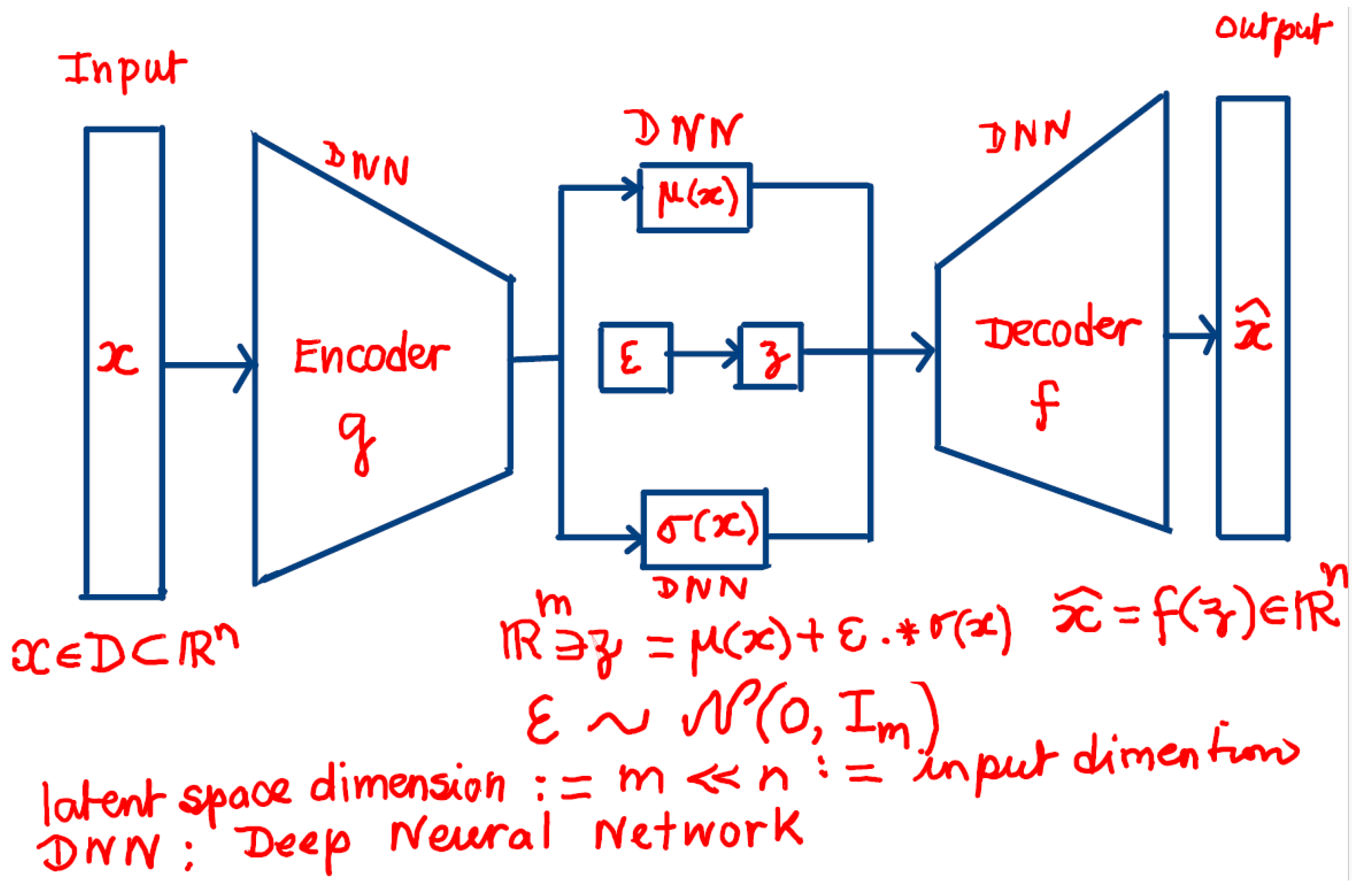
3.1. The Generative Process
In a VAE, we assume that the observed data ( ) is generated from some latent variables () through a generative process. The generative model can be expressed as:
where and ( ) are the parameters of the output distribution, typically modeled by a neural network. The latent variables ( ) are assumed to follow a prior distribution:
where () is the identity matrix, indicating that the latent variables are drawn from a standard normal distribution.
3.2. The Inference Process
The goal of a VAE is to learn the posterior distribution ( ), which is typically intractable. Instead, we approximate this posterior using a variational distribution ( ), which is also modeled by a neural network. The variational distribution is parameterized by ( ):
where ( ) and ( ) are the outputs of the encoder network.
3.3. The Evidence Lower Bound (ELBO)
To train the VAE, we maximize the marginal likelihood of the data ( ). However, since this is often intractable, we instead maximize the Evidence Lower Bound (ELBO), which can be expressed as:
where ( ) is the Kullback-Leibler divergence, measuring the difference between the variational distribution ( ) and the prior ( ).
The ELBO can be rewritten as:
The first term, , represents the expected log-likelihood of the data given the latent variables, while the second term, , acts as a regularization term that encourages the variational distribution to be close to the prior distribution.
3.4. The Loss Function
To optimize the VAE, we minimize the negative ELBO, which can be expressed as the loss function:
This loss function consists of two components:
- Reconstruction Loss: The first term measures how well the model can reconstruct the input data from the latent representation.
- Regularization Loss: The second term penalizes the divergence between the variational distribution and the prior distribution, ensuring that the learned latent space follows the desired prior distribution (standard normal distribution).
3.5. Sampling from the Latent Space
Once the VAE is trained, we can generate new samples by sampling from the prior distribution ( ) and passing the samples through the decoder network:
Sample ( ) from the prior:
Generate new data ( ) from the decoder:
This process allows the VAE to generate new data points that are consistent with the learned distribution of the training data.
With the mathematical foundations of VAEs established, we now explore the financial context of our application by examining option pricing theory and the properties of implied volatility surfaces.
4. Option Pricing and Implied Volatility
Implied volatility (IV) is a critical concept in options pricing and financial markets analysis. It represents the market’s forecast of likely price movements of an underlying asset, derived from option prices rather than historical price data. This overview explores the theoretical foundations, practical applications, and mathematical frameworks of implied volatility. The concept of implied volatility emerged from the Black-Scholes-Merton option pricing model [3]. While the original Black-Scholes formula uses volatility as an input to determine option prices, implied volatility reverses this process by using market option prices to derive the volatility parameter.
The Black-Scholes formula for a European call option is given by
where:
The Implied Volatility surface of an option is the graph of a function whose variables are the time to maturity (T) and the strike price (K) of that option. It can be written as
An implied volatility is the volatility needed in the Black-Scholes formula (4.9) to recover the market or model price.
In financial markets, option prices exhibit systematic deviations from Black-Scholes assumptions, particularly: Volatility smile/skew across strikes, term structure of volatility, and stochastic nature of volatility itself. Under the risk-neutral measure , with as the asset price and as variance, the implied volatility is defined under the Heston model as [19]:
where:
- r: risk-free rate
- q: dividend yield
- : speed of mean reversion. A high means rapid mean reversion, and stable long-dated volatilities.
- : long-term variance
- : volatility of variance. A high means more pronounced volatility smile
- : correlation coefficient a negative would depict downward-sloping skew (equity markets) and a positive would indicate an upward-sloping skew (some FX pairs)
The 5-tuples (, ,, ) are randomly generated within a certain range, depending on the asset class and properties of the underlying asset. For each 5-tuple of parameters, we price a call/put option on a fixed grid made of maturity dates and strikes. The Implied volatilities at grid points are calculated for each 5-tuple of parameters, see Figure 2.
4.1. Feller Condition
The Feller condition states:
This condition ensures variance remains positive.
This condition is crucial in ensuring that the model for generating volatility surfaces obeys the critical properties of a volatility surface. Implied volatility remains a cornerstone of modern quantitative finance, combining theoretical elegance with practical market applications. Understanding its properties and dynamics is essential for options trading, risk management, and market analysis.
4.2. No Arbitrage Conditions
Calendar spread arbitrage occurs when there is a discrepancy in option prices between two options with different expiration dates. Specifically, if for two European call options with strikes K and maturities and where , we have:
Given the fact that we are dealing with volatility surfaces, when we consider calendar arbitrage in terms of forward moneyness , the graphs of plotted against T for different ratios should not intersect. If two such curves were to meet, it would violate the no calendar arbitrage condition as it would imply that the accumulated variance between two time points is the same for different forward moneyness levels. This is inconsistent with arbitrage-free pricing because the forward smile evolution must maintain proper ordering of total variance across different moneyness levels. Mathematically, if we fix and where , then the curves and must never intersect.
Butterfly arbitrage occurs when an opportunist trader can combine call or put options to create riskless profits.
Consider three options with strikes .
- Buy one call (or put) option of strike
- sell two call (or put) option of strike K
- Buy one call (or put) option of strike
The options above must be of the same type (put or call). Assuming there is no transaction cost, no market impact and no risk exposure other than the specific options being traded, and is a market-neutral strategy designed to exploit pricing inefficiencies.
The absence of butterfly arbitrage requires that the implied probability density function (PDF) must be non-negative for all strikes [11]. Starting from the Breeden-Litzenberger formula, the PDF is proportional to the second derivative of the call price with respect to strike:
When expressed in terms of implied volatility , this non-negativity condition translates to a relationship between the level, slope, and convexity of the volatility smile. For the density to be valid, we need:
This condition can be rewritten in terms of implied volatility as:
where and are the standard Black-Scholes parameters.
The inequality in Equation (4.18) ensures that any slice of the volatility surface corresponds to a meaningful probability distribution. Having outlined both the mathematical framework of VAEs and the financial theory of implied volatility, we now describe our approach to combining these concepts in training a VAE model on synthetic volatility surfaces.
5. Training VAE Model on Synthetic Volatility Surfaces
A latent variable is a hidden variable. As such, it is often hard to observe it directly. The good news however is that one can infer the latent variable by exploiting the observed variables.
The first step is to generate a dataset of synthetic volatility surfaces that will be used to train the VAE model. We do this using a stochastic volatility model, more precisely the Heston model, widely used for modeling and simulating volatility dynamics.
The Heston model is a continuous-time stochastic volatility model that describes the evolution of the underlying asset’s price and its instantaneous variance (squared volatility). The model is defined by the system of equations in Equation (4.13). By simulating this stochastic model, you can generate a dataset of synthetic volatility surfaces that capture the key characteristics of real-world volatility surfaces, such as the term structure, skew, and smile patterns. When generating the synthetic data, we ensure the generated surfaces have realistic properties and dynamics, such as the Feller condition and arbitrage. The synthetic volatility surfaces will serve as input data for the subsequent steps in training the VAE model. After generating the dataset of synthetic volatility surfaces, we preprocess the data to prepare it for training the VAE model. Volatility surfaces are typically represented as 2D arrays, with one dimension corresponding to the option strike and the other dimension corresponding to the option maturity. To use this data as input to the VAE model, we need to flatten these 2D arrays into 1D vectors. This can be done by concatenating the rows (or columns) of the 2D array into a single vector as shown in the illustrative Figure 3.
After preprocessing the data, we split the dataset into training, and validation or test sets. This will allow us to evaluate the model’s performance on unseen data during and after the training process generated 20,000 volatility surfaces, and after processing, we had 13500 clean surfaces. These were then divided on an 80/20 ratio for training/testing. The parameters for generation were:

Table 1.
Parameters of the IV generation.
| Parameters | v0 | ||||
|---|---|---|---|---|---|
| Lower bound | 0.025 | -0.87 | 0.5 | 0.08 | 0.1 |
| Upper bound | 0.035 | -0.067 | 1.5 | 0.1 | 2.2 |
In a real-world scenario, we get a surface that has missing data. In order for us to get that, we take a full synthetic surface and remove random points from it. We obtain a surface with holes as shown in Figure 4
A sample of surfaces produced is shown in Figure 5
We compare here the Heston against the reconstructed surface.
With a dataset of synthetic volatility surfaces in hand, the next step is to leverage the power of VAEs to learn a compact representation of the data and apply this model to real-world applications, such as completing incomplete or missing volatility surfaces.
Table 2.
Model architecture.
| VAE ARCHITECTURE | ||||
|---|---|---|---|---|
| Dimension | Activation Function | Number of batches | Number of Epochs | |
| Encoder | (255, 128, 64, 32) | 100 | 100 | |
| Latent Space Dim. | 16 | |||
| Decoder | (16, 32, 64, 128, 255) |
Building upon our trained VAE model, we now explore its practical application in completing incomplete volatility surfaces through latent space optimization.
6. Completion of Volatility Surface by Latent Space Optimization
We start off with a Heston volatility surface having 255 points from the training data. Then randomly remove 100 points from the surface. We obtain the hollow surface in Figure 6.
Then we use the VAE to complete this surface using z-space optimization, by choosing such that
The reconstruction of the holow surface is shown in Figure 7
For better visualization, we display the strips for each maturity in Figure 8.
The reconstruction on the testing/validation set yields the results in Figure 9, where we have randomly removed up to 100 points from the surface and can reconstruct.
As explained in Section 4.2, the butterfly arbitrage is tested in Figure 10. While the above conditions focus on the option price, we have volatility surfaces and not prices. Thanks to the work of Fengler [11] it is shown that the check for call put spread butterfly spread arbitrage conditions are equivalent to testing that the risk-neutral density from the volatility surface is well behaved. For instance, it is sufficient to show that the probability distribution function of the volatility surface is positive and is close to 1, as shown in Figure 10.
Likewise, the no calendar arbitrage condition is proven by showing that the total variance strips do not cross with respect to moneyness. In essence, the strips of total variance at each maturity should not cross for both the VAE reconstructed and the Heston generated surface.
Table 3 shows a comparison between the reconstruction and the latent space optimization, both for the training set and the testing set. Evidently, the VAE recognises a surface that was in the training set more than one that was not.
The results of our latent space optimization approach demonstrate several key advantages. By successfully reconstructing a volatility surface with 100 randomly removed points, we’ve shown the robustness of the method even with significant data gaps. The strips comparison in Figure 8 reveals that our reconstructed surface closely matches the original Heston-generated surface, maintaining both the shape and key characteristics of the volatility smile across different maturities.
Having demonstrated the effectiveness of our approach through empirical results, we now synthesize our findings and consider their broader implications for financial modeling.
7. Concluding Remarks
This research offers a modest contribution to financial derivatives modeling and machine learning applications in quantitative finance. First, we have demonstrated that synthetic data generation using carefully parameterized Heston models can effectively overcome the traditional barriers of limited market data in illiquid markets. By generating over 13,500 synthetic surfaces—compared to the typical constraint of fewer than 100 market-observable surfaces, we have significantly enhanced the robustness and reliability of our VAE training process. Our methodology succeeds in preserving critical no-arbitrage conditions, specifically, both calendar spread and butterfly arbitrage constraints validate its practical applicability in real-world trading environments. We produced a reconstruction via the latent space optimization which was alluded to in Bergeron et al [2]. This approach to surface completion not only produces more accurate results than conventional reconstruction algorithms but also maintains the essential mathematical properties required for legitimate financial instruments. A key innovation of our approach is expanding the idea of latent space optimization which was alluded to by Bergeron et al [2] and its independence from historical market data for training purposes. This characteristic makes our framework particularly valuable for emerging markets, newly introduced derivatives, and other scenarios where historical data is scarce or non-existent. The ability to generate realistic, arbitrage-free synthetic surfaces provides practitioners with a powerful tool for price simulation and risk assessment in illiquid markets. Furthermore, our research demonstrates that VAEs can effectively capture the complex dynamics of volatility surfaces while maintaining their essential mathematical properties. The successful reconstruction of surfaces with significant missing data points (demonstrated through our test case with 100 randomly removed points) showcases the model’s robustness and practical utility. Extending the framework to examine the model’s performance under various market stress scenarios could constitute further research directions.
Author Contributions
This work is part of Nteumagne’s PhD work where he is supervised by Dr. Azemtsa and Prof. Wafo Soh
Funding
This research is funded by both the department of Finance and investment management at the University of Johannesburg, and the National Institute of Theoretical Physics (NiTheP).
Acknowledgments
B F Nteumagne thanks the department of Finance and investment management at the University of Johannesburg, and the National Institute of Theoretical Physics (NiTheP) for their financial assistance in the completion of this work.
Conflicts of Interest
Declaration of No Conflict of Interest. The authors declare that the research was conducted in the absence of any commercial or financial relationships that could be construed as a potential conflict of interest. The authors confirm that: No funding, grants, or other support was received for conducting this study, except from the grants that any other qualifying student obtained, None of the authors has competing interests or conflicts of interest to declare, None of the authors have any financial interests or relationships with organizations that could potentially be perceived as influencing the research presented in this paper, The authors have no affiliations with or involvement in any organization or entity with any financial or non-financial interest in the subject matter discussed in this manuscript. This work reflects only the authors’ views and cannot be used to trade or as financial advise. All authors have approved this statement and declare that the above information is true and accurate.
Abbreviations
The following abbreviations are used in this manuscript:
| VAE | Variational Autoencoder |
| VAEs | Variational Autoencoders |
References
- Alexander, C., Market Risk Analysis, Volume III: Pricing, Hedging and Trading Financial Instruments, Wiley, (2008).
- Bergeron, M., Fung, N., Hull, J., Poulos, Z., Variational autoencoders: A hands-off approach to volatility, Quantitative Finance, Computational Finance, arXiv:2102.03945v1 [q-fin.CP], (2021). [CrossRef]
- Black, F., Scholes, M., The Pricing of Options and Corporate Liabilities, Journal of Political Economy, 81(3), 637-654, (1973).
- Broussard, R. P., Atanasov, N., Oosterlee, C. W., Completing the Volatility Surface with Deep Generative Models, Journal of Financial Econometrics, (2022).
- Chataigner, L., Hull, J. C., White, H., Completing individual volatility surfaces using autoencoders, Journal of Economic Dynamics and Control, 130, 104261, (2021).
- Cont, R., Vuletić, M., Simulation of Arbitrage-Free Implied Volatility Surfaces, Applied Mathematical Finance, 30, 2, 94-121, (2023). [CrossRef]
- Derman, E., Miller, M. B., The Volatility Smile, Wiley Finance, (2016).
- Azemtsa Donfack, H., Wafo Soh, C., and Kotze, A., Volatility smile interpolation with Radial basis functions, International Journal of Theoretical and Applied Finance 25, Issue 07n08, (2022).
- Dumoulin, V., Belghazi, I., Poole, B., Lamb, A., Arjovsky, M., Mastropietro, O., Courville, A., Adversarially learned inference, International Conference on Learning Representations, (2017).
- Dupire, B., Pricing with a Smile, Risk, 7(1), 18-20, (1994).
- Fengler, M. R., Arbitrage-free smoothing of the implied volatility surface Quantitative Finance, 9(4), 417-428, (2009).
- Follmer, H., Kupiainen, A., Lescourret, F., Variational Autoencoders for Volatility Surfaces, arXiv preprint arXiv:2102.03945, (2021).
- Fung, C., Variational Autoencoders for Volatility Surfaces, Unpublished Masters thesis, Graduate Department of Electrical & Computer Engineering, University of Toronto, (2021).
- Gatheral, J., The Volatility Surface: A Practitioner’s Guide, Wiley Finance, (2006).
- Goodfellow, I., Pouget-Abadie, J., Mirza, M., Xu, B., Warde-Farley, D., Ozair, S., Courville, A., Bengio, Y., Generative adversarial nets, Advances in Neural Information Processing Systems, 2672-2680, (2014).
- Gregor, K., Danihelka, I., Graves, A., Rezende, D., Wierstra, D., DRAW: A Recurrent Neural Network For Image Generation, International Conference on Machine Learning, 1462-1471, (2015).
- Grover, A., Dhar, M., Ermon, S., Flow-GAN: Combining maximum likelihood and adversarial learning in generative models, AAAI Conference on Artificial Intelligence, (2018). [CrossRef]
- Guo, Y., Heston, S., Lubke, T., Implied Volatility Surface Completion with Variational Autoencoder and Continuous-Time Stochastic Differential Equation, arXiv preprint arXiv:2108.04941, (2021).
- Heston, S.L., A Closed-Form Solution for Options with Stochastic Volatility with Applications to Bond and Currency Options, The Review of Financial Studies, 6(2), 327-343, (1993).
- Johnson, M., Duvenaud, D. K., Wiltschko, A., Adams, R. P., Datta, S. R., Composing graphical models with neural networks for structured representations and fast inference, Advances in Neural Information Processing Systems, 2946-2954, (2016).
- Kingma, D. P., Welling, M., Auto-Encoding Variational Bayes, arXiv:1312.6114, (2013).
- Kingma, D. P., Salimans, T., Jozefowicz, R., Chen, X., Sutskever, I., Welling, M., Improved variational inference with inverse autoregressive flow, Advances in Neural Information Processing Systems, 4743-4751, (2016).
- Mahdavi Damghani, B., Kos, A., De-arbitraging With a Weak Smile: Application to Skew Risk, Wilmott magazines, 2013, No.64, 1-60, (2013). [CrossRef]
- Niu, Q., No arbitrage conditions and characters of implied volatility, A review for implied volatility modelers, Princeton University thesis, (2015).
- Pascal François, R., Galarneau-Vincent, G., Gauthier, F., Godin, Venturing into uncharted territory: An extensible implied volatility surface model, Journal of Futures Markets, 42, 1912-1940, (2022).
- Rosca, M., Lakshminarayanan, B., Mohamed, S., Distribution matching in variational inference, arXiv preprint arXiv:1802.06847, (2018).
- Ulrich, M., Zimmer, L., Merbecks, C., Implied volatility surfaces: A comprehensive analysis using half a billion option prices, Review of Derivatives Research, 26, 135-169, (2023). [CrossRef]
- Wang, X., Zhao, Y., Bao, Y., Arbitrage-free conditions for implied volatility surface by Delta, North American Journal of Economics and Finance, 48, 819-834, (2019). [CrossRef]
- Zhang, W., Li, L., Zhang, G., A two-step framework for arbitrage-free prediction of the implied volatility surface, Quantitative Finance, 23, No. 1, 21-34, (2023). [CrossRef]
- Zheng, G., Wojciech, F., Tiranti, R., A new encoding of implied volatility surfaces for their synthetic generation, arXiv:2211.12892 [q-fin.PR], (2023).
Figure 2.
At each grid point , the IV is calculated.
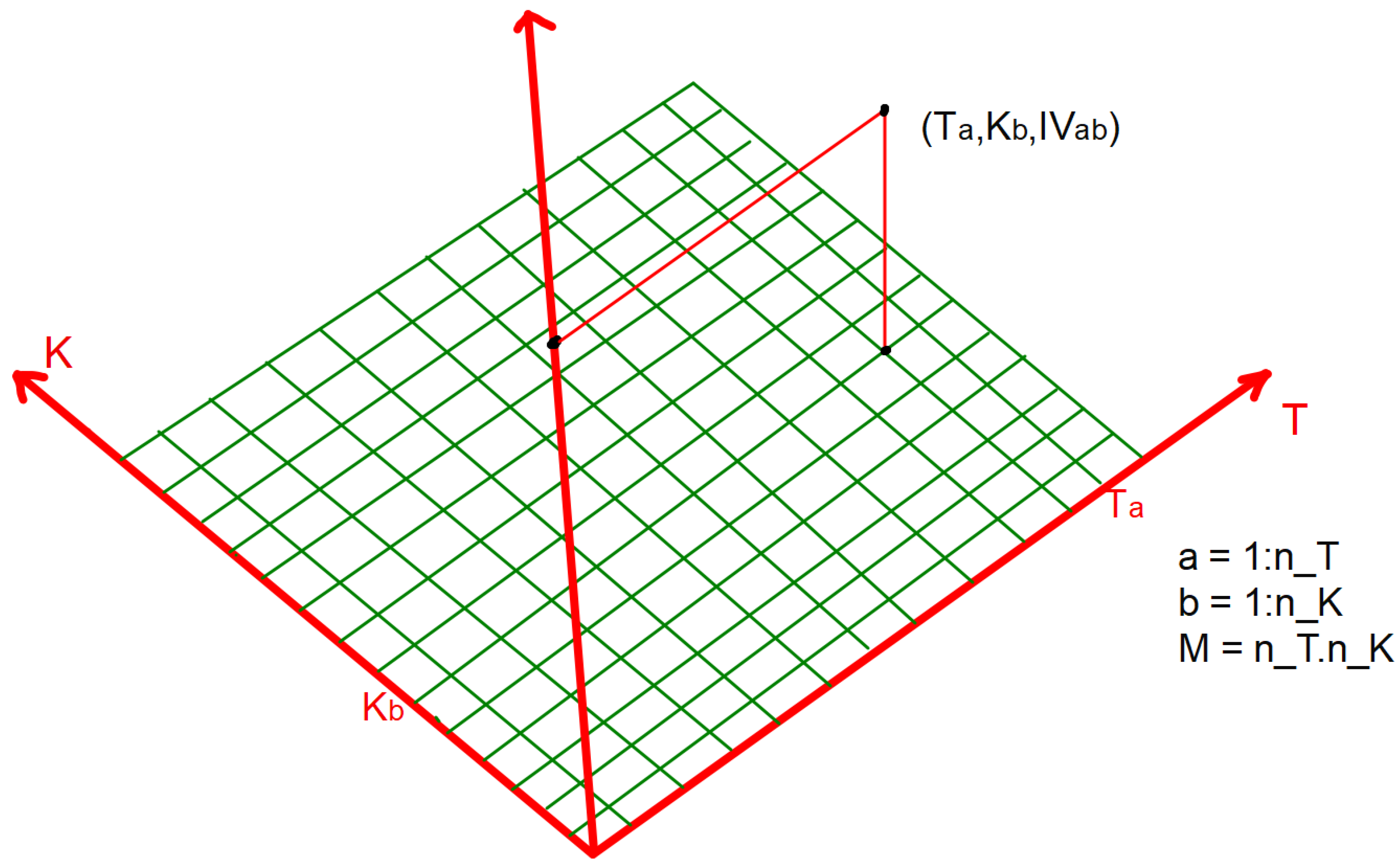
Figure 3.
Encoding the surface, .
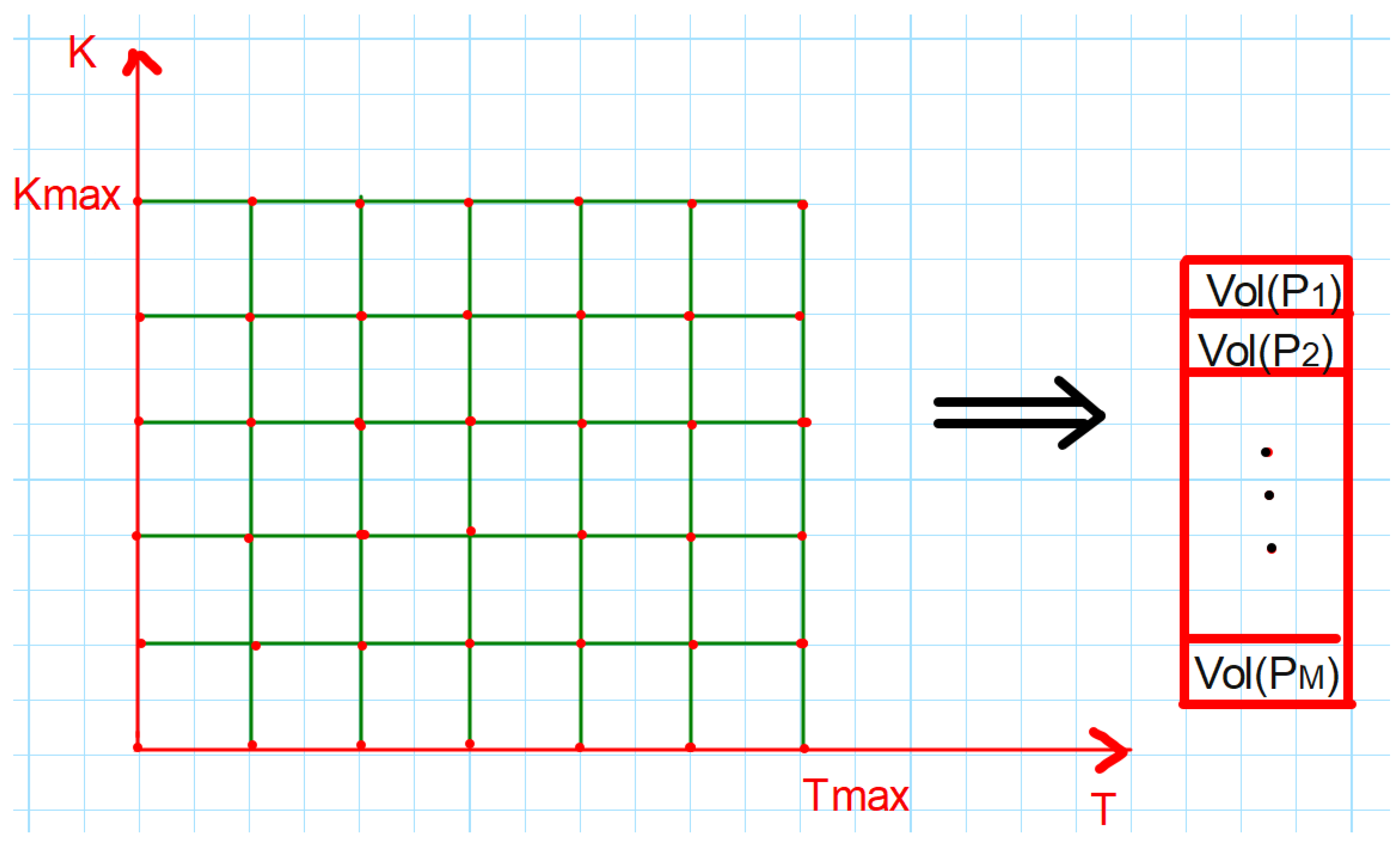
Figure 4.
Holed surface to be completed.
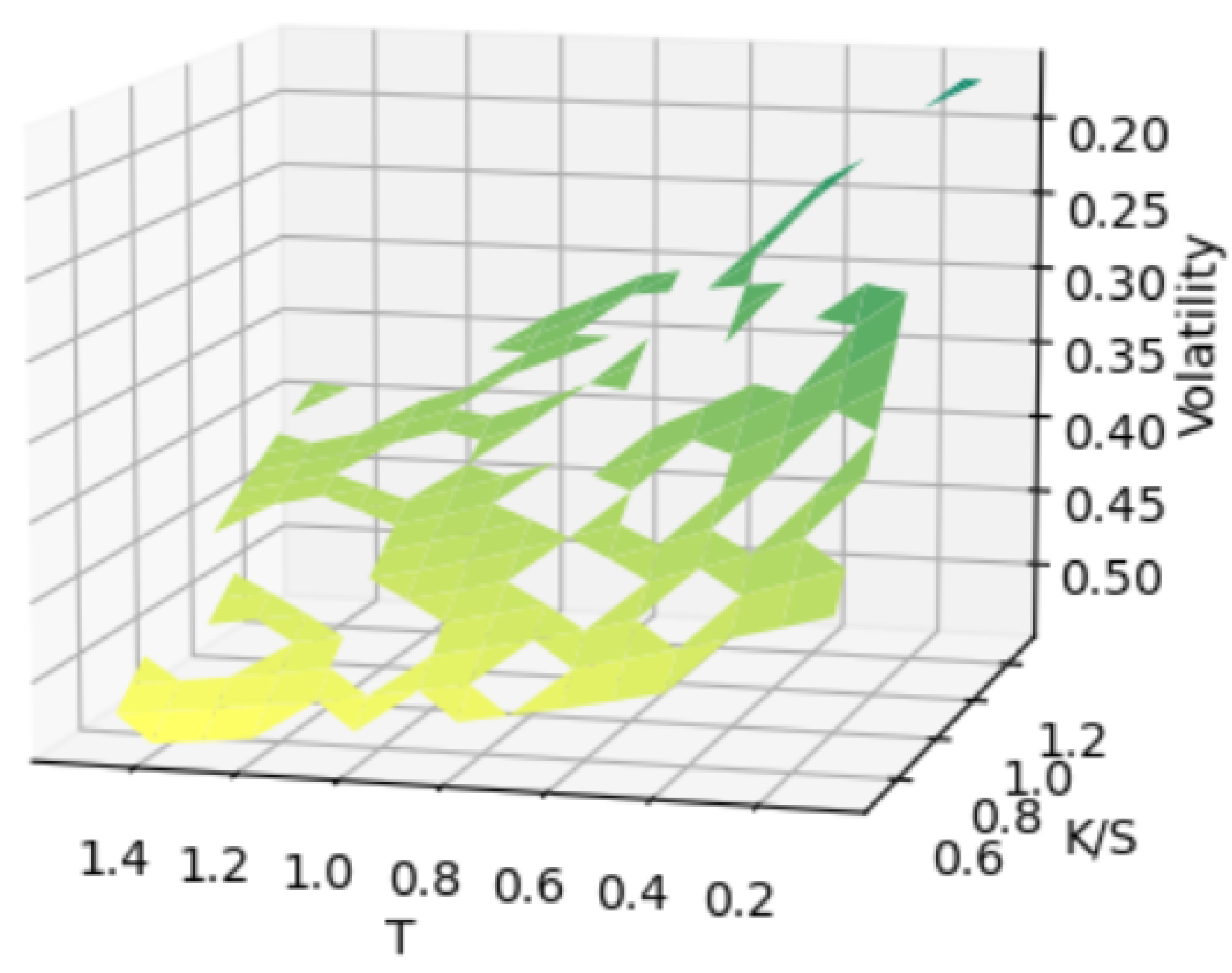
Figure 5.
Reconstructed surface and the original.
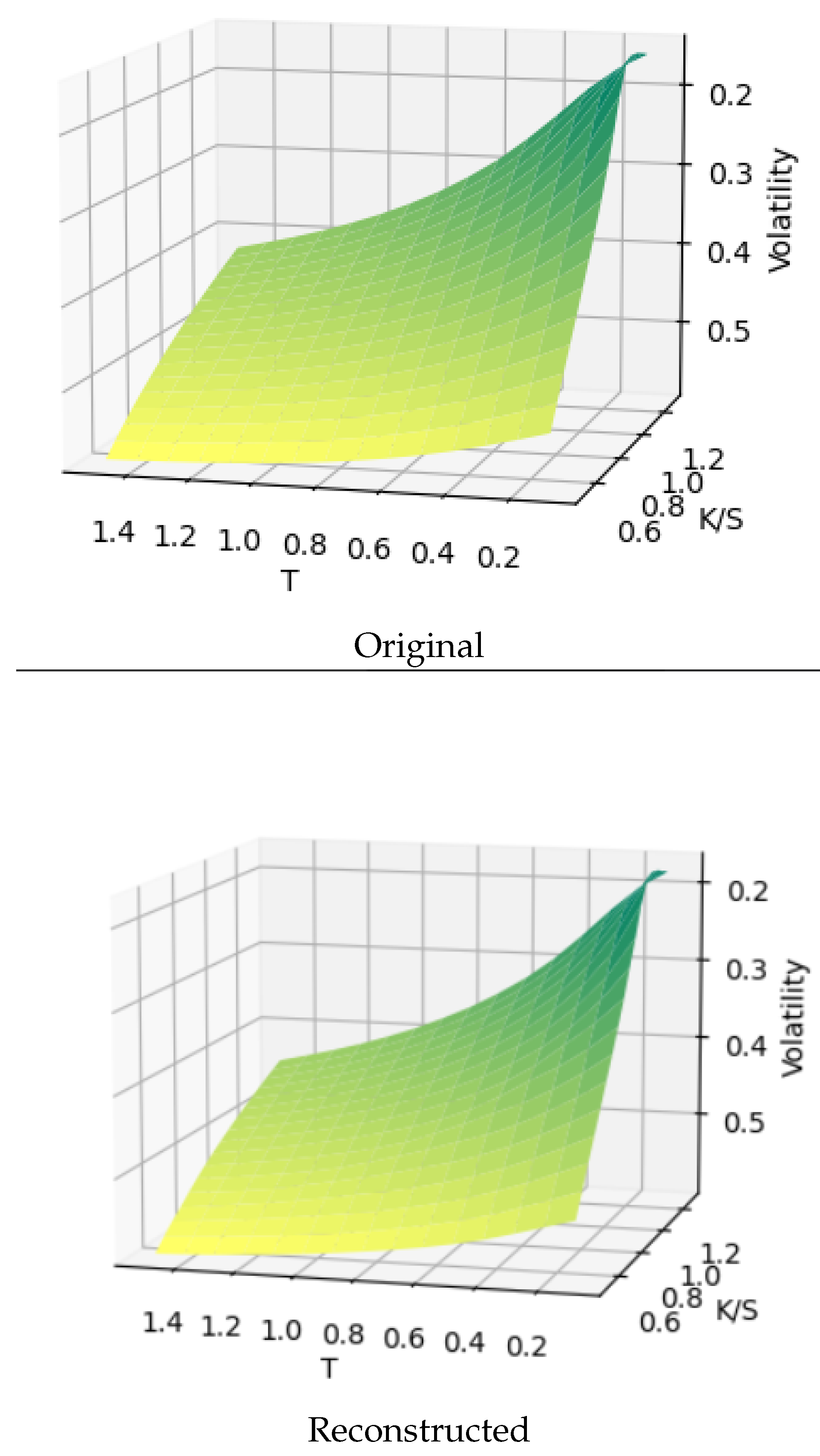
| Original |
| Reconstructed |
Figure 6.
Heston volatility surface with 100 holes reconstructed by simple reconstruction.
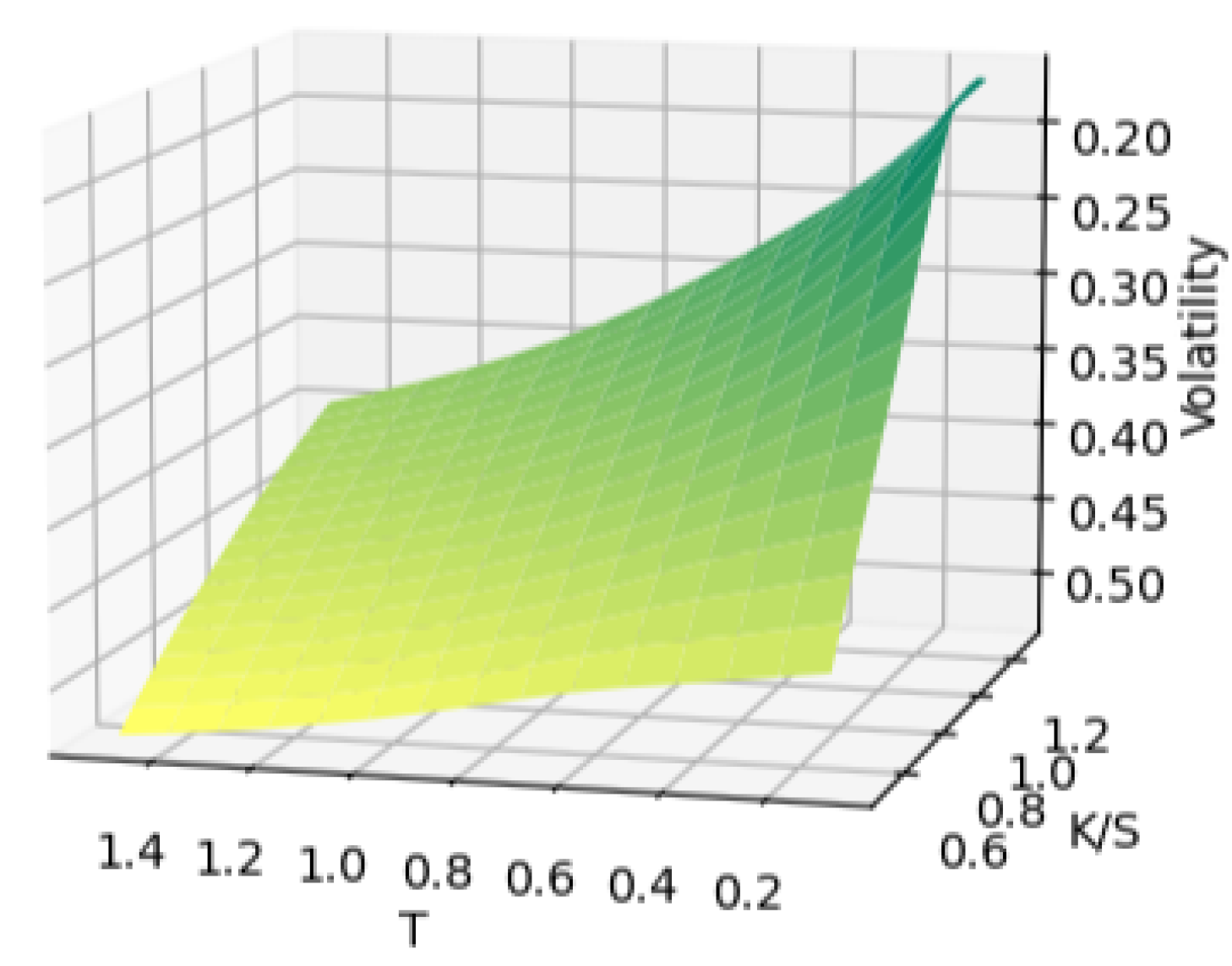
Figure 7.
Heston volatility surface with 100 holes reconstructed via latent space optimization.
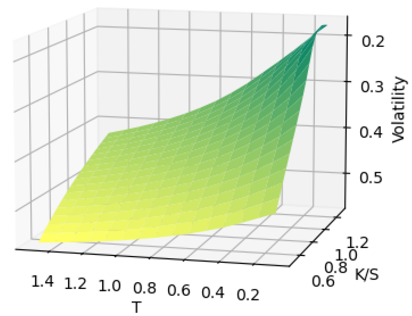
Figure 8.
Strips of reconstructed surface with the original and the incomplete one from the training set.
Figure 8.
Strips of reconstructed surface with the original and the incomplete one from the training set.
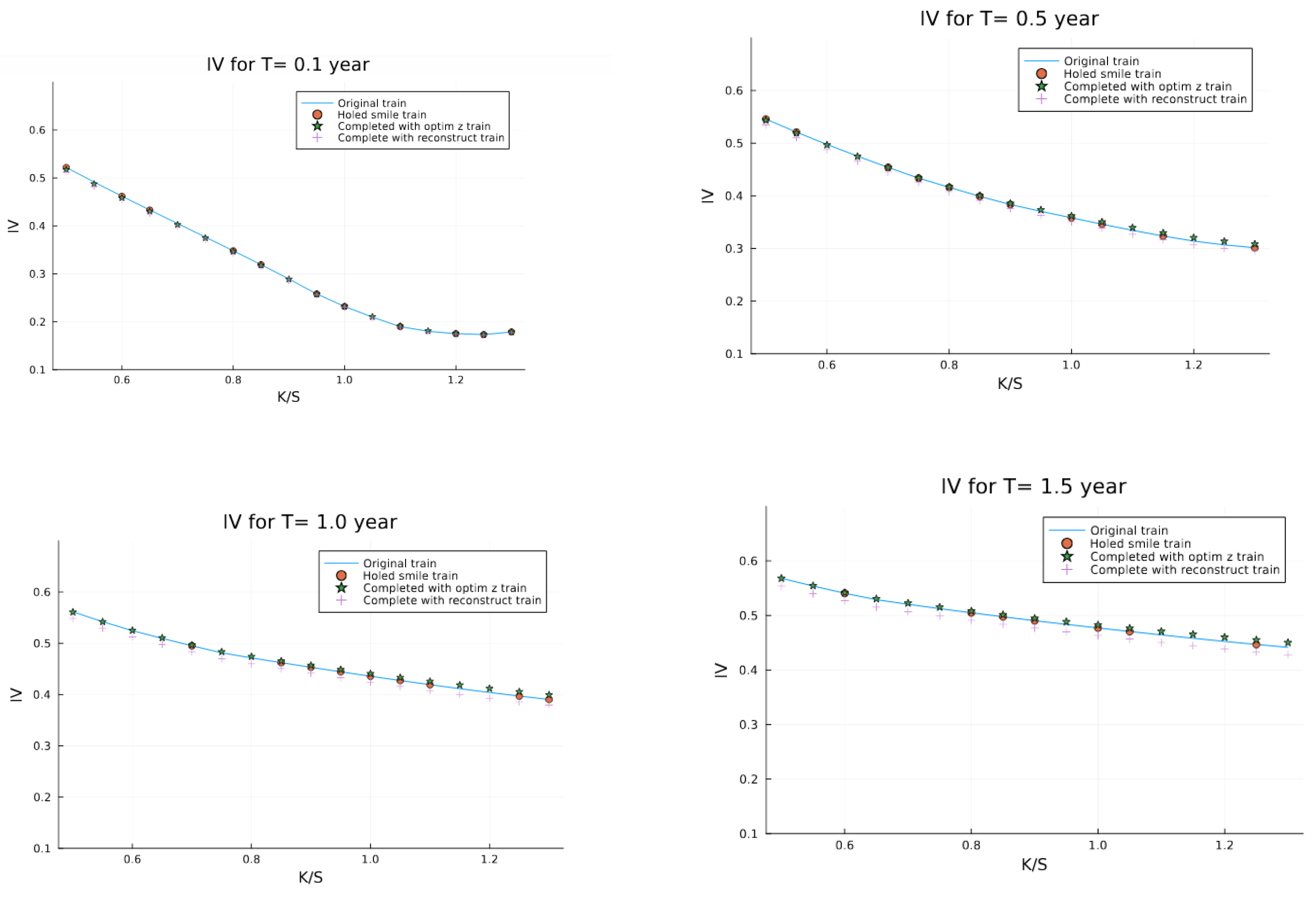
Figure 9.
Strips of reconstructed surface with the original and the incomplete one from the validation set.
Figure 9.
Strips of reconstructed surface with the original and the incomplete one from the validation set.
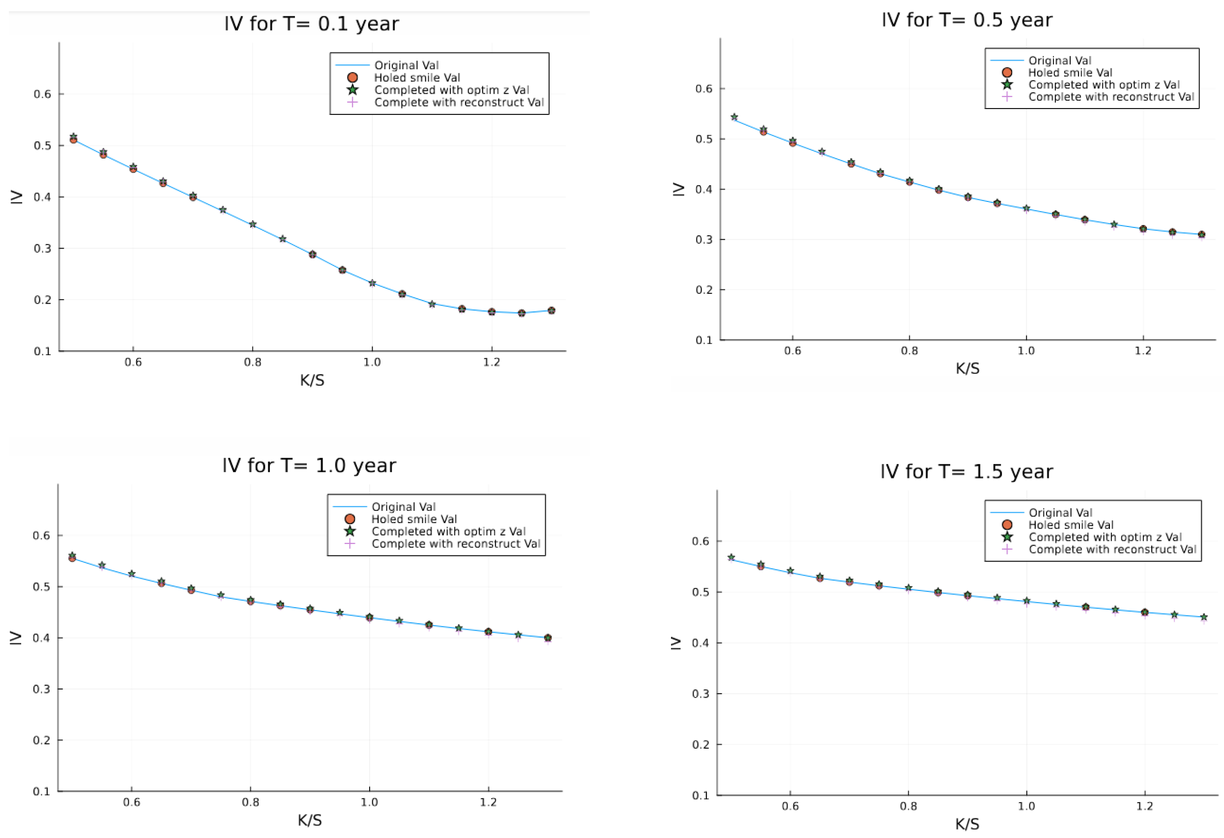
Figure 10.
The representation of the probability distribution for implied volatility shows no butterfly arbitrage.
Figure 10.
The representation of the probability distribution for implied volatility shows no butterfly arbitrage.
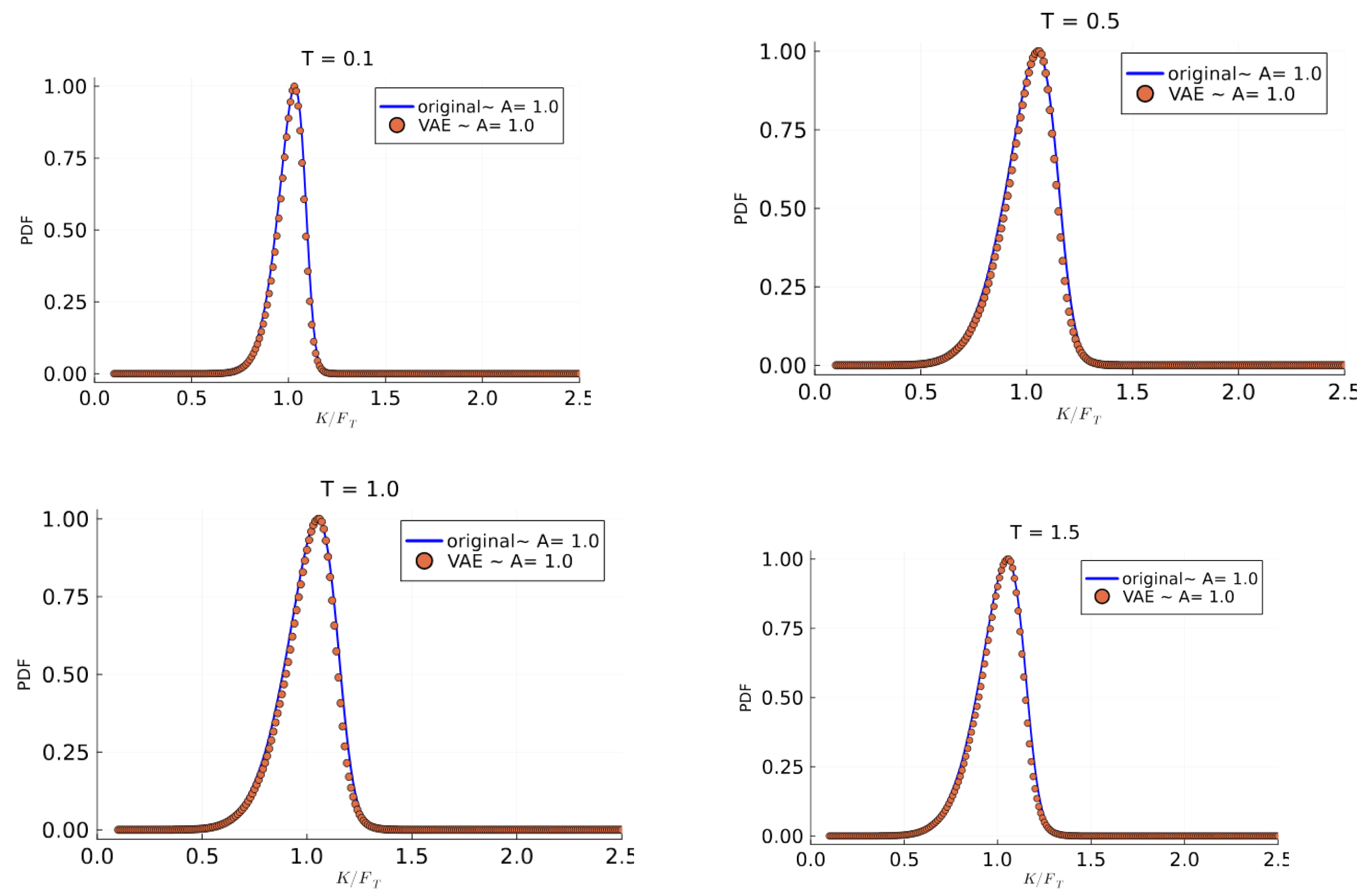
Figure 11.
Graphical representation shows no calendar Arbitrage.
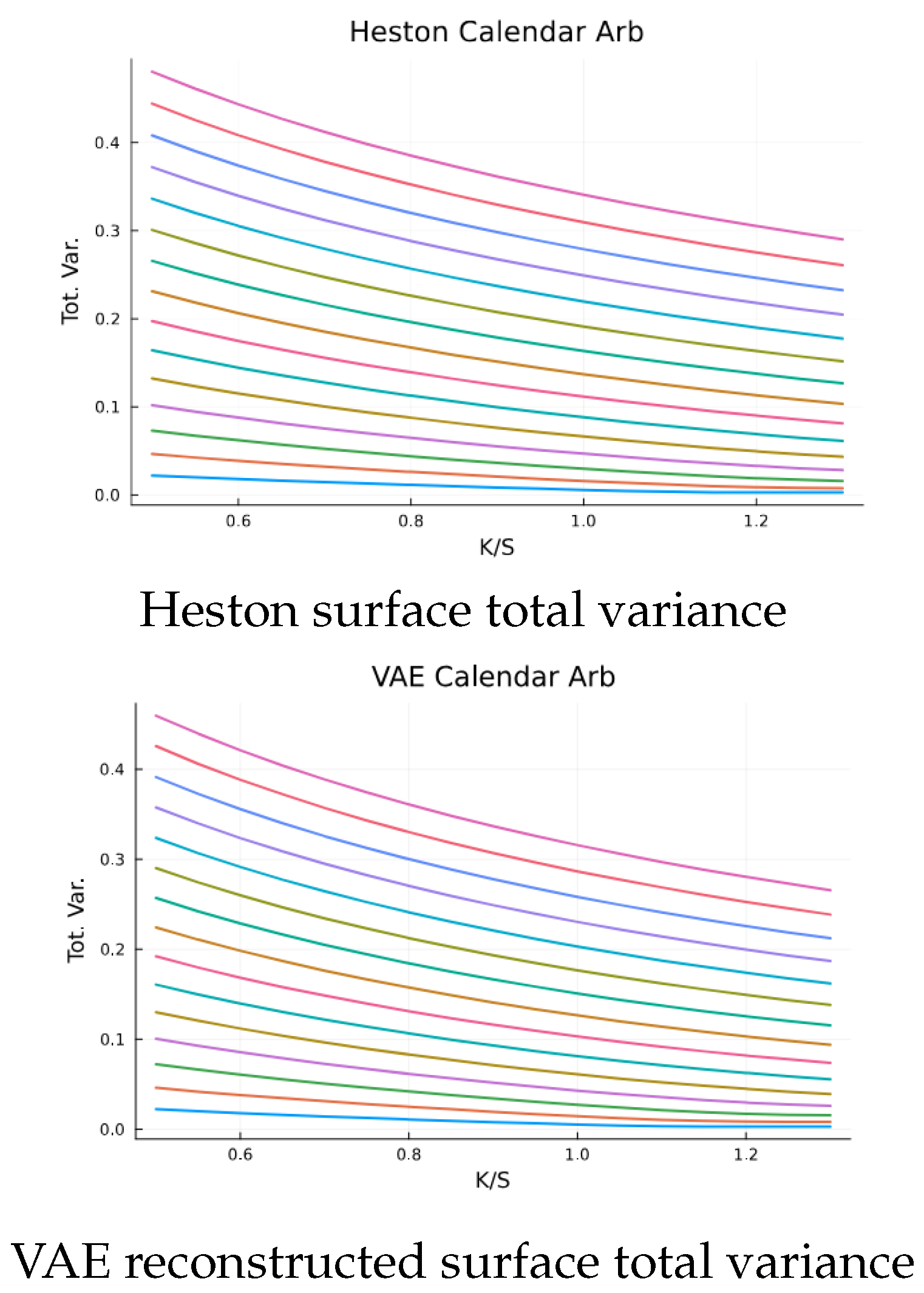
| Heston surface total variance |
| VAE reconstructed surface total variance |
Table 3.
Comparison of reconstruction errors between standard reconstruction and latent optimization approaches for different percentages of missing data points.
Table 3.
Comparison of reconstruction errors between standard reconstruction and latent optimization approaches for different percentages of missing data points.
| % holes | nbr of holes | Training set | Validation set | ||
| Error Recons | Error Latent Opt | Error Recons | Error Latent Opt | ||
| 20% | 51 | 5 | 3.71 | 3.619 | 3.616 |
| 40% | 102 | 6.59 | 3.91 | 3.62 | 3.616 |
| 60% | 153 | 6.59 | 4.39 | 3.621 | 3.617 |
| 80% | 204 | 1.008 | 5.40 | 3.621 | 3.617 |
| 96% | 243 | 1.95 | 5.21 | 3.622 | 3.617 |
Disclaimer/Publisher’s Note: The statements, opinions and data contained in all publications are solely those of the individual author(s) and contributor(s) and not of MDPI and/or the editor(s). MDPI and/or the editor(s) disclaim responsibility for any injury to people or property resulting from any ideas, methods, instructions or products referred to in the content. |
© 2025 by the authors. Licensee MDPI, Basel, Switzerland. This article is an open access article distributed under the terms and conditions of the Creative Commons Attribution (CC BY) license (http://creativecommons.org/licenses/by/4.0/).
Copyright: This open access article is published under a Creative Commons CC BY 4.0 license, which permit the free download, distribution, and reuse, provided that the author and preprint are cited in any reuse.


