Submitted:
18 February 2025
Posted:
19 February 2025
You are already at the latest version
Abstract
Accurate forecasting of construction material prices is essential for effective cost control and risk management in construction projects. However, due to the influence of various complex factors, building material prices exhibit high nonlinearity and instability, making traditional prediction methods often inadequate for achieving optimal results. This study introduces an innovative prediction model, CEEMDAN-VMD-GRU-ARIMA, specifically designed for forecasting the price of prestressed steel bars. This model uniquely combines CEEMDAN and VMD to address nonlinear characteristics, and it innovatively incorporates sample entropy for the adaptive selection of either GRU or ARIMA for prediction. Additionally, a VMD decomposition mode number K value optimization method based on a sparse index is proposed. Experimental results demonstrate that the model performs exceptionally well, achieving an Adjusted R-squared value of 0.81, with various error indicators significantly surpassing those of the baseline model. This approach offers new insights for short-term price prediction of building materials and contributes to enhancing the economic benefits and management efficiency of construction projects.
Keywords:
Construction material price forecasting
; CEEMDAN-VMD-GRU-ARIMA
; Nonlinear time series
; Sample entropy
; Prestressed Steel Bars (PSB)
1. Introduction
The revitalization of historical urban districts and the enhancement of living standards within the real estate sector play a pivotal role in driving national economic growth [1]. The selection and management of building materials, serving as the physical foundation of the construction industry, significantly impact the cost estimation of construction projects[2]. Effective cost management is not only crucial for developers but also essential for the successful execution of real estate ventures[3]. In recent years, the Chinese real estate market has experienced contraction, prompting a heightened focus on cost accounting within the industry. The pricing of building materials is influenced by multiple interrelated factors, including market dynamics, production costs, macroeconomic conditions, political climates, and environmental policies[4,5]. These factors contribute to nonlinear price fluctuations that cannot be effectively predicted using simple additive principles. Consequently, accurately forecasting building material prices poses a substantial challenge for developers, who must ensure the economic viability of their projects. To address this challenge, developers must adopt sophisticated forecasting methods and tools capable of accounting for the complex and dynamic nature of building material pricing. Additionally, they must stay informed about market trends, regulatory changes, and other external factors that may impact material costs. By employing such strategies, developers can make informed decisions and mitigate the risks associated with cost overruns, ultimately contributing to the success of their real estate ventures and supporting broader economic development.
Time series forecasting is a powerful analytical tool that uncovers and predicts future trends and patterns of evolution by deeply mining and analyzing historical data. This method has been widely applied in various fields such as finance[6], meteorology[7], transportation[8], and healthcare[9], proving its outstanding ability in predicting the future. In the field of building material price forecasting, time series forecasting also plays a crucial role, providing profound analytical tools for stakeholders and helping decision-makers make wiser decisions. However, the fluctuation of building material prices is a complex process that gradually emerges over time and is jointly influenced by various factors such as seasonal factors, market supply and demand relationships, raw material costs, policy adjustments, and the global economic environment. By accurately analyzing the historical data of building material prices, precise forecasting models can be constructed to discover the internal laws of price changes, thereby providing forward-looking guidance for market participants[10]. Forecasting models not only help developers and investors to avoid risks and optimize resource allocation but also provide decision support for policymakers to promote market stability and healthy development. Early forecasting models for building material prices were mostly based on traditional statistical methods. For example, Svetlana S. Uvarova et al. used the Autoregressive Integrated Moving Average (ARIMA) time series model to conduct an in-depth forecast analysis of the dynamic changes in steel prices[11]. This study not only provided a scientific forecasting tool for the fluctuations in steel prices but also offered practical guidance for actual construction in the construction industry. By accurately predicting the trend of steel price fluctuations, construction companies can better control costs and manage risks, thereby improving construction efficiency and economic benefits. Jiang, F. et al. carefully constructed the ARIMA time series model to conduct an in-depth forecast analysis of the Construction Cost Index (CCI)[12]. They not only accurately constructed the model but also comprehensively and meticulously discussed the various factors affecting the CCI. The purpose of this study is to enhance the accuracy of decision-makers in predicting building material prices and labor costs, thereby providing solid data support and decision-making basis for cost control and risk assessment in the construction industry. Ilbeigi, M. et al. proposed four time-series forecasting models: Holt Exponential Smoothing, Holt-Winters ES, ARIMA, and SARIMA, and confirmed that these models have better predictive performance for asphalt cement prices than existing forecasting models, thereby reducing the cost impact caused by asphalt cement price fluctuations in construction projects[13]. Although the above studies are based on traditional statistical models for building price index forecasting models, these models have limitations in dealing with nonlinear historical nodes in time series, leading to unsatisfactory prediction accuracy. To overcome this challenge, researchers need to explore more advanced methods, such as machine learning and deep learning technologies, to improve the accuracy and adaptability of forecasting models. By continuously optimizing and innovating, time series forecasting will play a greater role in the field of building material price forecasting, providing more accurate forward-looking guidance for market participants.
With the rapid advancement of big data and artificial intelligence technologies, methods for time series forecasting are continuously being innovated and refined. Modern forecasting models, such as those based on deep learning architectures like Long Short-Term Memory networks (LSTM)[14], Convolutional Neural Networks (CNN)[15], and Large Language Models (LLM)[16], have demonstrated exceptional performance in handling complex, nonlinear time series data. The broad application of these technologies further enhances the accuracy and reliability of building material price forecasting, providing more solid data support for decision-making in related fields. The introduction of deep learning technology has ushered in new breakthroughs in the field of time series forecasting. Deep learning models, particularly LSTM and CNN, are capable of automatically extracting complex features from time series data, capturing long-term dependencies and nonlinear patterns within the data. For instance, Tang, B.Q. et al. innovatively combined an Improved Particle Swarm Optimization algorithm (IPSO) with Least Squares Support Vector Machines (LSSVM) to develop an efficient building material price forecasting model[17]. Compared with traditional neural networks and traditional time series models, this method showed significant advantages: the mean relative error and mean square error were significantly reduced, confirming its outstanding performance in prediction accuracy, convergence speed, and generalization capability. This advanced forecasting method not only accurately predicts building material prices but also helps determine the optimal purchase timing, effectively reducing cost impacts. By accurately predicting the fluctuations in building material prices, construction companies and developers can better plan procurement strategies, optimize inventory management, mitigate risks associated with price volatility, and enhance economic benefits. Mir, M. et al. addressing the shortcomings of machine learning models in precision estimation, proposed an innovative Optimal Lower and Upper Bound Estimation (Optimal LUBE) method[18]. This method, by training Artificial Neural Networks (ANN), can output precise prediction error intervals, significantly enhancing the accuracy of decision-making. This groundbreaking result not only greatly reduced project cost risks but also brought a new research perspective and direction to the construction industry. Wang, J. et al. used K Nearest Neighbors (KNN) and Perfect Random Tree Ensemble (PERT) algorithms to conduct in-depth short-term, medium-term, and long-term forecasting analysis of the CCI[19]. By comparing with existing forecasting models, they successfully demonstrated the significant advantages of the proposed method in predictive performance, providing valuable auxiliary decision-making tools for contractors and owners, enabling them to budget and control costs more accurately. The introduction of the above machine learning models greatly improved the accuracy and robustness of predictions. Furthermore, the application of Large Language Models (LLM) also provides a new perspective for time series forecasting, especially when dealing with time series data with rich semantic information, enabling a better understanding of the logic and patterns behind the dataset[20]. Although machine learning models have made significant performance improvements, they still face the challenge of underfitting. The main reason for this issue is the presence of noise, which makes traditional statistical models and deep learning models difficult to accurately fit historical building material prices, and thus unable to accurately predict future price trends. To address the above issues, this study employed advanced Complete Ensemble Empirical Mode Decomposition with Adaptive Noise (CEEMDAN) and Variational Mode Decomposition (VMD) techniques for denoising of building material prices. On this basis, this study further combined GRU networks and ARIMA time series forecasting models for more accurate predictions of building material prices. The precision and dependability of these forecasting outcomes are pivotal to the successful and punctual execution of construction projects. Moreover, they offer substantial support for the enduring growth and sustainability of the construction sector, ensuring that it remains at the forefront of innovation and efficiency.
2. Data Sources and Analysis
2.1. Data Source
The experimental data in this study is obtained from the Zhengzhou Construction Project Cost Management Information, a reputable source known for its consistent and reliable monthly updates on construction material prices. In particular, our research focused on gathering monthly price for PSB from the years 2008 to 2023. To address any gaps in the collected data, we employed the Akima Hermite Interpolation (AKIMA) algorithm for data imputation[21]. The resulting price distribution diagram of the preprocessed PSB is illustrated in Figure 1.
In Figure 1, which is clear that the pricing distribution of PSB exhibits a noticeable imbalance. The majority of prices are concentrated in the 4000~5000RMB/ton range, indicating a significant clustering in this particular region. Conversely, there is a distinct lack of prices falling within the 2000~3000 RMB/ton and 6000~7000RMB/ton brackets. This uneven distribution underscores the considerable variability inherent in the pricing data for PSB. As a result, this poses challenges for accurately predicting the prices of PSB.
2.2. Data Analysis
To delve deeply into the patterns of change in the time series data of PSB prices, we leverage the capabilities of Eviews8.0 to meticulously examine the trend characteristics within the price time series data for PSB. The outcomes of our application of the Hodrick-Prescott (HP) filter model to this price time series are elegantly presented in Figure 2. For the HP filter model, the parameter λ has been meticulously calibrated to a value of 14400, adhering to the well-established empirical rule of thumb, which is particularly suited for the analysis of long-term economic time series data[22]. This strategic choice facilitates an accurate and insightful extraction of the intrinsic trend from the dataset.
Figure 2 presents a detailed time series analysis of PSB, revealing long-term trends and periodic fluctuations. The trend sequence identifies key elements of pre-stressed steel bars associated with the overall trend, while the cycle sequence emphasizes regular fluctuations. Data indicates a downward price trend from 2008 to 2015, an upturn from 2016 to 2022, and a subsequent decline, suggesting a potential future decrease in prices. This could significantly impact China's construction industry by reducing construction costs, stimulating market growth, and increasing demand, potentially attracting more investors. However, the broader implications on market dynamics require consideration, as price reductions may lead to complex industry interactions and adjustments.
3. Methods
Material prices are a critical determinant of construction project costs and exhibit significant randomness. To enhance the accuracy and predictability of future predictions for the prices of PSB, this study employs machine learning techniques to construct an innovative model for forecasting the prices of PSB. The model has been rigorously validated to demonstrate its predictive capabilities. The study commenced with a comprehensive statistical analysis of the collected data on the prices of PSB. Missing values within the dataset were effectively addressed using the AKIMA algorithm. Subsequently, the dataset was partitioned into training and testing sets in a 4:1 ratio, laying the groundwork for the subsequent construction of a time series prediction model. Following this, the training set data were fed into the constructed prediction model, and five iterations of optimization were performed to identify and determine the optimal model parameters. The effectiveness of the model was then validated by inputting the test set data into the model. Ultimately, this study selected four popular machine learning time series prediction models and compared them with the integrated model developed in this study, further validating the model's predictive performance and effectiveness. For a detailed framework structure of the study, refer to Figure 3.
3.1. Integrated Decomposition-Ensemble Model for PSB Market Price Prediction
To enhance the precision of the price forecasting model for PSB, we introduce an innovative integrated prediction model that builds upon the theoretical framework of model decomposition and fusion models[23]. This model leverages the synergistic application of CEEMDAN and VMD, complemented by ARIMA and GRU Networks. Below, we delineate the foundational principles that underpin the integration of these methodologies within our models.
3.1.1. CEEMDAN Model
Influenced by various factors such as policy, environment, and economy, the price of PSB is subject to significant noise. To mitigate the impact of noise on model learning, this study utilizes Complete Ensemble Empirical Mode Decomposition with Adaptive Noise (CEEMDAN) with Adaptive Noise for analyzing PSB. CEEMDAN, an adaptive noise control signal decomposition method derived from Complete Ensemble Empirical Mode Decomposition (CEEMD) and Ensemble Empirical Mode Decomposition (EEMD), employs adaptive control and integration strategies to manage the construction and addition of random noise and average EEMD decomposition structure. This approach reduces the influence of random noise on results, enhancing the stability and accuracy of the decomposition outcomes[24]. In comparison to wavelet and Fourier transform methods, CEEMDAN demonstrates notable advantages in data stationarity testing and linearity. As a time-domain analysis technique, CEEMDAN effectively minimizes reconstruction errors by progressively reducing noise in the dataset, with its efficacy confirmed through multiple experiments[25].
3.1.2. ARIMA Model
ARIMA, as a traditional time series forecasting model, has become widely used for its simplicity and ease of understanding. By applying autoregressive, moving average, and difference processing to time series data, the ARIMA model can effectively identify future changes and provide technical support for predicting future price fluctuation[26]. To construct an ARIMA model, three parameters must be specified: the autoregressive order (p), the difference order (d), and the moving average order (q). The stationarity of the data is evaluated using an ADF test, and the optimal values for parameters p and q are determined using the Akaike Information Criterion (AIC) and Bayesian Information Criterion (BIC) [27]. The polynomial representations of the autoregressive and moving average processes are presented in equations 1 and 2, while the ARMA(p,q) is represented in equation 3.
In the above equation, therepresents the current value, μ is the constant term, p is the order, is the autocorrelation coefficient, andrepresents the error term.
3.1.3. VMD Model
VMD is a signal decomposition algorithm based on empirical mode decomposition, which is capable of adaptively processing time series data[28]. This study suggests that VMD decomposition can effectively extract high-to-moderate complex components that may not be fully decomposed using CEEMDAN, thereby reducing the complexity of the data. However, the main challenge in VMD mode decomposition lies in determining the optimal value of K, which directly affects the effectiveness of signal variation. To address this challenge, the Sparse Index optimization algorithm is employed to determine the K value for VMD mode decomposition, with the maximum sparse index value selected as the optimal K value[29]. When calculating the sparsity of different modes generated by VMD decomposition, the varying capabilities of different mode decomposition variables are taken into consideration, and the energy full time factor is introduced. Finally, the average value of marginal spectral sparsity is determined to enhance the robustness and effectiveness of VMD decomposition against the noise.
The signal obtained from VMD decomposition consists of Intrinsic Mode Functions (IMFs) that exhibit specific frequencies and frequency bands. The generated components are iteratively processed using the alternating direction multiplier algorithm (ADMM)[30] to update the center frequency of their decomposition. This process ultimately leads to the determination of the saddle point of the unconstrained model, which represents the optimal solution for the VMD decomposition problem. The implementation of the VMD algorithm primarily involves constructing the variational model and solving the associated variational problem.
The process of constructing the variational model involves combining all the IMFs as the input signal and summing the frequency bands of the IMFs to form the objective function. The original signal is then inputted, and the Hilbert transform is applied to K IMFs. The calculation equation is as follows:
In the equation 4, therepresents the generated IMFs, where k=1,2,...,K. Therepresents the central frequency of the IMFs. Therepresents the unit impulse function. Therepresents the first derivative of a function with respect to time. By incorporating the Lagrange function, the aforementioned model is refined into the optimal solution for the unconstrained problem, as depicted in the specific equation below in equation 5.
In the equation 5, the α denotes the quadratic penalty factor utilized for constraining the frequency band, while λ stands for the Lagrange multiplier. Equation 3 signifies the convergence criterion.
In the equation 6, where ε is the precision control value, which is used to limit the relative error.
3.1.4. GRU Network
A neural network is a digital and computational model that emulates the structure of a biological neural network. It is composed of numerous interconnected neurons with associated weights[31]. Initially, artificial neural networks (ANNs) were prevalent, comprising an input layer, hidden layers, and an output layer. However, to address certain challenges, deep neural networks like LSTM, TCN, CNN-LSTM[32]. These networks are prone to gradient vanishing issues but have demonstrated superior performance in non-linear fitting compared to traditional statistical methods[33]. Consequently, they have found extensive applications across various domains.
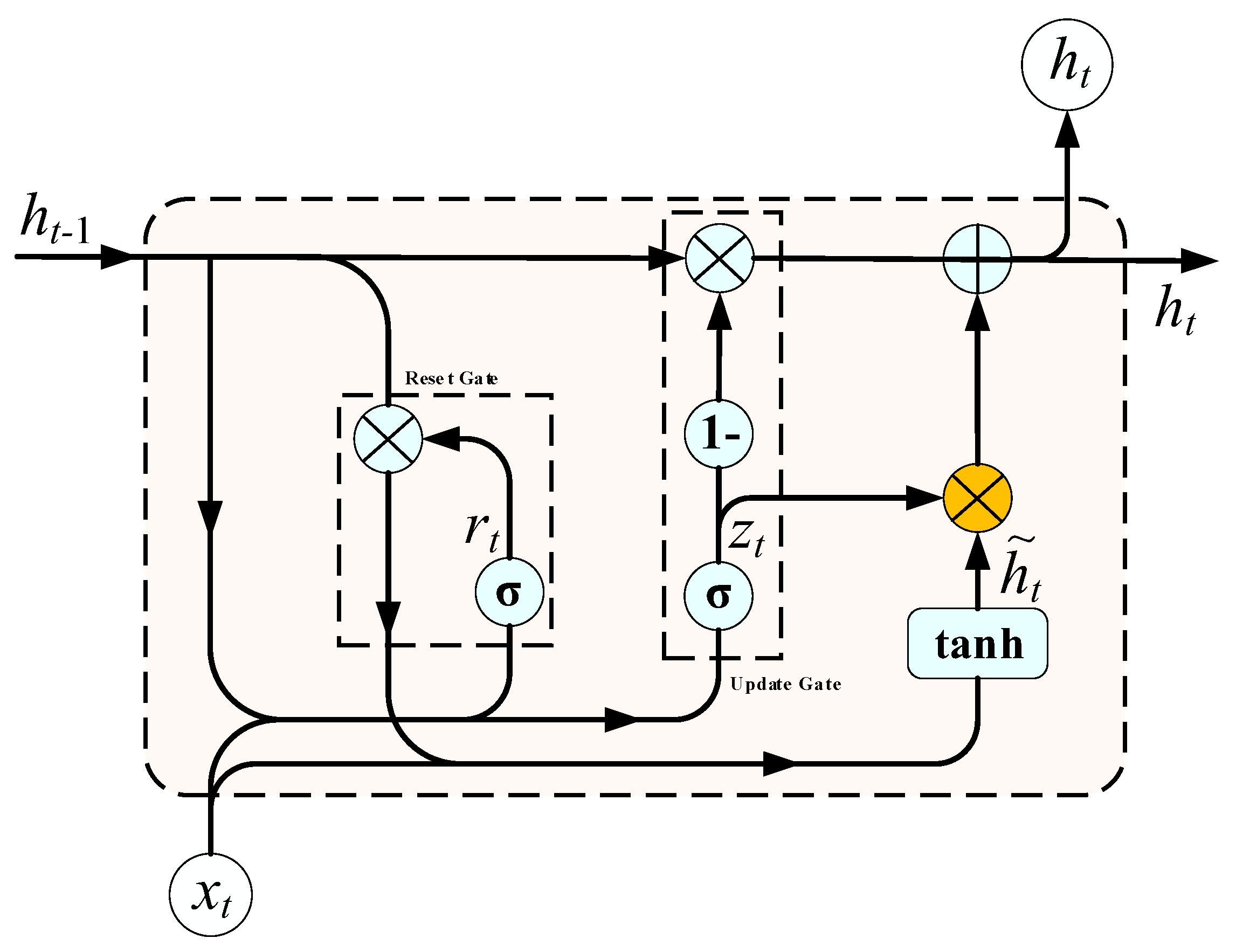
The GRU Network is a type of Recurrent Neural Network(RNN) and a simplified variant of the LSTM network[34]. It combines the forget and input gates of the LSTM network into a single update gate, which controls the retention of historical information. Additionally, it retains the reset gate of the LSTM network, which determines the current state and historical information. Compared to LSTM and TCN networks, GRU offers several advantages in effectively extracting information from time series data, thereby reducing training time and improving model performance. Figure 3 provides a schematic representation of the GRU architecture, elucidating its intricate design. The underlying mathematical equation that governs the GRU's operation is delineated as follows:
In the equation, theandrepresent the update gate and the reset gate, respectively. The update gate controls how much information from the previous time step is incorporated into the current state. A higher update gate value means more information from the previous time step is included in the current state. Theandare the output states of the current and previous hidden layers, respectively. Therepresents the combined relationship betweenand. The σ is the sigmoid activation function, while, , and are the zero output matrix, reset gate weight matrix, and update gate weight matrix, respectively.
Figure 4.
GRU Network structure.
In conclusion, we have developed an integrative and advanced forecasting model specifically designed to predict PSB price dynamics. Our methodology is characterized by systematic precision and rigorous implementation to enhance the model's comprehensiveness and predictive accuracy. The model architecture, depicted in Figure 5, demonstrates its potential to advance research in materials economics and market analysis. In the initial phase, we preprocessed price data and implemented CEEMDAN decomposition using the PyEMD package in Python 3.8.0. Subsequent sample entropy (SE) testing identified components with significant variation, ensuring complete decomposition. A threshold of 0.5 was applied to evaluate time series complexity: components with SE values exceeding 0.5 underwent VMD based secondary decomposition and GRU network prediction, while those below 0.5 were analyzed via the ARIMA model. Finally, the forecast integrates weighted summations of IMF components derived from all methods, yielding robust predictions of PSB price trends.
3.2. Model Evaluation Index
To rigorously validate the precision and dependability of our predictive model, we have chosen to compare it with four benchmark models through a comparative analysis. During this evaluation, we will employ Adjusted R-square, Mean Squared Error (MSE), Mean Absolute Error (MAE), and Root Mean Squared Error (RMSE) as the critical metrics for assessing model performance. A holistic consideration of these metrics will allow us to thoroughly evaluate the effectiveness of the predictive model and ensure its accuracy and stability when applied in practical scenarios. The Adjusted R-square indicates the model's data fit, with the MSE and RMSE measuring the variance between the model's forecasts and actual observations. The MAE evaluates the average discrepancy between the predicted and actual values. By comparing these metrics, we can more precisely determine the performance of the predictive model. The calculation equation is described as follows:
In the equation, represents the true price of the PSB, represents the predicted price of the PSB, N denotes the number of samples, and p denotes the number of feature indicators considered.
4. Result
4.1. Predicted Model Training Results
As previously discussed, the pricing of building materials is subject to a multitude of influences, including market fluctuations, external factors, and the size of the data sample. Consequently, accurately predicting these prices remains a significant challenge. While the ARIMA model has traditionally been utilized for time series forecasting in this area, its limitations in capturing nonlinear patterns have led to suboptimal performance in predicting building material prices. To address this issue, time series decomposition has emerged as a powerful tool in various fields, such as stock markets[35], environmental research[36], and fault diagnosis[37]. By breaking down the original series into trend, seasonality, and residual components, this method offers a more comprehensive understanding of the underlying structure and characteristics of the data, ultimately improving predictive accuracy. CEEMDAN, a time series decomposition algorithm, demonstrates superior adaptivity and noise control compared to wavelet decomposition, EMD, and EEMD. The five model components generated by CEEMDAN decomposition in Figure 5, exhibit a significant reduction in nonlinearity and randomness in the decomposed subsequence of PSB price.
However, the CEEMDAN model is susceptible to noise interference during signal decomposition, potentially compromising the accuracy of the decomposition results. To mitigate the impact of noise on the model, this study proposes the utilization of Sample Entropy (SE)[38] to assess the complexity and uncertainty of the model components CEEMDAN decomposition, with a predefined threshold of 0.5. The SE exceeding 0.5 indicates incomplete signal decomposition by CEEMDAN, whereas a value below 0.5 signifies successful signal decomposition. This approach enables a more precise evaluation of CEEMDAN decomposition efficacy and facilitates further optimization of the model's performance. For sample entropy calculation results in Figure 6.
In Figure 7, the model component 1 and model component 2 generated by the CEEMDAN decomposition exhibit high SE values, both exceeding 0.5. This indicates that IMFs1 and IMFs2 possess a certain level of complexity and uncertainty. To mitigate the impact of this complexity and uncertainty on the model learning performance, a quadratic decomposition of IMFs1 and IMFs2 is performed in this study to address the model mixing problem. While the VMD decomposition has demonstrated favorable outcomes in various fields, its decomposition effect parameters, including the model number K-value, the penalty factor α, and the Lagrange multiplier, significantly influence the results. Among these parameters, the setting of the K-value is particularly crucial.
By effectively setting the K-value and ensuring the other parameters fall within the valid range, the signal can be decomposed effectively. Therefore, the effectiveness of VMD decomposition is directly influenced by the appropriate selection of the K-value. To address the impact of the K-value on VMD decomposition, researchers have sought the optimal K-value using methods such as Energy ratio[39], Genetic Algorithm[40], and Whale Optimization Algorithm[41]. However, these methods primarily seek local optima and do not fully utilize the VMD process. In light of this, this study proposes an adaptive K-value optimized variational model decomposition based on the sparsity index during the decomposition process[42]. The SE of the VMD components under different decomposition model numbers K-value is employed as an index for optimization. The specific optimization search results are presented in Figure 7.
Figure 8, which can be inferred that the optimal parameter K-value for VMD variational modes to IMF1 and IMF2, are determined as 10 and 6, respectively, through sparse index optimization. Subsequently, this optimized K-value is utilized to decompose IMFs1 and IMFs2 using the VMD technique.
In Figure 9 and Figure 10 present the final model decomposition results for the price of PSB. The sample entropy value of the model variables obtained from the CEEMDAN decomposition is below 0.5, indicating a complete decomposition of the model. Since data with low SE have lower noise levels, to avoid issues such as overfitting during the training process of deep learning models on data with sample entropy, this study opts for the traditional statistical prediction model ARIMA for prediction. However, for the model components obtained from VMD decomposition, the deep learning model GRU is employed for prediction. The experimental training and testing datasets are divided in accordance with the mathematical and statistical specification standard of a 4:1 ratio. Finally, the variables predicted by the ARIMA and GRU models are fused using weighting, and the final testing datasets predicted prestressing rebar price results are output in Figure 9.
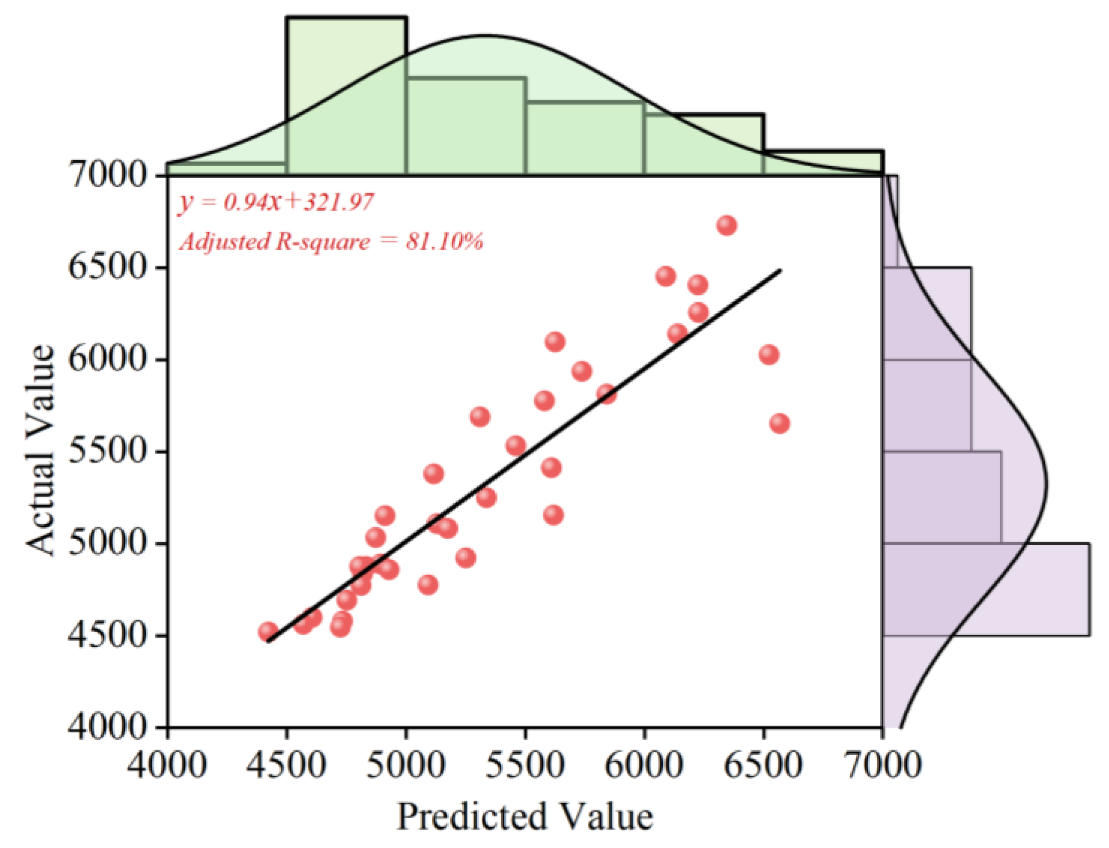
In Figure 11, the CEEMDAN-VMD-GRU-ARIMA model exhibits exceptional performance in predicting the price of PSB based on our empirical tests. The model's Adjusted R-squared value significantly exceeds 0.80, demonstrating its high precision and accuracy. Further analysis reveals that while the model generates significant inaccuracies within the price range of 4000-4500 Yuan RMB/Ton, these inconsistencies do not negatively impact its overall effectiveness or applicability. Summarizing these findings, we can confidently state that the CEEMDAN-VMD-GRU-ARIMA model is highly reliable and practically viable for short-term PSB price prediction. The model's robust performance across different price points suggests its potential as a valuable tool for real-world applications in cost management and risk mitigation strategies within construction projects.
As shown in Figure 11, empirical tests demonstrate that the CEEMDAN-VMD-GRU-ARIMA model achieves exceptional performance in predicting PSB prices, with an adjusted R² value exceeding 0.80, indicating high precision and reliability. Further analysis reveals that although the model exhibits notable inaccuracies within the 4,000–4,500 RMB/ton price range in Figure 12, these localized discrepancies do not compromise its overall effectiveness for short-term forecasting. In summary, the proposed hybrid model demonstrates robust generalizability and practical viability, particularly for cost management and risk mitigation in construction projects, where dynamic price fluctuations require timely decision-making.
4.2. Verification Predicted Models Results
The rigorous validation of our model is paramount for substantiating the veracity and authority of our research outcomes, thereby laying a robust groundwork for future policy advocacy and strategic decision-making. By conducting a meticulous examination and validation of our model, we can assert with confidence that it excels not only in capturing historical pricing data of construction materials but also in forecasting future price trajectories with a high degree of precision. The results of the test set are graphically depicted in Figure 11 and Table1. As illustrated in Figure 11, there are notable fluctuations in the model's predictive accuracy on the 1st of May 2021, the 1st of June 2021, and between the 1st of October 2021 and the 1st of February 2022. Detailed findings are delineated in Appendix 1. Such fluctuations may stem from the intricacies of the market environment or anomalies in data during these intervals. Conversely, in other periods, the model exhibits relatively minor error variance, indicative of its stability and dependability under those conditions. Upon a comprehensive analysis of the time series forecasting model, it is evident that it encounters certain constraints in the prediction of time series peaks. This limitation may arise from the model's inadequate capacity to capture outlier events or its reduced sensitivity to market volatility. Nonetheless, within more stable time series contexts, the model demonstrates superior performance.
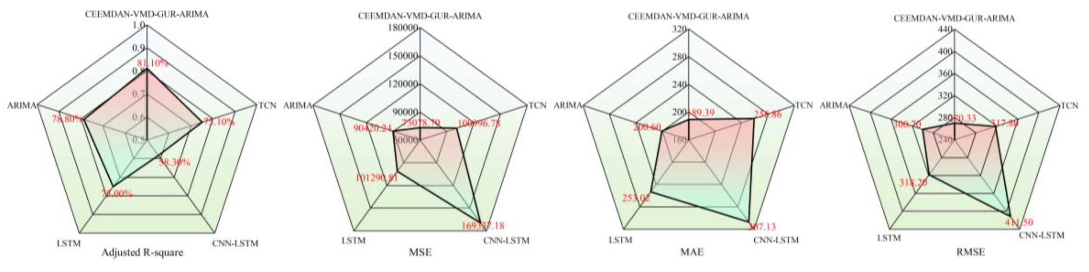
In our quest to ascertain the precision and reliability of our predictive model, we subjected it to a stringent comparative analysis against four established benchmark models, as delineated in Figure 12. This rigorous evaluation encompassed key performance metrics such as Adjusted R-square, MSE, MAE, and RMSE. Our novel CEEMDAN-VMD-GRU-ARIMA approach emerged as superior across all metrics, significantly outperforming its counterparts, with the ARIMA model securing the second position and the CNN-LSTM model exhibiting comparatively lower accuracy. These disparities can be ascribed to the distinct algorithmic attributes and the specific contexts in which each model operates within the realm of time series analysis. The CEEMDAN-VMD-GRU-ARIMA method's synergistic integration of diverse algorithms adeptly harnesses the nonlinear and dynamic intricacies of time series data, thereby augmenting its predictive prowess. In contrast, the ARIMA model, while effective in certain scenarios, encounters limitations when confronted with intricate datasets. Similarly, the CNN-LSTM model, despite its excellence in specific domains, necessitates further enhancement for adept time series forecasting. This comprehensive analysis serves as a pivotal reference for the ongoing refinement and optimization of our model, ensuring its robustness and efficacy in the evolving landscape of predictive analytics.

Table 1.
Comparative Analysis of Actual, Predicted Values, and Error Metrics.
| Date | Actual | Predict | Residuals |
| 2020-8-1 | 3520.00 | 4422.52 | 97.47 |
| 2020-9-1 | 4600.00 | 4606.04 | -6.04 |
| 2020-10-1 | 4590.00 | 4738.86 | -153.86 |
| 2020-11-1 | 4693.00 | 4750.98 | 57.98 |
| 2020-12-1 | 4890.00 | 4892.68 | -2.68 |
| 2021-1-1 | 5110.00 | 5128.93 | -18.93 |
| 2021-2-1 | 5500.00 | 5337.11 | -87.11 |
| 2021-3-1 | 5533.00 | 5459.93 | -126.66 |
| 2021-4-1 | 5640.00 | 5571.37 | 199.04 |
| 2021-5-1 | 6433.33 | 6069.67 | 363.66 |
| 2021-6-1 | 5666.67 | 6522.55 | -255.88 |
| 2021-7-1 | 5540.00 | 6139.05 | -199.05 |
| 2021-8-1 | 6256.67 | 5645.58 | 611.10 |
| 2021-9-1 | 6400.00 | 6206.27 | 193.73 |
| 2021-10-1 | 6730.00 | 6345.15 | 384.85 |
| 2021-11-1 | 6563.33 | 6587.06 | -313.73 |
| 2021-12-1 | 6155.82 | 6618.85 | -463.03 |
| 2022-1-1 | 5880.11 | 5966.36 | -86.25 |
| 2022-2-1 | 5690.00 | 5897.80 | 380.20 |
| 2022-3-1 | 5776.67 | 5580.46 | 196.21 |
| 2022-4-1 | 6066.67 | 5625.06 | -71.61 |
| 2022-5-1 | 5813.33 | 5841.02 | -27.69 |
| 2022-6-1 | 4923.33 | 5119.30 | -195.98 |
| 2022-7-1 | 4923.33 | 5250.18 | -326.85 |
| 2022-8-1 | 5033.33 | 4872.65 | 160.68 |
| 2022-9-1 | 4860.00 | 4928.97 | -68.97 |
| 2022-10-1 | 4476.67 | 4625.76 | -149.09 |
| 2022-11-1 | 4437.94 | 4417.82 | 20.13 |
| 2022-12-1 | 4774.15 | 4810.37 | -36.22 |
| 2023-1-1 | 4478.33 | 4505.79 | 70.54 |
| 2023-2-1 | 5153.33 | 4422.20 | -21.13 |
| 2023-3-1 | 5087.88 | 4374.26 | 378.09 |
| 2023-4-1 | 4776.67 | 4092.53 | -315.86 |
| 2023-5-1 | 4486.67 | 4308.58 | 178.09 |
| 2023-6-1 | 4563.33 | 4568.98 | -5.65 |
As evidenced in Figure 13, the CEEMDAN-VMD-GRU-ARIMA model achieves an Adjusted R-square of 81%, with corresponding MSE, MAE, and RMSE values of 73,078.79, 189.39, and 270.33 respectively. Notably, the model exhibits Adjusted R-square improvements of 2.3%, 6%, 6.1%, and 22.8% over ARIMA, TCN, LSTM, and CNN-LSTM benchmarks. This performance differential underscores the model's superior predictive accuracy in time series forecasting. Furthermore, the proposed framework demonstrates consistent advantages across all error metrics (MSE, MAE, RMSE), with lower values indicating reduced prediction errors and enhanced precision relative to comparator models. These empirical results validate the CEEMDAN-VMD-GRU-ARIMA architecture's capacity to synergistically integrate diverse algorithmic strengths, effectively modeling nonlinear and dynamic data patterns for improved forecasting fidelity. The findings emphasize the methodological necessity of strategically combining model architectures tailored to specific data characteristics and application contexts when addressing time series prediction challenges. While Figure 11 conclusively establishes the framework's accuracy and reliability for time series applications, the comparative analysis simultaneously highlights opportunities for optimizing alternative models through architectural refinements. Future research should prioritize such enhancements to advance predictive performance across methodological paradigms.
Figure 13.
Estimating True and Predicted Values with Model Residuals.
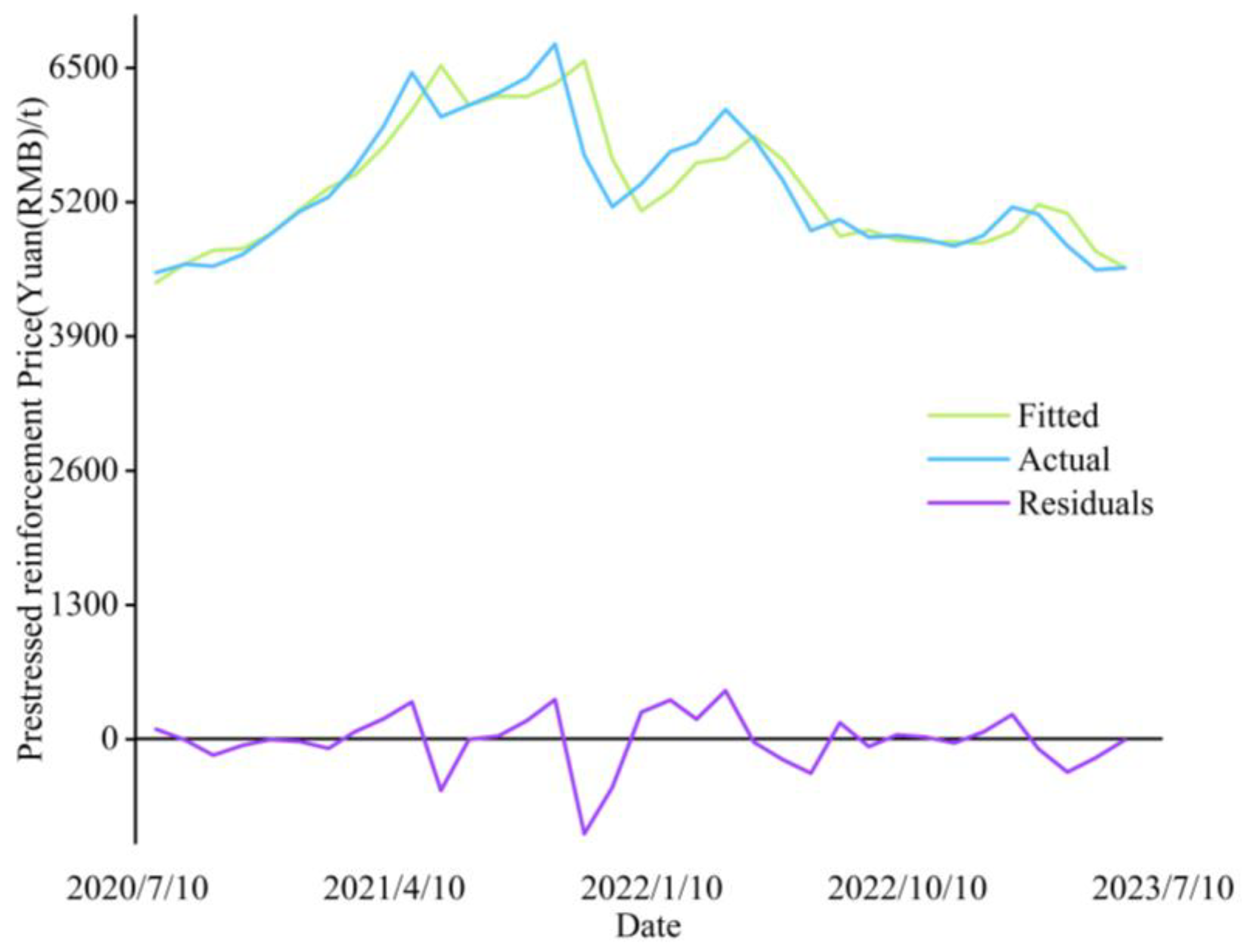
Figure 14.
Model evaluation result.
5. Discussion
The development of the CEEMDAN-VMD-GRU-ARIMA model represents a significant methodological advancement in price forecasting for construction materials, particularly PSB. By integrating complementary analytical paradigms—CEEMDAN and VMD for non-stationary signal decomposition, GRU for capturing temporal dependencies, and ARIMA for modeling linear trends—the hybrid framework addresses critical limitations in conventional single-model approaches. This dual quantitative-qualitative architecture demonstrates superior adaptability to market volatility, a persistent challenge in construction material pricing where external economic factors and supply-demand imbalances often induce nonlinear price fluctuations. The model’s self-optimizing capabilities, enabled by iterative learning mechanisms, offer a critical advantage in dynamic markets. Unlike static models requiring frequent recalibration, its adaptive structure aligns with the construction industry’s need for real-time decision support, particularly given that material costs account for 60-70% of total project expenditures. By reducing prediction errors through multi-scale feature extraction and hybrid learning, the framework enhances risk assessment accuracy for contractors and project managers, directly supporting cost containment strategies and tender pricing optimization. However, the current methodology focuses exclusively on historical price series, omitting exogenous variables such as raw material availability, policy changes, or geopolitical influences. While this ensures computational efficiency, it may limit predictive robustness during systemic market shocks a limitation partially mitigated by the model’s decomposition-recomposition mechanism but warranting further investigation. Practically, the framework’s success in PSB forecasting suggests transferability to other price-volatile construction materials, though domain-specific adjustments would be necessary. The theoretical contribution lies in demonstrating how hybrid architectures can reconcile econometric rigor with machine learning flexibility a paradigm applicable beyond construction to energy, agriculture, and financial markets.
Future extensions should prioritize three dimensionsincorporating macroeconomic indicators as model inputs,testing cross-market generalizability through comparative studies, anddeveloping real-time updating protocols for operational deployment. Such advancements could transform the model from a predictive tool into a prescriptive system, enabling proactive supply chain adjustments and policy-responsive budgeting in the construction sector.
6. Conclusion
This study presents the CEEMDAN-VMD-GRU-ARIMA model for PSB price forecasting, combining one-dimensional price series analysis with integrated machine learning and data mining techniques to generate precise and reliable predictions. The model's innovation lies in its dual analytical framework synthesizing quantitative and qualitative approaches, coupled with self-optimizing capabilities that enable dynamic market adaptation while preserving forecast validity. This hybrid architecture advances price prediction methodologies through its integration of adaptive learning mechanisms, offering both theoretical advancements and practical applications for market analytics and risk mitigation. Subsequent research will prioritize algorithmic refinement and extension to cross-market predictive applications.
Author Contributions
Conceptualization, Z.l.G. and X.n.J.; methodology, X.n.J.; software X.n.J.; validation, Z.l.G.; X.n.J.; Y.y.L. and T.q.Y.; investigation, X.n.J.; writing—original draft preparation, Z.l.G. and X.n.J.; writing—review and editing, Z.l.G.; X.n.J.; Y.y.L. and T.q.Y.; project administration, Z.l.G.; X.n.J. and J.M.; funding acquisition, Z.l.G. and X.n.J. All authors have read and agreed to the published version of the manuscript.
Funding
The grant was made with the financial support of the Natural Science Foundation of Anhui Provincial Education Department (2023AH053239) and Key Laboratory of Cryospheric Science and Frozen Soil Engineering, Chinese Academy of Sciences (KLCSFSE-ZZ-2025)
Data Availability Statement
The data presented in this study are available on request from the corresponding author.
Conflicts of Interest: The authors declare no conflict of interest.
References
- Wang, D.; Liu, J.; Wang, X.; Chen, Y. Cost-effectiveness analysis and evaluation of a ‘three-old’reconstruction project based on smart system. Cluster Computing 2019, 22, 7895–7905. [Google Scholar] [CrossRef]
- Hwang, S.; Park, M.; Lee, H.-S.; Kim, H. Automated time-series cost forecasting system for construction materials. Journal of construction engineering and management 2012, 138, 1259–1269. [Google Scholar] [CrossRef]
- Marzouk, M.; Hamdala, D. Phasing real estate projects considering profitability and customer satisfaction. Engineering, 2024. [Google Scholar]
- Musarat, M.A.; Alaloul, W.S.; Liew, M.; Maqsoom, A.; Qureshi, A.H. Investigating the impact of inflation on building materials prices in construction industry. Journal of Building Engineering 2020, 32, 101485. [Google Scholar] [CrossRef]
- Kissi, E.; Sadick, M.; Agyemang, D. Drivers militating against the pricing of sustainable construction materials: the Ghanaian quantity surveyors perspective. Case Stud Constr Mater 2018, 8, 507–516. [Google Scholar] [CrossRef]
- Zhao, C.; Hu, P.; Liu, X.; Lan, X.; Zhang, H. Stock market analysis using time series relational models for stock price prediction. Mathematics 2023, 11, 1130. [Google Scholar] [CrossRef]
- Guo, Z.; Jing, X.; Ling, Y.; Yang, Y.; Jing, N.; Yuan, R.; Liu, Y. Optimized air quality management based on air quality index prediction and air pollutants identification in representative cities in China. Scientific Reports 2024, 14, 17923. [Google Scholar] [CrossRef]
- Yin, Y.; Shang, P. Forecasting traffic time series with multivariate predicting method. Applied Mathematics and Computation 2016, 291, 266–278. [Google Scholar] [CrossRef]
- Mehrmolaei, S.; Savargiv, M.; Keyvanpour, M.R. Hybrid learning-oriented approaches for predicting Covid-19 time series data: A comparative analytical study. Engineering Applications of Artificial Intelligence 2023, 126, 106754. [Google Scholar] [CrossRef]
- Tarnate, W.R.D.; Ponci, F.; Monti, A. Uncertainty-aware model predictive control for residential buildings participating in intraday markets. IEEE Access 2022, 10, 7834–7851. [Google Scholar] [CrossRef]
- Uvarova, S.S.; Belyaeva, S.V.; Orlov, A.K.; Kankhva, V.S. Cost Forecasting for Building Materials under Conditions of Uncertainty: Methodology and Practice. Buildings 2023, 13, 2371. [Google Scholar] [CrossRef]
- Jiang, F.; Awaitey, J.; Xie, H. Analysis of construction cost and investment planning using time series data. Sustainability 2022, 14, 1703. [Google Scholar] [CrossRef]
- Ilbeigi, M.; Ashuri, B.; Joukar, A. Time-series analysis for forecasting asphalt-cement price. Journal of Management in Engineering 2017, 33, 04016030. [Google Scholar]
- Yin, L.; Wang, L.; Li, T.; Lu, S.; Tian, J.; Yin, Z.; Li, X.; Zheng, W. U-Net-LSTM: time series-enhanced lake boundary prediction model. Land 2023, 12, 1859. [Google Scholar] [CrossRef]
- Yuan, F.; Zhang, Z.; Fang, Z. An effective CNN and Transformer complementary network for medical image segmentation. Pattern Recognition 2023, 136, 109228. [Google Scholar]
- de Zarzà i Cubero, I.; de Curtò i Díaz, J.; Roig, G.; Calafate, C.T. LLM Multimodel Traffic Accident Forecasting. 2023. [Google Scholar]
- Tang, B.Q.; Han, J.; Guo, G.-f.; Chen, Y.; Zhang, S. Building material prices forecasting based on least square support vector machine and improved particle swarm optimization. Architectural Engineering and Design Management 2019, 15, 196–212. [Google Scholar]
- Mir, M.; Kabir, H.D.; Nasirzadeh, F.; Khosravi, A. Neural network-based interval forecasting of construction material prices. Journal of Building Engineering 2021, 39, 102288. [Google Scholar]
- Wang, J.; Ashuri, B. Predicting ENR construction cost index using machine-learning algorithms. International Journal of Construction Education and Research 2017, 13, 47–63. [Google Scholar]
- Liu, Y.; Qin, G.; Huang, X.; Wang, J.; Long, M. Autotimes: Autoregressive time series forecasters via large language models. arXiv preprint arXiv:2402.02370, arXiv:2402.02370 2024.
- Wang, Y.; Yang, D.; Liu, Y. A real-time look-ahead interpolation algorithm based on Akima curve fitting. International Journal of Machine Tools and Manufacture 2014, 85, 122–130. [Google Scholar]
- Hamilton, J.D. Why you should never use the Hodrick-Prescott filter. Review of Economics and Statistics 2018, 100, 831–843. [Google Scholar] [CrossRef]
- Nasir, J.; Aamir, M.; Haq, Z.U.; Khan, S.; Amin, M.Y.; Naeem, M. A new approach for forecasting crude oil prices based on stochastic and deterministic influences of LMD Using ARIMA and LSTM Models. IEEE Access 2023, 11, 14322–14339. [Google Scholar] [CrossRef]
- Jun, W.; Yuyan, L.; Lingyu, T.; Peng, G. A new weighted CEEMDAN-based prediction model: An experimental investigation of decomposition and non-decomposition approaches. Knowledge-based systems 2018, 160, 188–199. [Google Scholar]
- Gao, B.; Huang, X.; Shi, J.; Tai, Y.; Zhang, J. Hourly forecasting of solar irradiance based on CEEMDAN and multi-strategy CNN-LSTM neural networks. Renewable Energy 2020, 162, 1665–1683. [Google Scholar] [CrossRef]
- Shumway, R.H.; Stoffer, D.S. Time series analysis and its applications (springer texts in statistics); Springer-Verlag: 2005.
- Thiruchelvam, L.; Dass, S.C.; Asirvadam, V.S.; Daud, H.; Gill, B.S. Determine neighboring region spatial effect on dengue cases using ensemble ARIMA models. Scientific Reports 2021, 11, 5873. [Google Scholar]
- Gan, M.; Pan, H.; Chen, Y.; Pan, S. Application of the Variational Mode Decomposition (VMD) method to river tides. Estuarine, Coastal and Shelf Science 2021, 261, 107570. [Google Scholar]
- Li, X.P.; Shi, Z.-L.; Leung, C.-S.; So, H.C. Sparse index tracking with K-sparsity or ϵ-deviation constraint via ℓ 0-norm minimization. IEEE Transactions on Neural Networks and Learning Systems 2022, 34, 10930–10943. [Google Scholar]
- Nazari, M.; Sakhaei, S.M. Successive variational mode decomposition. Signal Processing 2020, 174, 107610. [Google Scholar]
- Wang, M.-H.; Hung, C. Extension neural network and its applications. Neural Networks 2003, 16, 779–784. [Google Scholar]
- Hu, C.; Cheng, F.; Ma, L.; Li, B. State of charge estimation for lithium-ion batteries based on TCN-LSTM neural networks. Journal of the Electrochemical Society 2022, 169, 030544. [Google Scholar]
- Ghazvini, A.; Sharef, N.M.; Sidi, F.B. Prediction of Course Grades in Computer Science Higher Education Program Via a Combination of Loss Functions in LSTM Model. IEEE Access 2024. [Google Scholar]
- Gao, S.; Huang, Y.; Zhang, S.; Han, J.; Wang, G.; Zhang, M.; Lin, Q. Short-term runoff prediction with GRU and LSTM networks without requiring time step optimization during sample generation. Journal of Hydrology 2020, 589, 125188. [Google Scholar]
- Xu, M.; Shang, P.; Lin, A. Cross-correlation analysis of stock markets using EMD and EEMD. Physica A: Statistical Mechanics and its Applications 2016, 442, 82–90. [Google Scholar]
- Huang, Y.; Yu, J.; Dai, X.; Huang, Z.; Li, Y. Air-quality prediction based on the EMD–IPSO–LSTM combination model. Sustainability 2022, 14, 4889. [Google Scholar] [CrossRef]
- Dong, H.; Qi, K.; Chen, X.; Zi, Y.; He, Z.; Li, B. Sifting process of EMD and its application in rolling element bearing fault diagnosis. Journal of mechanical science and technology 2009, 23, 2000–2007. [Google Scholar]
- Ding, J.; Xiao, D.; Huang, L.; Li, X. Gear fault diagnosis based on VMD sample entropy and discrete hopfield neural network. Mathematical Problems in Engineering 2020, 2020, 8882653. [Google Scholar]
- Zhang, P.; Gao, D.; Lu, Y.; Kong, L.; Ma, Z. Online chatter detection in milling process based on fast iterative VMD and energy ratio difference. Measurement 2022, 194, 111060. [Google Scholar]
- Wang, Y.; Chen, P.; Zhao, Y.; Sun, Y. A denoising method for mining cable PD signal based on genetic algorithm optimization of VMD and wavelet threshold. Sensors 2022, 22, 9386. [Google Scholar] [CrossRef]
- Wang, H.; Wu, F.; Zhang, L. Application of variational mode decomposition optimized with improved whale optimization algorithm in bearing failure diagnosis. Alexandria Engineering Journal 2021, 60, 4689–4699. [Google Scholar]
- Li, J.; Yao, X.; Wang, H.; Zhang, J. Periodic impulses extraction based on improved adaptive VMD and sparse code shrinkage denoising and its application in rotating machinery fault diagnosis. Mechanical Systems and Signal Processing 2019, 126, 568–589. [Google Scholar]
Figure 1.
The chart of the PSB box type.
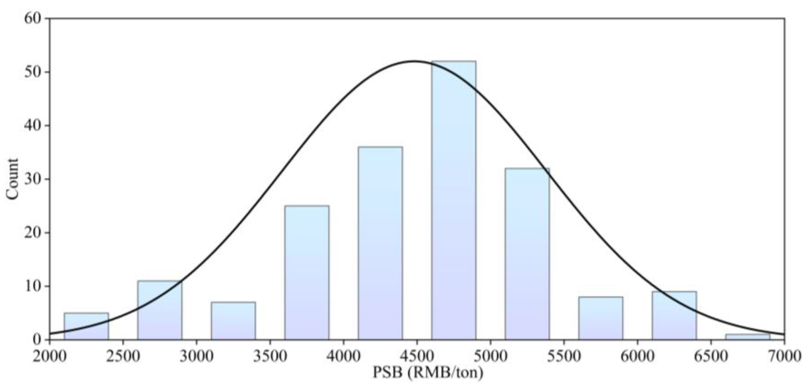
Figure 2.
Analysis results of PSB with Hodrick-Prescott filter.
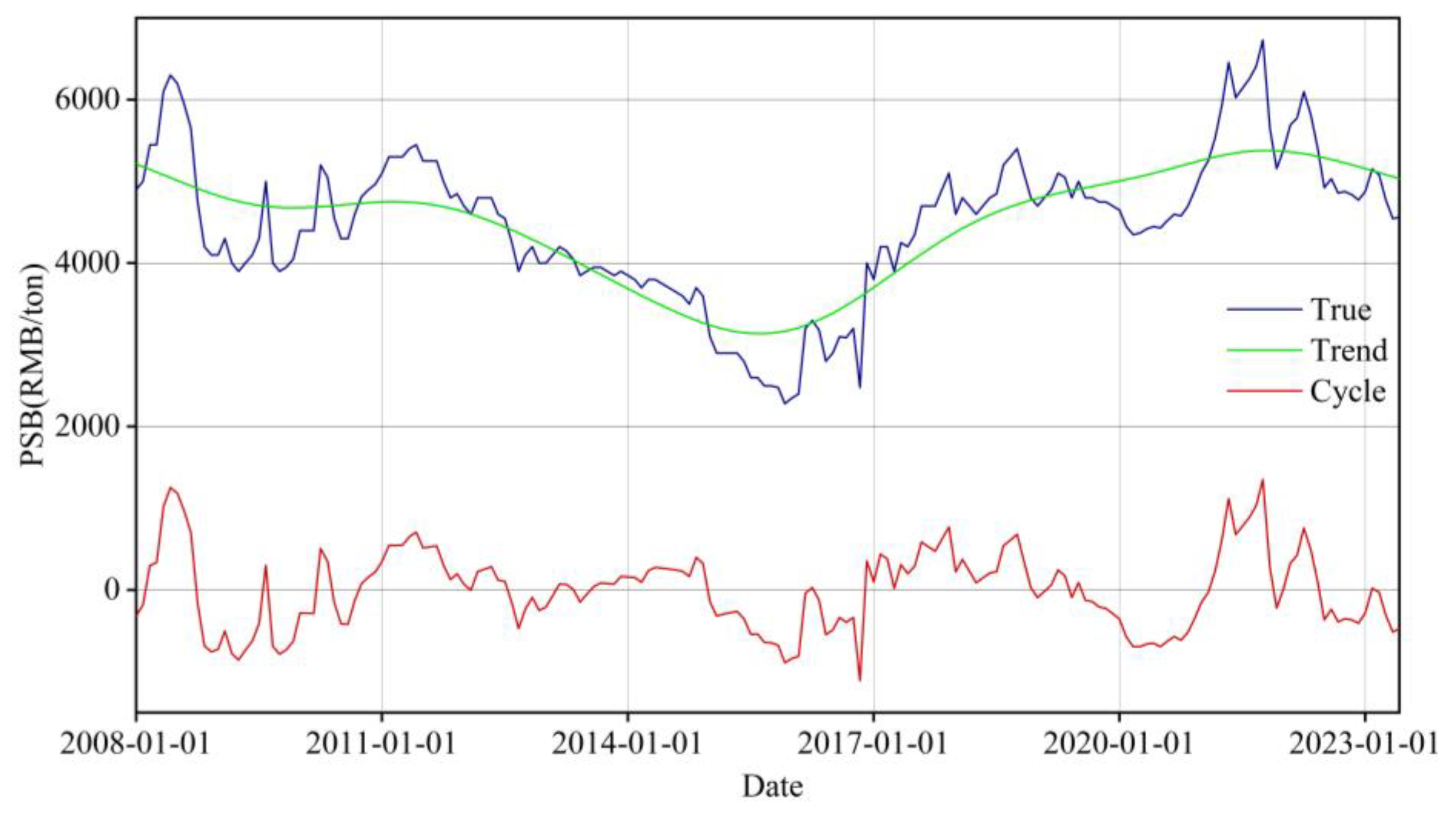
Figure 3.
Research Framework Structure.
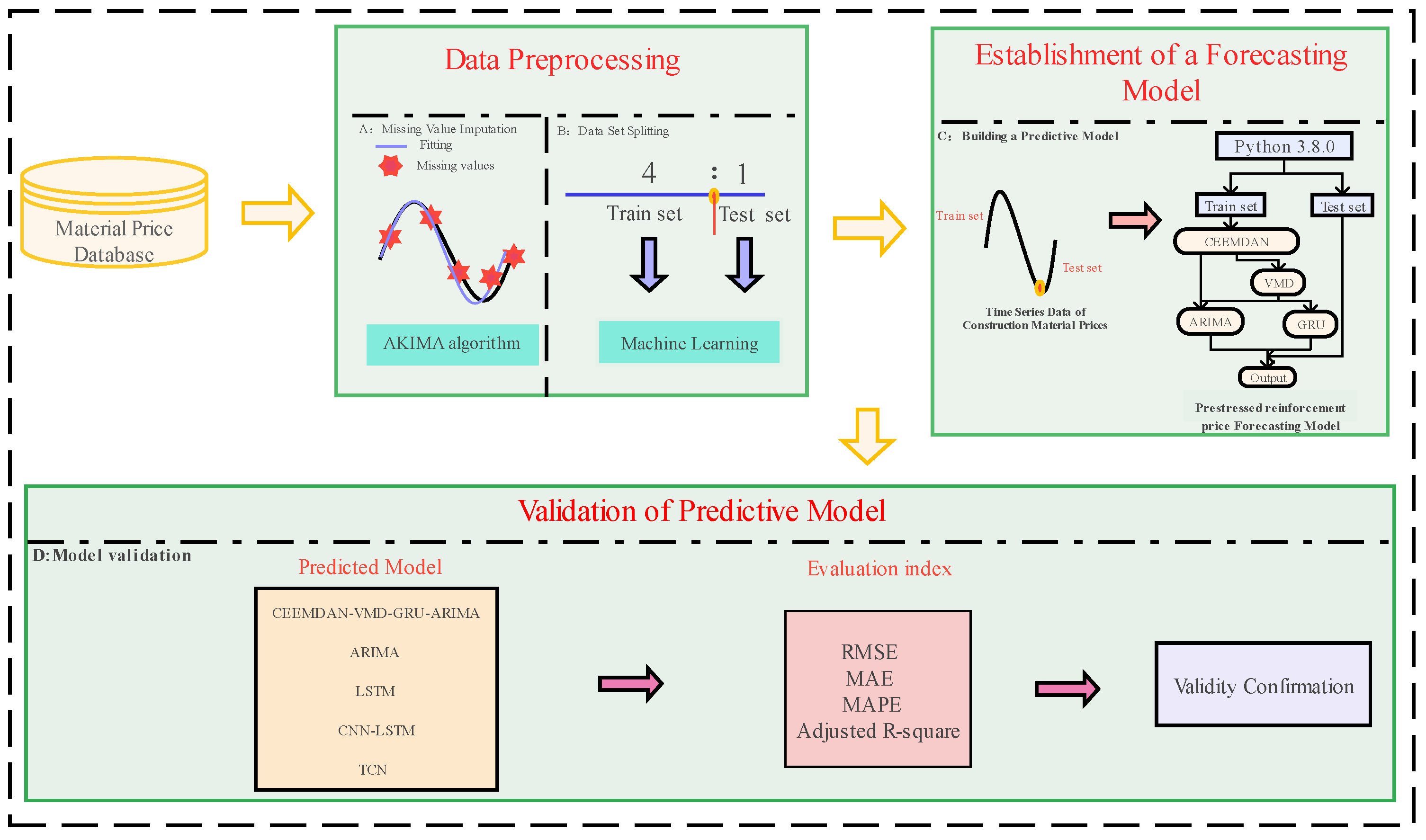
Figure 5.
The structure chart for the price forecast of PSB.
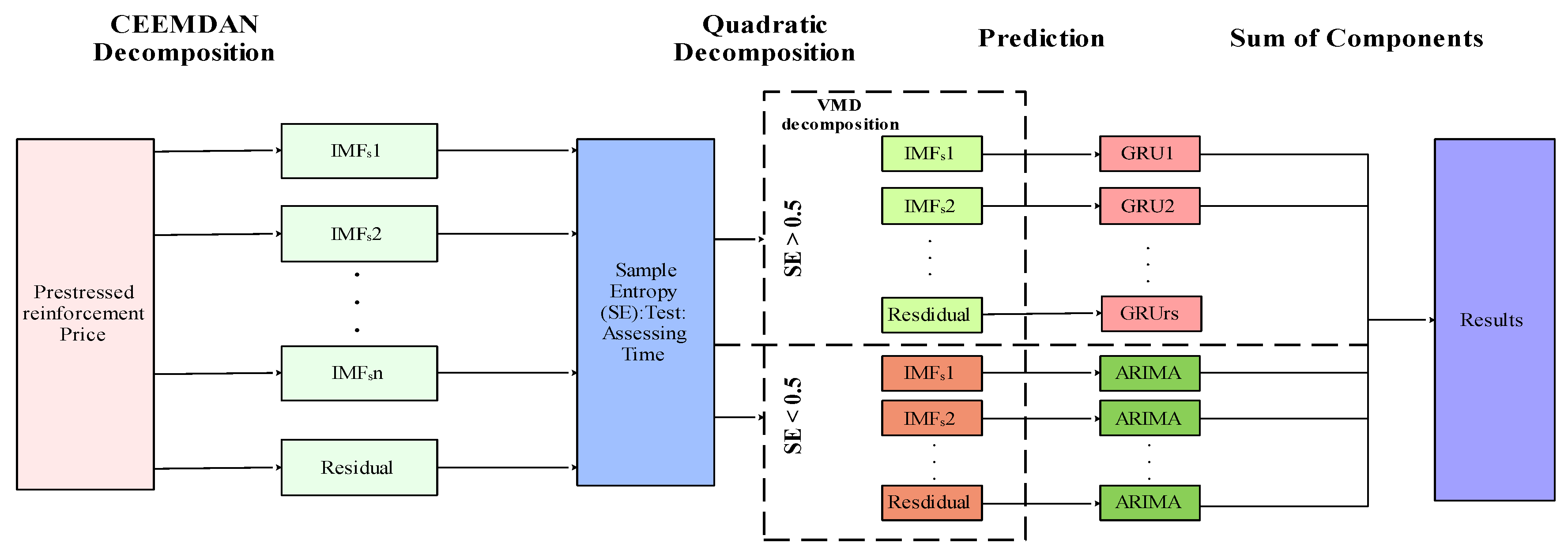
Figure 6.
Results of CEEMDAN Decomposition.
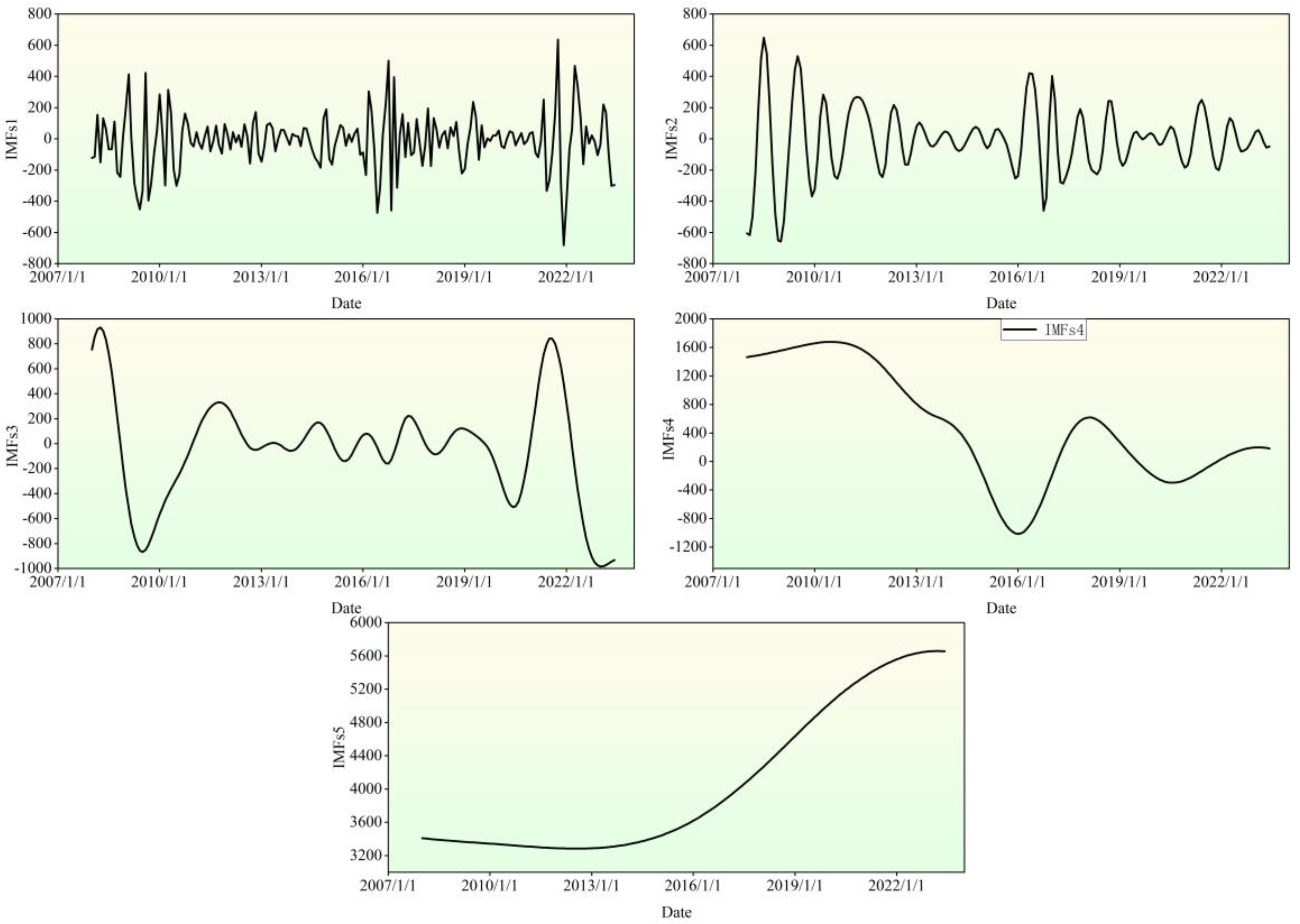
Figure 7.
Sample entropy of each component for simulation analysis.
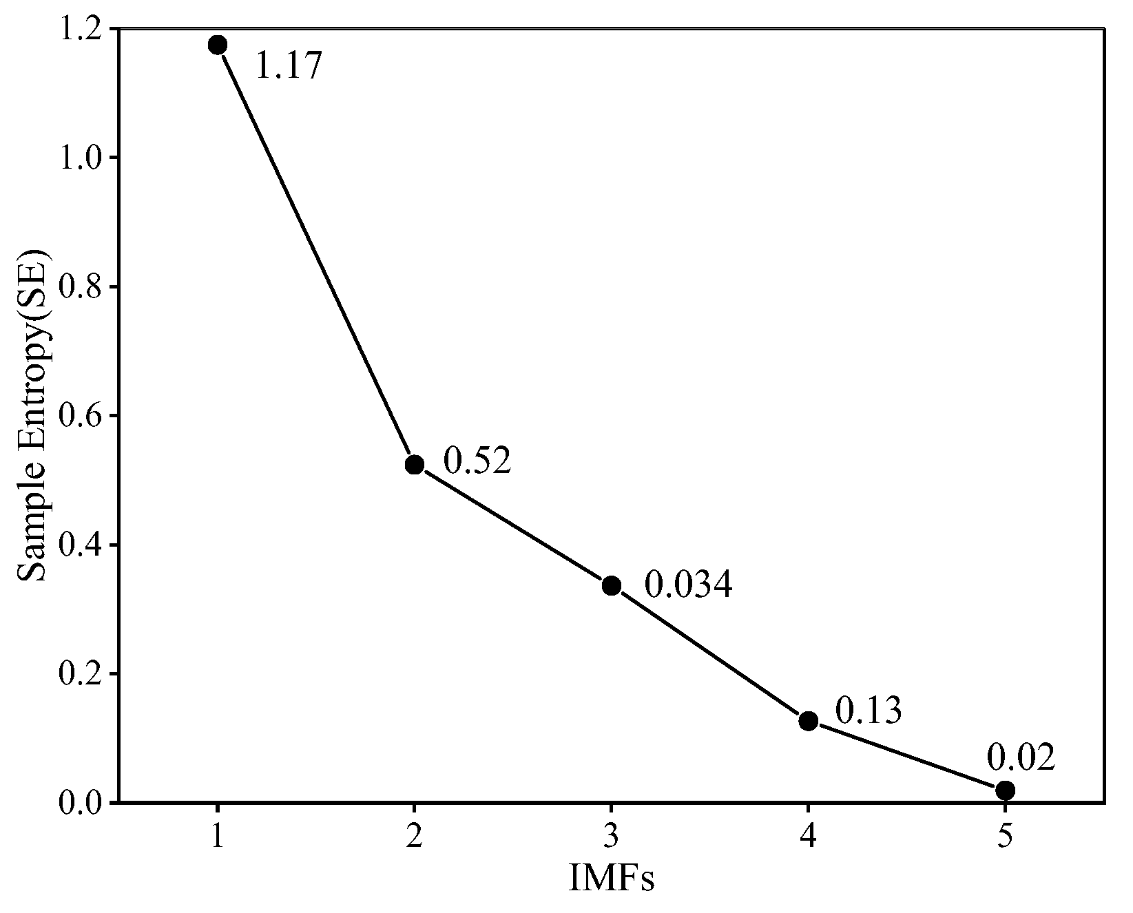
Figure 8.
K-Valued Optimization Solution for VMD Decomposition of IMF.
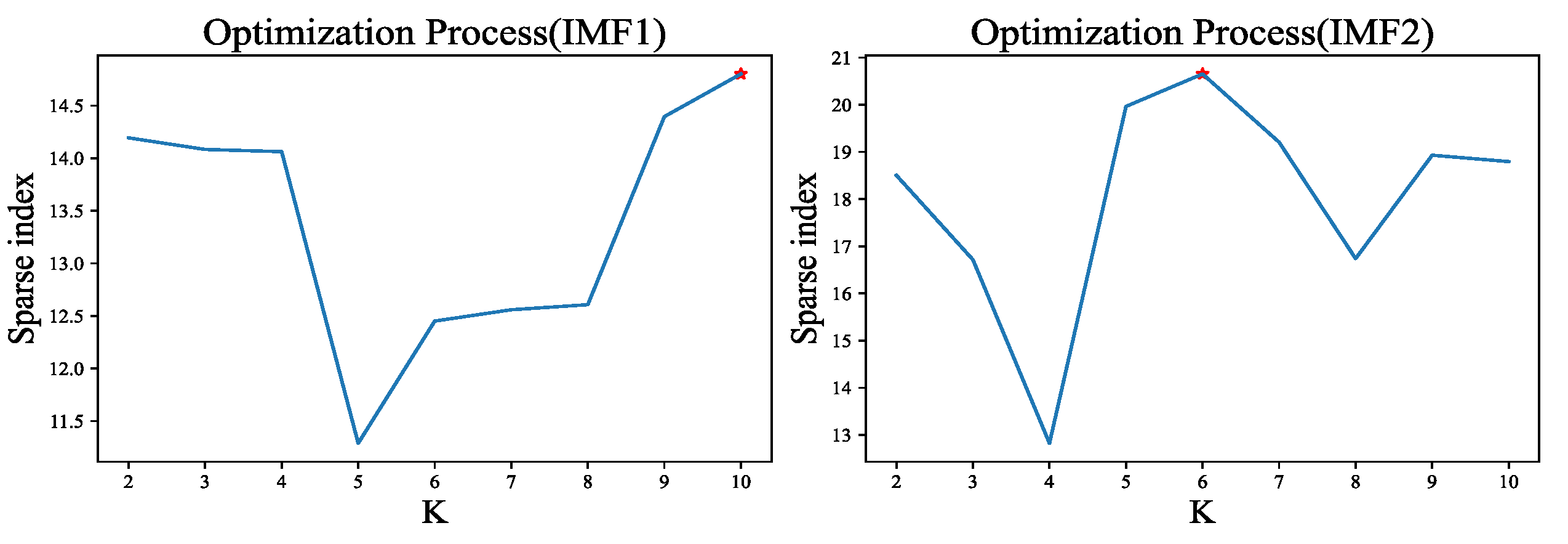
Figure 10.
CEEMDAN-VMD Decomposition Results: Modal Feature Analysis of Variable IMF1s.
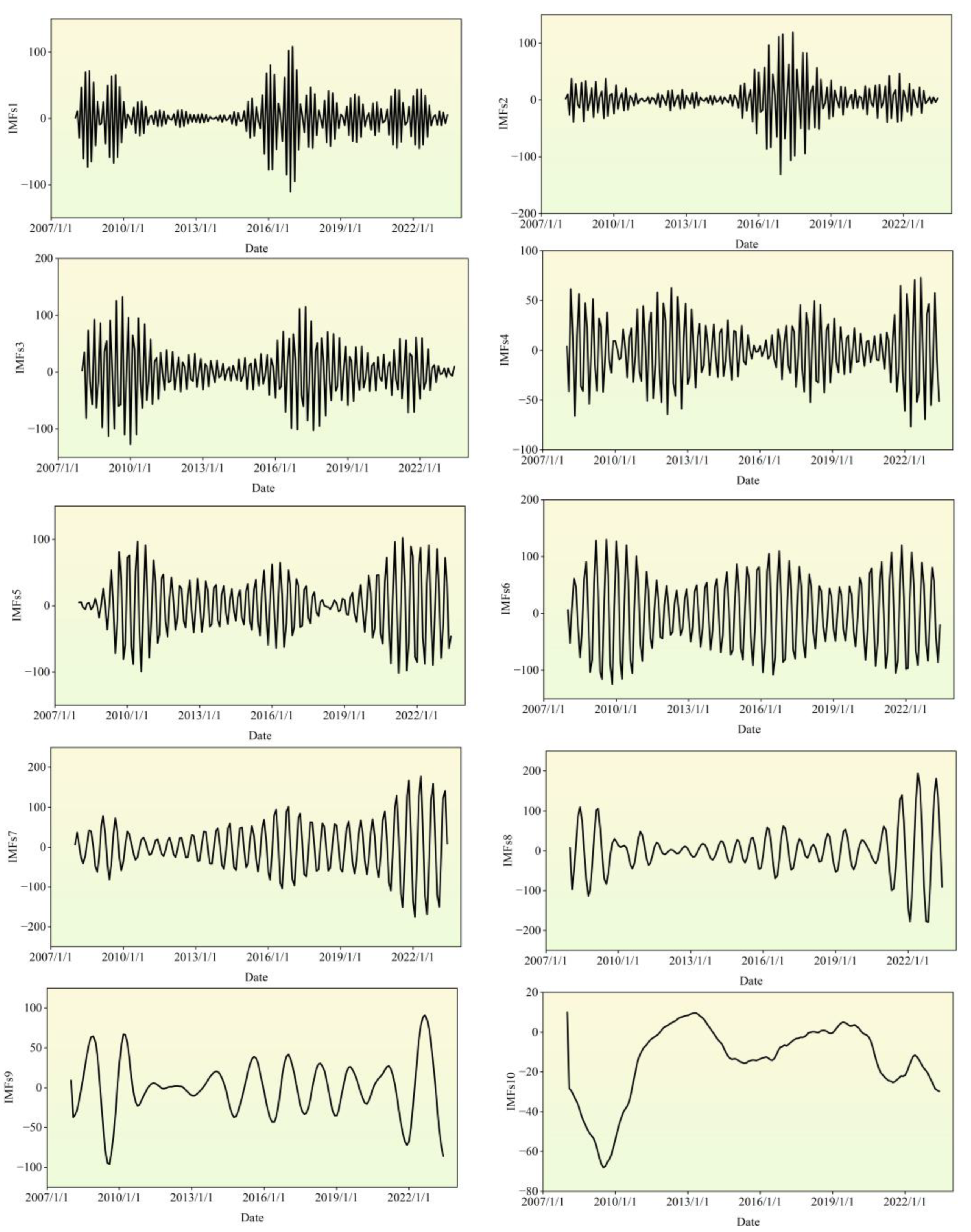
Figure 11.
CEEMDAN-VMD Decomposition Results: Modal Feature Analysis of Variable IMF2s.
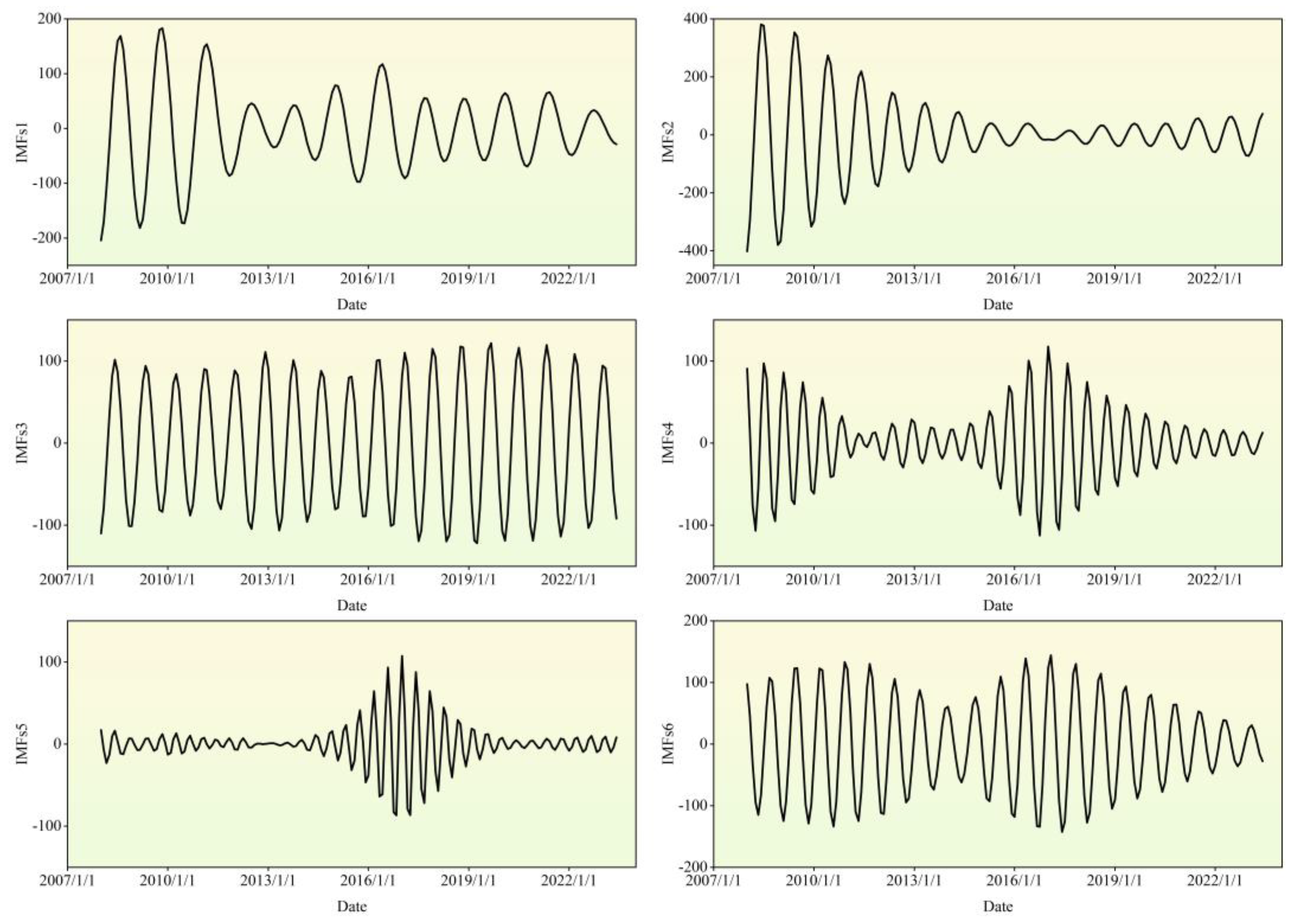
Figure 12.
The marginal histogram of Actual and Fitted values of PSB.
Disclaimer/Publisher’s Note: The statements, opinions and data contained in all publications are solely those of the individual author(s) and contributor(s) and not of MDPI and/or the editor(s). MDPI and/or the editor(s) disclaim responsibility for any injury to people or property resulting from any ideas, methods, instructions or products referred to in the content. |
© 2025 by the authors. Licensee MDPI, Basel, Switzerland. This article is an open access article distributed under the terms and conditions of the Creative Commons Attribution (CC BY) license (http://creativecommons.org/licenses/by/4.0/).
Copyright: This open access article is published under a Creative Commons CC BY 4.0 license, which permit the free download, distribution, and reuse, provided that the author and preprint are cited in any reuse.


