Submitted:
18 February 2025
Posted:
18 February 2025
You are already at the latest version
Abstract
In order to meet the requirements of higher economic operating speed, constructing a vacuum tube operating environment is an important direction for the future development of ultra high speed rail transit technology. Due to the non-stationary nature of wireless channels during ultra high speed movement, traditional wireless channel models are no longer suitable for ultra high speed train communication systems in vacuum tube scenarios. Existing channel modeling methods cannot accurately reflect the wave propagation characteristics. This article is based on the GBSM (Geometry based Stochastic Model) modeling method, which abstracts it as a two sphere geometric model from the actual scene and simulates the vehicle ground wireless channel model. In the model, obstacles encountered on the propagation path of waves are fitted into effective scatterers randomly distributed on the surface of a geometric object. The space-time correlation function (STCF), cross correlation function (CCF), and auto correlation function (ACF) of the model are derived to analyze the time-varying characteristics of the channel. The experimental results indicate that LOS components and Doppler effects have an impact on the channel characteristics of the entire system. This provides theoretical and technical support for the wireless communication system of the vacuum tube maglev system.
Keywords:
vacuum tube
; wireless channel
; time-varying characteristics
; GBSM modeling
1. Introduction
With the vigorous development of rail transit technology, wireless communication technology in vacuum tube environments has also been studied in recent years. However, due to the special of vacuum systems, their electromagnetic signals propagate in confined and enclosed spaces. If the vacuum tube maglev system uses traditional wireless free wave access, the wireless link between the base station outside the vacuum pipeline and the passengers inside the carriage will undergo two major penetration fading (metal pipeline and vehicle body), resulting in a sharp decrease in the signal-to-noise ratio of the receiving end signal. Therefore, the traditional wireless access method is not suitable for the operation of the vacuum tube maglev system. The use of leaky wave system for vehicle ground communication is currently a suitable and feasible approach [1]. The leaky wave system is used for coupled transmission, and the leaky wave structure is installed at the top of the vacuum tube, with its coverage field diffusing and radiating inside the metal cavity. To provide a more reliable theoretical basis for the design of communication systems in vacuum tube scenarios, it is necessary to establish a MIMO channel model for vacuum tube scenarios and study its time-varying characteristics.
Millimeter wave communication systems have the characteristics of large communication capacity, good security and confidentiality, high transmission quality, and all-weather communication [2]. They can provide highly reliable and low latency data transmission during high-speed train operation. So currently, 38GHz millimeter wave is used as the communication frequency for the vehicle ground communication system.
The most commonly used channel model currently is the Geometry based Stochastic Model (GBSM), which is based on geometric distribution. The propagation characteristics of waves mainly depend on the distribution of scatterers in the channel environment. In order to maintain ease of processing, it can be assumed that the effective scatterers of GBSM are all located on regular shapes [3]. Reference [4] proposes a single reflection channel model based on geometric distribution, which describes a non frequency selective Rayleigh fading channel model but only considers a single reflection path. Reference [5] introduces a vertical dimension on this basis and proposes a 3D massive MIMO GBSM model, studying the spatiotemporal correlation function and influencing factors of the model. Reference [6] proposes a double sphere model, in which scattered objects such as walls and floors are randomly distributed on a spherical surface surrounding the transmitting and receiving antennas in a closed indoor scene. In this 3D model, both the transmitting and receiving antennas are fixed and the mobility of the antennas is not considered.
Based on the particularity of vacuum tube scenarios (closed characteristics), this paper introduces the high-speed mobility of trains and the height difference of transmitting and receiving antennas on the basis of [6], proposes a MIMO GBSM channel model suitable for vacuum tube scenarios, and studies the time-varying characteristics of the model, providing theoretical and technical support for the wireless communication system of vacuum tube maglev trains.
2. Materials and Methods
2.1. System Model
The vacuum tube scenario is different from the normal train operation scenario. In order to meet the requirements of higher speed operation, maglev trains travel at ultra-high speeds in low mechanical friction, low air resistance, and low noise mode inside the vacuum tube, with a speed of up to 1000km/h. Therefore, higher requirements are placed on the communication stability and reliability between the train and the ground [7]. But its mobile communication system environment is limited to a fixed metal cavity. When electromagnetic waves propagate in tubes, in addition to direct radiation, they are also reflected by tube walls and vehicle bodies. The physical structure and communication method of the vacuum tube scene, as shown in Figure 1, is a closed environment. The leaky wave structure is installed at the top of the vacuum tube, and the receiving end is on the ultra high speed maglev train. The communication channel between the two is confined in a limited space.
Because dipole antennas can form omnidirectional radiation, dipole antennas are used as transmitting and receiving antennas to study their radiation patterns, and the dipole antenna is placed in a steel material pipeline to study the changes in its radiation pattern. The radiation pattern is as follows Figure 2.
All obstacles (scatterers) in the wireless communication environment are located within an approximately spherical area centered around the transmitting antenna, and the propagation environment is the radiation coverage area of the omnidirectional antenna. Based on a certain statistical distribution, the wireless mobile communication system is simplified into a mobile communication system with MT transmitting antennas and MR receiving antennas. In the case of a wide propagation range, the height difference between the transmitting and receiving antennas can be ignored. However, in the narrow space of the vacuum pipeline maglev system, the height difference between the transmitting and receiving antennas cannot be ignored. The 3D MIMO GBSM in the established vacuum pipeline scene is shown in Figure 3, and its parameters are listed in Table 1.
2.2. Model Calculation Method
The number of antennas at the transmitting end and at the receiving end can be extended to any number, with and being the -th antenna at the transmitting end and the -th antenna at the receiving end, respectively. The sequence number of the antenna satisfies , . Multiple reflections can be seen as a combination of single and double reflections. In order to reduce the complexity of GBSM, only the line of sight path LOS, single hop path, and double hop path are considered. In this model, the antenna at the transmitting end is referred to as , and the antenna at the receiving end is referred to as . There are effective scatterers such as maglev train bodies and pipeline walls near . There are effective scatterers such as the maglev train body and pipeline walls near . Assuming effective scatterers are randomly distributed on a spherical surface with as the center and as the radius, the th scatterer is denoted as . Similarly, effective scatterers are randomly distributed on a spherical surface with as the center and as the radius, and the th scatterer is denoted as . A cylinder with radius is used to simulate the effective scatterers of the tube wall, with effective scatterers, and the th scatterer. The scatterer is denoted as .
The MIMO fading channel can be represented by a matrix in the dimension, where is the time-varying channel impulse response between the -th transmitting antenna and the -th receiving antenna, and can be expressed as the superposition of LoS, SB, and DB components. That is
Among them, the LoS component, SB component, and DB component are respectively represented as,
is the Rayleigh factor of the channel; is the total power of the channel;, , , are the power correlation coefficient,there are ; is the wavelength of electromagnetic waves.
Calculate the distance among them:
The distance between antenna and antenna :
The distance between antenna and antenna :
The distance between antenna and scatterer :
The distance between antenna and scatterer :
The distance between antenna and scatterer :
The distance between antenna and scatterer :
The distance between antenna and scatterer :
The distance between antenna and scatterer :
The distance between antenna and scatterer :
The distance between antenna and scatterer :
The distance between antenna and scatterer :
The distance between antenna and scatterer :
The distance between antenna and scatterer :
The distance between antenna and scatterer :
The distance between the center of the sender's circle and the scatterer :
The distance between the center of the sender's circle and the scatterer :
The distance between the center of the receiving end and the scatterer :
The distance between the center of the receiving end and the scatterer :
2.3. Statistical Characteristics of System Models
In order to more effectively evaluate the performance of MIMO GBSM in vacuum tube environments, it is necessary to analyze the spatial and temporal correlations as well as statistical characteristics such as Doppler of MIMO channels.
2.3.1. Space Time Correlation Function
STCT reflects the correlation between any two antenna elements in the geometric channel model inside a vacuum tube in space and time. The spatiotemporal correlation function of any two sub channels and can be expressed as:
represents mathematical expectation operation; * Representing complex conjugate operations.
Due to the independence of the LoS component and the SB and DB components of the near and far scatterers.
The above equation can be expressed as the sum of STCFs with different components:
Among them, the LOS part can be defined as:
The SB part can be defined as:
Just: , , ;
The DB part can be defined as:
Just: , , ;
2.3.2. Time Autocorrelation Function
The time autocorrelation function reflects the impact of multipath effects inside the pipeline from a temporal perspective, reflecting the correlation between signals arriving at the receiving end through different paths. By setting in STCT, its expression can be derived.
2.3.3. Spatial Cross-Correlation Function
The spatial cross-correlation function studies the impact of the correlation between different antenna elements on channel performance from a spatial perspective. When the antenna spacing is too small, it can cause channel fading and result in errors. So CCF is also the key to reflecting the internal channel performance of pipelines. If in the previous STCT, its expression can be obtained.
2.3.4. Doppler Power Spectral Density
The movement speed of the ultra high speed train inside the vacuum tube causes Doppler frequency deviation, which affects the channel performance.
DPSD can be obtained by Fourier transform of the time-dependent function ACF, and the specific expression is:
However, due to the different Doppler shifts of the LoS, SB, and DB paths, it is necessary to first calculate the ACF and Doppler frequencies of the three paths to obtain the DPSD of the LoS, SB, and DB paths, and then composite and stack them.
3. Results and Discussion
By analyzing the scattering path of the random geometric model of the vacuum pipeline maglev system and mathematically deriving its geometric relationship, the expressions of STCT, ACF, CCF, and DPSD for the reference model and simulation model of the entire system were obtained. However, it is difficult to intuitively see the trend of the autocorrelation function over time or space solely based on mathematical formulas. Therefore, in this study, MATLAB was used to simulate the obtained mathematical model.
Based on the channel model proposed in this article, statistical characteristics analysis was conducted, and the selected parameters are shown in Table 2:
As shown in Figure 4, when a certain specific value is taken, the change of has almost no effect on the value of CCF. And when a certain value is taken, the change in has almost no effect on the value of CCF. This means that the elevation angle of the transmitting and receiving antenna elements has almost no effect on the spatial correlation of the channel.
As shown in Figure 5, the purple solid line is the simulation model, and the green solid line is the reference model. There is a steep downhill trend as the distance between the rceiving antennas increases, followed by a slight fluctuation as the distance between the receiving antennas increases. This indicates that the presence of LOS components will have a certain impact on CCF, causing it to fluctuate. And the curve trends of the simulation model and the reference model are roughly the same, which also verifies the correctness of the simulation model.
Figure 6 shows the temporal variation of Doppler power spectrum at different speeds. It can be seen from the figure that when v=1000km/h, the Doppler power spectrum is most concentrated and has the highest value. When the speed increases to 1400km/h, the energy relatively decreases. When the speed decreases to 600km/h, the power spectrum disperses into two clusters and the energy is no longer concentrated in one place. This indicates that the speed variation of trains in the pipeline will affect the channel performance.
The definition of the Rayleigh factor K is the ratio of the variance of the LOS path signal to the multipath signal, which represents the proportion of LOS in the signal. The larger the value of K, the greater the proportion of LOS. So this simulation investigates the impact of LOS components on channel correlation by varying the K value. Simulations were conducted on the temporal and spatial correlations at K=1, 5, 10, and 20 in the figure. From the Figure 7, it can be seen that the larger the Rice factor, the higher the curves of ACF and CCF, so the more LOS components there are, the greater the autocorrelation performance of the channel, and as the K value continues to increase, the interval between the curves shortens, indicating that this influence is somewhat limited.
4. Conclusions
This paper proposes a double sphere stochastic geometry model for the communication system of ultra high speed trains in vacuum tube scenarios. By introducing different parameters such as train speed and height difference of transmitting and receiving antennas, the channel characteristics of STCF, DPSD, etc. are analyzed in detail. Considering the complexity of the algorithm, the model only considers three paths: LOS, SB, and DB. Through geometric analysis, the STCF, ACF, CCF, and DPSD of the three paths are derived and simulated using MATLAB. The simulation results show that the Doppler effect has an undeniable impact on channel performance, and the larger the K value, the greater the impact of LOS component on channel performance. Provide theoretical and technical support for the wireless communication system of vacuum tube maglev train.
References
- J. Zhang et al., "Two Novel Structures of Broadband Wireless Communication for High-speed Flying Train in Vacuum Tube," 2019 28th Wireless and Optical Communications Conference (WOCC), Beijing, China, 2019, pp. 1-5. [CrossRef]
- 卫慧. 磁浮交通车地通信系统毫米波传输特性的研究[D]. 上海:上海大学,2010.
- Zheng, K,Yin, X F. Massive MIMO channel models: A survey[J]. International Journal of Antennas and Propagation,2014,2014(11):1-10.
- H. -d. Zheng and X. -y. Nie, "GBSB Model for MIMO Channel and Its Space-Time Correlataion Analysis in Tunnel," 2009 International Conference on Networks Security, Wireless Communications and Trusted Computing, Wuhan, China, 2009, pp. 8-11. [CrossRef]
- 蒋育康,郭爱煌,艾渤,等.城市轨道交通隧道环境下大规模MIMO信道建模[J].铁道学报,2018,40(11):84-90.
- WANG F, CHENG X, YANG L. On the achievable capacity of dual-polarized antenna systems in 3D indoor scenarios[C]. CIC International Conference on Communications in China (ICCC).IEEE.2013: 2377-8644.
- 徐飞,罗世辉,邓自刚.磁悬浮轨道交通关键技术及全速度域应用研究[J].铁道学报,2019,41(03):40-49.
Figure 1.
Schematic diagram of vacuum tube communication scenario.
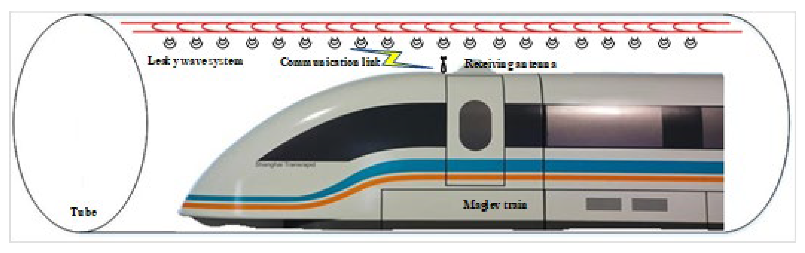
Figure 2.
Radiation pattern. (a) Radiation pattern of dipole antenna; (b) Radiation pattern of dipole antenna in metal tube.
Figure 2.
Radiation pattern. (a) Radiation pattern of dipole antenna; (b) Radiation pattern of dipole antenna in metal tube.
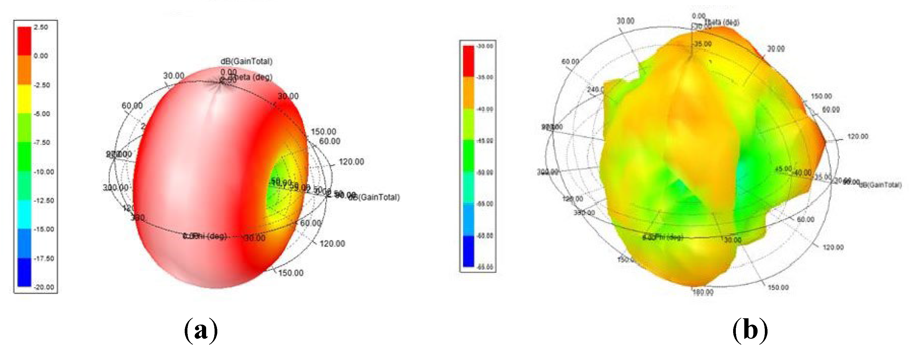
Figure 3.
3D MIMO GBSM in vacuum tube scene.
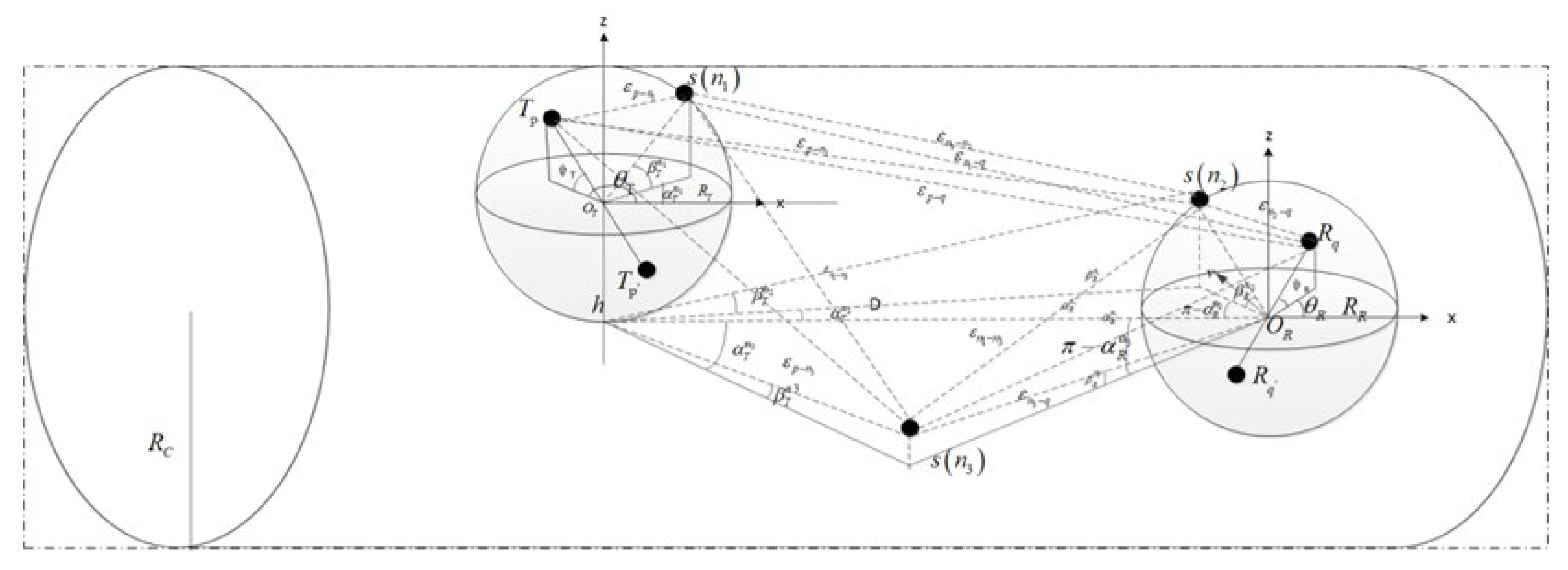
Figure 4.
The influence of the elevation angle of the transmitting and receiving antennas on CCF.
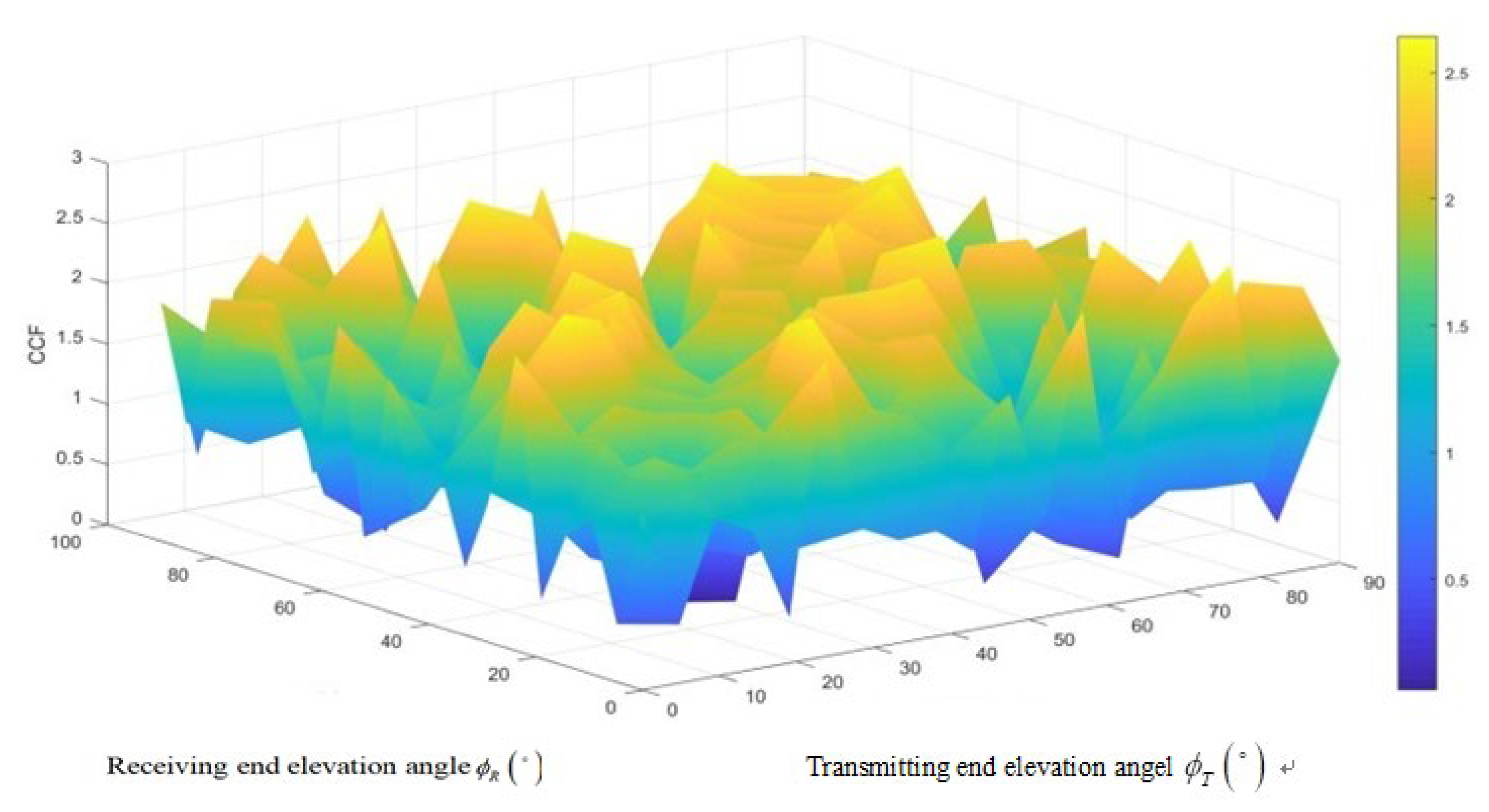
Figure 5.
Trend chart of CCF variation with receiving antenna spacing.
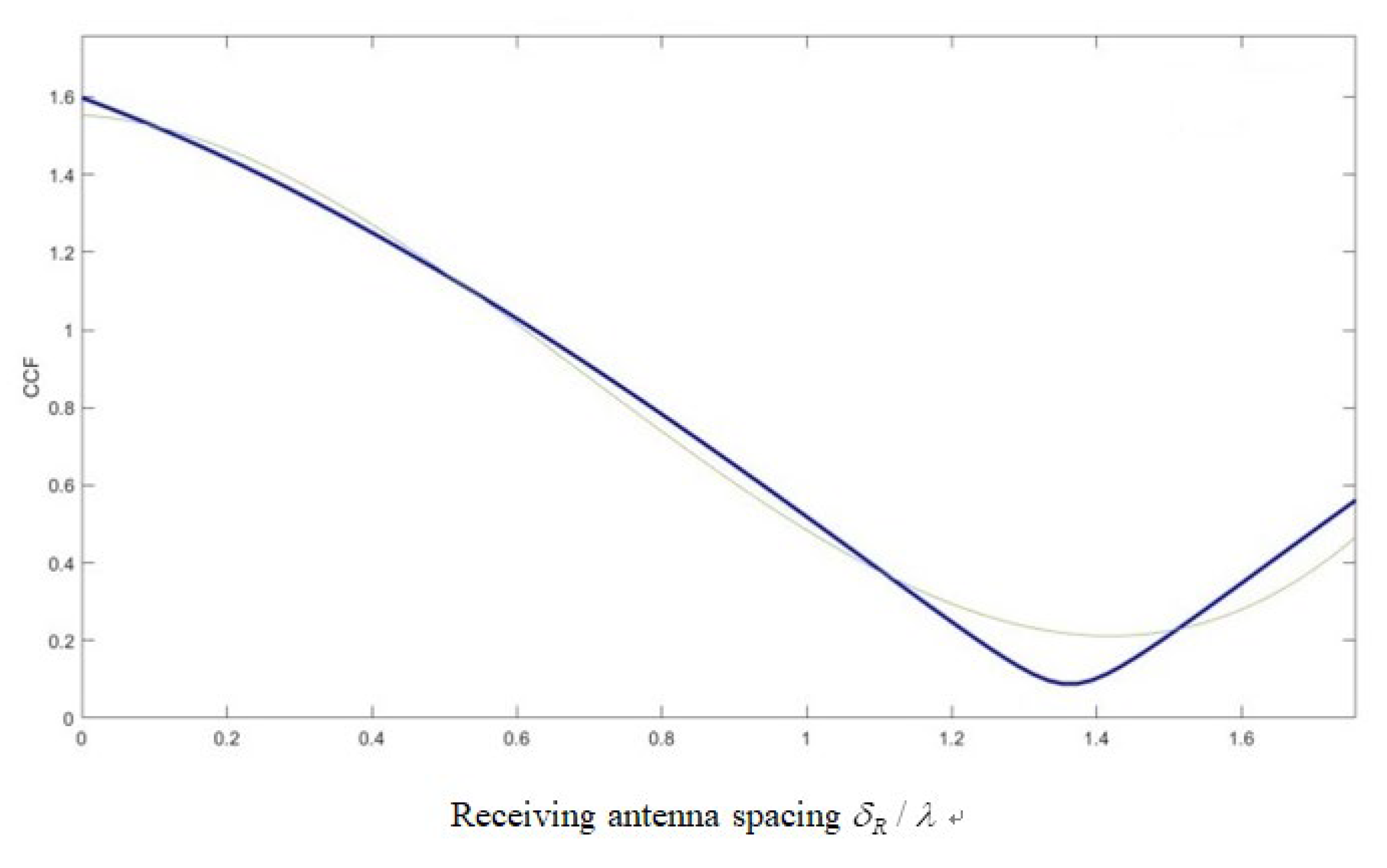
Figure 6.
DPSD versus velocity variation graph.
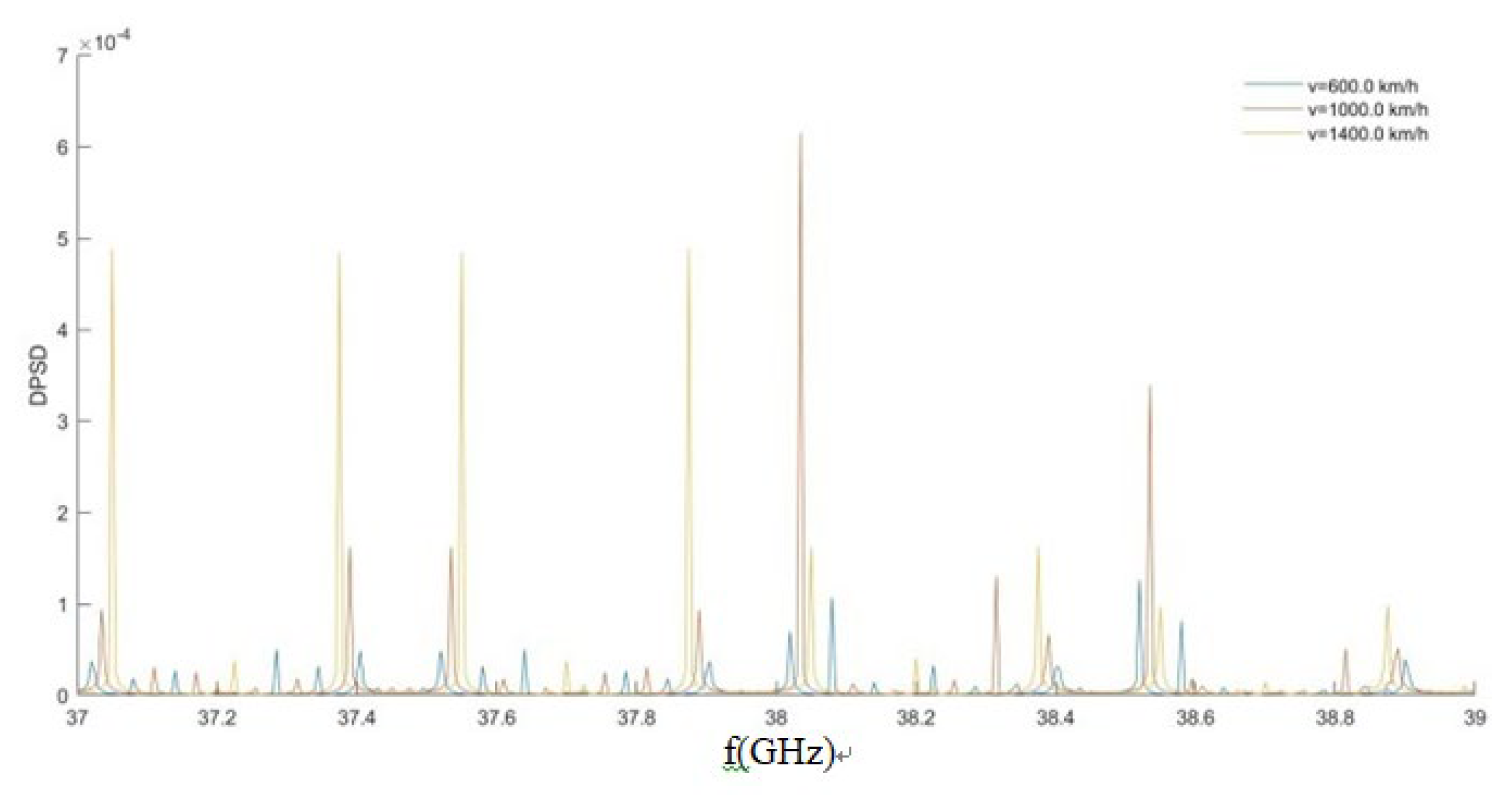
Figure 7.
(a)CCF versus Rice Factor Variation Chart;.(b) ACF versus Rice Factor Variation Chart.
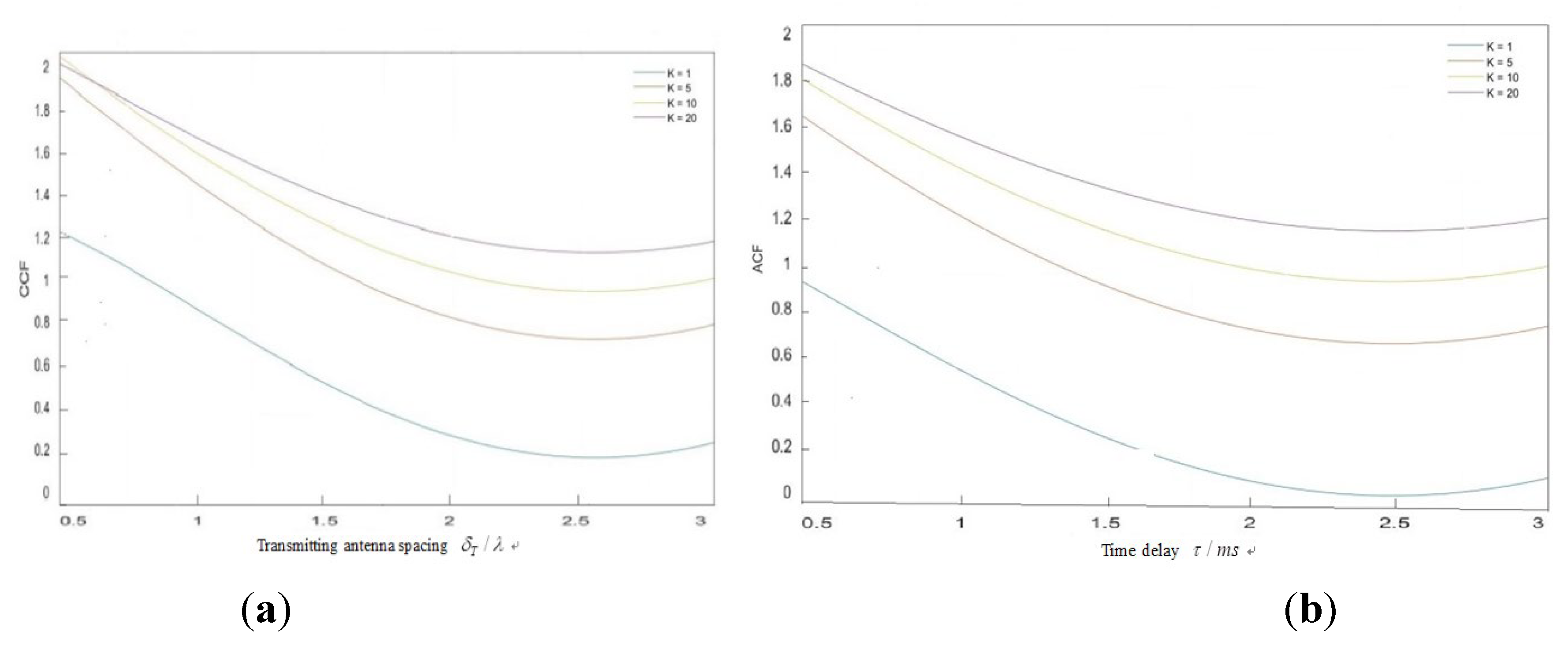

Table 1.
Definition of Channel Model Related Parameters.
| Parameter | Significance |
|---|---|
| The distance between the transmitting end and the receiving end | |
| , | The spatial position of the transmitting antenna and receiving antenna |
| ,, | Tube radius, length of sphere radius around and |
| , | The azimuth angle of and antennas |
| , | Elevation angles of and antennas |
| The moving speed of antenna | |
|
,(i=1,2,3) |
The departure azimuth from the transmitting end to the th scatterer and the arrival azimuth from the th scatterer to the receiving end |
| ,((i=1,2,3) | The departure angle from the transmitting end to the th scatterer and the arrival angle from the th scatterer to the receiving end |
| , | Representing the direct path arrival azimuth and arrival elevation angle respectively |
|
,, ,, |
Representing the path lengths between separately、、、 、、separately |
| The height difference between the transmitting and receiving antennas |
Table 2.
Channel model parameters.
| Parameter | Assignment |
|---|---|
| , | |
| , | |
| , | |
Disclaimer/Publisher’s Note: The statements, opinions and data contained in all publications are solely those of the individual author(s) and contributor(s) and not of MDPI and/or the editor(s). MDPI and/or the editor(s) disclaim responsibility for any injury to people or property resulting from any ideas, methods, instructions or products referred to in the content. |
© 2025 by the authors. Licensee MDPI, Basel, Switzerland. This article is an open access article distributed under the terms and conditions of the Creative Commons Attribution (CC BY) license (http://creativecommons.org/licenses/by/4.0/).
Copyright: This open access article is published under a Creative Commons CC BY 4.0 license, which permit the free download, distribution, and reuse, provided that the author and preprint are cited in any reuse.


