
Submitted:
17 February 2025
Posted:
18 February 2025
You are already at the latest version
Abstract
Two reservoir's porosity datasets are mapped using the Polynomial Regression (zonal estimation), Inverse Distance Weighting and Ordinary Kriging (both are interpolations). Data are taken in the sandstone reservoirs named as "K" (19 data) and "L" (25 data), of the Lower Pontian age, and located in the Sava Depression, Croatia. Maps are compared using cross-validation, based on the mean square error, and visually inspecting the main map features. Datasets are considered as small ("K" reservoir) and large ("L" reservoir). In the "K" reservoir, the MSE values are 0.00119 for IDW vs. 0.5401 for PR. In the "L" res-ervoir the MSE are 0.000676 (OK) vs. 0.0401688 (PR). Zonal estimation obviously did not prove as primary mapping in the sets with about 20 data. The linear interpolator like the IDW or OK are much better choices, especially if spatial model can be reliably modelled, like in this case for porosity characterised with normal distribution, what favoured the OK. However, zonal interpolation can be useful addon in interpretation, especially in zones where interpolation is considering less reliable and transitional areas cannot be used as base for further development.
Keywords:
sandstone reservoirs
; porosity
; zonal estimation
; interpolation
; Sava Depression
; Croatia
1. Introduction
The fluid's reservoir modelling is closely based on understanding spatial variations of numerous geological variables like porosity, permeability, saturation, mineral and lithological content. Better knowledge leads to better and longer recovering. Such data are, often, very scarce and irregularly distributed what makes it difficult to interpret them. Also, the most of them are indirectly calculated what complicates their reliability. It puts dilemma in selection of the interpolation methods, which are practically one of the most important interpretative tools.
Here are analysed two datasets, one with 19 (reservoir "L"), and another with 25 (reservoir "K") data, what make them small and larger [1] datasets, retrospectively. Both include porosity values calculated (from logs and cores) as reservoir's averages in real wells and represents the most important available variable for spatial mapping. Regular geological mapping can be done with any number of data, however dozens of them make maps reliable. In subsurface fluid reservoir's mapping such plentiful of data is rarely available, and 10 or so are datasets that need to be handled, more or less, successful for development and recovery prediction. In such cases methods like Kriging are less useful than mathematically simpler like Inverse Distance Weighting (IDW). Also, interpolation often, in very uncertain datasets (because of statistics or data sources), can be replaced with even more basic approach on the zonal estimation. Here are used both of such approach as test for "average" reservoir in the selected area, looking for answer about the most appropriate approach when can be chosen zonal estimation (Polynomial Regression; PR), simpler interpolation (IDW) or more advanced interpolation (Ordinary Kriging; OK).
Analysed reservoirs are chosen in the Croatian part of the Pannonian Basin System (CPBS), i.e., in the western part of the Sava Depression (Figure 1), where numerous hydrocarbon fields had been discovered, and many of them are still in production. Both ae of the Lower Pontian age and mostly consist of the medium-grained sandstones.
And last, but not the least, mentioned methods are widely used in geological researching, even in the CPBS. However, they are not limited only to geology, just the opposite. For example, application of the PR can be found in the medicine [3,4], biology [5], chemistry [6], psychology [7], geography [8], meteorology [9], thermodynamics [10], mechanical engineering [11,12], astronomy and astrophysics [13], computing [14,15], economics [16,17], civil engineering [18], food technology [19], agriculture [20], ecology [21,22], petroleum industry [23,24,25,26,27,28] and other.
Furthermore, the Inverse Distance Weighting method has found applications in geography [29], meteorology [30], geology [31], electrical engineering [32], and computing [33]. The success of Ordinary Kriging is also not limited to a specific field, as it has been applied in medicine [34], geography [35], geostatistics [36], environmental science [37], and economics [38].
2. Geological Settings and Location
The PBS, macro unit of the largest order, encompasses areas in eight countries, generally in the Central Europe. That system is surrounded by Carpathian, Alps and Dinarides as the regional mountain chains (orogens). The PBS starting to be created during the Ottnangian due to convergence between Euroasian and African Plates, i.e., subduction of the Apulian Plate below the Dinarides. So, the PBS is typical back-arc basin system, covered with numerous marine and lacustric environments, among which the largest was the (part of) Paratethys [39].
The CPBS (Figure 2), at the south-west margin, includes four geological macro units of the 2nd order, namely Mura, Drava, Sava and Slavonia-Srijem Depressions. There are discovered about 40 hydrocarbon fields with numerous reservoirs, mostly in the Neogene (Upper Miocene) sandstones.
In the CPBS, two main lithological macro sequences dominate. Their differentiation has been established based on lithology and geological history [40]. The 1st, younger, includes mostly clastic sediments, with minor biochemical (like Lithotamnium limestones) or magmatic (like basalts), of the Neogene and Quaternary periods. The 2nd, older, in the bottom is significantly older, from Mesozoic or Palaeozoic eras, encompassing magmatic or sediment rocks, often metamorphosised. The 1st sequence, in the Sava Depression, is divided into six lithostratigraphic formation [41], where 3 of them, important for this researching, are presented on the Figure 3.
During the entire Neogene—Quaternary period [43] described for the CPBS two transtensional (Badenian and Pannonian—Early Pontian) and two transpressional (Sarmatian and Late Pontian—Quaternary) regional tectonic phases. Neogene and Quaternary cyclic sediments were divided in megacycles with lithostratigraphic formations and members. Late Miocene (Pannonian and Pontian) cycle includes sedimentary association of the Sava Group (the Ivanić-Grad, Kloštar-Ivanić and Široko Polje Formations) in the Sava and western Drava Depressions. Deposition lasted approx. 5.9 Ma, and it is represented by the sequences of grey coloured sandstones, siltites and marls. The maximum total thicknesses are deposited in the central part of depressions, pinching out toward the margins. These sandstones. siltites and marls are deposited in deep lake environment basin sedimentation interrupted with turbidites, with the main sources of the material from the Eastern Alps. Main depositional mechanisms during Late Pannonian and Early Pontian were deep water turbidites and sequences of hemipelagic marls were described as well, both in the marginal and the central parts of basins. Several facies associations has been described: turbidite channel fill facies association - thick-bedded sandstones and thin-bedded sandstones; turbidite overbank-levee facies association - laminated sandstones, siltstones and marls passing into sandstones; distal turbidite facies association - alternating thin sandstones with siltstones and marls; massive marls facies association - marls with rare intercalations of thin siltstone or sandstone laminae.
The Sava Depression has been filled with sediments since the Early Neogene. However, the analysed reservoir rocks ("K" and "L" in Figure 3) are of the Late Neogene (Lower Pontian) age and they are a part of the Kloštar-Ivanić Formation. Arenitic sandstones prevail at the base of the formation, and more fine-grained sandstones intercalated with marl appear more frequently toward the top, as well as in the overlying the Široko Polje Formation. Sandstones units (thick 20-150 m) are the main reservoir rocks, and intercalated grey to brown marls (thick from 30-150 m) present the main isolator rocks. These Lower Pontian ("Abichi beds") extend across the Sava Depression, comprising of sandstones and marls. Sandstones were deposited from turbidite currents in the largest thicknesses in the central part of the depression, while marls were deposited as turbidites were calm down and settled from suspension. Generally, there are developed several unique lithofacies resulted from Bouma sequence, namely (1) interlaminated marlstone and sandy siltite/shale, (2) laminated marlstone interchanged with clayey-calcitic laminas and laminas with mica flakes and fine quartz grains, (3) fine-grained silty lithic greywacke sandstones to mudstones with quartz grains lithic fragments, bounded in matrix. (4) silty marlstones with kerogen; (5) lithic arenite sandstones with quartz grains and lithic fragments; (6) fine-grained fossiliferous lithic arenite sandstones; (7) coarse-grained lithic arenite sandstone to petromictic breccia/conglomerate; (8) clast-supported petromictic conglomerate with sandy matrix. Locally can be recognised some of them, depending on age and palaeoenvironment, and analysed reservoirs belongs to lithofacies 5 and 6.
The analysed reservoirs "L" and "K" are located (Figure 4) at the margin of the western Sava Depression. They largely participate in the hydrocarbon potential of analysed zone. That part includes about 20 hydrocarbon fields still in production, but several others are depleted. The largest ones are the Stružec Field (16x106 m3 Original Oil In Place, abbr. OOIP) and the Ivanić Field (7x10⁶ m3 OOIP) [43]. The entire western part covers area of about 8000 km2, where surface projection of the field's areas takes about 930 km2 [44]. Generally little deeper and more to the west are located sediments described as the source rocks, with fine-grained sediments mainly enriched in kerogen. They correspond to previously described lithofacies 1, 2 and sporadically 3. All are deposited in the in deeper lacustrine environment from basin sedimentation or at the distal parts of turbidites.
3. Mathematical Basics of Applied Interpolation Methods
Here are described analytical methods applied in this researching. The Polynomial Regression is used as zonal estimator, and the Inverse Distance Weighting and Ordinary Kriging as linear interpolator. The Mean Square Error is calculated as estimator of mapping numerical error.
The polynomial regression, as estimation (here also zonal) method, had been in the focus of this paper as tools that could be useful companion in application of other linear interpolators like the IDW or OK. It could be useful when interpolation methods do not provide reliable solutions to the problem of constructing representative spatial distributions, for example in cases like low number of data, clustering or numerous outliers. Moreover, polygonal methods are considered in geostatistics (beside cell-declustering, (e.g., [46], [47]) as one of the declustering methods, where polygon of influence (known as Thiessen or Voronoi polygon, e.g., [48], [49]) includes all data points that are closer to the sample compared to any other measurements. As result, spatially separated data points will have larger polygons than clustered (grouped) ones. Such polygonal declustering, characteristics for all zonal methods have been tested on two datasets presented in this researching.
3.1. The Polynomial Regression
The polynomial regression is kind of improvement of simple linear regression, in case that the relationship between the data is non-linear. In such vase the polynomial regression can better fit data, adding some polynomial terms into linear regression equation and modelling relationship between the dependent (Y) and independent (X) variables with nth degree polynomial function. The model is called a quadratic is such polynomial is 2, a cubic for 3 (e.g., Equation 1). The degree of function order can be set on any value (sometimes this order is considered as hyperparameter as well), but selection must be done carefully because each polynomial function can be easily underfitted or overfitted (even if least square method is used for minimizing the error). There is some kind of the "rule of the thumb" that in the subsurface mapping the fitting function could not to be of the 5th or higher order. So, right polynomial degree would need to lead to reasonable mapping structures (where the main ones are confirmed with other mapping method), but also with smaller cross-validation results (when several models are run).
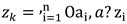
The Polynomial Regression (PR) method describes relation between independent variable x and dependent y, using polynomial of the nth order suitable for approximation of their relation [28]. The PR can be calculated using Equitation 1, e.g. [26], and is used for non-linear relations, what can help in looking for connection for more complex datasets.
 where is:
y - dependent variable;
x - independent variable;
n - the nth order of regression;
εi - error for ith data;
β - values adjusted during the calculation.
The Equation (1) represents general polynomial regression term, which always includes model parameters and hyperparameter at the end. Here is marked the "error" as the correction parameter using for fitting the model during iterations. Such parameter is used to reach optimum the model parameters. In fact, any parameter that models the function shape is called hyperparameter. It could be the ratio between training and validation datasets etc. Here such parameter is called "error", however, in the applied algorithms, the more important hyperparameter is the order of the fitting function, named as the Maximum Total Order (MTO). Here it is tested with several values between 1 to 10, optimising the regression model through iterative model. The goal was to find the best value of hyperparameter, leading to the optimal map.
3.2. The Inverse Distance Weighting
The Inverse Distance Weighting (IDW) is relatively simple linear interpolation where unknown value is calculated from known data inside searching radius, and assumption that closer data stronger participate in interpolation of unknown value. The interpolation of the unknown is defined by Equation (2), e.g., [50]:
 where is:
ZIU - interpolated value;
di - distance to ith location;
zi - known value at the ith location;
p - distance exponent.
It is obvious that interpolation is highly depended on distance exponent (p) and its selection is led by obtaining the logical visual shapes on the map as well as minimal numerical error. In mapping it is very often set on value 2 [51], especially subsurface geological mapping in the Northern Croatia [e.g., 1,42,52,53].
3.3. The Ordinary Kriging
General linear equitation is given in (3), e.g., [54], where higher value of the weighting coefficient points on known value closer to location where value is estimated.
 where is:
zk - value estimated at location „k“;
λi - weighting coefficient at location „i“;
zi - measured value at location „i“.
The Ordinary Kriging (OK) equation is upgraded Simple Kriging (SK) with adding of the Lagrange factor (µ), aiming to minimizing the Kriging variance. Surely, both techniques minimizing variance, but the OK is more successful if is rightly applied. Also, all other Kriging techniques (like Universal, Disjunctive, Indicator...) has some adding "factors" with the same purpose, designed for the specific analyses. The SK is only algorithm where sum of weightings is not standardised at 1. Also, in the SK the mean is known, but global, and in the OK the local one is used. Eventually, in all Kriging techniques (except of Indicator) the normal distribution of input dataset is highly recommended for more reliable results. It is closely connected with requirements of the stationarity of the 2nd order where is implied that expectation is independent on number and locations of data, and covariance is dependent only on distances among data (variogram). Only the Indicator Kriging assumed the stationarity of the 3rd order that implied independency of expectation and variogram existence (intrinsic hypothesis). The Lagrange function is represented with Equation 4:
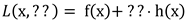 where is: L(x,µ) -Lagrange function;
f(x), h(x) - functions for the "x" values;
µ - Lagrange factor.
Now, the Ordinary Kriging matrix equation can be presented with Equation 5 [e.g., 55]:
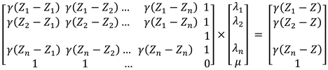 where is:
γ - variogram values;
Z1....Zn – measured values at locations "1...n";
Z – locations where new value is estimated;
μ – Lagrange factor.
The mentioned property of the Ordinary Kriging is that technique works with local mean (not global), what can be pretty good feature for mapping geological subsurface data, at least in the CPBS [56]. It is pure deterministic methods as well as Inverse Distance and Polynomial Regression, for example. All are "numerical and subjective", and sure, the stationarity (on some order) can be criteria for choosing the right Kriging technique if researcher knows how to observe stationarity.
3.4. The Cross-Validation
The cross-validation (CV) is set of techniques applied for estimation error calculation. Here is selected the mean square error (MSE) technique as one of the most applied in comparison of several interpolations for the same dataset. As measure of residuals variance, it usually means that the lower MSE would lead to conclusion about better interpolation. There are also some other measures, like mean absolute error (MAE, the average of the absolute difference between measured and estimated values, i.e., residuals average), root mean square error (RMSE, keeping the same unit as input dataset, allowing easier interpretation) etc.
The MSE is iterative procedure where one, randomly selected, measured values is ignored and at the same location its value is again estimated (with selected interpolation method) from the rest of measurements. The difference between those two values is error in that point. The procedure is repealed for all other measured values and eventually the MSE is calculated using Equation 6, e.g., [57]:
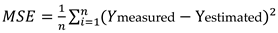 where is:
MSE - mean square error (of the estimation);
N - number of data;
Ymjereni,i - measured value for loaction "i";
Yprocijenjeni,i - estimated value for location "i".
However, the interpretation is not so straightforward, because the maps also can include different isolines shapes, where some forms (structures) could be almost impossible and could eliminate interpolation method although the accompanied MSE is lower than in other methods.
4. Discussion and Results Overview
This researching has been focused on zonal estimation as useful addon to classical interpolation methods in the hydrocarbon sandstone reservoirs. The goal has been set up for the CPBS, where numerous interpolations of mentioned and similar reservoirs had been published. The PR is selected as zonal estimation. The IDW and OK are used interpolations. The datasets are divided into small (19 data, Table 1) and large (25 data, Table 2) although both are of similar size.
Both sets are limited in their representation, but also solely publicly available for analysed zones. Given values are mostly derived indirectly from e-logs, and it is why they are same in the numerous wells. In reality, they are very similar because logged in the same lithofacies. Values represent mean porosity along entire reservoir in the corresponding well, what is often used in numerous mappings. However, some practitioners used porosities pondered with another variables, for example, thickness. Such option is not correct to apply if the researcher does not know (and described) depositional model, i.e., how clastics volume and sizes depends on (well) position in such environment and subsequent compaction. As we did not have such detail information, the pure mean porosity has been mapped.
Listed data had been interpolated or estimated using IDW, OK and PR. Table 3 presents the cross-validation values obtained by changing the value of the maximum total order (MTO). The selected MTO (as previously mentioned as one hyperparameter related on the order of a fitting function) values are 1, 2, 3, 4, 5, and 10. They determine the maximum sum of the exponents of the independent (X) and (dependent) Y variables, i.e., the degree of polynomial regression, ensuring that the sum of the exponents does not exceed the MTO value [58]. For example, for "n" data, the maximum degree of polynomial function and MTO is "n-1". Like it was mentioned for order of the polynomial function, choosing an excessively high MTO value may lead to over-fitting which causes situations where the data or predictions have significant errors or variations, which makes them unreliable [59]. In contrast, a low value of MTO may result in under-fitting of the model leading to failure in representing the relationship between the variables [60]. For all cases the MSE is calculated and maps generated. Regarding the PR there were several options to estimate data changing the option named as "Max Total Order (MTO)". In this analysis such option is varied with values 1, 2, 3, 4, 5 and 10, looking the lowest MSE (Table 3).
When MTO reached 2, the MSE staying constant (and overall, the variations are too small that it is matter). So, this parameter can be considered of low importance, when sill of 2 is reached, for used datasets regarding their abundance and locations. The next step was calculation of the same error using the IDW and OK interpolations in the same reservoirs (Table 4).
In both reservoirs the MSE values are considerably lower for interpolations than for estimator (Table 3 and Table 4). In the reservoir "K" the MSE values are 0.000119 (IDW) and 0.05401 (PR). In the reservoir "L" the MSE are 0.000676 (OK) and 0.040117 (PR). In the reservoir with more data those values are absolutely lower, what indicated on statistically representative datasets, i.e., fact that increasing of values did not include new "outlier" values and confirmed that both datasets are representative. Also, the lowest MSE for OK proved that 25 data were enough abundant for calculation of reliable spatial model (variogram) based (probably, because it is not tested) normal distribution of porosity (as theoretical assumption for sandstone reservoirs).
The maps made for both datasets using the PR zonal estimator are shown on Figure 5a (reservoir "K") and Figure 5b (reservoir "L"). The main difference is, like as in the MSE, in map associate with MTO=1 and maps with MTO>1. As zonal, the maps show sharp borders between different porosity zones and all follow the NW-SE/WNW-ESE strike, what corresponds with the strike of sandstone depositional environment. For reservoir "K" (Figure 5a) the zone values (colours) are almost the same for the MTO=2, 3 and 10, what follows the stabilisation of the MSE on the MTO=2 and higher. For the reservoir "L" almost the same statement is valid, also with additional features reflected in the "parabolic" borders among zones. Also, the PR is sensitive on higher differences between close data, what is visible in well pairs J-168 and J-25, i.e., L-27 and L-131a. In any case when the data are classified mostly in several groups of the same values (Table 1 and Table 2) the zonal estimator will group them pretty clear and simple.
The interpolated maps are given on Figure 6a (reservoir "K", the IDW) and Figure 6b (reservoir "L", the OK). As expected, the interpolators are based on transitional zones between isoporosity lines on the selected equidistance. So, the spatial interpretation and prediction is much easier than in the zonal representation, however, can be tricky when numerous points are of the same values like in the presented reservoirs (Table 1 and Table 2). The main difference is existing of the maximums and minimums, which on the zonal maps were amalgamated into single zone. Back to MSE it would be more appropriate spatial solution than zones.
Application of the OK asked for definition of spatial model, what was not easy task due to relatively low amount of data. It is why the omnidirectional variogam model had been used (for directional there would not be enough data per sectors of the searching ellipsoid). Some theoretical variogram models (Figure 7) had been tested like linear (range about 900 m) and spherical (range about 350 m) with relatively small changes in visual results and MSE. So, we prefer to use models with lower ranges. Also, the Kriged map used larger equidistance (0.02) than the IDW (0.01) just to be sure that different spatial model will not significantly change the shapes of the main "structures". It was not influenced the MSE calculation.
5. Conclusions
The main achievements can be summarised as follows:
1. Zonal estimators and interpolators are two different approaches for subsurface sandstone mapping, both with their own properties and advantages.
2. Larger datasets will favour interpolators, smaller estimators.
3. Here is proven that both datasets can be interpolated with the IDW (19 data, "K", 0.000119) and even using the OK (25 data, "L", 0.000676), and in both cases the MSE will be significantly lower than in the estimation with the PR (0.05401 in "K" and 0.040117 in "L").
4. However, both datasets are very specific meaning that many values are the same, what practically decreased number of different data from 19 or 25 to only several classes.
5. That is result of way how data are calculated, where they are indirectly averaged from mixture of well logs and cores in the sandstone reservoir intervals across the field.
6. In such case pure interpolation will not be so useful, because most transitional isoporosity lines are not confirmed with measured value, i.e., hard data, but are artificially calculated from interpolation algorithm between hard points (e.g., Figure 6aas area among J-25, J-168, J- 173 wells).
7. Alternatively, it could be improved with simultaneously running zonal estimator algorithm, where mentioned value's classes could be easily recognised inside zones, revealing their area and strike (Figure 5a, b).
8. Zonal maps can greatly improve development of presented sandstone reservoirs or their counterparts in other regions of the CPBS if depositional model for mapped structure is described in details.
Author Contributions
each author had made substantial contributions to the conception, analysis, or interpretation of data. All has approved the submitted version and agreed to be personally accountable for the author’s contributions. Conceptualization, J.I. and T.M.; Methodology, J.I and T.M.; Software, J.I.; Validation, T.M.; Formal Analysis, J.I., I.B., M.R. and U.B.; Writing – Original Draft Preparation, J.I., T.M., I.B., M.R., U.B.; Writing – Review & Editing, J.I., T.M., I.B., M.R., U.B.; Visualization, I.B., M.R.; Supervision, J.I.; Project Administration, T.M.
Funding
This research received no external funding.
Institutional Review Board Statement
Not applicable.
Informed Consent Statement
Not applicable.
Data Availability Statement
The original theses, from which data and methodologies are derived, will be included in the Faculty of Mining, Geology and Petroleum Engineering Repository, University of Zagreb, Croatia. Repository gathers, permanently stores and allows open access to digital versions of researching theses of its employees and students. Further inquirers can be directed to the corresponding author.
Acknowledgments
This research was partly carried out within the framework of the projects “Mathematical Research in Geology IX/2024” (led by T. Malvić) and for bachelor theses of Ivana Brajnović and Maria Rudec (co-mentoring by J. Ivšinović & T. Malvić)..
Conflicts of Interest
The authors declare no conflicts of interest.
Abbreviations
The following abbreviations are used in this manuscript:
| OK | Ordinary Kriging |
| SK | Simple Kriging |
| IDW | Inverse Distance Weighting |
| PR | Polynomial Regression |
| MSE | Mean Square Error |
| PBS | Pannonian Basin System |
| CPBS | Croatian part of the Pannonian Basin System |
References
- Malvić, T.; Ivšinović, J.; Velić, J.; Rajić, R. Interpolation of Small Datasets in the Sandstone Hydrocarbon Reservoirs, Case Study of the Sava Depression, Croatia. Geosciences 2019, 9, 201. [Google Scholar] [CrossRef]
- Malvić, T.; Pimenta Dinis, M.A.; Velić, J.; Sremac, J.; Ivšinović, J.; Bošnjak, M.; Barudžija, U.; Veinović, Ž.; Sousa, H.F.P.e. Geological Risk Calculation through Probability of Success (PoS), Applied to Radioactive Waste Disposal in Deep Wells: A Conceptual Study in the Pre-Neogene Basement in the Northern Croatia. Processes 2020, 8, 755. [Google Scholar] [CrossRef]
- Hung, C.-Y.; Newton Fernando, O.N.; Wang, C.-Y.; Chen, K.-W.; Samani, H.; Yang, C.-Y. Improving Clinical Decision-Making with Polynomial Regression-Based Real Patient State Estimation. International Automatic Control Conference (CACS), Penghu, Taiwan, 2023.
- Srilakshmi, U.; Manikandan, J.; Velagapudi, T.; Abhinav, G.; Kumar, T.; Saideep, D. A New Approach to Computationally-Successful Linear and Polynomial Regression Analytics of Large Data in Medicine. Journal of Computer Allied Intelligence 2024, 2, 35–48. [Google Scholar] [CrossRef]
- Ma, L.; Zheng, J. A polynomial based model for cell fate prediction in human diseases. BMC Syst Biol 2017, 11 (Suppl. S7), 126. [Google Scholar] [CrossRef]
- Frisbie, S.H.; Mitchell, E.; Sikora, K.R.; Abualrub, M.; Abosalem, Y.M. Using Polynomial Regression to Objectively Test the Fit of Calibration Curves in Analytical Chemistry. International Journal of Applied Mathematics and Theoretical Physics 2016, 1, 14–18. [Google Scholar] [CrossRef]
- Visser, L.; Pat-El, R.; Lataster, J.; Van Lankveld, J.; Jacobs, N. Beyond Difference Scores: Unlocking Insights with Polynomial Regression in Studies on the Effects of Implicit-Explicit Congruency. Psychologica Belgica 2024, 64, 5–23. [Google Scholar] [CrossRef]
- Najafzadeh, M.; Kargar, A.R. Gene-Expression Programming, Evolutionary Polynomial Regression, and Model Tree to Evaluate Local Scour Depth at Culvert Outlets. Journal of Pipeline Systems Engineering and Practice 2019, 10. [Google Scholar] [CrossRef]
- Weslati, O.; Bouaziz, S.; Serbaji, M.M. The Efficiency of Polynomial Regression Algorithms and Pearson Correlation (r) in Visualizing and Forecasting Weather Change Scenarios. In Recent Advances in Polynomials. 2022. pp. 20.
- Bal, S.; R. R. Prediction Of Heat Transfer Performance Using Polynomial Regression. Second International Conference on Artificial Intelligence and Smart Energy (ICAIS), Coimbatore, India, 2022, pp. 1735–1740.
- Trebuňa, F.; Ostertagová, E.; Frankovský, P.; Ostertag, O. Application of Polynomial Regression Models in Prediction of Residual Stresses of a Transversal Beam. American Journal of Mechanical Engineering 2016, 4, 247–251. [Google Scholar]
- Wu, S.; Zhang, T. Active Learning Model on Wind Turbine Power Generation Based on Polynomial Regression. In Proceedings of the 2021 5th International Conference on Deep Learning Technologies (ICDLT '21). Association for Computing Machinery, New York, NY, USA, 2021, 111–115.
- Jiménez-López, D.; Corcho-Caballero, P.; Zamora, S.; Ascasibar, Y. Polynomial expansion of the star formation history in galaxies. Astronomy & Astrophysics 2021. [Google Scholar] [CrossRef]
- Huang, L.; Jia, J.; Yu, B.; Chun, B.-G.; Maniatis, P.; Naik, M. Predicting execution time of computer programs using sparse polynomial regression. In Proceedings of the 24th Annual Conference on Neural Information Processing Systems, 2010.
- Mustafa, S.; Aziz, M.; Ahmed, D.R. Software Reliability Assessment Using Polynomial Regression Approach. In Proceedings of ICATCES, 2020.
- Mo, H. Comparative Analysis of Linear Regression, Polynomial Regression, and ARIMA Model for Short-term Stock Price Forecasting. Advances in Economics Management and Political Sciences 2023, 49, 166–175. [Google Scholar] [CrossRef]
- Adeboye, N.O.; Agunbiade, D.A.; Adeniran, B.G. A Polynomial Regression Model of Monetary Policy Rate in Nigerian Economy. British Journal of Science 2014, 11, 11. [Google Scholar]
- Golnaraghi, S.; Moselhi, O.; Alkass, S.; Zangenehmadar, Z. Modelling construction labour productivity using evolutionary polynomial regression. International Journal of Productivity and Quality Management 2020, 31, 207–226. [Google Scholar] [CrossRef]
- Yanova, M.A.; Oleynikova, E.N.; Khizhnyak, S.V. Polynomial regression as a tool for prediction quality of bread baked of wheat flour mixed with flour of cereal extrudates. IOP Conf. Ser. : Earth Environ. Sci. 2019, 315. [Google Scholar] [CrossRef]
- Shah, B.; Chettri, S.T.; Diyali, R.S.; H K, S.; Maharjan, S. Rain Prediction Using Polynomial Regression for the Field of Agriculture Prediction for Karnatakka. SSRN Electronic Journal 2020. [Google Scholar] [CrossRef]
- Bera, D.; Chatterjee, N.D.; Bera, S. Comparative performance of linear regression, polynomial regression and generalized additive model for canopy cover estimation in the dry deciduous forest of West Bengal. Remote Sens. Appl. Soc. Environ. 2021, 22, 100502. [Google Scholar] [CrossRef]
- Goodale, C.L.; Aber, J.D.; Ollinger, S.V. Mapping monthly precipitation, temperature, and solar radiation for Ireland with polynomial regression and a digital elevation model. Climate Research 1998, 10, 35–49. [Google Scholar] [CrossRef]
- Said, L. Forecasting Reservoir Pressure for Vertical Oil Well Using Supervised Machine Learning Model. SPE/IADC Middle East Drilling Technology Conference and Exhibition, Abu Dhabi, UAE, 2023.
- Al-Mudhafar, W.J.; Dalton, C.A.; Al Musabeh, M.I. Metamodeling via Hybridized Particle Swarm with Polynomial and Splines Regression for Optimization of CO2-EOR in Unconventional Oil Reservoirs. SPE Reservoir Characterisation and Simulation Conference and Exhibition, Abu Dhabi, UAE, 2017.
- Kalla, S.; White, C.D. Efficient Design of Reservoir Simulation Studies for Development and Optimization. SPE Res Eval & Eng 2007, 10, 629–637. [Google Scholar]
- Yao, C.; Ren, X.; Valiveti, D.; Ryu, S.; Chaney, C.; Zeng, Y. Machine Learning Based FPSO Topsides Weight Estimation for a Project on an Early Stage (OTC-32304-MS). Offshore Technology Conference, 2023.
- Aminian, K.; Ameri, S.; Abbitt, W.E.; Cunningham, L.E. Polynomial Approximations for Gas Pseudopressure and Pseudotime (SPE-23439-MS). SPE Eastern Regional Meeing, 1991.
- Wang, J.; Li, C.; Cheng, P.; Yu, J.; Cheng, C.; Ozbayoglu, E.; Baldino, S. Data Integration Enabling Advanced Machine Learning ROP Predictions and its Applications (OTC-35395-MS). Offshore Technology Conference, 2024.
- Moeletsi, M.; Shabalala, Z.; Nysschen, G.; Walker, S. Evaluation of an inverse distance weighting method for patching daily and dekadal rainfall over the Free State Province, South Africa. Water SA 2016, 42, 466–474. [Google Scholar] [CrossRef]
- Chen, F.-W.; Liu, C.-W. Estimation of the spatial rainfall distribution using inverse distance weighting (IDW) in the middle of Taiwan. Paddy and Water Environment 2012, 10, 209–222. [Google Scholar] [CrossRef]
- Bokati, L.; Velasco, A.; Kreinovich, V. Scale-Invariance and Fuzzy Techniques Explain the Empirical Success of Inverse Distance Weighting and of Dual Inverse Distance Weighting in Geosciences. North American Fuzzy Information Processing Society Annual Conference, Halifax, NS, Canada, 2022.
- Barlak, C.; Ozkazanc, Y. Battery capacity estimation with inverse distance weighting. Communications Faculty of Sciences University of Ankara Series A2-A3 Physical Sciences and Engineering, 2011, 52, 1–16. [Google Scholar]
- Çatalbaş, C.; Gulten, A. A novel super-resolution approach for computed tomography images by inverse distance weighting method. Journal of the Faculty of Engineering and Architecture of Gazi University 2018, 33, 697–711. [Google Scholar]
- Meliyana, S.; Ahmar, A. Analysis of the Distribution of Diarrhea Patients in Bogor Regency Month Using the Ordinary Kriging Method. ARRUS Journal of Social Sciences and Humanities, 2023, 3, 156–162. [Google Scholar] [CrossRef]
- Rohma, N. Estimation of Ordinary Kriging Method with Jackknife Technique on Rainfall Data in Malang Raya. International Journal on Information and Communication Technology (IJoICT), 2022, 8, 22–39. [Google Scholar] [CrossRef]
- Di, J.; Xu, J.; Fu, J.; Li, B.; Wu, M. Study on the regional ASF prediction method based on the ordinary kriging interpolation. Physica Scripta, 2023, 99. [Google Scholar] [CrossRef]
- Qiao, P.; Lei, M.; Yang, S.; et al. Comparing ordinary kriging and inverse distance weighting for soil as pollution in Beijing. Environ Sci Pollut Res 2018, 25, 15597–15608. [Google Scholar] [CrossRef]
- Awuku, B.; Asa, E.; Twum, E. Conceptual cost estimation of highway bid unit prices using ordinary kriging. International Journal of Construction Management 2022, 24, 1–10. [Google Scholar] [CrossRef]
- Malvić, T.; Velić, J. Geologija ležišta fluida (Geology of reservoir's fluids), Zagreb, 2008. Rudarsko-geološko-naftni fakultet, Sveučilište u Zagrebu.
- Velić, J.; Malvić, T.; Cvetković, M.; Vrbanac, B. Reservoir Geology, Hydrocarbon Reserves and Production in the Croatian part of the Pannonian Basin System. Geologia Croatica 2012, 65, 91–101. [Google Scholar] [CrossRef]
- Velić, J. Geology of Oil and Gas Reservoir, Zagreb, 2007. Faculty of Mining, Geology and Petroleum Engineering, University of Zagreb, Zagreb.
- Ivšinović, J.; Malvić, T. Application of the Radial Basis Function interpolation method in selected reservoirs of the Croatian part of the Pannonian Basin System. Mining of Mineral Deposits 2020, 14, 37–42. [Google Scholar] [CrossRef]
- Malvić, T.; Velić, J. Neogene Tectonics in Croatian Part of the Pannonian Basin and Reflectance in Hydrocarbon Accumulations. In: New Frontiers in Tectonic Research At the Midst of Plate Convergence (ed. Schattner, U.), InTech, Rijeka, 2011, 215-238.
- Ivšinović, J. Odabir i geomatematička obradba varijabli za skupove manje od 50 podataka pri kreiranju poboljšanoga dubinskogeološkoga modela na primjeru iz zapadnoga dijela Savske depresije (Selection and geomathematical calculation of variables for sets with less than 50 data regarding the creation of an improved subsurface model, case study from the western part of the Sava Depression), disertation. – in Croatian, Faculty of Mining, Geology and Petroleum Engineering, University of Zagreb, Zagreb, 2019.
- Ivšinović, J.; Malvić, T.; Velić, J.; Sremac, J. Geological Probability of Success (POS), case study in the Late Miocene structures of the western part of the Sava Depression, Croatia. Arab J Geosci 2020, 13, 714. [Google Scholar] [CrossRef]
- Journel, A.G. Nonparametric estimation of spatial distributions. Mathematical Geology 1983, 15, 445–468. [Google Scholar] [CrossRef]
- Deutsch, C.V. DECLUS: A FORTRAN 77 program for determining optimum spatial declustering weights. Computers & Geosciences 1989, 15, 325–332. [Google Scholar] [CrossRef]
- Chow, V.T. Handbook of applied hydrology: A compendium of water-resources technology, McGraw-Hill, 1493 pp., New York, 1964.
- Boots, B.N. Modifying Thiessen Polygons. The Canadian Geographer 1987, 31, 160–169. [Google Scholar] [CrossRef]
- Setianto, A.; Triandini, T. Comparison of kriging and inverse distance weighted (IDW) interpolation methods in lineament extraction and analysis. Journal of Applied Geology 2013, 5, 21–29. [Google Scholar] [CrossRef]
- Ly, S.; Charles, C.; Degre, A. Geostatistical interpolation of daily rainfall at catchment scale: The use of several variogram models in the Ourthe and Ambleve catchments, Belgium. Hydrology and Earth System Sciences 2011, 15, 2259–2274. [Google Scholar] [CrossRef]
- Ivšinović, J.; Malvić, T. Comparison of Mapping Efficiency for Small Datasets using Inverse Distance Weighting vs. Moving Average, Northern Croatia Miocene Hydrocarbon Reservoir. Geologija, 65, 2022, 1, 47–57. [Google Scholar] [CrossRef]
- Andrić, K.; Malvić, T.; Velić, J.; Barudžija, U.; Rajić, R. Poboljšana analiza i kartiranje geokemijskih i geoloških varijabli u prostoru Bjelovarske subdepresije (Sjeverna Hrvatska), primjenom metode inverzne udaljenosti. 2021.
- Novak, K. Modeliranje površinskoga transporta i geološki aspekti skladištenja ugljikova dioksida u neogenska pješčenjačka ležišta Sjeverne Hrvatske na primjeru polja Ivanić (Surface transportation modelling and geological aspects of carbon-dioxide storage into Northern Croatian neogene sandstone reservoirs, case study Ivanić field), disertation. – in Croatian, Faculty of Mining, Geology and Petroleum Engineering, University of Zagreb, Zagreb, 2015.
- Mesić Kiš, I. Comparison of ordinary and universal kriging interpolation techniques on a depth variable (a case of linear spatial trend), case study of the Šandrovac field. Rudarsko-geološko-naftni zbornik 2016, 31, 41–58. [Google Scholar] [CrossRef]
- Mesić Kiš, I.; Malvić, T. Variables selection and linear equations calculation for description of geological surface regional dip. Zbornik sažetaka međunarodne izložbe Inova 2016. [Google Scholar]
- Hodson, T.O. Root-mean-square error (RMSE) or mean absolute error (MAE): When to use them or not. Geoscientific Model Development 2022, 15, 5481–5487. [Google Scholar] [CrossRef]
- Draper, N.R.; Smith, H. Applied Regression Analysis, New York, 1981. A Whiley-Interscience Publication.
- Wan, X. The Influence of Polynomial Order in Logistic Regression on Decision Boundary. IOP Conference Series Earth and Environmental Science, Baubau, Indonesia 2019.
- Araújo, A. Polynomial regression with reduced over-fitting-The PALS technique. Measurement 2018, 124, 515–521. [Google Scholar] [CrossRef]
Figure 1.
Position of the Pannonian basin from [2].
Figure 1.
Position of the Pannonian basin from [2].
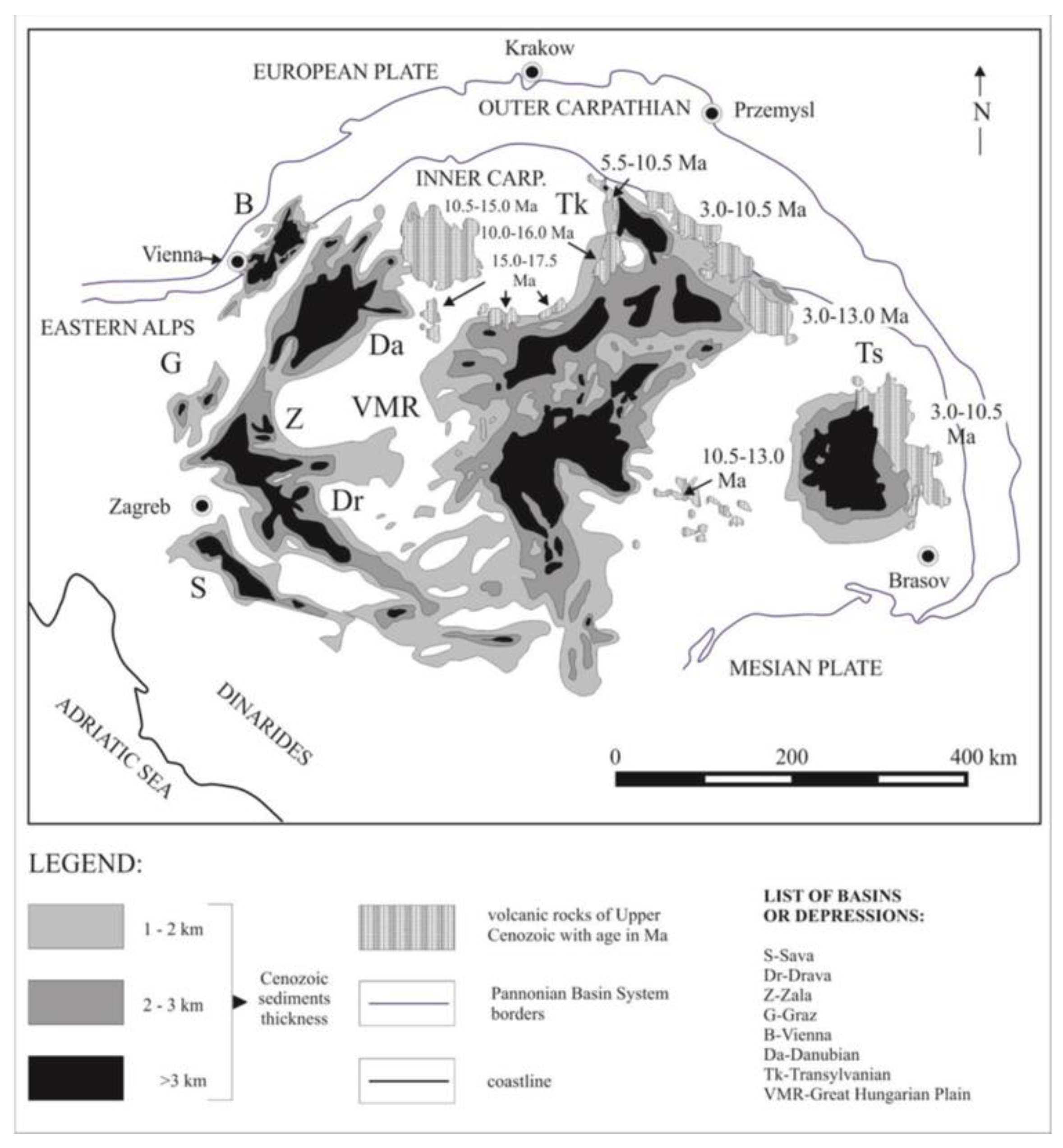
Figure 2.
Macro units in the CPBS [40].
Figure 2.
Macro units in the CPBS [40].
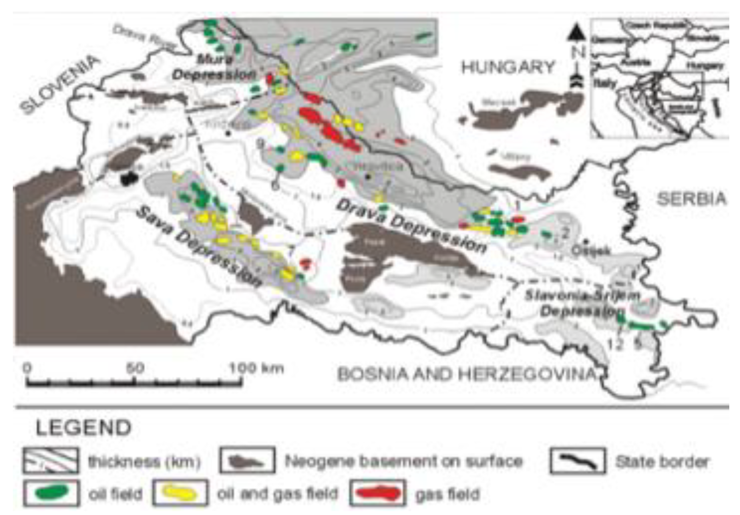
Figure 3.
Typical lithological units in the 3 younger lithostratigraphic formations of the Sava Depression [42].
Figure 3.
Typical lithological units in the 3 younger lithostratigraphic formations of the Sava Depression [42].
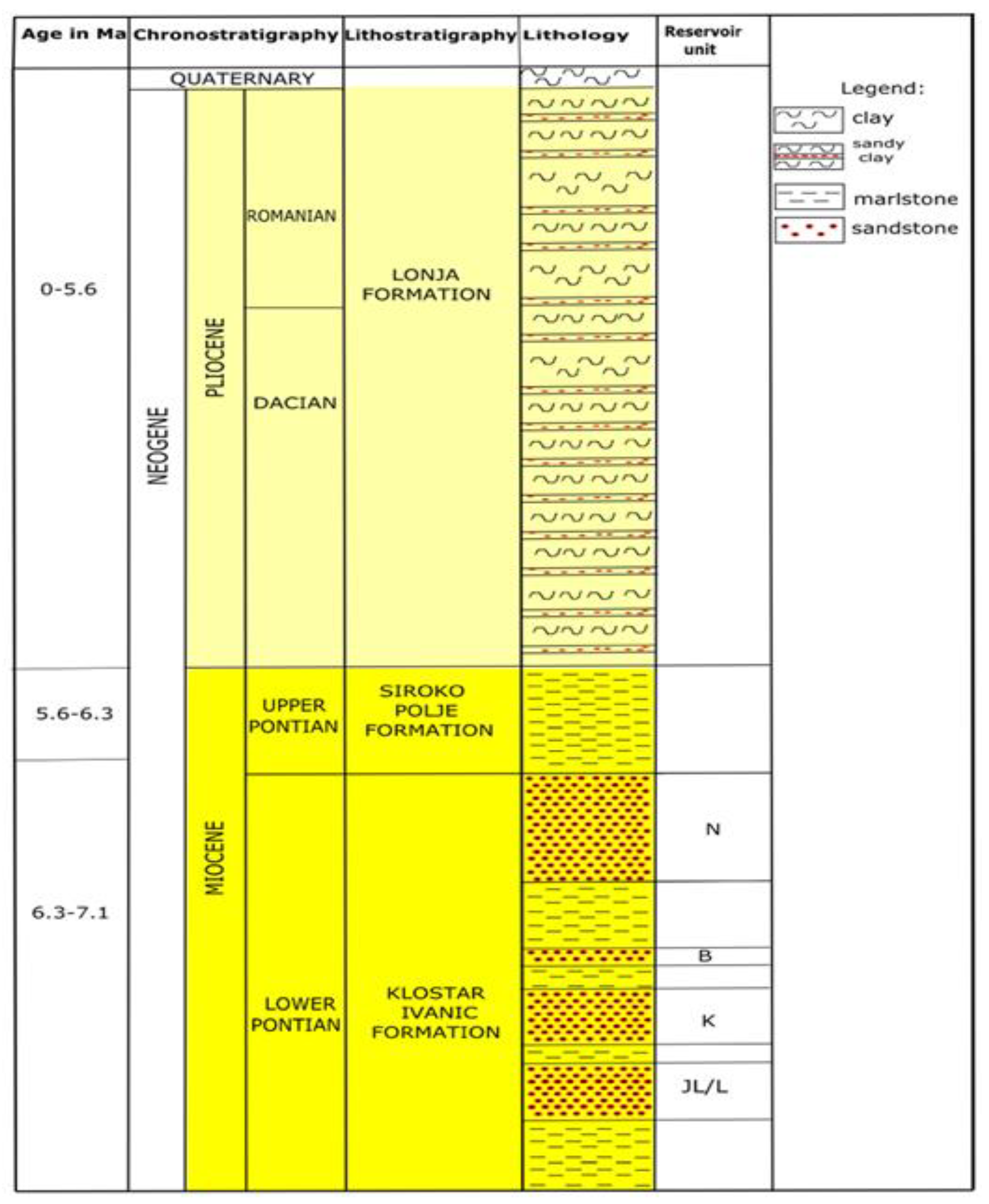
Figure 4.
Position of the western part of the Sava Depression with marked (green) analysed area from [45].
Figure 4.
Position of the western part of the Sava Depression with marked (green) analysed area from [45].
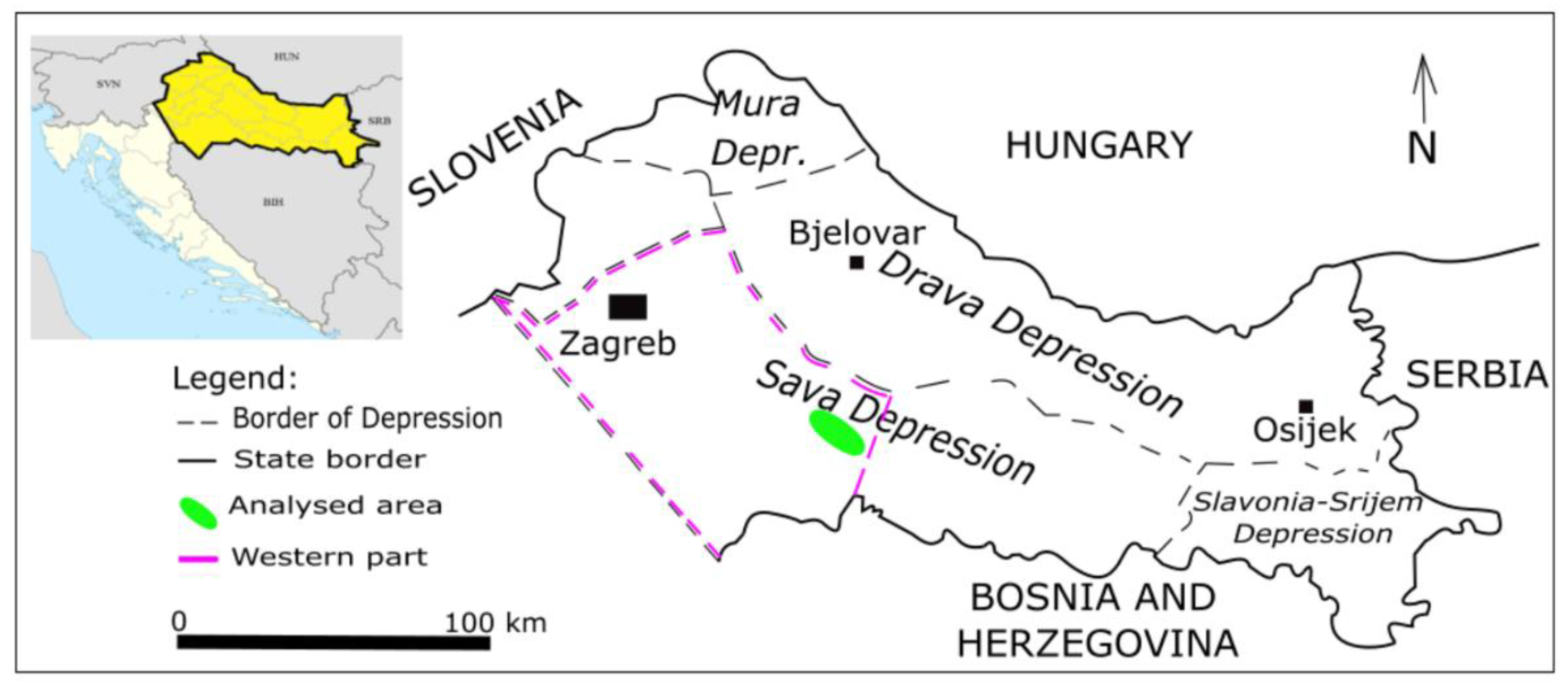
Figure 5.
The PR porosity maps with different MTO values (1, 2) for the reservoir "K" (5a - left) and the reservoir "L" (5b - right).
Figure 5.
The PR porosity maps with different MTO values (1, 2) for the reservoir "K" (5a - left) and the reservoir "L" (5b - right).
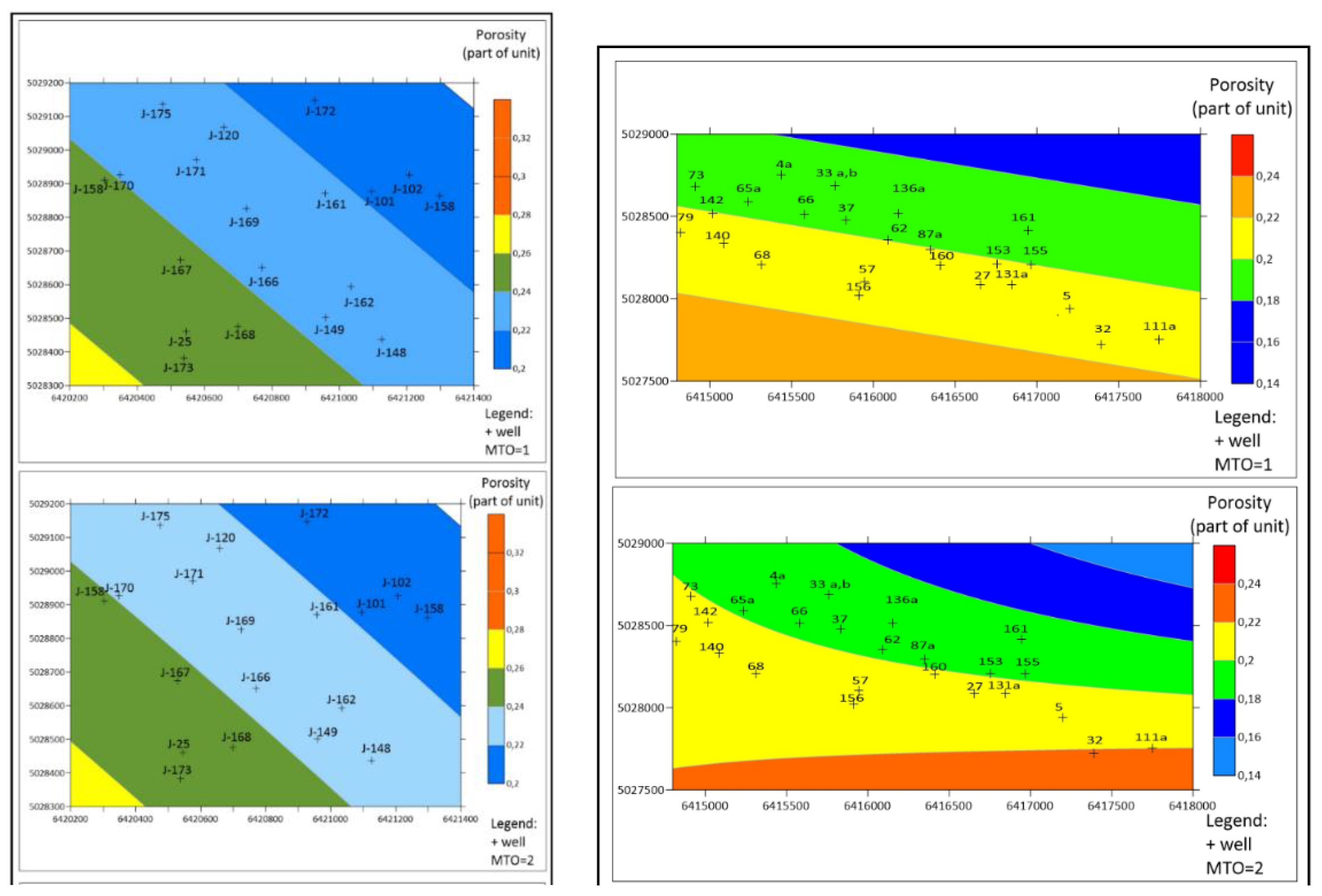
Figure 6.
The IDW porosity map for reservoir "K" (6a - top) and the OK porosity map for reservoir "L" (6b - bottom).
Figure 6.
The IDW porosity map for reservoir "K" (6a - top) and the OK porosity map for reservoir "L" (6b - bottom).
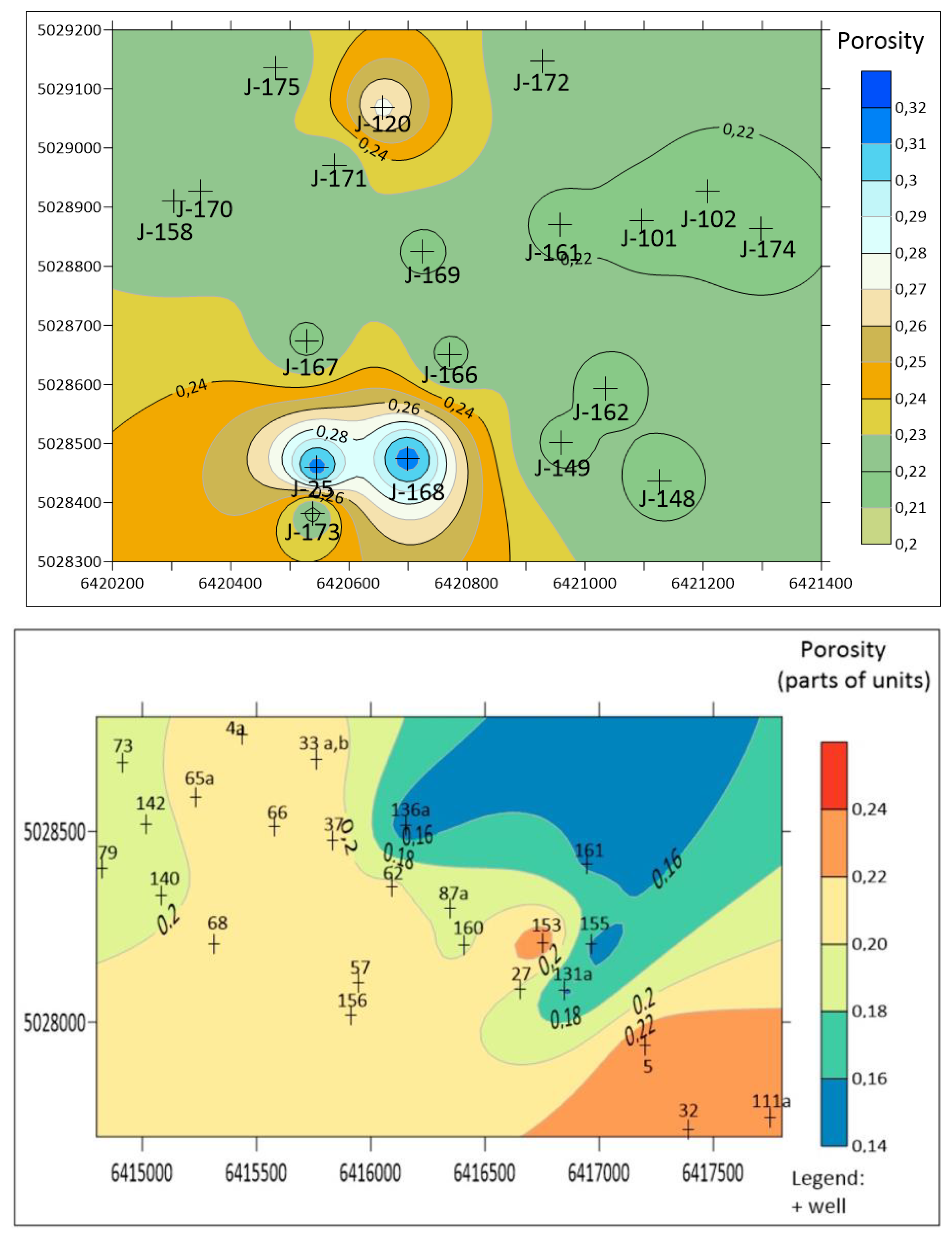
Figure 7.
Examples of some tested theoretical variogram models (linear - left, spherical - right).
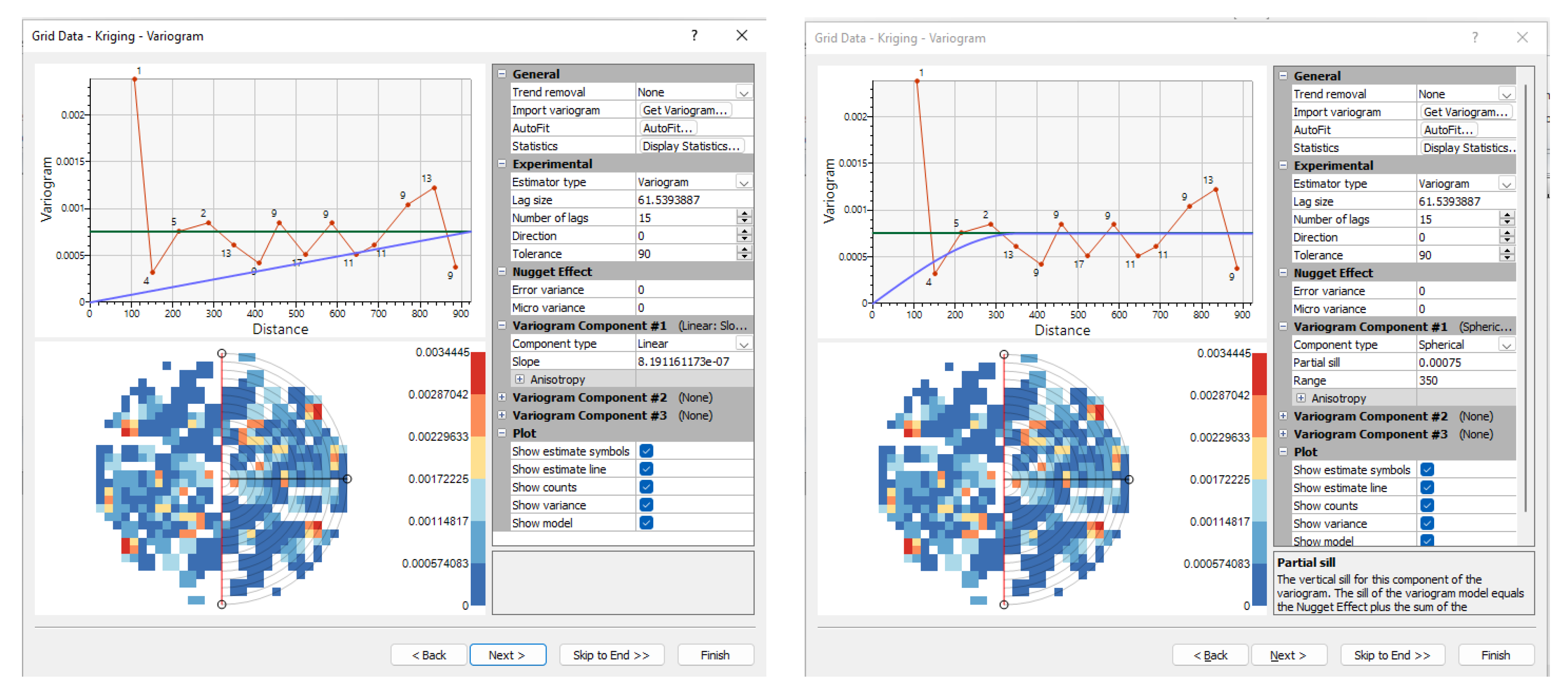

Table 1.
Porosity data for reservoir „K“.
| Name | Surface X | Surface Y | Porosity | |
|---|---|---|---|---|
| J-101 | 6421096 | 5028877 | 0.217 | |
| J-120 | 6420658 | 5029068 | 0.272 | |
| J-161 | 6420957 | 5028870 | 0.217 | |
| J-162 | 6421034 | 5028593 | 0.217 | |
| J-167 | 6420529 | 5028674 | 0.217 | |
| J-168 | 6420699 | 5028475 | 0.315 | |
| J-169 | 6420349 | 5028825 | 0.217 | |
| J-170 | 6420349 | 5028926 | 0.223 | |
| J-174 | 6421298 | 5028863 | 0.217 | |
| J-175 | 6420475 | 5029136 | 0.223 | |
| J-158 | 6420303 | 5028910 | 0.223 | |
| J-171 | 6420576 | 5028970 | 0.223 | |
| J-172 | 6420928 | 5029147 | 0.223 | |
| J-102 | 6421208 | 5028926 | 0.217 | |
| J-148 | 6421126 | 5028437 | 0.217 | |
| J-149 | 6420959 | 5028501 | 0.217 | |
| J-166 | 6420771 | 5028650 | 0.217 | |
| J-25 | 6420546 | 5028460 | 0.315 | |
| J-173 | 6420539 | 5028382 | 0.217 |
Table 2.
Porosity data for reservoir „L“.
| Name | Surface X | Surface Y | Porosity |
|---|---|---|---|
| L-111a | 6417747.87 | 5027750.49 | 0.239 |
| L-131a | 6416846.88 | 5028084.13 | 0.156 |
| L-136a | 6416153.34 | 5028514.94 | 0.145 |
| L-140 | 6415085.08 | 5028332.44 | 0.192 |
| L-142 | 6415018.82 | 5028518.52 | 0.186 |
| L-153 | 6416755 | 5028207.72 | 0.239 |
| L-155 | 6416966.63 | 5028205.04 | 0.156 |
| L-156 | 6415912.39 | 5028017.76 | 0.206 |
| L-160 | 6416409.59 | 5028202.77 | 0.197 |
| L-161 | 6416945.81 | 5028414.75 | 0.156 |
| L-27 | 6416655.05 | 5028085.51 | 0.197 |
| L-32 | 6417390.44 | 5027719.99 | 0.239 |
| L-33a | 6415763.3 | 5028687.46 | 0.214 |
| L-33b | 6415763.3 | 5028687.46 | 0.214 |
| L-37 | 6415833.62 | 5028477.16 | 0.214 |
| L-4a | 6415435.16 | 5028753.52 | 0.214 |
| L-5 | 6417199.92 | 5027939.22 | 0.239 |
| L-57 | 6415945.52 | 5028103.82 | 0.206 |
| L-62 | 6416090.56 | 5028354.65 | 0.206 |
| L-65a | 6415235.15 | 5028589.8 | 0.214 |
| L-66 | 6415579.42 | 5028511.51 | 0.214 |
| L-68 | 6415314.5 | 5028205.63 | 0.214 |
| L-73 | 6414912.05 | 5028679.32 | 0.192 |
| L-79 | 6414821.26 | 5028401.83 | 0.195 |
| L-87a | 6416346.64 | 5028297.46 | 0.917 |
Table 3.
The MSE values for the PR porosity estimation with variable MTO values, for the reservoirs „K“ and „L“.
Table 3.
The MSE values for the PR porosity estimation with variable MTO values, for the reservoirs „K“ and „L“.
| POROSITY OF RESERVOIR “K” | POROSITY OF RESERVOIR “L” | ||||
|---|---|---|---|---|---|
| DATA | MTO | MSE | Data | MTO | MSE |
| 19 | 1 | 0.054007 | 25 | 1 | 0.041100 |
| 19 | 2 | 0.054010 | 25 | 2 | 0.040168 |
| 19 | 3 | 0.054010 | 25 | 3 | 0.040168 |
| 19 | 4 | 0.054010 | 25 | 4 | 0.040168 |
| 19 | 5 | 0.054010 | 25 | 5 | 0.040168 |
| 19 | 10 | 0.054010 | 25 | 10 | 0.040168 |
Table 4.
The MSE values for the IDW and OK compared with PR, for the reservoirs "K" and "L".
| MSE | ||||
|---|---|---|---|---|
| Reservoirs | Data | IDW | OK | PR |
| “K” | 19 | 0.00119 | / | 0.5401 |
| “L” | 25 | / | 0.000676 | 0.0401688 |
Disclaimer/Publisher’s Note: The statements, opinions and data contained in all publications are solely those of the individual author(s) and contributor(s) and not of MDPI and/or the editor(s). MDPI and/or the editor(s) disclaim responsibility for any injury to people or property resulting from any ideas, methods, instructions or products referred to in the content. |
© 2025 by the authors. Licensee MDPI, Basel, Switzerland. This article is an open access article distributed under the terms and conditions of the Creative Commons Attribution (CC BY) license (http://creativecommons.org/licenses/by/4.0/).
Copyright: This open access article is published under a Creative Commons CC BY 4.0 license, which permit the free download, distribution, and reuse, provided that the author and preprint are cited in any reuse.


