Submitted:
17 February 2025
Posted:
18 February 2025
You are already at the latest version
Abstract
The project below classifies Pokémon species using Convolutional Neural Networks, which have high inter-class similarities and complex visual features. We employed a dataset from Kaggle containing over 7,000 labelled Pokémon images and then designed and optimized a CNN model for multi-class classification. Preprocessing on the dataset included image resizing, augmentation, and normalization to improve the robustness of the model. Our model architecture consists of several convolutional layers with max-pooling, followed by a fully connected layer, optimized using the Adam optimizer and categorical cross-entropy loss function. The model achieved an impressive classification accuracy of 95.8%, showing its capability to distinguish between 150 different Pokémon species effectively. Evaluation metrics, including precision, recall, and F1-score, further validated its high performance. The key takeaways from this work indicate that CNNs can perform well on fine-grained image classification and form a foothold for the next research endeavors on deep learning-based visual recognition challenges.
Keywords:
CNN model
; accuracy
; classification
; precision
; recall
; F1-score
1. Introduction
Image classification has evolved to be the cornerstone of computer vision, wherein deep learning models, especially CNNs, demonstrate unparalleled efficacy for complex recognition. The project described below is intended to develop a Pokémon classification model using CNNs-a very vital approach in solving intricate image classification problems. The Pokémon classification has its special challenge because there are a vast number of varieties in species and each has a subtle yet distinctive look. Accurately distinguishing these species requires a model capable of learning and capturing fine-grained image features while maintaining robustness across diverse backgrounds and perspectives [1,2].
The study employs a dataset sourced from Kaggle, which contains thousands of labelled images of Pokémon, varying by viewpoint, lighting, and environment. Leverage this knowledge to build an optimized CNN model designed to understand how well the classification improves our understanding of CNN design and how well the model performs in real-world scenarios. In this work, we apply strict preprocessing techniques, which means training a careful dataset, and key evaluation metrics consisting of accuracy, precision, and recall obtaining the best performance classification model [3,4,5,6,7,8]
The added value of this project is the myriads of other areas to which this technology could be applied outside of Pokémon classification. The insights gained from developing such a model have the possibility of extension to domains like medical imaging, wildlife species identification, and automatic retail product recognition. As part of investigating possible model optimization strategies and evaluating the performance of CNNs, this study makes a valuable addition to the growing body of knowledge in deep learning-based image classification [9,10].
2. Dataset and Data Description
2.1. Dataset Overview
This dataset was found on Kaggle titled "7,000 Labelled Pokémon" by Lance Zhang. It included all first-generation Pokémon, amounting to about 150 different classes of Pokémon. Most of the images are very detailed and properly labelled, adding to the reasons why our model performed so well. The images are also not in ultra-high resolution, which makes this dataset almost perfect for our project. For example, the class Execute has about 46 images, Raichu 51, Scyther 58, and Dragonair 26. So, it ranges between 20 to 70 images per Pokémon class. Therefore, it makes a well-suited image classification dataset.
2.2. Data Preprocessing
In this way, we processed the entire set of experiments with a single preprocessing approach-an image resizing approach. The presence of multiple sizes of the images in this data set could lead to a range of problems, such as increased computational loads [11], impacting both training and inference times. Additionally, the variation in input sizes for the image-dimension created training data inconsistency, especially considering the fact that CNNs perform more efficiently with fixed-size inputs. Figure 1 depicts the original image dimensions (height, width, and color channels) before resizing, which points out enormous divergences in both dimensions and pixel counts.
To achieve this, we fit an image data generator in Keras (as demonstrated by Figure 2) to augment the training dataset. This generator resized the images to 64×64 pixels, with three colour channels, while scaling pixel values to the range [0,1]. Moreover, random shearing, zooming, and lateral flipping were also applied to increase the variability of the data and curb the risk of overfitting while making it generalizable. Resizing images may result in loss of detail, especially where there is an emphasis on large down sampling, and therefore a size of (64×64) had to be appropriate. Larger sizes like (512×512) might consume too much time for training, the smaller sizes like (8×8) would concede a great deal of image detail that would undoubtedly poorly affect the performance of the models [8,9].
Figure 3 presents six resized images of one of the most iconic Pokémon, Pikachu. Each of the images is different in terms of several factors, including posture, expression, background, etc., which greatly adds to the data diversity very vital characteristic for effective training of our CNN model. In addition, during data preprocessing, we tried multiple techniques, but some of them were dropped because of less-than-stellar performance or other troubles. As seen in Figure 4, we went ahead and did gray scaling and binarizing of images, believing that removing color information would help reduce the computation load and therefore improve classification accuracy. Unfortunately, it led to a big drop in model performance [12,13], and at our end, it was dropped in Favor of retaining color images.
Figure 1 shows the code that displays the original sizes of the images, that is, height, width, and color channels, before resizing. As can be clearly seen, these images are highly different in their dimensions and pixel count.
Figure 2.
Resizing Image.
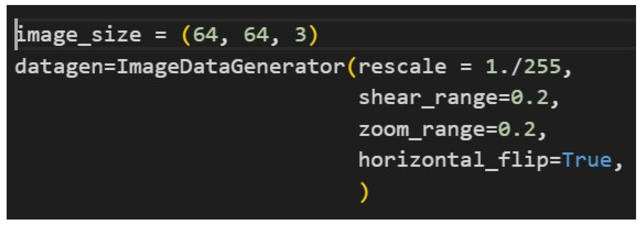
Figure 2 presents the code snippet for preparing, in Keras, an image data generator to augment image data during training. It generates images of size 64×64 pixels with three color channels and rescales the pixel values to lie between 0 and 1. Besides this, the generator applies random shearing, random zooming, and horizontal flipping to make varied versions of the same images, which is helpful to improve model generalization and reduce overfitting. This might lead to some loss of detail in the images, particularly for significant downscaling. However, the optimal size can be thought of as 64×64. Using a larger size like 512×512 may take very long to train, whereas using smaller sizes like 8×8 could result in a huge loss of detail, with the model eventually not performing well [8,9].
Figure 3.
Resized image.
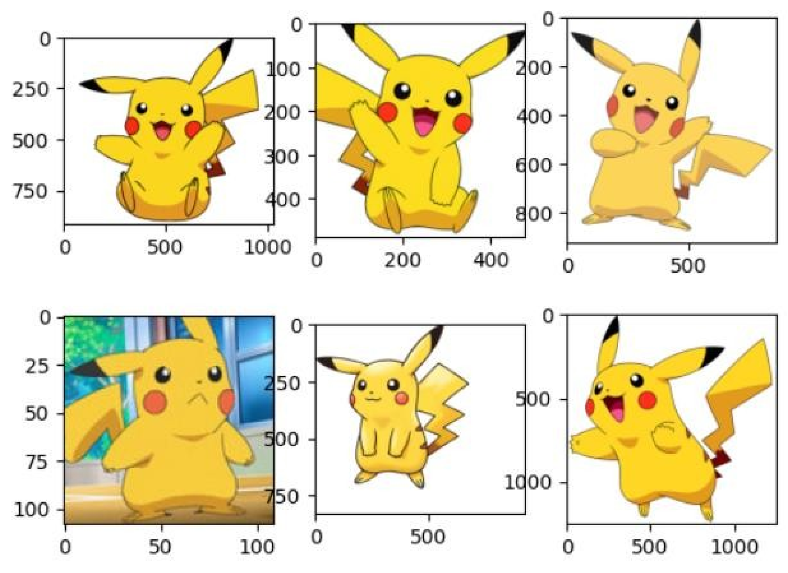
Figure 3: Six different representations of one of the most iconic Pokémon, Pikachu, after resizing, are shown here. Each of these images differs in posture, expression, and background-just the diversities needed to properly train our CNN model.
Figure 4.
Images after grey-scaling and binarizing with real image.
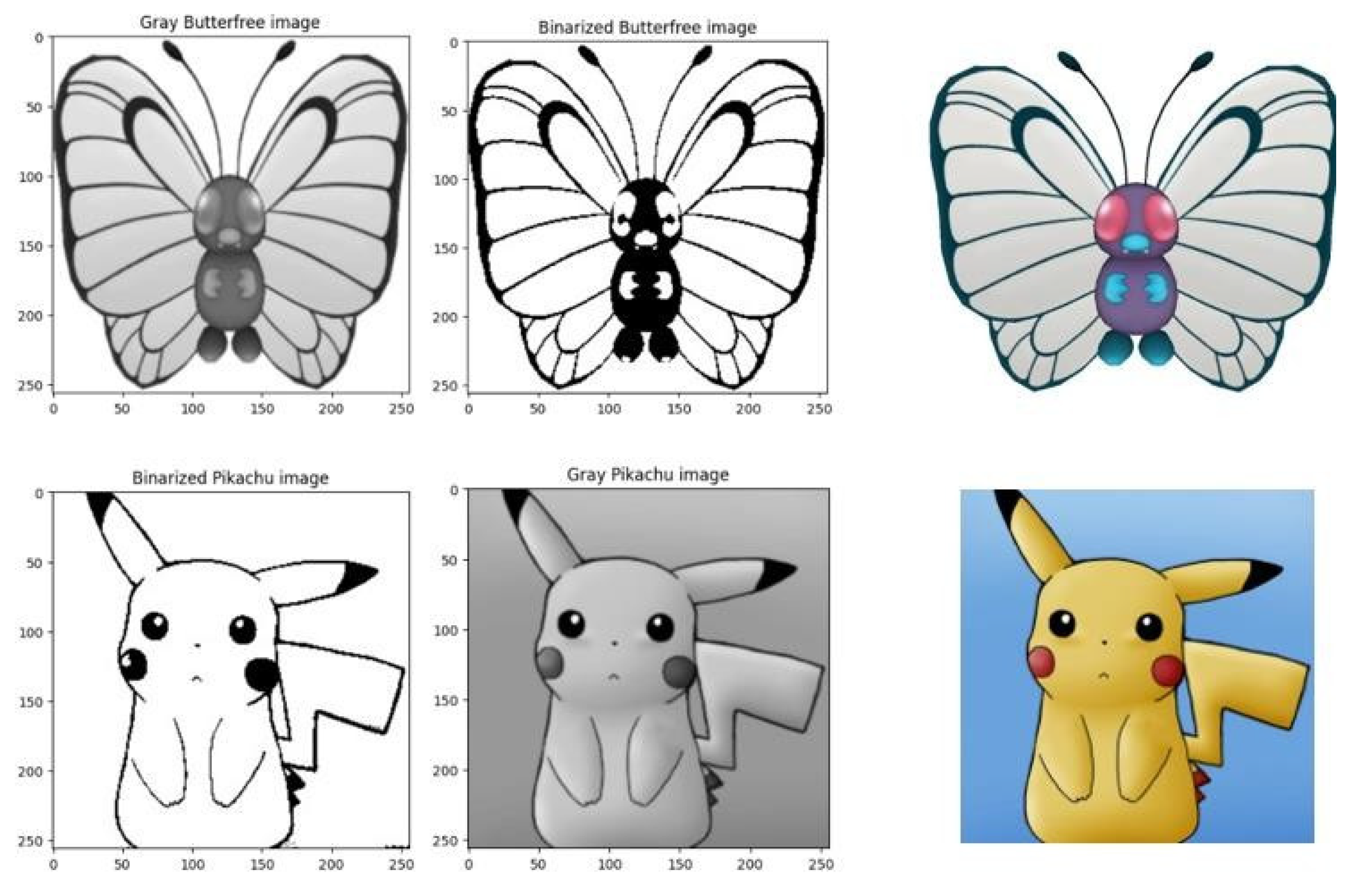
Figure 4: Grayscale, binarized, and normal versions of two Pokémon. During the preprocessing and preparation of the data, many other different methods were tried and later abandoned when desired results were not found, or other complications arose. One such approach involved first grayscale of the image and then binarizing it because it was thought at one moment that this may improve results and reduce the computational load by removing colors. This, however, did not occur since the model came out with seriously reduced accuracy; thus, this method was ultimately never used.
3. Proposed Methodology
This section reflects upon how the approach to design, implement, and evaluate the CNN model for image recognition has been done. It covers the architectural decisions [14,15] regarding the design and the technical steps required to build up and optimize the model to classify images correctly. The process was divided into sharply defined stages to eventually provide a clear-cut roadmap that will help take the model from design through implementation, considering both theoretical considerations and practical execution.
3.1. Architecture Design
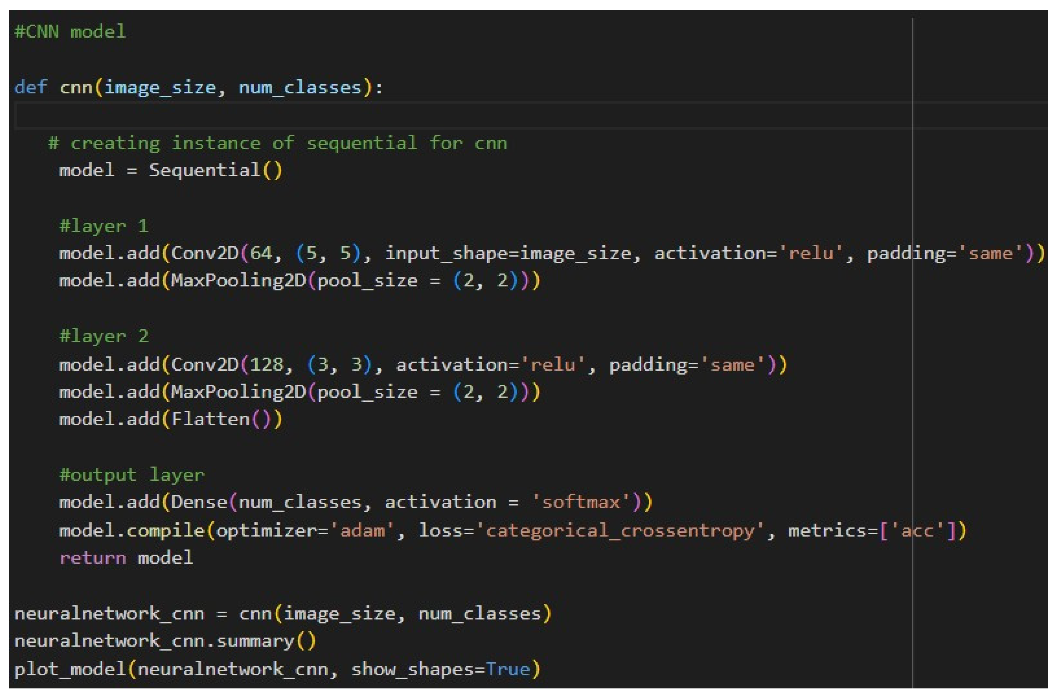
Our CNN model design takes the role of progressively extracting and refining features from input images, from a basic pattern in initial layers to abstract and complex feature detection in later layers. It contains two main convolutional layers with max-pooling to reduce dimensionality, followed by a fully connected output layer for final classification. The model is optimized using the Adam optimizer and categorical cross-entropy loss. It is designed in such a way that it performs multi-class classification with effective learning and good accuracy among the classes. The architecture of the model starts with a Conv2D layer, which takes in 64x64 RGB images, followed by a MaxPooling2D layer that reduces the spatial dimensions. This pattern is once again repeated Conv2D followed by MaxPooling2D to increase the feature extraction along with a decrease in spatial information. Further, these feature maps are flattened into a single-dimensional vector and fed in at the very end to a dense layer.
Layer 1: A Conv2D layer with 64 filters and a kernel size of (5,5) acts as a shallow feature extractor to identify some basic patterns in the input images, such as edges, lines, and shapes. This is followed by a max-pooling layer with a pool size of (2,2) that reduces spatial dimensions and, consequently, computational complexity.
Layer 2: The first layer's output is fed into another Conv2D, which has 128 filters with a kernel size of (3,3); this layer aims to find more complex patterns while another max-pooling layer reduces the dimensionality and retains features.
Output Layer: The output from the convolutional and pooling layers is fed into a fully connected Dense layer with num_classes neurons using the softmax activation function, which gives class probability distributions for effective multi-class classification.
Figure 5.
Our CNN Model Architecture.
The image Figure 6 depicts a visual representation of a Convolutional Neural Network (CNN) architecture, showing the sequential layers of the model with clear input and output shapes for each stage. The diagram starts with a Conv2D layer, which processes 64x64 RGB images, followed by a MaxPooling2D layer that reduces spatial dimensions. This pattern repeats with another Conv2D and MaxPooling2D pair, further extracting features and compressing the spatial information. The feature maps are then flattened into a single-dimensional vector, which is passed to a dense layer at the end. The flow between layers is illustrated with arrows, and each block prominently displays the input and output shapes, emphasizing the transformation of data across the model.
3.1.1. Layer 1
Layer 1 starts with a Conv2D layer that has 64 filters, each with a kernel size of (5, 5). This initial layer acts as a basic feature extractor, focusing on identifying fundamental patterns in the input images, such as edges, lines, or simple shapes. The relatively large kernel size of (5, 5) allows the network to capture more extensive spatial patterns early on, which can be particularly beneficial if the images contain more intricate or larger structures that need to be recognized. Additionally, the use of padding='same' ensures that the output feature maps retain the same spatial dimensions as the input, thus preserving important boundary information in the images. Following the convolution, there is a max-pooling layer with a pool size of (2, 2), which reduces the spatial dimensions of the feature maps by half. This pooling layer helps reduce the overall computational cost and provides a degree of translation invariance by focusing on the most prominent features.
3.1.2. Layer 2
Layer 2 builds upon the features learned in the first layer by introducing a new Conv2D layer with 128 filters and a smaller kernel size of (3, 3). By increasing the filter count, the network can capture more complex and abstract features, as each subsequent layer in a CNN generally learns more intricate patterns. The smaller kernel size in Layer 2 narrows the focus of the feature extraction process, helping the network detect finer details within the image. Like Layer 1, this layer also uses padding='same' to maintain spatial dimensions, ensuring that no valuable information is lost along the edges. Another max-pooling layer with the same pool size of (2, 2) follows, further reducing the spatial size of the feature maps while retaining the most crucial information. Finally, a Flatten () layer converts the 3D output of the second pooling layer into a 1D array, preparing the data for the fully connected layer.
3.1.3. Output Layer
The output layer is a fully connected Dense layer with num_classes neurons, where each neuron represents a possible class in the classification task. The softmax activation function is applied here to provide a probability distribution over the classes, allowing the model to output a confidence level for each class. This setup is suitable for multi-class classification tasks, as softmax is specifically designed to handle such scenarios. The model is compiled with the Adam optimizer, a widely used optimizer that adapts the learning rate during training, making it efficient for deep learning tasks. The categorical cross-entropy loss function is ideal for multiclass classification, as it measures the divergence between the predicted and actual distributions. Overall, the CNN model architecture is crafted to effectively balance feature extraction with computational efficiency, progressing from basic pattern detection to sophisticated classification. Each layer plays a distinct role in capturing essential image details and refining the model’s ability to differentiate between classes. This design supports reliable image recognition, meeting the needs of multi-class classification while accommodating the dataset's complexity.
3.2. Implementation
This is now the implementation stage, structuring, preprocessing, and training of the dataset. First, there's the division of the dataset into a training set and a test set where the training images are put in the 'Pokemon_Train' directory, and classes are represented as structured sets of empty folders in the 'Pokemon_Test' directory. The function was modified to randomly select 15 images per class from the training dataset and copy them into the test directory to create this test dataset so that the test set is unbiased. Data augmentation and preprocessing are two of the most crucial steps in any model's performance. The images here are resized, and pixel values are normalized, along with different augmentations such as random shearing, zooming, and flipping, using Keras' Image Data Generator. These transformations result in the introduction of variance in the dataset, thereby increasing the generalization capability of the model to avoid overfitting.
Figure 7 describes creating and preparing a dataset to perform Pokémon classification, structuring data organization. It first defines the working directory, 'Pokemon', which would house all classes in a total number of 150 classes. Furthermore, create a new directory named 'Pokemon_Train' and move all class folders from the main 'Pokemon' directory into 'Pokemon_Train', so that 'Pokemon_Train' will be a home for training data. Then, a 'Pokemon_Test' folder is created with a copy of all subdirectories inside 'Pokemon_Train'. That way, both folders will have exactly the same hierarchical structure, a thing that is very important for most of the libraries relying on directory organization as a basis for classifying images. Finally, all images are removed inside the 'Pokemon_Test' folder, leaving only empty folders, therefore creating a test structure with labels but no data. Both directories are assigned to variables matching their names in the last step.
Code given makes a function selecting 15 random images in every Pokémon class inside the Train directory and transfers to the right folder in each test class folder, thus arranging everything for Train-Test divisions. It's this way sure the test data contains a portion of images in the same distribution than the dataset; this represents, in actual case, more precise testing the skill of your model. The code constructs a separate test dataset with the balanced classes inside the train-test sets by looping over each class folder in the training set and performing this function. This random choice helps to avoid biased results because of a fixed test set and keeps the model from getting over-fitted by seeing a wide range of test data. The generalizing capability of the model, along with its robustness, improves in this process.
Figure 9 shows how the ImageDataGenerator class from Keras is used to load, preprocess, and batch images from specified directories and prepare them for training and validation. The first snippet defines a training set generator by calling the function datagen.flow_from_directory(train_dir). The generator targets the train_dir, which should contain subdirectories named according to the categories in the training dataset. Each subdirectory is supposed to hold pictures for one class in general. For example, "cats" or "dogs" in a classifier able to recognize animal types. A configuration like this will ensure that the model will learn from labelled data [19,20,21].
In this target_size= image_size[:2], it's indicated that all images will be resized to 'uniform width and height' from the image_size variable. This just slices out the first two dimensions, disregarding any channel information so that these could be made uniform across the dataset for the input layer of the CNN. The batch_size = 32 parameter sets the number of images to process in a single batch-a trade-off between computational efficiency and memory consumption because batches are processed sequentially during training [16,17,18]. Finally, class_mode = 'categorical' states that the labels are categorical and automatically one-hot-encodes them, which is useful if using categorical cross-entropy as a loss function. Lastly, color_mode = 'rgb' ensures that images are loaded in full color-three channels for red, and green, and blue-which is important for models that rely on color information for classification. The second snippet is to create a validation_set generator, which, similarly in structure, points to test_dir instead of train_dir. In this folder are the validation images, arranged like in the training directory, with class-named subfolders. The images for validation determine how well the model generalizes on unseen data; thus, enabling the detection of overfitting that may occur. This class takes target_size, batch_size, class_mode, and color_mode identical to the ones used in the creation of training_set, ensuring that both datasets are uniformly processed.
These steps were essential to be done before the execution of the model. However, since the model execution process is already explained in the Architecture Overview, the discussion hereafter will be done on the steps performed post running the model [22,23,24,25].
Figure 10 shows the code for the training process of the constructed model, which is trained through the fit method. It took in the training set as input and the validation set as validation data to monitor model performance. To optimize, manage, and control the training process, several callback functions were created: 'es' for early stopping, 'ckpt' for saving model checkpoints, and 'rlp' for reducing the learning rate in case of no further improvement. These callbacks will enhance training efficiency and help avoid overfitting by stopping the training when it stops improving, while it saves the best model and dynamically adjusts the learning rate. The model is trained up to a limit of 20 epochs, but if the early stop criteria are fulfilled, training could stop earlier. The limit has been set as 20 to strike a fine balance in terms of training time, ensuring effectiveness in learning from the model but not overfitting. Details concerning metrics both on training and validation across all epochs are captured in the history object returned by the fit method, which can be used later for performance analysis and visualization.
Figure 11 presents the result of running 20 epochs. It would be too time-consuming to paste the output of all 20 runs here, so only the results of the last few runs are shown. From these, one can see that the model is still improving in accuracy. As was mentioned before, 20 runs should give a good balance: The model learned from most of the dataset and will not overfit.
4. Results and Discussion
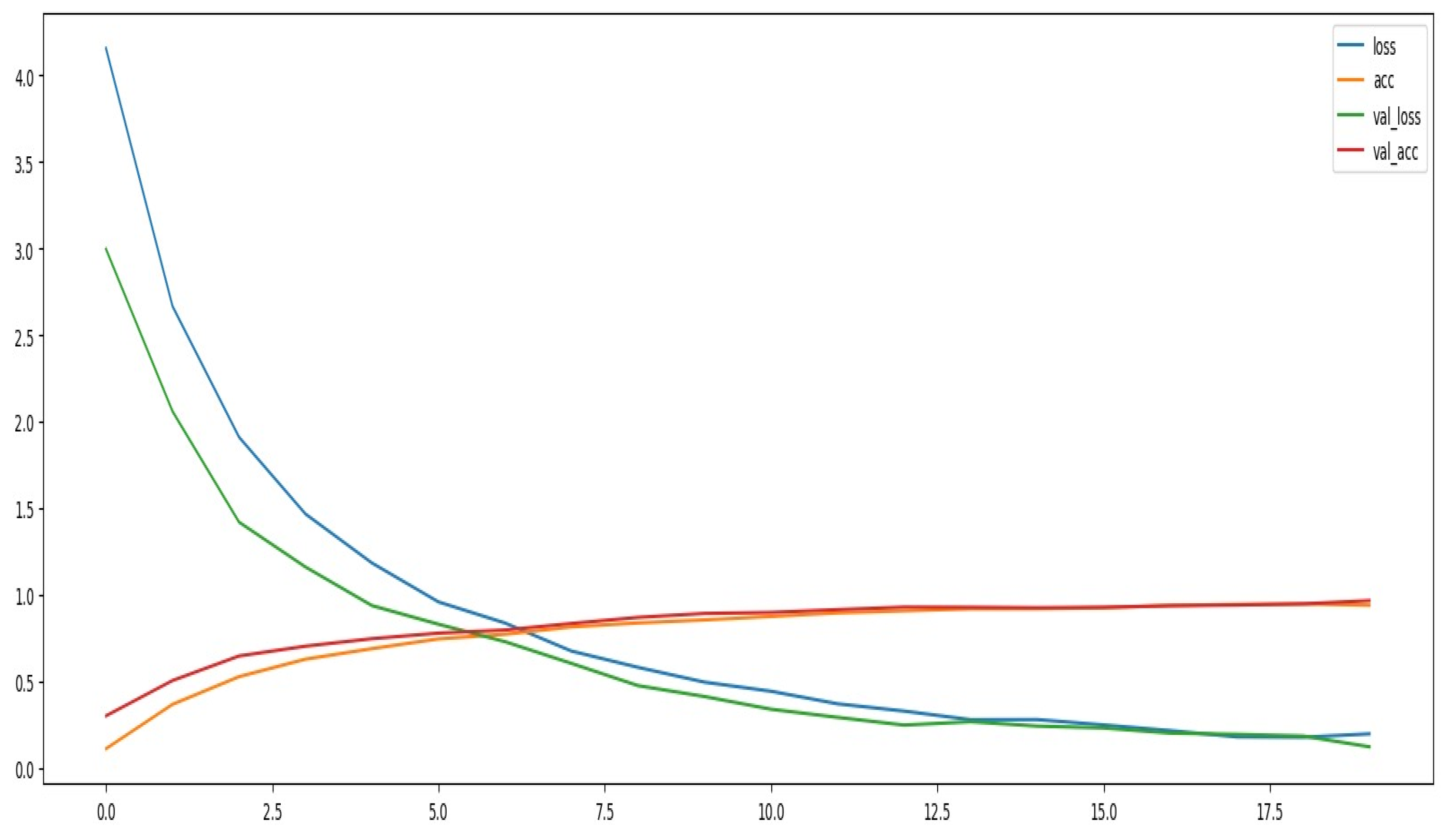
A performance evaluation is done by analyzing different metrics of the CNN model for Pokémon classification, including accuracy, precision, recall, and F1-score. It points out how the model learns the pattern and generalizes from the dataset. Figure 12 represents a Comparison of training versus validation accuracy over various epochs. The training and validation accuracies increase sharply for the first epochs, which already suggests that it learns well from the data and generalizes nicely to unseen ones. This fact at least points out that a CNN model was able to make something meaningful from the dataset. Moreover, relatively close alignment in training and validation accuracy curves for the beginning period of training at least suggests there is no severe overfitting of the model.
With progression in training, the training accuracy increases closer to its optimal value, while the validation accuracy soon starts to degrade and reaches a point where there is a crossing of the two curves. This suggests that overfitting becomes slightly worse by memorizing certain features in training rather than general features across new data, yet the accuracy remains quite good, inferring a good balanced learning process with not much overfitting.
Model Performance Metrics
Figure 13: The classification model of the Pokémon had a very good accuracy of 95.8%. With such a high accuracy score, it is confirmed that the CNN can distinguish between 150 species of Pokémon with considerable precision and recall. Besides, Figure 14 presents precision, recall, and F1-score metrics that corroborate balanced performance across different classes:
| Metric | Score |
| Macro-Average | 0.96 |
| Weighted Average | 0.96 |
These results confirm that the model does not favor any particular class disproportionately, hence it is well-calibrated regarding classification. A balance between precision and recall suggests that the model effectively minimizes false positives and false negatives, hence highly reliable for real-world applications where accurate classification is essential. Figures 15 and 16 show the integration of the trained CNN model into a user-friendly interface. A working 'Upload Button' and a 'Predict Button' to upload an image of a Pokémon and get the prediction across the model. Figure 16: In the case of a random image of Pokémon that was uploaded, the model rightly predicted it as 'Aerodactyl.' This shows that this model will work in the real world for classifying Pokémon, thus useful in practice. The classification of Pokémon through CNN has resulted very well, while its accuracy, precision, recall, and F1-score are relatively high out of 150 classes. From the learning curves, it can be observed that generalization was pretty effective, with minor overfitting toward the end of training. Thus, deploying the model onto an interactive interface proves its usability, and it can be considered a strong Pokémon classification model. Future work may apply more generalization techniques, such as data augmentation and regularization, that prevent overfitting and further improve performance.
5. Conclusion
This research work focused on CNN-based Pokémon classification, resulting in an overall 95.8% test accuracy, and generally good precision and recall across classes. The findings also emphasize the model's ability to capture very minute nuances between species, reflecting the robustness of the CNN design itself, along with the efficacy of the preprocessing and data-handling strategies that were put into practice. Balanced on different classes suggests that this might perform very well on other similar classification tasks, with very close similarities among the classes. It is a good model and, with improvements of hyperparameters along with better regularization, avoiding the slight overfitting towards the end epoch, the result might reach closer to reality with higher accuracy. However, for this project, it stays beyond the scope of interest. This work represents valuable insight into the optimization of CNN for image classification and provides the base for any future work on fine-grained and large-scale classification problems.
References
- Anjli, V., & Malathy, J. A. P. (2023). A study on deep learning models for automatic species identification from novel leather images. Proceedings of the International Conference on Artificial Intelligence and Communications Technology (IAICT). [CrossRef]
- Balarabe, A. T., & Jordanov, I. (2024). A deeper look into remote sensing scene image misclassification by CNNs. IEEE Access.
- Haffar, R., Jebreel, N. M., Domingo-Ferrer, J., & Sánchez, D. (2021, September). Explaining image misclassification in deep learning via adversarial examples. In International Conference on Modeling Decisions for Artificial Intelligence (pp. 323-334). Springer International Publishing.
- Hu, C., Sapkota, B. B., Thomasson, J. A., & Bagavathiannan, M. V. (2021). Influence of image quality and light consistency on the performance of convolutional neural networks for weed mapping. Remote Sensing, 13(11), 2140.
- Inzamam, U. H., Dubey, A. K., Danciu, I., Justice, A. C., Ovchinnikova, O. S., & Hinkle, J. (2023). Effect of image resolution on automated classification of chest X-rays. Journal of Medical Imaging, 10(4), 044503. [CrossRef]
- Mo, H., & Wei, L. (2024). SA-ConvNeXt: A hybrid approach for flower image classification using selective attention mechanism. Mathematics, 12(14), 2151.
- Surve, Y., Pudari, K., Bedade, S., Masanam, B. D., Bhalerao, K., & Mhatre, P. (2024, April). Comparative analysis of various CNN architectures in recognizing objects in a classification system. In 2024 IEEE 9th International Conference for Convergence in Technology (I2CT) (pp. 1-5). IEEE.
- Zhao, Z. (2023). The effect of input size on the accuracy of a convolutional neural network performing brain tumor detection. Proceedings of SPIE - The International Society for Optical Engineering. [CrossRef]
- Dataset:Lantian773030. (n.d.). Pokémon classification dataset. Kaggle. Retrieved from https://www.kaggle.com/datasets/lantian773030/pokemonclassification.
- Dogra, V., Singh, A., Verma, S., Kavita, Jhanjhi, N. Z., & Talib, M. N. (2021). Analyzing DistilBERT for sentiment classification of banking financial news. In S. L. Peng, S. Y. Hsieh, S. Gopalakrishnan, & B. Duraisamy (Eds.), Intelligent computing and innovation on data science (Vol. 248, pp. 665-675). Springer. [CrossRef]
- Gopi, R., Sathiyamoorthi, V., Selvakumar, S., et al. (2022). Enhanced method of ANN based model for detection of DDoS attacks on multimedia Internet of Things. Multimedia Tools and Applications, 81(36), 26739-26757. [CrossRef]
- Chesti, I. A., Humayun, M., Sama, N. U., & Jhanjhi, N. Z. (2020, October). Evolution, mitigation, and prevention of ransomware. In 2020 2nd International Conference on Computer and Information Sciences (ICCIS) (pp. 1-6). IEEE.
- Alkinani, M. H., Almazroi, A. A., Jhanjhi, N. Z., & Khan, N. A. (2021). 5G and IoT based reporting and accident detection (RAD) system to deliver first aid box using unmanned aerial vehicle. Sensors, 21(20), 6905.
- Babbar, H., Rani, S., Masud, M., Verma, S., Anand, D., & Jhanjhi, N. (2021). Load balancing algorithm for migrating switches in software-defined vehicular networks. Computational Materials and Continua, 67(1), 1301-1316.
- Kumar, T., Pandey, B., Mussavi, S. H. A., & Zaman, N. (2015). CTHS based energy efficient thermal aware image ALU design on FPGA. Wireless Personal Communications, 85, 671-696.
- Fatima-tuz-Zahra, N. Jhanjhi, S. N. Brohi, N. A. Malik and M. Humayun, "Proposing a Hybrid RPL Protocol for Rank and Wormhole Attack Mitigation using Machine Learning," 2020 2nd International Conference on Computer and Information Sciences (ICCIS), Sakaka, Saudi Arabia, 2020, pp. 1-6, . [CrossRef]
- Lim, M., Abdullah, A., Jhanjhi, N. Z., Khan, M. K., & Supramaniam, M. (2019). Link prediction in time-evolving criminal network with deep reinforcement learning technique. IEEE Access, 7, 184797-184807.
- Zaman, N., Low, T. J., & Alghamdi, T. (2014, February). Energy efficient routing protocol for wireless sensor network. In 16th international conference on advanced communication technology (pp. 808-814). IEEE.
- Kok, S. H., Abdullah, A., Jhanjhi, N. Z., & Supramaniam, M. (2019). A review of intrusion detection system using machine learning approach. International Journal of Engineering Research and Technology, 12(1), 8-15.
- Alex, S. A., Jhanjhi, N. Z., Humayun, M., Ibrahim, A. O., & Abulfaraj, A. W. (2022). Deep LSTM model for diabetes prediction with class balancing by SMOTE. Electronics, 11(17), 2737.
- Alferidah, D. K., & Jhanjhi, N. Z. (2020, October). Cybersecurity impact over bigdata and iot growth. In 2020 International Conference on Computational Intelligence (ICCI) (pp. 103-108). IEEE.
- Babbar, H., Rani, S., Masud, M., Verma, S., Anand, D., & Jhanjhi, N. (2021). Load balancing algorithm for migrating switches in software-defined vehicular networks. Comput. Mater. Contin, 67(1), 1301-1316.
- Jhanjhi, N. Z., Humayun, M., & Almuayqil, S. N. (2021). Cyber security and privacy issues in industrial internet of things. Computer Systems Science & Engineering, 37(3).
- Jena, K. K., Bhoi, S. K., Malik, T. K., Sahoo, K. S., Jhanjhi, N. Z., Bhatia, S., & Amsaad, F. (2022). E-learning course recommender system using collaborative filtering models. Electronics, 12(1), 157.
- Aherwadi, N., Mittal, U., Singla, J., Jhanjhi, N. Z., Yassine, A., & Hossain, M. S. (2022). Prediction of fruit maturity, quality, and its life using deep learning algorithms. Electronics, 11(24), 4100.
Figure 1.
Image Size.
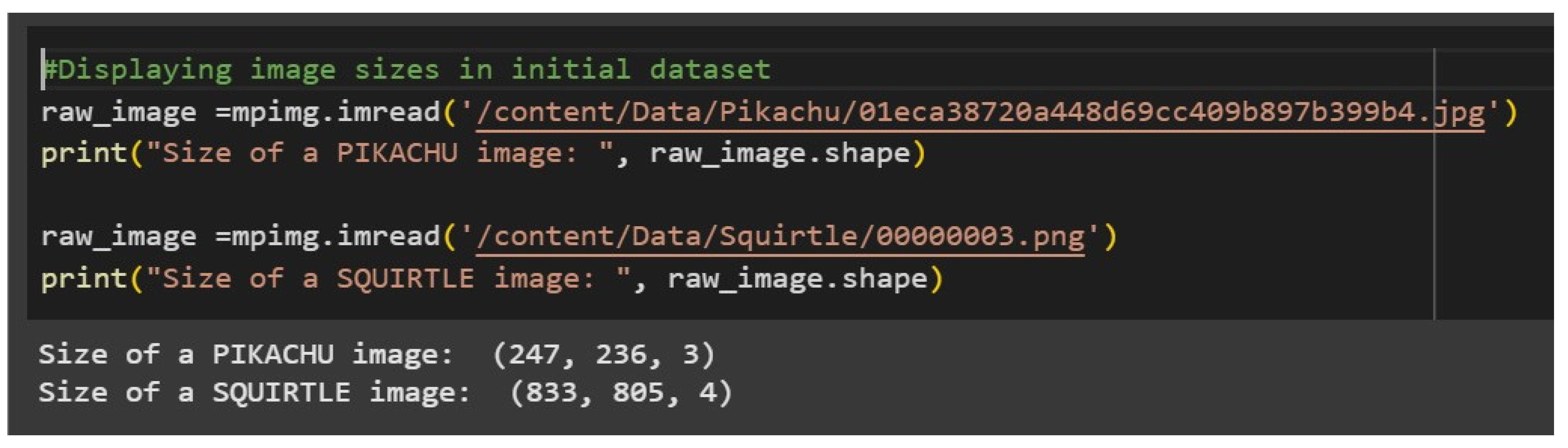
Figure 6.
Depicts a visual representation of a Convolutional Neural Network (CNN) architecture.
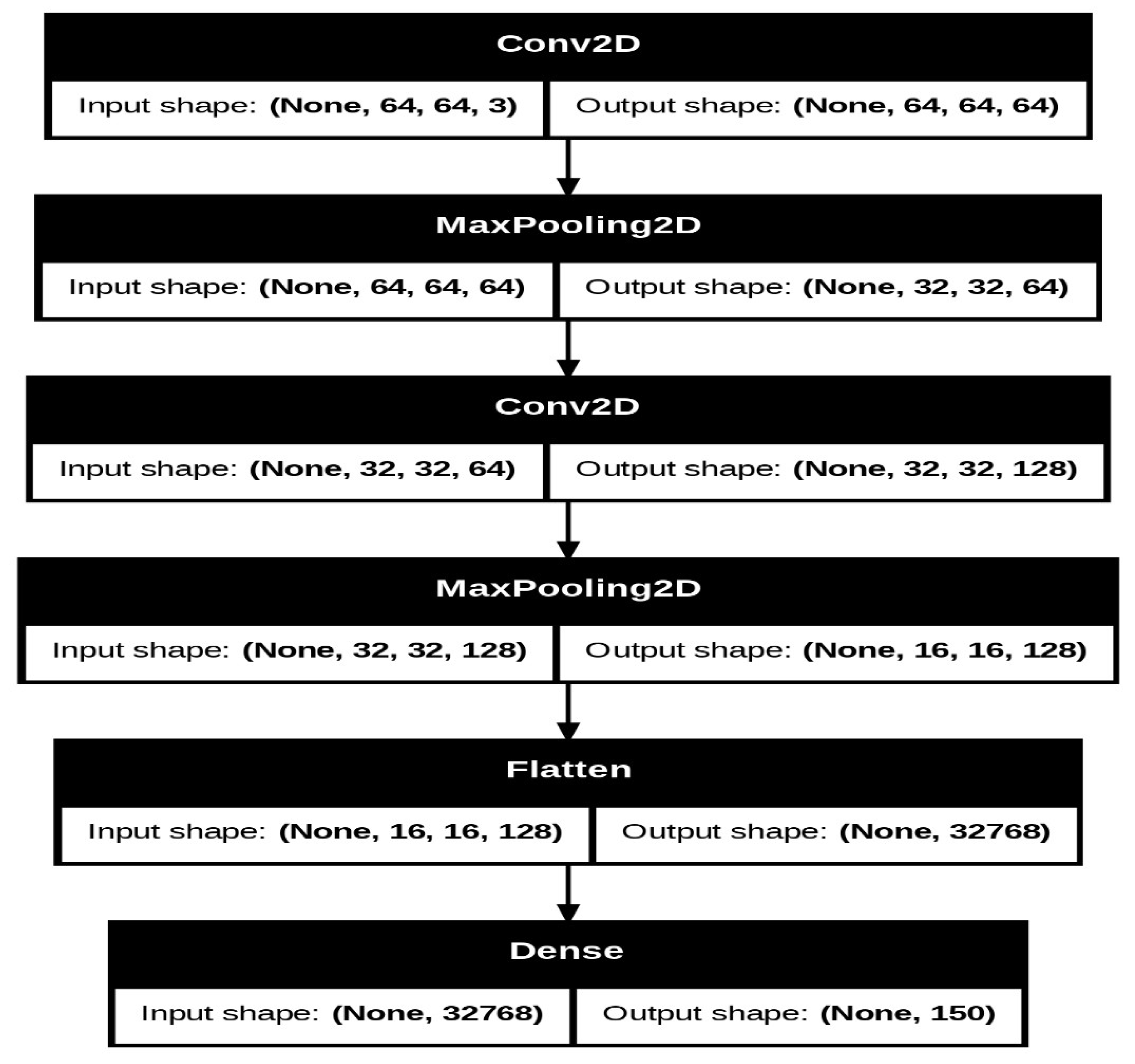
Figure 7.
Model Testing and Training .
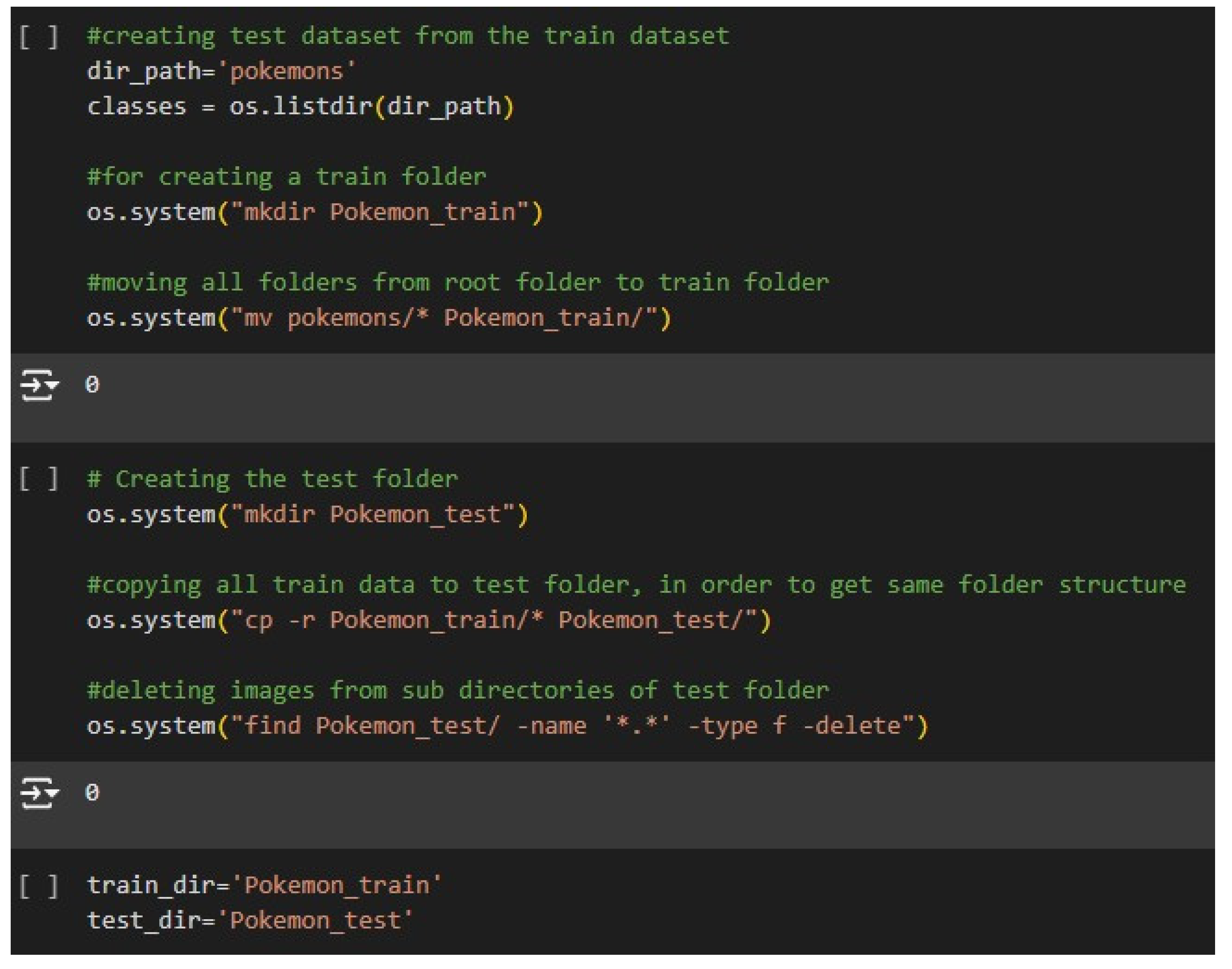
Figure 8.
Making of Testing Dataset.
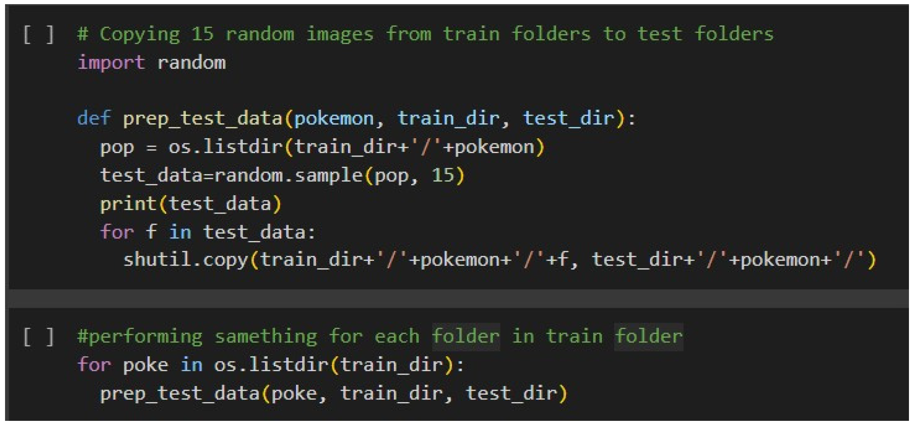
Figure 9.
Loading, Preprocessing and Batching of Images.
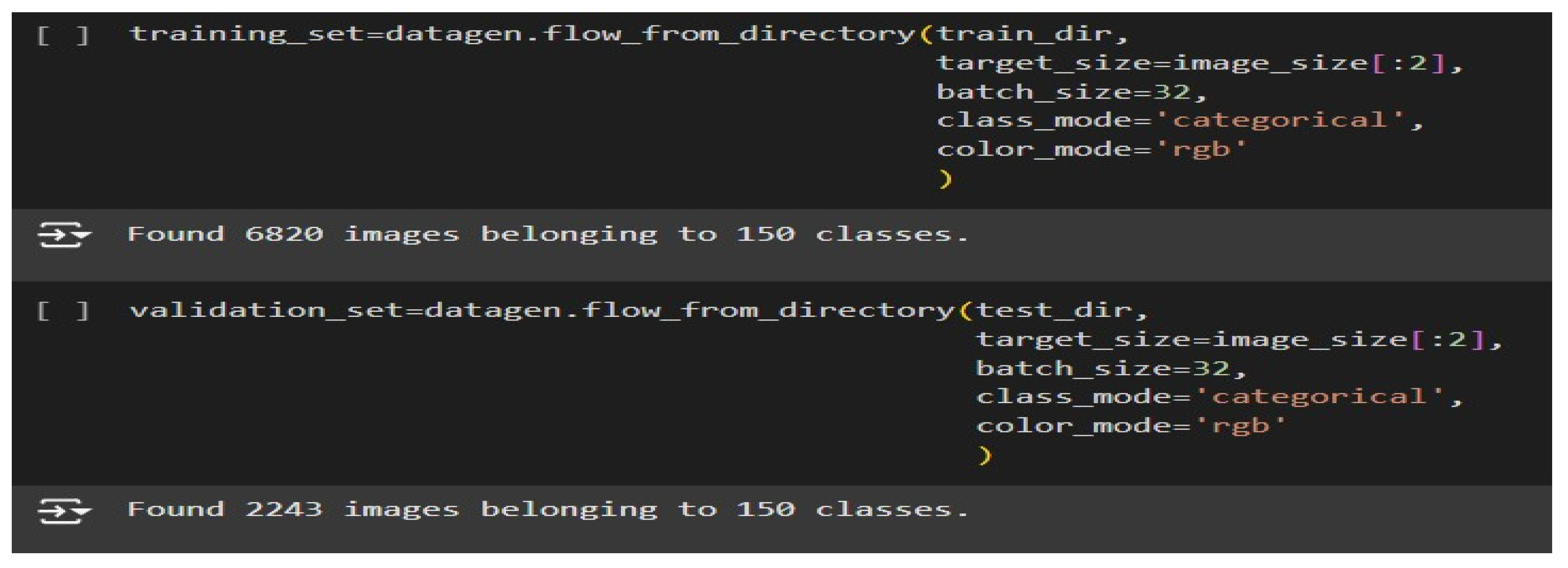
Figure 10.
Model Training.
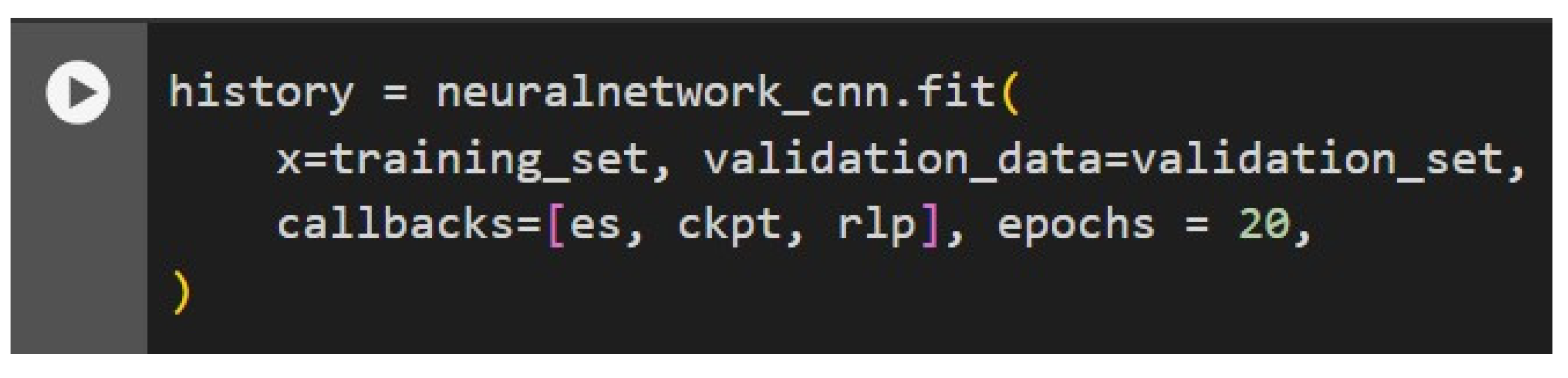
Figure 11.
Epochs.
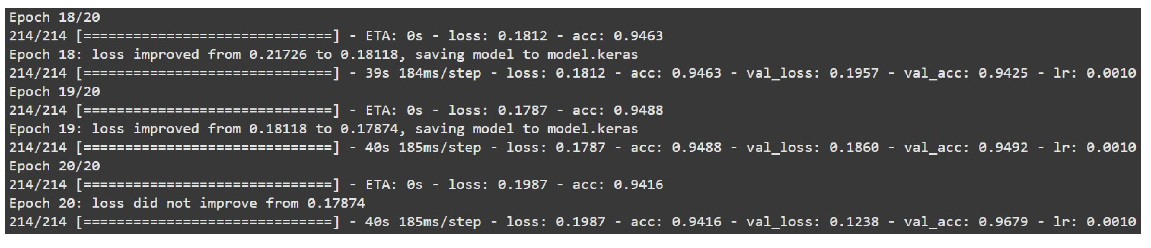
Figure 12.
Model Loss and Accuracies.
Disclaimer/Publisher’s Note: The statements, opinions and data contained in all publications are solely those of the individual author(s) and contributor(s) and not of MDPI and/or the editor(s). MDPI and/or the editor(s) disclaim responsibility for any injury to people or property resulting from any ideas, methods, instructions or products referred to in the content. |
© 2025 by the authors. Licensee MDPI, Basel, Switzerland. This article is an open access article distributed under the terms and conditions of the Creative Commons Attribution (CC BY) license (http://creativecommons.org/licenses/by/4.0/).
Copyright: This open access article is published under a Creative Commons CC BY 4.0 license, which permit the free download, distribution, and reuse, provided that the author and preprint are cited in any reuse.


