1. Introduction
A decade ago the author [1] (under influence of Odake and Sasaki’s celebrated paper [2] and its extension in [3]) demonstrated the existence of the three isospectral families of the rational
SUSY partners of the hyperbolic Pöschl-Teller (h-PT) potential [4] quantized by the rational Darboux transforms () of the Romanovski-Jacobi (R-Jacobi) polynomials [5–7] . In all the cases (labeled,, and below for the reasons specified later) the
quasi-rational transformation functions (q-RTFs) were represented by the
principal Frobenius solutions (PFSs) of the Jacobi-reference (JRef) canonical
Sturm-Liouville equation (CSLE) nonvanishing in the quantization interval
(+1,∞). The finite exceptional orthogonal polynomial EOP sequence reported in [3] was identified by us as type. As pointed to in [8] ,
the infinitely many finite polynomial sequences of typewere constructed by Grandati [9] a year earlier; however, he did not recognized
the fact that, in contrast with other potentials discussed in the paper, the
aforementioned polynomial sequences are X-orthogonal with a positive weight.
In the same year as [1] ,
Yadav et al. [10] calculated the scattering
amplitude for the rationally extended h-PT potential solvable by the
finite sequence of the EOPs of type , referring to the latter simply as ‘Xm-Jacobi
EOPs’. The epithet (repeatedly used by these authors in the more recent papers [11–14] ) seemed confusing since the EOPs in question
do not belong to the Xm-Jacobi orthogonal polynomial system (OPS) [15–17] and therefore cannot form its finite subset.
Before continuing our discussion, let us first
point to the dubious use of the term ‘EOP’ in the literature, similar to the
slang use of the term ‘orthogonal Jacobi polynomials’, instead of ‘classical
Jacobi polynomials’, which disregards the existence of the finite orthogonal
subsets formed by the R-Jacobi polynomials. Similarly, Gȯmez-Ullate, Milson et al. [15,16,18,19]
use the term ‘EOPs’ as the synonym for ‘X-OPS’, disregarding the existence of
the finite EOP sequences [1–3,8,10–13,20–30]
represented by the rational Darboux transforms () of Romanovski polynomials [1,8,21,24–29] . (As a puzzling exception, Gȯmez-Ullate, Grandati, and Milson [31] , when citing the studies on the EOPs, did
mention the papers [9] and [20] , which deal solely with the problems solved by
the finite EOP sequences.)
On the other hand, Yadav et al. in their progressed
study [11] on the rational extensions of the h-PT
potential used the term ‘EOP’ in both ways: they first identified the families of
EOPs as ‘Xm-Laguerre and Xm- Jacobi polynomials’
(apparently implying the Xm-Laguerre and Xm- Jacobi OPSs)
but then presented the long list of the papers dealing with both infinite and
finite EOP sequences. The cited authors then discussed the quasi-rational
eigenfunctions of the rationally extended h-PT and Scarf I potentials,
referring to their (finitely and respectively infinitely many) polynomial
components as ‘EOPs’. Yadav et al took later more cautious approach [12] , first mentioning the three pioneering studies [15,32,33] on the Xm-Jacobi and Xm-
Laguerre OPSs and then citing a mixture of papers which discussed both infinite
and finite EOP sequences. (Regrettably, their later paper [12] overlooked our analysis [8,24] cautiously distinguishing between the Xm-
Jacobi OPSs and finite EOP sequences formed by theof the R-Jacobi polynomials.)
The rigorous analysis of the aforementioned finite
EOP sequences of types ,, andin [24] revealed
that the EOP sequences of typesandare formally generated by the same shift operators
as the cases J1 and J2 case in [3] , except
that the indexes of the seed Jacobi polynomials in our case were independent of
the polynomial degrees. This observation brought the author [24] to the concept of the exceptional differential
polynomial systems (X-DPSs), with the term ‘DPS’ used in exactly the same sense
as it was suggested by Everitt et al. [34,35]
for conventional sequences of polynomials obeying the Bochner theorem [36] . In following the commonly accepted terminology
suggested by Gȯmez-Ullate et
al. [33] for the X1 -OPSs, we call the given DPS exceptional because the
polynomial sequence in question either does not start from a constant or lacks
the first-degree polynomial and therefore do not obey the Bochner theorem.
Indeed, as stressed by Kwon and Littlewood [37] ,
Bochner himself “did not mention the orthogonality of the polynomial systems
that he found. The problem of classifying all classical orthogonal polynomials
was handled by many authors thereafter” based on his analysis of possible
polynomial solutions of complex second-order differential
eigenequations.
Compared with the rigorous mathematical analysis of
the X-OPSs in [18,19] , the concept of the
X-DPSs put forward by us in [24] represents
the parallel direction dealing with the solvable rational CSLEs (RCSLEs) and
related X-Bochner ordinary differential equations (ODEs), instead of the (irregular)
exceptional Bochner (X-Bochner) operators in [18]
and related polynomial Sturm-Liouville problems (PSLPs) sketched in [15,18,32] .
The interrelation between the two approaches is
closely related to the dual use of the term ’Darboux transformation’ (DT),
following the discovery by Andrianov et al [38,39]
that the renowned transformation of the Schrödinger equation initially
suggested by Darboux [40] for the generic
second-order canonical differential eigenequation (long before the birth of the
quantum mechanics) is equivalent to its intertwining factorization. We refer the reader to the excellent overview of this
issue in [41] .
More recently Gȯmez-Ullate
et al. [42] initiated the new direction in the
theory of the rational Sturm-Liouville equations (RSLEs) by applying the
intertwining factorization to the second-order differential eigenoperator. This
operation was termed ’Darboux transformation’, based on the dualism existent in
the particular case of the Schrödinger operator. This innovation followed by
its extension to the X-OPSs [15,32,33] laid
the foundation for their rigorous theory advanced to the higher level in [18,19] .
The author (being accustomed [43] to the strict use of the mentioned term) took
the different turn [1] in the extension of the
DTs to the SLEs. As we understand now, our original intuitive idea was based on
the three-step operation:
- i)
the Liouville transformation from the CSLE to the Schrödinger equation;
- ii)
the Darboux deformation of the corresponding Liouville potential;
- iii)
the reverse Liouville transformation from the Schrödinger equation to the new CSLE using the same change of variable as at Step i).
referred to by us years later [44] as ‘Liouville-Darboux transformation’. Note
that we invented the term ‘Darboux deformation’ (DD), used instead of ‘DT’,
simply to avoid the multiple repetition of the word ‘transformation’. It is
worth stressing again that we give to this term its original meaning implied by
Darboux [40] .
The extensive exploration of the literature
revealed that the transformation of the CSLE sketched above has been introduced
by Rudyak and Zakhariev [45] in the late
eighties. Schnizer and Leeb [46,47] named it ‘generalized
Darboux transformation’ (GDT); this name was also accepted in some later
studies on this subject. However, since various authors give to this widely
used name completely different meanings in both physics and mathematics (see [44] for numerous examples), we suggested the
aforementioned name ‘Liouville Darboux transformation’ as an alternative. Our
current perception is that the latter is slightly misleading because it relates
the definition of the transformation to the DD of the Liouville potential,
which is absolutely irrelevant to the problem under consideration unless we are
interested in quantum-mechanical applications.
Below we simply refer to the GDTs in question as
‘Rudjak-Zakhariev transformations’ (RZTs) and consider its three-step
decomposition suggested in [44] just as one of its realizations, but not as its definition (see Appendix A for more details). We term the RZT of the RCSLE as ‘rational RZT’ (RRZT) if it uses a q-RTF.
In this paper we, based on the results of our
previous studies [8,24] , scrupulously analyze
the manifold of the RCSLEs obtained by RRZTs of the Jacobi-reference (JRef)
CSLE which is defined defined via (1)-(3) in Section
2 . Each quasi-rational solution (q-RS) formed by a m-degree Jacobi
polynomial can be used as the q-RTF giving rise to the RCSLE with m+2 poles in
the finite complex plane. The Jacobi indexes of the seed polynomials are
defined in the segments carved by the three vertical and three horizontal lines
with the abscissas and respectively ordinates equal to -1, 0, and +1.
Each transformed CSLE is then converted to the Bochner-type
ODE with polynomial coefficients, taking advantage of the fact that the density
function of our interest has only simple poles in the finite plane and as a
results the mentioned gauge transformation is energy-independent [1] . Concequently, the linear coeficient function of
the resultant differential equation does not depend on degrees of the
sought-for polynomials.
It has been proven in [24]
that each transformed RCSLE constructed in such a way has a quartet of infinite
sequences of q-RSs with polynomial components forming the four Xm-Jacobi
DPSs of series J1, J2, D, and W, as they were termed by us. The shift operators
for the cases J1 and J2 in [3] match our
equations for the Xm-Jacobi DPSs of series J1 and J2 accordingly,
though, as pointed to in [8] , the indexes of
the seed Jacobi polynomials in our scheme are independent of the polynomials,
in a sharp contrast with [3] .
The most important part of our formalism is to
formulate the rational Sturm-Liouville problem (RSLP) to find all infinite or
finite orthogonal subsequences in each of the four Xm-Jacobi DPSs.
Note that, until now, we have not imposed any restriction on the zeros of the
seed Jacobi polynomials. However, to select the RSLPs solvable by either
infinite or finite EOP sequences, we have to focus solely on the seed Jacobi
polynomials with no zeros inside the quantization interval. At this point we
come to the main advantage of our approach, compared with the general theory of
X-OPSs advanced by Garcia-Ferrero
et al. [18,19] . Namely we
formulate the RSLP for both finite and infinite quantization intervals whereas
the Xm-Jacobi OPSs appear only if the OBCs for the given SLP are
imposed at the ends of the finite interval (-1,+1). Since the cited authors
were interested only in the X-OPSs they term the X-Bochner operator ‘regular’,
if the q-RTF used to generate the RCSLE in question does not have nodes inside
the interval (-1,+1). On the contrary, we have to additionally specify the open
interval, where the RCSLE of our interest may not have any singularities. For
the purposes of this paper (unless explicitly specified otherwise) the q-RTF is
termed regular if does not have real nodes larger than 1. Similarly we refer to
the RRZT as regular (reg-RRZT) if the corresponding transform of the
JRef CSLE does not have poles in the interval (1,∞).
A certain deficiency of our Sturm-Liouville
approach, compared with the intertwining technique advanced in [18,19] , is that we [48]
require that the RRZT of the RSLE preserves both the leading and weight
coefficient functions. As a result, the RRZTs, as they define here, represent
only a narrow subset of the rational Darboux transformations (RDTs) in the
terminology of Garcia-Ferrero
et al. [18,19] .
As
it has been already done above in our references to the of the Romanovsky polynomials, we will often use
the commonly accepted term ‘’, instead of ‘’, despite the more restrictive requirement for
both indexes of the classical Jacobi polynomial or the first index of the
R-Jacobi polynomial to be positive.
Our next step is to find all quasi-raional solutions
(q-RSs) of the JRef CSLE, which do not have nodes inside the selected
quantization interval, which assures that the transformed RCSLE does not have
poles inside the interval of our interest. It was taken for granted in our
earlier works [1,8,24] that any PFS below the
lowest eigenvalue is necessarily nodeless. As one can see from the proof
presented in Appendix B , this is not by
any means a trivial (though wide-spread) presumption.
Using Klein’s formulas (see §6.72 in [49] ) for the numbers of zeros of a Jacobi
polynomial in the intervals (-∞,-1), (-1,+1), and (+1,∞), we showed [1] that the JRef CSLE also has q-RSs of type with no nodes in the interval (+1,∞). Keeping in
mind the RRZT using this q-RS as q-RTF inserts the extra energy level below the
lowest eigenvalue, it can be called [41]
‘dressing’ transformation.
To find all the orthogonal of the classical and R-Jacobi polynomials, we
convert the transformed RCSLE to its prime form defined in such a way [48] that the Dirichlet boundary condition (DBC)
unambiguously selects the PFS near the singular end in question. As a result,
the DBCs at the ends of the given quantization interval select the solutions
representing the PFSs near both singular ends.
In the limit point (LP) region this procedure unequivocally
specifies the eigenfunctions square integrable (by definition) with the weight
function in the SLE under consideration. Our procedure also provides the
prescription for constructing EOP sequence in the limit circle (LC) region,
where the corresponding Liouville potential has only continuously degenerate
bound energy states (CDBESs).
We found that the Xm-Jacobi DPSs of both
series J1 and J2 contain Xm-Jacobi OPSs, which are interrelated via
the reflection of their argument accompanied by the interchange of the Jacobi
indexes. For this reason Gȯmez-Ullate
et al. [15,16] focused solely on the
properties of one of them (which happened to be the Xm-Jacobi OPS of
series J2 in our terms), referring to the latter simply as the Xm-Jacobi
OPS and dropping the Xm-Jacobi OPS of series J1 from any future
consideration.
On other hand, our analysis revealed that the
infinitely many finite EOP sequences of type and limitedly many the finite EOP sequences of type(constructed using the PFSs near the origin and at
infinity respectively) belong to the Xm-Jacobi DPS of series J1 and
accordingly J2, which makes it necessary to analyze both X-DPSs in parallel.
In particular, as discussed in subsection 4.2
below, the Xm-Jacobi DPS of series J2 contains the Xm-Jacobi
OPS (in terms of [15,16] ), the finite EOP
sequence orthogonal on the negative interval (-∞,-1), and another finite EOP
sequence orthogonal on the positive interval (1,∞). The latter EOP sequence of
typeis composed theof the R-Jacobi polynomials which represent the
polynomial components of the eigenfunctions [10–12]
of the rationally extended h-PT potentials [11,12] .
Regretfully, both our works [8] and [24]
overlooked the important modification in the definition of the ‘Xm-Jacobi
polynomials’ by Yadav et al. in [11] . Namely
the indexes α and β appearing in the expression
for Xm-Jacobi polynomials’ in [10]
were defined independently of the degree of the seed Jacobi polynomials and
thereby (as illuminated in subsection 4.2 below) made the mentioned expression
fully consistent with our definition of the Xm-Jacobi DPS of series
J2.
As for the Xm-Jacobi DPS of series J1,
it contains the OPS (‘Xm-Jacobi OPS of series J1 in our terms), the
finite EOP sequence orthogonal on the negative interval (-∞,-1), and another
finite EOP sequence (this time of type) orthogonal on the positive interval (1,∞).
Obviously, the finite EOP sequence orthogonal on the negative interval (-∞,-1)
can be obtained from the EOP sequence of type by the reflection of the argument, followed by the
interchange of the indexes; i.e., the two finite EOP sequences in question are
interrelated in exactly the same way as the DPSs of series J1 and J2 to which
they belong.
The third EOP sequence of type generated using the PFSs near origin (similarly to
EOP sequence of type ) constitutes the orthogonal subset of the Xm-Jacobi
DPS of series W composed of the Wronskians of two Jacobi polynomials with
common indexes. As it has been already pointed to by us in [8] , the Wronskian transforms of the R-Jacobi
polynomials have been already brought to light in the cited article [9] by Grandati. However, he did not realized that
the constructed polynomial Wronskians are X-orthogonal. Indeed, the rational
realization of the h-PT potential (using the variable cosh 2x)
belongs to group A in Odake and Sasaki’s classification scheme [22] of the rational translationally shape-invariant
(RTSI) potentials (contrary to the other RTSI potentials discussed in [9] which all belong to Group B). As a result, any
admissible RDT of the R-Jacobi polynomials results in a finite EOP sequence.
Ironically the most obvious rational extension of
the h-PT potential using the TS with the polynomial component represented by
the classical Jacobi polynomials and therefore necessarily nodeless on the
interval (1,∞) has been never discussed in the literature (apart from our
works). The very remarkable feature of the finite EOP sequences of type discovered in [24]
is that they can be arranged into the rectilinear polynomial matrix with a
finite number of rows and an infinite number of columns composed of the
X-Jacobi orthogonal polynomial system (X-Jacobi OPS) andof the R-Jacobi polynomials.
Finally, the EOP sequences of type belong to the Xm-Jacobi DPS of series D.
We introduced this label in [24] to stress
that the DPS in question is composed of the so-called [48] ‘polynomial determinants’ (PDs). However, after
realizing [8] that this X-DPS contains the Xm-Jacobi
OPS of series J3 discovered by Grandati and Bérard
[50] we switched to the term ‘Xm-Jacobi
DPS of series J3’, i.e., the Xm-Jacobi OPSs of series j1, j2, and J3
constitute infinite orthogonal subsets of the Xm-Jacobi DPSs of
series J1, J2, and J3 respectively.
To summarize, let us note that, compared with the PSLPs
roughed out in [15,18,33] , the DBCs at the
ends of the quantization interval [-1,+1] cover only the rational
Rudjak-Zakhariev transforms () of the classical Jacobi polynomials with positive
indexes as it has been already demonstrated in [27]
for m=1. On the other hand, our technique is sufficient to find all the
rational Liouville potentials solvable in terms of either infinite and finite Xm-Jacobi
EOP sequences, and, in addition, allows one to construct the finite EOP
sequences ignored in the cited papers.
One of the most important achievements of this
paper (in addition to the systematic description and more precise summary of
the earlier results spread between the three preprints [1,8,24] ) is the representation of the Xm-Jacobi
DPSs of series J1, J2, and J3 in terms (and therefore the corresponding Xm-Jacobi
OPSs) via the ‘pseudo-Wronskians’ () of two Jacobi polynomials [51] . As outlined in Section
6 , this fresh development opens a promising new direction in the theory
of both infinite and finite EOP sequences composed of ‘simple’ of m seed Jacobi polynomials with common indexes
and a single either classical Jacobi or R-Jacobi polynomial.
2. Quantization of JRef CSLE on Infinite Interval [1,∞]
Let us start our analysis with the Jacobi-reference
(JRef) CSLE
with the single pole density function
positive on the infinite interval [1,∞). The reference
polynomial fraction (RefPF) is parameterized as follows:
where
are the exponent differences (ExpDiffs) for the
poles at ± 1 and the energy reference
point is chosen via the requirement that the ExpDiff for the singular point at
infinity vanishes at zero energy, i. e.,
In following [29] ,
we underline ε by tilde to distinguish
it from the spectral parameter
for the JRef CSLE defined on the conventional
interval (-1,+1):
with the density function (2) changed for
2.1. Liouville Transformation of JRef CSLE on Infinite Interval
converts the JRef CSLE (1) into the ‘algebraic’ [48] Schrödinger equation
with the Liouville potential
The so-called [45]
‘Schwarzian’
(with the dot standing for the derivatives with
respect to η) turns into the
conventional Schwarzian derivative
[52] if the change
of variable
satisfies the first-order ODE
with prime standing for the derivative with respect
to x). Note that the companion Liouville potential obtained by the Liouville
transformation on the finite interval [-1,+1] can be obtained from (8) simply
by replacing for its absolute value which changes sign of the
first term in (10) while keeping unchanged the second. This remarkable feature
of the JRef CSLE with the density function (7) covering both versions of the PT
potential [4] forms the basis for the unified
approach to the rational extensions of these potentials recently suggested in [30] .
It is essential that the potential function (14)
vanishes at infinity due to our choice of the energy reference point.
finally brings us to the
h-PT potential in
its conventional Pöschl -Teller form [4]
where the energy-independent ExpDiffs
and
at the finite singular points are related to Odake
and Sasaki’s parameter
g
and
h in [2] as follows
It is worth noting that that the first of the
listed parameters coincides with the larger characteristic exponent (ChExp) for
the pole of the given radial Schrödinger equation at the origin, i.e., the
potential is repulsive iff (). The constraint () specifies the necessary and sufficient condition
for the radial potential to have the discrete energy spectrum, whereas any
solution of the radial Schrödinger equation is squarely normalizable for (.
To be able to compare our results with those in [11,12] , let us also consider the alternative
parametrization of the
h-PT potential introduced in the renown review
article by Cooper et al. [53] and then adopted
by Bagchi et al. [20] in their exhaustive
analysis of the m=1 rational extension of the
h-PT potential. Setting
representing the sum of the PFs in the right-hand
side of (13) as
and expressing the latter in terms of x ≡ r via
(15) brings us to the potential function (1) in [11] .
By definition,
i.e., The given potential is repulsive iff i.e., [20] , with no
limitation on either sign or a value of the parameter A. The additional
requirement for the parameter A to be positive [20]
only assures that the potential has at least one bound energy level.
2.2. Quartet of q-RSs
One can directly verify that the quasi-rational
function
is the solution of the JRef CSLE (6) at the energy
or alternatively the solution of the JRef CSLE (1)
at energy
,
Substituting the quasi-rational function

into the JRef CSLE (6) and taking into account that
the quasi-rational function (21) satisfies the first-order differential
equation:
with dot standing for the derivative with respect
to η , we find that (23) is the
solutions of the given equation at the energy
provided its polynomial component satisfies the
Jacobi equation:

The vital point is that the coefficient function for
the first derivative of the Jacobi polynomial is independent of the polynomial
degree, in the sharp contrast with the general case of the JRef CSLE solvable
by Jacobi polynomials with degree-dependent indexes [54,55] .
This is the intrinsic feature of the translationally form-invariant (TFI) CSLEs
of group A, and in particular, from all the RTSI potentials discussed in [9] , the stated assertion holds only for the h-PT
potential.
One can easily verify that the shift parameters λ
in Odake-Sasaki’s recipe [2] for constructing
the rational SUSY partners of the t- and h-PT potentials are
nothing but the indexes of the Jacobi polynomials forming the quasi-rational
eigenfunctions of the mentioned potentials. Since the JRef PF (4) depends on
the squares of the Jacobi indexes, it can be re-expressed in terms of the
latter parameters, instead of the ExpDiffs . This duplicate parametrization of the t-
and h-PT potentials by the Jacobi indexes represents the basis for the
aforementioned unified approach [30] to theof these potentials using the first-degree (m=1)
seed polynomials.
Note that Gómez-Ullate et al. [51] also parametrized the t-PT
potential by means of the mentioned Jacobi indexes, except that the zero-point energy was randomly shifted by a
constant dependent on the index signs. Examination of the JRef PF (4) reveals
that the parameters α and β in
(37) in [51] are allowed to take only positive values other than 1. In the
case of (or ) the corresponding second-order pole disappears and the resultant
problem with only the simple pole at +1 (or respectively at -1) requires a
special attention.) It will be shown in subsection 5.1 below that one can
formulate the Dirichlet problem for any positive values of , with no need to exclude the intervals (in contrast with the constraint imposed on the Jacobi indexes α and β in [51] ).
From a more general perspective, the absolute
values of the shift parameters λ coincide with the ExpDiffs for the persistent
poles of the transformed rational CSLEs in the finite plane. The latter
interpretation of the shift parameters introduced in [2]
allowed the cited authors to extend their approach to the rational Darboux-Crum
transformations (RDCTs) of the t- and h-PT potentials [22] . We shall come back to the discussion of this
issue in Section 6 .
for any positive integer ) (see §4.22(3) in [49] ;
cf. (102) in [15] or (88) in [16] ), we assure that the Jacobi polynomials in
question has exactly m simple zeros
It is crucial that the Jacobi indexes do not depend
on the polynomial degree, in contrast with the general case [54,55] . This remarkable feature of the CSLE under
consideration is the direct consequence of the fact that the density function
(2) has only simple poles in the finite plane [25]
and as a result the ExpDiffs for the CSLE poles at ±1 become energy-independent
[1] .
2.3. Prime SLE on Infinite Interval [1,∞]
Instead of the conventional prerequisite of the
spectral theory requiring the eigenfunctions to be normalizable with the weightwe require that the boundary conditions of our
choice unambiguously select the PFS near each singular endpoint. To achieve
this goal, we first convert the given CSLE to its ‘prime’ form (p-SLE)
selected by the requirement that the ChExps of the two Frobenius solutions near
the given end differ only by their sign and as a result the DBC pinpoints the
PFS.
The rational prime form of the JRef CSLE on the
interval (1,∞) is obtained by requiring the leading coefficient to be the
first-degree polynomial
which brings us to the
p-SLE [8,29]
with the zero-energy free term
we confirm that the ChExps of the Frobenius
solutions for the pole at +1 have the same absolute value
while differing by their sign. The ExpDiff for the
pole of the JRef CSLE (1) at infinity turned out to be energy-dependent.
Combining (30) with (4), one can verify that
confirming that the ChExps of the Frobenius
solutions for the pole at ∞ are real only at negative energies and have in this
case the same non-zero absolute valuewhile differing by their sign.
Combining (33) with the similar limit
for the pole at +1, we conclude that the PFSs of
the
p-SLE (29) near both singular endpoints are unambiguously determined
by the Dirichlet boundary conditions (DBCs):
and the sought-for eigenfunctions simply turn into
the solutions of the
p-SLE
For the DBCs (37) unambiguously specify all the
possible squarely integrable solutions of the p-SLE (31). On the other
hand, any solution of this SLE is Squarely Integrable for Which Implies That the CSLE in Question and
consequently the corresponding Liouville potential
(16) has the CDBESs. The OBC at η =1
simply selects the squarely integrable solution representing the PFS near this
singular end. It will be demonstrated in Section
5 that theof the latter solution play the important role in
constructing the finite EOP sequences in the LC region ().
2.4. R-Jacobi Polynomials
One can directly verify that the q-RSs
associated with the eigenvalues
satisfy the DBCs (37) for
and therefore represent the eigenfunctions of the
p-SLE (36),
which are normalizable with the weight (31):
Since these are the eigensolutions of the
Sturm-Liouville problem solved under the DBCs they must be also mutually
orthogonal [56] with the weight (31):

which brings us to the conventional orthogonality
relations for the R-Jacobi polynomials

(j ≠ j′ )
with the weight

Here we adopted Askey’s [57]
definition of the R-Jacobi polynomials which, as proven by Chen and Srivastava [58] , is equivalent to the elementary formula
Note that we [24,25,29]
(see also [59] ) changed the symbol R for J to
avoid the confusion with the Romanovski/pseudo-Jacobi [6,7] polynomials (R-Routh polynomials in our terms [24,25] ) denoted in the recent publications [21,61–64] by the same letter ‘R’. A certain
disarray may come from the fact that Koepf and Masjed-Jamei [65,66] used the symbol J for the R-Routh
polynomials which is inconsistent with the polynomial names in our
classification scheme of the Romanovsi polynomials [10] .
Note also that the symbol
, used for the R-Jacobi polynomials in the recently
published paper [67] , has been reserved by us [27] for the Routh polynomials [68] :
While R-Routh polynomials form finite orthogonal
subsequences of the Routh DPS [24] , the
R-Jacobi polynomials were discovered by Romanovski [30]
and have no relation to Routh’ work, contrary to the statement made in [69] .
Comparing (48) with (2.8) in [70] shows that the Majed-Jamei’s M-polynomials are
related to the R-Jacobi polynomials (50) via the elementary formula

for q > − 1,
p > 0.
(It is worth to remind the abbreviation ‘OPS’ in [70] stands for the orthogonal polynomial set, but
not for the infinite ‘orthogonal polynomial system’ – the abbreviation broadly
used in the modern theory of the exceptional orthogonal polynomials [15,18,19] .)
Substituting q =α ,
p= − α − β
into (2.14) in [70] gives
As anticipated from (52), the corresponding formula
for the R-Jacobi polynomials (see (5) in [71] ,
with
standing for α ,
β here) differs by the factor (n!). Indeed, keeping in mind that
one can directly verify that the integral (56),
differs exactly by the factor (n!)2
from Askey’s [57] original expression for the
square integrals of the R-Jacobi polynomials.
It is worth mentioning that our derivation does not
cover the orthogonality region of the R-Jacobi polynomials for α varying within the nonpositive interval
(-1,0]. This deficiency of our approach dealing solely with eigenfunctions of
the p-SLEs may result in some limitations on the actual range of the
indexes of theof the R-Jacobi polynomials discussed below.
2.5. Quasi-Rational PFSs Near the Poles at +1 and Infinity
Let us specify the q-RSs (23) in the slightly way
Our next step is to determine all the q-RSs
vanishing at one of the endpoints of the infinite interval [+1, +∞) and then
select the subsets of the collected PFSs below the lowest eigenvalue. To
explicitly reveal the behavior of the Jacobi-seed (JS) q-RSs (54) near the
singular endpoints in question, we [1,24,59] ,
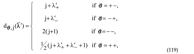
label them as indicated in Table 1 below,
with
and
specifying either the decay (+) or growth (-) of
the given JS at infinity, i.e., by definition
where
Table 1.
Classification of JS solutions on the infinite interval [1, ∞) based on their asymptotic behavior near the endpoints.
Table 1.
Classification of JS solutions on the infinite interval [1, ∞) based on their asymptotic behavior near the endpoints.
|
|
m |
|
+ + − |
|
|
− + − |
|
|
− − + |
|
|
− + + |
|
|
− + + |
|
|
+ − − |
|
|
− − − |
|
In following our olden study [43] on the Darboux transforms () of radial potentials, we use the letters and to specify the PFS near the singular endpoints 1
and ∞ (cases I and II in Quesne’s [72]
commonly used classification scheme of q-RSs according to their behavior near
the endpoints). We use the letters and [43] to identify
the eigenfunctions and respectively all the q-RSs (54)
not vanishing either at +1 or infinity (case III in Quesne’s classification
scheme). We underline the corresponding letter by tilde to indicate that the classification
of the JS solutions is done on the infinite interval (1, ∞). We mark the letter
by prime if the polynomial components of the given sequence of the q-RSs do not
include a constant. (Note that the ‘secondary’ sequences of such a type do not
exist for the potentials with infinitely many discrete energy levels which were
the focal point of Quesne’s analysis [72] .)
Note that the PFSs of the series
may exist only if the SLE does not have the
discrete energy spectrum. We thus need to consider the three sequences of the
quasi-rational PFSs: two
primary (starting from m=0) sequences
and
as well as the infinite secondary sequence
starting from
The primary sequence
is formed by classical Jacobi polynomials and
consequently may not have zeros between 1 and ∞. As expected, all the PFSs of
this type lie at the energies
below the lowest eigenvalue
The PFSs from the primary sequence
at the energies
do not have real zeros larger than 1 iff
Similarly the PFSs from the secondary sequence
at the energies

do not have real zeros larger than 1 iff
Before concluding this section, let us mention that
the change of variable (15) turns the quasi-rational functions (21) and (22)
into the eigenfunctions of the Schrödinger equation with the h-PT potential ,
as prescribed by (33) and (34) in [9] with and Note that the second parameter represents the
absolute value of the Jacobi index β
defined via (51) above. Also, the h-PT potential (31) in [9] depends on the squares of both Jacobi indexes
and therefore one only need to consider the positive values of α , keeping in mind that the potential is
repulsive only if α > 1/2.
Moreover, all the solutions of the Schrödinger equation with the h-PT potential
(31) in [9] are squarely normalizable if 1/2
< α < 1, i.e., the potential has
the discrete energy spectrum only for α
> 1, i.e., iff the ExpDiff lies within limit point (LP) range.
3. Use of RZTs for Constructing Xm-Jacobi DPSs
We say that the RZT is ‘rational’ (RRZT) if it uses
the quasi-rational TF
,
where
stands for the monomial product
with m simple zeros
, or, in other words, iff the TF has the rational
logarithmic derivative:
By definition of the RZT (see Appendix A for details), the quasi-rational
function
is the solution of the transformed CSLE
at the energy (25), with the density function defined via (7) for both intervals (-1,+1) and (1,∞). Each of the nodeless PFSs below the lowest eigenvalue can be used as the TF to generate the
of the CSLE (1).
Let us now take advantage of the fact that JRef CSL (1) is TFI [
73], namely, that quasi-rational function
is the solution of the JRef CSLE (1) with
replaced for |
, namely,
Let us also point to another remarkable feature of the JS q-RSs (23) – the Jacobi polynomials in the given sequence are multiplied by the same quasi-rational function and moreover the Jacobi indexes are independent of polynomial degrees [
1]. This is the direct consequence of the fact that this CSLE belongs to group A, which is also true for the corresponding Liouville potentials [
22].
Let us re-write both RCSLE (71) and
in the Riccati form:
and
respectively, where the symbolic expression
ld f[η] denotes the logarithmic derivative of the function f[η]. If the density function is identically equal to 1 then the derived expression turns into the standard supersymmetric representation of the quantum mechanical potential in terms of the superpotential represented by the logarithmic derivative of the TF
. In
Section 3 we will use a similar representation for the RefPFs of the
of the JRef CSLE (1) using the quasi-rational TFs (23).
Substituting the q-RS
into (75), coupled with (76), one finds
where [
1,
44]
It is worth mentioning that the derived expression (78) is valid on the both intervals (1,∞) and (-1,+1). It can be also trivially extended to two other CSLEs of group A with the Liouville potentials represented by the isotonic oscillator and by Morse potential (assuming that the Schrödinger equation in the latter case is converted to the Bessel-reference CSLE [
26].
Making use of (25) and (76) , coupled with
we can re-write (78) as
Taking into account that
and
along with
where
one can then directly verify that the derived expression turns into (27) in [
29] for m=1:
The quartet of the Liouville potentials for the RCSLE (71) defined in the four quadrant of the vector parameter
can be thus represented as follows:
with
For future references, we made the above expression to be applicable to the Liouville transformations on both intervals (1,∞) and (-1,+1), which constitutes the essence of the unified approach put forward in [
26] for m=1.
Taking into account that
and
One can verify that each of the potentials (87) vanishes at infinity, as expected.
Making use of the definition of the PF (79) for m=1:
along with (83)-(85) , we can re-write the Liouville potential for m=1 as
If we set
by analogy with (20), and take into account
we find that
for
and therefore
Substituting (98) into (94) for
then gives
The change of variable (15) on the interval (1,∞) then turns (99), with
, into the potential function (9) in [20}, while the change of variable η =
sin x converts (99), with
, into (3.5) in [
72], with A and B replaced in both cases for *A and *B respectively.
Let us draw reader’s attention to the fact that the two generally distinct branches of the potential (87) with
collapse into the same Bagchi-Quesne-Roychoudhury (BQR) potential for m=1, as expected from the rigorous analysis of the latter case in [
29]. The similar collapse takes place for the two other branches of this potential (
) but the resultant potential does not have discrete energy spectrum [
29] and therefore cannot be linked to any EOP sequence.
Coming back to the general case m ≥ 1, let us re-write the potential (87) for
as
While our expression (100) for the BQR potential (m=1) fully agrees with (15) in [
11], we detected some discrepancies between (100), with
, and the corresponding expression for this potential in [
11,
12].
First, both the potential (19) in [
11] and the following expression (37) for the rationally-extended
t-PT (Scarf I) potential (after being converted by the change of variable η =
sin x (|η|< 1) to its rational form (100) above) lack the term associated with the second derivative of the Jacobi polynomial in the right-hand side of (100). Since this derivative vanishes for the first-degree polynomial, one cannot detect the missed term simply by setting m=1 in the general formula. The mentioned term was also missed in (81) in [
12] or in the preceding expression (64) for the rationally-extended
t-PT (Scarf I) potential.
Disregarding the missed term, the rest of both cited expressions in [
12] match (100) for
, if we set
or, taking into account (97),
in agreement with the definition of these indexes in [
12]. It has been proven above that the potential (87) vanishes at infinity and therefore the function (81) in [
12] does not, keeping in mind that the omitted term tends to -m(m-1) as η→ ∞. (The reason for introducing the second pair of the potentials (82) and (83) following (81) in [
12] is unclear to me.)
As already pointed to in [
29], the parameter swap
does not result in the new potential. The potentials (19) in [
11] and (81) in [12} differ only by notation, with the constraint
reversed for
. This also true for he two potentials (12) and (15) listed in [
11] for m =1.
4. Pseudo-Wronskian Representation of Xm-Jacobi DPSs
Based on Rudyak and Zakhariev’s [
45] generic formula for the solutions of the transformed CSLE the general solution of the RCSLE
can be represented as
The gauge transformation
converts the RCSLE (103) into the algebraic Schrödinger equation
Substituting (106) into (104) then gives
where
Note that the latter function is holomorphic if the square-root of the density function in the JRef CSLE (1) is a PF. As a result, the RS function becomes the holomorphic ‘prepotential’ in Ho’s terms [
74,
75,
76,
77,
78]. In particular [
76], the Rosen-Morse [
79] potential represents the simplest case when
is the first-degree polynomial [
59]. The latter requirement also holds if the numerator of the PF
has a double zero [
80], with the Manning-Rosen [
81] potential (‘Eckart’ potential in I76[) as its limiting case).
The representation of the general solution of the algebraic Schrödinger equation in the form (109) provides the accurate mathematical basis for the conventional SUSY theory of rationally extended potentials utilized in [
12,
20,
30,
72]. It should be noticed in this connection that the renowned SUSY rules [CKS] for the changes in energy spectra due to DTs of the Schrödinger equation were originally formulated [38,39,82.83] for potentials with exponential tails at ±∞. The latter restriction forced the ODE under consideration to have the LP singularities at both quantization ends. The formulated rules were then extended by Sukumar [
84] to radial potentials without properly treating the LC range of the centrifugal barrier. Since then, the SUSY rules for the radial Schrödinger equation were duplicated without the proper examination of this non-trivial problem, with Gangopadhyaya et al.’s paper [
85] and Chapter 12 in [
86] as the only known-to-us exceptions.
If the ExpDiff for the pole at the origin lies within the LC range any solution is square integrable and the reg-RRZT with the TF of type does not results in the isospectral problem if the ExpDiff for the pole of the JRef CSLE (1) lies between 1 and 2. On the other hand, as discussed in more detail in subsection 5.3, we can still construct the corresponding EOP sequence using the polynomial components of the quasi-rational eigenfunctions of the prime SLE solved under the DBCs.
4.1.. of JS Solutions
Let us consider in parallel the four
of the q-RS
using the TFs
where
and
specify the quadrants of the vectors
and
respectively. By definition,
where
is equal to either + or - and
Let us prove that the corresponding solutions (104) of the RCSLE (103) at the common energy
have the quasi-rational form.
Theorem 1. RCSLE (103) has four infinite sequences of q-RSs, with the polynomial components represented by polynomial Wronskians for one of these sequences and by
of two Jacobi polynomials for three others.
Proof: In the simplest case
(
) the Wronskian of the two JS solutions takes form
where the polynomial of degree m+ j -1 in the right-hand side stands for the Wronskian of two Jacobi polynomials with the same pair of the indexes:
Taking into account that [53}
where
(see (91) in [
53] with
, and n replaced for j), we introduce the
polynomials via the relations:
and then re-write the Wronskian of the q-RSs (111) and (112),
as follows:
For
the latter expression turns into (116) with
Making use of (121) and (122), the RRZT of the q-RS (111),
can be thus represented in the following quasi-rational form:
which completes the proof of the Theorem 1. □
Representing the polynomials (120) in the alternative form
and
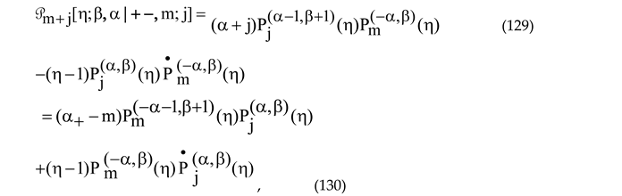
, we define the Xm-Jacobi DPSs of series J1 and J2 as follows
The two exceptional infinite polynomial sequences are interrelated by the interchange of the two indexes accompanied by the change in the argument, namely,
Despite the mentioned interdependence, we, in contrast with [
15,
16] prefer to treat these two X-OPSs separately and refer to them as being of series J1 and J2, in following the terminology suggested in [
3]. Note that, contrary to the definition (2.3) of these two series in [
3], with m=n,
and
in our notation, the indexes of the Jacobi polynomials in the right-hand side of (128) are independent of the polynomial degrees. It will be proven below that the polynomial sequences (127) satisfy the Bochner-type ODEs but violate the Bochner theorem since they do not start from a constant. We [
24] refer to them as the X
m-Jacobi DPSs of series J1 and J2, with no restrictions imposed on the Jacobi indexes other than their absolute values differ from 0 and 1.
In particular, setting
in (120) and (127) we come to (72) and (71) in [
16]:
and, consequently,
For m=1 the two X-DPSs collapse into the single X-DPS of series J [
29] which contains the X
1-Jacobi OPS [
31,
32] often referred to simply as ‘X
1-Jacobi orthogonal polynomials’. The term ‘X
1-Jacobi polynomials’ introduced by Yadav et al. [
23] (while referring to the X
1-Jacobi DPS of series J) seems satisfactory as far as one clearly understands that that that we deal here with a larger family of polynomials which contains both the X
1-Jacobi OPS and the only existent finite EOP sequence [
29].
On other hand, coming back to (101) and setting:
in (127) for
gives
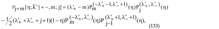
which brings us to the polynomial sequence (15) in [
10] (with ν standing j here). Note that (132) is consistent the m-independent definition of the indexes α and β in [
11]. With the latter correction, (15) in [
10] turns into (133) here, which is nothing but the X
m-Jacobi DPS of series J2 in our terms. It does contain both the X
m-Jacobi OPS [
15,
16] and the finite EOP sequences of type
used by Yadav et al. [
10,
11,
12,
13] to construct the analytical expression for the eigenfunctions of the rationally extended h-PT potential of the same type (and referred to in the cited papers simply as ‘X
m-Jacobi polynomials’.
Similarly, the ladders of lowering and raising operators introduced in [
14,[14,
89] act in the space spanned by the X
m-Jacobi DPS of series J2. The title ‘X
m-Jacobi orthogonal polynomials’ used for the subsection IV.A in [
14] seems misleading since the ladder relations analyzed by Yadav et al. are applicable for any values of the indexes α and β.
The polynomials belong to the X-OPS iff the indexes α and β are larger than -1 and have the same sign. The lowering operators necessarily bring these indexes into region where the polynomials do not belong to the X-OPS anymore. We postpone the thorough analysis of this issue for a separate publication.
Examination of the scattering amplitude (25) in [
10] reveals that it has poles on the imaginary positive
k-axis at
By choosing
and taking into account that, according to (97),
we confirm that the mentioned poles correspond to the bound energies (115), as expected. We thus assert the cited scattering amplitude was obtained in [
10] using the constraint 2B > 2A+1, but not the change of the notation suggested by the cited authors later in writing the potential function (19) in [
11].
Let us now consider the alternative quasi-rational representation of the Wronskian (122):

in terms of the so-called [
48] ‘polynomial determinant’ (PD)
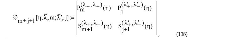
where

Originally [
8,
28] we used the PD decomposition as the universally applicable starting point for representing the
of JS solutions in the quasi-rational form for any admissible density function (see [
88] for an example). Yet the same year Gȯmez-Ullate et al. [
53] developed the powerful scheme allowing one to represent the
of JS solutions in the quasi-rational form, with the polynomial components represented by the
. The main advantage of using the
(instead of PDs) for the
of JS solutions discussed here is that the
, in contrast with PDs, remain finite at both singular points
and as a result form the X
m-Jacobi DPSs. Though we need to mention that this assertion does not generally retain for the polynomial components of the higher-order
in their
representation.
Comparing (137) with (122), one finds that
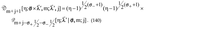
It directly follows from (140) that the PD and
representations become identical for
. Evaluating the polynomials (139) at
:
and substituting (141) into the right-hand side of (138) gives

We thus proved that the PD (138) remains finite at
, provided that this is true for the j-th degree Jacobi polynomial on the right. Out of the four PD sequences introduced by us in [
28] to generate the X
m-Jacobi DPSs, this was the only sequence which retains finite at ±1 and therefore spanned the DPS referred to by us for this reason as the X
m-Jacobi DPS of series D.
4.2. Bochner-Type ODEs for Four Xm-Jacobi DPSs
Let us draw reader’s attention to the fact that the magnitudes of the exponent parameters of the basic solution
in the right hand-side of (125):
represent the ExpDiffs for the poles of the RCSLE (15) at ±1 which implies that that each
polynomial remains finite at both poles at least if
are not negative integers with the absolute values smaller the polynomial degree. Substituting (41) into (29) and taking into account that the mentioned basis solution obeys the JRef CSLE (1) with
replaced for
we find that the
polynomial (38), with j standing for an arbitrary non-negative integer, satisfies the Bochner-type ODE:
where
is the abbreviated notation for the second-order differential operator
Keeping in mind that
we find that the coefficient function of the first derivative is represented by the fo;;owing polynomial of degree m+1:
and the ε-dependent polynomial of degree m representing the free term of the ODE (142) is linear in the energy:
Taking advantage of the definition of the second summand in (71) via (72), we assert that this term gives no contribution the polynomial (148), and therefore, bearing in mind that
and
we can represent the free-energy summand as
Setting
we can alternatively re-write (144) as the eigenvalue problem [
15,
16,
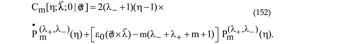
17]
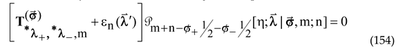
for the four exceptional differential operators
where
In particular, combining (153) with (133) for
:
one can then directly verify that the corresponding operator (155) precisely matches (2.2) in [
1][].
Let us remind the reader that the latter operator and the Liouville potential (100) were obtained using the same RefPF (82) as the starting point and that the Liouville potential is related to the RefPF via the elementary formula (88). This serves as the additional argument in support of the correctness of our expression for the Liouville potential of type
compared with the ones in [
11,
12].
It is worth stressing that any polynomial from the X
m-Jacobi DPS of series J2 is the eigen-polynomial of this operator with the eigenvalue
with n=m+j standing for the polynomial degree.
The X
m-Jacobi OPS of series J2 (and therefore its counter-part in the reflected argument) have been analyzed in a more rigorous way in [
15,
16,
17], and for this reason we focus solely on the finite EOP sequences. In
Section 5 we present the universal method for constructing the finite EOP sequences composed of
of the R-Jacobi polynomials. In the subsections 5.1, 5.2, and 5.3 we then focus on the EOPs forming the eigenfunctions of the rationally extended
h-PT potentials of types
,
, and
.
5. Isospectral Triplet of RCSLEs Solved via
of R-Jacobi Polynomials
Starting from this point, we discuss only the admissible RRZTs using the TFs
with no nodes in the interval (1,∞) for the specified ranges of the parameters
. In this Section we will consider only the TFs with the vector
lying in the first three quadrants. As demonstrated in [
1] using the Klein formula [
49], the admissible TFs also exist for certain segments of the vector
in the fourth quadrant, but this family of the finite EOP sequences lies beyond the scope of this paper.
To formulate the SLP on the interval (1,∞) we (by analogy with the analysis) presented in subsection 2.3 for the JRef CSLE) first convert the RCSLE (103) to its prime form
and then solve it under the DBCs:
The zero-energy free term in the SLE (159) is related to the RefPF of the RCSLE via the same elementary formula:
Taking into account that
we confirm that the ChExps of the Frobenius solutions for the pole at +1 have the same absolute value, while differing by their sign. The ExpDiff for the pole of the RCSLE (103) at infinity turned out to be energy-dependent. We have already proved that the second-order poles in the second and third summands nullify each other, and therefore
We thus assert that the ChExps of the Frobenius solutions for the pole at ∞ are real only at negative energies and have in this case the same non-zero absolute valuewhile differing by their sign.
Combining (163) with the similar limit
for the pole at +1, we conclude that the PFSs of the
p-SLE (159) near both singular endpoints are unambiguously determined by the DBCs.
By applying the RRZT with the admissible TF
to the eigenfunction
and then converting the resultant transform (125) to its prime form:
where
Suppose that the q-RSs (166) obey the DBCs
for any j ≤ j
max and therefore represent as the eigensolutions of the Sturm–Liouville problem solved under the DBCs. (We will analyze this assertion on the case-by-case basis in subsections 2.1, 2.2, and 2.3 below for the vector
lying in the first, second and third quadrant accordingly.) It has been proven in [
56] that the eigenfunction of the generic SLE solved under the DBCs must be mutually orthogonal with the weight (31) on the infinite interval in question:
Consequently, the polynomial components of the quasi-rational eigenfunctions (165) must be mutually orthogonal with the m-dependent weight
namely,
Let us now demonstrate the power of the developed formalism by proving that the q-RSs (165) form the complete set of the eigenfunctions for the formulated Dirichlet problem.
Theorem 2: The Dirichlet problem for the p-SLE (159) defined on the infinite positive interval [1,∞) does not have any solutions other than the eigenfunctions (176), assuming that the pole of the corresponding CSLE (103) at +1 is LP.
Proof: Suppose that the given Dirichlet problem has a solution
at an energy for 0 ≤ j ≤ jmax.
The RRZT of the RCSLE (103) with the TF
converts the extraneous eigenfunction into the following q-RS of the
p-SLE (29):

Let now remind the reader that the extraneous eigenfunction (like any other) must decay as
in the limit
. Examination of the sum:
then shows that it vanishes at the lower end of the interval (1, ∞) as far as the pole the
RCSLE (103) at +1 lies in the LP region ().
Furthermore, one can easily verify that the solution in question also vanishes in the limit η → ∞ and therefore represents an eigenfunction of the p-SLE (36) with an eigenvalue differing from any of the eigenvalues (40). This result contradicts to the fact that the cited energies represent the complete discrete energy spectrum of the given Dirichlet problem. We thus confirmed that the p-SLE (159) solved under the DBCs (160) may not have eigenvalues other than (40) in the LP range of the parameter . □
5.1. Infinitely Many EOP Sequences of Series
Let us start from the vector
lying in the first quadrant:
Consequently, the seed polynomial in the denominator of the weight (169) turns into the classical Jacobi polynomial with positive indexes and therefore all the poles of the RCSLE (103) are located in the closed interval [-1,+1]. Ironically, this most obvious case has never been discussed in the literature and our study of these EOP sequences in [
24] was left without a proper response.
The finite polynomial sequence under consideration belongs to the X
m-Jacobi DPS of series J1 specified by the upper sign in (127). Taking into account (166), we can represent this polynomial subset as
Setting z = −
,
, we come to the polynomials (72) in [
16]:
with the interchanged degrees m and j, i.e.,
We thus proved that the polynomial (172) converted to its monic form coincides with the monic m-th degree polynomial from the X
j-Jacobi OPS of series J1 [
24]. This implies that the polynomials (174) arranged into the infinite row (m=1,2,..,) at fixed j are mutually orthogonal with the weight
(see (87) in [
16]). We thus come to the (j
max+1)
∞ rectilinear polynomial matrix mentioned in Introduction.
With the given choice of the quadrant for the vector
and
, the q-RSs (165) take the form:
making the DBC at η=1 trivially hold. (As expected, the absolute values of the power exponents
of η
coincide with halves of the ExpDiffs
for the poles of the RCSLE (103) at
1, as far as the pole at -1 is LP.) Taking into account that
we assert that
which confirms that the q-RS (175) is the eigenfunction of the
p-SLE (159) and therefore its polynomial components are mutually orthogonal with the weight
Since the RCSLE (103)
is analytically solvable only for
, Theorem 2 assures the exact solvability of the Dirichlet problem in question. From the perspective of the quantum mechanical applications, the corresponding Liouville potential (100) with 1 <
< 2 represents the very specific case because its SUSY partner,
h-PT potential with the positive parameter
smaller than 1 or
has only the CDBESs. Within the specified range of the potential parameters, there is no way how our results can be reproduced using the conventional rules of the SUSY quantum mechanics.
5.2. Infinitely Many EOP Sequences of Series
Let us now consider the peculiar case when both vector
and
lie in the same (second) quadrant (
). The admissible TFs of this type exist only for finite EOP sequences. According to the inequality (65), the q-RS
is admissible for any
from the infinite sequence of the positive integers starting from
. Substituting (116) into (124) with
=
gives
As expected, the absolute values of the power exponents of η coincide with halves of the ExpDiffs for the poles of the RCSLE (103) at. Since and therefore , the q-RS (182) necessarily vanishes at +1.
To confirm the DBCs (167) at the upper end of the quantization interval, first note that the PF in the right-hand side of (182) grows at large η as ηj-1. Taking into account that the q-RSs and have the same asymptotics at infinity while the eigenfunction vanishes at this endpoint, we conclude that this should be the more so true for the q-RS (182).
Since
, Theorem 2 again assures the exact solvability of the Dirichlet problem in question. Once more, the corresponding Liouville potential (100) with 1 <
< 2 and
is not covered by the conventional rules of the SUSY quantum mechanics. In Grandati’s notation [
9]:
so his analysis is applicable solely to the parameter range
On the contrary, the technique developed here made it possible to extend the discussion of the rationally-extended
h-PT potentials to the parameter range
The border case
requires a more cautious analysis.
I doubt that the extension of the domain definition for the parameter α to negative values (α > -
in (31) in [
9]) makes any sense in the quantum-mechanical studies of the
h-PT potential and its rational extensions. Though it is possible that formulating the appropriate PSLPs would allow one to construct finite EOP sequences of types
and
for -1< α < 0 the q-RSs composed of these polynomials could be hardly applied in physics.
5.3. Finitely Many EOP Sequences of Series
By placing the vector
into the third quadrant, we finally come to the case which so far has attracted much more attention from the physicists [
10,
11,
12,
13] – the rationally extended
h-PT potential of type
constructed using the finite number of the nodeless TFs
under the constraint (63). In the sharp contrast with the two cases discussed above, the RRZTs in question decreases by 1 the ExpDiff for the pole at +1. As a result, the
p-SLE (159) can be analytically solved within the LC range of the ExpDiff
. However, we were unable to prove that the SLP is exactly solvable in this case.
With
,
and
the q-RSs (165) take the form:
As expected, the absolute values of the power exponents of η coincide with halves of the ExpDiffs for the poles of the RCSLE (103) at 1, as far as the pole at +1 is LP. Though the q-RSs automatically vanish at +1, it should be noticed that we excluded out of consideration the LC region for the pole of the JRef CSLE (1) at +1, when . Since is the eigenfunction of the p-SLE (29) solved under the DBCs (35), the q-RS (183) must also vanish at infinity and therefore represents the eigenfunction of the SLP under discussion.
Note that, compared with the two other SLPs discussed above, the
p-SLE (159) with
is analytically solvable in the LC region for its pole at +1. While Theorem 2 does not guarantee the exact solvability of this SLP in this case, we can point to another remarkable development by Yadav et al. [
10]. Namely, they calculated the scattering amplitude for the rationally extended
h-PT potential of the given type and the inspection of the derived expression (25) in [
10] reveals that it has exactly the same poles on the imaginary positive
k-axis as the scattering amplitude for the
h-PT potential. This confirms that the DT in question does not create new bound energy states, in agreement with Theorem 2. It should be however stressed that the expression for the scattering amplitude (25) in [
10] makes no distinction between the LP and LC singularities. It seems interesting to re-examine the derivation of the cited expression to make sure that the specifics of the LC region was correctly accounted for but we postpone this analysis for future studies.
It is also interesting to mention the basic PFS of the given type (
=0) have been used in [
85] to study the DTs between the LP and LC regions of the h-PT potential. Keeping in mind that
in our terms, we find the close connection between the analysis presented in [
85] and the current discussion. Namely, the cited authors pick up the
of each eigenfunction (well-defined in the LP region) as the special representative of the CDBESs for the eigenvalue. As more recently proven in [
48], the
of the eigenfunction of the p-SLE with the LP singularities at the ends necessarily obeys the DBCs under consideration. In other words, Gangopadhyaya et al select the bound energy states described by the PFSs at the origin, with a clear resemblance to our prescriptions.
6. Discussion
The paper is based on the three core notions advanced by the author in the aforementioned publications. One of them is the scrupulous analysis of the RCSLEs obtained by the RRZTs of the JRef CSLE (1). As pointed to in Introduction, any RRZT of the RCSLE is directly related to a DT of the corresponding Liouville potential and as a result this part of our studies lays the rigorous foundation for the SUSY theory of the quantum-mechanical potentials solvable by polynomials.
Another important element of our approach is the concept of the ‘prime’ SLE chosen in such a way that the two ChExps for the poles at the endpoints differ only by sign. As a result, the energy spectrum of the given Sturm-Liouville problem can be obtained by solving the prime SLE under the DBCs. This in turn allows one to take advantage of the rigorous theorems proven in [
56] for eigenfunctions of the generic SLE solved under the DBCs.
Finally, we put forward the concept of the X-Jacobi DPSs formed by polynomial solutions of the Bochner-type ODEs. Since the X-DPSs either do not start from a constant or lack a first-degree polynomial, they do not satisfy the Bochner theorem [
36], as originally noticed by Gȯmez-Ullate et al. [
33] in the context of the discovered by them X
1-Jacobi OPS. In general, each X-Jacobi OPS belongs to one of the X-Jacobi DPSs. If the given X-Jacobi DPS does contain a X-Jacobi OPS, then we say that they belong to the same series. This is why we [
8] started referring to the X
m-Jacobi DPS of series D [
24] as being of series J3, after becoming aware of Grandati and Bérard’s [
50] discovery of the X
m-Jacobi OPS of series J3 for even m. (We still continue to refer the X
m-Jacobi DPS of series D as being of series J3 for odd m even though the latter do not contain any OPSs.) (As proven in [
28], the X
1-Jacobi DPS of series D does not contain any finite EOP sequences either.)
In addition to the two finite EOP sequences identified in [
9] and in [
10,
11] accordingly, our original research [
24] discovered the (undeniably new to our knowledge) finite EOP sequences of type
, which were constructed using the q-RTFs composed of the classical Jacobi polynomials. Since all the zeros of the latter polynomials lie between -1 and +1, the q-RTFs of this kind (representing the PFSs at the origin) do not have nodes within the quantization interval (+1,∞). The very remarkable feature of the finite EOP sequences constructed in such a way [
24] is that they can be arranged into the rectilinear polynomial matrix with a finite number of rows and an infinite number of columns representing the X-Jacobi OPSs of series J1 and
of the R-Jacobi polynomials accordingly.
Compared with the cited preprints [
1,
8,
24], the brand new element of the current analysis, is the proof that the X
m-Jacobi DPSs of series J1 and J2 are composed of the
of two Jacobi polynomials [
51] , and therefore this is also true for their infinite and finite X-orthogonal subsets. In particular the mentioned rectilinear polynomial matrix is formed by the
of the classical Jacobi and R-Jacobi polynomials, respectively.
This result for the X
m-Jacobi DPS of series J1 has a very interesting far-reaching implications, making it possible to obtain analytical expressions for both infinite and finite EOP sequences using the PFSs of the same type
as seed functions. In [
59] we have discussed the RCSLEs obtained from the JRef CSLE (1) using the seed Jacobi polynomials with the same indexes. Since the RDCTs using the seed functions of types
and
are specified by same series of the Maya diagrams, any RCSLE using an arbitrary combination of these seed functions can be alternatively obtained by considering only infinitely many combinations
of the PFSs of types
[
51,
73]. In particular, the Liouville potentials of type
discussed above can be alternatively obtained by means of the
th-order RDCT with the seed functions
[
22,
73].
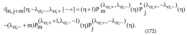
One can easily verify that the quasi-rational functions defined via the relations
where
, constitute polynomials of degree
, where
The explicit expression for the ‘simple’
polynomials (184) can be easily obtained using (92) in [
51] and will be examined in a separate paper. As expected, the ‘simple’
polynomials (184) turn into the Xm-Jacobi DPSs of series J1 for p=1.
It has been proven in [
25] that the ExpDiffs for the poles of the RCSLE
at
are given by the simple formula
The corresponding eigenfunctions has the form [
90]:
where
Representing (189) as
we find that the absolute values of the power exponents of η
coincide with halves of the ExpDiffs (187) and therefore the simple
polynomials (184) form a X-Jacobi DPS, which will be referred to by us as being of series
. A similar X-Jacobi DPS of series
simply constitutes another representation of one of the X-DPSs mentioned above and might be dropped though it would come with a catch: the corresponding net of the X-Jacobi OPSs (
,
) starts from the infinite manifold of the X
m-Jacobi OPSs in the conventional sense [
15,
16,
17].
If we choose and restrict j from above by the constraint j ≤ jmax, then the resultantof the R-Jacobi polynomials form the finite EOP sequences of series. We thus come to the very broad brand families of both infinite and finite EOP sequences, which will be examined in detail in a separate publication.
One can also combine the nodeless PFSs of type
with the juxtaposed pairs of the eigenfunctions (type
) to construct the RCSLEs quantized by the finite EOP sequences composed of the Wronskian transforms of the R-Jacobi polynomials, similar to the finite EOP sequences formed by the Wronskian transforms of the R-Bessel and R-Jacobi polynomials [
26,
28].
The general case using the seed functions of all the four types,,,, and represent a much more challenging problem.