Submitted:
16 February 2025
Posted:
17 February 2025
You are already at the latest version
Abstract
This study analyses the relationship between liquidity and debt management ratios and their impact on the financial performance of South Asian airlines from 2011 to 2022. The application of GARCH and TARCH models reveals a nuanced relationship among these factors. Open money, evidenced by strong positive lagged relationships with liquidity ratios and Return on Equity (ROE), plays a crucial role in financial prosperity. Conversely, elevated debt levels, indicated by negative lagged correlations with ROE, exert a detrimental effect. A long-term equilibrium relationship between the factors highlights their interconnectedness and the stability of this dynamic. However, potential limitations such as heteroscedasticity and neglected factors indicate the need for further investigation. This study emphasises the significance of effective liquidity management and prudent debt strategies for South Asian airlines to enhance financial performance and ensure long-term sustainability. Future research may explore the differential effects among various airline types and the influence of external factors, thereby facilitating enhanced financial practices and a robust aviation sector in the region.
Keywords:
accounting
; finance
; retrun on assets
; current ratio
; debt ratio
1. Introduction
When it comes to the performance of the organizations, competition, expansion, the name of the organization, and their financial data are always crucial. An effective accounting information system enables the generation, maintenance, and formulation of essential and accurate reports. Both small and large businesses necessitate precise accounting records to assess their progress. An effective accounting and finance department is crucial for overall business growth and the success of individual enterprises. The capital structure of a company consists of debt and long-term capital. A business utilises it to acquire essential assets or to address a capital shortfall. The investor possesses a claim on a company's assets pertaining to both debt and equity. Correct employment of these is essential. Employ these resources to finance productive assets, enabling the business to generate sufficient revenue (Aman & Altass, 2023).
Businesses aim to evaluate and measure profitable successes to enhance their understanding of organisational prospects, developments, and advancements. A business succeeds by achieving its goals and adhering to its standards. A management system that meets funder obligations while fulfilling company objectives is enhanced by the assessment of financial performance. This review aims to enhance economic performance by utilising Return on Assets (ROA) to improve its value and upgrade the company's financial performance. The assessment of Return on Assets indicates that the investment in profitable assets is contingent upon the viability of capital (Hermuningsih et al., 2023).
The liquidity of a company indicates its ability to fulfil immediate obligations. Financial ratios, such as the current, cash, and quick ratios, are employed to assess it. A company with sufficient liquidity can employ its current assets, including cash, inventories, and receivables, to meet its short-term obligations. Also, the corporation can utilize the liquidity to jump all over immediately or make the most of possible chances that might boost profitability (Bhattacharya, 2023; Tang et al., 2024).
Liquidity refers to the ability of a company to fulfil its short-term obligations, and its significance becomes evident when assessing the consequences of a company's inability to do so. A company's failure to pay its creditors can be attributed to various factors. The company possesses no assets whatsoever. Second, although the company possesses cash, its ability to cover current liabilities is inadequate. A lack of liquidity could force the company to liquidate its fixed assets and investments or, in the worst case, result in bankruptcy (Sany & Yonatan, 2023).
This study will evaluate each ratio to determine the extent of the relationship between the current, quick, cash, debt, and debt-to-equity ratios and Return on Equity.
The purpose of this study is to provide solutions to the following problems that have been posed: To recognize
Whether the current ratio significantly affects the Return on equity of Airline companies in South Asian economies.
Whether the Quick ratio has a significant effect on the Return on equity of airline companies in South Asian economies
Whether the cash ratio has a significant effect on the Return on equity of airline companies in South Asian economies.
Whether the Debt ratio significantly affects the companies' Return on equity in South Asian economies.
Whether the Debt-to-equity ratio significantly affects the Return on equity of Airline companies in South Asian economies.
2. Literature Review
2.1. Liquidity and Financail Perfromance
Contemporary financial theory posits that the airline firm seeks to maximise value for its shareholders. Furthermore, it is considered the primary financial objective of the company. Financial management seeks to inform decisions that enable a firm to attain business excellence, especially in value creation (Hiadlovsk et al., 2016). Liquidity is an essential tool for every organisation. The organisation can achieve this by transforming liabilities into assets. Liquidity reflects a corporation's capacity to settle its debts, whether in the short term or long term. Liquidity influences performance, as a financially sound company generally exhibits strong performance and maintains adequate liquidity. The company's operational confidence influences its liquidity (Waswa et al., 2018; Raza et al., 2024; Raza et al., 2023; Mugambi et al., 2023).
Nanda and Panda (2018) assert that a low level of liquidity within an organisation may diminish its procurement capacity due to increased credit requirements, subsequently impacting profitability negatively. The organization's productivity could experience the ill effects of low liquidity levels. A company facing insufficient funds to meet its obligations may resort to external borrowing, which incurs interest and subsequently reduces its profit margins. The company must liquidate investments and non-current assets to settle its debt if it depletes its cash reserves prior to the due date of its obligations.
Previous studies (Hiadlovsk et al., 2016; Xiang et al., 2022; Khan et al., 2022) emphasise the significance of effective liquidity management in relation to a company's financial performance. Confusion persists regarding the relationship between liquidity and profit. Popular belief suggests that a less liquid asset may yield a higher expected return, indicating a positive relationship between expected returns and liquidity (Amihud & Levi, 2023).
Kaodui et al. (2020) examined the influence of liquidity on the financial performance of firms listed on the Ghana Stock Exchange. The findings of the study indicate that liquidity positively and significantly influences the financial performance of companies listed on the Ghana Stock Exchange. Additionally, causal relationships existed between company liquidity and financial performance on the Ghana Stock Exchange. Chasha, Kavele, and Guandaru (2022) concluded that working capital management and liquidity have a statistically significant effect on the financial performance of small and medium-sized enterprises in Kenya. A study on the impact of liquidity on the financial performance of Kenyan insurance enterprises was conducted by Kariuki, Muturi, and Njeru (2021). It was found that liquidity significantly and positively influenced financial performance. Since the study used panel data, reporting on diagnostic tests was suitable to reduce the possibility of drawing erroneous findings (Tang et al., 2024). Furthermore, because star-rated hotels and insurance businesses are exposed to separate industry-specific hazards, none of the study's conclusions can be applied to their respective industries, creating population gaps. Based on the above literature, the primary goal of this research is to clarify the significant relationship between liquidity and financial performance of the Airline companies in South Asia.
2.2. Debt Management and Financial Perfromance
Ratio analysis involves the connection of various estimations derived from financial statements through the use of financial ratios. This financial ratio analysis reveals important correlations between reported estimates and can be utilised to evaluate the company's financial performance and condition. The current ratio is a financial metric that assesses a company's liquidity by dividing its current assets by its current liabilities. This demonstrates to investigators and investors how a company may leverage its assets to address debt and obligations (Ciptawan & Frandijaja, 2022). The current ratio indicates the extent to which a company's current assets can cover its short-term liabilities, thereby evaluating the corporation's ability to meet its short-term obligations. An increase in the current ratio indicates a decrease in the amount of current assets available to meet current obligations, and conversely, a decrease in the current ratio suggests an increase in available current assets. The anticipated profit will depend on the total resources invested. This illustrates the impact of the current ratio on return on assets (Irman & Purwati, 2020).
The quick ratio, or acid test ratio, evaluates a company's ability to fulfil its short-term financial obligations using its most liquid assets. Liquidity ratios assess a business's capacity to meet its short-term obligations. This study utilises a rapid ratio that omits inventory from its calculation as an indicator of liquidity. Due to the prolonged duration required to convert inventory into cash and the associated low confidence level, it is feasible that the inventory account may be excluded from the computation. As the quick ratio increases, investors are likely to experience higher stock returns. Previous studies by Tarmizi (2018) and Wijaya and Sedana (2020) indicate that the quick ratio has a significant impact on returns on equity. Hartina (2021) indicated that the current ratio, a measure of liquidity, exerts an influence. The increase in the current ratio correlates with an enhancement in profitability, as indicated by the Return on Assets, demonstrating a positive relationship with profitability.
The debt-to-equity ratio quantifies the relationship between debt and equity. The debt-to-equity ratio is calculated by dividing total debt by total equity (Raza et al., 2022). The debt-to-equity ratio quantifies the relationship between funds sourced from creditors and those provided by business owners. The determination of the capital amount of each rupiah utilised as debt collateral is based on the debt-to-equity ratio. The owner's capital available for loan collateral diminishes with an increase in the debt-to-equity ratio. Focussing on debt-to-equity is essential for shaping the company's dividend policy. The debt-to-equity ratio indicates the amount of debt a company owes (Shabrina & Hadian, 2021; Raza et al., 2023). The debt-to-equity ratio (DER) is a solvency metric that assesses a company's total debt relative to its equity. Investors frequently employ this ratio to assess the company's debt in relation to its equity ownership. Analysts and investors regularly employ the debt-to-equity ratio to assess the level of debt a firm holds in relation to its shareholders' equity. The corporation will employ its assets to settle its debt in the event that its equity is insufficient. The utilisation of assets will affect the return on assets financed by debt, as the achieved return percentage should be substantial; however, the level of asset investment is insufficient. This concept illustrates the impact of the debt-to-equity ratio on return on assets (Hasanudin, 2023).
Companies primarily utilise debt to raise capital and enhance potential earnings for shareholders; however, neglecting the appropriate level of debt or leverage can adversely affect the company's profitability. This aligns with the findings of Putra and Badjra (2015), which indicate that leverage has a significant negative impact on profitability. Hartinaa's (2021) study asserts that debt has a significant positive effect on profitability and return on equity. Financial performance is evaluated through the firm's financial recording activities to determine the extent of the company's achievement against predetermined standards.
H1= the current ratio has a significant impact on the return on equity of airline companies in South Asian economies.
H2= the quick ratio has a significant impact on the return on equity of airline companies in South Asian economies.
H3= the cash ratio has a significant impact on the return on equity of airline companies in South Asian economies.
H4= the debt to assets ratio has a significant impact on the return on equity of airline companies in South Asian economies.
H5= the debt to equity ratio significantly influences the Return on Equity of airline companies in South Asian economies.
3. Methodology
The study analyzed data from fifteen South Asian airlines operating from 2011 to 2022. The annual reports of the firms, specifically their balance sheets, income statements, cash flow statements, and equity statements, were meticulously analyzed to extract financial data (Alamgir, 2023; Iqbal, 2021). The independent variables in this research are liquidity ratios, specifically the current ratio, quick ratio, and cash ratio, as well as debt management ratios, including the debt ratio and debt-to-equity ratio. This study designates ROE as the dependent variable.

Table 1.
Data description.
| Variable | Abbreviations | Basic Formulas | Source |
|---|---|---|---|
| Current ratio | CR | Current Assets / Current Liabilities | Companies Financial Statement |
| Quick ratio | Q.R. | (Current Assets - Inventory) / Current Liabilities | Companies Financial Statement |
| Cash ratio | CaR | Cash and cash equivalents / Current liabilities | Companies Financial Statement |
| Debt ratio | D.R. | Total Debt / Total Assets | Companies Financial Statement |
| Debt to equity ratio | DER | Total Debt / Total Equity | Companies Financial Statement |
| Return on equity | ROE | Net Profit / Shareholders' Equity | Companies Financial Statement |
The following equations will be used to model the relationships between the variables:
where ROE is the Return on equity; C.R. is the current ratio; Q.R. is the quick ratio; C.R. cash ratio; D.R. is the debt ratio; DER is the debt-to-equity ratio; β0 is the intercept; β1, β2, β3, β4, and β5 are the coefficients; ε is the Error term.
ROE = β0 + β1CR + β2QR + β3CaR + β4DR + β5DER + ε
Descriptive statistics were employed to assess the variability, central tendency, and range of the teach variable (Shannon, 2011). This analysis included standard deviations, minimum and maximum values, and averages. A standard deviation is generally expected to be less than twice the mean; however, typical values for standard deviations may vary depending on the type of data being analysed. Hair et al. employed Pearson lagged coefficients to examine the strength and influence of each independent variable's direct relationship with the dependent variable. Hair and colleagues (2021).
A total negative lag is indicated by a value of -1, no relationship is represented by a value of 0, and a perfect positive lag is indicated by a value of 1. Pearson lagged coefficients typically fall within these ranges. Calculations for Difference Stationary Processes Enhanced The Augmented Dickey-Fuller (ADF) tests were conducted to verify stationarity and eliminate time-series dependency in the variables (Dickey & Fuller, 1979). The ADF test often yields results that do not precisely equal -2.96. Calculations pertaining to cointegration. Johansen cointegration tests were employed to assess the existence of a long-term equilibrium relationship among the variables. Hassani (2023). Assessments of Cointegration: Johansen cointegration tests were used to decide whether a long-run equilibrium relationship between the variables existed. Hassani (2023). The Johansen cointegration test typically has a p-value of less than 0.05. Ordinary Least Squares regression was employed to determine the direct relationship between the independent variables and Return on Equity (ROE). Siddiqui (2021) For the R-squared, a worth of 0.7 or above is respected as typical, and for the F-measurement, a p-worth of under 0.05 is viewed as ordinary. The evaluation of heteroscedasticity using the Breusch-Pagan and Weiß tests: Heteroscedasticity is distinguished involving tests for heteroscedasticity when the OLS supposition that the variance of the residuals is steady for all observations is broken Siddiqui, (2021) The Breusch-Pagan test is thought to have a usual p-value of more than 0.05. The residuals were examined for autolagged and serial lagged using Durbin-Watson broken Siddiqui (2021). The typical range of results for the Durbin-Watson test is 1.5 to 2.5. Q-statistics for Ljung-Box autolagged estimations: Ljung-Box Q-statistics were used to investigate further autolagged up to a predefined lag order (Box & Pierce, 1970). The Ljung-Box Q-statistic is typical when the p-value is greater than 0.05. Ramsey RESET tests were conducted to check for omitted variable bias, suggesting the existence of pertinent variables that were left out of the model (Ramsey, 1969). A normal outcome for the Ramsey RESET test is indicated by a p-value greater than 0.05.
Recursive coefficient estimates were used to examine the regression model's long-term stability (Belsley et al., 1980). The normal values of recursive coefficients must hold throughout time. To account for both the conditional heteroscedasticity in the residuals and the permanent asymmetric effects, estimates of the PARCH model (Permanent Asymmetric Component of Heteroscedasticity in Regression) were performed (Engle, 1982). Normal values for PARCH model parameters may vary depending on the kind of data being examined, but in general, the model should account for a substantial portion of the residual variability, and the coefficients should be statistically significant. GARCH (Generalised Autoregressive Conditional Heteroscedasticity) and TARCH (Threshold Autoregressive Conditional Heteroscedasticity) estimations were performed to mimic the dynamic nature of volatility in the residuals (Engle, 1982; MA, 2020). The normal values for the GARCH and TARCH model parameters can also vary depending on the kind of data being examined, but in general, the models should capture the dynamic nature of volatility in the residuals, and the coefficients should be statistically significant. The econometric analysis was carried out using EViews 12 software.
4. Empirical Results and Discussions
This research aims to explore how liquidity and debt ratios effects financial performance of south Asian airline industry.
Table 2 shows the mean current ratio of the sample is 0.63, indicating that for each dollar of current liabilities, businesses possess 0.63 in current assets. The standard deviation of 0.49 indicates a modest variation in current ratios among the enterprises. A distribution with a skewness of 0.96 suggests a rightward skew, indicating that while the majority of organisations exhibit ratios near the mean, a minority possess significantly lower ratios. The kurtosis of 3.99 indicates a distribution that is somewhat platykurtic, exhibiting a flatter profile compared to a normal distribution. A standard deviation of 6.25 signifies considerable variability in the quick ratios across the firms. Numerous organisations exhibit low quick ratios, whereas others approach the mean, as evidenced by a skewness of 5.72, indicating a significantly right-skewed distribution. The distribution exhibits significant leptokurtosis, characterised by a taller and thinner profile compared to a normal distribution, as evidenced by a kurtosis value of 35.76. The sample's mean cash ratio indicates that companies possessed $9.96 in cash for each dollar of current obligations. The standard deviation of 43.09 signifies considerable variability in the cash ratios across the organisations. A right-skewed distribution is indicated by a skewness of 4.51, suggesting that while the majority of organisations exhibit ratios near the mean, a minority display significantly lower ratios. A leptokurtic distribution, characterised by a greater peak and thinner tails compared to a normal distribution, is indicated by a kurtosis value of 21.83. The mean debt ratio of the sample is 94.48%, signifying that businesses possess $94.48 in debt for every $100 in total assets. The standard deviation of 123.26% signifies considerable variability in the debt ratios of the enterprises.
The right-skewed distribution, with a skewness of 1.72, suggests that while most firms have debt ratios near the mean, a significant number exhibit very high debt ratios. The kurtosis of 5.09 indicates a platykurtic distribution, as the distribution is flatter than that of a normal distribution. The mean debt-to-equity ratio of the sample is 55.71%, indicating that for every $100 in equity, businesses carry $55.71 in debt. Return on equity (ROE) serves as an indicator of a business's success, reflecting the profit generated by the firm for each dollar of shareholder equity. The average ROE of 14.16% indicates that the sample firms profit from their equity investment. A better yield on equity ROE is ideal since it shows that a business is making beneficial use of its resources.
Table 3 shows that the quick ratio and current ratio exhibit a perfect positive correlation. A favourable correlation exists between the money ratio and the current ratio. A weak positive correlation exists between the debt-to-current ratios. The weak inverse correlation between the debt-to-equity ratio and the current ratio Notable relationship between return on equity and current ratio there is a notable relationship between the debt ratio and the debt-to-equity ratio. A weak negative correlation exists between the debt ratio and return on equity. The relationship between the ratio of debt to equity and return on equity exhibits a significantly negative lagged effect. Lagged calculations indicate the presence of multiple delays among the various indicators of liquidity, debt, and profitability. These connections may result from various elements, including the business's industry, development plan, and finance choices. Airline companies exhibiting higher debt levels typically demonstrate lower returns on equity, attributable to the significant inverse relationship between the debt-to-equity ratio and returns on equity. Businesses with higher debt levels often incur elevated interest costs, which may adversely affect their profitability. Comprehending the financial performance of airline companies necessitates an analysis that extends beyond mere recognition of the interconnections among financial metrics. Additional influences may include the regulatory environment of the company, the competitive landscape, and the overall economic conditions
Analysts employ the Distinction Fixed Interaction test to assess whether a period series variable exhibits a Distinction Fixed Cycle. A non-fixed variable is characterised by mean fluctuations that do not remain consistent over time and exhibit a distinction of fixed interaction. In this context, interpreting the outcomes of statistical tests that rely on stationarity can be difficult. The fixed cycle test was employed to determine whether the time series variables were stationary prior to conducting a regression analysis focused on the effects of liquidity and debt on the managerial ratios influencing the financial performance of airline companies. Prior to its application in a relapse examination, a variable characterised by a fixed cycle must be differentiated or modified by calculating the difference between two successive values. The table 4 presents the findings from the Phillips-Perron (P.P) and Augmented Dickey-Fuller (ADF) tests regarding the Return on Equity, current ratio, quick ratio, cash ratio, and debt ratios. The results indicate that each variable is stationary in its initial differences. The variables do not necessitate differencing when employing regression analysis. Difference Stationary Process tests are essential for preventing misleading regression. When two non-stationary time series variables are correlated, a statistical phenomenon referred to as spurious regression may occur. The presence of lag does not necessarily indicate a causal relationship between the two variables. The outcome may result from both factors moving in a similar direction. The verification of the study's conclusions was facilitated, rendering them reliable and suitable for consideration by legislators and airline corporations in decision-making processes.
Table 5 shows the cointegration analysis indicates a long-term equilibrium relationship between financial performance metrics for airline companies and liquidity and debt management ratios. This suggests a stable relationship between these variables over time, rather than random co-movement. This result significantly influences the understanding of the dynamic interaction between financial strategies and airline performance.
The relationship between liquidity and debt management ratios—such as the current ratio, quick ratio, cash ratio, debt ratio, and debt-to-equity ratio—and financial performance, specifically return on equity (ROE) for aircraft companies, is revealed by the OLS estimates presented in Table 6. The table presents the coefficients, standard errors, t-statistics, and p-values for each independent variable in the regression model. The Current ratio exhibits a positive correlation with ROE; however, it lacks statistical significance. Although a negative relationship exists between the Quick ratio and ROE, it is not statistically significant. A positive and statistically significant relationship is observed between the cash ratio and return on equity (ROE). It indicates that airlines with greater cash reserves may invest in growth opportunities with substantial assets, thereby enhancing their financial performance. The relationship between the debt ratio and ROE is negative; however, it lacks statistical significance. Although a positive relationship exists between the debt-to-equity ratio and ROE, it is not statistically significant. Return to equity: Even though there is a positive connection between ROE and Return on equity, it is not statistically critical.
The model demonstrates an R-squared value of 0.3372, indicating it accounts for approximately 34% of the variance in ROE among carrier organisations. The adjusted R-squared value of 0.2500 is lower, given the number of independent variables in the model. The model demonstrates a strong fit to the data. It is plausible that additional variables not accounted for in the model affect ROE. Two statistical measures employed to assess the goodness of fit of a regression model are R-squared and adjusted R-squared. R-squared indicates the extent to which variations in the independent variables (liquidity and debt management ratios) account for changes in the dependent variable (ROE). A variant of R-squared, referred to as changed R, adjusts for the number of independent variables in the model concerning outstanding balances. R-squared regard proposes a superior fit for the model, but it is not guaranteed to suggest that it precisely catches the hidden association between the variables. The R-squared worth of 0.3372 demonstrates that the model makes sense of around 34% of the variety in ROE about the OLS results for carrier organizations. Without a doubt, even yet, the models changed R-squared worth of 0.2500 is simply lower, proposing that the informative force of the model might not be considerably expanded by including more independent variables. It suggests that the model could effectively address the essential associations between liquidity and debt management ratios and ROE for aircraft companies.
Table 7 shows Estimations of Heteroscedasticity
- F-Statistic 24218.54 indicates a significant level of heteroscedasticity.
- Probability F (14, 35)P-value is less than 0.05, suggesting that heteroscedasticity is statistically significant.
- Observed R-Squared: 43.99791A high R-squared value signifies that the model accounts for a considerable portion of the variance in ROE.
- P Chi-Square (14) 0.0015 P-value is below 0.05, indicating the statistical significance of the observed R-squared.
- Scaled Explanation SS 365.1336The presence of heteroscedasticity is corroborated by a substantial explained sum of squares value.
- P Chi-Square (14) 0.0000 P-value is less than 0.05, indicating that the scaled explained sum of squares is statistically significant.
The analysis of debt management ratios and liquidity's impact on the financial performance of airline companies reveals significant evidence of heteroscedasticity in the regression model, as indicated by the estimations presented in Table 7. The p-value of 0.0000 and the high F-statistic of 24218.54 indicate that the error variance is dependent on the values of the independent variables. The model accounts for a significant portion of the variation in ROE; however, the error variance is not constant, as evidenced by the high R-squared value of 43.99791 and the corresponding p-value of 0.0015. Additional evidence of heteroscedasticity is indicated by the substantial scaled explained sum of squares value of 365.1336, accompanied by a corresponding p-value of 0.0000.
The presence of heteroscedasticity leads to substantial implications for the validity of OLS estimates. The reliability of t-statistics in evaluating the significance of coefficients may be compromised by potential bias in their standard errors. Conclusions on the gap between airline firms' financial performance and debt and liquidity management ratios are hampered by this.
The OLS regression model examines the impact of debt management and liquidity ratios on the financial performance of airlines, indicating potential serial lags. A p-value of 0.0000 and a statistically significant F-statistic of 29.55292 provide support for this conclusion.
The error components in the regression model display mutual lagged and serial lagged characteristics, often termed autolagged results. This may lead to biassed and ineffective coefficient estimations, consequently distorting the actual relationship between debt management liquidity ratios and financial performance. This also contravenes the OLS assumption regarding the independence of error terms.
Additional research employing alternative estimation techniques, including autoregressive (A.R.) models or generalised least squares (GLS), is essential to derive more robust and reliable conclusions regarding the factors affecting airline financial performance, considering the potential influence of serial lagged variables on the validity of OLS results.
The F-statistic of 29.55292 is notably high, suggesting substantial evidence of serial association.
Prob. F (2, 43) < 0.0000, indicating that the P-value is less than 0.05, which suggests that the serial lag is statistically significant. R-Sq. The observed value is 27.34487.A high R-squared value indicates that a significant portion of the variance in financial performance is accounted for by the model. The P Chi-Square (2) is 0.0000, and the P-value is less than 0.05, suggesting that the observed R-squared is statistically significant.
In the presence of serial lag, these methods can produce more reliable estimates and standard errors. In the analysis of regression findings, it is essential to examine potential violations of OLS assumptions, including serial lagged effects, as illustrated by the estimations presented in Table 8. The validity of the results and recommendations in the research on airline financial performance may be compromised by biassed, ineffective, and unreliable estimates resulting from inadequate management of serial lags.
The time series data concerning liquidity and debt management measures, utilised to assess their impact on airline financial performance, may demonstrate autolagged characteristics; Table 9 illustrates this potential. A lag in the error components of a regression model across different time delays is referred to as auto-logged or serial lagged.
Explanation of Level VIF
A level VIF value exceeding 10 indicates significant autolagged in the variable. Table 9 demonstrates a notable relationship among its error components across various time delays, as evidenced by the exceptionally high VIF value of 533.8286 for the current ratio. The airline's financial performance may be distorted, resulting in a lag in the current ratio. The quick ratio, cash ratio, debt ratio, and debt-to-equity ratio exhibit VIF values below 10, indicating the presence of moderate to low autocorrelation in these data. However, it is crucial to remember that even a little autolagged might impact the reliability of regression findings.
Explanation of Orientated VIF
Strong autolagged not caused by the regression model's constant term is indicated by a centered VIF value larger than 5. All variables in Table 9 exhibit centred VIF values below 5, suggesting that the constant term primarily influences the autolagged nature of these variables. In assessing regression results related to airline financial performance, it is essential to thoroughly examine any violations of OLS assumptions, including those pertaining to autolagged variables, as indicated by the autolagged estimations presented in Table 9. Ignoring autolagged variables may lead to erroneous conclusions about the relationship between debt management ratios, liquidity, and the financial performance of airlines.
The estimates presented in Table 10 of the Ramsey Reset indicate the presence of heteroscedasticity in the regression model analysing the relationship between the financial performance of airline businesses, their debt management ratios, and liquidity. The likelihood ratio (99.2193), F-statistic (315.8010), and t-statistic (17.77079) are statistically significant, with p-values below 0.05, providing support for this conclusion. Heteroscedasticity, or non-constant variance, occurs when the error variance in a regression model is inconsistent across different values of the independent variables. The assumption of homoscedasticity in ordinary least squares (OLS) regression is violated, potentially leading to biassed and inefficient coefficient estimates, thereby undermining the validity of the results. Figure 1 shows cusum plot to check the stability of the model. Blue line is in between red lines. Hence, model is stable.
The conditional heteroscedasticity observed in the residuals of the regression model analysing the relationship between debt management ratios, liquidity, and the financial performance of airline businesses is represented through GARCH/TARCH estimations in Table 11. Conditional heteroscedasticity, or ARCH (Autoregressive Conditional Heteroscedasticity), arises when the variance of the residuals is not constant across varying values of the independent variables. The assumption of homoscedasticity in ordinary least squares (OLS) regression is violated, leading to biassed and inefficient coefficient estimates.
Conditional heteroscedasticity in regression models is analysed through GARCH and TARCH models. Conditional heteroscedasticity leads to a reduction in the precision of estimations and results in inaccurate standard errors. The GARCH/TARCH models provide more precise estimates of regression coefficients. GARCH and TARCH are econometric models used for analysing time series data, particularly in the context of financial volatility. GARCH, which stands for Generalised Autoregressive Conditional Heteroskedasticity, models the changing variance over time. TARCH, or Threshold Autoregressive Conditional Heteroskedasticity, extends GARCH by incorporating threshold effects, allowing for asymmetries in volatility responses to positive and negative shocks. Both models are essential for understanding and forecasting financial market behaviours. The GARCH/TARCH estimations presented in Table 11 offer significant insights regarding the existence and degree of conditional heteroscedasticity in the regression model. The t-statistics for the coefficients of the current ratio, quick ratio, cash ratio, debt ratio, and debt-to-equity ratio are statistically significant, demonstrating a notable relationship between these ratios and the conditional variance of the residuals.
The positive coefficients for the current ratio, quick ratio, and cash ratio indicate that increases in these liquidity ratios correlate with heightened volatility of the residuals. Higher levels of liquidity, although typically advantageous for financial performance, may also lead to increased variability in financial outcomes. The negative coefficient of the debt ratio suggests that an increase in the debt ratio is associated with a decrease in residual volatility. This may seem contradictory; however, it can be elucidated by the notion that individuals with elevated debt levels may engage in more cautious financial decision-making and exhibit reduced risk-taking behaviour. An increase in the leverage ratio is associated with heightened residual volatility, as indicated by the positive coefficient of the debt-to-equity ratio. The hypothesis suggests that increased debt may amplify financial fluctuations and elevate the risk of financial distress. The constant term (-1.8665) in the GARCH/TARCH estimates indicates the baseline volatility of the residuals, even in the absence of shocks. The financial performance of airline businesses is inherently volatile, even when liquidity and debt management ratios remain constant. Debt ratios decrease volatility, while liquidity ratios (current, quick, and cash) increase it. An elevated debt-to-equity ratio correlates with heightened volatility and financial risk. Baseline volatility remains evident despite the lack of changes in debt or liquidity.
The PARCH estimates in Table 12 indicate the presence of both permanent asymmetric effects and conditional heteroscedasticity in the residuals. Positive shocks to the current ratio, cash ratio, and debt-to-equity ratio lead to more substantial increases in the variance of the residuals compared to negative shocks of equivalent magnitude, as indicated by the positive and statistically significant coefficients for each variable. The negative and statistically significant coefficient of the quick ratio suggests that negative shocks of equivalent magnitude lead to larger increases in the variance of the residuals compared to positive shocks. Asymmetric impacts indicate a non-symmetrical relationship among debt, liquidity, and financial performance, where positive shocks exert a more significant effect on volatility compared to negative shocks.
The primary objective of the GARCH/TARCH estimates was to address conditional heteroscedasticity. The study elucidates the relationship among debt, liquidity, and the conditional variance of residuals. The research was extended to include permanent asymmetry effects through PARCH estimates, which demonstrated the varying influences of positive and negative shocks on volatility. The PARCH estimates provide a comprehensive understanding of the dynamics of residuals, accounting for both permanent asymmetric effects and conditional heteroscedasticity. The additional layer of investigation enhances the results and implications derived from the regression model. The relationship among liquidity, debt, and the conditional variance of residuals was demonstrated through GARCH/TARCH estimates, which primarily addressed the issue of conditional heteroscedasticity.
The study was augmented by the PARCH estimates to incorporate permanent asymmetry effects, demonstrating that positive and negative shocks exert distinct influences on volatility. The PARCH estimations provide a comprehensive understanding of residual dynamics by incorporating both conditional heteroscedasticity and permanent asymmetric effects. This additional layer of analysis strengthens the findings and implications derived from the regression model. Analysing the Disparities in Airline Financial Result Volatility. The PARCH estimations in Table 12 investigate the dual nature of heteroscedasticity, revealing both permanent asymmetric effects and conditional heteroscedasticity.
Positive shocks to the cash, debt-to-equity, and current ratios amplify volatility more than negative shocks do. Airline companies must manage positive liquidity and debt shocks with caution, as these factors exert a more significant impact on volatility compared to negative shocks to the quick ratio. Alternative estimation methods are necessary to address permanent asymmetry effects and conditional heteroscedasticity.
Airline risk management must account for the unique impacts of both positive and negative shocks. The dynamics of airline financial performance can be better understood through the application of PARCH estimates.
5. Conclusions
The financial performance of South Asian airlines is characterised by significant fluctuations influenced by liquidity, debt, and inherent volatility. This study employs econometric instruments to elucidate the complex interactions among these factors and provides airlines with a framework for achieving financial stability.
Our findings emphasise the critical role of liquidity. Airlines with substantial cash reserves, akin to experienced pilots with sufficient fuel, experience more stable operations, as evidenced by higher Return on Equity. Liquidity presents a dual nature, akin to powerful motors that can drive progress while also generating unexpected turbulence and increased financial volatility.
Debt presents a multifaceted challenge. A paradoxical observation emerges when a high debt-to-equity ratio, akin to overloading an aircraft, signals increased risk. A higher debt ratio may reduce volatility, indicating that prudent financial management can lessen associated risks.
However, the journey towards financial resilience presents several challenges. Statistical issues such as serial lag and heteroscedasticity are present in the data, necessitating the use of specialised models like GARCH, TARCH, and PARCH to ensure reliable outcomes. Analogous to advanced radar systems, these high-level tools reveal additional complexities, highlighting the asymmetric effects of positive and negative shocks. An increase in cash, debt, or liquidity ratios can heighten volatility, requiring meticulous management of these occurrences. PARCH serves as a robust flight control system, highlighting the existence of permanent asymmetric effects and conditional heteroscedasticity. The financial effects of positive and negative events are asymmetrical. A positive shock to cash reserves may provide a temporary enhancement, whereas a negative shock can impose considerable constraints. Debt levels may exhibit varying effects based on whether they increase or decrease. This insight necessitates that airlines customise their risk management strategies accordingly, incorporating systems to support positive shocks and enacting proactive measures to alleviate the effects of negative shocks.
This study serves as a comprehensive guide for South Asian airlines addressing the complexities of financial performance. By acknowledging the complexities, utilising comprehensive analytical methods, and implementing customised risk management strategies, airlines can enhance their operational capabilities, effectively navigating towards financial stability and a more promising future in the dynamic market environment. This petrographic analysis examines the relationships among debt management, liquidity ratios, and the financial performance of airline organisations, providing insights that require careful interpretation and application. The identification of serial lags in Table 8 warrants a methodological reassessment, prompting consideration of alternative techniques, for example, autoregressive (A.R.) models or generalized least squares (GLS). The salient F-statistic, coupled with a statistically significant p-esteem, accentuates the critical need to perceive and rectify the compromised independence of blunder terms within the Ordinary Least Squares (OLS) regression framework. Autolagged estimations in Table 9 uncover a distinct prominence of autolagged in the current ratio, highlighting the exigency of meticulous scrutiny of OLS assumptions. While other liquidity and debt management indicators display varying levels of auto-logging, these lagged's subtle yet impactful nature necessitates heightened perseverance in interpreting results. The Ramsey Reset estimations in Table 10 resonate with heteroscedasticity, testing the homoscedasticity assumption inherent in OLS regression. The substantiated probability ratio, F-statistic, and t-statistic, all with p-values underneath the conventional threshold, emphasize the necessity for a cautious appraisal of coefficient estimates and, by and large, research validity. The unique temporal laggeds portrayed in Figure 1 through recursive coefficients highlight the necessity of accounting for temporal variability in liquidity ratio and financial performance associations. This nuanced approach emphasizes the significance of incorporating more extensive economic and industry elements in elucidating the intricate relationships under examination. The deployment of GARCH/TARCH and PARCH estimations in Table 11 and Table 12 fills in as a pivotal step in tending to conditional heteroscedasticity while disentangling the volatility subtleties of residuals. Liquidity ratios contribute to expanded volatility, with the debt ratio arising as a stabilizing factor. The revelation of permanent asymmetric effects through PARCH estimations accentuates the significance of comprehending the double nature of heteroscedasticity for a more nuanced understanding of the unique landscape of airline financial performance. Fundamentally, this comprehensive petrographic scrutiny highlights the intricate Petro fabric of interactions overseeing debt management, liquidity ratios, and airline financial performance. Researchers and industry practitioners are encouraged to employ a reasonable and specialized focal point in interpreting regression outcomes, with due consideration given to the distinct petrophysical subtleties revealed through this exhaustive analysis.
Author Contributions
Conceptualization, F.A.; methodology, F.A.; software, F.A.; validation, F.A. ; formal analysis, F.A.; investigation, F.A.; resources, F.A.; data curation, F.A.; writing—original draft preparation, F.A.; writing—review and editing, F.A.; visualization, F.A.; supervision, F.A.; project administration, F.A.; funding acquisition, F.A. All authors have read and agreed to the published version of the manuscript.
Funding
This research received no external funding.
Informed Consent Statement
Not applicable
Data Availability Statement
The data presented in this study are available on request from the corresponding author.
Conflicts of Interest
The authors declare that they have no competing interests.
References
- Aman, Q., & Altass, S. (2023). The impact of debt and equity decisions on business performance: Evidence from International Airline Corporation. Amazonia Investiga,12(6310-20. [CrossRef]
- Amihud, Y., & Levi, S. (2023). The effect of stock liquidity on the firm’s investment and production. The Review of Financial Studies, 36(3), 1094-1147. [CrossRef]
- Bhattacharya, S. (2023). Distinguished Competency and Efficacy of Working Capital Management Ensuing Firm Survival, Liquidity, Solvency and Profitability: A Study on Automotive Industry. American Business Review, 26(1), 3. [CrossRef]
- Chasha, F., Kavele, M., & Guandaru, C. K. (2022). Working capital management, liquidity, and financial performance: Context of Kenyan SMEs. Retrieved from https://papers.ssrn.com.
- Ciptawan, C., & Frandjaja, B. O. (2022). The Impact Of Current Ratio And Gross Profit Margin Towards Financial Distress In Technology Sector Companies Listed In the Indonesia Stock Exchange For the Period 2016-2020. Journal of Industrial Engineering & Management Research, 3(1), 197-214.
- Hasanudin, H. (2023). Effect of Return on Assets, Current Ratio, and Degree of Leverage on Debt To Equity Ratio Mixed Private Banking Sector Listed On The Indonesia Stock Exchange 2016-2020. International Journal of Artificial Intelligence Research, 6(1.2).
- Hermuningsih, S., Sari, P. P., & Rahmawati, A. D. (2023). The moderating role of bank size: influence of fintech, liquidity on financial performance. Jurnal Siasat Bisnis, 106-117. [CrossRef]
- Hertina, D. (2021). The current ratio, debt-to-equity ratio, and company size influence Return on assets. Turkish Journal of Computer and Mathematics Education (TURCOMAT), 12(8), 1702-1709.
- Hiadlovský, V., Rybovičová, I., & Vinczeová, M. (2016). Importance Of Liquidity Analysis In The Process Of Financial Management Of Companies Operating In The Tourism Sector In Slovakia: An Empirical Study. International Journal for Quality Research, 10(4). [CrossRef]
- Irman, M., & Purwati, A. A. (2020). Analysis of the influence of current ratio, debt to equity ratio, and total asset turnover toward Return on assets on the automotive and component company registered in the Indonesia Stock Exchange Within 2011-2017. International Journal of Economics Development Research (IJEDR), 1(1), 36-44. [CrossRef]
- Kaodui, L., Musah, M., Kong, Y., Mensah, I. A., Antwi, S. K., Bawuah, J., Donkor, M., Paa, C. K. C., & Osei, A. A. (2020). Liquidity and firms’ financial performance nexus: A panel evidence from non-financial firms listed on the Ghana stock exchange. Sage Open Journal, 20(20), 1-20. [CrossRef]
- Kariuki, D. W. K., Muturi, W., & Njeru, A. (2021). Influence of liquidity on the financial performance of insurance companies in Kenya. Journal of Agriculture Science and Technology, 20(3), 94-101.
- Khan, M. A., Hussain, A., Ali, M. M., & Tajummul, M. A. (2022). Assessing the impact of liquidity on the value of assets return. Global Business Management Review (GBMR), 14(1), 54-76. [CrossRef]
- Mugambi, P. M., Muturi, W., & Njeru, A. (2023). Effect of liquidity on financial performance of star-rated hotels in Nairobi County, Kenya. International Academic Journal of Economics and Finance, 3 (8), 305, 322, 2.
- Nanda, S., & Panda, A. K. (2018). The Determinants of Corporate Profitability: An Investigation of Indian Manufacturing Firms. International Journal of Emerging Markets,13(1), 66–86. [CrossRef]
- Putra, A. D., & Lestari, P. V. (2016). pengaruh kebijakan dividen, likuiditas, profitabilitas danukuran perusahaan terhadap nilai perusahaan. E-Jurnal Manajemen Unud, Vol.5, No.7, 4044-4070.
- Raza, A., Tursoy, T., & Shaikh, E. (2024). Investigating the Symmetric Effects of Working Capital on Profitability in Turkish Banking: An ARDL Empirical Analysis. Studia Universitatis „Vasile Goldis” Arad–Economics Series, 34(1), 74-97. [CrossRef]
- Raza, A., Shaikh, A. U. H., Tursoy, T., Almashaqbeh, H. A., & Alkhateeb, S. M. (2022). Empirical analysis of Financial Risk on Bank’s Financial Perfor-mance: An Evidence from Turkish Banking Industry. ILMA Journal of Social Sciences & Economics (IJSSE), 1 (3), 16, 38.
- Raza, A., Tursoy, T., & Balal, S. A. (2023). Sustainable working capital and financial performance in cement industry of Pakistan: An OLS approach. [CrossRef]
- Sany, S., & Yonatan, N. (2023). Liquidity and Profitability of Retail Companies: Evidence from Indonesia. International Journal of Organizational Behavior and Policy, 2(2), 77-86. [CrossRef]
- Shabrina, W., & Hadian, N. (2021). The influence of current ratio, debt to equity ratio, and return on assets on dividend payout ratio. International Journal of Financial, Accounting, and Management, 3(3), 193-204. [CrossRef]
- Tang, M., Hu, Y., Corbet, S., Hou, Y. G., & Oxley, L. (2024). Fintech, bank diversification, and liquidity: Evidence from China. Research in International Business and Finance, p. 67, 102082. [CrossRef]
- Tarmizi, R., Soedarsa, H. G., INDRAYENTI, I., & ANDRIANTO, D. (2018). Pengaruh Likuiditas dan Profitabilitas Terhadap Return Saham. Jurnal Akuntansi Dan Keuangan, 9(1), 13.
- Waswa, C.W., Mukras, M. S., & Oima, D. (2018). Effect of Liquidity on Financial Performance of the Sugar Industry in Kenya. International Journal of Education and Research, 6(6), 29–44.
- Wijaya, D. P., & Sedana, I. B. P. (2020). Effects of quick ratio, Return on assets, and exchange rates on stock returns. Am. J. Humanities Soc. Sci. Res, 4(1), 323-329.
- Xiang, H., Shaikh, E., Tunio, M. N., Watto, W. A., & Lyu, Y. (2022). Impact of corporate governance and CEO remuneration on bank capitalization strategies and payout decision in income shocks period. Frontiers in Psychology, p. 13, 901868. [CrossRef]
Figure 1.
Cusum Plots. Source: Authors compilation.
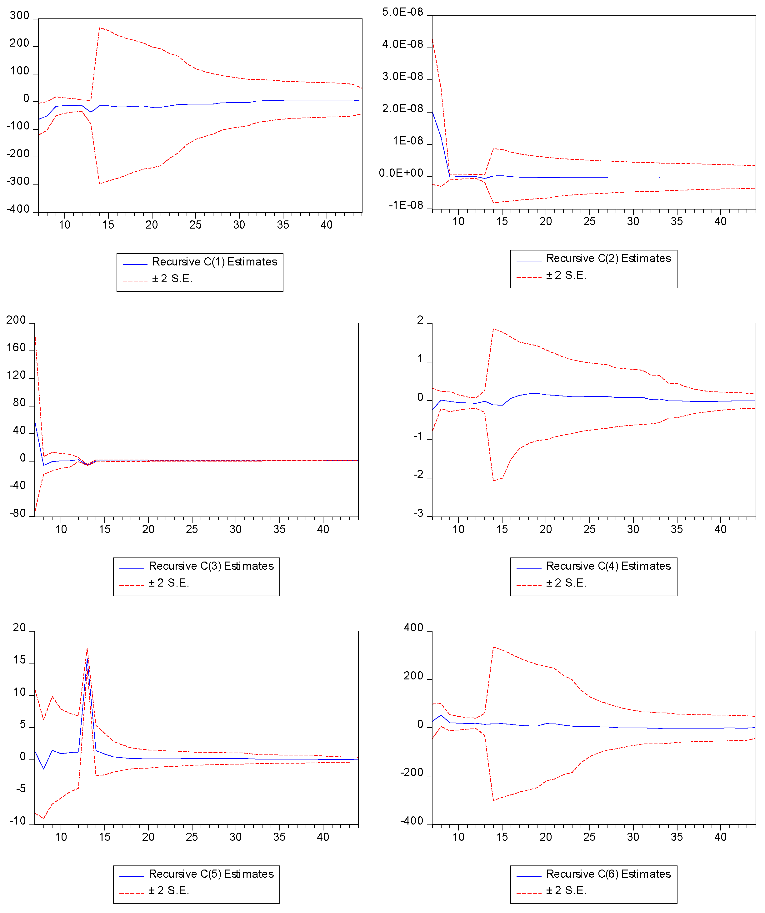
Table 2.
Descriptive Statistics.
| Variables | Mean | Std. Dev. | Skewness | Kurtosis |
|---|---|---|---|---|
| Current ratio | 0.631636 | 0.485922 | 0.962003 | 3.992048 |
| Quick ratio | 1.512334 | 6.253433 | 5.716388 | 35.75535 |
| Cash ratio | 9.964341 | 43.08817 | 4.508002 | 21.82719 |
| Debt ratio | 94.47864 | 123.2578 | 1.717238 | 5.093021 |
| Debt to equity ratio | 55.70757 | 63.82702 | 0.572281 | 1.760132 |
| Return on equity | 14.16220 | 79.67712 | 6.346338 | 41.51864 |
Source: Authors compilation.
Table 3.
Correlations.
| Variables | Current ratio | Quick ratio | Cash ratio | Debt ratio | Debt to equity ratio | Return on equity |
|---|---|---|---|---|---|---|
| Current ratio | 1.00 | |||||
| Quick ratio | 0.200 | 1.00 | ||||
| Cash ratio | 0.666 | 0.543 | 1.00 | |||
| Debt ratio | 0.261 | 0.001 | 0.496 | 1.00 | ||
| Debt to equity ratio | 0.215 | 0.202 | 0.892 | 0.455 | 1.00 | |
| Return on equity | 0.486 | 0.408 | 0.579 | 0.281 | 0.784 | 1.00 |
Source: Authors compilation.
Table 4.
Unit root estimation.
| Variables | Level | 1st Dif. | Level | 1st Diff. | ||
|---|---|---|---|---|---|---|
| Current ratio | 0.000 | - | No Difference Stationary Process | 0.000 | - | No Difference Stationary Process |
| Quick ratio | 0.7587 | 0.0259 | I (1) have no Difference Stationary Process | 0.6825 | 0.0295 | I (1) have no Difference Stationary Process |
| Cash ratio | 0.0005 | - | No Difference Stationary Process | 0.2003 | 0.0041 | I (1) have no Difference Stationary Process |
| Debt ratio | 0.006 | - | No Difference Stationary Process | 0.0007 | - | No Difference Stationary Process |
| Debt to equity ratio | 0.011 | - | No Difference Stationary Process | 0.1911 | 0.000 | I (1) have no Difference Stationary Process |
| Return on equity | 0.051 | 0.000 | I (1) have n Difference Stationary Process | 0.0427 | - | No Difference Stationary Process |
Source: Authors compilation.
Table 5.
Co-Integration estimation.
| Hypothesized No. of C.E. (s) | Eigen Value | Trace Statistics | 0.05 Critical Value | Prob.** |
|---|---|---|---|---|
| None * | 0.515056 | 85.89500 | 95.75366 | 0.1963 |
| At most 1* | 0.394243 | 55.49872 | 69.81889 | 0.3984 |
| At most 2* | 0.309126 | 34.44511 | 47.85613 | 0.4776 |
| At most 3* | 0.249281 | 18.91359 | 29.79707 | 0.4992 |
| At most 4* | 0.108545 | 6.871191 | 15.49471 | 0.5927 |
| At most 5* | 0.047533 | 2.045396 | 3.841466 | 0.1527 |
Source: Authors compilation.
Table 6.
OLS test estimation.
| Variable | Coefficient | Std. Error | t-Statistic | Prob. |
|---|---|---|---|---|
| Current ratio | 2.490649 | 23.10473 | 0.107798 | 0.9147 |
| Quick ratio | -8.42E-11 | 1.76E-09 | -0.047811 | 0.9621 |
| Cash ratio | 1.065902 | 0.246648 | 4.321545 | 0.0001 |
| Debt ratio | -0.006518 | 0.098625 | -0.066088 | 0.9477 |
| Debt to equity ratio | 0.037244 | 0.191049 | 0.194947 | 0.8465 |
Source: Authors compilation.
Table 7.
Heteroscedasticity estimation.
| F-Statistics | 24218.54 | 4.147086 | Prob. F (14,35) | 0.0000 |
| Observed R-Sq. | 43.99791 | 31.19477 | P Chi-Square (14) | 0.0015 |
| Scaled Explain SS | 365.1336 | 40.84318 | P Chi-Square (14) | 0.0000 |
Source: Authors compilation.
Table 8.
Serial lagged estimation.
| F-Statistics | 29.55292 | Prob. F (2,43) | 0.0000 |
| Observed R-Sq. | 27.34487 | P Chi-Square (2) | 0.0000 |
Source: Authors compilation.
Table 9.
Auto Lagged estimation.
| Variable | Coefficient | Std. Error | t-Statistic |
|---|---|---|---|
| Current ratio | 533.8286 | 3.106760 | 1.138440 |
| Quick ratio | 3.10E-18 | 1.161966 | 1.096181 |
| Cash ratio | 0.060835 | 1.075935 | 1.020112 |
| Debt ratio | 0.009727 | 2.137116 | 1.334693 |
| Debt to equity ratio | 0.036500 | 2.389824 | 1.342992 |
Source: Authors compilation.
Table 10.
Ramsey Reset estimation.
| Value | DF | Probability | |
|---|---|---|---|
| t-Statistics | 17.77079 | 37 | 0.0000 |
| F-Statistics | 315.8010 | (1, 37) | 0.0000 |
| Likelihood ratio | 99.2193 | 1 | 0.0000 |
Source: Authors compilation.
Table 11.
GARCH/TARCH estimation.
| Variable | Coefficient | Std. Error | t-Statistic | Prob. |
|---|---|---|---|---|
| Current ratio | 1.682202 | 0.693778 | 2.424699 | 0.0153 |
| Quick ratio | 2.31E-09 | 4.47E-10 | 5.162136 | 0.0000 |
| Cash ratio | 2.112708 | 0.225020 | 9.388994 | 0.0000 |
| Debt ratio | 0.000941 | 0.001054 | 0.893249 | 0.3717 |
| Debt to equity ratio | 0.009071 | 0.002405 | 3.771852 | 0.0002 |
| C | -1.866549 | 0.617014 | -3.025134 | 0.0025 |
| R-Square | 0.7465 | Adjusted R-Square | 0.7552 |
Source: Authors compilation.
Table 12.
PARCH estimation.
| Variable | Coefficient | Std. Error | t-Statistic | Prob. |
|---|---|---|---|---|
| Current ratio | -0.223873 | 0.218449 | -1.024827 | 0.3054 |
| Quick ratio | -1.04E-10 | 4.39E-11 | -2.361792 | 0.0182 |
| Cash ratio | 2.789148 | 0.056680 | 49.20829 | 0.0000 |
| Debt ratio | 7.40E-05 | 0.000502 | 0.147345 | 0.8829 |
| Debt to equity ratio | 0.004119 | 0.001157 | 3.560372 | 0.0004 |
| C | -0.032296 | 0.177181 | -0.182276 | 0.8554 |
| R-Square | 0.5555 | Adjusted R-Square | 0.76223 |
Source: Authors compilation.
Disclaimer/Publisher’s Note: The statements, opinions and data contained in all publications are solely those of the individual author(s) and contributor(s) and not of MDPI and/or the editor(s). MDPI and/or the editor(s) disclaim responsibility for any injury to people or property resulting from any ideas, methods, instructions or products referred to in the content. |
© 2025 by the authors. Licensee MDPI, Basel, Switzerland. This article is an open access article distributed under the terms and conditions of the Creative Commons Attribution (CC BY) license (http://creativecommons.org/licenses/by/4.0/).
Copyright: This open access article is published under a Creative Commons CC BY 4.0 license, which permit the free download, distribution, and reuse, provided that the author and preprint are cited in any reuse.


