
Submitted:
13 February 2025
Posted:
17 February 2025
You are already at the latest version
Abstract
Cooperative, Connected, and Automated Mobility (CCAM) is set to play a key role in the future of transportation, contributing to the achievement of sustainable development goals. Moreover, Artificial Intelligence (AI), a transformative technology with applications across various industries, can significantly enhance CCAM operations. Additionally, passenger demand forecasting, a critical aspect of mobility research, will become even more essential as CCAM adoption continues to grow in the next years. Therefore, the present research study in order to deal with the issue of passenger demand forecasting in CCAM, proposes the Principal Component Random Forest (PCRF) methodology, which is based on AI as it leverages a well-established statistical methodology such as the Principal Components Analysis with a flagship traditional machine learning technique, which is Random Forest. The application of PCRF in four European pilot sites within the EU-funded SHOW project demonstrated its high accuracy and effectiveness.
Keywords:
machine learning
; principal component analysis
; random forest
; passenger demand forecasting
; urban mobility
; automated mobility
1. Introduction
Undoubtedly, Cooperative, Connected, and Automated Mobility (CCAM) is a groundbreaking technology [1] in the contemporary society and a promising solution for advancing the Sustainable Development Goals (SDGs) [2]. In particular, SDG 11: Sustainable Cities and Communities and SDG 13: Climate Action could greatly benefit from this transformative mode of transportation [3] for people and goods, as Automated Vehicles (AVs) primarily rely on electricity [4]. Even more significantly, integrating automated mobility with public urban transportation could contribute to a greener environment by reducing reliance on private cars, thereby decreasing traffic congestion and its associated environmental impact [5].
It is undeniable that Artificial Intelligence (AI) and Big Data (BD) are revolutionizing factors in the modern business environment [6], demonstrating their prowess across various sectors, including healthcare [7], agriculture [8], energy [9], tourism [10] and Industry 5.0 [11]. More specifically, a recent literature review (to be added) highlights the potential of AI in the CCAM sector. Hence, recent research efforts leveraging AI and BD in CCAM [12] are continuously increasing, enhancing the benefits for commuters by providing valuable solutions to common urban transportation challenges, such as Estimated Time of Arrival prediction [13] and Accident Detection [14].
Passenger demand forecasting is one of the primary concerns in transportation research [15], both for scheduled and unscheduled transportation. Indeed, an accurate prediction of passenger demand can facilitate optimal resource planning and allocation [16] across various transportation modes, including airplanes [17], ships [18], buses [19], and taxis [20]. This, in turn, can lead to economic benefits for transport operators [21], whether public or private.
According to the aforementioned, it is imperative to find a viable solution to the existing challenge of accurately forecasting passenger demand in CCAM by leveraging advanced technological tools such as Machine Learning (ML) and robust statistical analysis. For this reason, the suggested methodology Principal Component Random Forest (PCRF), combines statistical and ML techniques, namely, the Principal Component Analysis (PCA) and Random Forest (RF), to predict daily passenger demand for automated vehicles operating in both scheduled and non-scheduled transportation services, using real data from four different pilot sites across Europe of the SHOW project 1.
The rest of the article is organized as follows. Section 2 describes the related work of the research field, while Section 3 presents the proposed methodology, PCRF, for passenger demand forecasting. Section 4 discusses the experimental results of applying PCRF to five real-life datasets and finally, Section 5 summarizes the key conclusions of this research.
2. Related Work
As mentioned in the Introduction, Passenger Demand Forecasting in urban transportation plays a prominent role for the transport operators . Indeed, there are various research studies in the literature that have attempted to address this challenge efficiently. A recent literature review emphasizes the importance of incorporating spatial and temporal characteristics to enhance the accuracy of passenger demand prediction [22]. According to the same systematic review, related works in this field primarily fall into two main categories: statistical-based methodologies and modern AI-based approaches. The following paragraphs present some representative studies from both categories.
Starting with the statistical-based category, Xue et al. [23] proposed a methodology utilizing time-series models and the Interactive Multiple Model algorithm to predict short-term passenger demand for a specific bus route in Shenzhen, China. Their results demonstrated the accuracy of the proposed approach when applied to a four-month dataset, achieving a Mean Absolute Percentage Error (MAPE) below 10%. Similarly, Tang et al. [24] suggested a statistical approach based on seasonal decomposition to predict short-term subway ridership of the Chongqing Rail Transit in China. Their approach achieved high accuracy, with a MAPE below 8%. Finally, Tao et al. [25] examined the impact of weather on passenger demand by incorporating weather-related variables into a statistical SARIMAX model. Using a dataset of hourly bus rides in Brisbane, Australia, their study demonstrated a strong correlation between real-time weather variables—such as temperature and wind speed—and passenger demand.
Continuing with the more advanced and sophisticated AI-based approaches, Hao et al. [26] employed a deep learning model that combines sequence-to-sequence learning with an attention mechanism for short-term passenger demand prediction in metro stations. Their study used data from two major Singapore metro stations—Raffles Place MRT and Clarke Quay MRT. The proposed methodology proved highly effective, achieving significantly lower prediction errors compared to traditional ML benchmarks. Similarly, Liu et al. [27] to predict short-term passenger demand in metro of Taipei, Taiwan, used a deep long short-term memory neural network, incorporating weather variables such as temperature and wind speed. The results indicated that the proposed methodology is very accurate, achieving a MAPE approximately 5%, although the inclusion of weather variables did not lead to a significant improvement in prediction accuracy. Finally, Liu et al. [28] integrated decision trees for feature engineering with a deep learning network to forecast passenger demand for public transport buses in Nanjing, China. Their results demonstrated superior performance compared to other neural network-based approaches.
It is evident from the aforementioned discussion that this study differentiates itself from related works, as it represents the first attempt to predict daily passenger demand in the CCAM, which is a unique mode of transportation with distinct characteristics compared to conventional transport systems, using five real-life datasets. Moreover, to the best of our knowledge, the proposed PCRF methodology, which is an iterative approach combining PCA with RF, is being applied for the first time in a demand forecasting problem, and more specifically for passenger demand forecasting in CCAM for urban transportation.
3. Methodology
As mentioned in Introduction, a new methodology is proposed in the present study to predict the daily passenger demand in CCAM. The proposed PCRF methodology adopts an iterative approach and is based on statistical and ML methodologies. The combination of statistical and ML methodologies is followed in this research, as it leads very frequently to better forecasting accuracy according to the literature [29,30,31,32]. In particular, the proposed methodology leverages i) the statistical methodology of PCA that reduces the variable dimensionality [33,34], thus providing reduced variance [35] with ii) the flagship ML methodology of Random Forest that is extremely efficient in many classification and regression problems in terms of prediction accuracy as proved from the literature of various disciplines [36,37].
PCA [38,39] transforms high-dimensional data into a smaller set of uncorrelated variables called principal components. It works by identifying directions of maximum variance in the data and projecting it onto these new axes, preserving as much information as possible while reducing complexity. Random Forest [40,41] is a powerful ensemble learning algorithm that builds multiple decision trees and combines their outputs to improve accuracy and reduce overfitting. It works by training each tree on a random subset of the data and averaging their predictions (for regression) or using majority voting (for classification). The overall methodology, which is based on the two aforementioned methodologies, is presented in detail in the following paragraphs.
The first step of the PCRF constitutes the input of historical data of daily passenger demand. A very simple approach is followed in this study regarding the input data as the proposed algorithm uses as input only the historical previous values for a specific route or a specific region. This consideration is met very frequently in the literature for similar timeseries problems, as keeps the simplicity of a methodology accompanied by very accurate results [42,43,44].
The next step of PCRF includes the data preprocessing by taking the input from the first step and by performing the required preprocessing of the historical demand, which constitutes a time-series, in order to transform [45] it in a form suitable for the chosen ML algorithm, which is Random forest. Thus, the historical demand is transformed in such a way that each of the previous values (passenger daily demand in this case) is in essence a feature for the algorithms. That way, the training of the algorithm considers appropriately the chronological order (i.e., the future values are not used for the training of the past values), and the training does not have the bias problem [37,45].
After the data preprocessing, which described in detail above, the third step of the methodology is the training of the Random Forest algorithm, which takes place in the corresponding training set. At this point, it is worth-noting the splitting of the datasets in three parts, the training set, in which the algorithm is trained iteratively, the validation set, in which the fine-tuning of the algorithm is taken place and the test set, which constitutes the last. The splitting of the datasets in these three parts follows the best practices of the literature [46]. In the next paragraphs, the fine-tuning of the methodology in the validation set is analyzed.
The selection of the optimal number of historical passenger demand values constitutes the fourth step of the proposed methodology. In order to do this selection, as mentioned before, the validation set of each sample is used. It is worth-mentioning at this point, that the maximum number of historical passenger demand values depends on the dataset size. Therefore, and due to the differentiation in the size of the five datasets used, as presented in the Results Section, a different range of historical values is considered in this step for the datasets. For the selection of the optimal number of previous days the Root Mean Square Error (RMSE) evaluation metric is used and this consideration is aligned with the respective literature [47].
After the selection of the optimal previous days, the fifth step of the methodology contains the PCA conduction in order to reduce the number of features and create new uncorrelated variables [38]. It is worth mentioning that the dataset in which PCA is performed consists of the historical values defined in the previous step as columns and each row corresponds to a specific date. As previously, for the procedure of the algorithm fine-tuning, namely the selection of the number of components is performed in the validation set considering the RMSE evaluation criterion [47].
Next, the proposed algorithm checks if the transformed values from the PCA achieve improved performance in comparison with the original dataset. Therefore, depending on the previous decision of the algorithm, the procedure continues with the original or the transformed/reduced from the PCA dataset. Since, this decision is essentially, a fine-tuning of the methodology is conducted as with all the fine-tuning steps presented in the validation set and the RMSE evaluation criterion decides with which dataset the algorithm will continue.
The final step of the fine-tuning procedures corresponds to the tuning of the hyper parameters of Random Forest (number of trees/features per split), considering among others the values suggested by Breiman [40] for these hyper parameters. Once again, the tuning of the Random Forest hyper-parameters is performed in the validation set and the criterion for the fine-tuning is RMSE.
Finally, considering the small size of the five available datasets (more details regarding the dataset size are provided in the Results Section), the well-established in time-series problems and simple approach of next-step forecasting [42,48] is applied. Hence, the derived model predicts the passenger demand for the next day only from the previous historical values. The overall procedure of the proposed PCRF methodology is depicted in Figure 1.
3.1. Evaluation Metrics
This subsection presents the evaluation metrics used in this study to validate the proposed PCRF methodology. In line with the literature [49], well-established evaluation metrics for regression problems are employed, including Mean Absolute Error (MAE), Median Absolute Error (MdAE), and RMSE, along with their normalized versions [42]. The following formulas illustrate how these metrics are computed:
where is the error between actual and predicted values and n is the number of predicted demand values.
a metric more robust and resilient against outliers compared to
a stricter metric than the , as it penalizes the big errors more
where y is the vector of actual passenger demand values
The last three normalized metrics are very useful for ML regression problems, as they provide insights regarding the error magnitude and the general performance of the methodologies regardless of the research field and the value level.
4. Results
This section presents the results of the proposed PCRF methodology for daily passenger demand forecasting across the following pilot sites:
- Tampere, Finland (two different running phases)
- Frankfurt, Germany
- Carinthia, Austria
- Trikala, Greece
4.1. Tampere 1st phase
The first period of the Tampere pilot site, which includes passenger demand data, spans from 05/01/2022 to 10/03/2022. During this period, there were 44 operational days. Of these, 34 days were used for the training set, while five days were allocated for both the validation and test sets. The forecasting results are illustrated in Figure 2, where the ability of the proposed methodology to capture passenger demand magnitude can be observed.
4.2. Tampere 2nd phase
The second period used for demand forecasting at the Tampere pilot site is significantly longer than the first, spanning approximately six months from 09/01/2023 to 30/06/2023. Consequently, the number of operational days in this period is nearly three times higher than in the first, increasing from 44 to 117 days. As expected, the training, validation, and testing sets are also larger, consisting of 77, 20, and 20 days, respectively. Finally, as shown in Figure 3, the forecasting results indicate that, in addition to accurately capturing passenger demand magnitude, the proposed methodology also effectively captures demand patterns due to the larger dataset.
4.3. Frankfurt
In Frankfurt, passenger data is available for 159 operational days from 01/12/2022 to 30/06/2023. For this pilot site, the dataset was divided into 99 days for training, 30 days for validation, and 30 days for testing. Finally, as shown in Figure 4, the forecasting results demonstrate that the proposed methodology effectively captures the passenger demand pattern.
4.4. Carinthia
In Carinthia, passenger data is available for only 29 operational days from 21/09/2021 to 12/11/2021. As expected, the dataset for training, validation, and testing is relatively small, consisting of 19, 5, and 5 days, respectively. Figure 5 presents the actual and forecasted passenger demand values, demonstrating that the proposed methodology successfully captures the passenger demand levels.
4.5. Trikala
In Trikala, passenger data is available for 38 operational days from 01/02/2024 to 29/03/2024. Given the relatively small dataset, the training, validation, and test sets consist of 28, 5, and 5 days, respectively. As shown in Figure 6, the PCRF methodology successfully captured the passenger demand level.
4.6. Evaluation Results
Table 1 presents a summary of the results across all pilot sites based on the evaluation metrics analyzed in subSection 3.1. As shown, the proposed forecasting methodology achieved consistently strong performance, with error rates ranging from below 6% (NMdAE for Carinthia) to below 30% (NRMSE for Trikala). This outcome is particularly promising, given the limited dataset size for most pilot sites, further demonstrating the effectiveness of the proposed approach.
4.7. Comparative Results
As a final step to validate the proposed PCRF methodology and in accordance with Hyndman’s guidelines [50] for methodology benchmarking, Table 2 presents a comparison of the proposed approach with baseline forecasting methods such as Naïve, Average, and Drift. Since the primary focus of this table is comparison, only the normalized versions of MAE, MdAE, and RMSE are displayed. This is because a method that achieves the best results in the normalized metric (e.g NMAE) will also yield the best results in the base metric (e.g. MAE), making the inclusion of non-normalized metrics redundant."
It is obvious from Table 2 that the proposed methodology performed better than the baseline methodologies of Naive, Average, and Drift. More particularly, the suggested PCRF methodology was the best forecasting methodology according to the evaluation metrics 8 out of 15 times (3 evaluation metrics for the five datasets). The superiority of the suggested forecasting methodology against the baseline methodologies is also proven from the fact that in the largest datasets (Frankfurt, Tampere 2nd phase, and Tampere 1st phase with 159, 127, and 44 records respectively) has the best results 7 out of 9 times. Finally, another point indicating the superiority of the proposed PCRF methodology is that in the three largest datasets, PCRF achieved the best NRMSE, which constitutes the normalized version of the most rigorous evaluation metric as described in the evaluation metrics subsection.
5. Conclusions
The present article introduced a novel iterative methodology for passenger demand prediction in CCAM, leveraging statistical and machine learning methodologies, such as PCA and Random Forest. The application of the proposed PCRF methodology to five real-life datasets from four pilot sites demonstrated its reliability and robustness, regarding forecasting accuracy, even when working with limited data. Additionally, comparative analysis against baseline forecasting methods—widely recognized for their simplicity and efficiency with small datasets—highlighted the superiority of the proposed approach and its potential.
As future work, the suggested PCRF methodology will be further enhanced by incorporating features known to influence passenger demand in urban mobility, such as weather conditions and various spatiotemporal factors. Moreover, a crucial future action toward the generalizability of the PCRF methodology will be its application to larger CCAM datasets, allowing for comparisons with more sophisticated and complex AI methodologies, including deep learning approaches and algorithms from the boosting family.
Author Contributions
Conceptualization, G.S.; methodology, G.S.; software, G.S.; validation, G.S.; formal analysis, G.S.; investigation, G.S.; data curation, G.S.; writing—original draft preparation, G.S.; writing—review and editing, G.S.; visualization, G.S.; supervision, A.L.; project administration, A.L. and K.V.; funding acquisition, K.V. and D.T. All authors have read and agreed to the published version of the manuscript.
Funding
This work was partially funded by the European’s Union Horizon 2020 Research and Innovation Program through SHared automation Operating models for Worldwide adoption (SHOW) under Grant Agreement No. 875530.
Data Availability Statement
Data is unavailable due to privacy or ethical restrictions
Conflicts of Interest
The authors declare no conflicts of interest. The funders had no role in the design of the study; in the collection, analyses, or interpretation of data; in the writing of the manuscript; or in the decision to publish the results.
References
- Gruyer, D.; Orfila, O.; Glaser, S.; Hedhli, A.; Hautière, N.; Rakotonirainy, A. Are connected and automated vehicles the silver bullet for future transportation challenges? Benefits and weaknesses on safety, consumption, and traffic congestion. Frontiers in sustainable cities 2021, 2, 607054. [Google Scholar] [CrossRef]
- Hák, T.; Janoušková, S.; Moldan, B. Sustainable Development Goals: A need for relevant indicators. Ecological indicators 2016, 60, 565–573. [Google Scholar] [CrossRef]
- Chehri, A.; Mouftah, H.T. Autonomous vehicles in the sustainable cities, the beginning of a green adventure. Sustainable Cities and Society 2019, 51, 101751. [Google Scholar] [CrossRef]
- Taiebat, M.; Brown, A.L.; Safford, H.R.; Qu, S.; Xu, M. A review on energy, environmental, and sustainability implications of connected and automated vehicles. Environmental science & technology 2018, 52, 11449–11465. [Google Scholar]
- Lazarus, J.; Shaheen, S.; Young, S.E.; Fagnant, D.; Voege, T.; Baumgardner, W.; Fishelson, J.; Sam Lott, J. Shared automated mobility and public transport; Springer, 2018.
- Obschonka, M.; Audretsch, D.B. Artificial intelligence and big data in entrepreneurship: a new era has begun. Small Business Economics 2020, 55, 529–539. [Google Scholar] [CrossRef]
- Benke, K.; Benke, G. Artificial intelligence and big data in public health. International journal of environmental research and public health 2018, 15, 2796. [Google Scholar] [CrossRef]
- Wolfert, S.; Ge, L.; Verdouw, C.; Bogaardt, M.J. Big data in smart farming–a review. Agricultural systems 2017, 153, 69–80. [Google Scholar] [CrossRef]
- Li, J.; Herdem, M.S.; Nathwani, J.; Wen, J.Z. Methods and applications for Artificial Intelligence, Big Data, Internet of Things, and Blockchain in smart energy management. Energy and AI 2023, 11, 100208. [Google Scholar] [CrossRef]
- Samara, D.; Magnisalis, I.; Peristeras, V. Artificial intelligence and big data in tourism: a systematic literature review. Journal of Hospitality and Tourism Technology 2020, 11, 343–367. [Google Scholar] [CrossRef]
- Rijwani, T.; Kumari, S.; Srinivas, R.; Abhishek, K.; Iyer, G.; Vara, H.; Dubey, S.; Revathi, V.; Gupta, M. Industry 5.0: a review of emerging trends and transformative technologies in the next industrial revolution. International Journal on Interactive Design and Manufacturing (IJIDeM) 2024, 1–13. [Google Scholar] [CrossRef]
- Spanos, G.; Siomos, A.; Schmidt, C.; Tygesen, M.; Salanova, J.M.; Rodrigues, F.; Papadopoulos, A.; Antypas, E.; Sersemis, A.; Gemou, M.; et al. Services for Connected, Cooperated, and Automated Mobility based on Big Data and Artificial Intelligence: The SHOW project paradigm. Open Research Europe 2025, 5, 24. [Google Scholar] [CrossRef]
- Antypas, E.; Spanos, G.; Lalas, A.; Votis, K.; Tzovaras, D. A time-series approach for estimated time of arrival prediction in autonomous vehicles. Transportation research procedia 2024, 78, 166–173. [Google Scholar] [CrossRef]
- Papadopoulos, A.; Sersemis, A.; Spanos, G.; Lalas, A.; Liaskos, C.; Votis, K.; Tzovaras, D. Lightweight accident detection model for autonomous fleets based on GPS data. Transportation research procedia 2024, 78, 16–23. [Google Scholar] [CrossRef]
- Banister, D. Sustainable transport: Challenges and opportunities. Transportmetrica 2007, 3, 91–106. [Google Scholar] [CrossRef]
- Banerjee, N.; Morton, A.; Akartunalı, K. Passenger demand forecasting in scheduled transportation. European Journal of Operational Research 2020, 286, 797–810. [Google Scholar] [CrossRef]
- Higgoda, R.; Madurapperuma, M. Dynamic Nexus between Air-Transportation and Economic Growth: A Systematic Literature Review. Journal of Transportation Technologies 2019, 9, 156–170. [Google Scholar] [CrossRef]
- Xu, M.; Ma, X.; Zhao, Y.; Qiao, W. A Systematic Literature Review of Maritime Transportation Safety Management. Journal of Marine Science and Engineering 2023, 11, 2311. [Google Scholar] [CrossRef]
- Sogbe, E.; Susilawati, S.; Pin, T.C. Scaling up public transport usage: a systematic literature review of service quality, satisfaction and attitude towards bus transport systems in developing countries. Public Transport 2024, 1–44. [Google Scholar] [CrossRef]
- Lyu, T.; Wang, P.S.; Gao, Y.; Wang, Y. Research on the big data of traditional taxi and online car-hailing: A systematic review. Journal of Traffic and Transportation Engineering (English Edition) 2021, 8, 1–34. [Google Scholar] [CrossRef]
- Zachariah, R.A.; Sharma, S.; Kumar, V. Systematic review of passenger demand forecasting in aviation industry. Multimedia tools and applications 2023, 82, 46483–46519. [Google Scholar] [CrossRef]
- Nithin, K.S.; Mulangi, R.H. Spatio-Temporal Factors Affecting Short-Term Public Transit Passenger Demand Prediction: A Review. In Proceedings of the International Conference on Transportation Planning and Implementation Methodologies for Developing Countries. Springer, 2022, pp. 421–430.
- Xue, R.; Sun, D.; Chen, S. Short-term bus passenger demand prediction based on time series model and interactive multiple model approach. Discrete Dynamics in Nature and Society 2015, 2015, 682390. [Google Scholar] [CrossRef]
- Tang, J.; Zuo, A.; Liu, J.; Li, T. Seasonal decomposition and combination model for short-term forecasting of subway ridership. International Journal of Machine Learning and Cybernetics 2022, 13, 145–162. [Google Scholar] [CrossRef]
- Tao, S.; Corcoran, J.; Rowe, F.; Hickman, M. To travel or not to travel:‘Weather’is the question. Modelling the effect of local weather conditions on bus ridership. Transportation research part C: emerging technologies 2018, 86, 147–167. [Google Scholar] [CrossRef]
- Hao, S.; Lee, D.H.; Zhao, D. Sequence to sequence learning with attention mechanism for short-term passenger flow prediction in large-scale metro system. Transportation Research Part C: Emerging Technologies 2019, 107, 287–300. [Google Scholar] [CrossRef]
- Liu, L.; Chen, R.C.; Zhu, S. Impacts of weather on short-term metro passenger flow forecasting using a deep LSTM neural network. Applied Sciences 2020, 10, 2962. [Google Scholar] [CrossRef]
- Liu, Y.; Lyu, C.; Liu, X.; Liu, Z. Automatic feature engineering for bus passenger flow prediction based on modular convolutional neural network. IEEE Transactions on Intelligent Transportation Systems 2020, 22, 2349–2358. [Google Scholar] [CrossRef]
- Koutroumanidis, T.; Sylaios, G.; Zafeiriou, E.; Tsihrintzis, V.A. Genetic modeling for the optimal forecasting of hydrologic time-series: Application in Nestos River. Journal of Hydrology 2009, 368, 156–164. [Google Scholar] [CrossRef]
- Caliwag, A.C.; Lim, W. Hybrid VARMA and LSTM method for lithium-ion battery state-of-charge and output voltage forecasting in electric motorcycle applications. Ieee Access 2019, 7, 59680–59689. [Google Scholar] [CrossRef]
- Hong, J.; Wang, Z.; Chen, W.; Wang, L.Y.; Qu, C. Online joint-prediction of multi-forward-step battery SOC using LSTM neural networks and multiple linear regression for real-world electric vehicles. Journal of Energy Storage 2020, 30, 101459. [Google Scholar] [CrossRef]
- Athanasakis, E.; Spanos, G.; Papadopoulos, A.; Lalas, A.; Votis, K.; Tzovaras, D. a Comprehensive Leakage-Free Forecasting Pipeline for Segmented Time Series: Application to Cross-Trip State-of-Charge Prediction in Automated Electric Vehicles. IEEE Transactions on Intelligent Vehicles 2024. [Google Scholar] [CrossRef]
- Greenacre, M.; Groenen, P.J.; Hastie, T.; d’Enza, A.I.; Markos, A.; Tuzhilina, E. Principal component analysis. Nature Reviews Methods Primers 2022, 2, 100. [Google Scholar] [CrossRef]
- Spanos, G.; Giannoutakis, K.M.; Votis, K.; Viaño, B.; Augusto-Gonzalez, J.; Aivatoglou, G.; Tzovaras, D. A lightweight cyber-security defense framework for smart homes. In Proceedings of the 2020 International Conference on INnovations in Intelligent SysTems and Applications (INISTA). IEEE, 2020, pp. 1–7.
- James, G.; Witten, D.; Hastie, T.; Tibshirani, R.; et al. An introduction to statistical learning; Vol. 112, Springer, 2013.
- Antoniadis, A.; Lambert-Lacroix, S.; Poggi, J.M. Random forests for global sensitivity analysis: A selective review. Reliability Engineering & System Safety 2021, 206, 107312. [Google Scholar]
- Aivatoglou, G.; Anastasiadis, M.; Spanos, G.; Voulgaridis, A.; Votis, K.; Tzovaras, D.; Angelis, L. A RAkEL-based methodology to estimate software vulnerability characteristics & score-an application to EU project ECHO. Multimedia Tools and Applications 2022, 81, 9459–9479. [Google Scholar]
- Jolliffe, I.T. Principal component analysis for special types of data; Springer, 2002.
- Abdi, H.; Williams, L.J. Principal component analysis. Wiley interdisciplinary reviews: computational statistics 2010, 2, 433–459. [Google Scholar] [CrossRef]
- Breiman, L. Random forests. Machine learning 2001, 45, 5–32. [Google Scholar] [CrossRef]
- Parmar, A.; Katariya, R.; Patel, V. A review on random forest: An ensemble classifier. In Proceedings of the International conference on intelligent data communication technologies and internet of things (ICICI) 2018. Springer, 2019, pp. 758–763.
- Polymeni, S.; Pitsiavas, V.; Spanos, G.; Matthewson, Q.; Lalas, A.; Votis, K.; Tzovaras, D. Toward sustainable mobility: AI-enabled automated refueling for Fuel Cell Electric Vehicles. Energies 2024, 17, 4324. [Google Scholar] [CrossRef]
- Wang, W.c.; Chau, K.w.; Xu, D.m.; Chen, X.Y. Improving forecasting accuracy of annual runoff time series using ARIMA based on EEMD decomposition. Water Resources Management 2015, 29, 2655–2675. [Google Scholar] [CrossRef]
- Mahjoub, S.; Chrifi-Alaoui, L.; Marhic, B.; Delahoche, L. Predicting energy consumption using LSTM, multi-layer GRU and drop-GRU neural networks. Sensors 2022, 22, 4062. [Google Scholar] [CrossRef]
- Brownlee, J. Introduction to time series forecasting with python: how to prepare data and develop models to predict the future; Machine Learning Mastery, 2017.
- Xu, Y.; Goodacre, R. On splitting training and validation set: a comparative study of cross-validation, bootstrap and systematic sampling for estimating the generalization performance of supervised learning. Journal of analysis and testing 2018, 2, 249–262. [Google Scholar] [CrossRef]
- Zhou, J.; Shi, J.; Li, G. Fine tuning support vector machines for short-term wind speed forecasting. Energy Conversion and Management 2011, 52, 1990–1998. [Google Scholar] [CrossRef]
- Suradhaniwar, S.; Kar, S.; Durbha, S.S.; Jagarlapudi, A. Time series forecasting of univariate agrometeorological data: a comparative performance evaluation via one-step and multi-step ahead forecasting strategies. Sensors 2021, 21, 2430. [Google Scholar] [CrossRef]
- Hyndman, R.J.; Koehler, A.B. Another look at measures of forecast accuracy. International journal of forecasting 2006, 22, 679–688. [Google Scholar] [CrossRef]
- Hyndman, R. Forecasting: principles and practice; OTexts, 2018.
| 1 |
Figure 1.
PCRF methodology

Figure 2.
Tampere (1st period) Forecasting Results
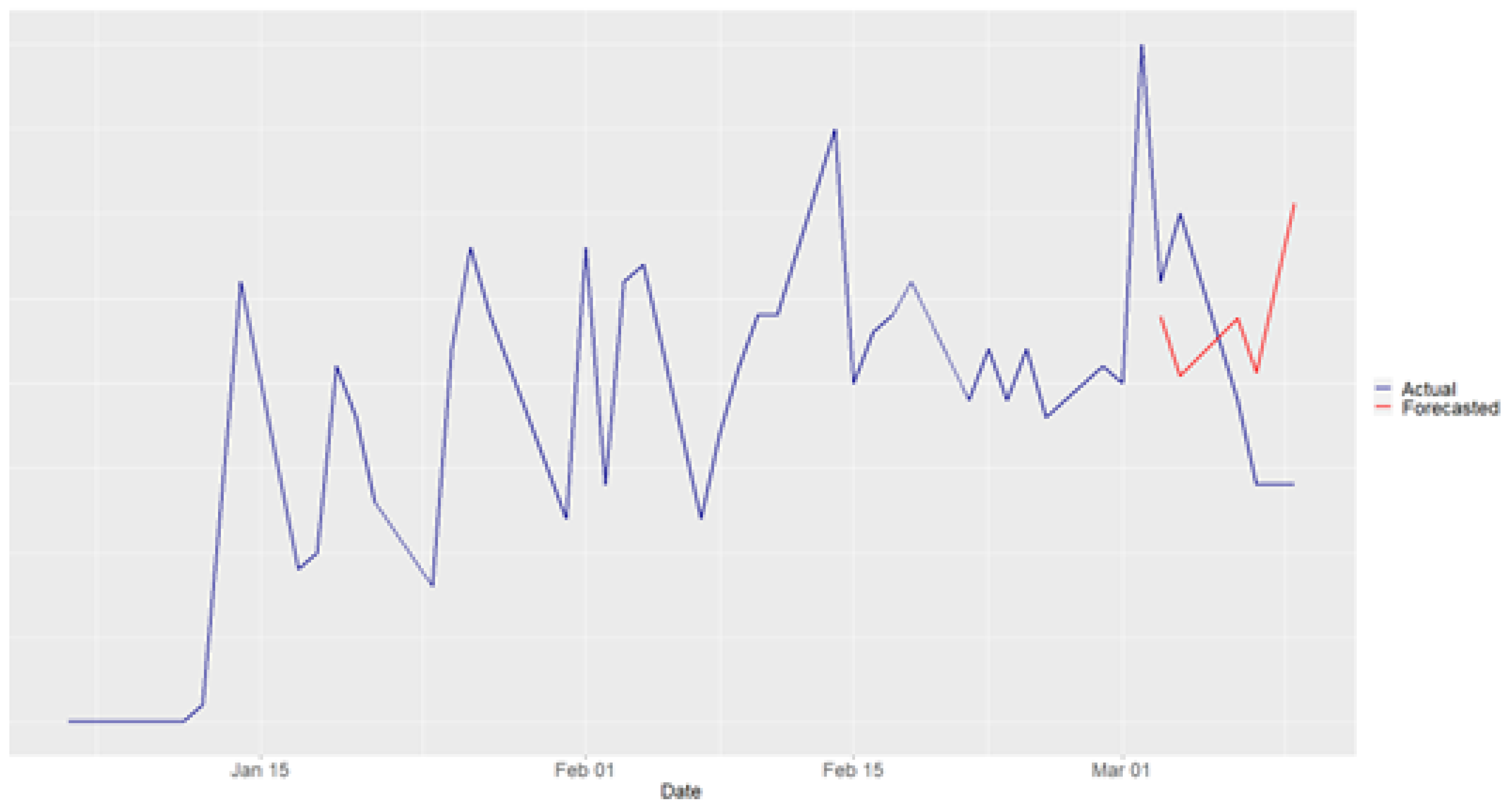
Figure 3.
Tampere (2nd period) Forecasting Results
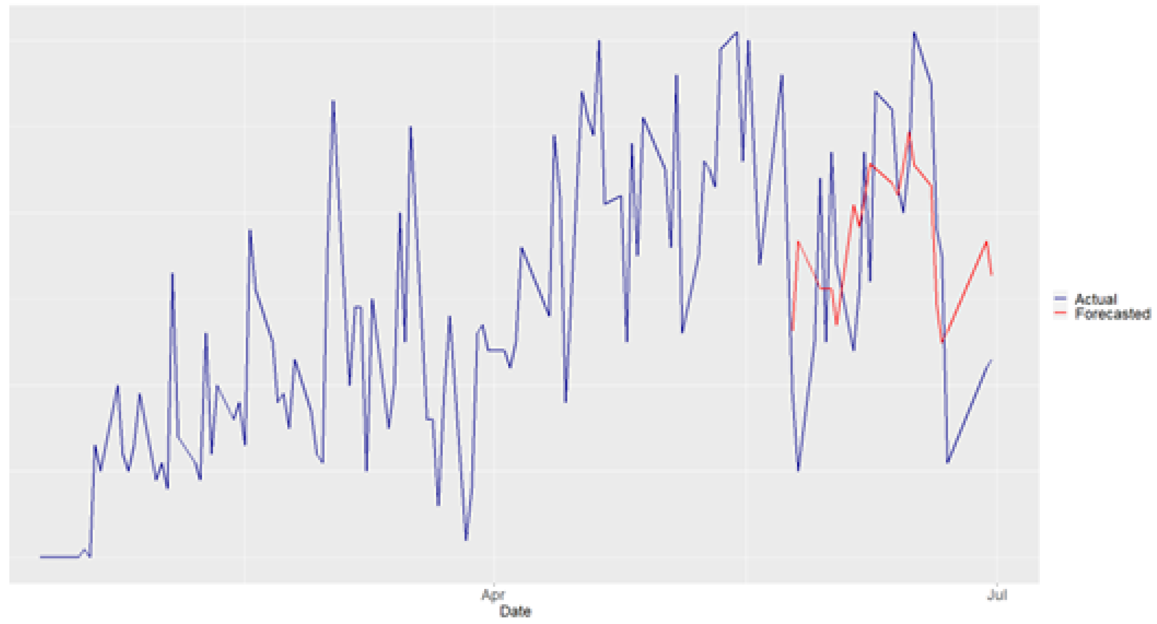
Figure 4.
Frankfurt Forecasting Results
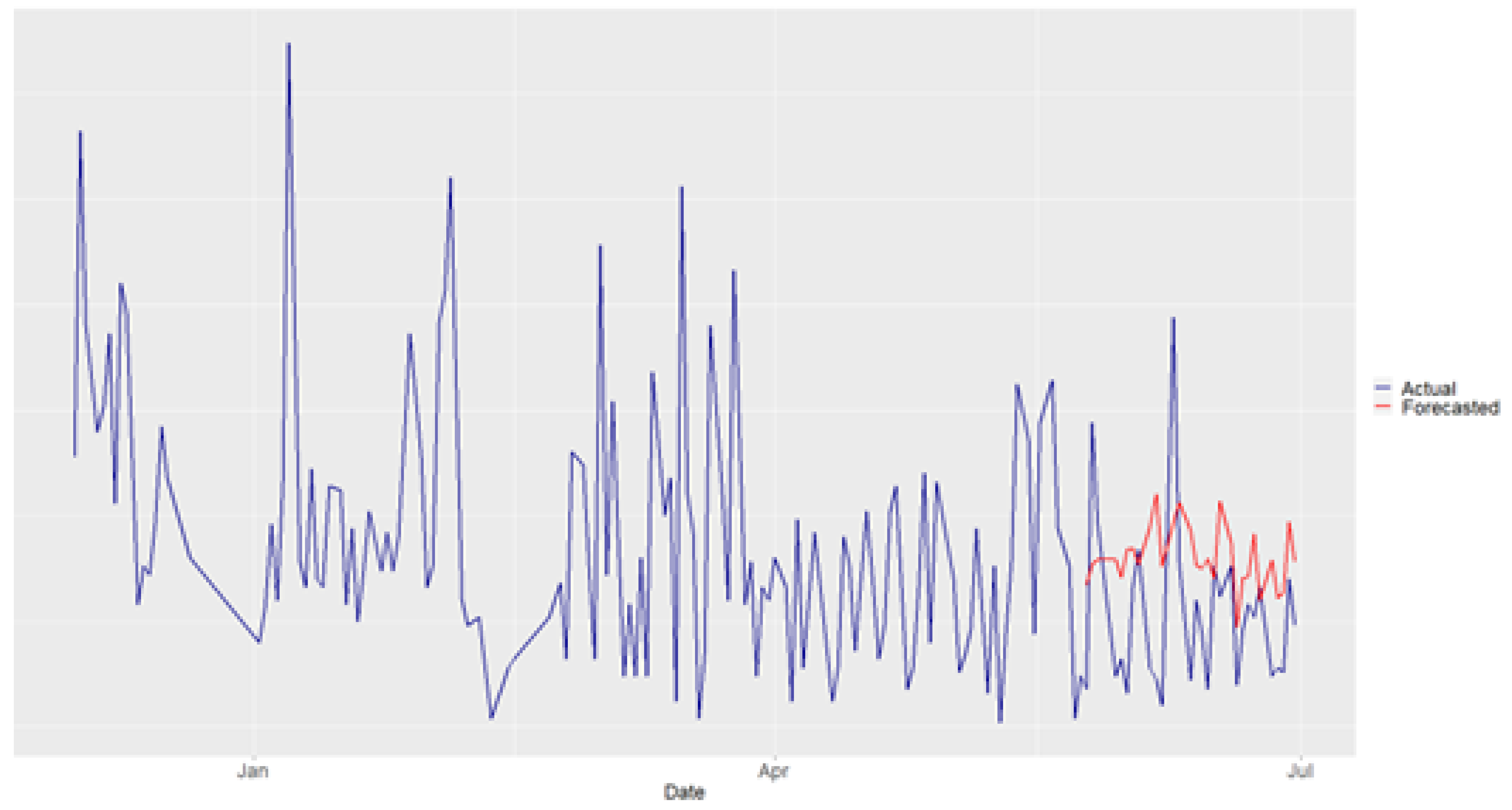
Figure 5.
Carinthia Forecasting Results
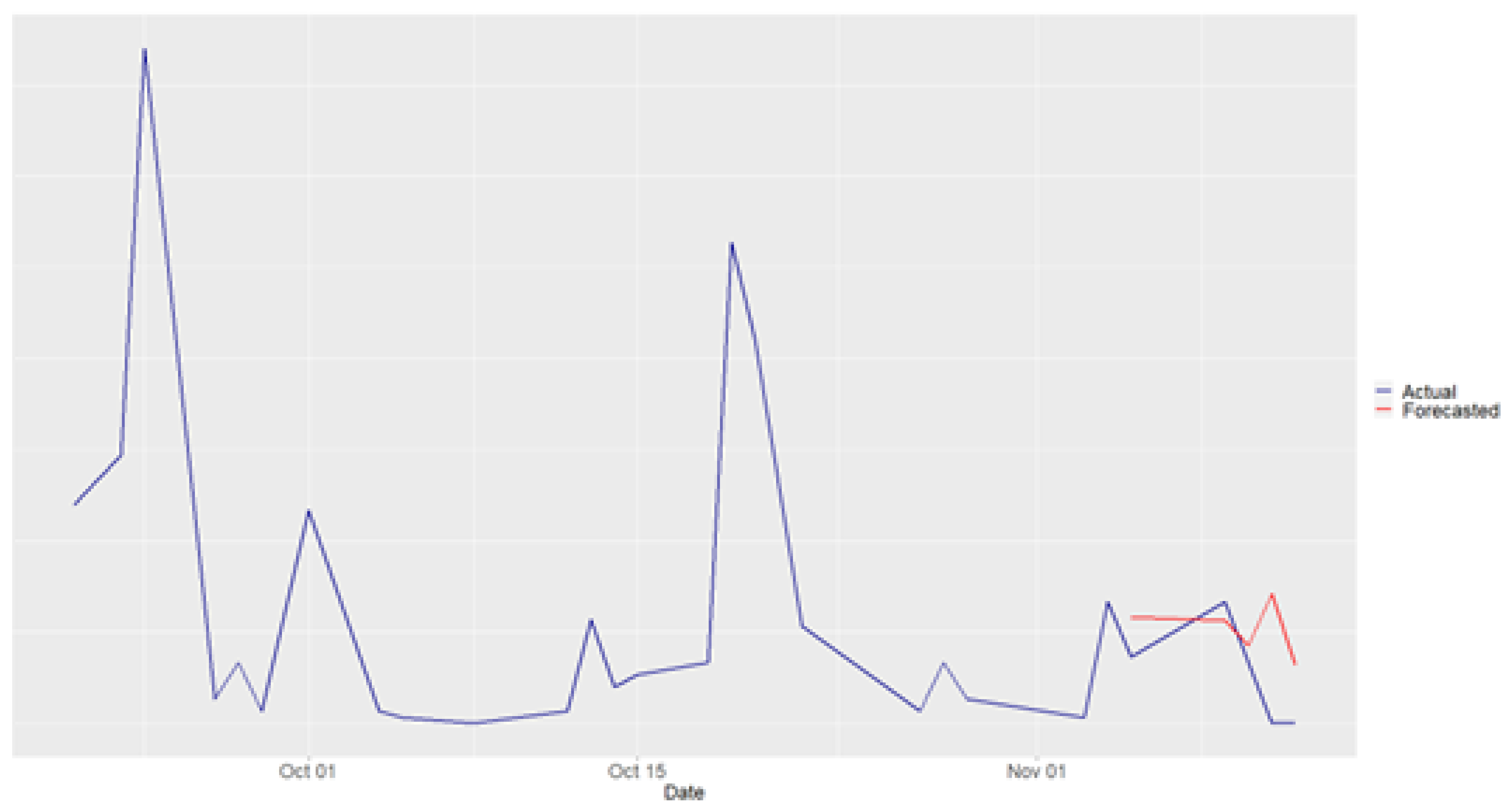
Figure 6.
Trikala Forecasting Results


Table 1.
Summary of the evaluation results for all pilot sites.
| MAE | MdAE | RMSE | NMAE | NMdAE | NRMSE | |
|---|---|---|---|---|---|---|
| Tampere (1st period) | 5.4 | 4.08 | 6.03 | 13.50% | 10.20% | 15.10% |
| Tampere (2nd period) | 10.55 | 10.03 | 12.98 | 17.30% | 16.40% | 21.30% |
| Frankfurt | 20 | 17.67 | 23.45 | 12.40% | 11% | 14.60% |
| Carinthia | 8.62 | 6.42 | 10.97 | 7.80% | 5.80% | 9.90% |
| Trikala | 26.89 | 27.95 | 29.77 | 26.40% | 27.40% | 29.20% |
Table 2.
Comparative results
| PCRF | NAIVE | AVERAGE | DRIFT | |||||||||
|---|---|---|---|---|---|---|---|---|---|---|---|---|
| NMAE | NMdAE | NRMSE | NMAE | NMdAE | NRMSE | NMAE | NMdAE | NRMSE | NMAE | NMdAE | NRMSE | |
| Tampere (1st period) | 13.50% | 10.20% | 15.10% | 17% | 12.50% | 21.15% | 14.53% | 11.55% | 17.32% | 17.97% | 13.66% | 22.52% |
| Tampere (2nd period) | 17.30% | 16.40% | 21.30% | 19.67% | 19.67% | 22.82% | 23.15% | 23.01% | 27.54% | 19.87% | 19.98% | 22.94% |
| Frankfurt | 12.40% | 11.00% | 14.60% | 12.09% | 7.45% | 17.46% | 13.74% | 15.12% | 15.92% | 12.11% | 7.31% | 17.53% |
| Carinthia | 7.80% | 5.80% | 9.90% | 6.85% | 8.11% | 7.67% | 11.62% | 10.19% | 13.29% | 6.85% | 8.11% | 7.43% |
| Trikala | 26.40% | 27.40% | 29.20% | 21.76% | 14.71% | 28.53% | 19.27% | 20.70% | 23.34% | 22.19% | 14.98% | 28.86% |
Disclaimer/Publisher’s Note: The statements, opinions and data contained in all publications are solely those of the individual author(s) and contributor(s) and not of MDPI and/or the editor(s). MDPI and/or the editor(s) disclaim responsibility for any injury to people or property resulting from any ideas, methods, instructions or products referred to in the content. |
© 2025 by the authors. Licensee MDPI, Basel, Switzerland. This article is an open access article distributed under the terms and conditions of the Creative Commons Attribution (CC BY) license (http://creativecommons.org/licenses/by/4.0/).
Copyright: This open access article is published under a Creative Commons CC BY 4.0 license, which permit the free download, distribution, and reuse, provided that the author and preprint are cited in any reuse.


