
Submitted:
12 February 2025
Posted:
13 February 2025
You are already at the latest version
Preprints on COVID-19 and SARS-CoV-2
Abstract
This study presents the development of a fine-grained COVID-19 agent-based
model (Agent-based Model (ABM)) specifically designed for Malta, leveraging
a synthetic population that captures the country’s demographic and tourism
characteristics. The research is structured into three phases.
In Phase 1, the SynthPops framework is extended to generate a statistically
accurate synthetic population, enriched with additional attributes such as
employment, education, BMI, and long-term illnesses. A detailed tourism model
is also integrated to reflect Malta’s unique visitor dynamics.
Phase 2 focuses on implementing the Agent-based Model (ABM), which
incorporates detailed daily itineraries, a contact network, and virus transmission
dynamics. Transmission is influenced by factors such as individual sociability,
contact duration, and public health interventions. The model is used to simulate
multiple intervention scenarios, producing epidemiological outcomes that align
closely with the input parameters and provide actionable insights.
In Phase 3, the study evaluates four computational strategies to optimise execution
time and scalability: single-node multiprocessing and three distributed
approaches using Dask Distributed. Among these, the actor-based strategy
demonstrates the best performance, achieving up to a 13-fold speed-up in specific
tasks and scaling effectively with population size. Testing on a high-performance
machine reveals that the model performs well for Malta’s population size, with
distributed setups showing potential for larger populations.
This research provides a robust and scalable framework for simulating COVID-
19 dynamics in islands such as Malta, offering valuable insights for public health
decision-making and highlighting computational strategies for efficient large-scale
simulations.
Keywords:
agent-based model
; computer simulation
; social complexity simulation
; pandemic simulation
; parallel and distributed computing
1. Introduction
Pandemics such as COVID-19 [1] pose significant threats to global health systems [2], economies [3,4] and societies [2,5]. The rapid spread of the virus and the need for timely public health interventions have underscored the importance of effective modelling tools. Among these, abm stand out for their ability to simulate fine-grained interactions between individuals, capturing the complexities of real-world behaviours and the impacts of policy measures [6,7,8,9,10].
Extensive research into abm for pandemic simulations often relies on generic population models or focuses on large, geographically diverse regions. This approach overlooks the unique dynamics of smaller, densely populated areas such as Malta. In Malta, interactions between local residents and transient tourists significantly influence disease transmission patterns. The Maltese context is particularly interesting for simulation studies due to its isolated geography, high population density, and reliance on tourism. The movement and interactions of tourists with the local population introduce unique complexities in understanding and managing virus spread, making it a critical factor to consider in pandemic modelling.
While fine-grained abm provide a powerful means to simulate pandemic dynamics [11], achieving realism in heterogeneous contexts remains a challenge. Integrating distinct population groups, such as local residents and transient tourist populations, introduces significant complexity in terms of data acquisition, model design, and parameter calibration. This complexity is amplified when tailoring the model to specific, under-represented regions such as Malta, where data sources must be adapted to capture unique local and tourism dynamics accurately.
Additionally, the computational demands of fine-grained abm, particularly those involving large populations and the modelling of complex behaviours and “what-if” scenarios, can limit their usability in real-time decision-making. Simulating such detailed systems requires innovative approaches to ensure efficiency and scalability without compromising the fidelity of the results. Existing computational strategies often focus on parallelisation or distribution in isolation, rather than exploring their combined potential within a unified framework.
This study aims to address these gaps by presenting a fine-grained abm tailored to the Maltese context, incorporating both a synthetic local population (based on actual demographics) and a detailed tourism schedule derived from local data sources. To achieve this, the research adopted a three phased approach: (1) designing a synthetic population generation tool that incorporates both local demographic and tourism characteristics; (2) developing a detailed abm that integrates this synthetic population to model virus transmission, public health interventions, vaccination, and contact tracing; and (3) exploring and evaluating parallel and distributed computational strategies to optimise the performance of the simulation.
Our goal was for the abm to output interpretable results, conscious that epidemiological accuracy is inherently dependent on the input parameters, which were not always available or attainable within the time frame of the study. Another key limitation is the inability to directly compare the simulation results with other similar abm, as differences in underlying implementations prevent meaningful one-to-one output comparisons. Instead, we evaluated the results by comparing them to historical data from the COVID-19 pandemic in Malta, wherever possible.
2. Background and Related Work
2.1. Pandemic Simulations
2.1.1. Background
The term “endemic” refers to infections that are consistently present within a specific geographical region and are expected to occur periodically within a defined population [12]. In contrast, an “epidemic” describes a sudden increase in endemic infections or the emergence of outbreaks that are atypical for the region [12]. A “pandemic” is a more severe form of an epidemic, characterised by infections that originate in one area and rapidly spread globally [12].
In late 2019, a novel coronavirus (SARS-CoV-2) emerged in Wuhan, China, leading to an outbreak of viral pneumonia that rapidly spread worldwide [1]. The World Health Organization (WHO) declared COVID-19 a global pandemic on March 11, 2020 [1]. By January 2024, the virus had caused approximately 702 million cases and 7 million deaths globally, with Malta reporting 121 thousand cases and 880 deaths [13]. COVID-19 symptoms range from mild to severe, with fever, cough, and fatigue among the most common [14]. While most patients experience mild symptoms, those with pre-existing health conditions may develop severe complications, such as respiratory distress or organ failure [14]. Non-medical interventions have played a critical role in curbing the spread of COVID-19 [15]. Travel bans, lockdowns, social distancing, mask-wearing, contact tracing, and quarantining have all been shown to effectively reduce transmission [15]. Vaccination efforts have since played a crucial role, with the European Medicines Agency (EMA) approving the first COVID-19 vaccine on December 21, 2021 [16]. As of January 2024, an estimated 71% of the global population had received at least one vaccine dose [17].
Advancements in computational capabilities have made it possible to implement models that are otherwise unsolvable through analytical methods [18]. By providing resources for tasks that surpass human cognitive limits, computer simulations enhance our capacity to explore complex problems [18]. These simulations are widely utilised across various fields, including physics, engineering [19], economics [20], and education [21]. In epidemiology, computer simulations play a crucial role, with compartmental (or equation-based) models and abm being the most commonly used approaches [22].
Compartmental models are traditionally implemented using deterministic ordinary differential equations, such as in the widely used seir model, which divides the population into compartments and estimates the total number of individuals in each state as a function of time [23]. Although stochastic differential equations can introduce randomness to enhance realism, they are significantly more challenging to analyse [24]. Researchers use abm to simulate systems as collections of independent, decision-making entities known as agents [25]. These agents operate autonomously, interacting with each other based on predefined rules, which vary depending on the domain being modelled [26]. Unlike compartmental models, abm provide granular insights into how individual-level behaviours and interactions influence system-level outcomes [26]. By leveraging available computational power, abm enable the simulation of complex dynamics that lie beyond the scope of purely mathematical approaches, such as compartmental models [6]. For instance, sabm, a subset of abm, incorporate spatial topologies to constrain agent interactions based on physical or geographic boundaries [27,28]. In pandemic simulations, modellers use agent-based approaches to monitor disease progression at the individual level, capturing interactions within social networks and geographical contexts [29]. These models establish rules that govern the agents’ behaviour, movement, interactions, and the spread of disease [29]. abm are uniquely poised to simulate social complexity, a critical factor in understanding pandemic dynamics. Complexity, as defined by Sun et al. [30], refers to the irregular behaviours observed in complex systems, while complicatedness pertains to the model’s structural detail, such as variables and interactions. In pandemic simulations, abm excel at modelling these dynamics, from individual attributes such as health and demographic information to adaptive behaviours and interactions [31].
2.1.2. Related Work
Bissett et al. [32] incorporated synthetic population generation as a key component of their study. Individuals were assigned demographic attributes such as age, gender, and marital status, while households were constructed using census data, grouping individuals based on factors such as household income and size [32]. SynthPops, proposed by Mistry et al. [33], generates age-specific contact patterns across key environments, including homes, schools, workplaces, and the broader community [34,35,36]. Drawing from census and survey data, it models demographic characteristics such as age distributions, household sizes, school enrolment, and employment rates [37,38]. SynthPops creates multi-layered network structures representing individuals and their predicted contacts, leveraging age-specific contact matrices [34,39,40,41] to generates household, school, and workplace networks. The number of community interactions are sampled from a Poisson distribution, through a random network approach [42]. Additionally, it supports the generation of long-term care facility networks if sufficient data is available [42].
Bissett et al. [32] utilise activity and time-use survey data to assign daily tasks, including start and end times, to each synthetic individual in their simulation. Task locations are determined using a gravity model informed by land use patterns, tax data, and commercial location data, with nearby locations being more likely to be selected [32]. Similarly, Parker and Epstein [43], in their gsam framework, model disease transmission by maintaining an active set of agents who are infectious, symptomatic, or both. Active agents are assigned randomly generated schedules that incorporate interactions with family, coworkers or classmates, and random individuals [43]. Their approach to itinerary generation is flexible and context-specific, allowing for diverse activities based on individual profiles, such as differing schedules for a stay-at-home parent and a 9-to-5 worker [43]. They further incorporate behavioural patterns by assigning probabilities to specific events, modelling when interactions are likely to occur during the simulation [43].
Lombardo et al. [10] developed a social network model based on average daily contacts reported in [40]. Contacts were categorised into regular contacts (home, school, work), comprising 65% of daily interactions, and irregular community contacts. The model represents agents as nodes and their interactions as edges in a social network graph. The authors introduced a sociability rate and divided the population into three sociability levels: high, medium, and low [10]. Using a grid search, they estimated the sociability rates for these categories and assessed the distribution of social interactions against a power-law distribution, a common characteristic of real-world social networks [10]. The power-law fit was validated using the Likelihood-Ratio and Kolmogorov-Smirnov tests, with the selected sociability multipliers (0.2, 1, 1.8) yielding a power-law exponent [10]. Bissett et al. [32] also introduced a person-to-person social contact network, where an edge is created between two agents if they are present at the same location with overlapping visit times during the day.
Wang et al. [9] employed a stochastic epidemic transmission model to estimate virus transmissibility, utilising the basic reproduction number as a key metric to quantify the expected spread of the infection in a population. Lombardo et al. [10] developed a COVID-19 diffusion model based on the seir framework, commonly used to predict disease spread. Unlike traditional approaches that rely on differential equations, their agent-based model simulated state transitions using probability-based rules [10]. Similarly, Covasim classifies individuals into five primary states: susceptible, exposed (infected but not yet infectious), infectious, recovered, or deceased [42]. Infectious individuals are further subdivided based on symptomatic status into categories such as asymptomatic, pre-symptomatic, mild, severe, or critical [42]. State transitions and durations are modelled using log-normal distributions. Age-specific probabilities are used to capture variations in disease susceptibility, progression, and mortality, reflecting the increased risk for severe outcomes in older populations [42].
2.2. Parallel and Distributed Computing
2.2.1. Background
A distributed system can be defined as a group of autonomous entities collaborating to accomplish tasks that are beyond the capability of an individual entity [44]. Such systems have existed since the beginning of time and can be observed in nature through communication among intelligent organisms, such as schools of fish, flocks of birds, and ecosystems of microbes [44].
Parallel computing involves multiple processors collaborating to solve a computational task by partitioning and distributing the workload among them [45]. The key distinction between parallel and distributed computing lies in their approach: parallel computing processes tasks simultaneously on a single node, while distributed computing assigns jobs to multiple nodes connected via a network [46]. In parallel computing, processors typically share access to a common memory, enabling efficient information exchange [44]. In contrast, distributed computing relies on private memory for each node, with communication between nodes occurring through a process known as “message passing” [44].
Managing data consistency is a key challenge in parallel applications, where programmers must ensure each thread, process or node accesses accurate data [47]. In distributed systems, additional complexities arise from data transfer and communication overhead [47]. Resource management is another critical aspect of distributed systems, involving the allocation, coordination, and deallocation of compute resources [47]. Workload distribution across nodes is essential to optimise system efficiency, and performance is constrained by the slowest node in the network [48,49]. Load balancing is commonly employed to address this limitation [50].
Distributed computing employs various patterns and paradigms, with the master-worker model being a common approach. In this paradigm, a central master process assigns tasks to multiple workers, which execute the tasks and return the results to the master for aggregation [51]. The process is complete once all tasks are executed. Efficient scheduling by the master ensures tasks are evenly distributed, minimising idle time and balancing workload [51]. Fault tolerance is achieved by reassigning failed tasks to other workers after a timeout [51]. However, a low computation-to-communication ratio can lead to significant idle time for the workers [51]. The actor-based model defines an “Actor” as a computational paradigm capable of performing multiple actions simultaneously in response to incoming messages. These actions include sending messages, creating new actors, and defining behaviours for future message handling [51]. Messages sent simultaneously may be received in any order, enabling flexible and asynchronous interactions [51]. The microservices architecture is a decentralised framework within service-oriented software engineering, using small, autonomous services that collaborate to build scalable and highly available applications [52,53]. It commonly employs the pub/sub messaging pattern, where publishers post data as events to a software bus, and subscribers receive notifications for events matching their interests [54,55].
2.2.2. Related Work
Studies such as Covasim [42] and others [56] often employ approximations or population re-scaling techniques to reduce simulation size and improve computation speed. However, Truszkowska et al. [57] argue that high-resolution abm, which simulate one-to-one virtual populations, provide more accurate representations of real-world communities and enable targeted epidemiological interventions. Lombardo et al.[10] present a fine-grained abm designed to predict the spread of COVID-19 and evaluate the impact of policies in large-scale scenarios. They emphasise that achieving a detailed simulation of behaviours and population-specific characteristics for the Lombardy region in Italy, requires the implementation of a distributed system [10]. However, the authors prioritised evaluating the effectiveness of simulating public health measures over assessing computational performance and efficiency.
The study in [58] introduced a multi-threaded implementation of the PPHPC (Predator-Prey for High-Performance Computing) model [58], a framework capturing key features of sabm, such as agent mobility and local interactions [59]. Developed on a Java-Virtual Machine (JVM) and structured using the MVC (Model-View-Controller) design pattern, the implementation evaluated criteria including execution performance, scalability across computational resources, and statistical consistency of simulation outcomes. The results demonstrated significant speed-ups, highlighting trade-offs between computational efficiency and reproducibility [58].
Parker and Epstein’s gsam [43] is a Java based distributed platform for agent-based epidemic modelling. It operates in two layers: workload is first distributed across nodes running on JVMs [60], and each node further divides tasks among its threads [43]. The platform introduces the concept of mb, which partition the population based on geographic proximity [43]. Each mb runs on a single CPU thread, minimising the need for locking mechanisms by confining most communication within the thread, thereby reducing communication overhead [43]. The authors examined how communication frequency impacts total execution time and evaluated the model’s scalability when both the population size and computing power are doubled [43].
Cordasco et al. [61] introduced D-MASON, a distributed extension of the Java-based MASON. Built on the master-worker paradigm, the master assigns agents and their corresponding regions to workers. During each simulation step, workers simulate their assigned agents and share results with relevant workers, ensuring that most communication remains local to reduce communication overhead [61]. D-MASON synchronises regions with their neighbours before advancing to the next simulation phase, using pub/sub for inter-regional communication [61]. Each region broadcasts agent state information via multicast channels, and users subscribe to channels of overlapping regions to receive updates [61]. Agents calculate their state at each step based on the states of neighbours from the previous step and then update concurrently, enabling high parallelisation across all agents [61].
3. Methodology
To address the challenges of simulating COVID-19 dynamics in Malta, this study employed a structured three-phased methodology. The first phase focused on generating a synthetic population that incorporated local demographics and transient tourism characteristics, providing the foundation for the simulation. The second phase developed an abm to model disease transmission, simulate pandemic dynamics, and assess the impact of public health interventions. The third phase introduced parallel and distributed computational techniques and employed an exploratory approach to devise strategies for reducing simulation runtime. These strategies were further evaluated for scalability under varying population sizes and computational setups. This methodology was tailored to bridge gaps in data integration, model accuracy, and computational performance, in order to address the unique characteristics of the Maltese context.
3.1. Synthetic Population Generation
abm) are recognised for their ability to capture complex societal traits and individual behaviours more effectively than purely mathematical models [10,30]. However, achieving this requires access to a realistic synthetic population. A comprehensive review of existing research identified a lack of suitable synthetic populations for Malta, highlighting the need for a tailored solution. SynthPops [33] emerged as a promising tool for generating synthetic populations and served as the foundation for this study.
While SynthPops offers extensive functionality and datasets for various countries, it does not include data for Malta. Additionally, it lacks key demographic features and the ability to model tourism dynamics which are critical to simulating pandemic spread in a tourism-reliant island such as Malta. Addressing these gaps was essential for this study, enabling a more detailed representation of pandemic dynamics and offering broader applicability to other domains.
3.1.1. Defining Model Complexity
Accurately representing a real-world population necessitates incorporating individual characteristics and demographic details. In the context of an abm for pandemic simulation, modelling interactions is essential, as these dynamics influence individual behaviour and relationships. Environmental factors, such as variations in contact frequency and infection rates across locations, also play a critical role. While the model includes the concept of location by assigning agents to specific places, it does not account for geographic space, meaning there is no representation of spatial proximity or vicinity between agents.
The synthetic population model developed in this study generates a set of agents characterised by attributes such as age, gender, employment status, employment type, industry, enrollment status, education level, Body Mass Index (BMI), and long-term illnesses. Additionally, the model incorporates the creation of households and institutions to represent residential locations, along with schools categorised by type and workplaces classified by industry. These entities represent the primary locations frequented by agents and where they spend most of their time.
To address tourism dynamics, the model incorporates two primary aspects: tourist groups and individual tourists, as well as their accommodations during their stay in Malta. Tourist attributes include age and gender, with tourists either travelling solo or as part of a group. Groups are further characterised by their members, accommodation type, distribution across rooms, arrival and departure dates, and travel purposes. Accommodations are categorised by type and include varying room sizes and capacities. These accommodations also tie into the tourism-related industries and serve as workplaces for a subset of the local population.
3.1.2. Data Collection
The datasets used in this study were selected to provide the necessary demographic and tourism-related data for the synthetic population model. While SynthPops [33] offers datasets for cities in countries such as Senegal and the United States, an equivalent dataset for Malta was not available. Additional data sources were identified to address complexities not covered by SynthPops, such as detailed data on gender, employment by industry, and long-term illnesses. The primary source for demographic data was the National Statistics Office of Malta (NSO) [62], which provided population censuses and various reports related to employment and education. These sources were adapted to capture Malta’s unique population dynamics and to enrich the model with detailed demographic attributes.
The tourism model required unique input parameters, as no suitable pre-existing models were identified during the research phase. Statistical data related to Malta’s tourism was sourced from the Malta Tourism Authority (MTA) and other publications [62]. The 2019 MTA data was chosen as it represented normal tourism dynamics prior to the COVID-19 pandemic, allowing the model to incorporate pre-pandemic trends and apply dynamic adjustments during simulations. This dataset included information on inbound tourist numbers (annual and quarterly), age and gender distributions, visit durations, travel purposes, and accommodation types. In cases where specific data, such as room size distributions, was unavailable, reasonable assumptions were made to complete the model. Input parameters were iteratively designed, informed by both the available data and the requirements of the simulation.
3.1.3. Conceptual Design
A high-level overview of the synthetic population generation model is provided in Figure 1. The process begins by loading and validating parameters. Using these parameters, institutions and households are generated, and agents are assigned demographic attributes and allocated to these entities. Schools are then created by type, and students and education workers, including teachers and non-teaching staff, are assigned accordingly. Similarly, workers are assigned to institutions and tourism-related accommodations, with tourism schedules and accommodations generated as part of the process. Remaining workplaces are then created for other industries, and the remaining workforce is distributed among them. Finally, the resulting data is consolidated into various structures and exported in JSON format for further use in the ensuing abm.
The tourism schedule generation process begins by generating accommodations of varying capacities under different accommodation types. A set of tourists with diverse attributes is then created and grouped into varying group sizes based on matching properties. Each group is assigned arrival and departure dates and allocated to specific accommodations and rooms according to their size. This process is performed twice: once for tourists already present in Malta at the start of the simulation (January 1st and earlier) and again for tourists arriving throughout the year (January 1st to December 31st). Finally, the data is consolidated into unified JSON files for integration into the synthetic population model.
3.2. Agent-Based Simulation Model
The abm builds directly upon the synthetic population model, which serves as its foundational layer, creating a comprehensive framework for simulating pandemic dynamics. A high level overview can be visualised in Figure 2.
3.2.1. Defining Model Complexity
Our goal was to develop a fine-grained ABM, but it is important to acknowledge that “fine-grained” is a broad term, and excessive complexity can make such a goal impractical. This underscores the significance of carefully defining and balancing the model’s level of detail.
Agents in the model represent locals and tourists, interacting within locations such as households, schools, workplaces, and institutions, as defined in the synthetic population. The model was extended to include additional locations such as entertainment venues, public transport, hospitals, religious sites, and vaccination and testing hubs, further enhancing its realism.
To abstract physical proximity and simulate virus transmission, the concept of “cells” was introduced instead of modelling detailed geographic space. These cells represent groups of individuals close enough to interact, forming the basis of a contact network. Time was modelled in discrete “timesteps”, each representing 10-minute intervals, allowing precise tracking of agent movement and interactions within the simulation.
Public health interventions were incorporated to enable the simulation of “what-if” scenarios, evaluating various levels of government stringency. These interventions were modelled using a combination of epidemiological statistics and dynamic and static parameters, providing the flexibility to simulate diverse public health strategies and their impacts.
3.2.2. Data Collection
The initial objectives acknowledged the importance of epidemiological factors, but the absence of reliable sources for guidance, parameterisation, and direction, coupled with time constraints, led to a focus that did not prioritise epidemiological accuracy. Despite this, efforts were made to identify and incorporate parameters relevant to key aspects of the model. For instance, the Covasim study [42] provided useful state duration parameters modelled as log-normal distributions and probabilities for age-dependent disease susceptibility, progression, and mortality. Data on average interactions by age [40] and sociability rates based on a power-law distribution [10] were also integrated to enhance the model.
In many cases, however, the required parameters were unavailable. For example, determining cell sizes using real-world data proved impractical, as the cell concept employed in this study appears novel in the literature. While specific data for religious venues [63] and transport buses [64] were found, other parameters relied on reasoned assumptions. The innovative itinerary design approach also faced challenges in sourcing parameters within the available time frame, necessitating the use of proxy data or synthesised values inspired by the synthetic population model. This adaptive approach was further extended to other epidemiological parameters.
3.2.3. Static and Dynamic Data Structures
At the start of the simulation, data sets for both local and tourist populations, along with input parameters, are loaded into memory. These represent static attributes that remain unchanged throughout the simulation. Dynamic aspects, which evolve as the simulation progresses, are then initialised to capture key aspects of agent behaviour and epidemiological events. Dynamic data includes agent itineraries, such as work and school schedules, and events that span across multiple days such as local vacation, travel and sick leave. Epidemiological events, such as changes in agent states, testing, quarantine, hospitalisations, and vaccinations, are also tracked. Additionally, the model maintains details about agent interactions, contact tracing, occupancy within cells at various timesteps, and epidemiological metrics such as seir states, infection severity, and vaccination status.
3.2.4. Itineraries
This simulation framework distinguishes between local and tourist itineraries, with both types computed at the individual level. To incorporate group dynamics, local itineraries begin with residences, and tourism itineraries start with tourist groups, ensuring realistic representation of guardianship for locals and group activities for tourists. At its core, the itinerary models each agent’s daily schedule, ensuring continuity by preserving key information from one day to the next. Schedules account for activities such as work, school, leisure, and night-time routines, while integrating public health interventions such as testing, vaccinations, quarantine, and hospitalisation. The model also incorporates lockdown scenarios, restricting access to certain locations, such as workplaces, schools, and entertainment venues.
Local itineraries map the daily routines of residents, distinguishing between employed or enrolled, and unemployed or inactive agents. Residents reside in households or institutions, collectively referred to as residences. Employed and enrolled agents follow structured weekday schedules, spending significant time at workplaces or schools, with leisure activities planned for evenings and weekends. In contrast, unemployed or inactive agents have more flexible schedules, participating in leisure activities throughout the day. A weekly working schedule is generated for employed agents at the start of each week, while non-daily activities such as vacations, sick leave, and travel are modelled to reflect occasional deviations from these routines, adding depth to the representation of local lifestyles. Guardianship dynamics are modelled by aligning children’s activities with their guardians outside school hours. The model also simulates public transport use for commuting and incorporates the probability of infection during international travel, allowing for the introduction of new cases upon re-entry.
Tourism itineraries simulate the arrival, stay, and departure of tourists based on a predefined schedule. Tourists are assigned accommodations and participate in leisure activities, dynamically influencing population dynamics. Initial tourists already present on the first day of the simulation are treated similarly to arriving tourists. Infection probabilities for tourists are calculated upon arrival, while travel restrictions and airport lockdowns are modelled by adjusting daily arrivals and departures. Tourist group dynamics are considered, though simplified by handling daily itineraries either individually or collectively within a group.
3.2.5. Contact Network, Virus Transmission and State Transitioning
Next, we outline the framework for simulating social contacts within cells and modelling the epidemiological trajectory of infected agents. Using the itinerary output, i.e. which agents occupy which cells at which timesteps, a potential contacts graph is created, where agents sharing the same cell are linked based on overlapping timesteps. A direct contact network is then derived, capturing direct interactions between agents. For each direct contact, the probability of virus transmission is calculated. The seir state transition is simulated for infected agents, scheduling events to be processed in subsequent simulation days. Figure 3 illustrates a basic example of a potential contacts graph and its potential transformation into a direct contacts graph.
Contact probabilities depend on factors such as contact duration relative to cell averages, sociability rates [10], and the social distancing compliance multiplier. Virus transmission probabilities, on the other hand, account for cell-specific infection probability, susceptibility multipliers [42], immunity levels from vaccination, and the safety measures multiplier (masks and hygiene related). Disease progression and state durations are modelled using epidemiological data from [42].
This cell-based approach enhances scalability and facilitates parallel and distributed processing. While the framework allows for multiple infections to occur within a day, only the last infection event is retained. Once infected, agents remain in the “exposed” state during the virus’ latent period, preventing reinfection until becoming “susceptible” again.
3.2.6. Contact Tracing and Vaccination Strategies
Contact tracing is a monitoring process aimed at identifying, recording, and following up with contacts to help mitigate the spread of infectious diseases such as COVID-19 [65]. The simulation integrates outputs from agent itineraries and contact networks to track interactions over multiple days, identifying both primary contacts (direct interactions with positive agents) and secondary contacts (household members of primary contacts). Key elements include retrospective tracing periods, probabilities of successful tracing, and realistic delays to reflect real-world challenges. Successfully traced agents are tested and quarantined as defined by input parameters, relying on assumptions in the absence of real-world data.
Vaccination efforts are represented through hubs derived from healthcare workplaces, with vaccination propensity informing the likelihood of agents receiving a vaccine. The total population to be vaccinated is distributed over multiple days, with daily numbers sampled from a log-normal distribution based on input parameters. Vaccination is scheduled outside the itinerary but enacted as part of the agents’ daily routines. Vaccinated agents experience a reduced susceptibility to the virus, although immunity wanes gradually over time.
3.2.7. Statistics, Dynamic Parameters and Logging
In our abm, statistical analysis is used to evaluate the impact of pandemic dynamics, monitoring seir states and public health interventions such as quarantine and vaccination across local and tourist populations. Public health measures are triggered based on predefined thresholds, either by specific days or by exceeding an infectious rate. Detailed log files capture transactional data, errors, performance metrics, memory usage, and statistics, enabling real-time monitoring, troubleshooting, and post-simulation analysis to assess the model’s effectiveness and intervention outcomes.
3.3. Parallel and Distributed Strategies
Simulating a fine-grained abm over large populations and extended durations imposes significant computational demands, especially when exploring multiple what-if scenarios. To address these challenges, we began by implementing a parallel approach (Strategy 0) using Python’s multiprocessing module [67], designed to leverage parallelisation within a single node. Building on this foundation, distributed strategies were devised as iterative improvements to Strategy 0, exploiting the capabilities of the Dask Distributed framework [68]. These advancements formed part of an exploratory approach, where strategies were designed, implemented, evaluated, and refined to identify more optimised configurations. The exploratory nature of this phase was motivated by the absence of a one-size-fits-all solution, as highlighted by Parker et al. [43]. Crucially, all parallelisation and distribution strategies maintained the logical consistency of the abm, ensuring that sequential dependencies, such as completing itinerary computations before advancing to contact network generation were strictly upheld. Combining or reordering steps to reduce communication overhead, while potentially improving efficiency, would compromise the model’s logical framework and were therefore non-viable.
3.3.1. Strategy 0 - Multiprocessing
The multiprocessing library [67] was used to implement parallel processing within a single node (strategy mp). This approach utilised the Pool class, which maintains a pool of active processes across multiple tasks, eliminating the overhead of repeatedly creating and destroying process pools. Each process operates in its own memory space, enabling local operations. However, task-specific state data must still be passed to each process, requiring serialisation and introducing communication overhead. To mitigate this, static data (e.g. agent information) was implemented using multiprocessing.RawArray, a shared memory mechanism that allows the main process to initialise data once and make it directly accessible to all spawned processes without serialisation.
The itinerary and contact network computations were identified as key methods for performance gains through parallelisation. While contact tracing was initially considered, it was excluded due to its reliance on large, deeply nested data structures. Transmitting such data between the main process and spawned processes would introduce significant communication overhead, negating potential benefits.
Effective parallelisation requires careful management of data transmission. Serialising task-specific data, sending it to child processes, and deserialising responses can be time-intensive, particularly for complex data structures. To address this, the implementation uses optimised data structures and minimises redundant data to reduce overhead.
Figure 4 illustrates the architecture of this strategy. The main process spawns a specified number of child processes based on predetermined parameters. For each task, the workload is divided among the child processes, which compute their assigned portions and return results. The main process synchronises these results with the central data structures as they are received using the pool.imap method.
3.3.2. Strategy 1 - Distributed Workload Assignment
The distributed strategy (d1) extended the concepts of the parallel implementation (mp) to a distributed context using a modified master-worker model, enhanced with Dask-specific functionalities. The architecture, illustrated in Figure 5, consists of a client process responsible for initialisation, workload assignment via the Dask Distributed client, and the computation of non-distributed logic. The client communicates with the Dask scheduler to organise task distribution across workers. Each node in the network, labelled as , hosts multiple workers , which execute the distributed computations.
The Dask SSHCluster [66] was used to establish a local cluster connected via a lan, with ssh enabling seamless keyless authentication and centralised management from the main node. During initialisation, workers are dynamically generated according to specified parameters. Task allocation utilises the Dask Futures API [70], chosen over the Dask Delayed library for its greater control over task distribution.
Dask workers, being stateless, necessitated the development of a method mimicking the shared memory approach of mp to handle static data efficiently. These data structures are converted into JSON files and sent to each Dask worker during initialisation using client.submit. They are then pre-loaded into memory through client.register_worker_callbacks, minimising data transfer overhead and allowing static data to be accessed by all workers without repeated transmission. Workload segmentation was optimised to reduce idle time, employing an even distribution of computational load across workers. This approach mirrors the partitioning strategy in mp, where tasks and dependent parameters are divided into partial data structures and results are synchronised with global memory.
Load-balancing presented challenges due to the difficulty of predicting computation time based on task parameters. A heuristic approach was adopted, assigning higher weights to tasks involving residences with more agents during the itinerary stage and partitioning contact network cells based on the number of agents present in a given cell for the day. Resiliency and fault tolerance were incorporated, ensuring tasks could be reassigned to available workers in the event of node or worker failure, allowing the simulation to continue uninterrupted.
3.3.3. Strategy 2 - Distribution with Multiprocessing
The hybrid distributed strategy (d2) was designed to address the inefficiencies observed in d1, where inter-node and inter-worker communication introduced significant network overhead. While multiprocessing in mp facilitates efficient task assignment through local communication, d1 requires the client and scheduler on node to maintain constant communication with all workers distributed across nodes via the lan. To mitigate this, d2 combines the strengths of both approaches by dispatching data to nodes instead of directly to workers. Each node independently manages its computations locally, employing a multiprocessing.Pool to spawn multiple worker processes for further parallelisation within the node.
The architecture of d2, depicted in Figure 6, consists of one Dask worker per node (), each hosting a stateful Dask actor. The main process within each actor spawns and manages child processes () using a self-contained multiprocessing.Pool, enabling efficient reuse of resources across simulation steps. By limiting data transmission to the node level and handling computations locally, d2 reduces network overhead while maintaining flexibility in task allocation.
3.3.4. Strategy 3 - Distributed Actor-based Framework
A limitation of earlier strategies was their reliance on stateless workers, requiring repeated transmission of state information with each task. To address this, we adopted the actor-based model for the third strategy (d3). This architecture enables the creation of Dask actors on each worker, retaining simulation-specific data and significantly reducing communication overhead compared to the stateless designs of d1 and d2.
Instead of allocating tasks and handling load balancing daily, we perform a balanced split of the simulation workload at the initialisation stage, dividing it into parts equal to the number of available actors. For cell types without pre-defined agents, cells are evenly distributed across the actors. In contrast, workplaces and schools, which feature pre-defined agents, are allocated based on a more intelligent mechanism that accounts for the number of agents in each cell, reflecting their higher computational demands. The client then coordinates with the scheduler to initialise these actors. During the simulation’s daily progression, the client directs the actors to execute computation phases. This is followed by synchronisation steps, where each actor exchanges state information directly with other actors that require it, circumventing the scheduler, which had been a bottleneck in previous strategies.
Although the client aggregates some data for local computations, particularly for generic simulation stages requiring access to the entire population, most memory remains on the actors. For example, agent state information is processed remotely, with actors transmitting only partial pre-computed statistics to the client. This significantly reduces data transfer volumes and communication overhead, enhancing overall performance compared to earlier strategies.
The architecture of d3, shown in Figure 7, illustrates the one-to-one mapping between actors and workers. Dotted lines represent initialisation communication through the scheduler, while solid lines indicate direct communication during the daily simulation. Although depicted with one actor per node, multiple actors could be assigned based on the node’s computational capacity.
4. Results
4.1. Synthetic Population
The synthetic population was evaluated by comparing the frequency distributions of output data against the input parameters, focusing on both the local and tourism populations. Visualisations were generated using bar charts to illustrate the alignment between actual and expected results across various demographic and behavioural attributes.
4.1.1. Local Population
For the local population, results showed a strong agreement between actual and expected distributions. Age frequency distributions closely matched input data, as illustrated in Figure 8. Similarly, school enrolment for children aged 5-15, as shown in Figure 9, reflected the input parameter of a 97% enrolment rate. Employment statistics for the working-age population (16-65) also aligned well with the input data, with slight deviations attributable to bracket averaging. Employment distribution across industries (Figure 10) confirmed the accuracy of the synthetic population in reproducing expected patterns.
4.1.2. Tourism
The tourism population was similarly evaluated to ensure consistency with input parameters. Age and gender distributions (Figure 11) aligned well with the input data. Accommodation preferences and travel purposes (Figure 12) showed a dominance of hotel stays and holiday travel, respectively, as expected. Seasonal variations and travel durations, depicted in Figure 13, further validated the model’s ability to replicate input patterns, with the busiest periods occurring in the third quarter and longer stays being more popular.
4.2. Agent-Based Simulation Model
This section evaluates the system’s epidemiological outputs, focusing on the interpretability of outcomes and their alignment with input parameters. While the study did not prioritise epidemiological precision due to data limitations and the need to rely on plausible assumptions, it remained essential to demonstrate that the model produces coherent and meaningful results.
Two types of experiments were conducted. The first examined three intervention levels: “no interventions”, “moderate interventions”, and “strict interventions”, with a comparative analysis of epidemiological statistics across these scenarios, referencing historical data where possible [67]. The second type evaluated the impact of specific interventions using a smaller population (10,000 locals and 40,000 tourists) over a shorter simulation period. A baseline test with “no interventions” over 60 days served as a reference for additional tests, which included quarantine, full lockdown, vaccination, and varying travel restriction levels. These tests used day-based triggers to control intervention timing, ensuring results could be directly attributed to specific measures.
4.2.1. Active Cases, Recoveries and Deaths
Figure 14 depicts active case trends under the three intervention levels compared to historical data [67]. Without interventions, cases peaked at 80,000 within 50 days, while moderate interventions reduced the peak to 45,000, and strict interventions maintained minimal increases.
Post-peak trends varied, with cases stabilising around 10,000 in the no-intervention scenario, while strict and moderate interventions resulted in rapid declines (Figure 15a). Death counts (Figure 15b) were lowest under strict interventions (< 20), slightly higher with moderate interventions ( 40), and highest without interventions ( 140).
4.2.2. Public Health Response Metrics
4.2.3. Average Number of Contacts
Figure 17 highlights the correlation between intervention stringency and daily contact averages, with “no interventions” maintaining 4-5 contacts per day, while stricter scenarios led to a gradual decline.
4.2.4. Locals and Tourists
Figure 18 categorises infections in locals as once, multiple times, or never, showing alignment with intervention stringency. Tourism, a significant factor in Malta’s infection rates, was influenced by travel restrictions, as shown in Figure 19a, where strict interventions significantly reduced arrivals. Figure 19b demonstrates that only high travel restrictions (75% reduction) achieved meaningful reductions in active cases ( 33% fewer than no restrictions).
4.3. Parallel and Distributed Strategies
Performance is paramount in complex simulations, especially when analysing multiple “what-if” scenarios within a reasonable timeframe. To enhance the simulation’s performance, we evaluated four computational strategies: sp, mp, d1, d2, and d3, along with a high-performance parallel approach, referred to as hpmp. The assessment focused on execution times and scalability across different population sizes and computational configurations.
The computational setups are described using the notation , where represents the number of nodes, the workers per node, and the total number of workers in the cluster. For sp, mp, and hpmp, P replaces W, denoting “processes” instead of “workers”.
4.3.1. Execution Time Analysis
The evaluation of execution times was conducted across 365-day simulations for the five computational strategies: mp, d1, d2, d3, and hpmp. The configurations used were for mp, for the distributed strategies, and for hpmp. The inclusion of logging for memory analysis added overhead to the itinerary and contact network components. Re-running all tests without logging was impractical due to time constraints. Instead, we conducted comparative 3-day tests without logging, which provided average daily time losses. These results enabled us to estimate the total execution time excluding the impact of logging overhead. Table 1 summarises the results, detailing total execution times, estimated times without logging overhead, and average daily execution times for key components.
Focusing on “T”, d3 consistently outperforms other strategies. Logging delays were minimal in d3 due to distributed logging across actors, whereas in the other strategies, memory logging related to each remote worker occurred on the client side, significantly increasing delays. However, based on “ET”, d3 still achieved the shortest total execution time among the distributed strategies at 19.5 hours, followed by d1 at 22.56 hours. hpmp recorded the fastest time overall, completing the simulation in 16.02 hours.
Component-specific timings indicate that d3 was the most efficient in several sub-components, including local itinerary generation and contact network computation. Conversely, hpmp demonstrated faster speeds for contact tracing, a component not parallelised in any of the distributed strategies. The initialisation phase for d3 took significantly longer than the other strategies due to the overhead of actor creation and load balancing, but this one-time cost was offset by faster daily execution.
4.3.2. Scalability Analysis
4.3.2.1. Computational Configuration: Speed-Up and Efficiency
The scalability of the proposed system was evaluated by analysing speed-up and efficiency across varying computational configurations. Tests were conducted for mp (, , and ) and distributed strategies (d1, d2, d3) using , , , , , and . Configurations with utilised 58 workers due to memory constraints on the client node. Figure 20 illustrates speed-up and efficiency metrics, with the baseline as .
Across distributed configurations, strategies achieved speed-ups of nearly 6 times compared to sp and over 13 times for task-specific components such as the contact network (d1, ). However, efficiency declined as more processes or workers were added. mp was the most efficient at 80%, while d3 maintained better efficiency in configurations with fewer workers.
4.3.2.2. Population Sizes: Execution Time and Memory Usage
Scalability tests were conducted for five strategies across population sizes of 10k, 100k, and 500k, using the same computational setup. Figure 21 and Figure 22 plot population sizes on the x-axis against execution time and memory usage on the y-axis, respectively. A dotted line in each chart represents a theoretical linear increase. Unlike the configuration tests, the comparison here is relative to the 10k population run for each strategy, rather than sp. The distributed strategies’ lines in Figure 22 indicate memory usage across the entire cluster. d2 is omitted from this chart as Dask’s MemorySampler() does not account for the memory consumed by multiprocessing processes on remote nodes.
For execution time, sp showed poor scalability, falling below the linear reference line for 500k, underscoring the need for parallelisation. Distributed strategies, in contrast, performed better, maintaining execution times below the linear trend. In memory usage, all strategies displayed efficient scaling, with distributed approaches effectively utilising resources across the cluster.
5. Discussion
5.1. Synthetic Population
The evaluation of the synthetic population and tourism models demonstrates the system’s ability to accurately replicate input data trends, confirming their statistical validity. Key metrics for the local population, including age distribution, school enrollment, and employment statistics, aligned closely with expectations, with minor deviations attributed to unaccounted factors such as extended age brackets. Similarly, the tourism model accurately reflected demographic and behavioural trends such as age, gender, accommodation preferences, travel purposes, and seasonal patterns. These results highlight the robustness of the synthetic population generation process in translating input parameters into realistic datasets, while also emphasising the need for reliable input data to ensure model accuracy. The positive results obtained from this stage provides a reliable foundation for the subsequent abm.
5.2. Agent-Based Simulation Model
The results from Phase 2 highlight the interpretability and alignment of the abm with input parameters, despite its reliance on plausible assumptions. The active case trends (Figure 14) underscore the effectiveness of early intervention, with strict measures curbing case numbers significantly. Moderate interventions achieved intermediate results. The absence of interventions led to an early surge in infections, with active cases peaking at approximately 80,000 before day 50. By day 100, over 400,000 individuals had recovered in this scenario, indicating that more than 80% of the population had been infected at least once. The temporary immunity acquired upon recovery, which prevents re-infection for a limited time, contributed to the subsequent decline in active cases, eventually stabilising at around 10,000 (Figure 15a). However, discrepancies in death tolls compared to real-world data [67] reflect the model’s epidemiological limitations (Figure 15b).
The vaccination trends (Figure 16a) demonstrate reasonable alignment with real-world data, but the unrealistic gaps suggest potential limitations in both the input parameters and the vaccination method itself. Contact tracing results (Figure 16b) followed expected patterns, though the lack of real-world benchmarks limits validation. Similarly, average daily contacts (Figure 17) directly correlate with intervention stringency, affirming the model’s capacity to represent social dynamics under varied restrictions.
Tourism, a critical factor in Malta’s infection rates, is effectively captured by the model. Figure 19a shows how travel restrictions reduce tourist numbers, while Figure 19b highlights the need for high restrictions to achieve meaningful reductions in active cases. These findings validate the model’s ability to simulate policy impacts, though further refinement and real-world validation are necessary for broader applicability.
These outcomes illustrate the system’s potential for exploring public health interventions. However, the dependency on parameter accuracy underscores the importance of reliable input data for future studies.
5.3. Parallel and Distributed Strategies
Performance was assessed through various metrics, including execution time for a year-long simulation and scalability across computational configurations and population sizes. d2 excelled in itinerary tasks, d1 performed best in contact network computations, and d3 recorded the fastest total execution time for the year-long simulation. While d3 achieved the fastest total execution time among the strategies, the logging overhead exaggerated the performance gap, as evidenced by the more realistic values presented in the Estimated Total (ET) column of Table 1.
d2 aimed to reduce communication overhead by limiting data transfer to nodes rather than individual workers, however, internal task-splitting inefficiencies led to d1 outperforming it. Additionally, the single-threaded limitation of Dask actors prevented simultaneous data reception and result transmission, restricting parallelisation during synchronisation steps and hence limiting further performance gains for d3.
The system demonstrated excellent scalability as population sizes increased, effectively managing both memory usage and execution time. However, efficiency declined as the number of workers grew. Despite this, notable speed-ups were achieved, including nearly 6-fold overall, over 9-fold for itinerary tasks, and more than 13-fold for the contact network. For memory usage, d1 was the most optimised. Regarding computational scalability, d1 () achieved the best speed-up, while mp () and d3 () demonstrated the highest efficiency. When evaluating scalability with increasing population sizes, d3 exhibited the best performance in execution time, while both d1 and d3 managed memory usage effectively.
The hpmp strategy, utilising a single powerful multi-processing node, was also evaluated. Although d3 outperformed hpmp in the year-long run, this was largely due to logging overhead in hpmp, as reflected in the estimated total (ET) which features significantly altered results (with hpmp being actually faster). These findings suggest that a single powerful computer is generally more effective than a distributed cluster of less powerful nodes for populations of Malta’s size. However, for larger populations, the memory constraints of a single node may necessitate a distributed setup to handle the increased computational and memory demands efficiently.
6. Conclusions
In Phase 1, SynthPops [33] was extended to incorporate additional demographic attributes such as gender, employment, education data, BMI, and long-term illnesses. The framework also generates residences, schools, workplaces, and a detailed representation of tourists, capturing their age, gender, and group dynamics. A method for assigning tourist groups to accommodations was developed, factoring in room sizes and availability. Realistic local data from the nso and mta was utilised, ensuring accuracy. Evaluation by comparing output trends with input data confirmed statistical conformity in all cases. The synthetic population and tourism models, while foundational for this study’s abm, also hold potential for applications in other domains, with opportunities to incorporate additional demographic properties in the future.
In Phase 2, the abm was developed using the synthetic population and tourism models as inputs. The model introduced cells to represent proximity for potential virus transmission, along with detailed itinerary modelling of frequently visited locations such as residences, workplaces, and schools. It also accounts for daily leisure activities, non-daily events such as vacations, and a guardianship system for children. Tourism was explicitly modelled, including arrivals, departures, group travel, and public transport usage. This itinerary data feeds into a contact network, generating a potential contact graph refined into an actual contact graph using parameters such as contact duration, sociability rates, and social distancing adherence. Virus transmission was modelled using probabilities specific to cell types, agent susceptibility, immunity from vaccination, and hygiene practices, with seir transitions adapted from Covasim [42]. Public health interventions were incorporated into the itineraries and tested across multiple scenarios, including varying intervention levels and isolated measures. While not designed for epidemiological precision, the abm produced interpretable outcomes aligned with the input parameters, demonstrating its utility for public health scenario exploration and intervention strategy evaluation, while offering scope for future refinement.
In Phase 3, multiple computational strategies leveraging parallel and distributed computing techniques were evaluated for execution time and scalability. Four strategies were implemented: mp, utilising parallelisation in a single node via multiprocessing; and three distributed strategies: d1, d2, and d3, leveraging Dask Distributed [72]. d1 allocated tasks across cluster workers, d2 parallelised tasks internally in each node using multiprocessing.Pool, and d3 introduced an actor-based framework with remote stateful computation and synchronisation steps. Among the distributed strategies, d3 demonstrated the best execution time, achieving a 6-fold speed-up in general daily simulations and a 13-fold improvement in specific distributed tasks. The strategies scaled effectively with population size, though efficiency declined with an increasing number of workers. Tests on a high-performance single machine revealed superior performance over a cluster for Malta’s population. While testing without logging overhead could improve accuracy, the estimated figures still provided a solid basis for our assumptions. Incorporating multi-threaded actors could further enhance d3’s performance. Ultimately, this analysis provides valuable insights into the potential of parallel and distributed strategies for computational epidemiology, offering a foundation for future research.
Supplementary Information
Main Dissertation report available in PDF format for further in-depth reading.
Repository for Synthetic population and tourism schedule models: https://github.com/jcus0006/synthpops
Repository for abm: https://github.com/jcus0006/mtdcovabm
All sources for synthetic population and tourism schedule models listed here: https://github.com/jcus0006/synthpops/blob/master/synthpops/data/README.md
All sources for abm listed here: https://github.com/jcus0006/mtdcovabm/blob/main/data/readme.md
The data obtained from these sources, along with reasonable assumptions made in cases where data was unavailable or unattainable due to time constraints, contributed to the generation of the JSON parameters utilised by the models.
Parameters for the synthetic population and tourism schedule models: https://github.com/jcus0006/synthpops/blob/master/synthpops/data/Malta.json
Parameters for the ABM: https://github.com/jcus0006/mtdcovabm/tree/main/data
Funding and Support
No funding, or grants, was received for conducting this study. The only support received was the provision of hardware resources by the Faculty of ICT at the University of Malta.
Acknowledgments
We express our gratitude to the Faculty of ICT at the University of Malta for providing access to the laboratory facilities, which were instrumental in conducting our experiments. We are especially grateful to Mr. Patrick Catania for his invaluable expertise in computer hardware and for his willingness to assist us, often beyond regular working hours. We also wish to acknowledge Dr. Chris Porter, whose interest in our project during a seminar led to insightful suggestions that were incorporated into the final artifact. Additionally, we are thankful for the constructive discussions with Professor Neville Calleja and Dr. Hugo Agius Muscat, whose validations and guidance towards the early stages of the project encouraged us to embrace agent-based modelling, significantly influencing the direction of this work.
Competing Interests
The authors declare that they have no financial or non-financial interests that are directly or indirectly related to the work submitted for publication.
References
- Lv, M.; Luo, X.; Estill, J.; Liu, Y.; Ren, M.; Wang, J.; Wang, Q.; Zhao, S.; Wang, X.; Yang, S.; et al. Coronavirus disease (COVID-19): a scoping review. Eurosurveillance 2020, 25, 2000125. [Google Scholar] [CrossRef] [PubMed]
- Miyah, Y.; Benjelloun, M.; Lairini, S.; Lahrichi, A. COVID-19 Impact on Public Health, Environment, Human Psychology, Global Socioeconomy, and Education. The Scientific World Journal 2022, 2022, 1–8. [Google Scholar] [CrossRef] [PubMed]
- Pak, A.; Adegboye, O.A.; Adekunle, A.I.; Rahman, K.M.; McBryde, E.S.; Eisen, D.P. Economic Consequences of the COVID-19 Outbreak: the Need for Epidemic Preparedness. Frontiers in Public Health 2020, 8. [Google Scholar] [CrossRef] [PubMed]
- Shang, Y.; Li, H.; Zhang, R. Effects of Pandemic Outbreak on Economies: Evidence From Business History Context. Frontiers in Public Health 2021, 9. [Google Scholar] [CrossRef]
- Saladino, V.; Algeri, D.; Auriemma, V. The Psychological and Social Impact of Covid-19: New Perspectives of Well-Being. Frontiers in Psychology 2020, 11. [Google Scholar] [CrossRef]
- Hunter, E.; Kelleher, J.D. Validating and Testing an Agent-Based Model for the Spread of COVID-19 in Ireland. Algorithms 2022, 15. [Google Scholar] [CrossRef]
- Chinyoka, T. Stochastic modelling of the dynamics of infections caused by the SARS-CoV-2 and COVID-19 under various conditions of lockdown, quarantine, and testing. Results in Physics 2021, 28, 104573. [Google Scholar] [CrossRef] [PubMed] [PubMed Central]
- Müller, S.A.; Balmer, M.; Charlton, W.; Ewert, R.; Neumann, A.; Rakow, C.; Schlenther, T.; Nagel, K. Predicting the effects of COVID-19 related interventions in urban settings by combining activity-based modelling, agent-based simulation, and mobile phone data. PLOS ONE 2021, 16, 1–32. [Google Scholar] [CrossRef]
- Wang, Y.; Xiong, H.; Liu, S.; Jung, A.; Stone, T.; Chukoskie, L. Simulation Agent-Based Model to Demonstrate the Transmission of COVID-19 and Effectiveness of Different Public Health Strategies. Frontiers in Computer Science 2021, 3. [Google Scholar] [CrossRef]
- Lombardo, G.; Pellegrino, M.; Tomaiuolo, M.; Cagnoni, S.; Mordonini, M.; Giacobini, M.; Poggi, A. Fine-Grained Agent-Based Modeling to Predict Covid-19 Spreading and Effect of Policies in Large-Scale Scenarios. IEEE Journal of Biomedical and Health Informatics 2022, 26, 2052–2062. [Google Scholar] [CrossRef]
- Eubank, S.; Guclu, H.; Anil Kumar, V.; Marathe, M.V.; Srinivasan, A.; Toroczkai, Z.; Wang, N. Modelling disease outbreaks in realistic urban social networks. Nature 2004, 429, 180–184. [Google Scholar] [CrossRef] [PubMed]
- Sánchez Vallejo, G. Epidemias y pandemias: Una aproximación histórica. Acta Médica Colombiana 2021, 46. [Google Scholar] [CrossRef]
- Worldometers. Coronavirus Update (Live), 2024. Available online: https://www.worldometers.info/coronavirus/.
- Alimohamadi, Y.; Sepandi, M.; Taghdir, M.; Hosamirudsari, H. Determine the most common clinical symptoms in COVID-19 patients: a systematic review and meta-analysis. Journal of Preventive Medicine and Hygiene 2020, 61, E304–E312. [Google Scholar] [CrossRef]
- Ayouni, I.; Maatoug, J.; Dhouib, W.; et al. Effective public health measures to mitigate the spread of COVID-19: a systematic review. BMC Public Health 2021, 21, 1015. [Google Scholar] [CrossRef]
- EMA Recommends First COVID-19 Vaccine Authorisation in the EU. European Medicines Agency, 2020.
- Mathieu, E.; Ritchie, H.; Rodés-Guirao, L.; Appel, C.; Giattino, C.; Hasell, J.; Macdonald, B.; Dattani, S.; Beltekian, D.; Ortiz-Ospina, E.; et al. Coronavirus Pandemic (COVID-19). Our World in Data 2020. Available online: https://ourworldindata.org/coronavirus.
- Durán, J. Computer simulations in science and engineering: Concepts - Practices - Perspectives; 2016; p. 3.
- Steinhauser, M. Computer Simulation in Physics and Engineering; 2012. [Google Scholar] [CrossRef]
- Lehtinen, A.; Kuorikoski, J. Computer Simulations in Economics; 2021; pp. 355–369. [Google Scholar]
- Jimoyiannis, A.; Komis, V. Computer simulations in physics teaching and learning: A case study on students’ understanding of trajectory motion. Computers & Education 2001, 36, 183–204. [Google Scholar] [CrossRef]
- Kasereka, S.; Zohinga, G.; Kiketa, V.; Ngoie, R.B.; Mputu, E.; Kasoro, N.; Kyamakya, K. Equation-Based Modeling vs. Agent-Based Modeling with Applications to the Spread of COVID-19 Outbreak. Mathematics 2023, 1, 21. [Google Scholar] [CrossRef]
- Hethcote, H. The Mathematics of Infectious Diseases. 2000, 42, 599–653. [Google Scholar] [CrossRef]
- Sonnino, G.; Mora, F.; Nardone, P. A Stochastic Compartmental Model for COVID-19. medRxiv 2020. [Google Scholar] [CrossRef]
- Crooks, A.; Heppenstall, A.; Malleson, N. Agent-Based Modeling; 2017. [Google Scholar] [CrossRef]
- Zheng, H.; Son, Y.J.; Chiu, Y.C.; Head, L.; Feng, Y.; Xi, H.; Kim, S.; Hickman, M. A Primer for Agent-Based Simulation and Modeling in Transportation Applications. Technical Report FHWA-HRT-13-054, University of Arizona, 2013. Funded by the United States Federal Highway Administration Office of Safety Research and Development and the Office of Corporate Research, Technology, and Innovation Management.
- Eric Shook, S.W.; Tang, W. A communication-aware framework for parallel spatially explicit agent-based models. International Journal of Geographical Information Science 2013, 27, 2160–2181. [Google Scholar] [CrossRef]
- Merlone, U.; Sonnessa, M.; Terna, P. Horizontal and Vertical Multiple Implementations in a Model of Industrial Districts. Journal of Artificial Societies and Social Simulation 2008, 11, 1–5. [Google Scholar]
- Epstein, J.M.; Cummings, D.A.T.; Chakravarty, S.; Singha, R.M.; Burke, D.S. , 2007; pp. 277–306. https://doi.org/doi:10.1515/9781400842872.277.APPROACH. In Generative Social Science; Princeton University Press: Princeton, 2007; pp. 277–306. [Google Scholar] [CrossRef]
- Sun, Z.; Lorscheid, I.; Millington, J.D.; Lauf, S.; Magliocca, N.R.; Groeneveld, J.; Balbi, S.; Nolzen, H.; Müller, B.; Schulze, J.; et al. Simple or complicated agent-based models? A complicated issue. Environmental Modelling & Software 2016, 86, 56–67. [Google Scholar] [CrossRef]
- Edmonds, B.; Meyer, R. Simulating Social Complexity: A Handbook; 2017. [Google Scholar] [CrossRef]
- Bissett, K.R.; Cadena, J.; Khan, M.; et al. Agent-Based Computational Epidemiological Modeling. Journal of the Indian Institute of Science 2021, 101, 303–327. [Google Scholar] [CrossRef]
- Mistry, D.; Kerr, C.C.; Abeysuriya, R.; Wu, M.; Fisher, M.; Thompson, A.; Skrip, L.; Cohen, J.A.; Althouse, B.M.; Klein, D.J. SynthPops: a generative model of human contact networks. In preparation.
- Mistry, D.; Litvinova, M.; Pastore y Piontti, A.; Chinazzi, M.; Fumanelli, L.; Gomes, M.F.C.; et al. Inferring high-resolution human mixing patterns for disease modeling. Nature Communications 2021, 12, 323. [Google Scholar] [CrossRef]
- Fumanelli, L.; Ajelli, M.; Manfredi, P.; Vespignani, A.; Merler, S. Inferring the Structure of Social Contacts from Demographic Data in the Analysis of Infectious Diseases Spread. PLOS Computational Biology 2012, 8, e1002673. [Google Scholar] [CrossRef]
- Smieszek, T.; Barclay, V.C.; Seeni, I.; Rainey, J.J.; Gao, H.; Uzicanin, A.; et al. How should social mixing be measured: comparing web-based survey and sensor-based methods. BMC Infectious Diseases 2014, 14, 136. [Google Scholar] [CrossRef]
- United States Census Bureau. United States Census Bureau Data. Cited 2021 Feb 6, 2021. Available from: https://data.census.gov/cedsci/.
- Huisman, J.; Smits, J. Effects of Household- and District-Level Factors on Primary School Enrollment in 30 Developing Countries. World Development 2009, 37, 179–193. [Google Scholar] [CrossRef]
- Prem, K.; Cook, A.R.; Jit, M. Projecting social contact matrices in 152 countries using contact surveys and demographic data. PLoS Comput Biol 2017, 13, e1005697. [Google Scholar] [CrossRef]
- Mossong, J.; Hens, N.; Jit, M.; Beutels, P.; Auranen, K.; Mikolajczyk, R.; et al. Social Contacts and Mixing Patterns Relevant to the Spread of Infectious Diseases. PLOS Medicine 2008, 5, e74. [Google Scholar] [CrossRef]
- Dodd, P.J.; Looker, C.; Plumb, I.D.; Bond, V.; Schaap, A.; Shanaube, K.; et al. Age- and Sex-Specific Social Contact Patterns and Incidence of Mycobacterium tuberculosis Infection. American Journal of Epidemiology 2016, 183, 156–166. [Google Scholar]
- Kerr, C.C.; Stuart, R.M.; Mistry, D.; Abeysuriya, R.G.; Rosenfeld, K.; Hart, G.R.; et al. Covasim: An agent-based model of COVID-19 dynamics and interventions. PLoS Computational Biology 2021, 17, e1009149. [Google Scholar] [CrossRef] [PubMed]
- Parker, J.; Epstein, J.M. A Distributed Platform for Global-Scale Agent-Based Models of Disease Transmission. ACM Transactions on Modeling and Computer Simulation 2011, 22, 2. [Google Scholar] [CrossRef]
- Kshemkalyani, A.D.; Singhal, M. Distributed Computing: Principles, Algorithms, and Systems; Cambridge University Press, 2008. [Google Scholar]
- Cai, X.; Acklam, E.; Langtangen, H.P.; Tveito, A. Parallel Computing; 2003; pp. 1–55. [CrossRef]
- Khan, R.Z. Distributed Computing: An Overview. Int. J. Advanced Networking and Applications 2015, 07, 2630–2635. [Google Scholar]
- Ramon-Cortes, C.; Alvarez, P.; Lordan, F.; Alvarez, J.; Ejarque, J.; Badia, R.M. A survey on the Distributed Computing stack. Computer Science Review 2021, 42, 100422. [Google Scholar] [CrossRef]
- Ali, M.F.; Khan, R.Z. The Study On Load Balancing Strategies In Distributed Computing System. International Journal of Computer Science & Engineering Survey (IJCSES) 2012, 3, 19–30. [Google Scholar] [CrossRef]
- Kabalan, K.; SMARI, W.; HAKIMIAN, J. Adaptive load sharing in hetergeneous systems: Policies, modifications, and simulation. International Journal of Simulation: Systems, Science and Technology 2002, 3. [Google Scholar]
- Rodriguez, D.S.; Macias, E.M.; Suarez, A. Effective Load Balancing on a LAN-WLAN Cluster. In Proceedings of the Proceedings of the International Conference on Parallel and Distributed Processing Techniques and Applications, PDPTA, 2003, Vol.
- Rosenvinge, E.; Elster, A.; Banino, C. Online Task Scheduling on Heterogeneous Clusters: An Experimental Study. 06 2004, Vol. 3732, pp. 1141–1150. [CrossRef]
- Sommerville, I. Software Engineering, 10th ed.; Pearson: London, 2016. [Google Scholar]
- Newman, S. Building Microservices; O’Reilly Media, Inc.: Sebastopol, 2015. [Google Scholar]
- Kul, S.; Sayar, A. A Survey of Publish/Subscribe Middleware Systems for Microservice Communication. 10 2021, pp. 781–785. [CrossRef]
- Eugster, P.T.; Felber, P.A.; Guerraoui, R.; Kermarrec, A.M. The many faces of publish/subscribe. ACM Comput. Surv. 2003, 35, 114–131. [Google Scholar] [CrossRef]
- Llorca, C.; Moeckel, R. Effects of scaling down the population for agent-based traffic simulations. Procedia Computer Science 2019, 151, 782–787. [Google Scholar] [CrossRef]
- Truszkowska, A.; Behring, B.; Hasanyan, J.; Zino, L.; Butail, S.; Caroppo, E.; Jiang, Z.P.; Rizzo, A.; Porfiri, M. High-Resolution Agent-Based Modeling of COVID-19 Spreading in a Small Town. Advances in Theory and Simulation 2021, 4, 2000277. [Google Scholar] [CrossRef]
- Fachada, N.; Lopes, V.V.; Martins, R.C.; Rosa, A.C. Parallelization Strategies for Spatial Agent-based Models. CoRR 2015, abs/1507.04047, [1507.04047]. [Google Scholar]
- Fachada, N.; Lopes, V.; Martins, R.; Rosa, A. Towards a standard model for research in agent-based modeling and simulation. PeerJ Computer Science 2015, 1, e36. [Google Scholar] [CrossRef]
- Gosling, J.; Joy, B.; Steele, G.; Bracha, G.; Buckley, A. The Java Language Specification (Java SE 8); Oracle Corporation: Redwood City, California, United States, 2014. [Google Scholar]
- Cordasco, G.; De Chiara, R.; Mancuso, A.; Mazzeo, D.; Scarano, V.; Spagnuolo, C. Alexander, M., D’Ambra, P., Belloum, A., Bosilca, G., Cannataro, M., Danelutto, M., Di Martino, B., Gerndt, M., Jeannot, E., Namyst, R., et al., Eds.; A Framework for Distributing Agent-Based Simulations. In Proceedings of the Euro-Par 2011: Parallel Processing Workshops; Berlin, Heidelberg, 2012; pp. 460–470. [Google Scholar]
- Authority, M.T. Tourism in Malta, Facts & Figure 2019. Malta Tourism Authority, 2019. Available online: https://www.mta.com.mt/en/file.aspx?f=34248.
- Catholic Church in Contemporary Malta. https://www.evangelizationstation.com/htm_html/Around%20the%20World/Malta/catholic_church_in_contempor.htm. Accessed: 20/02/2024.
- Spanish company takes over bus service. https://timesofmalta.com/articles/view/spanish-company-takes-over-bus-service.551080. Accessed: 20/02/2024.
- Li, H.; Zhu, Y.; Niu, Y. Contact Tracing Research: A Literature Review Based on Scientific Collaboration Network. IJERPH 2022, 19, 1–16. [Google Scholar] [CrossRef] [PubMed]
- Dask Documentation: Deploying with SSH. https://docs.dask.org/en/latest/deploying-ssh.html, 2023. Accessed: 2023-09-24.
- COVID19-Malta. COVID19-Data. https://github.com/COVID19-Malta/COVID19-Data, 2023.
Figure 1.
High-Level Overview of the Synthetic Population Generation.
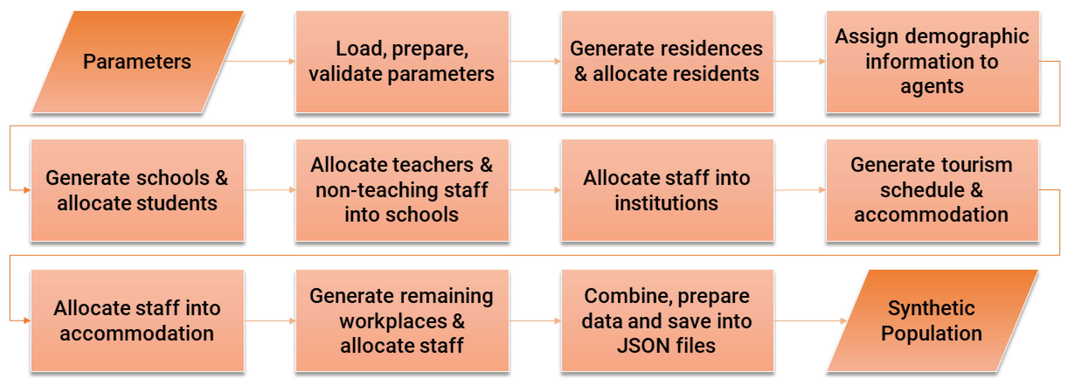
Figure 2.
High-Level Overview of the abm.
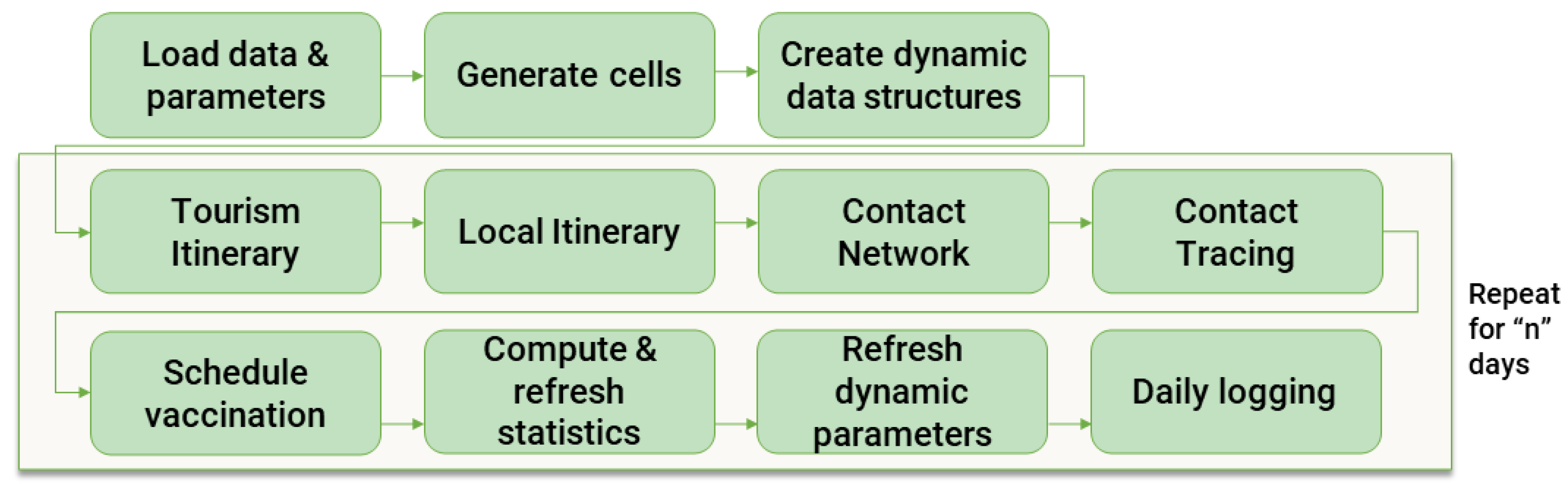
Figure 3.
A simple example of a potential contacts graph and direct contacts graph.
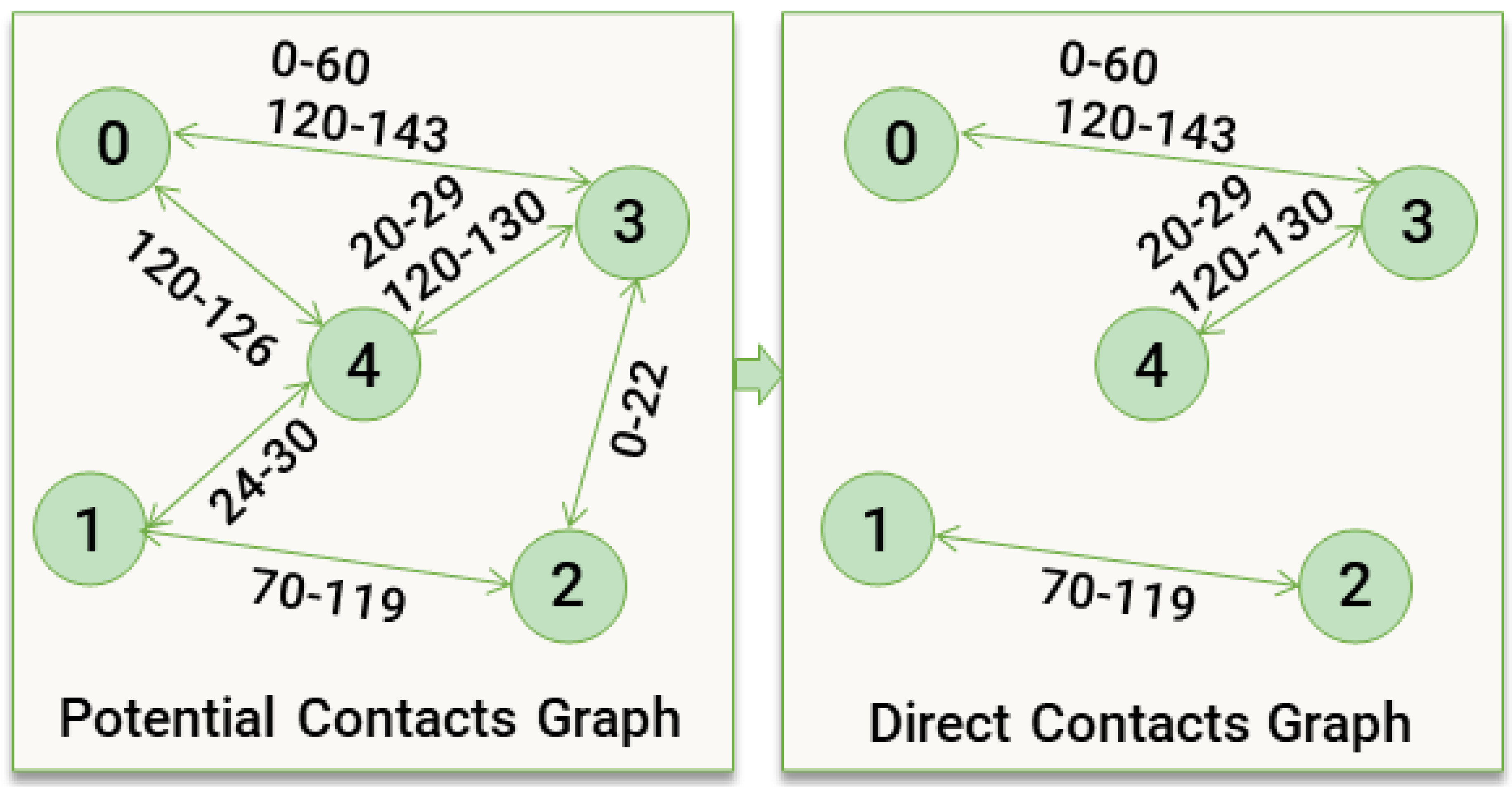
Figure 4.
Architecture diagram of mp.
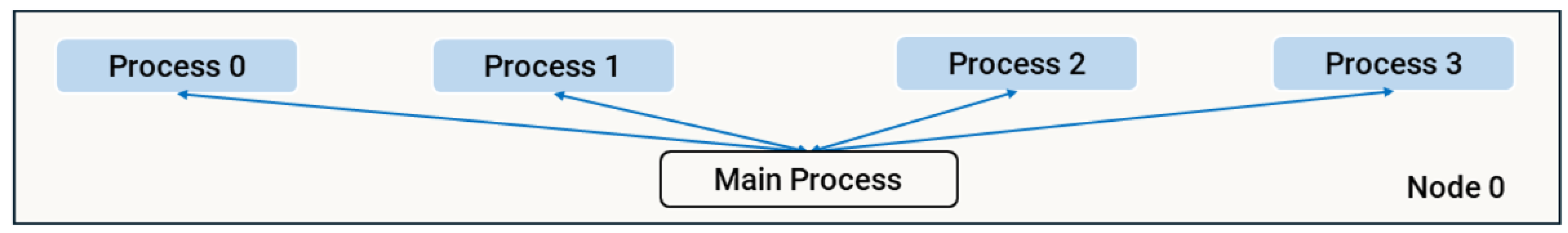
Figure 5.
Architecture diagram of d1.
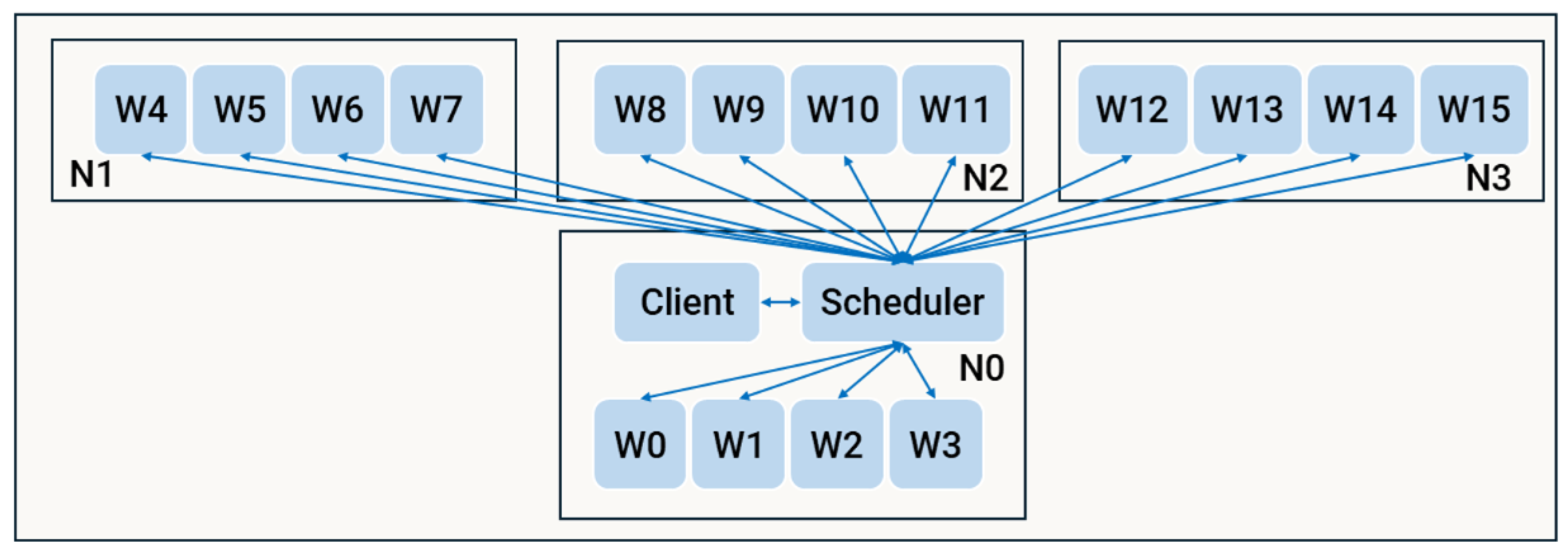
Figure 6.
Architecture diagram of d2.
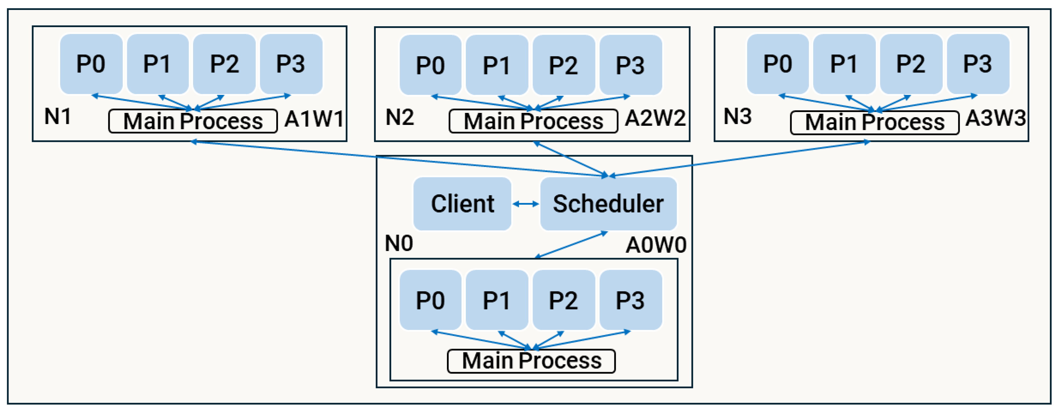
Figure 7.
Architecture diagram of d3.
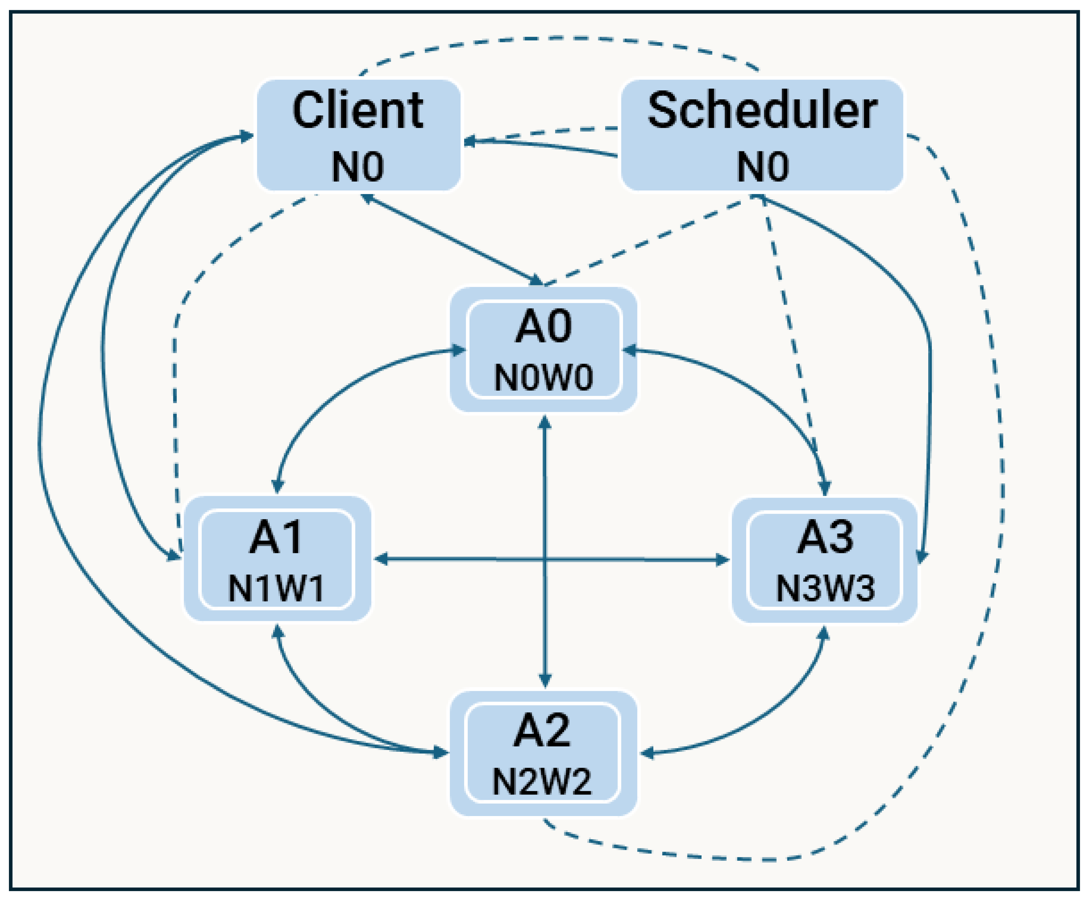
Figure 8.
A bar chart illustrating the age distribution and a comparison between actual and expected results.
Figure 8.
A bar chart illustrating the age distribution and a comparison between actual and expected results.

Figure 9.
Two bar charts: (a) depicting the enrollment status ratios for children aged 5-15; (b) detailing the age distribution of enrolled children aged 5-15 and a comparison of actual and expected outcomes
Figure 9.
Two bar charts: (a) depicting the enrollment status ratios for children aged 5-15; (b) detailing the age distribution of enrolled children aged 5-15 and a comparison of actual and expected outcomes
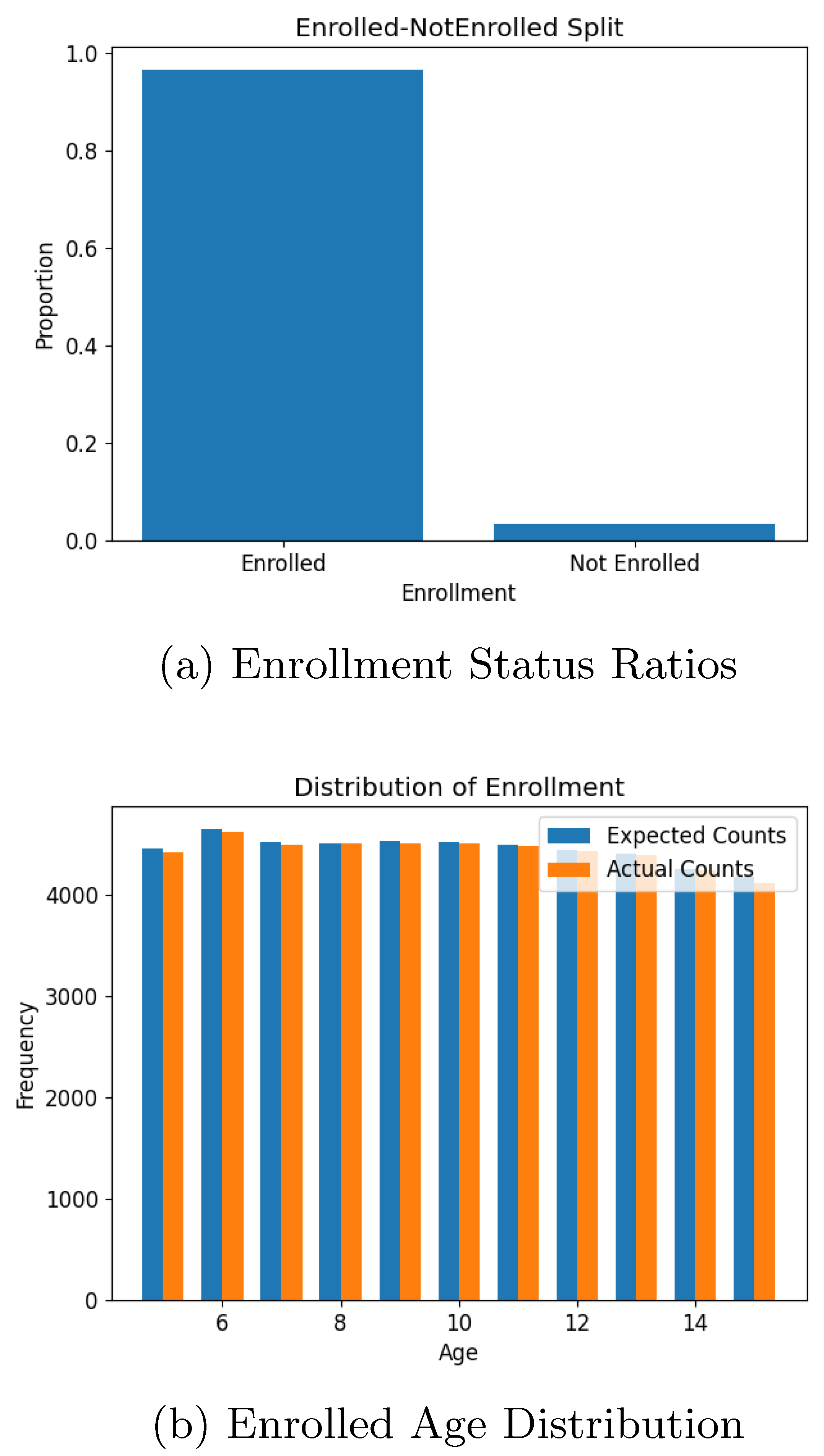
Figure 10.
Two bar charts: (a) presenting the employment status percentages among individuals aged 16-65; (b) showcasing the distribution across industries for employed agents, alongside a comparison between actual and expected figures
Figure 10.
Two bar charts: (a) presenting the employment status percentages among individuals aged 16-65; (b) showcasing the distribution across industries for employed agents, alongside a comparison between actual and expected figures
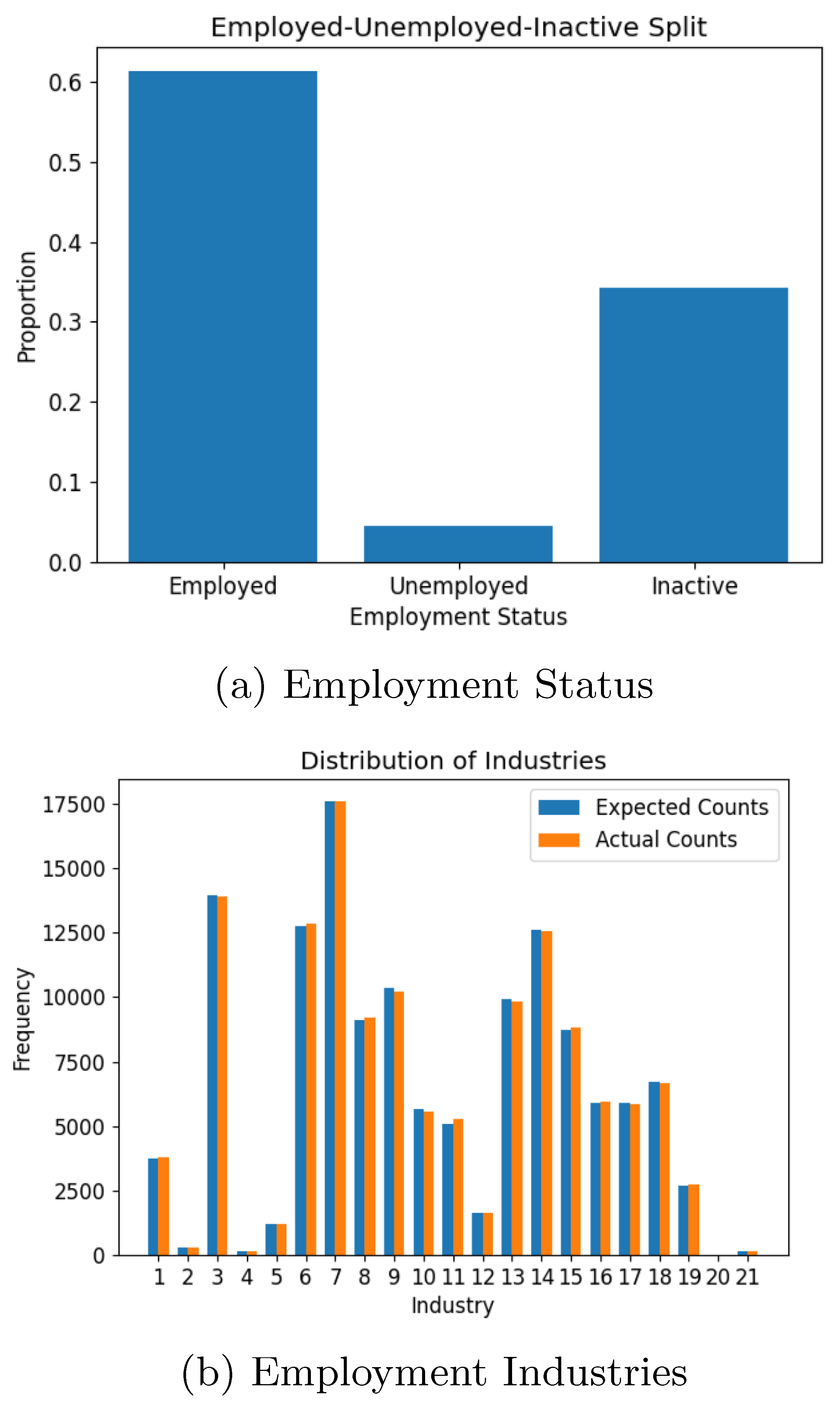
Figure 11.
Two bar charts: (a) outlining the age distribution (across age brackets) of incoming tourists and their comparison to expected outcomes; (b) illustrating the gender distribution among incoming tourists against expected results.
Figure 11.
Two bar charts: (a) outlining the age distribution (across age brackets) of incoming tourists and their comparison to expected outcomes; (b) illustrating the gender distribution among incoming tourists against expected results.
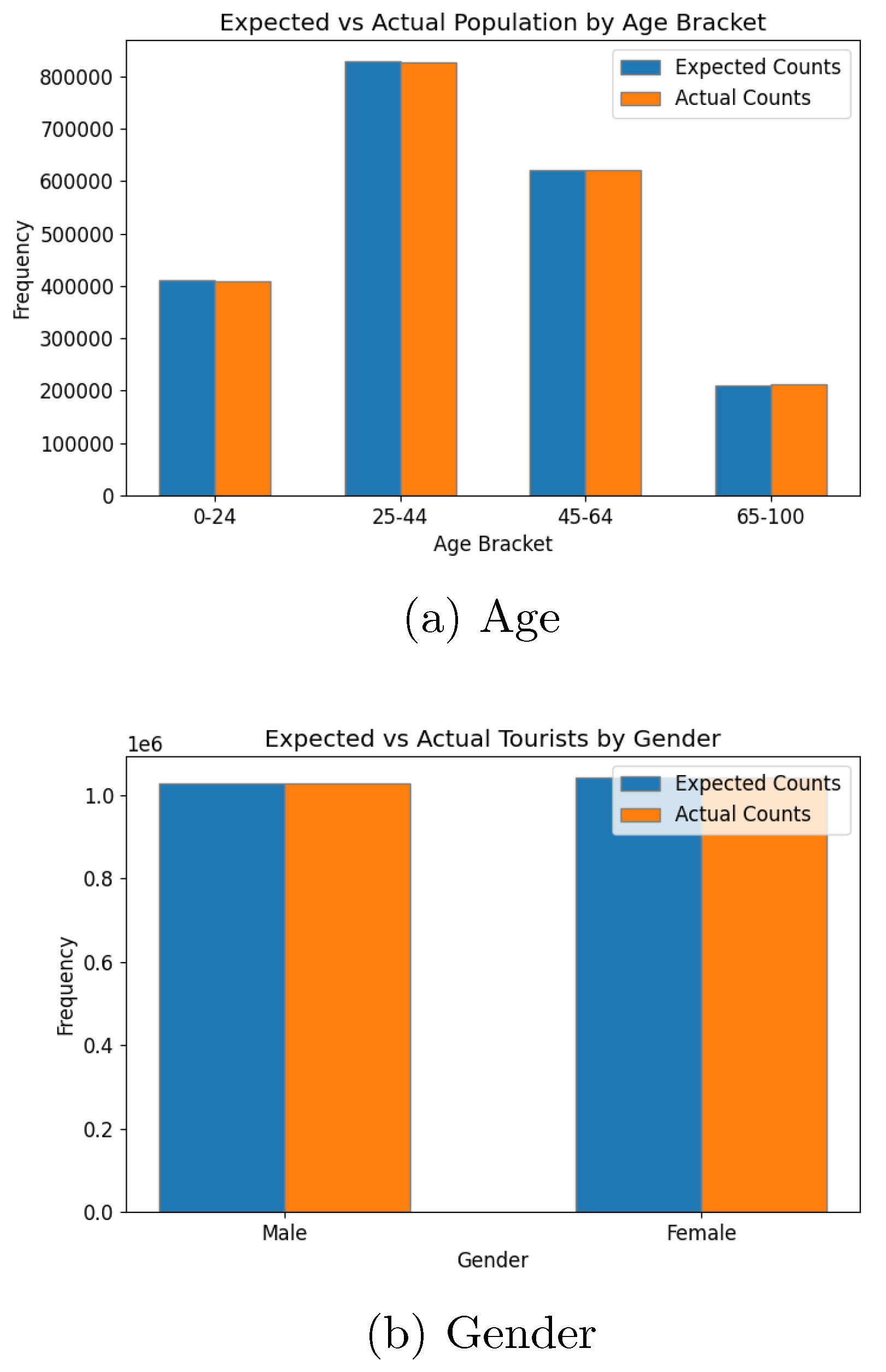
Figure 12.
Two bar charts: (a) illustrating the types of accommodations chosen by tourists, compared against expected outcomes; (b) detailing incoming tourist groups by travel purpose, comparing actual with expected results.
Figure 12.
Two bar charts: (a) illustrating the types of accommodations chosen by tourists, compared against expected outcomes; (b) detailing incoming tourist groups by travel purpose, comparing actual with expected results.

Figure 13.
Two bar charts: (a) showcasing the quarterly distribution of incoming tourist groups and their comparison to expected outcomes; (b) representing the travel duration distribution among tourists groups, compared to expected results.
Figure 13.
Two bar charts: (a) showcasing the quarterly distribution of incoming tourist groups and their comparison to expected outcomes; (b) representing the travel duration distribution among tourists groups, compared to expected results.
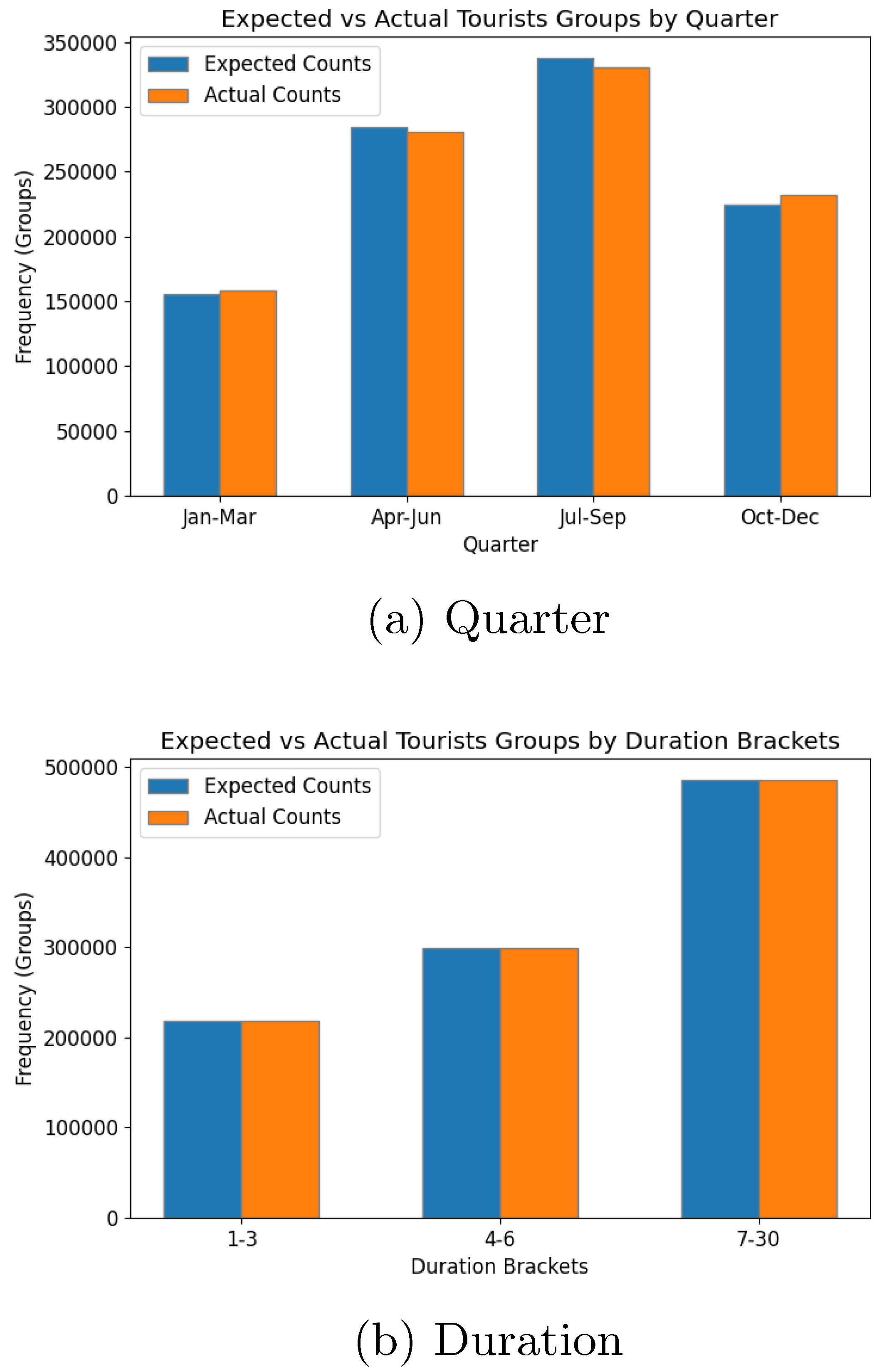
Figure 14.
A line chart showing the active cases over time, across the 3 main intervention levels
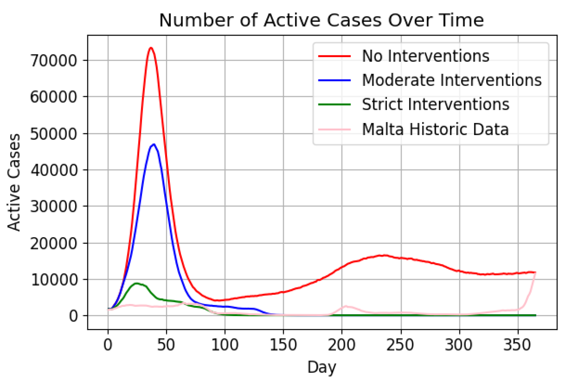
Figure 15.
2 line graphs comparing the 3 main intervention levels over time, showcasing: (a) the active recovery cases (b) the number of deaths.
Figure 15.
2 line graphs comparing the 3 main intervention levels over time, showcasing: (a) the active recovery cases (b) the number of deaths.
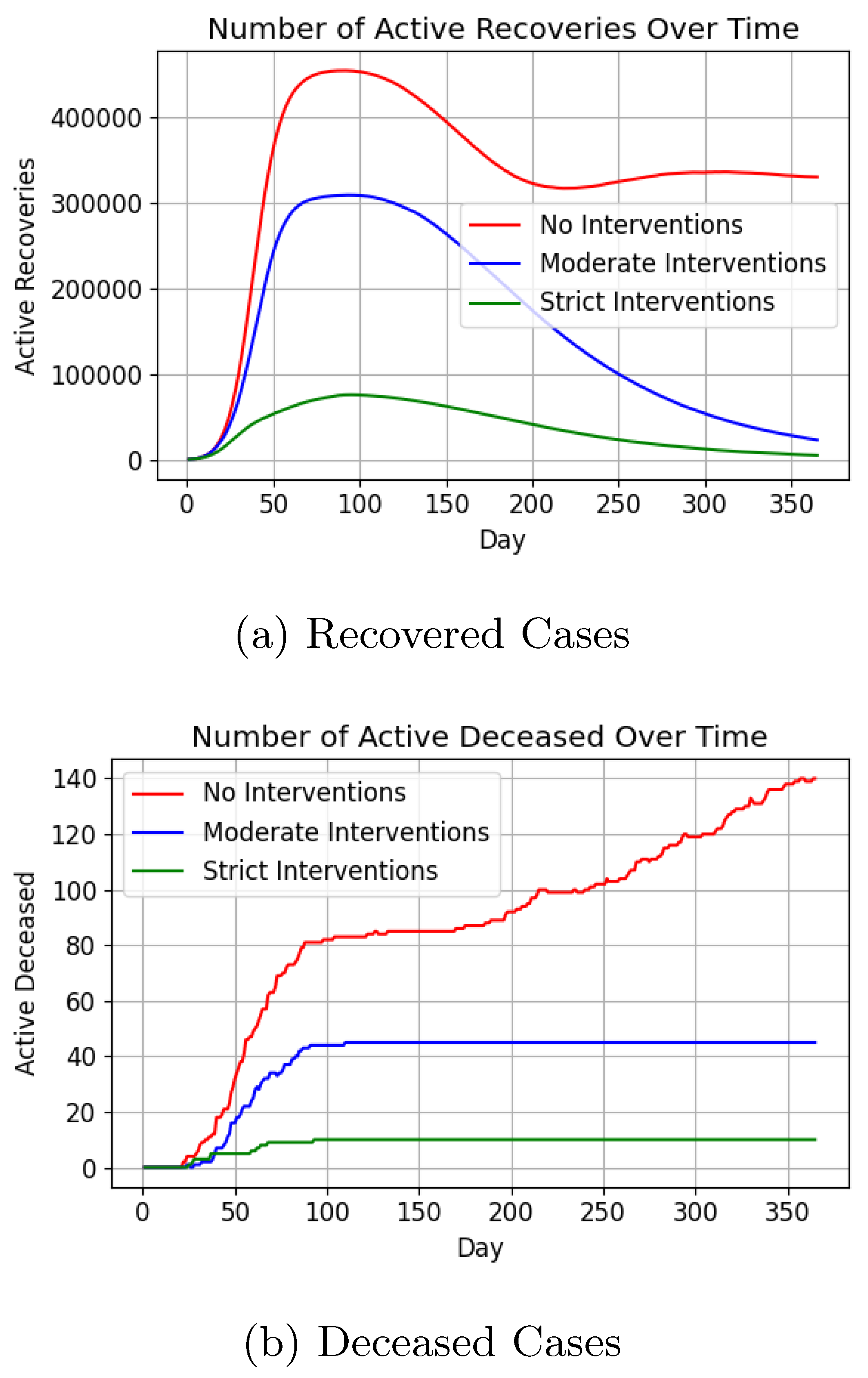
Figure 16.
2 line graphs comparing the 3 main intervention levels over time, showcasing: (a) new vaccinations (b) number of contact traced individuals.
Figure 16.
2 line graphs comparing the 3 main intervention levels over time, showcasing: (a) new vaccinations (b) number of contact traced individuals.
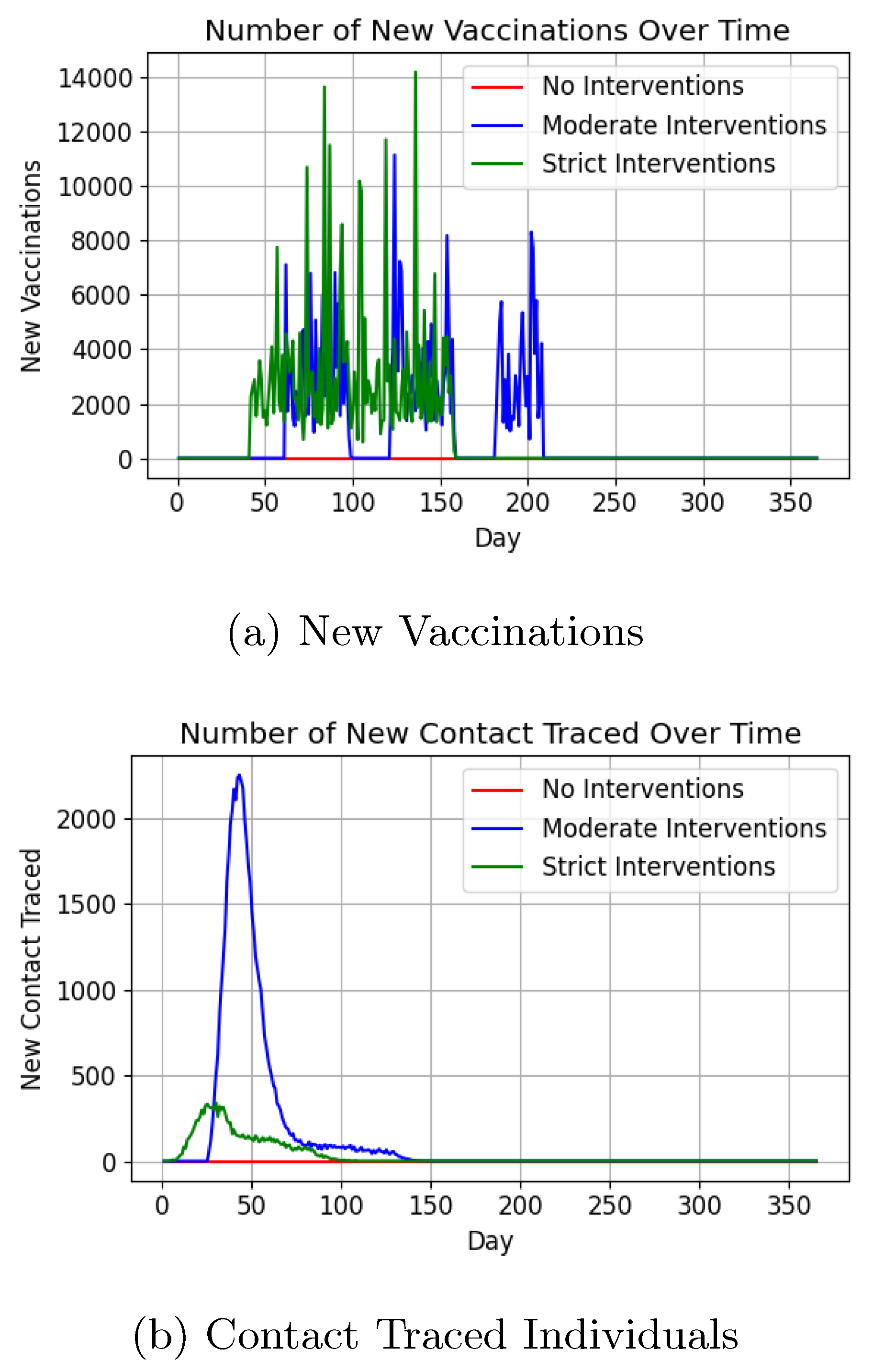
Figure 17.
A scatter plot demonstrating the effect of the different intervention levels on the average number of contacts.
Figure 17.
A scatter plot demonstrating the effect of the different intervention levels on the average number of contacts.
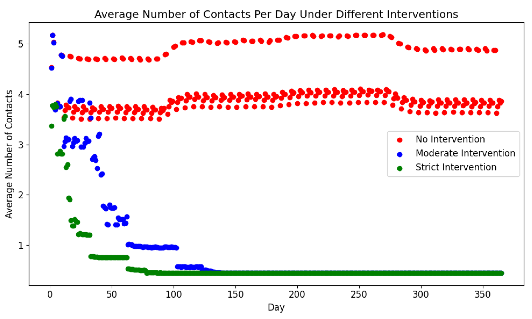
Figure 18.
A bar chart illustrating the frequency distribution across “never infected”, “infected once”, and “infected more than once” categories.
Figure 18.
A bar chart illustrating the frequency distribution across “never infected”, “infected once”, and “infected more than once” categories.
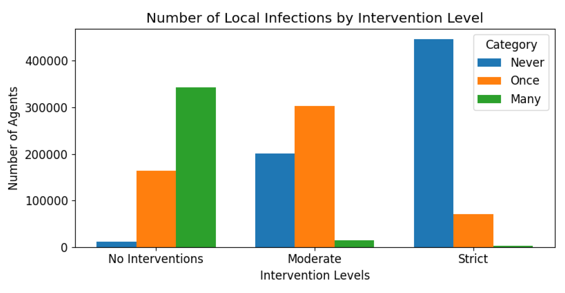
Figure 19.
Tourism and Travel Restrictions.
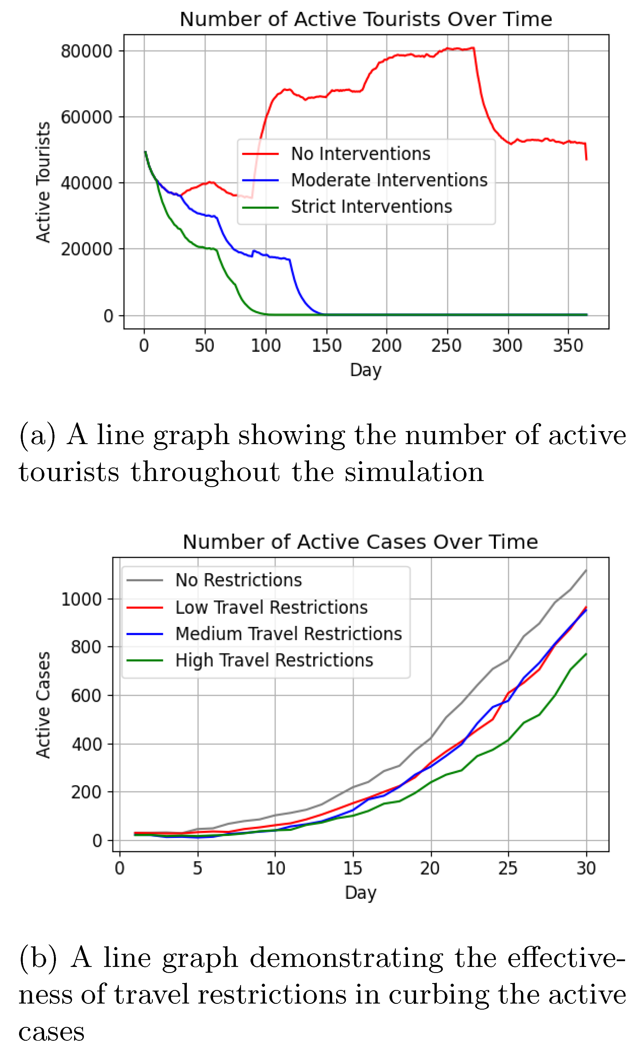
Figure 20.
Speed-up and efficiency plots based on a 7-day average.
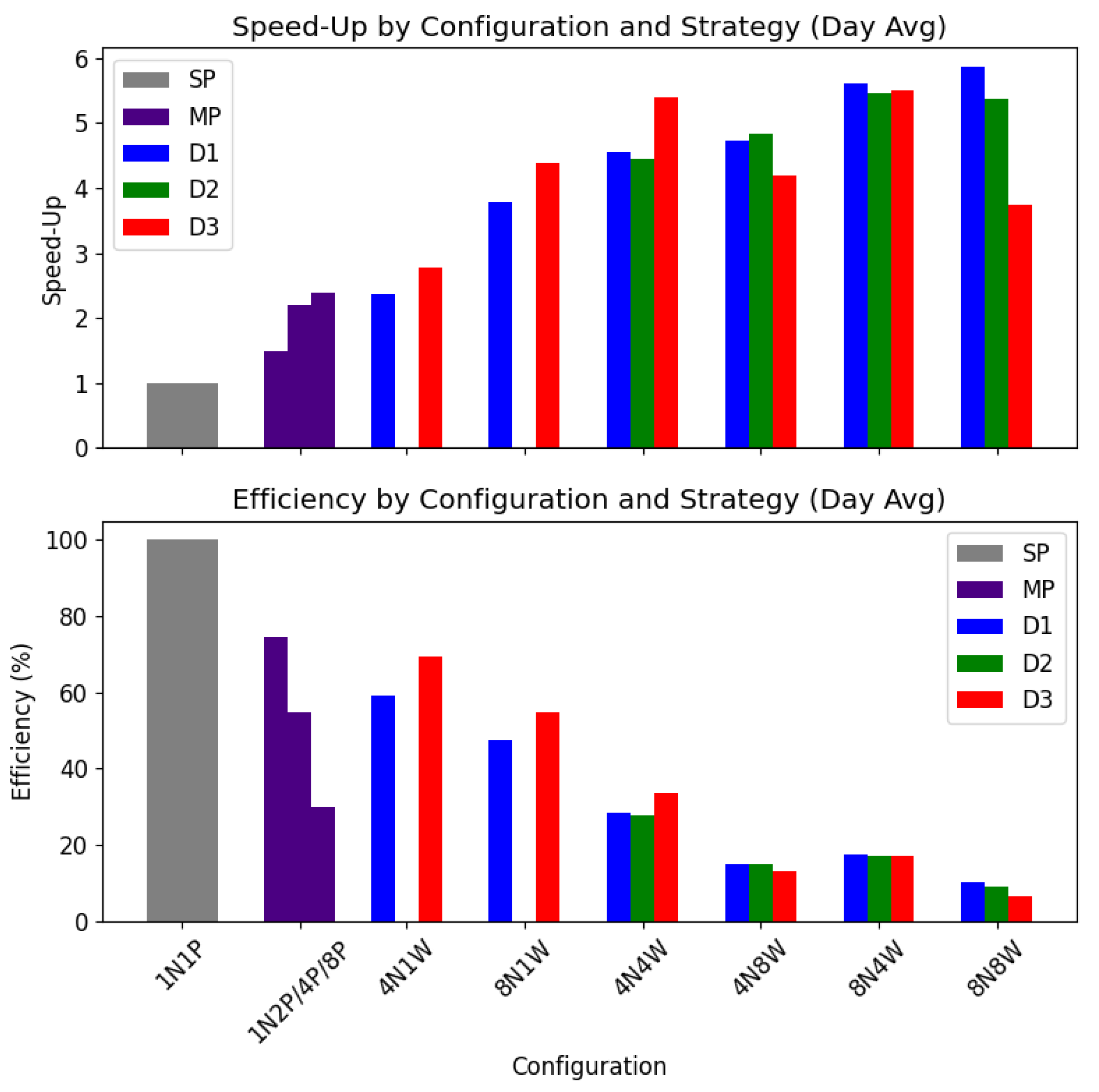
Figure 21.
Execution Time with increasing population sizes.
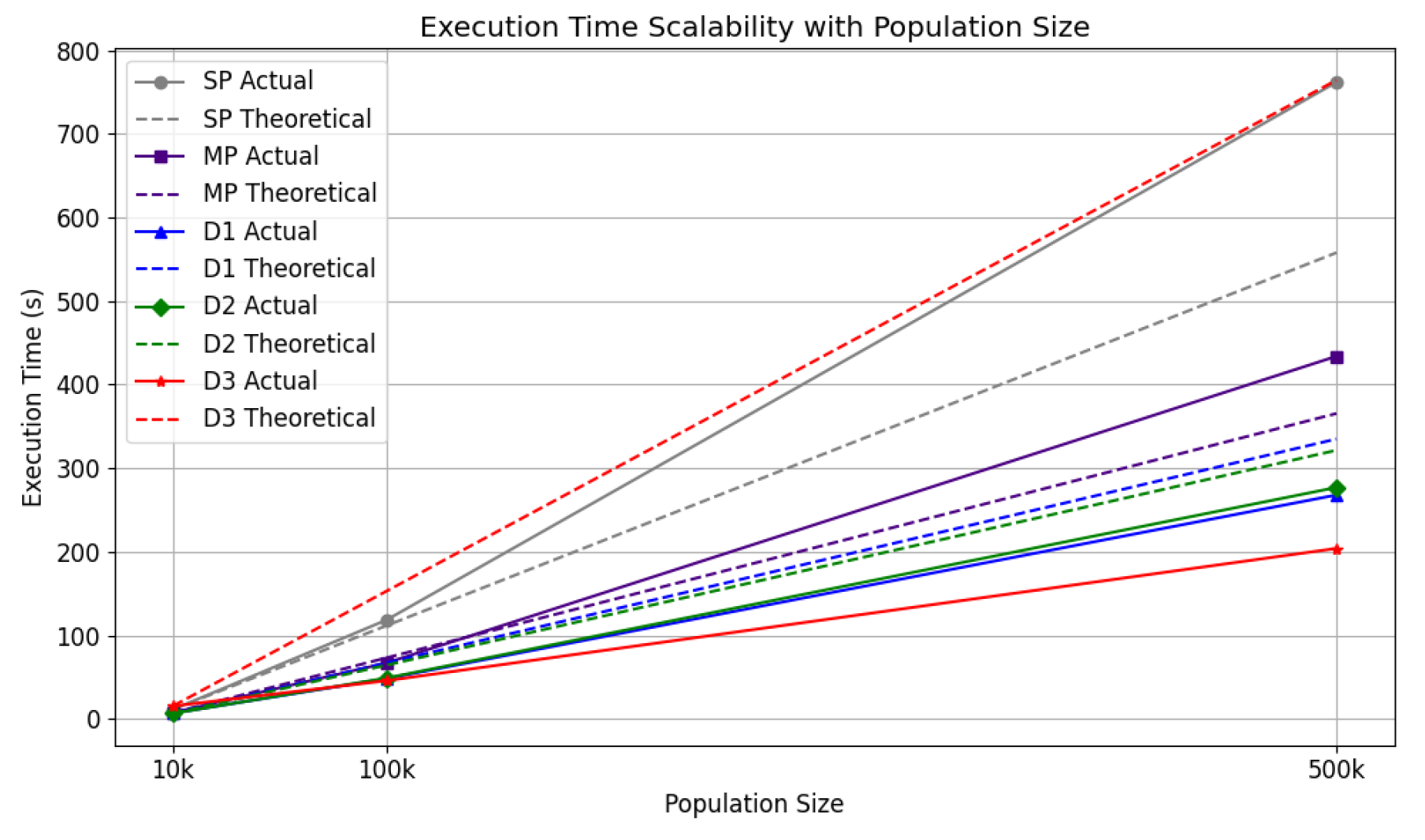
Figure 22.
Memory Usage with increasing population sizes.
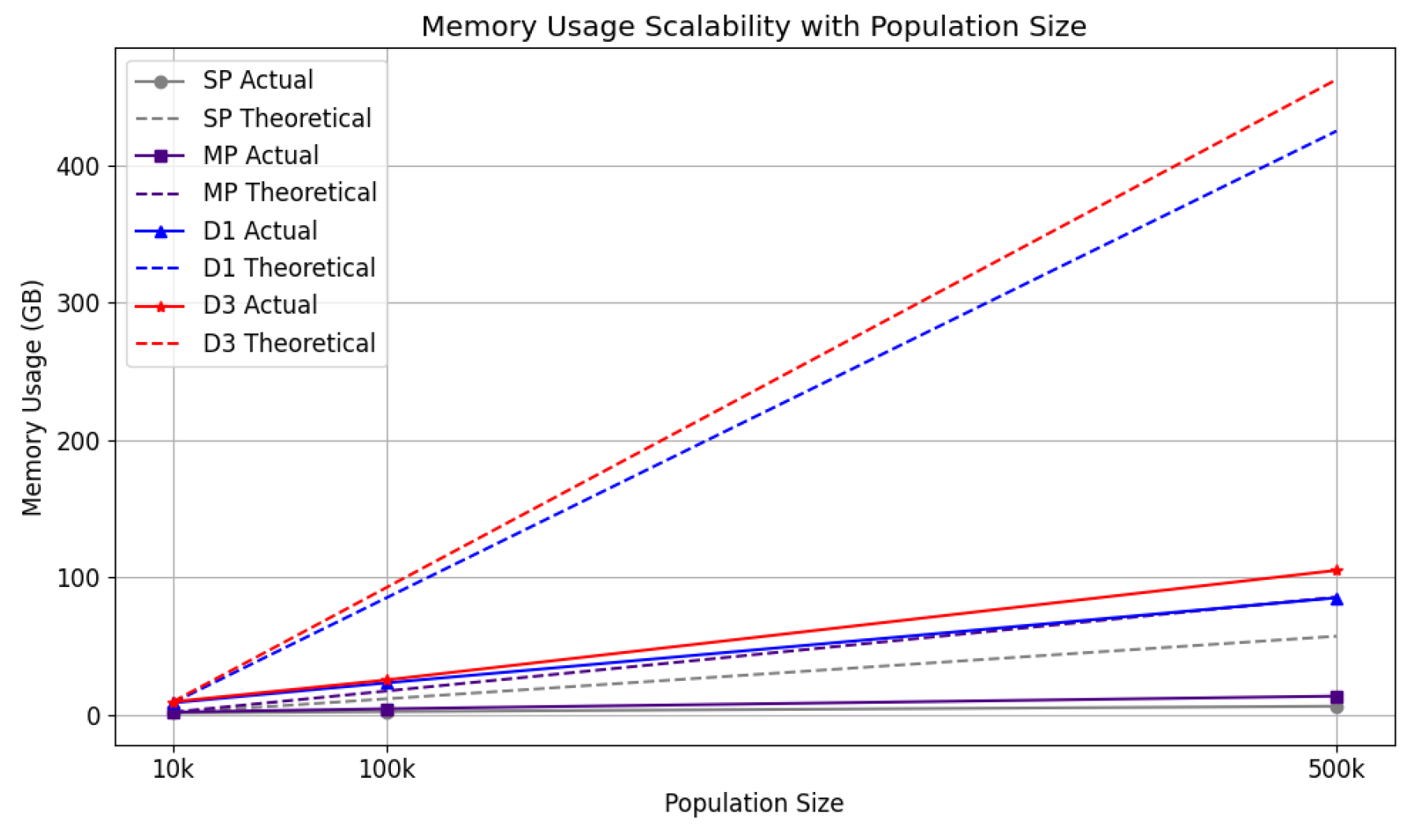

Table 1.
Execution Time Analysis (All except “T” and “ET” in seconds. “T” and “ET” in hours. Green for fastest time across the first 3 strategies; Blue where HPMP is fastest. T (Total), ET (Estimated Total without logging overhead), TO (Tourism), IT (Local Itinerary), CN (Contact Network), CT (Contact Tracing), VA (Vaccination)).
| Str. | T | ET | Init | Day | TO | IT | CN | CT | VA |
|---|---|---|---|---|---|---|---|---|---|
| MP | 45.25 | 32.58 | 108.76 | 446.01 | 48.26 | 167.44 | 197.61 | 27.93 | 0.02 |
| D1 | 32.50 | 22.56 | 298.68 | 319.78 | 41.68 | 134.62 | 103.74 | 34.77 | 0.02 |
| D2 | 34.89 | 26.07 | 183.14 | 343.64 | 42.78 | 138.22 | 122.00 | 35.59 | 0.02 |
| D3 | 19.91 | 19.50 | 478.56 | 195.06 | 1.95 | 73.46 | 79.60 | 27.70 | 0.14 |
| HPMP | 27.98 | 16.02 | 91.17 | 276.65 | 33.2 | 105.29 | 111.98 | 21.62 | 0.02 |
Disclaimer/Publisher’s Note: The statements, opinions and data contained in all publications are solely those of the individual author(s) and contributor(s) and not of MDPI and/or the editor(s). MDPI and/or the editor(s) disclaim responsibility for any injury to people or property resulting from any ideas, methods, instructions or products referred to in the content. |
© 2025 by the authors. Licensee MDPI, Basel, Switzerland. This article is an open access article distributed under the terms and conditions of the Creative Commons Attribution (CC BY) license (http://creativecommons.org/licenses/by/4.0/).
Copyright: This open access article is published under a Creative Commons CC BY 4.0 license, which permit the free download, distribution, and reuse, provided that the author and preprint are cited in any reuse.


