Development of Economic and Mathematical Tools for Analyzing and Evaluating the Value of Life Based on Willingness to Pay for Mortality Risk Reduction (Using Air Pollution as an Example)

Polina Poplavko; Artur Nagapetyan

doi:10.20944/preprints202502.1023.v1

Submitted:

13 February 2025

Posted:

13 February 2025

You are already at the latest version

Abstract

This study proposes an approach to assessing the Value of Statistical Life (VSL) based on the contingent valuation of willingness to pay for reducing the risk of mortality caused by air pollution from port activities in port city residents. The research involves data collection through a survey utilizing a double dichotomous choice method. The proposed approach differs from existing ones by introducing a new way of estimating the marginal willingness to pay for each additional unit of risk reduction. These estimates are obtained by approximating the corresponding dependency using an elementary function based on five available coordinate points. These coordinates reflect the marginal willingness to pay for each additional unit of risk reduction, as derived from five different risk reduction scenarios presented in the survey. To more accurately assess the declining willingness to pay, an adjustment for cognitive biases is suggested by incorporating questions that evaluate respondents' competency in working with percentage points. It is assumed that the proposed approach will help mitigate the well-known issue in the literature regarding the dependence of VSL estimates on survey design, particularly the level of risk reduction considered. This, in turn, will reduce the manipulability of such studies and significantly enhance trust in their results.

Keywords:

Value of a Statistical Life (VSL)

;

Stated preference method

;

willingness to pay (WTP) sensitivity

;

contingent valuation method

;

air pollution

;

Scaling problem (disproportionality)

;

Scale Sensitivity Test

Subject:

Business, Economics and Management - Econometrics and Statistics

Introduction

Environmental pollution is one of the most significant health risk factors. According to the World Health Organization, air pollution alone causes seven million deaths annually worldwide. Reducing mortality associated with air pollution requires substantial financial investments. However, the effective allocation of resources in this area is only possible with an understanding of how much society is willing to invest in preserving each additional life, known as the Value of a Statistical Life or VSL, or in preventing a fatality, referred to as the Value of Prevented Fatality.

The stated preferences method is used to assess willingness to pay. This approach allows us to determine how individuals value life preservation through hypothetical scenarios and questions regarding their readiness to incur financial costs to reduce risks. Although the revealed preferences method, which is based on actual behavior, is widely used, it is the stated preferences method that provides the opportunity to study willingness to pay for goods that are not observable in the market, such as clean air and reduced mortality risk. In recent decades, interest in this approach has grown significantly, confirming its relevance for evaluating the economic value of reducing environmental risks.

This research develops a methodology aimed at improving the accuracy of life valuation estimates by addressing the issue of "manipulability" in the valuation of life. To obtain life value estimates through the contingent valuation method with willingness to pay (WTP), an original survey was developed, focusing on the impact of air pollution on the health of residents in port cities. This goal is achieved by providing a more accurate assessment of willingness to pay, accounting for potential cognitive biases, by considering five different levels of mortality risk reduction (five groups) and further segmenting respondents into groups with higher and lower levels of cognitive bias.

Research question: How can the variability in estimates of the value of statistical life be reduced by refining the questionnaire design methodology?

Research hypotheses are as follows:

Increasing the magnitude of the proposed risk reduction will lead to respondents being, on average, willing to pay a progressively lower amount for each additional percentage point of risk reduction.
For subgroups with lower levels of cognitive bias, the effect of disproportionate sensitivity in willingness to pay for each additional percentage point reduction in mortality risk will be less pronounced compared to subgroups with higher levels of cognitive bias. Estimating the function that characterizes the declining willingness to pay, adjusted for cognitive biases, will yield more accurate estimates of the value of life.
Estimates of the impact of basic socioeconomic and demographic characteristics on willingness to pay (e.g., gender, age, education, income, marital status) will be biased in models that do not employ quasi-experimental methods for causal inference, particularly the instrumental variable method.

The research problem is that changes in the magnitude of risk reduction may lead to disproportionate changes in willingness-to-pay estimates, all else being equal. This results in a significant dependence of value-of-life estimates on the specific features of the research design and study structure.

Literature Review

The importance of proportionality as a crucial and essential component of value-of-life estimates based on contingent valuation can be explained using the basic concept proposed by Hammitt, J. K. in 2000 [Hammitt, J. K., Liu, J.-T., & KLin, W.-C., 2000].

V S L = \frac{d w}{d p} = \frac{u_{a} (w) - u_{d} (w)}{(1 - p) {u'}_{a} (w) + p {u'}_{d} (w)}

(1)

Where

u_{a}

(w) represents the utility of wealth if an individual survives until the end of the period, and

u_{d}

(w) represents the utility of wealth if an individual dies (for example, the utility derived from an inheritance), the VSL—defined as the marginal rate of substitution between income and the probability of surviving for one year (with the income proxy being the amount an individual is willing to pay to reduce health risk)—takes the following form:

VSL = ΔWTP/ Δp

(2)

The proportional change is described by the following formula, according to which the ratio of the higher willingness to pay to the lower willingness to pay corresponds to the ratio of the larger risk reduction to the smaller risk reduction:

\frac{{W T P}_{l a r g e}}{{W T P}_{s m a l l}} = \frac{{Δ p}_{l a r g e}}{{Δ p}_{s m a l l}}

(3)

In the case of disproportionate change, a problem arises with the manipulation of the mortality risk reduction indicator, as the value-of-life estimate will then fall within a range determined by the magnitude of the mortality risk specified in the willingness-to-pay question. Disproportionality occurs for several reasons, the primary ones being cognitive biases stemming from a misunderstanding of probabilistic changes or insensitivity to the presented scenario, and a decreasing marginal utility of risk reduction. However, when the marginal utility of mortality risk reduction diminishes, the resulting estimates do not conform to expected utility theory. At the same time, a misunderstanding of probabilistic changes leads to an underestimation or overestimation of the willingness-to-pay estimates, thereby compromising the reliability of the value of statistical life assessments.

A large body of empirical and review evidence suggests that there is a problem of disproportionality in willingness-to-pay estimates relative to the magnitude of mortality risk reduction. For example, between 1980 and 1998, as Hammitt J. K. and Graham J. D. reported in a review [Hammitt J. K., Graham J. D.,1999] of stated preferences, in 25 studies that numerically estimated the magnitude of the reduction in mortality risk, the estimates were disproportionate. Even the introduction in 1993 by a group of experts from the National Oceanic and Atmospheric Administration (NOAA) of mandatory requirements for external tests to verify disproportionality did not solve this problem [Arrow K. et al., 1993]. As shown by Krupnik A. in the 2007 review: out of 28 studies conducted, 20 applied tests that showed disproportionality of estimates.

To illustrate the problem, consider the following example that demonstrates the instability of value-of-statistical-life estimates due to variability in the levels of mortality risk reduction. For instance, if the willingness to pay for a 0.025 percentage point reduction in mortality risk is 1,000 rubles, then the overall estimate of the value of prevented fatalities would be 4 million rubles:

V S L = 1000 * \frac{100}{0,025} = 4 000 000 .

According to the theory, if a 0.05 percentage point reduction in mortality risk is specified instead of 0.025 percentage points, respondents should be willing to pay twice as much—i.e., 2000 rubles. In that case, the value-of-life estimate will remain at the same level:

V S L = 2000 * \frac{100}{0,05} = 4 000 000

If, however, for a 0.05 percentage point reduction the respondent is willing to pay not 2000 but a less proportional amount—for example, 1500—then the value-of-life can be estimated at 3 million rubles:

V S L = 1500 * \frac{100}{0,05} = 3 000 000

.

In the end, the value-of-life estimates fall within a certain range—for example, from 3 to 4 million rubles—which leads to a lack of confidence in the obtained values. To address this problem, the authors propose several approaches. The majority of studies focus on reducing cognitive biases through various methods. For instance, in the article by Corso, Hammitt, and Graham (2001), visual tools such as a logarithmic scale, a linear scale, an array of points, and even no visualization are used to convey the baseline risk of death. According to model evaluations, WTP is more sensitive to risk reduction when an array of points or a logarithmic scale is used. Visual tools can be employed not only to improve the understanding of probabilistic changes in mortality risk reduction but also to collect data on perceived mortality risk, as demonstrated in the work by Leiter and Pruckner (2009). A scale similar to Corso’s logarithmic scale was used as a variable, where respondents assessed the average risk of death from an avalanche by indicating their estimate on a scale from 0 to 130 mm.

Another tool for addressing the issue of disproportion is the use of questions aimed at understanding probabilistic changes. This approach is frequently employed in research, yet it does not always yield positive results. For example, Hammitt, J. K. and Graham, J. D. used a question involving a comparative analysis of mortality indicators to compare the proportionality of WTP responses between respondents who provided correct answers and those in a comparison group. However, this instrument did not prove effective.

Leiter A. M. employed questions designed to assess the understanding of probabilistic changes within a training framework. A distinctive feature of these questions was that an explanation was provided after each question, except for the last one. Respondents who answered all questions incorrectly were excluded from the sample. It was found that excluding these non-trained respondents from the models increased the willingness-to-pay estimates for mortality risk reduction, thereby enhancing the proportionality of the results.

Alolayan, Evans, and Hammitt (2017) [Alolayan M. A., Evans J. S., Hammitt J. K., 2017] reached similar conclusions and proposed an "innovative consistency test" based on respondent weighting to assess the proportionality of WTP estimates for mortality risk reduction. Their survey incorporated training questions, comprehension tests, scenario rejection items, and visual aids, with respondents randomly receiving high or low risk reduction options. Only responses with strictly positive and nearly proportional WTP were used in calculating the VSL, increasing estimates from $10 million to $18–32 million. Although the authors consider the test useful for filtering irrelevant data, they acknowledge it does not fully ensure result validity. An alternative approach using latent class models [Hammitt & Herrera-Araujo, 2018] also produced inflated VSL estimates.

Methods and Data

The double-bounded dichotomous choice model (DBCM) or interval data was used to collect data on willingness to pay to reduce the risk of death. The statistical power of this model was demonstrated in the work of Hanemann et al [Hanemann, M., Loomis, J. & Kanninen, B. 1991].

Based on information about respondents (socio-economic, demographic, behavioural characteristics), the willingness-to-pay estimate is further modelled using the following linear function [Lopez-Feldman A., 2012]:

{W T P}_{i} (z_{i}, u_{i}) = z_{i} β + u_{i}

(4)

z_i - is a vector of explanatory variables (characteristics of the respondent), β is a vector of parameters and u_i is a random error.

To estimate the coefficients of this model, it is necessary to form a logarithmic maximum likelihood function, the maximization of which will allow us to determine such values of the coefficients of model (1) at which the probability of obtaining the observed data collected in the survey process will be the highest.

Study Design

To address the research hypotheses, data will be collected using a custom questionnaire presented after the study design description (Appendix A). In developing the questionnaire, best practices in designing surveys for contingent valuation of willingness to pay [Sajise A. J. et al., 2021] and for estimating the value of statistical life based on willingness to pay for reducing the risk of death [Hammitt J. K., Graham J. D., 1999] were employed. The sections were organized to gradually introduce respondents to the context of the problem and reveal their risk perceptions related to air pollution. The primary objective is to determine the extent to which people are willing to pay to reduce the harmful effects of port activities on the health of port city residents. An analysis of studies on contingent valuation for reducing the risk of death from air pollution reveals insufficient examination of sensitivity to the proposed scenario associated with the experience of living near pollution sources. To address this, respondents were divided into two groups based on their potential health risk exposure: those residing in port cities and those not residing in port cities. This division allows for an assessment of how experience influences willingness-to-pay estimates.

The relevance of the chosen topic is underscored by the fact that in 2024, César Ducruet and co-authors, analyzing data from 5,000 ports in OECD countries for the period from 2001 to 2018, demonstrated that ports are one of the significant sources of air pollution. For example, in densely populated port cities, the concentration of particulate matter (PM2.5) and NOx can be 30–40% higher, which increases the incidence of respiratory and cardiovascular diseases [Ducruet C. et al., 2024].

Statistically and economically significant differences in willingness-to-pay estimates for the corresponding levels of mortality risk reduction will allow us to test the first hypothesis. The key distinction of the proposed approach from existing methods lies in obtaining estimates of marginal willingness to pay for each additional unit of risk reduction, rather than scaling the willingness to pay for a single risk level to 100 percentage points. These estimates are derived by approximating the relevant relationship using an elementary function based on five available coordinates that characterize the marginal willingness to pay for each additional unit of risk reduction. Although constructing a function based on five points may have its limitations, this approach will enable a deeper understanding of the true nature of WTP.

Mortality risk reduction levels are exogenously and randomly assigned to different groups of respondents (Table 1), which helps avoid the self-selection problem. The test proposed by the authors is an external scope test, which, according to Krupnick (2007), is more informative and less susceptible to the anchoring effect compared to internal scope tests (Yeung, Smith, & McGhee, 2003). To test hypothesis 2, the questionnaire includes control questions designed to assess respondents' ability to solve problems involving probabilistic changes.

Dividing respondents into two subgroups based on the degree of cognitive biases will allow us to test Hypothesis 2 and determine whether there are statistically and economically significant differences between the corresponding indicators. Confirming this hypothesis will require using the five coordinates obtained in the study for the subgroup with a lower level of cognitive biases to estimate the marginal willingness to pay for each additional unit of risk reduction. To achieve this, the questionnaire includes control questions (Part 2) aimed at assessing respondents’ ability to solve problems involving probabilistic changes. This approach will help avoid a potential underestimation of the final value-of-life estimate.

Table 2 presents the structure of the questionnaire, with a brief explanation of the purpose of including this item in the design. According to Table 2, part 5 of the questionnaire presents socio-demographic characteristics. This item is necessary not only to collect information about important characteristics of the respondent, but also to understand their lifestyle. The authors identify the religious affiliation, activities of the respondent. As Leiter A. writes, in the study of disproportionality it is the consideration of behavioral characteristics that helps to obtain more proportional estimates of willingness to pay, as well as to explain the nature of WTP [Leiter A. M., Pruckner G. J., 2009].

These levels of mortality risk reduction, combined with tools for segmenting respondents based on the degree of cognitive bias, could help disentangle the effects of diminishing marginal utility of mortality risk reduction from cognitive biases. A third factor that could help address disproportionality arising from potential insensitivity to the proposed risk reduction scenario is the use of questions related to lifestyle and worldview characteristics. These include questions from Part 4 of the survey ("Health"), which focus on lifestyle assessment, including self-evaluation of health, attitudes toward health, chronic diseases, and harmful habits (such as smoking and alcohol consumption).

To test the third hypothesis, we plan to compare the coefficients representing the influence of the corresponding factors (Parts 4 and 5) on willingness-to-pay estimates for reducing mortality risk in both the baseline models and those employing the instrumental variable method. The necessary data for constructing the instrumental variables will be collected through additional questions—for example, asking about the mother's level of education to assess the impact of the respondent's education on their income and overall educational attainment.

Despite a substantial body of empirical and theoretical literature, the issue of disproportionate willingness-to-pay (WTP) estimates for reducing mortality risk remains insufficiently explored and requires further in-depth analysis. The implementation of this study will allow us to determine the presence of statistically and economically significant differences in WTP estimates and, based on these findings, understand how to reduce the variability of value-of-life estimates through improvements in questionnaire design methodology. Moreover, this research will help identify the factors influencing WTP for reducing the risk of death from air pollution and develop approaches to eliminate disproportion in these estimates, which is crucial for further scientific inquiry. The study’s results may be used to inform well-founded environmental policies that account for regional differences, as well as in other contexts.

Conflicts of Interest

The authors declare no conflicts of interest.

Appendix A

The questionnaire

(The original language of the study is Russian. The questionnaire is presented in English)

We ask you to take part in our survey on the assessment of the situation related to air pollution in the regions of the Russian Federation and measures to reduce harmful effects on the health of their residents.

Your answers are confidential and will be used only in a generalized form. Participation is voluntary and anonymous. The survey takes about 20 minutes to complete. We thank you for your participation and support of our study!

If you have any questions or comments, you can contact us by mail.

If you are 18 years of age or older and would like to continue to participate in this survey, please select the appropriate option:

☐ Yes, I am 18 years old and agree(s) to participate in the survey
☐ No, I do not agree to take the survey or I am under 18 years of age.

Part 1. Experience of living in a port city and quality of life

1. Select the statement that describes your experience of living in a port city.

☐ I have never lived in a seaport city/area
☐ I have lived in a port city/area
☐ I live in a port city/area
☐ I visit port cities (holiday, business trip)

2. Have your close relatives/friends lived/are living in the port city/area?

☐ Yes, they do now
☐ Yes, used to live in the past
☐ No

Quality of life

2.1 Estimate approximately the distance from the port to your last place of residence (in the port city)?

☐ Less than 5 km
☐ From 5 to 10 km
☐ 10 to 50 km
☐ 50 to 100 km
☐ More than 100

2.1 Estimate approximately the distance from the port to your place of residence?

☐ Less than 5 km
☐ 5 to 10 km
☐ 10 to 50 km
☐ 50 to 100 km
☐ More than 100

3. Considering all aspects of life, how satisfied are you with your life in general at present? Give your answer on a scale from 1 to 5, where ‘1’ means ‘absolutely NOT satisfied’ and ‘5’ means ‘completely satisfied’.

1

2

3

4

5

4. How many years do you think the average person's life expectancy could be reduced by, solely because they live in an area with dirty air?

☐ 1-3 years
☐ 3-5 years
☐ 6 - 10 years
☐ 11 - 15 years
☐ More than 15 years

5. Do you think air quality affects your health?

In front of you is a scale from 1 to 5, where 1 means ‘Absolutely No Effect’ and 5 means ‘Strongly Affects’

1

2

3

4

5

6. How would you rate the air quality in your place of residence based on the following characteristics (e.g., visibility of smoke, presence of dust, unpleasant smells (cinders, car exhaust, etc.)?

In front of you is a scale from 1 to 5, where 1 means ‘very poor air quality’ and 5 means ‘very good air quality’.

1

2

3

4

5

Part 2.

7. If, all other things being equal, in the FIRST region of Russia the probability of contracting a respiratory tract infection is 12 per 1000 people and in the SECOND region 8 per 1000 people, in which region is the risk of infection HIGHER?

In the FIRST region
In the second region
The probabilities are the same

8. What is the risk of death for an average motorist in Russia who always wears a seatbelt compared to someone who never wears a seatbelt, if it is known that seatbelt use reduces the risk of mortality by 40-50%, and the mortality rate among unbelted people is 2 deaths per 100,000 people according to Rosstat?

10 cases per 1,000,000 people
10 cases per 100,000 people

9. According to the data for 2024 in Russia, 250 per 100,000 people die of cancer annually’. If, due to the introduction of new technologies to combat cancer, this rate is reduced by 5 per 10,000 people, what will be the probability of death from cancer?

2 deaths per 1,000 people
200 deaths per 100,000 people
All options are correct

Part 3. Description of the initiative and assessment of willingness to pay.

All information is based on reliable sources (WHO data, Rosstat, scientific articles)

1.How does air pollution affect health?

Approximately 7 million people worldwide die each year from air pollution-related causes.

Air pollution leads to increased morbidity and premature death from:

-: cardiovascular diseases (coronary heart disease, stroke);
-: respiratory diseases (bronchitis, COPD, pneumonia);
-: oncological diseases (lung cancer).

2. What is the mechanism of health effects of suspended particulate matter?

Air pollution by suspended solids (dust, PM10, PM2.5) causes the most severe health effects.

-

PM10 particles penetrate into the lungs and, once deposited, cause inflammation, irritation and damage to the mucous membranes of the respiratory tract.

-

PM2.5 particles are smaller and more dangerous particles. They penetrate through lung tissue into the bloodstream, leading to:

○: to chronic vascular inflammation, which raises blood pressure and, increases the risk of stroke.
○: long-term inflammation of the lungs and other organs creates conditions for the development of cancerous changes.

3. How do Particles affect population mortality?

Epidemiological data show that for every 10 µg/m3 increase in PM2.5 particle concentrations, there is an increase:

-: total mortality by 4%,
-: cardiopulmonary mortality by 6%,
-: lung cancer mortality by 8%,
-: mortality from respiratory diseases by 0.58%
-: hospitalization rate by 8%.

4. What are the mortality rates from air pollution-related diseases in the Russian Federation?

According to the data of 2023 in the Russian Federation:

-

1 place in the mortality structure is occupied by: diseases of the circulatory system (556.7 per 100 thousand population), of which:

○: ischemic heart disease - 297.9 per 100 thousand people
○: strokes - 75.2 per 100 thousand people

-

2nd place: neoplasms (197 per 100 thousand people), including:

○: Malignant neoplasms of trachea, bronchi, lung (17.6%) - the most common oncological disease.

-

3rd place - respiratory diseases (53 per 100 thousand people).

5. How do ports affect air pollution?

Seaports are major logistics hubs where sources of air pollution include:

-: ships;
-: coal terminals;
-: railway and road transport;
-: transported cargo.

The most significant health impact is observed among residents of port cities, particularly those living near the port. At the same time, port activities play a crucial role in ensuring the economic well-being of the region and improving the quality of life for its inhabitants.

6. Why are we conducting this study?

The main goal of this study is to determine how willing people are to reduce the harmful impact of ports on the health of residents in port cities.

To assess this willingness, we aim to find out how much individuals are ready to pay annually to decrease air pollution caused by port activities, thereby reducing mortality rates in port cities.

The payment will be collected once a year as an additional income tax. Alternatively, if businesses are required to cover these costs themselves, it will lead to price increases, resulting in equivalent additional expenses for consumers.

7. How to reduce air pollution and mortality in port cities

The level of air pollution, and consequently mortality rates in port cities, is planned to be reduced through the implementation of the following initiative:

1. The government will require port authorities to install:

- equipment and sensors for independent monitoring and control of particle pollutants in the air (in order to reduce emissions, respectively reduce mortality rates of the population of port cities).

2. On the project's official website, anyone will be able to monitor all indicators in real time, including the concentration of harmful particles in the air around the port.

If our study shows that people want to reduce pollution levels and, consequently, mortality rates in port cities, this initiative will be implemented (the taxes collected will be allocated specifically for these purposes).

8. How much will mortality rates decrease after the project is implemented?

(5 levels of risk reduction are randomly assigned)

1. According to estimates, the installation of this independent air pollution monitoring and control equipment will reduce the mortality risk from air pollution from 1,192 deaths per 100,000 people to 1,167 deaths per 100,000 people (a reduction in mortality risk by 25 per 100,000).

2. According to estimates, the installation of this independent air pollution monitoring and control equipment will reduce the mortality risk from air pollution from 1,192 deaths per 100,000 people to 1,142 deaths per 100,000 people (a reduction in mortality risk by 50 per 100,000).

3. According to estimates, the installation of this equipment for independent air pollution monitoring and control will reduce the mortality risk from air pollution from 1,192 deaths per 100,000 people to 1,092 deaths per 100,000 people (a reduction in mortality risk by 100 per 100,000).

4. According to estimates, the installation of this equipment for independent air pollution monitoring and control will reduce the mortality risk from air pollution from 1,192 deaths per 100,000 people to 1,042 deaths per 100,000 people (a reduction in mortality risk by 150 per 100,000).

5. According to estimates, the installation of this equipment for independent air pollution monitoring and control will reduce the mortality risk from air pollution from 1,192 deaths per 100,000 people to 992 deaths per 100,000 people (a reduction in mortality risk by 200 per 100,000).

9. Assessment of willingness to pay

10. Taking into account all your family expenses, are you willing to pay (300, 600, 900, 1200) rubles per month to support the implementation of this initiative to reduce the likelihood that you or your family members might die from air pollution caused by port operations in your city?

10. (Nonuse): Taking into account all your family expenses, are you willing to pay (300, 600, 900, 1200) rubles per month to support the implementation of this initiative to reduce mortality rates in port cities across Russia?

11. If Yes: Considering all your family expenses, are you still willing to pay/spend (450, 750, 1050, 1450) rubles per month to support the implementation of this initiative in the port city?

11. If No: Considering all your family expenses, are you still willing to pay/spend (150, 450, 750, 1050) rubles per month to support the implementation of this initiative in the port city?

12. Given your family's monthly income and expenses, what is the maximum increase in monthly expenses you would agree to in order to support this decision? _____

13. And if Yes: How confident are you that you will pay?

1. very unsure

2. Unsure

3. Confident

4. very confident

Your attitude towards the initiative

14. How do you assess your risk of death from air pollution compared to the average risk of death? You are presented with a scale from 1 to 5, where 1 - ‘Very Low’ risk (unlikely event) and 5 - ‘Very High Risk’. Using this scale, please answer the question.

1

2

3

4

5

15. The statements in front of you are. Rate your agreement/disagreement with each statement):

Allegations	Totally disagree.	I don't agree	Somewhere in the middle	I agree	Totally agree
Reducing air pollution is the responsibility of the Government.	1	2	3	4	5
The ports are the ones who should bear the costs.	1	2	3	4	5
Let those who live near the port pay.	1	2	3	4	5
My income is too low to afford it	1	2	3	4	5
I don't believe the project will reduce air pollution	1	2	3	4	5
There are many other more serious sources of pollution than seaports	1	2	3	4	5
I already pay enough taxes to implement any government decisions	1	2	3	4	5
I think the money will be used for other purposes	1	2	3	4	5
I'd rather pay for a more important project	1	2	3	4	5
I believe that the health effects of pollution are overestimated	1	2	3	4	5
I believe that the monthly amount offered is too much to be paid on a monthly basis	1	2	3	4	5
I believe the proposed monthly amount is too small (it may not be enough for such a large-scale project)	1	2	3	4	5

16. Why did you decide to support this project?

☐ I believe that reducing the risk of death from pollution-related diseases is important for everyone
☐ I want to reduce health risks for my loved ones.
☐ Reducing air pollution will make the environment safer for living.
☐ This project will help save many lives.
☐ It is important for me to know that I am contributing to improving the quality of life and public health.

Part (4): Health

Now, here are some questions regarding your health and the health of your loved ones.

17. In front of you is a scale from 0 to 10, where it stands for

-: 0 represents the worst state of health you can imagine,
-: 10 represents the best state of health you can imagine.

Select the value on the scale that you think corresponds to your health TODAY.

1

2

3

4

5

6

7

8

9

10

16. How often do you visit a doctor during the year?

☐ Several times a month
☐ Once a month
☐ 2-3 times during the year
☐ Once during the year
☐ Less than once a year

17. Select from the list of chronic diseases that you have?

☐ Heart disease (ischemic heart disease (angina pectoris, myocardial infarction))
☐ Lung disease, bronchial disease (bronchial asthma, chronic obstructive pulmonary disease, asthma)
☐ Liver diseases
☐ Kidney diseases
☐ Endocrine system diseases, diabetes or high blood sugar
☐ Hypertension, high blood pressure
☐ Cerebrovascular disease (including stroke)
☐ Diseases of the ENT organs (maxillary sinusitis, otitis media, tonsillitis, etc.)
☐ Skin diseases
☐ Oncological diseases
☐ Other chronic diseases

18. Indicate your typical monthly expenditure on medicines:

☐ up to 1000 roubles
☐ 1000 - 5000 roubles
☐ 5000 - 10 000 roubles
☐ 10 000 - 20 000 roubles

Harmful Habits

Now, here are some questions regarding your harmful habits.

19. I will now list different statements for you. Choose the ones that best match your current attitude towards smoking.

☐ I smoke cigarettes (including cigarillos, cigarettes, cigarettes, etc.) every day.
☐ I use e-cigarettes, vape or other tobacco heating systems on a daily basis.
☐ I smoke hookah regularly (but not daily).
☐ I have never smoked.
☐ I have quit smoking

20. How many pieces of regular cigarettes do you usually smoke in a day?

☐ 1-5
☐ 6-10
☐ 11-15
☐ 16-20
☐ More than 20

21. How many rubles per day do you spend (or have spent) on purchasing a pack of cigarettes?

☐ Less than 100 rubles
☐ 100-120 rubles
☐ 120-150 rubles
☐ 150-180 rubles
☐ 180-200 rubles
☐ More than 200 rubles

22. How often do you consume alcoholic beverages?

☐ Never
☐ About once a month or less often
☐ 2-4 times a month
☐ 2-3 times a week
☐ 4 times a week or more often

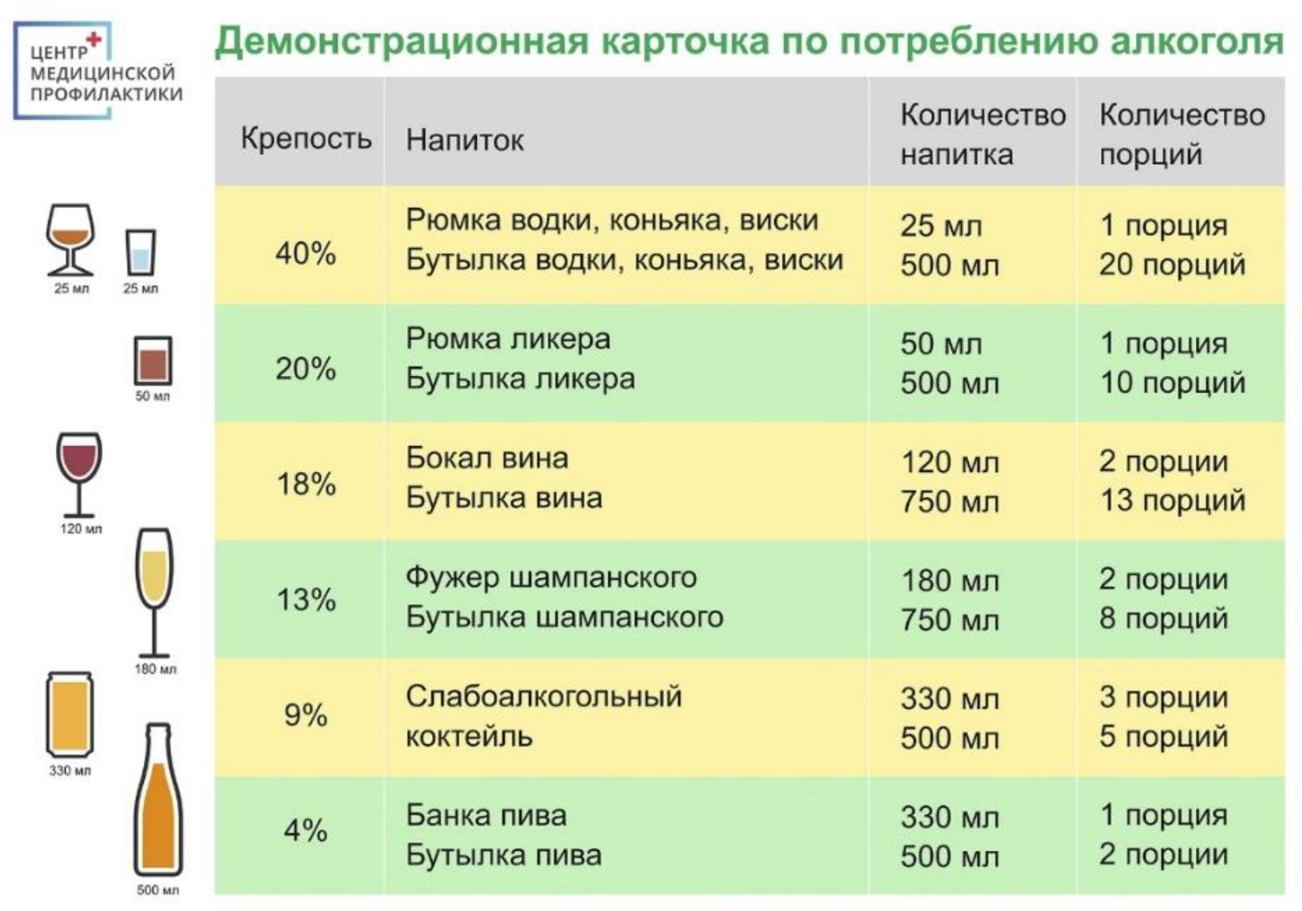
23. Looking at the alcohol consumption demonstration card, how many units (servings) of alcohol do you usually drink at a time?

	0	1-2	3-4	5-6	7-9	10+
A shot of vodka, cognac, whiskey average number of servings at a time
A shot of liqueur average number of servings per time
Glass of wine average number of servings per meal
A flute of champagne average number of servings per time
Can of beer average number of servings per time
bottle of cider, bottle of mead average number of servings at a time
Other (specify) average number of servings at a time

24. Using the same demonstration card, please answer the question: How often do you drink 6 or more units of alcohol at once?

☐ Never
☐ Less than once a month
☐ Once a month
☐ Once a week
☐ Every day and almost every day

Part (5): Socio-economic characteristics

25. In which locality do you currently reside? (e.g. Vladivostok)

26. Please write the name of the street (e.g. Nekrasovskaya St.)

____________________

27. What is your educational background? Tick the most appropriate option

9 years of school
11 years of school
Vocational education
Incomplete higher education
Higher education (Bachelor / Specialist degree)
Higher education (Master's degree)
Postgraduate education (PhD / Doctorate)
Other (please specify) ____

28. What is your father's educational background? Tick the most appropriate option

9 years of school
11 years of school
Vocational education
Incomplete higher education
Higher education (Bachelor / Specialist degree)
Higher education (Master's degree)
Postgraduate education (PhD / Doctorate)
Other (please specify) ____

29. What is your mother's education?Tick the most appropriate option

9 years of school
11 years of school
Vocational education
Incomplete higher education
Higher education (Bachelor / Specialist degree)
Higher education (Master's degree)
Postgraduate education (PhD / Doctorate)
Other (please specify) ____

30. Do you have any brothers/sisters:

☐ I am an only child
☐ One brother/sister
☐ Two brothers/sisters
☐ Three brothers/sisters
☐ Four brothers/sisters
☐ Five or more brothers/sisters

31. Please indicate your marital status:

☐ Never married
☐ Living in an unregistered marriage (cohabitation)
☐ Married in a registered marriage
☐ Divorced
☐ Widow/widower

32. Do you have children?

☐ No children
☐ One child
☐ Two children
☐ Three children
☐ Four children
☐ Five children
☐ Other ____

33. How many people live with you in the same house/apartment?

☐ One person
☐ Two people
☐ Three people
☐ Four people
☐ Five people
☐ Six people
☐ Other

34. What religion do you identify yourself as?

☐ Orthodoxy
☐ Muslim
☐ No religion
☐ Other religion

35. What is your attitude towards religion?

☐ You are a believer; you are more likely to be a believer than a non-believer
☐ You are a non-believer rather than a believer
☐ You are a non-believer
☐ You are an atheist

36. What do you currently do?

☐ Working
☐ Entrepreneur
☐ Not working
☐ Retired

37. Are you registered with the state employment service as unemployed(s)?

☐ Yes
☐ No

38. Where do you spend most of your working time?

☐ Working in a permanent job, indoors or outdoors,
☐ Working from home (telecommuting), but not online
☐ Working remotely from home or another location
☐ Working away with accommodation, shift work
☐ Working without a fixed location, travelling or moving around

39. Select from the list the industry in which you work?

☐ Light, food industry
☐ Civil engineering
☐ Defense industry
☐ Oil and gas industry
☐ Other sectors of heavy industry
☐ Construction
☐ Transport, communications
☐ Agriculture
☐ Government agencies
☐ Education
☐ Science, culture
☐ Health care
☐ Army, Ministry of Internal Affairs, security bodies
☐ Trade, consumer services
☐ Finance and insurance
☐ Energy industry
☐ Housing and utilities sector
☐ Real Estate Operations
☐ Information and communication technologies
☐ Other____

40. Please indicate how many hours per week do you work?

☐ Less than 40 hours
☐ 40 to 45 hours
☐ 46 to 52 hours
☐ More than 52 hours

41. Please specify which income category you belong to:(this is the respondent's income per month)

1. less than 15,000 rubles

2. from 15,001 and up to 30,000 rubles

3. from 30 001 and up to 60 000 rubles

4. from 60 001 and up to 90 000 rubles

5. from 90,001 and up to 120,000 rubles

6. More than 120,000 rubles

42. Which would you prefer?

☐ get 100 rubles guaranteed
☐ get a lottery ticket with which you can win 200 rubles with a probability of 50% or 0 rubles.

43. Which would you prefer?

☐ to lose 100 rubles guaranteed
☐ with a 50% chance of losing nothing or with a 50% chance of losing 200 rubles.

References

Abdallah, N. M. , et al. (2016). Analysis of accidents cost in Egypt using the willingness-to-pay method. International Journal of Traffic and Transportation Engineering, 5(1), 10–18.
Alolayan, M. A. , Evans, J. S., & Hammitt, J. K. (2017). Valuing mortality risk in Kuwait: Stated-preference with a new consistency test. Environmental and Resource Economics, 66, 629–646.
Arrow, K., Solow, R., Portney, P. R., Leamer, E. E., Radner, R., & Schuman, H. (1993). Report of the NOAA Panel on Contingent Valuation. Federal Register, 58(10), 4601–4614.
Broughel, J. , & Viscusi, W. K. (2017). Death by regulation: How regulations can increase mortality risk.
Corso, P. S. , Hammitt, J. K., & Graham, J. D. (2001). Valuing mortality-risk reduction: Using visual aids to improve the validity of contingent valuation. Journal of Risk and Uncertainty, 23, 165–184.
Ducruet, C. , et al. (2024). Ports and their influence on local air pollution and public health: A global analysis. Science of the Total Environment, 915, 170099.
Ghanem, S. , Ferrini, S., & Di Maria, C. (2023). Air pollution and willingness to pay for health risk reductions in Egypt: A contingent valuation survey of Greater Cairo and Alexandria households. World Development, 172, 106373.
Hammitt, J. K. , & Graham, J. D. (1999). Willingness to pay for health protection: Inadequate sensitivity to probability? Journal of Risk and Uncertainty, 18, 33–62.
Hammitt, J. K. , & Herrera-Araujo, D. (2018). Peeling back the onion: Using latent class analysis to uncover heterogeneous responses to stated preference surveys. Journal of Environmental Economics and Management, 87, 165–189.
Hammitt, J. K. , Liu, J.-T., & KLin, W.-C. (2000). Sensitivity of willingness to pay to the magnitude of risk reduction: A Taiwan–United States comparison. Journal of Risk Research, 3(4), 305–320. [CrossRef]
Hanemann, M. , Loomis, J., & Kanninen, B. (1991). Statistical efficiency of double-bounded dichotomous choice contingent valuation. American Journal of Agricultural Economics, 73(4), 1255–1263. [CrossRef]
Keller, E. , et al. (2021). How much is a human life worth? A systematic review. Value in Health, 24(10), 1531–1541.
Krupnick, A. (2007). Mortality-risk valuation and age: Stated preference evidence. Review of Environmental Economics and Policy.
Leiter, A. M. , & Pruckner, G. J. (2009). Proportionality of willingness to pay to small changes in risk: The impact of attitudinal factors in scope tests. Environmental and Resource Economics, 42, 169–186.
Lopez-Feldman, A. (2012). Introduction to contingent valuation using Stata.
Sajise, A. J. , et al. (2021). Contingent valuation of nonmarket benefits in project economic analysis: A guide to good practice. Asian Development Bank.
Wang, H. , & He, J. (2010). The value of statistical life: A contingent investigation in China. World Bank Policy Research Working Paper (No. 5421).
Wang, H. , & Mullahy, J. (2006). Willingness to pay for reducing fatal risk by improving air quality: A contingent valuation study in Chongqing, China. Science of the Total Environment, 367(1), 50–57.
Yeung, R. Y. T. , Smith, R. D., & McGhee, S. M. (2003). Willingness to pay and size of health benefit: An integrated model to test for ‘sensitivity to scale’. Health Economics, 12(9), 791–796.

Table 1. Levels of mortality risk reduction.

Initial risk (per 100,000)	Reduction (percentage points)	New risk (deaths per 100,000)	Reduction in absolute terms (number of deaths per 100,000 people)
1192	25	1167	25
1192	50	1142	50
1192	100	1092	100
1192	150	1042	150
1192	200	992	200

Table 2. Survey design.

Questionnaire block	Purpose
The experience of living in a seaport city	1. Stratification of respondents by place of residence: those living in a port city vs. those not living in a port city. 2. assessment of quality of life; 3. assessment of the impact of polluted air on health.
Part 2. Game questions	Identification of respondents who do not understand probabilistic changes (cognitive distortion effect)
Part 3. Scenario for assessing willingness to pay for reducing the risk of death from air pollution and attitudes toward the proposed scenario	Introduction to the problem context: Familiarization with statistics to inform respondents about the issue of air pollution and its impact on health. Random distribution of respondents into 5 groups based on the level of risk reduction (see Table 1). Determination of willingness-to-pay estimates. Identification of reasons for supporting the scenario as well as protest responses.
Part 4. Questions about health status and harmful habits	Identification of respondents who are sensitive and non-sensitive to health risks
Part 5. Socio-demographic characteristics	Population grouping by: - Age groups - Income level - Education level - Place of residence (port city/non-port city) - Employment and industry - Etc.

Disclaimer/Publisher’s Note: The statements, opinions and data contained in all publications are solely those of the individual author(s) and contributor(s) and not of MDPI and/or the editor(s). MDPI and/or the editor(s) disclaim responsibility for any injury to people or property resulting from any ideas, methods, instructions or products referred to in the content.

© 2025 by the authors. Licensee MDPI, Basel, Switzerland. This article is an open access article distributed under the terms and conditions of the Creative Commons Attribution (CC BY) license (http://creativecommons.org/licenses/by/4.0/).

Copyright: This open access article is published under a Creative Commons CC BY 4.0 license, which permit the free download, distribution, and reuse, provided that the author and preprint are cited in any reuse.

Development of Economic and Mathematical Tools for Analyzing and Evaluating the Value of Life Based on Willingness to Pay for Mortality Risk Reduction (Using Air Pollution as an Example)

Abstract

Keywords:

Subject:

Introduction

Literature Review

Methods and Data

Study Design

Conflicts of Interest

Appendix A

References

MDPI Initiatives

Important Links

Subscribe