Submitted:
10 February 2025
Posted:
12 February 2025
You are already at the latest version
Abstract
Hyalesthes obsoletus, a planthopper of the family Cixiidae, is a very efficient vector of the phytopathogenic bacterium ‘Candidatus Phytoplasma solani’, which causes diseases in a variety of crops, including grapevines. The larvae are oligophagous and infect their host plants, in Central Europe mainly Convolvulus arvensis and Urtica dioica, the polyphagous adults transmit the pathogen both to the hosts of the larvae and to the crop plants, which are dead-end hosts in the infection process. In this study, characteristics of the larval stages are analysed comparatively. Body length, length of the antenna, the labium and the metathoracic limb were determined for the five instars and conclusions drawn about changes in proportions. Furthermore, the morphology of the antennae was described, the development of the eye primordium, the distribution of the sensory pits on the pro-, meso- and metanotum, the alteration of the tarsi and other features of the hind legs (‘gear-teeth’ as in Issus are present) and the structure of the wax plates of the abdomen during individual development. The characteristics of these features were summarised in a table and allow a reliable instar classification. The easiest way to do this is with the aid of the wax plate, which is divided mediolaterally into several sections by sensory pits. This results in a simple relation: Instar = number of wax plate sections – 1. The results are compared in particular with the description of the larval stages by Sforza et al. 1999. Larval development is relevant for the beginning of the flight period and thus also for the start of pathogen spread in the course of the year.
Keywords:
planthopper
; Hemiptera
; Auchenorrhyncha
; Fulgoromorpha
; Cixiidae
; Hyalesthes obsoletus
; larval development
; instar description
Introduction
The Palaearctic planthopper Hyalesthes obsoletus Signoret (Hemiptera, Cixiidae), is an efficient vector of the phytopathogenic bacterium ‘Candidatus Phytoplasma solani’ (taxonomic subgroup 16SrXII-A) of the order Acholeplasmatales within the class Mollicutes (Quaglino et al., 2013), the causal agent of, among others, the Bois noir disease of grapevine. In contrast to the soil-dwelling larvae of H. obsoletus, which are restricted to a relatively narrow host range (Urtica dioica and Convolvulus arvensis in Germany, Italy and Austria, Cardaria draba, Lavendula spp. in France, Vitex agnus-castus in Israel, Crepis foetida in Serbia and some others), the adults are polyphagous and can therefore transmit the pathogen from the host species, on which roots the larvae feed, to a wide range of cultivated and wild plants, including grapevines. The pathogen has a very broad host range of more than 90 wild and cultivated plant species from 36 families and causes significant damage in some crops. Infection is also often an incidental side effect of the vector testing the suitability of a plant as food.
Due to their limitation to a few reproductive hosts, the larvae themselves are not able to acquire phytoplasmas from or pass them on to cultivated plants. As a result, crops are always the dead-end hosts in epidemic cycles with H. obsoletus as the pathogen vector (Johannesen et al., 2008; Jovic et al., 2019).
In Western and Central Europe, the stinging nettle Urtica dioica and the field bindweed Convolvulus arvensis are of particular importance for the epidemiology of Ca. P. solani as they are almost always the source of the phytoplasmas and the infection therefore originates from them (Langer and Maixner, 2004; Aryan et al., 2014; Landi et al., 2015). Accordingly, analysis of the gene sequences of the elongation factor TU of ‘Ca. P. solani’ strains has identified two major lineages, tuf-a and tuf-b, which are associated with U. dioica and C. arvensis, respectively. In practice, there are two independent epidemic cycles with these two hosts (Langer and Maixner, 2004). Studies in Austria have also shown that a genealogical intermediate between the types tuf-a and tuf-b, namely tufb2, is associated with U. dioica (Aryan et al., 2014).
As early as 1981, on the basis of genetic investigations Imo came to the conclusion that H. obsoletus had also developed host-specific races. A genetic analysis using random amplification of polymorphic DNA and simple sequence repeat markers on this species also revealed evidence of genetically distinct, host-specific populations, i.e., host races (Johannesen et al., 2008; Imo et al., 2013). This is significant in that all the larvae analysed here developed on the roots of stinging nettles and the results of this analysis therefore do not necessarily apply to the second variant of H. obsoletus.
Apart from its importance as a vector of Ca. P. solani, H. obsoletus is rather unspectacular. It is a small (3-6 mm), dark-coloured, usually not very common, but tending to occasional mass reproduction, fulgoromorph and as an adult polyphagous planthopper that sucks on the phloem of its host plants. The distribution covers the Mediterranean and extends northwards and eastwards to Germany and Russia. It is more common on embankments and roadsides than in vineyards. As an adult, this species lives for a maximum of six weeks in June and July. The females lay their eggs in the soil near the hosts of the oligophagous larvae, which feed on the roots and live in the soil. 25 overwintering hosts have been identified in the entire distribution area to date. Five larval stages are formed, which were described in detail by (Sforza et al., 1999). An identification key is available. The present study is intended to provide additional information that is useful for a reliable classification of the instars.
This should make it possible to estimate the predictive accuracy of existing models with regard to larval development and, in particular, the time of moulting to the adult or the onset of flight and thus the spread of the pathogen over the course of the year, or to make model corrections if necessary. The models of Maixner & Langer 2006 and Maixner and Johannesen 2014 are based on temperature sums and are used in the integrated control of Bois noir.
Method
As part of the StolReg project (control of Stolbur phytoplasma pathogens in potato, vegetable, sugar beet and vine cultivation), immature H. obsoletus individuals of unknown quantity from the collection of M. Riedle-Bauer (HBLAWO Klosterneuburg) were made available for the investigation of larval development. The larvae were overwintered in the root ball of nettles in four plastic plant pots (height 28 cm; diameter 20 cm at the top and 16 cm at the bottom) in a weather-protected but unheated storage room. At the end of March (22 March), they were transported to two locations near Donnerskirchen (Burgenland, Austria), site Goldberg and site Wolfsbrunnbach. The contents of the pots (host plant, potting soil and larvae; hereafter referred to as the experimental unit), but not the pots themselves, were placed surrounded by a water-permeable synthetic net in the ground near weather stations (ADCON-Ott) and vineyards, two per site. In order to obtain additional Hyalesthes specimens, soil samples were taken at weekly intervals at Donnerskirchen, site Goldberg, not far from the experimental unit, and in Rust (Burgenland, Austria), in each case in an Urtica dioica stand. The soil animals were extracted using a Berlese funnel system. The specimens collected in this way were stored in 75% alcohol, as were those taken weekly from the experimental units. If the latter were successful (which was not always the case), they were immediately preserved on site.
Prior to analysis, the animals were brightened with Mark Andre I and then prepared in Mark Andre II on a slide using a Zeiss Stemi 2000-C microscope. The analyses were carried out with a Zeiss Axio-Imager.A2 microscope in bright light, phase contrast and interference contrast. Survey data from 48 individuals were available for evaluation, which were divided into the following groups according to the date of sampling: 22 March (2 individuals); 23 March (12 individuals); 5 April (5 individuals); 20 April (5 individuals), 4 May (6 individuals), 16 May (4 individuals); 2 June (6 individuals) 17 June (4 individuals); 28 June (4 individuals). It is likely that there was a delay in development in the experimental units due to a severely reduced vitality of the host, because adults were already found on outdoor sticky traps before mid-June, but larvae were still present in the experimental units till the end of the month. However, it can only be surmised whether the reduction in host vitality was a consequence of parasitisation, of hibernation in the pot, or whether it was caused by the restriction of root growth due to the synthetic net.
The biometric analysis was carried out using the microscope mentioned above, equipped with a mechanical stage for moving objects and quantifying object movement plus a sensor control display. This equipment was supplemented by user software which made it possible to measure in two dimensions, while differences in the third dimension (top - bottom) remained undetermined.
For statistical analysis (comparison of the twelve groups differing by date of sampling and/or location), a Multiple Range Test, 95% LSD was carried out using Statgraphics Centurion XV. This test assigns the data to homogeneous groups, the number of which should correspond to the number of larval instars. Box and whisker plots were chosen as the form of visualisation.
Results and Discussion
- Biometric studies on the instars
Sforza et al. 1999 described the instars of H. obsoletus mostly qualitatively, but the publication also contains biometric data (body length, body width, thorax length, head length, head width). However, there is no precise description of the measurement procedure, such as the choice of front and end point of the measurement, or a corresponding scheme. Comparability with the data collected here would therefore be limited, which is why – apart from the body length – other structures were measured. The morphology of a species is always variable to a certain degree and could depend on external factors, such as the temperature during development or the host species and thus the nutritional status. In the study carried out in France, the immature individuals were grown on lavender or field bindweed at 23°C, whereas here they were grown on stinging nettle in the weather conditions prevailing at the site. It is therefore advisable to check whether the biometric data also apply to the local conditions. The following body parts were selected for measurements:
Total length of the individual: Due to the stretchable intersegmental integument, this characteristic is critical and is only used for comparison with the above-mentioned publication. The animals were measured between slide and coverslip, i.e., in a crushed state. For a more detailed definition of the term ‘total body length’, see Figure 1.
A total of 38 of the 48 individuals from twelve groups differing according to the date of sampling and/or location (hereinafter referred to as clusters) were measured for a habitus comparison and then subjected to a Multiple Range Test for mean comparison. The test procedure divides the clusters into five Homogeneous Groups and it turns out that they correspond to the five instars ((verified with the description of non-metric characteristics according to Sforza et al. 1999). This is remarkable because the test procedure has no a priori knowledge of the assignment of individuals to the larval stages. Results of the statistical procedure and the published data are shown in Table 1.
The specimens of the first Homogeneous Group (HG1) correspond approximately to the body length of instar L2 in the analysis of Sforza et al. 1999 (about 0.99 mm), but actually belong to L1. According to the authors, L2 is the hibernation stage, but apparently L1 individuals can also hibernate. HG2 (and correspondingly L2) includes 25 individuals from five clusters with an average size of 1.6 mm, which fits the body length of the L3 instar by Sforza et al. 1999. The animals are on average slightly longer than indicated for the third instar, but fit into the described range. HG3 (N=2), the third instar, has a length of 2.2 mm, which again corresponds well with the data for L4 in the cited article. The comparison of HG4 (N=7), the fourth instar, and L5 according to Sforza et al. 1999 also shows a good agreement, which is made possible by the extremely large range of variation (over 1 mm at 3 mm body length!) of the French L5 individuals. The same also applies to the, compared to HG4, much larger HG5 (L5-instar) individuals (N=2). Overall, it can therefore be concluded that the individuals analysed here are larger at the same instar and correspond approximately to the next stage of the population described by Sforza et al. 1999.
Figure 2 shows the affiliation of the clusters to the Homogeneous Groups and the distribution of body length within the clusters. This in turn allows conclusions to be drawn about growth (Figure 3). According to this, the body length would grow linearly (i.e., by a constant amount from group to group), which is extremely unlikely. The extensibility of the intersegmental integument during preparation may have played a role here.
The present biometric analysis suffers from the fact that some instars were represented by only a few individuals. Supplementary sampling (a total of seven samples at two locations) on 6 October of the study year to obtain additional L1s was unsuccessful with regard to the larvae of H. obsoletus, as were collections in the autumn of the previous year (22 samples). Despite the small sample size in some cases, the authors believe that the results are sufficiently interesting to justify publication as a preprint.
Total antenna length: Scapus (A1), pedicellus (A2), the bulbous funiculus (the first flagellum section A3) and the rest of the flagellum (Arista) were measured separately and the respective contributions to the antenna length were added. The problem in this case was that the antenna has the property of bending upwards and the third spatial axis cannot be measured. This is particularly important in later larval stages, where the distance between the slide and the cover glass is increased.
There is no comparative data for this feature in the publication by Sforza et al. 1999. Bourgoin & Deiss 1994 provide a description of the antenna of the Cixiidae, but do not refer to H. obsoletus and do not carry out any measurements. Romani et al. 2009 describe the antenna of the adult. The sample size situation is somewhat more favourable here, as both antennae were analysed in most individuals. A total of 51 antennae were measured.

Table 2.
Length of the antennae. Assignment of data to Homogeneous Groups by Multiple Range Test for mean comparison. With one exception, this corresponds to the instar affiliation.
Table 2.
Length of the antennae. Assignment of data to Homogeneous Groups by Multiple Range Test for mean comparison. With one exception, this corresponds to the instar affiliation.
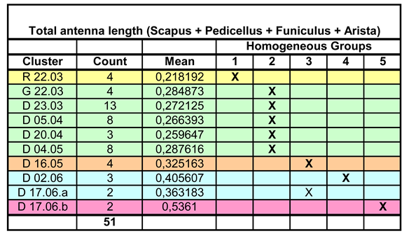 |
Compared with the analysis of body length, there is a significant difference, namely the assignment of D 17.06.a (a cluster was divided into a and b if two instars were in the same root ball at the same time) to HG3 instead of HG4. This is probably due to the fact that the antennae, especially in later larval stages, curve upwards and the vertical dimension cannot be measured. The length of the flagellum can then be underestimated. According to the graphical representation in Figure 5, however, D 17.06.a would rather be assigned to HG4 and thus L4, which would be correct. The data distribution certainly plays a role here.
Figure 6 shows the correlation between antenna length and Homogeneous Group. This suggests that the characteristic grows exponentially, i.e., that each instar increases by an amount proportional to the previous one. This assumption is much more plausible than that of linear growth. In the course of larval development, the antennal length decreases more and more relative to the body length, thus showing negative allometric growth and resulting in a proportional shift. This relative decrease is the cause of the problems with measurement in later instars because the distance between the slide and the cover glass increases and the relatively small antenna can therefore bend upwards more strongly.
Labium: In the Auchenorrhyncha, the labium (maxilla II) has been remodelled into a guiding groove for the sucking spines (remodelled mandibles and maxillae I). The most proximal element, the submentum (SM), the medial mentum (M) and the distal postmentum (PM) were measured separately and later added to the total length of the labium (Figure 7).
There are no comparative values for the length of the labium in the publication by Sforza et al. 1999. 42 individuals were measured (Table 3). Since the labium at rest is parallel to the sternites, i.e., to the ventral region, the measurement is much less problematic than was the case with the antenna.
Table 3.
Length of the labium. Assignment of the data to Homogeneous Groups by Multiple Range Test. For two clusters the assignment is not unequivocal.
Table 3.
Length of the labium. Assignment of the data to Homogeneous Groups by Multiple Range Test. For two clusters the assignment is not unequivocal.
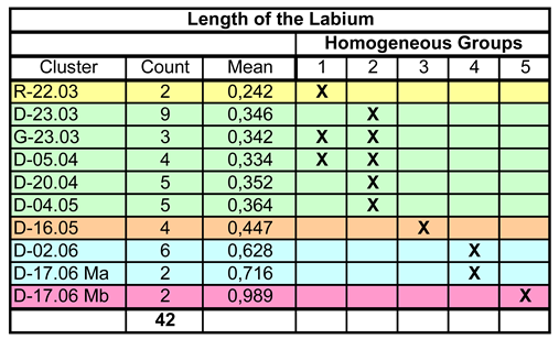 |
Nevertheless, there are deviations in the allocation to the Homogeneous Groups that affect two clusters. For G-23.03 and D-05.04, the assignment to HG1 or HG2 is not clear, i.e., there is no significant difference to R-22.03 or e.g., D-23.03, although the last two clusters differ significantly from each other. This could be due to the variance of the measurement data, but more likely to the small sample size. The latter is supported by the following figure, which compares the medians and quantiles of the clusters. No difficulties can be seen here in the allocation of G-23.03 and D-05.04; the affiliation to HG2 appears clear.
The growth of this feature is exponential, as is the case with the antenna, only that the labium grows faster, i.e., the exponent is correspondingly larger. In comparison to the body length, the labium therefore remains relatively longer than the antenna during development.
Figure 9.
Comparison of labium length in the instars (Homogeneous Groups of the statistical analysis).
Figure 9.
Comparison of labium length in the instars (Homogeneous Groups of the statistical analysis).

Limb of the third thoracic segment. The two most proximal elements of the hind leg, coxa and trochanter, were not included in the measurement (because they are very short and therefore difficult to measure). The biometric analysis therefore includes the femur, tibia and tarsus in their entirety. The three sections were measured separately (from condyle to condyle or tip), as shown in the following figure, and the results were added to the “leg length”. The procedure proved to be quite straightforward.
Figure 10.
Femur, tibia, and multi-articulated tarsus of the hind leg.
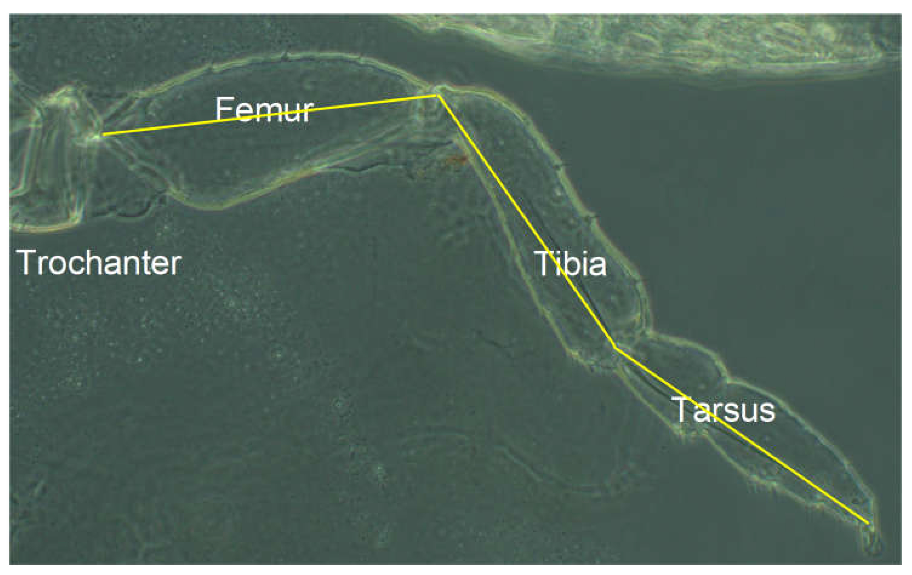
To determine the length of the metathoracic limb, 64 hind legs were measured, but the sample size is small in some instars. The legs are generally parallel to the body axis and can therefore be easily analyzed with a two-dimensional measuring device. Comparative values do not exist. The result of the Multiple Range Test is shown in the following table.
Table 4.
Length of the metathoracic limb. Assignment of the data to Homogeneous Groups by the Multiple Range Test.
Table 4.
Length of the metathoracic limb. Assignment of the data to Homogeneous Groups by the Multiple Range Test.
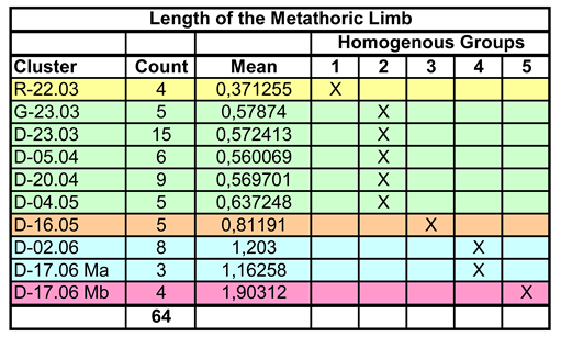 |
Once again, five homogeneous groups are formed (the number is not predetermined by the method, but results from the data), the assignment of the clusters is unequivocal. This is mainly due to the fact that the low variance compensates for the often limited sample size. This is also confirmed in the graphical representation (Figure 11).
The growth from stage to stage is again exponential, whereby the goodness of fit (the coefficient of determination R2) is very high, as in all cases examined (Figure 12).
As already mentioned, there are shifts in proportions during the growth of H. obsoletus. These can be compared and quantified by plotting the exponential coefficients of the previous analyses (shown in Figure 6, Figure 9 and Figure 12) together (Figure 13).
Obviously, the metathoracic limb, the “jumping leg” of the cicada, grows faster than the labium and especially than the antenna, which finally appears relatively small at the fifth instar, just as in the adult.
A multivariate analysis using PCA (Principal Component Analysis) was carried out on the basis of eleven body features (body length, four antenna features, three labium characteristics and three hind leg ones), which are listed in the margin of the following diagram (Figure 14). 87 objects are compared, whereby in many cases two objects correspond to one individual; these are then the two bilateral body halves.
As can be seen, only the first principal component allows a separation of the Homogeneous Groups, although this is very successful: All 87 objects are correctly assigned. The fact that only one of the principal components has assignment information indicates the high correlation of all features.
- Comparison of stages and morphological description of some body features
The feature complexes are described from anterior to posterior along the longitudinal body axis:
General description of the antenna: The antenna of H. obsoletus, which is inserted laterally on the head capsule, is divided into scapus (A1; basalmost antennal segment), pedicellus (A2) and flagellum, as in all pterygote insects. However, here the flagellum is further subdivided into a bulbous, basal element, the funiculus (A3), an adjacent, non-segmented section, followed by a segmental one and finally a narrowly annulated terminal section (see following photograph and diagram, Figure 15). The flagellum without funiculus is also called arista, which inserts on the funiculus, as well as a candle-shaped spur. The antenna usually protrudes laterad from the head, but can also be placed posteriorly on the body. It is located ventral to the eye primordium, if one is already visible. In the imago, the antenna is about 750 μm long, the pedicellus 150 μm and the flagellum 500 μm, of which the arista accounts for about 440 μm (according to Romani et al. 2009).
The pedicellus and funiculus are of particular interest because they are the carriers of different sensory organs (presumably tactile and olfactory exteroceptors and hygro- and osmoreceptors), see Figure 16 (different instars are shown):
The antenna of the first instar (L1): Scapus and pedicellus are free of antennae-typical sensory organs. A3 (funiculus) is only slightly narrower and somewhat longer than A2 (pedicellus). Distally on the funiculus - not far from the base of the residual flagellum - there is an elongated (≈2/3 of the funiculus length) appendage, which is referred to here as a candle-shaped organ, but in Romani et al. 2009 as a “spur”, whereas the “wick” of the “candle” is referred to as a “peg”. In the adult it is tripartite (three “wicks” next to each other), perhaps also in the larvae, but this cannot be clearly seen under the light microscope. A spherical organ can also be observed at the base and a mushroom-shaped one nearby, somewhat proximal to it. Both are not mentioned by Romani et al. 2009; they are therefore either regressed in the adult or are lost as a result of preparation for scanning electron microscopy. At this location they recognize an aperture. They write: “... the bulb of the flagellum revealed two cuticular cavities opening at the level of the external aperture located at the base of the cuticular spur”. It is therefore more likely that this is an artifact of the preparation than a reduction.
A little further proximal - already close to the funiculus equator - an anemone-shaped organ with several projections (around six) is visible. It is described by Bourgoin & Deiss 1994 and Sforza et al. 1999 as “plate organ” and by Romani et al. 2009 as “sensillum placodeum”. Even further proximal is a pair of lyre- to rod-shaped sensilla, which are similar in length to the candle-shaped organ (i.e., considerably longer than the usual sensory hairs distributed over the entire body surface). They are no longer found in the adult. The remaining flagellum, the arista, has three clearly separated segments between the unstructured basal and distal sections.
The antenna of the second instar (L2): A3 is about half as wide as A2 and slightly shorter. The funiculus (A3) is almost the same as before, but the anemone-shaped organ is simplified or even completely reduced (Figure 17). The sensory field (anemone-shaped organ and lyre-shaped sensilla) moves further away from the funiculus equator as part of a proportional shift. The pedicellus (A2) is now adorned with three anemone-shaped organs with about nine projections.
The antenna of the third instar (L3): A3 is at most 1/3 as wide as A2 and at maximum half as long. On the funiculus, the anemone-shaped organ and the pair of lyra-shaped sensilla are now completely reduced. On the pedicellus, in addition to four simpler anemone-shaped organs in the distal position, there is a sensilla area (approx. 12 trichia, described by Romani et al. 2009 as “Sensilla trichodea”).
The antenna of the fourth instar (L4): There are now six clearly separated segments on the residual flagellum (the arista) between the basal and distal sections. A3 is approx. 1/3 as long as A2. The funiculus (A3) is almost unchanged compared to the previous stage. Distally on the pedicellus a field has developed that is very densely occupied by finger-shaped organs ((they are not mentioned by Romani et al. 2009). This shifts the sensilla area (Sensilla trichodea) further proximad. It now comprises about 20 trichia. A2 now bears eight well-developed anemone-shaped organs (four in the foreground and four in the background in Figure 17).
Figure 17.
Schematic representation of the antennae in the different instars.
The antenna of the fifth instar (L5): The flagellum remains almost unchanged. A3 approx. ¼ as long and maximally ¼ as wide as A2. On the pedicellus, the sensilla field has expanded dorsad and now accommodates approx. 40 trichia. The field with finger-shaped organs has not changed significantly. The now ten anemone-shaped organs are partly located at the edge of the sensilla area, but never within it.
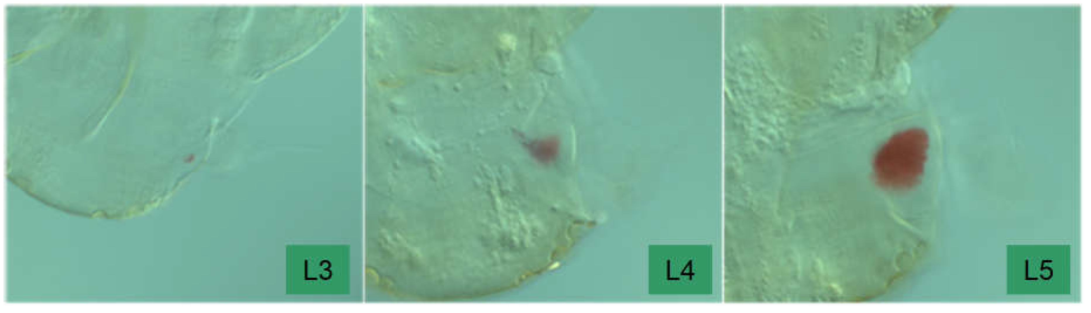
Description of the eyespot: The ocular primordium is only recognizably present since the third instar, before that there is a trichobothrial area (a field of “sensory pits” sensu Sforza et al. 1999) dorsal to the antenna base. In L3, at best a slight pigment formation indicates the place where an eye will once be ((Sforza et al. 1999 describe this as follows: “ocular structure represented by three poorly developed red circular facets; no compound eyes”). In L4 individuals, there is a clear pigment spot (red), but it is narrower than the base of the scapus (“compound eyes represented by fewer than ten poorly developed, red circular facets”). A spherical bulge is also barely visible. This changes in L5. Here the contours of the compound eye are already clear and the pigment spot is as large or even larger than the base of A1.
Figure 18.
The development of the eyespot from the third to the fifth instar.
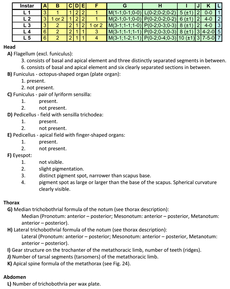
Description of the thorax (dorsal): In the dorsal region of the thorax there are small cuticle pits ((“sensory pit” of Sforza et al. 1999; here: trichobothrium) in all instars, each of which houses a single, long sensory hair with a lance-shaped tip. The base of the hair is not located centrally in the pit but laterally, the trichium is often oriented posteriorly. They can vary in size, “younger” ones are somewhat smaller. The trichobothria form a pattern on the nota that changes in the course of development. In addition to a median stripe of countable trichobothria, there is at least one double trichobothrium laterally on the nota, followed by the trichobothrial area of the paranota, in which a large number of sensory pits lie quite close together. Due to their lateral position alone, they are less suitable for rapid assignment to an instar. In the median position there are 0 to 3 trichobothria on the anterior and posterior edge of each thoracic segment on each side of the body. This can be summarized in a formula, e.g., Median(Pronotum: 3 anterior - 1 posterior; Mesonotum: 1 anterior - 1 posterior, Metanotum: 1 anterior - 0 posterior) becomes: M(3-1;1-1;1-0). The same is done for lateral L, but not for the paranota. See also Figure 19.
Note that in the pronotum the lateral trichobothria are directly adjacent to the paranotal trichobothrial area and can form rows with it. In individual cases there are left-right asymmetries (a missing or additional trichobothrium). The following illustration shows the comparison of instars:
Figure 20 shows only a partial correspondence with the habitus illustrations of Sforza et al. 1999. It is therefore possible that population-specific deviations occur in the trichobothria pattern. In any case, the coding for the specimens examined here is as follows:
Nota & paranota in L1: M(1-1;0-1;0-0), L(0-2;0-2;0-2). Paranota are not extended posteriad to wing anlagen.
Nota & Paranota in L2: M(2-1;0-1;0-0), L(0-2;0-2;0-2). Paranota are not extended posteriad to wing anlagen.
Nota & paranota in L3: M(3-1;1-1;1-0), L(0-2;0-3;0-3). Meso-paranota with a beginning development into a wing anlage: the posterior margin of the notum shield overlaps the anterior margin of the metanotum.
Nota & paranota in L4: M(3-1;1-1;1-1), L(0-2;0-3;0-3). Mesonotum with distinct wing anlagen, metanotum overlapping the anterior abdominal margin.
Nota & paranota in L5: M(3-1;1-2;1-1), L(0-2;0-4;0-3). Mesonotum with well-developed wing anlagen, extending much further posteriad than to the median posterior margin of metanotum. Distinct wing anlagen are also developed on the metanotum.
Description of the metathoracic limb: Compared to the pro- and mesothoracic limbs, the coxa is very short. The trochanter has a conspicuous structure (“gear-teeth”), which was first described for the genus Issus (Fulgoromorpha) (Burrows & Sutton, 2013). The gear-like structure on the trochanter of the hind leg also exists in H. obsoletus larvae (Figure 21). The structure is thought to serve to synchronize leg movement during jumping. Although the larvae have little opportunity to jump as bottom dwellers, they still have this feature and can actually jump well. The upper left partial figure shows the “gears” in the unlocked state, the right one in the locked state, where they connect the two trochanters. The lower row of images shows the structure from different perspectives.
L1: The trochanter carries five ridges (“teeth”) that run more or less parallel and become higher from posterior to anterior.
L2: Like L1, but generally with six ridges.
L3: Generally eight ridges are formed.
L4: like L3.
L5: Generally with 10 teeth.
Femur and tibia are very long in later instars (“ jumping leg”). The tarsus changes in the course of development. Apart from the claw-bearing last segment, its sections have apical spines at the distal end, which in the first two instars can be mistaken for sensory hairs in terms of size. However, they are rigid, while the hairs are passively movable in a circular base. The integument here has a thin cuticle (Figure 22: The upper right partial illustration shows a sensory hair, the lower right one an apical bristle).
The following illustrations (Figure 23) show the tarsi in various stages of development (two partial illustrations also show the tibia).
A schematic presentation and a verbal description follow:
L1: Tarsi of pro- meso- and metathorax uniformly bipartite. Metathoracic tarsus without apical spines.
L2: Metathoracic tarsus bipartite, basal segment more distinct than in L1 and with four apical spines. A small spine on the distal tarsomer in the position where the division into two segments will take place later.
L3: Like L2, the two tarsal segments are even more clearly separated.
L4: Metathoracic tarsus in contrast to pro- and mesothoracic tarsus tripartite, from proximal to distal with 5, 2, 0 apical spines (see Figure 24).
L5: Metathoracic tarsus tripartite, apical spine formula: 7, 5, 0.
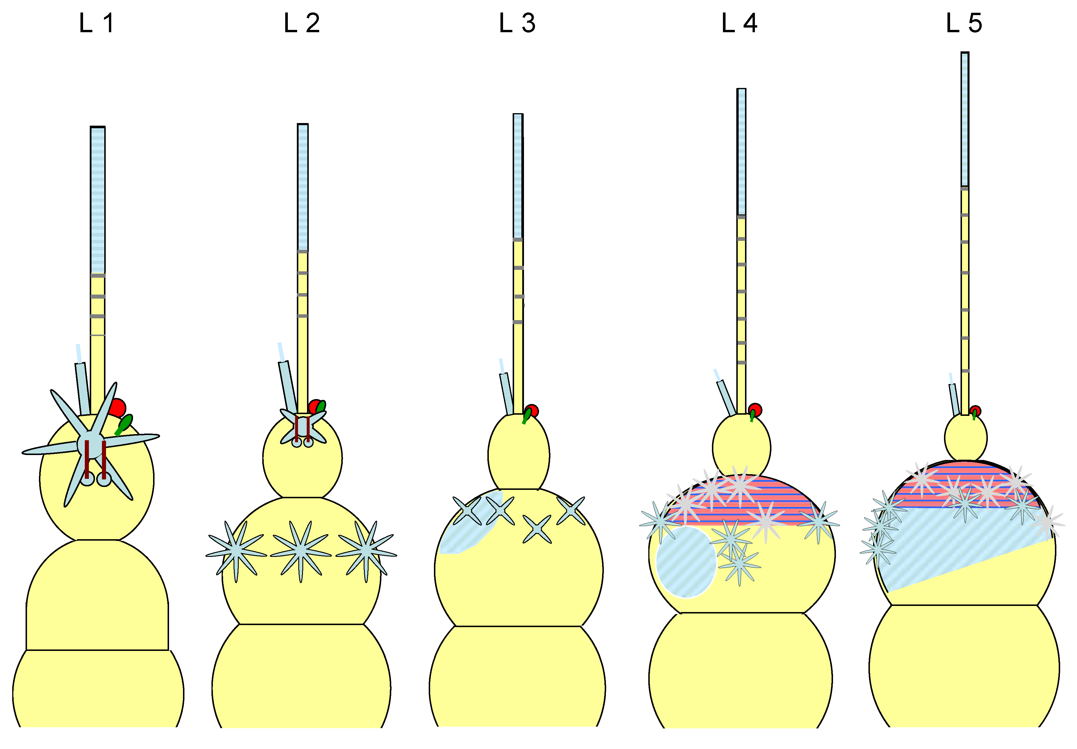
Abdomen - wax plates: The larvae often carry white wax brushes of up to body length on the tip of the abdomen. The filaments are produced by wax plates ((sensu Sforza et al. 1999), which are located on segments VI to VIII of the abdomen. As shown schematically in Figure 25, they do not only consist of wax glands. Sforza et al. 1999 write about these: ‘Glandular units are more complex, flower-like and similar to those already described in another cixiid, Myndus crudus by Pope (1985). Each glandular unit consists of a central circular area almost 5 μm in diameter surrounded by a circular ridge with 5-8 white pits (...). Each pit is externally bordered by a petal-like ornamentation on the internal base of which are a pair of pores, 0,8 μm in diameter ... ‘. This is indicated in the following diagram.
Further important components of the wax plates are sensory organs, simple sensilla on the one hand and sensory pits with one hair each, trichobothria, on the other. Two wax plates are present per segment in a bilateral arrangement. The wax plates are basically the same in the three segments, they only become slightly narrower posteriorly. The wax gland units do not form clear rows. A less schematic representation of a wax plate (L1) is shown in the next figure (Figure 26). The upper photograph was taken in phase contrast, the lower one in interference contrast. Contrary to the schematic, the wax plates are not symmetrical; fewer wax gland units are formed medially of the trichobothrium than laterally.
L1: Wax gland corona (the sheath-like margin of the wax gland unit) predominantly five (4-6)-partite, the wax gland units three-rowed in anterior-posterior extension. A trichobothrium (the lance-shaped ending of the sensillum is orientated posteriad) divides the wax plates from medial to lateral into two not quite symmetrical parts (medial < lateral). Each of these parts contains a simple sensillum, approximately as far away from the Trichobothrium as this is wide. The wax plate is distinctly framed.
L2: Wax gland corona mostly six-parted (or more), the wax gland units form four rows in anterior-posterior extension, the wax plate thus grows in this dimension. It is divided into three sections by two trichobothria, each containing a sensillum. The middle section consists of more than 20 wax gland units. The trichobothria, which apparently do not grow from moult to moult, remain in the anterior position, i.e., they no longer divide the wax plate completely (Figure 27).
L3: The wax plate is divided by three trichobothria into four sections, each containing a sensillum. The longitudinal-section (anterior-posterior) is six to seven rows of wax gland units. The trichobothria are positioned anteriorly and are about half as long as the wax plate in anterior-posterior extension. A groove is formed in this direction at each trichobothrium, which remains free of wax gland units.
L4: The wax gland corona is usually eight-parted. The anterior-posterior longitudinal-section of the wax plate is about eight wax gland units wide. The wax plate is divided by four rows of trichobothria into five parts, each containing a sensillum. The wax gland-free groove at the trichobothrium is now very distinct. There is a clearly recognisable asymmetry, as the most lateral furrow contains two trichobothria located one behind the other, the posterior one of which is slightly laterally offset.
L5: the wax plate is divided by five rows of trichobothria into six sections, each of which contains a simple sensillum. The asymmetry is increased compared to L4, the two most lateral trichobothrial grooves each contain two trichobothria one behind the other, in the most lateral furrow the posterior trichobothrium is slightly offset laterad, but not in the neighboring one, where the two trichobothria are positioned exactly one behind the other.
Overall, the following simple relationship results:
Instar = number of wax plate sections -1
As the wax plates grow with the molts, it is unlikely that a trichobothrium will be dissolved and replaced by one elsewhere. The rather complex organs will be preserved and one can now consider what the correspondence is for successive stages. It is most likely that the addition of new material is mainly lateral and posterior (red arrows), as indicated in the next figure (Figure 27), which compares the instars.
In the following, the schematic representation will be compared with the actual conditions in a photo series. Figure 28a (interference contrast) and Figure 28b (phase contrast) show the wax plate in L2, Figure 28c shows the abdominal median in L3 and is a section from Figure 28d. Figure 28e and Figure 28f show trichobothrial grooves in the fourth instar, a median one in Figure 28e and a lateral one in Figure 28f.
In the following table and list, the characteristics are compared with the stages:
With the aid of Table 5, a reliable classification of the instars of H. obsoletus is possible.
Acknowledgments
This work was financially supported by the StolReg project (control of Stolbur phytoplasma pathogens in potato, vegetable, sugar beet and vine cultivation). We thank M. Riedle-Bauer for the animals provided and K. Wechselberger for her support during the fall collections.
References
- Aryan, A., G. Brader, J. Mörtel, M. Pastar, and M. Riedle-Bauer. 2014. An abundant ‘Candidatus Phytoplasma solani’ tuf b strain is associated with grapevine, stinging nettle, and Hyalesthes obsoletus. Eur. J. Plant Pathol. 140: 213–227. [Google Scholar] [CrossRef] [PubMed]
- Burrows, and & Sutton. 2013. Interacting Gears Synchronize Propulsiv Leg Movements in a Jumping Insect. Science 341: 1254–1256. [Google Scholar] [CrossRef] [PubMed]
- Maixner, M., and M. Langer. 2006. Prediction of the flight of Hyalesthes obsoletus, vector of stolbur phytoplasma, using temperature sums. IOBC-WPRS-Bulletin 29, 11: 161–166. [Google Scholar]
- Maixner, M. 2014. Johannesen, Optimized monitoring of host populations of the Bois noir vector, Hyalesthes obsoletus, based on flight phenology observations. IOBC-WPRS-Bulletin 105: 151–157. [Google Scholar]
- 2022. Mehle, N., Kavcic, S., Mermal, S., Vidmar, S., Novak, M.P., Riedle-Bauer, M., Brader, G., Kladnik, A. & Dermastia, M. Geographical and Temporal Diversity of ‘Candidatus Phytoplasma solani’ in Wine-Growing Regions in Slovenia and Austria. Frontiers in Plant Science 13: 889675. [CrossRef] [PubMed]
- Imo, M. 1981. Host race formation in Hyalesthes obsoletus (Signoret 1865), Dissertation of the Johannes Gutenberg-University in Mainz. [Google Scholar]
- Imo, M., M. Maixner, and J. Johannesen. 2013. Sympatric diversification vs. immigration: deciphering host-plant specialization in a polyphagous insect, the stolbur phytoplasma vector Hyalesthes obsoletus (Cixiidae). Mol. Ecol. 22: 2188–2203. [Google Scholar] [CrossRef] [PubMed]
- Johannesen, J., and M. Riedle-Bauer. 2014. Origin of a sudden mass occurrence of the stolbur phytoplasma vector Hyalesthes obsoletus (Cixiidae) in Austria. Ann. Appl. Biol. 165: 488–495. [Google Scholar] [CrossRef]
- Jovic, J., M. Riedle-Bauer, and J. Chuche. 2019. Edited by Bertaccini, P. Weintraub and G. Rao. Vector role of cixiids and other planthopper species. In in Plant Pathogenic Bacteria-II. N. Mori (Singapore: Springer): pp. 79–113. [Google Scholar] [CrossRef]
- Landi, L., P. Riolo, S. Murolo, G. Romanazzi, S. Nardi, and N. Isidoro. 2015. Genetic variability of stolbur phytoplasma in Hyalesthes obsoletus (Hemiptera: Cixiidae) and its main host plants in vineyard agroecosystems. J. Econ. Entomol. 108: 1506–1515. [Google Scholar] [CrossRef] [PubMed]
- Langer, M., and M. Maixner. 2004. Molecular characterisation of grapevine yellows associated phytoplasmas of the stolbur-group based on RFLP-analysis of non-ribosomal DNA. Vitis 43: 191–199. [Google Scholar] [CrossRef]
- Pope, R.D. 1985. Visible insect waxes, function and classification. Antenna 9: 4–8. [Google Scholar]
- Quaglino, F., Y. Zhao, P. Casati, D. Bulgari, P. A. Bianco, W. Wei, and et al. 2013. ‘Candidatus Phytoplasma solani’, a novel taxon associated with stolbur-and bois noir-related diseases of plants. Int. J. Syst. Evol. Microbiol. 63: 2879–2894. [Google Scholar] [CrossRef] [PubMed]
- Riedle-Bauer, Mörtel, M., Pastar, J., Aryan, A., Brader, G. Mass ocurrence of Hyalesthes obsoletus on Urtica dioica in Austria and sole presence of tuf type b stolbur phytoplasma on stinging nettles, grapevine and in the transmitting insect, Barcelona. 2013.
- Sforza, R., T. Bourgoin, S.W. Wilson, and E. Boudon-Padieu. 1999. Field observations, laboratory rearing and description of immatures of the planthopper Hyalesthes obsoletus (Hemiptera: Cixiidae). Eur. J. Entomol 96: 409–418. [Google Scholar]
Figure 1.
Measurement of body length from the apex of the head to the terminal end of the abdomen (L1).
Figure 1.
Measurement of body length from the apex of the head to the terminal end of the abdomen (L1).
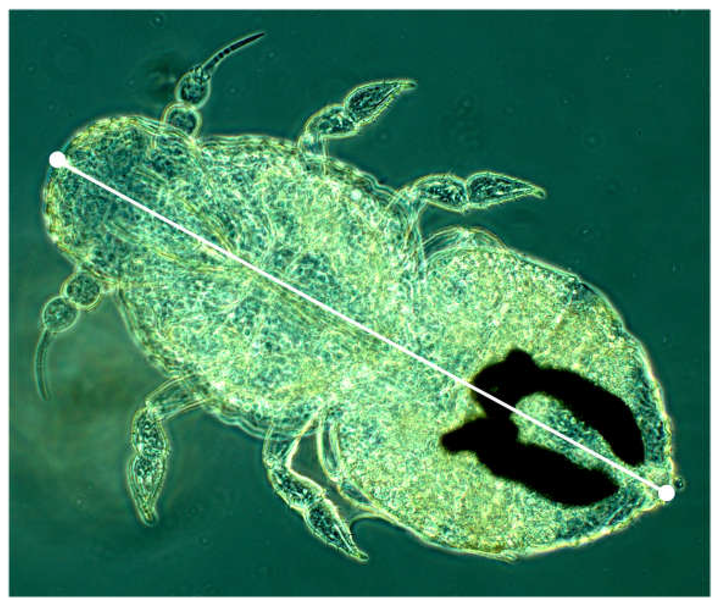
Figure 2.
Distribution of total body length within the clusters and affiliation to the five Homogeneous Groups of the Multiple Range Test for mean comparison, which were shown to correspond to the instars.
Figure 2.
Distribution of total body length within the clusters and affiliation to the five Homogeneous Groups of the Multiple Range Test for mean comparison, which were shown to correspond to the instars.
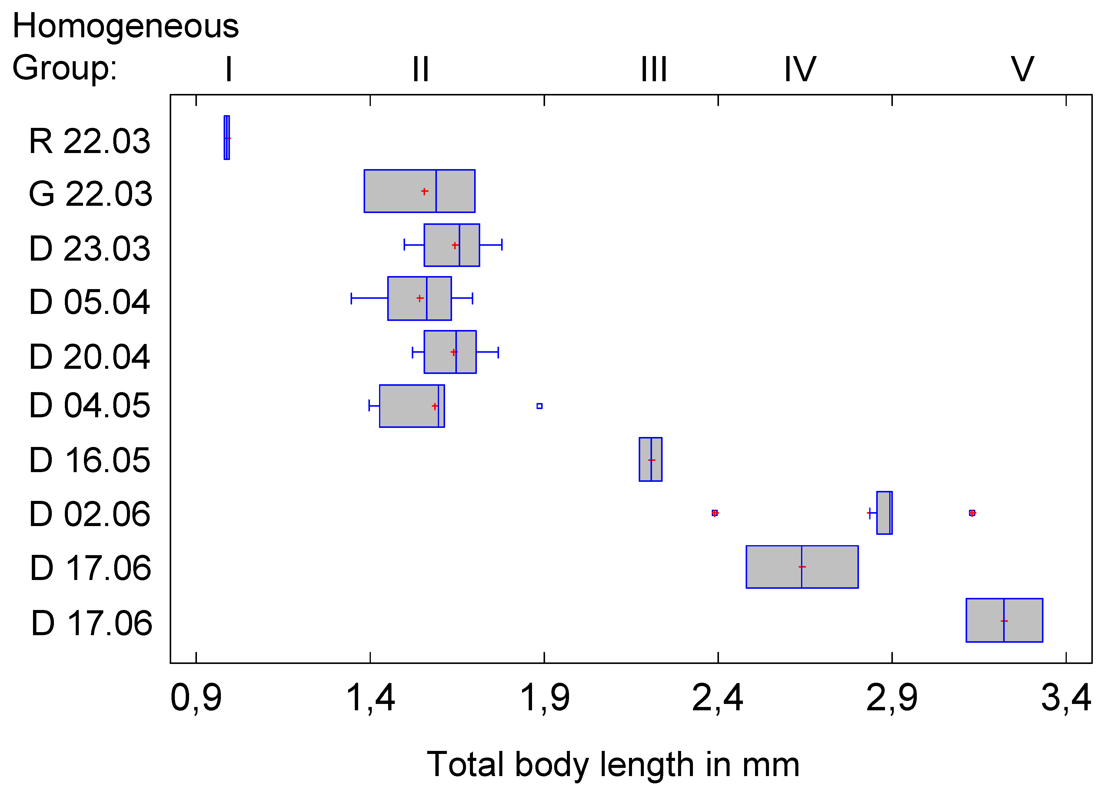
Figure 3.
Body length of the instars (or the Homogeneous Groups of the statistical analysis). Note that the intersegmental integuments are less sclerotised and therefore the length of the abdomen in particular may depend on the preparation.
Figure 3.
Body length of the instars (or the Homogeneous Groups of the statistical analysis). Note that the intersegmental integuments are less sclerotised and therefore the length of the abdomen in particular may depend on the preparation.
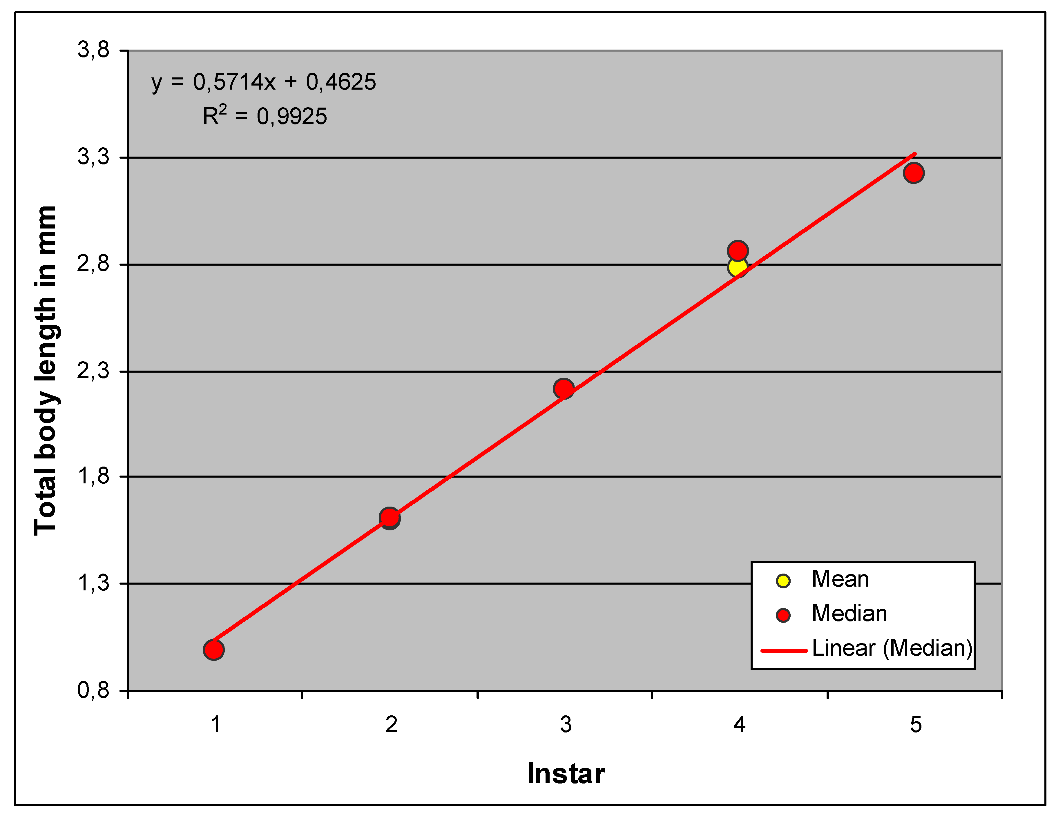
Figure 4.
Measurement of the antenna of the first instar (L1).
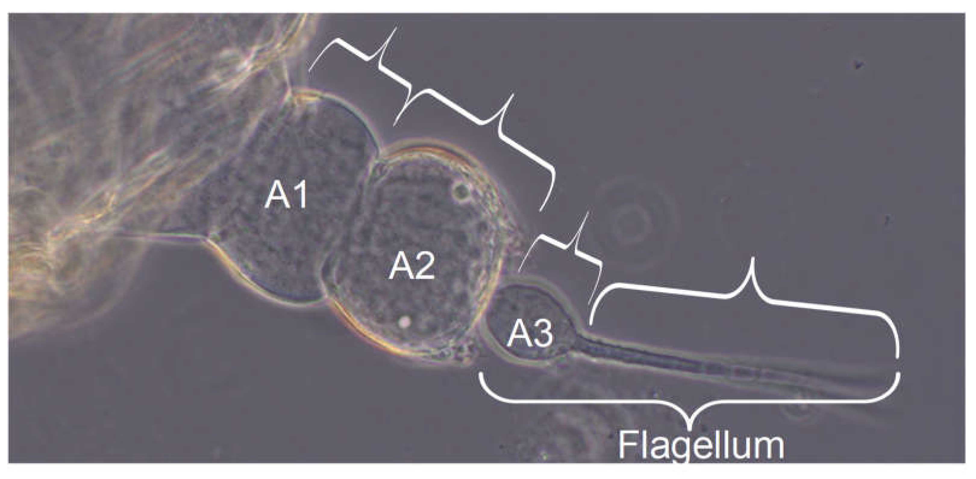
Figure 5.
Distribution of antenna length within the clusters and affiliation to the five Homogeneous Groups of the Multiple Range Test.
Figure 5.
Distribution of antenna length within the clusters and affiliation to the five Homogeneous Groups of the Multiple Range Test.
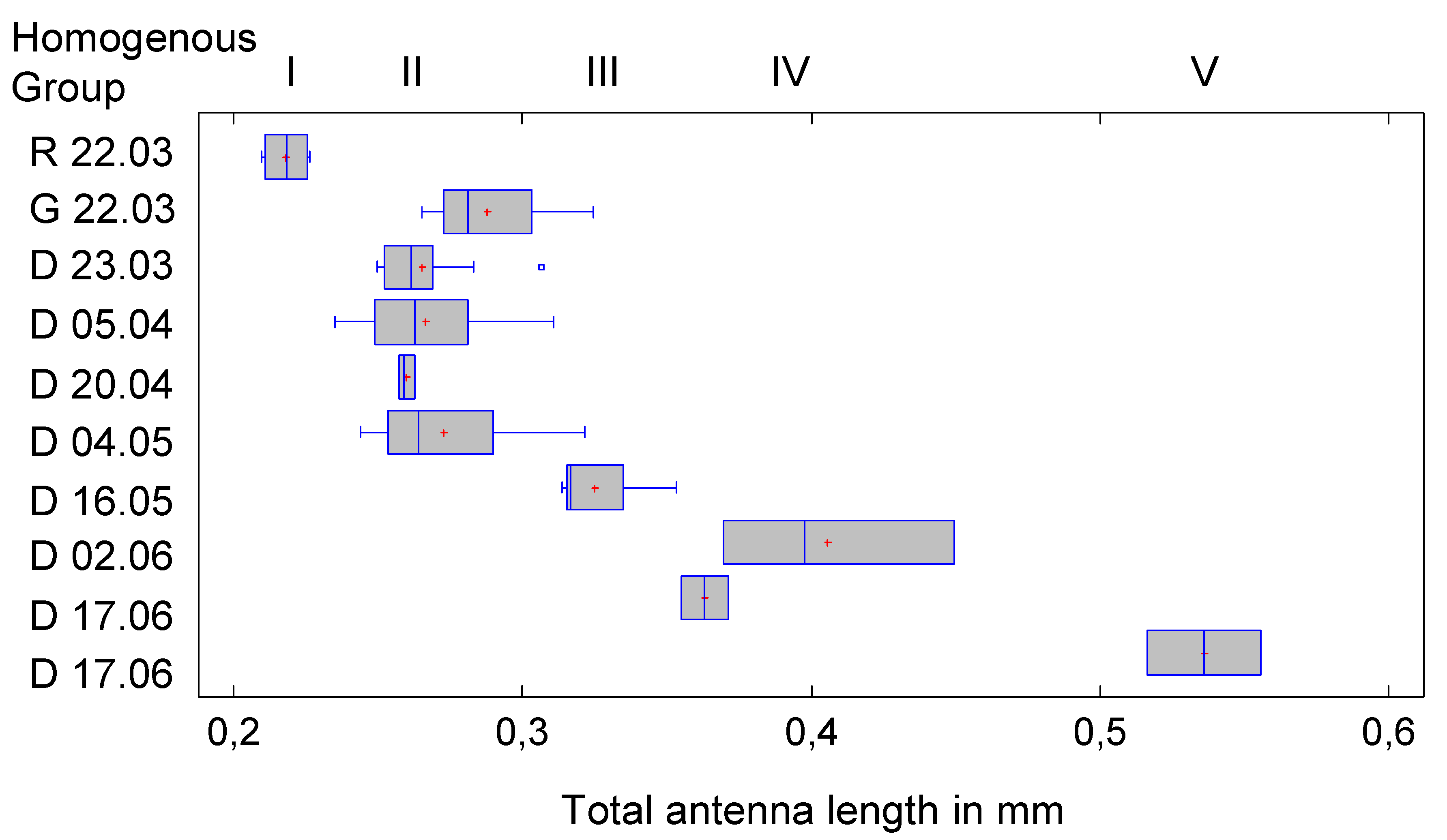
Figure 6.
Comparison of antennal length in the instars (the Homogeneous Groups of the statistical analysis).
Figure 6.
Comparison of antennal length in the instars (the Homogeneous Groups of the statistical analysis).
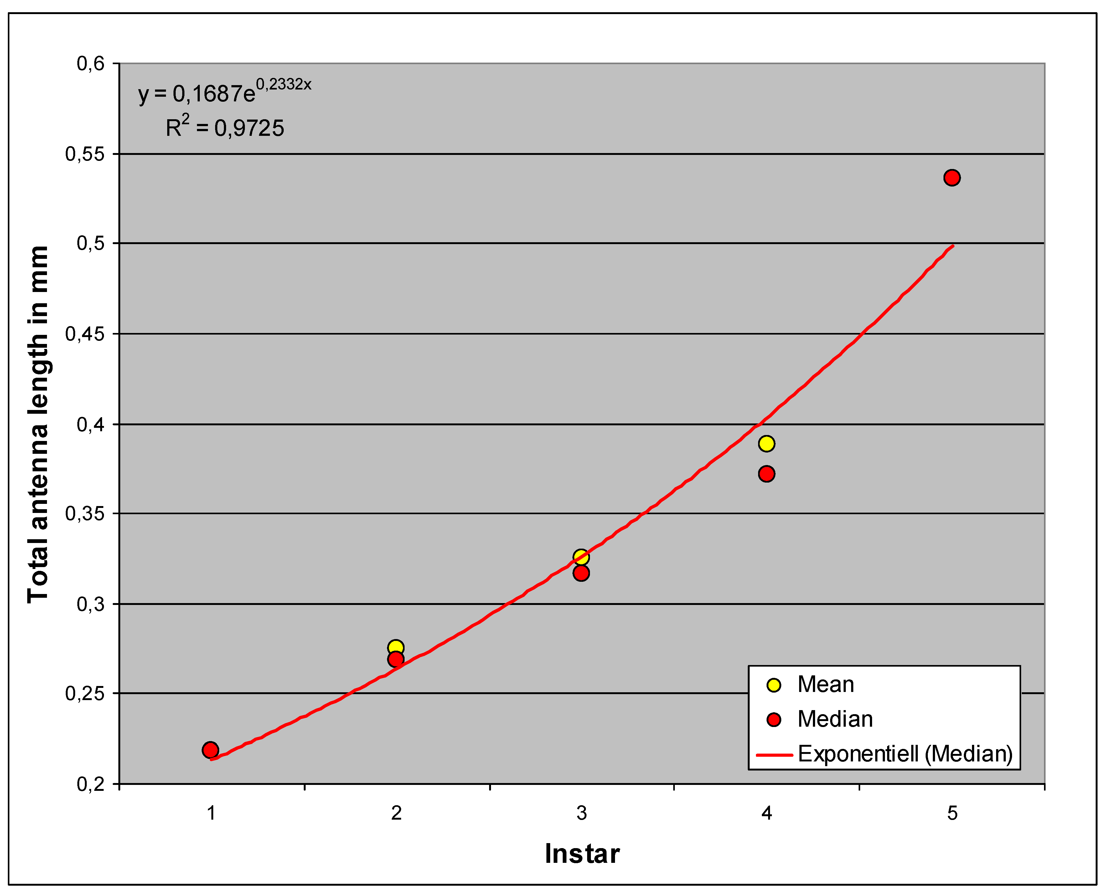
Figure 7.
The labium, consisting of submentum, mentum and postmentum (L1).
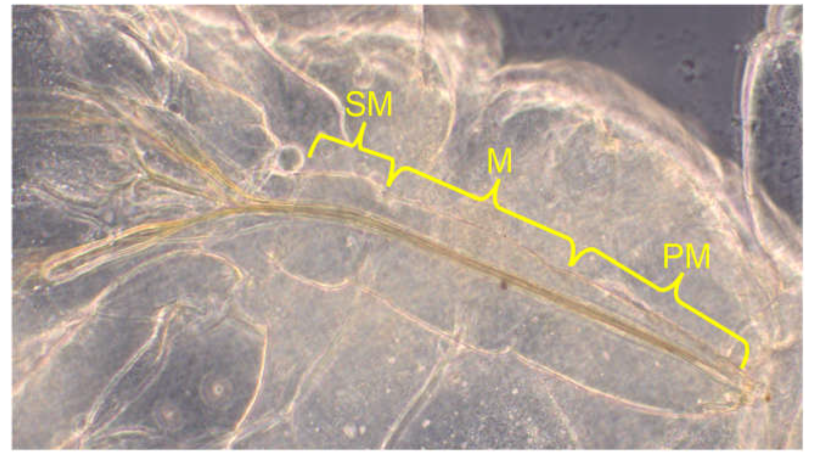
Figure 8.
Distribution of labium length within the clusters and affiliation to the five Homogeneous Groups of the Multiple Range Test.
Figure 8.
Distribution of labium length within the clusters and affiliation to the five Homogeneous Groups of the Multiple Range Test.
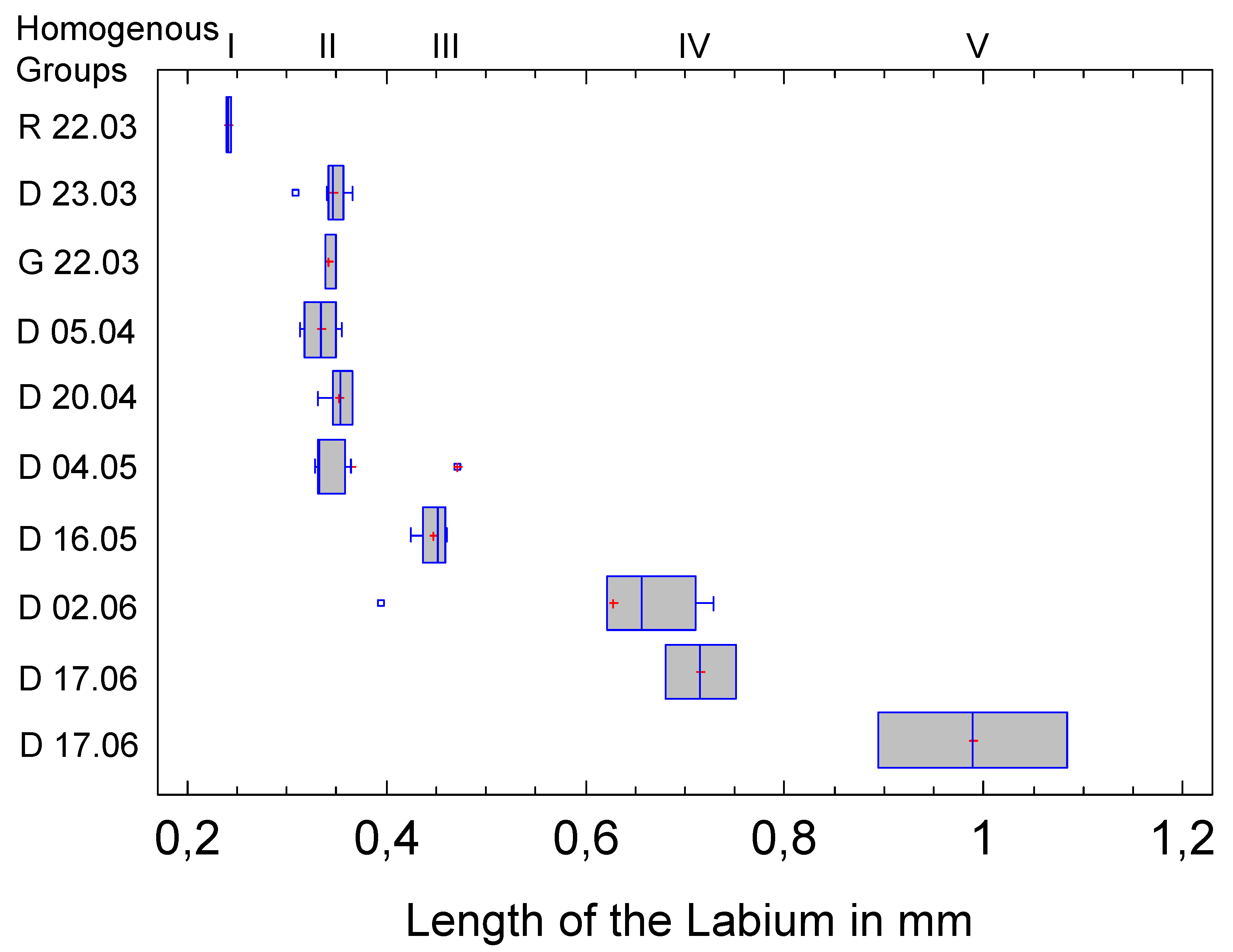
Figure 11.
Distribution of hind limb length within the clusters and affiliation to the five instars (Homogeneous Groups of the Multiple Range Test).
Figure 11.
Distribution of hind limb length within the clusters and affiliation to the five instars (Homogeneous Groups of the Multiple Range Test).
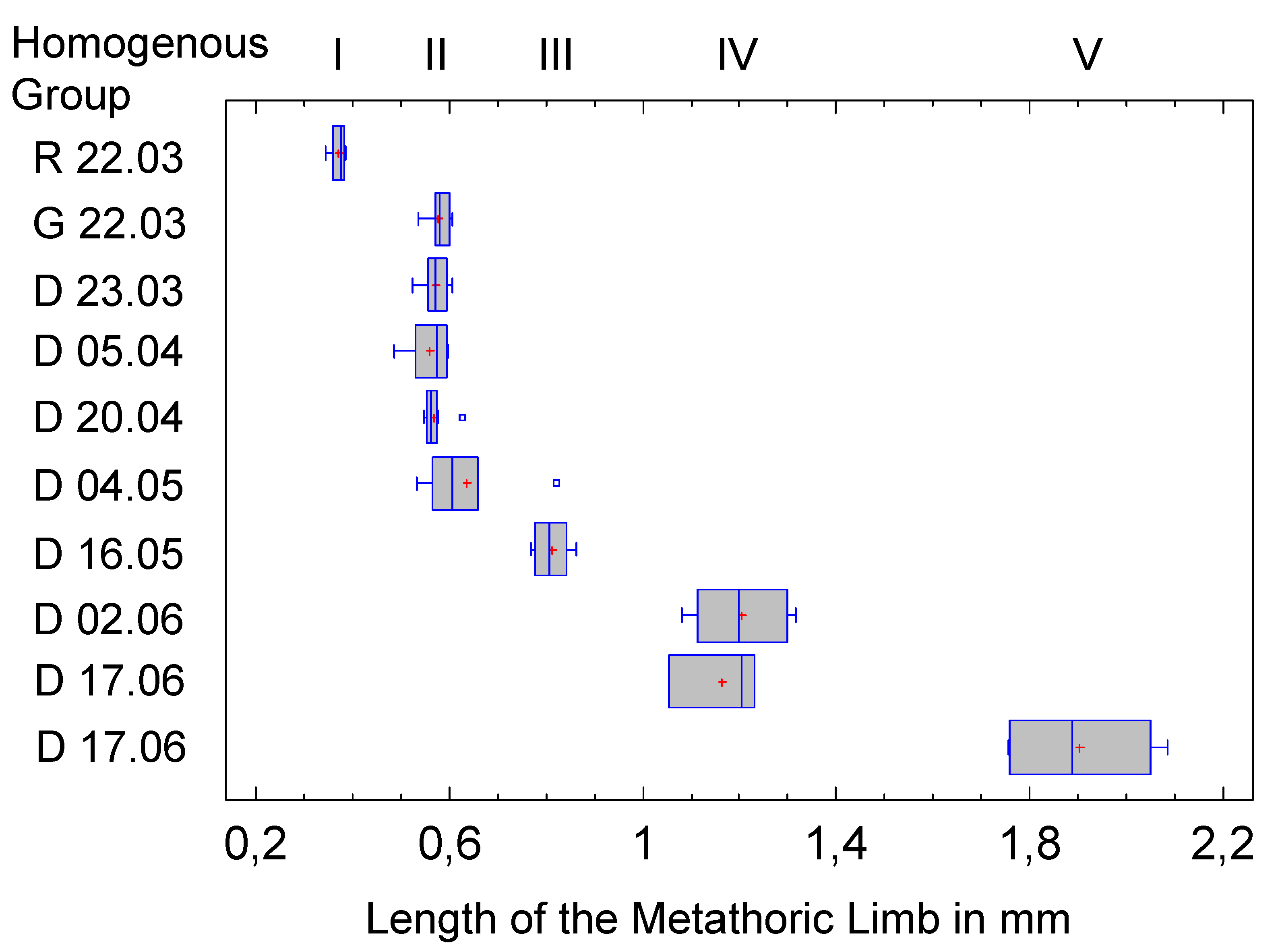
Figure 12.
Comparison of the length of the hind limbs in the instars ( Homogeneous Groups of the statistical analysis).
Figure 12.
Comparison of the length of the hind limbs in the instars ( Homogeneous Groups of the statistical analysis).
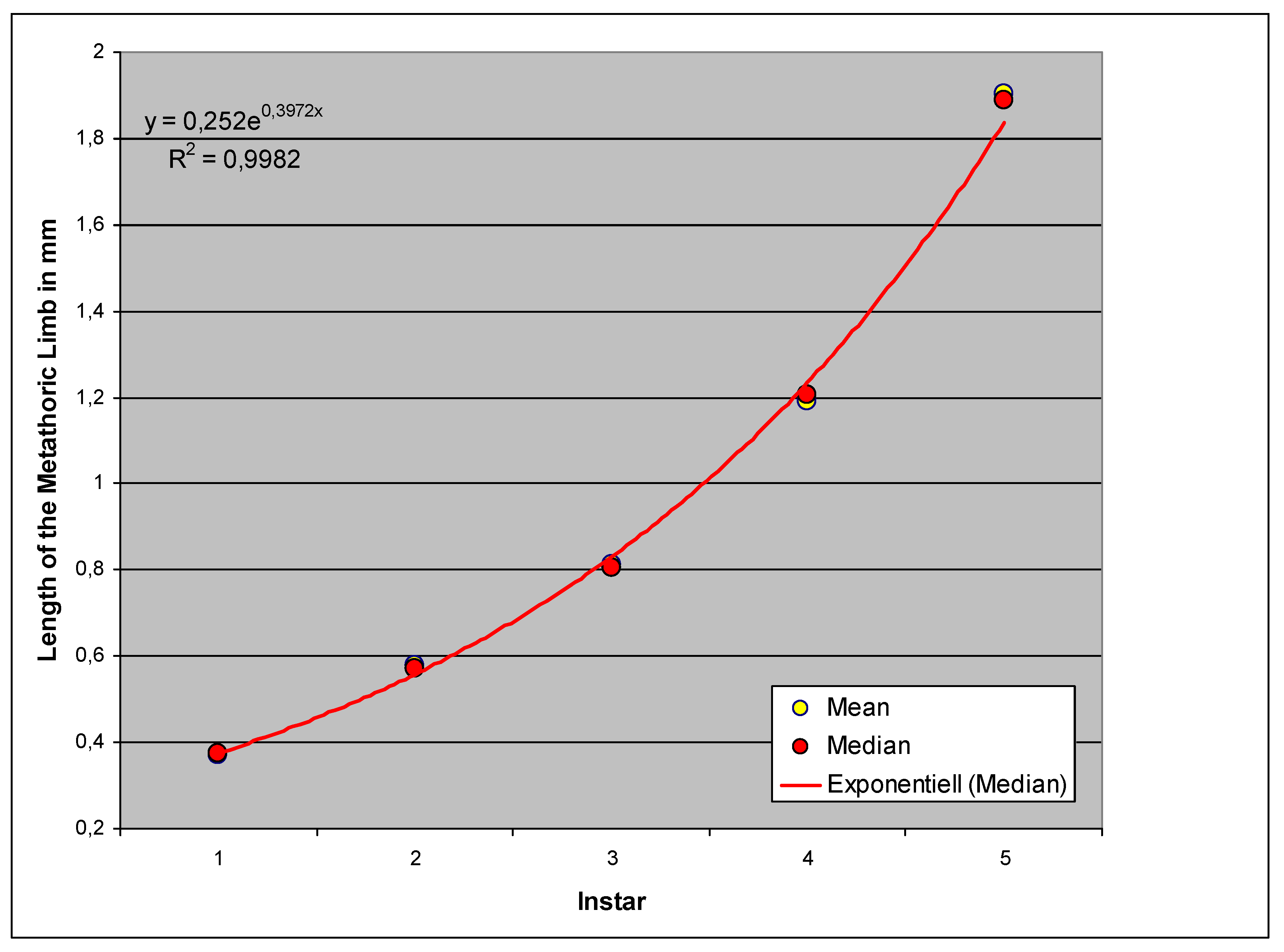
Figure 13.
Comparison of the exponents of the fitting curves describing the growth of the features during larval development.
Figure 13.
Comparison of the exponents of the fitting curves describing the growth of the features during larval development.
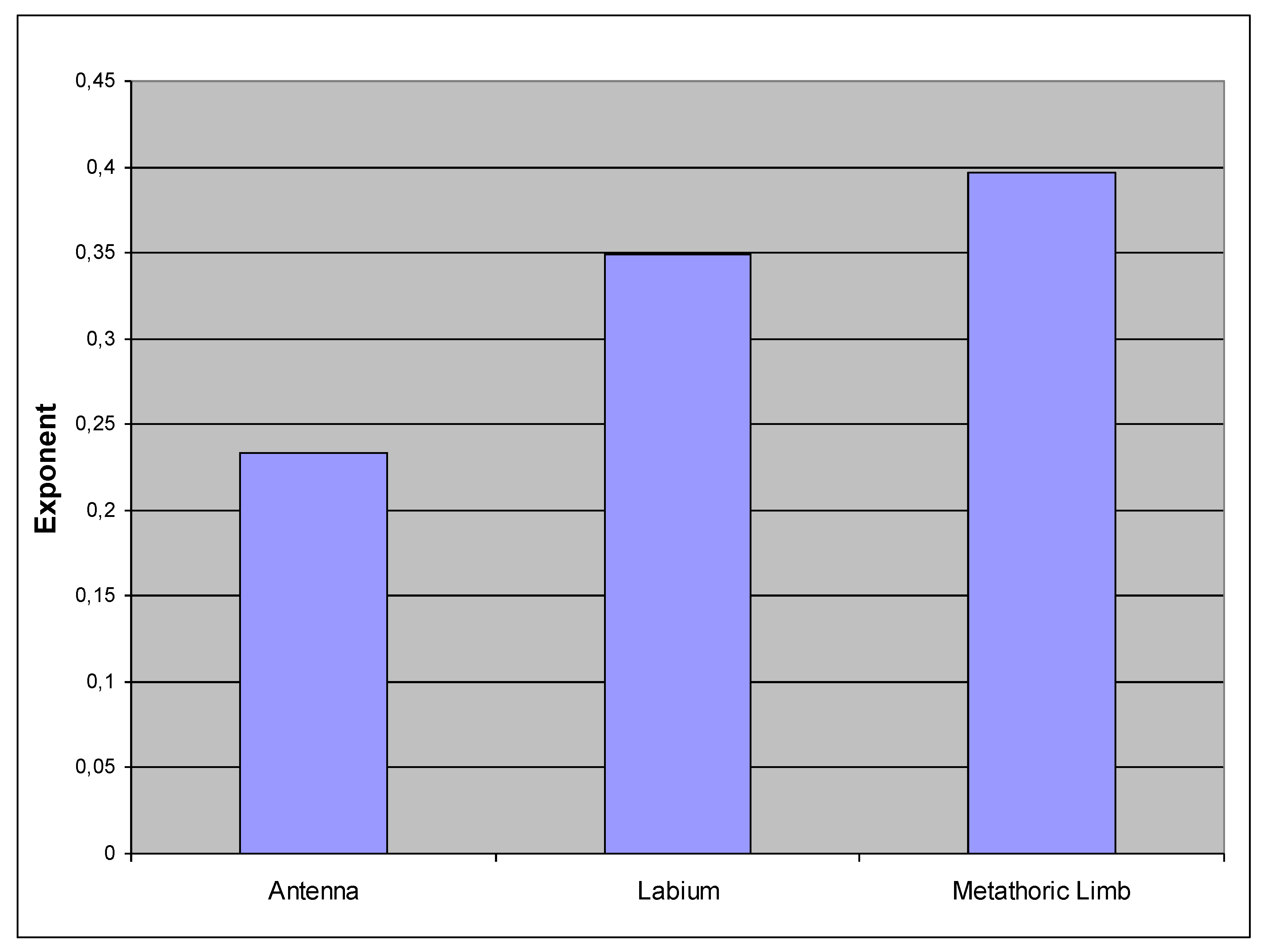
Figure 14.
Principal Component Analysis (left) for eleven body features (right) and 87 objects (individuals or bilateral body sides).
Figure 14.
Principal Component Analysis (left) for eleven body features (right) and 87 objects (individuals or bilateral body sides).
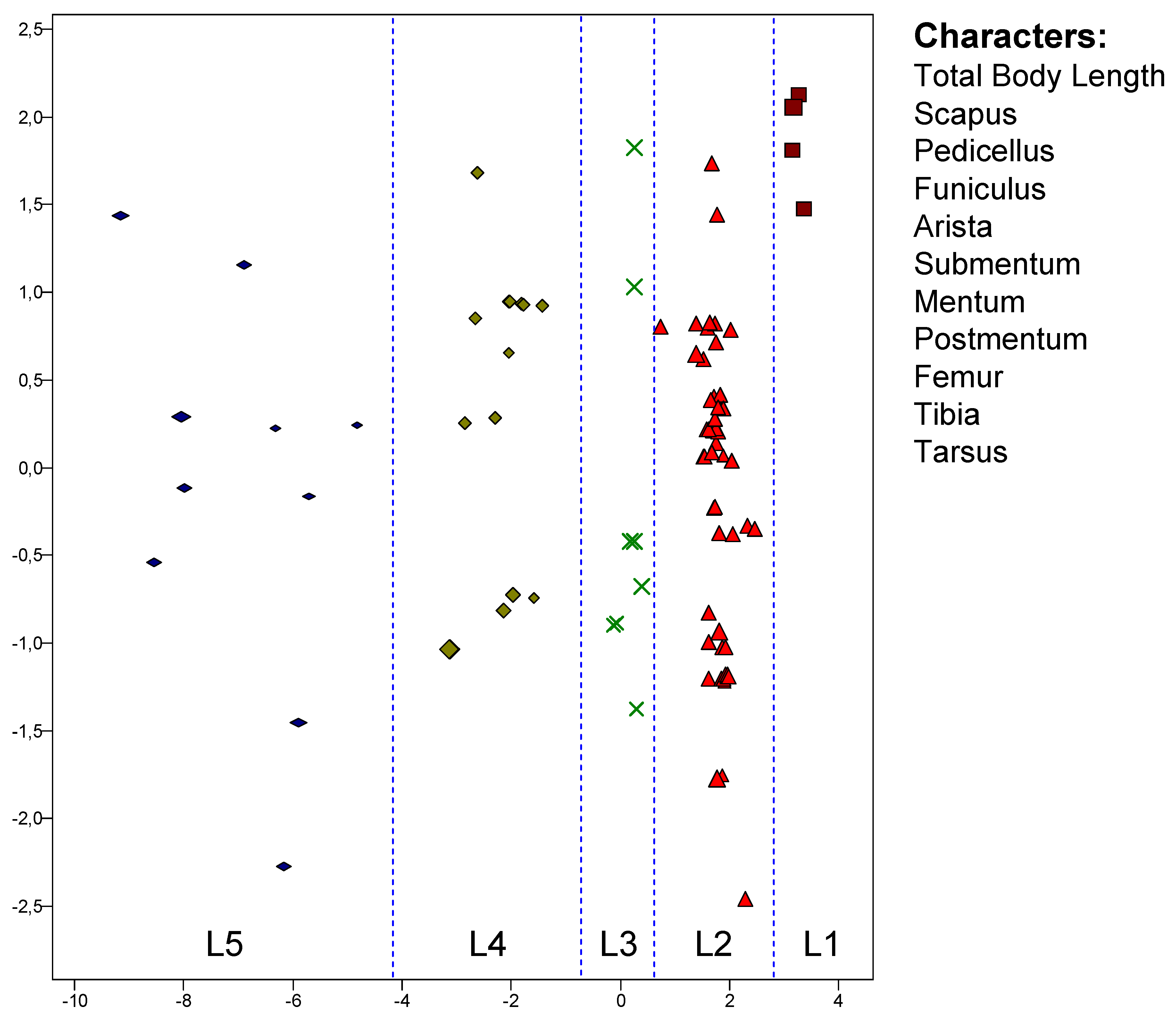
Figure 15.
Antenna of the second instar (L2). The flagellum is divided into the basal, bulbous funiculus, on which the arista and a candle-shaped extension called spur are inserted.
Figure 15.
Antenna of the second instar (L2). The flagellum is divided into the basal, bulbous funiculus, on which the arista and a candle-shaped extension called spur are inserted.
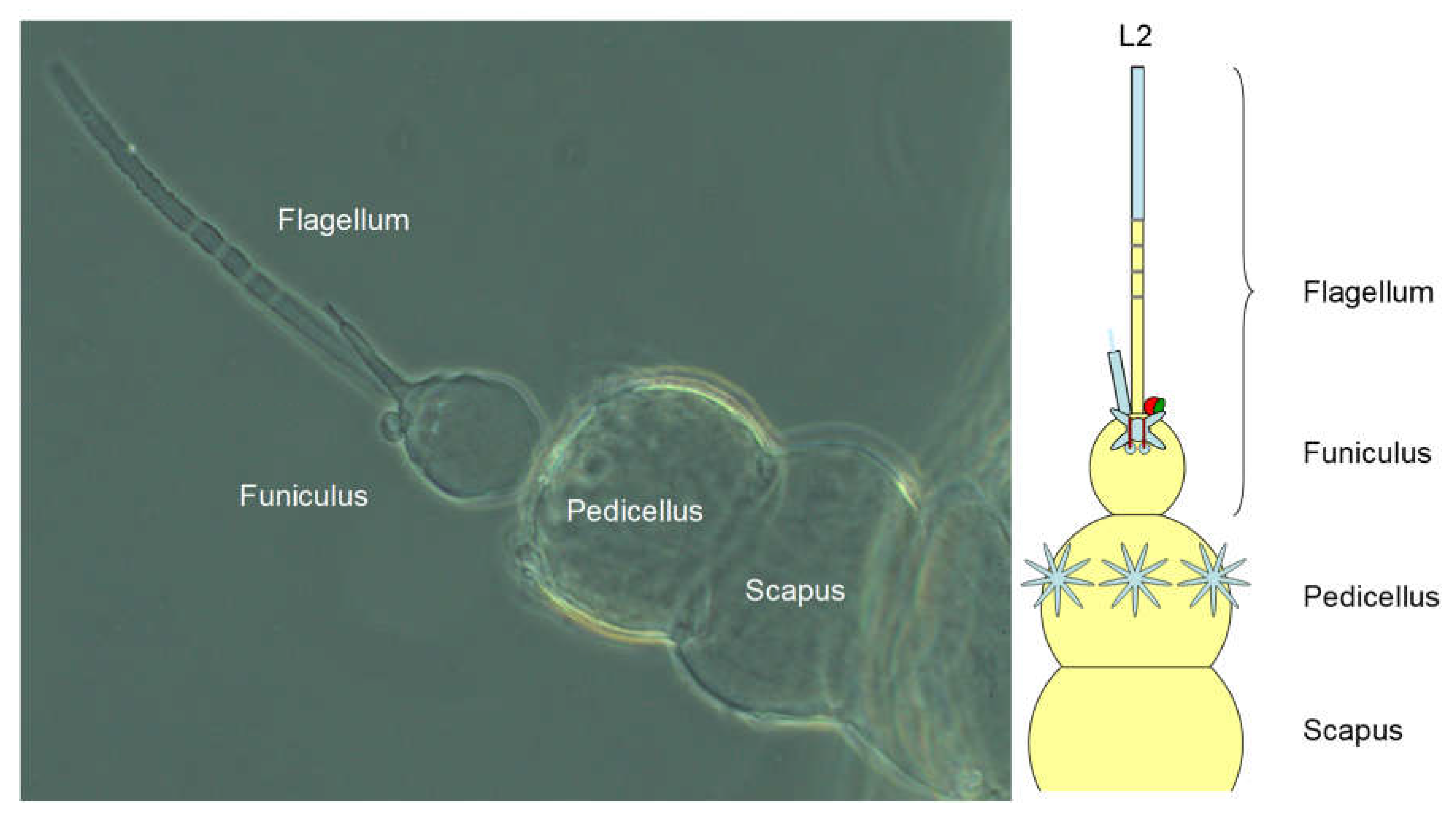
Figure 16.
Sensors and sensor areas of the antennas. For alternative designations of the sensors, see main text. The schematic representations of the sensors are used in Figure 17.
Figure 16.
Sensors and sensor areas of the antennas. For alternative designations of the sensors, see main text. The schematic representations of the sensors are used in Figure 17.
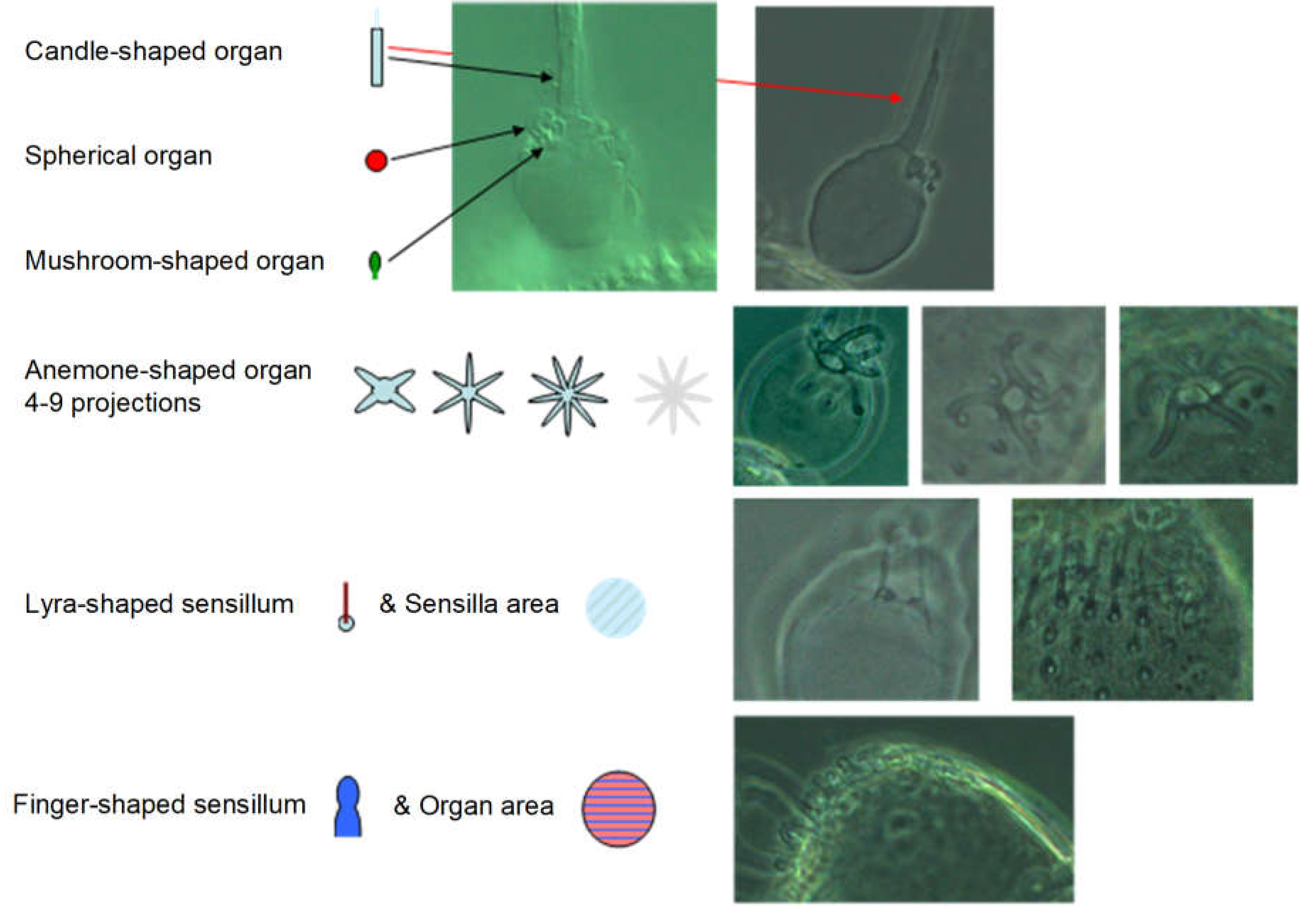
Figure 19.
Median and lateral stripes for coding the trichobothria pattern on the pro-, meso- and metanotum.
Figure 19.
Median and lateral stripes for coding the trichobothria pattern on the pro-, meso- and metanotum.
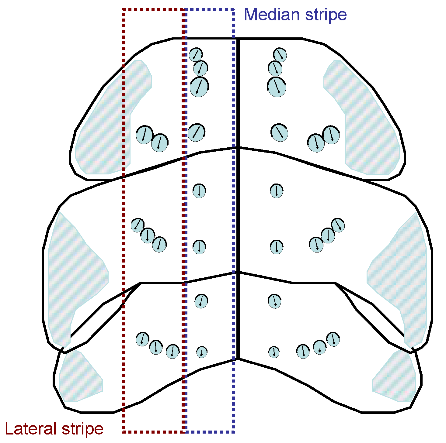
Figure 20.
Trichobothria pattern on the thoracic dorsum in the different instars.
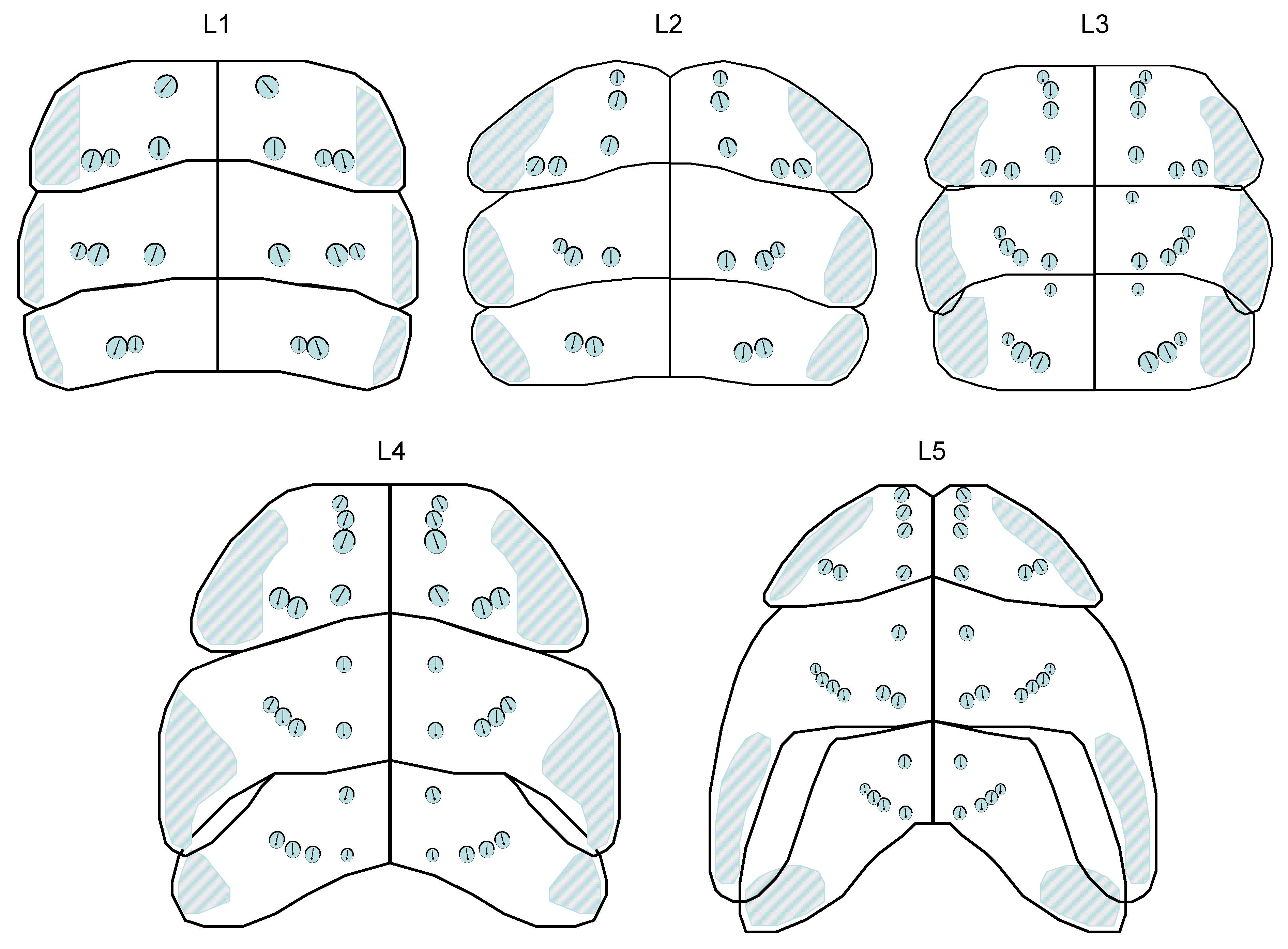
Figure 21.
Gear-like trochanter formation (“gear-teeth”) in the hind leg, which is intended to synchronize movement when jumping.
Figure 21.
Gear-like trochanter formation (“gear-teeth”) in the hind leg, which is intended to synchronize movement when jumping.
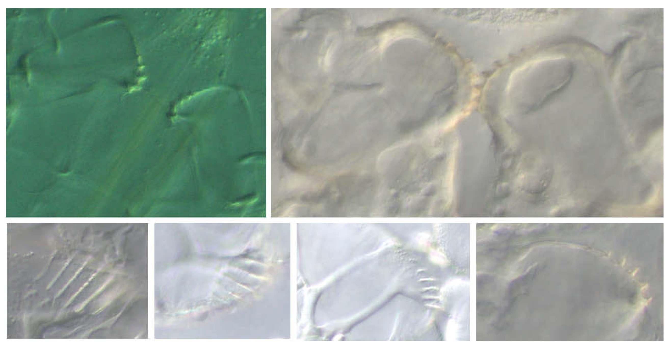
Figure 22.
Jumping leg of the second instar with a comparison of trichium (top right) and apical bristle (bottom right).
Figure 22.
Jumping leg of the second instar with a comparison of trichium (top right) and apical bristle (bottom right).
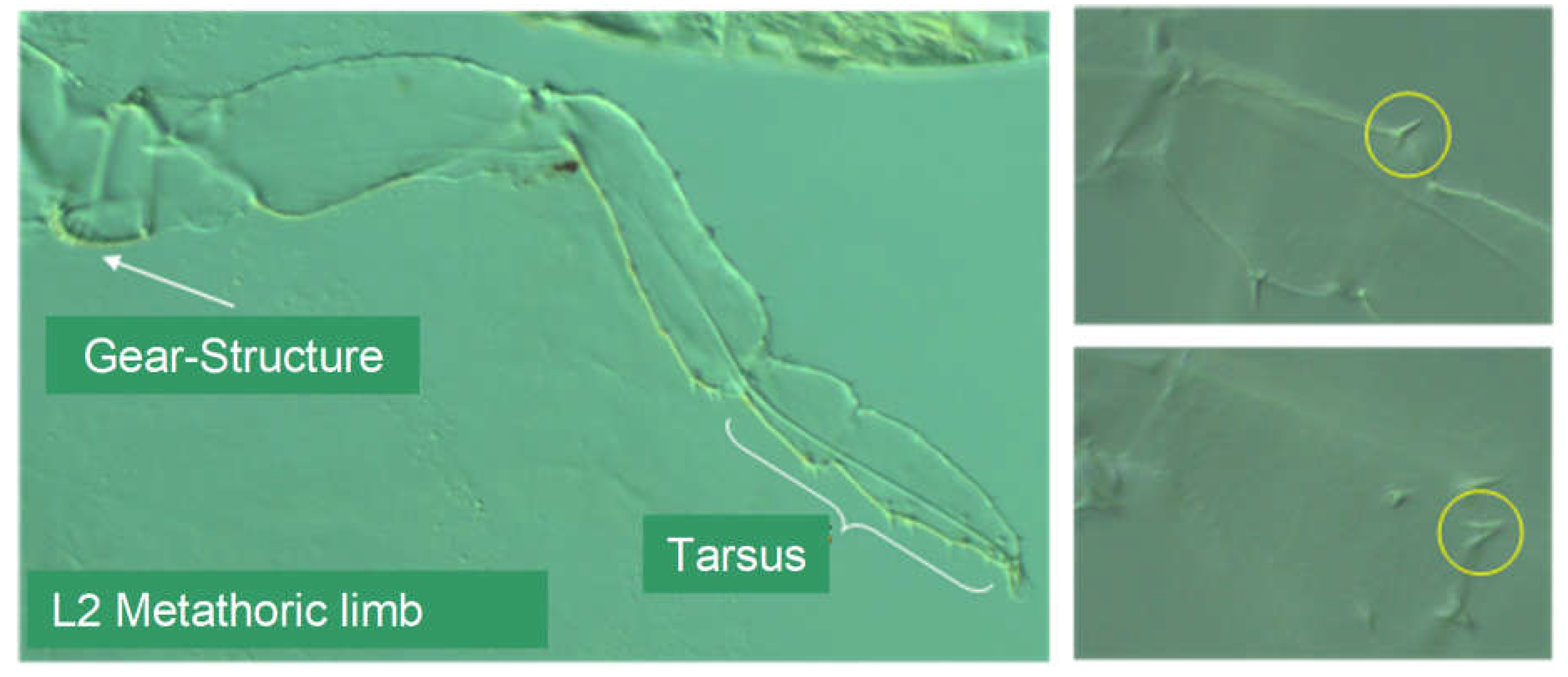
Figure 23.
Tarsus of the hind leg in different instars.
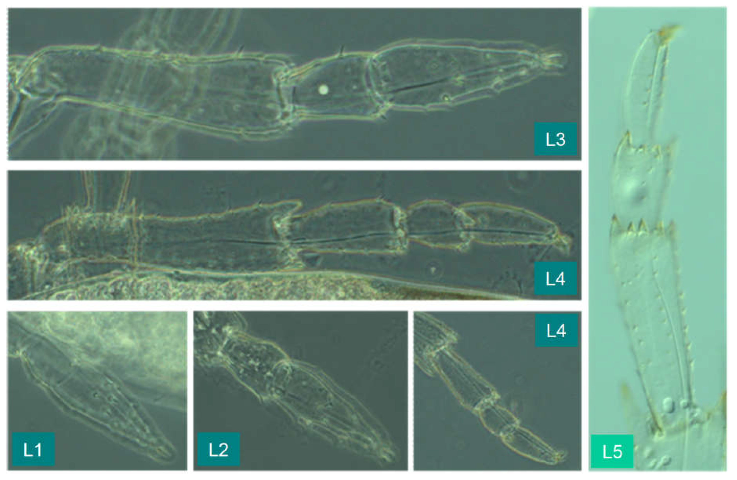
Figure 24.
Schematic representation of the hind leg tarsus. A verbal description can be found in the main text.
Figure 24.
Schematic representation of the hind leg tarsus. A verbal description can be found in the main text.
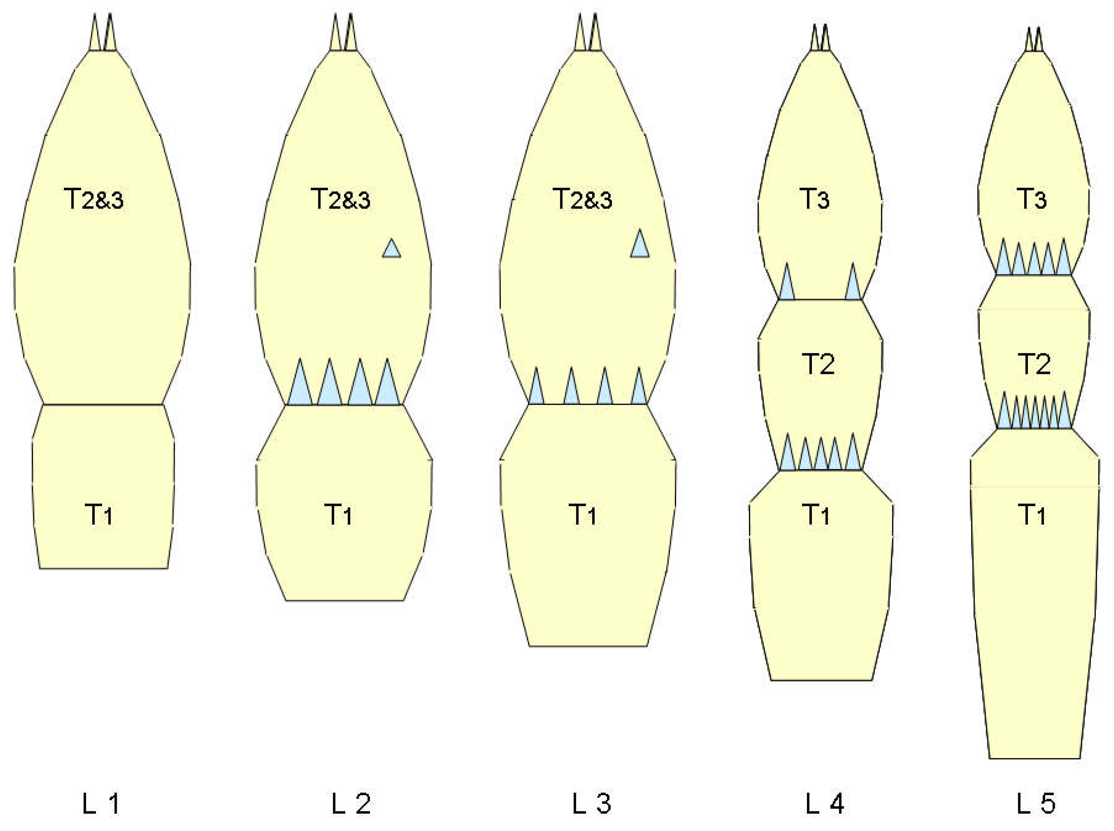
Figure 25.
Schematic representation of the wax plates of tergites VI to VIII of the abdomen.
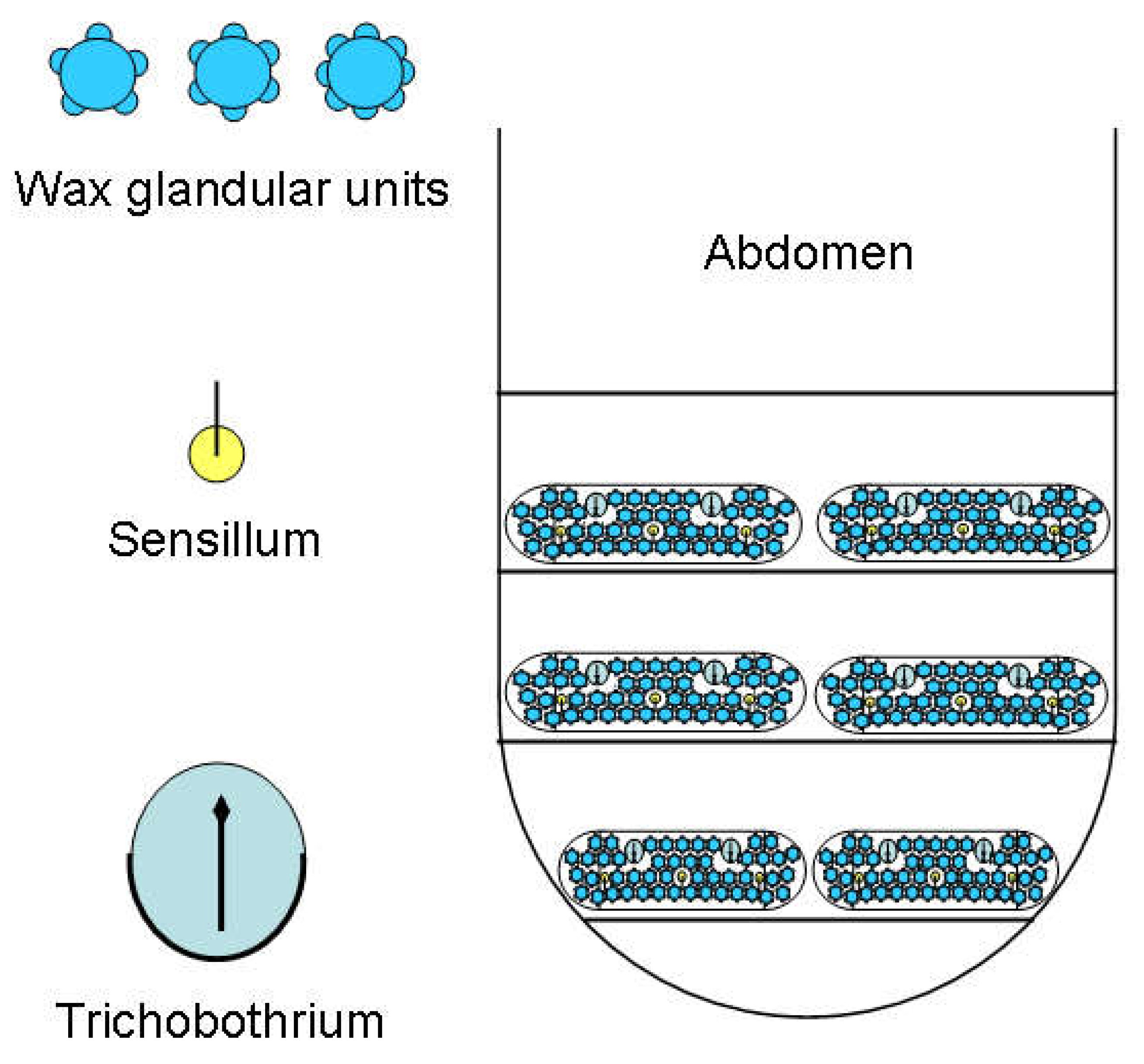
Figure 26.
Wax plate of L1. Comparison of the diagrams with the photograph (phase and interference contrast).
Figure 26.
Wax plate of L1. Comparison of the diagrams with the photograph (phase and interference contrast).
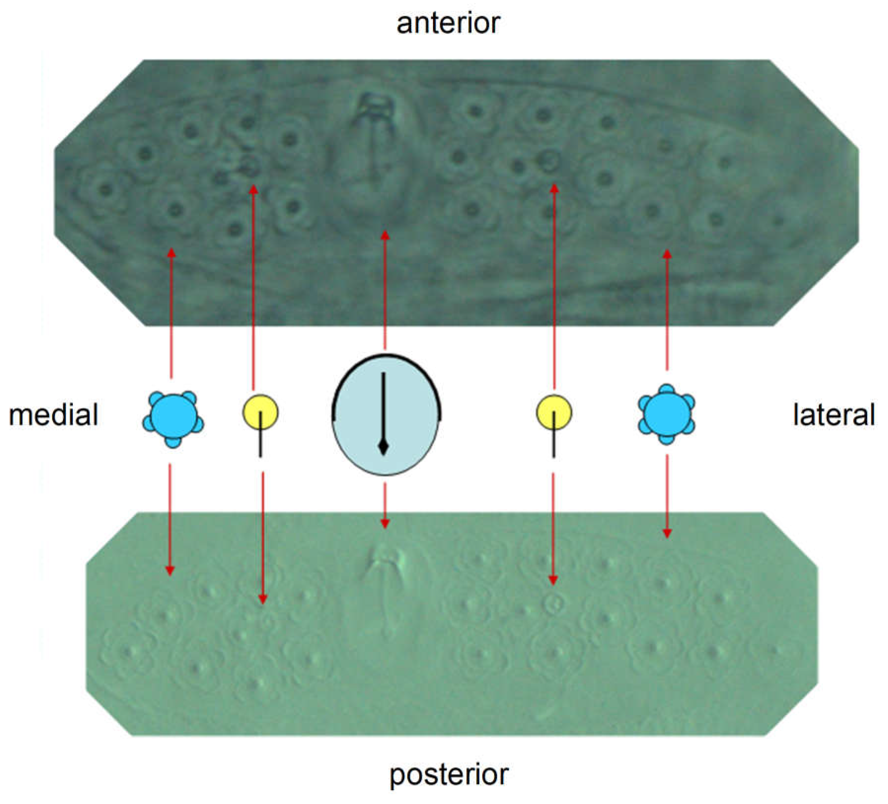
Figure 27.
Schematic representation of the wax plates for all instars.
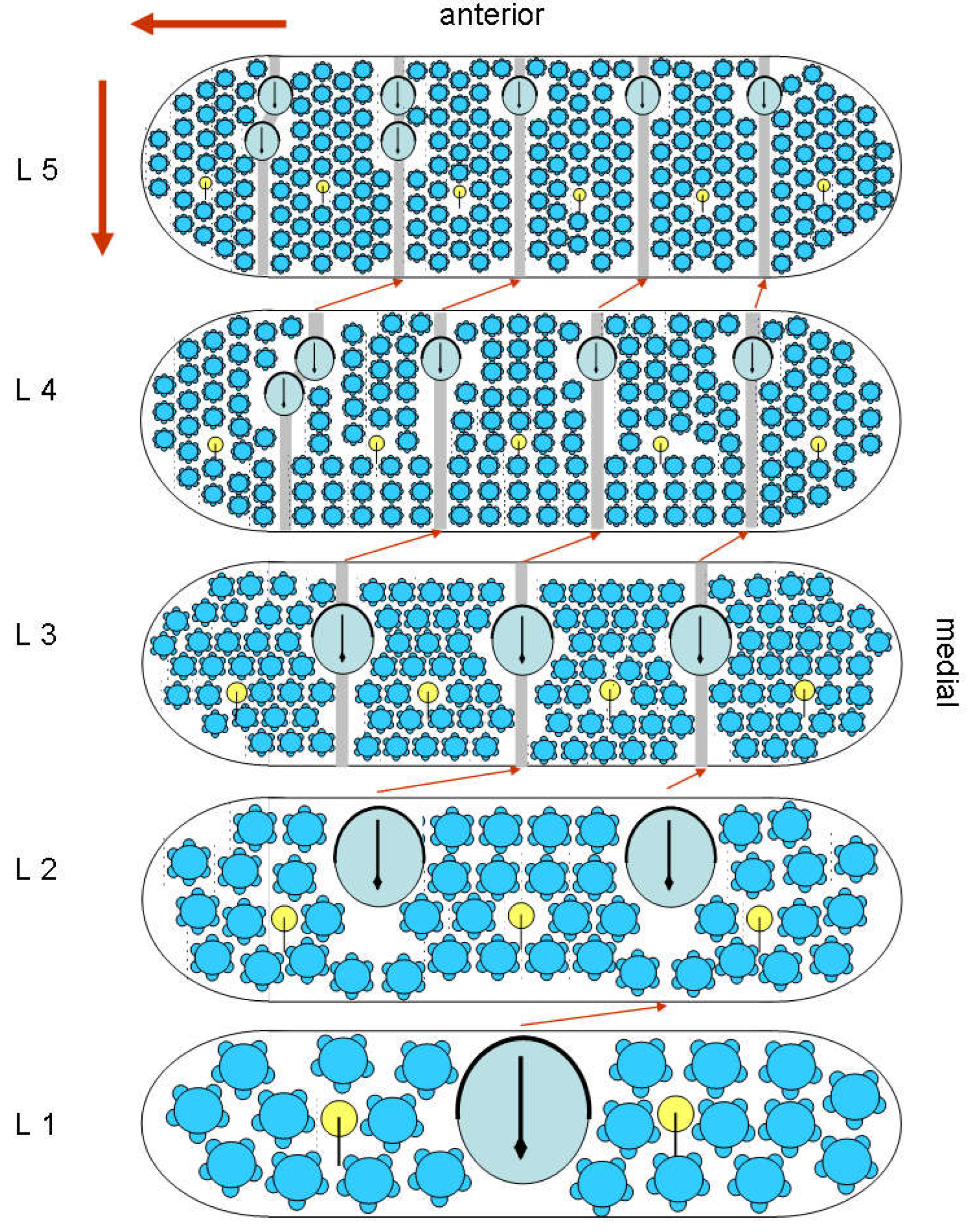
Figure 28.
Photographs of the wax gland plates in instars L2 (a,b), L3 (c), und L4 (e,f).
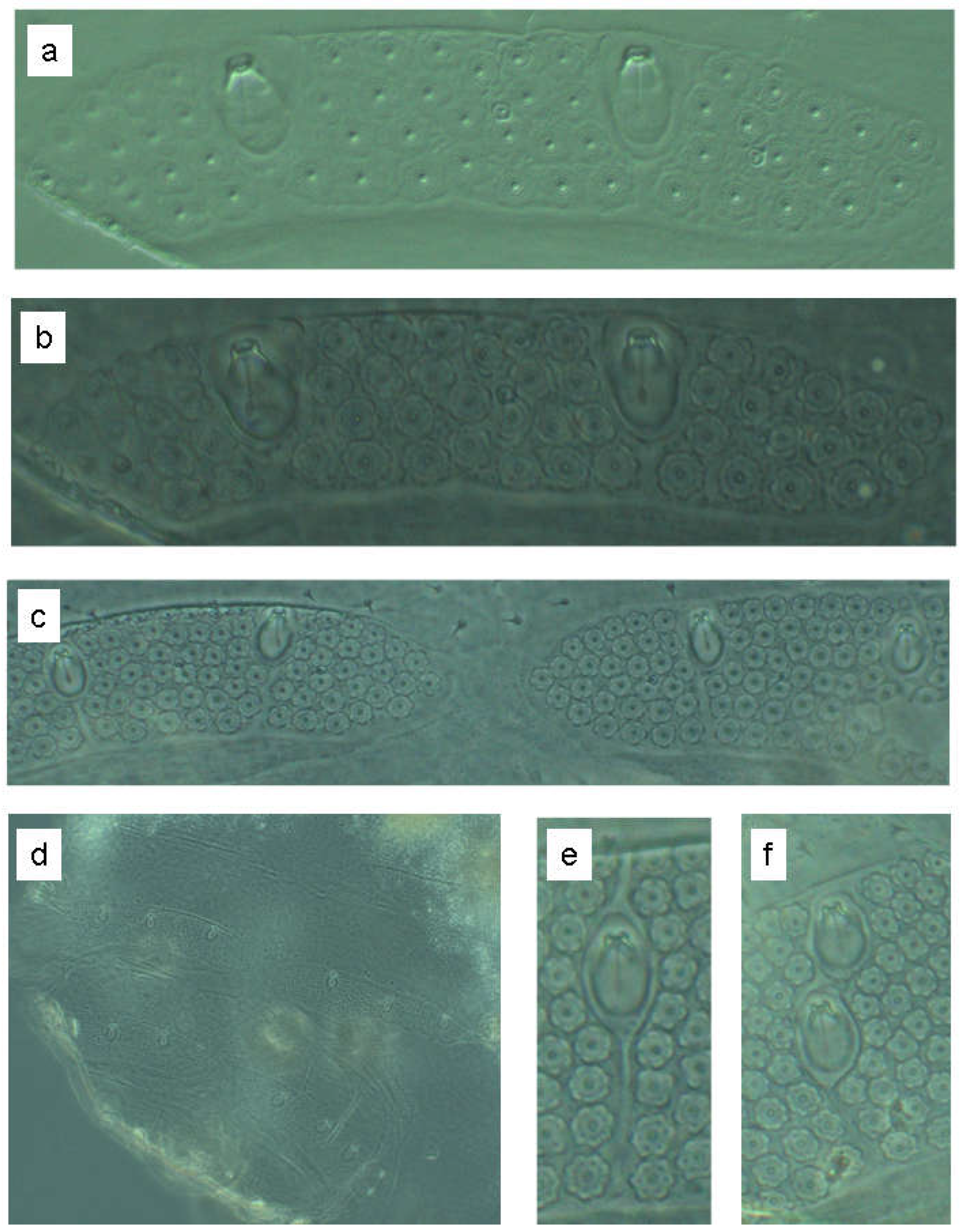
Table 1.
Body length of the larvae. Comparison of the metric data according to Sforza et al. 1999 with the present results. ‘Count’ indicates the number of individuals per cluster. R: Rust; D: Donnerskirchen-Wolfsbrunnbach; G: Donnerskirchen-Goldberg. D-17.06 was divided into two clusters a and b, as the sample apparently contains two different instars.
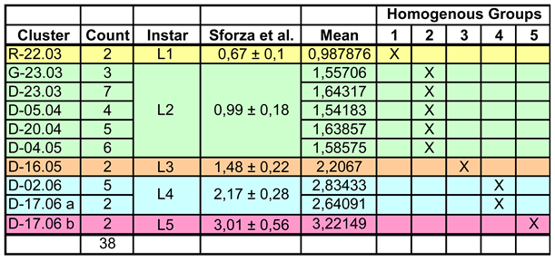 |
Table 5.
Characteristics of the instars L1 – L5.
 |
Disclaimer/Publisher’s Note: The statements, opinions and data contained in all publications are solely those of the individual author(s) and contributor(s) and not of MDPI and/or the editor(s). MDPI and/or the editor(s) disclaim responsibility for any injury to people or property resulting from any ideas, methods, instructions or products referred to in the content. |
© 2025 by the authors. Licensee MDPI, Basel, Switzerland. This article is an open access article distributed under the terms and conditions of the Creative Commons Attribution (CC BY) license (http://creativecommons.org/licenses/by/4.0/).
Copyright: This open access article is published under a Creative Commons CC BY 4.0 license, which permit the free download, distribution, and reuse, provided that the author and preprint are cited in any reuse.


