1. Introduction
Retinopathy and Glaucoma are diseases that primarily affect the population of Mexico, “in Mexico it is estimated that there are about 1.5 million with Glaucoma, and up to 50 thousand cases of blindness due to its late detection.” [
1]
Eye diseases such as Diabetic Retinopathy and Glaucoma must be differentiated from the healthy eye to have early detection and thus receive adequate treatment to reduce their progress and effects. These diseases have been a severe problem worldwide, specifically in underdeveloped countries that do not have enough technology or economy to treat them. Today, the problem has been solved thanks to certain pattern recognitions, which aim to highlight specific characteristics of any object, phenomenon, or event that belongs to the real world.
1.1 Eye diseases
Glaucoma [
2] is the term used to define the increase in intraocular pressure, which causes alteration of the optic nerve. The etiopathogenesis of Glaucoma lies in the difficulty in the exit of aqueous humor through the trabeculum, and the treatment is focused on reducing the production of aqueous humor and facilitating its exit. The presence of Glaucoma is one of the reasons for vision loss, which spreads through the eye.
There are at least four types of Glaucoma:
1. Primary open-angle Glaucoma
2. Primary angle-closure Glaucoma
3. Secondary glaucoma
4. Normal-Tension Glaucoma
Diabetic Retinopathy [
3] occurs because high blood sugar levels cause damage to the blood vessels in the retina. These blood vessels can swell and leak fluid and even close and prevent blood from flowing. Sometimes, it generates new abnormal blood vessels in the retina, causing vision loss.
There are three types of Diabetic Retinopathy[
4]:
1. Non-Proliferated Diabetic Retinopathy.
2. Proliferative Diabetic Retinopathy (PDR), where a distinction is made between blood leaks or occlusions and their position in the eye.
3. Diabetic Vasculopathy.
Cataract
A cataract [
5] is when the natural lens of the eye becomes cloudy. Proteins in your lens break down and make things look blurry, fuzzy, or less colorful.
Here are some vision changes that can be noticed if there is a cataract: Blurry vision, seeing double or ghosting through the eye with cataracts, high sensitivity to light, difficulty seeing well at night or needing more light to read or seeing bright colors dimmed or yellowed.
1.2 Related work
Dheeraj and Ghosh [
6] classified six ocular diseases: age-related macular degeneration, cataracts, diabetes, glaucoma, hypertension, and myopia. They applied a Vision Transformer-based approach with three different architectures with 8, 14, and 24 layers. The architecture with 14 layers obtained the best results with F1-score of 83.49%, 84% sensitivity, 83% precision, and 0.802 Kappa score. They used the ODIR dataset, trained and validated the algorithms with 80% of the dataset, and used the 20% for testing.
Wahab [
7] built a deep learning-based eye disease classification model. Three steps are applied; the first is detecting main features using the Single-Shot detection algorithm. Then, the whale optimization algorithm (WOA) with Levy Flight and Wavelet search strategy is applied for feature selection, and finally, the ShuffleNet V2 model is used for image classification. Eight classes are analyzed: normal, DR, glaucoma, cataracts, age-related macular degeneration, hypertension, pathological myopia, and other diseases/abnormalities. Two data sets are used: the ocular disease intelligent recognition (ODIR) dataset and the EDC dataset that was used to train the ShuffleNet V2 model. Both datasets were obtained from the Kaggle platform. The dataset was split into two parts: 70% for training and 30% for testing. The metrics and their corresponding results are: Accuracy = 99.1%, Precision = 98.9%, Recall = 99%, F1 – Score = 98.9%, Kappa = 96.4%, Sensitivity = 98.9% and Specificity = 96.3%.
In 2023 [
8], the authors applied three deep learning-based approaches: the EfficientNetB0, VGG-16, and VGG-19 models. The dataset was obtained from the Kaggle platform, which contains images of four eye diseases: Normal, Diabetic Retinopathy, Cataract, and Glaucoma. The dataset was split into two parts: training and testing, 70% and 30%, respectively. The metrics used to measure the performance of the classification models were Accuracy, Precision, Recall, and AUC. The algorithm that obtained the best results was EfficientNetB0: Accuracy = 98.47%, Precision = 96.98%, Recall = 96.91%, and AUC = 99.84%.
Mostafa
et al. [
9] used a Convolutional Neural Network with a pre-processing of normalization and CLAHE algorithm. They analyzed six distinct diseases, including glaucoma, cataract, diabetes, age-related macular degeneration, hypertension, pathological myopia, and other diseases not explicitly mentioned in the Ophthalmic Disease Recognition (ODIR) dataset. The dataset was split into two groups for 70% training and 30% validation. The authors applied a data augmentation algorithm to balance the classes. The metrics used to measure the performance of the classification models were Accuracy, Precision, Recall, and AUC. Two experiments were developed; the first consisted of classifying all the diseases together (multiclass classification), and in the second, each of the diseases was taken and classified together with the normal class (binary classification). In the first experiment, they obtained an accuracy of 60.31% and an AUC of 85%. For the second experiment, the accuracy was between 98% and 100%, recall from 97.99% to 100%, and precision between 96% and 100%.
Two classification models were used to detect eye diseases: a Convolutional Neural Network and a pre-trained model, EfficientNet CNN [
10]. The diseases to be classified are Cataract, Diabetic retinopathy, Glaucoma, and Normal. The complete dataset combines four other sets with around 4200 colored images. The data was split into three subsets: 70% training, 20% testing, and 10% validation. Four metrics were applied: Precision, Recall, F1-score, and Accuracy. The best accuracy was obtained with the EfficientNet CNN with 94%.
Elkholy and Marzouk [
11] used a pre-trained Convolutional Neural Network with fine-tuning to detect three eye diseases by analyzing retinal images. They used the images from the dataset Optical Coherence Tomography (OCT). The dataset is balanced. The four classes are Normal retina, Diabetic Macular Edema (DME), Choroidal Neovascular Membranes (CNM), and Age-related Macular Degeneration (AMD). All classes have 8,867 images. The images are pre-processed, enhanced, and restored. These images are fed to a VGG-16 Convolutional Neural Network that classifies the eye diseases. The model accuracy was about 94%, and after fine-tuning, it reached 97%.
A Convolutional Neural Network is implemented to classify three types of eye diseases: Choroidal neovascularization, Diabetic macular edema, and Drusen [
12]. The dataset is obtained from the Kaggle platform and has four classes: the three types of diseases and normal images. The four classes add 84495 Retinal Optical Coherence Tomography (OCT) images. The dataset is split into three subsets: training (99%), testing (0.97%) and validation (0.03%). Three pre-trained models were applied to extract features: VGG-16, Xception, and MobileNet. A Convolutional Neural Network was used for classification. The CNN has two hidden layers; the first has 516 neurons, and the second has 216 neurons. The MobileNet with CNN ensemble model achieves the highest average accuracy, precision, recall, and f1-score, with an average accuracy of 95.34%.
In the current year, Al-Fahdawi et al. [
13] proposed a Fundus-DeepNet system to classify eight ocular diseases. The fundus images were taken from the OIA-ODIR dataset. The dataset consists of 10,000 fundus images representing eight distinct ocular diseases: normal case, diabetic retinopathy, glaucoma, cataracts, AMD, myopia, hypertension, and other abnormalities. The images had a pre-processing procedure, including circular border cropping, image resizing, contrast enhancement, noise removal, and data augmentation. The left and right fundus images are fed to a backbone network to extract the global features from the pre-processed images. The attention block learns additional high-level feature representations to differentiate lesion portions using the output of the backbone network. The fusion process is implemented two times in the attention block and three times in the SENet block. A Discriminative Restricted Boltzmann Machine performs the task of classification. The Fundus-DeepNet system demonstrated F1-scores, Kappa scores, AUC, and final scores of 88.56 %, 88.92 %, 99.76 %, and 92.41 % in the off-site test set, and 89.13 %, 88.98 %, 99.86 %, and 92.66 % in the on-site test set.
2. Materials and Methods
In this section, the algorithms used for both pre-processing and classification of eye diseases will be described. First, the filters used will be described, and then the architecture of the Convolutional Neural Network that performs the classification task will be shown. The methodology used to carry out the classification will then be presented. The data set, the pre-processing algorithms, and the architecture of the Convolutional Neural Network are described. Finally, the metrics used to evaluate the proposed model are shown.
2.1 Blur filters
Blur filters [
14] are used to soften images or selections and are helpful for retouching. This filter reduces sudden changes in light intensity and, therefore, the contrast of images. The most visible consequence is that it blurs images, making them more blurred. This effect, which may worsen the image, helps eliminate noise.
There are some types of these filters, which are described below.
Box Blur: the filter distorts the input image in the following way: Every pixel x in the output image has a value equal to the average value of the pixel values from the 3 × 3 square that has its center at x, and the value of x is included. Finally, all the pixels on the border of x are then removed.
Gaussian Blur: in this case, the value of each pixel in the target image is a weighted Gaussian mean of the contents within the kernel in the source image. It effectively removes Gaussian noise from an image, which appears as a random variation in brightness or color.
Median Blur: with this filter, the pixels of the target image are generated by calculating the median of those under the kernel placed above the corresponding ones of the source image. This type of filter works very well when the noise of the image is random.
Bilateral Blur: a bilateral filter that is non-linear, edge-preserving, and noise-reducing, and it smooths images. It replaces the intensity of each pixel with a weighted average of intensity values from nearby pixels.
2.2 Convolutional Neural Networks
The architecture of a CNN [
15] consists of several types of layers:
Input Layer: It is the layer that receives each of the images in the dataset.
Convolutional Layer: In this layer, the image is convolved with some kernel to obtain the main features of the image. The output of this layer is referred to as feature maps.
Activation Layer: Nonlinearity is essential in neural networks so that they can solve problems with patterns that are not linearly separable. That is why activation functions are applied to add nonlinearity to the networks. The REctified Linear Unit (RELU) function is typically used to achieve this goal.
Pooling Layer: Convolution increases the original data, so it is necessary to reduce that amount of information. This layer reduces the dimension of the feature maps, so the process is more efficient.
Flattening Layer: After passing through the convolutional part of the network, it is necessary to flatten the data, that is, convert the feature maps to a one-dimensional vector. For this purpose, this layer is used to resize the convolution result.
Fully Connected Layers: At this stage, the classification task is carried out, where several hidden layers are involved, which are also activated, in general, with the RELU function.
Output Layer: Finally, the output layer will be activated with different functions depending on whether the classification is binary or multiclass.
2.3 Evaluation metrics
Confusion Matrix is a table with
n combinations of predicted and actual values, where
n is the number of classes. This matrix is called confusion because the correctly and incorrectly classified patterns can be viewed as true positives, true negatives, false positives, and false negatives, as shown in
Table 1.
The definitions of the terms from
Table 3 are as follows:
True positives and true negatives: These are the counts of the correctly predicted data points in the positive and negative classes, respectively.
False positives: They are Type 1 errors and refer to the count of the data points that belong to the negative class but were predicted to be positive.
False negatives: They are Type 2 errors and refer to the count of the data points that belong to the positive class but were predicted to be negative.
Accuracy is the proportion of the correct predictions to the total number of predictions. Equation (1) shows the way to calculate this metric.
Accuracy is useful when working with balanced classes, and it is concerned with the overall “correctness” of the model and not the ability to predict a specific class.
Precision indicates the general performance of the classifier. The Equation for Precision is shown in Equation (2).
Precision works well for problems with imbalanced classes as it shows the correctness of the model in identifying the target class. It is useful when the cost of a false positive is high. In this case, the target class has to be determined, even if some (or many) cases are missed.
Recall indicates the ability of the classifier to identify positive instances, as shown in Equation (3).
It works well for problems with imbalanced classes, as it focuses on the ability of the model to find objects of the target class.
Recall is useful when the cost of false negatives is high. In this case, it typically wants to find all objects of the target class, even if this results in some false positives (predicting a positive when it is a negative).
F1-score is a metric that combines Precision and Recall into a single number that can be used for a fair judgment of the model and is equal to the harmonic mean of these two metrics. Equation (4) shows F
1-score.
The value of F1-score is in the range of 0 and 1. When the value is 0, precision or recall can be 0; conversely, if F1-score is 1, precision and recall can be 1. Therefore, if the value is close to 1, the classifier will perform better.
2.4 Methodology
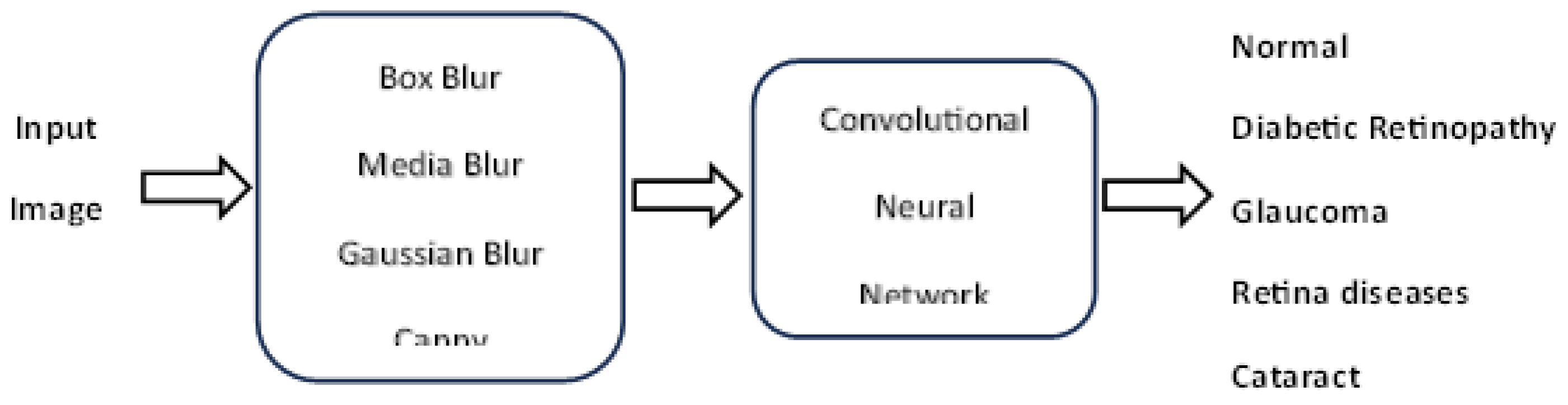
Figure 1 shows the flowchart illustrating the process for ocular disease classification.
The input image is pre-processed to obtain a clear, noise-free image, and an edge detector is applied to enhance the characteristics of each disease. These features are fed into a Convolutional Neural Network to classify eye diseases.
2.5 Dataset
Two datasets were used. From the first dataset, called Cataract Prediction [
16], the subset Retina_Disease was obtained; this subset does not include diabetic retinopathy. The second dataset was also obtained from Kaggle, and its name is Eye_Diseases_Classification [
17]; in this dataset are the subsets: Normal, Cataract, Diabetic Retinopathy, and Glaucoma diseases. Therefore, there are five classes, each with 200 instances, which means the dataset is balanced.
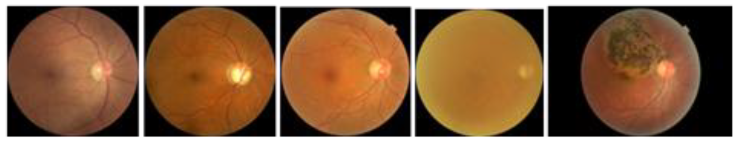
In
Figure 2, an example of the type of images that are handled in this work can be observed.
The two datasets were homogenized, and the dimensions of the resulting images were 250 x 250 pixels.
2.6 Pre-processing
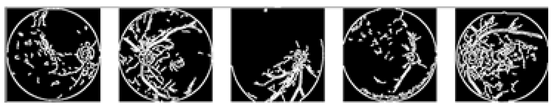
Images need to be cleaned to visualize their characteristics better and eliminate each impurity. This is achieved by applying various filters depending on what needs to be highlighted or eliminated. Therefore, the images were first changed to grayscale. The Blur filter was applied in a 3x3 matrix, followed by a Median Blur in a 5x5 matrix, and finally, a Gaussian filter in a 5x5 matrix to eliminate the largest number of impurities and soften the image. In this way, a sharper image could be obtained in terms of contrasts, thus obtaining clearer features and the desired result. Finally, the Canny filter is applied to get the edges and features representing each disease.
In
Figure 3, the results of the pre-processing step for the five classes are shown.
The images from
Figure 3 are fed to the Convolutional Neural Network to carry out the classification task.
2.7 Classification
The predictive model used is a custom Convolutional Neural Network (CNN) using TensorFlow and Keras. The network consists of 11 layers, including 3 Convolutional layers, 3 Max Pooling layers, 1 Batch Normalization layer, 1 Flattening layer, 2 Hidden layers, and 1 Output layer. Convolutional and Max Pooling layers allow to extract and reduce important features. Batch Normalization layers improve the performance and stability of deep neural networks by stabilizing activations and reducing overfitting, while Dense layers process these features to perform accurate classification. This architecture has been chosen for its effectiveness in image processing and pattern detection tasks.
3. Results
The complete code was programmed in Python, using OpenCV libraries for image pre-processing. TensorFlow and Keras libraries were used to build the CNN, an open-source library written in the same language. The characteristics of the computer with which the program was codified were the following:
8th generation Intel CORE i7 + processor at 2.2 GHz and Turbo Boost at 4GHz.
NVIDIA GEFORCE GTX 1050 graphics card
8 GB RAM
Windows 10 Home operating system
The validation method used was Hold-Out with 80% training and 20% testing.
The model was trained using the Adam optimization algorithm with a loss function primarily used for multiclass classification, and the accuracy metric was used to evaluate the performance of the model during training and validation. Early Stopping Callbacks were defined to prevent overfitting and restore the weights of the model that performed best on the validation set and Model Checkpoint to save the best-trained model. The model was trained using a data generator to increase the dataset size with a maximum of 100 epochs, and the validation set was used to monitor performance and prevent overfitting.
Below are the evaluation metrics that were applied to analyze the performance of our proposal.
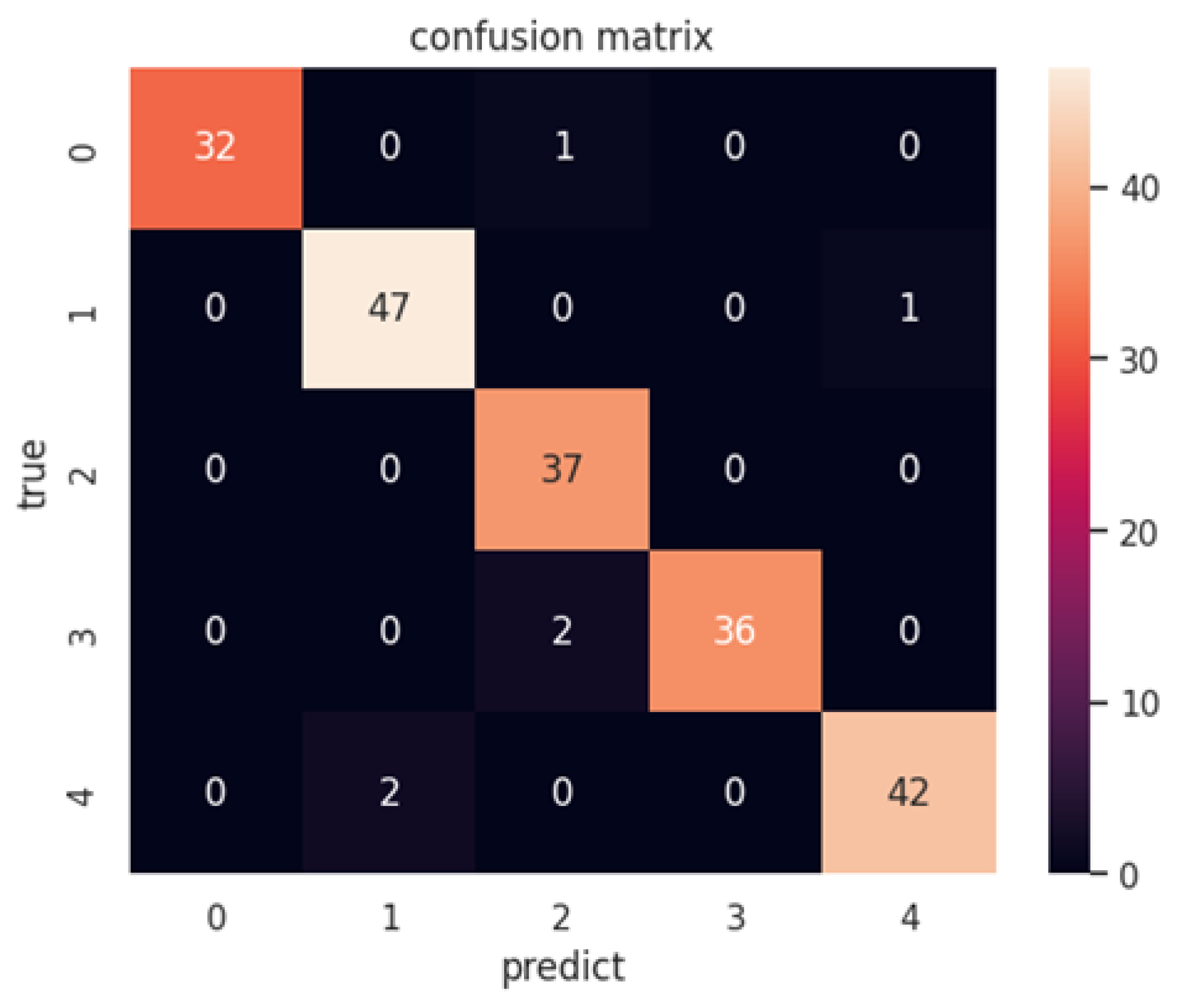
Figure 4 shows the results of the confusion matrix.
Confusion Matrix Analysis:
Class 0 (Glaucoma): It is observed that, of the 33 instances of glaucoma, 32 were correctly classified, with only one instance misclassified as another condition.
Class 1 (Cataract): For the 48 instances of cataract, 47 were correctly classified, and one was incorrectly classified.
Class 2 (Retina): Of the 37 instances of retinopathy, 36 were classified correctly, with one error.
Class 3 (Diabetic retinopathy): All 38 instances of diabetes were correctly classified, showing perfect performance in this class.
Class 4 (Normal): From the 44 normal instances, 43 were correctly classified, with only one error.
Table 2, shows the results of Precision.
The interpretation of
Table 2 is detailed as follows:
Macro: It is an arithmetic average of the accuracy of each class without considering class imbalance. A macro accuracy of 0.97218 indicates that, on average, the model has high accuracy for all classes.
Micro: Considers the total number of true positives and false positives at the global level. A micro precision of 0.97 shows that the overall performance of the model is very high.
Weighted: Weighted average of the precision of each class, considering the number of instances per class. This value is identical to micro, suggesting that the classes are balanced.
None: Individual precision for each class. The cataract, retina, and normal classes have lower accuracies (0.9591, 0.925, and 0.976, respectively), while the glaucoma and diabetes classes have perfect accuracy (1.0).
The accuracy results are presented in
Table 3.
Table 3.
Results of Accuracy: normalized and non-normalized.
Table 3.
Results of Accuracy: normalized and non-normalized.
| Accuracy |
| Normalized accuracy |
0.97 |
| Non-Normalized Accuracy |
194 |
The results in
Table 3 can be interpreted as follows:
Normalized Accuracy: Accuracy of 0.97 indicates that 97% of the predictions were correct.
Non-Normalized Accuracy: Indicates that 194 of the 200 instances in the test set were classified correctly.
Results from Recall metric are shown in
Table 4.
Recall, shown in
Table 4, measures the proportion of true positives over the total number of truly positive cases, as follows:
Macro: A value of 0.9701 shows that, on average, the model can identify all classes correctly.
Micro: A value of 0.97 indicates adequate overall performance of the model in correctly identifying positive cases.
Weighted: As with accuracy, the weighted value is 0.97, which suggests adequate overall performance.
None: Individual recall shows that the model has the most difficulty with glaucoma, cataract, diabetes, and normal classes (0.9696, 0.9791, 0.9473, 0.95454, respectively), while it has a perfect recall for retina (1.0).
Finally, the results for F
1-score are shown in
Table 5.
The F
1-score results in
Table 5 show that:
Macro: A macro F1-score of 0.9706 indicates that the overall performance of the model is high and balanced across all classes.
Micro: A micro F1-score of 0.97 confirms the good overall performance of the model.
Weighted: A weighted F1-score of 0.97 suggests that the model performs well.
None: The individual values reflect the same trends observed in accuracy and recall, with lower performance in retinopathy and glaucoma.
4. Discussion
Figure 4, which shows the confusion matrix, indicates that the algorithm used in this work performs correctly since it presents few erroneous data; the highest number of confusions is 2. In the case of precision (
Table 2), it can be observed that the classes of Glaucoma and Diabetic Retinopathy are correctly classified, while the other two diseases present an average precision of 0.94; however, the algorithm continues to show adequate performance when detecting if an image corresponds to a disease and differentiating it from a normal image. On the other hand, the Recall metric tells us that the average obtained from the four diseases is 0.974. At the same time, the normal class shows a Recall of 0.95, which, similarly to Precision, indicates that the algorithm can differentiate a normal image from a diseased one. Overall, the results show us two issues: our proposal can correctly distinguish a healthy eye from a diseased one, and it can adequately classify the four eye diseases.
From the results presented in the previous section, it can be observed that the average obtained from all the metrics used is 0.97. The number of classes to be analyzed was five: Glaucoma, Cataract, Retina diseases, Diabetic retinopathy, and Normal. In this context, the works related to our proposal will be compared;
Table 6 shows this comparison.
Table 6 shows that the works that handled four classes, Glaucoma, Cataract, Diabetic retinopathy, and Normal [
7,
8,
10], present an accuracy of between 94% and 99.1%. The algorithms that classified other data sets with more classes obtained an accuracy of between 60.31% and 99.1% [6,9,11-13]. Our proposal obtained an accuracy of 97% with five classes and linear filters, and a Convolutional Neural Network of our design was used, which decreases the complexity of the algorithm compared to the pre-trained models.
In future work, we intend to apply a different pre-processing to obtain images from which more main features can be extracted. We also have the idea of applying Siamese Convolutional Networks and analyzing their performance in relation to our proposal.
Table 6.
Comparison of our proposal against related works.
Table 6.
Comparison of our proposal against related works.
| Year |
Algorithm |
Classes |
Metrics |
| 2022 |
Vision Transformer-based approach with three architectures with 8, 14, 24 layers [6] |
Age-related macular degeneration, Cataracts, Diabetes, Glaucoma, Hypertension, and Myopia |
With 14 layers
F1-score=83.49%, sensitivity=84% precision= 83%, and Kappa score=0.802 |
| 2023 |
Single-Shot detection, Whale Optimization algorithm with Levy Flight and Wavelet search strategy, and ShuffleNet V2 model [7] |
Glaucoma, Cataract, Diabetic retinopathy and Normal |
Accuracy = 99.1%, Precision = 98.9%, Recall = 99%, F1 – Score = 98.9%, Kappa = 96.4%, Sensitivity = 98.9% and Specificity = 96.3%. |
| 2023 |
EfficientNetB0, VGG-16, and VGG-19 models [8] |
Glaucoma, Cataract, Diabetic Retinopathy and Normal |
With EfficientNetB0
Accuracy = 98.47%, Precision = 96.98%, Recall = 96.91%, and AUC = 99.84%. |
| 2023 |
CLAHE and Convolutional Neural Network [9] |
Glaucoma, cataract, diabetes, age-related macular degeneration, hypertension, and pathological myopia, as well as other diseases that are not specifically mentioned |
Experiment 1: multiclass classification
Accuracy=60.31% and AUC=85%
Experiment 2: Binary classification
Accuracy was between 98% and 100%, Recall from 97.99% to 100%, and Precision between 96% and 100%.
|
| 2023 |
Convolutional Neural Network and a pre-trained model: EfficientNet CNN [10] |
Glaucoma, Cataract, Diabetic retinopathy and Normal |
With EfficientNet CNN
Accuracy=94% |
| 2024 |
VGG-16 Convolutional Neural Network [11] |
Normal retina, Diabetic Macular Edema, Choroidal Neo-vascular Membranes, and Age-related Macular Degeneration |
Accuracy=94% and, after fine tuning, it approaches to 97%. |
| 2024 |
VGG-16, Xception and MobileNet for feature selection and CNN for classification [12] |
Choroidal neovascularization, Diabetic macular edema and Drusen and Normal |
MobileNet with CNN ensemble model
Accuracy of 95.34% |
| 2024 |
Fundus-DeepNet system [13] |
Normal, Diabetic retinopathy, Glaucoma, Cataracts, AMD, Myopia, Hypertension, and other abnormalities |
F1-score=88.56 %, Kappa score=88.92 %, and AUC= 99.76 % |
| 2024 |
Our proposal |
Glaucoma, Cataract, Retina diseases, Diabetic retinopathy and Normal |
Precision=97%, Accuracy=97%, Recall=97% and F1-score=97% |
Acknowledgments
The authors thank Instituto Politécnico Nacional (COFAA, SIP, and EDI) and SNII for their economic support in developing this paper.
References
- UNAM Global, En México, cerca de 1.5 millones de personas tienen glaucoma. Boletín: Número 221, CDMX, Ciudad Univer-sitaria.
- Piñero, R. , Lora, M., Andrés, M. I. Glaucoma, Offarm, 2005, Volume 24(2), pp. 88-96.
- Aliseda, D. and Berastegui, L. Retinopatía diabética. Anales Sis San Navarra [online]. 2008, Volume 31(3), pp.23-34.
- Tenorio, G., Ramírez-Sánchez, V. Retinopatía diabética: conceptos actuales. Revista Médica del Hospital General de México, 2010, Volume 73(3), pp. 193-201.
-
American Academy of Ophthalmology, https://www.aao.org/salud-ocular/enfermedades/que-son-las-cataratas.
- Dheeraj, S. and Ghosh, A. Classification of Ocular Diseases: A Vision Transformer-Based Approach. Innovations in Computa-tional Intelligence and Computer Vision, Lecture Notes in Networks and Systems 680, 2022. [CrossRef]
- Wahab, S. Artificial Intelligence-Driven Eye Disease Classification Model. Appl. Sci., 2023, Volume 13.
- Sener, B. and Sumer, E. Classification of Eye Disease from Retinal Images Using Deep Learning. 14th International Conference on Electrical and Electronics Engineering (ELECO), Bursa, Turkey, 30 Nov. – 2 Dec, 2023.
- Mostafa, K., Hany, M., Ashraf, A. and Mahmoud, M. Deep Learning-Based Classification of Ocular Diseases Using Convolu-tional Neural Networks, Intelligent Methods, Systems, and Applications (IMSA), Arab Republic of Egypt, July 15-16, 2023.
- Babaqi, T., Jaradat, M., Yildirim, A., Al-Nimer, S., and Won, D. Eye Disease Classification Using Deep Learning Techniques. Proceedings of the IISE Annual Conference & Expo, April 2023.
- Elkholy, M. and Marzouk, M.A. Deep learning-based classification of eye diseases using Convolutional Neural Network for OCT images. Front. Comput. Sci., 2024, Volume 5.
- Gulati, S., Guleria, K., Goyal, N. Detection and Multiclass Classification of Ocular Diseases using Deep Learning-based En-semble Model. International Journal of Intelligent Systems and Applications in Engineering, 2024, Volume 12(19s), pp. 18–29.
- Al-Fahdawi, S., Al-Waisy, A. S., Diyar Zeebaree, Q., Qahwaji, R., Natiq, H., Mohammed, M. A., Nedoma, J., Martinek, R., Deveci, M. Fundus-DeepNet: Multi-label deep learning classification system for enhanced detection of multiple ocular diseases through data fusion of fundus images. Information Fusion, 2024, Volume 102, pp. 1-11.
- Domínguez, T. Filtros de Procesamiento de Imágenes, In Visión artificial: Aplicaciones prácticas con Open CV – Python. 1st Ed., Marcombo, 2021, pp. 183-204.
- Moocarme, M., Abdolahnejad, M. and Bhagwat, R. Computer Vision with Convolutional Neural Netwoks. In The Deep Learning with Keras Workshop, 2nd Ed. Publisher: Packt Publishing Ltd. 2020.
- Cataract Prediction dataset. Available online: https://www.kaggle.com/datasets/jr2ngb/cataractdataset.
- Eye disease classification dataset. Available online: https://www.kaggle.com/datasets/gunavenkatdoddi/eye-diseases-classification.
|
Disclaimer/Publisher’s Note: The statements, opinions and data contained in all publications are solely those of the individual author(s) and contributor(s) and not of MDPI and/or the editor(s). MDPI and/or the editor(s) disclaim responsibility for any injury to people or property resulting from any ideas, methods, instructions or products referred to in the content. |
© 2025 by the authors. Licensee MDPI, Basel, Switzerland. This article is an open access article distributed under the terms and conditions of the Creative Commons Attribution (CC BY) license (https://creativecommons.org/licenses/by/4.0/).