Submitted:
10 February 2025
Posted:
12 February 2025
You are already at the latest version
Abstract
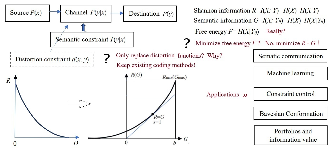
Does semantic communication require a semantic information theory parallel to Shannon's information theory, or can Shannon's work be generalized for semantic communication? This paper advocates for the latter and introduces the semantic information G theory (with "G" denoting generalization). The core approach involves replacing the distortion constraint with the semantic constraint, achieved by utilizing a set of truth functions as a semantic channel. These truth functions enable the expression of semantic distortion, semantic information measures, and semantic information loss. Notably, the maximum semantic information criterion is shown to be equivalent to the maximum likelihood criterion and parallels the Regularized Least Squares criterion. The G theory is compatible with machine learning methodologies, offering enhanced capabilities for handling latent variables, often addressed through Variational Bayes. This paper systematically presents the generalization of Shannon's information theory into the G theory and its wide-ranging applications. The applications involve semantic communication, machine learning, constraint control, Bayesian confirmation, portfolio theory, and information value. Furthermore, insights from statistical physics are discussed: Shannon information is equated to free energy, semantic information to the free energy of local equilibrium systems, and information efficiency to the efficiency of free energy in performing work. The paper also proposes refining Friston's minimum free energy principle into the maximum information efficiency principle. Lastly, it discusses the limitations of the G theory in representing the semantics of complex data.
Keywords:
semantic information theory
; semantic information measure
; information rate-distortion
; information rate-fidelity
; variational Bayes
; minimum free energy
; maximum information efficiency
; portfolio
; information value
; constraint control
1. Introduction
Although Shannon's information theory [1] has achieved remarkable success, it faces three
significant limitations that restrict its semantic communication and machine
learning applications. First, it cannot measure semantic information. Second,
it relies on the distortion function to evaluate communication quality, but the
distortion function is subjectively defined and lacks an objective standard.
Third, it is challenging to incorporate model parameters into entropy formulas.
In contrast, machine learning often requires cross-entropy and cross Mutual
Information (MI) involving model parameters (Appendix
A lists all abbreviations with original texts). Moreover, the minimum
distortion criterion resembles the philosophy of "absence of fault is a
virtue," whereas a more desirable principle might be "merit
outweighing fault is a virtue." Why did Shannon's information theory use
the distortion criterion instead of the information criterion? This is
intriguing.
The study of semantic information gained attention
soon after Shannon's theory emerged. Weaver initiated research on semantic
information and information utility [2], and
Carnap and Bar-Hillel proposed a semantic information theory [3]. Thirty years ago, the author of this article
extended Shannon's theory to a semantic information framework [4,5,6,7], now known as the semantic information G
theory (abbreviated as the G theory) [8].
Here, "G" stands for generalization, reflecting the G theory's role
as a generalized form of Shannon's information theory. Earlier contributions to
semantic information theories include works by Carnap and Bar-Hillel, Dretske [9], Wu [10], and
Zhong [11], while more recent contributions
after the author's generalization include those by Floridi [12,13] and others [14].
These theories primarily address natural language information and semantic
information measures (upstream problems). In contrast, newer approaches have
focused on electronic semantic communication over the past decade, particularly
semantic compression (downstream problems) [14,15,16,17].
These explorations are highly valuable.
Researchers hold two extreme views on semantic
information theory. One view argues that Shannon's theory suffices, rendering a
dedicated semantic information theory unnecessary; at most, semantic distortion
needs consideration; the opposing view advocates for a parallel semantic
information theory alongside Shannon's framework. Among parallel approaches,
some researchers (e.g., Carnap and Bar-Hillel) use only logical probability,
avoiding statistical probability, while others incorporate semantic sources, semantic
channels, semantic destinations, and semantic information rate distortion [17].
The G theory offers a compromise between these
extremes. It fully inherits Shannon's information theory, including its derived
theories. Only the semantic channel composed of truth functions is newly added.
Based on Davidson's truth-conditional semantics [18],
truth functions represent the extensions and semantics of concepts or labels.
By leveraging the semantic channel, the G theory can:
- derive the likelihood function from the truth function and source, enabling semantic probability predictions, thereby quantifying semantic information, and
- replace the distortion constraint in Shannon's theory with semantic constraints, which include semantic distortion, semantic information quantity, and semantic information loss constraints.
The semantic information measure does not replace
Shannon's information measure but supplants the distortion metric used to
evaluate communication quality. Truth functions can be derived from sample
distributions using machine learning techniques with the maximum semantic
information criterion, addressing the challenges of defining classic distortion
functions and optimizing Shannon channels with an information criterion. A key
advantage of generalization over reconstruction is that semantic constraint functions
can be treated as new or negative distortion functions, allowing the use of
existing coding methods without additional electronic semantic communication
coding considerations.
In addition to Shannon's ideas, the G theory
integrates Popper's views on semantic information, logical probability, and
factual testing [19,20]; Fisher's maximum
likelihood principle [21]; and Zadeh's fuzzy
set theory [22,23]. To unify Popper's logical
probability with Zadeh's fuzzy sets, the author proposed the P-T probability
framework [8,24], simultaneously accommodating
both statistical and logical probabilities.
Thirty years ago, the G theory was applied to image
data compression based on visual discrimination [5,7].
In the past decade, the author has introduced model parameters into truth
functions, utilized truth functions as learning functions [7,25], and optimized them with sample
distributions. The G theory has also been employed to optimize semantic
communication for machine learning tasks, including multi-label learning,
maximum MI classification, mixture models [8],
Bayesian confirmation [26,27], semantic
compression [28], constraint control [29], and latent variable solutions [30]. The concept of mutually aligning semantic and
Shannon channels aids in understanding decentralized machine learning and
reinforcement learning methods.
The main motivations and objectives of this paper
are as follows:
Semantic communication urgently requires a semantic
compression theory analogous to the information rate-distortion theory [31,32,33]. The author extends the information
rate-distortion function to derive the information rate fidelity function R(G)(where
R is the minimum Shannon MI for a given semantic MI G), which
provides a theoretic foundation for semantic compression theory.
Estimated MI (a specific case of semantic MI) [25,34,35] and Shannon MI minimization [36] have been utilized in deep learning. However,
researchers often conflate estimated MI with Shannon MI and remain unclear
about which should be maximized or minimized [37,38,39].
The G theory can clarify these distinctions.
The G theory has undergone continuous refinement,
with many results scattered across more than 20 articles by the author. This
paper aims to provide a comprehensive overview, helping future researchers
avoid redundant efforts.
The remainder of this paper is organized as
follows: Section 2 introduces the G
theory; Section 3 discusses electronic
semantic communication; Section 4
explores goal-oriented information and information value (in conjunction with
portfolio theory); and Section 5 examines
the G theory's applications to machine learning. The final section provides
discussions and conclusions, including comparing the G theory with other
semantic information theories, exploring the concept of information, and
identifying the G theory's limitations and areas for further research.
2. From Shannon's Information Theory to the Semantic Information G Theory
2.1. Semantics and Semantic Probabilistic Predictions
Popper stated in his 1932 book The Logic of
Scientific Discovery [19] (p. 102): the
significance of scientific hypotheses lies in their predictive power, and
predictions provide information; the smaller the logical probability and the
more it can withstand testing, the greater the amount of information it
provides. He also explicitly emphasized the necessity of distinguishing between
two types of probability: statistical probability and logical probability. The
G theory incorporates two kinds of probabilities and probability predictions,
with T representing logical probability and truth value. Statistical
probability predictions are expressed using Bayes' formula, and semantic
probability predictions follow a similar approach.
The semantics of a word or label encompass both its
connotation and extension. Connotation refers to an object's essential
attributes, while extension denotes the range of objects the term refers to.
For example, the extension of "adult" includes individuals aged 18
and above, while its connotation is "over 18 years old." Extensions
for some concepts, like "adult," may be explicitly defined by
regulations, whereas others, such as "elderly," "heavy
rain," "excellent grades," or "hot weather," are more
subjective and evolve through usage. Connotation and extension are
interdependent; one can often infer one from the other.
According to Tarski's truth theory [40] and Davidson's truth-conditional semantics [9], a concept's semantics can be represented by a
truth function, which reflects the concept's extension. For a crispy set, the
truth function acts as the characteristic function of the set. For example, x
is age, and y1 is the label of the set {adult}, we denote
the truth function as T(y1|x), which is also the
characteristic function of the set {adult}.
In 1931, Popper put forward in the book "The
Logic of Scientific Discovery" [39]
(P.96) that the smaller the logical probability of a scientific hypothesis, the
greater the amount of (semantic) information if it can stand the test. We can
say that Popper is the earliest researcher of semantic information [19]. Later, he proposed a logical probability axiom
system. He emphasized that there are two kinds of probabilities, statistical
and logical probabilities, at the same time ([39]
(pp. 252-258). But he had not established a probability system that includes
both.
The truth function serves as the tool for semantic
probability predictions (illustrated in Figure 1).
The formula is:
If "adult" is changed to
"elderly", the crispy set becomes a fuzzy set, the truth function is
equal to the membership function of the fuzzy set, and the above formula
remains unchanged.
The extension of a sentence can be regarded as a
fuzzy range in a high-dimensional space. For example, an instance described by a
sentence with a subject, object, and predicate structure can be regarded as a point
in the Cartesian product of three sets, and
the extension of a sentence is a fuzzy subset in the Cartesian
product. For example, the subject and the predicate are two people in
the same group, and the predicate can be selected as one of "bully",
"help", etc. The extension of "Tom helps Jone" is an
element in the three-dimensional space, and the extension of "Tom helps an
old man" is a fuzzy subset in the three-dimensional space. The extension
of a weather forecast is a subset in the multidimensional space with time,
space, rainfall, temperature, wind speed, etc., as coordinates. The extension
of a photo or a compressed photo can be regarded as a fuzzy set, including all
things with similar characteristics.
Floridi affirms that all sentences or labels that may
be true or false contain semantics and provide semantic information [26]. The author agrees with this view and suggests
converting the distortion function and the truth function T(yj|x)
to each other. To this end, we define:
T(yj|x) ≡ exp[–d(yj|x)],
d(yj|x) ≡ –logT(yj|x).
where exp and log are a pair of inverse functions; d(yj|x)
means the distortion when yj represents xi.
We use d(yj|x) instead of d(x, yj)
because the distortion may be asymmetrical.
For example, the pointer on a Global Positioning
System (GPS) map has relative error or distortion; the distortion function can
be converted to a truth function or similarity function:
T(yj|x)=exp[–d(yj|x)]=exp[–(x–xj)2/(2σ2)],
where σ is the standard deviation; the
smaller it is, the higher the precision. Figure 2 shows the mobile phone positioning seen by someone on a train.
According to the semantics of the GPS pointer, we
can predict that the actual position is an approximate normal distribution on
the high-speed rail, and the red five-star indicates the maximum possible
position. If a person is on a specific highway, the prior probability
distribution P(x) will change, and the maximum possible position
is the place closest to the small circle on that highway.
Clocks, scales, thermometers, and various economic
indices are similar to the positioning pointers and can all be regarded as
estimates (), with error ranges or extensions, so they can all
be used for semantic probability prediction and provide semantic information.
Color perception can also be regarded as an estimate of color or color light.
The higher the discrimination of the human eye (similar to the smaller σ),
the smaller the extension. A Gaussian function can also express its truth
function or discrimination function.
2.2. The P-T Probability Framework
Carnap and Bar-Hillel only use logical probability.
We use logical probability, truth value, and statistical probability in the
above semantic probability prediction. The truth value is conditional logical
probability. The G theory is based on the P-T probability framework.
Why do we need a new probabilistic framework?
Because a hypothesis or label, such as "adult", has two probabilities
simultaneously. One is the probability of the set represented by the label,
which is defined by Kolmogorov [41]; it is not
normalized. Another is the probability in which the label is selected. It is
defined by Mises [42]; it is normalized. The
P-T probability framework attempts to unify the two probabilities and
generalize the set to the fuzzy set.
We define:
- X and Y are two random variables, taking x ϵ U={x1, x2, …} and y ϵ V ={y1, y2, …} as their values. For machine learning, xi is an instance, and yj is a label or hypothesis; yj(xi) is a proposition, and yj(x) is a proposition function.
- The θj is a fuzzy subset of the domain U, whose elements make yj true. We have yj(x) = "x ϵ θj". The θj can also be understood as a model or a set of model parameters.
- Probability defined by “=”, such as P(yj)≡P(Y = yj), is a statistical probability; probability defined by “ϵ”, such as P(X ϵ θj), is a logical probability. To distinguish P(Y = yj) and P(X ϵ θj), we define the logical probability of yj as T(yj)≡ T(θj)≡ P(X ϵ θj).
- T(yj|x) ≡ T(θj|x)≡ P(X ϵ θj|X = x)∈[0,1] is the truth function of yj and also the membership function mθj(x) of the fuzzy set θj, that is,
T(yj|x) ≡ T(θj|x)≡mθj
(x).
The logical probability of a label is generally not
equal to its statistical probability. The logical probability of a tautology is
1, while its statistical probability is close to 0. We have P(y1)
+ P(y2) + … + P(yn) = 1, but
it is possible that T(y1) + T(y2)
+ … + T(yn) > 1. For example, the age labels
include "adult", "non-adult", "child",
"youth", "elderly", etc., and the sum of their statistical
probabilities is 1, while the sum of their logical probabilities is greater
than 1 because the sum of the logical probabilities of "adult" and
"non-adult" alone is equal to 1.
According to the above definition, we have:
This is the probability of a fuzzy event defined by
Zadeh [23].
We can put T(θj|x) and P(x)
into the Bayesian formula to obtain the semantic probability prediction
formula:
To
P(x|θj) is the likelihood function P(x|yj,
θ) in the popular method. We use P(x|θj) here
because the j-th parameter is bound to yj. We call the
above formula the semantic Bayesian formula:
Because the maximum value of T(yj|x)
is 1, from P(x) and P(x|θj), we
derive a new formula:
2.3. Semantic Channel and Semantic Communication Model
Shannon calls P(X), P(Y|X),
and P(Y) the source, the channel, and the destination. Just as a
set of transition probability functions P(yj|x)( j=1,
2, …) constitutes a Shannon channel, a set of truth value functions T(θj|x)
(j=1,2,…) constitutes a semantic channel. The comparison of the two
channels is shown in Figure 3. For
convenience, we also call P(x), P(y|x), and P(y)
the source, the channel, and the destination, and we call T(y|x)
the semantic channel.
The semantic channel reflects the semantics or
extensions of labels, while the Shannon channel indicates the usage of labels.
The comparison between the Shannon and the semantic communication models is
shown in Figure 4. The distortion
constraint is usually not drawn, but it actually exists.
The semantic channel contains information about the
distortion function, and the semantic information represents the communication
quality, so there is no need to define a distortion function anymore.
Optimizing the model parameters is to make the semantic channel match the
Shannon channel, that is, T(θj|x)∝P(yj|x)
or P(x|θj) = P(x|yj) (j=1,2,…),
so that the semantic MI reaches its maximum value and is equal to the Shannon
information. Conversely, when the Shannon channel matches the semantic channel,
the information difference reaches the minimum, or the information efficiency
reaches the maximum.
2.4. Generalizing Shannon Information Measure to Semantic Information G Measure
Shannon MI can be expressed as.
where H(X) is the entropy of X,
reflecting the minimum average code length. H(X|Y) is the
posterior entropy of X, reflecting the minimum average code length after
predicting x based on Y. Therefore, Shannon MI means the average
code length saved due to the prediction.
We replace P(xi|yj)
on the right side of the log with the likelihood function P(xi|θj).
Then we get the semantic MI:
where H(X|Yθ) is
the semantic posterior entropy of x:
H(X|Yθ) is the free energy
F in the Variational Bayes method (VB) [44,45]
and the Minimum Free Energy (MFE) principle [46].
The smaller it is, the greater the amount of semantic information. H(Yθ|X)
is called the fuzzy entropy, equal to the average distortion . Because according to Equation (2), there is:
H(Yθ) is the semantic
entropy:
Note that P(x|yj) on the
left side of the log is used for averaging and represents the sample
distribution. It can be a relative frequency and may not be smooth or
continuous. P(x|θj) and P(x|yj)
may differ, reflecting that obtaining information needs factual testing. It is
easy to see that the maximum semantic MI criterion is equivalent to the maximum
likelihood criterion and is similar to the Regularized Least Squares (RLS)
criterion. Semantic entropy is the regularization term. Fuzzy entropy is a more
general average distortion than the average square error.
Semantic entropy has a clear coding meaning. Assume
that the sets θ1, θ2, … are crispy sets;
the distortion function is:
We regard P(Y) as the source and P(X)
as the destination, then the parameter solution of the information
rate-distortion function is [31]:
It can be seen that the minimum Shannon MI is equal
to the semantic entropy, that is, R(D=0)=H(Yθ).
The following formula indicates the relationship
between Shannon MI and semantic MI and the encoding significance of semantic
MI:
where KL(…) is the Kullbak-Leibler (KL) divergence
with a likelihood function, which Akaike [43] first
used to prove that the minimum KL divergence criterion is equivalent to the
maximum likelihood criterion. The last term in the above formula is always
greater than 0, reflecting the average code length of residual coding.
Therefore, the semantic MI is less than or equal to the Shannon MI; it reflects
the average code length saved due to semantic prediction.
From the above formula, the semantic MI reaches its
maximum value when the semantic channel matches the Shannon channel. According
to Equation (15), letting P(x|θj)= P(x|yj),
we can obtain the optimized truth function from the sample distribution:
When Y=yj, the semantic MI becomes the semantic KL information:
The KL divergence cannot usually be interpreted as information because the smaller it is, the better. But I(X; θj) above can be said to be information because the larger it is, the better.
Solving T*(θj|x) with equation (16) requires that the sample distributions P(x) and P(x|yj) are continuous and smooth. Otherwise, by using Equation (17), we can obtain:
The above method for solving T*(θj|x) is called Logical Bayesian Inference (LBI) [8] and can be called the random point falling shadow method. This method inherits Wang's idea of random set falling shadow [47,48].
Suppose the truth function in (10) becomes a similarity function. In that case, the semantic MI becomes the estimated MI [25], which has been used by deep learning researchers for Mutual Information Neural Estimation (MINE) [34] and Information Noise Contrast Estimation (InfoNCE) [35].
In the semantic KL information formula, when X=xi, I(X; θj) becomes the semantic information between a single instance xi and a single label yj:
The above formula reflects Popper's idea about factual testing. Figure 5 illustrates the above formula. It shows that the smaller the logical probability, the greater the absolute value of the information; the greater the deviation, the smaller the information; wrong assumptions convey negative information.
Bring Equation (2) into (19), we have
I(xi; θj)=log[1/T(θj)] – d(yj|x),
which means I(X; θj) equals Carnap and Bar-Hillel's semantic information minus distortion. If T(θj|x) is always 1, the two amounts of information become equal.
2.5. From the Information Rate-distortion Function to the Information Rate-fidelity Function
Shannon defines that given a source P(x), a distortion function d(y|x), and the upper limit D of the average distortion , we change the channel P(y|x) to find the minimum MI R(D). R(D) is the information rate-distortion function, which can guide us in using Shannon information economically.
Now, we replace d(yj|xi) with I(xi; θj), replace with I(X; Yθ), and replace D with the lower limit G of the semantic MI to find the minimum Shannon MI R(G). R(G) is the information rate-fidelity function. Because G reflects the average code length saved due to semantic prediction, Using G as the constraint is more consistent in shortening the code length, and G/R can better reflect information efficiency.
The author uses the word "fidelity" because Shannon originally proposed the information rate-fidelity criterion [12], and later used minimum distortion to express maximum fidelity. The author has previously referred to R(G) as "the information rate of keeping precision" [16] or "information rate-verisimilitude" [25].
The R(G) function is defined as
We use the Lagrange multiplier method to find the minimum MI. The Lagrangian function is:
Using P(y|x) a variation, we let . Then, we obtain:
where mij=P(xi|θj)/P(xi)=T(θj|xi)/T(θj). Using P(y) a variation, we let . Then, we obtain:
where P+1(yj) means the next P(yj). Because P(y|x) and P(y) are interdependent, we can first assume a P(y) and then repeat the above two formulas to obtain convergent P(y) and P(y|x) (see [33] (P. 326)). We call this method the Minimum Information Difference (MID) iteration.
Any R(G) function is bowl-shaped (possibly not symmetrical) [6], with the second derivative greater than 0. The s = dR/dG is positive on the right. When s = 1, G equals R, meaning the semantic channel matches the Shannon channel. G/R represents information efficiency; its maximum is 1. G has a maximum value G+ and a minimum value G– for given R. G– means how small the semantic information the receiver receives can be when the sender intentionally lies.
We can apply the R(G) function to image compression based on visual discrimination [5,6], maximum MI classification of unseen instances, the convergence proof of mixture models [7], and semantic compression [28].
It is worth noting that, given a semantic channel T(y|x), matching the Shannon channel with the semantic channel, i.e., letting P(yj|x) ∝ T(yj|x) or P(x|yj) = P(x|θj), does not maximize the semantic MI, but minimizes the information difference between R and G or the information efficiency G/R. Then, we can increase G and R simultaneously by increasing s. When s-->∞ in Equation (23), P(yj|x) (j = 1, 2, …, n) only takes the value 0 or 1, becoming a classification function.
We can also replace the average distortion with fuzzy entropy H(Yθ|X) (using semantic distortion constraints) to obtain the information rate truth function R(Θ) [28]. In situations where information rather than truth is more important, R(G) is more appropriate than R(D) and R(Θ). P(y) and P(y|x) obtained for R(Θ) are different from those obtained for R(G) because the optimization criteria are different. Under the minimum semantic distortion criterion, P(y|x) becomes:
where T(θxi|y) is a constraint function so that the distortion function d(xi|y) =–log T(θxi|y). R(Θ) becomes R(D). If T(θj) is small, the P(yj) required for R(G) will be larger than the P(yj) required for R(D) or R(Θ).
2.6. Semantic Channel Capacity
Shannon calls the maximum MI obtained by changing the source P(x) for the given Shannon channel P(y|x) the channel capacity. Because the semantic channel is also inseparable from the Shannon channel, we must provide both the semantic and Shannon channels to calculate the semantic MI. Therefore, after the semantic channel is given, there are two cases: 1) the Shannon channel is fixed; 2) we must first optimize the Shannon channel according to a specific criterion.
When the Shannon channel is fixed, the semantic MI is less than the Shannon MI, so the semantic channel capacity is less than or equal to the Shannon channel capacity. The difference between the two is shown in Equation (15).
If the Shannon channel is variable, we can use the MID iteration to find the Shannon channel for R=G after each change of the source P(x), and then use s––>∞ to find the Shannon channel P(y|x) that makes R and G reach their maxima simultaneously. At this time, P(y|x)∈{0,1} becomes the classification function. Then, we calculate the semantic MI. For different P(x), the maximum semantic MI is the semantic channel capacity. That is
where Gmax is G+ when s—>∞ (see Figure 6). Hereafter, the semantic channel capacity only refers to CT(y|x) in the above formula.
Practically, to find CT(Y|X), we can look for x(1), x(2), …, x(j) ∈ U, which are instances under the highest points of T(y1|x), T(y2|x), …, T(yn|x) respectively. Let P(x(j))=1/n, j=1, 2, …, n, and the probability of any other x equals 0. Then we can choose the Shannon channel: P(yj|x(j))=1, j=1, 2, …, n. At this time, I(X; Y))=H(Y)=logn, which is the upper limit of CT(Y|X). If there is xi among the n x(j)s, which makes more than one truth function true, then either T(yj)>P(yj) or the fuzzy entropy is not 0. CT(Y|X) will be slightly less than logn in this case.
According to the above analysis, the encoding method to increase the capacity of the semantic channel is:
- .Try to choose x that only makes one label's true value 1 (avoid ambiguity and reduce the logical probability of y);
- Encoding should make P(yj|xj)=1 as much as possible (to ensure that Y is used correctly).
- Choose P(x) so that each Y's probability and logical probability are as equal as possible (close to 1/n, thereby maximizing the semantic entropy).
3. Electronic Semantic Communication Optimization
3.1. Electronic Semantic Communication Model
The previous discussion of semantic communication did not consider conveying semantic information by electronic communication. Assuming that the time and space distance between the sender and the receiver is very far, we must transmit information through cables or disks. At this time, we need to add an electronic channel based on the previous communication model, as shown in Figure 7:
Electronic semantic communication is still electronic communication, in essence. The difference is that we need to use semantic information loss instead of distortion as the optimization criterion. The choice of Y includes the optimization of the semantic channel P(y|x) and the Shannon channel T(y|x) between x and y.
3.2. Optimization of Electronic Semantic Communication with Semantic Information Loss as Distortion
Consider electronic semantic communication. If there is no distortion, that is, ŷj=yj, the semantic information about x transmitted by both is the same, and there is no semantic information loss. If ŷj ≠ yj, there is semantic information loss. Farsad et al. call it the semantic error and propose the corresponding formula [49,50]. Papineni et al. also proposed a similar formula for translation [51]. For more discussion, see [52].
According to the G theory, the semantic information loss caused by using ŷj instead of yj is:
LX(yj||ŷj) is a generalized KL divergence because there are three functions. It indicates the average code length of residual coding.
Since the loss is generally asymmetric, there may be LX(yj||ŷj)≠LX(yj||ŷj). For example, when "motor vehicle" and "car" are substituted for each other, the information loss is asymmetric. The reason is that there is a logical implication relationship between the two. Using "motor vehicle" to replace "car", although it reduces information, it is not wrong; while using "car" to replace "motor vehicle" may be wrong, because the actual may be a truck or a motorcycle. When an error occurs, the semantic information loss is enormous. An advantage of using the truth function to generate the distortion function is that it reflects concepts' implications or similarity relationships.
Assuming that yj is the correct label used, it comes from sample learning, so P(x|θj)=P(x|yj), and LX(yj||ŷj)=KL(P(x|θj)||P(x|j)). The average semantic information loss is:
Consider using P(y) as the source and P(Ŷ) as the destination to encode y. Let d(ŷk|yj)=LX(yj||ŷk); we can obtain the information rate-distortion function R(D) for replacing Y with Ŷ. We can code Y for data compression according to the parameter solution of the R(D) function.
In the electronic communication part (from Y to Ŷ), other problems can be resolved by classical electronic communication methods, except for using semantic information loss as distortion.
If finding I(x;j) is not too difficult, we can also use I(x;j) as a negative distortion function. Minimizing I(X; ŷ) for given when G= I(X; ŷθ), we can get the R(G) function between x and Ŷ and compress the data accordingly.
3.3. Experimental Results: Compress Image Data According to Visual Discrimination
The simplest visual discrimination is the discrimination of human eyes to different colors or gray levels. The nest is the spatial discrimination of points. Suppose the movement of a point on the screen is not detected. In that case, the fuzzy movement range can represent the spatial position discrimination, which can be represented by a truth function (such as the Gaussian function). What is more complicated is to distinguish whether two figures are the same person. Advanced image compression needs to extract image features like Autoencoder and use features to represent images. The following methods need to be combined with the feature extraction method in deep learning to get better applications.
The simplest gray-level discrimination is taken as an example to illustrate digital image compression.
1) Measuring Color Information
A color can be represented by a vector (B, G, R). For convenience, we assume that the color is one-dimensional (or we only consider the gray level), expressed in x, and the color sense Y is the estimation of x, similar to the GPS indicator. The universes of x and Y are the same, and yj="x is about xj". If the color space is uniform, the distortion function can be defined by distance, that is, d(yj|x) = exp[–(x–xj)2/(2σ2)]. Then there is the average information of color perception, I(X; Yθ)=H(Yθ)–.
Given the source P(x) and the discrimination function T(y|x), we can solve P(y|x) and P(y) using the SVB method. The Shannon channel is matched with the semantic channel to maximize the information efficiency.
2) Gray Level Compression
We use an example to illustrate color data compression. Assuming that the original gray level is 256 (8-bit pixels) and is now compressed into 8 (3-bit pixels), we can define eight constraint functions, as shown in Figure 8a.
Considering that human visual discrimination varies with the gray level (the higher the gray level, the lower the discrimination), we use the eight truth functions shown in Figure 8a, representing eight fuzzy ranges. Appendix C in Reference [28] shows how these curves are generated. The task is to use the Maximum Information Efficiency (MIE) criterion to find the Shannon channel P(y|x) that makes R close to G (s=1).
The convergent P(y|x) is shown in Figure 8b. Figure 8c shows that Shannon MI and semantic MI gradually approach in the iteration process. Comparing figures 8a and 8b, we find it easy to control P(y|x) by T(y|x). However, defining the distortion function without using the truth function is difficult. It is also difficult to predict the convergent P(y|x) by d(y|x).
If we use s to strengthen the constraint, we get the parametric solution of the R(G) function. As s→∞, P(yj|x) (j=1,2,…) display as rectangles and becomes classification functions.
3) Influence of Discrimination and Quantization Level on the R(G) Function
Consider the semantic information of gray pixels. The discrimination function determines the semantic channel T(y|x), and the source entropy H(X) increases with the quantization level b=2n (n is the number of quantization bits). Figure 9 shows that when the quantization level is enough, the R and G variation range increases with the discrimination increasing (i.e., with σ decreasing). The discrimination determines the semantic channel capacity.
4. Goal-Oriented Information, Information Value, Physical Entropy and Free Energy
4.1. Three Kinds of Information Related to Value
We call the increment of utility the value. Information involves utility and value in three aspects:
1)Information about utility. For example, the information about university admission or the bumper harvest of grain is about utility.
The measurement of this information is the same as the previous semantic information measurement. Before providing information, we have the prior probability distribution P(x) of grain production. The information is provided in the form of range, such as "about 2000 kg per acre", which can be expressed by a truth function. The previous semantic information formula is also applicable.
2) Goal-oriented information. It is also purposeful information or constraint control feedback information.
For example, a passenger and a driver watch GPS maps in a taxi. Assume that the probability distribution of the taxi position without looking at the positioning map (or without some control) is P(x), and the destination is a fuzzy range, which a truth function can represent. The actual position is the probability distribution P(x|aj) (conditioned on action aj). The positioning map provides information. For the passenger, this is purposeful information (about how the control result comforts the purpose); for the driver, this is the control feedback information. We call both goal-oriented information. This information involves constraint control and reinforcement learning. The following section discusses the measurement and optimization of this information.
3) Information that brings value. For example, Tom made money by buying stocks based on John's prediction of stock prices. The information provided by John brings Tom increased utility, so John's information is valuable to Tom.
The value of information is relative. For example, weather forecast information is different for workers and farmers, and forecast information about stock markets is worth 0 to people who do not buy stocks. The value of information is often difficult to judge. For example, defining value losses due to missed reporting and false reporting is difficult regarding medical cancer tests. In most cases, missed reporting of low-probability events often causes more loss than false reporting, such as for medical tests and earthquake forecasts. In these cases, the semantic information criterion can be used to reduce missed reporting of low-probability events.
For investment portfolios, quantitative analysis of information value is possible. Section 4.3 focuses on the information value of portfolios.
4.2. Goal-Oriented Information
4.2.1. Similarities and Differences Between Goal-Oriented Information and Prediction Information
Previously, we used the G measure to measure prediction information, requiring the prediction P(x|θj) to conform to the fact P(x|yj). Goal-oriented information is the opposite, requiring the fact to conform to the purpose.
An imperative sentence can be regarded as a control instruction. We need to know whether the control result conforms to the control purpose. The more consistent the result is, the more information there is.
A truth function or a membership function can represent a control target. For example, there are the following targets:
- "Workers' wages should preferably exceed 5000 dollars";
- "The age of death of the population had better exceed 80 years old";
- "The cruising distances of electric vehicles should preferably exceed 500 kilometers";
- "The error of train arrival time had better be less than one minute".
The semantic KL information formula can measure purposeful information:
In the formula, θj is a fuzzy set, indicating that the control target is a fuzzy range. yj here becomes aj, indicating the action corresponding to the j-th control task yj. If the control result is a specific xi, the above formula becomes the semantic information I(xi; aj|θj).
If there are several control targets y1, y2,… we can use the semantic MI formula to express the purposeful information:
where A is a random variable taking a value a or aj. Using SVB, the control ratio P(a) can be optimized to minimize the control complexity (i.e., Shannon MI) when the purposive information is the same.
4.2.2. Optimization of Goal-Oriented Information
Goal-oriented information can be regarded as the cumulative reward in constraint control. However, the goal here is a fuzzy range, which is expressed by a plan, command, or imperative sentence. The optimization task is similar to the active inference task using the MFE principle [46].
The semantic information formulas of imperative and descriptive (or predictive) sentences are the same, but the optimization methods differ (see Figure 10). For descriptive sentences, the fact is unchanged, and we hope that the predicted range conforms to the fact, that is, fix P(yj|x) so that T(θj|x)∝P(yj|x), or fix P(x|yj) so that P(x|θj)=P(x|yj). For imperative sentences, we hope that the fact conforms to the purpose, that is, fix T(θj|x) or P(x|θj), and minimize the information difference or maximize the information efficiency G/R by changing P(yj|x) or P(x|yj), or balance between the purposiveness and the efficiency.
For multi-target tasks, the objective function to be minimized is:
f = I(X; A) – sI(X;A/θ).
When the actual distribution P(x|aj) is close to the constrained distribution P(x|θj), the information efficiency (not information) reaches its maximum value of 1. To further increase the two types of information, we can use the MID iteration formula to obtain:
Because the optimized P(x|aj) is a function of θj and s, we write P*(x|aj)=P(x|θj, s). It is worth noting that many distributions P(x|aj) satisfy the constraint and maximize I(X; aj/θj), but only P*(x|aj) minimizes I(X; aj).
4.2.3. Experimental Results: Trade-Off Between Maximizing Purposiveness and MIE
Figure 11shows a two-objective control task, with objectives represented by the truth functions T(θ0|x) and T(θ1|x). We can imagine these as two pastures with fuzzy boundaries where we need to herd sheep. Without control, the density distribution of the sheep is P(x). We need to solve an appropriate distribution P(a).
For different s, we set the initial proportions: P(a0)=P(a1)=0.5. Then, we used (33) and (34) for the MID iteration to obtain proper P(aj|x) (j=0,1). Then, we got P(x|aj)=P(x|θj,s) by using (33). Finally, we obtained G(s), R(s), and R(G) by using (25).
The dashed line for R1(G) in Figure 12 indicates that if we replace P(x|aj)=P(x|θj, s) with a normal distribution, P(x|βj, s), G and G/R1 do not obviously become worse.
4.3. Investment Portfolios and Information Values
4.3.1. Capital Growth Entropy
Markowitz's portfolio theory [53] uses a linear combination of expected income and standard deviation as the optimization criterion. In contrast, the compound interest theory of portfolios uses compound interest, i.e., geometric mean income, as the optimization criterion.
The compound interest theory began with Kelley [54], followed by Latanne and Tuttle [55], Arrow [56], Cover [57], and the author of this article. The famous American information theory textbook "Elements of Information Theory" [58] co-authored by Cover and Thomas, introduced Cover's research. Arrow, Cover, and the author of this article also discussed the value of information. The author published a monograph, "Entropy Theory of Portfolios and Information Value" [59] 1997, and obtained many different conclusions.
The following is a brief introduction to the Capital Growth entropy proposed by the author.
Assuming that the principal is A, the profit is B, and the sum of principal and interest is C. The investment income is r=B/A, and the rate of return on investment (i.e., output ratio: output/input) is R=C/A=1+r.
N security prices form an N-dimensional vector, and the price of the k-th security has nk possible prices, k=1, 2, ..., N. There are W=n1×n2×...×nN possible price vectors. The i-th price vector is xi = (xi1, xi2, ... xiN), i=1, 2, ..., W; the current price vector is x0=(x01, x02, ..., x0N). Assuming that one year later, the price vector xi occurs, then the rate of return of the k-th security is Rik=xik/x0k, and the total rate of return is:
where qk is the investment proportion in the k-th security, q0 is the proportion of cash (or risk-free assets) held by the investor; R0k=R0=(1+r0), r0 is the risk-free interest rate.
Suppose we conduct m investment experiments to get the price vectors, and the number of times xi or ri occurs is mi. The average multiple of the capital growth after each investment period or the geometric mean output ratio is
When m→∞, mi/m=P(xi), we have the capital growth entropy
If the log is base 2, Hg represents the doubling rate.
If the investment turns into betting on horse racing, where only one horse (the k-th horse) wins each time. The winner's return rate is Rk, and the others lose their wagers. Then, the above formula becomes
where q0 is the proportion of funds not betted, and 1–q0–qk is the proportion of funds paid.
4.3.2. Generalization of Kelley's Formula
Kelley, a colleague of Shannon, found that the method used by Shannon's information theory can be used to optimize betting, so he proposed the Kelley formula [54].
Assume that In a gambling game, if you lose, you will lose r1=1 time; if you win, you will earn r2 >0 times. The probability of winning is P, then the optimal ratio is:
q*=P–(1–P)/r2.
Using the capital growth entropy can lead to more general conclusions. Let r1 < 0. The capital growth entropy is:
Letting dHg/dq=0, we derive:
q*=E/(r1r2),
where E is the expected income. For example, for a coin toss bet, if one wins, he earns twice as much; if he loses, he loses 1 time; the probabilities of winning and losing are equal. Then E is 0.5, and the optimal investment ratio is q*=0.5/(1*2)=0.25.
Assuming r0=0 above, if we consider the opportunity cost or the risk-free income, then r0>0. At this time, the optimal ratio is:
Letting dHg/dq=0, we can get:
where R0=1+r0, d1=r1+r0, d2=r2–r0.
The book [59] also discusses optimizing the investment ratio when short selling and leverage are allowed (see Section 3.3) and optimizing the investment ratio for multi-coin betting. The book derives the limit theorem of diversified investment: If the number of coins increases infinitely, the geometric mean income equals the arithmetic mean income.
4.3.3. Risk Measurement, Investment Channels, and Investment Channel Capacity
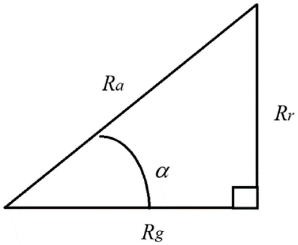
Markowitz uses expected income E and standard deviation σ to represent the income and risk of a portfolio. Similarly, we use Rg and Rr to represent the return and risk of a portfolio. Rr is defined in the following formula:
where Ra=1+E. Assuming that the geometric mean return of any portfolio is equivalent to the geometric mean return of a coin toss bet with an equal probability of gain or loss, then
Hg = logRg = 0.5log(Ra−Rr)+0.5log(Ra+Rr) .
Let sinα=Rr/Ra ϵ[0,1], which represents the bankruptcy risk better. When sinα is close to 1, the investment may go bankrupt (see Figure 3.9).
Figure 14.
Relationship between relative risk sinα and Rr, Ra, and Rg.
We call the pair (P, R) the investment channel, where P=(P1, P2, ... PM) is the future price vector, R=(Rik) is the return matrix, and the set of all possible investment ratio vectors is qC. Then, the capacity of the investment channel (abbreviated as investment capacity) is defined as
where q*= q*(R, P) is the optimal investment ratio.
For example, for a typical coin toss bet (with equal probabilities of winning and losing, and r0=0), q*=E/(r1r2), the investment capacity is:
Since 1/(1–x)=1+x+x2+…≈1+x, when E/Rr<<1, there is an approximate formula:
In comparison with the Gaussian channel capacity formula for communication:
we can see that the investment capacity formula is very similar to the Gaussian channel capacity formula. This similarity means that investment needs to reduce risk, just as communication needs to reduce noise.
4.3.4. Information Value Formula Based on Capital Growth Entropy
Weaver, who co-authored the book "A Mathematical Theory of Communication" [30] with Shannon, proposed three communication levels related to Shannon' 's information, semantic information, and information value.
According to the common usage of "information value", information value mentioned in the academic community does not refer to the value of information on markets but to the utility or utility increment generated by information. We define the information value as the increment of capital growth entropy [59].
Assume that the prior probability distribution of different returns is P(x), and the return matrix is (Rik), then the expected capital growth entropy is Hg(X). The optimal investment ratio vector q* is q*=q*(P(x),(Rik)). When the probability distribution of the predicted return becomes P(x|θj), the capital growth entropy becomes
The optimal investment ratio becomes q**=q**(P(x|θj), (Rik)). We define the increment of the capital growth entropy obtained after the semantic KL information I(X; θj) is provided as the information value (i.e., the average information value):
It can be seen that V(X; θj) and I(X; θj) have similar structures. For the above formula, when xi is determined to occur, the information value of yj becomes
Information value also needs to be verified by facts; wrong predictions may bring negative information value.
4.3.5. Comparison with Arrow's Information Value Formula
The utility function defined by Arrow is [56]:
where U(qiRi) is the utility obtained by the investor when the i-th return occurs.
Under the restriction of ∑i qi=1, qi=Pi(i=1,2,…) maximizes U so that
After receiving the information, the investor knows which income will occur and thus invests all his funds in it. Hence, there is
The information value is defined as the difference in utility between investment with and without information and is equal to Shannon entropy, that is
The optimal investment ratio obtained from the above formula is inconsistent with the Kelley formula and the conclusion of the author of this article. For example, according to the Kelley formula, the optimal ratio is 25% for the coin toss bet above. The compound interest is 0.061%, and the investment capacity is 0.084<<1 bit.
According to Arrow's theory, how does one bet? Should one bet 50% on each of the profit and loss?
Arrow seems to confuse the k-th security with the i-th return. He uses U(qiRi)=log(qiRi), while the author uses
Arrow does not consider the non-bet proportion q0, nor the paid proportion 1–q0–qk. The utility calculated in this way is puzzling.
Cover and Thomas inherited Arrow's method and concluded that when there is information, the optimal investment doubling rate increment equals Shannon MI [57] (see Section 6.2). Their conclusion has the same problem.
4.4. Information, Entropy, and Free Energy in Thermodynamic Systems
To clarify the relationship between information and free energy in physics, we discuss information, entropy, and free energy in thermodynamic systems.
According to Stirling's formula, lnN! = NlnN − N (when N→∞), there is a simple connection between Boltzmann entropy and Shannon entropy [60]:
where S' is entropy, k is the Boltzmann constant, xi is the i-th microscopic state, N is the number of molecules, and T is the absolute temperature, which equals a molecule's average translational kinetic energy. P(xi|T) represents the probability density of molecules in state xi at temperature T. The Boltzmann distribution is:
where Z is the partition function.
Considering the information between temperature and molecular energy, we use xi as energy ei. Let Gi denote the number of microscopic states with energy ei and G denote the number of all states. Then P(xi) = Gi/G is the prior probability of xi. So, Equation (58) becomes:
Under the energy constraint, when the system reaches equilibrium, Equation (59) becomes:
Now, we can interpret exp[−ei/(kT)] as the truth function T(θj|x), Z as the logical probability T(θj), and Equation (61) as the semantic Bayesian formula.
S and S' differ by a constant c (which does not change with temperature). There is S’=S+c, c=∑i P(xi)lnGi. If c is ignored, there is lnG=H(X)+c=H(X), and
Consider a local non-equilibrium system. Different regions yj(j = 1, 2, …) of the system have different temperatures Tj(j = 1, 2, …), so we have
Since P(yj)=Nj/N, we can get:
This formula shows the relationship between Shannon MI and physical entropy. It shows that the physical entropy S is similar to the posterior entropy H(X|Y) of x. The above formula shows that the Maximum Entropy (ME) law in physics can be equivalently expressed as the minimum MI law.
According to (47) and (48), when the local equilibrium is reached, there is
The above formula shows that for a local equilibrium system, the minimum Shannon MI can be expressed by the semantic MI formula.
Helmholtz's free energy formula is:
F=E-TS,
where F is free energy, and E is the system's internal energy. When the internal energy and temperature remain unchanged, the increase in free energy is
Comparing the above equation with Equations (63) and (64), we can find that Shannon MI is like the increase in free energy; semantic MI is like the increase in local equilibrium systems, which is smaller than Shannon MI, just as work is smaller than free energy. We can also regard kNT and kNTj as the unit information values [5], so the increase in free energy is similar to the increase in information value.
5. The G Theory for Machine Learning
5.1. Basic Methods of Machine Learning: Learning Functions and Optimization Criteria
The most basic machine learning method is:
- First, we use samples or sample distributions to train the learning functions with a specific criterion, such as maximum likelihood or RLS criterion;
- Then, we make probability predictions or classifications utilizing the learning function with minimum distortion, minimum loss, or maximum likelihood criteria.
When learning, we generally use maximum likelihood or RLS criteria; the criteria may differ for different tasks when classifying. For prediction tasks where information is important, we generally use maximum likelihood and RLS criteria. To judge whether a person is guilty or not, where correctness is essential, we may use the minimum distortion (or loss) criterion. The maximum semantic information criterion is equivalent to the maximum likelihood criterion, similar to the RLS criterion. Compared with the minimum distortion criterion, the maximum semantic information criterion can reduce the underreporting of small probability events.
We generally do not use P(x|yj) to train P(x|θj), because if P(x) changes, the originally trained P(x|θj) will become invalid. Using parameterized transition probability function P(θj|x) as a learning function is unaffected by P(x) changes. However, using P(θj|x) as a learning function also has essential defects. When category n >2, it is difficult to construct P(θj|x)(j=1,2,…) because of the normalization restriction, that is, ∑j P(θj|x)=1 (for each x). As we will see below, there is no restriction when using truth or membership functions as learning functions.
5.2. For Multi-Label Learning and Classification
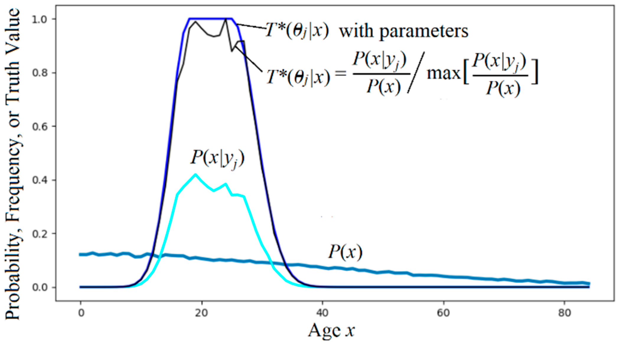
Consider multi-label learning, a supervised learning task. From the sample {(xk, yk), k = 1,2,…, N}, we can get the sample distribution P(x, y). Then, use formula (16) or (18) for the optimized truth functions.
Assume that a truth function is a Gaussian function, there should be:
So, we can use the expectation and standard deviation of P(x|yj)/P(x) or P(yj|x) as the expectation and standard deviation of T(θj|x). If the truth function is like a dam cross-section, we can get it through some transformation.
Figure 15.
Using prior and posterior distributions P(x) and P(x|yj) to obtain the optimized truth function T*(θj|x). For details, see Appendix B in [8].
Figure 15.
Using prior and posterior distributions P(x) and P(x|yj) to obtain the optimized truth function T*(θj|x). For details, see Appendix B in [8].
If we only know P(yj|x) but not P(x), we can assume that P(x) is equally probable, that is, P(x)=1/|U|, and then optimize the membership function using the following formula:
For multi-label classification, we can use the classifier:
If the distortion criterion is used, we can use –log T(θj|x) as the distortion function or replace I(X; θj) with T(θj|x).
The popular binary relevance method (Binary Relevance [61]) converts an n-label learning task into an n-pair label learning task. In comparison, the channel matching method is much simpler.
5.3. Maximum MI Classification for Unseen Instances
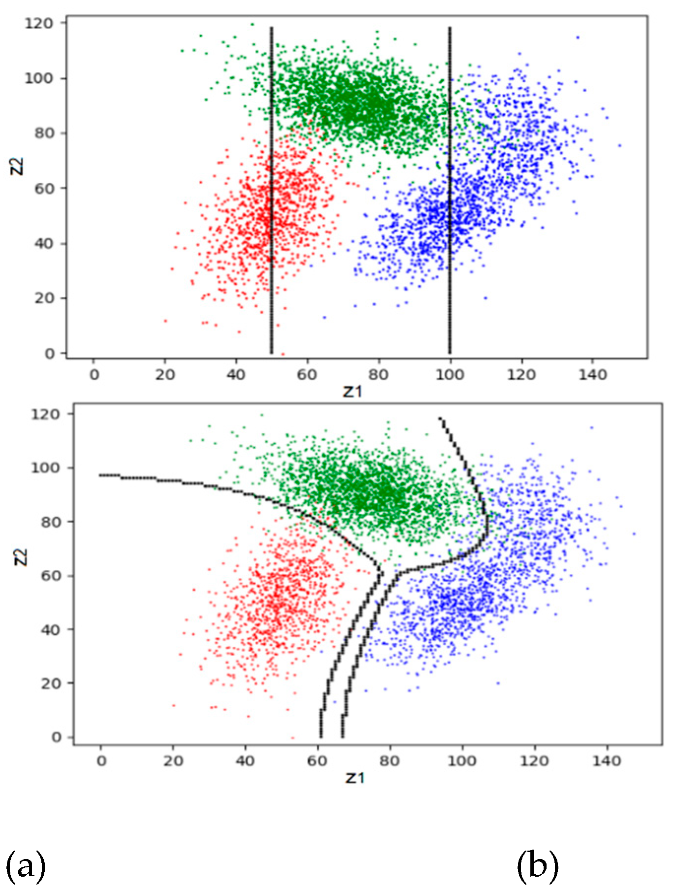
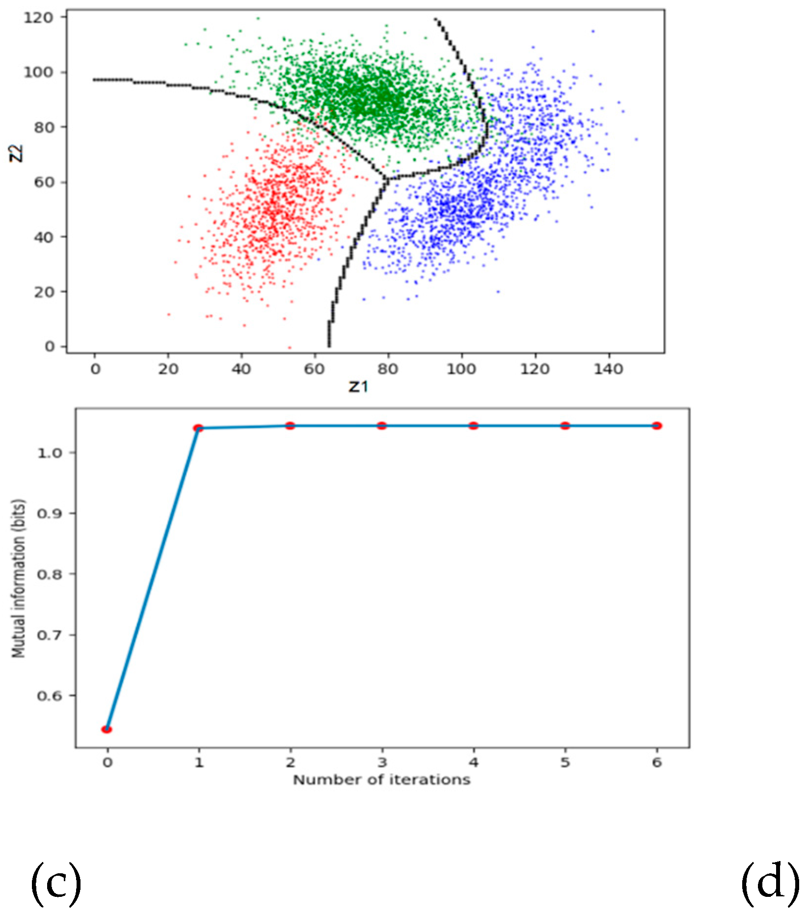
This type of classification belongs to semi-supervised learning. We take the medical test and the signal detection as examples (see Figure 16).
Figure 5.
Illustrating the medical test and the signal detection. We choose yj according to z∈Cj. The task is to find the dividing point z' that results in MaxMI between X and Y.
Figure 5.
Illustrating the medical test and the signal detection. We choose yj according to z∈Cj. The task is to find the dividing point z' that results in MaxMI between X and Y.
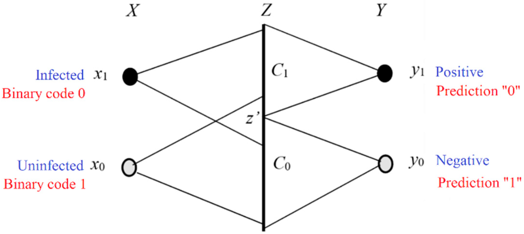
The following algorithm is not limited to binary classifications. Let Cj be a subset of C and yj = f(z|z∈Cj); hence S={C1, C2, …} is a partition of C. Our task is to find the optimized S, which is
First, we initiate a partition. Then we do the following iterations.
Matching I: Let the semantic channel match the Shannon channel and set the reward function. First, for given S, we obtain the Shannon channel:
Then we obtain the semantic channel T(y|x) from the Shannon channel and T(θj) (or mθ(x,y) = m(x, y)). Then we have I(xi; θj). For given z, we have conditional information as the reward function:
Matching II: Let the Shannon channel match the semantic channel by the classifier:
Repeat Matching I and Matching II until S does not change. Then, the convergent S is S* we seek. The author explained the convergence with the R(G) function (see Section 3.3 in [13]).
Figure 6 shows an example. The detailed data can be found in Section 4.2 of [13]. The two lines in Figure 6a represent the initial partition. Figure 6d shows that the convergence is very fast.
Figure 7.
The maximum MI classification. (a) A very bad initial partition; (b) after the first iteration; (c) after the second iteration; (d) the MI changes with the iteration number.
Figure 7.
The maximum MI classification. (a) A very bad initial partition; (b) after the first iteration; (c) after the second iteration; (d) the MI changes with the iteration number.
However, this method is unsuitable for maximum MI classification in high-dimensional space. We need to combine neural network methods to explore more effective approaches.
5.4. Explanation and Improvement of the EM Algorithm for Mixed Models
The EM algorithm [45,62,63] is usually used for mixed models or clustering, an unsupervised learning method.
We know that P(x)=∑j P(yj)P(x|yj). Given a sample distribution P(x), we use Pθ(x)=∑j P(yj)P(x|θj) to approximate P(x) so that the relative entropy or KL divergence KL(P‖Pθ) is close to 0. P(y) is the probability distribution of the latent variable to be sought.
The EM algorithm first presets P(x|θj) and P(yj), j = 1, 2, …, n. E-step obtains:
Then, in the M-step, the log-likelihood of the complete data (usually represented by Q) is maximized. The M-step can be divided into two steps: M1-step for
and M2-step for
which optimizes the likelihood function. For Gaussian mixture models, we can use the expectation and standard deviation of P(x)P(yj|x)/P+1(yj) as the expectation and standard deviation of P(x|θj+1).
From the perspective of the G theory, the M2-step is to make the semantic channel match the Shannon channel, the E-step is to make the Shannon channel match the semantic channel, and the M1-step is to make the destination P(y) match the source P(x). Repeating the above three steps can make the mixture model converge. The converged P(y) is the required probability distribution of the latent variable. According to the derivation process of the R(G) function, the E-step and M1-step minimize the information difference R–G; the M-step maximizes the semantic MI. Therefore, the optimization criterion used by the EM algorithm is the MIE criterion.
However, there are two problems with the above method to find the latent variable: 1) P(y) may converge slowly; 2) If the likelihood functions are also fixed, how do we solve P(y)?
Based on the R(G) function analysis, the author improved the EM algorithm to the EnM algorithm [64]. The EnM algorithm includes the E-step for P(y|x), n-step for P(y), and M-step for P(x|θj)(j=1,2,…). The n-step repeats the E-step and M1-step in the EM algorithm n times so that P+1(y) ≈ P(y). The EnM algorithm also uses the MIE criterion. The n-step can speed up the solution of P(y). M2-step only optimizes the likelihood functions. Because P(yj)/P+1(yj) is approximately equal to 1, we can use the following formula to optimize the model parameters:
Without n-step, there will be P(yj) ≠ P+1(yj), and ∑ i P(xi)P(x|θj)/Pθ(xi) ≠ 1. When solving the mixed model, we can choose a smaller n, such as n=3. When solving P(y) specifically, we can select a larger n until P(y) converges. When n=1, the EnM algorithm becomes the EM algorithm.
The following mathematical formula proves that the EnM algorithm converges. After the M-step, the Shannon MI becomes:
We define:
Then, we can deduce that after E-step, there is
where KL(P||Pθ) is the relative entropy or KL divergence between P(x) and Pθ(x); the right KL divergence is:
It is close to 0 after the n-step.
Equation (81) can be used to prove that the EnM algorithm converges. Because the M-step maximizes G, and the E-step and the n-step minimize R–G and KL(PY +1)‖PY), H(P‖Pθ) can be close to 0. We can also use the above method to prove that the EM algorithm converges.
In most cases, the EnM algorithm performs better than the EM algorithm [64], especially when P(y) is hard to converge.
Some researchers believe that EM makes the mixture model converge because the complete data log-likelihood Q = –H(X,Yθ) continues to increase [39], or negative free energy F′= H(Y)+Q continues to increase [45]. However, we can easily find counterexamples where R–G continues to decrease, but Q and F′ do not necessarily continue to increase. Figure 18 shows the example used by Neal and Hinton [45], but the mixture proportion in the true model is changed from 0.3:0.7 to 0.7:0.3.
Figure 18.
The convergent process of the mixture model from Neal and Hinton [45]. The mixture proportion is changed from 0.7:0.3 to 0.3:0.7. (a) The iteration starts; (b) the iteration converges; (c) the iteration process. P(x, θj)=P(yj)P(x|θj) (j=0, 1).
Figure 18.
The convergent process of the mixture model from Neal and Hinton [45]. The mixture proportion is changed from 0.7:0.3 to 0.3:0.7. (a) The iteration starts; (b) the iteration converges; (c) the iteration process. P(x, θj)=P(yj)P(x|θj) (j=0, 1).

This experiment shows that the decrease in R–G, not the increase in Q or F', is the reason for the convergence of the mixture model.
The free energy of the true mixture model (with true parameters) is the Shannon conditional entropy H(X|Y). If the standard deviation of the true mixture components is large, H(X|Y) is also large. If the initial standard deviation is small, F is small initially. After the mixture model converges, F must be close to H(X|Y). Therefore, F increases (i.e., F' decreases) during the convergence process. Many experiments [25,64] have shown that this is indeed the case.
Equation (77) can also explain pre-training in deep learning, where we need to maximize the model's predictive ability and minimize the information difference R–G (or compress data).
5.5. Semantic Variational Bayes: A Simple Method for Solving Hidden Variables
Given P(x) and constraints P(x|θj), j=1,2,…, we need to solve P(y) that produces P(x)=∑j P(yj)P(x|θj). P(y) is the probability distribution of the latent variable y, sometimes called the latent variable. The popular method is the Variational Bayes method (VB for short) [65]. This method originated from the article by Hinton and Camp [44]. It was further discussed and applied in the articles by Neal and Hinton [45], Beal [66], and Koller [67] (ch.11). Gottwald and Braun's article "Two Free Energy and the Bayesian Revolution" [68] discusses the relationship between the MFE principle and ME principle in detail.
VB uses P(y) (usually written as g(y)) as a variation to minimize the following function:
It is equal to the semantic posterior entropy H(X|Yθ) of X. The smaller F is, the larger the semantic MI I(X; Y))=H(X)–H(X|Yθ) is.
It is easy to prove that when the semantic channel matches the Shannon channel, that is, T(θj|x)∝P(yj|x) or P(x|θj)=P(x|yj) (j=1,2,…), F is minimized and the semantic MI is maximized. This can optimize the prediction model P(x|θj)(j=1,2,…), but it cannot optimize P(y). For optimizing P(y), the mean field approximation [45,65] is usually used; that is, P(y|x) instead of P(y) is used as the variation. Only one P(yj|x) is optimized at a time, and the other P(yk|x) (k≠j) remains unchanged. Minimizing F in this way is actually maximizing the log-likelihood of x or minimizing KL(P||Pθ). In this way, optimizing P(y|x) also indirectly optimizes P(y).
Unfortunately, when optimizing P(y) and P(y|x), F may not decrease (see Figure 18). So, VB is good as a tool and is imperfect as a theory.
Fortunately, it is easier to solve P(y|x) and P(y) using the MID iteration in solving R(D) and R(G) functions. The MID iteration plus LBI for optimizing the prediction model is the Semantic Variational Bayes' method (abbreviated as SVB) [30]. It uses the MIE criterion.
When the constraint changes from likelihood functions to truth functions or similarity functions, P(yj|xi) in the MID iteration formula is changed from
to
From P(x) and the new P(y|x), we can get the new P(y). Repeating the formulas for P(y|x) and P(y) will lead to convergence of P(y). Using s allows us to tighten the constraints for increasing R and G. Choosing proper s enables us to balance between maximizing semantic information and maximizing information efficiency.
The main tasks of SVB and VB are the same: using variational methods to solve latent variables based on observed data and constraints. The differences are:
- Criteria: In the definition of VB, it adopts the MFE (i.e., minimum semantic posterior entropy) criterion, whereas, for solving P(y), it uses P(y|x) as the variation, actually uses the maximum likelihood criterion that makes the mixture model converge. In contrast, SVB uses the MID criterion, equal to the maximum likelihood criterion (optimizing model parameters) plus the ME criterion.
- Variational method: VB only uses P(y) or P(y|x) as the variation, while SVB alternatively uses P(y|x) and P(y) as the variation.
- Computational complexity: VB uses logarithmic and exponential functions to solve P(y|x) [65]; the calculation of P(y|x) in SVB is relatively simple (for the same task, i.e., when s=1).
- Constraints: VB only uses likelihood functions as constraint functions. In contrast, SVB allows using various learning functions (including likelihood, truth, membership, similarity, and distortion functions) as constraints. In addition, SVB can use the parameter s to enhance constraints.
Because SVB is more compatible with the maximum likelihood criterion and the ME principle, it should be more suitable for many occasions in machine learning. However, because it does not consider the probability of parameters, it may not be as applicable as VB in some occasions. See [30] for more details of SVB.
5.6. Bayesian Confirmation and Causal Confirmation
Logical empiricism was opposed by Popper's falsificationism [19,20], so it turned to confirmation (i.e., Bayesian confirmation) instead of induction or positivism [69,70]. Bayesian confirmation was previously a field of concern for researchers in the philosophy of science [61,72], and now many researchers in natural sciences have also begun to study it [26,73,74]. The reason is that uncertain reasoning requires major premises, which need to be confirmed.
The main reasons why researchers have different views on Bayesian confirmation are:
- There are no suitable mathematical tools; for example, statistical and logical probabilities are not well distinguished.
- Many people do not distinguish between the confirmation of the relationship (i.e. →) in the major premise y→x and the confirmation of the consequent (i.e., x occurs);
- No confirmation measure can reasonably clarify the Raven Paradox.
To clarify the Raven paradox, the author wrote the article "Channels' confirmation and predictions' confirmation: from medical tests to the Raven paradox" [26].
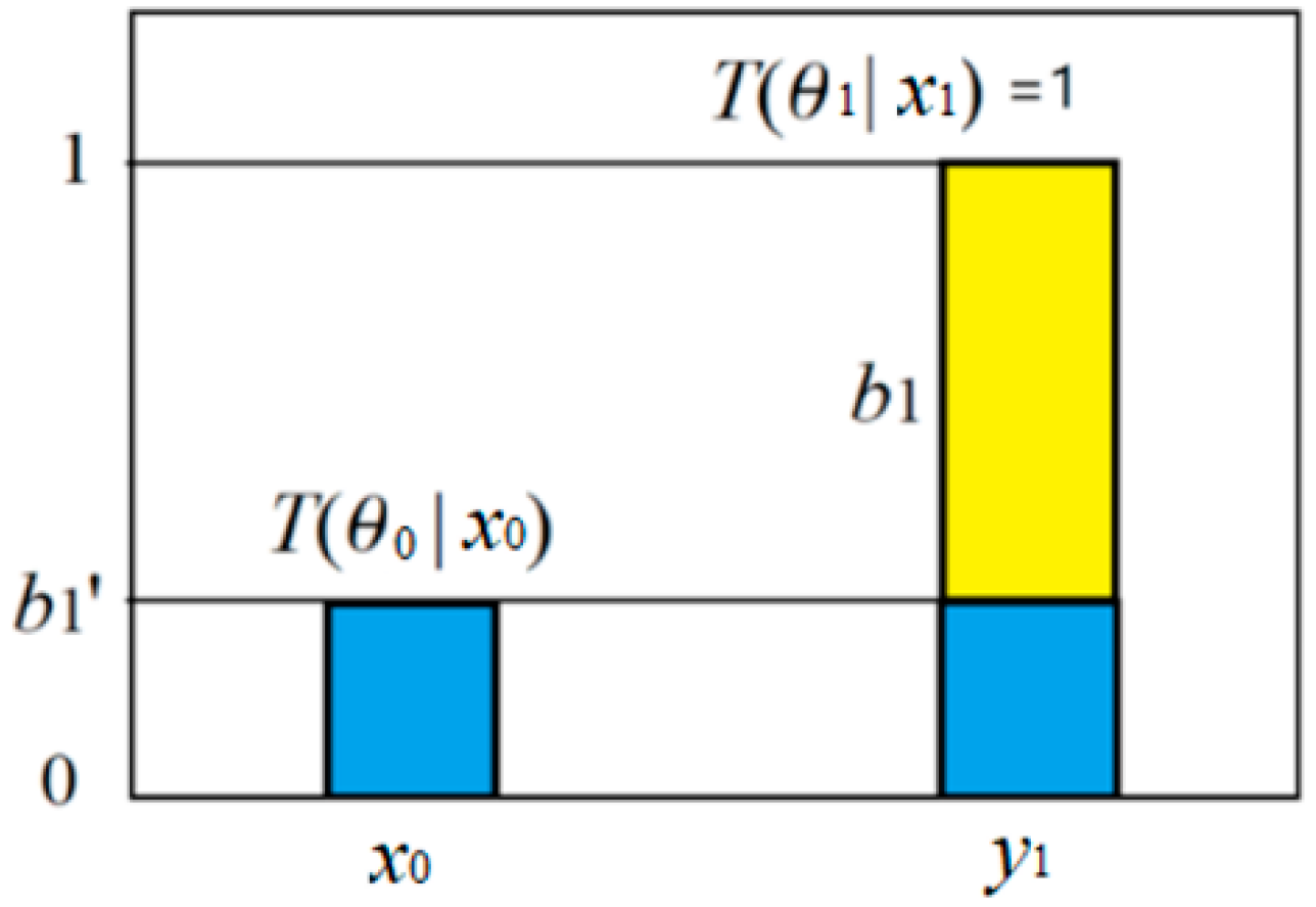
In the author's opinion, the task of Bayesian confirmation is to evaluate the support of the sample distribution for the major premise. For example, for the medical test (see Figure 16), a major premise is "If a person tests positive (y1), then he is infected (x1)", abbreviated as y1→x1. For a channel's confirmation, a truth (or membership) function can be viewed as a combination of a clear truth function T(y1|x)∈{0,1} and a tautology's truth function (always 1):
T(θ1|x) = b1T(y1|x) + b1’.
A tautology's proportion b1' is the degree of disbelief. The credibility is b1, and its relationship with b1’ is b1’=1–|b1|. See Figure 19.
Figure 19.
A truth function includes a believable proportion b1 and unbelievable proportion b1' = 1 − |b1|.
Figure 19.
A truth function includes a believable proportion b1 and unbelievable proportion b1' = 1 − |b1|.
We change b1 to maximize the semantic KL information I(X; θ1), the optimized b1, denoted as b1*, is the confirmation degree:
where R+=P(y1|xi)/P(y1|x0) is the positive likelihood ratio, indicating the reliability of the test- positive. This conclusion is compatible with medical test theory.
Considering the prediction confirmation degree, we assume that P(x|θ1) is a combination of the 0-1 part and the equal probability part. The ratio of the 0-1 part is the prediction credibility, and the optimized credibility is the prediction confirmation degree:
where a is the number of positive examples, and c is the number of negative examples.
Both confirmation degrees can be used for probability predictions, that is, to calculate P(x|θ1)[26].
Hemple proposed a confirmation paradox, namely the raven paradox [61]. According to the equivalence condition in classical logic, "if x is a raven, then x is black" (Rule 1) is equivalent to "if x is not black, then x is not a raven" (Rule 2). According to this, white chalk supports Rule 2; therefore, it also supports Rule 1. However, according to common sense, a black crow supports Rule 1, and a non-black Raven opposes Rule 1; something that is not a Raven, such as a black cat or a white chalk, is irrelevant to Rule 1. Therefore, there is a paradox between the equivalence condition and common sense. Using the confirmation measure c1*, we can be sure that common sense is correct and the equivalence condition is wrong (for fuzzy major premises), thus eliminating the Raven paradox. However, other confirmation measures cannot eliminate the Raven paradox [26].
Causal probability is used in causal inference theory [75]:
It indicates the necessity of the cause x1 replacing x0 to lead to the result y1. Where P(y1|x)=P(y1|do(x)) is the posterior probability of y1 caused by intervention x. The author uses the semantic information method to obtain the channel causal confirmation degree [27]:
It is compatible with the above causal probability but can express negative causal relationships, such as the necessity of vaccines inhibiting infection.
5.7. Emerging and Potential Applications
1) About self-supervised Learning
Applications of estimated MI have emerged in the field of self-supervised learning. The estimated MI is a special case of semantic MI. Both MINE proposed by Belghazi et al. [34] and InfoNCE proposed by Oord et al. [35] use estimated MI.
MINE and InfoNCE are essentially the same as the semantic information methods. Their common features are:
- The membership function T(θj|x) or similarity function S(x, yj) proportional to P(yj|x) is used as the learning function. Its maximum value is generally 1, and its average is the partition function Zj.
- The estimated information or semantic information between x and yj is log[T(θj|x)/Zj] or log[S(x, yj)/Zj].
- The statistical probability distribution P(x, y) is still used when calculating the average information.
However, many researchers are still unclear about the relationship between estimated MI and Shannon MI. The G theory's R(G) function can help readers understand this relationship.
2) About Reinforcement Learning
Goal-oriented information introduced in Section 4.2 can be used as a reward for reinforcement learning. Assuming that the probability distribution of x in state sk is P(x|ak–1), which becomes P(x|ak) in state sk+1. The reward of ak is:
Reinforcement learning is to find the optimal action sequence a1, a2, …, so that the sum of rewards r1+r2+… is maximized.
Like constraint control, reinforcement learning also needs the trade-off between maximum purposefulness and minimum control cost. The R(G) function should be helpful.
3) About the Truth function and Fuzzy Logic for Neural Networks
When we use the truth, distortion, or similarity function as the weight parameters of the neural network, the neural network contains semantic channels. Then, we can use semantic information methods to optimize the neural network. Using the truth function T(θj|x) as weight is better than using the parameterized inverse probability function P(θj|x) because there is no normalization restriction when using truth functions.
However, unlike the clustering of points on the plane, a point becomes an image for the clustering of graphics, and the similarity function between images needs different methods. A common method is to regard an image as a vector and use cosine similarity between vectors. However, cosine similarity may have negative values, which require activation functions and biases to make necessary conversions. Combining existing neural network methods and channel-matching algorithms needs further exploration.
Fuzzy logic, especially fuzzy logic compatible with Boolean algebra, seems to be useful in neural networks; for example, the activation function Relu(a–b) = max(0, a–b) commonly used in neural networks is the logical difference operation f(a)=max(0, a–b) used in the author's color vision mechanism model [76,77,78]. Truth functions, fuzzy logic, and the semantic information method used in neural networks should make neural networks easier to understand.
4) Explaining Data Compression in Deep Learning
To explain the success of deep neural networks such as AutoEncoders [36] and Deep Belief Networks [79], Tishby et al. [39] proposed the information bottleneck explanation, arguing that when optimizing deep neural networks, we maximize the Shannon MI between some layers and minimize the Shannon MI between other layers. However, from the perspective of the R(G) function, each coding layer of the Autoencoder needs to maximize the semantic MI G and minimize the Shannon MI R; pre-training is to let the semantic channel match the Shannon channel so that G≈R and KL(P||Pθ)≈0 (as if for mixture models to converge). Fine-tuning increases R and G at the same time by increasing s (making the partition boundaries steeper).
6. Discussion and Summary
6.1. Why Is the G Theory a Generalization of Shannon's Information Theory?
First, the semantic information G measure is a generalization of Shannon's information measure. The methods are:
- In addition to the probability prediction P(x|yj), the semantic probability prediction P(x|θj)=P(x)T(θj|x)/T(θj) is also used;
- The G measure also has coding meaning, which means the average code length saved by the semantic probability prediction.
Second, the semantic communication model is essentially the Shannon communication model; the difference is that it changes the distortion constraint to the semantic constraint, including semantic distortion constraint (for R(θ)), semantic information constraint (for the R(G) function) and the semantic information loss constraint (for electronic communication, see Section 3.2).
Third, the G theory adheres to Shannon's concept of information: information is reduced uncertainty.
6.2. What Is Information?
What is information? This question has many answers [82]. According to Shannon's definition, information is uncertainty reduced. Shannon information is the uncertainty reduced due to the increase of probability, while semantic information is the uncertainty reduced due to the narrowing of concepts' extensions.
From a common-sense perspective, information refers to something previously unknown or uncertain, which encompasses:
Information from natural language: information provided by answers to interrogative sentences (e.g., sentences with "Who?", "What?", "When?", "Where?", "Why?", "How?", or "Is this?").
Perceptual or observational information: information obtained from material properties or observed phenomena.
Symbolic information: information conveyed by various symbols like road signs, traffic lights, and battery polarity symbols.
Quantitative indicators' information: information provided by data such as time, temperature, rainfall, stock market indices, and inflation rates.
Associated information: information derived from event associations, such as the crowing of a rooster signaling dawn and a positive medical test indicating disease.
Items 2, 3, and 4 can also be viewed as answers to questions in item 1, thus providing information. These forms of information involve concept extensions and truth-falsehood considerations and should be semantic information. Associated information in item 5 can be measured using Shannon's or the semantic information formula. When probability predictions are inaccurate (i.e., P(x|θj)≠P(x|yj)), the semantic information formula is more appropriate. Thus, the G theory is consistent with the concept of information in everyday life.
In computer science, information is often defined as useful, structured data. What qualifies as "useful"? This utility arises because the data can answer various questions or provide associated information. Therefore, the definition of information in data science also ties back to reduced uncertainty and narrowed concept extensions.
6.3. Relationships and Differences Between the G Theory and Other Demantic Information Theories
6.3.1. Carnap and Bar-Hillel's Semantic Information Theory
The semantic information measure of Carnap and Bar-Hillel is [3]:
Ip=log(1/mp], (
where Ip is the semantic information provided by the proposition set p, and mp is the logical probability of p. This formula reflects Popper's idea that smaller logical probabilities convey more information. However, as Popper noted, this idea requires the hypothesis to withstand factual testing. The above formula does not account for such tests, implying that correct and incorrect hypotheses provide the same information.
Additionally, the G theory differs in calculating logical probability with statistical probability, unlike Carnap and Bar-Hillel's approach.
6.3.2. Dretske's Knowledge and Information Theory:
Dretske [9] emphasized the relationship between information and knowledge, viewing information as content tied to facts and knowledge acquisition. Though he did not propose a specific formula, his ideas about information quantification include:
- The information must correspond to facts and eliminate all other possibilities.
- The amount of information relates to the extent of uncertainty eliminated.
- Information used to gain knowledge must be true and accurate.
The G theory aligns with these principles by providing semantic information formulas and mathematically implementing Dretske's concepts.
6.3.3. Florida's Strong Semantic Information Theory:
Florida's theory [12] emphasizes:
- The information must contain semantic content and be consistent with reality:
- False or misleading information cannot qualify as true information.
Floridi elaborated on Dretske's ideas and introduced a strong semantic information formula. However, this formula is more complex and less effective at reflecting factual testing compared to the G theory. For instance, Floridi's approach ensures tautologies and contradictions yield zero information but fails to penalize false predictions with negative information.
6.3.4. Other Semantic Information Theories:
In addition to the semantic information theories mentioned above, other well-known ones include the theory based on fuzzy entropy proposed by Zhong [11] and the theory based on synonymous mapping proposed by Niu and Zhang [17]. Zhong advocated the combination of information science and artificial intelligence, which had a great influence on China's semantic information theory research. He employed fuzzy entropy to define the semantic information measure. However, this approach yielded identical maximum values (1 bit) for both true and false sentences [11], which is counterintuitive. Other people's semantic information measures using DeLuca and Termini's fuzzy entropy also encounter similar problems.
Other authors who discussed semantic information measure and semantic entropy include D'Alfonso [84], Basu et al. [85], and Melamed [86]. These authors improved semantic information measures by improving Carnap and Bar-Hillel's logical probability. The semantic entropy used is mainly in the form of Shannon entropy. The semantic entropy H(Yθ) in G theory differs from these semantic entropies. It contains statistical and logical probabilities and reflects the average code length of lossless coding (see Section 2.3).
Niu and Zhang [17] and Guo et al. [87] proposed the semantic information rate-distortion function Rs(D), where Rs represents minimum semantic information. In contrast, R(G) in the G theory still represents the minimum Shannon MI, reflecting the lower limit of data compression. Why do we minimize semantic MI? The reason seems to be that researchers want to establish a semantic information theory parallel to Shannon's information theory. Liu et al. [88] used the dual-constrained rate-distortion function R(Ds, Dx); Guo et al. [87] also used R(Ds, Dx), which is meaningful. In contrast, G in R(G) already contains dual constraints because G means fidelity and semantic information.
6.4. Relationship Between the G Theory and Kolmogorov Complexity Theory
Kolmogorov [92] defined the complexity of a string of data as the shortest code length under the requirement of lossless recovery. The information provided by knowledge is defined as the complexity reduced by knowledge. Shannon's information measured can be understood as the average information, while Kolmgorov's information is the information provided by knowledge about a data string. Shannon's information theory does not consider the complexity of individual data, while Kolmogorov's theory does not consider statistical averages. It can be said that Kolmogorov defined the amount of information in microdata, while Shannon provided the mutual information formula for measuring the information of macrodata. The two theories are complementary.
Because knowledge includes the extensions of concepts and the logical relationships between concepts, as well as the correlations (including causality) between things, the information defined by Kolmogorov contains semantic information. However, Kolmogorov did not provide a specific formula for measuring information. The G theory provides semantic Bayesian prediction, semantic information measure, and the R(G) function, which should supplement the above two theories.
The relationship between the G theory and Kolmogorov complexity needs further study.
6.5. Comparison of the MIE Principle and the MFE Principle
Friston proposed the MFE principle, which he believed was a universal principle organisms use to perceive the world and adapt to the environment (including transforming the environment). The core mathematical method he uses is VB. A similar principle used by the G theory is the MIE principle.
The main differences between the two are:
- The G theory regards Shannon's MI I(X; Y) as free energy, while Friston's theory regards the semantic posterior entropy H(X|Yθ) as free energy.
- The methods for finding the latent variable P(y) and the Shannon channel P(y|x) are different. Friston uses VB, and the G theory uses SVB.
When optimizing the prediction model P(x|θj)(j=1,2,…), the two are consistent; when optimizing P(y) and P(y|x), the results of the two are similar, but the methods are different. SVB is simpler. The reason why the results are similar is that VB uses the mean-field approximation when optimizing P(y|x), which is equivalent to using P(y|x) instead of P(y) as a variation and actually uses the MID criterion. So, the two results are almost the same. Figure 18 shows that in a mixture model's convergence process, information difference R–G instead of free energy F continuously decreases.
In physics, free energy is energy that can be used to do work; the more, the better. Why should it be minimized? In physics, there are two situations in which free energy is reduced. One is passive reduction because of the increase in entropy. The other reason is to save the consumed free energy while doing work. This is for considering thermal efficiency, which is a conditional reduction. Reducing the consumed free energy conforms to Jaynes' maximum entropy principle. Therefore, from a physics perspective, it is not easy to understand that one would actively minimize free energy.
MIE is like the maximum doing-work efficiency W/F when using free energy F to do work W. The MIE principle is easier to understand.
The author will discuss these two principles further in other articles.
6.6. Limitations and Areas That Need Exploration
The G theory is still a basic theory. It has limitations in many aspects, and many elements need improvement.
1) Semantics and Distortion of Complex Data
Truth functions can represent the semantic distortion of labels. However, it is difficult to express the semantics, semantic similarity, and semantic distortion of complex data (such as a sentence or an image). Many researchers have made valuable explorations [15,93]. The author's research is insufficient.
The semantic relationship between a word and many other words is also very complex. Innovations like Word2Vec [94,95] in deep learning have successfully modeled these relationships, paving the way for advancements like Transformer [96] and ChatGPT. Future work in the G theory should aim to integrate such developments to align with the progress in deep learning.
2) Feature Extraction
The features of images encapsulate most semantic information. There are many efficient feature extraction methods in deep learning, such as Convolutional Neural Networks and AutoEncoders. These methods are ahead of the G theory. Whether the G theory can be combined with these methods to obtain better results needs further exploration.
3) The Channel-matching Algorithm for Neural Networks
Establishing neural networks to enable mutual alignment of Shannon and semantic channels appears feasible. Current deep learning practices, relying on gradient descent and backpropagation, demand significant computational resources. If the channel matching algorithm can reduce reliance on these methods, it would save computational power and physical free energy.
4) Neural Networks Utilizing Fuzzy Logic
Using truth functions or their logarithms as network weights facilitates the application of fuzzy logic. The author previously used a fuzzy logic method compatible with Boolean algebra to set up a symmetrical color vision mechanism model: the 3-8 decoding model [76,77,78,79]. Combining the G theory with fuzzy logic and neural networks holds promise for further exploration.
5) Optimizing Economic Indicators and Forecasts:
Forecasting in weather, economics, and healthcare domains provides valuable semantic information. Traditional evaluation metrics, such as accuracy or average error, can now be enhanced by converting distortion into truth. Using truth functions to represent semantic information offers a novel method for evaluating and optimizing forecasts, which merits further exploration.
6.7. Conclusion
The G theory's validity is supported by its broad applications across multiple domains, particularly in solving problems related to semantic communication, semantic compression theory, multi-label learning, maximum mutual information classification, mixture models, latent variable resolution, Bayesian confirmation, constraint control, investment portfolios and information value. Particularly, the G theory allows us to utilize the existing coding methods for semantic communication. The crucial approach is to replace distortion constraints with semantic constraints, where the information rate-distortion function becomes the information rate-fidelity function.
However, the G theory's primary limitation lies in the semantic representation of complex data. In this regard, it has lagged behind the advancements in deep learning. Bridging this gap will require learning from and integrating insights from other studies and technologies.
Funding
This research received no external funding.
Informed Consent Statement
Not applicable.
Data Availability Statement
Not applicable.
Acknowledgments
The Author particularly thanks Viacheslav Kovtun. Without his encouragement, the Author would not have finished this review.
Conflicts of Interest
The Author declares no conflict of interest.
Appendix A. Abbreviations
| Abbreviation | Original text |
| EM | Expectation-Maximization |
| EnM | Expectation-n-Maximization |
| GPS | Global Positioning System |
| G theory | Semantic information G theory (G means generalization) |
| InfoNCE | Information Noise Contrast Estimation |
| KL | Kullback–Leibler |
| LBI | Logical Bayes' Inference |
| ME | Maximum Entropy |
| MI | Mutual Information |
| MIE | Maximum Information Efficiency |
| MID | Minimum Information Difference |
| MINE | Mutual Information Neural Estimation |
| SVB | Variational Byes |
| VB | Semantic Variational Byes |
References
- Shannon, C.E. A mathematical theory of communication. Bell Syst. Tech. J. 1948, 27, 379–423. [Google Scholar] [CrossRef]
- Weaver, W. Shannon, C.E., Weaver, W., Eds.; Recent contributions to the mathematical theory of communication. In The Mathematical Theory of Communication, 1st ed.; The University of Illinois Press: Urbana, IL, USA, 1963; pp. 93–117. [Google Scholar]
- Carnap, R.; Bar-Hillel, Y. An Outline of a Theory of Semantic Information; Tech. Rep. No. 247; Research Laboratory of Electronics, MIT: Cambridge, MA, USA, 1952. [Google Scholar]
- Lu, C. Shannon equations reform and applications. BUSEFAL 1990, 44, 45–52. Available online: https://www.listic.univ-smb.fr/production-scientifique/revue-busefal/version-electronique/ebusefal-44/ (accessed on 5 March 2019).
- Lu, C. A Generalized Information Theory; China Science and Technology University Press: Hefei, China, 1993; (in Chinese). ISBN 7-312-00501-2. [Google Scholar]
- Lu, C. Meanings of generalized entropy and generalized mutual information for coding. J. China Inst. Commun. 1994, 15, 37–44 (in Chinese). (in Chinese). [Google Scholar]
- Lu, C. A generalization of Shannon’s information theory. Int. J. Gen. Syst. 1999, 28, 453–490. [Google Scholar] [CrossRef]
- Lu, C. Semantic Information G Theory and Logical Bayesian Inference for Machine Learning. Information, 2019, 10, 261. [Google Scholar] [CrossRef]
- Dretske, F. Knowledge and the Flow of Information. The MIT Press: Cambridge, Massachusetts, 1981; ISBN 0-262-04063-8. [Google Scholar]
- Wu, W. General source and general entropy. Journal of Beijing University of Posts and Telecommunications, (in Chinese). 吴伟陵 [1]吴伟陵.广义信息源与广义熵[J].北京邮电大学学报, 1982, 5(1):29-41. 1982, 5, 29–41. [Google Scholar]
- Zhong, Y. A Theory of Semantic Information. Proceedings 2017, 1, 129. [Google Scholar] [CrossRef]
- Floridi, L. Outline of a theory of strongly semantic information. Minds and Machines, 2004, 14, 197–221. [Google Scholar] [CrossRef]
- Floridi, L. Semantic conceptions of information. In Stanford Encyclopedia of Philosophy; Stanford University: Stanford, CA, USA, 2005; Available online: http://seop.illc.uva.nl/entries/information-semantic/ (accessed on 17 June 2020).
- D’Alfonso, S. On Quantifying Semantic Information. Information 2011, 2, 61–101. [Google Scholar] [CrossRef]
- Xin, G.; Fan, P.; Letaief, K.B. Semantic Communication: A Survey of Its Theoretical Development. Entropy 2024, 26, 102. [Google Scholar] [CrossRef]
- Strinati, E.C.; Barbarossa, S. 6G networks: Beyond Shannon towards semantic and goal-oriented communications. Comput. Netw. 2021, 190, 107930. [Google Scholar] [CrossRef]
- Kai Niu, Ping Zhang. A mathematical theory of semantic communication. Journal on Communications 2024, 45, 8–59. [Google Scholar]
- Davidson, D. Truth and meaning. Synthese 1967, 3, 304–323. [Google Scholar] [CrossRef]
- Popper, K. Logik Der Forschung: Zur Erkenntnistheorie Der Modernen Naturwissenschaft; Springer: Vienna, Austria, 1935. [Google Scholar]
- Popper, K. Conjectures and Refutations, 1st ed.; Routledge: London and New York, 2002. [Google Scholar]
- Fisher, R.A. On the mathematical foundations of theoretical statistics. Philos. Trans. R. Soc. 1922, 222, 309–368. [Google Scholar]
- Zadeh, L.A. Fuzzy sets. Inf. Control 1965, 8, 338–353. [Google Scholar] [CrossRef]
- Zadeh, L.A. Probability measures of fuzzy events. J. Math. Anal. Appl. 1986, 23, 421–427. [Google Scholar] [CrossRef]
- Lu, C. The P–T probability framework for semantic communication, falsification, confirmation, and Bayesian reasoning. Philosophies 2020, 5, 25. [Google Scholar] [CrossRef]
- Lu, C. Reviewing evolution of learning functions and semantic information measures for understanding deep learning. Entropy 2023, 25, 802. [Google Scholar] [CrossRef]
- Lu, C. Channels’ confirmation and predictions’ confirmation: From the medical test to the raven paradox. Entropy 2020, 22, 384. Available online: https://www.mdpi.com/1099-4300/22/4/384. [CrossRef]
- Lu, C. Causal Confirmation Measures: From Simpson’s Paradox to COVID-19. Entropy 2023, 25, 143. [Google Scholar] [CrossRef]
- Lu, C. Using the Semantic Information G Measure to Explain and Extend Rate-Distortion Functions and Maximum Entropy Distributions. Entropy 2021, 23, 1050. [Google Scholar] [CrossRef] [PubMed]
- Lu, C. Semantic Information G Theory for Range Control with Tradeoff between Purposiveness and Efficiency, Available online:. Available online: https://arxiv.org/abs/2411.05789. (accessed on 1 January 2025).
- Lu, C. Semantic Variational Bayes Based on a Semantic Information Theory for Solving Latent Variables. Available online: https://doi.org/10.48550/arXiv.2408.13122 (accessed on 1 January 2025).
- Shannon, C.E. Coding theorems for a discrete source with a fidelity criterion. IRE Nat. Conv. Rec. 1959, 4, 142–163. [Google Scholar]
- Berger, T. Rate Distortion Theory; Prentice-Hall: Enklewood Cliffs, NJ, USA, 1971. [Google Scholar]
- Zhou, J.P. Fundamentals of information theory. 1983. (in Chinese). [Google Scholar]
- Belghazi, M.I.; Baratin, A.; Rajeswar, S.; Ozair, S.; Bengio, Y.; Courville, A.; Hjelm, R.D. MINE: Mutual information neural estimation. In Proceedings of the 35th International Conference on Machine Learning, Stockholm, Sweden, 10–15 July 2018; pp. 1–44. [Google Scholar] [CrossRef]
- Oord, A.V.D.; Li, Y.; Vinyals, O. Representation Learning with Contrastive Predictive Coding. Available online: https://arxiv.org/abs/1807.03748 (accessed on 10 January 2023).
- Hinton, G.E.; Salakhutdinov, R.R. Reducing the dimensionality of data with neural networks. Science 2006, 313, 504–507. [Google Scholar] [CrossRef]
- Hjelm, R.D.; Fedorov, A.; Lavoie-Marchildon, S.; Grewal, K.; Trischler, A.; Bengio, Y. Learning Deep Representations by Mutual Information Estimation and Maximization. Available online: https://arxiv.org/abs/1808.06670. (accessed on 22 December 2022).
- Tschannen, M.; Djolonga, J.; Rubenstein, P.K.; Gelly, S.; Luci, M. On Mutual Information Maximization for Representation Learning. Available online: https://arxiv.org/pdf/1907.13625.pdf (accessed on 23 February 2023).
- Tishby, N.; Zaslavsky, N. Deep learning and the information bottleneck principle. In Proceedings of the Information Theory Workshop (ITW), Jerusalem, Israel, 26 April–1 May 2015; pp. 1–5. [Google Scholar]
- Tarski, A. The semantic conception of truth: and the foundations of semantics. Philos. Phenomenol. Res. 1994, 4, 341–376. [Google Scholar] [CrossRef]
- Kolmogorov, A.N. Grundbegriffe der Wahrscheinlichkeitrechnung; Dover Publications: New York, NY, USA, 1950; Ergebnisse Der Mathematik (1933); translated as Foundations of Probability. [Google Scholar]
- von Mises, R. Probability, Statistics and Truth, 2nd ed.; George Allen and Unwin Ltd.: London, UK, 1957. [Google Scholar]
- Akaike, H. A new look at the statistical model identification. IEEE Trans. Autom. Control. 1974, 19, 716–723. [Google Scholar] [CrossRef]
- Geoffrey, E. Hinton and Drew van Camp. Keeping the neural networks simple by minimizing the description length of the weights. In Proceedings of COLT; pp. 5–13.
- Neal, R.; Hinton, G. Michael, I.J., Ed.; A view of the EM algorithm that justifies incremental, sparse, and other variants. In Learning in Graphical Models; MIT Press: Cambridge, MA, USA, 1999; pp. 355–368. [Google Scholar]
- Friston, K. The free-energy principle: a unified brain theory? Nat Rev Neurosci 2010, 11, 127–138. [Google Scholar] [CrossRef]
- Wang, P.Z. From the fuzzy statistics to the falling random subsets. In Advances in Fuzzy Sets, Possibility Theory and Applications; Wang, P.P., Ed.; Plenum Press: New York, NY, USA, 1983; pp. 81–96. [Google Scholar]
- Wang, P.Z. Fuzzy Sets and Falling Shadows of Random Set; Beijing Normal University Press: Beijing, China, 1985. (In Chinese) [Google Scholar]
- Farsad, N.; Rao, M.; Goldsmith, A. Deep learning for joint source-channel coding of text. In Proceedings of the 2018 IEEE International Conference on Acoustics, Speech and Signal Processing (ICASSP), Calgary, AB, Canada, 15–20 April 2018; IEEE: New York, NY, USA, 2018; pp. 2326–2330. [Google Scholar]
- Güler, B.; Yener, A.; Swami, A. The semantic communication game. IEEE Trans. Cogn. Commun. Netw. 2018, 4, 787–802. [Google Scholar] [CrossRef]
- Papineni, K.; Roukos, S.; Ward, T.; Zhu, W.J. Bleu: A method for automatic evaluation of machine translation. In Proceedings of the 40th Annual Meeting of the Association for Computational Linguistics, Philadelphia, PA, USA, 6–12 July 2002; pp. 311–318. [Google Scholar]
- Xie, H.; Qin, Z.; Li, G.Y.; Juang, B.H. Deep learning enabled semantic communication systems. IEEE Trans. Signal Process. 2021, 69, 2663–2675. [Google Scholar] [CrossRef]
- Markowitz, H.M. Portfolio selection. The Journal of Finance 1952, 7, 77–91. [Google Scholar] [CrossRef]
- Kelly, J. L. A new interpretation of information rate. Bell System Technical Journal 1956, 35, 917–926. [Google Scholar] [CrossRef]
- Latané H., A.; Tuttle, D. A. Criteria for Portfolio Building. The Journal of Finance 1967, 22, 359–373. [Google Scholar] [CrossRef]
- Arrow, K.J. The economics of information: An exposition. Empirica 1996, 23, 119–128. [Google Scholar] [CrossRef]
- Cover, T. M. Universal portfolios. Mathematical Finance. 1991, 1, 1–29. [Google Scholar] [CrossRef]
- Cover, T.M.; Thomas, J.A. Elements of Information Theory; John Wiley & Sons: New York, NY, USA, 2006. [Google Scholar]
- Lu, C. The Entropy Theory of Portfolios and Information Values. China Science and Technology University Press: Hefei, China, 1997; ISBN 7-312-00952-2F.36. (in Chinese) [Google Scholar]
- Jaynes, E.T. Probability Theory: The Logic of Science. Bretthorst, G.L., Ed.; Cambridge University Press: Cambridge, UK, 2003. [Google Scholar]
- Zhang, M.L.; Li, Y.K.; Liu, X.Y.; Geng, X. Binary relevance for multi-label learning: An overview. Front. Comput. Sci. 2018, 12, 191–202. [Google Scholar] [CrossRef]
- Dempster, A.P.; Laird, N.M.; Rubin, D.B. Maximum Likelihood from Incomplete Data via the EM Algorithm. J. R. Stat. Soc. Ser. B 1997, 39, 1–38. [Google Scholar] [CrossRef]
- Ueda, N.; Nakano, R. Deterministic annealing EM algorithm. Neural Networks 1998, 11, 271–282. [Google Scholar] [CrossRef]
- Lu, C. Understanding and accelerating EM algorithm’s convergence by fair competition principle and rate-verisimilitude function. Available online: https://arxiv.org/abs/2104.12592 (accessed on 20 January 2025).
- Wikipedia, Variational Bayesian methods. Available online: https://en.wikipedia.org/wiki/Variational_Bayesian_methods. (accessed on 22 Dec. 2024).
- Beal, M. J. Variational algorithms for approximate Bayesian inference. Ph.D. Thesis, University College London, 2003. [Google Scholar]
- Koller, D. Probabilistic Graphical Models: Principles and Techniques. The MIT Press: Cambridge, Massachusetts, USA, 2009. [Google Scholar]
- Sebastian Gottwald1,2 and Daniel A. Braun1, The Two Kinds of Free Energy and the Bayesian Revolution, Available online:. Available online: https://arxiv.org/abs/2004.11763. (accessed on 20 January 2025).
- Hempel, C.G. Studies in the logic of confirmation. Mind 1945, 54, 1–26. [Google Scholar] [CrossRef]
- Carnap, R. Logical Foundations of Probability, 1st ed.; University of Chicago Press: Chicago, IL, USA, 1950. [Google Scholar]
- Scheffler, I.; Goodman, N.J. Selective confirmation and the ravens: A reply to Foster. J. Philos. 1972, 69, 78–83. [Google Scholar] [CrossRef]
- Fitelson, B.; Hawthorne, J. How Bayesian confirmation theory handles the paradox of the ravens. In the Place of Probability in Science; Eells, E., Fetzer, J., Eds.; Springer: Dordrecht, German, 2010; pp. 247–276. [Google Scholar]
- Crupi, V.; Tentori, K.; Gonzalez, M. On Bayesian measures of evidential support: Theoretical and empirical issues. Philos. Sci. 2007, 74, 229–252. [Google Scholar] [CrossRef]
- Greco, S.; Slowi ´nski, R.; Szcz ˛ech, I. Properties of rule interestingness measures and alternative approaches to normalization of measures. Inf. Sci. 2012, 216, 1–16. [Google Scholar] [CrossRef]
- Pearl, J. Causal inference in statistics: An overview. Stat. Surv. 2009, 3, 96–146. [Google Scholar] [CrossRef]
- Lu, C. Decoding model of color vision and verifications. Acta Opt. Sin. (In Chinese). 1989, 9, 158–163. [Google Scholar]
- Lu, C. B-fuzzy quasi-Boolean algebra and a generalized mutual entropy formula. Fuzzy Syst. Math. (in Chinese). 1991, 5, 76–80. [Google Scholar]
- Lu, C. Explaining color evolution, color blindness, and color recognition by the decoding model of color vision. In Proceedings of the 11th IFIP TC 12 International Conference, IIP 2020, Hangzhou, China, 3–6 July 2020; Shi, Z., Vadera, S., Chang, E., Eds.; Springer: Cham, Switzerland, 2020; pp. 287–298. [Google Scholar]
- Hinton, G. E. Deep belief networks. Scholarpedia 2009, 4, 5947. [Google Scholar] [CrossRef]
- RAE, J. Compression for AGI, Stanford MLSys Seminar, Available online:. Available online: https://www.youtube.com/watch?v=dO4TPJkeaaU. (accessed on 18 January 2025).
- Sutskever, L. An observation on Generalization, Bekeley: Simons Institute, Available online:. Available online: https://simons.berkeley.edu/talks/ilya-sutskever-openai-2023-08-14. (accessed on 18 January 2025).
- Mark Burgin. Theory of Information: Fundamentality, Diversity And Unification. In Theory of Information: Fundamentality, Diversity And Unification; Knowledge Copyright Publishing: Beijing, China, 2015; ISBN 978-7-5130-3095-3. World Science (in Chinese) [Google Scholar]
- De Luca, A.; Termini, S. A definition of a non-probabilistic entropy in setting of fuzzy sets. Inf. Control 1972, 20, 301–312. [Google Scholar] [CrossRef]
- D’Alfonso, S. On quantifying semantic information. Information 2011, 2, 61–101. [Google Scholar] [CrossRef]
- Basu, P.; Bao, J.; Dean, M.; Hendler, J. Preserving quality of information by using semantic relationships. Pervasive Mobile Comput. 2014, 11, 188–202. [Google Scholar] [CrossRef]
- Melamed, D. Measuring semantic entropy, 1997, Available online:. Available online: https://api.semanticscholar.org/CorpusID:7165973. (accessed on 20 January 2025).
- Guo, T.; Wang, Y.; Han, J.; et al. Semantic compression with side information: a rate-distortion perspective. Available online: https://arxiv.org/pdf/2208.06094. (accessed on 20 January 2025).
- Liu, J.; Zhang, W.; Poor, H.V. A rate-distortion framework for characterizing semantic information. Proceedings of 2021 IEEE International Symposium on Information Theory (ISIT); IEEE Press: Piscataway, 2021. ISBN 2894-2899. [Google Scholar]
- Kumar, T.; Bajaj, R.K.; Gupta, B. On some parametric generalized measures of fuzzy information, directed divergence and information Improvement. Int. J. Comput. Appl. 2011, 30, 5–10. [Google Scholar]
- Ohlan, A.; Ohlan, R. Fundamentals of fuzzy information measures. In Generalizations of Fuzzy Information Measures; Springer: Cham, Switzerland, 2016. [Google Scholar] [CrossRef]
- Klir, G. Generalized information theory. Fuzzy Sets Syst. 1991, 40, 127–142. [Google Scholar] [CrossRef]
- Kolmogorov, A. N. , Three approaches to the quantitative definition of information. Problems of Information and Transmission, 1965, 1, 1. [Google Scholar] [CrossRef]
- Wikipedia, Semantic similarity, Available online:. Available online: https://en.wikipedia.org/wiki/Semantic_similarity (accessed on 20 January 2025).
- Tao, X.; et al. Federated Edge Learning for 6G: Foundations, Methodologies, and Applications, in Proceedings of the IEEE. [CrossRef]
- Letaief, K.B.; et al. AI empowered wireless networks. IEEE Commun. Mag. 2019, 57, 84–90. [Google Scholar] [CrossRef]
- Gündüz, D.; et al. Beyond transmitting bits: Context, semantics, and task-oriented communications. IEEE J. Sel. Areas Commun. 2022, 41, 5–41. [Google Scholar] [CrossRef]
- Niu, K; et al. A paradigm shift towards semantic communications. IEEE Communications Magazine, 2022, 60, 113–119.
- Mikolov, T.; Chen, K.; Corrado, G.; Dean, J. Efficient estimation of word representations in vector space. Available online: arXiv:1301.3781 (accessed on 20 January 2025).
- Mikolov, T.; Sutskever, I.; Chen, K.; Corrado, G.S.; Dean, J.; Distributed representations of words and phrases and their compositionality. Advances in Neural Information Processing Systems. Available online: arXiv:1310.4546 (accessed on 20 January 2025).
- Vaswani, *!!! REPLACE !!!*; et al. Attention is all you need. Available online: https://arxiv.org/abs/1706.03762. (accessed on 18 January 2025).
Figure 1.
The semantic probability prediction according to that "x is adult" is true.
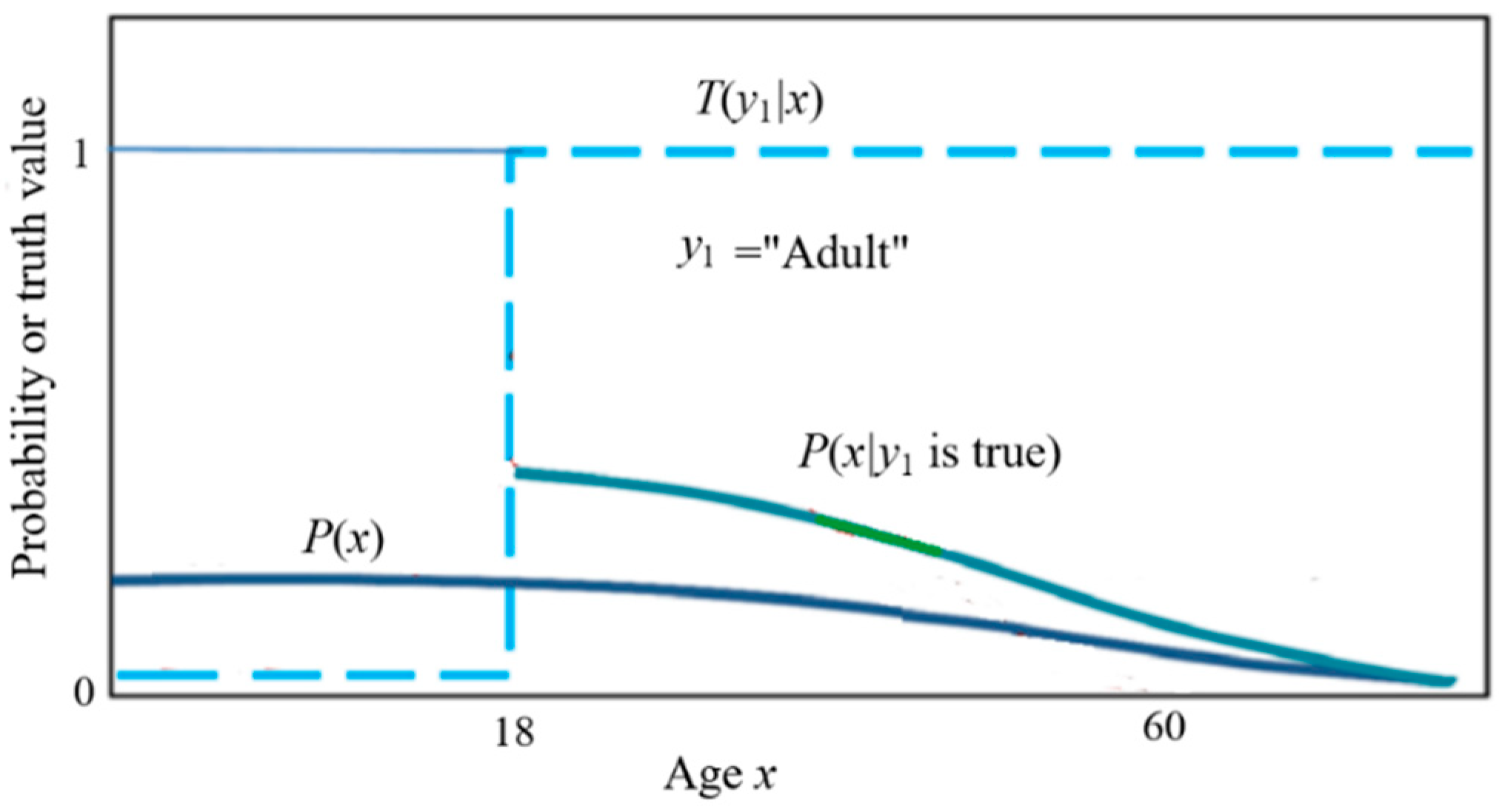
Figure 2.
A GPS device's positioning with a deviation. The round point is the pointed position with a deviation, and the place with the star is the most possible.
Figure 2.
A GPS device's positioning with a deviation. The round point is the pointed position with a deviation, and the place with the star is the most possible.
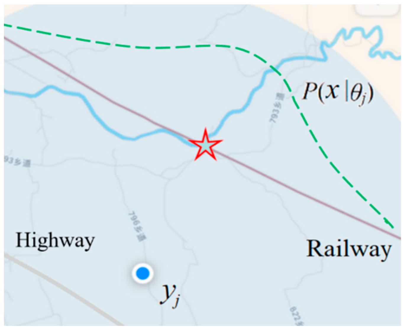
Figure 3.
The Shannon channel (a) and the semantic channel (b).
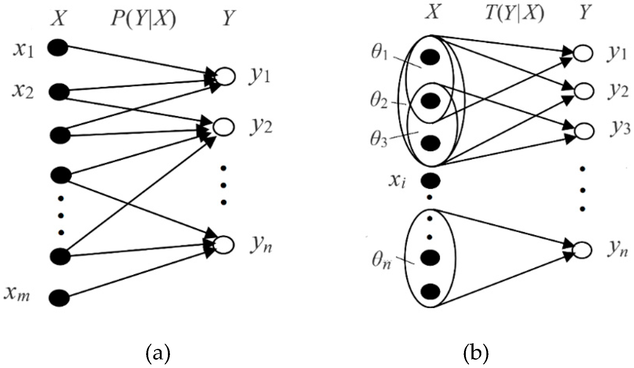
Figure 4.
Communication models. (a) The Shannon communication model where the channel needs to match the distortion function. (b) The semantic communication models where two channels need to match mutually.
Figure 4.
Communication models. (a) The Shannon communication model where the channel needs to match the distortion function. (b) The semantic communication models where two channels need to match mutually.
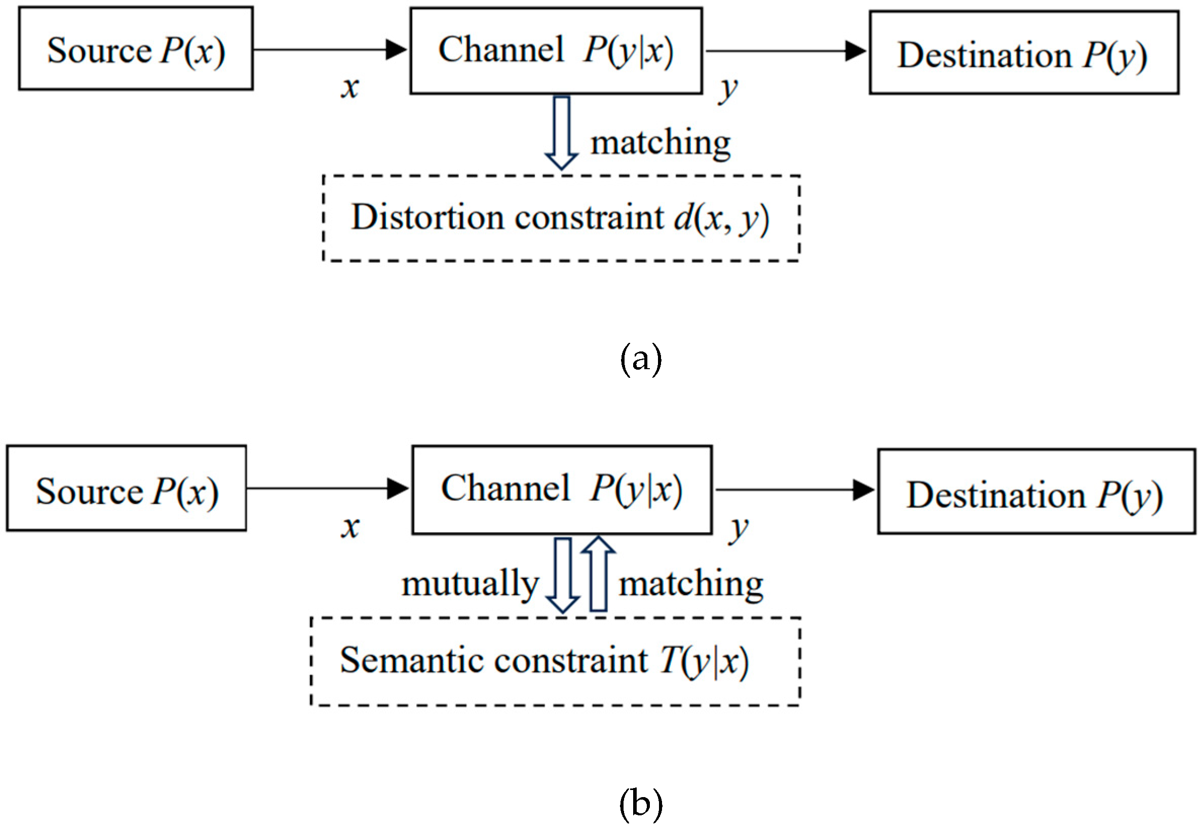
Figure 5.
Semantic information yj conveys about xi decreases with the deviation or distortion increasing.
Figure 5.
Semantic information yj conveys about xi decreases with the deviation or distortion increasing.
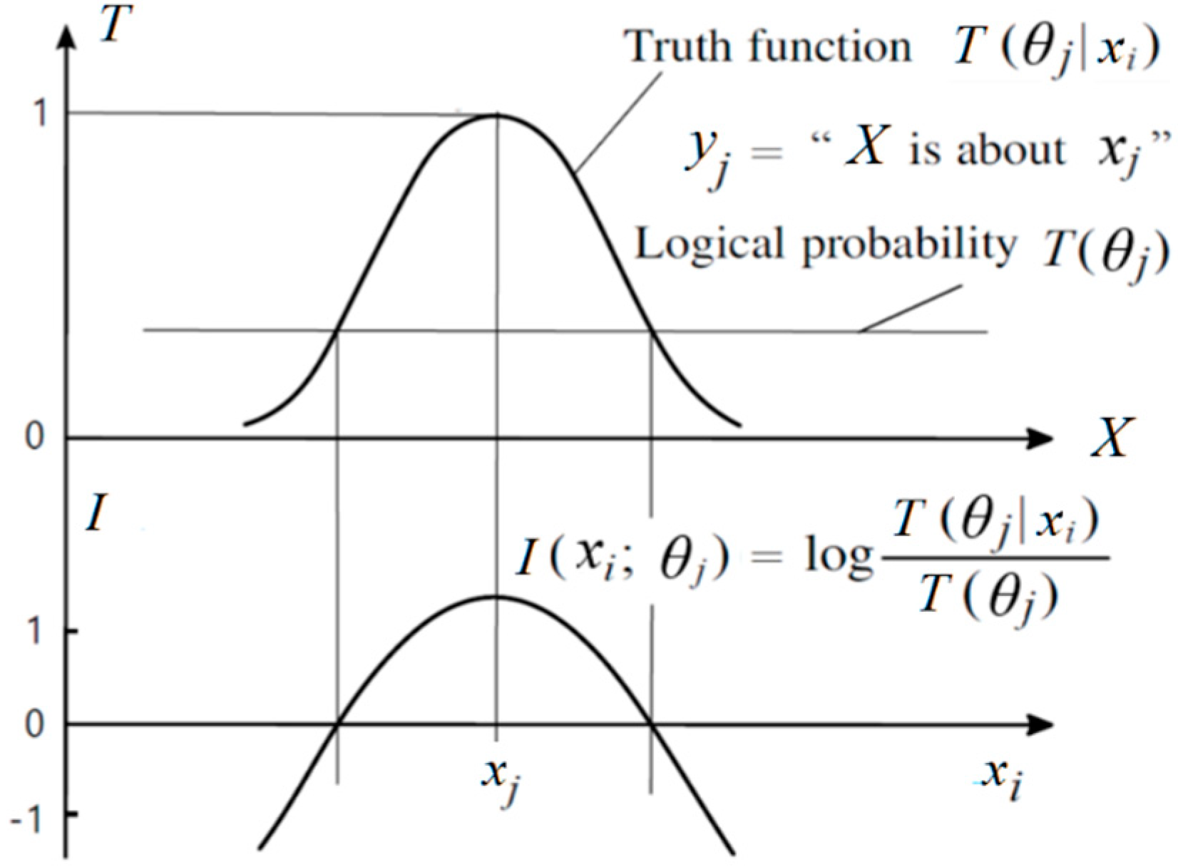
Figure 6.
The information rate-fidelity function R(G) for binary communication. Any R(G) function is a bowl-like function. There is a point at which R(G) = G (s = 1). For given R, two anti-functions exist: G-(R) and G+(R).
Figure 6.
The information rate-fidelity function R(G) for binary communication. Any R(G) function is a bowl-like function. There is a point at which R(G) = G (s = 1). For given R, two anti-functions exist: G-(R) and G+(R).
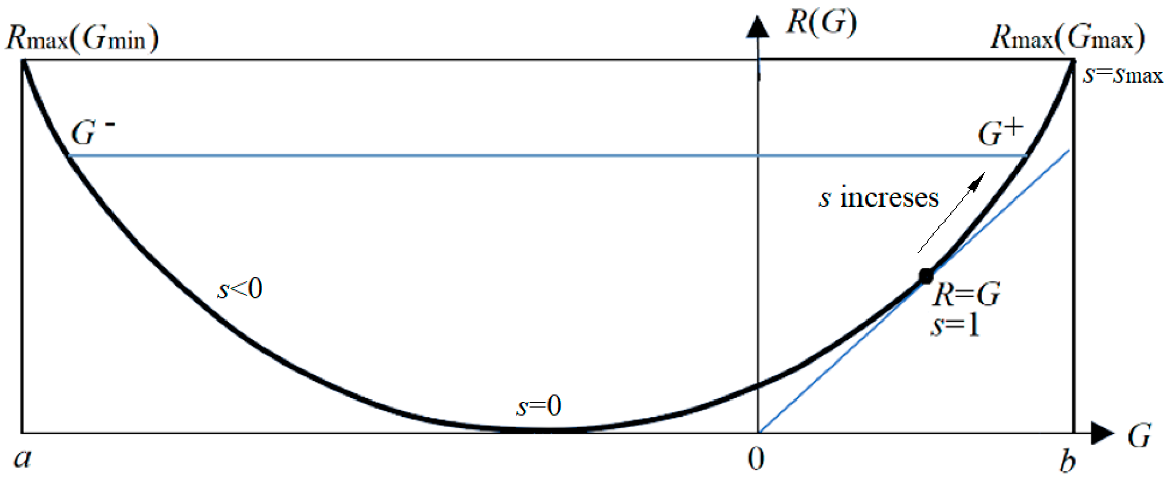
Figure 7.
The electronic semantic communication model. The distortion constraint is replaced with the semantic information loss constraint.
Figure 7.
The electronic semantic communication model. The distortion constraint is replaced with the semantic information loss constraint.
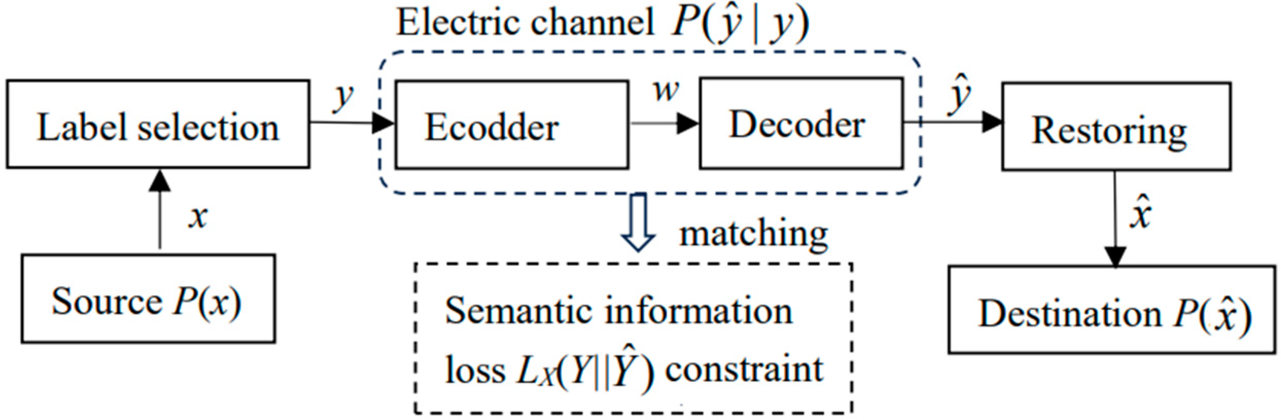
Figure 8.
The iteration results of Example 2. (a) 8 truth value functions or the semantic channels T(y|x) (see Appendix C in [28] for the Data generation method). (b) Convergent Shannon channel P(y|x). (c) The variation of I(X; Yθ) and I(X; Y) during iteration.
Figure 8.
The iteration results of Example 2. (a) 8 truth value functions or the semantic channels T(y|x) (see Appendix C in [28] for the Data generation method). (b) Convergent Shannon channel P(y|x). (c) The variation of I(X; Yθ) and I(X; Y) during iteration.

Figure 9.
Variation of R(G) function with discrimination (σ=1/64 or σ=3/64) for a given quantization level b=63.
Figure 9.
Variation of R(G) function with discrimination (σ=1/64 or σ=3/64) for a given quantization level b=63.
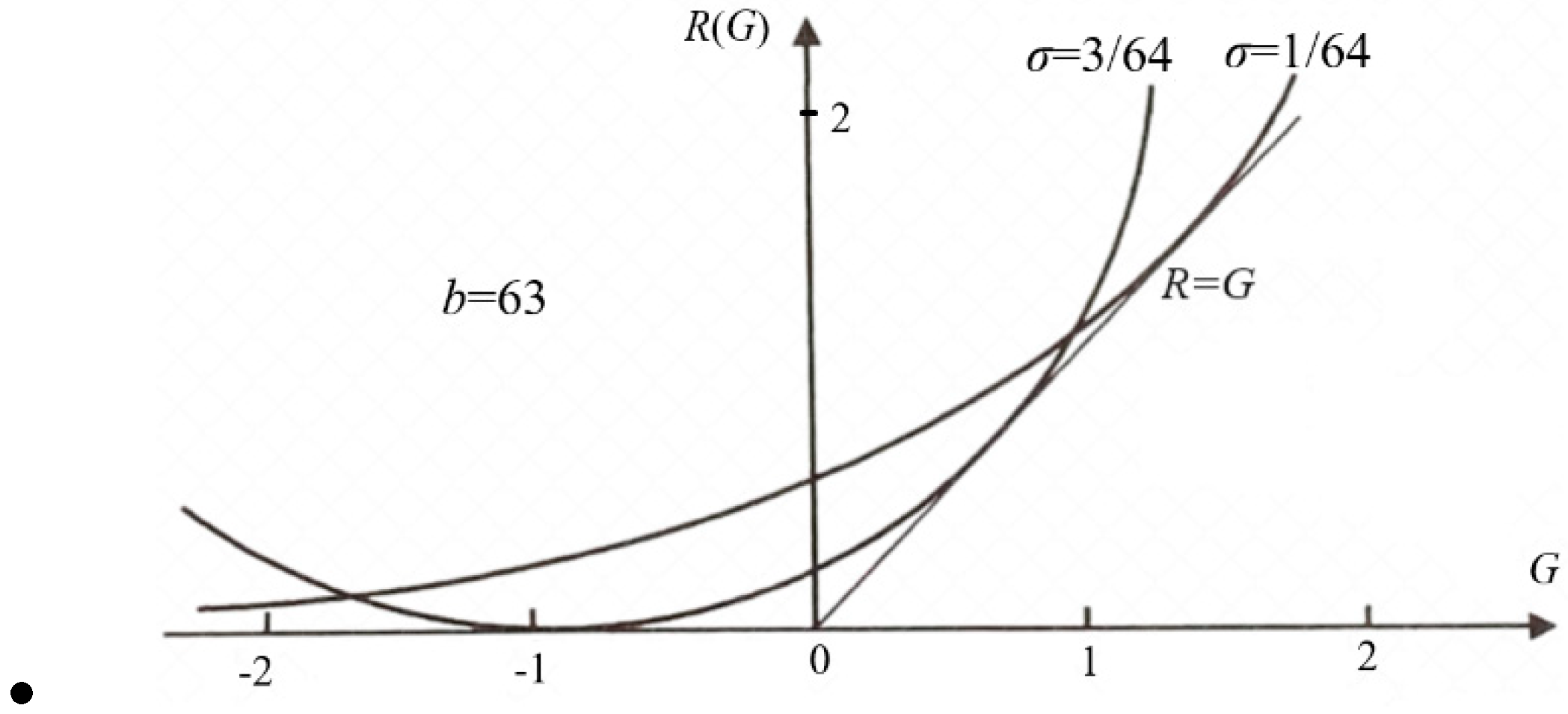
Figure 10.
The optimization methods of the two types of semantic information are different. For predictive information, we hope that P(x|θj) is close to P(x|yj) (see white arrow); while for Goal-oriented information, we hope that P(x|aj) is close to P(x|θj) (see black arrow).
Figure 10.
The optimization methods of the two types of semantic information are different. For predictive information, we hope that P(x|θj) is close to P(x|yj) (see white arrow); while for Goal-oriented information, we hope that P(x|aj) is close to P(x|θj) (see black arrow).
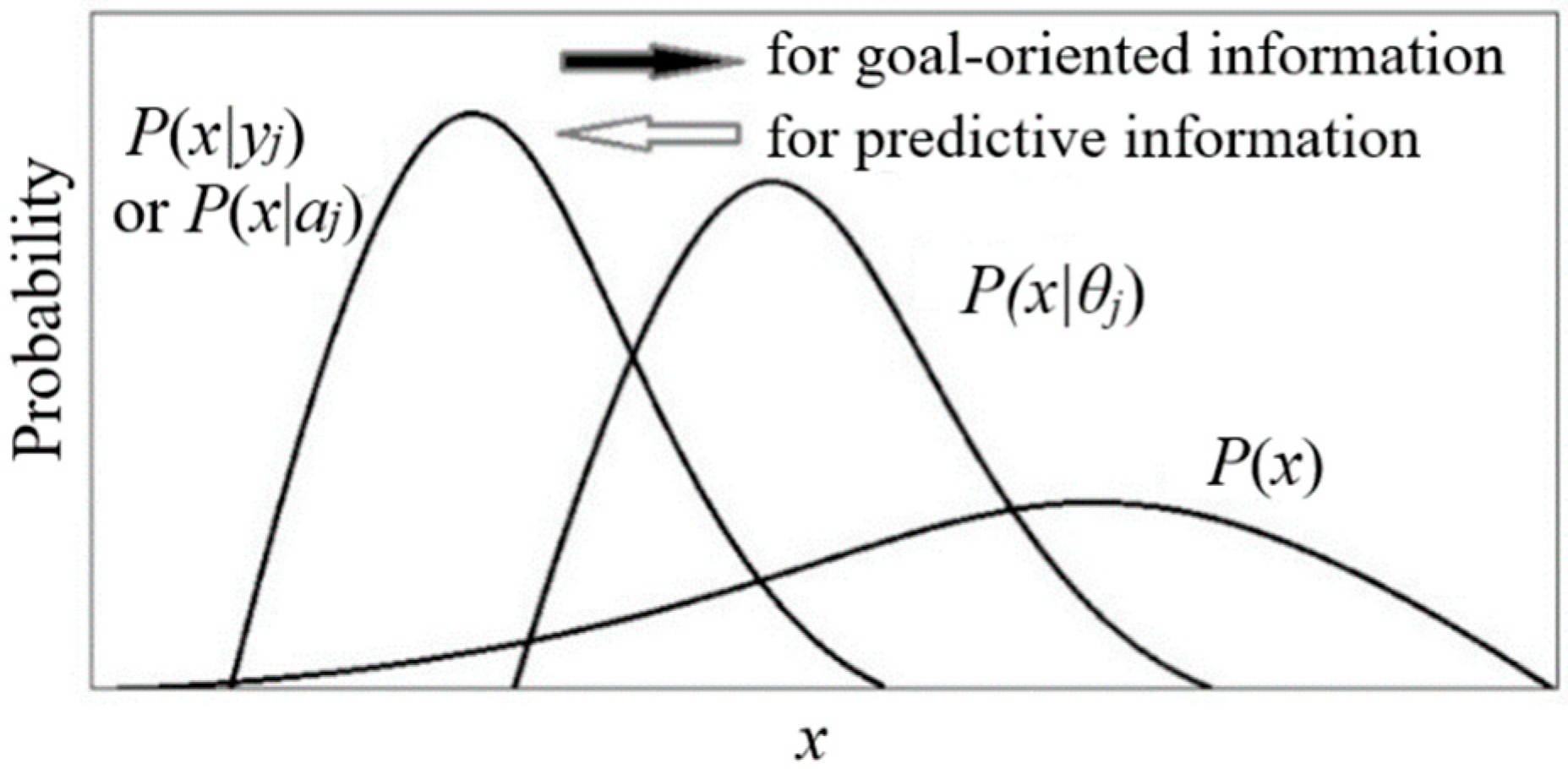
Figure 11.
A two-objective control task. Dashed lines show P(x|aj)=P(x|θj, s) (j=0, 1), and dash-dotted lines representing P(x|βj, s) (j=0,1). (a) For the case with s=1; (b) For the case with s=5. P(x|βj, s) is a normal distribution produced by action aj.
Figure 11.
A two-objective control task. Dashed lines show P(x|aj)=P(x|θj, s) (j=0, 1), and dash-dotted lines representing P(x|βj, s) (j=0,1). (a) For the case with s=1; (b) For the case with s=5. P(x|βj, s) is a normal distribution produced by action aj.
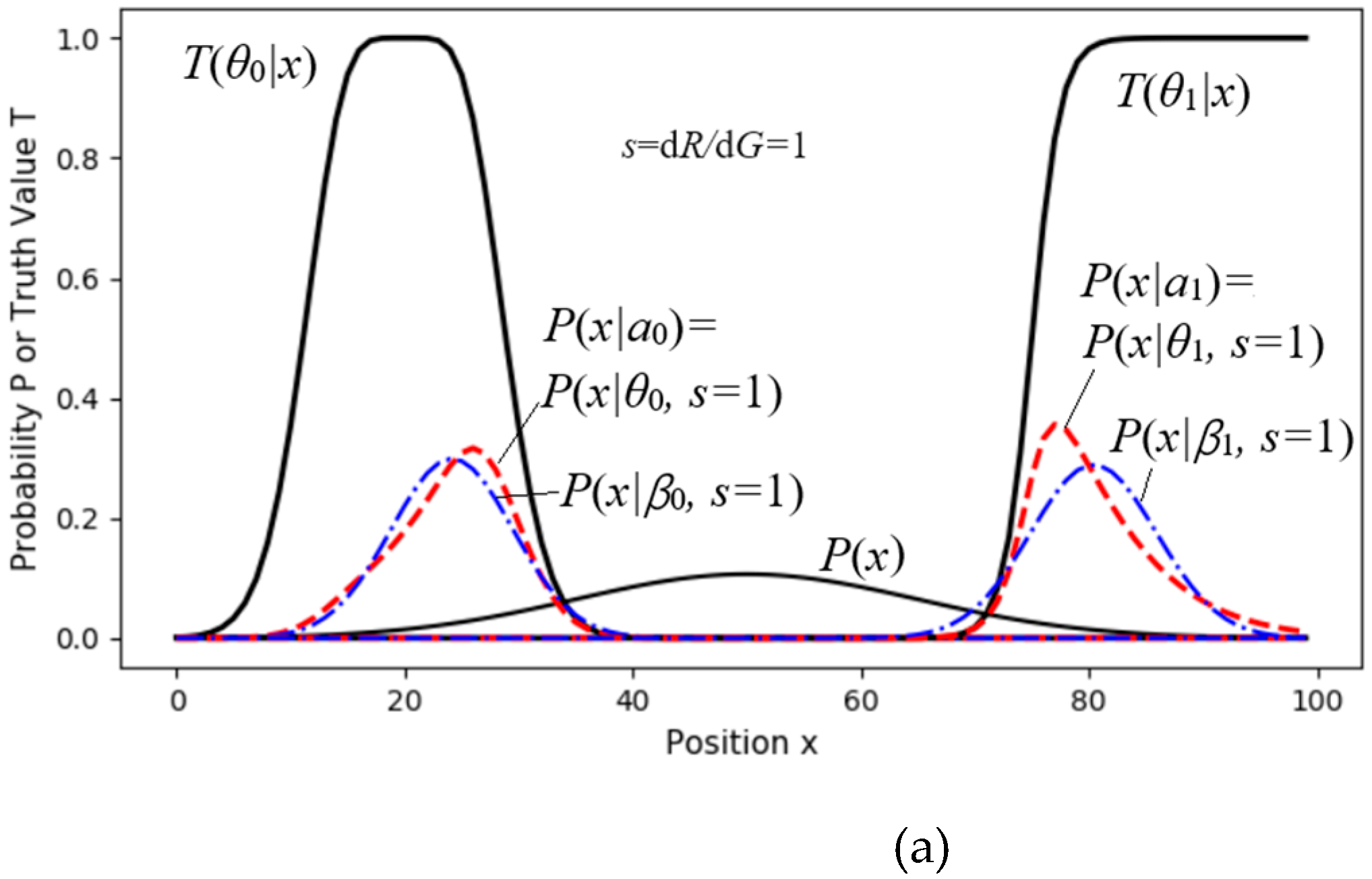
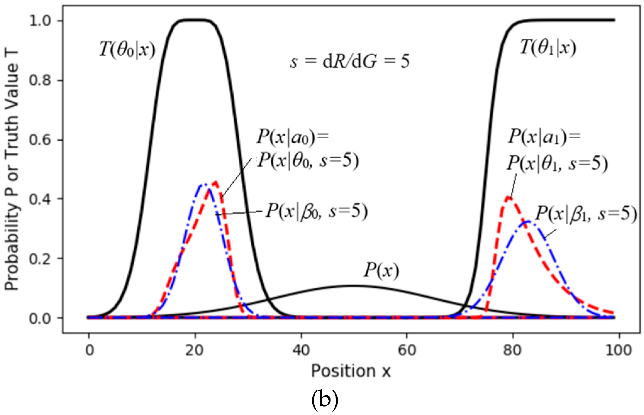
Figure 12.
The R(G) for constraint control. G slightly increases when s increases from 5 to 40, meaning s=5 is good enough.
Figure 12.
The R(G) for constraint control. G slightly increases when s increases from 5 to 40, meaning s=5 is good enough.
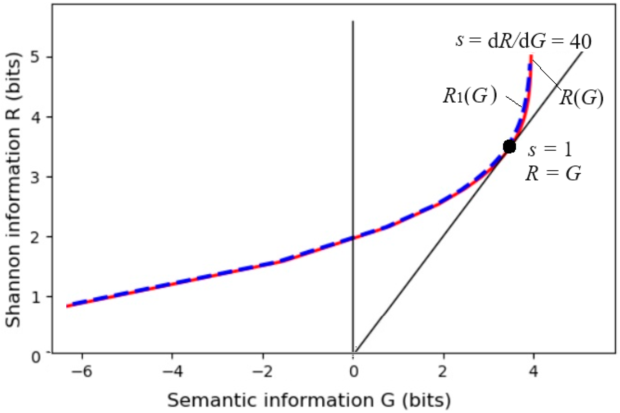
Disclaimer/Publisher’s Note: The statements, opinions and data contained in all publications are solely those of the individual author(s) and contributor(s) and not of MDPI and/or the editor(s). MDPI and/or the editor(s) disclaim responsibility for any injury to people or property resulting from any ideas, methods, instructions or products referred to in the content. |
© 2025 by the authors. Licensee MDPI, Basel, Switzerland. This article is an open access article distributed under the terms and conditions of the Creative Commons Attribution (CC BY) license (http://creativecommons.org/licenses/by/4.0/).
Copyright: This open access article is published under a Creative Commons CC BY 4.0 license, which permit the free download, distribution, and reuse, provided that the author and preprint are cited in any reuse.


