
Submitted:
29 April 2025
Posted:
30 April 2025
You are already at the latest version
Abstract
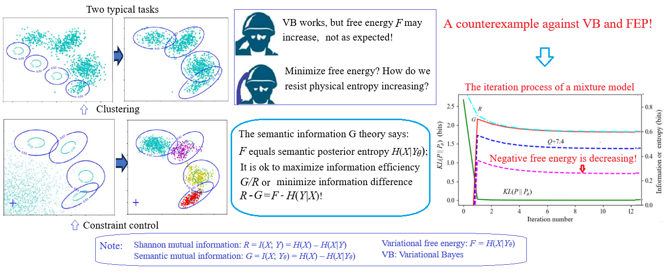
Friston proposed the Minimum Free Energy (MFE) principle based on the Variational Bayesian (VB) method. This principle inherits the basic idea of Evolutionary System Theory. Still, it emphasizes the coordination between the brain, behavior, and the environment, promoting self-organization. However, there are two issues with VB and the MFE principle: 1) When using VB to optimize latent variables, the Variational Free Energy (VFE) F may not always decrease; 2) The concept of VFE is inconsistent with physical free energy. The author proposed the semantic information G theory and R(G) function 30 years ago (R is the minimum mutual information for the given semantic mutual information G). Based on the study of the R(G) function, this paper proposes the Semantic Variational Bayesian (SVB) and the Maximum Information Efficiency (MIE) principle to resolve the two issues with VB and the MFE principle. Theoretic analysis and computing experiments prove that R–G = F-H(X|Y) instead of F continues to decrease when optimizing latent variables. The experiments show that SVB is reliable and straightforward for latent variables and active inference. This paper also explains the relationship between information, entropy, and free energy in local non-equilibrium and equilibrium systems, concluding that Shannon's information is similar to free energy's increment, semantic information is similar to exergy's increment, and VFE is equivalent to some physical entropy. The MIE principle inherits the basic idea of the MFE principle but is easier to understand and apply.
Keywords:
variational Bayes
; free energy principle
; entropy
; Shannon mutual information
; semantic mutual information
; information rate-distortion
; EM algorithm
; active inference
; free energy
; Boltzmann distribution
1. Introduction
In 1993, Hinton et al. [1,2] used the minimum free energy as an optimization criterion to improve neural network learning, which led to significant breakthroughs. This method was later developed into the Variational Bayesian (VB) approach [3,4], which has since been widely and successfully applied in machine learning (including reinforcement learning) [5]. Friston [6,7] extended the application of VB to neuroscience, evolving the Minimum Free Energy (MFE) criterion into the MFE principle, aiming for it to become a unified scientific theory of brain function and biological behavior. This theory integrates concepts such as predictive coding, perceptual prediction, active inference, information, and stochastic dynamical systems [7–9]. Unlike the passive perspective in the book Entropy: A New World View [10], Friston’s theory inherits the optimistic entropy-based worldview from the existing Evolutionary Systems Theory (EST) [11,12] and emphasizes the ability of bio-organisms to predict, adapt to, and influence their environment, which promotes self-organization and order.
Friston’s theory has garnered widespread attention and deep reflection [13]. Many applications have emerged [14]. Information and free energy have been combined to explain self-organization and order [15,16]. However, some criticisms have also been raised. Some argue that free energy means negative entropy and is essential for life; thus, minimizing free energy would imply death [17]. Others contend that while the MFE principle is valuable as a tool, its validity as a universal principle or falsifiable scientific law remains debatable.
As early as 1990, Silverstein and Pimbley [18] used “minimum free energy method” in the title of their article. Their objective function is defined as a linear combination of the mean-square error energy expression and the signal entropy expression. In the paper entitled Two Kinds of Free Energy and the Bayesian Revolution, Gottwald and Braun [19] reviewed many similar studies and argued that Friston’s free energy is just one of the two kinds. The other kind uses various objective functions in Maximum Entropy (ME) methods. These objective functions either equal the reward function plus the entropy function (which needs to be maximized) or the average loss minus the entropy function (which needs to be minimized). Both kinds of free energy methods are very significant. But in my opinion, Friston’s MFE principle is different from the ME principle [20,21] for the following reasons:
- Subjective prediction and objective reality (or objective reality and subjective goals) approach each other bidirectionally and dynamically.
- Loss functions are expressed in terms of information or entropy measures, transforming the active inference issue into the inverse issue of sample learning.
- Multi-task coordination and tradeoffs exist, requiring solving latent variables.
It seems that the MFE principle can better explain the subjective initiative of bio-organisms than the ME principle. However, from the author’s perspective, the MFE principle is still imperfect because it has two issues. Below, we refer to free energy in VB and the MFE principle as Variational Free Energy (VFE).
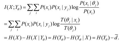
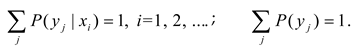
Thirty years ago, the author extended Shannon’s information theory to a semantic information theory [22–24]. The formula for semantic Mutual Information (MI) is: I(X; Yθ)=H(X)–H(X|Yθ), where H(X|Yθ) is the semantic posterior entropy or posterior cross-entropy. Roughly speaking, H(X|Yθ) equals VFE; minimizing VFE is equivalent to maximizing semantic MI. Later, the author called the generalized theory the Semantic Information G Theory [25,26] (or simply the G Theory, where “G” stands for “generalization”) for machine learning. The author recognized early that H(X|Yθ) does not necessarily decrease monotonically when a Shannon channel matches a semantic channel. The author also studied mixture models with the Expectation-Maximization (EM) algorithm [25]. Experimental observations indicated that H(X|Yθ) and VFE do not continually decrease as the mixture model converges. Although VB ensures the mixture model’s convergence [2,3], its theoretical justification is flawed. This is the first issue with VB and the MFE principle.
The second issue concerns the relationship between VFE and physical entropy and free energy. There is an apparent contradiction. In physics, free energy is the energy available to perform work and is usually maximized [27]. If we actively minimize free energy, aren’t we simply following the trend of increasing entropy [17]? Thus, we must clarify what VFE or H(X|Yθ) truly represents in thermodynamic systems and how information, entropy, and free energy mutually relate in such systems.
As early as 1993, the author [23] analyzed information between temperature and a molecule’s energy in a local no-equilibrium and equilibrium system. The conclusions include that Shannon MI is similar to the increment of free energy in a local no-equilibrium system; semantic MI is similar to the increment of free energy in a local equilibrium system. In addition, the author extended Shannon’s rate-distortion function R(D) to obtain the information rate-fidelity function R(G) [23,25], where R represents the minimum Shannon MI for given semantic MI G (representing fidelity). The method for solving R(G) can be called the Semantic Variational Bayesian (SVB) method [28]. SVB can solve issues VB addresses but does not always minimize VFE. Instead, it minimizes R−G=F−H(X∣Y). Minimizing R−G is equivalent to maximizing information efficiency: G/R. Thus, the author proposes the Maximum Information Efficiency (MIE) principle. This principle can overcome the two issues with VB and the MFE principle. The applications of the G Theory in machine learning include multi-label learning, maximum MI classification for unseen instances, mixture models [25], Bayesian confirmation [26], and semantic compression [29]. The success of these applications strengthens the validity of the G Theory.
The motivation of this paper is to clarify the above two issues existing in VB and the MFE principle and to improve them. This paper aims to provide an improved version of the MFE principle.
The contributions of this paper:
- Mathematically clarifying the theoretical and practical inconsistencies in VB and the MFE principle.
- Explaining the relationships between Shannon MI, semantic MI, VFE, and physical entropy with free energy from the perspectives of the G Theory and statistical physics.
- Providing experimental evidence by mixture model examples (including one used by Neal and Hinton [2]) to demonstrate that VFE may increase during the convergence of mixture models and explain why this occurs.
The iteration method for minimum information difference in SVB is inspired by the iterative approach used by Shannon et al. in solving the rate-distortion function [30–32].
Abbreviations and explanations can be found in Appendix A. Information about Python source codes for producing most figures in this paper can be found in Appendix B.
2. Two Typical Tasks of Machine Learning
2.1. Sheep Clustering: Mixture Models
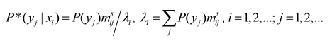
To explain the tasks to be completed by VB. Let’s take sheep clustering and sheep herding as examples. This section describes the sheep clustering issue (see Figure 1).
Suppose several sheep flocks are distributed on a grassland with fuzzy boundaries. We can observe that the density distribution (the proportion of the number of sheep per unit area) is P(x). We also know there are n flocks of sheep, and the distributions have a certain regularity, such as the Gaussian distribution. We can establish a mixture model: Pθ(x) = P(y1)P(x|θ1) + P(y2)P(x|θ2) +… Then, we use the maximum likelihood criterion or the minimum cross entropy criterion to optimize the mixture ratios P(y1), P(y2), … and model parameters.
The Expectation-Maximization (EM) algorithm [33,34] is usually used to solve the mixture model. This algorithm is very clever. It can automatically adjust the different components, namely the likelihood function (circled in Figure 1), so that each component covers a group of instances (a flock) and can provide the appropriate ratios P(yj), j=1,2,3,4, of the mixture model’s components, also known as the probability distribution of the latent variable. We sometimes call P(y) the latent variable.
The EM algorithm is not ideal in two aspects: 1) There have been problems with its convergence proof [25], which has led to blind improvements; 2) P(y) sometimes converges very slowly, and it is challenging to solve P(y) when the likelihood functions remains unchanged. Researchers use VB not only to improve the EM algorithm [2,3] but also to solve latent variables [5].
The mixture model belongs to unsupervised learning in machine learning and is very representative. Similar methods can be found in Restricted Boltzmann Machines and deep learning pre-training tasks.
2.2. Driving the Sheep to Pastures: Constrained Control and Active Inference
Driving sheep to pastures is the constraint control issue of random events and also the active inference issue involving reinforcement learning. In this case, Shannon’s MI reflects the control complexity. We need to maximize the purposefulness (or utility) and minimize the Shannon MI, the control cost.
The circles in the figure represent the control targets; the points in Figure 2a reflect the initial flock density distribution P(x). There are usually two types of control objectives or constraints:
- The objectives are expressed by the probability distributions P(x|θj)(j=1,2,3,4). Given P(x) and P(x|θj), we solve the Shannon channel P(y|x) and the herd ratio P(y). It is required that P(x|yj) is close to P(x|θj) and P(y) can minimize the control cost.
- The objectives are expressed by the fuzzy ranges. P(x|θj) (j=1,2, …) can be obtained from P(x) and the fuzzy ranges, and the others are the same.
Circles in Figure 2 represent constraint ranges. The difference between clustering in mind (see Figure 1) and herding in reality (see Figure 2): for clustering, P(x) is fixed, and the herd ratios are objective; for herding, P(x) is transferred to the target areas, and the herd ratios are adjusted according to the minimum control cost criterion. For example, when clustering, the proportions of the two groups of sheep in the middle are larger; when herding, the proportions of the two groups on the sides are larger because it is easier to drive sheep there. In addition, the centers of four groups of sheep in Figure 2b deviate from the target centers, which is also for the sake of control cost. We can also increase the constraint strength to drive the sheep to the ideal position. However, the control cost must also be considered. Both sheep clustering and herding require solving latent variables.
3. The Semantic Information G Theory and the Maximum Information Efficiency Principle
3.1. The P-T Probability Framework
Why do we need the P-T probability framework? The reasons are:
- The P-T probability framework [26] allows us to use truth, membership, similarity, and distortion functions as constraints in addition to the likelihood function to solve the latent variables.
- A hypothesis or label, such as “adult”, has two probabilities: statistical probability, defined by Mises [35], and logical probability, defined by Kolmogorov [36]. The former is normalized, whereas the latter is not.
The P-T probability framework is denoted by a five-tuple (U, V, B, P, T), where
- U={x1, x2, …} is a set of instances, X∈U is a random variable;
- V={y1, y2, …} is a set of labels or hypotheses, Y∈V is a random variable;
- B={θ1,θ2, …} is the set of subsets of U; every subset θj has a label yj∈V.
- P is the probability of an element in U or V, i.e., the statistical probability; it is defined with “=”, such as P(xi)=P(X=xi).
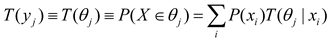
- T is the probability of a subset of V or an element in B, i.e., the logical probability; it is defined with “∈”, such as T(yj)=P(X∈θj).
In addition, we assume θjis a fuzzy set and also a model parameter.
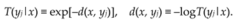
The truth value of yj for given x is the membership grade of x in θj, which is also the conditional logic probability of yj, namely:
T(yj|x) ≡ T(θj|x) ≡ mθj (x).
According to Davidson’s truth-conditional semantics [39], T(yj|x) reflects the semantics of yj. The logical and statistical probabilities of a label are often not equal. For example, the logical probability of a tautology is 1, while its statistical probability is close to 0. We have P(y1) + P(y2) + … + P(yn) = 1, but it is possible that T(y1) + T(y2) + … + T(yn) > 1.
According to the above definition, we have:
As we will see later, T(yj) is the statistical physics’ partition function and machine learning’s regularization term. We can put T(θj|x) and P(x) into Bayes’ formula to obtain the semantic probability prediction formula [25]:
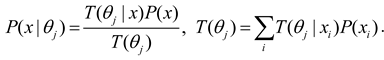
P(x|θj) is the likelihood function P(x|yj, θ) in the popular method. We call the above formula the semantic Bayes’ formula.
Just as a set of transition probability functions P(yj|x)( j=1, 2, …) constitutes a Shannon channel, a set of truth functions T(θj|x) (j=1,2,…) constitutes a semantic channel.
The relationship between the truth function and the distortion function is [29]:
3.2. The Semantic Information Measure and Information Rate-Fidelity Function
Shannon MI can be expressed as.
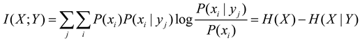
We replace P(xi|yj) on the right side of the log with the likelihood function P(xi|θj), leaving the left P(x|yj) unchanged. Hence, we get the semantic MI:
The Explanation of the last line can be found in Appendix C, which also includes the Logical Bayes’ Inference [25] for solving T(θj|x) from P(yj|x) or P(x|yj) and P(x).
Roughly speaking, semantic posterior entropy H(X|Yθ) is VFE F in VB and the MFE principle. The smaller it is, the greater the amount of semantic information.
Semantic MI is less than or equal to the Shannon MI and reflects the average code length saved due to the semantic prediction. It is easy to see that the maximum semantic MI criterion is equivalent to the maximum likelihood criterion and is similar to the Regularized Least Squares (RLS) criterion. Semantic entropy Hθ(Y) is the regularization term. Fuzzy entropy H(Yθ|X) is a more general average distortion than the average square error.
Suppose the truth function becomes a similarity function. In that case, the semantic MI becomes the estimated MI [25]. For example, when calculating the information of the GPS pointer or the color perception, the truth function becomes the similarity function, which can be represented by a Gaussian function [25]. The estimated MI has been used by deep learning researchers for Mutual Information Neural Estimation (MINE) [39] and Information Noise Contrast Estimation (InfoNCE) [40].
Shannon [30] defines that given a source P(x), a distortion function d(y|x), and the upper limit D of the average distortion , we change the channel P(y|x) to find the minimum MI, R(D). R(D) is the information rate-distortion function.
Now, we replace d(yj|xi) with I(xi; θj)=log[T(θj|xi)/T(θj), replace with I(X; Yθ), and replace D with the lower limit G of the semantic MI to find the minimum Shannon MI, R(G). R(G) is the information rate-fidelity function. Because G reflects the average code length saved due to semantic prediction, using G as the constraint is more consistent in shortening the code length, and G/R can better represent information efficiency.
The R(G) function is defined as
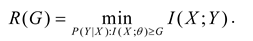
We use the Lagrange multiplier method to find the minimum MI. The constraint conditions include I(X; Yθ)≥G and
The Lagrangian function is:

Using P(y|x) as a variation, we let . Then, we obtain:
 where mij=P(xi|θj)/P(xi)=T(θj|xi)/T(θj). Using P(y) as a variation, we let . Then, we obtain:
where P*(yj) means the next P(yj). Because P*(y|x) and P*(y) are interdependent, we can first assume a P(y) and then repeat the above two formulas to obtain convergent P*(y) and P*(y|x) (see [36] (P. 326)). We call this method the Minimum Information Difference (MID) iteration. Someone may ask: Why do we obtain Equation (11) through variational methods instead of directly using Equation (11)? If we use Equation (11) directly, we still need to prove that P*(y) reduces R–G.
where mij=P(xi|θj)/P(xi)=T(θj|xi)/T(θj). Using P(y) as a variation, we let . Then, we obtain:
where P*(yj) means the next P(yj). Because P*(y|x) and P*(y) are interdependent, we can first assume a P(y) and then repeat the above two formulas to obtain convergent P*(y) and P*(y|x) (see [36] (P. 326)). We call this method the Minimum Information Difference (MID) iteration. Someone may ask: Why do we obtain Equation (11) through variational methods instead of directly using Equation (11)? If we use Equation (11) directly, we still need to prove that P*(y) reduces R–G.
Any R(G) function is bowl-shaped (possibly not symmetrical) [24], with the second derivative greater than 0. The s = dR/dG is positive on the right. When s = 1, G equals R, meaning the semantic channel matches the Shannon channel. G/R represents information efficiency; its maximum is 1. G has a maximum value, G+, and a minimum value, G–, for given R. G– means how small the semantic information the receiver receives can be when the sender intentionally lies.
3.3. Semantic Variational Bayes and the Maximum Information Efficiency Principle
Using P(x|θj) as the variation and letting , we get P(x|θj)=P(x|yj) or T(θj|x) ∝ P(yj|x), which is the result of LBI. Therefore, the MID iteration plus LBI plus equals SVB. When using SVB to solve the latent variables, the constraint functions can be likelihood functions, truth (or membership) functions, similarity functions, and distortion functions (or loss functions). When the constraint is a set of likelihood functions, the MID iteration formulas are:
When the constraint is a set of truth or similarity functions, the formulas become:
The hyperparameter s allows us to strengthen the constraint to reduce the ambiguity of boundaries. Therefore, the Shannon channel can also be regarded as a fuzzy classification function. Ambiguity reduces semantic MI but saves Shannon MI.
Under the premise that G is large enough, using the MID criterion means using the MIE criterion. Applying this criterion to various fields is to use the MIE principle. Note that the MIE principle does not only maximize G/R; it maximizes G/R under the condition that G meets the requirement. This requires us to balance between maximizing G and maximizing G/R. As a constraint condition, G is not only about limiting the amount of semantic information but also about specifying what kind of semantic information is needed. It is related to human purposes and needs. Therefore, the MIE principle is associated with information values.
4. The Maximum Information Efficiency Principle for Mixture Models and Constrained Control
4.1. New Explanation of the EM Algorithm for Mixture Models (About Sheep Clustering)
The EM algorithm [41,42] is usually used for the mixture model, an unsupervised learning (clustering) method. We know that P(x) = ∑ j P(yj) P(x|yj). Given a sample distribution P(x), we use Pθ(x) = ∑ j P(x|θj)P(yj) to approximate P(x) so that the relative entropy or KL divergence KL(P‖Pθ) is close to 0.
The EM algorithm first presets P(x|θj) and P(yj). The E-step obtains:
In the M-step, the log-likelihood of the complete data (usually represented by Q) is maximized. The M-step can be divided into two steps: the M1-step for
and the M2-step for
For Gaussian mixture models, we can use the expectation and standard deviation of P(x)P(yj|x)/P+1(yj) as those of P(x|θj+1). P+1(y) is the above P*(y).
From the perspective of the G theory, the M2-step is to make the semantic channel match the Shannon channel, the E-step is to make the Shannon channel match the semantic channel, and the M1-step is to make the destination P(y) match the source P(x). Repeating the above three steps can make the mixture model converge.
However, there are two problems with the EM algorithm: 1) P(y) may converge slowly; 2) If the likelihood functions are also fixed, how do we solve P(y)?
Based on the R(G) function analysis, the authors improved the EM algorithm to the EnM algorithm [25,31]. The E-step in the EnM algorithm remains unchanged, and the M-step is the M2-step in the EM algorithm. In addition, The n-step is added after the E-step. It repeats Equations (15) and (16) to calculate P(y) n times so that P+1(y) ≈ P(y). The EnM algorithm also uses the MIE criterion. The n-step can speed up P(y) matching P(x). The M-step only optimizes likelihood functions. Because after n-step, P(yj)/P+1(yj) is close to 1, we can use the following formula to optimize the model parameters:
Without the n-step, there will be P(yj) ≠ P+1(yj), and ∑ i P(xi)P(x|θj)/Pθ(xi) ≠ 1.
When solving the mixture model, we can choose a smaller n, such as n=3. When solving P(y) specifically, we can select a larger n until P(y) converges. When n=1, the EnM algorithm becomes the EM algorithm.
We can deduce that after the E-step, there is (see Appendix D for the proof):
where KL(P||Pθ) is the relative entropy or KL divergence between P(x) and Pθ(x); KL(PY+1||PY) is KL(P+1(y))||P(y)), which is close to 0 after the M1 step or the n-step.
Equation (19) can be used to prove the convergence of mixture models because the M2-step maximizes G, and the E-step and n-step minimize R–G and KL(PY+1||PY), H(P‖Pθ) can be close to 0. The MIE principle is used. Experiments have shown that as long as the sample was large enough, Gaussian mixture models of n=2 would converge globally.
If the likelihood functions are fixed, the EnM algorithm becomes the En algorithm. The En algorithm can be used to find the latent variable P(y) for fixed constraint functions.
4.2. Goal-Oriented Information and Active Inference (About Sheep Herding)
In the above, we use the G measure to measure semantic information in communication systems, requiring that the prediction P(x|θj) conforms to the fact P(x|yj). Goal-oriented information is the opposite, requiring the fact to conform to the goal. We also call this information control information or purposeful information [28].
An imperative sentence can be regarded as a control instruction. We need to know whether the control result conforms to the control goal. The more consistent the result is, the more information there is. A likelihood function or a truth function can represent a control goal. The following goals can be expressed as truth functions:
- “The grain production should be close to or exceeds 7500 kg/hectare”;
- “The age of death of the population should preferably exceed 80 years old”;
- “The cruising range of electric vehicles should preferably exceed 500 kilometers”;
- “The error of train arrival time should preferably not exceed 1 minute”.
Semantic KL information can be used to measure purposeful information:
In this formula, θj indicates that the control target is a fuzzy range, and aj is an action selected for task yj. In the above formula, yj is replaced with aj. One reason is that we may select different aj for the same task yj; another reason is that aj is used in the popular active inference method for the same purpose.
If there are several control targets y1, y2, … we can use the semantic MI formula to express the purposeful information:
where A is a random variable taking a value aj. Using SVB, the control ratio P(a) can be optimized to minimize the control complexity (i.e., Shannon MI) for given I(X; A/θ).
Goal-oriented information can be regarded as the cumulative reward function in reinforcement learning. However, the goal here is a fuzzy range representing a plan, command, or imperative sentence. The optimization task is similar to the active inference task using the MFE principle. For a multi-target task, the objective function to be minimized is:
f = I(X; A) – sI(X;A/θ).
When the actual distribution P(x|aj) is close to P(x|θj), the information efficiency reaches its maximum value,1. To further increase both information, we can use the MID iteration with s to get P(aj|x) and P(a) and use Bayes’ formula to obtain
We may use the likelihood function P(x|θj) or the truth function T(θj|x) for the sheep-herding task to represent goals, respectively. We may change Equation (23) for different constraint functions, referring to Equations (13) and (14). Compared with VB, the above method is simpler and can change the constraint strength by s.
For both communication and constraint control (or active inference), G stands for the effect, R for the cost, and G/R for the efficiency. We collectively refer to G/R in both cases as information efficiency.
5. The Relationship Between Information and Physical Entropy and Free Energy
5.1. Entropy, Information, and Semantic Information in Local Non-equilibrium and Equilibrium Thermodynamic Systems
Gibbs set up the relationship between thermodynamic entropy and Shannon’s entropy; Jaynes [20,21] proved that according to Stirling’s formula, lnN! = NlnN − N (when N→∞), there is a simple connection between Boltzmann’s microscopic state number Ω of N molecules and Shannon entropy:
where S is entropy, k is the Boltzmann constant, xi is the i-th microscopic state (i =1,2,…, Gm; Gm is the microscopic state number of one molecule), N is the number of molecules that are mutually independent, Ni is the number of molecules with xi, and T0 is the absolute temperature. P(xi|T0) = Ni/N represents the probability of a molecule in a state xi at temperature T0. The Boltzmann distribution for a given energy constraint is:
where Z’ is the partition function.
Information and entropy in Thermodynamic Systems have been discussed by researchers [15,41], but the following methods and conclusions are different.
Considering the information between temperature and molecular energy, we use Maxwell-Boltzmann statistics [42] (refer to Figure 4). Now, xi becomes energy ei (i=1,2,…,m); gi stands for the microscopic state number of a molecule with energy ei (i.e., degeneracy), and Ni for the number of molecules with energy ei.
According to the classical probability definition, the prior probability of each microscopic state of a molecule is P(xi)=1/Gm; the prior probability of a molecule with energy ei is P(ei)= gi/Gm. The posterior probability is P(ei|T0)= Ni/N. So, Equation (24) becomes:
Under the energy constraint, when the system reaches equilibrium, Equation (25) becomes:
Consider a local non-equilibrium system. Different regions yj (j = 1, 2, …) of the system have different temperatures Tj (j = 1, 2, …). Hence, we have P(yj)=P(Tj) =Nj/N and P(x|yj)=P(x|Tj). From Equation (26), we obtain
where lnGm is the prior entropy H(X) of X. Let E be a random variable taking a value e. Since e is certain for a given X, there are H(E|X)=0 and H(X, E)=H(X)=lnGm. From Equation (28), we derive
This formula indicates that the information about energy E provided by Y is equal to the information about microscopic state X, and S/(kN)=H(X|Y).
According to formulas (27-29), when local equilibrium is reached, there is
where E(e/T) is the average of e/T, which is similar to relative square error. It can be seen that in local equilibrium systems, minimum Shannon MI can be expressed by the semantic MI formula. Since H(X|T) becomes H(X|Tθ), there is
which means that VFE, F, is proportional to thermodynamic entropy.
Why do physics and the G theory have the same forms of entropy and information? It turns out that the entropy and information in both are under some constraints. In physics, it is the energy constraint, while in the G theory, it is the extension constraint. There is a simple connection between the two: T(θj|xi) = exp[–ei/(kTj)].
5.2. Information, Free Energy, Work Efficiency, and Information Efficiency
Helmholtz’s free energy formula is:
F”=U-T0S,
where F” is free energy, and U is the system’s internal energy. In an open system, the free energy may increase when the system changes from an equilibrium state to a non-equilibrium state. When U remains constant, there is
If T0 approaches ∞, H(X|T0) is close to H(X). Comparing the above equation with the Shannon MI formula I(X;Y)=H(X)-H(X|Y), we can find that Shannon MI is like the increment of free energy in a local non-equilibrium system.
In thermodynamics, exergy is the energy that can do work [43]. When a system’s state is changed, exergy is defined as
Exergy = (E−E0)+p0(V−V0)−T0(S−S0),
where E – E₀ is the increment of the system’s internal energy, p₀ and T₀ are the pressure and temperature of the environment, and V–V₀ is the increment of volume. In local non-equilibrium systems, if the volume and temperature of each local region are constant,
ΔExergy < ΔF”.
When the system reaches local equilibrium,
ΔExergy = ΔF”.
It can be seen that semantic MI is equivalent to the increment of free energy, that is, the increment of exergy, in a local equilibrium system. Semantic MI is less than or equal to Shannon MI, just as exergy is less than or equal to free energy F”.
We can also regard kNT0 and kNTj as the unit information values [24], so ΔExergy is equivalent to the increase in information value.
Generally speaking, the larger the free energy, the better. Only when free energy is used to do work do we want to consume less free energy. Similarly, only when Shannon information is consumed to transmit semantic information do we want to consume less Shannon information. Semantic information G parallels work W. The ratio W/ΔF” reflects work efficiency; similarly, the ratio G/R reflects information efficiency.
6. The MFE Principle and Inconsistency between Theory and Practice
6.1. VFE as the Objective Function and VB for Solving Latent Variables
Hinton and Camp [1] provided the following formula:
where rj is the above P(yj), and Ej is the encoding cost of x according to yj, which is also called the reconstruction cost. F is called “free energy” because the formula is similar in form to the free energy formula in physics. In thermodynamics, minimizing free energy can obtain the Boltzmann distribution. Similarly, we can get
Hinton and Camp’s variation method was developed into a more general VB method. The objective function of VB is usually expressed as [5]:
where g(y) is P+1(y). Negative F is usually called the evidence lower bound, denoted by L(g). In the above formula, x should be a vector and related to y. Using the semantic information method, we express F as
In the EM algorithm, after the M1-step or after iteration convergence, P+1(y) equals P(y), and hence F equals H(X|Yθ). So, the author said “roughly speaking, F=H(X|Yθ).” Hereafter, we assume that F is calculated after the M1-step, so F = H(X|Yθ). Hence, the relationship between the information difference R–G and F is:
R – G = I(X; Y) – I(X; Yθ) = H(X|Yθ) – H(X|Y) = F – H(X|Y).
To optimize P(y), mean-field approximation [5] is often used to optimize P(y|x) first and then get P(y) from P(y|x) and P(x). This is to use P(y|x) as the variation to minimize
Minimizing F# is equivalent to minimizing the cross entropy:
It is also equivalent to minimizing KL(P||Pθ) and R – G, which can make the mixture model converge. Therefore, the MIE criterion is used.
Neal and Hinton used the VB to improve the EM algorithm [2] to solve the mixture model. They defined
F(P(y),θ) = EP(x,y) log P(x, y|θ)+H(Y)
as negative VFE. For convenience, we let F’= F(P(y),θ) = –F.
Neal and Hinton showed that using the Incremental Algorithm (see Equation (7) in [2]) to maximize F’ in both the E-step and the M-step can make mixture models converge faster. Their M-step is the same as the M-step in the EnM algorithm, but the E-step only updates one P(yj|x) each time, leaving P(yk|x)(k≠j) unchanged, similar to the mean filed approximation used by Beal [3]. They actually also minimized Hθ(X), KL(P||Pθ), and R–G.
Experiments show that the EM algorithm, the EnM algorithm, the Incremental Algorithm, and the VB-EM algorithm [3] can all make mixture models converge, but unfortunately, during the convergence of mixture models, F’ may not continue to increase, or F may not continue to decrease, which means that the calculation results of VB are correct, but the theory is imperfect.
Some people use the continuous increase of the complete data log-likelihood Q = –H(X, Yθ) to explain or prove the convergence of the EM algorithm [33,34]. However, Q, like F’, may also decrease during the convergence of mixture models.
6.2. The Minimum Free Energy Principle
Friston et al. first applied VB to brain science and later extended it to biobehavioral science, thus developing the MFE criterion into the MFE principle [6,7].
The MFE principle uses μ, a, s, and η to represent four states, respectively:
- μ: internal state; in SVB, it is θ in the likelihood function P(x|θj).
- a: subjective action; in SVB, it is y (for prediction) and a (for constraint control).
- s: perception; that is, the above observed datum x.
- η: external state, which is the previous y or P(x|y); when SVB is used for constraint control, it is the external response P(x|βj), which is expected to be equal to P(x|θj).
According to the MFE principle, there are two types of optimization [6]:
The first equation optimizes the likelihood function P(s|μ). The second equation optimizes the action selection: P(a) and P(a|s). The latter is also called active inference. This is similar to finding P(a) and P(a|x) when using SVB for constraint control.
Friston sometimes interprets F as unexpectedness, surprise, and uncertainty and sometimes as error. Reducing F means reducing surprise and error. This is easy to understand from the perspective of the G theory. Because F is the semantic posterior entropy, reflecting the average code length of residual coding after the prediction. When the event conforms to the prediction or purpose, uncertainty and surprise are reduced, and semantic information increases. Reducing F means reducing the error because G = Hθ(Y) – = H(X) – F, when Hθ(Y) and H(X) are fixed, F and increase or decrease at the same time.
6.3. The Progress from the ME Principle to the MFE Principle
In 1957, Jaynes proposed the ME principle [20,21]. He regards physical entropy as a special case of information entropy and provides a method for solving maximum entropy distributions. This method can be used to predict the probability distribution of a system state under certain constraints and to optimize the constraint control of random events. Compared with the Entropy Increase Law, the ME principle uses active constraint control, enabling its application to human intervention in nature. However, bio-organisms have purposes, and the ME principle cannot evaluate whether their prediction and control conform to the fact or purpose.
According to the MFE principle, the smaller the F, the more the subjective prediction P(x|θj) conforms to the objective fact P(x|yj). On the other hand, the active inference with the MFE principle makes the objective fact P(x|yj) closer to the subjective purpose P(x|θj). Both principles maximize the Shannon posterior entropy H(X|Y). However, the MFE principle also optimizes the objective function using the maximum likelihood criterion commonly used in machine learning.
6.4. Why May VFE Increase during the Convergence of Mixture Models?
The author considered the properties of cross-entropy
30 years ago [23]. When P(x|θj) approaches a fixed P(x|yj), H(X|θj) decreases. But conversely, when P(x|yj) approaches a fixed P(x|θj), will I(X; θj) increase or decrease? The conclusion is that it may increase or decrease. What is certain is that KL(P(x|yj)||P(x|θj) = I(X; yj) – I(X; θj) will decrease. For example, P(x|yj) and P(x|θj) are two Gaussian distributions with the same expectation. And the standard deviation d1 of P(x|yj) is smaller than the standard deviation d2 of P(x|θj). The d1 will increase while P(x|yj) approaches P(x|θj), and the cross-entropy will also increase.
Table 1 shows a simpler example, where x has four possible values. When P(x|yj) changes from the concentrated to the dispersed, H(X|θj) will increase.
This conclusion can be extended to the semantic MI formula, concluding that when the Shannon channel matches the semantic channel, I(X; Yθ) and H(X|Yθ) = F are uncertain to increase or decrease; what is certain is that R–G must decrease. VB also makes the Shannon channel match the semantic channel, so during the matching process, R – G = F – H(X|Y) instead of F will continue to decrease.
During the iteration of Gaussian mixture models, two causes affect the increase or decrease of F and H(X|Yθ):
1) At the beginning of the iteration, the distribution range of P(x|θj) and P(x|yj) is quite different. After P(x|θj) approaches P(x|yj), F and H(X|Yθ) will decrease.
2) The true model’s VFE F=H(X|Y) (i.e., Shannon conditional entropy) is very large. During the iteration, F and H(X|Yθ) may increase.
When reason 1) is dominant, F decreases; when reason 2) is dominant, F increases.
Suppose a Gaussian mixture model has two components; only two initial standard deviations are smaller than the true models’ two standard deviations (see Figure 6a). During the iteration, F will continue to increase (see Section 7.1.2).
Asymmetric standard deviations and mixing ratios can also cause F to increase sometimes (see Section 7.1.1). In addition, the initial parameters µ1 and µ2 are biased to one side, probably making F increase (see Section 7.1.3).
7. Experimental Results
7.1. Proving Information Difference Monotonically Decreases During the Convergence of Mixture Models rather than VFE
7.1.1. Neal and Hinton’s Example: Mixture Ratios Causes F’ and Q to Decrease
According to the popular view, during the convergence of mixture models, F’ = –H(X|Yθ) = –F and Q = –H(X, Yθ) continue to increase. However, counterexamples are often seen in experiments. First, let’s look at the example of Neal and Hinton [2] (see Table 2 and Figure 5). Table 2 shows the true and initial model parameters and the mixture ratios (the values of x below are magnified, and the magnified formula is x = 20(x’–50) (x’ is the original value in [2]).
After the true model’s mixture ratio was changed from 0.7:0.3 to 0.3:0.7, F’ did not always increase. The reason was that the cross-entropy H(X|y2) of the second component of the true model was relatively large. So H(X|Yθ) increased with P(y2). Later, F’ eventually increased because the cross entropy decreased after P(x|θj) approached P(x|yj).
7.1.2. A Typical Counterexample against VB and the MFE Principle
7.1.3. A Mixture Model Hard to Converges
Figure 7 shows an example from [34] that is hard to converge. The true model parameters are (µ1*, µ2*, σ1*, σ2*, P*(y1)) = (100, 125, 10, 10, 0.7). To make convergence more difficult, we set the initial model parameters to (µ1, µ2, σ1, σ2, P(y1)) = (80, 95, 5, 5, 0.5). Experiments showed that as long as the sample was large enough, the EM algorithm, the EnM algorithm, the Incremental algorithm [2], and the VBEM algorithm [3] could all converge. However, during the convergence process, only R–G and KL(P||Pθ) continued to decrease, while F’ and Q did not continue to increase. This example indicates that if the initialization of µ1 and µ2 is inappropriate, F’ and Q may also decrease during the iteration. The decrease in Q is more obvious.
This example also shows that the E3M algorithm requires fewer iterations (240 iterations) than the EM algorithm (350 iterations).
7.2. Simplified SVB (the En Algorithm) for Data Compression
The task was that 8-bit grayscale pixels (256 gray levels) were compressed into 3-bit pixels (8 gray levels). Considering that the eye grayscale discrimination is higher when the brightness is low, we used eight truth functions shown in Figure 8a as the constraint functions. Given P(x) and T(y|x), we found the Shannon channel P(y|x) for the MIE.
P(y) converged after repeating the MID iteration three times. At the beginning of the iteration, it was assumed that P(yj) = 1/8 (j=0,1,…), and the entropy H(Y) was 3 bits. When the iteration converged, R was 2.299 bits, G was 2.274 bits, and G/R was 0.989. These results mean that a 3-bit pixel can be transmitted with about 2.3 bits.
7.3. Experimental Results of Constraint Control (Active Inference)
We simplified the sheep-herding space into a one-dimensional space with only two pastures (see Figure 9) to show the relationship between the control results and the goals (the constraint ranges), and how the control results changed with s. We needed to solve the latent variable P(a) according to P(x) and the two truth functions.
For different s, we set the initial ratios: P(a0)=P(a1)=0.5. Then, we used the MID iteration to obtain optimal P(aj|x) (j=0,1). Then, we got P(x|aj)=P(x|θj, s) by
Then, we used the parameter solution of the R(G) function to obtain G(s), R(s), and R(G(s)). Figure 9a,b show P(x|θj, s) and P(x|βj, s) for s=1 and s=5, respectively. When s=5, the constraints are stricter, and some sheep at fuzzy boundaries are moved to more ideal positions. Figure 10 shows that when s > 5, G changes very little, indicating that we need to balance maximum purposeful information G and the MIE G/R. A larger s will reduce information efficiency and is unnecessary.
The dashed line for R1(G) indicates that if we replace P(x|aj)=P(x|θj, s) with a normal distribution, P(x|βj, s), G and G/R1 do not obviously become worse.
For the constraint control of one task (Y=yj), such as for the age control of death of adults by medical conditions, we can set R = I(X; yj), G=I(X; θj). The optimization method is similar, but there is no need to find latent variables. For details, see [28].
8. Discussion
8.1. Two Issues with VB and the MFE Principle and Their Solutions
Based on the previous analysis and experimental results, we identify two key issues with VB and the MFE principle.
The first issue concerns the inconsistency between theory and practice in VB. Although the computed results are correct, VFE does not always decrease monotonically during the convergence of mixture models. As demonstrated in Section 7.1 (see Figure 5, Figure 6 and Figure 7), only the information difference R−G consistently decreases.
The second issue relates to the interpretation of “free energy” in VB, which contradicts its physical meaning. As discussed in Section 5.1, H(X∣Yθ)=F is proportional to physical entropy in a local equilibrium system. Consequently, interpreting H(X∣Yθ) as free energy introduces conceptual confusion.
To resolve the two issues with VB, Sections 3.3 and 3.4 introduce SVB, which is theoretically and practically consistent. The experiments in Section 7.1 demonstrate that throughout the iterative process of estimating latent variables, the information difference R−G continuously decreases, or the information efficiency G/R steadily increases. According to the analysis in Section 5, information is like the increment of free energy. We can interpret that bio-organisms, particularly humans, can promote the Earth’s order by acquiring more information and preserving more free energy.
8.2. Similarities and Differences Between SVB and VB
Both SVB and VB aim to solve two fundamental tasks:
1) Optimizing model parameters or likelihood functions.
2) Using variational methods to solve latent variables P(y) according to observed data and constraints.
However, they differ in several key aspects:
- Optimization Criteria: Both VB and SVB optimize model parameters using the maximum likelihood criterion. When optimizing P(y), VB nominally follows the MFE criterion but, in practice, employs the minimum KL divergence criterion (i.e., minimizing KL(P∣∣Pθ) to make mixture models converge). This criterion is equivalent to the MIE criterion used in SVB.
- Variational Methods: VB uses either P(y) or P(y∣x) as the variation, whereas SVB alternatively uses P(y∣x) and P(y) as the variation.
- Computational Complexity: VB relies on logarithmic and exponential functions to compute P(y∣x) [3,5], leading to relatively high computational complexity. In contrast, SVB offers a simpler approach to calculate P(y∣x) and P(y) for the same task (s=1).
- Constraint Functions: VB can only use likelihood functions as the constraint. In contrast, SVB allows for various functions, including likelihood, truth, membership, similarity, and distortion functions. In addition, the constraints in SVB can be enhanced by the parameter s (see Figure 8 and Figure 9).
SVB is potentially more suitable for various machine learning applications. However, because SVB does not consider the probability of the parameters, it may not be as applicable as VB on some occasions.
8.3. Optimizing Shannon Channel with The MFE or MIE Criterion
Shannon’s information theory uses the distortion criterion instead of the information criterion when optimizing the Shannon channel for data compression. Hinton and Camp [1] initially used the MFE criterion to compress data, which is consistent with the purpose of reducing the residual coding length. VB’s success in the field of machine learning reveals that VFE is more suitable for optimizing Shannon channels than distortion as an optimization criterion.
SVB uses the MID or MIE criterion, which is essentially the same as the MFE criterion. The MIE criterion is easier to understand and apply. In addition, SVB allows us to use truth, membership, similarity, and distortion functions as constraint functions for optimizing the Shannon channel (see section 7.2).
9. Conclusion
The MFE principle inherits the positive insight from EST that living systems increase the Earth’s order by self-organization. Unlike the ME principle, the MFE principle implicitly combines the maximum likelihood criterion (for optimizing model parameters) and the ME principle (for maximizing conditional entropy H(X∣Y)). This theoretical framework explains how bio-organisms predict and adapt to (even change) their environments. Furthermore, the optimization technique may be applied to promote the sustainable development of ecological systems.
However, the MFE principle faces two issues originating from VB. One issue is that the authors claim to minimize F in both optimization processes. However, in practice, what is minimized is F – H(X|Y). The practice is correct, but the theory is incomplete. The reason is that in some cases, when F – H(X|Y) decreases, F may increase. Another issue is that the MFE principle contradicts the concept of free energy in physics. In physics, the larger the free energy, the better. Only in a closed system will free energy passively decrease due to increased entropy. Actively reducing free energy contradicts the fundamental goal of increasing the Earth’s order.
This paper proposes SVB and the MIE principle as the improved versions of VB and the MFE principle. SVB minimizes the difference between Shannon and semantic MI, i.e., R – G = F– H(X|Y), rather than only minimizing F. This ensures the theoretical framework aligns with practical optimization methods. Additionally, SVB can simplify the algorithm for solving latent variables, and the MIE principle is easy to understand.
According to the analysis in Section 5, Shannon’s information corresponds to the increment of free energy in local non-equilibrium systems; semantic information corresponds to the increment of exergy or the increment of free energy in local equilibrium systems; VFE F is equivalent to physical entropy in local non-equilibrium systems. We may say that acquiring and increasing information is similar to acquiring and increasing free energy; maximizing information efficiency parallels maximizing work efficiency. We will minimize Shannon’s mutual information or consume free energy only when considering information or work efficiency.
Funding
This research received no external funding.
Informed Consent Statement
Not applicable.
Data Availability Statement
Not applicable.
Acknowledgments
The author thanks the reviewers for their comments. The author also thanks Dr. Chuyu Xiong for reminding him of Friston’s minimum free energy principle 5 years ago.
Conflicts of Interest
The Author declares no conflict of interest.
Appendix A. Abbreviations
| Abbreviation | Original text | |
| EM | Expectation-Maximization | |
| En | Expectation-n | |
| EnM | Expectation-n-Maximization | |
| EST | Evolutionary System Theory | |
| G theory | Semantic information G theory (G means generalization) | |
| KL | Kullback–Leibler | |
| LBI | Logical Bayes’ Inference | |
| ME | Maximum Entropy | |
| MFE | Minimum Free Energy | |
| MI | Mutual Information | |
| MID | Minimum Information Difference | |
| MIE | Maximum Information Efficiency | |
| SVB | Semantic Variational Bayes | |
| VFE | Variational Free Energy | |
| VB | Variational Bayes | |
Appendix B. Python Source Codes Download Address
Python 3.6 source codes for eight figures in this paper can be downloaded from http://www.survivor99.com/lcg/Lu-py2025-2.zip.
Appendix C. Pome Generalized Entropies and Logical Bayes’ Inference
In Equation (6), fuzzy entropy H(Yθ|X), semantic entropy H(Yθ), and semantic posterior entropy H(X|Yθ) are
H(Yθ|X) equals according to Equation (4). See Section 6.1 for H(X|Yθ)= F.
When Y = yj, the semantic MI becomes semantic KL information:
When P(x|θj) = P(x|yj), the semantic KL information reaches its maximum. Letting the maximum value of T*(θj|x) be 1 and bringing P(x|θj) in Equation (3) into P(x|θj) = P(x|yj), we can get the optimized truth function from the sample distribution:
Solving T*(θj|x) with the above formula requires that the sample distribution is continuous and smooth. Otherwise, we need to use the following formula to get T*(θj|x):
The above method for solving T*(θj|x) is called Logical Bayes’ Inference (LBI) [25].
Appendix D. The Proof of Equation (19)
After the M-step, the Shannon MI becomes:
(g)
We define:
. (h)
Hence,.
References
- Geoffrey, E. Hinton and Drew van Camp. Keeping the neural networks simple by minimizing the description length of the weights. In Proceedings of COLT; pp. 5–13.
- Neal, R.; Hinton, G. A view of the EM algorithm that justifies incremental, sparse, and other variants. In Learning in Graphical Models. Michael, I.J. Ed. MIT Press: Cambridge, MA, USA, 1999; pp. 355–368.
- Beal, M.J. Variational algorithms for approximate Bayesian inference. Doctoral thesis (Ph.D), University College London, 2003.
- Tran, M.; Nguyen, T.; Dao, V. A practical tutorial on Variational Bayes. Available online: https://arxiv.org/pdf/2103.01327. (accessed on 20 January 2025).
- Wikipedia, Variational Bayesian methods, Available online:. Available online: https://en.wikipedia.org/wiki/Variational_Bayesian_methods (accessed on day month year).
- Friston, K. The free-energy principle: a unified brain theory? Nat Rev Neurosci 2010, 11, 127–138. [Google Scholar] [CrossRef] [PubMed]
- Friston, K.J. , Parr, T. , and de Vries, B. The graphical brain: Belief propagation and active inference. Network Neuroscience, 2017, 1, 381–414. [Google Scholar]
- Parr, T.; Pezzulo, G.; Friston, K.J. Active Inference: The Free Energy Principle in Mind, Brain, and Behavior, The MIT Press, 2022. [CrossRef]
- Thestrup Waade, P.; Lundbak Olesen, C.; Ehrenreich Laursen, J.; Nehrer, S.W.; Heins, C.; Friston, K.; Mathys, C. As One and Many: Relating Individual and Emergent Group-Level Generative Models in Active Inference. Entropy 2025, 27, 143. [Google Scholar] [CrossRef] [PubMed]
- Rifkin, T; Howard, T. Thermodynamics and Society: Entropy. A New World View. Viking, New York, 1980.
- Ramstead, M.J.D.; Badcock, P.B.; Friston, K.J. Answering Schrödinger’s question: A free-energy formulation. Phys Life Rev. 2018 24, 1–16. [CrossRef]
- Schrödinger, E. What Is Life? Cambridge, 1944. [Google Scholar]
- Huang, G.T. Is this a unified theory of the brain? 28 May 2008 From NewScientist Print Edition. Available online: https://www.fil.ion.ucl.ac.uk/~karl/Is%20this%20a%20unified%20theory%20of%20the%20brain.pdf. (accessed on 10 January 2025).
- Portugali, J. Schrödinger’s What is Life? —Complexity, cognition and the city. Entropy 2023, 25, 872. [Google Scholar] [CrossRef]
- Haken, H.; Portugali, J. Information and Selforganization: A Unifying Approach and Applications. Entropy 2016, 18, 197. [Google Scholar] [CrossRef]
- Haken, H.; Portugali, J. Information and Self-Organization II: Steady State and Phase Transition. Entropy 2021, 23, 707. [Google Scholar] [CrossRef] [PubMed]
- Martyushev, L.M. Living systems do not minimize free energy: Comment on “Answering Schrödinger’s question: A free-energy formulation” by Maxwell James Dèsormeau Ramstead et al. 2018; 24. [Google Scholar] [CrossRef]
- Gottwald, S.; Braun1, D.A. The two kinds of free energy and the Bayesian revolution. Available online: https://arxiv.org/abs/2004.11763. (accessed on 20 January 2025).
- Silverstein, S.D.; Pimbley, J.M. Minimum-free-energy method of spectral estimation: autocorrelation-sequence approach, J. Opt. Soc. Am. 1990, 3, 356–372. [Google Scholar] [CrossRef]
- Jaynes, E.T. Information Theory and Statistical Mechanics. Phys. Rev. 1957, 106, 620. [Google Scholar] [CrossRef]
- Jaynes, E.T. Information Theory and Statistical Mechanics II. Phys. Rev. II 1957, 108, 171. [Google Scholar] [CrossRef]
- Lu, C. Shannon equations reform and applications. BUSEFAL 1990, 44, 45–52. Available online: https://www.listic.univ-smb.fr/production-scientifique/revue-busefal/version-electronique/ebusefal-44/ (accessed on 5 March 2019).
- Lu, C. A Generalized Information Theory; China Science and Technology University Press: Hefei, China, 1993; (in Chinese). ISBN 7-312-00501-2. [Google Scholar]
- Lu, C. A generalization of Shannon’s information theory. Int. J. Gen. Syst. 1999, 28, 453–490. [Google Scholar] [CrossRef]
- Lu, C. Semantic Information G Theory and Logical Bayesian Inference for Machine Learning. Information, 2019, 10, 261. [Google Scholar] [CrossRef]
- Lu, C. The P–T probability framework for semantic communication, falsification, confirmation, and Bayesian reasoning. Philosophies 2020, 5, 25. [Google Scholar] [CrossRef]
- Kolchinsky, A.; Marvian, I.; Gokler, C.; Liu, Z.-W.; Shor, P.; Shtanko, O.; Thompson, K.; Wolpert, D.; Lloyd, S. Maximizing Free Energy Gain. Entropy 2025, 27, 91. [Google Scholar] [CrossRef] [PubMed]
- Lu, C. Variational Bayes Based on a Semantic Information Theory for Solving Latent Variables, Available online. [CrossRef]
- Lu, C. Using the Semantic Information G Measure to Explain and Extend Rate-Distortion Functions and Maximum Entropy Distributions. Entropy 2021, 23, 1050. [Google Scholar] [CrossRef] [PubMed]
- Shannon, C.E. Coding theorems for a discrete source with a fidelity criterion. IRE Nat. Conv. Rec. 1959, 4, 142–163. [Google Scholar]
- Berger, T. Rate Distortion Theory; Prentice-Hall: Enklewood Cliffs, NJ, USA, 1971. [Google Scholar]
- Zhou, J.P. Fundamentals of information theory, Beijing, China: People’s Posts and Telecommunications Press, 1983. (in Chinese).
- Dempster, A.P.; Laird, N.M.; Rubin, D.B. Maximum Likelihood from Incomplete Data via the EM Algorithm. J. R. Stat. Soc. Ser. B 1997, 39, 1–38. [Google Scholar] [CrossRef]
- Ueda, N.; Nakano, R. Deterministic annealing EM algorithm, Neural Networks, 1998, 11, 271-282, 1998.
- Kolmogorov, A.N. Grundbegriffe der Wahrscheinlichkeitrechnung; Ergebnisse Der Mathematik (1933); translated as Foundations of Probability; Dover Publications: New York, NY, USA, 1950. [Google Scholar]
- von Mises, R. Probability, Statistics and Truth, 2nd ed.; George Allen and Unwin Ltd.: London, UK, 1957. [Google Scholar]
- Zadeh, L.A. Fuzzy sets. Inf. Control 1965, 8, 338–353. [Google Scholar] [CrossRef]
- Davidson, D. Truth and meaning. Synthese 1967, 17, 3–304. [Google Scholar] [CrossRef]
- Belghazi, M.I.; Baratin, A.; Rajeswar, S.; Ozair, S.; Bengio, Y.; Courville, A.; Hjelm, R.D. MINE: Mutual information neural estimation. In Proceedings of the 35th International Conference on Machine Learning, Stockholm, Sweden, 10–15 July 2018; pp. 1–44. [Google Scholar] [CrossRef]
- Oord, A.V.D.; Li, Y.; Vinyals, O. Representation learning with Contrastive Predictive Coding. Available online: https://arxiv.org/abs/1807.03748 (accessed on 10 January 2025).
- Wikipedia, Maxwell-Boltzmann statistics,Available online:. Available online: https://en.wikipedia.org/wiki/Maxwell%E2%80%93Boltzmann_statistics (accessed on 20 March 2025).
- Ben-Naim, A. Can entropy be defined for and the Second Law applied to the entire universe? Available online: https://arxiv.org/abs/1705.01100 (accessed on 20 March 2025).
- Bahrani, M. Exergy, Available online:. Available online: https://www.sfu.ca/~mbahrami/ENSC%20461/Notes/Exergy.pdf (accessed on 23 March 2025).
Figure 1.
Explaining the Gaussian mixture model using sheep clustering as an example. (a) The iteration starts; (b) The iteration converges. The x=(m,n) is two-dimensional。
Figure 1.
Explaining the Gaussian mixture model using sheep clustering as an example. (a) The iteration starts; (b) The iteration converges. The x=(m,n) is two-dimensional。
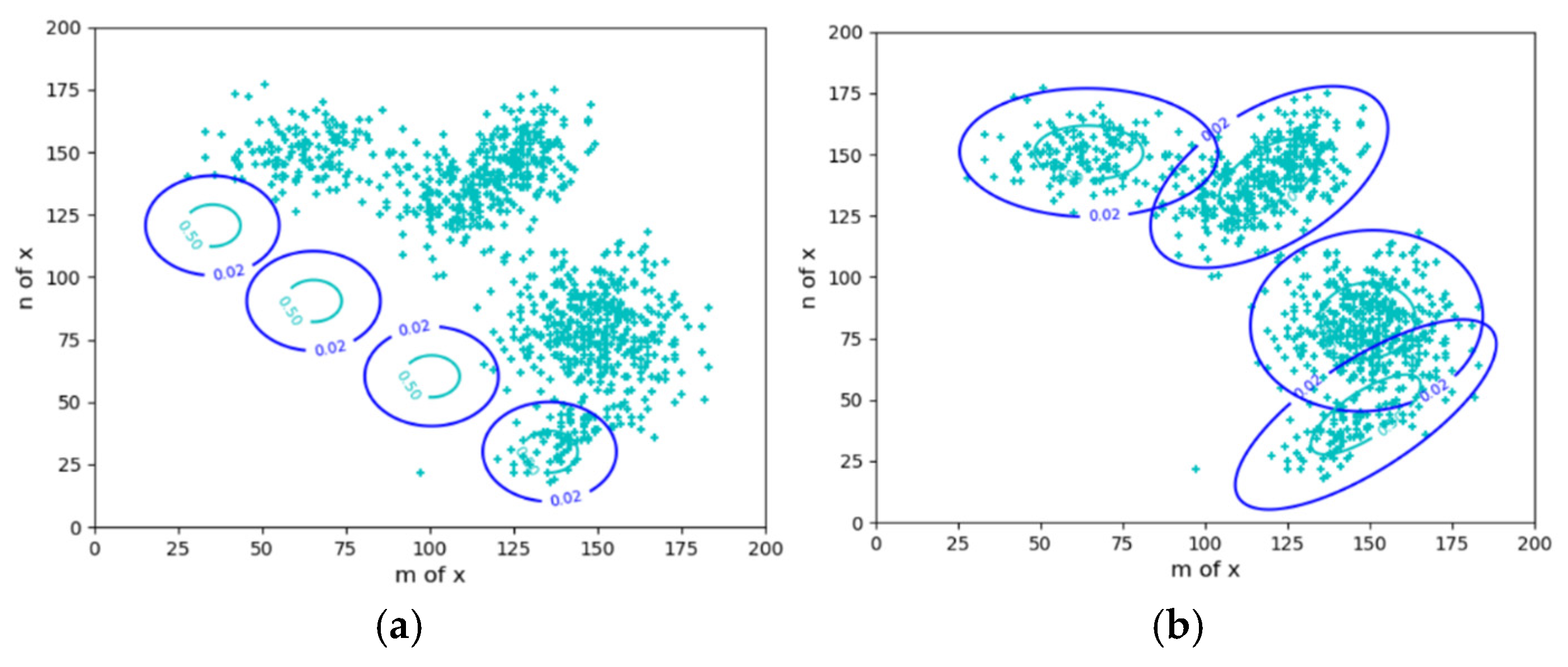
Figure 2.
Taking herding sheep as an example to illustrate the constraint control of uncertain events (the constraint condition is some fuzzy ranges). (a) Control starts; (b) Control ends.
Figure 2.
Taking herding sheep as an example to illustrate the constraint control of uncertain events (the constraint condition is some fuzzy ranges). (a) Control starts; (b) Control ends.
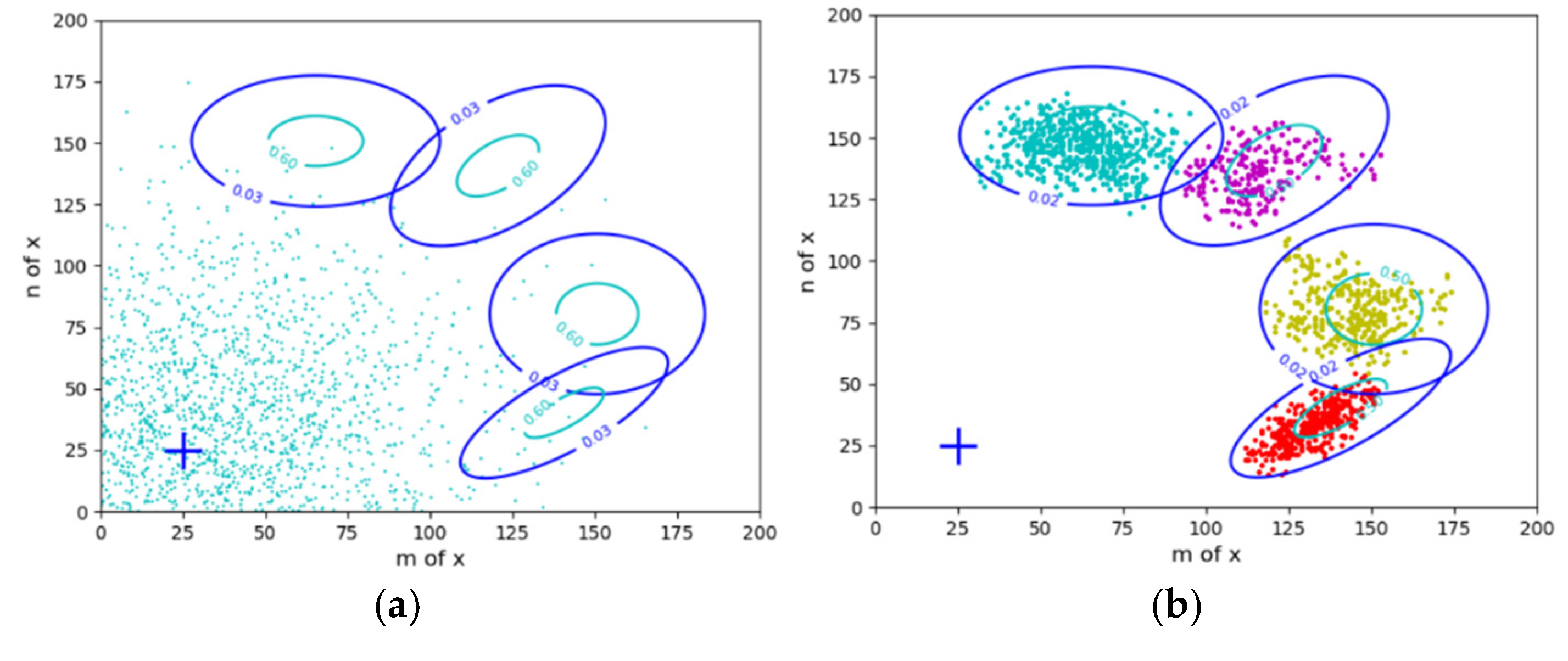
Figure 3.
The information rate-fidelity function R(G) for binary communication. Any R(G) function is a bowl-like function. There is a point at which R(G) = G (s = 1). For given R, two anti-functions exist: G-(R) and G+(R).
Figure 3.
The information rate-fidelity function R(G) for binary communication. Any R(G) function is a bowl-like function. There is a point at which R(G) = G (s = 1). For given R, two anti-functions exist: G-(R) and G+(R).
Figure 4.
Degeneracy gi is the microstate number of a molecule with energy ei.
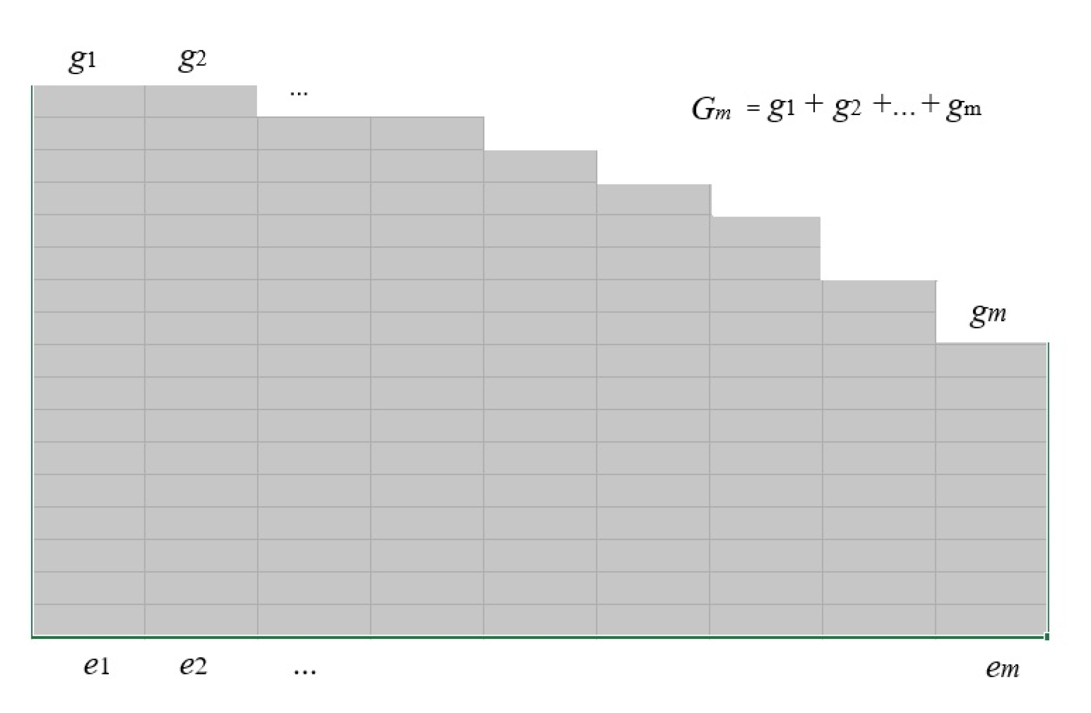
Figure 5.
The convergence process of the mixture model used by Neal and Hinton. After the true model’s mixture ratio was changed from 0.7:0.3 to 0.3:0.7, F’ and Q decreased in some steps. (a) The iteration starts; (b) iteration converges; (c) R, G, F’, and Q change in the iteration process.
Figure 5.
The convergence process of the mixture model used by Neal and Hinton. After the true model’s mixture ratio was changed from 0.7:0.3 to 0.3:0.7, F’ and Q decreased in some steps. (a) The iteration starts; (b) iteration converges; (c) R, G, F’, and Q change in the iteration process.

Figure 6.
A typical mixture model against the MFE principle. (a) The iteration starts; (b) Iteration converges; (c) R, G, F’, and Q change in the iteration process.
Figure 6.
A typical mixture model against the MFE principle. (a) The iteration starts; (b) Iteration converges; (c) R, G, F’, and Q change in the iteration process.
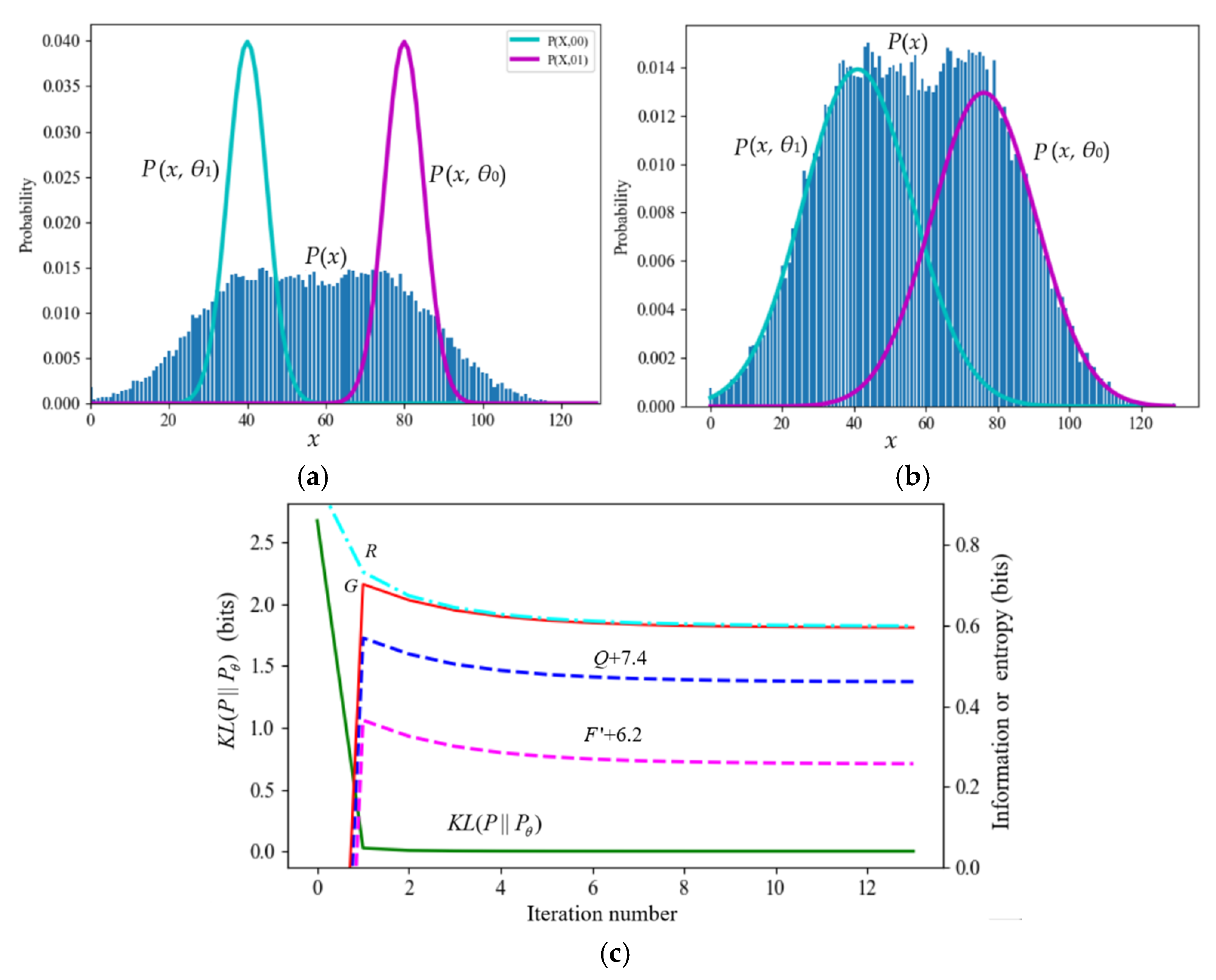
Figure 7.
The mixture model that is hard to converge. Hcross(Y) = –∑j P+1(yj)logP(yj) is the cross entropy. (a) The iteration starts; (b) the iteration converges; (3) the iteration process of the EM algorithm; (d) the iterative process of the E3M algorithm.
Figure 7.
The mixture model that is hard to converge. Hcross(Y) = –∑j P+1(yj)logP(yj) is the cross entropy. (a) The iteration starts; (b) the iteration converges; (3) the iteration process of the EM algorithm; (d) the iterative process of the E3M algorithm.
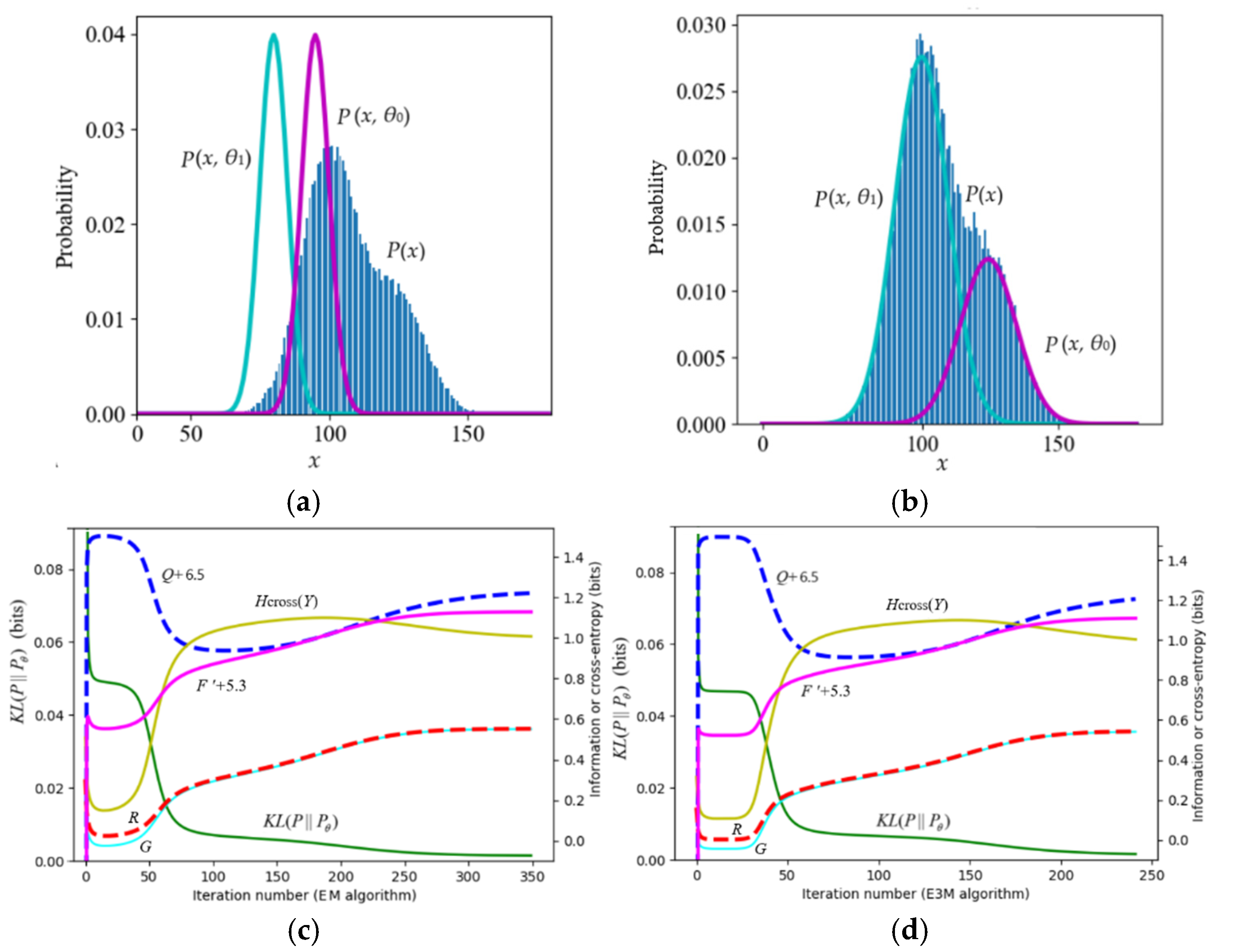
Figure 8.
Using the En algorithm to optimize the Shannon channel P(y|x). (a) Eight truth functions as the constraint; (b) the optimized P(y|x); (c) R, G and H(Y) change with the MID iteration.
Figure 8.
Using the En algorithm to optimize the Shannon channel P(y|x). (a) Eight truth functions as the constraint; (b) the optimized P(y|x); (c) R, G and H(Y) change with the MID iteration.
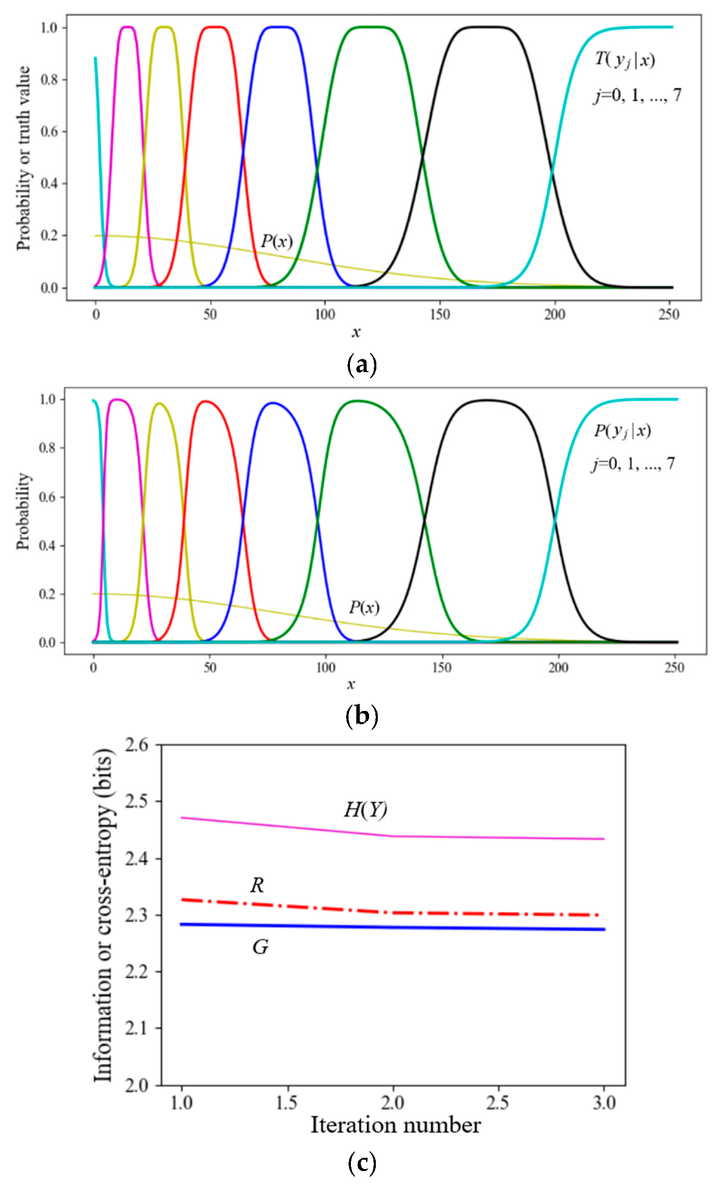
Figure 9.
A two-objective control task. (a) For the case with s=1; (b) for the case with s=5. P(x|βj, s) is a normal distribution produced by the action aj.
Figure 9.
A two-objective control task. (a) For the case with s=1; (b) for the case with s=5. P(x|βj, s) is a normal distribution produced by the action aj.
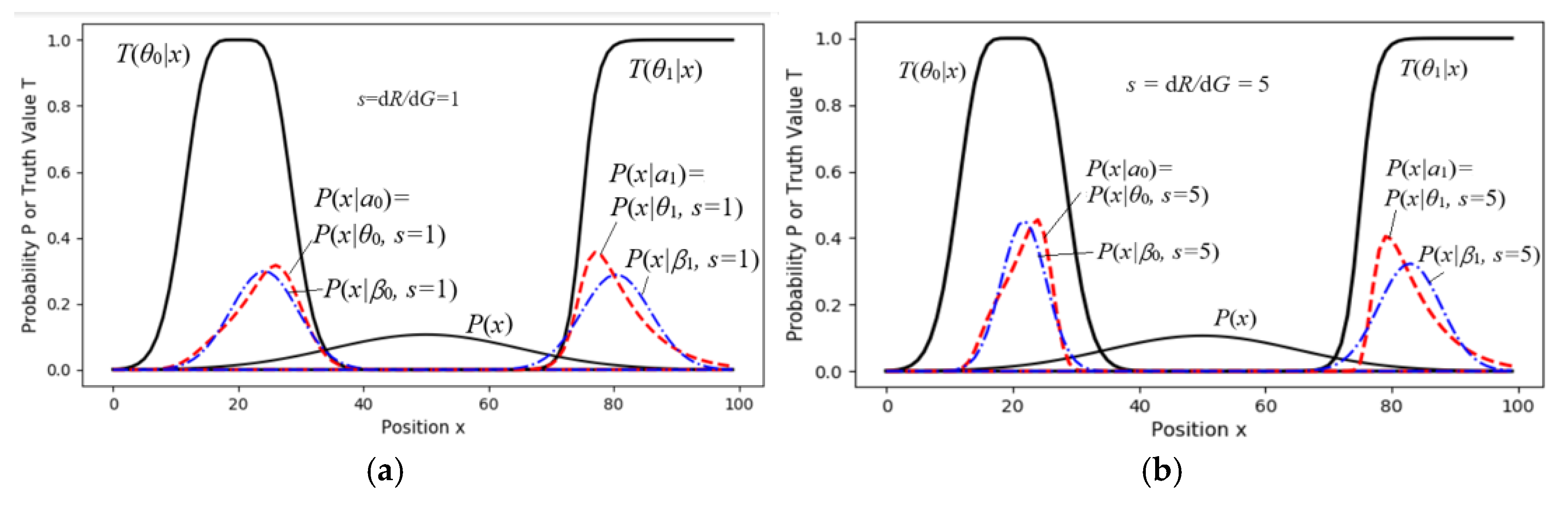
Figure 10.
The R(G) for constraint control. G slightly increases when s increases from 5 to 40, meaning s=5 is good enough.
Figure 10.
The R(G) for constraint control. G slightly increases when s increases from 5 to 40, meaning s=5 is good enough.
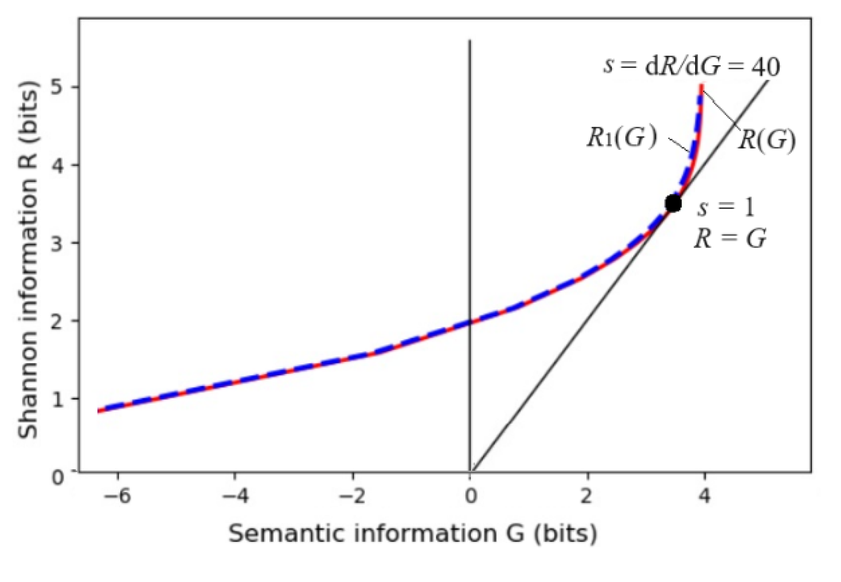

Table 1.
H(X|θj) increases when P(x|yj) is close to P(x|θj).
| x1 | x2 | x3 | x4 | H(X|θj) (bits) | |
| P(x|θj) | 0.1 | 0.4 | 0.4 | 0.1 | |
| P(x|yj) | 0 | 0.5 | 0.5 | 0 | log(10/4)= 1.32 |
| P(x|yj)=P(x|θj) | 0.1 | 0.4 | 0.4 | 0.1 | 0.2log(10)+0.8log(10/4)=1.72 |
Table 2.
Neal and Hinton’s mixture model example.
| True model’sParameters | Initialparameters | ||||||
| μ* | σ* | P*(y) | μ | σ | P(y) | ||
| y1 | 46 | 2 | 0.7 | 30 | 20 | 0.5 | |
| y2 | 50 | 20 | 0.3 | 70 | 20 | 0.5 | |
Table 3.
A mixture model whose F’ and Q decreased in the convergent process.
| The true model’sParameters | Initialparameters | |||||
| μ* | σ* | P*(Y) | μ | σ | P(Y) | |
| y1 | 40 | 15 | 0.5 | 40 | 5 | 0.5 |
| y2 | 75 | 15 | 0.5 | 80 | 5 | 0.5 |
Disclaimer/Publisher’s Note: The statements, opinions and data contained in all publications are solely those of the individual author(s) and contributor(s) and not of MDPI and/or the editor(s). MDPI and/or the editor(s) disclaim responsibility for any injury to people or property resulting from any ideas, methods, instructions or products referred to in the content. |
© 2025 by the authors. Licensee MDPI, Basel, Switzerland. This article is an open access article distributed under the terms and conditions of the Creative Commons Attribution (CC BY) license (http://creativecommons.org/licenses/by/4.0/).
Copyright: This open access article is published under a Creative Commons CC BY 4.0 license, which permit the free download, distribution, and reuse, provided that the author and preprint are cited in any reuse.


