
Submitted:
08 February 2025
Posted:
10 February 2025
You are already at the latest version
Abstract
Lung cancer is a major health issue and a leading cause of cancer-related mortalities globally. Early diagnosis is essential for improving survival rates, with biopsy as the gold standard for tissue analysis. While digital histopathology enhances image quality and precision, manual analysis is time-consuming for pathologists, creating a need for automated classification methods. This research starts with image preprocessing using an adaptive fuzzy filter and segmentation via a Modified Simple Linear Iterative Clustering (SLIC) algorithm. The Segmented images are input to the Deep Learning architectures like ResNet-50 (RN-50), ResNet-101 (RN-101), and ResNet-152 (RN-152). Features extracted from these ResNet variants are fused using a Deep Weighted Averaging- Based Feature Fusion (DWAFF) technique, resulting in fused features termed ResNet-X (RN-X). To further refine these features, Particle Swarm Optimization (PSO) and Red Deer Optimization (RDO) techniques are employed within the Selective Feature Pooling layer. The optimized features are then passed to a Classification Layer that implements classifiers including Support Vector Machine (SVM), Decision Tree (DT), Random Forest (RF), K-Nearest Neighbor (KNN), SoftMax Discriminant Classifier (SDC), Bayesian Linear Discriminant Analysis Classifier (BLDC), and Multilayer Perceptron (MLP). Performance is assessed using K-fold cross-validation with K values of 2, 4, 5, 8, 10, and the results are compared using standard performance metrics. RN-X features obtained from the proposed DWAFF technique, combined with the MLP classifier, achieved a peak accuracy of 98.68% when using segmentation and RDO in the feature selection layer with K=10.
Keywords:
SLIC Segmentation
; RN-X
; PSO
; RDO
; MLP
; Cross Validation
1. Introduction
Cancer is a complex set of diseases marked by uncontrolled growth and spread [1], unlike benign tumors, which remain localized, whereas malignant tumors invade and damage nearby tissues. Lung cancer is the leading type in men and the third in women, closely linked to smoking, and is the primary contributor to cancer associated mortality globally [2]. The WHO projects cancer will become the top global cause of death by 2020 [3], with lung cancer alone causing around 1.80 million deaths. Projections indicate that by 2035, lung cancer might contribute up to 60% of all cancer-related fatalities [4]. Early-stage cancers that are operable have a 5-year survival rate of approximately 34%, but for inoperable cases, the rate drops to under 10%. Lung cancer, which is predominantly classified into non-small cell lung carcinoma (NSCLC) and small cell lung carcinoma (SCLC) [5], shows varying characteristics. NSCLC, making up about 85% of cases, includes adenocarcinoma (ADC), squamous cell carcinoma (SCC), and large cell carcinoma (LCC). The remaining 15% are SCLC cases.
Histopathological examination identifies lung cancer subtypes through biopsy reports [6], crucial for accurate diagnosis and effective treatment planning [7]. Computer-Aided Diagnosis (CAD) systems support pathologists by providing automated assessments to prevent misclassification [8]. Advances in artificial intelligence (AI) have enhanced both the precision and effectiveness of histopathological slide analysis. This study centers on categorizing lung cancer biopsy images into two distinct categories, adenocarcinoma and benign using deep learning frameworks.
1.1. Contribution of the Work
The Major Contribution of this research work can be summarized as follows:
1. Histopathological images are preprocessed using an adaptive fuzzy filter and segmented using the Modified SLIC algorithm.
2. The segmented images are passed through deep learning models such as ResNet-50, ResNet-101, and ResNet-152 for feature extraction, followed by a proposed deep weighted averaging feature fusion technique to generate RN-X features.
3. The extracted features from the ResNet models and RN-X are input to a Selective Feature Pooling Layer, which leverages PSO and RDO optimization algorithms for feature selection.
4. Finally, the Classification Layer implements the classifiers such as SVM, DT, RF, KNN, SDC, BLDC, and MLP, evaluated using K-fold cross-validation with K values of 2, 4, 5, 8, and 10.
This study is organized as follows: Section 2 provides a review of recent research on lung cancer detection. Section 3 presents the methodology. Section 4 details the proposed deep weighted averaging feature fusion technique and discusses the Selective Feature Pooling Layer, incorporating PSO and RDO methods, along with the classification layer. Section 5 focuses on result comparisons. Finally, Section 6 highlights key findings and suggests directions for future research.
2. Review of Lung Cancer Detection
Over recent decades, various approaches have been proposed for automated detection, segmentation, and classification in histopathological images using machine learning (ML) and deep learning (DL). Anthimopoulos M et al. [9] developed a CNN with five convolutional layers using Leaky ReLU activation, average pooling, and three fully connected layers. Lizuka et al. [10] combined Inception v3 and an RNN to classify stomach and colon biopsies, incorporating regularization and augmentation for robustness. Wang et al. [11] used a CNN for lung cancer pathology, achieving 90.1% accuracy with Softmax activation. Gessert N et al. [12] explored multiresolution EfficientNet for skin sore classification. Liu Y et al. [13] applied wavelet-based denoising to address noise in histopathological images, achieving 94.37% accuracy on the BreakHis dataset.
Zhou Y et al. [14] designed a hierarchical model using SVM and SURF features, achieving 91.14% accuracy, but performance at 400X magnification needs improvement. Wang et al. [15] introduced FE-BkCapsNet, combining CNNs with CapsNet, yielding up to 94.52% accuracy. Aresta et al. [16] used DenseNet121, achieving 87% accuracy on the BACH 2018 dataset. Spanhol et al. [17] combined CNN predictions, achieving 84% accuracy on BreaKHis at 200X magnification, while Filipczuk et al. [18] focused on nuclei segmentation and trained several classifiers using 25 shape and texture features.
Nada Mobarak et al. [19] created CoroNet, a CNN based on Xception, achieving 88.67% accuracy for breast cancer detection on the CBIS-DDSM dataset. Teresa et al. [20] applied CNN models on the Bioimaging2015 dataset, segmenting images into 512×512-pixel patches, achieving up to 83.3% accuracy. Ahsan Rafiq et al. [21] proposed a three-CNN model for breast cancer classification, achieving 90.10% accuracy. Hameed et al. [22] fine-tuned VGG models and used an ensemble approach, outperforming individual models. Wang P et al. [23] achieved 96.19% accuracy using wavelet transforms and SVM with a genetic algorithm for feature selection.
3. Materials and Methods
This section offers an in-depth overview of the resources and methodologies employed in the classification of lung and colon cancers. The methodological framework of this study is illustrated in Figure 1.
3.1. Dataset Used
The LC25000 dataset, introduced in 2020 [24], contains 25,000 color images of five tissue types, expanded through augmentation from an original 1,250 cancerous images. Images were resized to 768 × 768 pixels and verified for HIPAA compliance. This study focuses on 5,000 benign and 5,000 adenocarcinoma lung cancer images. Adenocarcinoma originates in glandular cells and often spreads to the alveoli. Benign tissues, while non-cancerous, typically require surgical removal and biopsy to confirm their nature.
3.2. Image Preprocessing
Histopathological image analysis is crucial for assessing tumor characteristics, clinical staging, and predicting patient survival [25]. However, these images face challenges such as Complex Geometric Patterns and Textures, Critical Textural Features, Image Dimension and Resolution Variations, and Colour and Noise Issues. This study demonstrates that applying an adaptive fuzzy filter to resized images (224 × 224) enhances clarity by reducing noise and artifacts, resulting in more accurate diagnoses. The filtered images are then used for segmentation of the region of interest (ROI).
3.3. Modified SLIC Algorithm-Based Segmentation
A super pixel groups adjacent pixels that exhibit similar color, luminance, and texture properties to segment an image [26]. The SLIC algorithm allocates M initial seed points uniformly throughout the image. For an image with N pixels segmented into M super pixels, each super pixel contains N/M pixels. The separation between neighboring seed points is . The feature vector of the centroid is , combining the CIELAB color values and the pixel position . To enhance segmentation, the SLIC algorithm adjusts each centroid to the point with the minimal gradient in a 3x3 neighborhood. After initialization, it iteratively clusters pixels by assigning them to the nearest center and computing distances within a 2S x 2S neighborhood of each center. In SLIC algorithm, the measure of proximity between a candidate pixel and the centroid of a cluster is expressed as,
Here, denotes the centroid label, and denotes the pixel index in the 2S×2S neighborhood. represents spatial similarity, represents color similarity, and is the total similarity with a lower signifying higher similarity. The parameter , where denotes neighborhood size and indicates compact factor balancing and , typically ranges from 1 to 40. This paper introduces a modified SLIC algorithm that simplifies calculations using a 3-dimensional feature vector consisting of spatial co-ordinates and grayscale feature (. The distance between a candidate pixel and the cluster centroid is revised as follows:
Where denotes pixel similarity in grayscale values, represents the overall similarity between the cluster centroid and the pixel co-ordinates. The algorithm of the modified SLIC Super pixel Segmentation as follows:
The microscopic color cell image is initially transformed into a grayscale format. It is then randomly split into segments. Given the grayscale probability distribution , and multiple thresholds (where ), the entropy for these segments can be expressed as:
The multiple thresholds for ideal classification for each segment adhere to the principle of maximum entropy, as follows:
These thresholds are determined using a conditional iteration algorithm.
Using the optimal thresholds, the grayscale image is divided into intervals: , , . Transform each interval to with a contrast-enhancing function . The function is convex in and concave in , with turning point , where . is determined by using the least squares principle:
To simplify image processing, grayscale transformation is modeled by the function:
Here, . Varying , generates different transformation curves. A higher , improves gray equalization in the interval . By choosing appropriate and values regional balance and contrast can be enhanced, leading to a more evenly adjusted and contrasted image.
Initialize clustering centers using grid super pixels with side length , and assign labels.
Move each center to the location with the minimum gradient within its 3 x 3 neighborhood.
Calculate the similarity distance from each pixel to within a radius S which matches the circular shape of the cell image.
Set . If and is within range, update to , and assign the label to pixel .
Repeat steps 4 to 6 until clustering converges. Recalculate each cluster's mean grayscale and spatial features to update centers.
Merge isolated small super pixels using an adjacent merging strategy for improved fit and coherence.
Figure 2 shows the image progression: from the original to the filtered image, followed by Original SLIC Superpixel Segmentation, Modified SLIC Superpixel Segmentation, and finally, the Modified SLIC result for the Adenocarcinoma Class (ACA).
4. Deep Feature Extraction
Deep learning networks are powerful but face challenges like saturation, accuracy degradation, and vanishing or exploding gradients. Architectures like ResNet-50 (RN-50), ResNet-101 (RN-101), and ResNet-152 (RN-152) address these issues using residual learning and identity mapping [27]. It uses shortcut connections that helps mitigate the vanishing gradient problem and prevents overfitting [28]. The mapping function as shown in Figure 3 is expressed as:
In Table 1, A, B, C, and D represent the number of blocks in the first, second, third, and fourth stages of the ResNet versions, respectively.
The ResNet architecture configurations consist of different stages that are stacked across various ResNet versions, resulting in a 1D feature vector with 2048 elements for each image as shown in Figure 4.
4.1. Proposed DWAFF Technique for ResNet-X Features
This study proposes a Deep Weighted Averaging based Feature Fusion (DWAFF) technique. In this method, ResNet variants are evaluated, and weights are assigned to their feature vectors based on performance. By prioritizing contributions from each architecture, weights (ranging from 0 to 1) are adjusted in increments of 0.1 through trial and error. The final fused feature set for each image is computed using the weighted sum of the features as follows:
The optimal weight combination for feature fusion was determined using K-fold Cross Validation on the dataset for each architecture - RN-50, RN-101, and RN-152, across various K values of 2, 4, 5, 8, and 10, as summarized in Table 7. Among these, ResNet 152 demonstrated highest accuracy followed by ResNet 101 and ResNet 50. The weight values for the architecture were chosen through a trail-and-error method, constrained to lie between 0 and 1, with their sum equal to 1. The best performing combination was identified as 0.45 for RN-152 (), 0.35 for RN-101 (), and 0.20 for RN-50 (). These weights were subsequently applied to fuse features using Equation 11. Additionally, the mean value of the normal class is added to the normal features, and the mean value of the abnormal class is added to the abnormal features, enhancing class separation, and improving classification. The equation for generating DWAFF-based RN-X features is given by:
For Normal cases,
For Abnormal cases,
In this context, , denotes the features extracted per image, represents the image index, for the normal class and for the abnormal class, is the average of mean values from all three ResNet variants for normal images, while represents the same abnormal images. The algorithm for the proposed DWAFF technique for ResNet X features is shown below:
Algorithm 1
Step 01: Extract Features
Extract feature vectors for each image from ResNet-50, ResNet-101, and ResNet-152.
Store the feature vectors: ResNet-50_feature [i, j], ResNet-101_feature [i, j], and ResNet-152_feature [i, j], where and .
Step 02: Perform K-Fold Cross Validation
For each K value (2, 4, 5, 8, 10):
Split the dataset into K folds.
Train the classifiers on the dataset set split.
Evaluate performance of the classifiers using performance metrics.
Step 03: Set Initial Weight Range
Initialize a range of possible weights , and based on the trial-and-error method, such that their sum must be equal to 1 according to the results obtained in Table 7 after K-fold Cross Validation.
Step 04: Identify Optimal Weights
For each weight combination, calculate the average performance across the K-folds.
Select the weight combination that achieves the highest average performance.
Optimal weights are identified as, 0.45 for ResNet-152 (), 0.35 for ResNet-101 (), and 0.20 for ResNet-50 ().
Step 05: Compute Mean Values
Compute and , across all three ResNet variants.
Step 06: Fuse Features for Final Feature Set
For Normal cases (): Fuse features of normal cases, Using Equation 12.
For Abnormal cases (): Fuse features of abnormal cases, Using Equation 13.
Step 07: Output Final Fused Features
The final fused feature set for both normal and abnormal cases, which is a ResNet-X features are used for subsequent classification tasks.
4.2. Statistical Analysis
To enhance cancer classification accuracy with a reduced number of features, statistical measures play a crucial role in further analysis. The extracted features from ResNet-50, ResNet-101, ResNet-152, and the fused features from ResNet-X are analyzed by calculating statistical metrics such as Mean, Variance, Skewness, Kurtosis, Pearson Correlation Coefficient (PCC), and Canonical Correlation Analysis (CCA). These measures help assess how effectively the features capture lung cancer characteristics in both cancerous and non-cancerous data.
Table 2 presents the statistical parameters for the ResNet-50, ResNet-101, ResNet-152, and DWAFF-ResNet-X architectures for Normal (N) and Abnormal (ACA) cases. DWAFF-ResNet-X shows the best average performance with the highest mean values for both N (0.453891) and ACA (0.453709), outperforming the ResNet models, whose performance improves with depth. In terms of variance, DWAFF-ResNet-X has the lowest values (N: 0.380702, ACA: 0.444597), indicating more consistent performance compared to the higher variances in ResNet models, especially in ACA. For skewness, DWAFF-ResNet-X (N: 3.767961, ACA: 4.486885) shows a more symmetrical performance distribution, whereas ResNet models have higher skewness, indicating more inconsistent results. Kurtosis is also lower for DWAFF-ResNet-X (N: 21.14865, ACA: 33.4781), reflecting fewer extreme outliers than ResNet models, which have higher kurtosis values. PCC is highest in DWAFF-ResNet-X (N: 0.938638, ACA: 0.944338), indicating stronger alignment between predictions and outcomes compared to ResNet models. CCA also improves with model depth, with DWAFF-ResNet-X showing the highest CCA for ACA (0.8816). The Dice Coefficient values indicate the performance of the models in segmentation tasks. ResNet-50 shows moderate performance, with slightly better accuracy for normal cases. ResNet-101 outperforms ResNet-50, especially for normal cases. ResNet-152 demonstrates significant improvement, achieving higher accuracy for both normal and abnormal cases. DWAFF-ResNet-X delivers the best performance, with the highest Dice Coefficients for both normal and abnormal cases, making it the most effective model.
Figure 5 shows a scatterplot matrix of features extracted from ResNet-50, ResNet-101, ResNet-152, and ResNet-X. Normal and abnormal features are represented as RN-50-N/RN-50-ACA, RN-101-N/RN-101-ACA, RN-152-N/RN-152-ACA, and RN-X-N/RN-X-ACA, respectively. The scatterplots reveal nonlinear relationships between normal and abnormal features, with dense clusters near one axis and sparser distributions elsewhere. Significant overlaps between the classes are evident, particularly in ResNet-50 and ResNet-101, complicating classification. However, ResNet-152 and ResNet-X show better class separation, with abnormal features appearing more dispersed and normal features more clustered. This improved separation suggests that ResNet-X and ResNet-152 features may support more accurate classification. While overlaps persist across all models, careful feature selection could enhance classification performance, particularly with nonlinear classifiers.
The violin plot shown in Figure 6 illustrates the data distributions of features extracted by ResNet models (ResNet-50, ResNet-101, ResNet-152, and ResNet-X) for normal (N) and abnormal (ACA) classes. ResNet-50 shows minimal variation and significant overlap, indicating poor class differentiation. ResNet-101 captures more variation but still has considerable overlap, limiting separability. ResNet-152 demonstrates distinct distributions with reduced overlap, suggesting better feature separability. ResNet-X exhibits the widest distributions and more pronounced separation, making it the most promising for classification tasks. Feature differentiation improves progressively from ResNet-50 to ResNet-X.
4.3. Selective Feature Pooling Layer
The Selective Feature Pooling Layer is designed to condense the features of histopathological images into compact feature vectors, enhancing classifier performance and promoting high generalization capability. In lung cancer diagnosis [29], these techniques enhance accuracy by using Bio-inspired Optimization algorithms like PSO and RDO.
4.3.1. Particle Swarm Optimization (PSO)
The Particle Swarm Optimization (PSO), first proposed by Kennedy and Eberhart in 1995, mimics bird flock behavior to optimize problems. It begins by initializing particles and defining essential parameters [30]. The algorithm for the PSO with particle position and velocity updates are given below.
Algorithm 2: PSO
Initialization:
- Maximum iteration count: - Inertia weight range: (, )
- Acceleration coefficients: c1, c2
- Set the position of each particle randomly: ------ (14)
- Set the velocity of each particle randomly: ------ (15)
- Initialize best position for an individual particle as and = the best of all .
for k = 0 to k_max-1 do:
for i = 1 to n do:
Calculate the inertia weight: ------ (16)
Update the velocity: ------ (17)
Update the position: ------ (14)
Update if the new position surpasses the previous Update if the new surpasses the current Output the final as the optimal solution.
In this study, the following parameter values are selected through an iterative process of experimentation and refinement: Inertia weight (wi) - between 0.45 and 0.9, Maximum number of iterations - between 100 and 1000, Random values (r1 and r2) - set to 0.85, Cognitive component (c1) and social component (c2) - between 1.0 and 2.0.
4.3.2. Red Deer Optimization (RDO)
Red Deer Optimization (RDA), introduced in 2016 [31], emulates the courtship rituals of Scottish Red Deer. The algorithm starts with an initial population of "red deer" (RDs). The best RDs, called "RD males," are split into "commanders" and "stags" based on their initial performance. Commanders and stags compete for harems, with successful stags potentially becoming commanders. Commanders pair with hinds in their harems and others, while stags mate with nearby hinds. This process blends exploration and exploitation, generating new solutions and allowing weaker solutions to evolve. In terms of dimensionality reduction, RDA uses this evolutionary process to refine and optimize the solution space by iteratively improving and filtering candidate solutions. The process for RDO follows here:
Algorithm 3: RDO
Initial Population:
-Define the solution space with dimensions:
Here, represents the array size, set to 50. Each component corresponds to a vector of values for each of the 50 images, as defined by the equation below.
-Initialize a random population of red deer (RDs).
Roaring Stage:
-For each male RD:
--Calculate the new position based on fitness function (FF) value using.
Here, UL and LL represent the maximum and minimum boundaries of the search region, respectively. The factors a1, a2 and a3 are randomly selected from a uniform distribution between zero and one.
--Update the RD position and evaluate its fitness.
--Promote successful RDs to commander status if they show improved fitness.
Competition Stage:
-Each commander competes with random stags:
--Compute new positions:
--Select the position with the best fitness function (FF) to update the commander status.
Harem Creation Phase:
-For harems with:
--A commander and several hinds based on the commander's fitness.
--Calculate the number of hinds as:
--Stags do not participate in harems.
Mating Phase:
-Commander Mating Within Harems: Each commander mates with a proportion () of its hinds
-Commander Expansion Beyond Harems: Commanders mate with a percentage () of hinds from other harems. The parameter () ranges from 0 to 1.
-Stag Mating: Stags mate with the closest hind.
Offspring Creation:
-Generate new offspring using:
Where is the new offspring RD, c is randomly chosen between 0 and 1. For -Stage mating, replace Com with Stag.
Next Generation Solution:
-Retain a percentage of the best male RDs.
-Select hinds and offspring for the next generation using fitness-based methods.
Stopping Criterion:
-RDO's stopping criteria include:
1. Fixed number of iterations. 2. Achievement of a quality threshold. 3. Exceeding a time limit.
The parameters of the RDO algorithm are described in the following Table 3.
4.4. Entropy Based on Statistical Analysis
In biomedical applications, entropy has emerged as a widely used approach. When applied to feature selection, entropy-based techniques assess the relevance and significance of selected features by quantifying the amount of information each feature contributes to predicting the target variable. In this study, the selected features from the normal and abnormal classes are evaluated using Approximate Entropy, Shannon Entropy, and Fuzzy Entropy.
4.4.1. Approximate Entropy
Approximate Entropy is a statistical method for measuring the regularity and unpredictability of variations in time-series data [32]. It calculates the difference between the natural logarithms of repeating patterns of length n and n+1, using the formula:
Here, is the input feature length and is the mean of all ranges. is given as,
In the input vector of length , represents the number of features. A higher approximate entropy value indicates that the input feature vectors are more complex and less predictable.
4.4.2. Shannon Entropy
The Shannon Entropy of a random variable S containing values is determined by,
Here, represent the probability function. If the entropy score is high, it means that the outcome is hard to predict because it is uncertain.
4.4.3. Fuzzy Entropy
Fuzzy Entropy, a statistical method used to quantify the uniformity of input feature vectors [33]. It is defined by the following formula:
Here, , and represents the membership value of the fuzzy set and M is the total number of data points.
Table 4 compares the feature selection methods PSO and RDO in terms of entropy based statistical parameters such as Approximate Entropy, Shannon Entropy, and Fuzzy Entropy. Approximate Entropy measures the regularity and predictability of time-series data. PSO, with lower Approximate Entropy values (1.2385 for N and 1.7816 for ACA) compared to RDO (2.0123 for N and 2.4893 for ACA), indicates more regularity and less complexity. RDO, with higher values, suggests greater variability and less predictability, possibly capturing more nuanced features. Shannon Entropy reflects uncertainty or information content. RDO's higher values (5.0821 for N and 5.8982 for ACA) show greater complexity and feature diversity compared to PSO's lower values (3.8523 for N and 4.9891 for ACA), which suggest more structured data but less feature variety. Fuzzy Entropy, which measures complexity in a fuzzy system, is higher for RDO (0.7283 for N and 0.9182 for ACA), indicating more ambiguity in feature relationships. PSO's lower values (0.4862 for N and 0.5231 for ACA) suggest clearer, better-defined relationships with less uncertainty.
4.5. Classification Layer
Classifiers are essential for categorizing data, aiming for high accuracy and minimal errors while balancing computational complexity. This study utilized the following classifiers in the classification layer part of the ResNet architectures:
4.5.1. Support Vector Machine (SVM)
SVM is a set of supervised learning methods utilized for categorization, prediction, and anomaly detection, due to its scalability and high performance [34]. Linear SVMs use a maximum-margin hyperplane (either hard or soft margin), while non-linear SVMs apply kernel functions for classification. The Hyperplane is determined by,
Subject to Here is the vector that is perpendicular to the hyperplane, is a data point, is a scalar, and are slack variables penalizing misclassifications. The decision function is . Various kernels such as linear, polynomial, RBF, and sigmoid are used in SVMs. This study uses the SVM-RBF kernel to enhance classification accuracy.
4.5.2. Decision Tree (DT)
A Decision Tree (DT) is a flexible algorithm for categorization and regression, using a tree structure with decision nodes based on features and leaf nodes for outcomes [34]. Starting at the root, the tree is traversed to make predictions. Nodes split data by feature and threshold, while leaf nodes provide final predictions. Key metrics for node impurity include:
where represents the feature, denotes the collection of instances at the node, and is the subset of instances with feature has the value . Gini Impurity is given as follows:
where is the frequency of class k and is the number of classes. The objective is to find the feature and threshold that minimize impurity, with the optimal split S given by:
4.5.3. Random Forest (RF)
The Random Forest algorithm excels in image classification due to its accuracy and robustness [35]. It uses multiple independent decision trees, with key parameters including the number of trees and features considered by each tree. The final prediction is made by combining the decision from all trees, with the formula:
where is the final prediction, D is the number of trees, is the prediction from the tree, and is the class label.
4.5.4. K-Nearest Neighbor (KNN)
The KNN algorithm determines the category of a data point by comparing its distance to the K closest points in the training data and assigns it to the class that appears most frequently among these neighboring points. It requires no separate training phase and uses the entire dataset for classification. In Weighted KNN, neighbors are weighted inversely to their distance from the query point [36]. The distance between two points and , is calculated as:
In weighted KNN, is given by , with a small constant added to avoid division by zero. The classification of a query point is determined by the most common class among its K closest neighbors,
Here represent the set of K nearest neighbors, is the class label of neighbor and is the indicator function. This study uses k=5 with mixed Euclidean distance to improve classification accuracy by weighing closer neighbors more heavily.
4.5.5. Softmax Discriminant Classifier (SDC)
The SDC identifies and verifies the class of a test sample [37], by measuring its distance to training samples within each class. Given a training set, , where contains samples from class q, with . The samples used for testing are presumed to be , then SDC is defined as,
where measures the distinction between the test sample and class j. A penalty cost λ > 0 is applied. If v and vn are similar, and y belongs to class i, is close to zero, making approach its maximum value.
4.5.6. Multi-Layer Perceptron (MLP)
Multilayer Perceptrons (MLPs) are used for function approximation tasks like regression [38]. The MLP structure consists of an input layer with n nodes, an intermediate layer, and an output layer. Input-output pairs are denoted as , where is the input vector and is the target output, the output of the k-th hidden node is computed as:
The final output is given by,
Where represent the number of hidden units, θ denote the bias at the output layer and be the weight connecting the k-th hidden unit to the output layer. This configuration results in (n+2) j+1 connections. The cost function for training the MLP is:
In this study, a 3-layer architecture was utilized, recognized for its effectiveness in approximating continuous functions [39].
4.5.7. BLDC
The Bayesian Linear Discriminant Classifier (BLDC) employs the Fisher linear discriminant alongside Bayes decision rule to reduce the probability of classification errors [40], effectively regularizing high-dimensional signals and enhancing computational efficiency. In Bayesian regression, the target a is defined as:
where q is the weight vector and n is white gaussian noise. The weighted likelihood function is:
Here, is the target value, is the matrix of training feature vectors, D combines and . is the inverse noise variance, and is the number of training samples. The prior distribution is given by:
where N is the feature size, denotes the (N+1) dimensional regularization diagonal matrix, represented as follows:
The posterior distribution of s is:
This posterior distribution is Gaussian with covariance matrix H and mean vector U:
For predictive variation of , the distribution on the regression target is:
This Predictive distribution is also gaussian with mean and variance as follows:
5. Results and Discussion
This study uses deep learning-based feature extraction and feature fusion techniques along with feature selection using PSO and RDO for categorizing histopathological images of lung cancer on a Windows 11 workstation with an AMD Ryzen 7 5700G processor and integrated Radeon Graphics, running MATLAB 2018a.
5.1. Training and Testing of the Classifiers
In this study, K-fold cross-validation is used for classification. For instance, with K=10, the dataset is divided into 10 equal segments, where each segment is used once as the test set and the remaining nine as the training set. Performance metrics are average across iterations. Different K values such as 2, 4, 5, 8, and 10 were evaluated. The training data is partitioned into smaller batches, and classifiers such as SVM, DT, RF, KNN, and BLDC are trained iteratively on these smaller batches, while MLP and SDC are trained directly over epochs. After each epoch, performance is evaluated on both training and validation sets, and accuracy is recorded. Finally, the training and validation accuracies are plotted to visualize performance over epochs. Training stops after a maximum of 15 epochs or when accuracy levels suggest potential overfitting. Testing ends once all batches are processed. Higher accuracy and lower error rates indicate better classifier performance. Table 5 lists the parameters selected for various classifiers, chosen through trial and error, with a maximum of 15 epochs to prevent overfitting.
5.2. Standard Benchmark Metrics of the Classifiers
In this study, several transfer learning models are assessed using a confusion matrix. The evaluation process involves using 90% of the input features for training and setting aside 10% for testing. In the context of lung cancer detection, the clinical scenarios related to the confusion matrix are defined as follows: True Positive (TP): Correct identifying a patient as Benign. True Negative (TN): Correct identifying of a patient as Adenocarcinoma. False Positive (FP): Incorrectly classifying an Adenocarcinoma patient as Benign. False Negative (FN): Misclassifying a Benign patient as Adenocarcinoma. The performance of the classifiers is evaluated using metrics such as Accuracy, Error Rate, F1 Score, Matthews Correlation Coefficient (MCC), Jaccard Index, G-Mean, and Kappa. The mathematical formulations for these metrics are detailed in Table 6.
5.3. Performance Analysis of the Classifiers in Terms of Accuracy for Different K Values
In this study, the performance of seven classifiers—SVM, KNN, Random Forest, Decision Tree, Softmax Discriminant, MLP, and BLDC—was evaluated for cancer image classification across K values of 2, 4, 5, 8, and 10, as shown in Table 7.
In the first scenario, without segmentation, the ResNet-X based feature fusion technique combined with an MLP model achieved an accuracy of 58.610% at K=2 and 63.150% at K=4. The ResNet-50 based feature extraction with the MLP model reached its highest accuracy of 65.230% at K=5, while the ResNet-152 based feature extraction with the MLP model attained a peak accuracy of 68.783% at K=8. Additionally, the ResNet-X based feature fusion technique combined with the MLP model achieved a top accuracy of 69.610% at K=10. In the second scenario, with segmentation, ResNet-152 based feature extraction combined with the MLP model achieved 66.920% accuracy at K=2 and 74.380% at K=5. The ResNet-101 based feature extraction with the MLP reached 72.910% at K=4, while the ResNet-50 based feature extraction with the MLP peaked at 83.730% at K=8. Additionally, the ResNet-X based feature fusion technique combined with the MLP attained a top accuracy of 86.460% at K=10.
In the third scenario, with segmentation and Feature selection, applying PSO for feature selection resulted in a ResNet-50 based feature extraction with the MLP achieving 72.250% accuracy at K=2. The ResNet-152 based feature extraction with the MLP attained 76.432% at K=4, 79.490% at K=5, and 93.508% at K=8, while the ResNet-X based feature fusion technique combined with the MLP reached 96.490% at K=10. Using RDO for feature selection, the ResNet-50 based feature extraction with the MLP achieved 77.980% accuracy at K=2. The ResNet-152 based feature extraction with the MLP reached 87.240% at K=5, while the ResNet-X based feature fusion technique combined with the MLP recorded 82.810% at K=4, 94.531% at K=8, and 98.680% at K=10. Across all scenarios, ResNet-X based feature fusion technique combined with the MLP consistently achieved the highest accuracy, demonstrating its effective deep-weighted averaging feature fusion capabilities.

Table 7.
Performance analysis of the Classifiers for all three cases in terms of Accuracy.
| DL model with Classifiers | Without Segmentation and FS | With Segmentation only | With Segmentation and PSO FS | With Segmentation and RDO FS | ||||||||||||||||
|---|---|---|---|---|---|---|---|---|---|---|---|---|---|---|---|---|---|---|---|---|
| K = 2 | K = 4 | K = 5 | K = 8 | K = 10 | K = 2 | K = 4 | K = 5 | K = 8 | K = 10 | K = 2 | K = 4 | K = 5 | K = 8 | K = 10 | K = 2 | K = 4 | K = 5 | K = 8 | K = 10 | |
| ResNet-50-SVM | 53.700 | 59.324 | 62.990 | 62.500 | 57.200 | 65.820 | 65.100 | 72.270 | 73.703 | 74.350 | 65.820 | 72.983 | 71.633 | 82.872 | 90.110 | 73.230 | 77.082 | 83.140 | 85.803 | 89.840 |
| ResNet-50-DT | 54.500 | 56.860 | 60.160 | 57.063 | 67.060 | 60.830 | 64.780 | 71.520 | 70.603 | 73.910 | 61.380 | 71.270 | 73.173 | 83.600 | 91.290 | 72.250 | 78.922 | 78.382 | 85.681 | 90.630 |
| ResNet-50-RF | 56.070 | 59.164 | 62.630 | 59.914 | 68.230 | 62.960 | 66.213 | 68.260 | 72.790 | 79.420 | 62.960 | 74.150 | 74.743 | 86.920 | 93.110 | 75.830 | 79.040 | 82.422 | 87.141 | 91.140 |
| ResNet-50-KNN | 53.690 | 59.650 | 62.370 | 66.540 | 65.540 | 61.530 | 68.033 | 66.473 | 71.100 | 72.790 | 61.530 | 73.570 | 65.430 | 87.500 | 89.840 | 73.590 | 75.950 | 78.642 | 84.120 | 93.350 |
| ResNet-50-SDC | 55.190 | 60.450 | 64.070 | 68.445 | 59.790 | 59.730 | 69.733 | 70.573 | 77.862 | 80.730 | 71.100 | 72.790 | 75.260 | 91.012 | 92.750 | 77.760 | 76.302 | 82.812 | 85.810 | 93.750 |
| ResNet-50-BLDC | 51.420 | 56.510 | 57.430 | 57.950 | 58.150 | 63.590 | 63.404 | 64.490 | 74.673 | 77.090 | 65.950 | 65.230 | 65.883 | 78.840 | 87.100 | 73.170 | 73.700 | 77.220 | 83.332 | 90.880 |
| ResNet-50-MLP | 53.710 | 61.704 | 65.230 | 62.440 | 58.700 | 66.850 | 71.110 | 72.363 | 83.730 | 81.250 | 72.250 | 74.773 | 77.082 | 92.181 | 94.010 | 77.980 | 79.752 | 85.160 | 91.731 | 95.310 |
| ResNet-101-SVM | 54.900 | 61.270 | 61.220 | 67.580 | 64.330 | 63.220 | 64.524 | 66.103 | 77.990 | 69.760 | 63.590 | 70.893 | 68.163 | 86.713 | 89.960 | 76.590 | 80.800 | 75.130 | 89.451 | 90.760 |
| ResNet-101-DT | 56.620 | 61.820 | 62.760 | 61.440 | 60.940 | 60.830 | 67.210 | 64.980 | 73.960 | 76.110 | 61.340 | 71.550 | 64.230 | 80.210 | 90.620 | 73.373 | 76.942 | 76.170 | 82.950 | 91.670 |
| ResNet-101-RF | 57.310 | 62.350 | 63.970 | 63.670 | 65.130 | 62.000 | 69.010 | 66.000 | 78.640 | 74.020 | 62.000 | 72.500 | 65.890 | 82.292 | 91.670 | 74.090 | 77.932 | 78.902 | 89.711 | 93.350 |
| ResNet-101-KNN | 54.242 | 60.960 | 56.330 | 60.430 | 67.969 | 64.010 | 70.380 | 67.380 | 73.050 | 80.980 | 64.750 | 65.310 | 73.153 | 86.761 | 87.760 | 74.590 | 80.270 | 81.572 | 83.592 | 90.230 |
| ResNet-101-SDC | 58.450 | 62.990 | 63.770 | 66.570 | 60.680 | 64.520 | 71.910 | 68.360 | 80.790 | 82.550 | 68.700 | 71.383 | 77.342 | 89.321 | 93.490 | 75.010 | 78.390 | 83.752 | 90.760 | 97.130 |
| ResNet-101-BLDC | 53.700 | 56.720 | 56.249 | 56.774 | 54.450 | 59.680 | 63.530 | 67.970 | 75.000 | 81.310 | 60.830 | 63.570 | 68.040 | 79.560 | 90.360 | 69.240 | 73.113 | 75.520 | 82.620 | 89.320 |
| ResNet-101-MLP | 58.610 | 63.150 | 64.490 | 66.780 | 60.530 | 66.420 | 72.910 | 72.581 | 82.940 | 84.120 | 70.590 | 74.610 | 78.130 | 92.441 | 94.530 | 77.830 | 76.432 | 84.640 | 92.906 | 96.350 |
| ResNet152-SVM | 56.090 | 61.080 | 60.414 | 66.123 | 61.360 | 63.580 | 66.410 | 71.750 | 77.150 | 74.480 | 66.420 | 68.050 | 69.013 | 84.900 | 93.220 | 74.290 | 76.240 | 81.250 | 82.560 | 92.370 |
| ResNet152-DT | 53.840 | 62.870 | 61.704 | 62.714 | 55.970 | 64.660 | 68.820 | 66.410 | 75.062 | 73.370 | 64.520 | 70.960 | 71.873 | 88.541 | 90.110 | 70.890 | 80.080 | 81.672 | 82.352 | 92.570 |
| ResNet152-RF | 57.950 | 63.090 | 62.990 | 68.160 | 63.670 | 65.840 | 70.060 | 68.490 | 71.873 | 80.070 | 68.100 | 71.350 | 76.822 | 89.190 | 92.180 | 71.093 | 81.900 | 82.820 | 85.970 | 93.030 |
| ResNet152-KNN | 54.940 | 62.000 | 57.120 | 60.804 | 66.270 | 61.380 | 65.853 | 61.704 | 70.320 | 81.510 | 63.580 | 69.530 | 73.953 | 79.820 | 91.460 | 72.340 | 81.380 | 84.250 | 86.983 | 92.310 |
| ResNet152-SDC | 56.190 | 60.690 | 63.386 | 65.500 | 67.550 | 65.950 | 69.760 | 73.940 | 74.480 | 82.090 | 68.100 | 75.690 | 73.960 | 92.190 | 93.750 | 73.563 | 82.170 | 85.160 | 92.748 | 95.960 |
| ResNet152-BLDC | 55.930 | 55.810 | 59.444 | 58.840 | 59.340 | 59.830 | 64.000 | 66.670 | 72.620 | 75.770 | 63.220 | 63.900 | 70.920 | 79.750 | 93.230 | 69.273 | 78.970 | 76.885 | 82.690 | 86.710 |
| ResNet152-MLP | 56.250 | 61.460 | 64.157 | 68.783 | 57.880 | 66.920 | 72.010 | 74.380 | 78.902 | 85.420 | 70.480 | 76.432 | 79.490 | 93.508 | 94.520 | 77.100 | 82.550 | 87.240 | 93.435 | 97.660 |
| ResNet-X-SVM | 57.410 | 56.120 | 57.670 | 67.300 | 56.780 | 62.100 | 66.703 | 68.230 | 70.703 | 73.300 | 66.280 | 66.490 | 70.813 | 82.812 | 91.670 | 77.410 | 80.110 | 77.862 | 89.650 | 91.640 |
| ResNet-X-DT | 54.900 | 59.830 | 61.460 | 63.480 | 60.020 | 61.080 | 71.650 | 66.970 | 72.530 | 76.690 | 64.010 | 73.390 | 66.670 | 85.680 | 88.600 | 69.730 | 76.170 | 78.252 | 84.770 | 92.180 |
| ResNet-X-RF | 56.120 | 62.100 | 63.150 | 64.390 | 64.800 | 64.660 | 72.460 | 71.093 | 77.410 | 77.580 | 66.920 | 74.800 | 70.633 | 87.761 | 92.190 | 70.543 | 79.920 | 84.892 | 86.391 | 94.010 |
| ResNet-X-KNN | 56.860 | 55.514 | 58.760 | 60.610 | 54.850 | 61.340 | 67.650 | 67.153 | 77.990 | 78.650 | 68.690 | 70.303 | 68.670 | 88.801 | 91.660 | 71.240 | 77.790 | 78.772 | 89.871 | 93.220 |
| ResNet-X-SDC | 58.450 | 60.960 | 62.760 | 67.690 | 68.930 | 64.750 | 65.450 | 73.180 | 80.210 | 83.850 | 70.080 | 75.130 | 70.633 | 90.881 | 93.490 | 72.530 | 82.712 | 82.032 | 92.451 | 97.860 |
| ResNet-X-BLDC | 54.090 | 54.900 | 57.310 | 59.414 | 61.060 | 56.860 | 63.780 | 68.813 | 71.230 | 72.550 | 60.830 | 64.800 | 64.157 | 87.760 | 92.180 | 69.010 | 76.822 | 78.780 | 82.030 | 88.540 |
| ResNet-X--MLP | 58.570 | 61.050 | 64.980 | 68.033 | 69.610 | 66.280 | 68.650 | 74.020 | 81.772 | 86.460 | 71.000 | 76.240 | 71.100 | 93.231 | 96.490 | 74.090 | 82.810 | 84.633 | 94.531 | 98.680 |
5.4. Performance Analysis of Classifiers for K = 10
Table 8 presents the classifier performance at K=10. Without segmentation, the ResNet-X based feature fusion technique combined with MLP classifiers achieved the highest performance, with an accuracy of 69.610%, an F1 score of 73.184%, a Jaccard index of 57.709%, a G-Mean of 68.321%, and an error rate of 30.390%. In contrast, the ResNet-101 based feature extraction with BLDC classifiers had the lowest accuracy at 54.450%, an F1 score of 54.345%, a Jaccard index of 37.310%, a G-Mean of 54.449%, and a high error rate of 45.550%.
With segmentation, the ResNet-X based feature fusion technique with MLP classifiers performed best, achieving 86.460% accuracy, an F1 score of 86.317%, a Jaccard index of 75.928%, a G-Mean of 86.453%, and an error rate of 13.540%. On the other hand, the ResNet-101 based feature extraction combined with SVM classifiers had the lowest performance, with 69.760% accuracy, an F1 score of 66.622%, a Jaccard index of 49.950%, a G-Mean of 69.123%, and an error rate of 30.240%.
Table 9 presents the classifier performance at K=10 for segmentation and feature selection. Using PSO feature selection, the ResNet-X based feature fusion technique combined with MLP classifiers achieved the highest accuracy at 96.490%, with an F1 score of 96.476%, a Jaccard index of 93.192%, a G-Mean of 96.489%, and an error rate of 3.510%. In contrast, the ResNet-50 based feature extraction with BLDC classifiers had the lowest accuracy at 87.100%, an F1 score of 86.483%, a Jaccard index of 76.186%, a G-Mean of 86.980%, and an error rate of 12.900%. Using RDO feature selection, the ResNet-X based feature fusion technique with MLP classifiers again achieved the highest performance, with 98.680% accuracy, an F1 score of 98.669%, a Jaccard index of 97.347%, a G-Mean of 98.677%, and an error rate of 1.320%. The lowest accuracy was recorded by the ResNet-152 based feature extraction with BLDC classifiers, which had an accuracy of 86.710%, an F1 score of 85.863%, a Jaccard index of 75.228%, a G-Mean of 86.502%, and an error rate of 13.290%.
Figure 7 shows that while the training loss decreases and accuracy improves, validation loss and accuracy fluctuate, indicating overfitting. Epoch 15 represents the peak of validation performance before overfitting worsens. Early stopping could improve generalization. The model learns well from epochs 1 to 5 but begins to overfit between epochs 6 and 10, with continued overfitting from epochs 11 to 16, excelling on training data but underperforming on validation data which shows the system is not stable for classification purposes.
Figure 8 shows that the model using segmentation and RDO for feature selection experiences a rapid drop in training loss that stabilizes, reflecting effective learning. However, validation loss decreases initially but then rises, indicating overfitting. Training accuracy quickly approaches 100%, while validation accuracy fluctuates and slightly declines, supporting the overfitting observation. Unlike PSO, RDO's higher randomness in the search process helps avoid premature convergence, potentially improving generalization which makes the system more stable for classification purposes.
Figure 9 and Figure 10 show radar plots that evaluate the performance of classifiers using ResNet-based deep feature extraction and optimization techniques in the selective feature pooling layer for feature selection, with K = 10 in K-fold Cross Validation. The analysis compares input images with segmentation, without segmentation, and with segmentation combined with PSO and RDO-based feature selection. The results indicate that ResNet-X-MLP achieves the highest accuracy of 69.610% without segmentation and 86.460% with segmentation alone. When feature selection is applied, ResNet-X-MLP achieves 96.490% with PSO and 98.680% with RDO. RDO shows more consistent performance across epochs, while PSO demonstrates instability as shown in Figure 7 and Figure 8, making ResNet-X-MLP with RDO the more stable choice for classification.
Figure 11 shows the Jaccard Index and F1 Score performance for K = 10 across the classifiers. It reveals a strong positive linear relationship in scenarios with no segmentation, with segmentation alone, and with both segmentation and feature selection using PSO and RDO. The R² value of 0.993 indicates an almost perfect linear correlation. The regression line shows that the F1 Score deviation increases slightly less than the Jaccard Index deviation, with a near-zero intercept suggesting minimal deviation from the mean. Table 10 details the previous work carried out in lung cancer detection on various datasets.
5.5. Major Outcomes and Limitations
This research may face limitations due to the specific histopathological images used, which might not be generalizable to other image types or healthcare settings. Issues such as reliance on intensity values from segmented images, outliers, and data overlap could impact classification accuracy. Despite these challenges, the study’s approach, which combines various feature extraction methods, shows promise for identifying cancerous cells in histopathological images. A significant outcome is the creation of a comprehensive lung cancer screening database, which could enhance early detection and improve patient outcomes. Overall, this research provides valuable insights into early lung cancer detection and paves the way for further exploration.
5.6. Computational Complexity
This study evaluates the computational complexity of ResNet-50, ResNet-101, and ResNet-152 based feature extraction, as well as Deep Weighted Averaging Based Feature Fusion features (DWAFF), in combination with feature selection techniques like PSO and RDO across various classifiers, using Big O notation.
In k-fold cross-validation, training on one-fold has a time complexity of , as the model is trained k times. Complexity grows with input size n, where signifies minimal complexity, while denotes logarithmic growth. Table 11 details the computational complexity and execution times for pretrained transfer learning architectures with various classifiers and feature extraction methods. DWAFF based ResNet-X fused features with an MLP classifier, using RDO feature selection, has the highest complexity at and the longest execution time of 480 seconds, due to the extensive training across multiple layers.
6. Conclusions
Lung cancer represents a major worldwide health issue, leading significantly to illness and mortality. Although treatment advancements have been made, early detection and prevention remain vital for addressing this serious public health issue. This study implements the Deep Weighted Averaging-Based Feature Fusion (DWAFF) technique on ResNet-50, ResNet-101, and ResNet-152 architectures for deep feature extraction. Additionally, a selective feature pooling layer is applied after feature extraction to reduce the feature set, which is then fed into seven classifiers for the effective classification of Adenocarcinoma and Benign images from the LC25000 dataset. Performance is measured using standard benchmark metrics, demonstrating strong results in classifying complex lung cancer images. Training and testing were conducted with K-fold Cross Validation. The DWAFF based ResNet-X fused features combined with MLP classifiers for the RDO feature selection method achieved the highest performance, with an accuracy of 98.68%, an F1 score of 98.67%, a Jaccard index of 97.37%, and a G-Mean value of 98.68% at K=10. Future research will focus on extending this approach to multiclass classification and other cancers, such as colon cancer, and exploring the incorporation of RNN models like LSTM and BiLSTM to further improve classification accuracy and support ongoing clinical monitoring.
References
- WHO REPORT ON CANCER SETTING PRIORITIES, INVESTING WISELY AND PROVIDING CARE FOR ALL 2020 WHO report on cancer: setting priorities, investing wisely and providing care for all. 2020. [Online]. Available: http://apps.who.int/bookorders.
- R. L. Siegel, A. N. Giaquinto, and A. Jemal, “Cancer statistics, 2024,” CA Cancer J Clin, vol. 74, no. 1, pp. 12–49, Jan. 2024. [CrossRef]
- H. Sung et al., “Global Cancer Statistics 2020: GLOBOCAN Estimates of Incidence and Mortality Worldwide for 36 Cancers in 185 Countries,” CA Cancer J Clin, vol. 71, no. 3, pp. 209–249, May 2021. [CrossRef]
- M. Araghi et al., “Global trends in colorectal cancer mortality: projections to the year 2035,” Int J Cancer, vol. 144, no. 12, pp. 2992–3000, Jun. 2019. [CrossRef]
- WHO Classification of Tumours Editorial Board (Ed.) WHO Classification of Tumours. In Thoracic Tumours, 5th ed.; International Agency for Research on Cancer: Lyon, France, 2021; ISBN 978-92-832-4506-3.
- D. A. Andreadis, A. M. Pavlou, and P. Panta, “Biopsy and oral squamous cell carcinoma histopathology,” in Oral Cancer Detection: Novel Strategies and Clinical Impact, Springer International Publishing, 2019, pp. 133–151. [CrossRef]
- O. Ozdemir, R. L. Russell, and A. A. Berlin, “A 3D Probabilistic Deep Learning System for Detection and Diagnosis of Lung Cancer Using Low-Dose CT Scans,” IEEE Trans Med Imaging, vol. 39, no. 5, pp. 1419–1429, May 2020. [CrossRef]
- A. Teramoto, T. Tsukamoto, Y. Kiriyama, and H. Fujita, “Automated Classification of Lung Cancer Types from Cytological Images Using Deep Convolutional Neural Networks,” Biomed Res Int, vol. 2017, 2017. [CrossRef]
- M. Anthimopoulos, S. Christodoulidis, L. Ebner, A. Christe, and S. Mougiakakou, “Lung Pattern Classification for Interstitial Lung Diseases Using a Deep Convolutional Neural Network,” IEEE Trans Med Imaging, vol. 35, no. 5, pp. 1207–1216, May 2016. [CrossRef]
- O. Iizuka, F. Kanavati, K. Kato, M. Rambeau, K. Arihiro, and M. Tsuneki, “Deep Learning Models for Histopathological Classification of Gastric and Colonic Epithelial Tumours,” Sci Rep, vol. 10, no. 1, Dec. 2020. [CrossRef]
- S. Wang et al., “ConvPath: A software tool for lung adenocarcinoma digital pathological image analysis aided by a convolutional neural network,” EBioMedicine, vol. 50, pp. 103–110, Dec. 2019. [CrossRef]
- N. Gessert, M. Nielsen, M. Shaikh, R. Werner, and A. Schlaefer, “Skin lesion classification using ensembles of multi-resolution EfficientNets with meta data,” MethodsX, vol. 7, Jan. 2020. [CrossRef]
- Y. Liu, X. Liu, and Y. Qi, “Adaptive Threshold Learning in Frequency Domain for Classification of Breast Cancer Histopathological Images,” International Journal of Intelligent Systems, vol. 2024, 2024. [CrossRef]
- Y. Zhou, C. Zhang, and S. Gao, “Breast Cancer Classification From Histopathological Images Using Resolution Adaptive Network,” IEEE Access, vol. 10, pp. 35977–35991, 2022. [CrossRef]
- P. Wang, J. Wang, Y. Li, P. Li, L. Li, and M. Jiang, “Automatic classification of breast cancer histopathological images based on deep feature fusion and enhanced routing,” Biomed Signal Process Control, vol. 65, Mar. 2021. [CrossRef]
- G. Aresta et al., “BACH: Grand challenge on breast cancer histology images,” Med Image Anal, vol. 56, pp. 122–139, Aug. 2019. [CrossRef]
- F. A. Spanhol, L. S. Oliveira, C. Petitjean and L. Heutte, "Breast cancer histopathological image classification using Convolutional Neural Networks," 2016 International Joint Conference on Neural Networks (IJCNN), Vancouver, BC, Canada, 2016, pp. 2560-2567. [CrossRef]
- P. Filipczuk, T. Fevens, A. Krzyzak, and R. Monczak, “Computer-aided breast cancer diagnosis based on the analysis of cytological images of fine needle biopsies,” IEEE Trans Med Imaging, vol. 32, no. 12, pp. 2169–2178, Dec. 2013. [CrossRef]
- N. Mobark, S. Hamad, and S. Z. Rida, “CoroNet: Deep Neural Network-Based End-to-End Training for Breast Cancer Diagnosis,” Applied Sciences (Switzerland), vol. 12, no. 14, Jul. 2022. [CrossRef]
- T. Araujo et al., “Classification of breast cancer histology images using convolutional neural networks,” PLoS One, vol. 12, no. 6, Jun. 2017. [CrossRef]
- A. Rafiq et al., “Detection and Classification of Histopathological Breast Images Using a Fusion of CNN Frameworks,” Diagnostics, vol. 13, no. 10, May 2023. [CrossRef]
- Z. Hameed, S. Zahia, B. Garcia-Zapirain, J. J. Aguirre, and A. M. Vanegas, “Breast cancer histopathology image classification using an ensemble of deep learning models,” Sensors (Switzerland), vol. 20, no. 16, pp. 1–17, Aug. 2020. [CrossRef]
- P. Wang, X. Hu, Y. Li, Q. Liu, and X. Zhu, “Automatic cell nuclei segmentation and classification of breast cancer histopathology images,” Signal Processing, vol. 122, pp. 1–13, May 2016. [CrossRef]
- A. A. Borkowski, M. M. Bui, L. Brannon Thomas, C. P. Wilson, L. A. Deland, and S. M. Mastorides, “Lung and Colon Cancer Histopathological Image Dataset (LC25000).” [Online]. Available: https://github.com/beamandrew/medical-data.
- S. Boumaraf, X. Liu, Z. Zheng, X. Ma, and C. Ferkous, “A new transfer learning-based approach to magnification dependent and independent classification of breast cancer in histopathological images,” Biomed Signal Process Control, vol. 63, Jan. 2021. [CrossRef]
- R. Achanta, A. Shaji, K. Smith, A. Lucchi, P. Fua, and S. Süsstrunk, “SLIC superpixels compared to state-of-the-art superpixel methods,” IEEE Trans Pattern Anal Mach Intell, vol. 34, no. 11, pp. 2274–2281, 2012. [CrossRef]
- He, Kaiming & Zhang, Xiangyu & Ren, Shaoqing & Sun, Jian. (2016). Deep Residual Learning for Image Recognition. 770-778. 10.1109/CVPR.2016.90.
- D. Theckedath and R. R. Sedamkar, “Detecting Affect States Using VGG16, ResNet50 and SE-ResNet50 Networks,” SN Comput Sci, vol. 1, no. 2, Mar. 2020. [CrossRef]
- S. Alinsaif and J. Lang, “Texture features in the Shearlet domain for histopathological image classification,” BMC Med Inform Decis Mak, vol. 20, Dec. 2020. [CrossRef]
- Goel, L., Patel, P. Improving YOLOv6 using advanced PSO optimizer for weight selection in lung cancer detection and classification. Multimed Tools Appl 83, 78059–78092 (2024). [CrossRef]
- A. M. Fathollahi-Fard, M. Hajiaghaei-Keshteli, and R. Tavakkoli-Moghaddam, “Red deer algorithm (RDA): a new nature-inspired meta-heuristic,” Soft Computing, vol. 24, no. 19, pp. 14637–14665, Oct. 2020. [CrossRef]
- Pincus SM. “Approximate entropy as a measure of system complexity”. Proc Natl Acad Sci U S A. 1991 Mar 15;88(6):2297-301. PMID: 11607165; PMCID: PMC51218. [CrossRef]
- Bart Kosko, Fuzzy entropy and conditioning, Information Sciences, Volume 40, Issue 2, 1986, Pages 165-174. [CrossRef]
- V. M. Rachel and S. Chokkalingam, "Efficiency of Decision Tree Algorithm For Lung Cancer CT-Scan Images Comparing With SVM Algorithm," 2022 3rd International Conference on Smart Electronics and Communication (ICOSEC), Trichy, India, 2022, pp. 1561-1565. [CrossRef]
- C L, S P, Kashyap AH, Rahaman A, Niranjan S, Niranjan V. Novel Biomarker Prediction for Lung Cancer Using Random Forest Classifiers. Cancer Inform. 2023 Apr 21; 22:11769351231167992. [CrossRef]
- Y. Song, J. Huang, D. Zhou, H. Zha, and C. L. Giles, “LNAI 4702 - IKNN: Informative K-Nearest Neighbor Pattern Classification,” 2007, Lecture Notes in Computer Science, vol 4702. Springer, Berlin, Heidelberg. [CrossRef]
- F. Zang and J. S. Zhang, “Softmax discriminant classifier,” in Proceedings - 3rd International Conference on Multimedia Information Networking and Security, MINES 2011, 2011, pp. 16–19. [CrossRef]
- Liu M, Li L, Wang H, Guo X, Liu Y, Li Y, Song K, Shao Y, Wu F, Zhang J, Sun N, Zhang T, Luan L. A multilayer perceptron-based model applied to histopathology image classification of lung adenocarcinoma subtypes. Front Oncol. 2023 May 18; 13:1172234. [CrossRef]
- Cybenko, G. Approximation by superpositions of a sigmoidal function. Math. Control Signal Systems 2, 303–314 (1989). [CrossRef]
- M. Kalaiyarasi, H. Rajaguru and S. Ravi, "PFCM Approach for Enhancing Classification of Colon Cancer Tumors using DNA Microarray Data," 2023 Third International Conference on Smart Technologies, Communication and Robotics (STCR), Sathyamangalam, India, 2023, pp. 1-6. [CrossRef]
- D. K. Jain, K. M. Lakshmi, K. P. Varma, M. Ramachandran, and S. Bharati, “Lung Cancer Detection Based on Kernel PCA-Convolution Neural Network Feature Extraction and Classification by Fast Deep Belief Neural Network in Disease Management Using Multimedia Data Sources,” Comput Intell Neurosci, vol. 2022, 2022. [CrossRef]
- J. Civit-Masot, A. Bañuls-Beaterio, M. Domínguez-Morales, M. Rivas-Pérez, L. Muñoz-Saavedra, and J. M. Rodríguez Corral, “Non-small cell lung cancer diagnosis aid with histopathological images using Explainable Deep Learning techniques,” Comput Methods Programs Biomed, vol. 226, Nov. 2022. [CrossRef]
- Naseer, T. Masood, S. Akram, A. Jaffar, M. Rashid, and M. A. Iqbal, “Lung Cancer Detection Using Modified AlexNet Architecture and Support Vector Machine,” Computers, Materials and Continua, vol. 74, no. 1, pp. 2039–2054, 2023. [CrossRef]
- Z. Wang et al., “Targeting tumor heterogeneity: multiplex-detection-based multiple instances learning for whole slide image classification,” Bioinformatics, vol. 39, no. 3, Mar. 2023. [CrossRef]
- M. Masud, N. Sikder, A. Al Nahid, A. K. Bairagi, and M. A. Alzain, “A machine learning approach to diagnosing lung and colon cancer using a deep learning-based classification framework,” Sensors (Switzerland), vol. 21, no. 3, pp. 1–21, Feb. 2021. [CrossRef]
- R. R. Wahid, C. Nisa, R. P. Amaliyah, and E. Y. Puspaningrum, “Lung and colon cancer detection with convolutional neural networks on histopathological images,” in AIP Conference Proceedings, American Institute of Physics Inc., Feb. 2023. [CrossRef]
- M. Liu et al., “A multilayer perceptron-based model applied to histopathology image classification of lung adenocarcinoma subtypes,” Front Oncol, vol. 13, 2023. [CrossRef]
- S. Gupta, M. K. Gupta, M. Shabaz, and A. Sharma, “Deep learning techniques for cancer classification using microarray gene expression data,” Sep. 30, 2022, Frontiers Media S.A. [CrossRef]
- Y. Liu et al., “CroReLU: Cross-Crossing Space-Based Visual Activation Function for Lung Cancer Pathology Image Recognition,” Cancers (Basel), vol. 14, no. 21, Nov. 2022. [CrossRef]
- X. Wang, G. Yu, Z. Yan, L. Wan, W. Wang, and L. Cui, “Lung Cancer Subtype Diagnosis by Fusing Image-Genomics Data and Hybrid Deep Networks,” IEEE/ACM Trans Comput Biol Bioinform, vol. 20, no. 1, pp. 512–523, Jan. 2023. [CrossRef]
- Mastouri, R., Khlifa, N., Neji, H. et al. A bilinear convolutional neural network for lung nodules classification on CT images. Int J CARS 16, 91–101 (2021). [CrossRef]
- M. Phankokkruad, “Ensemble Transfer Learning for Lung Cancer Detection,” in ACM International Conference Proceeding Series, Association for Computing Machinery, Jul. 2021, pp. 438–442. [CrossRef]
- Syed Usama Khalid Bukhari, Asmara Syed, Syed Khuzaima Arsalan Bokhari, Syed Shahzad Hussain, Syed Umar Armaghan, Syed Sajid Hussain Shah. “The Histological Diagnosis of Colonic Adenocarcinoma by Applying Partial Self Supervised Learning”, medRxiv 2020.08.15.20175760;. [CrossRef]
Figure 1.
Detailed workflow of the detection lung cancer abnormalities.
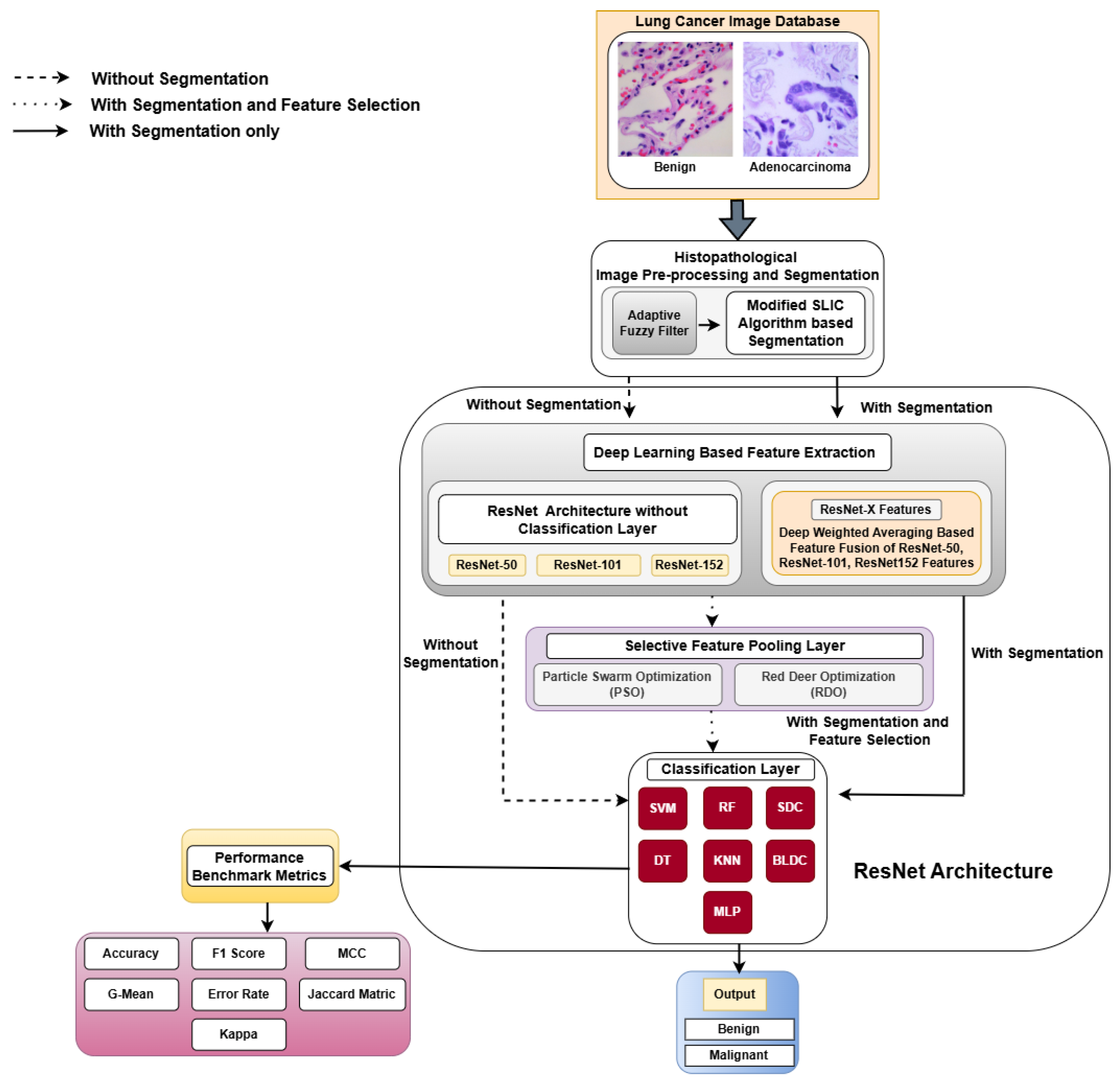
Figure 2.
a) Original ACA Image; b) Adaptive Fuzzy Filtered ACA Image; c) Original SLIC Superpixel Segmentation; d) Modified SLIC Superpixel Segmentation e) Modified SLIC Segmentation Result.
Figure 2.
a) Original ACA Image; b) Adaptive Fuzzy Filtered ACA Image; c) Original SLIC Superpixel Segmentation; d) Modified SLIC Superpixel Segmentation e) Modified SLIC Segmentation Result.
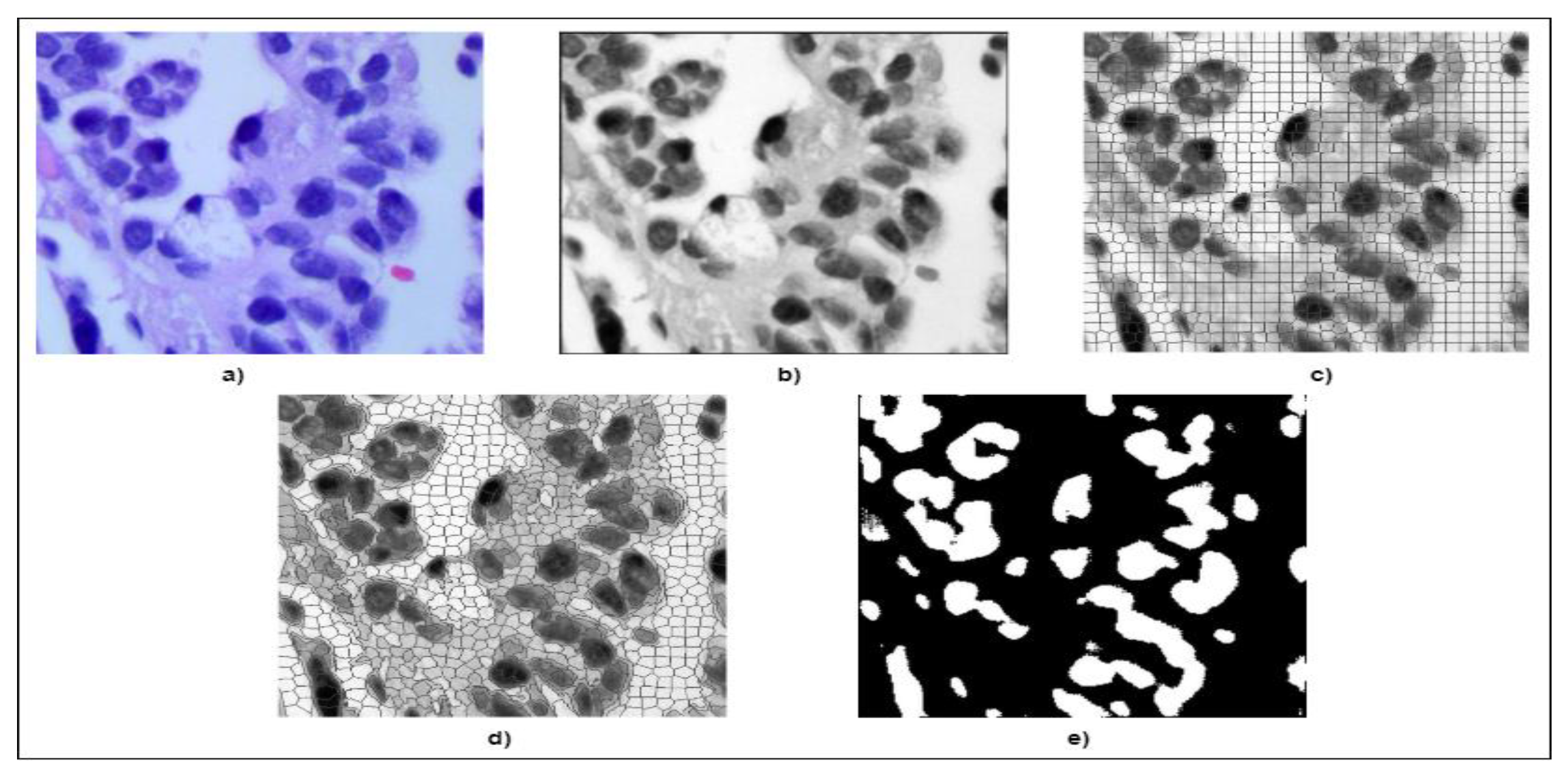
Figure 3.
Residual Mapping function.
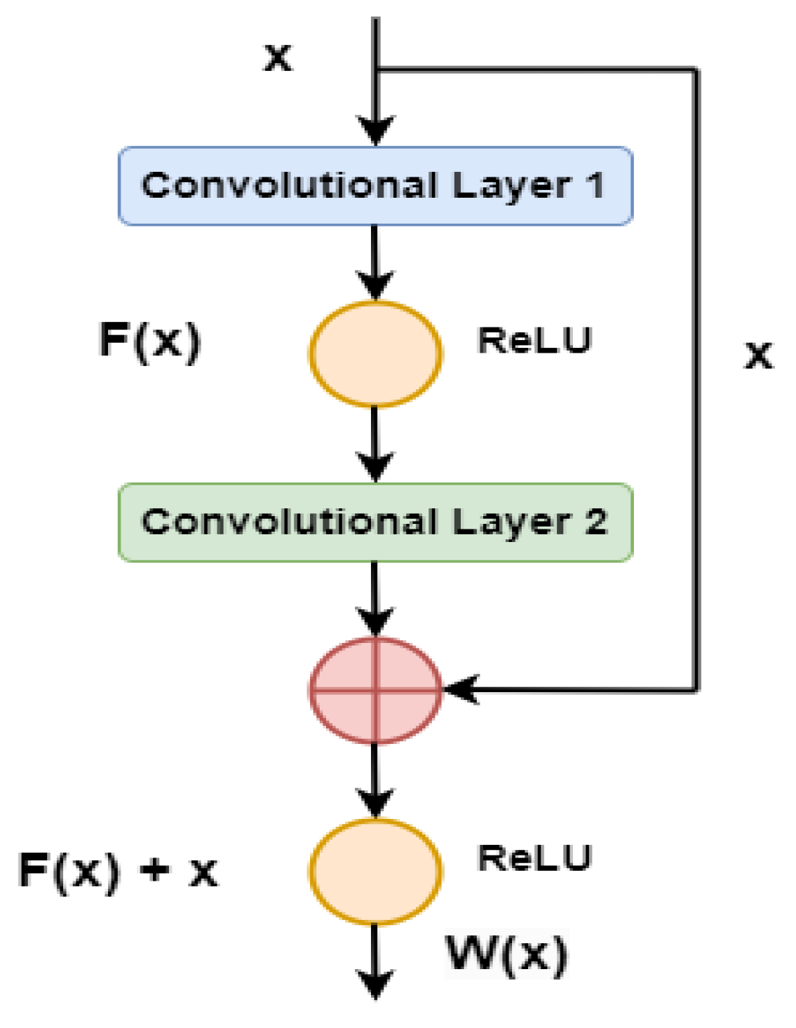
Figure 4.
Proposed ResNet Architecture.
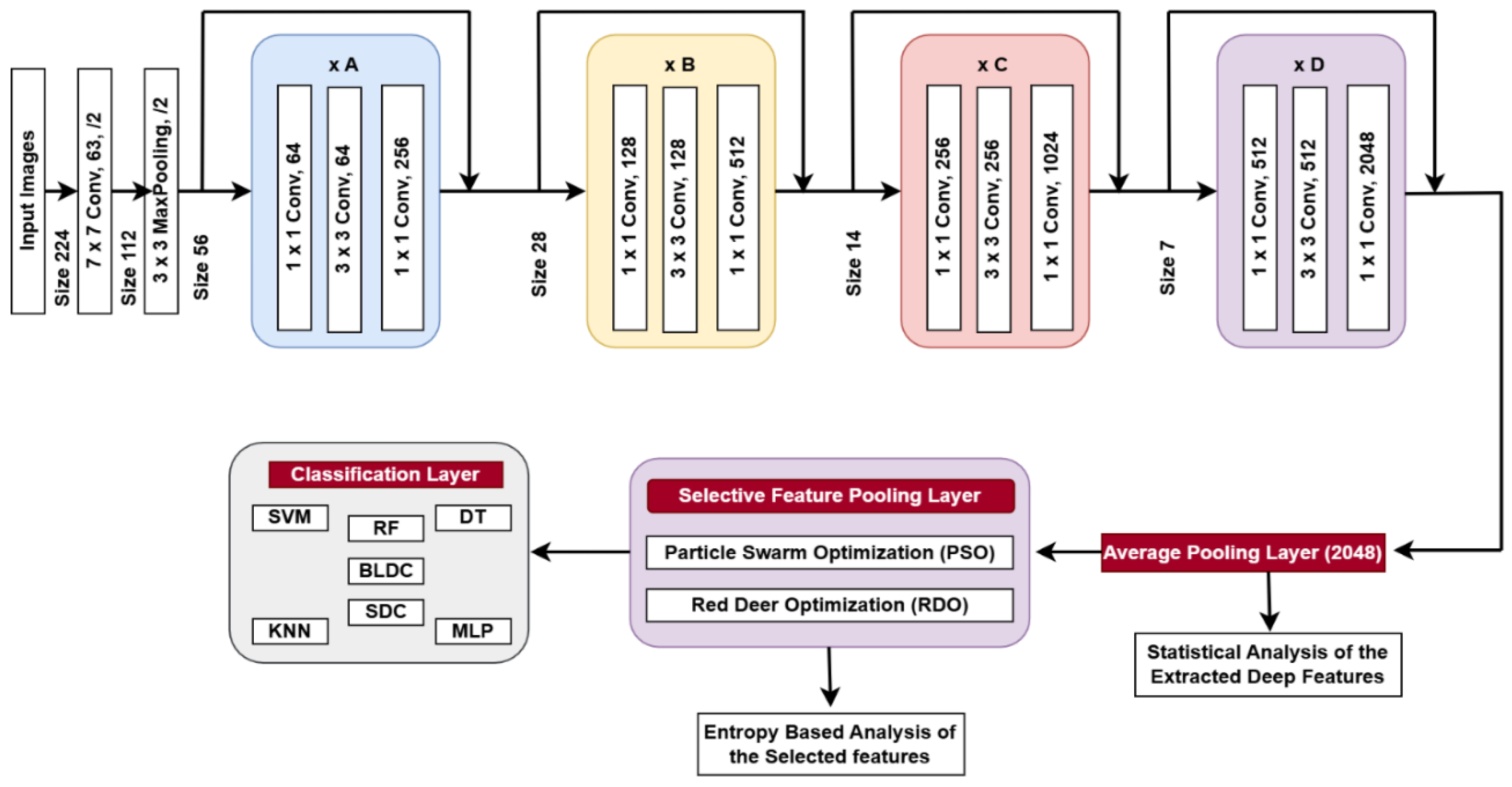
Figure 5.
Scatterplot matrix of ResNet-50, ResNet-101, ResNet-152 and ResNet-X for Cancerous and Non-Cancerous Data.
Figure 5.
Scatterplot matrix of ResNet-50, ResNet-101, ResNet-152 and ResNet-X for Cancerous and Non-Cancerous Data.
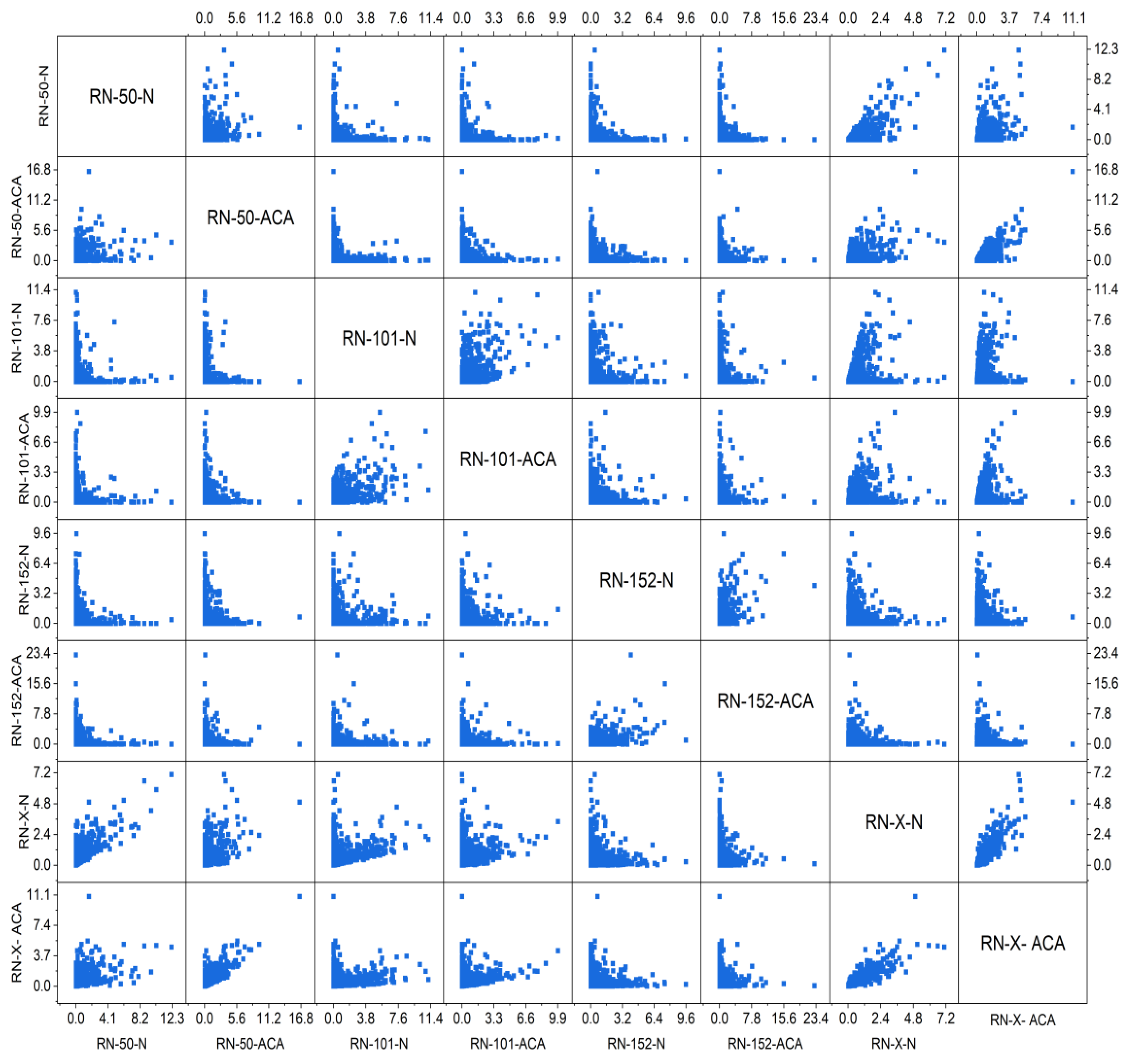
Figure 6.
Violin Plot of Class Distributions from Deep Features Extracted by ResNet Variants and DWAFF-RN-X Fused Features.
Figure 6.
Violin Plot of Class Distributions from Deep Features Extracted by ResNet Variants and DWAFF-RN-X Fused Features.
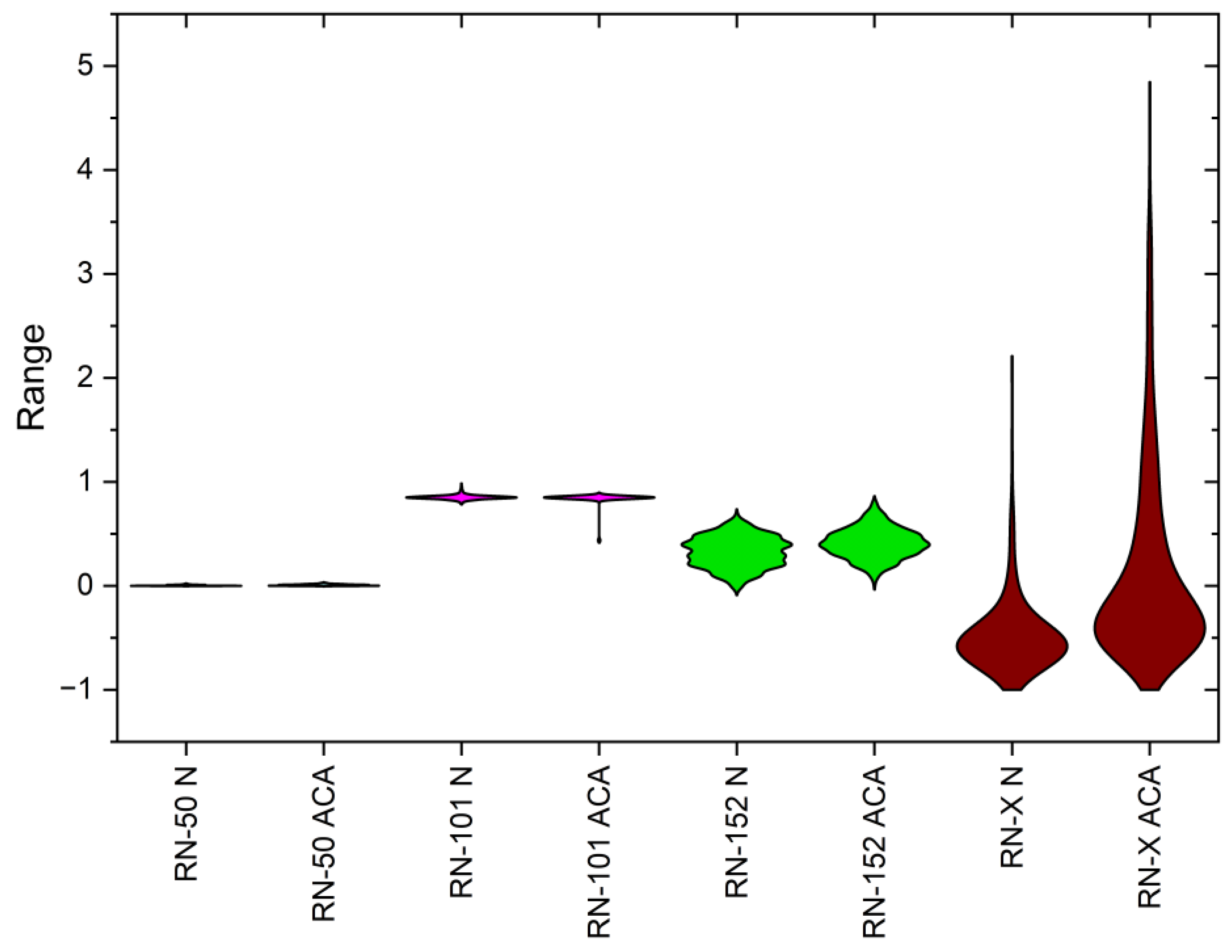
Figure 7.
Training vs Validation performance plot: With segmentation and PSO FS.
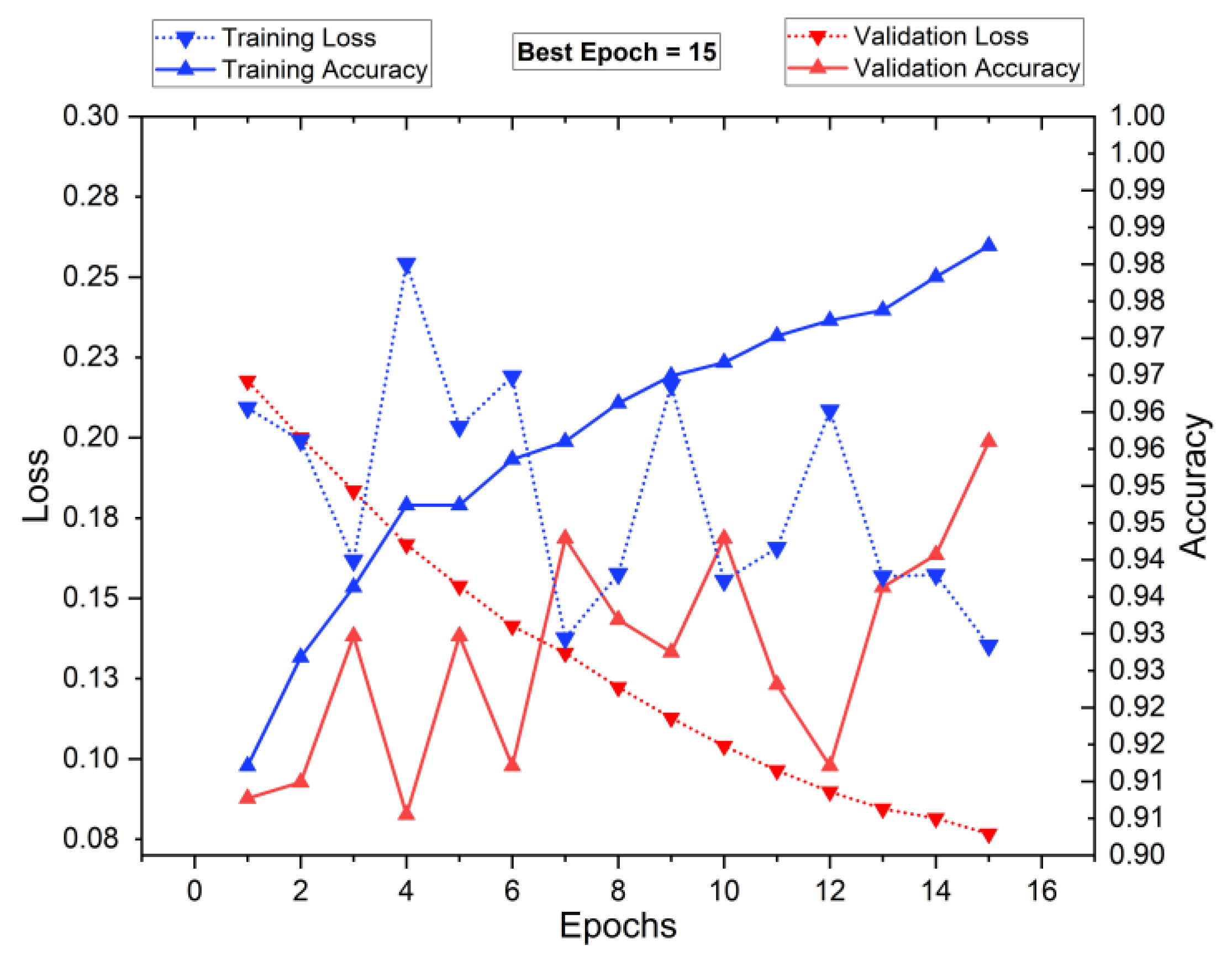
Figure 8.
Training vs Validation performance plot: With segmentation and RDO FS.
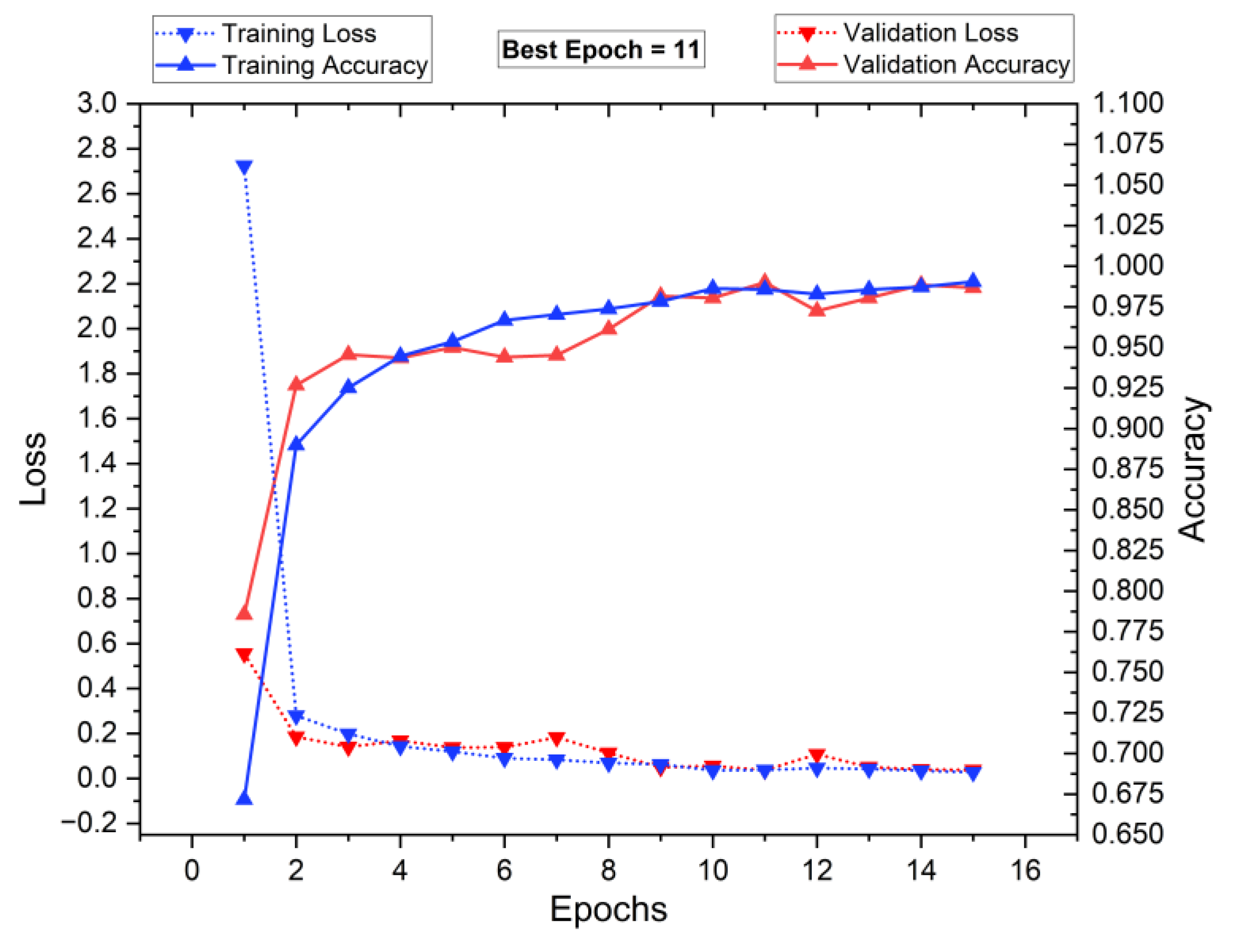
Figure 9.
Radar Plot for performance analysis of ResNet-50 and ResNet-101 with classifiers for K = 10.
Figure 9.
Radar Plot for performance analysis of ResNet-50 and ResNet-101 with classifiers for K = 10.
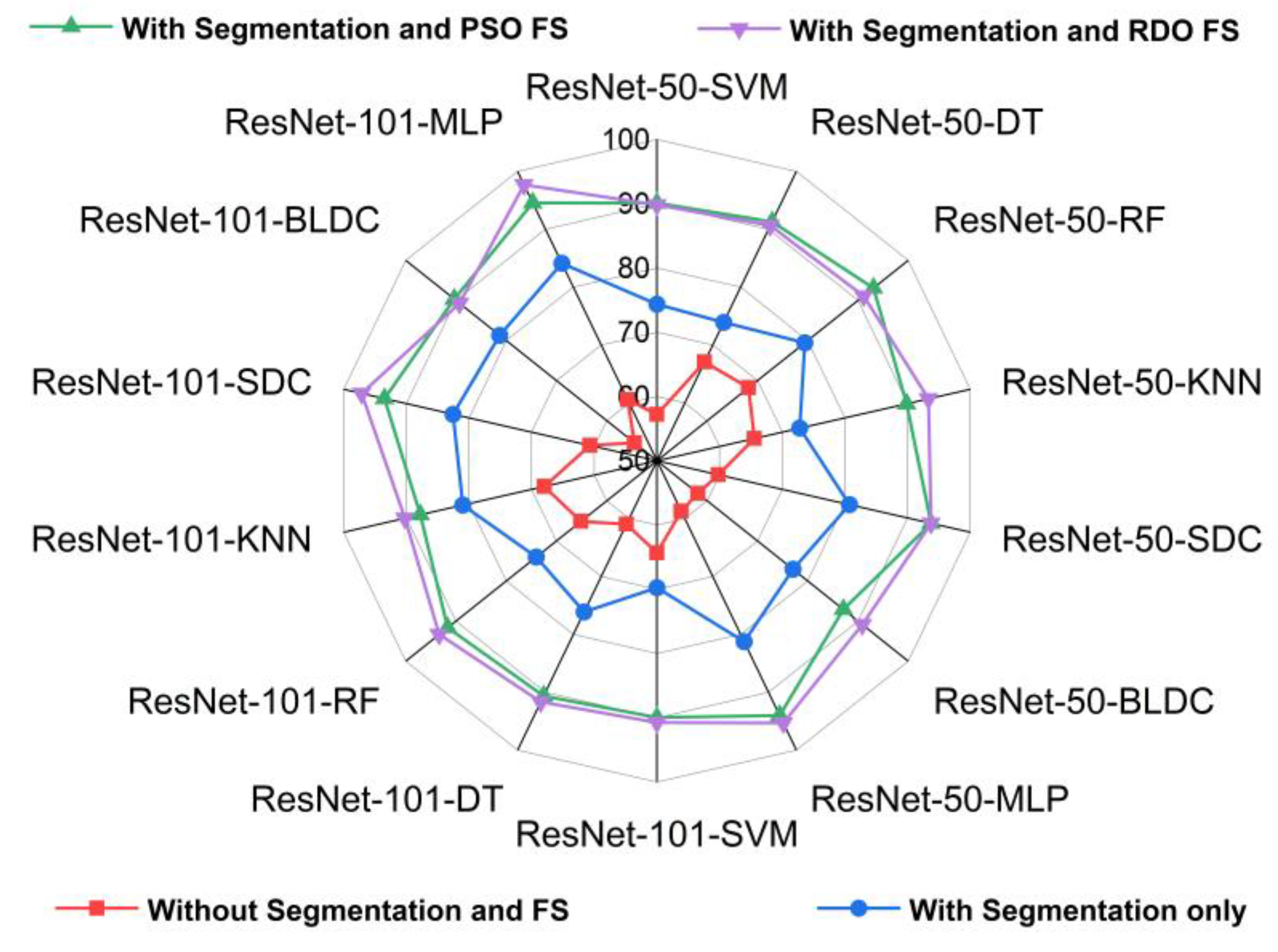
Figure 10.
Radar Plot for performance analysis of ResNet-152 and DWAFF based ResNet-X with classifiers for K = 10.
Figure 10.
Radar Plot for performance analysis of ResNet-152 and DWAFF based ResNet-X with classifiers for K = 10.
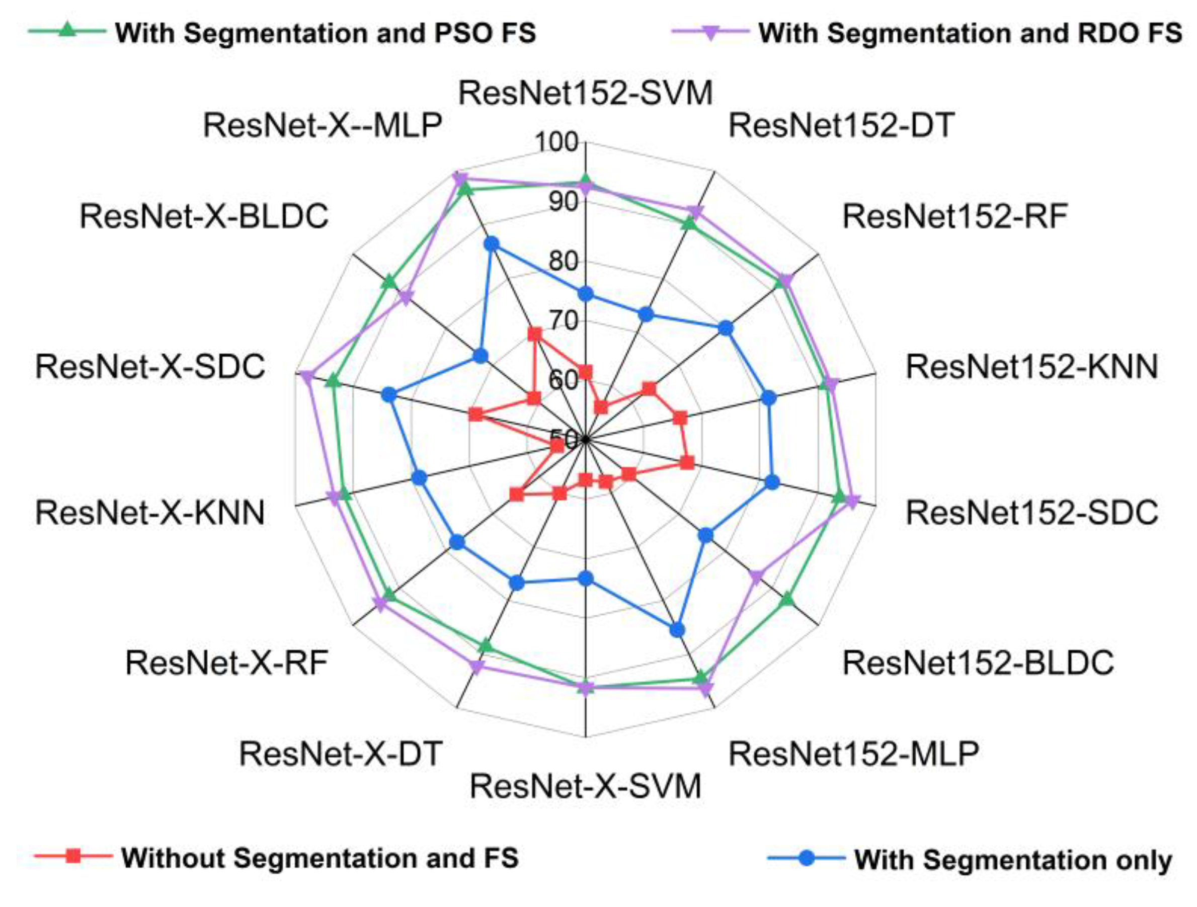
Figure 11.
Comparison of classifier performance using Jaccard Index vs F1 Score metrics for all the three cases when K = 10.
Figure 11.
Comparison of classifier performance using Jaccard Index vs F1 Score metrics for all the three cases when K = 10.
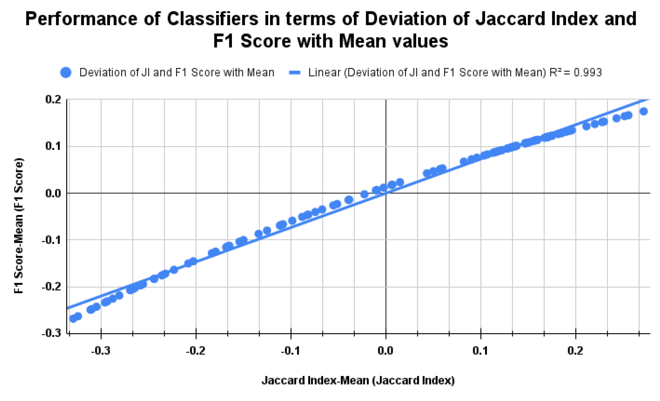
Table 1.
Residual Blocks of ResNet versions.
| ResNet Architectures | A | B | C | D |
|---|---|---|---|---|
| RN-50 | 3 | 4 | 6 | 3 |
| RN-101 | 3 | 4 | 23 | 3 |
| RN-152 | 3 | 8 | 36 | 3 |
Table 2.
Statistical Parameters of extracted deep features and fused features of Benign and Malignant data.
Table 2.
Statistical Parameters of extracted deep features and fused features of Benign and Malignant data.
| Statistical Parameters | ResNet-50 | ResNet-101 | ResNet-152 | DWAFF- ResNet-X | ||||
|---|---|---|---|---|---|---|---|---|
| N | ACA | N | ACA | N | ACA | N | ACA | |
| Mean | 0.33849 | 0.342961 | 0.344422 | 0.334716 | 0.350822 | 0.341976 | 0.453891 | 0.453709 |
| Variance | 0.714733 | 0.810025 | 0.792067 | 0.84634 | 0.798777 | 0.865552 | 0.380702 | 0.444597 |
| Skewness | 5.446134 | 5.940833 | 5.438773 | 6.000539 | 5.552535 | 6.224899 | 3.767961 | 4.486885 |
| Kurtosis | 43.68334 | 52.99684 | 42.83772 | 52.96116 | 46.38955 | 60.27778 | 21.14865 | 33.4781 |
| PCC | 0.499424 | 0.52724 | 0.495801 | 0.516755 | 0.494458 | 0.518542 | 0.938638 | 0.944338 |
| Dice Coefficient | 0.7512 | 0.7043 | 0.8028 | 0.7557 | 0.8598 | 0.8011 | 0.9038 | 0.8572 |
| CCA | 0.7018 | 0.7532 | 0.8293 | 0.8816 | ||||
Table 3.
Parameters of RDO.
| S No | Parameters | Value | S No | Parameters | Value |
|---|---|---|---|---|---|
| 1 | Number of Population | 100 | 6 | Beta | 0.5 |
| 2 | Simulation Time | 13 (s) | 7 | Gamma | 0.6 |
| 3 | Number of Male RD | 12 | 8 | Roar | 0.23 |
| 4 | Number of Hinds | 58 | 9 | Fight | 0.47 |
| 5 | Alpha | 0.9 | 10 | Mating | 0.78 |
Table 4.
Entropy based statistical Measures for PSO and RDO DR techniques.
| Statistical Measures | PSO | RDO | ||
|---|---|---|---|---|
| N | ACA | N | ACA | |
| Approximate Entropy | 1.2385 | 1.7816 | 2.0123 | 2.4893 |
| Shannon Entropy | 3.8523 | 4.9891 | 5.0821 | 5.8982 |
| Fuzzy Entropy | 0.4862 | 0.5231 | 0.7283 | 0.9182 |
Table 5.
Selection of Optimal Parameters for the Classifiers.
| Classifiers | Description |
|---|---|
| SVM | Kernel Function-RBF; Support vector coefficient, α = 1.8; Gaussian function bandwidth (σ) = 98; Bias term (b) = 0.012; Convergence Criterion-MSE. |
| KNN | K-5; Distance Metric-Euclidian; Weight-0.52; Criterion-MSE. |
| RF | Number of Trees-150; Maximum Depth-15; Bootstrap Sample Size-16; Class Weight-0.35. |
| DT | Maximum Depth-14; Impurity Criterion-MSE; Class Weight-0.25 |
| SDC | λ -0.458 along with the average target values for each class being 0.15 and 0.85 |
| MLP | Learning rate-0.45; Training Method-LM; Criterion-MSE. |
| BLDC | Mean and Covariance matrix , are calculated with a prior probability of 0.12; Convergence Criteria = MSE. |
Table 6.
Performance Metrics of the classifiers with their Significance.
| Performance Metrics | Equation | Significance |
|---|---|---|
| Accuracy (%) | The overall accuracy of the classifier's predictions. | |
| Error Rate (%) | The ratio of misclassified instances. | |
| F1 Score (%) | The harmonic mean of precision and recall, reflecting the classification accuracy for a specific class. | |
| MCC | The Pearson correlation between the observed and predicted classifications. |
|
| Jaccard Index (%) | The proportion of predicted true positives to the sum of predicted true positives and actual positives, regardless of their true or predicted status. | |
| g-mean (%) | A metric combines sensitivity and specificity into a singular value balancing both objectives. | |
| Kappa | Evaluates how well the observed and predicted classifications align, reflecting the consistency of the classification outcomes. |
Table 8.
Performance analysis of the classifiers when K = 10: Without Segmentation & With Segmentation.
Table 8.
Performance analysis of the classifiers when K = 10: Without Segmentation & With Segmentation.
| DL model with Classifiers | Without Segmentation and FS | With Segmentation only | ||||||||||||
|---|---|---|---|---|---|---|---|---|---|---|---|---|---|---|
| Accuracy (%) |
Error Rate (%) |
F1 Score (%) |
MCC | Kappa | Jaccard Index (%) |
G-Mean (%) |
Accuracy (%) |
Error Rate (%) |
F1 Score (%) |
MCC | Kappa | Jaccard Index (%) |
G-Mean (%) |
|
| ResNet-50-SVM | 57.200 | 42.800 | 57.808 | 0.144 | 0.144 | 40.655 | 57.182 | 74.350 | 25.650 | 77.690 | 0.510 | 0.487 | 63.519 | 72.827 |
| ResNet-50-DT | 67.060 | 32.940 | 68.339 | 0.342 | 0.341 | 51.905 | 66.938 | 73.910 | 26.090 | 68.676 | 0.507 | 0.478 | 52.295 | 71.996 |
| ResNet-50-RF | 68.230 | 31.770 | 70.813 | 0.370 | 0.365 | 54.814 | 67.654 | 79.420 | 20.580 | 79.788 | 0.589 | 0.588 | 66.373 | 79.399 |
| ResNet-50-KNN | 65.540 | 34.460 | 63.611 | 0.313 | 0.311 | 46.640 | 65.325 | 72.790 | 27.210 | 76.492 | 0.480 | 0.456 | 61.933 | 71.066 |
| ResNet-50-SDC | 59.790 | 40.210 | 56.393 | 0.198 | 0.196 | 39.269 | 59.280 | 80.730 | 19.270 | 78.859 | 0.625 | 0.615 | 65.097 | 80.243 |
| ResNet-50-BLDC | 58.150 | 41.850 | 56.247 | 0.164 | 0.163 | 39.127 | 57.987 | 77.090 | 22.910 | 75.289 | 0.548 | 0.542 | 60.370 | 76.745 |
| ResNet-50-MLP | 58.700 | 41.300 | 59.310 | 0.174 | 0.174 | 42.157 | 58.681 | 81.250 | 18.750 | 82.353 | 0.630 | 0.625 | 70.000 | 81.009 |
| ResNet-101-SVM | 64.330 | 35.670 | 61.740 | 0.289 | 0.287 | 44.655 | 63.973 | 69.760 | 30.240 | 66.623 | 0.402 | 0.395 | 49.950 | 69.124 |
| ResNet-101-DT | 60.940 | 39.060 | 60.940 | 0.219 | 0.219 | 43.823 | 60.940 | 76.110 | 23.890 | 74.359 | 0.527 | 0.522 | 59.183 | 75.803 |
| ResNet-101-RF | 65.130 | 34.870 | 66.156 | 0.303 | 0.303 | 49.427 | 65.060 | 74.020 | 25.980 | 74.272 | 0.481 | 0.480 | 59.074 | 74.014 |
| ResNet-101-KNN | 67.969 | 32.031 | 69.630 | 0.362 | 0.359 | 53.409 | 67.748 | 80.980 | 19.020 | 80.930 | 0.620 | 0.620 | 67.969 | 80.980 |
| ResNet-101-SDC | 60.680 | 39.320 | 60.719 | 0.214 | 0.214 | 43.595 | 60.680 | 82.550 | 17.450 | 81.791 | 0.653 | 0.651 | 69.191 | 82.445 |
| ResNet-101-BLDC | 54.450 | 45.550 | 54.345 | 0.089 | 0.089 | 37.311 | 54.450 | 81.310 | 18.690 | 82.983 | 0.639 | 0.626 | 70.915 | 80.714 |
| ResNet-101-MLP | 60.530 | 39.470 | 60.605 | 0.211 | 0.211 | 43.477 | 60.530 | 84.120 | 15.880 | 81.797 | 0.706 | 0.682 | 69.201 | 83.147 |
| ResNet152-SVM | 61.360 | 38.640 | 64.790 | 0.232 | 0.227 | 47.918 | 60.582 | 74.480 | 25.520 | 72.470 | 0.495 | 0.490 | 56.826 | 74.121 |
| ResNet152-DT | 55.970 | 44.030 | 58.055 | 0.120 | 0.119 | 40.899 | 55.749 | 73.370 | 26.630 | 76.585 | 0.486 | 0.467 | 62.055 | 72.074 |
| ResNet152-RF | 63.670 | 36.330 | 62.849 | 0.274 | 0.273 | 45.825 | 63.632 | 80.070 | 19.930 | 78.563 | 0.607 | 0.601 | 64.694 | 79.761 |
| ResNet152-KNN | 66.270 | 33.730 | 69.914 | 0.335 | 0.325 | 53.744 | 65.154 | 81.510 | 18.490 | 83.525 | 0.650 | 0.630 | 71.711 | 80.587 |
| ResNet152-SDC | 67.550 | 32.450 | 61.465 | 0.370 | 0.351 | 44.368 | 65.679 | 82.090 | 17.910 | 79.728 | 0.660 | 0.642 | 66.290 | 81.259 |
| ResNet152-BLDC | 59.340 | 40.660 | 60.432 | 0.187 | 0.187 | 43.299 | 59.276 | 75.770 | 24.230 | 69.889 | 0.560 | 0.515 | 53.715 | 73.210 |
| ResNet152-MLP | 57.880 | 42.120 | 58.633 | 0.158 | 0.158 | 41.476 | 57.851 | 85.420 | 14.580 | 85.420 | 0.708 | 0.708 | 74.551 | 85.420 |
| ResNet-X-SVM | 56.780 | 43.220 | 56.892 | 0.136 | 0.136 | 39.755 | 56.779 | 73.300 | 26.700 | 71.160 | 0.471 | 0.466 | 55.231 | 72.924 |
| ResNet-X-DT | 60.020 | 39.980 | 61.617 | 0.201 | 0.200 | 44.526 | 59.876 | 76.690 | 23.310 | 76.100 | 0.535 | 0.534 | 61.420 | 76.650 |
| ResNet-X-RF | 64.800 | 35.200 | 63.942 | 0.296 | 0.296 | 46.996 | 64.756 | 77.580 | 22.420 | 74.523 | 0.568 | 0.552 | 59.391 | 76.646 |
| ResNet-X-KNN | 54.850 | 45.150 | 54.864 | 0.097 | 0.097 | 37.801 | 54.850 | 78.650 | 21.350 | 81.862 | 0.613 | 0.573 | 69.294 | 76.630 |
| ResNet-X-SDC | 68.930 | 31.070 | 69.756 | 0.379 | 0.379 | 53.558 | 68.876 | 83.850 | 16.150 | 82.916 | 0.681 | 0.677 | 70.817 | 83.671 |
| ResNet-X-BLDC | 61.060 | 38.940 | 62.851 | 0.222 | 0.221 | 45.826 | 60.870 | 72.550 | 27.450 | 77.154 | 0.493 | 0.451 | 62.805 | 69.696 |
| ResNet-X--MLP | 69.610 | 30.390 | 73.185 | 0.407 | 0.392 | 57.709 | 68.322 | 86.460 | 13.540 | 86.318 | 0.729 | 0.729 | 75.929 | 86.454 |
Table 9.
Performance analysis of the classifiers when K = 10: With Segmentation and Feature Selection (FS).
Table 9.
Performance analysis of the classifiers when K = 10: With Segmentation and Feature Selection (FS).
| DL model with Classifiers | With Segmentation and PSO FS | With Segmentation and RDO FS | ||||||||||||
|---|---|---|---|---|---|---|---|---|---|---|---|---|---|---|
| Accuracy (%) |
Error Rate (%) |
F1 Score (%) |
MCC | Kappa | Jaccard Index (%) |
G-Mean (%) |
Accuracy (%) |
Error Rate (%) |
F1 Score (%) |
MCC | Kappa | Jaccard Index (%) |
G-Mean (%) |
|
| ResNet-50-SVM | 90.110 | 9.890 | 90.111 | 0.802 | 0.802 | 82.002 | 90.110 | 89.840 | 10.160 | 89.253 | 0.802 | 0.797 | 80.592 | 89.674 |
| ResNet-50-DT | 91.290 | 8.710 | 91.301 | 0.826 | 0.826 | 83.995 | 91.290 | 90.630 | 9.370 | 90.061 | 0.818 | 0.813 | 81.918 | 90.449 |
| ResNet-50-RF | 93.110 | 6.890 | 93.225 | 0.863 | 0.862 | 87.309 | 93.095 | 91.140 | 8.860 | 90.904 | 0.824 | 0.823 | 83.324 | 91.103 |
| ResNet-50-KNN | 89.840 | 10.160 | 89.814 | 0.797 | 0.797 | 81.511 | 89.840 | 93.350 | 6.650 | 93.218 | 0.868 | 0.867 | 87.297 | 93.330 |
| ResNet-50-SDC | 93.750 | 6.250 | 94.060 | 0.880 | 0.875 | 88.785 | 93.605 | 93.750 | 6.250 | 94.000 | 0.878 | 0.875 | 88.680 | 93.657 |
| ResNet-50-BLDC | 87.100 | 12.900 | 86.484 | 0.745 | 0.742 | 76.186 | 86.981 | 90.880 | 9.120 | 91.043 | 0.818 | 0.818 | 83.559 | 90.862 |
| ResNet-50-MLP | 94.010 | 5.990 | 93.833 | 0.882 | 0.880 | 88.383 | 93.966 | 95.310 | 4.690 | 95.475 | 0.909 | 0.906 | 91.342 | 95.240 |
| ResNet-101-SVM | 89.960 | 10.040 | 89.895 | 0.799 | 0.799 | 81.645 | 89.958 | 90.760 | 9.240 | 89.935 | 0.826 | 0.815 | 81.710 | 90.389 |
| ResNet-101-DT | 90.620 | 9.380 | 90.717 | 0.813 | 0.812 | 83.010 | 90.614 | 91.670 | 8.330 | 92.083 | 0.838 | 0.833 | 85.327 | 91.522 |
| ResNet-101-RF | 91.670 | 8.330 | 91.015 | 0.842 | 0.833 | 83.512 | 91.380 | 93.350 | 6.650 | 93.218 | 0.868 | 0.867 | 87.297 | 93.330 |
| ResNet-101-KNN | 87.760 | 12.240 | 87.917 | 0.756 | 0.755 | 78.439 | 87.750 | 90.230 | 9.770 | 90.318 | 0.805 | 0.805 | 82.346 | 90.225 |
| ResNet-101-SDC | 93.490 | 6.510 | 93.188 | 0.873 | 0.870 | 87.245 | 93.385 | 97.130 | 2.870 | 97.182 | 0.943 | 0.943 | 94.518 | 97.113 |
| ResNet-101-BLDC | 90.360 | 9.640 | 90.385 | 0.807 | 0.807 | 82.457 | 90.360 | 89.320 | 10.680 | 89.457 | 0.787 | 0.786 | 80.925 | 89.311 |
| ResNet-101-MLP | 94.530 | 5.470 | 94.628 | 0.891 | 0.891 | 89.804 | 94.512 | 97.660 | 2.340 | 97.629 | 0.954 | 0.953 | 95.368 | 97.651 |
| ResNet152-SVM | 93.220 | 6.780 | 93.113 | 0.865 | 0.864 | 87.113 | 93.207 | 92.370 | 7.630 | 92.443 | 0.848 | 0.847 | 85.948 | 92.365 |
| ResNet152-DT | 90.110 | 9.890 | 90.737 | 0.810 | 0.802 | 83.045 | 89.855 | 92.570 | 7.430 | 92.482 | 0.852 | 0.851 | 86.015 | 92.563 |
| ResNet152-RF | 92.180 | 7.820 | 91.885 | 0.846 | 0.844 | 84.988 | 92.108 | 93.030 | 6.970 | 92.591 | 0.867 | 0.861 | 86.204 | 92.841 |
| ResNet152-KNN | 91.460 | 8.540 | 91.203 | 0.831 | 0.829 | 83.829 | 91.413 | 92.310 | 7.690 | 92.533 | 0.848 | 0.846 | 86.104 | 92.262 |
| ResNet152-SDC | 93.750 | 6.250 | 93.478 | 0.878 | 0.875 | 87.755 | 93.657 | 95.960 | 4.040 | 95.954 | 0.919 | 0.919 | 92.223 | 95.960 |
| ResNet152-BLDC | 93.230 | 6.770 | 93.011 | 0.866 | 0.865 | 86.936 | 93.177 | 86.710 | 13.290 | 85.863 | 0.740 | 0.734 | 75.228 | 86.503 |
| ResNet152-MLP | 94.520 | 5.480 | 94.477 | 0.891 | 0.890 | 89.532 | 94.517 | 96.350 | 3.650 | 96.369 | 0.927 | 0.927 | 92.993 | 96.349 |
| ResNet-X-SVM | 91.670 | 8.330 | 91.212 | 0.838 | 0.833 | 83.844 | 91.522 | 91.640 | 8.360 | 91.850 | 0.834 | 0.833 | 84.929 | 91.604 |
| ResNet-X-DT | 88.600 | 11.400 | 88.426 | 0.772 | 0.772 | 79.254 | 88.587 | 92.180 | 7.820 | 91.928 | 0.845 | 0.844 | 85.062 | 92.127 |
| ResNet-X-RF | 92.190 | 7.810 | 91.850 | 0.847 | 0.844 | 84.929 | 92.096 | 94.010 | 5.990 | 94.293 | 0.885 | 0.880 | 89.201 | 93.880 |
| ResNet-X-KNN | 91.660 | 8.340 | 91.830 | 0.834 | 0.833 | 84.894 | 91.636 | 93.220 | 6.780 | 93.425 | 0.866 | 0.864 | 87.662 | 93.168 |
| ResNet-X-SDC | 93.490 | 6.510 | 93.113 | 0.875 | 0.870 | 87.114 | 93.330 | 97.860 | 2.140 | 97.836 | 0.957 | 0.957 | 95.764 | 97.854 |
| ResNet-X-BLDC | 92.180 | 7.820 | 92.300 | 0.844 | 0.844 | 85.701 | 92.167 | 88.540 | 11.460 | 88.774 | 0.772 | 0.771 | 79.813 | 88.516 |
| ResNet-X--MLP | 96.490 | 3.510 | 96.476 | 0.930 | 0.930 | 93.192 | 96.489 | 98.680 | 1.320 | 98.670 | 0.974 | 0.974 | 97.375 | 98.677 |
Table 10.
Comparison of Classifier Performance with different datasets.
| S No | Authors | Dataset Used | Classification Models | Accuracy (%) |
|---|---|---|---|---|
| 1 | Jain DK et al., (2022) [41] | 1500 images from LZ2500 dataset | Kernel PCA combined with Faster Deep Belief Networks | 97.10% |
| 2 | Civit-Masot J et al., (2022) [42] | 15,000 images from LC25000 dataset | Custom Architecture with 3 Convolution and 2 dense layers | 99.69% with 50 epochs |
| 3 | Iftikhar Naseer et al., (2023) [43] | LUNA 16 Database |
LungNet-SVM | 97.64% |
| 4 | Wang et al., (2023) [44] | 993 WSIs from TCGA dataset | A novel multiplex-detection-based MIL model | 90.52% |
| 5 | Mehedi Masud et al., (2021) [45] | LC25000 dataset | Custom CNN architecture consisting of 3 Convolution and 1 FC layers | 96.33% |
| 6 | Radical Rakhman Wahid et al., (2023) [46] |
LC25000 Database | Customized CNN Model | 93.02% |
| 7 | Mingyang Liu et al., (2023) [47] | First Hospital of Jilin University - Dataset | MLP IN MLP | 95.31% |
| 8 | Gupta S et al., (2022) [48] | TCGA dataset | Deep CNN | 92% |
| 9 | Liu Y et al., (2022) [49] | 766 lung WSIs from First Hospital of Baiqiu’en and LC25000 dataset | SE-ResNet-50 with novel activation function CroRELU | 98.33% |
| 10 | Wang X et al., (2023) [50] | 988 samples with both CNV and histological data | LungDIG: Combination of InceptionV3 with MLP | 87.10% |
| 11 | Rekka, Mastouri. et al., (2021) [51] | LUNA16 Database (3186 CT images) |
BCNN [VGG16, VGG19] | 91.99% |
| 12 | Phankokkruad, M (2021) [52] | LC25000 Database | Ensemble ResNet50V2 |
91% 90% |
| 13 | Bukhari, S. et al., (2020) [53] | CRAG Dataset | ResNet-50 | 93.91% |
| 14 | Karthikeyan Shanmugam, Harikumar Rajaguru This Research |
LC25000 Database |
Feature Extraction – RDO TL model – EfficientNetB0 with MLP classifier |
98.698% |
Table 11.
Computational Complexity of the classifiers.
| Deep Feature Extraction |
Classifiers | Without Segmentation | With Segmentation | With Segmentation and PSO Feature Selection | With Segmentation and RDO Feature Selection |
|---|---|---|---|---|---|
| ResNet-50 | SVM | ||||
| DT | |||||
| RF | |||||
| KNN | |||||
| SDC | |||||
| BLDC | |||||
| MLP | |||||
| ResNet-101 | SVM | ||||
| DT | |||||
| RF | |||||
| KNN | |||||
| SDC | |||||
| BLDC | |||||
| MLP | |||||
| ResNet-152 | SVM | ||||
| DT | |||||
| RF | |||||
| KNN | |||||
| SDC | |||||
| BLDC | |||||
| MLP | |||||
| DWAFF - ResNet-X |
SVM | ||||
| DT | |||||
| RF | |||||
| KNN | |||||
| SDC | |||||
| BLDC | |||||
| MLP |
Disclaimer/Publisher’s Note: The statements, opinions and data contained in all publications are solely those of the individual author(s) and contributor(s) and not of MDPI and/or the editor(s). MDPI and/or the editor(s) disclaim responsibility for any injury to people or property resulting from any ideas, methods, instructions or products referred to in the content. |
© 2025 by the authors. Licensee MDPI, Basel, Switzerland. This article is an open access article distributed under the terms and conditions of the Creative Commons Attribution (CC BY) license (http://creativecommons.org/licenses/by/4.0/).
Copyright: This open access article is published under a Creative Commons CC BY 4.0 license, which permit the free download, distribution, and reuse, provided that the author and preprint are cited in any reuse.