Submitted:
07 February 2025
Posted:
10 February 2025
Read the latest preprint version here
Abstract
Baseflow, the portion of streamflow sustained by groundwater discharge, is crucial for maintaining river ecosystems. Irrigation practices significantly influence this interaction, with varying impacts depending on the method and intensity of water use. Excessive groundwater extraction can deplete aquifers, reduce baseflow, and disrupt the balance between groundwater and surface water. This study evaluates the effects of irrigation expansion on baseflows and develops a predictive tool to assess future agricultural impacts on water resources. The SWAT+gwflow model is applied to the San Antonio Catchment, Uruguay, a region dominated by intensive horticulture and citrus farming, where irrigation relies on groundwater pumping. With increasing irrigation demands, the study finds a decline in both baseflow and groundwater levels due to higher extraction rates. This modeling approach enables the identification of spatial variations in baseflow, surface water–groundwater exchanges, and groundwater storage, providing valuable insights at a sub-catchment scale. The findings contribute to a better understanding of hydrological responses to irrigation expansion, supporting sustainable water management strategies in agricultural regions.
Keywords:
SWAT+gwflow
; surface water – groundwater interactions
; irrigation expansion
1. Introduction
In hydrology, baseflow refers to the portion of streamflow that originates from groundwater seepage into a river or stream [1]. It represents the sustained flow of water in a stream during periods without significant rainfall or snowmelt, serving as the primary source of streamflow during dry weather. Understanding the interactions between baseflow, groundwater, and irrigation is crucial for effective water resource management [2]. These interactions are especially significant in catchments where groundwater is the primary source for irrigation. Excessive extraction of groundwater can deplete aquifers, diminish baseflows, and disrupt the delicate balance between groundwater and baseflow. Ensuring sustainable water use and maintaining long-term water availability requires quantifying these interactions effectively.
Irrigation practices play a critical role in shaping these interactions, with different types of irrigation having varying impacts on water resources [3]. Surface water irrigation, which relies on rivers, lakes, or reservoirs, can alter streamflow dynamics by modifying natural flow regimes, potentially reducing environmental flows needed to sustain aquatic ecosystems [4]. Additionally, to add complexity, some exceptions to these patterns have been identified, where excess irrigation can, in certain cases, contribute to increased baseflows [5]. In contrast, groundwater irrigation depends on aquifer withdrawals, which can lower water tables when extraction rates exceed natural recharge [6]. These impacts are complex to evaluate, as they depend on factors such as recharge rates, soil properties, climate conditions, and irrigation efficiency. For this reason, coupled models that integrate surface water and groundwater dynamics provide a valuable tool for assessing these interactions, allowing for more accurate predictions of water availability and the effects of different irrigation strategies on hydrological processes [7].
The SWAT+gwflow model represents a significant advancement in hydrological modelling. By coupling a physically based, spatially distributed groundwater flow module [8] with the SWAT+ model [9], this tool is designed to simulate the complex exchanges between groundwater - surface water (GW-SW) more effectively. The combined model takes advantage of the widely used SWAT+ to represent surface hydrological processes and agricultural practices [10,11,12,13,14], while adding a two-dimensional approach to simulate groundwater fluxes. The SWAT+gwflow model has demonstrated improved performance in representing baseflows compared to the standalone SWAT+ [15,16,17,18]. This makes it a valuable tool for assessing the impacts of irrigation expansion.
The San Antonio catchment, characterized by intensive horticultural and citrus crops irrigated by pumping wells, serves as an ideal experimental area for the characterization of GW-SW [19,20]. This catchment is particularly relevant due to its dependence on groundwater resources and the availability of a relatively rich hydrometeorological network. Furthermore, the area has potential for further irrigation expansion, which could significantly affect water availability and the balance between groundwater and surface water [20]. Such an expansion would increase the demand for groundwater resources and potentially alter baseflows, requiring careful evaluation to ensure sustainable water management. In this context, the objective of this work is to evaluate the impacts of irrigation expansion on baseflows and to develop a predictive tool for assessing the effects of future agricultural practices on surface and groundwater resources, ensuring sustainable water management in groundwater-dependent catchments.
2. Materials and Methods
2.1. Study area and dataset
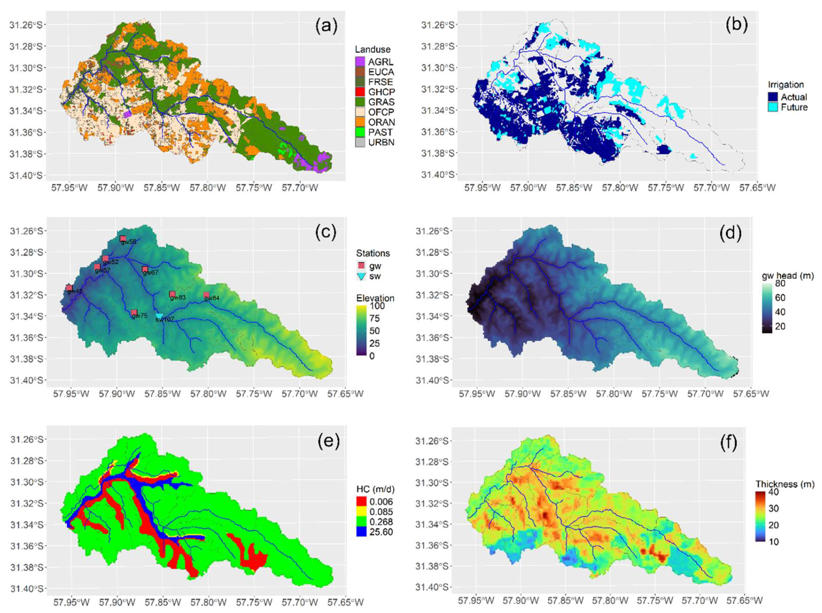
The San Antonio Catchment, covering an area of 225 km², is in north-western Uruguay and experiences a humid subtropical climate, as classified by the Köppen climate system [21]. The mean annual rainfall is 1,430 mm, with lower monthly precipitation during the winter months (June, July, and August). Average daily temperatures range from 10 to 15 °C in winter and from 20 to 30 °C in summer [19]. The monitoring network, maintained by the “Departamento del Agua - CENUR Litoral Norte” since 2018, consists of 8 observation wells for groundwater, 1 hydrometric station with reliable discharge computations for surface water (Figure 1c), and 14 rain gauges distributed throughout the region.
The land use within the catchment (Figure 1a) is characterized by a significant proportion of open field horticulture (OFCP, 34.7%) and citriculture (ORAN, 20.3%), both of which rely on a combination of rainfed crops and supplemental irrigation, depending on the practices and resources available to each farmer [22]. Most of the irrigation zones are in the southwest of the basin, while the northern area holds potential for developing supplementary irrigation, particularly for citrus crops (Figure 1b). In addition, the catchment features a large proportion of grassland (GRAS, 35.6%) and pastures (PAST, 0.6%), both utilised for grazing livestock. Other minor land uses include forestry plantations (EUCA, 1.6%), native forest (FRSE, 4.2%), greenhouse horticulture (GHCP, 0.8%), summer crops (AGRL, 2.1%), and urban areas (URBN, 0.1%). This diverse land use pattern reflects the multifunctional nature of the catchment.
The terrain is relatively flat, characterized by a rolling landscape with occasional small hills (Figure 1c). The soils are predominantly Argiudolls and Hapluderts, with textures ranging from silty clay to silty clay loam [23]. Geology comprises sedimentary deposits and fissured basalt rocks from the Cretaceous-Tertiary periods, which form part of the Salto-Arapey aquifer [24,25]. The Global Permeability (GLHYMPS) dataset [26] identifies four zones with distinctive aquifer hydraulic conductivities (Figure 1e). Additionally, SoilGrids data [27] indicates an absolute depth to bedrock (aquifer thickness) ranging from 10 to 40 meters (Figure 1f).
2.2. Groundwater – Surface water model
SWAT+gwflow [8] is an extension of the SWAT+ model [9] that integrates a computationally efficient, 2D finite-difference groundwater flow model to enhance the simulation of GW-SW. This extension provides a more explicit representation of groundwater flow dynamics. In the model, surface water processes are represented through Hydrologic Response Units (HRUs), which are polygons defined by the combination of land use, soil type, and slope. HRUs serve as the primary elements for hydrological production functions, such as infiltration, exfiltration, and surface runoff. Their structure remains consistent with the standalone SWAT+ model. The model's transfer function—governing surface and subsurface routing as well as storage—is defined by channels and an aquifer grid. Each aquifer grid cell is linked to its corresponding HRUs polygons. This feature allows for the representation of spatial variability in aquifer recharge (derived from SWAT+) and aquifer outflows (e.g. groundwater pumping or discharge to channels).
The San Antonio catchment is modelled with 411 HRUs, ranging in size from 0.1 to 2,200 hectares; 37 channels, varying in length from 70 to 9,000 meters; 24 subbasins, spanning from 0.22 to 31 km²; and an aquifer grid comprising 161 by 284 cells, each with a resolution of 100 by 100 meters. Precipitation data from local rain gauges were pre-processed using inverse distance interpolation to calculate the average precipitation for each sub-catchment, ensuring accurate spatial distribution of rainfall inputs. Agricultural management practices, including crop types, planting and harvesting schedules, fertilization, and irrigation strategies, were identified through interviews with local farmers. This information was then incorporated into the model to reflect the dominant land uses across the catchment. Irrigation pumping rates were set based on the water demands of irrigated crops, ensuring that simulated water usage aligns with real-world agricultural requirements. Key aquifer properties, such as aquifer thickness and hydraulic conductivity, were defined using global datasets (Figure 1e and Figure 1f). Boundary conditions were assumed to have constant hydraulic heads, enabling groundwater exchange with adjacent catchments.
The model was optimized during the period from 1 February 2019 to 1 August 2021. Results were verified for the periods from 8 August 2018 to 1 February 2019 and 1 September 2021 to 5 February 2021. These optimization and verification windows were selected to ensure the occurrence of dry and wet periods, with the optimization window comprising two-thirds of the total period of available data. For that purpose, a two-phase supervised random optimization process is used. This process involves a series of iterations, beginning with a uniform distribution across specified parameter ranges. In each iteration, the model runs 360 times, and each simulation is evaluated using the objective function specific to the corresponding optimization phase. The first phase prioritized achieving the best possible fit for streamflow simulations, assessed using the Kling-Gupta Efficiency (KGE) metric [28]. The model parameters optimized during this phase are listed in Table 1.
The second phase aimed to minimize the normalized root mean square error (nRMSE) for groundwater heads and surface baseflow, further improving the model’s accuracy in simulating subsurface hydrological processes and baseflow dynamics. Baseflow separation is made by Lyne-Hollick filter [29] with the R package grwat [30]. The parameters adjusted during this phase are detailed in Table 2. Instead of using a partitioned period of the time series, six observation wells were used for optimization (gw46, gw56, gw57, gw67, gw75, gw84) and two for verification (gw52, gw83). This approach was chosen to address gaps in the records at certain sites.
2.3. Assumptions for water pumping in irrigation and irrigation expansion
Determining the amount of water extracted from groundwater in Uruguay is a challenging task, as the locations of all pumping wells are not well known, and the volume of water drawn from the aquifer by each well remains unknown. To address this issue, land use involving irrigated crops was identified through a field campaign and by referencing declared irrigation wells in the national database. Pumping wells used for other purposes, such as domestic and livestock water supply, were not considered, as the volume of water used for these purposes is assumed to be negligible compared to irrigation water in the catchment. Once the irrigated crops were identified, it was important to determine the amount of water extracted for irrigation. This volume could be estimated based on crop water requirements; however, in practice, farmers often lack formal irrigation guidelines. Instead, they rely on empirical knowledge and expert judgement regarding crop needs. As a result, irrigation may sometimes be applied in excess or deficit. For this reason, the water stress threshold that triggers irrigation in the model was optimized (table 2). At this stage, citrus, greenhouse horticulture, and open-field horticulture were modelled with three different water stress thresholds, each representing the average condition for its respective crop type.
The effect of irrigation expansion on baseflow is estimated using the SWAT+gwflow model. To this end, it is assumed that irrigation expansion will occur only in areas currently dedicated to rainfed citriculture. This assumption is made because citriculture plays a crucial role in the local economy, providing employment and contributing to national exports, underscoring its potential for supplementary irrigation. As shown in Figure 1a and Figure 1b, irrigation expansion could take place in the northern part of the catchment, increasing the total irrigated area from 6,193 to 8,561 hectares, representing a rise from 30% to 41% of the catchment area.
3. Results
Figure 2 presents the optimization and verification results for the streamflow simulation. The box-and-whisker plot (Figure 2a), density function (Figure 2c), and flow duration curve (Figure 2d) demonstrate that the simulated values closely align with the observed data. The streamflow hydrograph (Figure 2g) is displayed on a logarithmic scale to better highlight and identify the baseflow pattern. Overall, total streamflow is well represented, though the model occasionally underestimates baseflow, with less frequent instances of overestimation. There are also intervals where baseflow is accurately simulated (e.g., mid-2019). The same types of plots were used for verification (Figure 2b,d,f). While a slight decline in performance is visually noticeable during the verification period, the goodness-of-fit metrics—KGE, Nash-Sutcliffe Efficiency (NSE), and percentage bias (BIAS)—indicate that the model continues to produce acceptable results.
Figure 3 presents the hydrographs of groundwater levels at the observation wells. The data has been derived by extracting the groundwater head elevation from each cell corresponding to an observation well. In general, the simulated groundwater levels exhibit less variability compared to the observed levels. Among the sites, the greatest variability is observed at site gw67, which is the closest observation well to the stream. Additionally, the scatter plot demonstrates a strong correlation between the simulated and observed data, indicating the spatial reliability of the simulations in replicating the observed trends.
The model predicts mean annual groundwater depletion of up to -1.2 meters (Figure 4a), with depletion zones closely matching areas of irrigation expansion (Figure 1b) and increasing mean annual pumping rates (Figure 4c). This groundwater depletion directly impacts baseflows, where the predominant trend is a reduction in baseflows (Figure 4b). However, some channels indicate that baseflow could also increase in certain areas. This finding underscores the complexity of assessing GW-SW at the catchment scale, as trends may vary in different directions. In addition, the model provides mean annual GW–SW outputs, including a gridded representation from the gwflow module. The mean annual GW–SW absolute difference (Figure 4d) exhibits a similar spatial pattern to the mean annual baseflow difference (Figure 4b), which is a coarser, semi-distributed output derived from the model’s channel network via the SWAT+ component rather than the gridded gwflow module. Furthermore, flow duration curves for two channels provide additional insight. Channel 28 (Figure 4f) shows a reduction in lower streamflow due to irrigation expansion, whereas Channel 37 (Figure 4e) experiences an increase. In both cases, high streamflow is less affected, suggesting that irrigation primarily influences low-flow conditions while having a limited impact on peak flows.
4. Discussion
The optimization and verification procedures highlight the robustness of the model in simulating streamflow over a relatively short period, demonstrating that the selected time frame is sufficient for effective optimization and verification. This finding is particularly relevant, as studies in other regions suggest that the optimal length for calibrating the SWAT model is five to seven years [31]. Factors such as climate variability, land use changes, model structure, and the uncertainty of forcing data are key considerations in defining model uncertainties [32,33,34]. Despite the limited length of the simulation period, the model successfully captures key hydrological processes. The use of logarithmic transformations in the streamflow hydrograph enables a more detailed assessment of model performance in estimating baseflow, particularly in identifying potential stream-aquifer interactions [35]. Additionally, flow duration curves, probability density functions, and box-and-whisker plots provide complementary insights, allowing for a comprehensive evaluation of the model fit to observations. These tools address limitations observed in studies that rely solely on time-series plots or aggregated metrics [36]. They are particularly valuable in hydrological modelling, as they effectively highlight the alignment between simulated and observed values, as well as the distribution of streamflow magnitudes, including extremes and baseflow conditions.
Modelling GW-SW dynamics presents several challenges. First, the complex structure of fractured aquifers within the catchment often requires 3D modelling approaches to capture intricate flow patterns [37]. Second, a major challenge arises from the limited knowledge of water extractions from the aquifer. This uncertainty has been addressed through model optimization, which helps estimate and adjust for these unknowns. In contrast, other authors have tackled this issue using satellite data to better estimate irrigation applications and/or soft-optimization techniques [38,39]. Third, interactions with surrounding areas further complicate the modelling process. At this stage, assuming that constant head boundary conditions govern how water enters, moves through, and exits the groundwater flow domain can be a source of uncertainty. Fourth, flat relief can result in low hydraulic gradients, influencing groundwater movement in unexpected ways. Fifth, the small size of the catchment and the reliability of global datasets at such scales may require additional work to achieve the best fit with local datasets [40]. This could be particularly relevant for the aquifer thickness parameter, as partial audiomagnetotelluric scans have revealed that the bedrock of the aquifer follows a pattern, with the aquifer being thinner in the east than in the west of the catchment [25]. Despite these limitations, the results show a similar level of uncertainty in simulated waterheads to that observed in previous studies using 3D MODFLOW [20]. This indicates that the model’s performance is consistent with earlier findings while offering additional flexibility for GW-SW, as the new predictive tool can integrate agricultural practices.
The model results indicate groundwater depletion, particularly in regions experiencing irrigation expansion and increasing groundwater extraction. These findings align with previous studies documenting groundwater declines in heavily irrigated agricultural areas [6,41]. The observed reductions in baseflows due to irrigation expansion further support established hydrological principles linking groundwater depletion to surface water reductions. Numerous studies have emphasized that persistent groundwater withdrawals lead to diminished baseflows, reducing streamflow availability during dry periods [42,43]. However, the model also identifies regions where baseflows exhibit an increasing trend, which is an exception rather than the norm. This result suggests localized groundwater contributions influenced by irrigation return flows [5,44] or higher boundary inflow rates due to inconsistent model boundaries [45].
The gridded GW–SW interaction outputs reinforce the spatial patterns observed in mean annual baseflow differences, highlighting consistency between the distributed gwflow module and the semi-distributed SWAT+ channel network representation. This agreement suggests that the model effectively captures the dominant hydrological processes driving groundwater and surface water exchanges. Studies employing similar modelling frameworks have reported comparable findings, demonstrating that integrated hydrologic models can delineate regional trends but may require further calibration to resolve finer-scale heterogeneities [46].
Overall, these findings underscore the complexity of groundwater–surface water interactions, where depletion trends and baseflow responses vary spatially due to hydrological, geological, and anthropogenic factors. The consistency of the model’s predictions with previous research validates its application for assessing catchment-scale water balance changes. Furthermore, the model's capabilities can be expanded in future work to estimate water quality impacts associated with groundwater depletion and altered baseflows. By integrating nutrient transport and contaminant fate modelling, this approach could enhance understanding of how groundwater extraction influences pollutant concentrations and ecosystem health. However, further field validation and sensitivity analyses are recommended to refine predictions and enhance understanding of localized hydrological responses to groundwater extraction.
5. Conclusions
This research has studied the impact of irrigation expansion on baseflow and groundwater levels using the SWAT+gwflow model, marking its first application in Latin America. The model results indicate a reduction in baseflow and groundwater depletion due to irrigation expansion. The findings suggest a minor impact on both baseflow and groundwater levels from increased irrigation pumping. The benefits of this approach include the identification of spatial changes in baseflow, surface water-groundwater exchanges, and groundwater levels, which could contribute to a deeper analysis and understanding of implications at a sub-catchment scale.
The insights from this study reinforce the well-established hydrological principle that groundwater depletion leads to reductions in baseflows, demonstrating a clear link between irrigation expansion and decreased streamflow. However, exceptions were observed, where localized groundwater contributions resulted in increasing baseflows. These anomalies may be attributed to irrigation return flows or inconsistencies in model boundary conditions leading to higher boundary inflow rates.
Despite challenges associated with fractured aquifers, flat topography, and uncertainties in groundwater extractions, the model successfully captures key hydrological processes and GW–SW interactions. The spatial agreement between model outputs and observed patterns supports its reliability as a tool for assessing GW–SW interactions at the catchment and sub-catchment scales.
Future research should focus on incorporating water quality assessments to evaluate the impact of groundwater depletion on pollutant transport. Expanding the model’s predictive capabilities will contribute to more informed water resource management strategies, ensuring a sustainable balance between agricultural water use and long-term groundwater and surface water availability.
Author Contributions
Conceptualization, R.N.; methodology, M.G.; software, R.B.; validation, R.N.; data curation, M.G.; writing—original draft preparation, R.N.; writing—review and editing, M.G. and R.B.; visualization, R.N.; project administration R.N.
Funding
This research was funded by Comisión Sectorial de Investigación Científica – Universidad de la República, grant number 22520220100510UD.
Data Availability Statement
The dataset and model used in this study are available upon request. Interested researchers may obtain access by contacting the corresponding author via email.
Acknowledgments
The authors sincerely thank Rafael Banega, Armando Borrero, Vanesa Erasun, Pablo Gamazo, Alejandro Monetta, Julian Ramos, Andrés Saracho, and Gonzalo Saprisa for their efforts in maintaining the monitoring network and for generously sharing the dataset. Additionally, we thank Bruno Walsiuk and Matías Manzi for their technical support in agronomy.
Conflicts of Interest
The authors declare no conflicts of interest.
Abbreviations
The following abbreviations are used in this manuscript:
| GW-SW | Groundwater – surface water exchanges |
References
- World Meteorological Organization; Unesco International Glossary of Hydrology = Glossaire International d’hydrologie = Mezhdunarodnyĭ Gidrologicheskiĭ Slovarʹ = Glosario Hidrológico Internacional; 2013; ISBN 978-92-3-001154-3.
- Aderemi, B.A.; Olwal, T.O.; Ndambuki, J.M.; Rwanga, S.S. A Review of Groundwater Management Models with a Focus on IoT-Based Systems. Sustainability 2022, 14, 148. [Google Scholar] [CrossRef]
- Bekele, R.D.; Mekonnen, D.; Ringler, C.; Jeuland, M. Irrigation Technologies and Management and Their Environmental Consequences: Empirical Evidence from Ethiopia. Agric. Water Manag. 2024, 302, 109003. [Google Scholar] [CrossRef]
- Habets, F.; Philippe, E.; Martin, E.; David, C.H.; Leseur, F. Small Farm Dams: Impact on River Flows and Sustainability in a Context of Climate Change. Hydrol. Earth Syst. Sci. 2014, 18, 4207–4222. [Google Scholar] [CrossRef]
- Saracho, A.; Navas, R.; Gamazo, P.; Alvareda, E. Assessing Impacts of Irrigation on Flows Frequency Downstream of an Irrigated Agricultural System by the SWAT Model. In Proceedings of the Proceedings of IAHS; Copernicus GmbH, April 19 2024; Vol. 385, pp. 423–427.
- Scanlon, B.R.; Faunt, C.C.; Longuevergne, L.; Reedy, R.C.; Alley, W.M.; McGuire, V.L.; McMahon, P.B. Groundwater Depletion and Sustainability of Irrigation in the US High Plains and Central Valley. Proc. Natl. Acad. Sci. 2012, 109, 9320–9325. [Google Scholar] [CrossRef]
- Ntona, M.M.; Busico, G.; Mastrocicco, M.; Kazakis, N. Modeling Groundwater and Surface Water Interaction: An Overview of Current Status and Future Challenges. Sci. Total Environ. 2022, 846, 157355. [Google Scholar] [CrossRef]
- Bailey, R.T.; Bieger, K.; Arnold, J.G.; Bosch, D.D. A New Physically-Based Spatially-Distributed Groundwater Flow Module for SWAT+. Hydrology 2020, 7, 75. [Google Scholar] [CrossRef]
- Bieger, K.; Arnold, J.G.; Rathjens, H.; White, M.J.; Bosch, D.D.; Allen, P.M.; Volk, M.; Srinivasan, R. Introduction to SWAT +, A Completely Restructured Version of the Soil and Water Assessment Tool. JAWRA J. Am. Water Resour. Assoc. 2017, 53, 115–130. [Google Scholar] [CrossRef]
- Akoko, G.; Le, T.H.; Gomi, T.; Kato, T. A Review of SWAT Model Application in Africa. Water 2021, 13, 1313. [Google Scholar] [CrossRef]
- Aloui, S.; Mazzoni, A.; Elomri, A.; Aouissi, J.; Boufekane, A.; Zghibi, A. A Review of Soil and Water Assessment Tool (SWAT) Studies of Mediterranean Catchments: Applications, Feasibility, and Future Directions. J. Environ. Manage. 2023, 326, 116799. [Google Scholar] [CrossRef]
- Janjić, J.; Tadić, L. Fields of Application of SWAT Hydrological Model—A Review. Earth 2023, 4, 331–344. [Google Scholar] [CrossRef]
- Rocha, A.K.P.; De Souza, L.S.B.; De Assunção Montenegro, A.A.; De Souza, W.M.; Da Silva, T.G.F. Revisiting the Application of the SWAT Model in Arid and Semi-Arid Regions: A Selection from 2009 to 2022. Theor. Appl. Climatol. 2023, 154, 7–27. [Google Scholar] [CrossRef]
- Tan, M.L.; Gassman, P.W.; Srinivasan, R.; Arnold, J.G.; Yang, X. A Review of SWAT Studies in Southeast Asia: Applications, Challenges and Future Directions. Water 2019, 11, 914. [Google Scholar] [CrossRef]
- Abbas, S.A.; Bailey, R.T.; White, J.T.; Arnold, J.G.; White, M.J.; Čerkasova, N.; Gao, J. A Framework for Parameter Estimation, Sensitivity Analysis, and Uncertainty Analysis for Holistic Hydrologic Modeling Using SWAT+. Hydrol. Earth Syst. Sci. 2024, 28, 21–48. [Google Scholar] [CrossRef]
- Yimer, E.A.; Bailey, R.T.; Piepers, L.L.; Nossent, J.; Van Griensven, A. Improved Representation of Groundwater–Surface Water Interactions Using SWAT+gwflow and Modifications to the Gwflow Module. Water 2023, 15, 3249. [Google Scholar] [CrossRef]
- Yimer, E.A.; Riakhi, F.-E.; Bailey, R.T.; Nossent, J.; van Griensven, A. The Impact of Extensive Agricultural Water Drainage on the Hydrology of the Kleine Nete Watershed, Belgium. Sci. Total Environ. 2023, 885, 163903. [Google Scholar] [CrossRef]
- Yimer, E.A. ; T. Bailey, R.; Van Schaeybroeck, B.; Van De Vyver, H.; Villani, L.; Nossent, J.; van Griensven, A. Regional Evaluation of Groundwater-Surface Water Interactions Using a Coupled Geohydrological Model (SWAT+Gwflow). J. Hydrol. Reg. Stud. 2023, 50, 101532. [Google Scholar] [CrossRef]
- Navas, R.; Erasun, V.; Banega, R.; Sapriza, G.; Saracho, A.; Gamazo, P. SanAntonioApp: Interactive Visualization and Repository of Spatially Distributed Flow Duration Curves of the San Antonio Creek - Uruguay. Agrociencia Urug. 2022, 26, e979–e979. [Google Scholar] [CrossRef]
- Erasun, V.; Campet, H.; Vives, L.; Blanco, G.; Banega, R.; Sapriza, G.; Gaye, M.; Ramos, J.; Alvareda, E.; Gamazo, P.; et al. Modelación Del Sistema Acuífero Salto Arapey (Uruguay). Rev. Lat.-Am. Hidrogeol. 2020, 11, 68–75. [Google Scholar]
- Peel, M.C.; Finlayson, B.L.; McMahon, T.A. Updated World Map of the Köppen-Geiger Climate Classification. Hydrol. Earth Syst. Sci. 2007, 11, 1633–1644. [Google Scholar] [CrossRef]
- MGAP Mapa integrado de cobertura/uso del suelo del Uruguay año 2018. Available online: https://www.gub.uy/ministerio-ganaderia-agricultura-pesca/comunicacion/publicaciones/mapa-integrado-coberturauso-del-suelo-del-uruguay-ano-2018 (accessed on 25 January 2025).
- RENARE Mapa General de Suelos Del Uruguay, Según Soil Taxonomy USDA. Available online: https://visualizador.ide.uy/geonetwork/srv/api/records/1335f1c8-65eb-46df-8fba-9310a338e692 (accessed on 10 August 2021).
- Blanco, G.; Abre, P.; Ferrizo, H.; Gaye, M.; Gamazo, P.; Ramos, J.; Alvareda, E.; Saracho, A. Revealing Weathering, Diagenetic and Provenance Evolution Using Petrography and Geochemistry: A Case of Study from the Cretaceous to Cenozoic Sedimentary Record of the SE Chaco-Paraná Basin in Uruguay. J. South Am. Earth Sci. 2021, 105, 102974. [Google Scholar] [CrossRef]
- Ramos, J.; Blanco, G.; Carráz-Hernández, O.; Corbo-Camargo, F.; Rodríguez-Miranda, W.; Saracho, A.; Borrero, A.; Bessone, L.; Alvareda, E.; Gamazo, P. Geophysical Study of the Salto–Arapey Aquifer System in Salto, Uruguay. J. South Am. Earth Sci. 2024, 146, 105071. [Google Scholar] [CrossRef]
- Huscroft, J.; Gleeson, T.; Hartmann, J.; Börker, J. Compiling and Mapping Global Permeability of the Unconsolidated and Consolidated Earth: GLobal HYdrogeology MaPS 2.0 (GLHYMPS 2.0). Geophys. Res. Lett 2018, 45, 1897–1904. [Google Scholar] [CrossRef]
- Hengl, T.; Mendes De Jesus, J.; Heuvelink, G.B.M.; Ruiperez Gonzalez, M.; Kilibarda, M.; Blagotić, A.; Shangguan, W.; Wright, M.N.; Geng, X.; Bauer-Marschallinger, B.; et al. SoilGrids250m: Global Gridded Soil Information Based on Machine Learning. PLOS ONE 2017, 12, e0169748. [Google Scholar] [CrossRef] [PubMed]
- Gupta, H.V.; Kling, H.; Yilmaz, K.K.; Martinez, G.F. Decomposition of the Mean Squared Error and NSE Performance Criteria: Implications for Improving Hydrological Modelling. J. Hydrol. 2009, 377, 80–91. [Google Scholar] [CrossRef]
- Kang, T.; Lee, S.; Lee, N.; Jin, Y. Baseflow Separation Using the Digital Filter Method: Review and Sensitivity Analysis. Water 2022, 14, 485. [Google Scholar] [CrossRef]
- Samsonov, T. Grwat: River Hydrograph Separation and Analysis 2022, 0.0.4.
- Ziarh, G.F.; Kim, J.H.; Song, J.Y.; Chung, E.-S. Quantifying Uncertainty in Runoff Simulation According to Multiple Evaluation Metrics and Varying Calibration Data Length. Water 2024, 16, 517. [Google Scholar] [CrossRef]
- Navas, R.; Alonso, J.; Gorgoglione, A.; Vervoort, R.W. Identifying Climate and Human Impact Trends in Streamflow: A Case Study in Uruguay. Water 2019, 11, 1433. [Google Scholar] [CrossRef]
- Mockler, E.M.; Chun, K.P.; Sapriza-Azuri, G.; Bruen, M.; Wheater, H.S. Assessing the Relative Importance of Parameter and Forcing Uncertainty and Their Interactions in Conceptual Hydrological Model Simulations. Adv. Water Resour. 2016, 97, 299–313. [Google Scholar] [CrossRef]
- Navas, R.; Delrieu, G. Distributed Hydrological Modeling of Floods in the Cévennes-Vivarais Region, France: Impact of Uncertainties Related to Precipitation Estimation and Model Parameterization. J. Hydrol. 2018, 565, 276–288. [Google Scholar] [CrossRef]
- Thomas, B.F.; Vogel, R.M.; Famiglietti, J.S. Objective Hydrograph Baseflow Recession Analysis. J. Hydrol. 2015, 525, 102–112. [Google Scholar] [CrossRef]
- Westerberg, I.K.; Guerrero, J.-L.; Younger, P.M.; Beven, K.J.; Seibert, J.; Halldin, S.; Freer, J.E.; Xu, C.-Y. Calibration of Hydrological Models Using Flow-Duration Curves. Hydrol. Earth Syst. Sci. 2011, 15, 2205–2227. [Google Scholar] [CrossRef]
- Cai, J.; Su, Y.; Shen, H.; Huang, Y. Simulation of Groundwater Flow in Fractured-Karst Aquifer with a Coupled Model in Maling Reservoir, China. Appl. Sci. 2021, 11, 1888. [Google Scholar] [CrossRef]
- Arnold, J.G.; Youssef, M.A.; Yen, H.; White, M.J.; Sheshukov, A.Y.; Sadeghi, A.M.; Moriasi, D.N.; Steiner, J.L.; Amatya, D.; Skaggs, R.W.; et al. Hydrological Processes and Model Representation: Impact of Soft Data on Calibration. Am. Soc. Agric. Biololgical Eng. 2015, 58, 1637–1660. [Google Scholar] [CrossRef]
- Brochet, E.; Grusson, Y.; Sauvage, S.; Lhuissier, L.; Demarez, V. How to Account for Irrigation Withdrawals in a Watershed Model. Hydrol. Earth Syst. Sci. 2024, 28, 49–64. [Google Scholar] [CrossRef]
- Condon, L.E.; Kollet, S.; Bierkens, M.F.P.; Fogg, G.E.; Maxwell, R.M.; Hill, M.C.; Fransen, H.H.; Verhoef, A.; Van Loon, A.F.; Sulis, M.; et al. Global Groundwater Modeling and Monitoring: Opportunities and Challenges. Water Resour. Res. 2021, 57, e2020WR029500. [Google Scholar] [CrossRef]
- Kazakis, N.; Karakatsanis, D.; Ntona, M.M.; Polydoropoulos, K.; Zavridou, E.; Voudouri, K.A.; Busico, G.; Kalaitzidou, K.; Patsialis, T.; Perdikaki, M.; et al. Groundwater Depletion. Are Environmentally Friendly Energy Recharge Dams a Solution? Water 2024, 16, 1541. [Google Scholar] [CrossRef]
- Brutsaert, W. Long-Term Groundwater Storage Trends Estimated from Streamflow Records: Climatic Perspective. Water Resour. Res. 2008, 44. [Google Scholar] [CrossRef]
- Sophocleous, M. Interactions between Groundwater and Surface Water: The State of the Science. Hydrogeol. J. 2002, 10, 52–67. [Google Scholar] [CrossRef]
- Tulip, S.S.; Siddik, M.S.; Islam, Md.N.; Rahman, A.; Torabi Haghighi, A.; Mustafa, S.M.T. The Impact of Irrigation Return Flow on Seasonal Groundwater Recharge in Northwestern Bangladesh. Agric. Water Manag. 2022, 266, 107593. [Google Scholar] [CrossRef]
- Li, W.; Wang, L.; Zhang, Y.; Wu, L.; Zeng, L.; Tuo, Z. Determining the Groundwater Basin and Surface Watershed Boundary of Dalinuoer Lake in the Middle of Inner Mongolian Plateau, China and Its Impacts on the Ecological Environment. China Geol. 2021, 4, 498–508. [Google Scholar] [CrossRef]
- Maxwell, R.M.; Putti, M.; Meyerhoff, S.; Delfs, J.-O.; Ferguson, I.M.; Ivanov, V.; Kim, J.; Kolditz, O.; Kollet, S.J.; Kumar, M.; et al. Surface-Subsurface Model Intercomparison: A First Set of Benchmark Results to Diagnose Integrated Hydrology and Feedbacks. Water Resour. Res. 2014, 50, 1531–1549. [Google Scholar] [CrossRef]
Figure 2.
Model performance for streamflow: boxplots, probability density function, flow duration curves and surface water hydrographs of observations and simulations for the optimization and the verification periods.
Figure 2.
Model performance for streamflow: boxplots, probability density function, flow duration curves and surface water hydrographs of observations and simulations for the optimization and the verification periods.
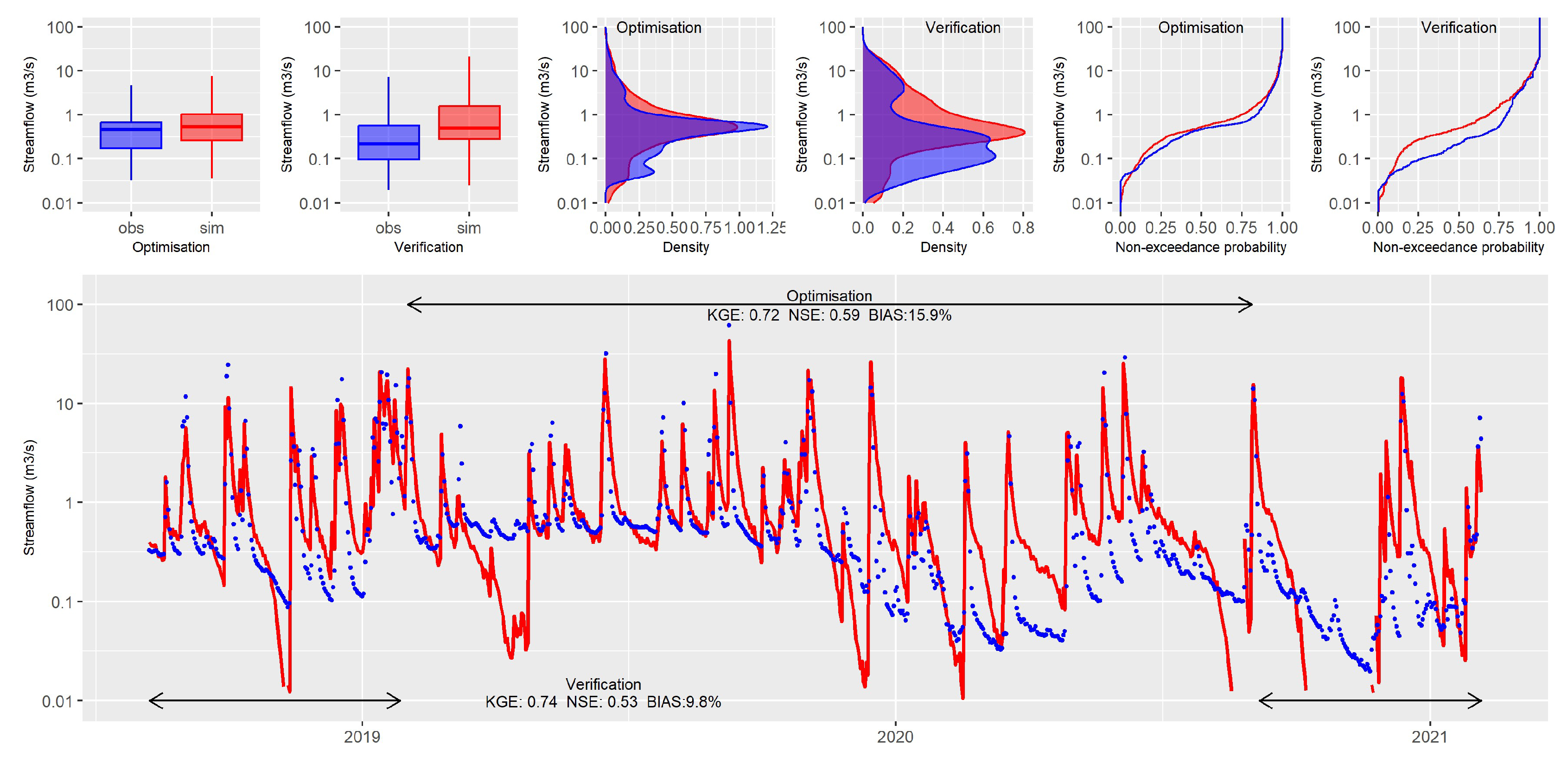
Figure 3.
Hydrographs of groundwater levels and scatter plot of observations and simulations.
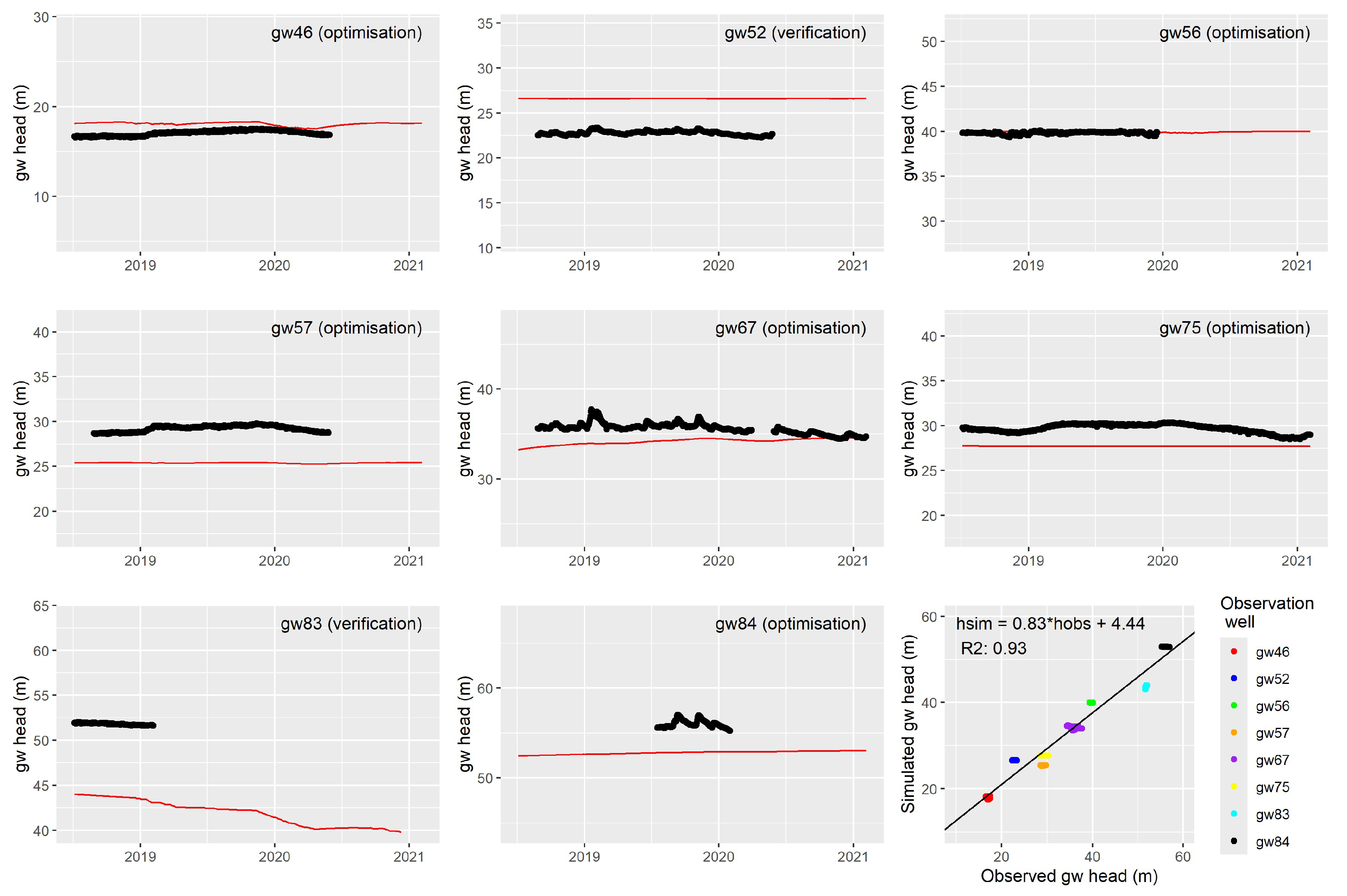
Figure 4.
Irrigation expansion effect on (a) groundwater head, (b) mean annual baseflow, (c) mean annual pumping rates, (d) mean annual groundwater-surface water exchange, and (e-f) flow duration curves.
Figure 4.
Irrigation expansion effect on (a) groundwater head, (b) mean annual baseflow, (c) mean annual pumping rates, (d) mean annual groundwater-surface water exchange, and (e-f) flow duration curves.
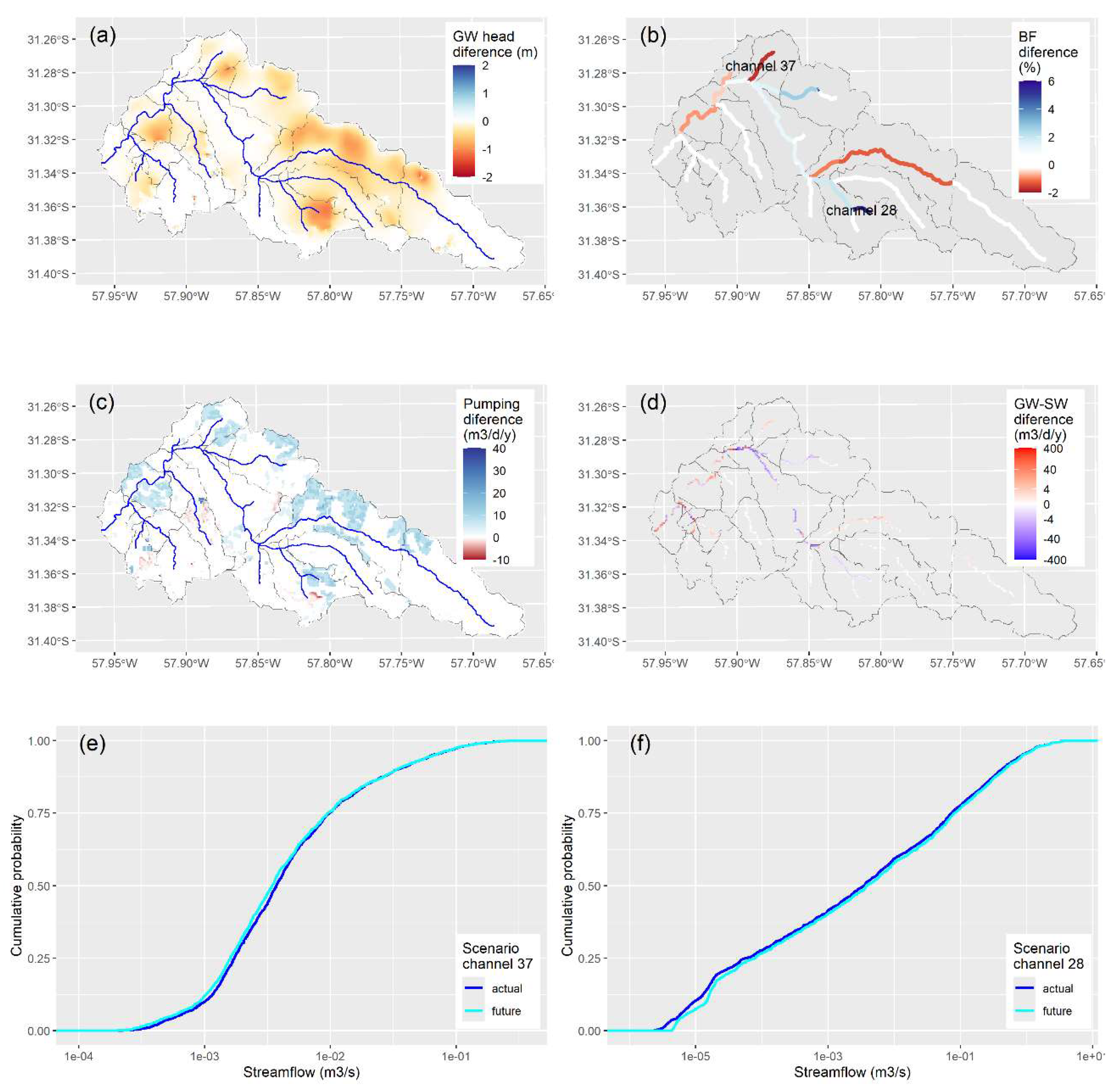

Table 1.
Optimization parameter for the 1st phase (total streamflow).
| Parameter | Description | File | Range | Type of change | Best fit |
|---|---|---|---|---|---|
| cn | Curve number compensation factor for soil group A, B, C and D [-] | cntable.lum | 0.9-1.1 | multiplicative | 0.937 |
| soil_k | Saturated hydraulic conductivity of soil | soil.sol | 0.7-1.3 | multiplicative | 1.07 |
| dp | Depth of the soil in the uper region | 0.7-1.3 | multiplicative | 1.08 | |
| epco | Plant uptake compensation factor | hydrology.hyd | 0.01-1 | substitutive | 0.92 |
| esco | Soil evaporation compensation factor | 0.01-1 | substitutive | 0.103 | |
| perco | Percolation coefficient | 0-1 | substitutive | 0.568 | |
| latq_co | Lateral flow coefficient | 0.01-0.99 | substitutive | 0.265 | |
| surq_lag | Surface runoff lag coefficient | parameter.bsn | 1-24 | substitutive | 2.03 |
Table 2.
Optimization parameters of 2nd phase (groundwater + baseflow).
| Parameter | Description | File | Range | Type of change | Best fit |
|---|---|---|---|---|---|
| specific yield | Usable water released from an aquifer per unit volume when drained by gravity [-] | gwflow.input | 0.2-0.35 | substitutive | 0.35 |
| aquhydracond | Aquifer hydraulic conductivity factor [-] | 0.5-1.95 | multiplicative | 1.63 | |
| sbedhydracond | Stream bed hydraulic conductivity [m/d] | 0.1-50 | substitutive | 1.48 | |
| sbedthick | Sream bed thickness [m] | 0.5-2 | substitutive | 1.94 | |
| w_stress_citr | Water stress for irrigated citriculture [-] | lum.dtl | 0.5-1 | multiplicative | 0.51 |
| w_stress_ofcp | Water stress for open field horticulture [-] | 0.5-1 | multiplicative | 0.85 | |
| w_stress_ghcp | Water s tress for greenhouse horticulture [-] | 0.5-1 | multiplicative | 0.57 |
Disclaimer/Publisher’s Note: The statements, opinions and data contained in all publications are solely those of the individual author(s) and contributor(s) and not of MDPI and/or the editor(s). MDPI and/or the editor(s) disclaim responsibility for any injury to people or property resulting from any ideas, methods, instructions or products referred to in the content. |
© 2025 by the authors. Licensee MDPI, Basel, Switzerland. This article is an open access article distributed under the terms and conditions of the Creative Commons Attribution (CC BY) license (http://creativecommons.org/licenses/by/4.0/).
Copyright: This open access article is published under a Creative Commons CC BY 4.0 license, which permit the free download, distribution, and reuse, provided that the author and preprint are cited in any reuse.


