Submitted:
04 February 2025
Posted:
05 February 2025
You are already at the latest version
Abstract
Ultrashort-laser-pulse-shape instability meters do not exist, so this task necessarily falls to pulse-measurement devices, like Frequency-Resolved Optical Gating (FROG) and its variations, which have proven to be a highly reliable class of techniques for measuring ultrashort laser pulses. Multi-shot versions of FROG have also been shown to sensitively distinguish trains of stable from those of unstable pulse shapes by displaying readily visible systematic discrepancies between the measured and retrieved traces in the presence of unstable pulse trains. However, the effects of pulse-shape instability and algorithm stagnation can be indistinguishable, so a never-stagnating algorithm—even when instability is present—is required and is in general important. In previous work, we demonstrated that our recently introduced Retrieved-Amplitude N-grid Algorithmic (RANA) approach produces highly reliable (100%) pulse-retrieval in the second-harmonic-generation (SHG) version of FROG for thousands of sample trains of pulses with stable pulse shapes. Further, it does so even for trains of unstable pulse shapes and thus both reliably distinguishes between the two cases and provides a rough measure of the degree of instability as well as a reasonable estimate of most typical pulse parameters. Here, we perform the analogous study for the polarization-gating (PG) and transient-grating (TG) versions of FROG, which are often used for higher-energy pulse trains. We conclude that PG and TG FROG, coupled with the RANA approach, also provide reliable indicators of pulse-shape instability. In addition, for PG and TG FROG, the RANA approach provides an even better estimate of a typical pulse in an unstable pulse train than SHG FROG does, even in cases of significant pulse-shape instability.
Keywords:
ultrashort
; ultrafast
; pulse
; FROG
1. Introduction
Amplified ultrashort laser pulses are in widespread use for the study of numerous phenomena and have provided important insights across many disciplines. Whether a study involves single-shot or multi-shot excitation of an effect, pulse-train stability is essential for optimal performance in any application. In other words, such measurements require consistency not only in the pulse energy but also in the pulse shape, i.e., its intensity and phase evolution during the pulse. For instance, high harmonic generation, which serves as the foundation for many important disciplines, including attosecond light sources [1], ultrafast optoelectronics [2], and attosecond spectroscopy [3,4,5], demands high stability in all pulse characteristics. Moreover, spectroscopic methods [6,7,8,9,10,11,12,13] use ultrashort pulses to enable the exploration of fundamental properties of matter, such as transient photo-induced phenomena, electronic structure, the dynamics of bound and free electrons, quantum coherence, and quantum spin, all of which require pulse-train stability to prevent fluctuating excitations of the sample with each pulse, especially when nonlinear dependencies or small temporal or spectral variations in the ultrashort pulse are being investigated [14]. The generation of ultrashort pulses at exotic wavelengths requires pump lasers, i.e., optical parametric oscillators and amplifiers, whose stability is especially consequential as the output pulses are nonlinearly dependent on the properties of the input light. Stable pump lasers are necessary to achieve consistent supercontinuum using optical fibers, in particular, hollow-core fibers [15,16], and for applications in high-intensity (>TW) ultrashort pulses, especially as the repetition rates and average power of these systems continue to increase [17]. Indeed, the medical [18,19,20,21,22] and industrial [23,24] domains now rely on amplified ultrashort laser pulse trains for surgical procedures, imaging, and micro-fabrication, including ultrashort pulse ablation manufacturing [25,26,27], selective laser-induced etching [28] and powder bed alloy fusion [29,30].
Furthermore, existing short-pulse petawatt-class lasers have now demonstrated new high-intensity laser-matter interactions that lead to secondary sources of high-energy photons [31] neutrons [32], and charged particles [33,34,35], with applications to medical imaging [36], cancer radiotherapy [37], multi-modal radiography [38] and tomography [39], and even fast ignition for inertial fusion energy [40,41]. Looking into the future, the realization of the necessary secondary source flux for such applications will require petawatt lasers with high average power (100s kW) and increasing repetition rates (>kHz [42,43]). Over the last few years, high intensity (>1018 W/cm2), higher repetition rate (10-50Hz) laser systems have been commissioned [44,45] and are now online [17,46], with 10kHz high-average-power petawatt systems now designed [47]. A central need for these high average power systems as their repetition rates approach the MHz level is rapid characterization and feedback [48] to ensure the highest quality pulse trains and the most stable performance. In all the above applications, laser pulse-shape stability is crucial to ensure reliable secondary source generation.
Unfortunately, amplified ultrashort-laser pulses are often plagued by instability, which can be due to a number of factors, including thermal fluctuations, unstable pump sources, inconsistent mode locking, vibrational pointing jitter, and turbulence in the surrounding air, to name only a few such culprits. The resulting instability tends to be more prevalent in laser systems with higher energies and shorter pulses, and it is especially pronounced in cutting-edge laser systems that advance ultrashort-pulse technology, such as few-cycle-pulse systems and lasers at atypical wavelengths.
From the birth of the field of ultrafast optics, shot-to-shot variations in the pulse shape, that is, the intensity-and-phase vs. time, of such laser pulses have presented a particularly difficult challenge for ultrashort-pulse laser measurement [49,50]. When faced with a train of pulses with unstable pulse shapes, the temporal intensity autocorrelation (the first method for measuring ultrashort pulses) produces a broad background with a narrow spike atop it. The width of this spike, which has come to be known as the coherence spike or coherent artifact, corresponds only to the potentially much shorter coherent temporal component of the unstable pulses in the train. The coherent artifact is therefore shorter than the typical pulse in the unstable train. While it is an obvious spikelike feature when the instability is significant, it can actually be quite misleading when the instability is not so significant; in this case, it may blend into the rest of the trace, resulting in a mistakenly short pulse length by a factor of two or more, as well as the mistaken conclusion of a stable pulse shape.
While it is now possible to measure the complete intensity and phase vs. time for a stable pulse train [51], many such measurement techniques have not been thoroughly studied for the case of pulse-shape instability and, unfortunately, like autocorrelation, can be badly confused by it. Currently, no device dedicated to the independent verification of pulse-shape instability exists, and, as a result, the responsibility of identifying the existence, severity, and kind of instability falls to the pulse-measurement methods themselves, which are not, in general, designed for this challenge. As a result, insufficient progress has been made in addressing this problem, and recent work [52,53,54,55,56] has revealed, among other results, the startling fact that, in the presence of pulse-shape instability, some widely used (mostly interferometric) methods measure only the coherent artifact.
There are numerous complications in attempting to measure such an unstable pulse train by any technique, as all measurement techniques necessarily provide a single resulting pulse from a given measured trace, and no one pulse can properly represent the many possible different pulses over which a measurement is made. As a result, the task is fundamentally impossible, and one must settle for quantities that are in some sense averaged. Unfortunately, this can yield results that are of little to no value.
Over the centuries, traditional spectrometers have provided a simple “average” spectrum. Of course, such measurements average out any spectral structure and so necessarily deliver a smoother spectrum than is in fact present. An extreme example of the highly misleading information provided by such a measurement is the multi-shot spectrometer measurement of the spectrum of a supercontinuum pulse from microstructure fiber, which yielded an extremely smooth spectrum, despite the fact that each individual pulse spectrum was wildly different and actually comprised over a thousand sharp spikes [58,59].
As a result, a typical spectrum, which often differs significantly from the average spectrum, could be, and often is, significantly more complex, but it would be much more informative. Remarkably, in the above-mentioned study, the Cross-correlation Frequency-Resolved Optical Gating (XFROG) technique [58,59] used to measure the continuum averaged over 100 billion pulses but nevertheless actually provided such a typical spectrum. As a result, XFROG has become the standard method for measuring such light pulses.
The spectral phase requires even more significant consideration. It is well known that, for a given spectrum, the shortest pulse corresponds to a spectral phase that is flat, while that of a longer, typically more complex, pulse is necessarily complex. Of course, simply averaging the spectral phase over many pulses with random complex spectral phases will, like a spectrometer-measured spectrum, also yield a much simpler and smoother curve, indeed, often a flat spectral phase. As a result, measuring the average spectral phase of an unstable pulse train usually erroneously yields the shortest possible pulse for a given measured spectrum (which, by the way, is also usually averaged over many pulses in these methods and so is also anomalously smooth). Indeed, measuring the average spectral phase will always yield a pulse that is shorter than any of the individual pulses in the train, and often by a large factor. In other words, the average spectral phase is the frequency-domain description of the coherent artifact.
As a result, it is crucial that a pulse-measurement technique not provide an average spectral phase, which is an essentially useless quantity. If it does, it will invariably yield a shorter pulse than is, in fact, present—unless the pulse train is perfectly stable (and spatially uniform). Indeed, such a method will be unable to differentiate a stable train of short, simple pulses from an unstable train of long, complicated pulses—the best- and worst-case scenarios, respectively, for most applications. Although critically important, this issue is often overlooked and/or poorly understood, and several popular techniques currently in use (and in use for decades) suffer from precisely this problem [52,53,54,55,56]. As with the spectrum, but much more importantly here, a pulse-measurement technique should ideally provide a typical spectral phase, or at least a phase as close as possible to it, which, coupled with a typical spectrum, would then more accurately reflect the average pulse length in time. If this is not possible (and it usually isn’t), the measurement should at least provide a typical pulse length.
Although single-shot measurement is the obvious solution to this problem, it is not possible for many laser systems, especially high-repetition-rate systems, for which even the shortest camera exposure times still capture multiple pulses in the train. And spatially averaging these quantities over a spatially complex beam would likely have precisely the same smoothing effect (although this effect has not been studied). Fortunately, some progress has been made: we earlier demonstrated that discrepancies between measured and retrieved Frequency Resolved Optical Gating (FROG) traces turn out to be a good indicator of instability. [58,59] They are a beneficial result of FROG’s overdetermination of the pulse: FROG’s N×N data array is used to measure only 2N pulse parameters. So, a trace that averaged over many different pulses cannot correspond to a single pulse. This has turned out to be a very helpful feature, allowing FROG to indicate instability by the presence of systematic discrepancies between measured and retrieved FROG traces.
Unfortunately, possible pulse-retrieval algorithm stagnation can also yield similar discrepancies. Even in the absence of instability, iterative algorithms and, in particular, FROG’s standard Generalized Projections (GP) algorithm can stagnate for complex pulses, yielding a retrieved pulse that bears little resemblance to a typical pulse and also depends on the initial guess. So, distinguishing between pulse-shape instability and algorithm stagnation—two very different issues—as the cause of such trace discrepancies is critical.
This has required us to redefine what we mean by algorithm “convergence” when dealing with pulse-shape instability [60]. In the absence of instability, convergence is easy to identify: the only differences between the measured and retrieved traces are due to random noise in the measured trace. And stagnation can be easily visually identified by the presence of systematic errors in the difference between the two traces (assuming that the measurement was made correctly).
In the presence of instability, however, the convergence concept is more subtle. In this case, stagnation, as we recently defined it [60], occurs when the RMS difference between the measured and retrieved traces, usually referred to as G, is higher than the lowest achievable G value for the given measured trace. But what is this latter value? Determining it requires running the relevant FROG algorithm numerous times (assuming that the algorithm converges at least once, which nearly always occurs in FROG in practice). The pulse with the lowest value of G is declared the converged case and hence the best estimate of the typical pulse. Then comparing its trace with the measured trace, it is evident that the more systematic error between the two traces the more instability is present. This is reasonable, but, unfortunately, running an algorithm many times is neither convenient nor always completely convincing.
What is needed is an algorithm that always converges to the lowest possible G value, even in the presence of instability in the first place. Fortunately, in previous work, we showed that this can be done for the second-harmonic-generation (SHG) version of FROG. Specifically, we demonstrated that our recently introduced Retrieved-Amplitude N-grid Algorithmic (RANA) approach [61,62,63] not only achieves extremely reliable (100%) pulse-retrieval in SHG FROG for trains of stable pulse shapes, even in the presence of noise, but also does so for unstable pulse trains and so reliably distinguishes between trains of stable and unstable pulse shapes. It also provides a reasonable estimate of the average pulse length, spectral width, and time-bandwidth product (TBPrms) in the train. This is the case because the RANA approach is extremely reliable and, in studies involving tens of thousands of simulated pulses, even in the presence of significant noise, has never stagnated. And specifically, we showed that it also did not stagnate even in the presence of pulse-shape instability [53]. It also provided many of the characteristics of a “typical” pulse in the unstable train [57] (although it tended to under-estimate the amount of typical pulse structure).
As a result, an analogous never-stagnating algorithm—even in the presence of instability—is also highly desirable for the versions of FROG that are generally used to measure amplified pulses. These include the polarization-gating (PG) and transient-grating (TG) FROG variants (which are highly desirable because they effectively eliminate the direction-of-time ambiguity of SHG FROG). Additionally, PG FROG is automatically phase-matched, and TG FROG is broadly phase-matched, so both are not usually limited by the pulse’s bandwidth.
PG FROG and the more common version of TG FROG are mathematically equivalent. The mathematical relation for their measured trace is:
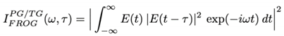 (1)
where E(t) is the pulse’s complex electric field as a function of time, t. Also, ω is the angular frequency, and τ is the delay between the pulses.
(1)
where E(t) is the pulse’s complex electric field as a function of time, t. Also, ω is the angular frequency, and τ is the delay between the pulses.
(1)
As a result, as we did for SHG FROG, we here consider trains of unstable complex pulses measured by PG and TG FROG using the analogous RANA approach for them. And we compare the performance of the RANA approach to that of the well-known generalized-projections (GP) algorithm without the RANA improvements for these two FROG beam geometries. We find, for these FROG variations, that the standard GP algorithm also often fails to converge for unstable pulse trains (as it occasionally does for complex stable ones), yielding variable and hence potentially confusing trace discrepancies. As a result, it is an imperfect indicator of instability. But we find that the RANA approach, on the other hand, yields minimal trace discrepancies for all the cases considered, that is, zero stagnations, even for highly unstable pulse trains. It also yields accurate pulse parameters, as well as much of the structure of a typical pulse. We conclude that PG and TG FROG, coupled with the RANA approach, like SHG FROG with RANA, provide highly reliable indicators of pulse-shape instability. And we find that PG/TG FROG yield an even better estimate of a typical pulse in the train, even in cases of high instability.
2. Simulations
For better comparison with our previous work on SHG FROG, we used the same test pulses as in those previous simulations, in which we generated three pulse trains, each containing 5000 unique pulses, as discussed in that work [60]. Each pulse was constructed with a stable short pulse plus a longer unstable component [53]. The temporal full width at half-maximum (FWHM) of the stable component was set at 12 fs for all three trains. Because the random components were longer, they were assigned higher energies before being added to the stable train, resulting in average temporal FWHMs of 26, 54, and 108 fs for the unstable trains. The pulse energies were then tailored to match a normal distribution with a coefficient of variation of 10%. Simulations of PG and TG FROG measurements were created by taking the mean of the individual pulses in each of the three trains. Additionally, 3% additive and 5% multiplicative noise [64] were applied to the traces. Also, before the retrieval process, the random trace noise was suppressed using the same preprocessing techniques as are always performed when retrieving pulses from experimental traces [58].
We generated three multi-shot simulated measured PG/TG FROG traces by adding together the 5000 traces of all the pulses for each of the three trains. We then retrieved pulses from the three resulting traces using both the standard GP algorithm and the RANA approach [62] (which incorporated the GP algorithm), each with 100 different initial guesses. For the pulse trains with average temporal FWHMs of 26, 54, and 108 fs, we used trace sizes of 128 × 128, 256 × 256, and 512 × 512, respectively, ensuring that the intensities at the trace perimeters were less than 10−4 of the maximum intensity. We then calculated the G and G’ errors (non-normalized and normalized rms difference between measured and retrieved traces, respectively), the TBPrms, and the temporal FWHMs of the retrieved fields for the three unstable trains. The maximum number of iterations was set to 1500 for the GP algorithm and 375 for the RANA approach. Iterations were stopped when the average change in G error values over the previous ten iterations was less than 10−7.
We evaluated the performance of the GP and RANA approaches by comparing their G’ errors. Recall that RANA involves obtaining a significantly improved initial-guess for the pulse spectrum directly from the measured trace and also using a multi-grid approach for the iterations, using only small numbers of the trace data points for early iterations and only using the entire trace for the final few. [62] The quantity of first guesses and iterations are shown horizontally in Table 1. Each row indicates the values used for a different pulse train.
3. Results
As mentioned earlier, if an algorithm reliably converges, even in the presence of instability, we would expect it to achieve the minimum G or G’ error for all reasonable initial guesses. If not, then we would expect to see variations in these values depending on the initial guess. Figure 1 depicts all the G’ errors obtained from 100 runs using both the standard GP algorithm and RANA approach on noisy traces.
These results clearly illustrate that the RANA approach converges to the smallest value of G’ for all runs and for all instability values. In other words, it converged in all cases. In contrast, the standard GP algorithm does fairly well for the least unstable pulse train, but, for increasing instability, it shows significant variability in the resulting G’ errors, often requiring multiple attempts to achieve the minimum achievable G’ error. For pulse trains with an average temporal FWHM of 26 fs, the standard GP algorithm successfully converged to acceptable pulses with traces closely matching the measured ones in 92% of the trials. This performance decreased to 86% and 44% for pulse trains with average FWHMs of 54 fs and 108 fs, respectively, that is, more instability. While this performance is not perfect and quite undesirable for the less stable trains, it is nevertheless considerably better than that of GP for SHG FROG that we found in our previous study [60].
It is important to note that, in our studies, the impact of trace noise was minor compared to that of pulse-shape instability. As is well known, random noise in FROG traces can be minimized using simple preprocessing. In stable pulse trains, the converged G’ error should, and does, align with the average random noise remaining in the measured trace after preprocessing; G’ errors larger than this necessarily indicate pulse-train instability, at least for the RANA approach. For the standard GP algorithm, these discrepancies are a sum of stagnation and instability effects, and the best way to distinguish them using the standard GP algorithm at this time appears to be running the algorithm many times and using the result with the smallest G or G’ error, as we have done here and as is often done in practice. Of course, this is far less desirable than running a more reliable algorithm only once.
Figure 2a shows the resulting multi-shot trace of train #3. Note the obvious thin vertical line in it, i.e., the coherent artifact, which is intimately related to that of autocorrelation (recall that FROG is a spectrally resolved autocorrelation). Of course, while FROG traces exhibit this artifact, this does not pose a problem in FROG, first because its presence alerts the algorithm and the user (as for autocorrelation) to the instability, and our results confirm this. Also, as such an artifact cannot occur in a stable-pulse or single-pulse FROG trace, all FROG algorithms necessarily ignore it, using it and other information in the trace to retrieve the best possible typical pulse, as we found in our earlier work for SHG FROG [60]. This is also illustrated in the worst-case retrieved traces for both algorithms we studied, shown in Figure 2b,c, where no such vertical line appears for either algorithm. In other words, even in the worst cases, no such artifact occurs in retrieved traces. Do note, however, that the standard GP algorithm is somewhat confused by this effect and retrieves a pulse with a larger area, that is, a larger TBP. This occurs, not only for the worst case, but also for the average retrieved pulse for GP. The RANA approach does much better and returns fairly accurate TBPs in all three cases.
Figure 2d-g show every retrieved pulse field using both the GP algorithm (d,f) and the RANA approach (e,g) from a randomly chosen noisy trace of train #3, with 108 fs average temporal FWHM. The standard GP algorithm yields a variety of pulse shapes, based to some extent on the initial guess, with GP-retrieved pulses showing a large range of variations in the temporal and spectral FWHMs. Additionally, the worst-case (and many other unshown) GP-retrieved traces bear no resemblance to the measured trace. In contrast, pulses retrieved using the RANA approach, although somewhat less structured than the actual pulses, do show some of the typical pulse structure and have pulse lengths and spectral widths that closely match those of the measured pulses in the unstable train. Although we should have no expectation of convergence to identical pulses on all runs of any algorithm in the presence of instability, when the trace corresponds to no single pulse, impressively, the maximum and minimum pulse lengths retrieved by RANA are quite similar, indicating that, even in the presence of instability, it achieves a reasonable “typical” pulse length.
Table 2 shows the average G′ errors and TBPs for the 100 RANA and GP retrievals from the various FROG traces. For the least unstable case, the two approaches yield similar results, indicating that the standard GP algorithm performs reasonably well for somewhat complex and unstable pulse trains. But, for the two most unstable trains, RANA yields smaller TBPs and standard deviations than GP, indicating both better convergence and also less variations in the retrieved pulses. The larger standard deviations of the TBP values of the standard GP algorithm indicate that, when convergence is not achieved, the retrieved fields exhibit significant variations, resulting in inconsistent and arguably unreliable results.
Figure 3 plots the RMS time-bandwidth product (TBPrms) against the G’ error for all of the retrieved pulses using both the GP and RANA approach. Because we used the same pulse trains in this simulation as in our previous work, the average theoretical pulse length and TBPrms values for the fluctuating pulses of the trains were the same, with averages of τFWHM = 26, 54, and 108fs and TBPrms of 1.97, 4.75, and 9.28, respectively. When convergence is achieved with either the RANA approach or the GP algorithm, the TBPrms values align well with the actual values. However, Figure 3 also indicates that stagnated results from using the standard GP algorithm can lead to TBPrms values that do not accurately reflect the average TBPrms of the pulses within the train, with discrepancies increasing with increasing instability.
As discussed in our previous work [63], the RANA approach uses four directly retrieved approximate spectra to produce the initial guesses from the measured trace for input into the iterative process, and we also did this in this study of PG/TG FROG. Note that these directly retrieved spectra serve only as initial guesses for the algorithm and need not be very accurate. In the absence of instability, such spectra usually accurately approximate the pulse spectrum, but, in the presence of instability, they instead reflect the average spectrum. This is to be expected, but it could, in principle, degrade the performance of the RANA approach. However, RANA’s other advantageous features appear to compensate for this averaging. Also, the average spectrum, whose width is fairly accurate, is still a better initial guess than noise, the usual initial guess for standard GP. Figure 4 plots the average spectra of the trace along with the first choices among these four retrieved spectra.
It is important to note that the mean retrieval times for traces with instability are significantly longer than those for stable trains for all algorithms. This is because convergence rates are slower when the trace does not match an actual pulse, requiring more iterations for the algorithm to converge. However, the average retrieval time for the RANA approach is less than that for the GP algorithm, even in cases where the GP algorithm converges.
4. Conclusions
In this study, we explored the convergence behavior of the standard GP algorithm and the recently introduced RANA approach for PG/TG FROG traces averaged over trains of pulses with unstable shapes and hence with coherent artifacts. As expected, we found that instability yields PG/TG FROG traces that do not correspond to traces from single pulses, which implies that these techniques are very useful for identifying instability, in addition to measuring the pulse intensity and phase vs. time. But we found that the standard GP algorithm often fails to clearly distinguish between discrepancies caused by instability artifacts and those due to algorithm stagnation, making it difficult for it to identify instability accurately. This necessitates multiple retrieval attempts to find the lowest G error, with no definitive way to determine if the discrepancies are due to instability or algorithm stagnation.
In contrast, our results show that, for traces of trains with unstable pulse shapes, the RANA-retrieved trace consistently achieves the minimum discrepancy with the measured trace, resulting in the lowest G’ error, that is, converges in all cases that we considered. Thus the RANA approach, established to have 100% reliability with stable pulses, also proves highly effective in evaluating pulse-train stability. This reliable convergence indicates that any discrepancies between the measured and retrieved traces are due to pulse-shape fluctuations, and not algorithm stagnation. Moreover, the retrieved field accurately reflects the average pulse length, spectral width, and TBP of the pulses in the train, providing the best available depiction of a typical pulse, although with somewhat less structure. It also provides some of the structure present in a typical pulse in the train.
In summary, the RANA approach offers the most reliable FROG pulse-retrieval approach for both stable and unstable pulse trains, making it a highly reliable gauge of the average pulse length, TBP, and pulse-train stability or instability and, of course, the precise pulse intensity and phase vs. time and frequency for stable pulse trains. As no other pulse-measurement technique has, to our knowledge, been shown to possess all of these characteristics, RANA (in particular, in conjunction with PG/TG FROG) yields the best general performance of all existing pulse-measurement techniques.
Finally, it is worth considering possible future effort on this subject. First, performing this analysis on larger sets of pulse trains would be helpful, as is always the case for iterative algorithms. Also, additional versions of FROG, including those that use the nonlinear processes, self-diffraction (which is mathematically equivalent to the alternative arrangement of TG FROG, not considered herein) and third-harmonic generation, would also benefit greatly from the RANA approach, and their ability to reliably discern instability should be determined. Also, the RANA approach can utilize any FROG algorithm (not just GP) as its kernel, and we believe that algorithm performance for both stable and unstable trains would be vastly improved using it in conjunction with those algorithms. Lastly, no technique, including that described herein, can determine the precise type of instability present in the pulse train. As the parameter space involved in such a study is vast, this is a challenge that is unlikely to be achieved any time soon, but we mention it here to inspire future generations.
Author Contributions
R.T. conceived the idea and directed the project. R.J. performed the numerical calculations and analyzed the results. All authors contributed significantly to the preparation of the manuscript. All authors discussed the results and gave their approval to the final version. The authors would like to point out that this paper extends the approach discussed in a previous paper for the SHG FROG technique to the PG and TG FROG techniques. As the motivation for and description of the simulations are the same, it is important that our descriptions of the simulations be similar. So some text has been paraphrased from that paper, as to do otherwise would imply differences between the works that do not exist. Of course, the science of the two works is different.
Funding
National Science Foundation #ECCS-1609808; Georgia Research Alliance. This work was completed under the auspices of the U.S. Department of Energy by Lawrence Livermore National Laboratory under contract DE-AC52-07NA27344.
Data Availability Statement
Data underlying the results presented in this paper are not publicly available at this time but may be obtained from the authors upon reasonable request.
Conflicts of Interest
R.T. owns a company that sells pulse measurement devices, although not the algorithm described herein. R.J. consults for this company. E.G. does not have any conflict of interest.
References
- Midorikawa, K. Progress on table-top isolated attosecond light sources. Nat Photonics 2022, 16, 267–278. [Google Scholar] [CrossRef]
- Sengupta, K.; Nagatsuma, T.; Mittleman, D.M. Terahertz integrated electronic and hybrid electronic–photonic systems. Nat Electron 2018, 1, 622–635. [Google Scholar] [CrossRef]
- Goulielmakis, E.; et al. Real-time observation of valence electron motion. Nature 2010, 466, 739–743. [Google Scholar] [CrossRef] [PubMed]
- Luu, T. T.; et al. Extreme ultraviolet high-harmonic spectroscopy of solids. Nature 2015, 521, 498–502. [Google Scholar] [CrossRef]
- Li, J.; et al. Attosecond science based on high harmonic generation from gases and solids. Nat Commun 2020, 11, 2748. [Google Scholar] [CrossRef]
- Kobayashi, T. Development of Ultrashort Pulse Lasers for Ultrafast Spectroscopy. Photonics 2018, 5, 19. [Google Scholar] [CrossRef]
- Kraus, P.M.; Zürch, M.; Cushing, S.K.; Neumark, D.M.; Leone, S.R. The ultrafast X-ray spectroscopic revolution in chemical dynamics. Nat Rev Chem 2018, 2, 82–94. [Google Scholar] [CrossRef]
- Picqué, N. & Hänsch, T. W. Frequency comb spectroscopy. W. Frequency comb spectroscopy. Nat Photonics 2019, 13, 146–157. [Google Scholar]
- Kuhs, C.T.; Luther, B.M.; Krummel, A.T. Recent Advances in 2D IR Spectroscopy Driven by Advances in Ultrafast Technology. IEEE Journal of Selected Topics in Quantum Electronics 2019, 25, 1–13. [Google Scholar] [CrossRef]
- Maiuri, M.; Garavelli, M.; Cerullo, G. Ultrafast Spectroscopy: State of the Art and Open Challenges. J Am Chem Soc 2020, 142, 3–15. [Google Scholar] [CrossRef]
- Pupeza, I.; Zhang, C.; Högner, M.; Ye, J. Extreme-ultraviolet frequency combs for precision metrology and attosecond science. Nat Photonics 2021, 15, 175–186. [Google Scholar] [CrossRef]
- Lloyd-Hughes, J.; et al. The 2021 ultrafast spectroscopic probes of condensed matter roadmap. Journal of Physics: Condensed Matter, 3530. [Google Scholar]
- Garratt, D.; et al. Direct observation of ultrafast exciton localization in an organic semiconductor with soft X-ray transient absorption spectroscopy. Nat Commun 2022, 13, 3414. [Google Scholar] [CrossRef] [PubMed]
- Turner, D.B.; Wilk, K.E.; Curmi PM, G.; Scholes, G.D. Comparison of Electronic and Vibrational Coherence Measured by Two-Dimensional Electronic Spectroscopy. J Phys Chem Lett 2011, 2, 1904–1911. [Google Scholar] [CrossRef]
- Corwin, K. L.; et al. Fundamental Noise Limitations to Supercontinuum Generation in Microstructure Fiber. Phys Rev Lett 2003, 90, 113904. [Google Scholar] [CrossRef]
- Adamu, A. I.; et al. Noise and spectral stability of deep-UV gas-filled fiber-based supercontinuum sources driven by ultrafast mid-IR pulses. Sci Rep 2020, 10, 4912. [Google Scholar] [CrossRef]
- Haefner, C. L.; et al. High average power, diode pumped petawatt laser systems: a new generation of lasers enabling precision science and commercial applications. in (eds. Korn, G. & Silva, L. O.) 1024102 (2017). [CrossRef]
- Fujimoto, J.; et al. Ultrashort Laser Pulses in Biology and Medicine. (Springer, 2008).
- Litvinova, K.; Chernysheva, M.; Stegemann, B.; Leyva, F. Autofluorescence guided welding of heart tissue by laser pulse bursts at 1550 nm. Biomed Opt Express 2020, 11, 6271. [Google Scholar] [CrossRef]
- Cheng, P.; et al. Direct control of store-operated calcium channels by ultrafast laser. Cell Res 2021, 31, 758–772. [Google Scholar] [CrossRef]
- Clough, M.; et al. Flexible simultaneous mesoscale two-photon imaging of neural activity at high speeds. Nat Commun 2021, 12, 6638. [Google Scholar] [CrossRef]
- Li, C.L.; Fisher, C.J.; Burke, R.; Andersson-Engels, S. Orthopedics-Related Applications of Ultrafast Laser and Its Recent Advances. Applied Sciences 2022, 12, 3957. [Google Scholar] [CrossRef]
- Orazi, L.; Romoli, L.; Schmidt, M.; Li, L. Ultrafast laser manufacturing: from physics to industrial applications. CIRP Annals 2021, 70, 543–566. [Google Scholar] [CrossRef]
- Bornschlegel, B.; Finger, J. In-Situ Analysis of Ultrashort Pulsed Laser Ablation with Pulse Bursts. Journal of Laser Micro/Nanoengineering.
- Ahmed, N.; Darwish, S.; Alahmari, A.M. Laser Ablation and Laser-Hybrid Ablation Processes: A Review. Materials and Manufacturing Processes 2016, 31, 1121–1142. [Google Scholar] [CrossRef]
- Ravi-Kumar, S.; Lies, B.; Zhang, X.; Lyu, H.; Qin, H. Laser ablation of polymers: a review. Polym Int 2019, 68, 1391–1401. [Google Scholar] [CrossRef]
- Kroger, M.; Lasogga, C.; Kratz, M.; Hinke, C.; Holly, C. Platform for Adaptive Integration of Data-Driven Models And Simulations Into Ultra Short Pulse Manufacturing Systems. Journal of Laser Micro/Nanoengineering.
- Hermans, M.; Gottman, J.; Riedel, F. Selective, Laser-Induced Etching of Fused Silica at High Scan-Speeds Using KOH. Journal of Laser Micro/Nanoengineering.
- Kotadia, H.R.; Gibbons, G.; Das, A.; Howes, P.D. A review of Laser Powder Bed Fusion Additive Manufacturing of aluminium alloys: Microstructure and properties. Addit Manuf 2021, 46, 102155. [Google Scholar] [CrossRef]
- Ullsperger, T.; et al. Ultra-short pulsed laser powder bed fusion of Al-Si alloys: Impact of pulse duration and energy in comparison to continuous wave excitation. Addit Manuf 2021, 46, 102085. [Google Scholar] [CrossRef]
- Albert, F.; et al. Characterization and applications of a tunable, laser-based, MeV-class Compton-scattering <math display="inline"> <mi>γ</mi> </math> -ray source. Physical Review Special Topics - Accelerators and Beams.
- Perkins, L. J.; et al. The investigation of high intensity laser driven micro neutron sources for fusion materials research at high fluence. Nuclear Fusion 2000, 40, 1–19. [Google Scholar] [CrossRef]
- Siders, C. W.; et al. Laser Wakefield Excitation and Measurement by Femtosecond Longitudinal Interferometry. Phys Rev Lett 1996, 76, 3570–3573. [Google Scholar] [CrossRef]
- Snavely, R. A.; et al. Intense High-Energy Proton Beams from Petawatt-Laser Irradiation of Solids. Phys Rev Lett 2000, 85, 2945–2948. [Google Scholar] [CrossRef]
- Jung, D.; et al. Efficient carbon ion beam generation from laser-driven volume acceleration. New J Phys 2013, 15, 023007. [Google Scholar] [CrossRef]
- Kieffer, J. C.; et al. Future of laser-based X-ray sources for medical imaging. Applied Physics B, 2002. [Google Scholar]
- Bulanov, S.V.; Khoroshkov, V.S. Feasibility of using laser ion accelerators in proton therapy. Plasma Physics Reports 2002, 28, 453–456. [Google Scholar] [CrossRef]
- Williams, G. J.; et al. Dual-energy fast neutron imaging using tunable short-pulse laser-driven sources. Review of Scientific Instruments.
- Svendsen, K.; et al. Optimization of soft X-ray phase-contrast tomography using a laser wakefield accelerator. Opt Express 2018, 26, 33930. [Google Scholar] [CrossRef]
- Robinson, A. P. L.; et al. Theory of fast electron transport for fast ignition. Nuclear Fusion 2014, 54, 054003. [Google Scholar] [CrossRef]
- Kemp, A.J.; Wilks, S.C.; Tabak, M. Laser-to-proton conversion efficiency studies for proton fast ignition. Phys Plasmas.
- Kling, M.; et al. 2023 Report on the Basic Research Needs Workshop on Laser Technology. ( 2023.
- Ma, T.; Betti, R.; Akli, K.; Van Dam, J. Report of the 2022 Fusion Energy Sciences Basic Research Needs Workshop. ( 2022.
- Reagan, B. A.; et al. High repetition rate, high energy petawatt laser for the matter in extreme conditions upgrade. in High Power Lasers for Fusion Research VII (eds. Haefner, C. L. & Awwal, A. A.) 17 (SPIE, 2023). [CrossRef]
- Green, J. T.; et al. Development of the L2-DUHA high repetition rate, 100 TW OPCPA system for laser wakefield acceleration. in Laser Congress D.C., 2023. [CrossRef]
- Schillaci, F.; et al. The ELIMAIA Laser–Plasma Ion Accelerator: Technological Commissioning and Perspectives. Quantum Beam Science 2022, 6, 30. [Google Scholar] [CrossRef]
- Galvin, T. C.; et al. Scaling of petawatt-class lasers to multi-kHZ repetition rates. in High-Power, High-Energy, and High-Intensity Laser Technology IV (eds. Butcher, T. J. & Hein, J.) 1 (SPIE, 2019). [CrossRef]
- Ma, T.; et al. Accelerating the rate of discovery: toward high-repetition-rate HED science. Plasma Phys Control Fusion 2021, 63, 104003. [Google Scholar] [CrossRef]
- Fisher, R.A.; Fleck, J.A. On the phase characteristics and compression of picosecond pulses. Appl Phys Lett 1969, 15, 287–290. [Google Scholar] [CrossRef]
- Trebino, R. The Most Important Paper You’ve Never Read. Opt Photonics News 2020, 31, 46–53. [Google Scholar] [CrossRef]
- RTrebino, R. Jafari, S. A. Akturk, P. Bowlan, Z. Guang, P. Zhu, E. Escoto, and G. Steinmeyer, "Highly Reliable Measurement of Ultrashort Laser Pulses," J. Appl. Phys. 128, 171103-171101 - 171103-171143 (2020).
- Ratner, J.; Steinmeyer, G.; Wong, T.C.; Bartels, R.; Trebino, R. Coherent artifact in modern pulse measurements. Opt. Lett. 2012, 37, 2874. [Google Scholar] [CrossRef]
- Rhodes, M.; Steinmeyer, G.; Ratner, J.; Trebino, R. Pulse-shape instabilities and their measurement. Laser Photon Rev 2013, 7, 557–565. [Google Scholar] [CrossRef]
- Rhodes, M.; Mukhopadhyay, M.; Birge, J.; Trebino, R. Coherent artifact study of two-dimensional spectral shearing interferometry. Journal of the Optical Society of America B 2015, 32, 1881. [Google Scholar] [CrossRef]
- Rhodes, M.; Guang, Z.; Trebino, R. Unstable and Multiple Pulsing Can Be Invisible to Ultrashort Pulse Measurement Techniques. Applied Sciences 2016, 7, 40. [Google Scholar] [CrossRef]
- Escoto, E.; Jafari, R.; Steinmeyer, G.; Trebino, R. Linear chirp instability analysis for ultrafast pulse metrology. Journal of the Optical Society of America B 2020, 37, 74. [Google Scholar] [CrossRef]
- Escoto, E.; Jafari, R.; Trebino, R.; Steinmeyer, G. Retrieving the coherent artifact in frequency-resolved optical gating. Opt Lett 2019, 44, 3142. [Google Scholar] [CrossRef]
- Trebino, R. Frequency-Resolved Optical Gating: The Measurement of Ultrashort Laser Pulses. (Kluwer Academic Publishers, 2002).
- Xu, L.; Zeek, E.; Trebino, R. Simulations of frequency-resolved optical gating for measuring very complex pulses. Journal of the Optical Society of America B, 2008. [Google Scholar]
- Jafari, R.; Khosravi, S.D.; Trebino, R. Reliable determination of pulse-shape instability in trains of ultrashort laser pulses using frequency-resolved optical gating. Sci Rep 2022, 12, 21006. [Google Scholar] [CrossRef]
- Jafari, R. , Jones, T. & Trebino, R. 100% reliable algorithm for second-harmonic-generation frequency-resolved optical gating. Opt Express 2019, 27, 2112. [Google Scholar]
- Jafari, R.; Trebino, R. Highly Reliable Frequency-Resolved Optical Gating Pulse-Retrieval Algorithmic Approach. IEEE J Quantum Electron 2019, 55, 1–7. [Google Scholar] [CrossRef]
- Jafari, R.; Trebino, R. Extremely Robust Pulse Retrieval From Even Noisy Second-Harmonic-Generation Frequency-Resolved Optical Gating Traces. IEEE J Quantum Electron 2020, 56, 1–8. [Google Scholar] [CrossRef]
- Fittinghoff, D.N.; DeLong, K.W.; Trebino, R.; Ladera, C.L. Noise sensitivity in frequency-resolved optical-gating measurements of ultrashort pulses. Journal of the Optical Society of America B 1995, 12, 1955. [Google Scholar] [CrossRef]
Figure 1.
G’ errors for retrieval of three noisy PG/TG FROG traces, which are contaminated with 3% additive and 5% multiplicative noise for three unstable pulse trains with an average temporal FWHM of (a) 26 fs, (b) 54 fs, and (c) 108 fs. The G’ errors are obtained from pulse recovery over 100 runs using the RANA approach (blue triangles) and the standard GP algorithm (red circles) on noise-filtered traces. The RANA approach consistently achieves the minimum G’ error, whereas the GP algorithm alone does not, necessitating additional algorithm runs in practice. In all six cases, the impact of random trace noise is small. On the other hand, in all cases, the effects of pulse-shape instability dominate, yielding the resulting large values of G’. However, stagnation contributes increasingly to the resulting values of G’ for the standard GP algorithm as instability increases. On the other hand, there is negligible contribution to G’ from stagnation in all three RANA cases. This is the main result of this work.
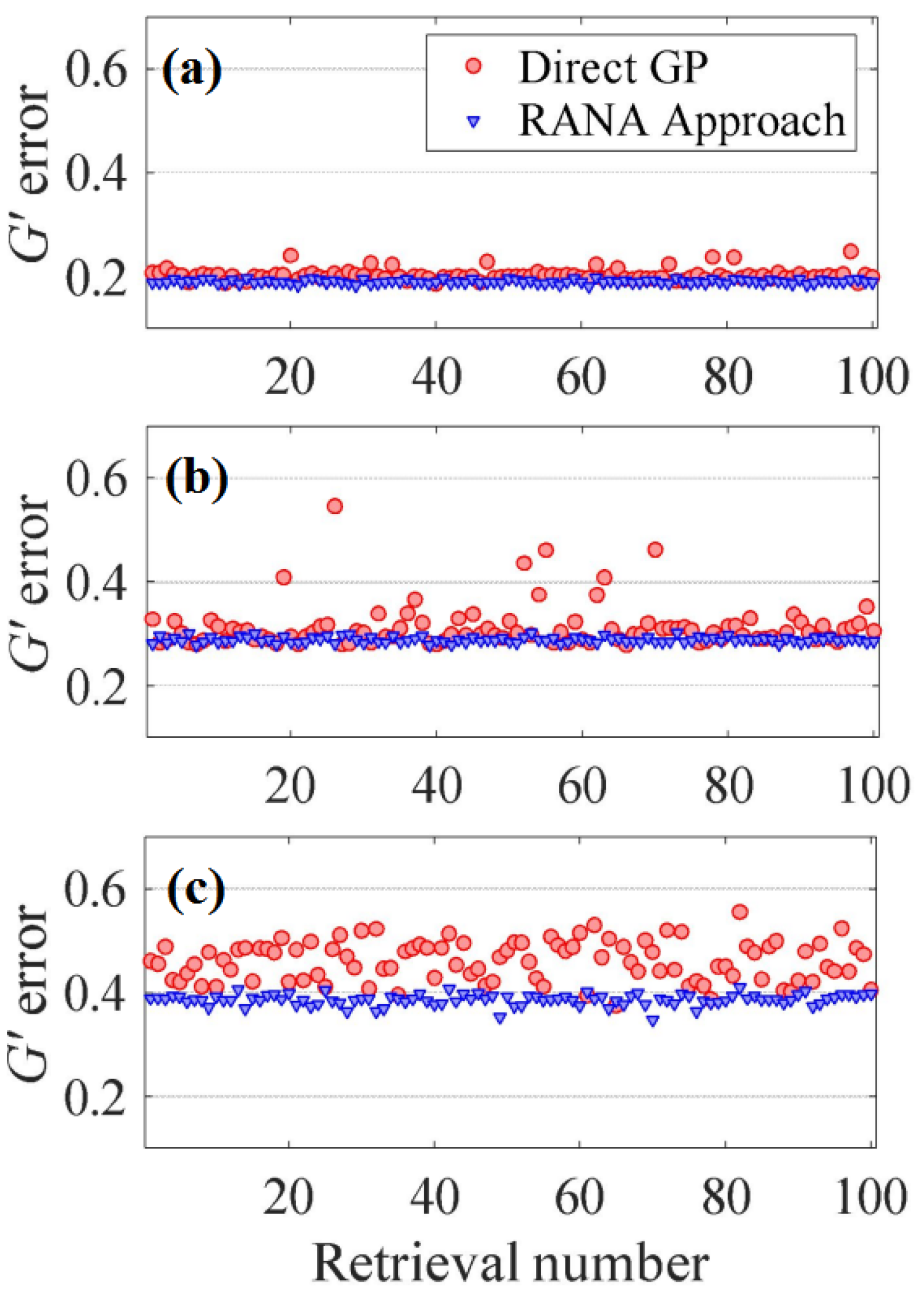
Figure 2.
(a) The trace generated by the unstable train of pulses with average temporal FWHM of 108fs. Note the narrow coherent artifact centered at zero delay. (b) The reconstructed trace obtained using the GP algorithm for the “worst-case retrieval,” for which the G’ error is the largest. (c) The “worst-case” retrieval from use of the RANA approach. Note the much smaller trace area and hence much smaller TBP for the RANA approach. (d and e) Two retrieved temporal intensities (both shown as dashed black and red dashed curves and corresponding to the maximum and minimum retrieved FWHMs) and all the retrieved phases (blue) for the GP algorithm (d) and RANA approach (e) are shown. Note the large differences between the two intensity curves for the GP algorithm in (d) and the much smaller, essentially indistinguishable intensity curves for the RANA approach in (e). The phase curves have arbitrary constants added to them in order to separate them, and those grouped together in the top of (d) correspond to the clearly stagnated results and are more complex on average than the converged results shown below them. (f) and (g) Analogous quantities for the spectra, except using green instead of red. In both figures, the spectra are difficult to distinguish because the stagnation in the GP approach is mainly manifested in the spectral phases. These effects will be more evident in the retrieved TBPs.
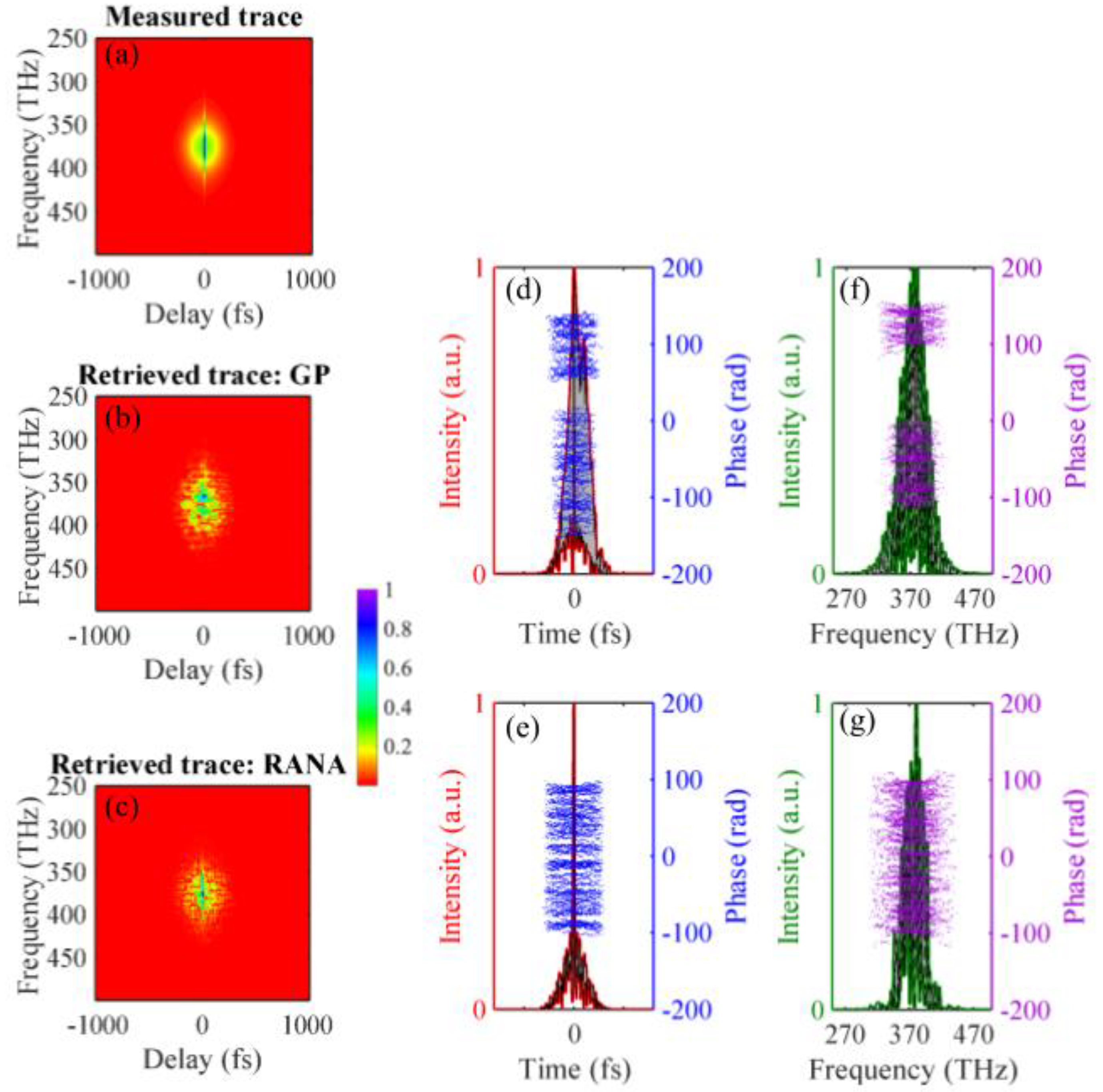
Figure 3.
The resulting TBPrms for the retrieved pulses using the GP algorithm and the RANA approach vs. G’ error, indicated by red and blue crosses, respectively. We find that the GP algorithm’s converged results yield TBPrms approximately equal to the average TBPrms of the pulse train, while the stagnated results have varying TBPrms, showing increasing values and variation for the more complex pulse trains, especially the most complex pulse train. The RANA approach’s retrieved fields are much more consistent and precise, and they better approximate the average values for the pulses in all three trains.
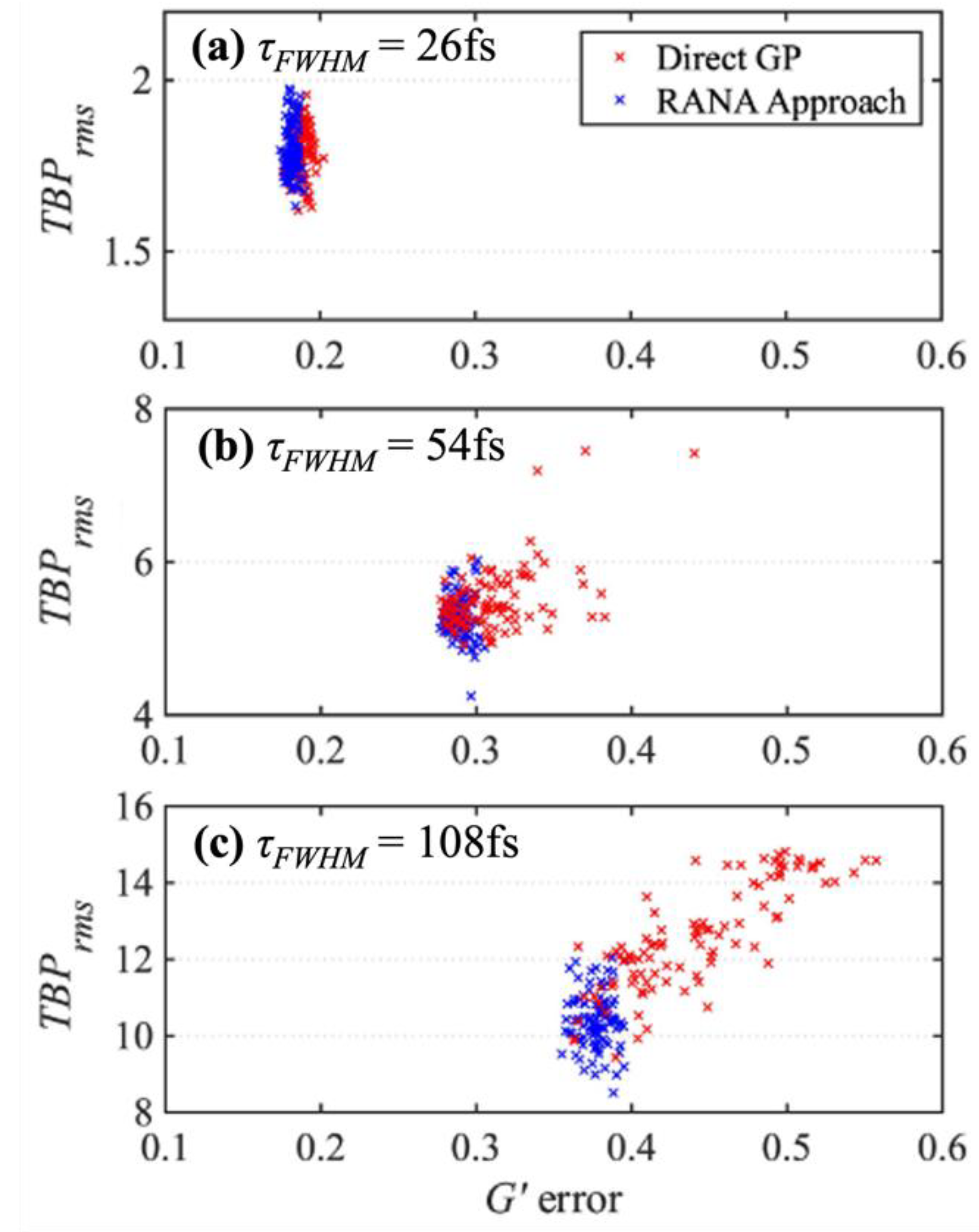
Figure 4.
The first and second columns show the typical spectra for trains 1 (top) to 3 (bottom). The third column plots the directly retrieved spectra from the marginal of the PG/TG FROG trace (obtained in and required for the RANA approach) alongside the average spectra – i.e., the spectrometer measurement – for the three trains with average (a) τFWHM = 26fs, (b) τFWHM = 54fs, and (c) τFWHM = 108fs. The retrieved spectra from PG/TG FROG trace marginal match the average spectra of the unstable pulse train.
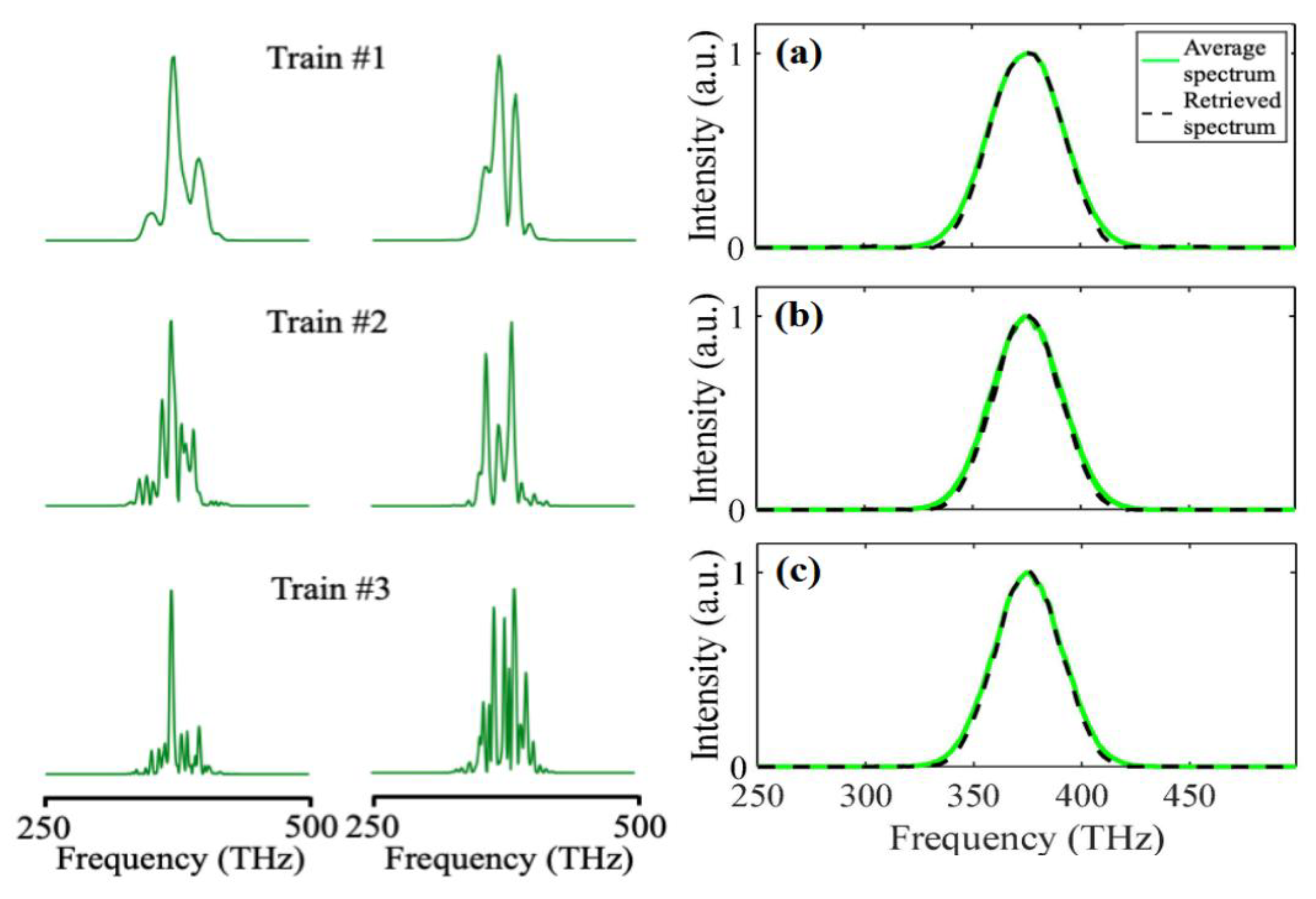

Table 1.
Parameters used to retrieve trains with trace sizes 128 × 128 (26 fs pulse train), 256 × 256 (54 fs pulse train), and 512 × 512 (108 fs pulse train). The abbreviation IG in the table indicates “initial guess”.
Table 1.
Parameters used to retrieve trains with trace sizes 128 × 128 (26 fs pulse train), 256 × 256 (54 fs pulse train), and 512 × 512 (108 fs pulse train). The abbreviation IG in the table indicates “initial guess”.
| N | # of IGs N/4×N/4 array (RANA) | # of iterations N/4×N/4 array (RANA) | # of IGs N/2×N/2 array (RANA) | # of iterations N/2×N/2 array (RANA) | # of IGs N×N array (RANA) | Minimum G’ error |
|---|---|---|---|---|---|---|
| 128 | 20 | 40 | 12 | 35 | 4 | ~0.2 |
| 256 | 32 | 40 | 16 | 35 | 4 | ~0.3 |
| 512 | 48 | 55 | 24 | 45 | 4 | ~0.4 |
Table 2.
The average G’ errors in 100 retrievals using the GP algorithm and RANA approach from noisy PG/TG FROG traces and the TBPrms of all the retrieved fields. Note that the G’ errors and TBPs for RANA tend to be consistently less than those for the standard GP algorithm.
Table 2.
The average G’ errors in 100 retrievals using the GP algorithm and RANA approach from noisy PG/TG FROG traces and the TBPrms of all the retrieved fields. Note that the G’ errors and TBPs for RANA tend to be consistently less than those for the standard GP algorithm.
| G′, GP | G′, RANA | TBP, GP | TBP, RANA | |
|---|---|---|---|---|
| Train #1 | 0.188 ± 0.005 | 0.182 ± 0.003 | 1.79 ± 0.07 | 1.80 ± 0.08 |
| Train #2 | 0.311 ± 0.027 | 0.289 ± 0.006 | 5.51 ± 0.43 | 5.28 ± 0.28 |
| Train #3 | 0.443 ± 0.048 | 0.377 ± 0.009 | 12.6 ± 1.4 | 10.4 ± 0.7 |
Disclaimer/Publisher’s Note: The statements, opinions and data contained in all publications are solely those of the individual author(s) and contributor(s) and not of MDPI and/or the editor(s). MDPI and/or the editor(s) disclaim responsibility for any injury to people or property resulting from any ideas, methods, instructions or products referred to in the content. |
© 2025 by the authors. Licensee MDPI, Basel, Switzerland. This article is an open access article distributed under the terms and conditions of the Creative Commons Attribution (CC BY) license (http://creativecommons.org/licenses/by/4.0/).
Copyright: This open access article is published under a Creative Commons CC BY 4.0 license, which permit the free download, distribution, and reuse, provided that the author and preprint are cited in any reuse.


