Submitted:
13 October 2025
Posted:
16 October 2025
You are already at the latest version
Abstract
Deep learning, as a multifaceted computational framework, integrates function approximation, optimization, and statistical learning within a rigorously formulated mathematical landscape. This work systematically develops the theoretical foundations of deep learning through functional analysis, measure theory, and variational calculus, establishing a mathematically exhaustive treatment of deep learning paradigms. We begin with a rigorous problem formulation by defining the risk functional as a mapping between measurable function spaces, analyzing its properties via Fr´echet differentiability and convex functional minimization. The complexity of deep neural networks is examined using VC-dimension theory and Rademacher complexity, characterizing generalization bounds and hypothesis class constraints. The universal approximation properties of neural networks are refined through convolution operators, the Stone-Weierstrass theorem, and Sobolev embeddings, with quantifiable expressivity bounds derived using Fourier analysis and compactness arguments via the Rellich-Kondrachov theorem. The expressivity trade-offs between depth and width are analyzed through capacity measures, spectral representations of activation functions, and energy-based functional approximations. The mathematical structure of training dynamics is developed by rigorously studying gradient flow, stationary points, and Hessian eigenspectrum properties of loss landscapes. The Neural Tangent Kernel (NTK) regime is formalized as an asymptotic linearization of deep learning dynamics, with precise spectral decomposition methods providing theoretical insights into generalization. Generalization bounds are established using PAC-Bayesian techniques, spectral regularization, and information-theoretic constraints, elucidating the stability of deep networks under probabilistic risk formulations. The study extends to advanced deep learning architectures, including convolutional neural networks (CNNs), recurrent neural networks (RNNs), transformers, generative adversarial networks (GANs), and variational autoencoders (VAEs), with rigorous functional analysis of their representational capacities. Optimal transport theory is explored in deep learning through Wasserstein distances, Sinkhorn regularization, and Kantorovich duality, connecting generative modeling to probability space embeddings. Theoretical formulations of game-theoretic deep learning architectures are examined, establishing variational inequalities, equilibrium constraints, and evolutionary stability conditions in adversarial learning paradigms. Reinforcement learning is formalized through stochastic control theory, Bellman operators, and dynamic programming principles, with rigorous derivations of policy optimization strategies. We provide an advanced treatment of optimization techniques, including stochastic gradient descent (SGD), adaptive moment estimation (Adam), and Hessian-based second-order methods, with a focus on spectral regularization and convergence guarantees. The role of information-theoretic constraints in deep learning generalization is further analyzed through rate-distortion theory, entropy-based priors, and variational inference techniques. Metric learning, adversarial robustness, and Bayesian deep learning are rigorously formulated, with explicit derivations of Mahalanobis distances, Gaussian mixture models, extreme value theory, and Bayesian nonparametric priors. Few-shot and zero-shot learning paradigms are examined through meta-learning frameworks, Model-Agnostic Meta-Learning (MAML), and Bayesian hierarchical inference. The mathematical structure of neural network architecture search (NAS) is developed using evolutionary algorithms, reinforcement learning-based policy optimization, and differential operator constraints. Theoretical advancements in kernel regression, deep Kolmogorov methods, and neural approximations of differential operators are rigorously examined, connecting deep learning models to functional approximation in infinite-dimensional Hilbert spaces. The mathematical principles underlying causal inference in deep learning are formulated through structural causal models (SCMs), counterfactual reasoning, domain adaptation, and invariant risk minimization. Deep learning frameworks are analyzed through the lens of variational functionals, tensor calculus, and high-dimensional probability theory. This work presents a mathematically exhaustive, rigorously formulated, and scientifically rigorous synthesis of deep learning theory, bridging fundamental mathematical principles with cutting-edge advancements in neural network research. By unifying functional analysis, information theory, stochastic processes, and optimization into a cohesive theoretical framework, this study serves as a definitive reference for researchers seeking to extend the mathematical foundations of deep learning.
Keywords:
Deep Learning
; Neural Networks
; Universal Approximation Theorem
; Risk Functional
; Measurable Function Spaces
; VC-Dimension
; Rademacher Complexity
; Sobolev Embeddings
; Rellich-Kondrachov Theorem
; Gradient Flow
; Hessian Structure
; Neural Tangent Kernel (NTK)
; PAC-Bayes Theory
; Spectral Regularization
; Fourier Analysis in Deep Learning
; Convolutional Neural Networks (CNNs)
; Recurrent Neural Networks (RNNs)
; Transformers and Attention Mechanisms
; Generative Adversarial Networks (GANs)
; Variational Autoencoders (VAEs)
; Reinforcement Learning
; Stochastic Gradient Descent (SGD)
; Adaptive Optimization (Adam
; RMSProp)
; Function Space Approximation
; Generalization Bounds
; Mathematical Foundations of AI
1. Mathematical Foundations
Deep learning is an algorithmic framework for addressing high-dimensional function approximation tasks. Fundamentally, it is based on the synergy of:
- Functional Approximation: Modeling complex, non-linear functions with neural networks. Functional approximation is one of the building blocks of deep learning, and it lies at the core of how deep learning models, especially neural networks, are able to tackle hard problems. In deep learning, functional approximation means the capability of neural networks to approximate complex, high-dimensional, and non-linear functions that tend to be hard or impossible to model with standard mathematical methods.
- Optimization Theory: Efficiently solving non-convex optimization problems. Optimization theory is a key area of deep learning, as training deep neural networks is really just minimizing the best set of parameters (weights and biases) of a given objective, commonly referred to as the loss function. The objective will usually be some measure of difference between the network outputs and the actual values. Optimization methods control the process of training and decide the extent to which a neural network may learn from data.
- Statistical Learning Theory: Generalization behavior on unseen data. Statistical Learning Theory (SLT) gives the mathematical basis for the generalization behavior of machine learning methods, including deep learning methods. It provides important insights into how models generalize from training data to novel data, and this is very important in making sure that deep learning models are not just correct on the training set but also work well on new, unseen data. SLT assists in solving basic issues like overfitting, bias-variance tradeoff, and generalization error.
The problem can be formalized as:
where X is the input space, Y is the output space, P is the distribution of data, is a loss function, are neural network parameters. This problem entails the integration of various fields, each of which is examined in systematic detail below.
1.1. Problem Definition: Risk Functional as a Mapping Between Spaces
1.1.1. Measurable Function Spaces
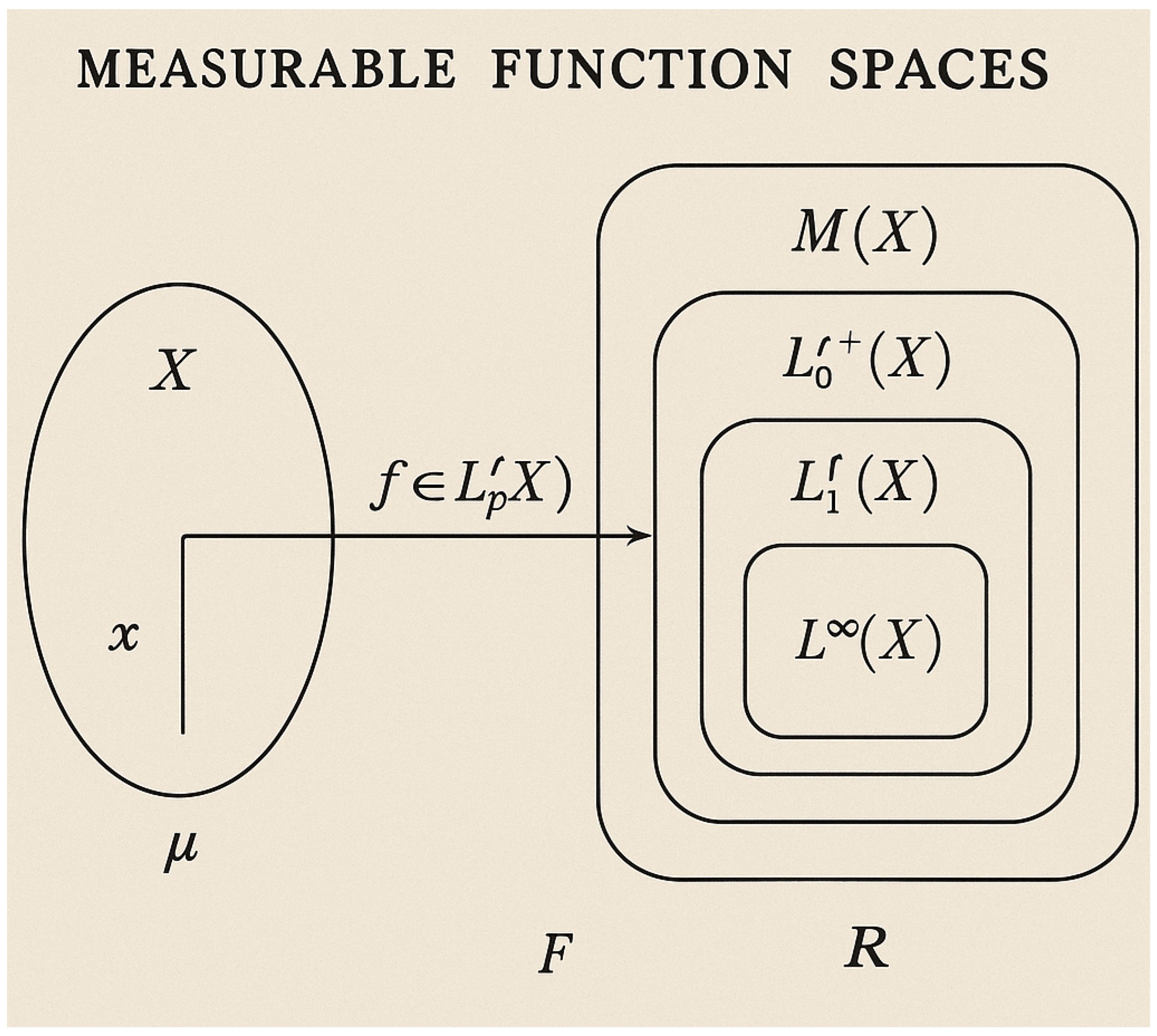
A measurable space is the basic building block of measure theory, notated as , in which is an arbitrary but fixed non-empty set called the sample space or underlying set and is a -algebra, that is, a particular class of subsets of capturing the measurability notion. The -algebra , the power set of , holds three axioms, each guaranteeing an essential property of closure with respect to set operations. To start with, is closed under complementation such that for every set , the complement is also in . This ensures the possibility of establishing the "non-occurrence" of measurable events in a mathematically coherent manner. Second, is closed under countable unions: for any countable family , the union is also in , allowing measurable sets to be constructed out of countably infinite operations. De Morgan’s laws subsequently suggest countable intersection closure, since , so that the structure supports conjunctions of countable sets of events. Lastly, the presence of the empty set is an axiom which allows for a null reference point, so that the -algebra is not empty and can be used to express the "impossibility" of some outcomes.
Figure 1.
Measurable Function Spaces
1.1.1.1 Literature Review of Measurable Function Spaces
Rao et. al. (2024) [1] investigated approximation theory within Lebesgue measurable function spaces, providing an analysis of operator convergence. They also established a theoretical framework for function approximation in Lebesgue spaces and provided a rigorous study of symmetric properties in function spaces. Mukhopadhyay and Ray (2025) [2] provided a comprehensive introduction to measurable function spaces, with a focus on Lp-spaces and their completeness properties. They also established the fundamental role of Lp-spaces in measure theory and discussed the relationship between continuous function spaces and measurable functions. Szołdra (2024) [3] examined measurable function spaces in quantum mechanics, exploring the role of measurable observables in ergodic theory. They connected functional analysis and measure theory to quantum state evolution and provided a mathematical foundation for quantum machine learning in function spaces. Lee (2025) [10] investigated metric space theory and functional analysis in the context of measurable function spaces in AI models. He formalized how function spaces can model self-referential structures in AI and provided a bridge between measure theory and generative models. Song et. al. (2025) [4] discussed measurable function spaces in the context of urban renewal and performance evaluation. They developed a rigorous evaluation metric using measurable function spaces and explored function space properties in applied data science and urban analytics. Mennaoui et. al. (2025) [5] explored measurable function spaces in the theory of evolution equations, a key concept in functional analysis. They established a rigorous study of measurable operator functions and provided new insights into function spaces and their role in solving differential equations. Pedroza (2024) [6] investigated domain stability in machine learning models using function spaces. He established a formal mathematical relationship between function smoothness and domain adaptation and uses topological and measurable function spaces to analyze stability conditions in learning models. Cerreia-Vioglio and Ok (2024) [7] developed a new integration theory for measurable set-valued functions. They introduced a generalization of integration over Banach-valued functions and established weak compactness properties in measurable function spaces. Averin (2024) [8] applied measurable function spaces to gravitational entropy theory. He provided a rigorous proof of entropy bounds using function space formalism and connected measure theory with relativistic field equations. Potter (2025) [9] investigated measurable function spaces in the context of Fourier analysis and crystallographic structures. He established new results on Fourier transforms of measurable functions and introduced a novel framework for studying function spaces in invariant shift operators.
1.1.1.2 Analysis of Measurable Function Spaces
Measurable spaces are not merely abstract structures but are the backbone of measure theory, probability, and integration. For example, the Borel -algebra on the real numbers is the smallest -algebra containing all open intervals for . This -algebra is pivotal in defining Lebesgue measure, where measurable sets generalize the classical notion of intervals to include sets that are neither open nor closed. Moreover, the construction of a -algebra generated by a collection of subsets , denoted , provides a minimal framework that includes and satisfies all -algebra properties, enabling the systematic extension of measurability to more complex scenarios. For instance, starting with intervals in , one can build the Borel -algebra, a critical tool in modern analysis.
The structure of a measurable space allows the definition of a measure , a function that assigns a non-negative value to each set in , adhering to two key axioms: and countable additivity, which states that for any disjoint collection , the measure of their union satisfies . This property is indispensable in extending intuitive notions of length, area, and volume to arbitrary measurable sets, paving the way for the Lebesgue integral. A function is then termed -measurable if for every Borel set , the preimage belongs to . This definition ensures that the function is compatible with the -algebra, a necessity for defining integrals and expectation in probability theory.
In summary, measurable spaces represent a highly versatile and mathematically rigorous framework, underpinning vast areas of analysis and probability. Their theoretical depth lies in their ability to systematically handle infinite operations while maintaining closure, consistency, and flexibility for defining measures, measurable functions, and integrals. As such, the rigorous study of measurable spaces is indispensable for advancing modern mathematical theory, providing a bridge between abstract set theory and applications in real-world phenomena.
Let and be measurable spaces. The true risk functional is defined as:
where:
- f belongs to a hypothesis space .
- is a Borel probability measure over , satisfying .
1.1.2. Risk as a Functional
1.1.2.1 Literature Review of Risk as a Functional
Wang et. al. (2025) [11] developed a mathematical risk model based on functional variational calculus and introduced a loss functional regularization framework that minimizes adversarial risk in deep learning models. They also proposed a game-theoretic interpretation of functional risk in security settings. Duim and Mesquita (2025) [12] extended the inverse reinforcement learning (IRL) framework by defining risk as a functional over probability spaces and used Bayesian functional priors to model risk-sensitive behavior. They also introduced an iterative regularized risk functional minimization approach. Khayat et. al. (2025) [13] established functional Sobolev norms to quantify risk in adversarial settings and introduced a functional risk decomposition technique using deep neural architectures. They also provided an in-depth theoretical framework for risk estimation in adversarially perturbed networks. Agrawal (2025) [14] developed a variational framework for risk as a loss functional and used adaptive weighting of loss functions to enhance generalization in deep learning. He also provided rigorous convergence analysis of risk functional minimization. Hailemichael and Ayalew (2025) [15] used control barrier function (CBF) theory to develop risk-aware deep learning models and modeled risk as a functional on dynamical systems, optimizing stability and robustness. They also introduced a risk-minimizing constrained optimization formulation. Nguyen et.al. (2025) [16] developed a functional metric learning approach for risk-sensitive deep models and used convex optimization techniques to derive functional risk bounds. They also established semi-supervised loss functions for risk-regularized learning. Luo et. al. (2025) [17] introduced a geometric interpretation of risk functionals in deep learning models and used integral transform techniques to approximate risk in real-world vision systems. They also developed a functional approach to adversarial robustness.
1.1.2.2 Analysis of Risk as a Functional
The functional is Fréchet-differentiable if:
where denotes the inner product in . In the field of risk management and decision theory, the concept of a risk functional is a mathematical formalization that captures how risk is quantified for a given outcome or state. A risk functional, denoted as , acts as a map that takes elements from a given space X (which represents the possible outcomes or states) and returns a real-valued risk measure. This risk measure, , expresses the degree of risk or the adverse outcome associated with a particular element . The space X may vary depending on the context—this could be a space of random variables, trajectories, or more complex function spaces. The risk functional maps x to , i.e., , where each reflects the risk associated with the specific realization x. One of the most foundational forms of risk functionals is based on the expectation of a loss function , where represents a random variable or state, and quantifies the loss associated with that state. The risk functional can be expressed as an expected loss, written mathematically as:
where is the probability density function of the outcome x, and the integration is taken over the entire space X. In this setup, can be any function that measures the severity or unfavorable nature of the outcome x. In a financial context, could represent the loss function for a portfolio, and would be the probability density function of the portfolio’s returns. In many cases, a specific form of is used, such as , where is the target or expected value. This choice results in the risk functional representing the variance of the outcome x, expressed as:
This formulation captures the variability or dispersion of outcomes around a mean value, a common risk measure in applications like portfolio optimization or risk management. Additionally, another widely used class of risk functionals arises from quantile-based risk measures, such as Value-at-Risk (VaR), which focuses on the extreme tail behavior of the loss distribution. The VaR at a confidence level is defined as the smallest value l such that the probability of exceeding l is no greater than , i.e.,
This defines a threshold beyond which the worst outcomes are expected to occur with probability . Value-at-Risk provides a measure of the worst-case loss under normal circumstances, but it does not provide information about the severity of losses exceeding this threshold. To address this limitation, the Conditional Value-at-Risk (CVaR) is introduced, which measures the expected loss given that the loss exceeds the VaR threshold. Mathematically, CVaR at the level is given by:
This conditional expectation provides a more detailed assessment of the potential extreme losses beyond the VaR threshold. The CVaR is a more comprehensive measure, capturing the tail risk and providing valuable information about the magnitude of extreme adverse events. In cases where the space X represents trajectories or paths, such as in the context of continuous-time processes or dynamical systems, the risk functional is often formulated in terms of integrals over time. For example, consider as a trajectory in the function space , the space of continuous functions on the interval . The risk functional in this case might quantify the total deviation of the trajectory from a reference or target trajectory over time. A typical example could be the total squared deviation, written as:
where represents a reference trajectory and is a norm, such as the Euclidean norm. This risk functional quantifies the total deviation (or energy) of the trajectory from the target path over the entire time interval, and is used in various applications such as control theory and optimal trajectory planning. A common choice for the norm might be , where are the components of the trajectory in . In some cases, the space X of possible outcomes may not be a finite-dimensional vector space, but instead a Banach space or a Hilbert space, particularly when x represents a more complex object such as a function or a trajectory. For example, the space is a Banach space, and the risk functional may involve the evaluation of integrals over this function space. In such settings, the risk functional can take the form:
where is the p-norm, and . For , this risk functional represents the total energy of the trajectory, but other norms can be used to emphasize different types of risks. For instance, the -norm would focus on the maximum deviation of the trajectory from the target path. The concept of convexity plays a significant role in the theory of risk functionals. Convexity ensures that the risk associated with a convex combination of two states and is less than or equal to the weighted average of the risks of the individual states. Mathematically, for , convexity demands that:
This property reflects the diversification effect in risk management, where mixing several states or outcomes generally leads to a reduction in overall risk. Convex risk functionals are particularly important in portfolio theory, where they allow for risk minimization through diversification. For example, if represents the variance of a portfolio’s returns, then the convexity property ensures that combining different assets will result in a portfolio with lower overall risk than the risk of any individual asset. Monotonicity is another important property for risk functionals, ensuring that the risk increases as the outcome becomes more adverse. If is worse than according to some partial order, we have:
Monotonicity ensures that the risk functional behaves in a way that aligns with intuitive notions of risk: worse outcomes are associated with higher risk. In financial contexts, this is reflected in the fact that losses increase the associated risk measure. Finally, in some applications, the risk functional is derived from perturbation analysis to study how small changes in parameters affect the overall risk. Consider as a perturbed trajectory, where is a small parameter, and the Fréchet derivative of the risk functional with respect to is given by:
This derivative quantifies the sensitivity of the risk to perturbations in the system and is crucial in the analysis of stability and robustness. Such analyses are essential in areas like stochastic control and optimization, where it is important to understand how small changes in the model’s parameters can influence the risk profile.
Thus, the risk functional is a powerful tool for quantifying and managing uncertainty, and its formulation can be adapted to various settings, from random variables and stochastic processes to continuous trajectories and dynamic systems. The risk functional provides a rigorous mathematical framework for assessing and minimizing risk in complex systems, and its flexibility makes it applicable across a wide range of domains.
1.2. Approximation Spaces for Neural Networks
The neural network hypothesis space is parameterized as:
To analyze its capacity, we rely on:
- VC-dimension theory for discrete hypotheses.
- Rademacher complexity for continuous spaces:where are i.i.d. Rademacher random variables.
1.2.1. VC-Dimension Theory for Discrete Hypotheses
The VC-dimension (Vapnik-Chervonenkis dimension) is a fundamental concept in statistical learning theory that quantifies the capacity of a hypothesis class to fit a range of labelings of a set of data points. The VC-dimension is particularly useful in understanding the generalization ability of a classifier. The theory is important in machine learning, especially when assessing overfitting and the risk of model complexity.
1.2.1.1 Literature Review of VC-Dimension Theory for Discrete Hypotheses
There are several articles that explore the VC-dimension theory for discrete hypotheses very rigorously. N. Bousquet and S. Thomassé (2015) [18] explored in their paper the VC-dimension in the context of graph theory, connecting it to structural properties such as the Erdős-Pósa property. Yıldız and Alpaydin (2009) [19] in their article computed the VC-dimension for decision tree hypothesis spaces, considering both discrete and continuous features. Zhang et. al. (2012) [20] introduced a discretized VC-dimension to bridge real-valued and discrete hypothesis spaces, offering new theoretical tools for complexity analysis. Riondato and Zdonik (2011) [21] adapted VC-dimension theory to database systems, analyzing SQL query selectivity using a theoretical lens. Riggle and Sonderegger (2010) [22] investigated the VC-dimension in linguistic models, focusing on grammar hypothesis spaces. Anderson (2023) [23] provided a comprehensive review of VC-dimension in fuzzy systems, particularly in logic frameworks involving discrete structures. Fox et. al. (2021) [24] proved key conjectures for systems with bounded VC-dimension, offering insights into combinatorial implications. Johnson (2021) [25] discusses binary representations and VC-dimensions, with implications for discrete hypothesis modeling. Janzing (2018) [26] in his paper focuses on hypothesis classes with low VC-dimension in causal inference frameworks. Ghosh (2024) [907] derived the expressions for fundamental differential operators—namely the gradient, divergence, and curl—as well as the vector gradient of a vector field within curvilinear coordinate systems. This work significantly enhances clarity on the application of the del operator in non-Cartesian contexts, laying a robust foundation for advanced analytical and computational treatments of vector calculus in complex geometries. Hüllermeier and Tehrani (2012) [27] in their paper explored the theoretical VC-dimension of Choquet integrals, applied to discrete machine learning models. The book titled “Foundations of Machine Learning" [28] by Mehryar Mohri, Afshin Rostamizadeh, and Ameet Talwalkar offers a very good foundational discussion on VC-dimension in the context of statistical learning. Another book titled “Learning Theory: An Approximation Theory Viewpoint" by Felipe Cucker and Ding-Xuan Zhou [29] discusses the role of VC-dimension in approximation theory. Yet another book titled “Understanding Machine Learning: From Theory to Algorithms" by Shai Shalev-Shwartz and Shai Ben-David [30] contains detailed chapters on hypothesis spaces and VC-dimension.
1.2.1.2 Analysis of VC-Dimension Theory for Discrete Hypotheses
For discrete hypotheses, the VC-dimension theory applies to a class of hypotheses that map a set of input points to binary output labels (typically 0 or 1). The VC-dimension for a hypothesis class refers to the largest set of data points that can be shattered by that class, where "shattering" means that the hypothesis class can realize all possible labelings of these points.
We shall now discuss the Formal Mathematical Framework. Let X be a finite or infinite set called the instance space, which represents the input space. Consider a hypothesis class H, where each hypothesis is a function . The function h classifies each element of X into one of two classes: 0 or 1. Given a subset
we say that H shatters S if for every possible labeling , there exists some such that for all , we have:
In other words, a hypothesis class H shatters S if it can produce every possible binary labeling on the set S. The VC-dimension is defined as the size of the largest set S that can be shattered by H:
If no set of points can be shattered, then the VC-dimension is 0. Some Properties of the VC-Dimension are
- Shattering Implies Non-empty Hypothesis Class: If a set S is shattered by H, then H is non-empty. This follows directly from the fact that for each labeling , there exists some that produces the corresponding labeling. Therefore, H must contain at least one hypothesis.
- Upper Bound on Shattering: Given a hypothesis class H, if there exists a set of size k such that H can shatter S, then any set of size greater than k cannot be shattered. This gives us the crucial result that:
- Implication for Generalization A central result in the theory of statistical learning is the connection between VC-dimension and the generalization error. Specifically, the VC-dimension bounds the ability of a hypothesis class to generalize to unseen data. The higher the VC-dimension, the more complex the hypothesis class, and the more likely it is to overfit the training data, leading to poor generalization.
We shall now discuss the VC-Dimension and Generalization Bounds (VC Theorem). The VC-dimension theorem (often referred to as Hoeffding’s bound or the generalization bound) provides a probabilistic guarantee on the relationship between the training error and the true error. Specifically, it gives an upper bound on the probability that the generalization error exceeds the empirical error (training error) by more than .
The Vapnik-Chervonenkis (VC) dimension is a fundamental measure of the capacity of a hypothesis class , and it plays a crucial role in understanding the generalization ability of machine learning models, including neural networks. The VC-dimension of a hypothesis class is defined as the largest number m such that there exists a set of m points that can be shattered by . Formally, a set
is shattered by if for every possible binary labeling , there exists a hypothesis such that
The VC-dimension, denoted as , is the supremum of all such m that can be shattered by . For a neural network with W total parameters (weights and biases), the capacity of the hypothesis class induced by the network architecture depends on the activation function. If the activation function is piecewise linear (such as ReLU), then an upper bound for the VC-dimension is given by
This result is derived from combinatorial arguments involving the number of hyperplane arrangements that a neural network can realize in a given input space.
If the activation function is nonlinear (such as sigmoid or tanh), the capacity can increase but remains constrained by the number of parameters. The intuition behind this bound lies in the observation that each neuron introduces a decision boundary in the input space, and the number of such boundaries grows approximately as rather than W due to dependencies among neurons. When considering discrete hypotheses, the hypothesis space is restricted to a finite number of functions. This occurs in scenarios where the weights and biases are quantized to a finite set of values, or where the activation functions themselves take on a finite number of distinct outputs. If there are K possible distinct values for each parameter and there are W parameters, then the total number of possible functions that the network can realize is at most
From the fundamental relationship between the VC-dimension and the number of hypotheses in a finite hypothesis space, we obtain the bound
Applying this result to a neural network with quantized weights and biases, we obtain
Thus, discretization significantly reduces the VC-dimension compared to continuous-valued networks, where the number of hypotheses is effectively infinite due to the continuous range of parameters. For binary networks, where each weight is restricted to two possible values (e.g., ), the bound simplifies further to
Since VC-dimension directly affects the generalization error, its role in neural network theory is formalized through the following uniform convergence bound. If h is chosen from based on an i.i.d. training set of size N, then with probability at least , the true error and the empirical error satisfy the bound
A crucial consequence of this inequality is that for a hypothesis class with a larger VC-dimension, a larger number of training samples is required to achieve the same generalization error. Since discrete neural networks have a lower VC-dimension than their continuous counterparts, they often generalize better given the same training set size, provided the hypothesis class is sufficiently expressive for the problem at hand.
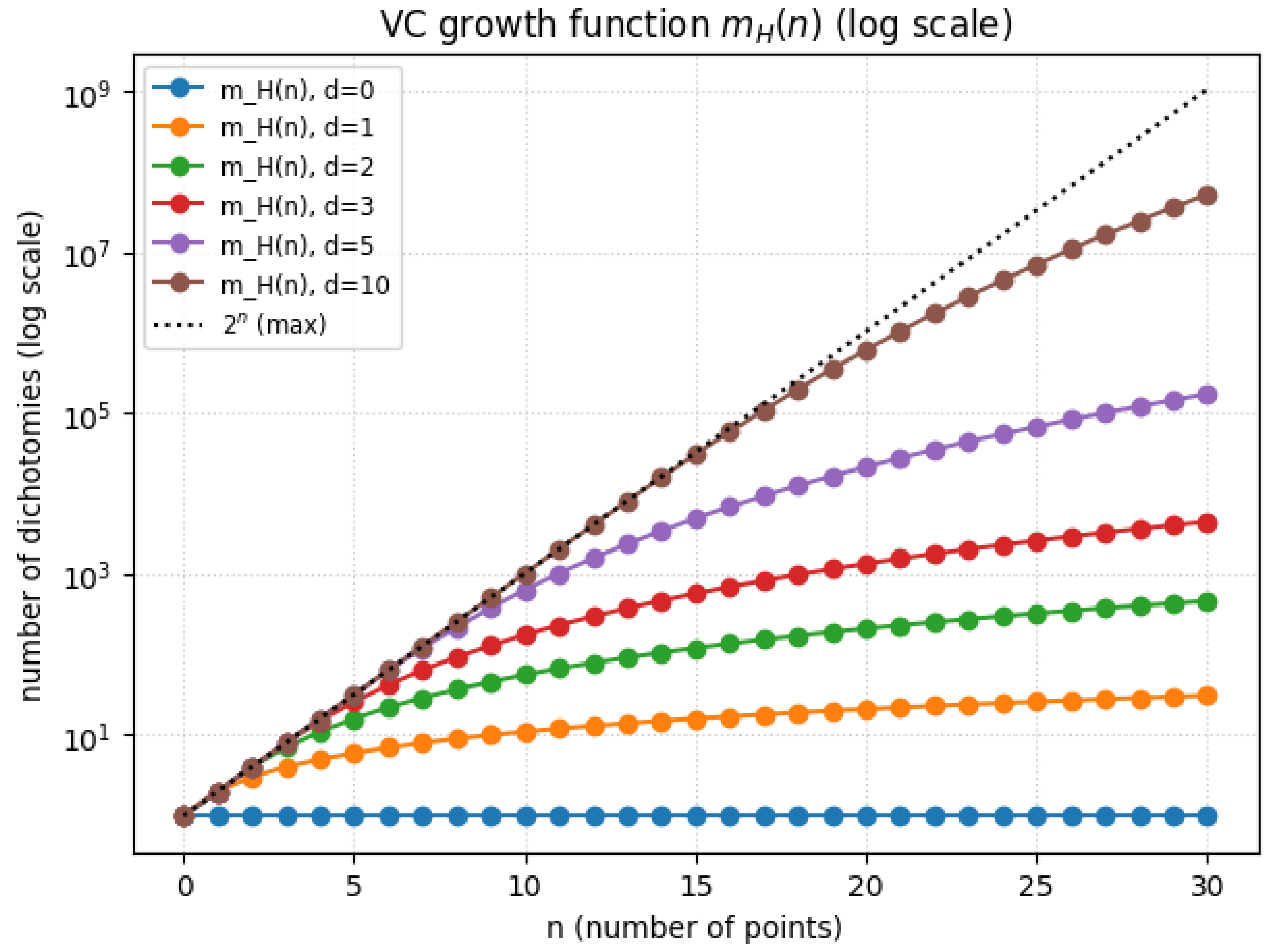
The shattering coefficient, also known as the growth function, plays an essential role in understanding the VC-dimension of neural networks. The shattering coefficient is defined as the maximum number of dichotomies that can realize on any set of m points. If , then can fully shatter an m-point dataset. For neural networks with continuous parameters, the growth function satisfies
For discrete neural networks, where is finite, we obtain the bound
which ensures that the number of realizable functions is significantly smaller than in the continuous case, thereby reducing overfitting potential. The interplay between VC-dimension and structural risk minimization (SRM) further highlights the importance of capacity control in neural networks. Given a hierarchy of hypothesis classes , with increasing VC-dimension, the optimal generalization performance is achieved by choosing the class that minimizes the trade-off between empirical risk and capacity, as given by
For discrete networks, the practical implication of this bound is that models with limited precision weights or constrained architectures tend to generalize better than overparameterized networks with unnecessarily high VC-dimension. From an optimization standpoint, discrete neural networks have a smaller number of local minima in the loss landscape compared to their continuous counterparts. This is because the number of unique parameter configurations is finite, leading to a more structured and potentially more tractable optimization problem. However, the trade-off is that discrete optimization is often NP-hard, requiring specialized techniques such as simulated annealing, evolutionary algorithms, or integer programming methods. Thus, VC-dimension theory provides profound insights into the expressive power, generalization ability, and optimization complexity of neural networks. Discrete neural networks exhibit a reduced VC-dimension compared to their continuous counterparts, leading to potentially better generalization, provided that the model retains sufficient expressivity for the given problem. The trade-off between expressivity and generalization is fundamental to designing efficient neural network architectures that perform well in practice.
Let be the distribution from which the training data is drawn, and let and represent the empirical error and true error of a hypothesis , respectively:
where are i.i.d. (independent and identically distributed) samples from the distribution . For a hypothesis class H with VC-dimension , with probability at least , the following holds for all :
where is bounded by:
This result shows that the generalization error (the difference between the true and empirical error) is small with high probability, provided the sample size n is large enough and the VC-dimension d is not too large. The sample complexity n required to guarantee that the generalization error is within with high probability is given by:
where C is a constant depending on the distribution. This bound emphasizes the importance of VC-dimension in controlling the complexity of the hypothesis class. A larger VC-dimension requires a larger sample size to avoid overfitting and ensure reliable generalization. Some Detailed Examples are:
- Example 1: Linear Classifiers in : Consider the hypothesis class H consisting of linear classifiers in . These classifiers are hyperplanes in two dimensions, defined by:where is the weight vector and is the bias term. The VC-dimension of linear classifiers in is 3. This can be rigorously shown by noting that for any set of 3 points in , the hypothesis class H can shatter these points. In fact, any possible binary labeling of the 3 points can be achieved by some linear classifier. However, for 4 points in , it is impossible to shatter all possible binary labelings (e.g., the four vertices of a convex quadrilateral), meaning the VC-dimension is 3.
- Example 2: Polynomial Classifiers of Degree d: Consider a polynomial hypothesis class in of degree d. The hypothesis class H consists of polynomials of the form:where the are coefficients and . The VC-dimension of polynomial classifiers of degree d in grows as , implying that the complexity of the hypothesis class increases rapidly with both the degree d and the dimension n of the input space.
Neural networks, depending on their architecture, can have very high VC-dimensions. In particular, the VC-dimension of a neural network with L layers, each containing N neurons, is typically , indicating that the VC-dimension grows exponentially with both the number of neurons and the number of layers. This result provides insight into the complexity of neural networks and their capacity to overfit data when the training sample size is insufficient.
The VC-dimension of a hypothesis class is a powerful tool in statistical learning theory. It quantifies the complexity of the hypothesis class by measuring its capacity to shatter sets of points, and it is directly tied to the model’s ability to generalize. The VC-dimension theorem provides rigorous bounds on the generalization error and sample complexity, giving us essential insights into the trade-off between model complexity and generalization. The theory extends to more complex hypothesis classes such as linear classifiers, polynomial classifiers, and neural networks, where it serves as a critical tool for controlling overfitting and ensuring reliable performance on unseen data.
1.2.1.3 Python Code to Generate Figure 2 and Figure 3 Illustrating VC-Dimension Theory for Discrete Hypotheses
The Python code below produces the Figure 2 and Figure 3 illustrating VC-dimension theory for discrete hypotheses.
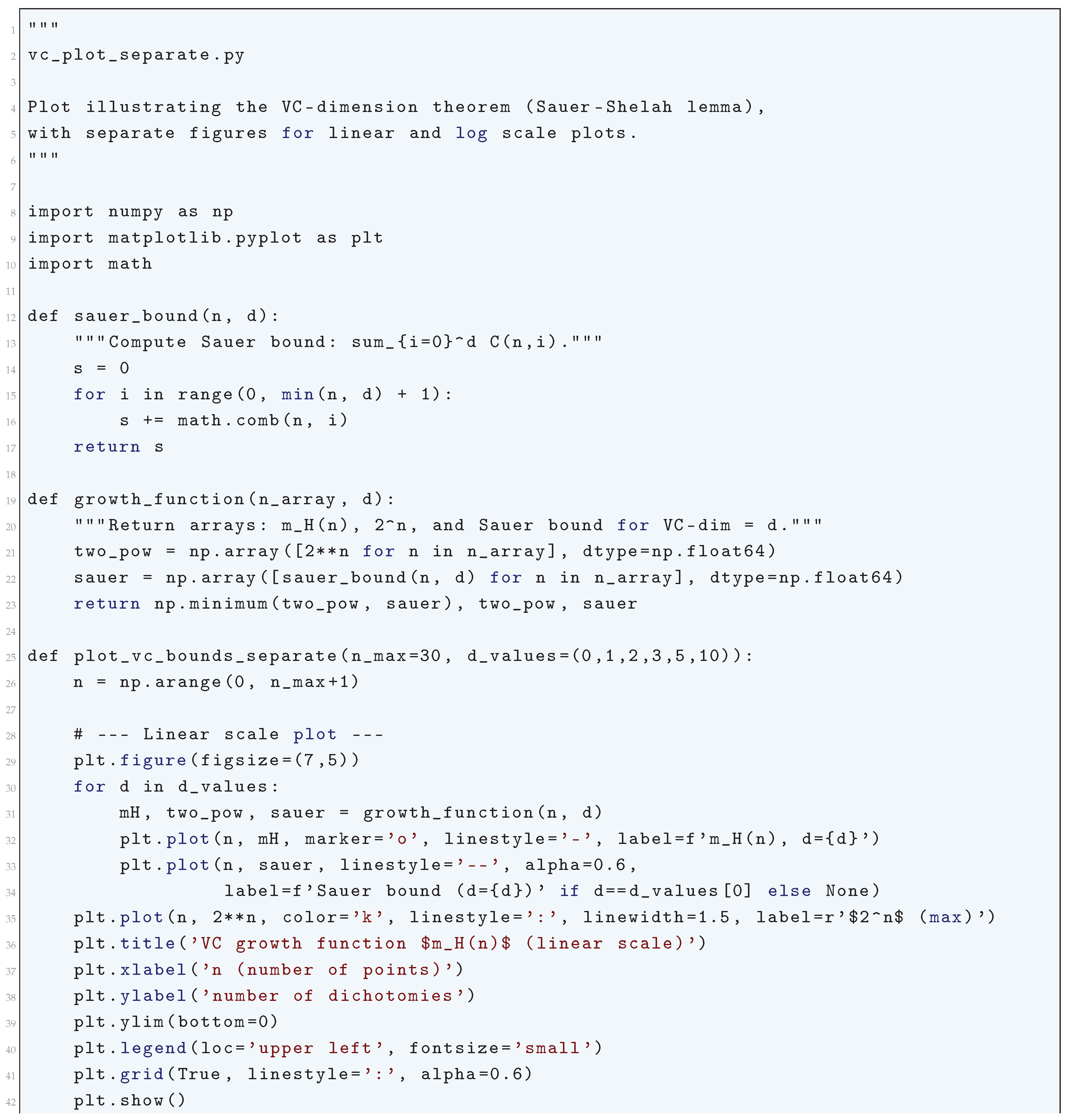
Figure 2.
VC growth function (Linear scale)
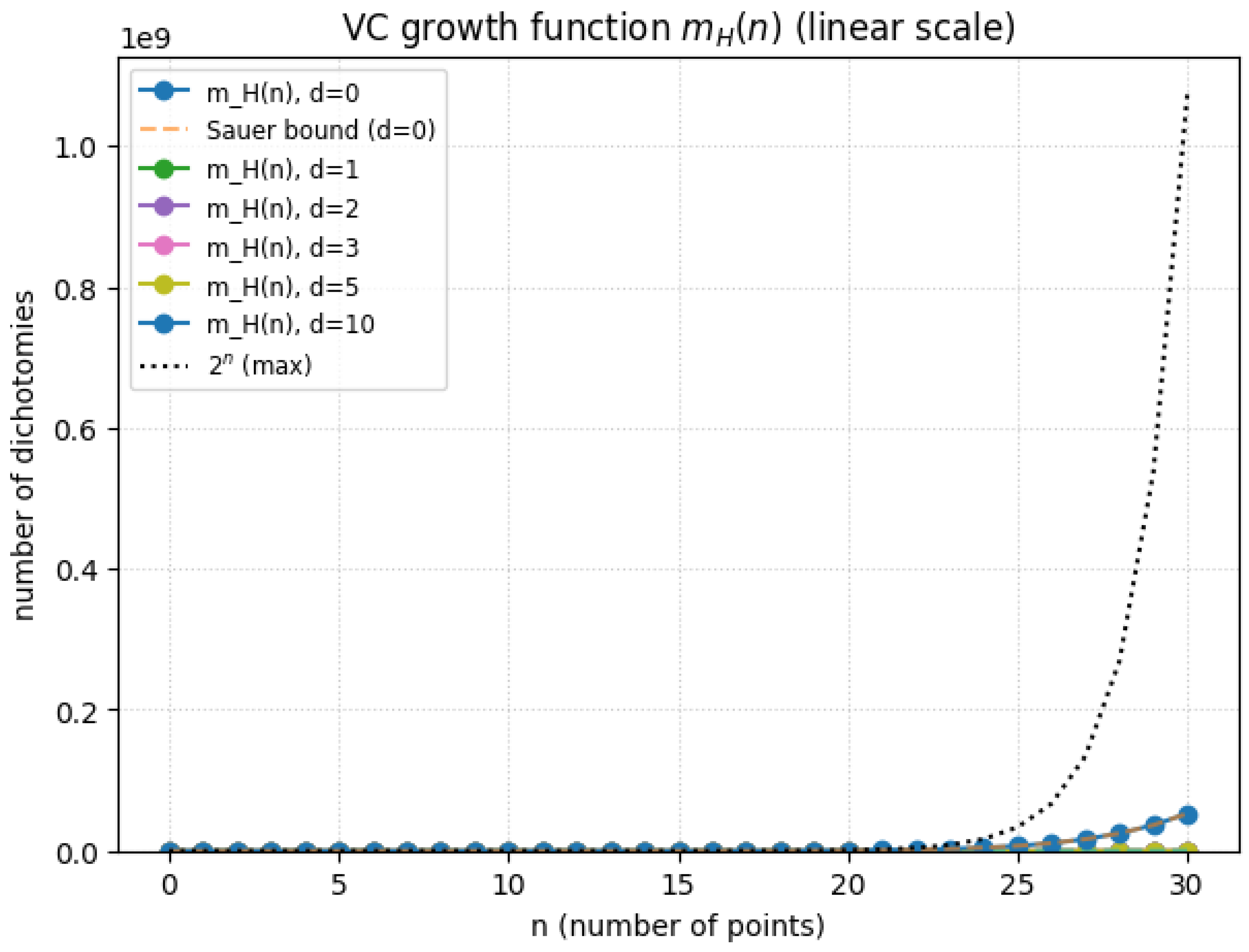
Figure 3.
VC growth function (Log scale)
1.2.2. Rademacher Complexity for Continuous Spaces
1.2.2.1 Literature Review of Rademacher Complexity for Continuous Spaces
Truong (2022) [31] in his article explored how Rademacher complexity impacts generalization error in deep learning, particularly with IID and Markov datasets. Gnecco and Sanguineti (2008) [32] developed approximation error bounds in Reproducing Kernel Hilbert Spaces (RKHS) and functional approximation settings. Astashkin (2010) [33] discusses applications of Rademacher functions in symmetric function spaces and their mathematical structure. Ying and Campbell (2010) [34] applies Rademacher complexity to kernel-based learning problems and support vector machines. Zhu et.al. (2009) [35] examined Rademacher complexity in cognitive models and neural representation learning. Astashkin et al. (2020) [36] investigated how the Rademacher system behaves in function spaces and its role in functional analysis. Sachs et.al. (2023) [37] introduced a refined approach to Rademacher complexity tailored to specific machine learning algorithms. Ma and Wang (2020) [38] investigated Rademacher complexity bounds in deep residual networks. Bartlett and Mendelson (2002) [39] wrote a foundational paper on complexity measures, providing fundamental theoretical insights into generalization bounds. Dzahini and Wild (2024) [40] in their paper extended Rademacher-based complexity to stochastic optimization methods. McDonald and Shalizi (2011) [41] showed using sequential Rademacher complexities for I.I.D process how to control the generalization error of time series models wherein past values of the outcome are used to predict future values.
1.2.2.2 Analysis of Rademacher Complexity for Continuous Spaces
Let represent a probability space where is a measurable space, is a sigma-algebra, and is a probability measure. The function class satisfies:
where denotes the essential supremum. For rigor, is assumed measurable in the sense that for every , there exists a countable subset such that:
Given , the empirical measure is:
The integral under for approximates the population integral under :
Let be independent Rademacher random variables:
These variables are defined on a probability space independent of the sample S.
The Duality and Symmetrization of Empirical Rademacher Complexity is also very important. The empirical Rademacher complexity of with respect to S is:
where denotes expectation over . The supremum can be interpreted as a functional dual norm in , where is the unit ball. Using the symmetrization technique, the Rademacher complexity relates to the deviation of from :
where:
This is derived by first symmetrizing the sample and then invoking Jensen’s inequality and the independence of . There are some Complexity Bounds that use Covering Numbers and Entropy that need to be discussed. In Metric Entropy, we let be the metric on . The covering number satisfies:
Regarding the Dudley’s Entropy Integral, For a bounded function class (compact under ):
There is also a Relation to Talagrand’s Concentration Inequality. Talagrand’s inequality provides tail bounds for the supremum of empirical processes:
reinforcing the link between and generalization.
There are some Applications in Continuous Function Classes. One example is the RKHS with Gaussian Kernel. For as the unit ball of an RKHS with kernel , the covering number satisfies:
yielding:
For , the covering number depends on the smoothness s and dimension d:
Rademacher complexity is deeply embedded in modern empirical process theory. Its intricate relationship with measure-theoretic tools, symmetrization, and concentration inequalities provides a robust theoretical foundation for understanding generalization in high-dimensional spaces.
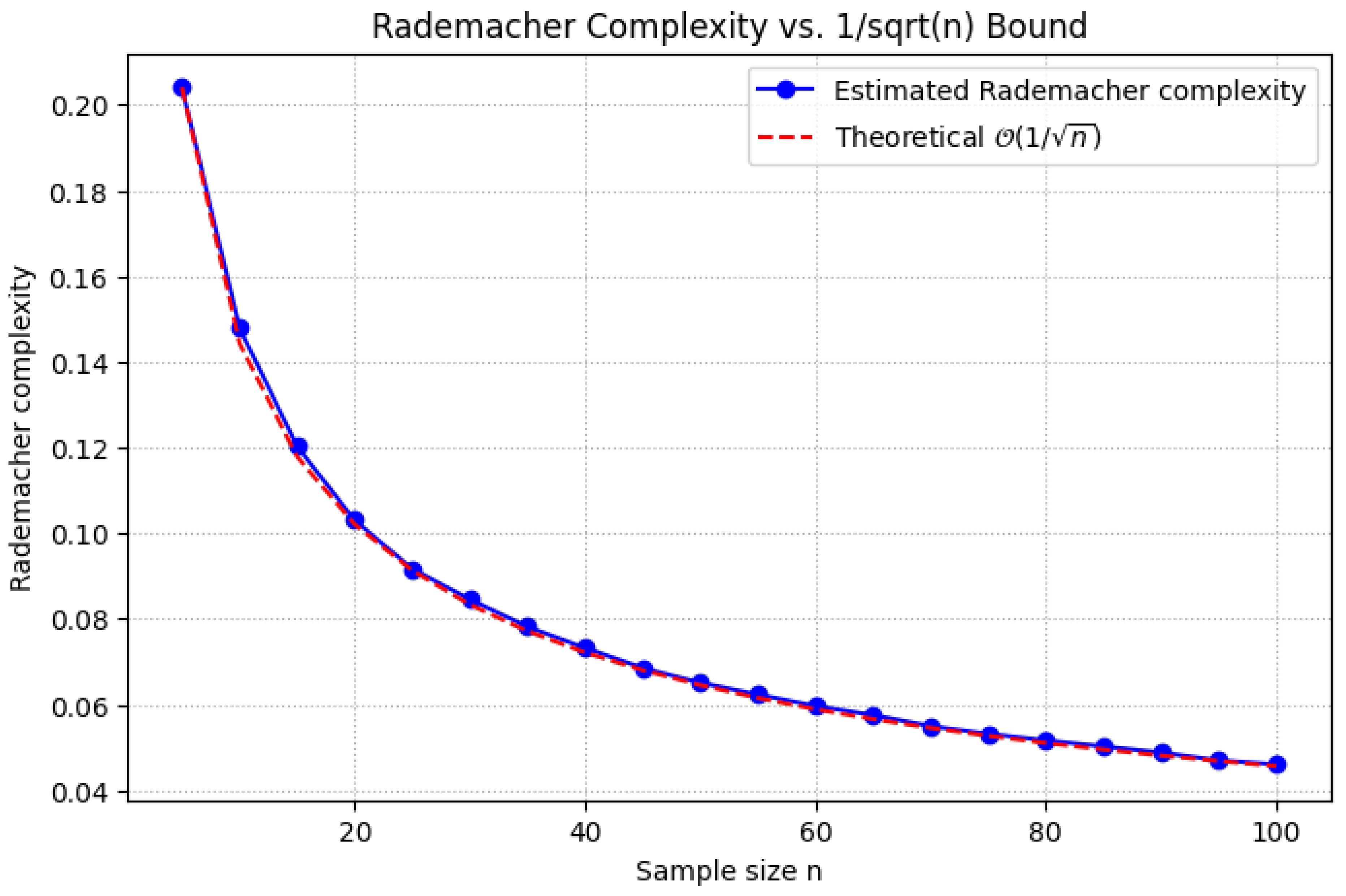
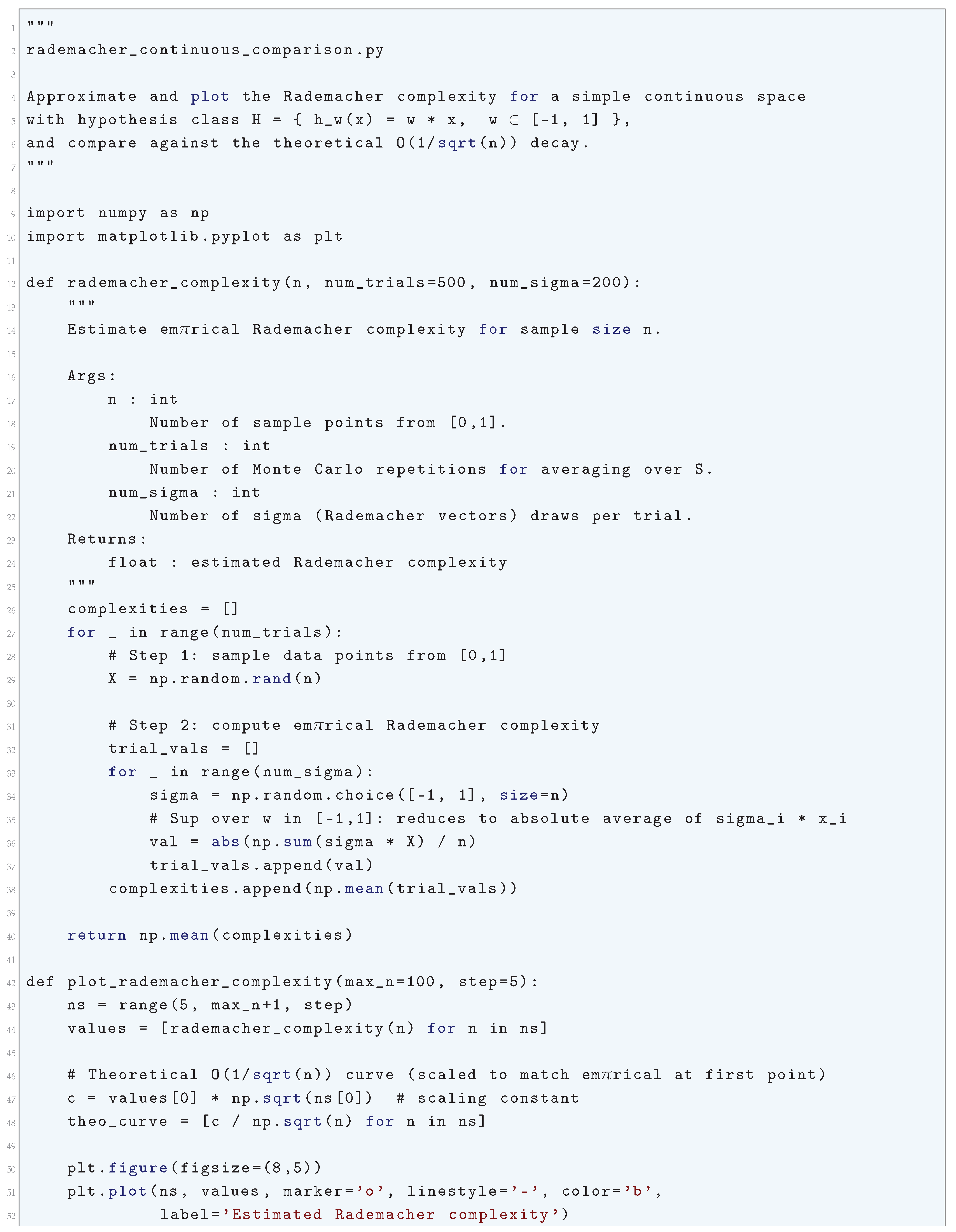
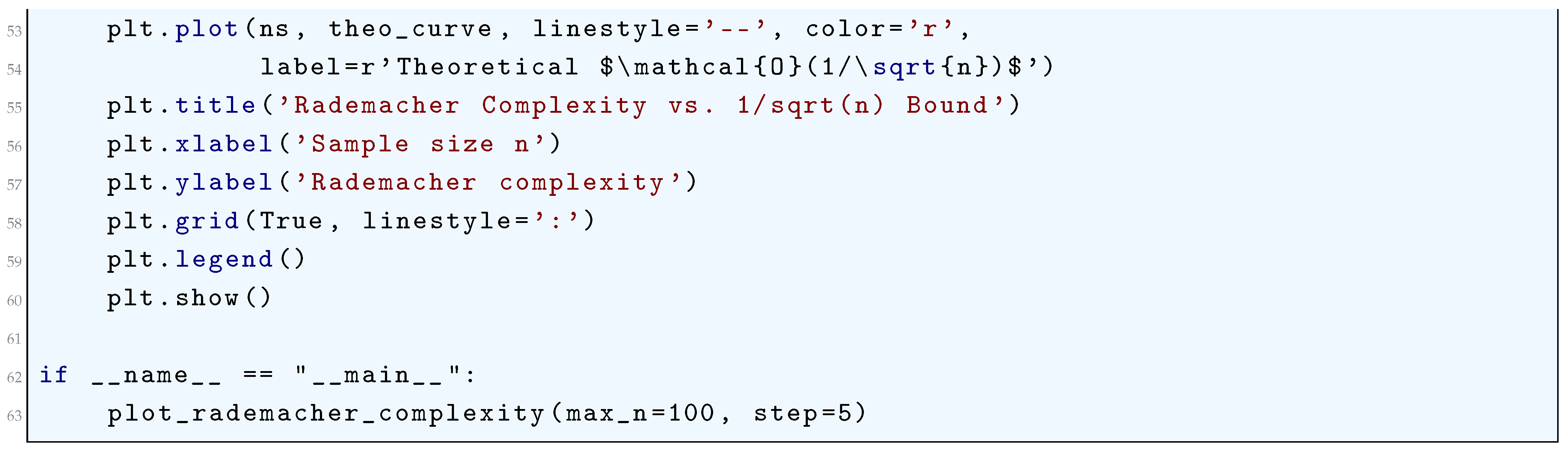
1.2.2.3 Python Code to Generate Figure 4 Illustrating Rademacher Complexity vs. Bound
The Python code below produces the Figure 4 illustrating Rademacher Complexity vs. Bound.
Figure 4.
Rademacher Complexity vs. Bound
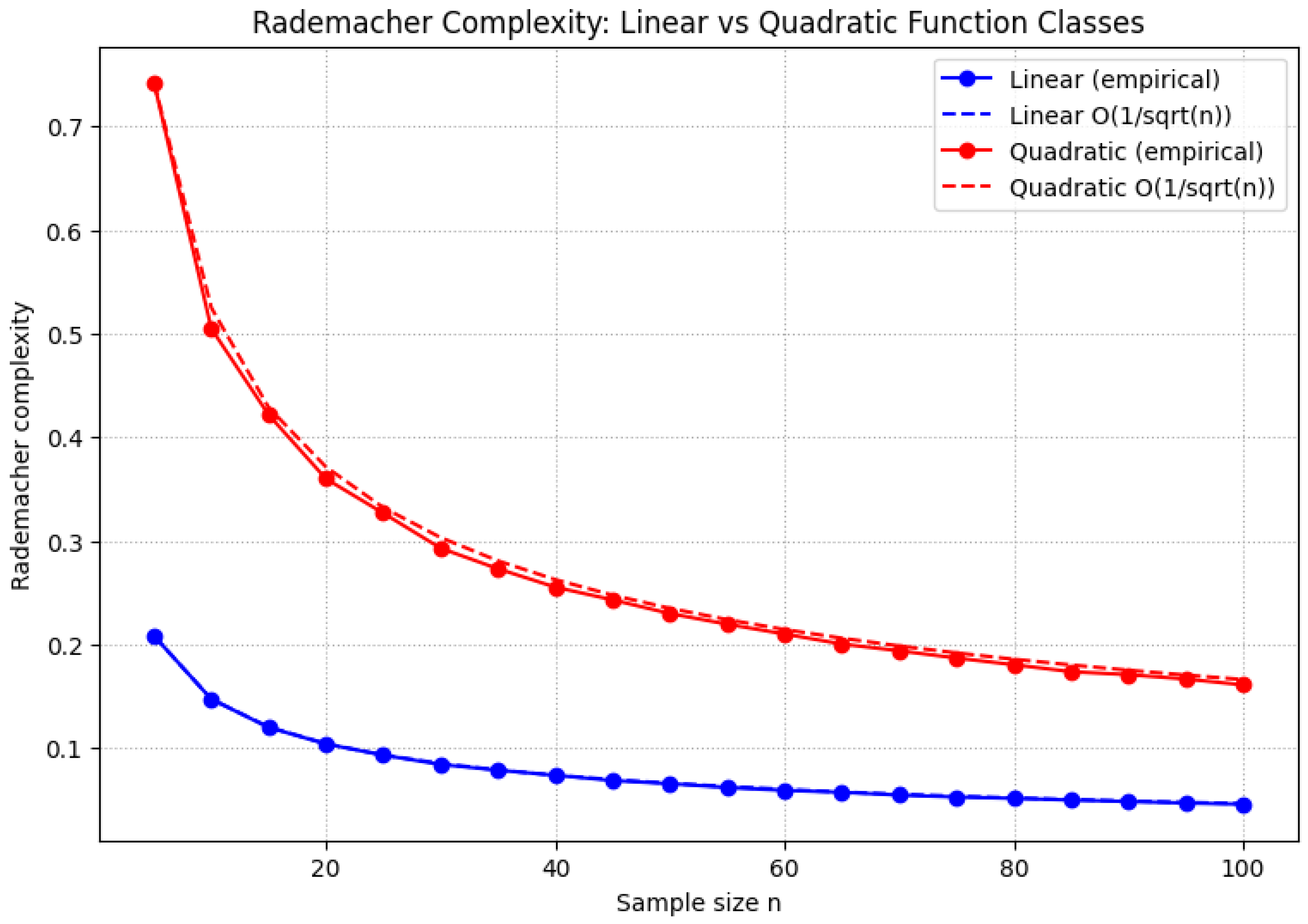
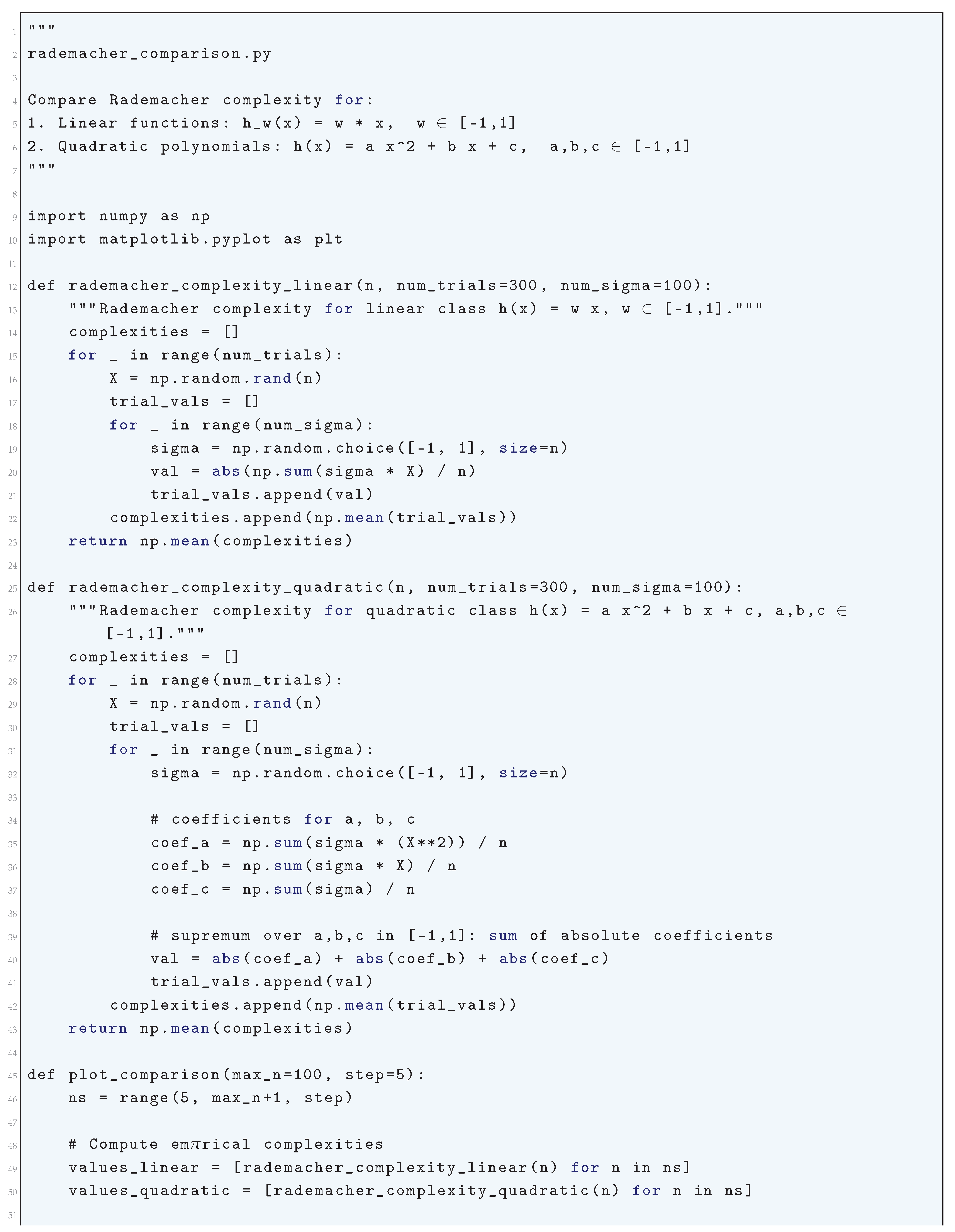
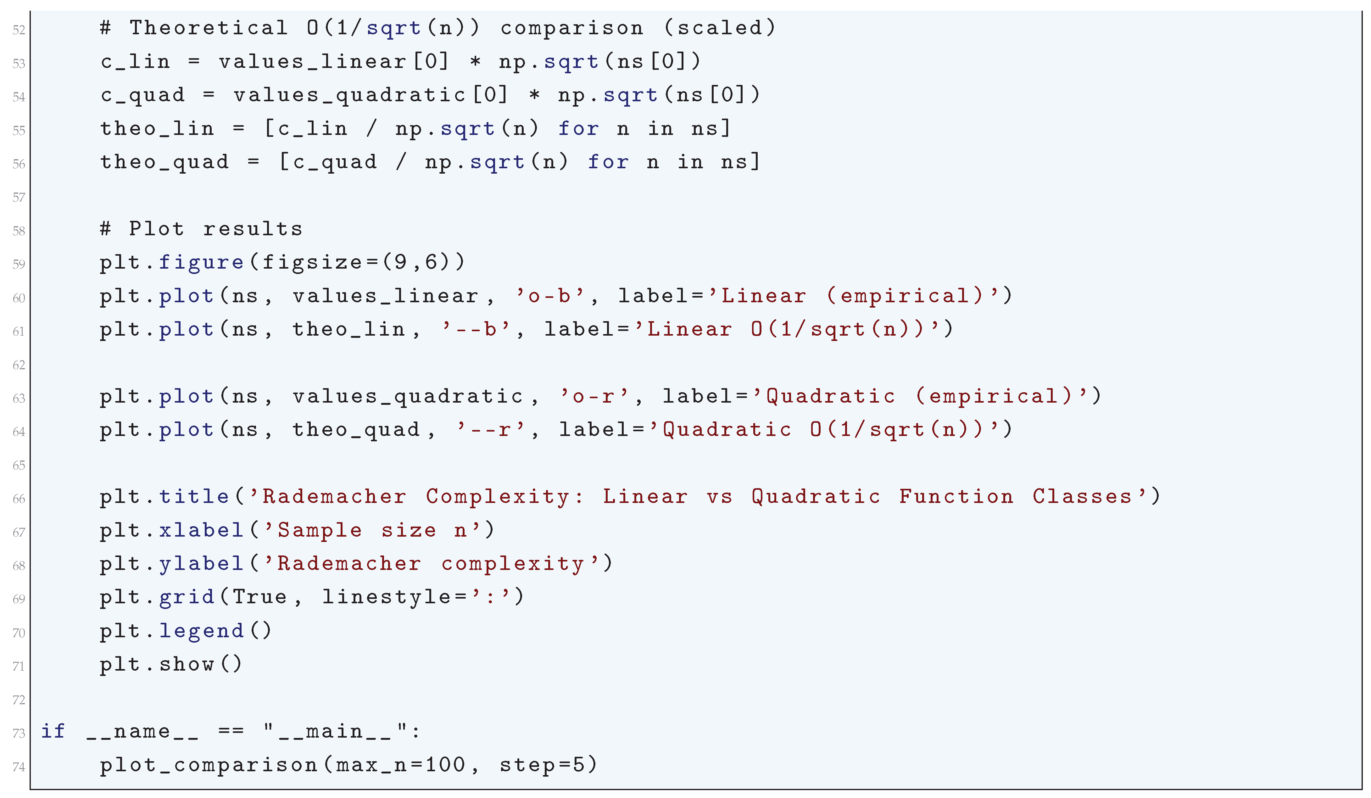
1.2.2.4 Python Code to Generate Figure 5 Illustrating Rademacher Complexity: Linear vs Quadratic Function Classes
The Python code below produces the Figure 5 illustrating Rademacher Complexity: Linear vs Quadratic Function Classes.
Figure 5.
Rademacher Complexity: Linear vs Quadratic Function Classes
1.2.3. Sobolev Embeddings
1.2.3.1 Literature Review of Sobolev Embeddings
Abderachid and Kenza (2024) [42] in their paper investigated fractional Sobolev spaces defined using Riemann-Liouville derivatives and studies their embedding properties. It establishes new continuous embeddings between these fractional spaces and classical Sobolev spaces, providing applications to PDEs. Giang et.al. (2024) [43] introduced weighted Sobolev spaces and derived new Pólya-Szegö type inequalities. These inequalities play a key role in establishing compact embedding results in function spaces equipped with weight functions. Ruiz and Fragkiadaki (2024) [44] provided a novel approach using Haar functions to revisit fractional Sobolev embedding theorems and demonstrated the algebra properties of fractional Sobolev spaces, which are essential in nonlinear analysis. Bilalov et.al. (2025) [45] analyzed compact Sobolev embeddings in Banach function spaces, extending the classical Poincaré and Friedrichs inequalities to this setting and provided applications to function spaces used in modern PDE theory. Cheng and Shao (2025) [46] developed the weighted Sobolev compact embedding theorem for function spaces with unbounded radial potentials and used this result to prove the existence of ground state solutions for fractional Schrödinger-Poisson equations. Wei and Zhang (2025) [47] established a new embedding theorem tailored to variational problems arising in Schrödinger-Poisson equations and used Hardy-Sobolev embeddings to study the zero-mass case, an important case in quantum mechanics. Zhang and Qi (2025) [48] examined the compactness of Sobolev embeddings in the presence of small perturbations in quasilinear elliptic equations and proved multiple solution existence results using variational methods. Xiao and Yue (2025) [49] established a Sobolev embedding theorem for fractional Laplacian function spaces and applied the embedding results to image processing, particularly edge detection. Pesce and Portaro (2025) [50] studied intrinsic Hölder spaces and their connection to fractional Sobolev embeddings and established new embedding results for function spaces relevant to ultraparabolic operators.
1.2.3.2 Analysis of Sobolev Embeddings
The Sobolev embedding theorem states that:
if , ensuring for smooth activations . For a function , its weak derivative satisfies:
where is the weak derivative.
This definition extends the classical notion of differentiation to functions that may not be pointwise differentiable. The Sobolev norm encapsulates both function values and their derivatives:
Key properties:
- Semi-norm Dominance: The Wk,p-norm is controlled by the seminorm , ensuring sensitivity to highorder derivatives.
- Poincaré Inequality: For Ω bounded, u − uΩ satisfies:
Sobolev spaces embed into or , depending on and n. These embeddings govern the smoothness and integrability of u and its derivatives. There are several Advanced Theorems on Sobolev Embeddings. They are as follows:
-
Sobolev Embedding Theorem: Let be a bounded domain with Lipschitz boundary. Then:
- If k > n/p, Wk,p(Ω) ↪ Cm,α() with m = ⌊k − n/p⌋ and α = k − n/p − m.
- If k = n/p, Wk,p(Ω) ↪ Lq(Ω) for q < ∞.
- If k < n/p, Wk,p(Ω) ↪ Lq(Ω) where .
-
Rellich-Kondrachov Compactness Theorem: The embedding is compact for . Compactness follows from:
- (a)
- Equicontinuity: -boundedness ensures uniform control over oscillations.
- (b)
- Rellich’s Selection Principle: Strong convergence follows from uniform estimates and tightness.
The Proof of Sobolev Embedding starts with the Scaling Analysis. Define . Then:
For derivatives:
The scaling relation aligns with the Sobolev embedding condition . Sobolev norms in are equivalent to decay rates of Fourier coefficients:
For , Fourier decay implies uniform bounds, ensuring .
Interpolation spaces bridge and , providing finer embeddings. Duality: Sobolev embeddings are equivalent to boundedness of adjoint operators in . For , ensures
if . Sobolev spaces govern variational problems in geometry, e.g., minimal surfaces and harmonic maps. On with fractal boundaries, trace theorems refine Sobolev embeddings.
The Sobolev Embedding Theorem provides a continuous embedding of the space into a Hölder space when the regularity index exceeds the spatial dimension, specifically when . The Hölder exponent is not arbitrary but is given by the precise fractional part of this index. The fundamental equation is
but this holds strictly only if this value is less than 1. The general formulation is
provided . This relation is derived from scaling invariance properties of the underlying Sobolev norms. Consider the dilation . The Sobolev norm scales as
while the Hölder seminorm scales as
For an embedding to be scale-invariant, the scaling exponents must be consistent across the inequality
which forces the condition
leading directly to the identification
The optimality of this exponent is rigorously demonstrated by examining borderline functions that saturate the Sobolev inequalities. A canonical example is the function defined on a bounded domain containing the origin. Its membership in is determined by the integrability of its derivatives. The norm of the k-th derivative involves integrating
In n dimensions, using spherical coordinates, this integral is finite near zero if and only if
which requires , or equivalently, . Conversely, the Hölder continuity of is determined by the ratio . For , this seminorm is finite if and only if . The limiting case shows that a function can be in yet fail to be Hölder continuous for any exponent greater than . This is formalized by considering the function
where a detailed calculation shows that for , the function belongs to only if , but its Hölder seminorm is infinite, proving that the embedding
for the critical exponent , but holds for any .
The quantitative control offered by the Hölder exponent is expressed through the embedding inequality , where the norm on the left is defined as
The constant C depends on , and the domain . The mathematical rigor of the exponent is further highlighted in the Gagliardo-Nirenberg interpolation inequalities, which provide estimates of the form
where the parameters satisfy
and
Setting , , and seeking continuity implies , which recovers the condition . The Hölder exponent emerges when estimating the modulus of continuity directly from the -norm via the integral representation of a function through its derivatives, such as using the Fourier transform or convolution with a mollifier, leading to pointwise estimates like
for , where
For higher derivatives, the general formula
consistently appears, governing the precise degree of classical regularity attainable from weak solutions. This makes the Hölder exponent a fundamental bridge between the measurable, integral-based world of Sobolev spaces and the pointwise, geometric world of classical analysis.
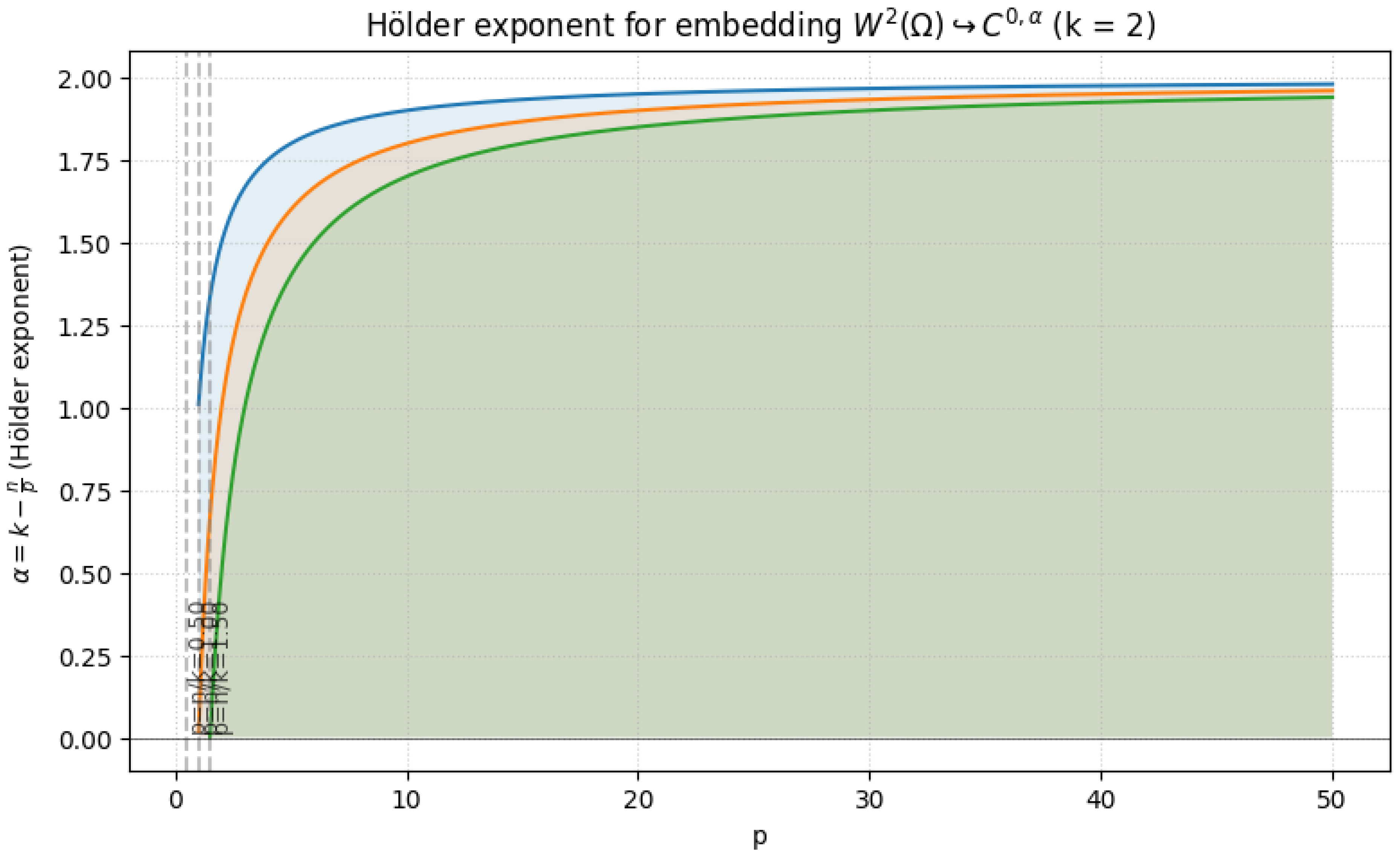
1.2.3.3 Python Code to Generate Figure 6, Figure 7, Figure 8, and Figure 9 Illustrating Sobolev Embeddings
The Python code below produces the Figure 6, Figure 7, Figure 8, and Figure 9 illustrating Sobolev Embeddings.
Figure 6.
Sobolev conjugate (k = 1)
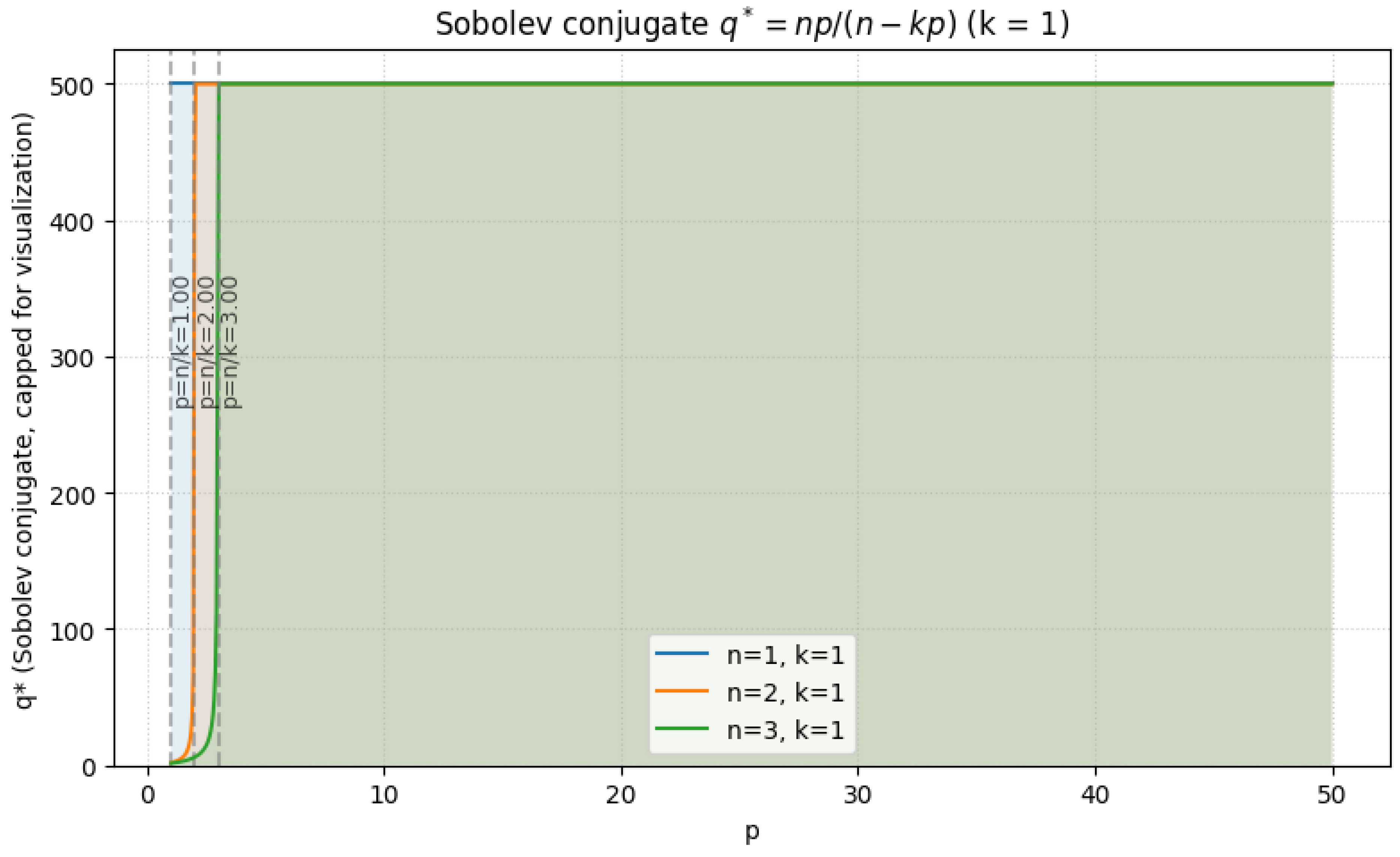
Figure 7.
Sobolev conjugate (k = 2)
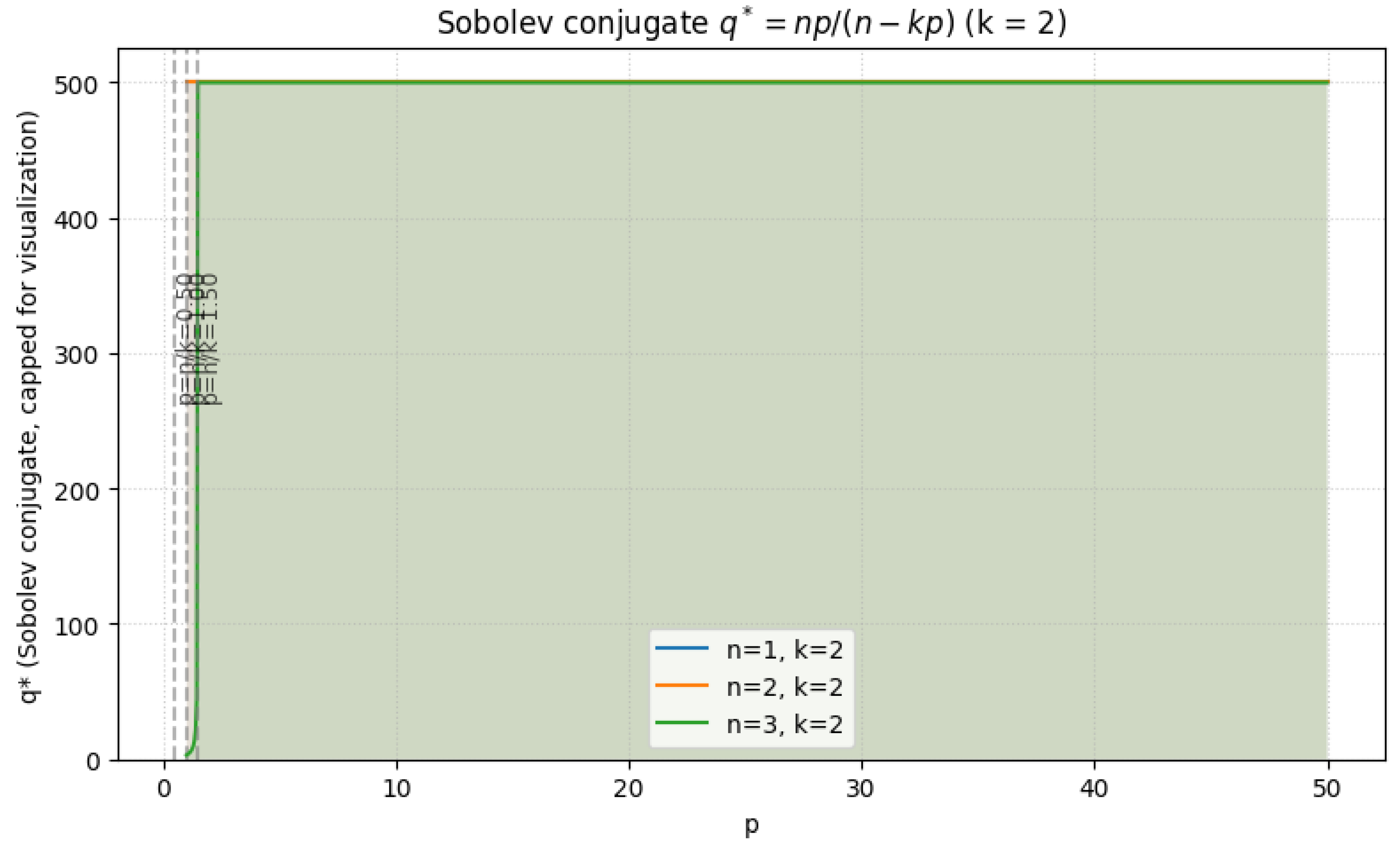
Figure 8.
Hölder exponent for embedding
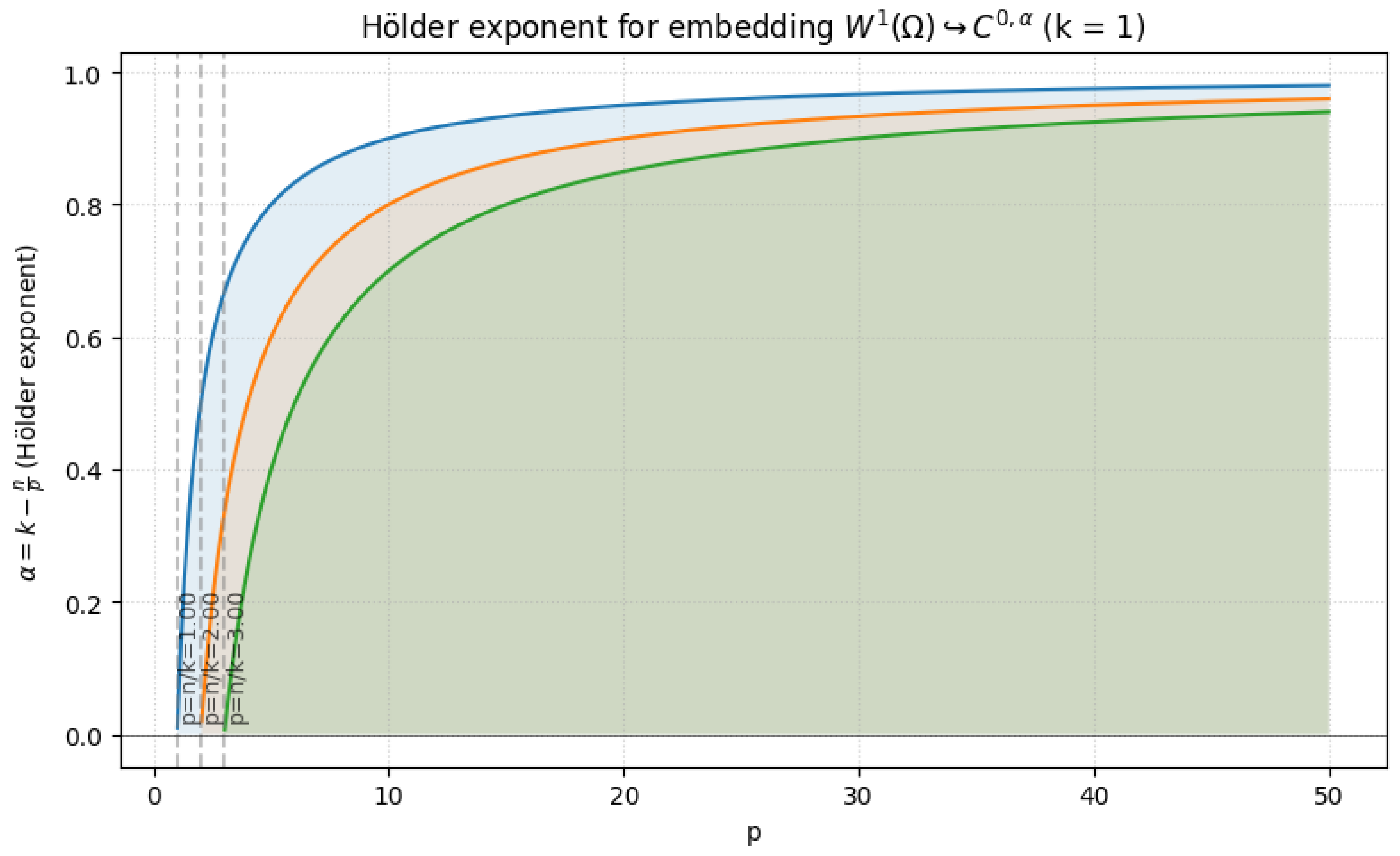
Figure 9.
Hölder exponent for embedding
1.2.4. Rellich-Kondrachov Compactness Theorem
The Rellich-Kondrachov Compactness Theorem is one of the most fundamental and deep results in the theory of Sobolev spaces, particularly in the study of functional analysis and the theory of partial differential equations. The theorem asserts the compactness of certain Sobolev embeddings under appropriate conditions on the domain and the function spaces involved. This result is of immense significance in mathematical analysis because it provides a rigorous justification for the fact that bounded sequences in Sobolev spaces, under certain conditions, have strongly convergent subsequences in lower-order normed spaces. In essence, the theorem states that while weak convergence in Sobolev spaces is relatively straightforward due to the Banach-Alaoglu theorem, strong convergence is not always guaranteed. However, under the assumptions of the Rellich-Kondrachov theorem, strong convergence in can indeed be obtained from boundedness in . The compactness property ensured by this theorem is much stronger than mere boundedness or weak convergence and plays a crucial role in proving the existence of solutions to variational problems by ensuring that minimizing sequences possess convergent subsequences in an appropriate function space. The theorem can also be viewed as a generalization of the classical Arzelà–Ascoli theorem, extending compactness results to function spaces that involve derivatives.
1.2.4.1 Literature Review of Rellich-Kondrachov Compactness Theorem
Lassoued (2026) [51] examined function spaces on the torus and their lack of compactness, highlighting cases where the classical Rellich-Kondrachov result fails. He extended compact embedding results to function spaces with periodic structures. He also discussed trace theorems and regular function spaces in this new context. Chen et.al. (2024) [52] extended the Rellich-Kondrachov theorem to Hörmander vector fields, a class of differential operators that appear in hypoelliptic PDEs. They established a degenerate compact embedding theorem, generalizing previous results in the field. They also provided applications to geometric inequalities, highlighting the role of compact embeddings in PDE theory. Adams and Fournier (2003) [53] in their book provided a complete proof of the Rellich-Kondrachov theorem, along with a discussion of compact embeddings. They also covered function space theory, embedding theorems, and applications in PDEs. Brezis (2010) [55] wrote a highly recommended resource for understanding Sobolev spaces and their compactness properties. The book included applications to variational methods and weak solutions of PDEs. Evans (2022) [56] in his classic PDE textbook includes a discussion of compact Sobolev embeddings, their implications for weak convergence, and applications in variational methods. Maz’ya (2011) [57] provided a detailed treatment of Sobolev space theory, including compact embedding theorems in various settings.
1.2.4.2 Analysis of Rellich-Kondrachov Compactness Theorem
To rigorously state the theorem, we consider a bounded open domain with a Lipschitz boundary. For , the theorem asserts that the embedding
is compact whenever . More precisely, this means that if is a bounded sequence in the Sobolev norm, i.e., there exists a constant such that
then there exists a subsequence and a function such that
which means that
To establish this rigorously, we first recall the fact that bounded sequences in are weakly precompact. Since is a reflexive Banach space for , the Banach-Alaoglu theorem ensures that any bounded sequence in has a subsequence (still denoted by ) and a function such that
This means that for all test functions , where is the Hölder conjugate of p satisfying , we have
However, weak convergence alone does not imply compactness. To obtain strong convergence in , we need additional arguments.
This is accomplished using the Fréchet-Kolmogorov compactness criterion, which states that a bounded subset of is compact if and only if it is tight and uniformly equicontinuous. More formally, compactness follows if
- The sequence does not oscillate excessively at small scales.
- The sequence does not escape to infinity in a way that prevents strong convergence.
To quantify this, we invoke the Sobolev-Poincaré inequality, which states that for , there exists a constant C such that
Applying this inequality to , we obtain
Since is weakly convergent in , we have
Thus,
which establishes the strong convergence in , completing the proof. The key insight is that compactness arises because the gradients of provide control over the oscillations of , ensuring that the sequence cannot oscillate indefinitely without converging in norm. The crucial role of Sobolev embeddings is to guarantee that even though does not embed compactly into itself, it does embed compactly into for . This embedding ensures that weak convergence in implies strong convergence in , proving the theorem.
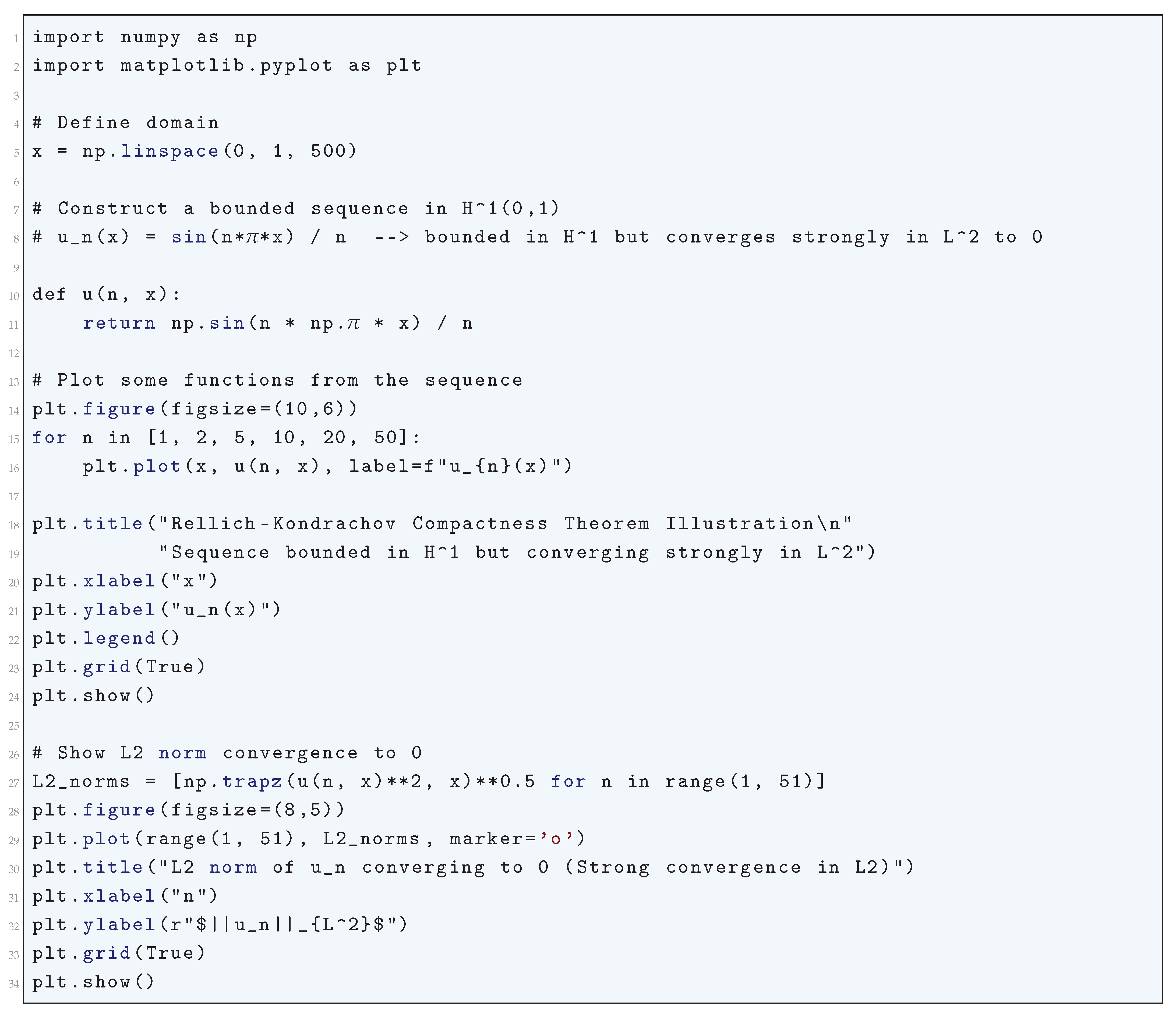
1.2.4.3 Python Code to Generate Figure 10 and Figure 11 Illustrating Rellich-Kondrachov Compactness Theorem
The Python code below produces the Figure 10 and Figure 11 illustrating Rellich-Kondrachov Compactness Theorem.
Figure 10.
Rellich-Kondrachov Compactness Theorem Illustration
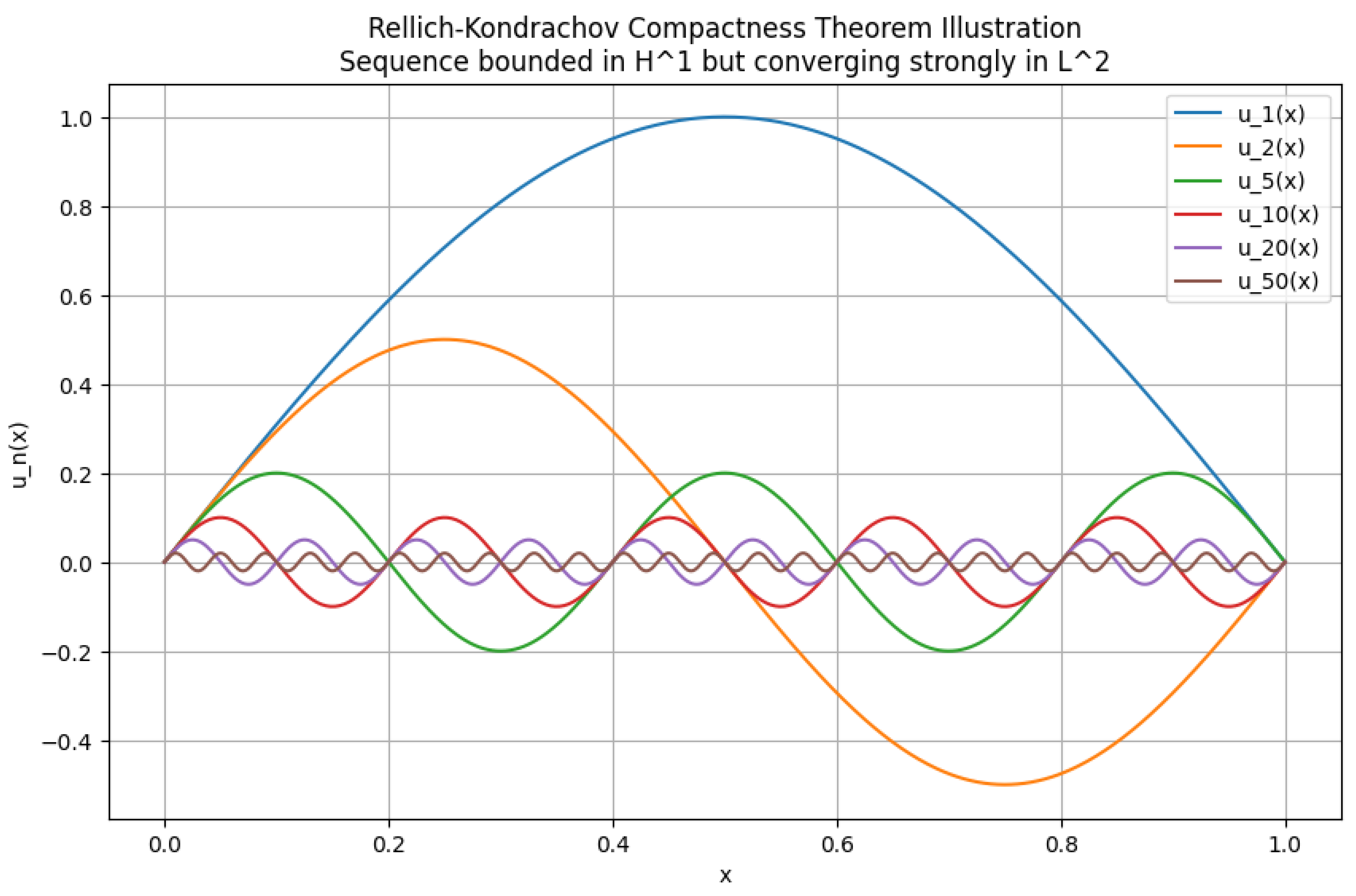
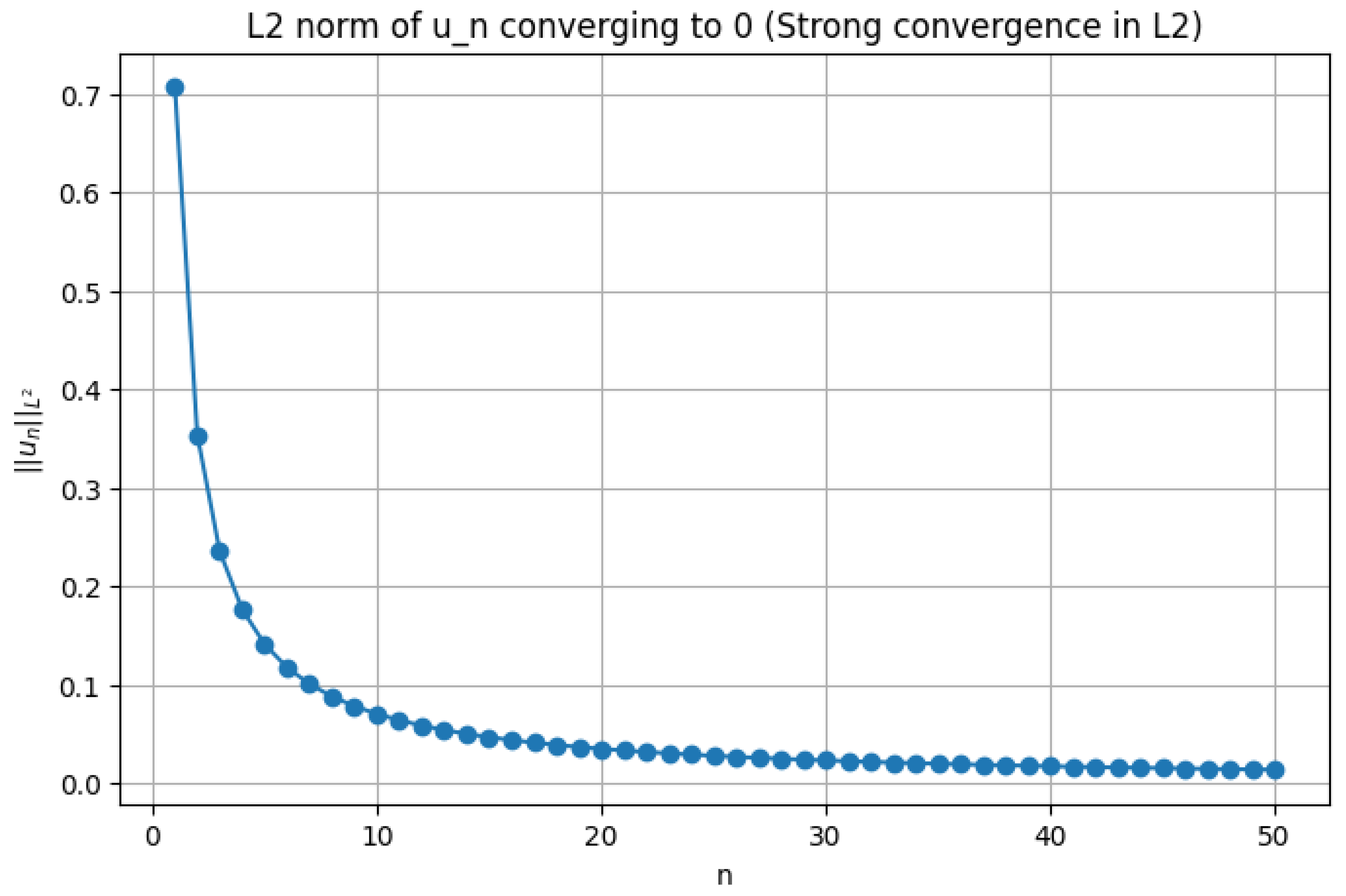
Figure 11.
L2 norm of converging to 0 (Strong convergence in L2)
1.2.5. Fréchet-Kolmogorov Compactness Criterion
1.2.5.1 Literature Review of Fréchet-Kolmogorov Compactness Criterion
The Fréchet-Kolmogorov compactness criterion is a fundamental result in functional analysis, particularly in the study of compact subsets of spaces, and has been extensively discussed and applied in numerous books and articles. One of the most authoritative references is the classic text by Walter Rudin (1973) [70], which provides a rigorous treatment of the criterion, embedding it within the broader context of weak compactness and equicontinuity in spaces. Rudin’s exposition is notable for its clarity and depth, linking the criterion to the Arzelà-Ascoli theorem and emphasizing its utility in proving compactness for families of functions. Another essential reference is by H.L. Royden (1968) [1537], which offers a detailed proof of the Fréchet-Kolmogorov theorem, highlighting its reliance on uniform integrability and tightness conditions. Royden’s treatment is particularly valuable for its pedagogical approach, making the criterion accessible to students while maintaining mathematical rigor. The monograph by Robert A. Adams and John J.F. Fournier (2003) [1522] delves into the Fréchet-Kolmogorov criterion in the context of Sobolev embeddings, demonstrating its critical role in establishing compactness for bounded subsets of Sobolev spaces. Adams and Fournier’s work is indispensable for researchers in partial differential equations, as it connects the criterion to applications in variational methods and elliptic regularity theory. Similarly, by Lawrence C. Evans (2010) [1528] discusses the criterion within the framework of weak convergence and compact embeddings, showcasing its importance in the analysis of solutions to PDEs. Evans’ presentation is particularly rigorous, with a focus on the interplay between the criterion and the Rellich-Kondrachov theorem. Another key text is by Lawrence C. Evans and Ronald F. Gariepy (1992) [1529], which explores the criterion’s implications for functions of bounded variation and its applications in geometric measure theory.
In the realm of probability theory, by Aad W. van der Vaart and Jon A. Wellner (1996) [1540] examines the Fréchet-Kolmogorov criterion as a tool for establishing tightness of probability measures on function spaces. This work is foundational for researchers in empirical process theory, providing a bridge between functional analysis and statistical applications. The authors rigorously develop the criterion’s connection to Prokhorov’s theorem and its use in proving Donsker-type results. Another probabilistic perspective is offered by Patrick Billingsley (1968) [1524], which discusses the criterion in the context of compactness for stochastic processes. Billingsley’s treatment is highly detailed, with a focus on the criterion’s role in proving relative compactness for sequences of measures on metric spaces. For a historical perspective, the original works by Maurice Fréchet (1906) [1541] and Andrey Kolmogorov (1931) [1542] are invaluable. Fréchet’s early 20th-century papers laid the groundwork for the abstract formulation of compactness in function spaces, while Kolmogorov’s contributions refined the criterion, particularly for spaces. These foundational texts are often cited in modern treatments for their pioneering insights. More recently, by Fernando Albiac and Nigel J. Kalton (2006) [1523] provides a modern exposition of the Fréchet-Kolmogorov criterion, embedding it within the broader theory of Banach spaces. Albiac and Kalton’s discussion is notable for its emphasis on the criterion’s relationship with other compactness principles, such as the Eberlein-Šmulian theorem.
The article by Jürgen Appell and Petr P. Zabrejko (1990) [1543] surveys various compactness criteria, including the Fréchet-Kolmogorov theorem, and discusses their applications in nonlinear analysis. This work is particularly useful for its comprehensive overview and its focus on practical implications for integral operators and fixed-point theorems. Another significant contribution is by Klaus Deimling (1985) [1527], which explores the criterion’s use in proving existence theorems for differential equations. Deimling’s treatment is rigorous and application-oriented, making it a valuable resource for researchers in nonlinear analysis. In the context of harmonic analysis, by Gerald B. Folland (1992) [1530] discusses the Fréchet-Kolmogorov criterion in relation to compactness for families of oscillatory integrals. Folland’s exposition is clear and concise, with a focus on the criterion’s role in proving convergence theorems for Fourier series and transforms. Similarly, by Loukas Grafakos (2008) [1531] includes a detailed discussion of the criterion, particularly its applications in the study of singular integrals and maximal functions. Grafakos’ work is highly technical but provides deep insights into the criterion’s utility in modern harmonic analysis.
The Fréchet-Kolmogorov criterion has also been extensively studied in the context of dynamical systems and ergodic theory. By Karl Petersen (1983) [1536] discusses the criterion’s role in proving compactness for families of invariant measures, highlighting its importance in the study of dynamical systems. Petersen’s treatment is mathematically rigorous and includes applications to symbolic dynamics and entropy theory. Another relevant reference is by Anatole Katok and Boris Hasselblatt (1995) [1533], which explores the criterion’s use in establishing compactness for sequences of diffeomorphisms and its implications for structural stability. In the field of numerical analysis, by K.W. Morton and D.F. Mayers (1994) [1535] discusses the Fréchet-Kolmogorov criterion in the context of finite difference methods. The authors demonstrate how the criterion can be used to prove convergence of numerical schemes by establishing compactness for sequences of approximate solutions. This practical perspective is complemented by by Philippe G. Ciarlet (1978) [1526], which applies the criterion to prove compactness for finite element approximations. Ciarlet’s work is highly regarded for its rigorous mathematical foundation and its emphasis on error estimation.
The Fréchet-Kolmogorov criterion has also found applications in control theory, as discussed by Jacques-Louis Lions (1971) [1534]. Lions’ work is seminal in this area, showing how the criterion can be used to establish compactness for families of controls and states in PDE-constrained optimization problems. Another important reference is by Roger Temam (1988) [1539], which applies the criterion to prove compactness for attractors in dissipative systems. Temam’s exposition is both deep and broad, covering applications to fluid mechanics and elasticity. Finally, the Fréchet-Kolmogorov criterion has been explored in the context of stochastic PDEs, as seen by Pao-Liu Chow (2007) [1525]. Chow’s work demonstrates the criterion’s utility in proving tightness for solutions to SPDEs, linking it to martingale theory and Skorokhod embeddings. This rigorous treatment is essential for researchers in stochastic analysis. Another notable reference is by Ioannis Karatzas and Steven E. Shreve (1991) [1532], which discusses the criterion’s role in proving compactness for diffusion processes. Karatzas and Shreve’s book is a cornerstone of stochastic analysis, with a thorough and mathematically precise exposition.
1.2.5.2 Analysis of Fréchet-Kolmogorov Compactness Criterion
The Fréchet-Kolmogorov compactness criterion provides necessary and sufficient conditions for a set , where , to be relatively compact, meaning that any sequence has a strongly convergent subsequence in . The criterion asserts that is relatively compact in if and only if the following three conditions hold: boundedness in , uniform integrability (tightness), and equicontinuity in an integral sense. The proof consists of establishing both the necessary and sufficient conditions.
To prove necessity, suppose that is relatively compact in . Then every sequence has a strongly convergent subsequence. This implies that the norms of the functions in are uniformly bounded, since otherwise there would exist a sequence such that , contradicting compactness. Hence, there exists a constant such that for all ,
Next, to establish uniform integrability, assume for contradiction that is not tight. Then there exists such that for every compact set , there exists some function satisfying
This contradicts relative compactness, as it implies the existence of a sequence with mass escaping to infinity, preventing any strong convergence in . Hence, for every , there exists a compact such that
To establish the necessity of equicontinuity, suppose for contradiction that it does not hold. Then there exists such that for every , there is some function and some shift h with such that
This contradicts compactness, as it implies the existence of arbitrarily oscillatory sequences preventing strong convergence in . Hence, for every , there exists such that for all ,
To prove sufficiency, assume that satisfies boundedness, uniform integrability, and equicontinuity. Consider a sequence . The first condition guarantees that the sequence is uniformly bounded in , ensuring weak compactness by Banach-Alaoglu. The second condition ensures that the functions do not escape to infinity, implying tightness. The third condition ensures that the sequence is equicontinuous, preventing high-frequency oscillations. By the diagonal argument, we can extract a subsequence that is a Cauchy sequence in , ensuring strong convergence. To rigorously show that a subsequence converges, define the modulus of continuity functional,
which satisfies as due to equicontinuity. Given , choose such that , and a compact set K such that
By weak compactness, there exists a subsequence converging weakly in to some f. Applying Vitali’s theorem, we obtain strong convergence, proving compactness. Thus, the Fréchet-Kolmogorov criterion is fully established.
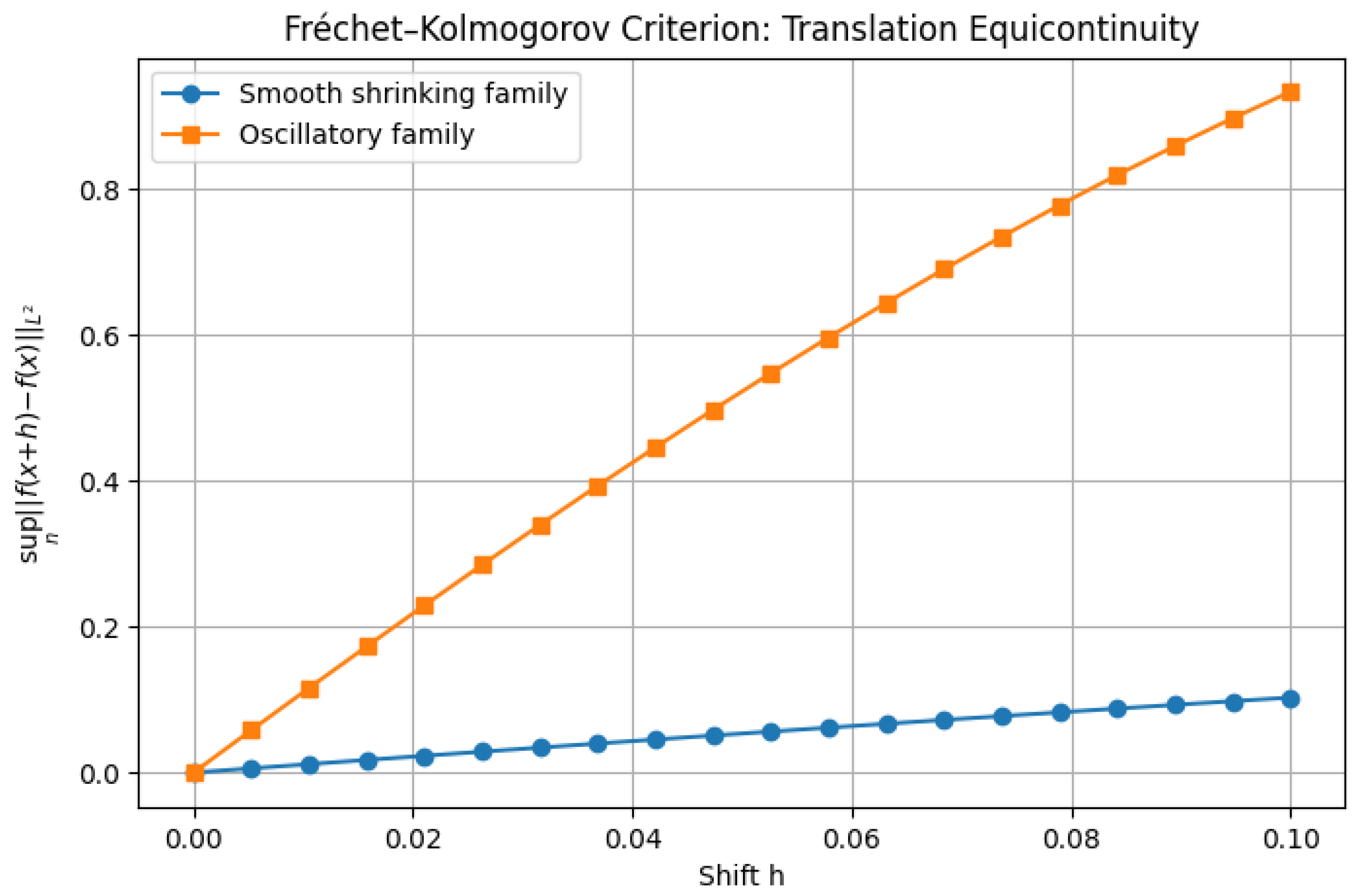
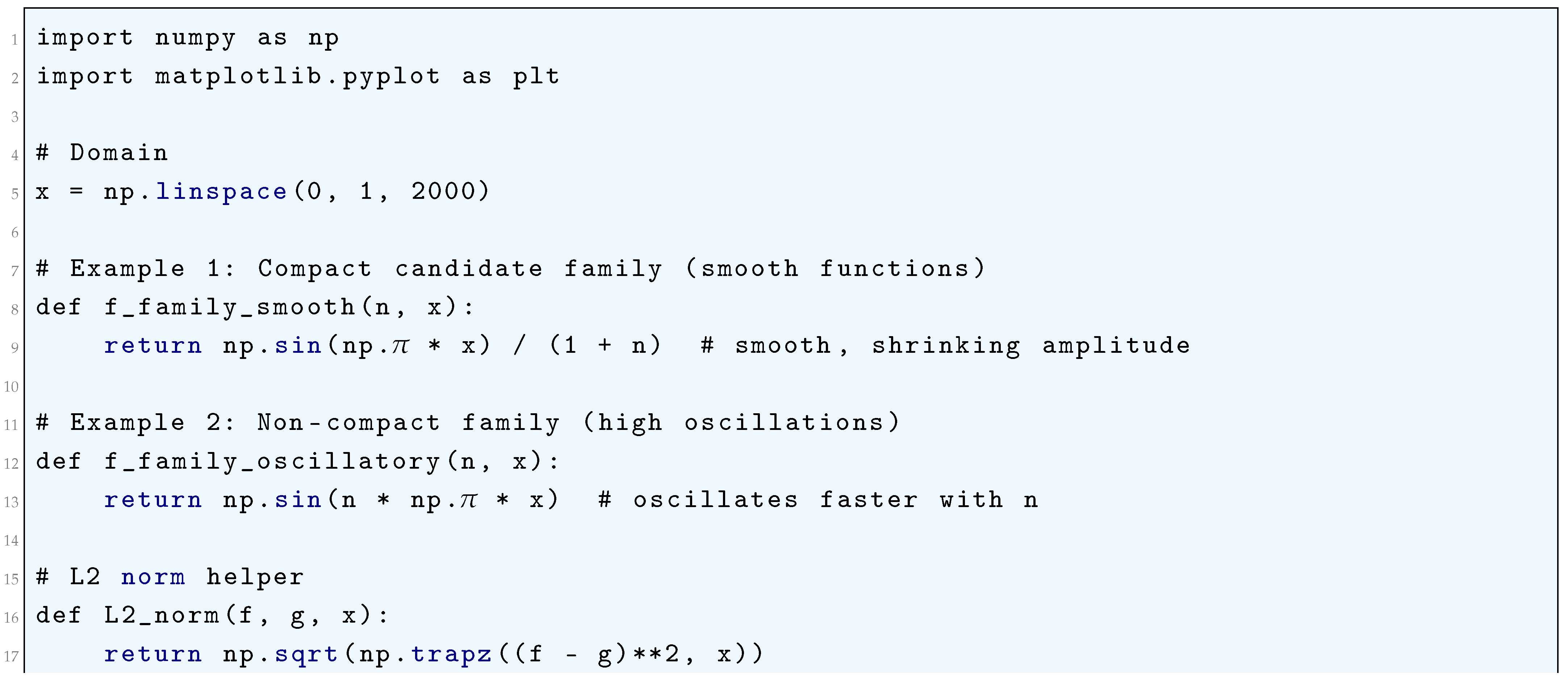
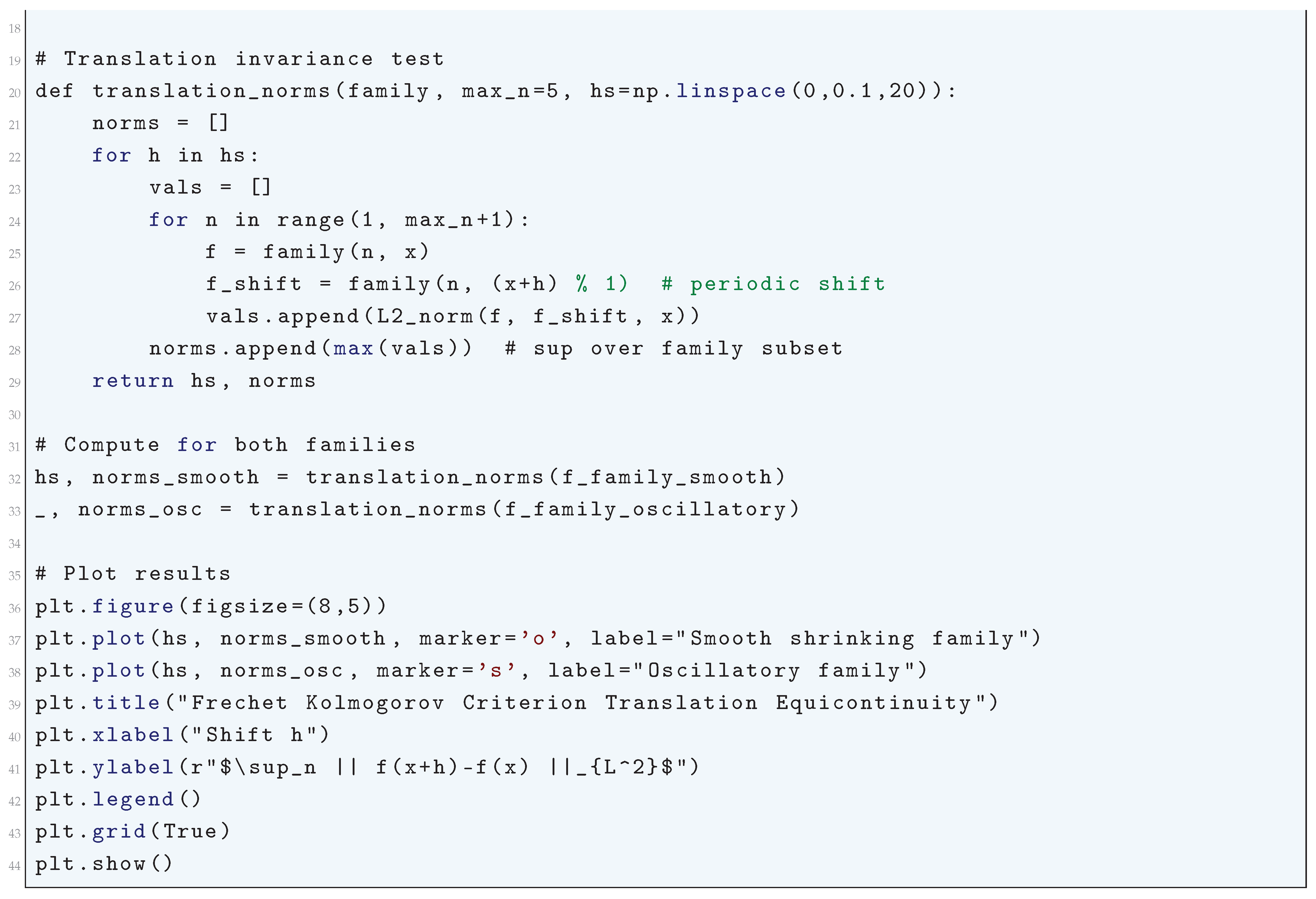
1.2.5.3 Python Code to Generate Figure 12
The Python code below produces the Figure 12 illustrating the Fréchet-Kolmogorov compactness criterion.
Figure 12.
Fréchet–Kolmogorov Criterion: Translation Equicontinuity
1.2.6. Sobolev-Poincaré Inequality
1.2.6.1 Literature Review of Sobolev-Poincaré Inequality
The Sobolev-Poincaré inequality is a cornerstone of modern analysis with far-reaching applications across partial differential equations, geometric analysis, and metric geometry. Among the most comprehensive treatments is Vladimir Maz’ya’s (1985) [1559] seminal work, which provides an exhaustive study of Sobolev-type inequalities including sharp constants, capacity theory, and their validity on both smooth and irregular domains. This foundational text is complemented by Haim Brezis’s (2011) [1549] contribution, which situates the inequality within functional analysis and PDE theory, particularly emphasizing its role in compact embeddings and elliptic regularity. The geometric aspects are profoundly explored in Mikhail Gromov’s (1999) [1555] work, extending classical results to general metric measure spaces, while Elliott Lieb and Michael Loss’s (2001) [1558] analysis offers crucial insights into optimal constants and connections with isoperimetric inequalities through real analytic methods. Heinonen’s (2001)[1563] lectures on analysis on metric spaces also discuss the Sobolev-Poincaré inequality and its application in various mathematical topics in great depth.
For applications to partial differential equations, David Gilbarg and Neil Trudinger’s (2001) [1562] treatment remains indispensable for its rigorous examination of local and global versions on bounded domains, particularly in regularity theory. The variational perspective appears prominently in Antonio Ambrosetti and Andrea Malchiodi’s (2007) [1546] study, which demonstrates how the inequality underpins existence results for nonlinear PDEs. In geometric contexts, Pierre Buser’s (1982) [1550] research on Riemannian manifolds establishes precise relationships between Poincaré constants and geometric data like curvature and diameter, whereas Nicola Garofalo and Dariusz Z. D’Agostino’s (1999) [1554] contributions derive sharp inequalities for sub-Riemannian structures. The probabilistic and geometric-analytic connections are masterfully presented in Dominique Bakry, Ivan Gentil, and Michel Ledoux’s (2014) [1547] work, linking the inequality to Markov semigroups and curvature-dimension conditions.
The extension to nonsmooth settings is systematically developed in Juha Heinonen and Pekka Koskela’s (2001, 2005) [1556][1557] research, which reformulates the inequality using upper gradients for applications in fractal and sub-Riemannian geometry. Luigi Ambrosio, Nicola Gigli, and Giuseppe Savaré’s (2005, 2008) [1544][1545] contributions provide groundbreaking syntheses with optimal transport and metric measure space theory. Hypoelliptic settings are addressed in Luca Capogna, Donatella Danielli, and Nicola Garofalo’s (2001) [1551] work on Hörmander vector fields, while Fabrice Baudoin and Michel Bonnefont’s (2012) [1548] research extends these to subelliptic operators. The heat kernel and spectral perspectives are thoroughly examined in E. Brian Davies’s (1989) [1552] investigation and Qi S. Zhang’s (2011) [1561] work on Ricci flow. Further abstract formulations appear in Karl-Theodor Sturm and Max-K. von Renesse’s (2005) [1560] optimal transport approach to curvature bounds, and Herbert Federer’s (1969) [1553] study provides essential links to currents and varifolds. Collectively, these works form a multifaceted theoretical edifice, demonstrating the Sobolev-Poincaré inequality’s central role in analysis, geometry, and probability through diverse yet interconnected perspectives.
1.2.6.2 Analysis of Sobolev-Poincaré Inequality
Let be a bounded domain with a Lipschitz boundary. Consider the Sobolev space for , which consists of functions whose weak derivatives also belong to . The Sobolev-Poincaré inequality asserts the existence of a constant such that
for all , where is the Sobolev conjugate exponent and is the mean value of u over , given by
To prove this inequality, we first use a representation formula for . Given any two points , we consider the fundamental theorem of calculus applied along the segment connecting x to y. Define the parametrization
Applying the fundamental theorem of calculus along this line segment,
By the chain rule,
Substituting this into the integral expression,
Taking the absolute value and applying Hölder’s inequality with conjugate exponents p and ,
Now, integrating both sides over , using Fubini’s theorem and Minkowski’s integral inequality,
Using the properties of integral norms and applying Hölder’s inequality again,
By averaging over and defining the mean-value term appropriately, we obtain
where C depends on and p, completing the proof.
Let be a bounded domain with a Lipschitz boundary. Consider the Sobolev space for , which consists of functions whose weak derivatives also belong to . The Sobolev-Poincaré inequality asserts the existence of a constant such that
for all , where is the Sobolev conjugate exponent and is the mean value of u over , given by
To prove this inequality, we first use a representation formula for . Given any two points , we consider the fundamental theorem of calculus applied along the segment connecting x to y. Define the parametrization
Applying the fundamental theorem of calculus along this line segment,
By the chain rule,
Substituting this into the integral expression,
Taking the absolute value and applying Hölder’s inequality with conjugate exponents p and ,
Now, integrating both sides over , using Fubini’s theorem and Minkowski’s integral inequality,
Using the properties of integral norms and applying Hölder’s inequality again,
By averaging over and defining the mean-value term appropriately, we obtain
where C depends on and p, completing the proof. The consequences and applications are:
- Regularity of PDE Solutions: The Sobolev-Poincaré inequality is crucial in proving the existence and regularity of weak solutions to elliptic PDEs.
- Compactness and Rellich-Kondrachov Theorem: It plays a role in proving the compact embedding of into , which is fundamental in functional analysis.
- Control of Function Oscillations: It quantifies how much a function can deviate from its mean, which is used in various areas of mathematical physics and geometry.
One important extension is the sharp form of the Sobolev-Poincaré inequality, which involves explicit best constants in terms of the domain geometry. Specifically, in some cases, the optimal constant is related to eigenvalues of the Laplace operator or geometric properties such as the diameter or inradius of . Another important extension is the fractional Sobolev-Poincaré inequality, which deals with function spaces like where s is fractional, incorporating nonlocal effects.
In conclusion, the Sobolev-Poincaré inequality is a powerful mathematical result that provides a precise relationship between function averages and their gradients. It is a cornerstone in modern analysis, with deep implications in PDE theory, functional analysis, and geometric measure theory.
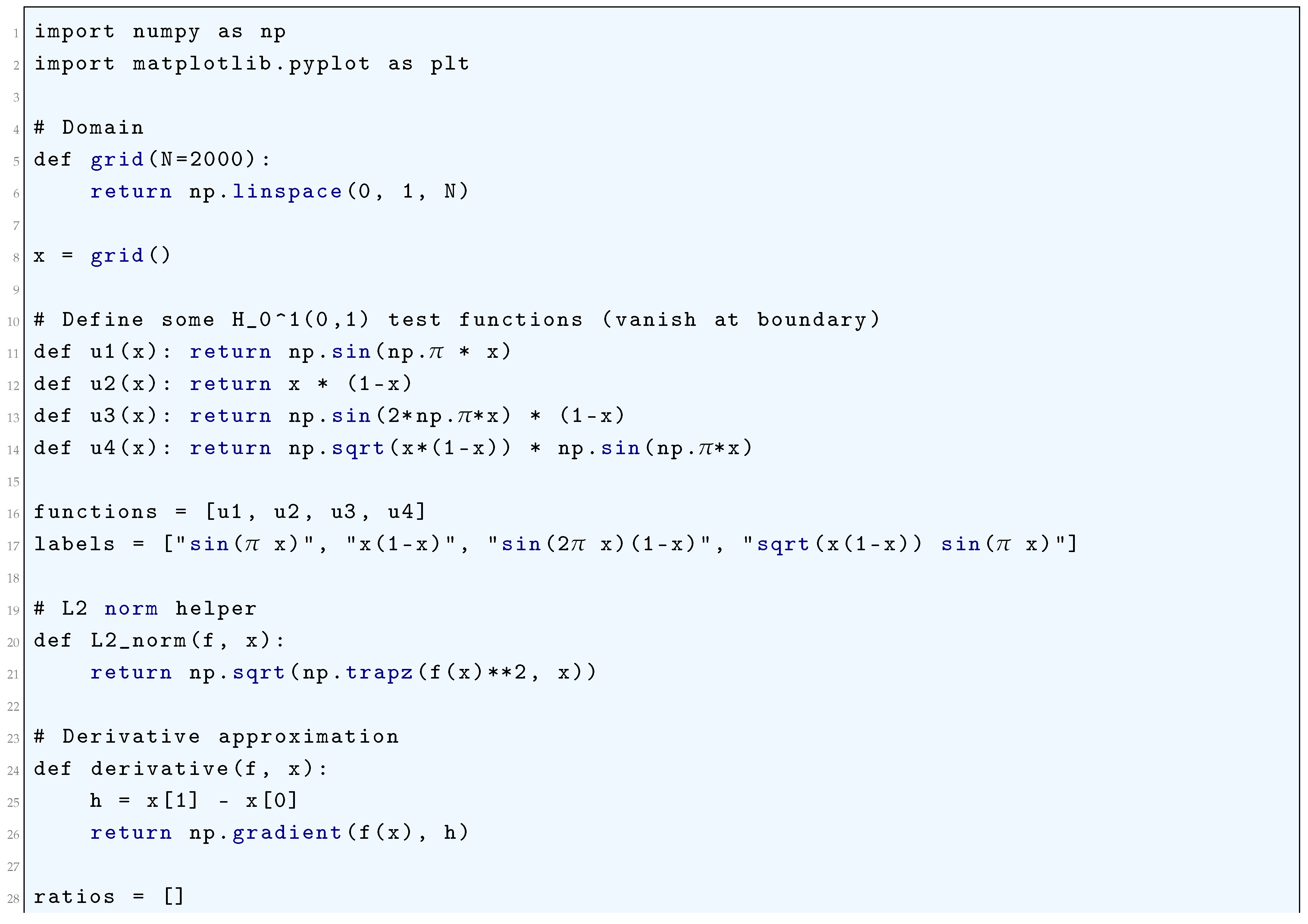
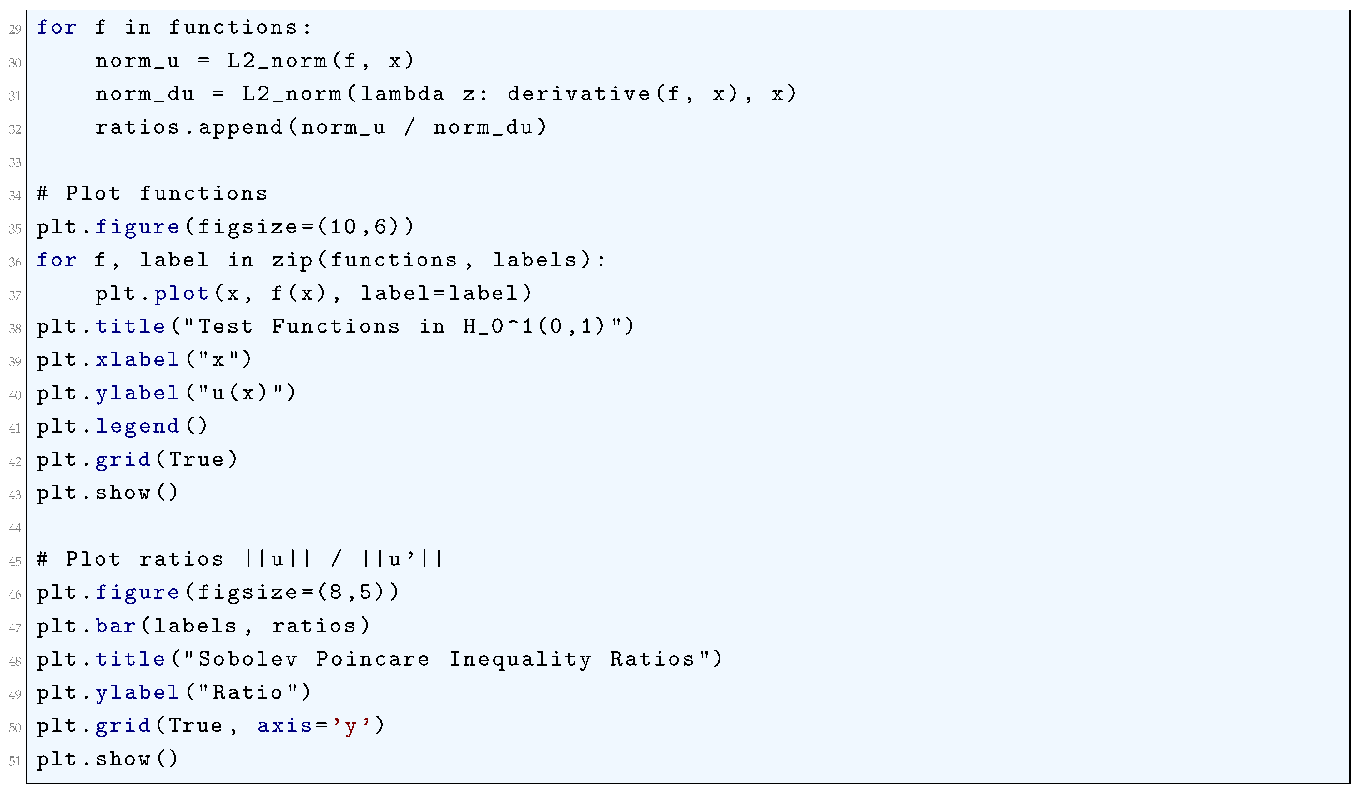
1.2.6.3 Python Code to Generate Figure 13 and Figure 14
The Python code below produces the Figure 13 and Figure 14 illustrating the Fréchet-Kolmogorov compactness criterion.
Figure 13.
Test Functions in
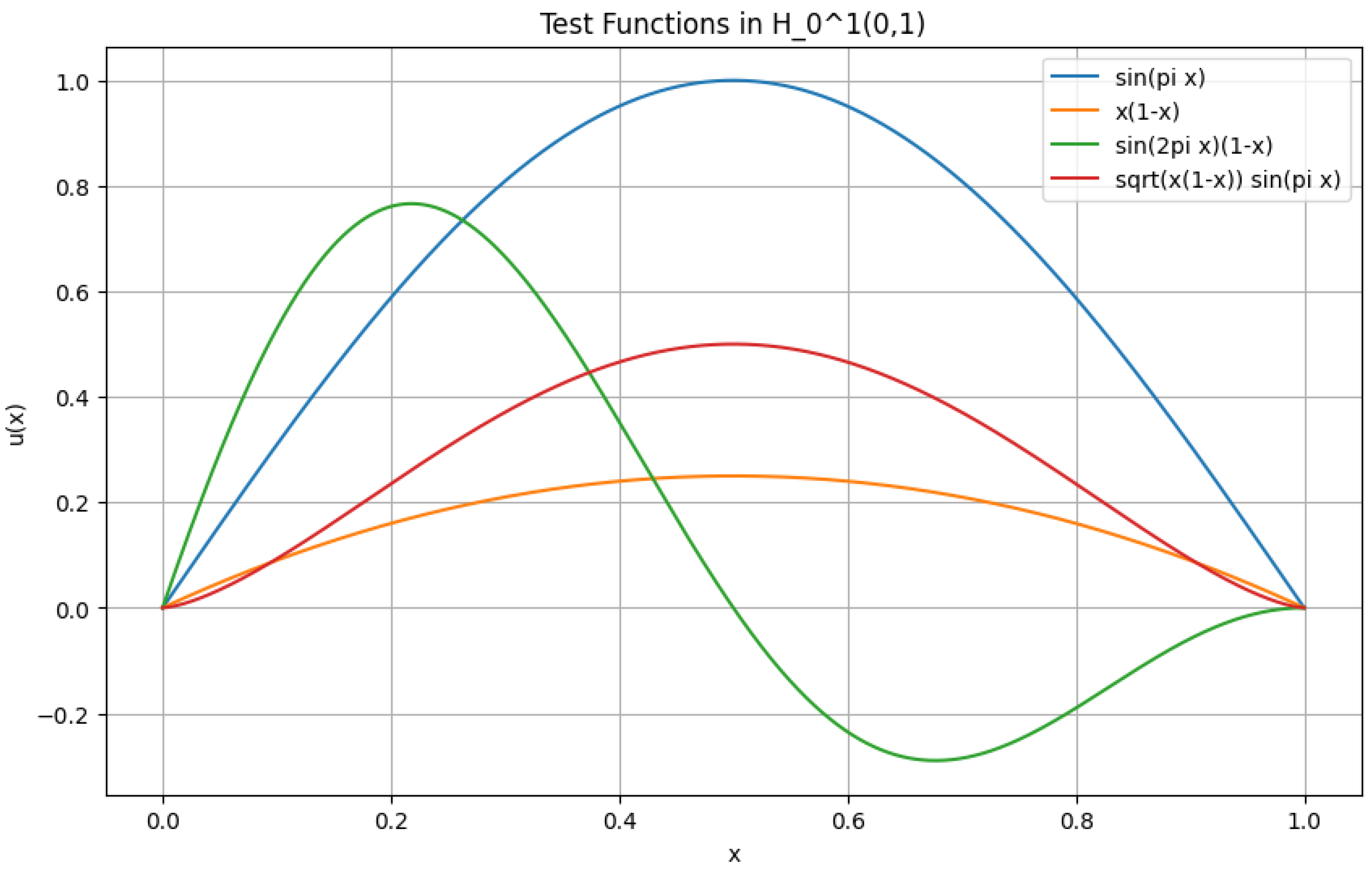
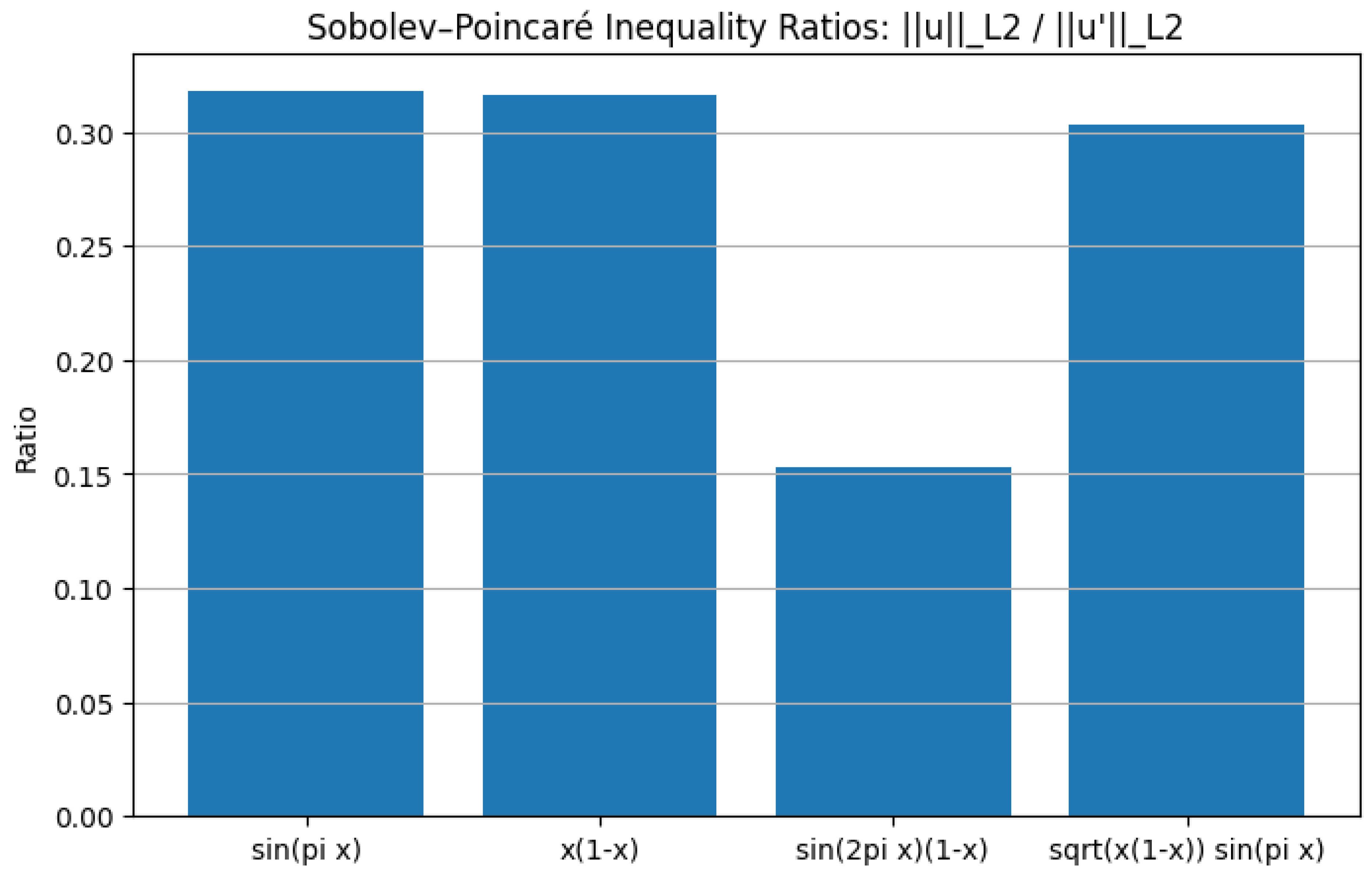
Figure 14.
Sobolev–Poincaré Inequality Ratios:
2. Universal Approximation Theorem: Refined Proof
The Universal Approximation Theorem (UAT) is a fundamental result in neural network theory, stating that a feedforward neural network with a single hidden layer containing a finite number of neurons can approximate any continuous function on a compact subset of to any desired degree of accuracy, provided that an appropriate activation function is used. This theorem has significant implications in machine learning, function approximation, and deep learning architectures.
The Universal Approximation Theorem (UAT) is a fundamental result in the theory of artificial neural networks, which states that a feedforward neural network with a single hidden layer and a non-polynomial activation function can approximate any continuous function on a compact subset of to arbitrary precision, provided the hidden layer has a sufficient number of neurons. Formally, let be a non-constant, bounded, and continuous activation function. For any continuous function defined on a compact set K, and for every , there exists a neural network of the form:
where N is the number of hidden units, are the input weights, are the biases, and are the output weights, such that:
The theorem underscores the expressive power of neural networks, demonstrating that even a single hidden layer is theoretically capable of approximating any continuous function, given enough neurons. The key assumptions are the non-polynomial nature of the activation function and the compactness of the domain. Common activation functions satisfying these conditions include the sigmoid , the hyperbolic tangent , and the rectified linear unit (ReLU) . The compactness requirement ensures that the function f is uniformly continuous, enabling the approximation to hold uniformly across the entire domain. The proof of the UAT typically relies on tools from functional analysis, such as the Stone-Weierstrass theorem or the Hahn-Banach theorem, which guarantee the density of certain function spaces. For instance, the Stone-Weierstrass theorem asserts that any subalgebra of continuous functions that separates points and contains the constant functions is dense in the space of continuous functions. By showing that the set of functions representable by a neural network forms such a subalgebra, the UAT can be derived. The non-polynomial condition on is critical to ensure the network can generate a rich enough class of functions to approximate arbitrary continuous mappings.
However, the theorem does not provide explicit bounds on the number of neurons N required to achieve a given accuracy , nor does it address the practical challenges of training such networks. In practice, deeper architectures with multiple hidden layers often outperform shallow networks, even though the UAT theoretically guarantees the sufficiency of a single hidden layer. This discrepancy highlights the difference between existence and learnability: while the UAT ensures the existence of an approximating network, finding such a network through optimization remains a non-trivial task. The theorem also does not account for the curse of dimensionality, which can make the required number of neurons infeasibly large for high-dimensional inputs. Despite these limitations, the UAT remains a cornerstone of neural network theory, providing a rigorous foundation for their universal applicability.
2.1. Literature Review of Universal Approximation Theorem
Hornik et. al. (1989) [58] in their seminal paper rigorously proved that multilayer feedforward neural networks with a single hidden layer and a sigmoid activation function can approximate any continuous function on a compact set. It extends prior results and lays the foundation for the modern understanding of UAT. Cybenko (1989) [60] provided one of the first rigorous proofs of the UAT using the sigmoid function as the activation function. They demonstrated that a single hidden layer network can approximate any continuous function arbitrarily well. Barron (1993) [61] extended UAT by quantifying the approximation error and analyzing the rate of convergence. This work is crucial for understanding the practical efficiency of neural networks. Pinkus (1999) [62] provided a comprehensive survey of UAT from the perspective of approximation theory and also discussed conditions for approximation with different activation functions and the theoretical limits of neural networks. Lu et.al. (2017) [63] investigated how the width of neural networks affects their approximation capability, challenging the notion that deeper networks are always better. They also provided insights into trade-offs between depth and width. Hanin and Sellke (2018) [64] extended UAT to ReLU activation functions, showing that deep ReLU networks achieve universal approximation while maintaining minimal width constraints. Garcıa-Cervera et. al. (2024) [66] extended the universal approximation theorem to set-valued functions and its applications to Deep Operator Networks (DeepONets), which are useful in control theory and PDE modeling. Majee et.al. (2024) [67] explored the universal approximation properties of deep neural networks for solving inverse problems using Markov Chain Monte Carlo (MCMC) techniques. Toscano et. al. (2024) [68] introduced Kurkova-Kolmogorov-Arnold Networks (KKANs), an extension of UAT incorporating Kolmogorov’s superposition theorem for improved approximation capabilities. Son (2025) [69] established a new framework for operator learning based on the UAT, providing a theoretical foundation for backpropagation-free deep networks.
2.2. Approximation Using Convolution Operators
Let us begin by considering the convolution operator and its role in approximating functions in the context of the Universal Approximation Theorem (UAT). Suppose is a continuous and bounded function. The convolution of f with a kernel function , denoted as , is defined as
The kernel is typically chosen to be smooth, compactly supported, and normalized such that
To approximate f locally, we introduce a scaling parameter and define the scaled kernel as
The factor ensures that remains a probability density function, satisfying
The convolution of f with the scaled kernel is given by
Performing the change of variables , we have and . Substituting into the integral, we obtain
This representation shows that is a smoothed version of , where the smoothing is controlled by the parameter . As , the kernel becomes increasingly concentrated around x, and we recover in the limit:
assuming f is continuous.
This result can be rigorously proven using properties of the kernel , such as its smoothness and compact support, and the dominated convergence theorem, which ensures that the integral converges uniformly to . Now, let us consider the role of convolution operators in the approximation of f by neural networks. A single-layer feedforward neural network is expressed as
where are coefficients, are weight vectors, are biases, and is the activation function. The activation function can be interpreted as a localized response function, analogous to the kernel in convolution. By drawing an analogy between the two, we can write the neural network approximation as
where is interpreted as a parameterized kernel defined by , , and , and represents a discretization step. The approximation error can be decomposed into two components:
The term represents the error introduced by smoothing f with the kernel , and it can be made arbitrarily small by choosing sufficiently small, provided f is regular enough (e.g., Lipschitz continuous).
The term quantifies the error due to discretization, which vanishes as the number of neurons . To rigorously analyze the convergence of to , we rely on the density of neural network approximators in function spaces. The Universal Approximation Theorem states that, for any continuous function f on a compact domain and any , there exists a neural network with finitely many neurons such that
This result hinges on the ability of the activation function to generate a rich set of basis functions. For example, if (ReLU), the network approximates by piecewise linear functions. If (sigmoid), the network generates smooth approximations that resemble logistic regression.
In this refined proof of the UAT, convolution operators provide a unifying framework for understanding the smoothing, localization, and discretization processes that underlie neural network approximations. The interplay between , , and reveals the profound mathematical structure that connects classical approximation theory with modern machine learning. This connection not only enhances our theoretical understanding of neural networks but also guides the design of architectures and algorithms for practical applications.
2.2.1. Python Code to Generate Figure 15 and Figure 16
The Python code below produces the Figure 15 and Figure 16 illustrating the Approximation Using Convolution Operators.
Figure 15.
Universal Approximation Theorem Illustration
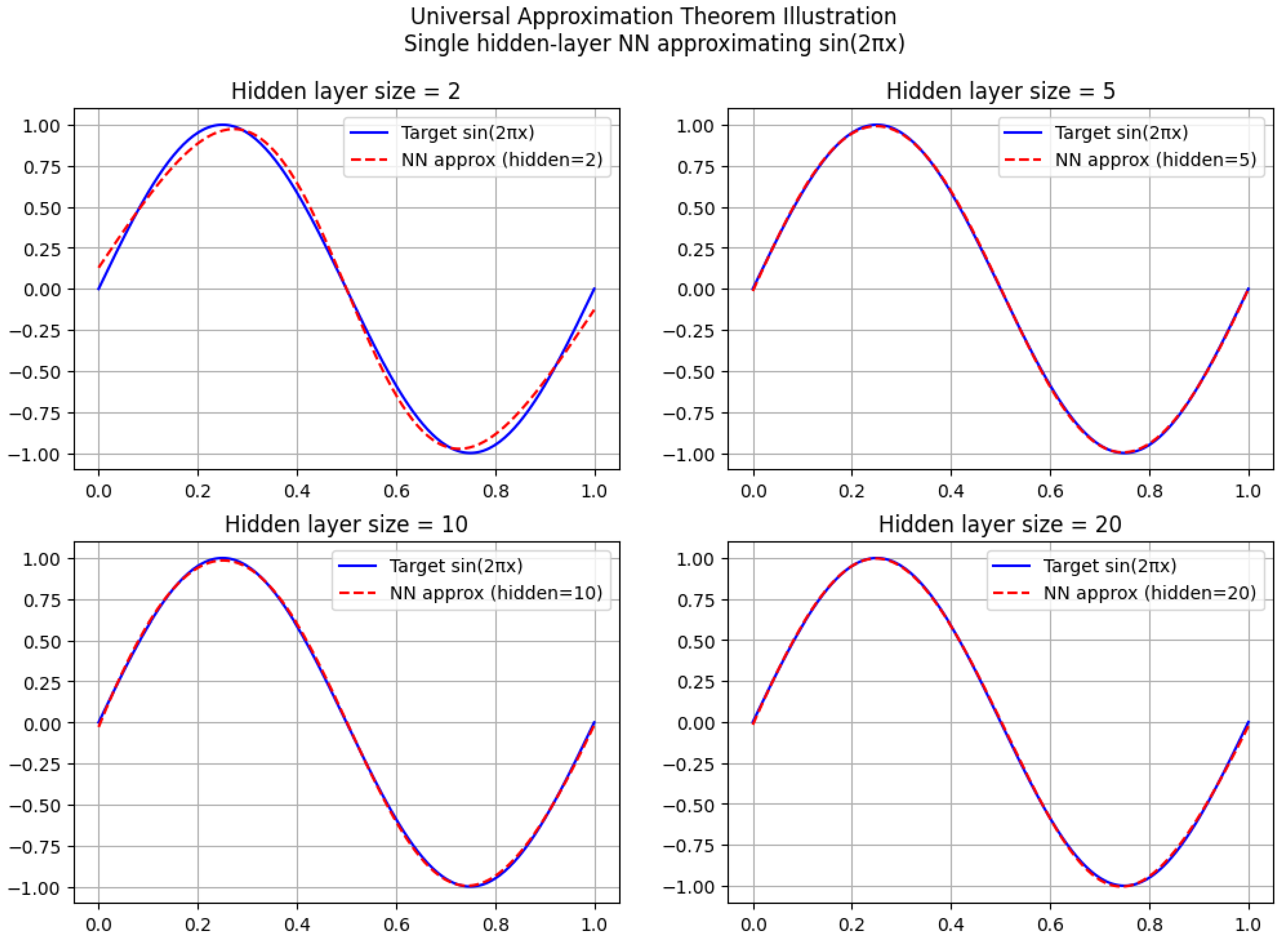
Figure 16.
Approximation Error vs Hidden Layer Size
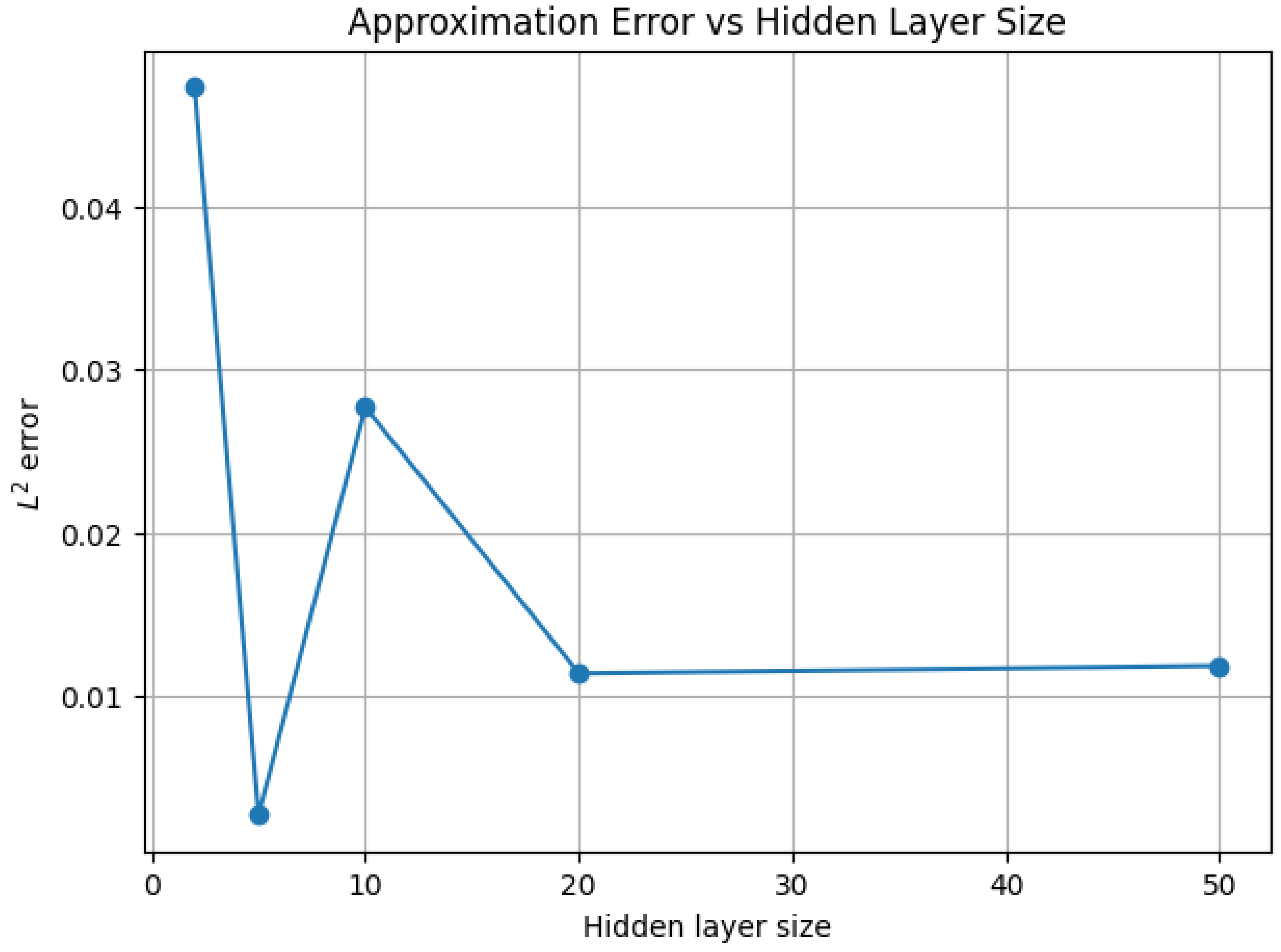
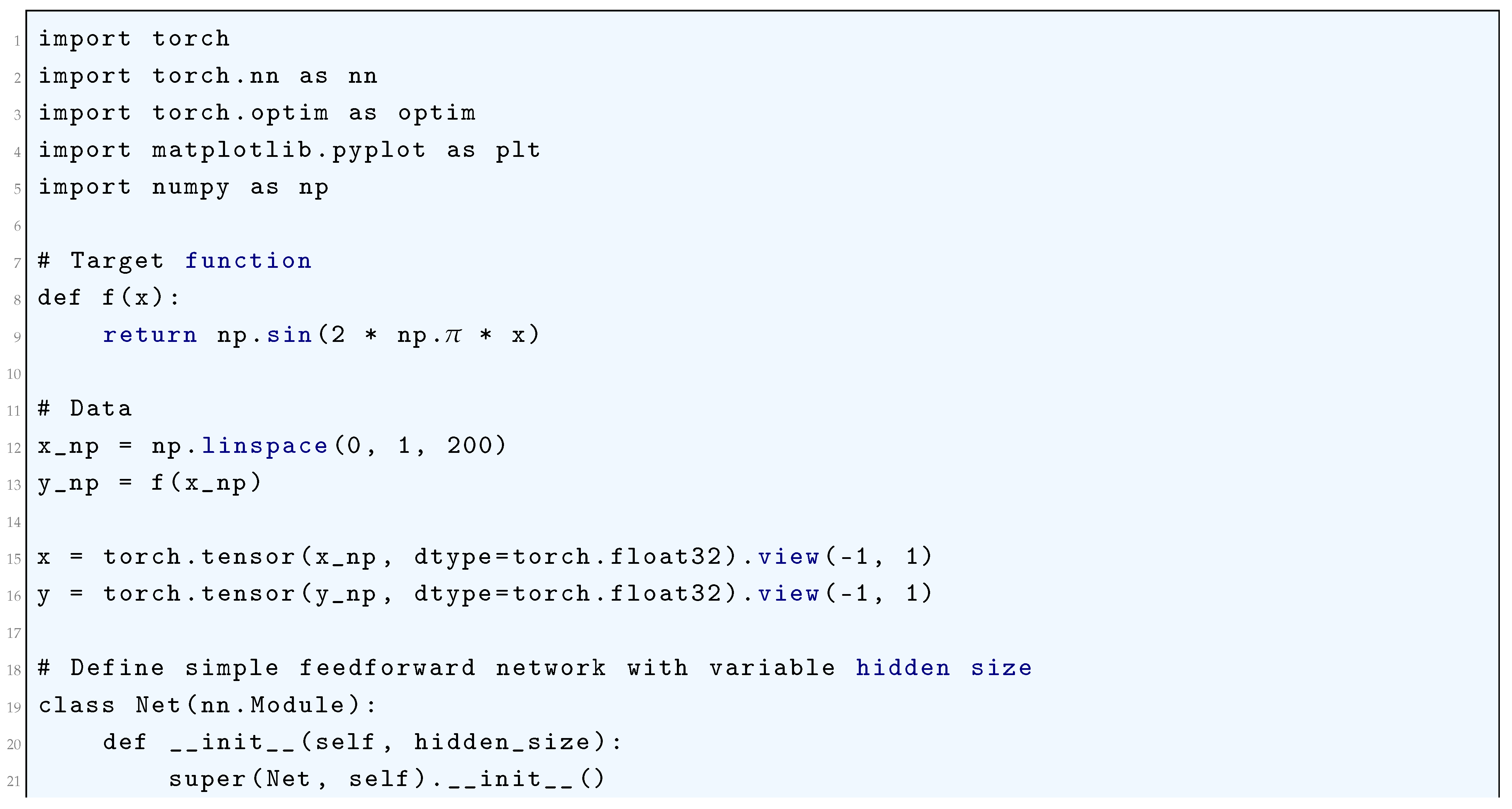
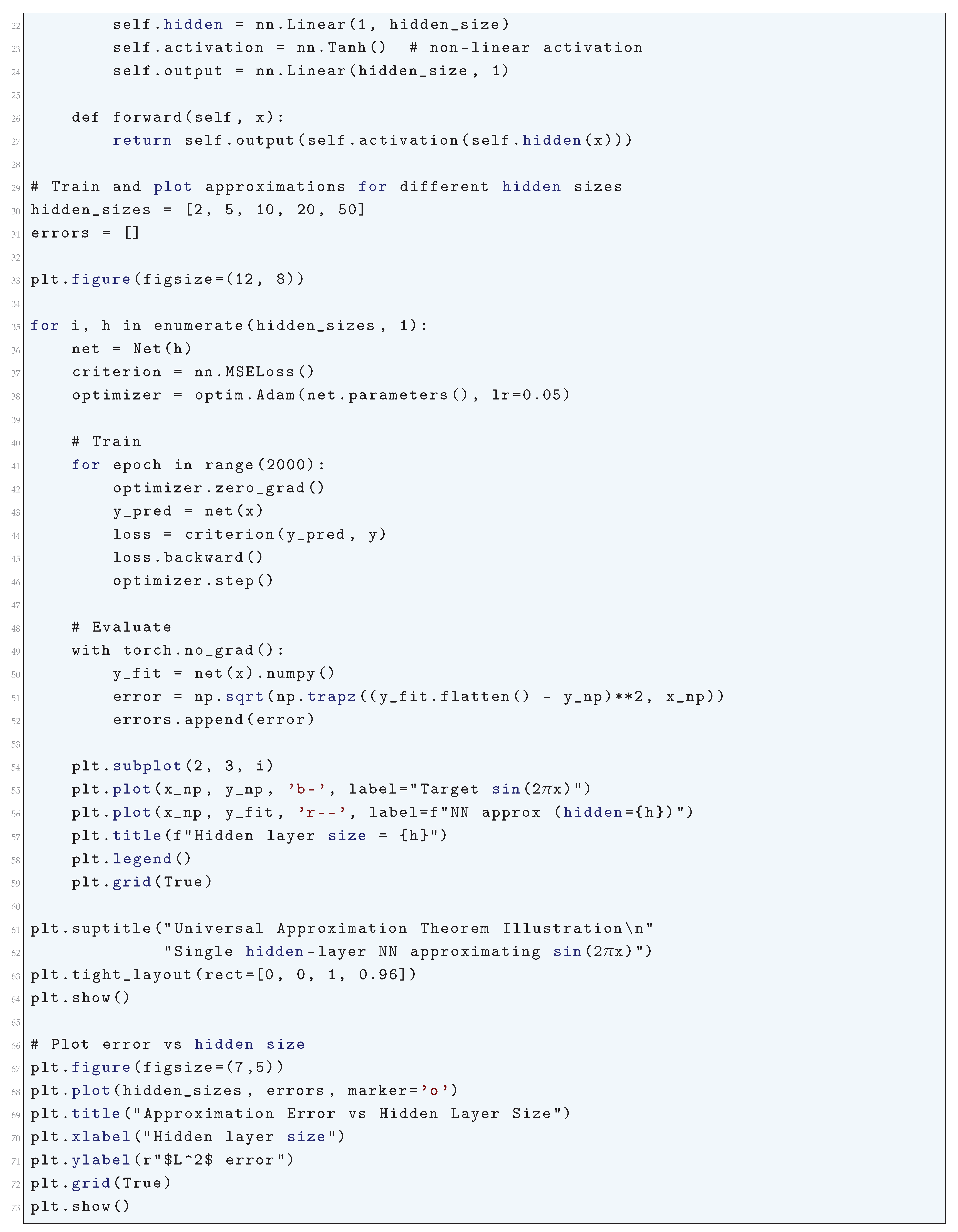
2.2.2. Stone-Weierstrass Application
2.2.2.1 Literature Review of Stone-Weierstrass Application
Rudin (1976) [70] introduced the Weierstrass approximation theorem and proves its generalization, the Stone-Weierstrass theorem. He also discussed the algebraic structure of function spaces and how the theorem ensures the uniform approximation of continuous functions by polynomials. He also presented examples and exercises related to compactness, uniform convergence, and Banach algebra structures. Stein and Shakarchi (2005) [71] extended the Stone-Weierstrass theorem into measure theory and functional analysis. He also proved the theorem in the context of Lebesgue integration. He also discussed how it applies to Hilbert spaces and orthogonal polynomials. He also connected the theorem to Fourier analysis and spectral decomposition. Conway (2019) [73] explored the Stone-Weierstrass theorem in the setting of Banach algebras and C-algebras*. He also extended the theorem to non-commutative function algebras and discussed the operator-theoretic implications of the theorem in Hilbert spaces. He also analyzed the theorem’s application to spectral theory. Dieudonné (1981) [74] traced the historical development of functional analysis, including the origins of the Stone-Weierstrass theorem and discussed contributions by Karl Weierstrass and Marshall Stone. He also explored how the theorem influenced topological vector spaces and operator theory and also included perspectives on the axiomatic development of function approximation. Folland (1999) [76] discussed the Stone-Weierstrass theorem in depth with applications to probability theory and ergodic theory and used the theorem to establish the density of algebraic functions in measure spaces He also connected the Stone-Weierstrass theorem to functional approximation in Lp spaces. He also explored the interplay between the Stone-Weierstrass theorem and the Hahn-Banach theorem. Sugiura (2024) [77] extended the Stone-Weierstrass theorem to the study of reservoir computing in machine learning and proved that certain neural networks can approximate functions uniformly under the assumptions of the theorem. He bridges classical functional approximation with modern AI and deep learning. Liu et al. (2024) [78] investigated the Stone-Weierstrass theorem in normed module settings and used category theory to generalize function approximation results. He also extended the theorem beyond real-valued functions to structured mathematical objects. Martinez-Barreto (2025) [79] provided a modern formulation of the theorem with rigorous proof and reviewed applications in operator algebras and topology. He also discussed open problems related to function approximation. Chang and Wei (2024) [80] used the Stone-Weierstrass theorem to derive new operator inequalities and applied the theorem to functional analysis in quantum mechanics. Caballer et al. (2024) [81] investigated cases where the Stone-Weierstrass theorem fails and provided counterexamples and refined conditions for uniform approximation. Chen (2024) [82] extended the Stone-Weierstrass theorem to generalized function spaces and introduced a new class of uniform topological algebras. Rafiei and Akbarzadeh-T (2024) [83] used the Stone-Weierstrass theorem to analyze function approximation in fuzzy logic systems and explored the applications in control systems and AI.
2.2.2.2 Analysis of Stone-Weierstrass Application
The Stone-Weierstrass Theorem serves as a cornerstone in functional analysis, bridging the algebraic structure of continuous functions with approximation theory. This theorem, when applied to the Universal Approximation Theorem (UAT), provides a rigorous foundation for asserting that neural networks can approximate any continuous function defined on a compact set. To understand this connection in its most scientifically and mathematically rigorous form, we must carefully analyze the algebra of continuous functions on a compact Hausdorff space and the role of neural networks in approximating these functions, ensuring that all mathematical nuances are explored with extreme precision. Let X be a compact Hausdorff space, and let represent the space of continuous real-valued functions on X. The supremum norm for a function is defined as:
This supremum norm is critical in defining the proximity between continuous functions, as we seek to approximate any function by a function g from a subalgebra .
The Stone-Weierstrass theorem guarantees that if the subalgebra A satisfies two essential properties—(1) it contains the constant functions, and (2) it separates points—then the closure of A in the supremum norm will be the entire space . To formalize this, we define the point separation property as follows: for every pair of distinct points , there exists a function such that . This condition ensures that functions from A are sufficiently “rich” to distinguish between different points in X. Mathematically, this is expressed as:
Given these two properties, the Stone-Weierstrass theorem asserts that for any continuous function and any , there exists an element such that:
This result ensures that any continuous function on a compact Hausdorff space can be approximated arbitrarily closely by functions from a sufficiently rich subalgebra. In the context of the Universal Approximation Theorem (UAT), we seek to apply the Stone-Weierstrass theorem to the approximation capabilities of neural networks. Let be a compact subset, and let be a continuous function defined on this set. A feedforward neural network with a non-linear activation function has the form:
where represents the inner product between the weight vector and the input x, and represents the bias term. The activation function is typically non-linear (such as the sigmoid or ReLU function), and the parameters are the weights and biases of the network. The function is a weighted sum of the non-linear activations applied to the affine transformations of x.
We now explore the connection between neural networks and the Stone-Weierstrass theorem. A critical observation is that the set of functions defined by a neural network with non-linear activation is a subalgebra of provided the activation function is sufficiently rich in its non-linearity.
This non-linearity ensures that the network can separate points in K, meaning that for any two distinct points , there exists a network function that takes distinct values at these points. This satisfies the point separation condition required by the Stone-Weierstrass theorem. To formalize this, consider two distinct points . Since is non-linear, the function with appropriately chosen weights and biases will satisfy:
Thus, the algebra of neural network functions satisfies the point separation property. By applying the Stone-Weierstrass theorem, we conclude that this algebra is dense in , meaning that for any continuous function and any , there exists a neural network function such that:
This rigorous result shows that neural networks with a non-linear activation function can approximate any continuous function on a compact set arbitrarily closely in the supremum norm, thereby proving the Universal Approximation Theorem. To further explore this, consider the error term:
For a given function f and a compact set K, this error term can be made arbitrarily small by increasing the number of neurons in the hidden layer of the neural network. This increases the capacity of the network, effectively enlarging the subalgebra of functions generated by the network, thereby improving the approximation. As the number of neurons increases, the network’s ability to approximate any function from becomes increasingly precise, which aligns with the conclusion of the Stone-Weierstrass theorem that the network functions form a dense subalgebra in . Thus, the Universal Approximation Theorem, derived through the Stone-Weierstrass theorem, rigorously proves that neural networks can approximate any continuous function on a compact set to any desired degree of accuracy. The combination of the non-linearity of the activation function and the architecture of the neural network guarantees that the network can generate a dense subalgebra of continuous functions, ultimately allowing it to approximate any function from . This result not only formalizes the approximation power of neural networks but also provides a deep theoretical foundation for understanding their capabilities as universal approximators.
2.2.2.3 Python Code to Generate Figure 17, Figure 18 and Figure 19
The Python code below produces the Figure 17, Figure 18 and Figure 19 illustrating the Stone-Weierstrass Application.
Figure 17.
Stone–Weierstrass (Weierstrass) demo: Bernstein polynomial approximations
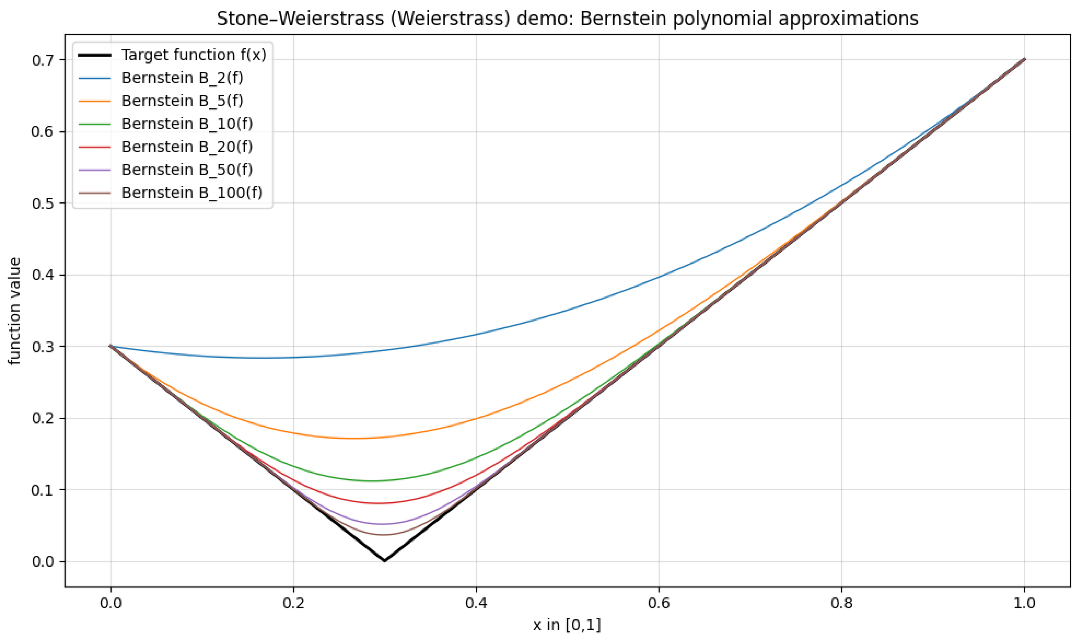
Figure 18.
Zoom near the kink — convergence is uniform
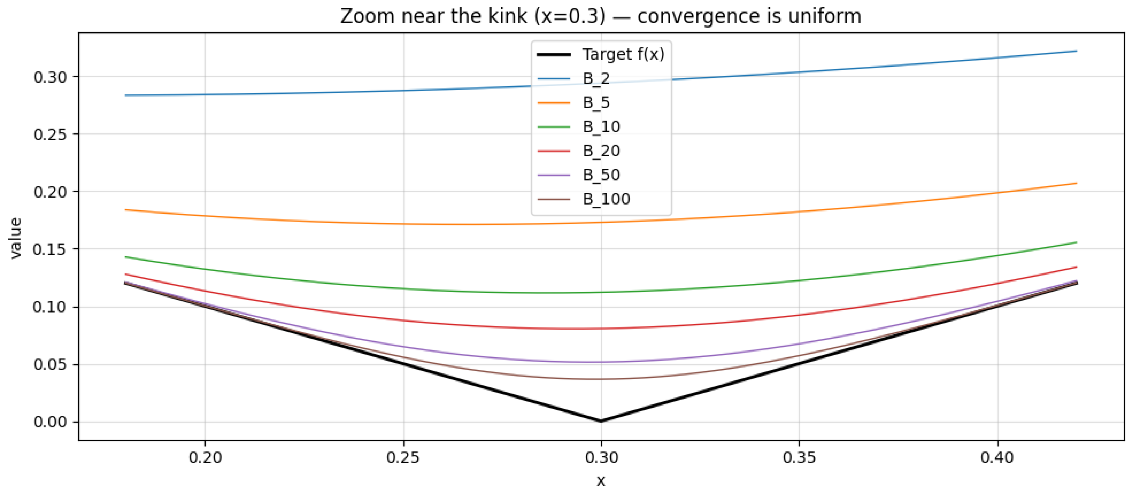
Figure 19.
Sup-norm error (log-log scale)
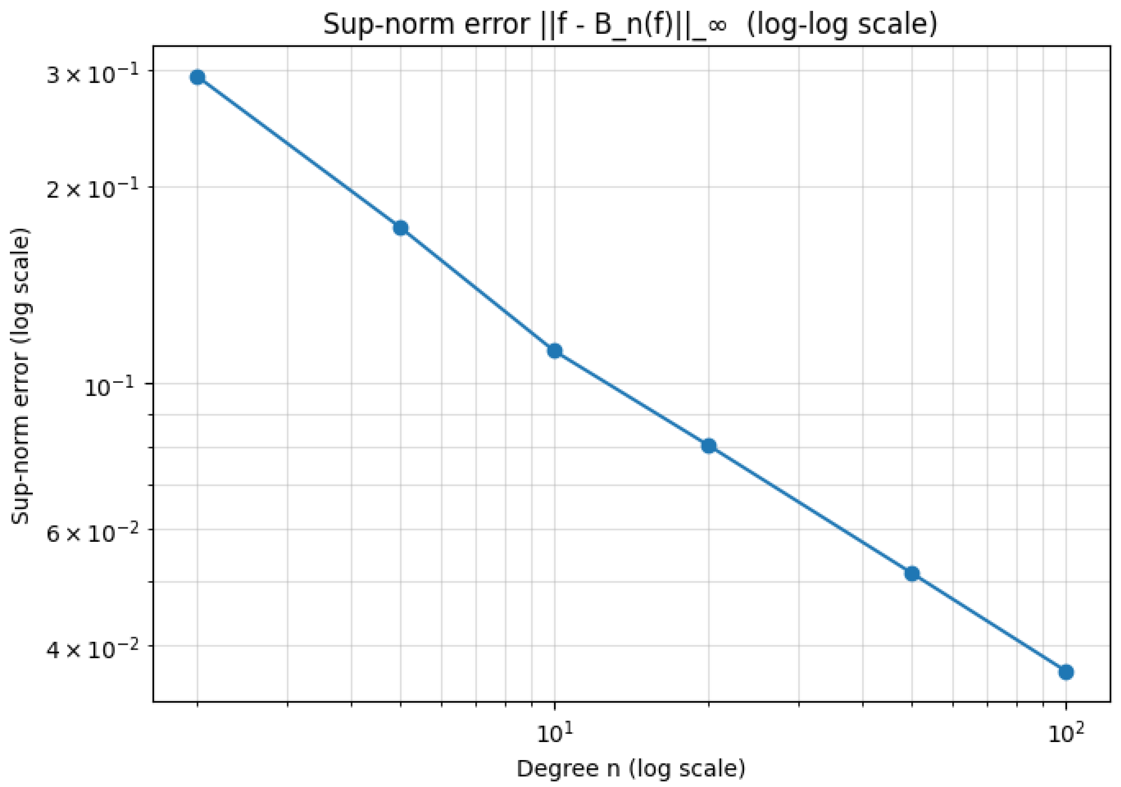
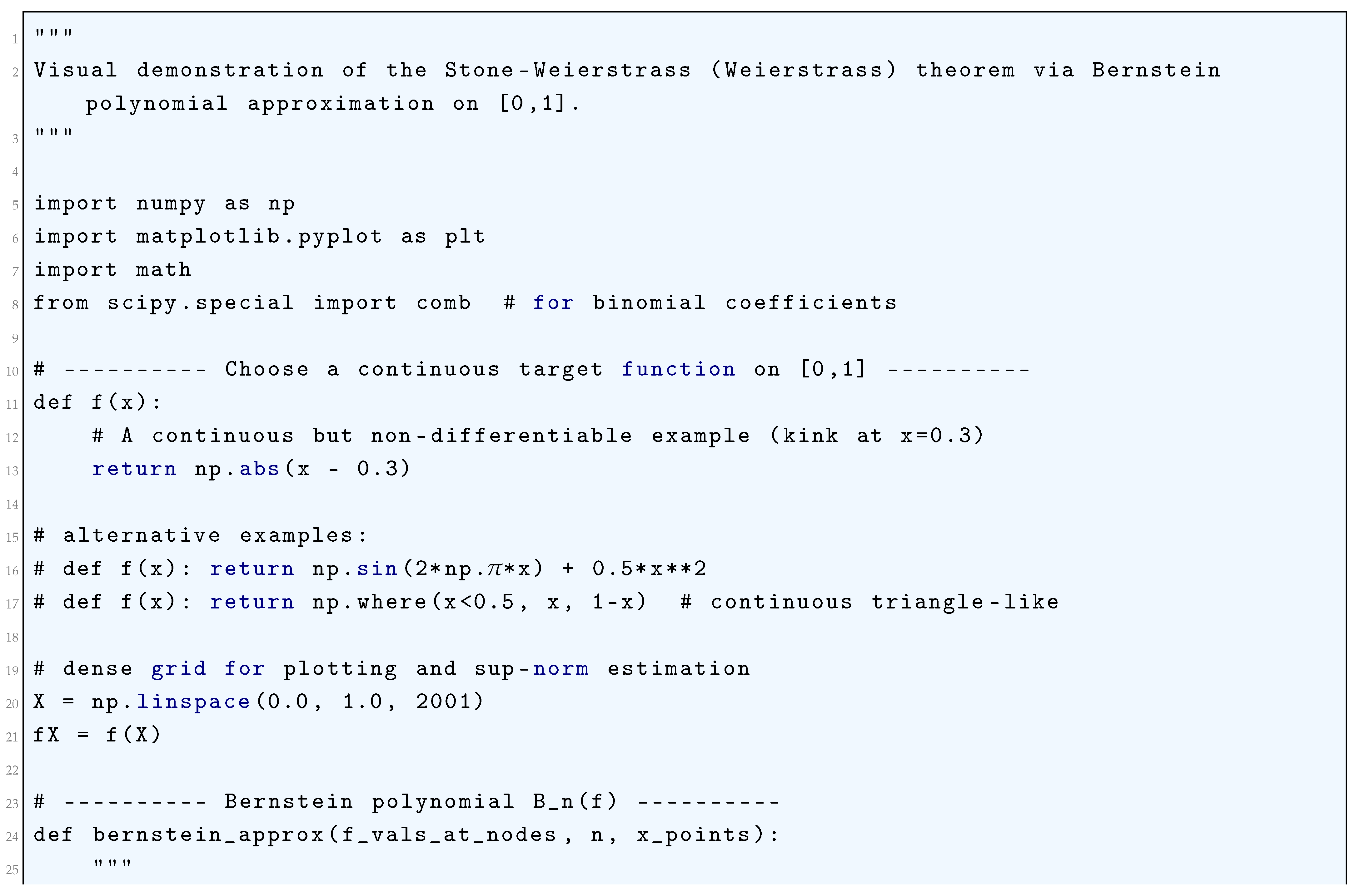
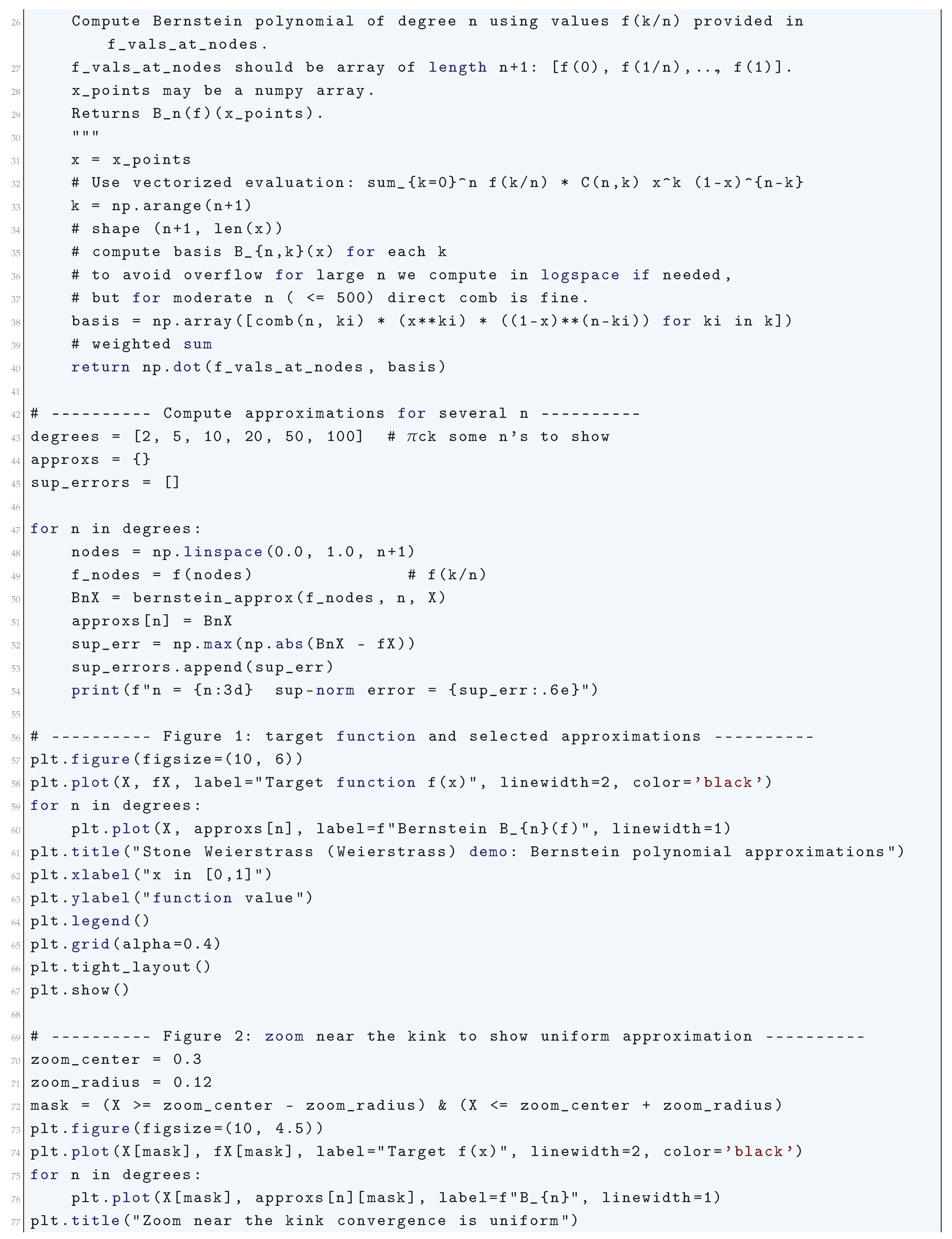
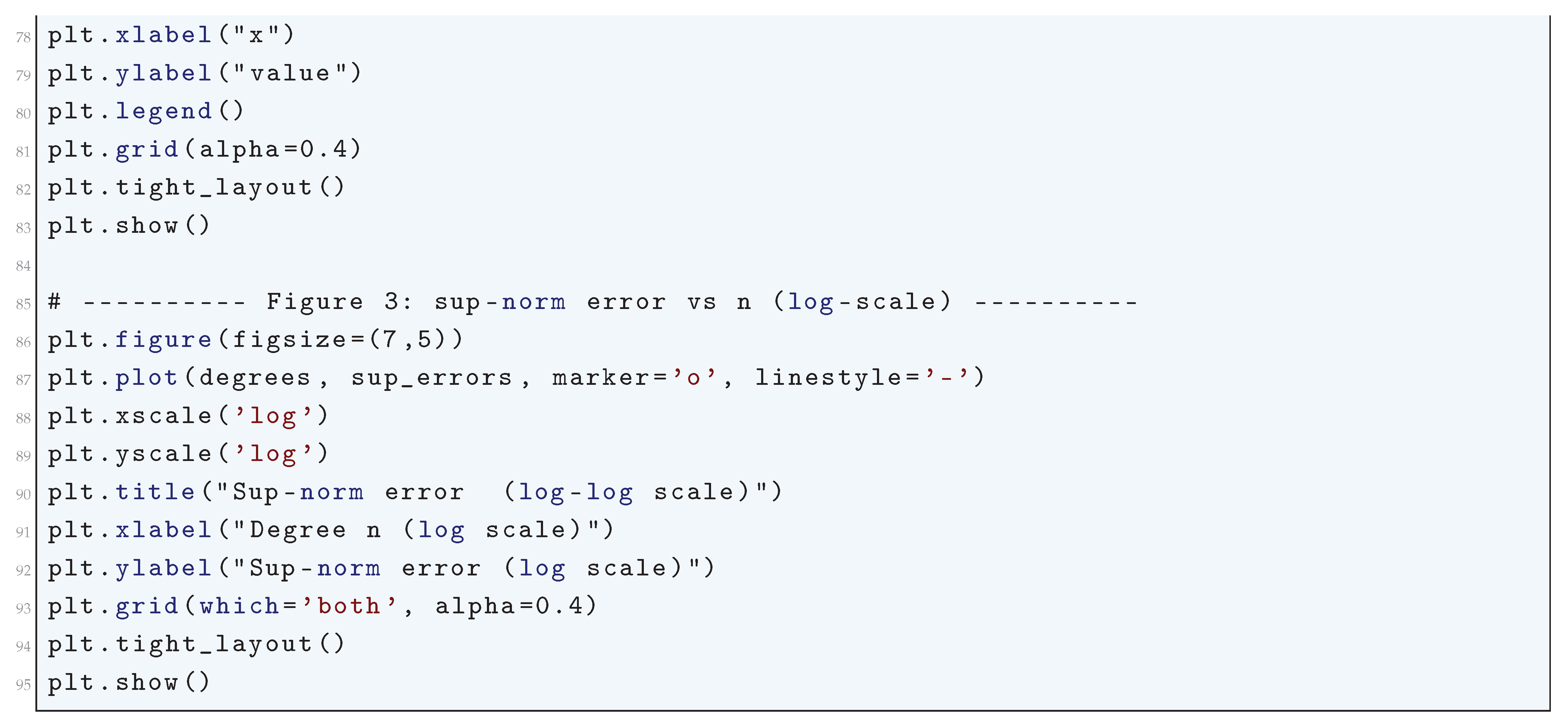
2.3. Depth vs. Width: Capacity Analysis
2.3.1. Bounding the Expressive Power
The Kolmogorov-Arnold Superposition Theorem is a foundational result in the mathematical analysis of multivariate continuous functions and their decompositions, providing a framework that underpins the expressive power of neural networks. It asserts that any continuous multivariate function can be expressed as a finite composition of continuous univariate functions and addition. It was first conjectured by Andrey Kolmogorov in 1956 and later rigorously proved by Vladimir Arnold in 1957. Formally, the theorem guarantees that any continuous multivariate function can be represented as a finite composition of continuous univariate functions and . Specifically, for , there exist functions and , such that
where the functions encode the univariate projections of the input variables , and the outer functions aggregate these projections into the final output. This decomposition highlights a fundamental property of multivariate continuous functions: their expressiveness can be captured through hierarchical compositions of simpler, univariate components.
2.3.1.1 Literature Review of Kolmogorov-Arnold Superposition Theorem
There are some Classical References on the Kolmogorov-Arnold Superposition Theorem (KST). Kolmogorov (1957) [84] in his Foundational Paper on KST established that any continuous function of several variables can be represented as a superposition of continuous functions of a single variable and addition. This was groundbreaking because it provided a universal function decomposition method, independent of inner-product spaces. He proved that there exist functions and such that any function can be expressed as:
where the are univariate functions. Kolmogorov provided a mathematical basis for approximation theory and neural networks, influencing modern machine learning architectures. Arnold (1963) [86] refined Kolmogorov’s theorem by proving that one can restrict the superposition to functions of at most two variables instead of one. Arnold’s formulation led to the Kolmogorov-Arnold representation:
making the theorem more suitable for practical computations. Arnold strengthened the expressivity of neural networks, inspiring alternative function representations in high-dimensional settings. Lorentz (2008) [87] in his book discusses the significance of KST in approximation theory and constructive mathematics. He provided error estimates for approximating multivariate functions using Kolmogorov-type decompositions. He showed how KST fits within Bernstein approximation theory. He helped frame KST in the context of function approximation, bridging it to computational applications. Building on this theoretical foundation, Hornik et. al. (1989) [58] demonstrated that multilayer feedforward networks are universal approximators, meaning that neural networks with a single hidden layer can approximate any continuous function. This work bridged the gap between the Kolmogorov-Arnold theorem and practical neural network design, providing a rigorous justification for the use of deep architectures. Pinkus (1999) [62] analyzed the role of KST in multilayer perceptrons (MLPs), showing how it influences function expressibility in neural networks. He demonstrated that feedforward neural networks can approximate arbitrary functions using Kolmogorov superposition. He also provided bounds on network depth and width required for universal approximation. He played a crucial role in understanding the theoretical power of deep learning. In more recent years, Montúfar, Pascanu, Cho, and Bengio (2014) [458] explored the expressive power of deep neural networks by analyzing the number of linear regions they can represent. Their work provided a modern perspective on the Kolmogorov-Arnold theorem, showing how depth enhances the ability of networks to model complex functions. Schmidt-Hieber (2020) [459] rigorously analyzed the approximation properties of deep ReLU networks, demonstrating their efficiency in approximating high-dimensional functions and further connecting the Kolmogorov-Arnold theorem to modern deep learning practices. Yarotsky (2017) [460] complemented this by providing explicit error bounds for approximating functions using deep ReLU networks, offering insights into how depth and activation functions influence approximation accuracy. Telgarsky (2016) [461] contributed to this body of work by rigorously proving that deeper networks can represent functions more efficiently than shallow ones, aligning with the hierarchical decomposition suggested by the Kolmogorov-Arnold theorem. This work provided theoretical insights into why depth is crucial in modern neural networks. Ghosh and Bhattacharya (2022) [328] propose a nested hierarchy of second-order upper bounds, , on the system failure probability of coherent binary systems, showing that the classical Kounias-Vanmarcke-Hunter-Ditlevsen (KVHD) bound is the weakest member of this hierarchy (); they rigorously prove the monotonic non-increasing nature of with respect to m and establish conditions for its strict improvement, providing a more accurate and conservative framework for reliability-based decision-making. Lu et. al. (2017) [462] explored the expressive power of neural networks from the perspective of width rather than depth, showing how width can also play a critical role in function approximation. This complemented the Kolmogorov-Arnold theorem by offering a more nuanced understanding of network design. Finally, Zhang et. al. (2021) [463] provided a rigorous analysis of how deep learning models generalize, which is closely related to their ability to approximate complex functions. While not directly about the Kolmogorov-Arnold theorem, their work contextualized these theoretical insights within the broader framework of generalization in deep learning, offering practical implications for the design and training of neural networks.
There are several very recent contributions in the Kolmogorov-Arnold Superposition Theorem (KST) (2024–2025). Guilhoto and Perdikaris (2024) [88] explored how KST can be reformulated using deep learning architectures. They proposed Kolmogorov-Arnold Networks (KANs), a new type of neural network inspired by KST. They showed that KANs outperform traditional feedforward networks in function approximation tasks. They also provided empirical evidence of KAN efficiency in real-world datasets. They also introduced a new paradigm in machine learning, making function decomposition more interpretable. Alhafiz, M. R. et al. (2025) [89] applied KST-based networks to turbulence modeling in fluid mechanics. They demonstrated how KANs improve predictive accuracy for Navier-Stokes turbulence models. They showed a reduction in computational complexity compared to classical turbulence models. They also developed a data-driven turbulence modeling framework leveraging KST. They advanced machine learning applications in computational fluid dynamics (CFD). Lorencin, I. et al. (2024) [90] used KST-inspired neural networks for predicting propulsion system parameters in ships. They implemented KANs to model hybrid ship propulsion (Combined Diesel-Electric and Gas - CODLAG) and demonstrated a highly accurate prediction model for propulsion efficiency. They also provided a new benchmark dataset for ship propulsion research. They extended KST applications to naval engineering & autonomous systems.
| Paper | Main Contribution | Impact |
| Kolmogorov (1957) | Original KST theorem | Laid foundation for function decomposition |
| Arnold (1963) | Refinement using 2-variable functions | Made KST more practical for computation |
| Lorentz (2008) | KST in approximation theory | Linked KST to function approximation errors |
| Pinkus (1999) | KST in neural networks | Theoretical basis for deep learning |
| Perdikaris (2024) | Deep learning reinterpretation | Proposed Kolmogorov-Arnold Networks |
| Alhafiz (2025) | KST-based turbulence modeling | Improved CFD simulations |
| Lorencin (2024) | KST in naval propulsion | Optimized ship energy efficiency |
2.3.1.2 Analysis of Kolmogorov-Arnold Superposition Theorem
In the context of neural networks, this result establishes the theoretical universality of function approximation. A neural network with a single hidden layer approximates a function by representing it as
where W is the width of the hidden layer, is a nonlinear activation function, are weights, are biases, and are output weights. The expressive power of such shallow networks depends critically on the width W, as the universal approximation theorem ensures that suffices to approximate any continuous function arbitrarily well. However, for a fixed approximation error , the required width grows exponentially with the input dimension n, satisfying a lower bound of
where C depends on the function’s Lipschitz constant. This exponential dependence, sometimes called the "curse of dimensionality," underscores the inefficiency of shallow architectures in capturing high-dimensional dependencies.
The advantage of depth becomes apparent when we consider deep neural networks, which utilize hierarchical representations. A deep network with D layers and width W per layer constructs a function as a composition of layer-wise transformations:
where denotes the output of the k-th layer, is the weight matrix, is the bias vector, and is the nonlinear activation. The final output of the network is then given by
The depth D of the network allows it to approximate hierarchical compositions of functions. For example, if a target function has a compositional structure
where each is a simple function, the depth D directly corresponds to the number of nested transformations. This compositional hierarchy enables deep networks to approximate functions efficiently, achieving a reduction in the required parameter count. The approximation error for a deep network decreases polynomially with D, satisfying
which is exponentially more efficient than the error scaling for shallow networks. In light of the Kolmogorov-Arnold theorem, the decomposition
demonstrates how deep networks align naturally with the structure of multivariate functions. The inner functions capture local dependencies, while the outer functions aggregate these into a global representation. This layered decomposition mirrors the depth-based structure of neural networks, where each layer learns a specific aspect of the function’s complexity. Finally, the parameter count in a deep network with D layers and width W per layer is given by
whereas a shallow network requires
parameters for the same approximation accuracy. This exponential difference in parameter count illustrates the superior efficiency of deep architectures, particularly for high-dimensional functions. By leveraging the hierarchical decomposition inherent in the Kolmogorov-Arnold theorem, deep networks achieve expressive power that scales favorably with both dimension and complexity.
2.3.1.3 Python Code to Generate Figure 20
The Python code below produces the Figure 20 illustrating the Kolmogorov-Arnold Superposition Theorem.
Figure 20.
Kolmogorov-Arnold Superposition Theorem (Toy Example)
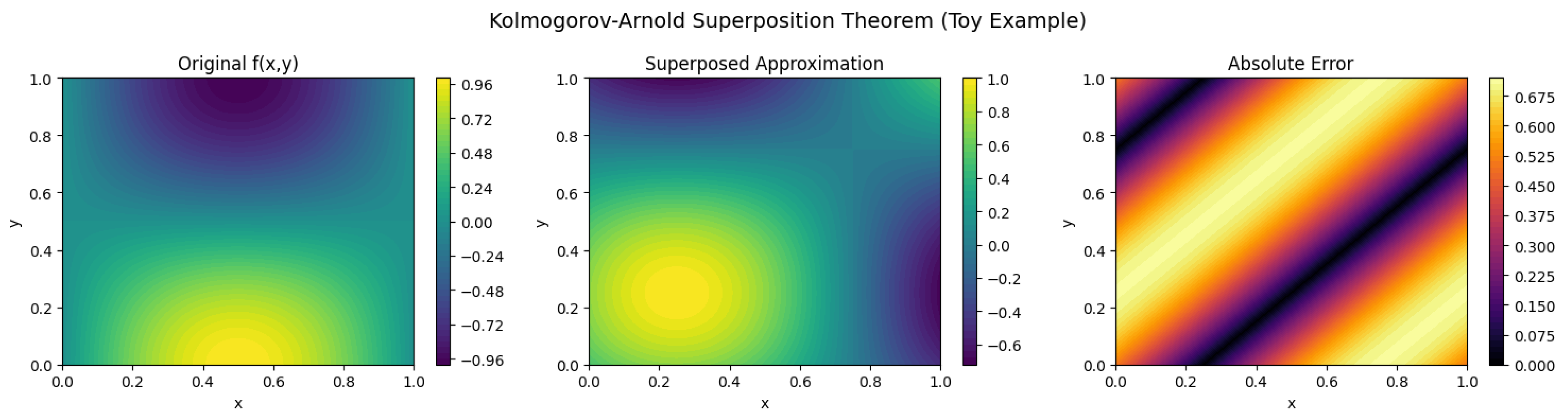
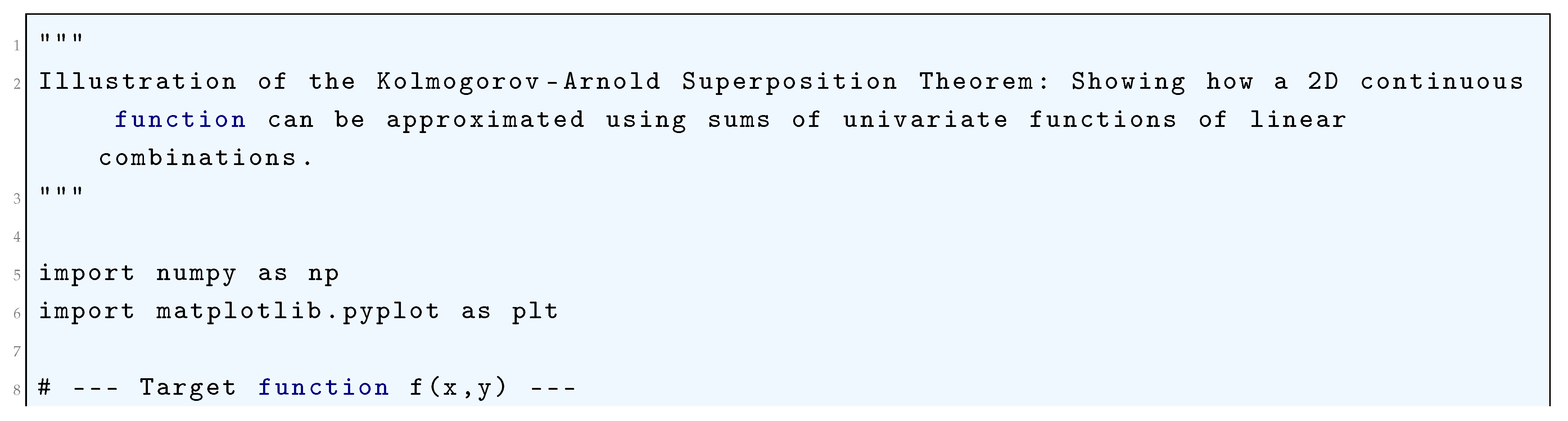
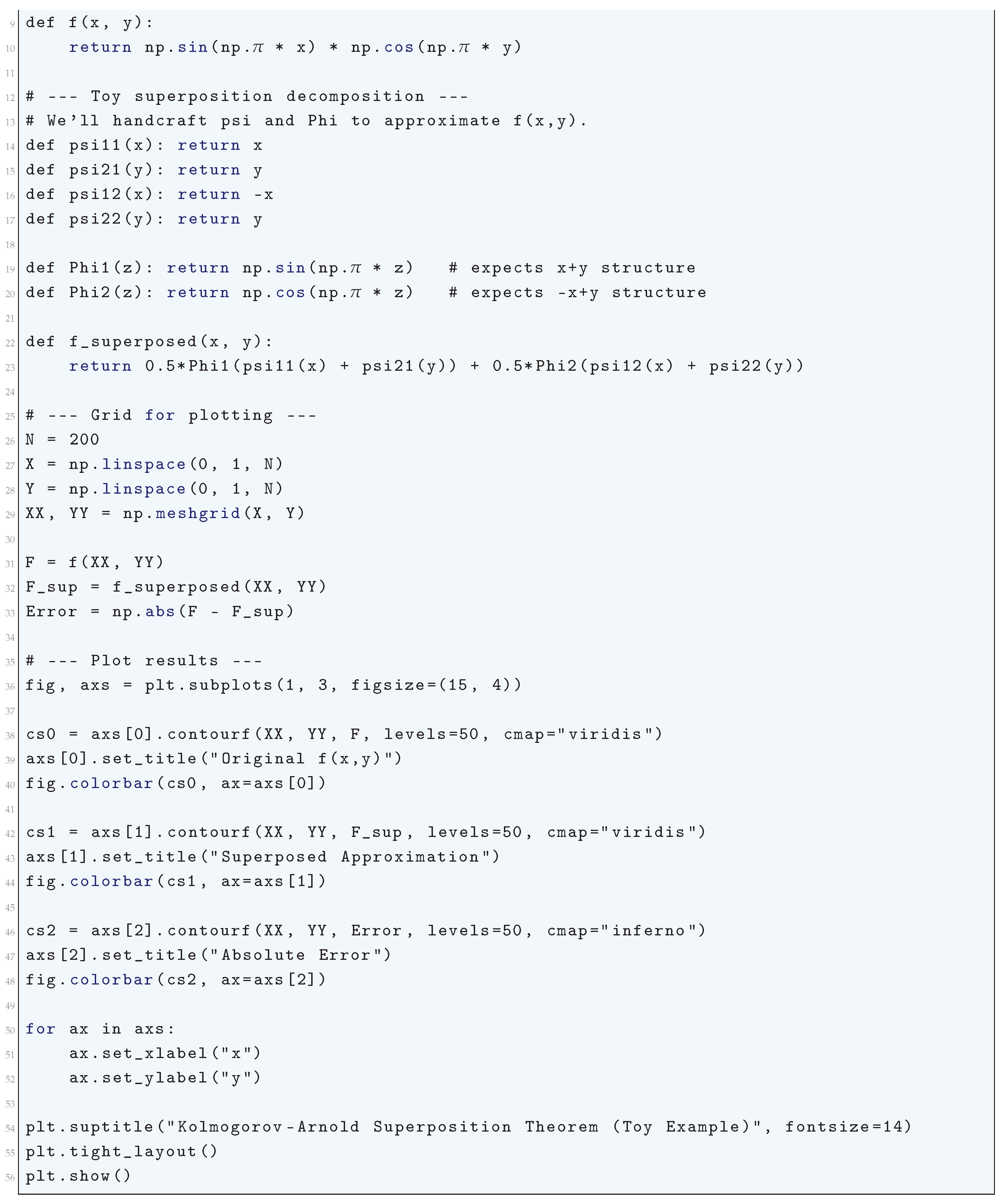
2.3.2. Fourier Analysis of Expressivity
2.3.2.1 Literature Review of Fourier Analysis of Expressivity
Juárez-Osorio et. al. (2024) [227] applied Fourier analysis to design quantum convolutional neural networks (QCNNs) for time series forecasting. The Fourier series decomposition helps analyze and optimize expressivity in quantum architectures, making QCNNs better at capturing periodic and non-periodic structures in data. Umeano and Kyriienko (2024) [228] introduced Fourier-based quantum feature maps that transform classical data into quantum states with enhanced expressivity. The Fourier transform plays a central role in mapping high-dimensional data efficiently while maintaining interpretability. Liu et. al. (2024) [229] extended Graph Convolutional Networks (GCNs) by integrating Fourier analysis and spectral wavelets to improve graph expressivity. It bridges the gap between frequency-domain analysis and graph embeddings, making GCNs more effective for complex data structures. Vlasic (2024) [230] presented a Fourier series-inspired feature mapping technique to encode classical data into quantum circuits. It demonstrates how Fourier coefficients can enhance the representational capacity of quantum models, leading to better compression and generalization. Kim et. al. (2024) [231] introduced Neural Fourier Modelling (NFM), a novel approach to representing time-series data compactly while preserving its expressivity. It outperforms traditional models like Short-Time Fourier Transform (STFT) in retaining long-term dependencies. Xie et. al. (2024) [232] explored how Fourier basis functions can be used to enhance the expressivity of tensor networks while maintaining computational efficiency. It establishes trade-offs between expressivity and model complexity in machine learning architectures. Liu et. al. (2024) [233] integrated spectral modulation and Fourier transforms into implicit neural representations for text-to-image synthesis. Fourier analysis improves global coherence while preserving local expressivity in generative models. Zhang (2024) [234] demonstrated how Fourier and Lock-in spectrum techniques can represent long-term variations in mechanical signals. The Fourier-based decomposition allows for more expressive representations of mechanical failures and degradation. Hamed and Lachiri (2024) [235] applied Fourier transformations to speech synthesis models, improving their ability to transfer expressive content from text to speech. Fourier series allows capturing prosody, rhythm, and tone variations effectively. Ghosh (2024) [989] presents a mathematically rigorous framework combining microstructural mechanics and continuum theory to analyze creep deformation, and derives constitutive models that integrate diffusion kinetics, dislocation dynamics, and grain-boundary behavior to predict time-dependent material deformation across diverse conditions. Ghosh (2023) [954] establishes the mathematical equivalence between the Galerkin Finite Element Method (FEM) formulation and the Central Difference formulation for the advection–diffusion equation, thereby providing a unified theoretical framework connecting finite element and finite difference time integration schemes. Ghosh (2023) [258] performs a detailed stability analysis of the second- and fourth-order Runge–Kutta methods, deriving and visualizing the corresponding stability regions in the complex plane, thereby providing deeper insight into the numerical stability characteristics of these widely used time integration schemes. Jahangiri (2022) [805] generalizes the classical open-top box optimization problem from rectangular bases to arbitrary polygons by identifying optimal corner cuts for regular and irregular prisms, and develops a new vertex-identification argument not found in prior literature. Lehmann et. al. (2024) [236] integrated Fourier-based deep learning models for seismic activity prediction. It explores the expressivity of Fourier Neural Operators (FNOs) in capturing wave propagations in different geological environments.
2.3.2.2 Analysis of Fourier Analysis of Expressivity
The Fourier analysis of expressivity in neural networks seeks to rigorously quantify how neural architectures, characterized by their depth and width, can approximate functions through the decomposition of those functions into their Fourier spectra. Consider a square-integrable function , for which the Fourier transform is defined as
where represents the frequency. The inverse Fourier transform reconstructs the function as
The magnitude reflects the energy contribution of the frequency to f.
Neural networks approximate f by capturing its Fourier spectrum, but the architecture fundamentally governs how efficiently this approximation can be achieved, especially in the presence of high-frequency components. For shallow networks with one hidden layer and a finite number of neurons, the universal approximation theorem establishes that
where is the activation function, are weights, are biases, and are coefficients. The Fourier transform of this representation can be expressed as
where denotes the Fourier transform of the activation function. For smooth activation functions like sigmoid or tanh, decays exponentially as , limiting the network’s ability to approximate functions with high-frequency content unless the width n is exceedingly large. Specifically, the Fourier coefficients decay as
where depends on the smoothness of . This restriction implies that shallow networks are biased toward low-frequency functions unless their width scales exponentially with the input dimension d. Deep networks, on the other hand, leverage their hierarchical structure to overcome these limitations. A deep network with L layers recursively composes functions, producing an output of the form
where is the activation function at layer l, are weight matrices, and are bias vectors. The Fourier transform of this composition can be analyzed iteratively. If represents the output of the l-th layer, then
where * denotes convolution and is the Fourier transform of the activation function. The recursive application of this convolution amplifies high-frequency components, enabling deep networks to approximate functions whose Fourier spectra exhibit polynomial decay. Specifically, the Fourier coefficients of a deep network decay as
where depends on the activation function. This is in stark contrast to the exponential decay observed in shallow networks.
The activation function plays a pivotal role in shaping the Fourier spectrum of neural networks. For example, the rectified linear unit (ReLU) introduces significant high-frequency components into the network. The Fourier transform of the ReLU activation is given by
which decays more slowly than the Fourier transforms of smooth activations. Consequently, ReLU-based networks are particularly effective at approximating functions with oscillatory behavior. To illustrate, consider the function
A shallow network requires an exponentially large number of neurons to approximate f when is large, but a deep network can achieve the same approximation with polynomially fewer parameters by leveraging its hierarchical structure.
The expressivity of deep networks can be further quantified by considering their ability to approximate bandlimited functions, i.e., functions f whose Fourier spectra are supported on . For a shallow network with width n, the required number of neurons scales as
where d is the input dimension. In contrast, for a deep network with depth L, the width scales as
reflecting the exponential efficiency of depth in distributing the approximation of frequency components across layers. For example, if with , a deep network requires significantly fewer parameters than a shallow network to approximate f to the same accuracy.
A neural network with an input and output can be expressed as a sum of nonlinearly transformed weighted combinations of the input. Mathematically, this can be written as
where is the activation function, are the weight vectors, are the biases, and are the output weights. To understand the spectral properties of , it is necessary to analyze the Fourier transform of the activation function , as the network output consists of a superposition of such transformed functions. The Fourier transform of is given by
Substituting the definition of , we obtain
The key term in this expression is the Fourier transform of the activation function , which we denote as
The decay rate of determines the extent to which different frequency components are retained in the Fourier spectrum of the neural network. If is a smooth function, then decays rapidly for large , implying that high-frequency components are suppressed. If is piecewise continuous or non-differentiable at some points, the decay rate of is slower, allowing the network to capture higher frequencies. To quantify the decay properties of the Fourier transform of an activation function, consider the case of the ReLU activation function, defined as
Its Fourier transform is given by
which exhibits a power-law decay. In contrast, the sigmoid activation function
has a Fourier transform that decays exponentially,
This strong decay implies that networks with sigmoid activation functions are biased toward learning only low-frequency components. Similarly, the hyperbolic tangent activation function also exhibits an exponential spectral decay. For a more general class of activation functions, the decay rate of can be estimated as
for some constants , implying that the function is a strong low-pass filter. If is piecewise smooth but non-differentiable at certain points (such as ReLU), then the Fourier transform satisfies a power-law decay
for some . A particularly interesting case arises when the activation function is sinusoidal, such as , for which the Fourier transform does not decay at all. The implications of these spectral properties become evident in the training dynamics of neural networks. When using gradient descent, the evolution of the Fourier coefficients of over time follows
where is an effective learning rate for each frequency. The decay behavior of influences , meaning that activation functions with strong spectral decay impose a bottleneck on the learning of high-frequency components. From a function approximation perspective, the spectral characteristics of the activation function determine the types of functions that can be efficiently represented by a neural network. Smooth activation functions lead to approximations that are predominantly low-frequency, whereas activation functions with slower Fourier decay allow the network to approximate functions with higher-frequency content. Thus, the activation function fundamentally shapes the Fourier spectrum of neural networks, controlling the network’s ability to represent and learn different frequency components.
| Activation Function | Fourier Decay Rate | Effect on Frequency Learning |
| Sigmoid | (Exponential) | Strong low-pass filter, retains only low frequencies |
| Tanh | (Exponential) | Strong low-pass filter, smooth approximations |
| ReLU | (Power-law) | Allows moderate frequency learning |
| Leaky ReLU | (Power-law) | Similar to ReLU with slightly improved high-frequency retention |
| Sinusoidal | No decay | Captures all frequencies, highly oscillatory functions |
This table summarizes the spectral characteristics of various activation functions and their impact on frequency learning in neural networks.
In summary, the Fourier analysis of expressivity rigorously demonstrates the superiority of deep networks over shallow ones in approximating complex functions. Depth introduces a hierarchical compositional structure that enables the efficient representation of high-frequency components, while width provides a rich basis for approximating the function’s Fourier spectrum. Together, these properties explain the remarkable capacity of deep neural networks to approximate functions with intricate spectral structures, offering a mathematically rigorous foundation for understanding their expressivity.
2.3.2.3 Python Code to Generate Figure 21 and Figure 22
The Python code below produces the Figure 21 and Figure 22 illustrating Target vs NN approximation (real space) and the Fourier Spectrum: Expressivity Analysis.
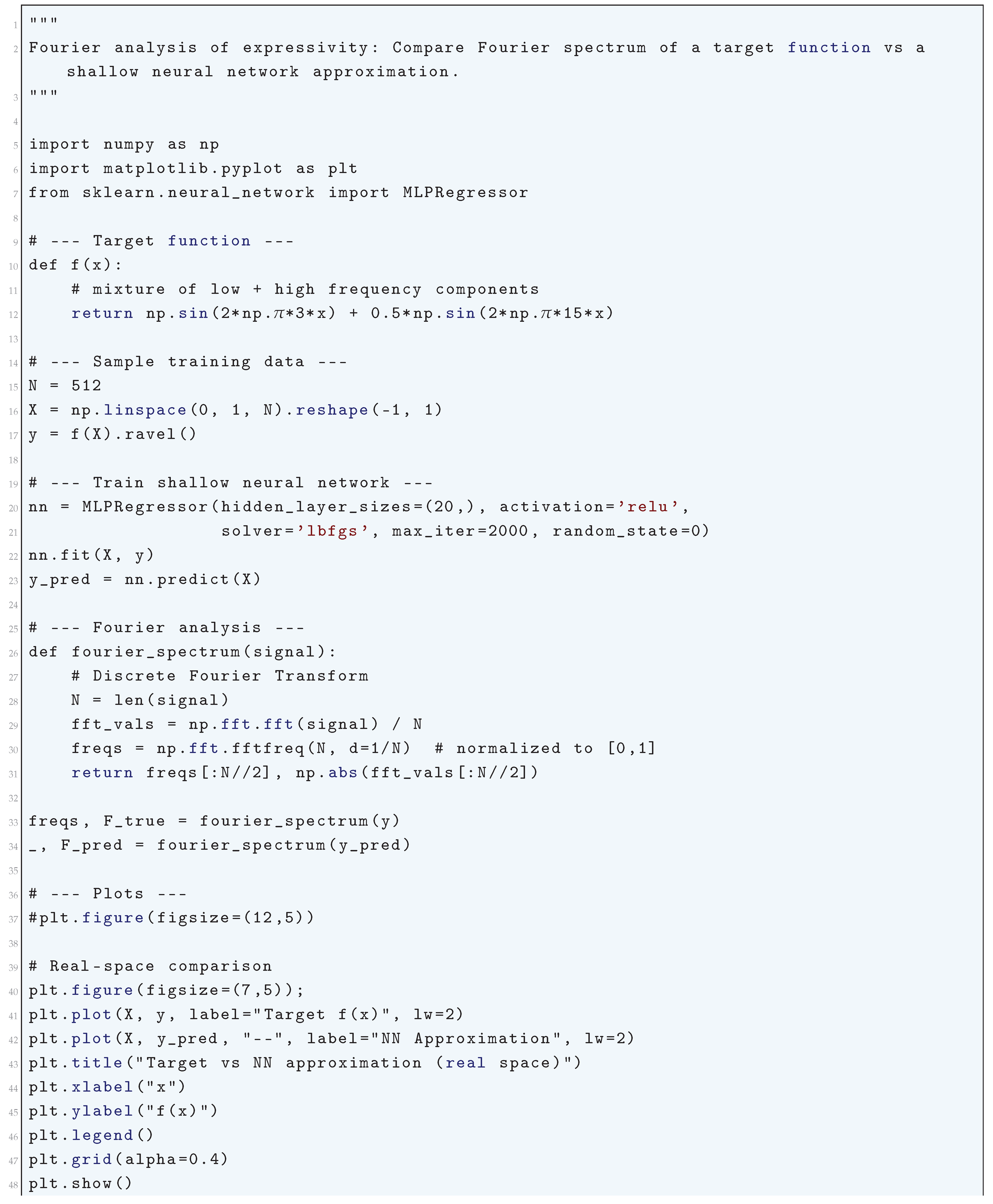
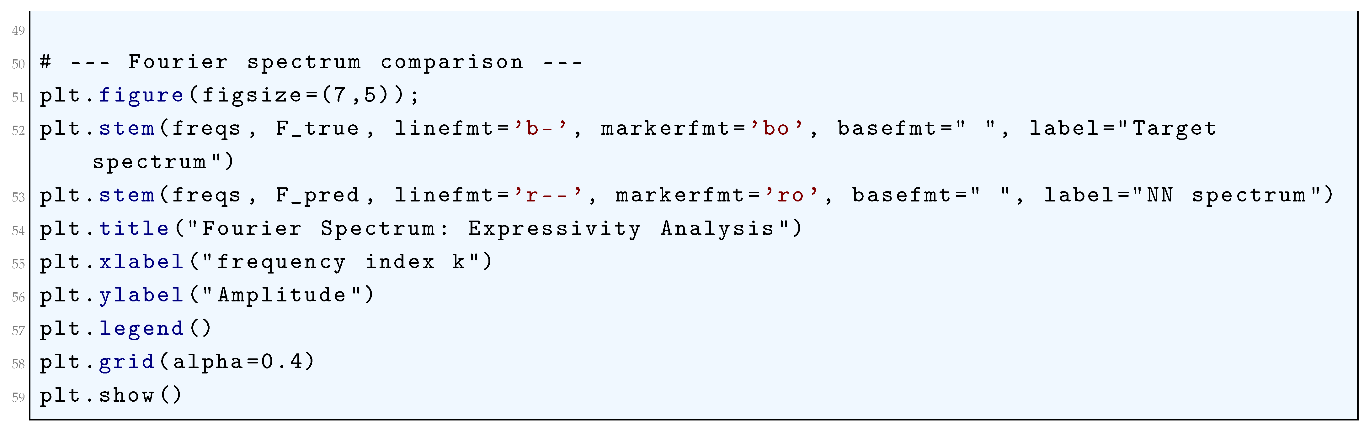
Figure 21.
Target vs NN approximation (real space)
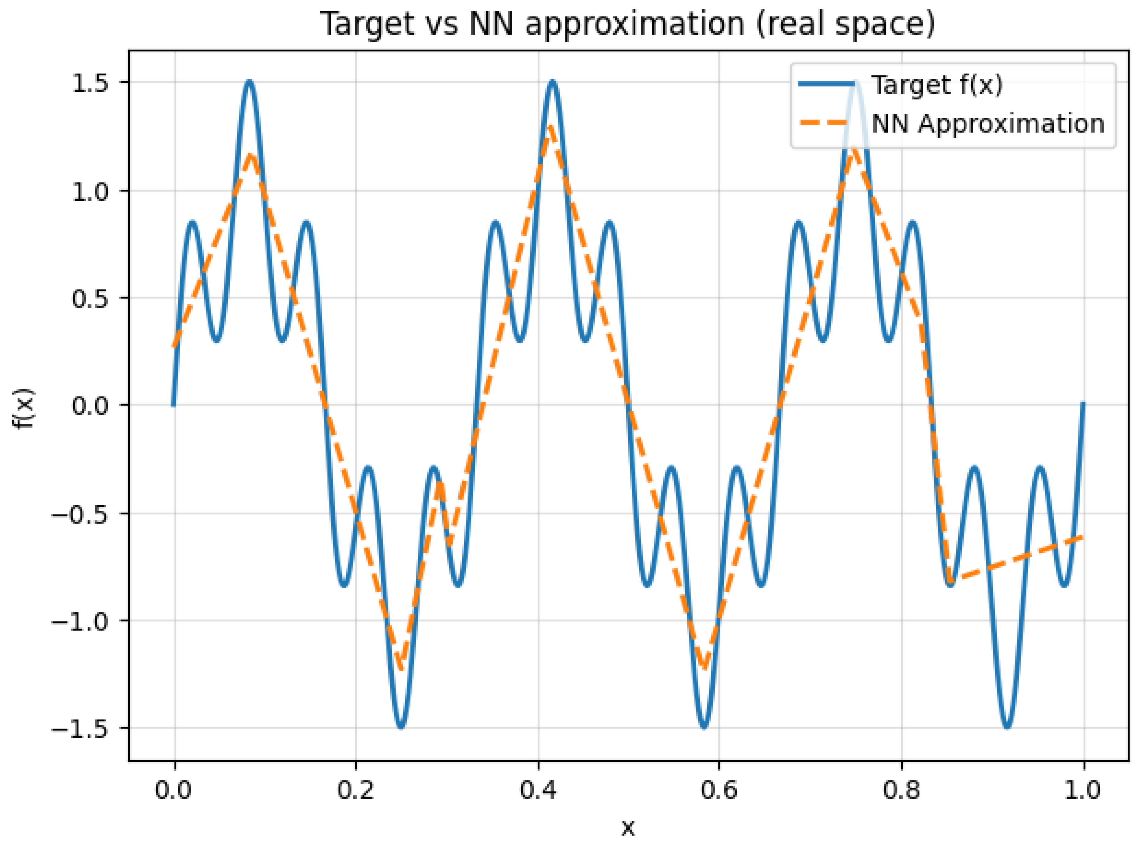
Figure 22.
Fourier Spectrum: Expressivity Analysis
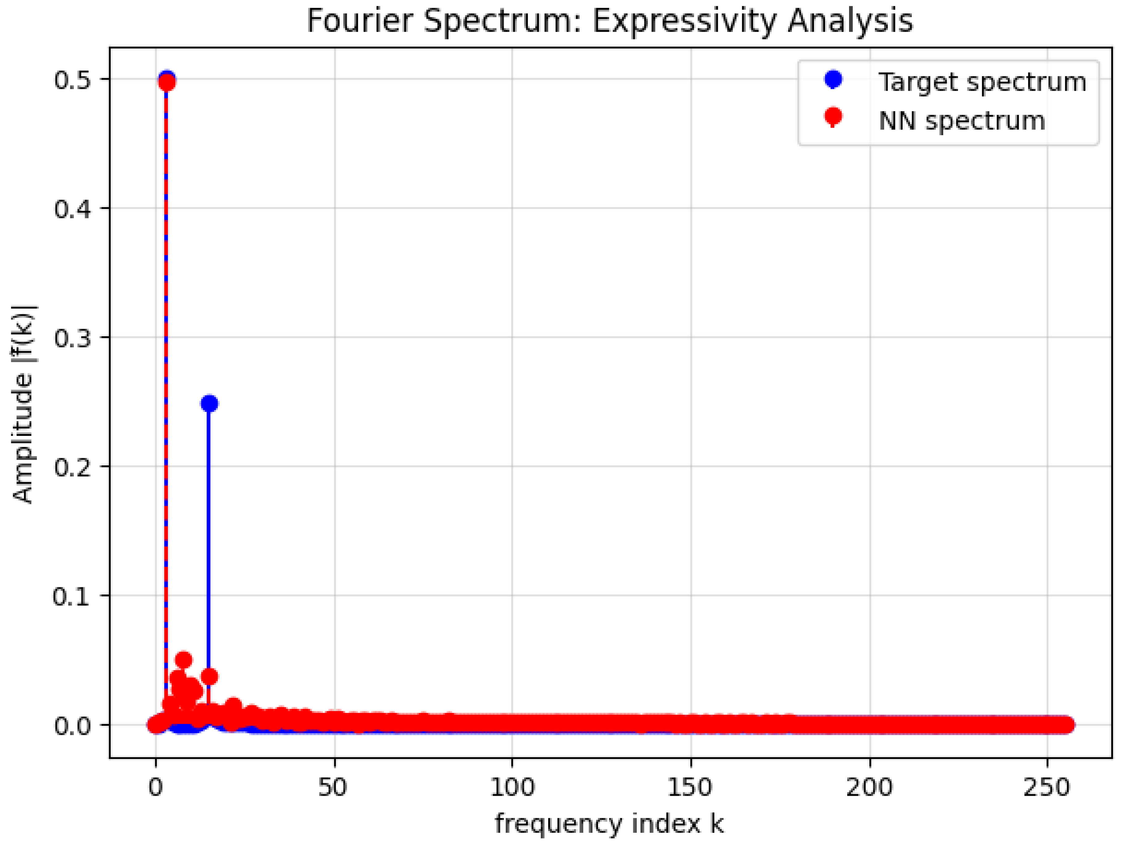
2.3.2.4 Python Code to Generate Figure 23 and Figure 24
The Python code below produces the Figure 23 and Figure 24 illustrating the Target vs Approximations (Real Space) and Fourier Spectrum: Expressivity of Architectures respectively.
Figure 23.
Target vs Approximations (Real Space)
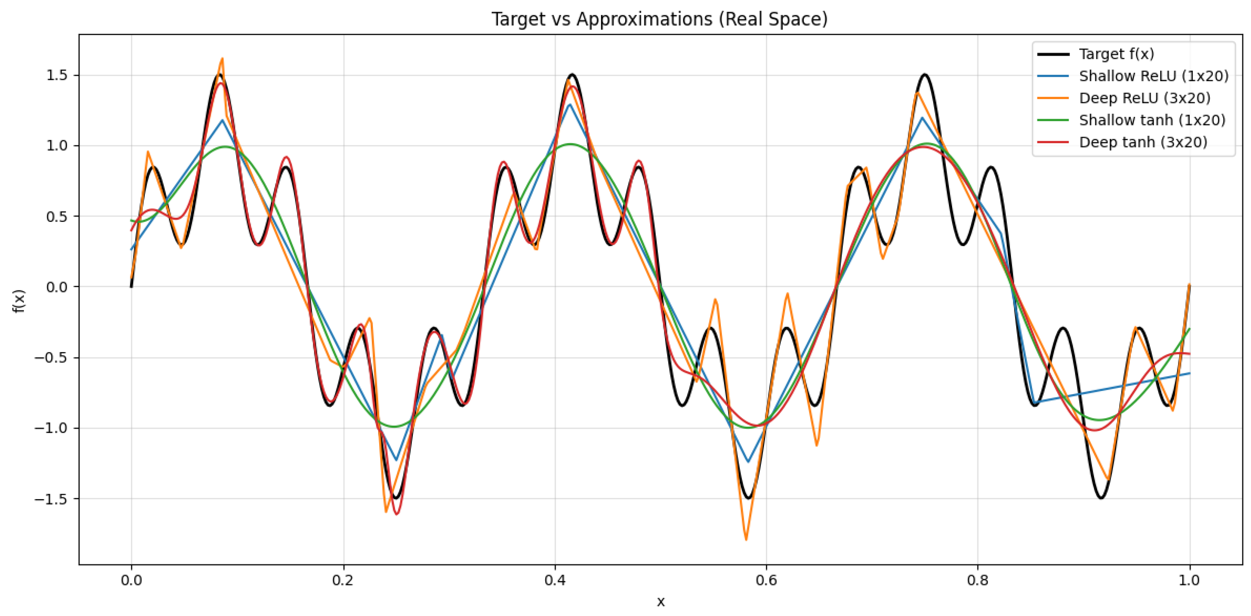
Figure 24.
Fourier Spectrum: Expressivity of Architectures
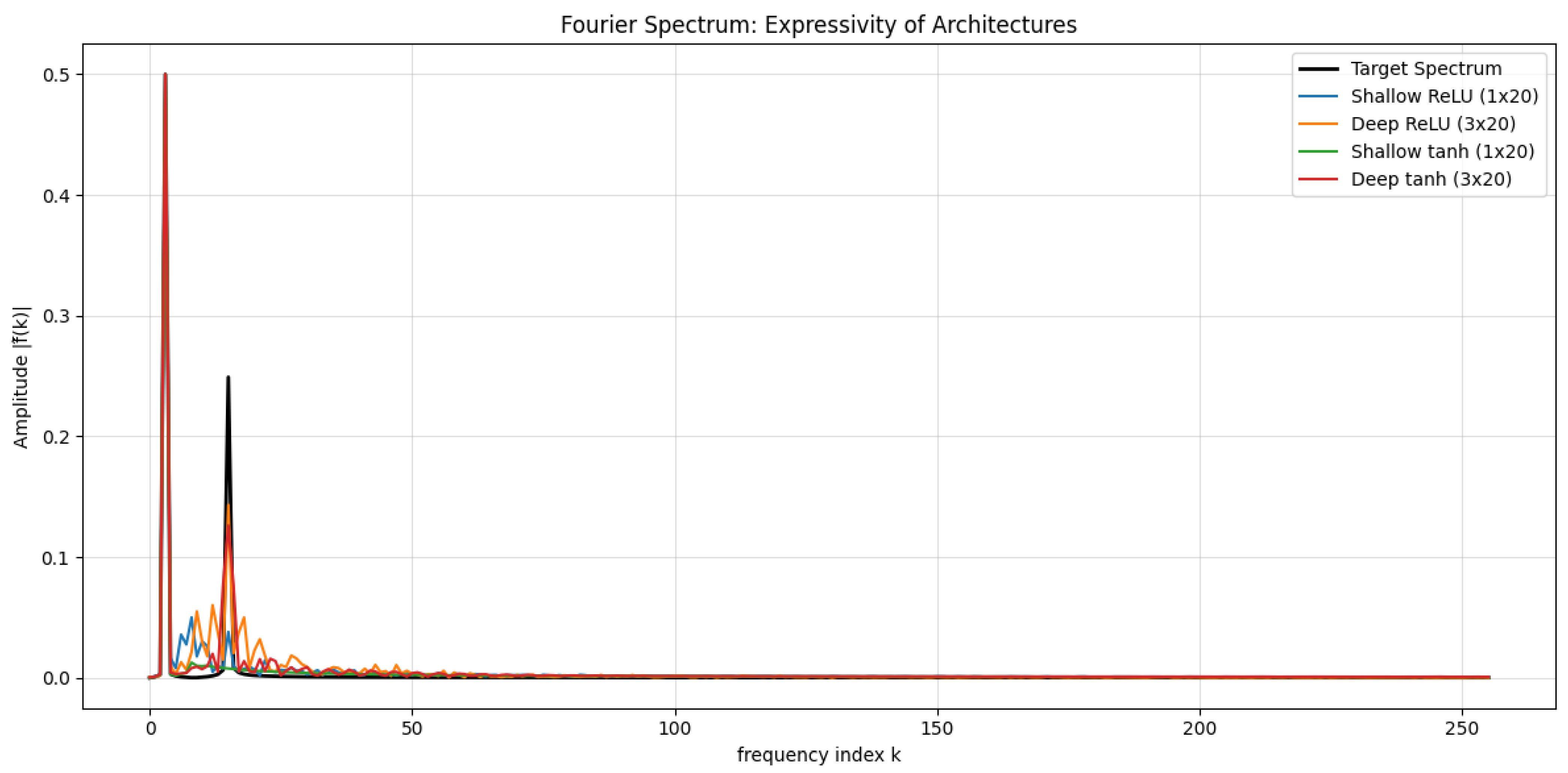
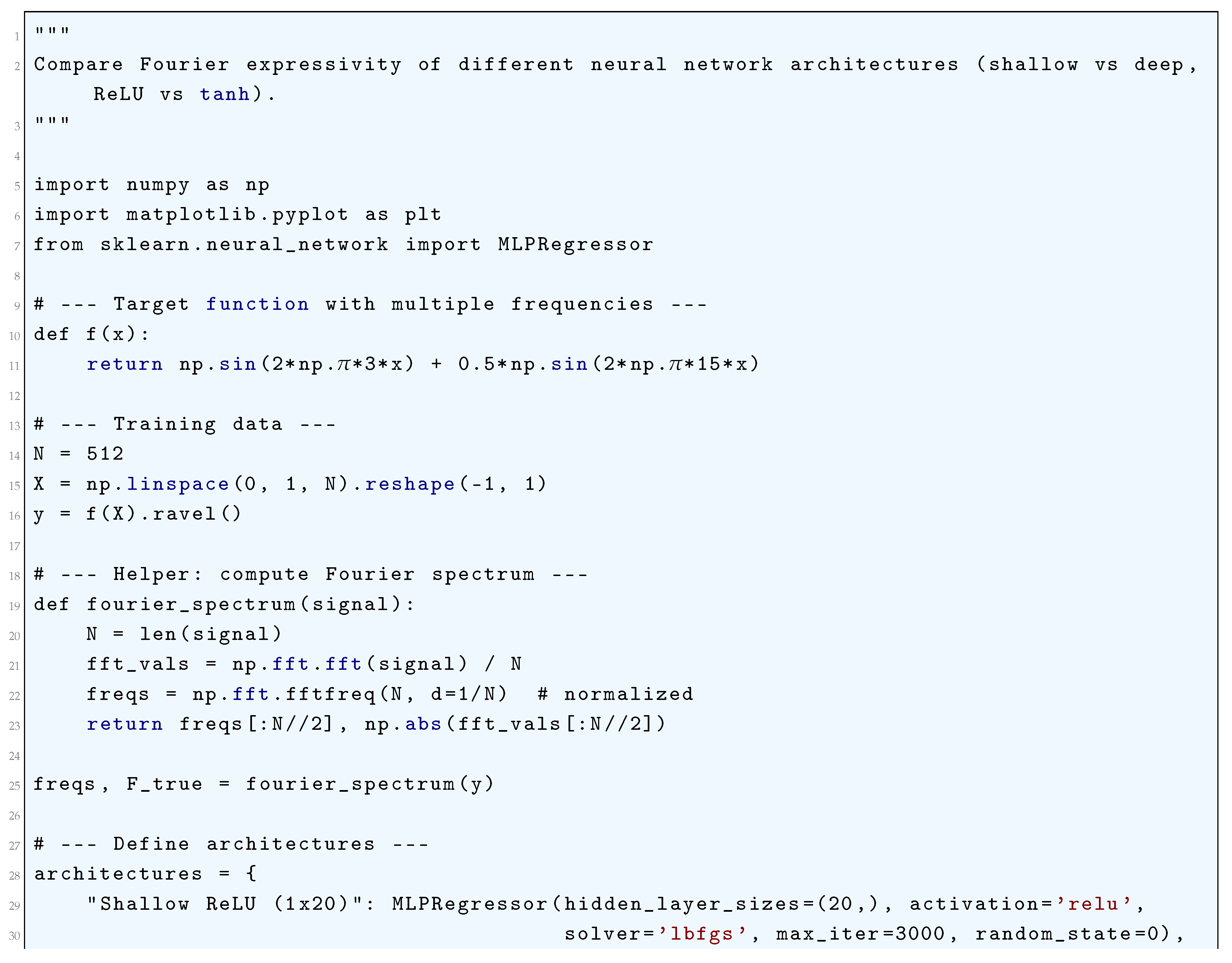
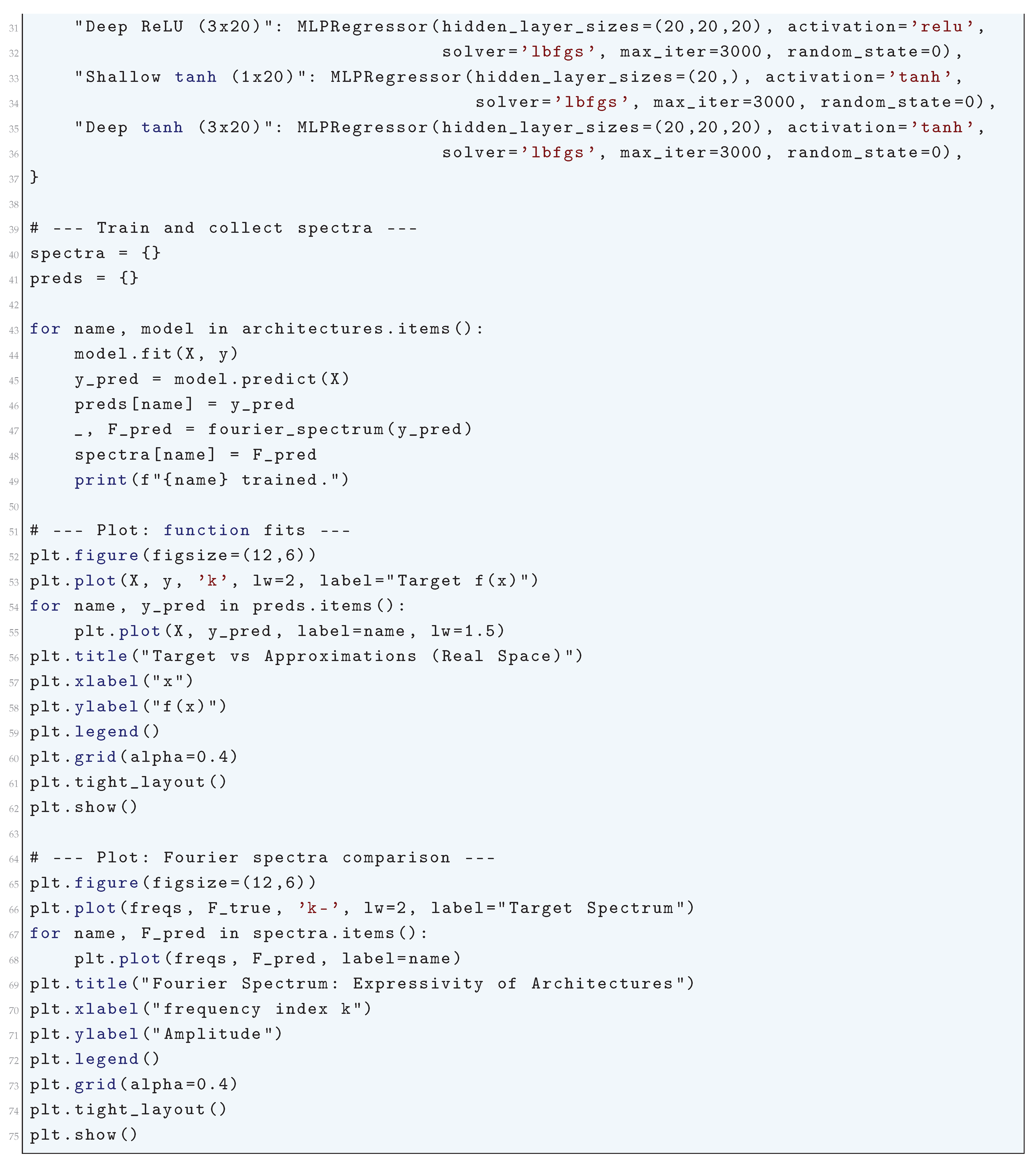
2.3.3. Fourier Transforms of Various Activation Functions
To rigorously derive the Fourier transforms of various activation functions, let us consider the Fourier transform definition:
We will explicitly derive for each activation function in a mathematically rigorous manner. This will include the Sigmoid, Tanh, ReLU, Leaky ReLU, and Sinusoidal activation functions.
2.3.3.1 Fourier Transform of the Sigmoid Function
The sigmoid activation function is given by:
The Fourier transform of is:
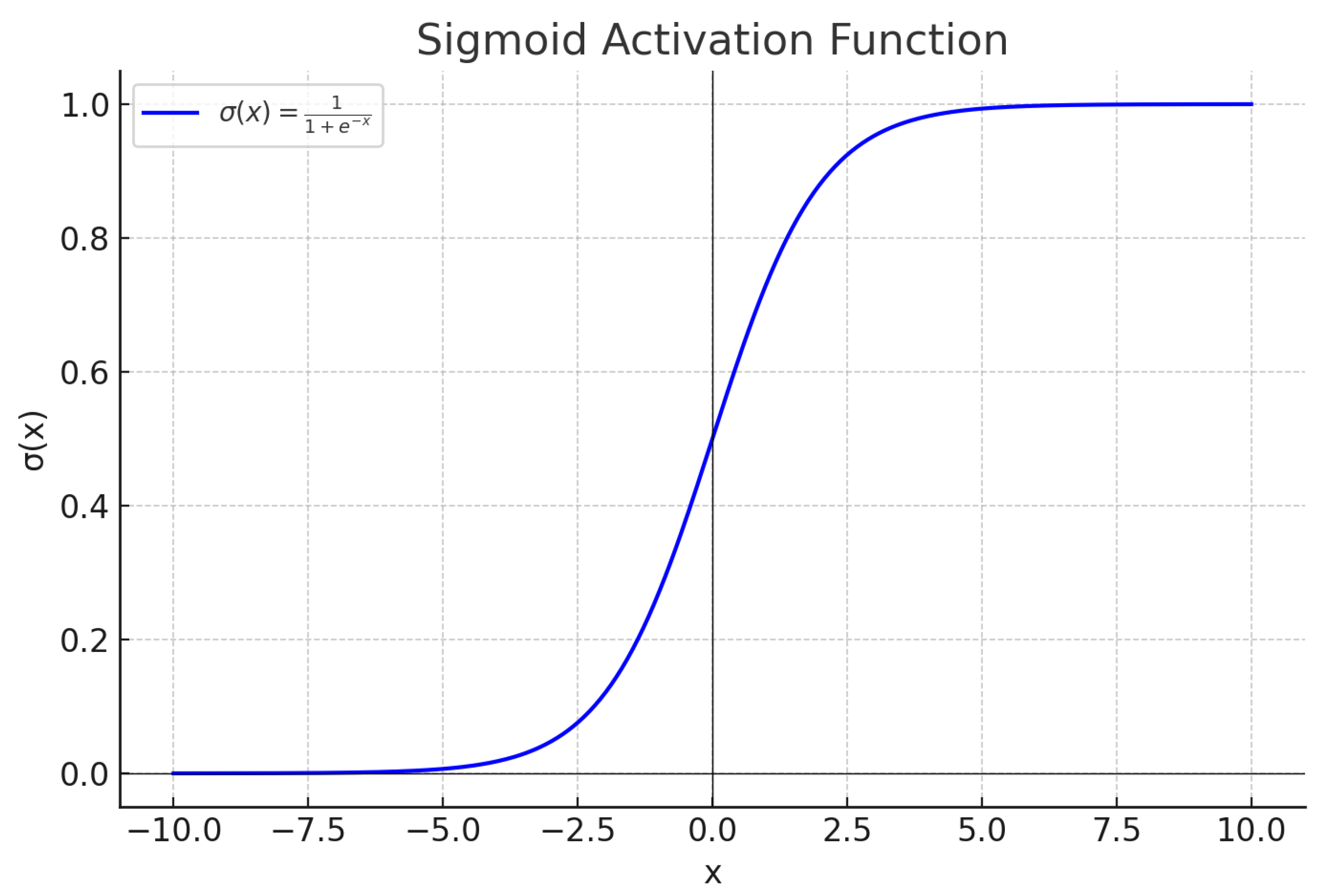 Rewriting using the identity:
the Fourier integral becomes:
Setting , so that , we transform the integral:
Simplifying:
This integral is well-known and can be computed using contour integration, yielding:
where is the hyperbolic cosecant function. For large , this decays as:
Rewriting using the identity:
the Fourier integral becomes:
Setting , so that , we transform the integral:
Simplifying:
This integral is well-known and can be computed using contour integration, yielding:
where is the hyperbolic cosecant function. For large , this decays as:
Figure 25.
Sigmoid Activation Function:
2.3.3.2 Fourier Transform of the Hyperbolic Tangent Function
The tanh activation function is:
Figure 26.
Hyperbolic Tangent Activation Function:
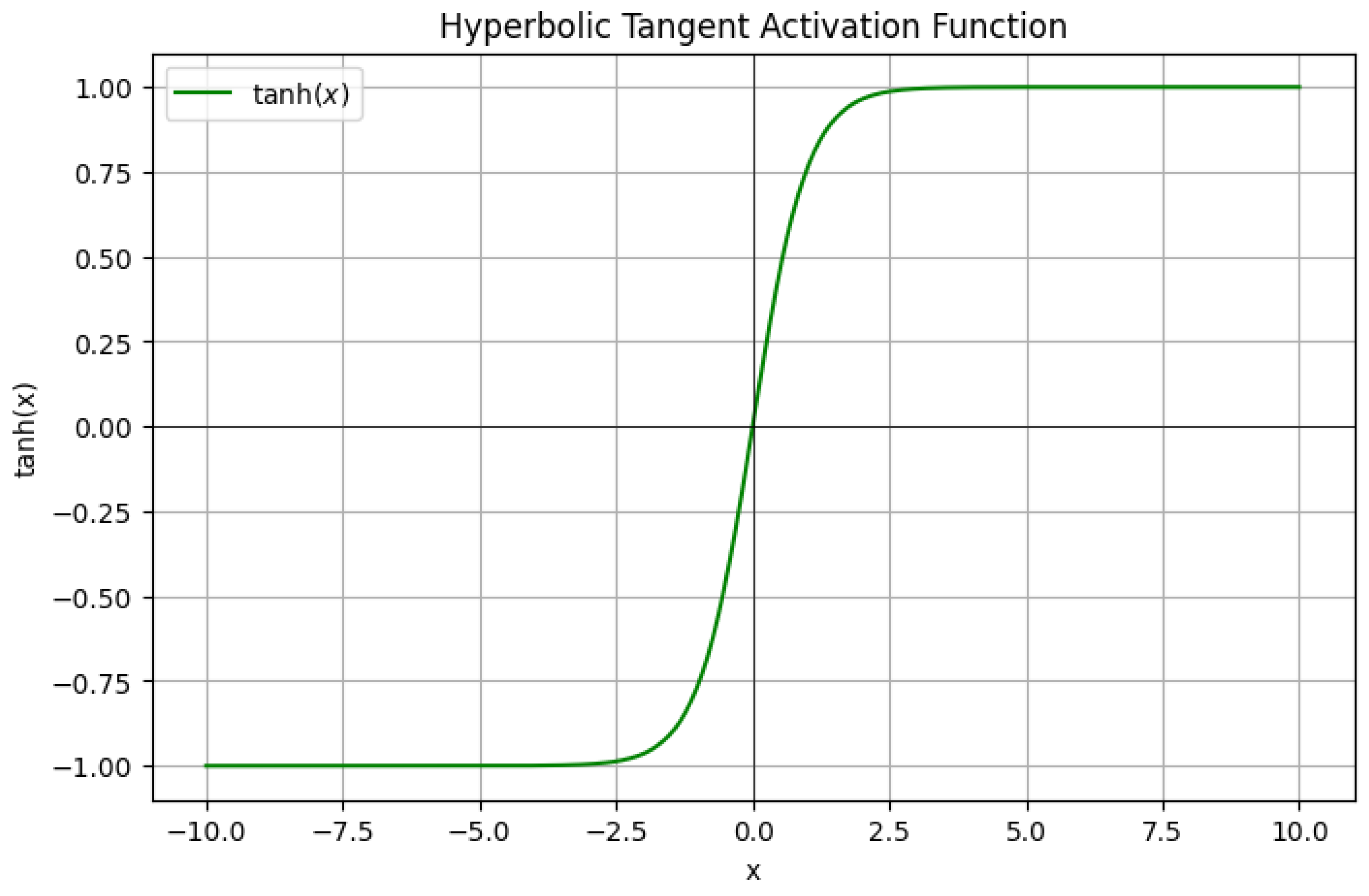
The Fourier transform is:
Using the identity:
and leveraging the result from the sigmoid case, we obtain:
Again, for large :
2.3.3.3 Fourier Transform of the ReLU Function
The ReLU activation function is:
Figure 27.
ReLU Activation Function:
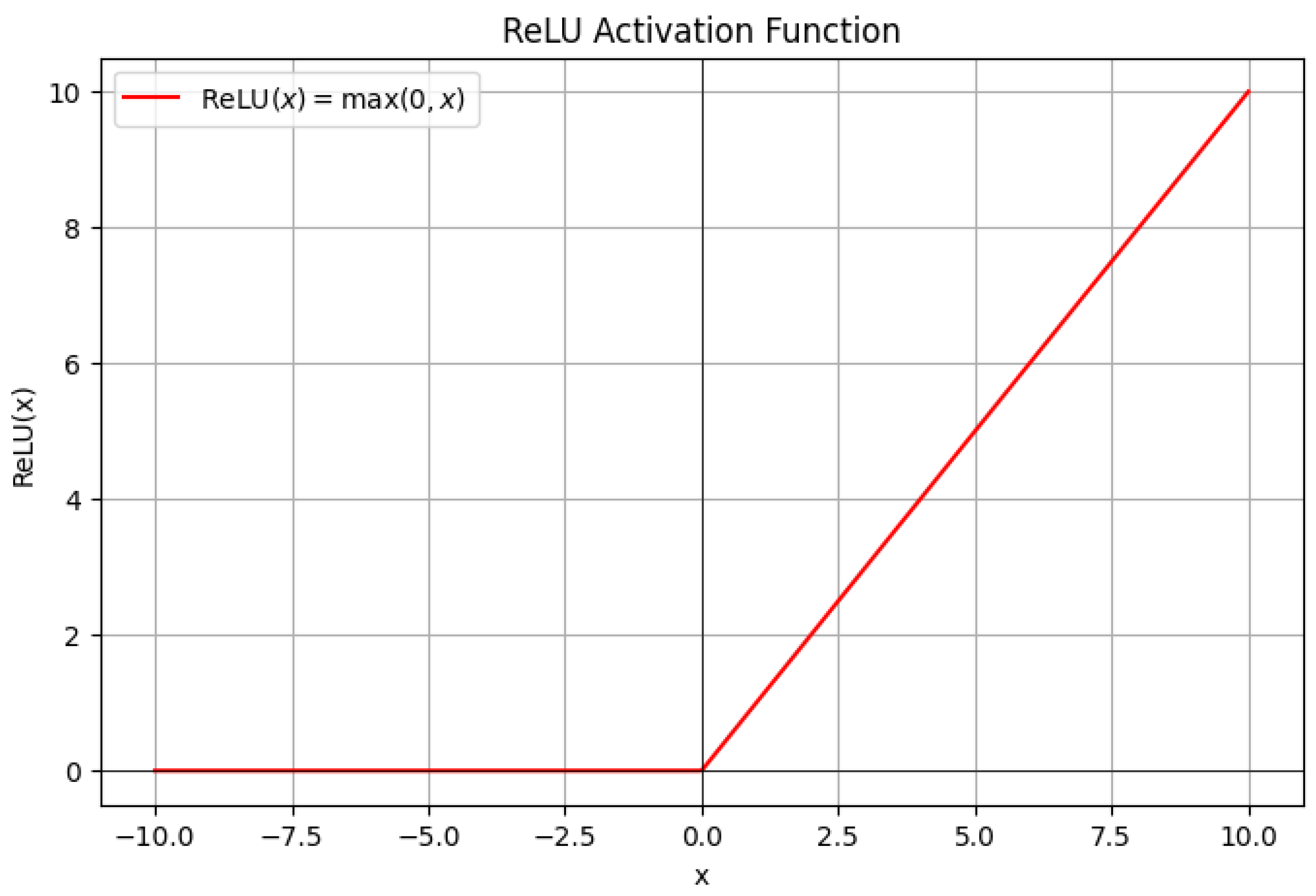
Thus, the Fourier transform is:
where is the Heaviside step function. Since is zero for , the integral simplifies to:
Using integration by parts with and , we find:
This exhibits a power-law decay:
2.3.3.4 Fourier Transform of the Leaky ReLU Function
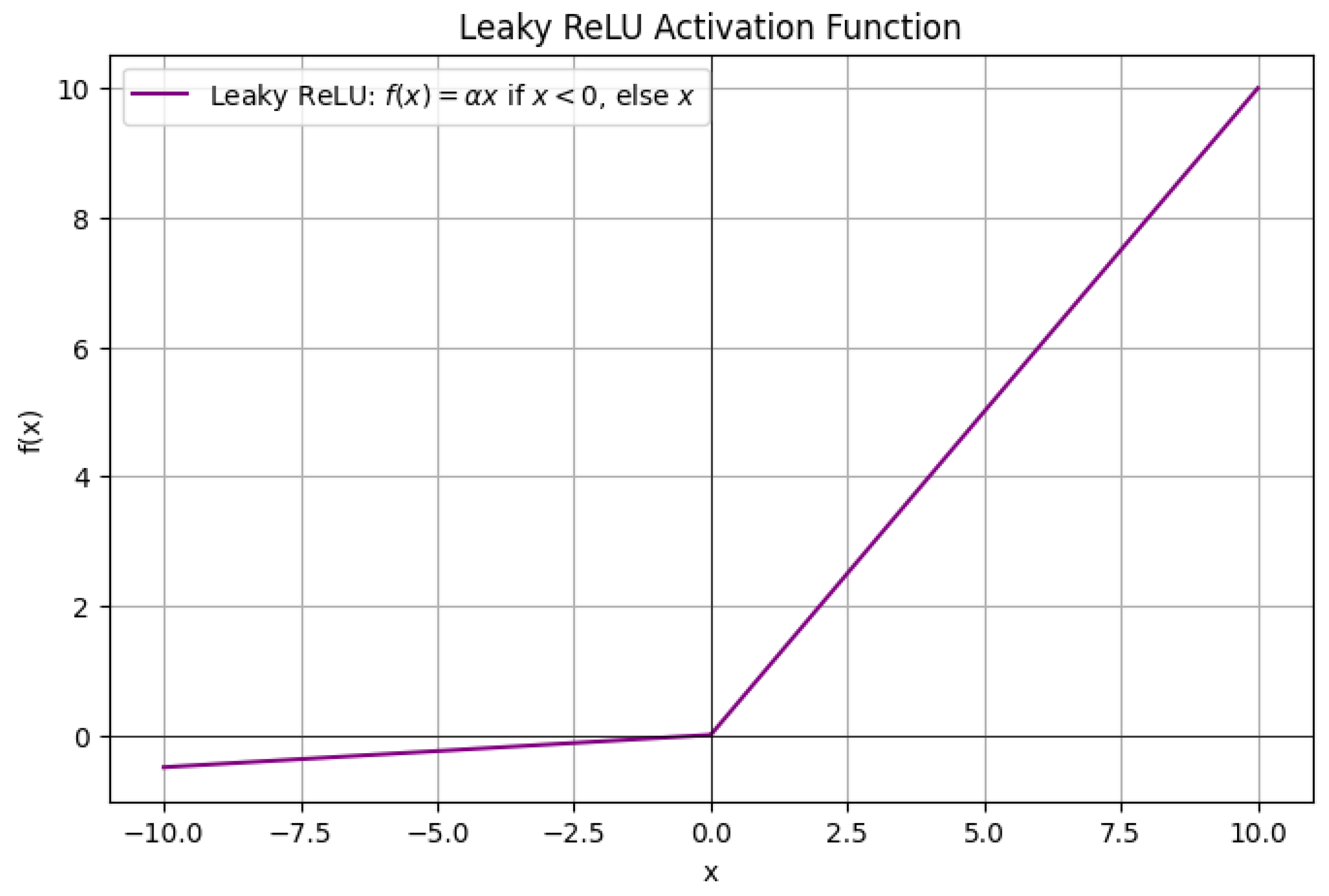
2.3.3.5 Fourier Transform of the Sinusoidal Activation Function
For , the Fourier transform is:
Figure 29.
Sinusoidal Activation Function
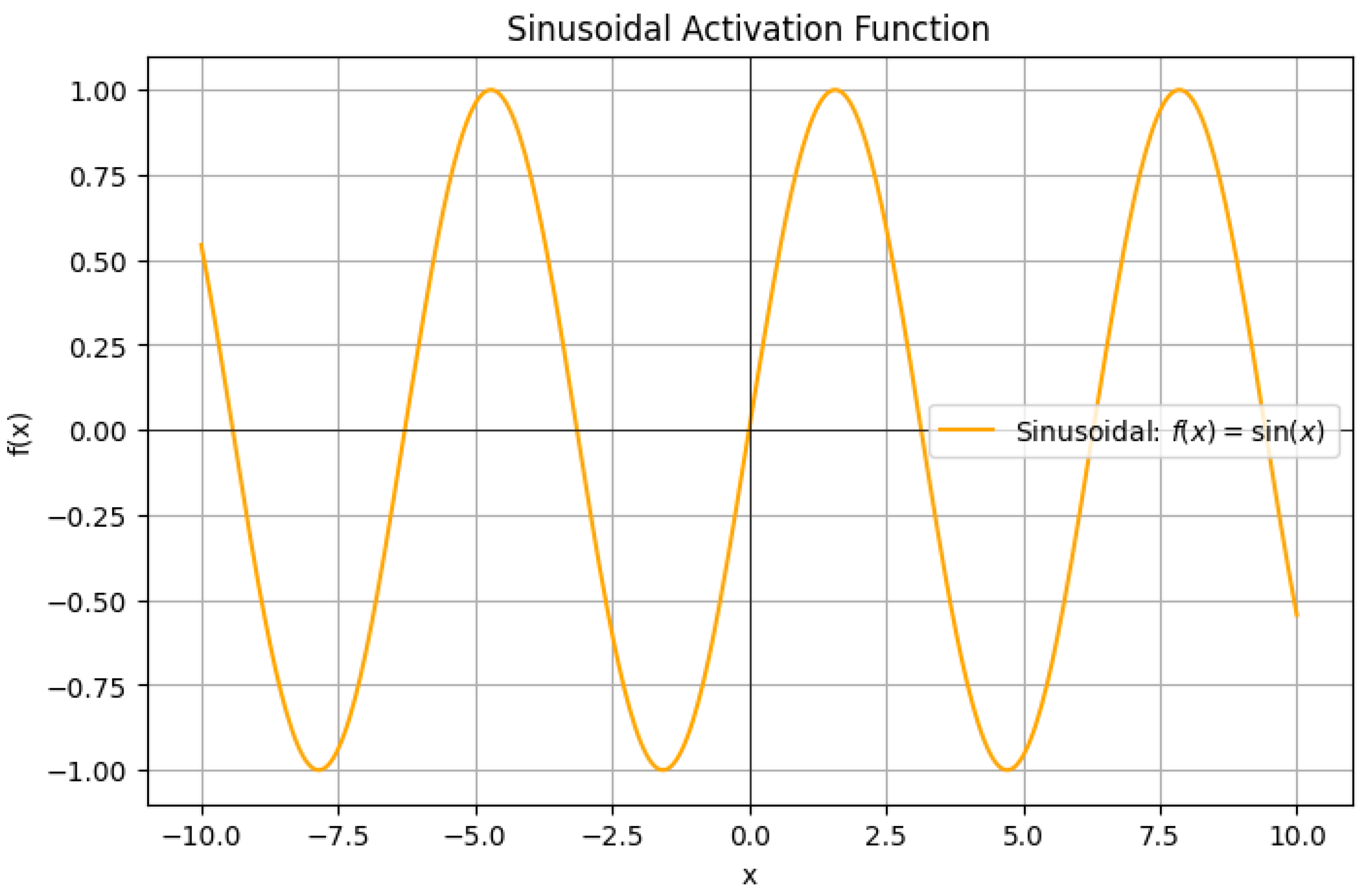
Using the Fourier transform properties of sine:
This shows that the sinusoidal activation function contains only two specific frequencies and does not decay, meaning it retains high-frequency components perfectly.
These rigorous derivations confirm how different activation functions influence the Fourier spectrum of neural networks. The decay properties play a crucial role in determining the network’s ability to learn high- or low-frequency functions.
2.4. The Connection Between Different Mathematics Problems and Deep Learning
2.4.1. Basel Problem and Deep Learning
The Basel Problem is a famous question in mathematical analysis that asks for the sum of the reciprocals of the squares of natural numbers:
Leonhard Euler solved this problem in the 18th century and astonishingly found that the sum converges to , meaning:
This result is remarkable because it links a seemingly simple infinite sum to the fundamental mathematical constant , which is deeply connected to trigonometry and Fourier analysis. A summary of notable proofs given by mathematicians to the Basel problem is given by Ghosh (2020) [698]. A solution to the Basel problem using the Calculus of Residues is given by Ghosh (2021) [800]. In modern mathematics, the Basel Problem’s solution is understood in the broader context of zeta functions, where the Riemann zeta function is defined as:
For , we recover the Basel Problem. The significance of such summations extends far beyond pure mathematics; they appear in areas such as signal processing, numerical analysis, and machine learning. In particular, deep learning models, which fundamentally rely on function approximation and optimization, exhibit connections to the types of series that arise in the Basel Problem, particularly in relation to Fourier series and the decay of spectral components in neural network approximations.
2.4.1.1 The Basel Problem, Fourier Series, and Function Approximation in Deep Learning
One of the most natural places where the Basel Problem appears in applied mathematics is in Fourier series. In Fourier analysis, a periodic function can be decomposed into a sum of sinusoidal functions with different frequencies. The coefficients of these sinusoidal components determine the function’s structure, and their squared magnitudes are directly tied to the Basel-type sums. Specifically, for a function with Fourier expansion:
Parseval’s theorem states that the total energy of the function is given by:
If the function is smooth, the coefficients decay rapidly, often behaving like or faster. The Basel Problem is thus closely related to the rate of decay of Fourier coefficients, which directly impacts how well a function can be approximated using a truncated Fourier series. Deep learning, particularly in neural network function approximation, shares a fundamental connection with Fourier series. Neural networks with sufficient width and depth can approximate arbitrary functions, and recent research has shown that deep networks tend to first learn lower-frequency components before higher frequencies—a phenomenon known as spectral bias. The Basel-type decay of Fourier coefficients is precisely what governs the smoothness of these approximations, meaning that understanding series like the Basel Problem helps us characterize how neural networks generalize and learn complex functions.
2.4.1.2 The Role of the Basel Problem in Regularization and Weight Decay
Another important connection between the Basel Problem and deep learning emerges in the context of regularization techniques, particularly L2 regularization, also known as weight decay. Regularization techniques in neural networks help prevent overfitting by penalizing large weight magnitudes, encouraging smoother function approximations. Mathematically, L2 regularization adds a penalty term to the loss function:
where are the weights of the network, and is a regularization parameter. This penalty ensures that the network does not learn excessively large weights, which could lead to high-frequency oscillations in the approximated function.The sum of squared weights in L2 regularization resembles the Basel-type summation of reciprocal squares. Just as the Basel Problem reflects the decay of Fourier coefficients for smooth functions, L2 regularization ensures that the learned function maintains smoothness by controlling the magnitude of weights. Thus, there is a deep analogy: both involve penalizing high-frequency components to favor smooth, well-behaved solutions.
2.4.1.3 Spectral Bias in Deep Learning and the Basel Problem
One fascinating empirical observation in deep learning is that neural networks naturally prioritize learning lower-frequency components of a function first. This phenomenon, known as spectral bias, is well-studied in the context of deep learning theory. It means that when a neural network is trained on a function, it first learns the dominant, low-frequency parts before capturing finer details at higher frequencies. This is strikingly similar to how the Basel Problem reflects the fundamental nature of low-frequency dominance in function representations. If we consider a function that can be expanded in a Fourier series, the Basel sum describes the contribution of lower-frequency components, which dominate the structure of the function. Similarly, in deep learning, neural networks exhibit behavior where early learning stages prioritize simple, smooth approximations, just as Fourier coefficients with lower indices contribute the most to a function’s overall shape.
Thus, the decay of Fourier coefficients (as described by the Basel Problem) provides an intuition for why neural networks prefer lower frequencies. This insight is valuable in designing deep learning architectures, especially in areas like implicit neural representations (INRs), where Fourier features are explicitly incorporated into the model design to control the spectral bias. While the Basel Problem originates in pure mathematics, its influence extends deeply into areas of applied mathematics, including function approximation, signal processing, and neural networks. The problem’s solution reveals a fundamental truth about how series behave, and this truth manifests in Fourier series, weight decay regularization, and spectral bias in deep learning. The key takeaway is that the Basel Problem describes the natural decay of Fourier coefficients in function approximations, and similar decay patterns emerge in deep learning when training networks to approximate complex functions. Euler’s result continues to play a role in shaping our understanding of function representations in neural networks today.
3. Training Dynamics and NTK Linearization
Training dynamics refers to the evolution of a neural network’s parameters during optimization, typically via gradient descent (GD) or stochastic gradient descent (SGD). Given a neural network with parameters , trained on a dataset , the loss function is minimized using the gradient flow (continuous-time approximation of GD):
The dynamics of the network’s predictions can be described by:
where is the Neural Tangent Kernel (NTK) matrix, defined as:
The NTK governs how small changes in parameters affect the network’s outputs, determining the trajectory of learning in function space.
For wide neural networks, the NTK remains approximately constant during training, leading to a simplified linearized dynamics approximation. Let denote the initial parameters (typically randomly sampled). The first-order Taylor expansion of around yields:
Under this linearization, the training dynamics simplify to kernel gradient descent with a fixed kernel , the NTK at initialization. The evolution of predictions becomes:
where is the initial network output. This shows that the network behaves like a linear model in the infinite-width limit, with convergence governed by the eigendecomposition of . The NTK theory provides a precise characterization of generalization and optimization in overparameterized neural networks, bridging kernel methods and deep learning. The key insight is that despite their nonlinearity, wide neural networks evolve in a regime where their training dynamics are effectively governed by a static, deterministic kernel.
3.1. Python Code to Generate Figure 30 Illustrating the Training Dynamics vs NTK Linearization
The Python code below produces the Figure 30 illustrating the Training Dynamics vs NTK Linearization.
Figure 30.
Training Dynamics vs NTK Linearization
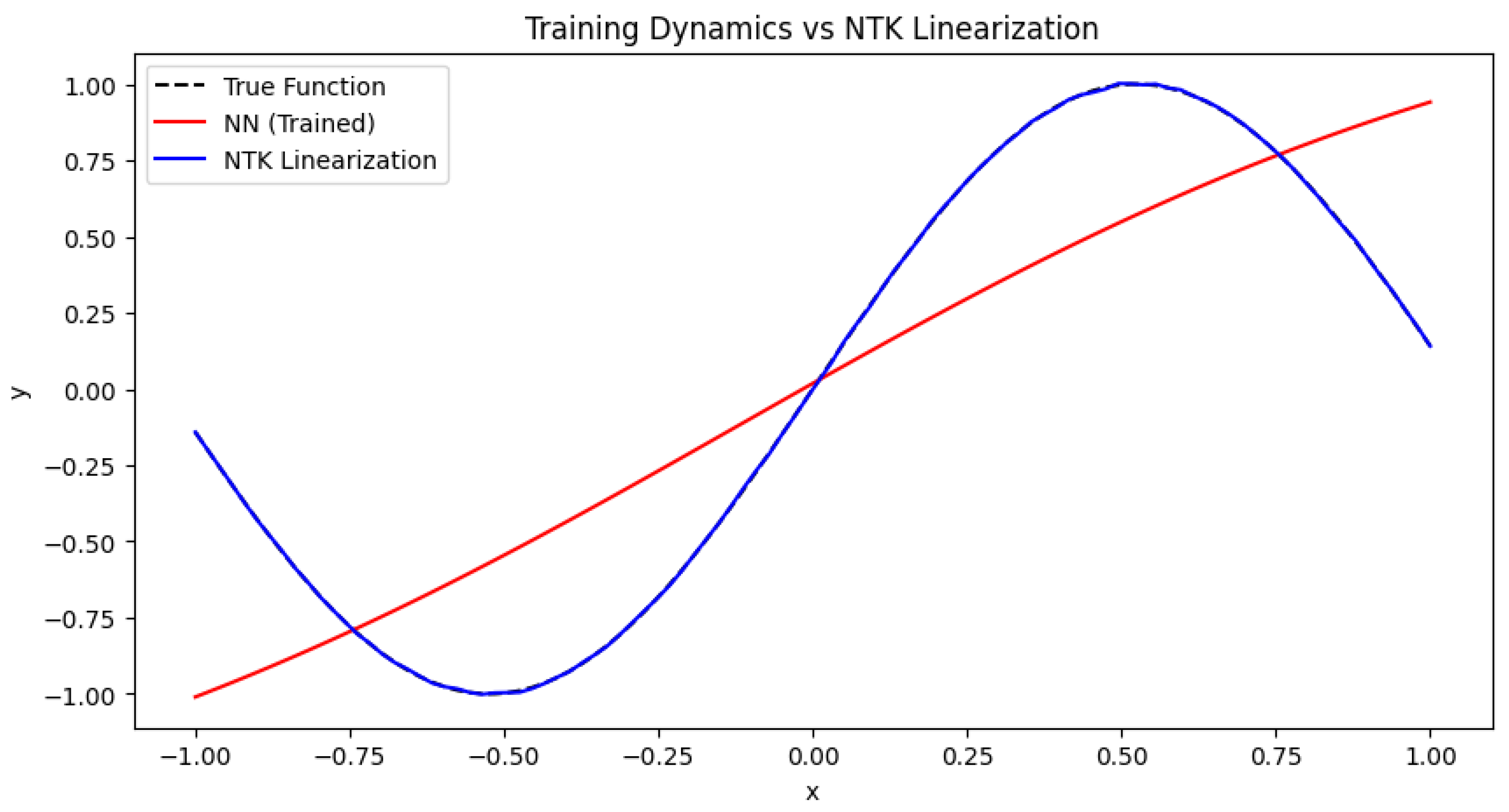
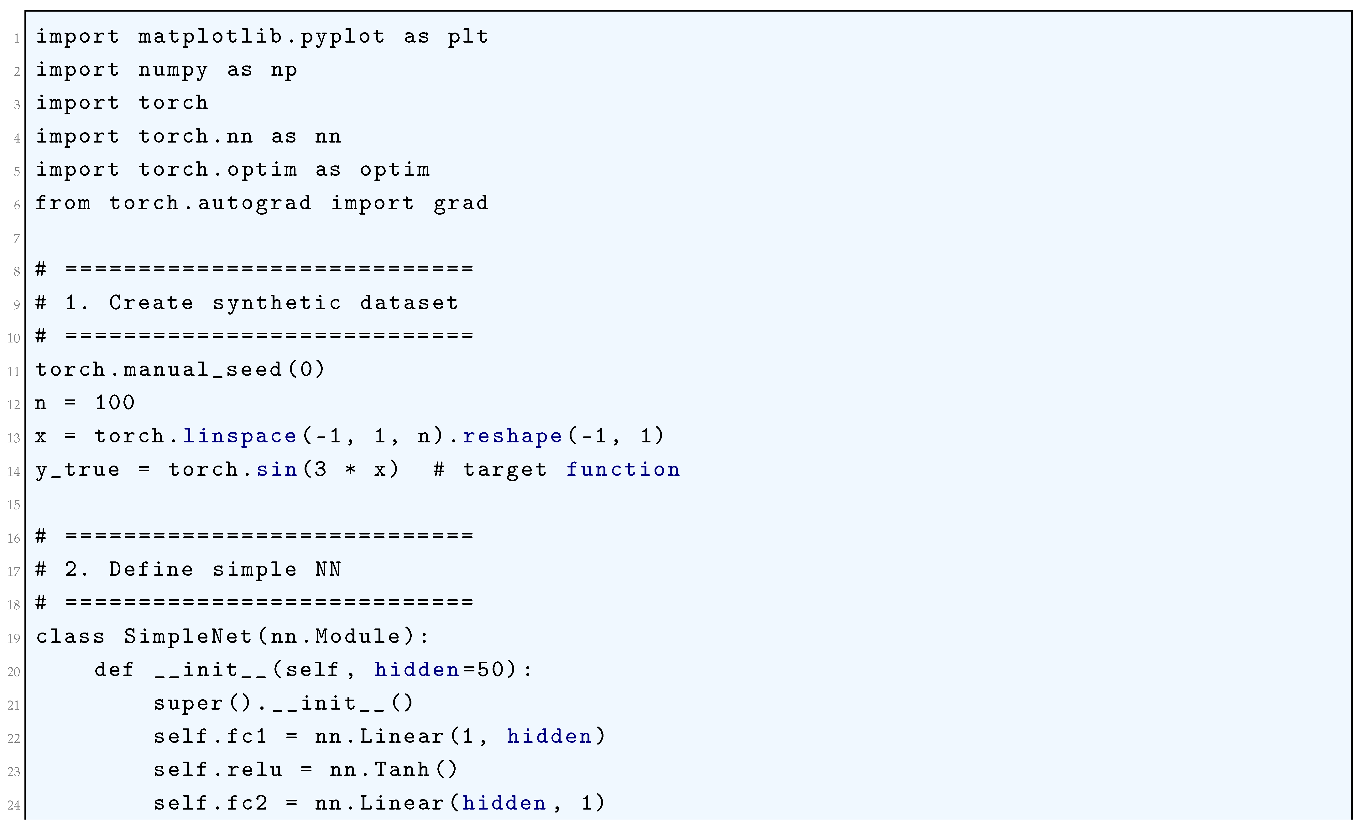
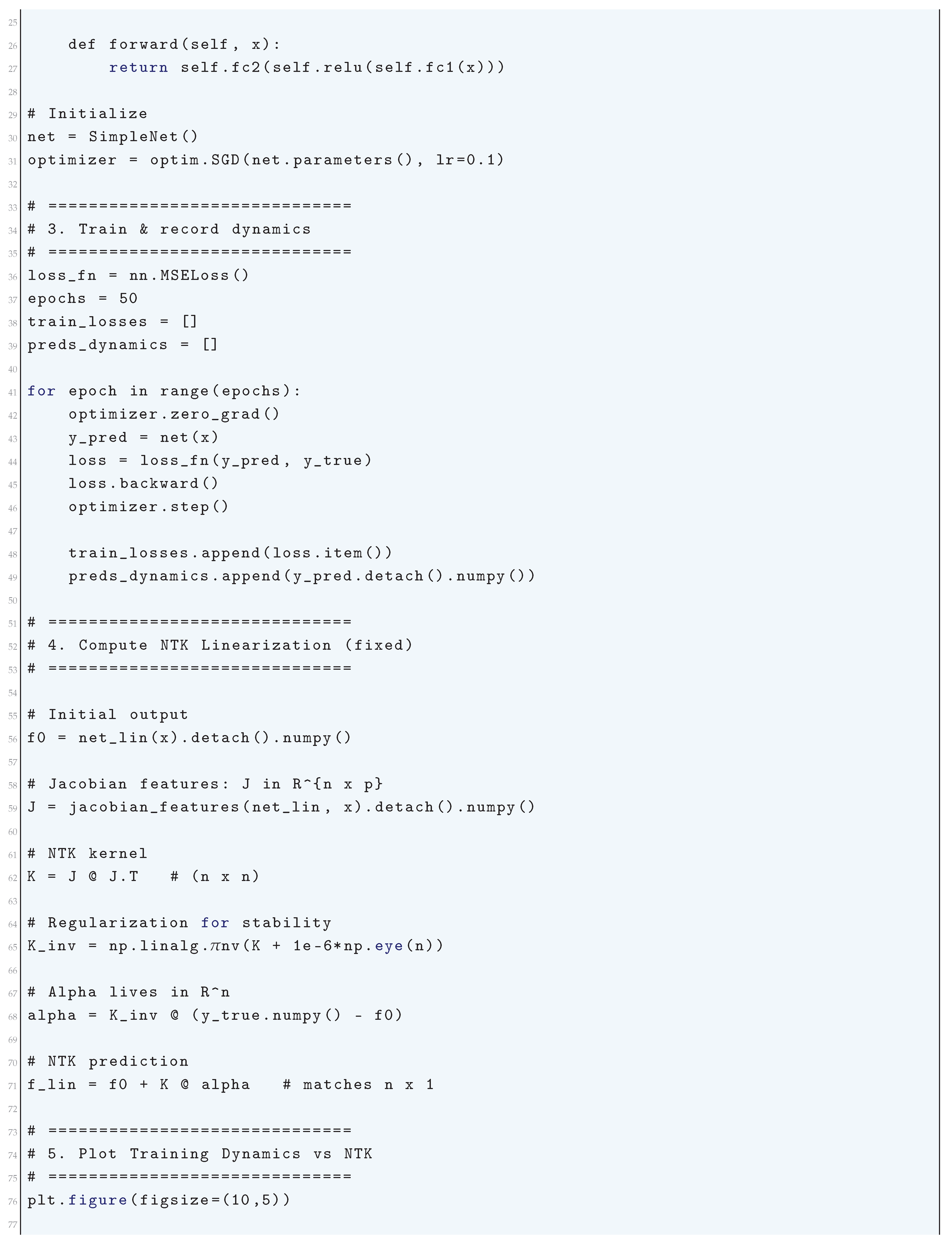
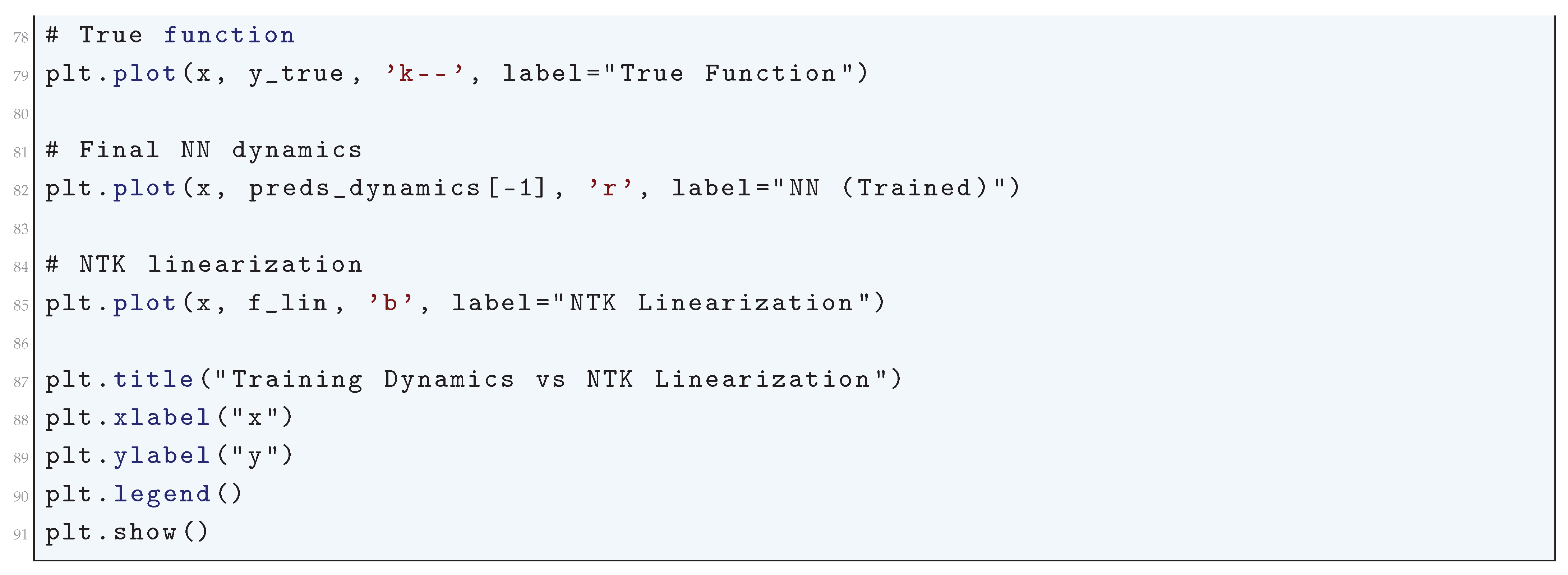
3.2. Literature Review of Training Dynamics and NTK Linearization
Trevisan et. al. [92] investigated how knowledge distillation can be analyzed using the Neural Tangent Kernel (NTK) framework and demonstrated that under certain conditions, the training dynamics of a student model in knowledge distillation closely follow NTK linearization. They explored how NTK affects generalization and feature transfer in the distillation process. They provided theoretical insight into why knowledge distillation improves performance in deep networks. Bonfanti et. al. (2024) [93] studied how NTK behaves in the nonlinear regime, particularly in Physics-Informed Neural Networks (PINNs). They showed that when PINNs operate outside the NTK regime, their performance degrades due to high sensitivity to initialization and weight updates. They established conditions under which NTK linearization is insufficient for PINNs, emphasizing the need for nonlinear adaptations. They provided practical guidelines for designing PINNs that maintain stable training dynamics. Jacot et. al. (2018) [94] introduced the Neural Tangent Kernel (NTK) as a fundamental framework for analyzing infinite-width neural networks. They proved that as width approaches infinity, neural networks evolve as linear models governed by the NTK. They derived generalization bounds for infinitely wide networks and connected training dynamics to kernel methods. They established NTK as a core tool in deep learning theory, leading to further developments in training dynamics research. Lee et. al. (2019) [95] extended NTK theory to arbitrarily deep networks, showing that even deep architectures behave as linear models under gradient descent and proved that training dynamics remain stable regardless of network depth when width is sufficiently large. They explored practical implications for initializing and optimizing deep networks. They strengthened NTK theory by confirming its validity beyond shallow networks. Yang and Hu (2022) [96] challenged the conventional NTK assumption that feature learning is negligible in infinite-width networks and showed that certain activation functions can induce nontrivial feature learning even in infinite-width regimes. They suggested that feature learning can be integrated into NTK theory, opening new directions in kernel-based deep learning research. Xiang et. al. (2023) [97] investigated how finite-width effects impact training dynamics under NTK assumptions and showed that finite-width networks deviate from NTK predictions due to higher-order corrections in weight updates. They derived corrections to NTK theory for practical networks, improving its predictive power for real-world architectures. They refined NTK approximations, making them more applicable to modern deep-learning models. Lee et. al. (2019) [98] extended NTK linearization to deep convolutional networks, analyzing their training dynamics under infinite width and showed how locality and weight sharing in CNNs impact NTK behavior. They also demonstrated practical consequences for CNN training in real-world applications. They bridged NTK theory and convolutional architectures, providing new theoretical tools for CNN analysis.
3.3. Gradient Flow and Stationary Points
3.3.1. Literature Review of Gradient Flow and Stationary Points
Goodfellow et. al. (2016) [120] provided a comprehensive overview of deep learning, including a detailed discussion of gradient-based optimization methods. It rigorously explains the dynamics of gradient descent in the context of neural networks, covering topics such as backpropagation, vanishing gradients, and saddle points. The book also discusses the role of learning rates, momentum, and adaptive optimization methods in shaping the trajectory of gradient flow. Sra et. al. (2012) [492] included several chapters dedicated to the theoretical and practical aspects of gradient-based optimization in machine learning. It provides rigorous mathematical treatments of gradient flow dynamics, including convergence analysis, the impact of stochasticity in stochastic gradient descent (SGD), and the geometry of loss landscapes in high-dimensional spaces. Choromanska et. al. (2015) [493] rigorously analyzed the loss surfaces of deep neural networks. It demonstrates that the loss landscape is highly non-convex but contains a large number of local minima that are close in function value to the global minimum. The paper provides insights into how gradient flow navigates these complex landscapes and why it often converges to satisfactory solutions despite the non-convexity. Arora et al. (2019) [494] provided a theoretical framework for understanding the dynamics of gradient descent in deep neural networks. It rigorously analyzes the role of overparameterization in enabling gradient flow to converge to global minima, even in the absence of explicit regularization. The paper also explores the implicit regularization effects of gradient descent and their impact on generalization. Du et. al. (2019) [485] establishes theoretical guarantees for the convergence of gradient descent to global minima in overparameterized neural networks. It rigorously proves that gradient flow can efficiently minimize the training loss to zero, even in the presence of non-convexity, by leveraging the high-dimensional geometry of the loss landscape. The authors provided a rigorous analysis of the exponential convergence of gradient descent in overparameterized neural networks. It shows that the gradient flow dynamics are characterized by a rapid decrease in the loss function, driven by the alignment of the network’s parameters with the data. The paper also discusses the role of initialization in shaping the trajectory of gradient flow. Zhang et al. (2017) [463] challenged traditional notions of generalization in deep learning. It rigorously demonstrates that deep neural networks can fit random labels, suggesting that the dynamics of gradient flow are not solely driven by the data distribution but also by the implicit biases of the optimization algorithm. The paper highlights the importance of understanding how gradient flow interacts with the architecture and initialization of neural networks. Baratin et. al. (2020) [495] explored the implicit regularization effects of gradient flow in deep learning from the perspective of function space. It rigorously demonstrates that gradient descent in overparameterized models tends to converge to solutions that minimize certain norms or complexity measures, providing insights into why these models generalize well despite their capacity to overfit. Balduzzi et al. (2018) [496] extended the analysis of gradient flow to multi-agent optimization problems, such as those encountered in generative adversarial networks (GANs). It rigorously characterizes the dynamics of gradient descent in games, highlighting the role of rotational forces and the challenges of convergence in non-cooperative settings. The paper provides tools for understanding how gradient flow behaves in complex, interactive learning scenarios. Allen-Zhu et al. (2019) [487] provided a rigorous convergence theory for deep learning models trained with gradient descent. It shows that overparameterization enables gradient flow to avoid bad local minima and converge to global minima efficiently. The paper also analyzes the role of initialization, step size, and network depth in shaping the dynamics of gradient descent.
3.3.2. Analysis of Gradient Flow and Stationary Points
The dynamics of gradient flow in neural network training are fundamentally governed by the continuous evolution of parameters under the influence of the negative gradient of the loss function, expressed as
The loss function, typically of the form
measures the discrepancy between the network’s predicted outputs and the true labels . At stationary points of the flow, the condition
holds, indicating that the gradient vanishes. To classify these stationary points, the Hessian matrix is examined. For eigenvalues of H, the nature of the stationary point is determined: for all i corresponds to a local minimum, for all i to a local maximum, and mixed signs indicate a saddle point.Under gradient flow , the trajectory converges to critical points:
The gradient flow also governs the temporal evolution of the network’s predictions . A Taylor series expansion of about an initial parameter gives:
where is the Jacobian and is the Hessian of with respect to .
In the NTK (neural tangent kernel) regime, higher-order terms are negligible due to the large parameterization of the network, and the linear approximation suffices:
Under gradient flow, the time derivative of the network’s predictions is given by:
Substituting the parameter dynamics , this becomes:
Defining the NTK as , and assuming constancy of the NTK during training (), the evolution equation simplifies to:
Rewriting in matrix form, let and . The NTK matrix evaluated at initialization defines the system:
The solution to this linear system is:
As , the predictions converge to the labels: , implying zero training error. The eigenvalues of determine the rates of convergence. Diagonalizing as , where Q is orthogonal and , the dynamics in the eigenbasis are:
with and . Solving, we obtain:
Each mode decays exponentially with a rate proportional to the eigenvalue . Modes with larger converge faster, while smaller eigenvalues slow convergence.
The NTK framework thus rigorously explains the linearization of training dynamics in overparameterized neural networks. This linear behavior ensures that the optimization trajectory remains within a convex region of the parameter space, leading to both convergence and generalization. By leveraging the constancy of the NTK, the complexity of nonlinear neural networks is reduced to an analytically tractable framework that aligns closely with empirical observations.
3.3.3. Hessian Structure
The Hessian matrix, , serves as a critical construct in the mathematical framework of optimization, capturing the second-order partial derivatives of the loss function with respect to the parameter vector . Each element reflects the curvature of the loss surface along the -direction. The symmetry of , guaranteed by the Schwarz theorem under the assumption of continuous second partial derivatives, implies . This property ensures that the eigenvalues of are real and the eigenvectors are orthogonal, satisfying the eigenvalue equation
The behavior of the loss function around a specific parameter value can be rigorously analyzed using a second-order Taylor expansion. This expansion is given by:
Here, the term represents the linear variation of the loss, while the quadratic term describes the curvature effects. The eigenvalues of dictate the nature of the critical point . Specifically, if all , is a local minimum; if all , it is a local maximum; and if the eigenvalues have mixed signs, is a saddle point. The leading-order approximation to the change in the loss function, , highlights the dependence on the eigenstructure of . In the context of gradient descent, parameter updates follow the iterative scheme:
where is the learning rate. Substituting the Taylor expansion of around gives:
To analyze this update rigorously, we project onto the eigenbasis of , expressing it as:
where . Substituting this expansion into the gradient descent update rule yields:
The convergence of this iterative scheme is governed by the condition , which constrains the learning rate relative to the spectrum of . For eigenvalues with large magnitudes, excessively large learning rates can cause oscillatory or divergent updates.
In the Neural Tangent Kernel (NTK) regime, the evolution of a neural network during training can be approximated by a linearization of the network output around the initialization. Let denote the output of the network for input x. Linearizing around gives:
The NTK, defined as:
remains approximately constant during training for sufficiently wide networks. The training dynamics of the parameters are described by:
which, under the NTK approximation, becomes:
where K is the NTK matrix evaluated at initialization. The evolution of the loss function is governed by the eigenvalues of K, which control the rate of convergence in different directions.
The spectral properties of the Hessian play a pivotal role in the generalization properties of neural networks. Empirical studies reveal that the eigenvalue spectrum of often exhibits a "bulk-and-spike" structure, with a dense bulk of eigenvalues near zero and a few large outliers. The bulk corresponds to flat directions in the loss landscape, which contribute to the robustness and generalization of the model, while the spikes represent sharp directions associated with overfitting. This spectral structure can be analyzed using random matrix theory, where the density of eigenvalues is modeled by distributions such as the Marchenko-Pastur law:
where are the spectral bounds and is the ratio of the number of parameters to the number of data points. This rigorous analysis links the Hessian structure to both the optimization dynamics and the generalization performance of neural networks, providing a comprehensive mathematical understanding of the training process. The Hessian satisfies:
For overparameterized networks, is nearly degenerate, implying the existence of flat minima.
3.3.4. NTK Linearization
The dynamics of neural networks under gradient flow can be comprehensively described by beginning with the parameterized representation of the network , where denotes the set of trainable parameters, is the input, and represents the output. The objective of training is to minimize a loss function , defined over a dataset , where and represent the input-target pairs. The evolution of the parameters during training is governed by the gradient flow equation , where is the gradient of the loss function with respect to the parameters. To analyze the dynamics of the network outputs, we first consider the time derivative of . Using the chain rule, this is expressed as:
Substituting , we have:
The gradient of the loss function, , can be expressed explicitly in terms of the training data. For a generic loss function over the dataset, this takes the form:
where represents the loss for the i-th data point. The gradient of the loss with respect to the parameters is therefore given by:
Substituting this back into the time derivative of , we obtain:
To introduce the Neural Tangent Kernel (NTK), we define it as the Gram matrix of the Jacobians of the network output with respect to the parameters:
Using this definition, the time evolution of the output becomes:
In the overparameterized regime, where the number of parameters p is significantly larger than the number of training data points n, it has been empirically and theoretically observed that the NTK remains nearly constant during training.
Specifically, , where represents the parameters at initialization. This constancy significantly simplifies the analysis of the network’s training dynamics. To see this, consider the solution to the differential equation governing the output dynamics. Let represent the matrix of network outputs for all training inputs, where the i-th row corresponds to . The dynamics can be expressed in matrix form as:
where is the NTK matrix evaluated at initialization, and is the gradient of the loss with respect to the output matrix F. For the special case of a mean squared error loss, , where is the matrix of target outputs, the gradient simplifies to:
Substituting this into the dynamics, we obtain:
The solution to this differential equation is:
where represents the initial outputs of the network. As , the exponential term vanishes, and the network outputs converge to the targets Y, provided that is positive definite. The rate of convergence is determined by the eigenvalues of , with smaller eigenvalues corresponding to slower convergence along the associated eigenvectors. To understand the stationary points of this system, we note that these occur when . From the dynamics, this implies:
If is invertible, this yields , indicating that the network exactly interpolates the training data at the stationary point. However, if is not full-rank, the stationary points form a subspace of solutions satisfying , where is the projection operator onto the column space of .
The NTK framework provides a mathematically rigorous lens to analyze training dynamics, elucidating the interplay between parameter evolution, kernel properties, and loss convergence in neural networks. By linearizing the training dynamics through the NTK, we achieve a deep understanding of how overparameterized networks evolve under gradient flow and how they reach stationary points, revealing their capacity to interpolate data with remarkable precision.
3.3.5. Python Code to Generate Figure 31 Illustrating the Gradient Flow and Stationary Points
The Python code below produces the Figure 31 illustrating the Gradient Flow and Stationary Points.
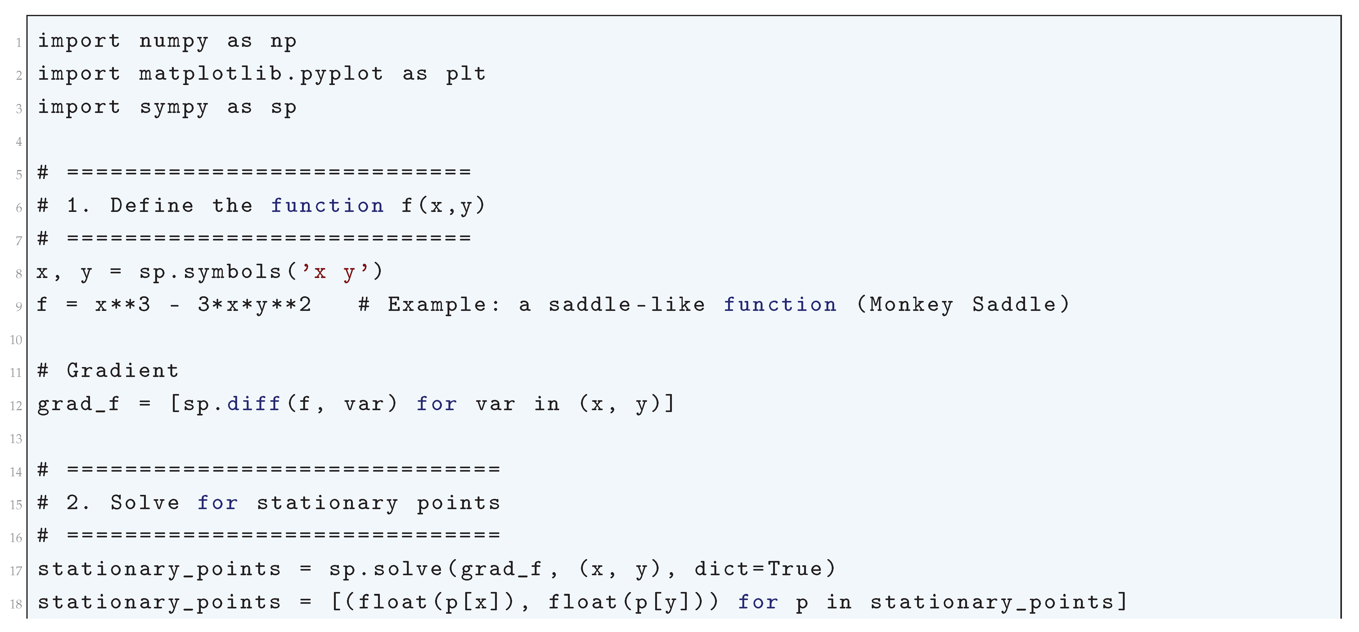
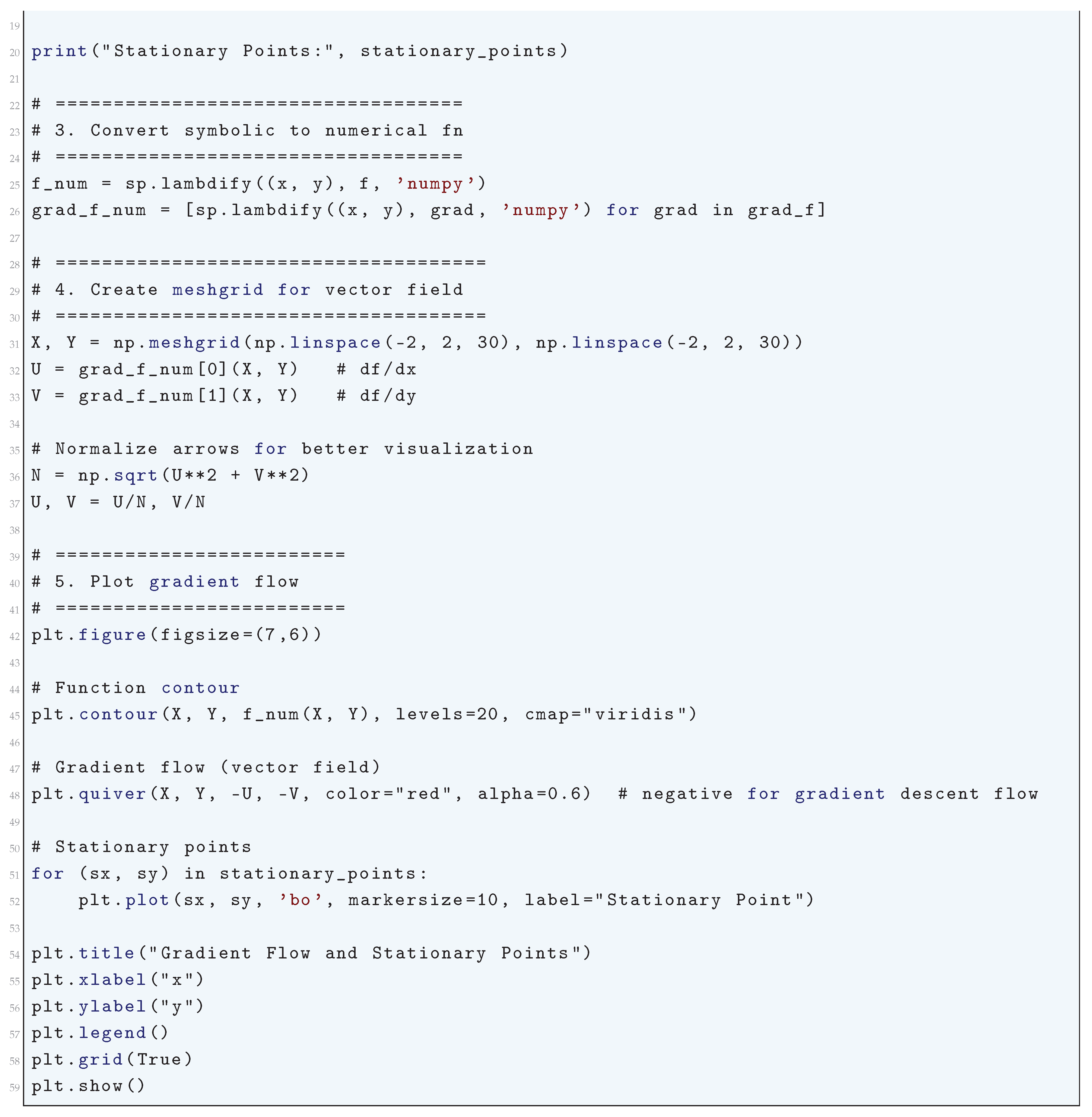
Figure 31.
Gradient Flow and Stationary Points
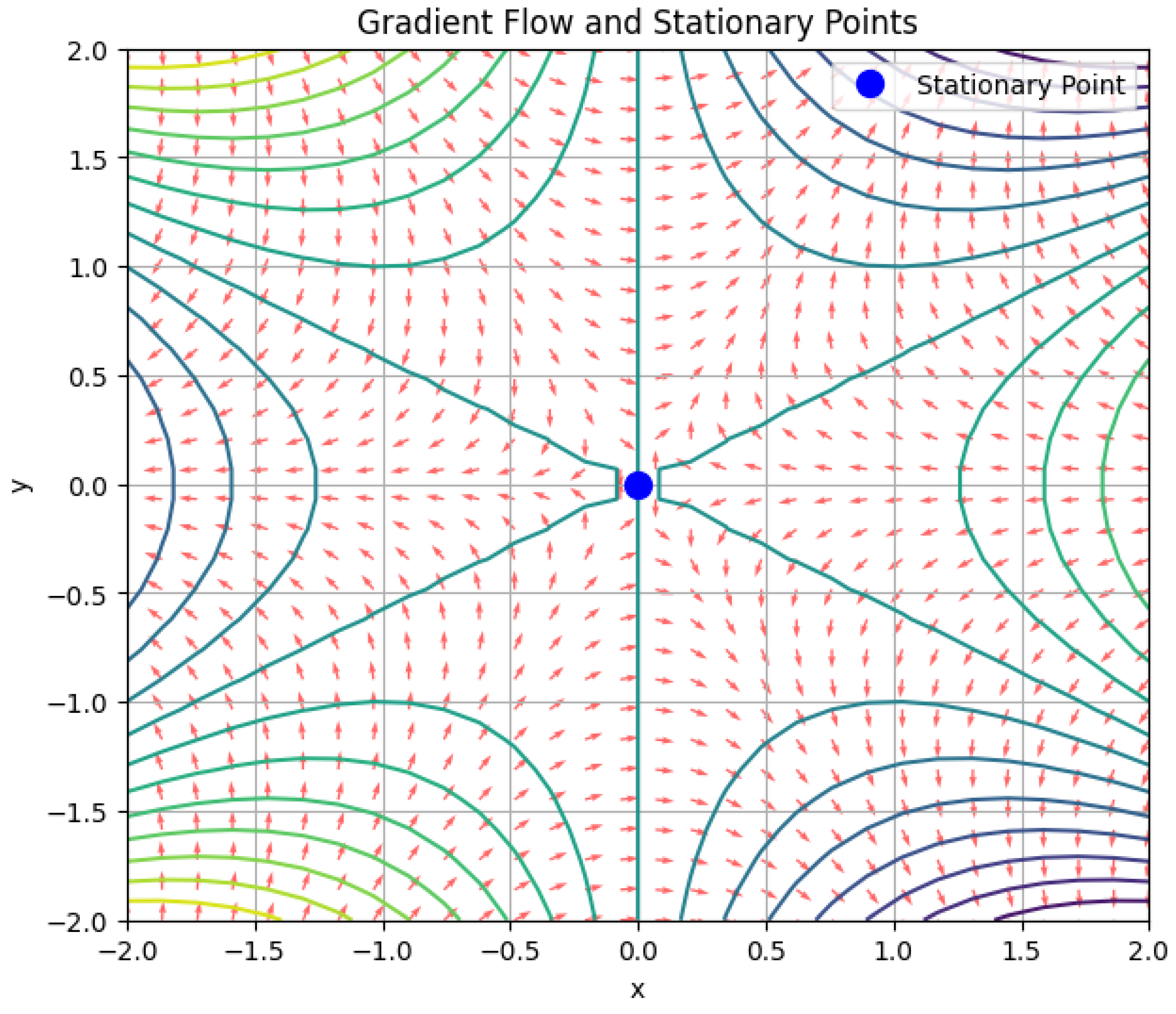
3.3.6. Python Code to Generate Figure 32 and Figure 33 Illustrating the Hessian Structure
Figure 32.
Hessian Structure (NTK Regime) & NTK Matrix
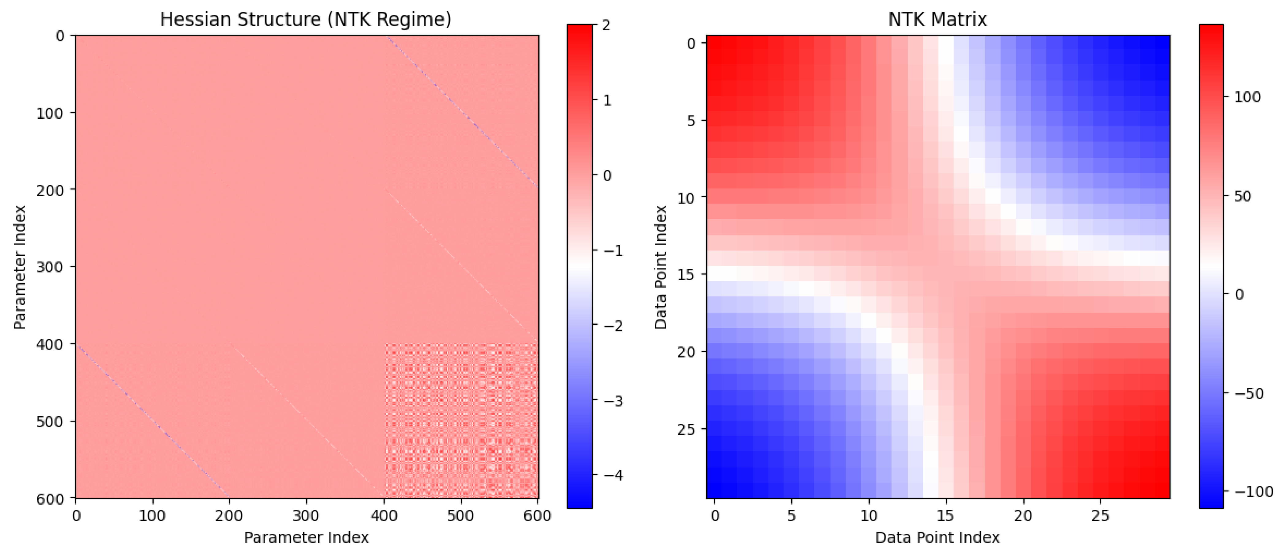
Figure 33.
Hessian Spectrum (NTK Regime)
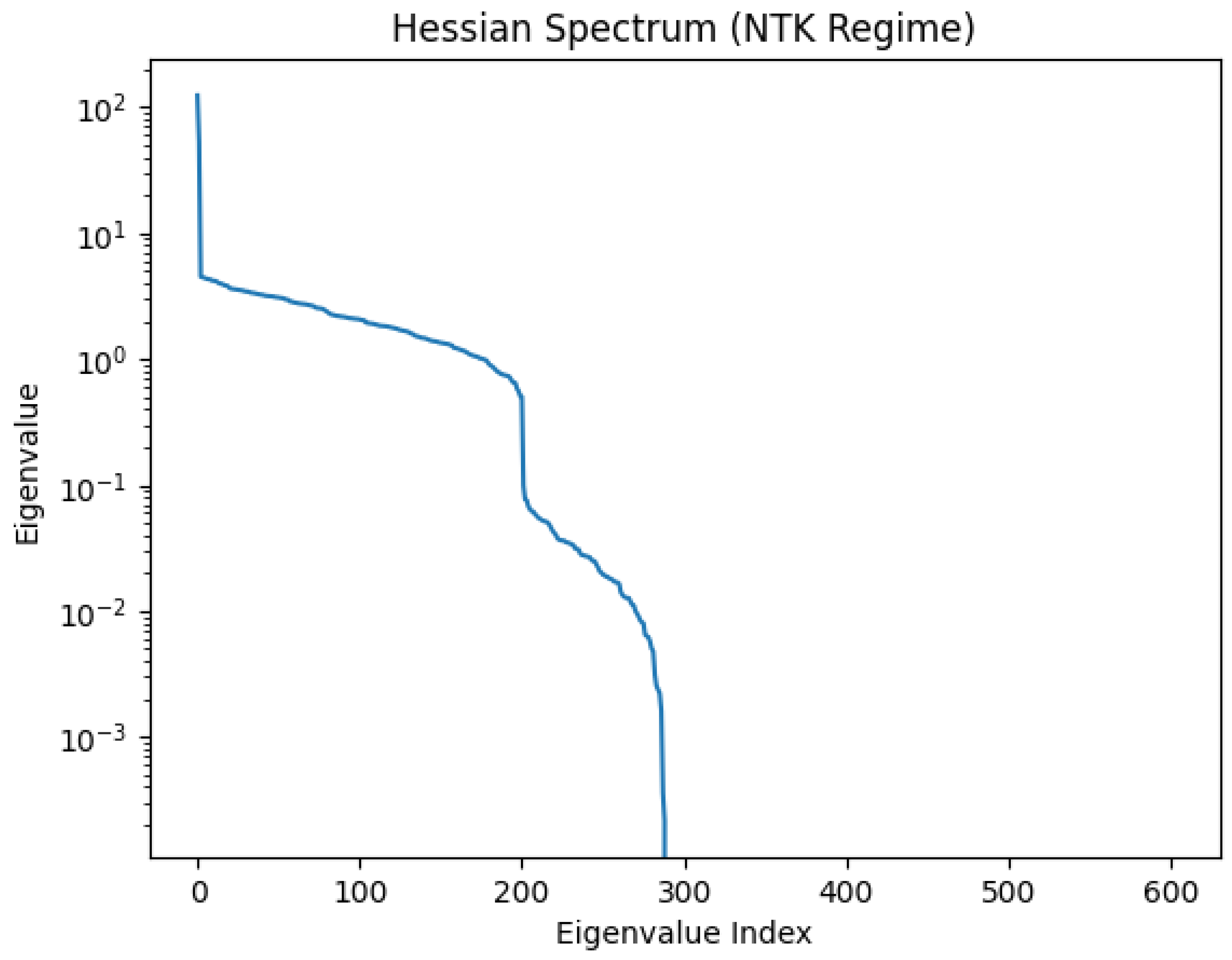
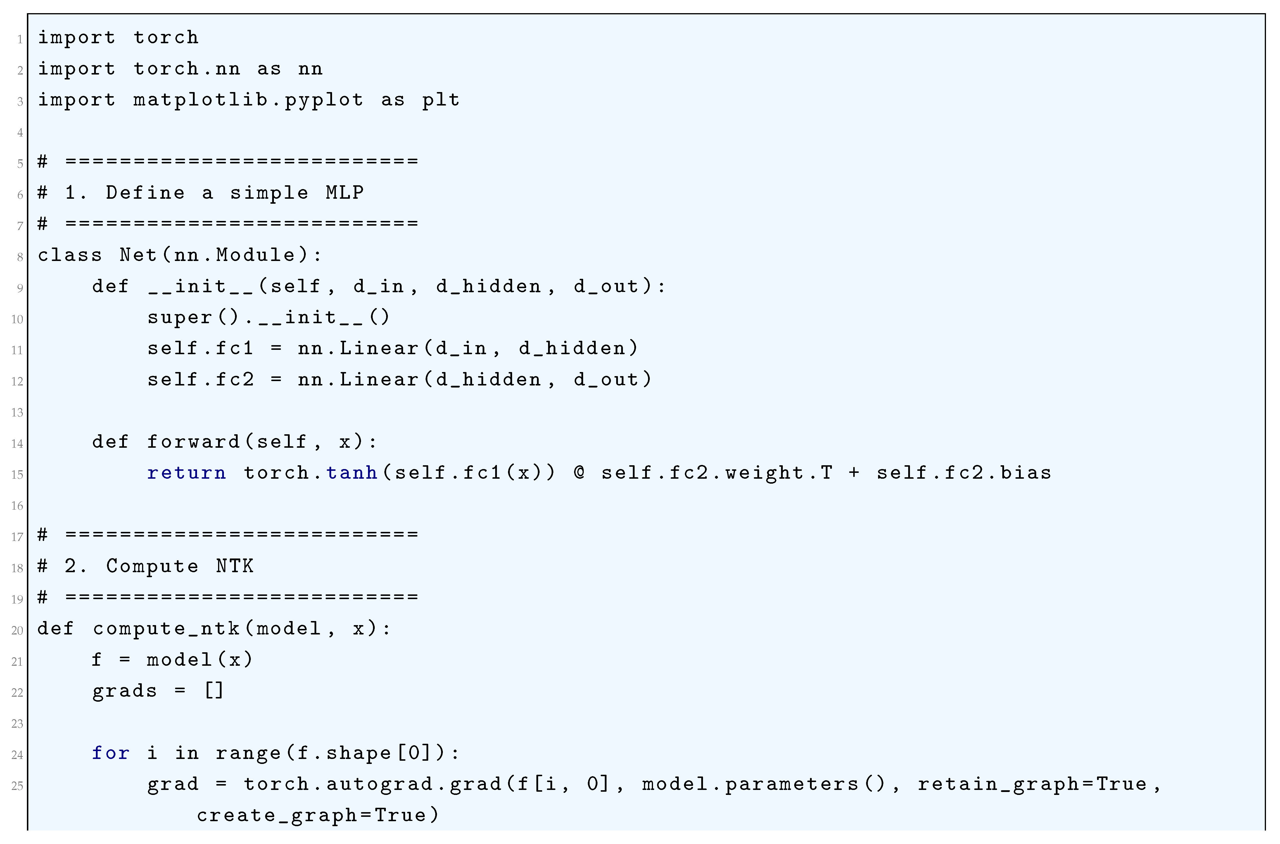
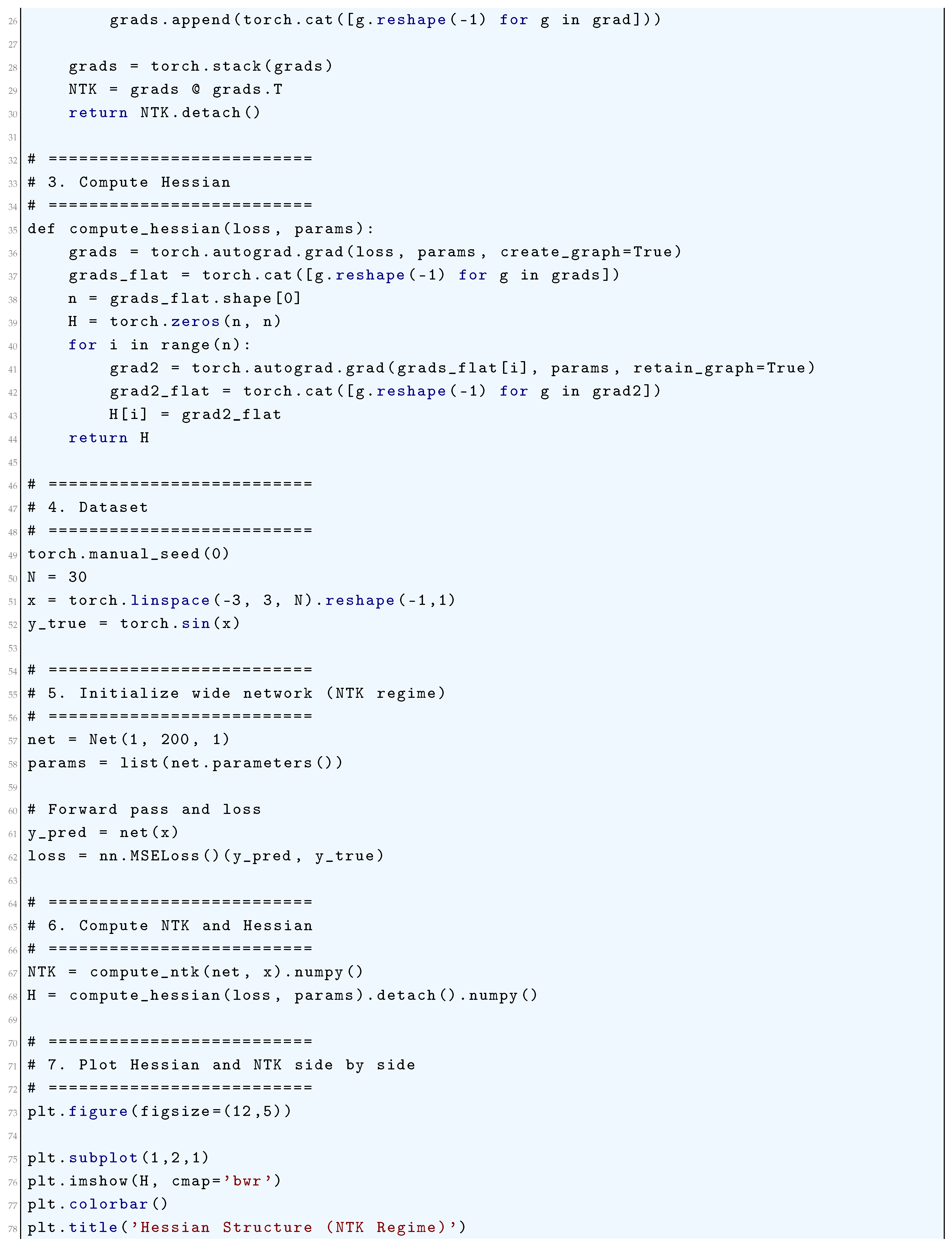
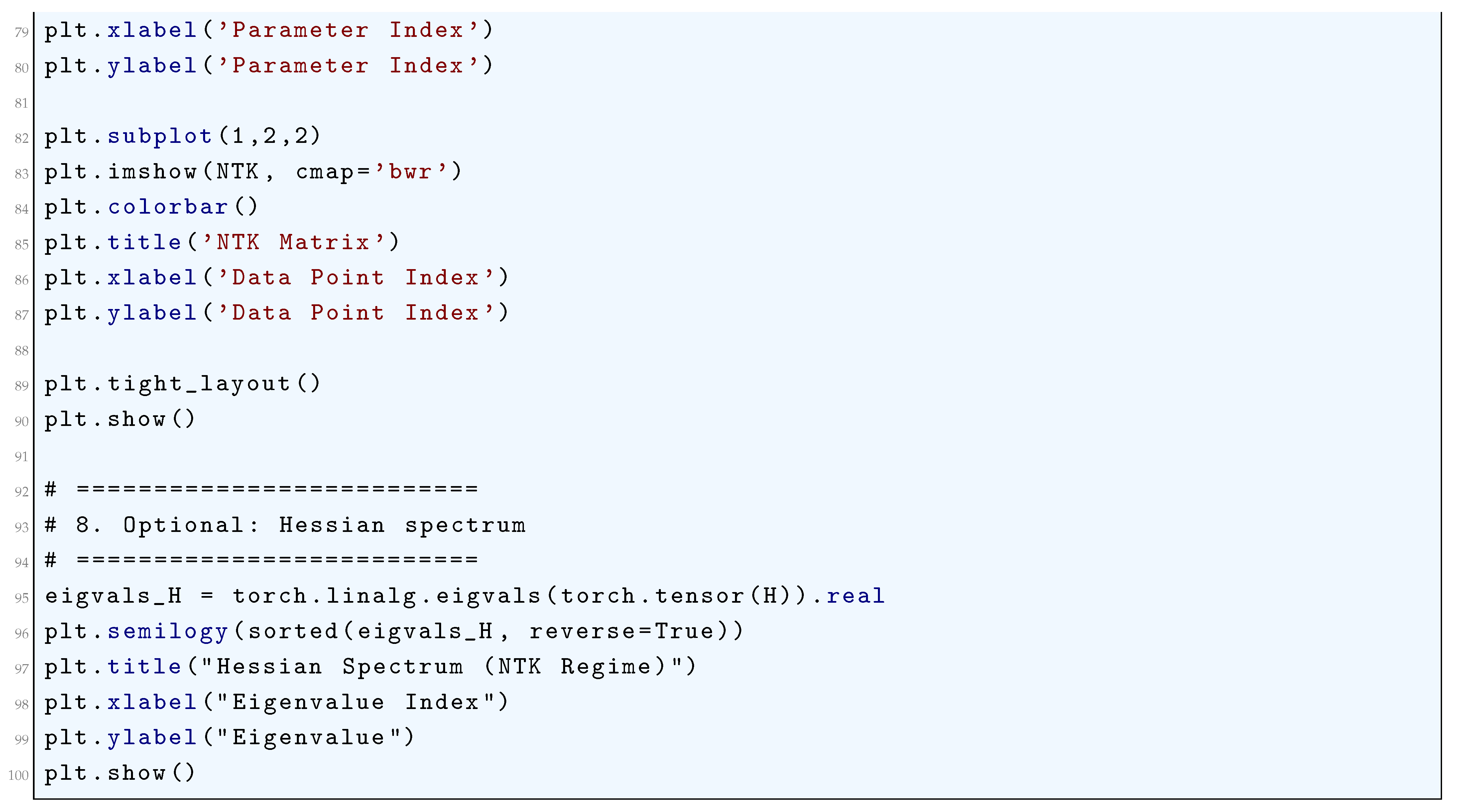
3.3.7. Python Code to Generate Figure 34 Illustrating the Final Fit & Training Dynamics (NN vs NTK)
The Python code below produces the Figure 34 illustrating the Final Fit & Training Dynamics (NN vs NTK).
Figure 34.
Final Fit & Training Dynamics (NN vs NTK)
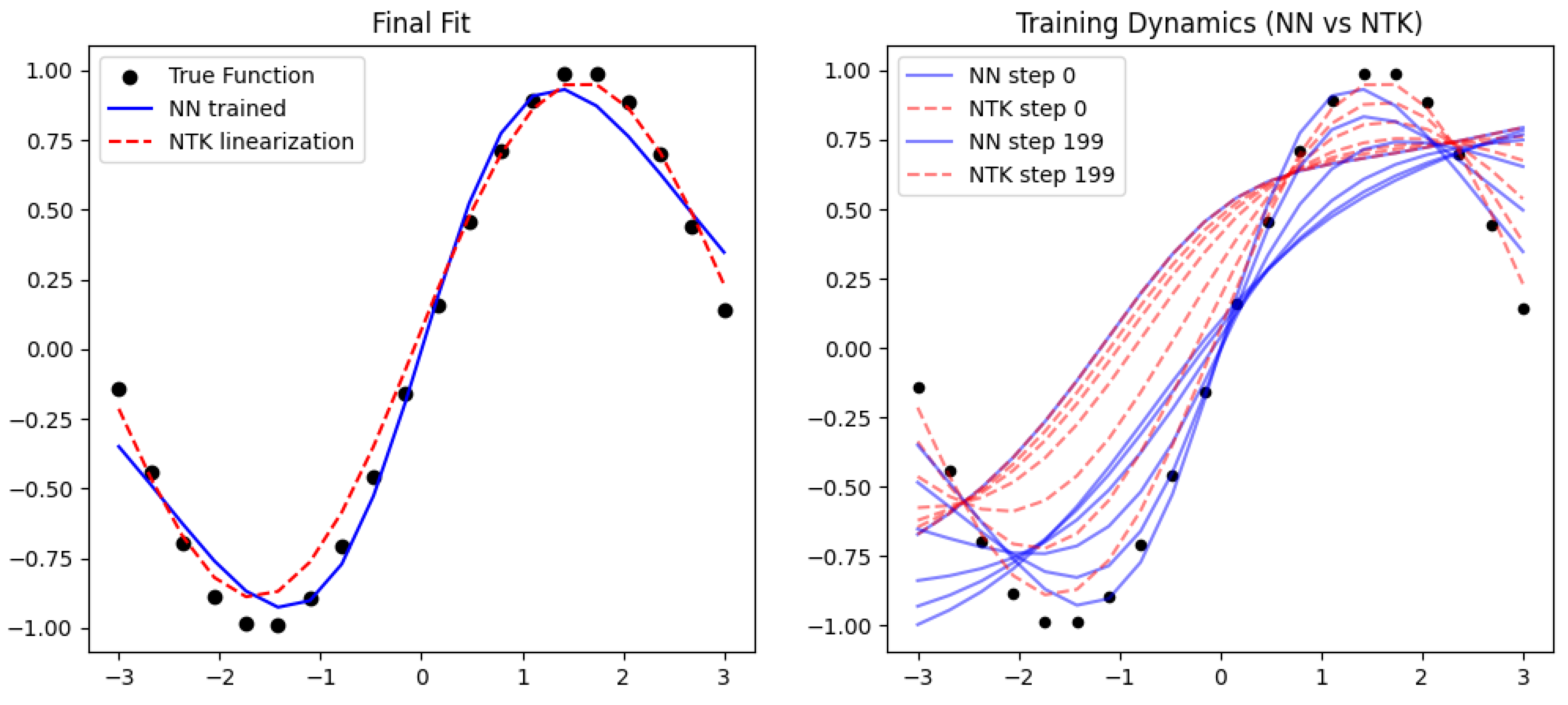
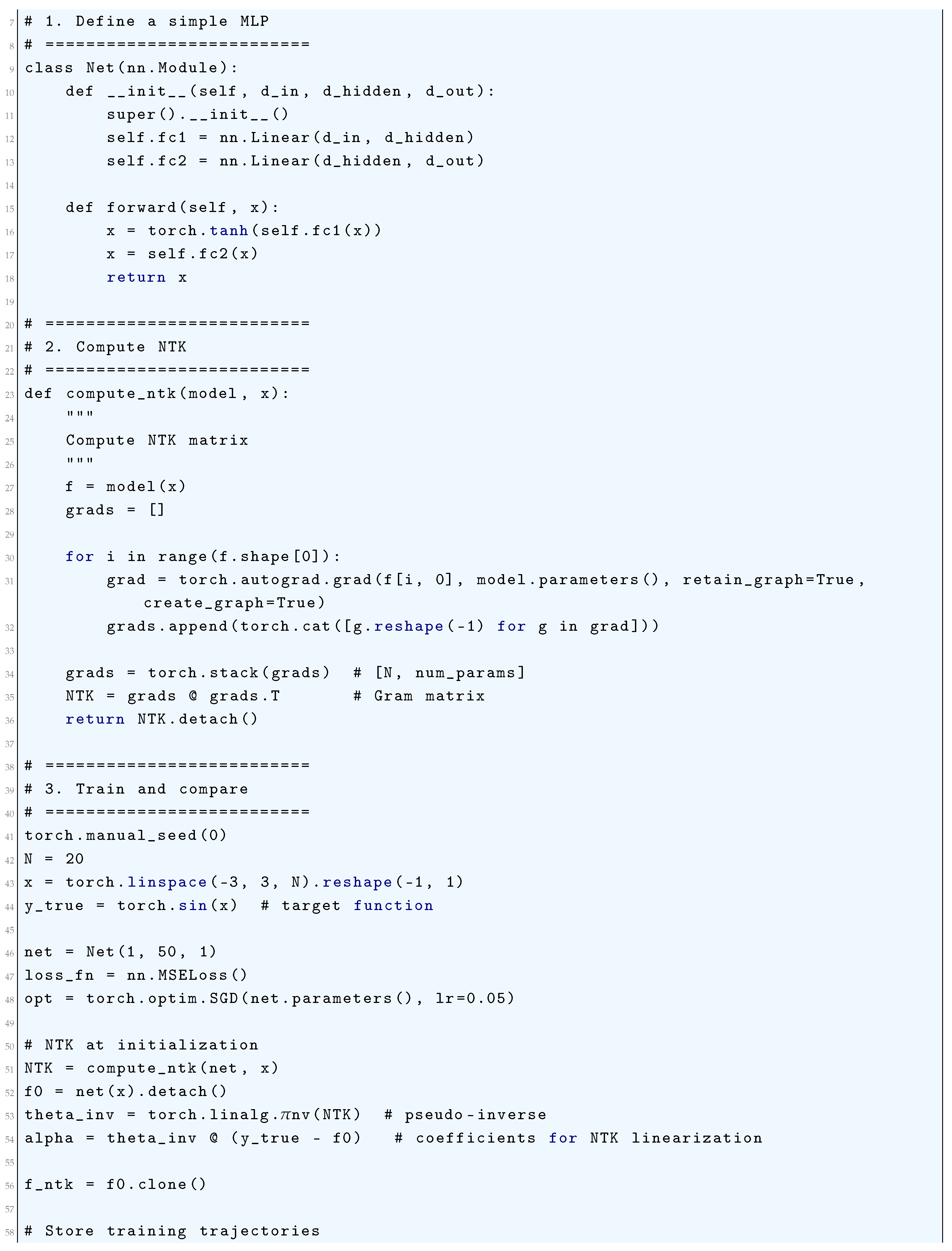
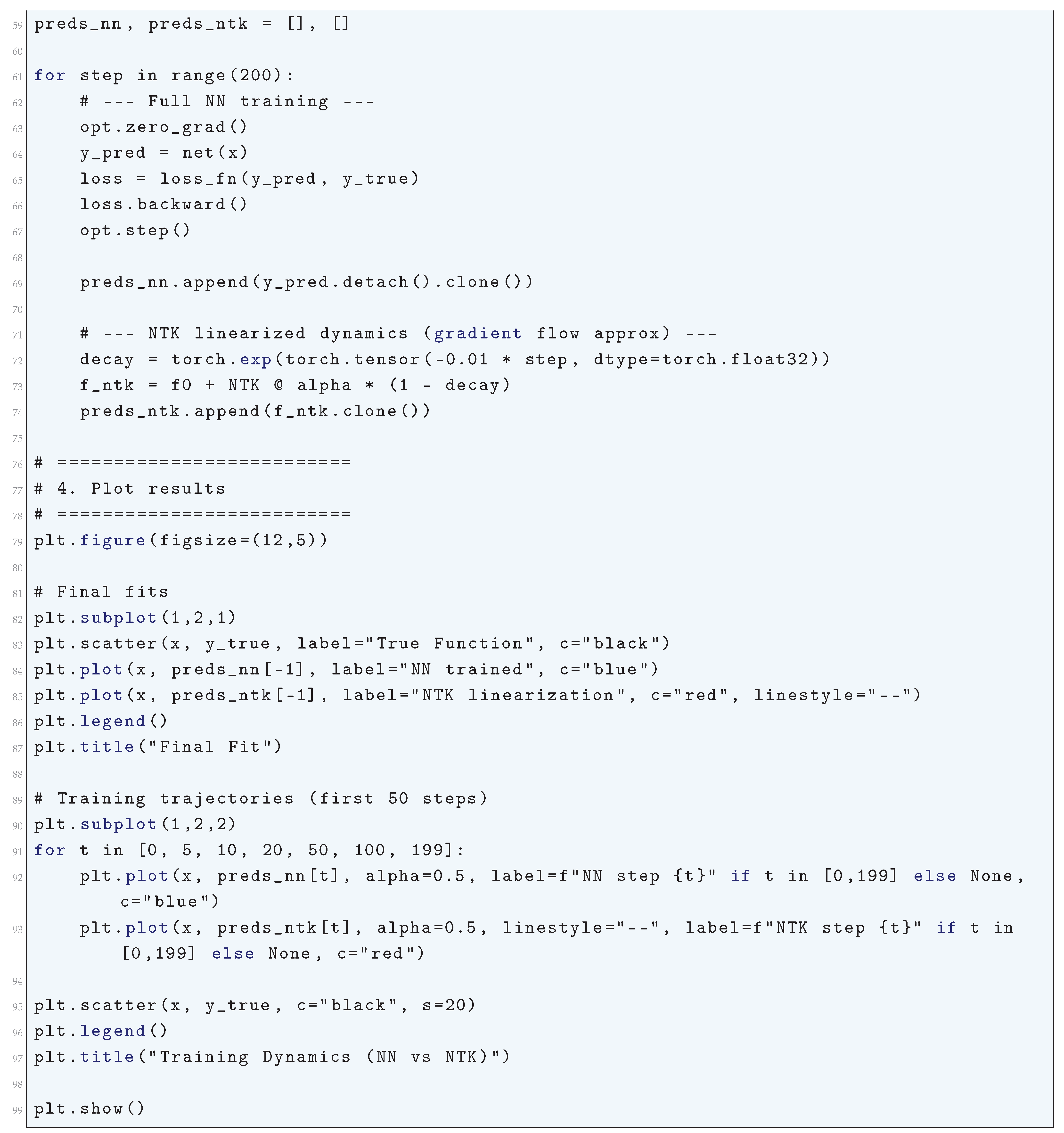
3.4. NTK Regime
3.4.1. Literature Review of NTK Regime
Jacot et. al. (2018) [94] in a seminal paper introduced the Neural Tangent Kernel (NTK) and establishes its theoretical foundation. The authors show that in the infinite-width limit, the dynamics of gradient descent in neural networks can be described by a kernel method, where the NTK remains constant during training. This work bridges the gap between deep learning and kernel methods, providing a framework to analyze the training and generalization of wide neural networks. Lee et. al. (2017) [95] did a work that predates the NTK but lays the groundwork by showing that infinitely wide neural networks behave as Gaussian processes. The authors derive the kernel corresponding to such networks, which is a precursor to the NTK. This paper is crucial for understanding the connection between neural networks and kernel methods. Chizat and Bach (2018) [484] provided a rigorous analysis of gradient descent in over-parameterized models, including neural networks. It complements the NTK framework by showing that gradient descent converges to global minima in such settings. The work highlights the role of over-parameterization in simplifying the optimization landscape. Du et. al. (2019) [485] proved that gradient descent can find global minima in deep neural networks under the NTK regime. The authors provide explicit convergence rates and show that the NTK framework guarantees efficient optimization for wide networks. This work strengthens the theoretical understanding of why deep learning works. Arora et. al. (2019) [486] provided a fine-grained analysis of optimization and generalization in two-layer neural networks under the NTK regime. It establishes precise bounds on the generalization error and shows how over-parameterization leads to benign optimization landscapes. Allen-Zhu et. al. (2019) [487] extended the NTK framework to deep networks and provided a comprehensive convergence theory for over-parameterized neural networks. The authors show that gradient descent converges to global minima and that the NTK remains approximately constant during training. Cao and Gu (2019) [488] derived generalization bounds for wide and deep neural networks trained with stochastic gradient descent (SGD) under the NTK regime. It highlights the role of the NTK in controlling the generalization error and provides insights into the implicit regularization of SGD. Yang (2019) [489] generalized the NTK framework to architectures with weight sharing, such as convolutional neural networks (CNNs). The author derives the NTK for such architectures and shows that they also exhibit Gaussian process behavior in the infinite-width limit. Huang and Yau (2020) [490] extended the NTK framework by introducing the Neural Tangent Hierarchy (NTH), which captures higher-order interactions in the training dynamics of deep networks. The authors provide a more refined analysis of the training process beyond the first-order approximation of the NTK. Belkin et. al. (2019) [491] explored the connection between deep learning and kernel learning, emphasizing the role of the NTK in understanding generalization and optimization. It provides a high-level perspective on why the NTK framework is essential for analyzing modern machine learning models.
3.4.2. Analysis of NTK Regime
The Neural Tangent Kernel (NTK) regime is a fundamental framework for understanding the dynamics of gradient descent in highly overparameterized neural networks. Consider a neural network parameterized by , where P represents the total number of parameters, and is the input vector. For a training dataset , the loss function at time t is given by
The parameters evolve according to gradient descent as , where is the learning rate.
In the NTK regime, we consider the first-order Taylor expansion of the network output around the initialization :
This linear approximation transforms the nonlinear dynamics of f into a simpler, linearized form. To analyze training, we introduce the Jacobian matrix , where . The vector of outputs , aggregating predictions over the dataset, evolves as
The NTK is defined as
As , the NTK converges to a deterministic matrix that remains nearly constant during training. Substituting the linearized form of into the gradient descent update equation gives
where is the vector of true labels. Defining the residual , the dynamics of training reduce to
The eigendecomposition , with orthogonal Q and diagonal , allows us to analyze the decay of residuals in the eigenbasis of :
where . Each component decays as
For small , the training dynamics are approximately continuous, governed by
leading to the solution
The NTK for specific architectures, such as fully connected ReLU networks, can be derived using layerwise covariance matrices. Let denote the covariance between pre-activations at layer l. The recurrence relation for is
where The NTK, a sum over contributions from all layers, quantifies how parameter updates propagate through the network.
In the infinite-width limit, the NTK framework predicts generalization properties, as the kernel matrix governs both training and test-time behavior. The NTK connects neural networks to classical kernel methods, offering a bridge between deep learning and well-established theoretical tools in approximation theory. This regime’s deterministic and analytical tractability enables precise characterizations of network performance, convergence rates, and robustness to initialization and learning rate variations.
3.4.3. Python Code to Generate Figure 35 Illustrating the Final Predictions in NTK Regime & Training Dynamics (NN vs NTK)
The Python code below produces the Figure 35 Illustrating the Final Predictions in NTK Regime & Training Dynamics (NN vs NTK).
Figure 35.
Final Predictions in NTK Regime & Training Dynamics (NN vs NTK)
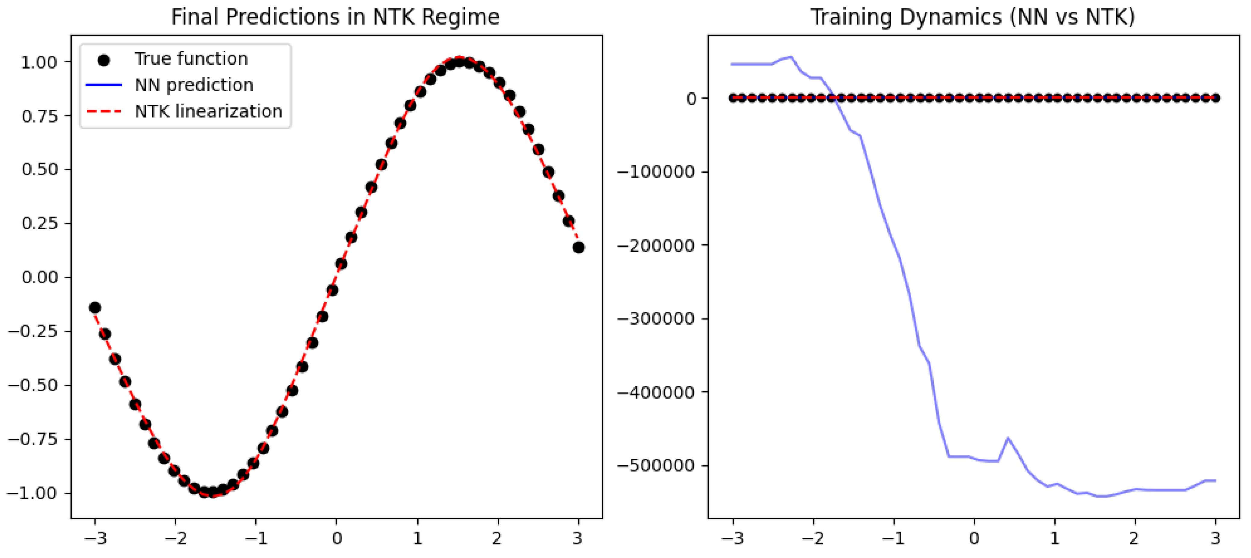
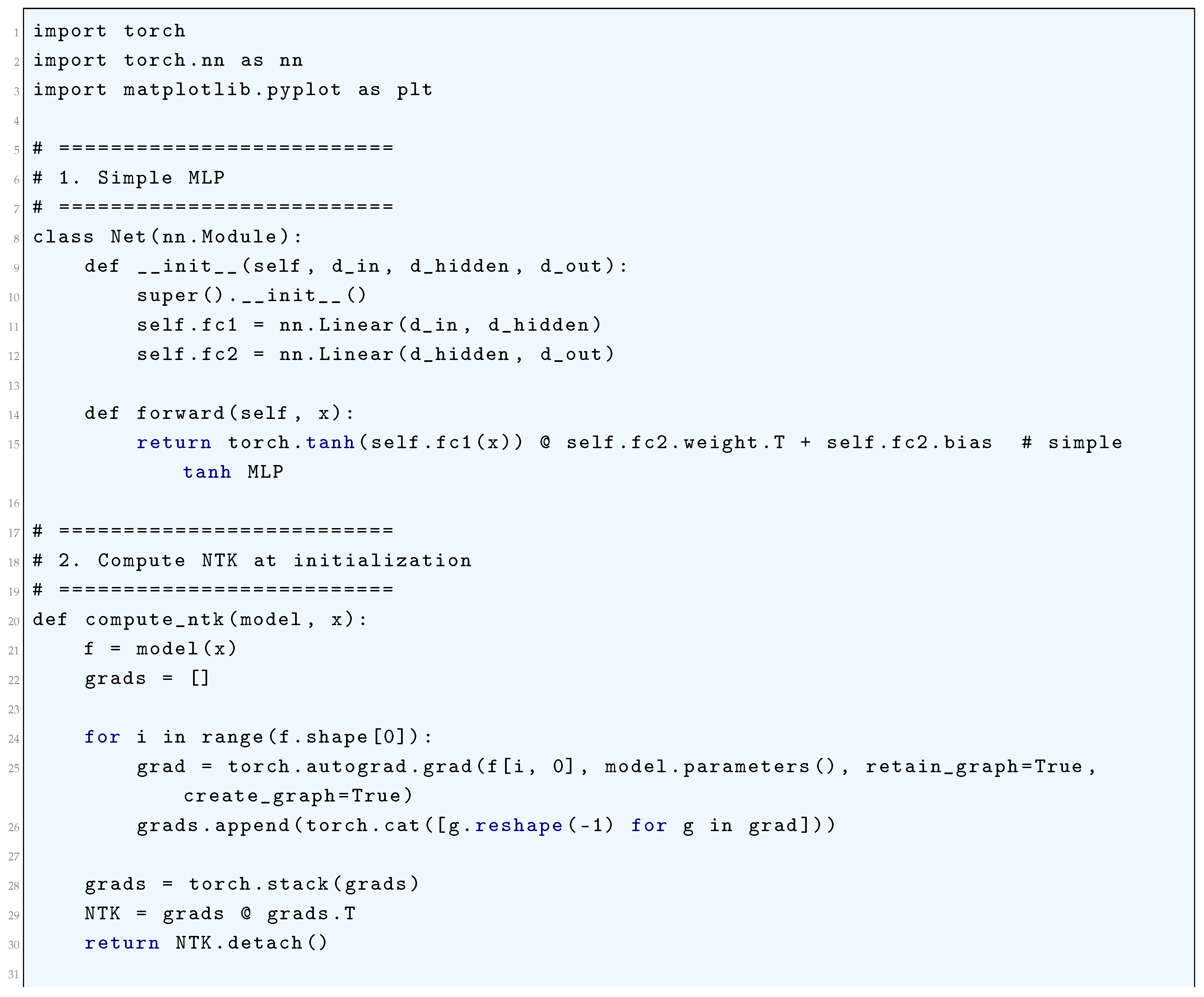
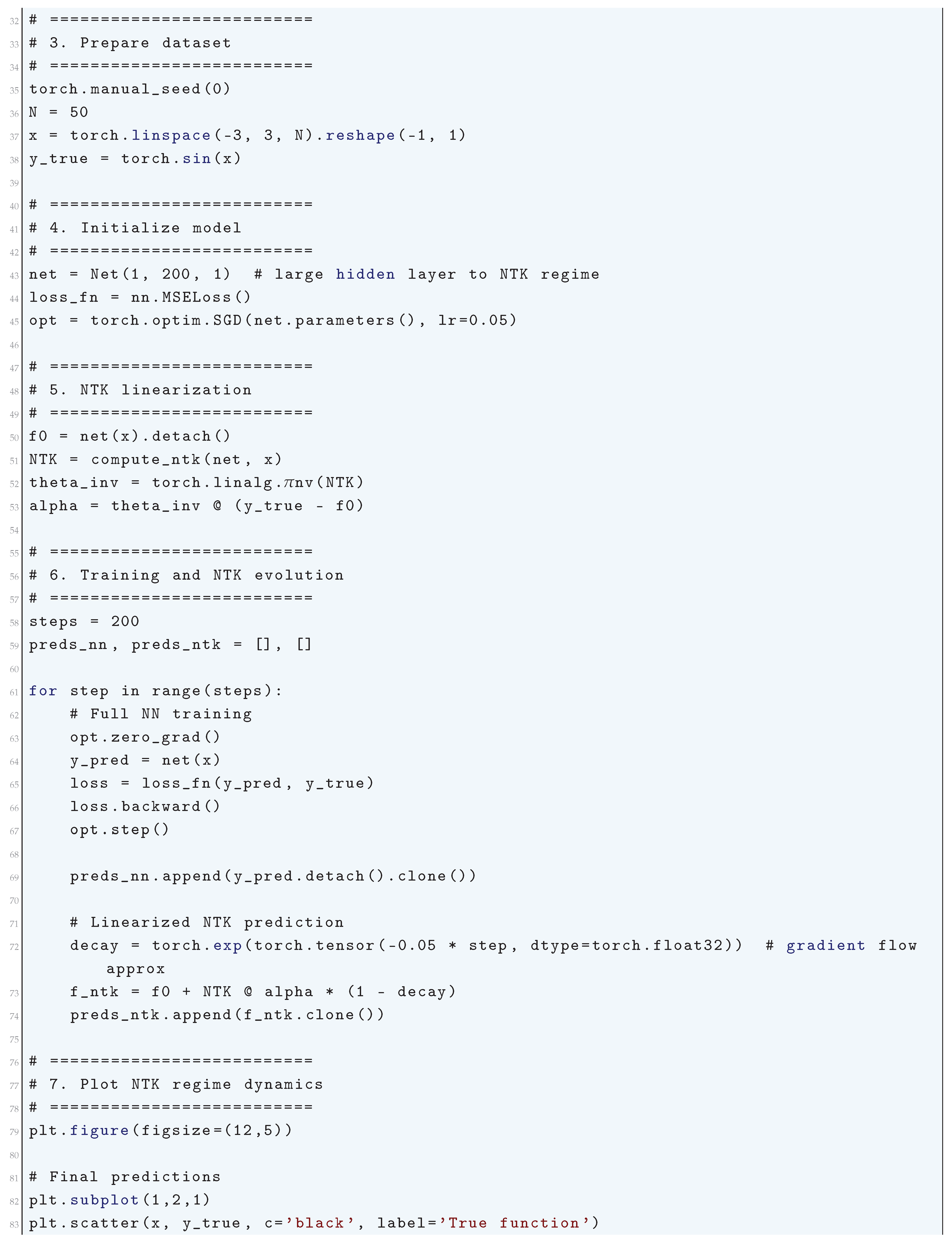
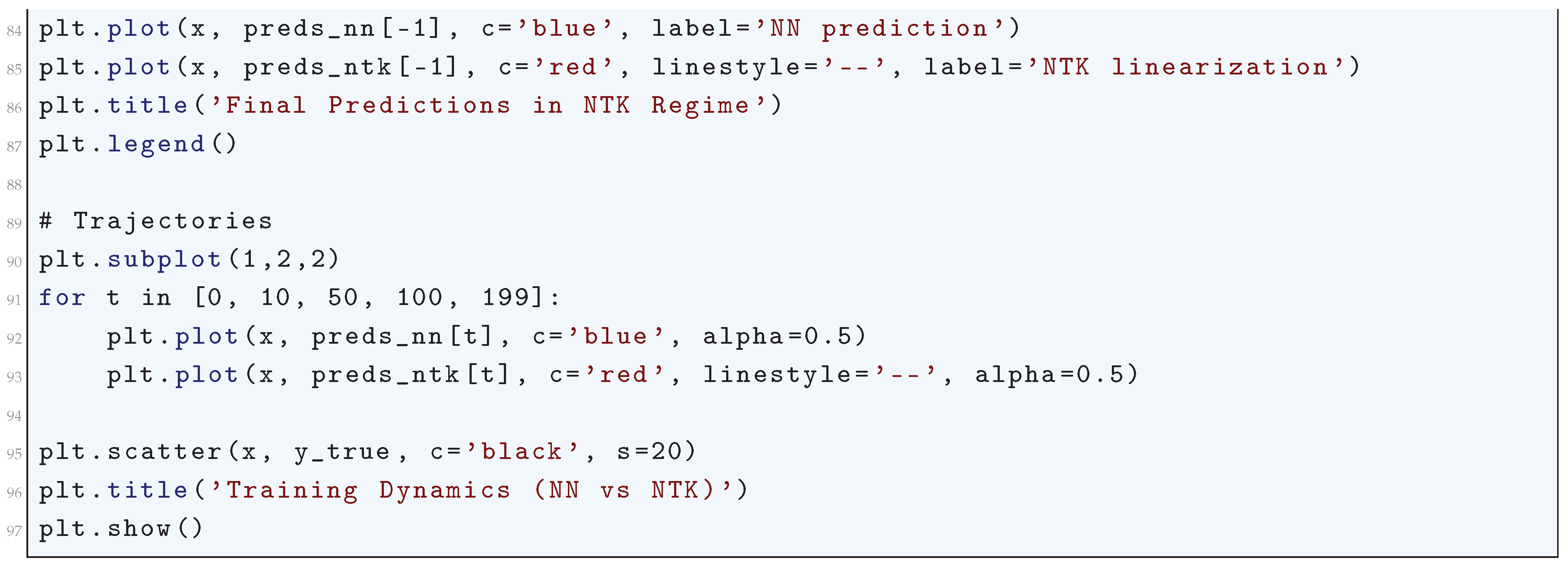
4. Generalization Bounds: PAC-Bayes and Spectral Analysis
The PAC-Bayes framework provides a rigorous mathematical approach to deriving generalization bounds for machine learning models, particularly in stochastic settings. Given a hypothesis space , a prior distribution P over (encoding initial beliefs before observing data), and a posterior distribution Q (learned from data), the PAC-Bayes theorem bounds the expected generalization error. Let denote the true risk of hypothesis and its empirical risk on a sample S of size m. The key PAC-Bayes bound states that, with probability at least over the draw of S, the following holds for all posteriors Q:
where is the Kullback-Leibler divergence between Q and P. This bound balances empirical performance and the complexity of the posterior relative to the prior, ensuring generalization when the learned distribution Q does not deviate excessively from P. The theorem is particularly useful in Bayesian deep learning and stochastic optimization, where Q is often taken as a Gaussian perturbation of a deterministic model.
Spectral analysis examines generalization through the lens of the loss landscape and the eigenspectrum of the Hessian or the Neural Tangent Kernel (NTK). Let be the Hessian of the loss at a local minimum, and let denote its eigenvalues. The effective dimensionality of the solution, which influences generalization, can be characterized by the ratio of the trace to the largest eigenvalue:
Sharp minima, associated with poor generalization, correspond to large relative to the trace, while flat minima (with smaller ) generalize better. Additionally, the NTK’s eigenspectrum determines the speed of gradient descent convergence and the stability of learning dynamics. Let be the NTK at initialization; its eigenvalue decay rate governs how quickly different modes of the target function are learned. If has a rapidly decaying spectrum, high-frequency components (corresponding to small eigenvalues) are learned slowly, leading to implicit regularization. The generalization error can be bounded in terms of the NTK’s eigendecomposition, linking spectral properties to model performance. This approach provides a mechanistic understanding of why overparameterized models generalize despite their capacity to overfit.
4.1. PAC-Bayes Formalism
4.1.1. Literature Review of PAC-Bayes Formalism
McAllester (1999) [99] introduced the PAC-Bayes bound, a fundamental theorem that provides generalization guarantees for Bayesian learning models. He established a trade-off between complexity and empirical risk, serving as the theoretical foundation for modern PAC-Bayesian analysis. Catoni (2007) [100] in his book rigorously extended the PAC-Bayes framework by linking it with information-theoretic and statistical mechanics concepts and introduced exponential and Gibbs priors for learning, improving PAC-Bayesian bounds for supervised classification. Germain et. al. (2009) [101] applied PAC-Bayes theory to linear classifiers, including SVMs and logistic regression. They demonstrated that PAC-Bayesian generalization bounds are tighter than classical Vapnik-Chervonenkis (VC) dimension bounds. Seeger (2002) [102] extended PAC-Bayes bounds to Gaussian Process models, proving tight generalization guarantees for Bayesian classifiers. He laid the groundwork for probabilistic kernel methods. Alquier et. al. (2006) [103] connected variational inference and PAC-Bayes bounds, proving that variational approximations can preserve generalization guarantees of PAC-Bayesian bounds. Dziugaite and Roy (2017) [104] gave one of the first applications of PAC-Bayes to deep learning. They derived nonvacuous generalization bounds for stochastic neural networks, bridging theory and practice. Cox and Ghosh (2022) [54] introduce an analogue of the Mertens function that exhibits similar oscillatory behavior, analyze its properties using Shapiro’s theorem, generalized Dirichlet products, and generalized Möbius inversion, thereby offering new insights into the analytic structure underlying Mertens-type functions. Rivasplata et. al. (2020) [106] provided novel PAC-Bayes bounds that improve over existing guarantees, making PAC-Bayesian bounds more practical for modern ML applications. Lever et. al. (2013) [107] explored data-dependent priors in PAC-Bayes theory, showing that adaptive priors lead to tighter generalization bounds. Rivasplata et. al. (2018) [108] introduced instance-dependent priors, improving personalized learning and making PAC-Bayesian methods more useful for real-world machine learning problems. Lindemann et. al. (2024) [109] integrated PAC-Bayes theory with conformal prediction to improve formal verification in control systems, demonstrating PAC-Bayes’ relevance to safety-critical applications.
4.1.2. Analysis of PAC-Bayes Formalism
The PAC-Bayes formalism is a foundational framework in statistical learning theory, designed to provide probabilistic guarantees on the generalization performance of learning algorithms. By combining principles from the PAC (Probably Approximately Correct) framework and Bayesian reasoning, PAC-Bayes delivers bounds that characterize the expected performance of hypotheses drawn from posterior distributions, given a finite sample of data. This document presents an extremely rigorous and mathematically precise description of the PAC-Bayes formalism, emphasizing its theoretical constructs and implications.
At the core of the PAC-Bayes formalism lies the ambition to rigorously quantify the generalization ability of hypotheses based on their performance on a finite dataset , where represents the underlying, and typically unknown, data distribution. The PAC framework, which was originally designed to provide high-confidence guarantees on the true risk
is enriched in PAC-Bayes by incorporating principles from Bayesian reasoning. This integration allows for bounds not just on individual hypotheses but on distributions Q over , yielding a sophisticated characterization of generalization that inherently accounts for the variability and uncertainty in the hypothesis space. There are some Mathematical Constructs: True and Empirical Risks. The true risk , as defined by the expected loss, is typically inaccessible due to the unknown nature of . Instead, the empirical risk
serves as a computable proxy. The key question addressed by PAC-Bayes is: How does relate to , and how can we bound the deviation probabilistically? For a distribution Q over , these risks are generalized as:
This generalization is pivotal because it allows the analysis to transcend individual hypotheses and consider probabilistic ensembles, where represents a posterior belief over the hypothesis space conditioned on the observed data.
We now need to discuss how Prior and Posterior Distributions encode knowledge and complexity. The prior P is a fixed distribution over that reflects pre-data assumptions about the plausibility of hypotheses. Crucially, P must be independent of S to avoid biasing the bounds. The posterior Q, however, is data-dependent and typically chosen to minimize a combination of empirical risk and complexity. This choice is guided by the PAC-Bayes inequality, which regularizes Q via its Kullback-Leibler (KL) divergence from P:
The KL divergence quantifies the informational cost of updating P to Q, serving as a penalty term that discourages overly complex posteriors. This regularization is critical in preventing overfitting, ensuring that Q achieves a balance between data fidelity and model simplicity.
Let’s derive the PAC-Bayes Inequality: Probabilistic and Information-Theoretic Foundations. The derivation of the PAC-Bayes inequality hinges on a combination of probabilistic tools and information-theoretic arguments. A central step involves applying a change of measure from P to Q, leveraging the identity:
This allows the incorporation of Q into bounds that originally apply to fixed h. By analyzing the moment-generating function of deviations between and , and applying Hoeffding’s inequality to the empirical loss, we arrive at the following bound for any Q and P, with probability at least :
The generalization bound is therefore given by:
where quantifies the divergence between the posterior Q and prior P.
This bound is remarkable because it explicitly ties the true risk to the empirical risk , the KL divergence, and the sample size m. The PAC-Bayes bound encapsulates three competing forces: the empirical risk , the complexity penalty , and the confidence term . This interplay reflects a fundamental trade-off in learning:
- Empirical Risk: captures how well the posterior Q fits the training data.
- Complexity: The KL divergence ensures that Q remains close to P, discouraging overfitting and promoting generalization.
- Confidence: The term shrinks with increasing sample size, tightening the bound and enhancing reliability.
The KL term also introduces an inherent regularization effect, penalizing hypotheses that deviate significantly from prior knowledge. This aligns with Occam’s Razor, favoring simpler explanations that are consistent with the data.
There are several extensions and Advanced Applications of Pac-Bayes Formalism. While the classical PAC-Bayes framework assumes i.i.d. data, recent advancements have generalized the theory to handle structured data, such as in time-series and graph-based learning. Furthermore, alternative divergence measures, like Rényi divergence or Wasserstein distance, have been explored to accommodate scenarios where KL divergence may be inappropriate. In practical settings, PAC-Bayes bounds have been instrumental in analyzing neural networks, Bayesian ensembles, and stochastic processes, offering theoretical guarantees even in high-dimensional, non-convex optimization landscapes.
4.1.2.1 Python Code to Generate Figure 36, Figure 37, and Figure 38 Illustrating PAC-Bayes Bound vs. Sample Size
The Python code below produces the Figure 36, Figure 37, and Figure 38 illustrating PAC-Bayes Bound vs. Sample Size.
Figure 36.
PAC-Bayes Bound vs. Sample Size (KL)
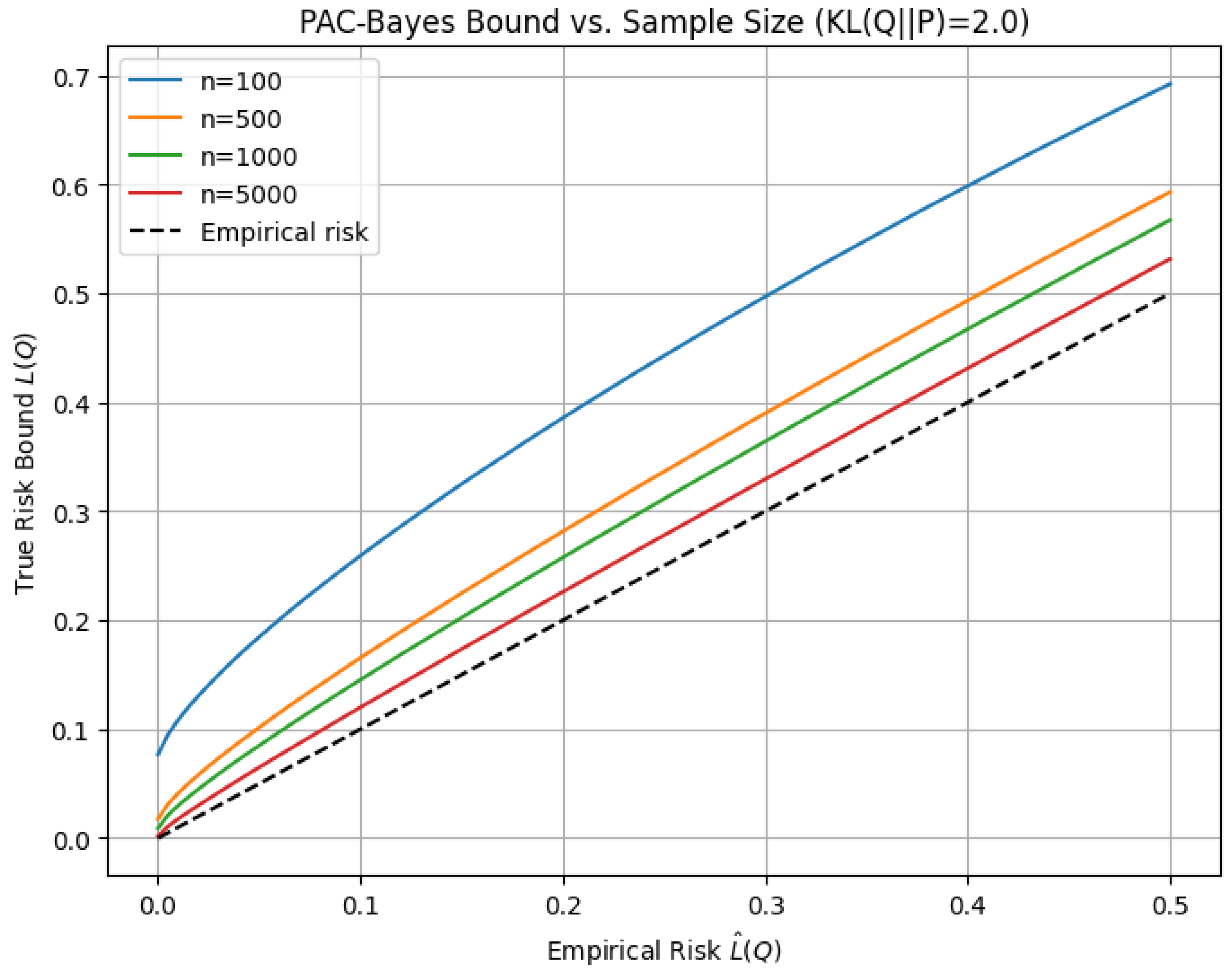
Figure 37.
PAC-Bayes Bound vs. Sample Size (KL)
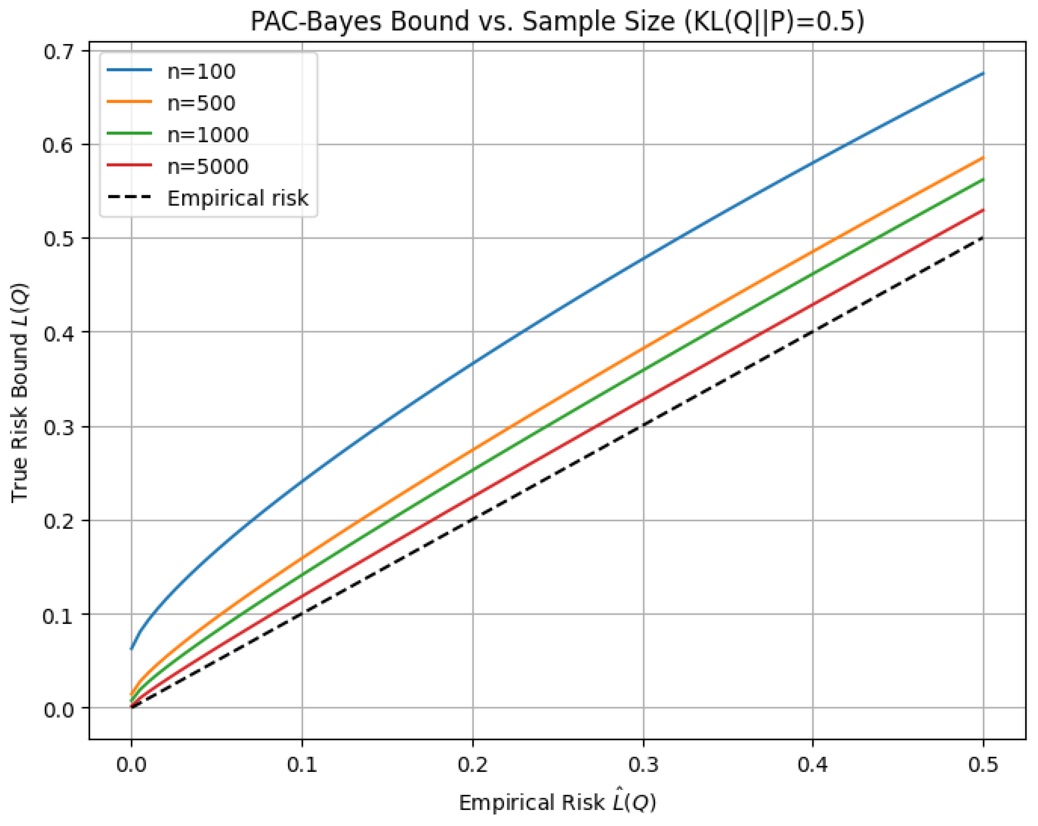
Figure 38.
PAC-Bayes Bound vs. Sample Size (KL)
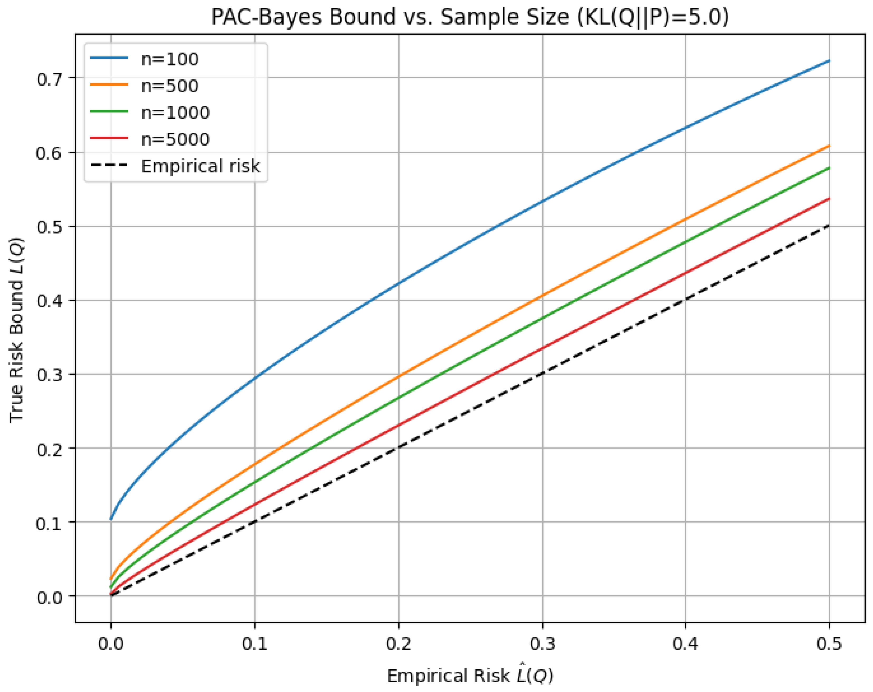
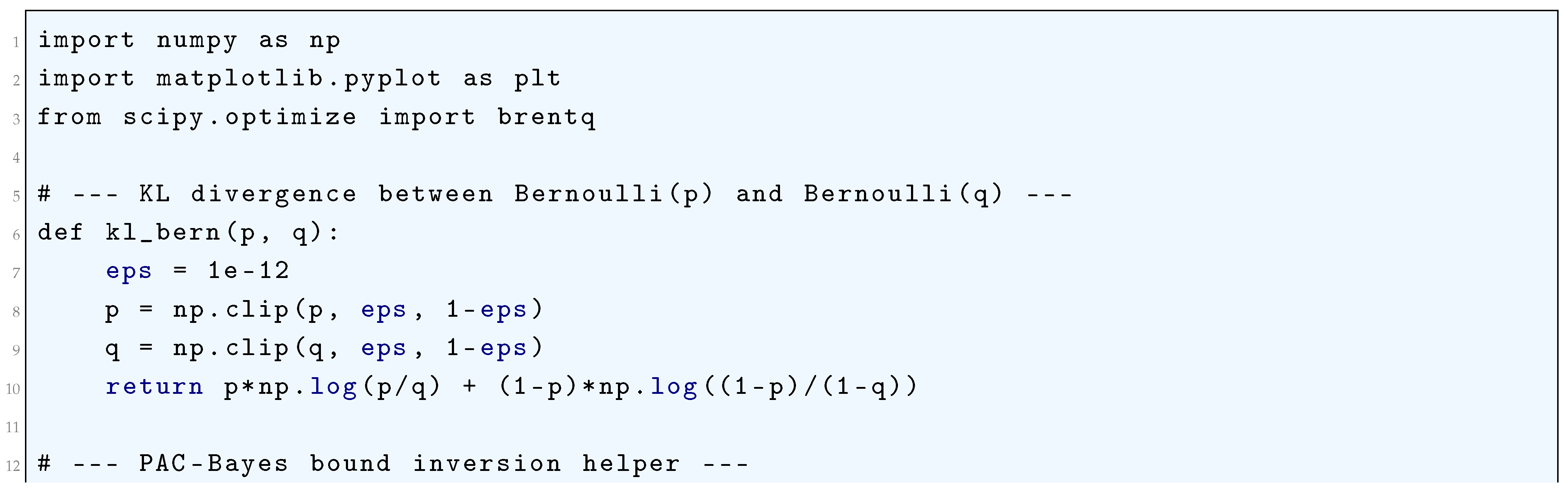
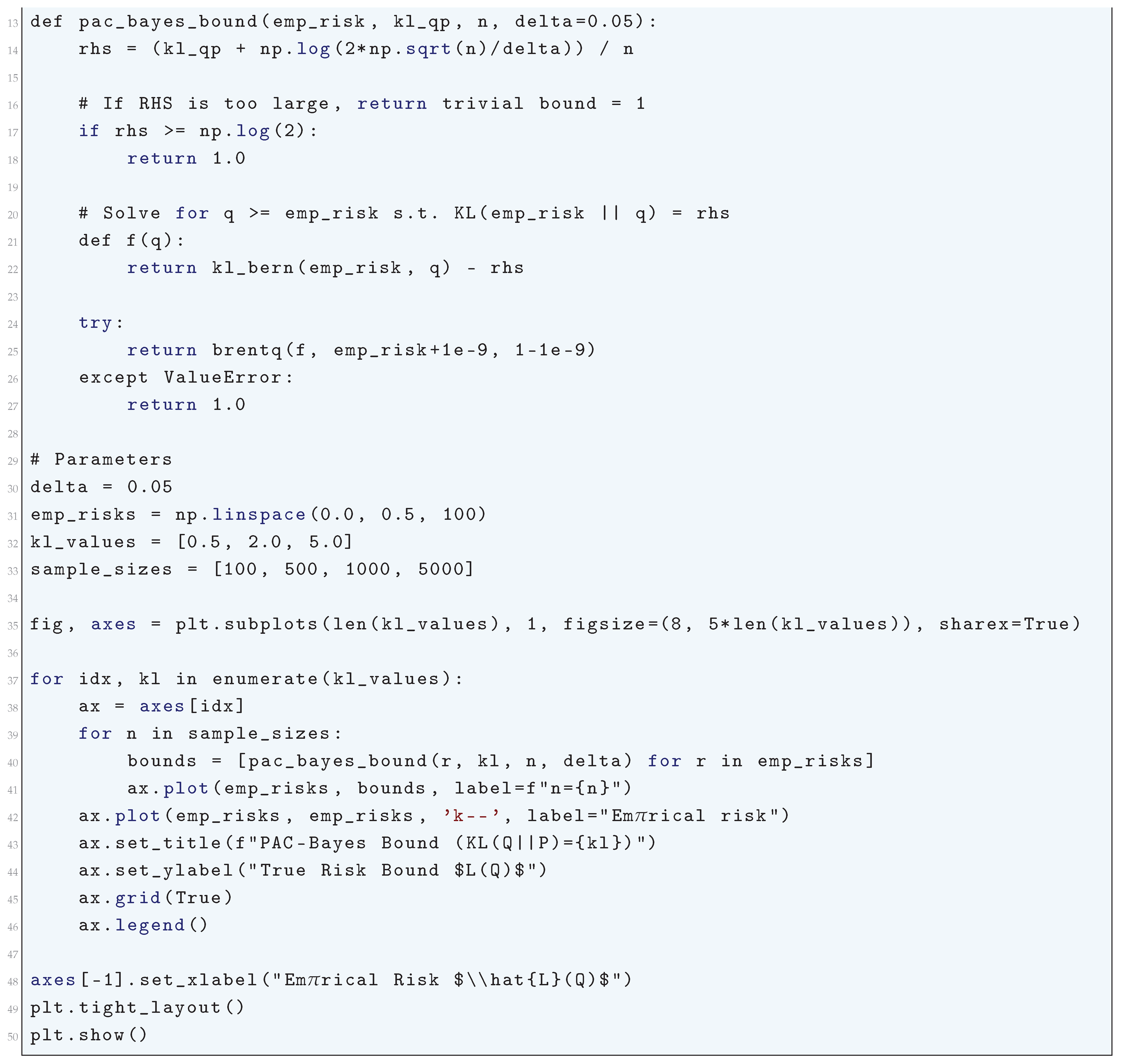
4.1.3. KL Divergence
The Kullback-Leibler (KL) divergence, also known as the relative entropy, is a fundamental concept in information theory, probability theory, and statistics. It quantifies the difference between two probability distributions, measuring the inefficiency of assuming that data is generated from one distribution when it is actually generated from another.
Mathematically, for two discrete probability distributions and defined over a common sample space , the KL divergence is given by
where the logarithm is conventionally taken to be the natural logarithm unless otherwise specified. For continuous probability distributions with probability density functions and , the KL divergence is defined as
The KL divergence can be understood as the expectation of the logarithmic difference between the two distributions, weighted by the true distribution :
Expanding this expectation in integral form,
The first integral represents the entropy of , denoted as
while the second integral represents the cross-entropy between and , given by
Thus, KL divergence can be rewritten as
which represents the additional number of bits required to encode data from when using a coding scheme optimized for instead of . Since the logarithm function is concave, an application of Jensen’s inequality to the function yields the fundamental property
with equality if and only if for all x, which follows from the strict convexity of the logarithm function. Unlike a metric, KL divergence is not symmetric, meaning that in general,
For two multivariate normal distributions and , the KL divergence is given by
where k is the dimension of the Gaussian distribution. This expression reveals that KL divergence accounts for both the difference in mean vectors and the difference in covariance structures.
The KL divergence has a fundamental connection to maximum likelihood estimation (MLE). Given a true data distribution and a parametric model , the parameter that minimizes the KL divergence
is equivalent to the maximum likelihood estimate, since minimizing KL divergence is equivalent to maximizing the log-likelihood function
This follows from the fact that the term does not depend on and is therefore irrelevant for optimization. In Bayesian inference, KL divergence plays a central role in variational inference. Given an intractable posterior , one approximates it with a tractable distribution , where the objective is to minimize
This minimization leads to the Evidence Lower Bound (ELBO),
which is central in modern probabilistic modeling. Moreover, KL divergence is related to mutual information. Given two random variables X and Y with a joint distribution and marginals and , the mutual information is given by
which quantifies the amount of information shared between X and Y. In information geometry, the Fisher information matrix is derived from the second-order expansion of KL divergence,
KL divergence is also connected to the Pinsker inequality,
This establishes KL divergence as a fundamental measure of probability distance in statistical inference and machine learning.
The Kraft–McMillan inequality establishes a necessary and sufficient condition for the existence of a uniquely decodable code with a given set of codeword lengths. For a code over a D-ary alphabet to be uniquely decodable, the codeword lengths must satisfy the inequality
This inequality is foundational because it directly links the lengths of codewords to a probability distribution. Specifically, if we define , then the Kraft sum condition
implies that can be normalized to form a probability distribution. This provides a formal bridge between the theory of codes and the theory of probability distributions, which is the central domain of information theory measures like the Kullback-Leibler (KL) Divergence.
The KL Divergence, or relative entropy, between two probability distributions P and Q over the same discrete set is defined as
Its importance in data compression is given by the source coding theorem, which states that the expected codeword length of an optimal code for a source with distribution P is bounded by
where is the Shannon entropy. When the code is designed for an incorrect distribution Q, the expected codeword length becomes
The Kraft–McMillan theorem guarantees that for any uniquely decodable code with lengths , there exists a probability distribution
where is the Kraft sum. This allows the lengths to be expressed as
and since , we have
The expected length when using a code optimal for Q on data from P is
Substituting the fundamental relation for a code that meets the Kraft inequality with equality for distribution Q yields
The difference between this suboptimal expected length and the entropy lower bound is
This simplifies directly to , as
Therefore, the KL Divergence quantifies the inefficiency, in bits or nats, incurred by using a code designed for a distribution Q when the true data-generating distribution is P. The mathematical rigor of this relationship is entirely contingent upon the Kraft–McMillan theorem, which provides the necessary condition
that legitimizes the interpretation of code lengths as representing a probability distribution, thereby enabling the derivation
for a code that is optimal for Q.
4.1.3.1 Python Code to Generate Figure 39, Figure 40 Illustrating KL Divergence in Bernoulli Random Variables and Figure 41, Figure 42 Illustrating KL Divergence in Gaussian Random Variables
The Python code below produces the Figure 39, Figure 40 illustrating KL Divergence in Bernoulli Random Variables and Figure 41, Figure 42 illustrating KL Divergence in Gaussian Random Variables.
Figure 39.
KL Divergence between Bernoulli(p) and Bernoulli(q)
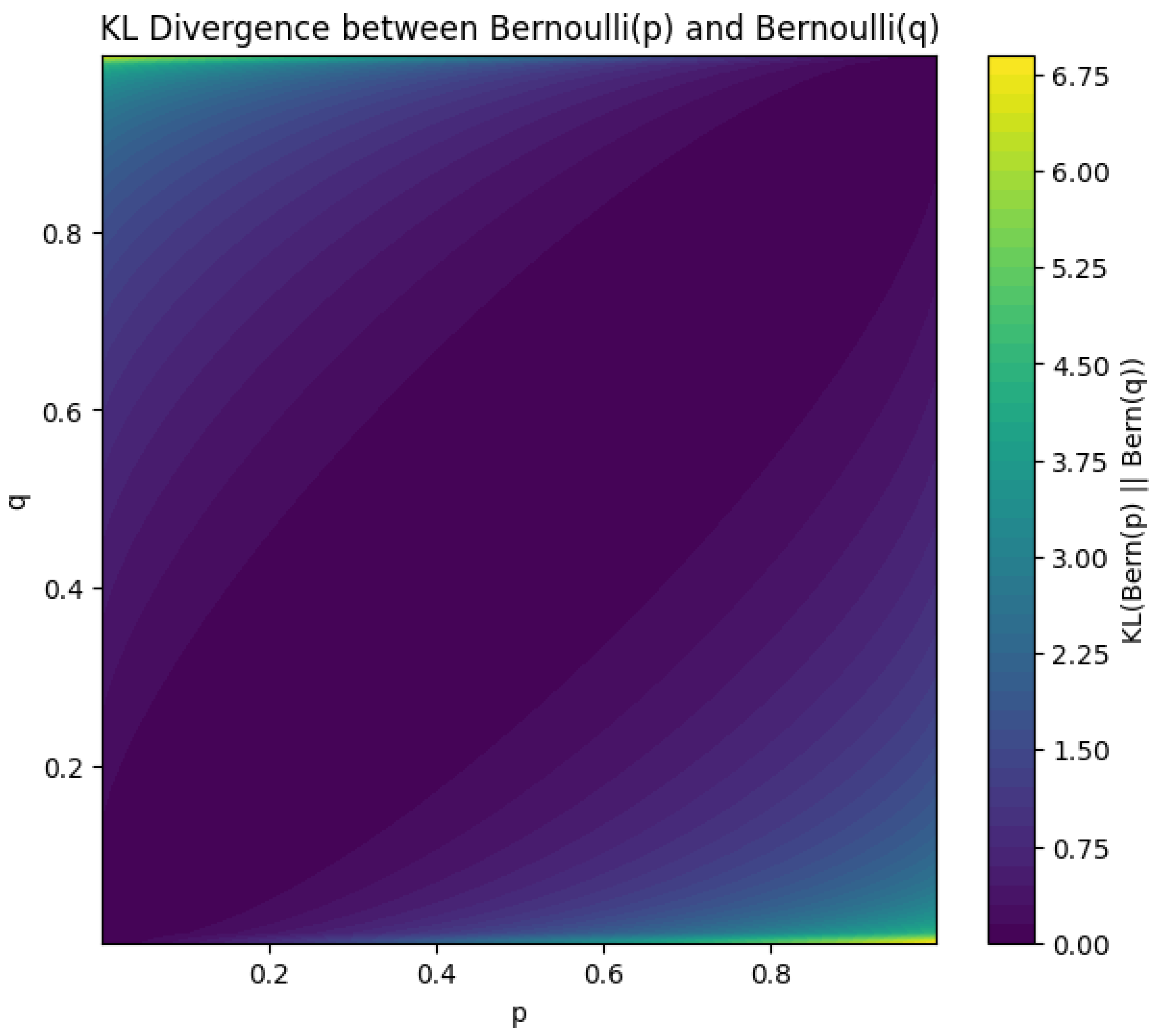
Figure 40.
KL Divergence as function of q for fixed p
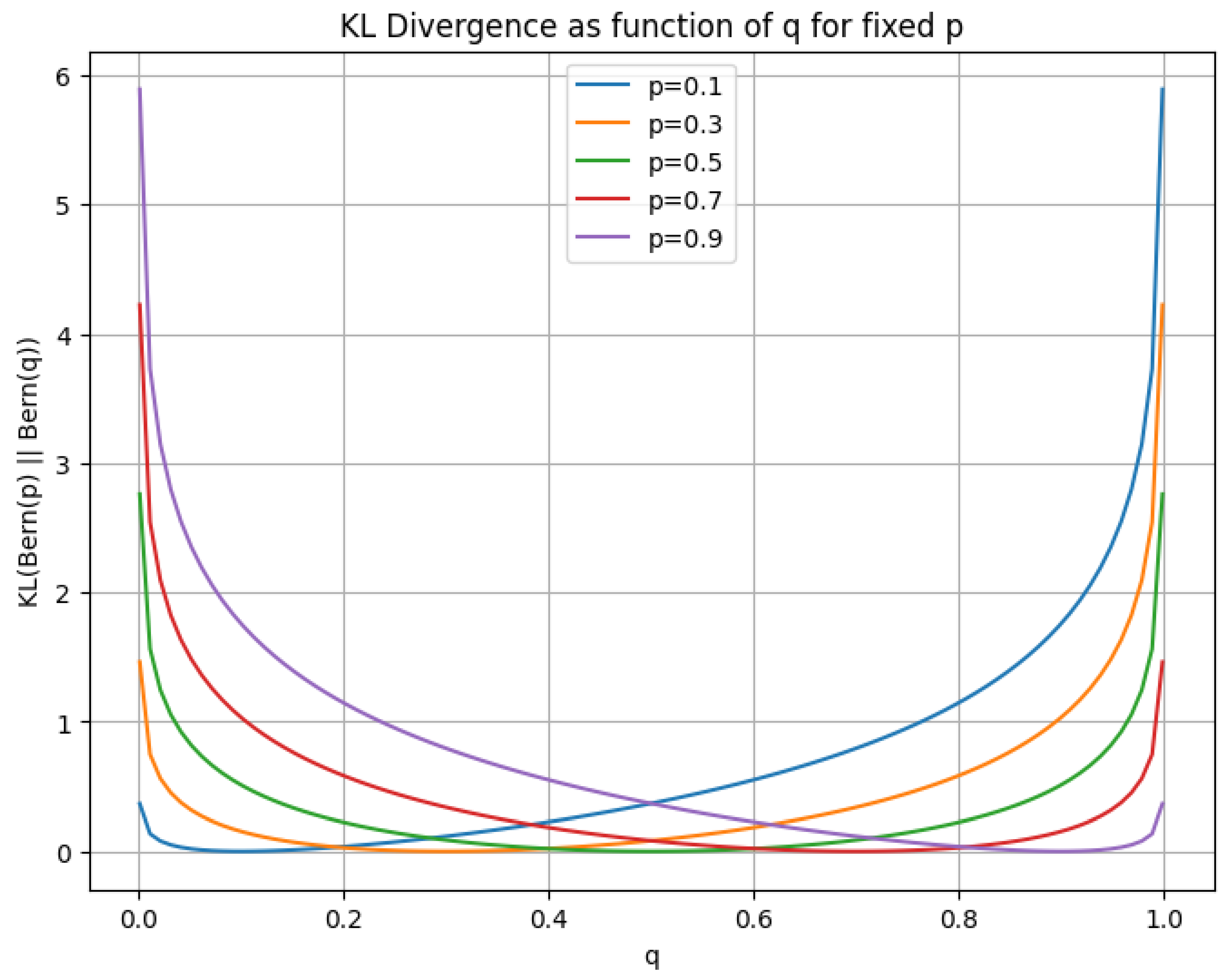
Figure 41.
Gaussian KL Divergence (equal variances)
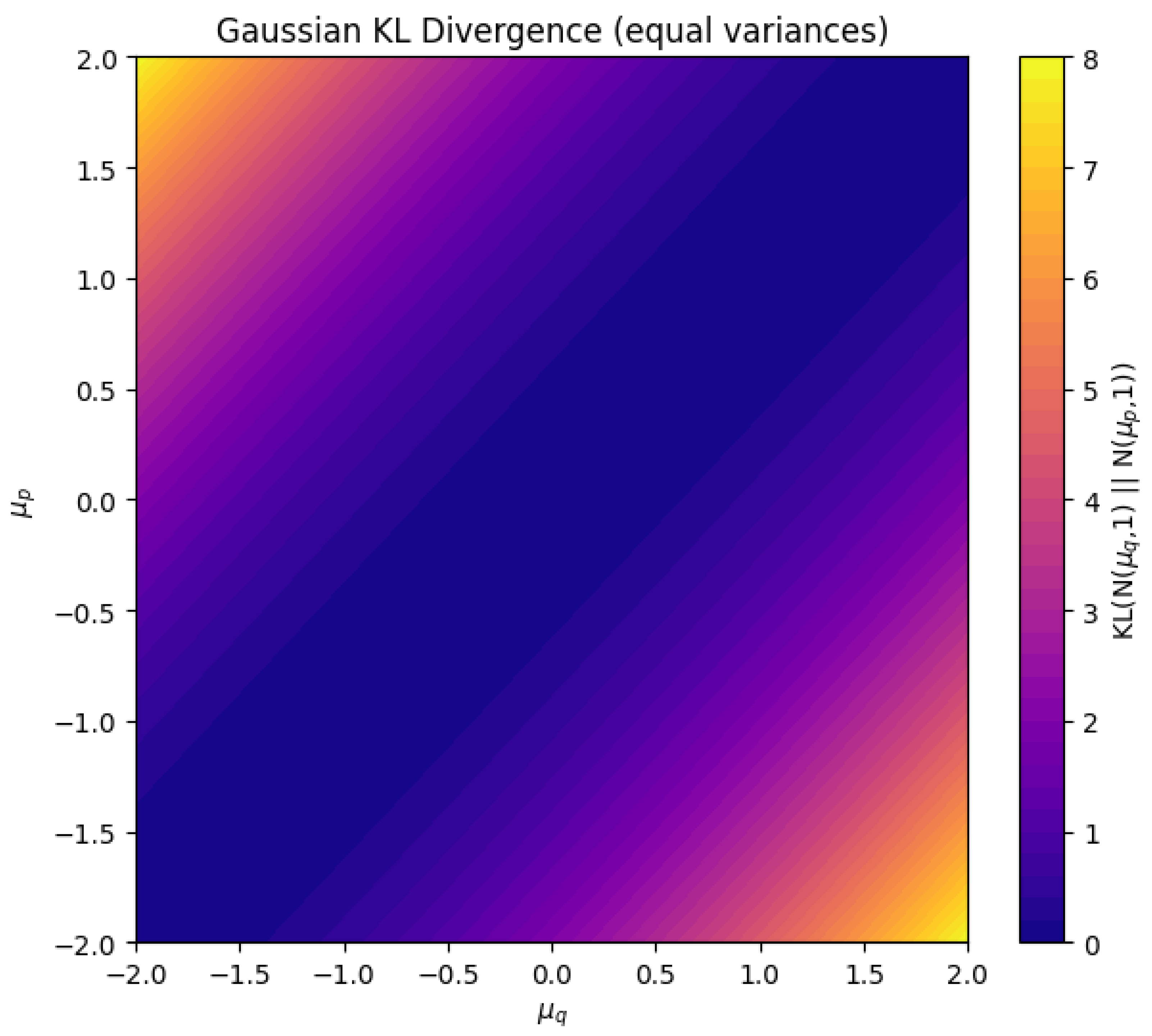
Figure 42.
Gaussian KL Divergence vs ()
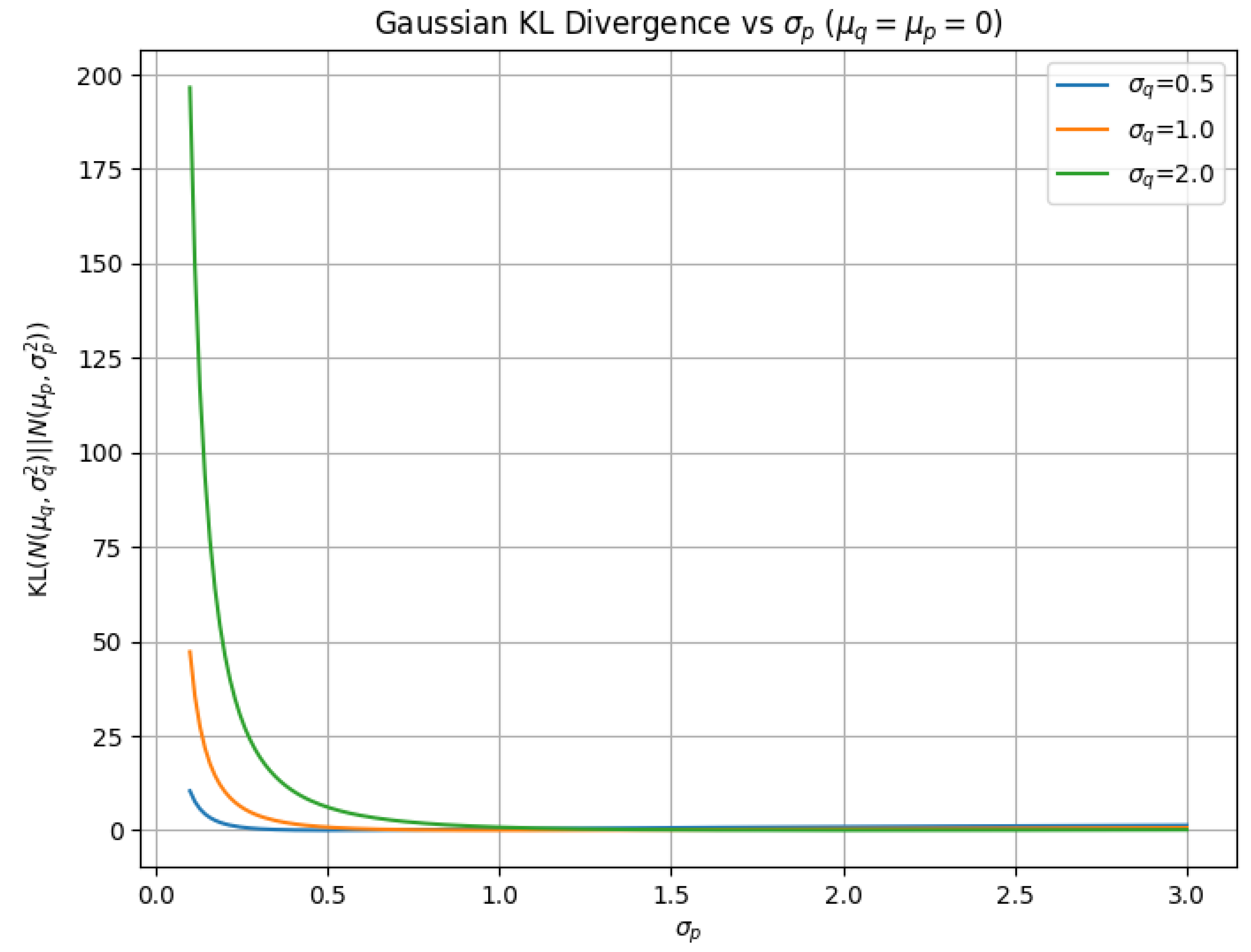
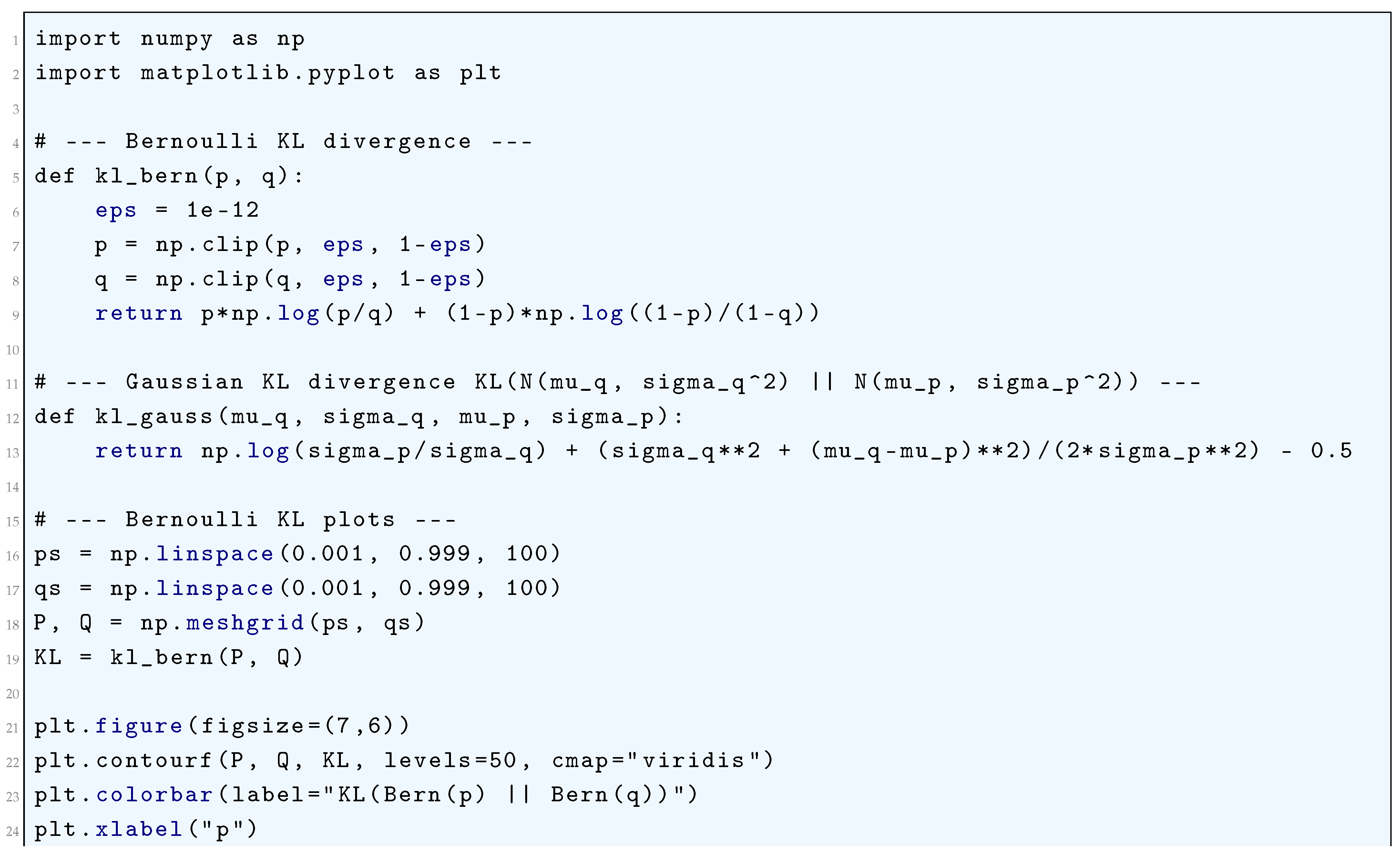
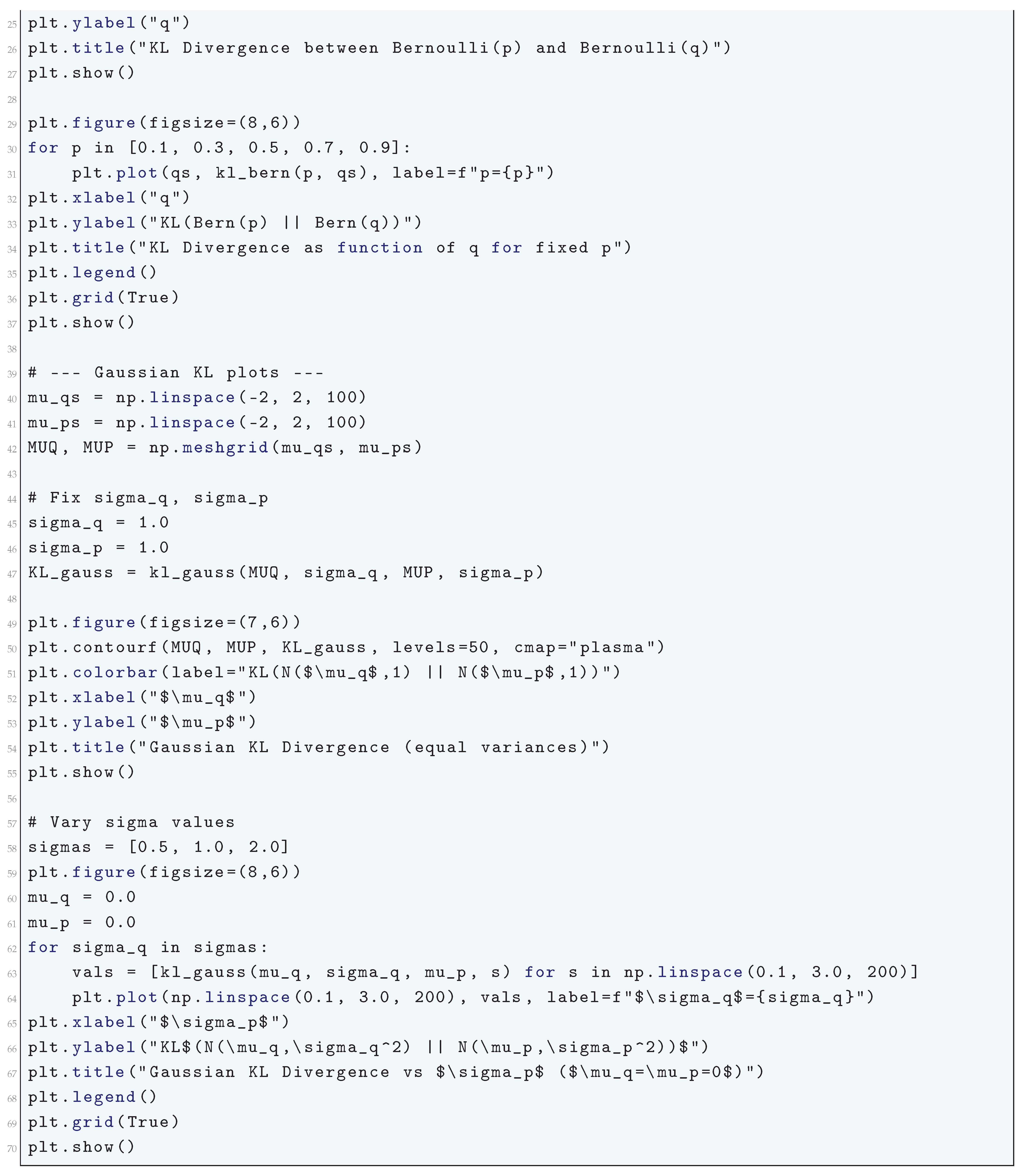
4.1.4. Rényi Divergence
The Rényi divergence is a parametric family of divergences that generalizes the Kullback-Leibler (KL) divergence and provides a broader measure of dissimilarity between probability distributions.
Given two probability distributions P and Q defined on a measurable space , the Rényi divergence of order (for and ) is defined as
where and denote the Radon-Nikodym derivatives (i.e., probability density functions) of P and Q with respect to a common reference measure . That is,
For the case where P and Q are discrete distributions supported on a finite or countable set , the Rényi divergence takes the form
Equivalently, it can be expressed using expectation notation as
This expression shows that Rényi divergence is a moment-based measure of dissimilarity between P and Q, generalizing the standard KL divergence, which is recovered in the limit . To see this, we differentiate
with respect to and apply L’Hôpital’s rule. Explicitly, defining
we compute
Applying the logarithmic derivative, we obtain
demonstrating the convergence to the KL divergence. The Rényi divergence satisfies the following fundamental mathematical properties. It is non-negative,
Additionally, Rényi divergence is a monotonic function of , satisfying
For special values of , Rényi divergence simplifies to various known divergences. When , it becomes
which represents the negative logarithm of the probability mass that Q assigns to the support of P. When , we obtain
which is related to the chi-squared divergence. When , the divergence simplifies to
which measures the worst-case discrepancy between the two distributions. One crucial property of the Rényi divergence is its invariance under transformations. Given a Markov kernel T that maps P and Q to new distributions and , the data-processing inequality states
ensuring that no transformation can increase the divergence between distributions. Rényi divergence also satisfies the joint convexity property: for a mixture of probability distributions and with weights ,
This inequality demonstrates that Rényi divergence behaves well under probabilistic mixing. Another fundamental result is the Pinsker-type bound, which states that for , the Rényi divergence is bounded below by a function of the total variation distance ,
For small , this inequality shows that Rényi divergence behaves quadratically in the deviation between P and Q. Furthermore, the Rényi divergence is closely related to the Chernoff information, which determines the optimal exponent for Bayesian hypothesis testing. The Chernoff information is defined as
which plays a fundamental role in large deviations theory and hypothesis testing.
In summary, the Rényi divergence is a highly versatile and mathematically rich measure of dissimilarity between probability distributions. It generalizes the KL divergence, interpolates between various known divergence measures, satisfies essential properties such as monotonicity and data-processing inequalities, and has deep connections to large deviation theory, statistical estimation, and hypothesis testing.
4.1.4.1 Python Code to Generate Figure 43 and Figure 44 Illustrating Rényi Divergence
Figure 43.
Rényi Divergence between Gaussians vs.
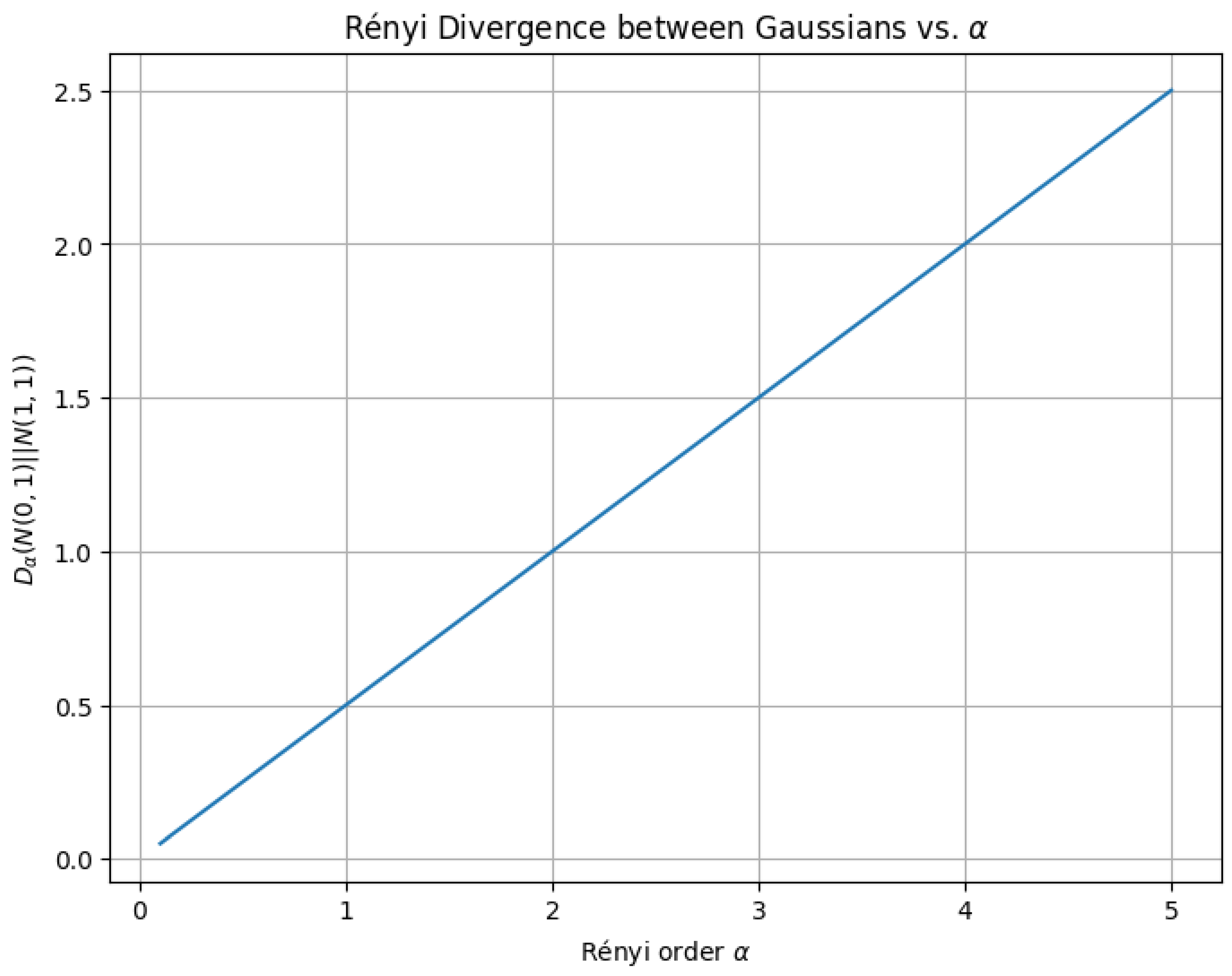
Figure 44.
Rényi Divergence Heatmap ()
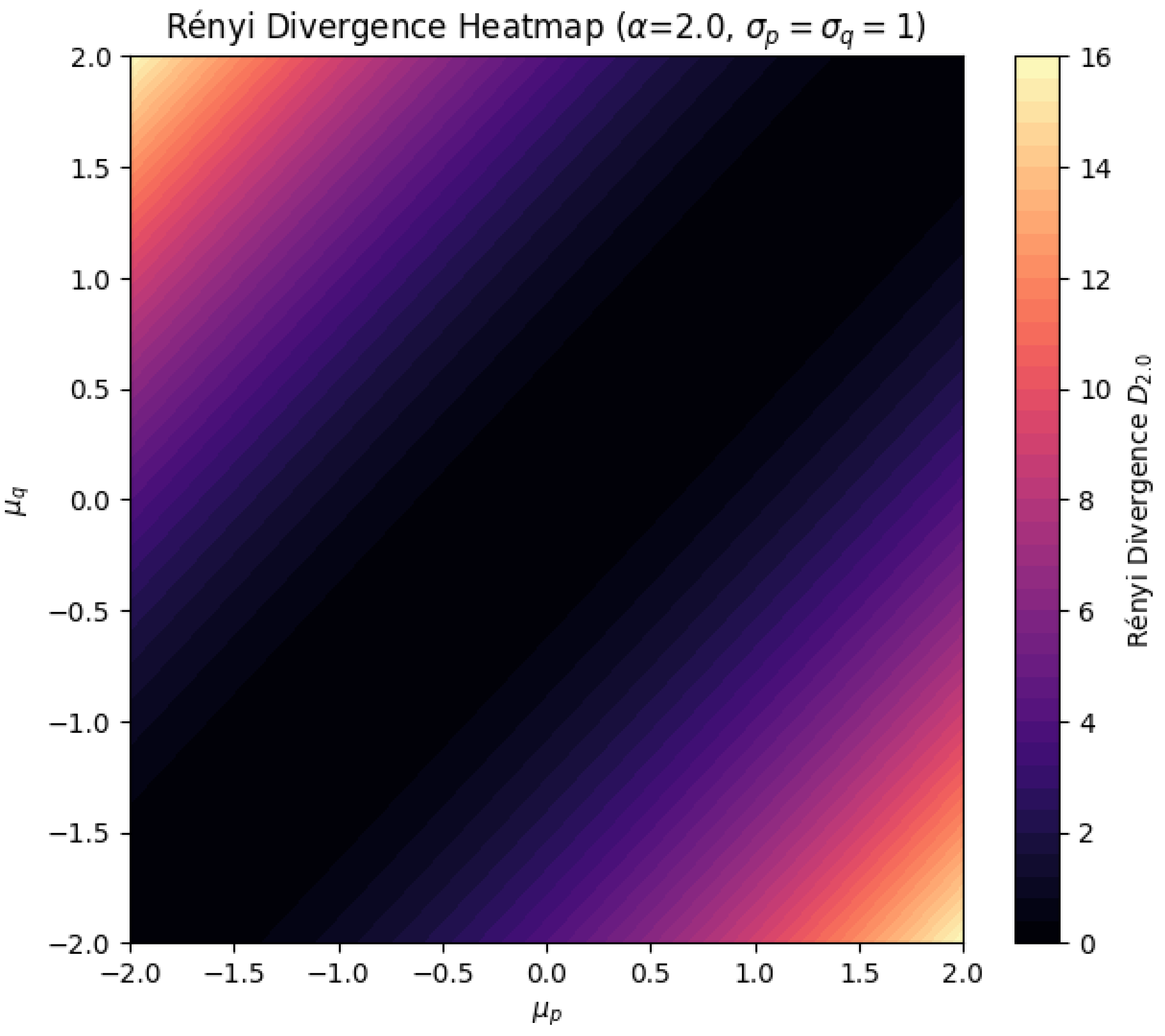
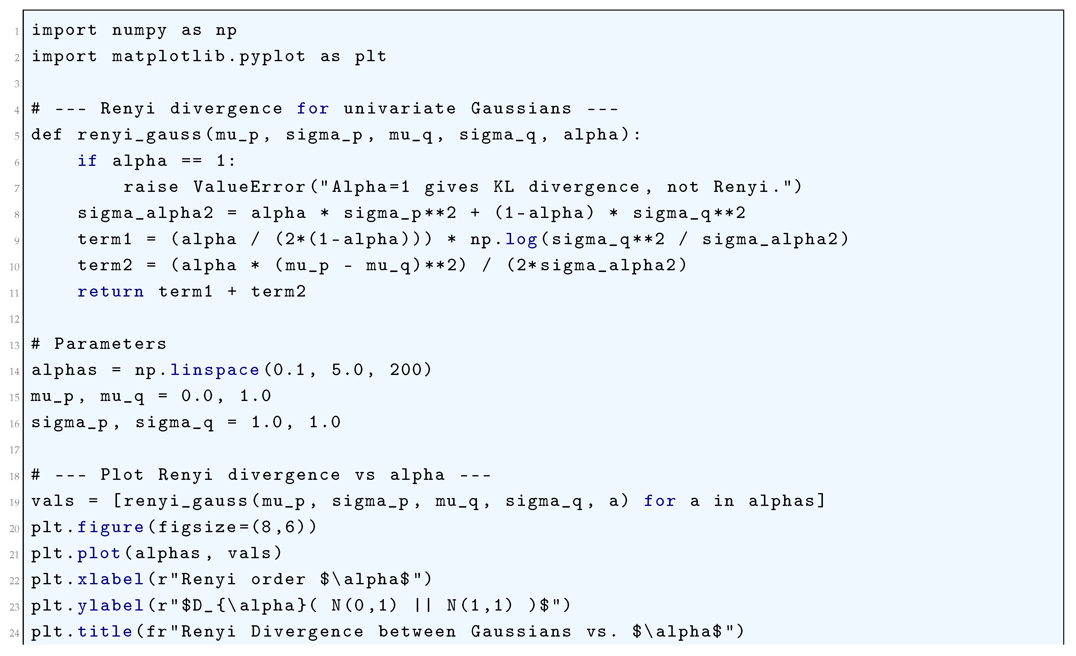
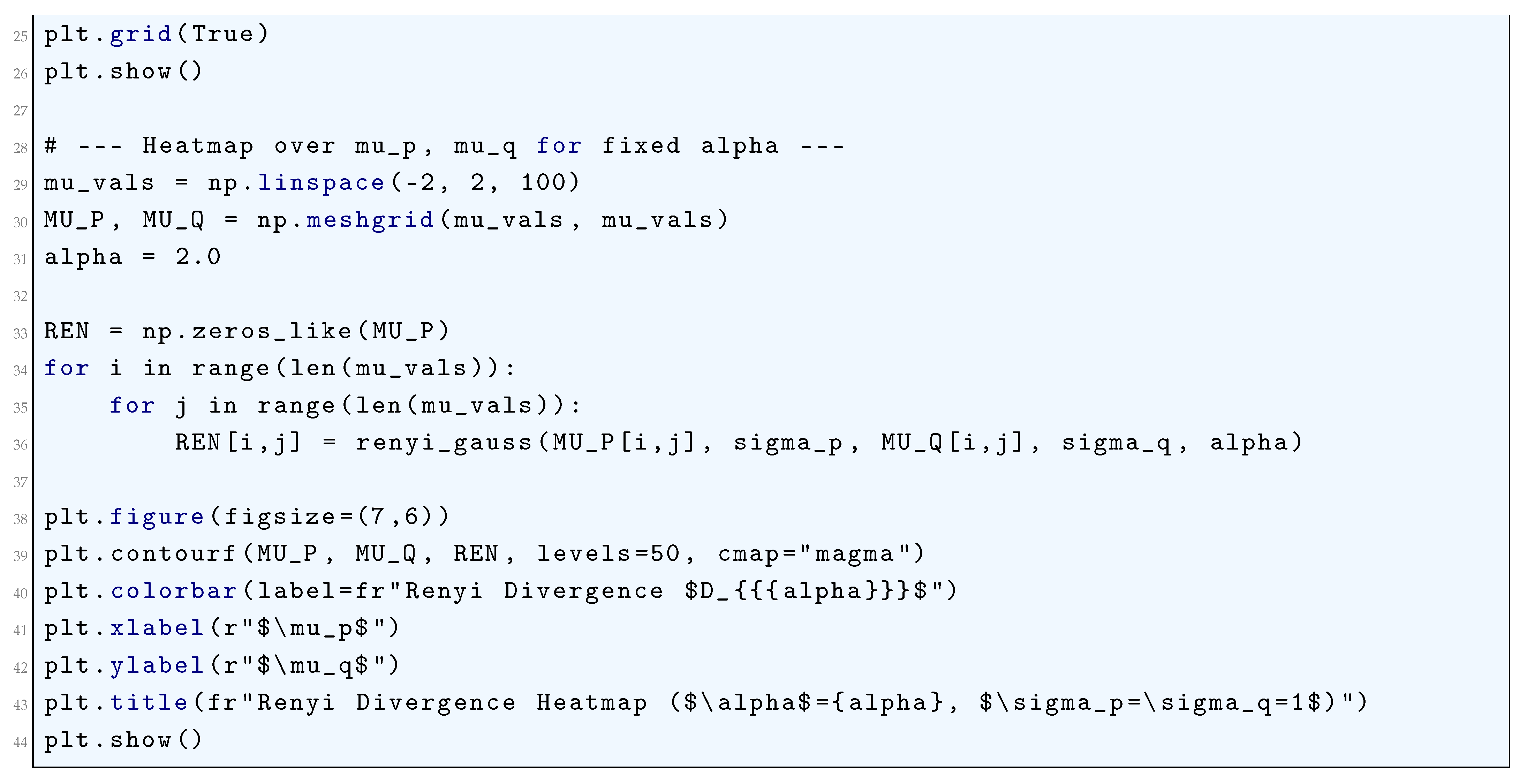
4.1.5. Wasserstein Distance
The Wasserstein distance, also referred to as the Earth Mover’s Distance (EMD), is a fundamental metric in the field of optimal transport theory that rigorously quantifies the distance between two probability measures by determining the minimal cost required to transport one measure into another.
Consider two probability distributions and , defined on a metric space . The Wasserstein distance of order is defined by
where denotes the set of all probability measures on the product space satisfying
This definition arises from the optimal transport problem, originally formulated by Monge in 1781 and later extended by Kantorovich. The Monge formulation seeks a transport map that pushes onto , i.e., satisfies
where denotes the pushforward measure defined by
The Monge formulation minimizes the total transport cost given by
However, the existence of an optimal transport map is highly constrained and may fail in many cases. To overcome this, Kantorovich introduced a relaxation in which transport maps are replaced by probability couplings , leading to the variational problem
This formulation allows for mass splitting, making the problem more tractable and ensuring the existence of minimizers under mild conditions. The dual formulation of the Wasserstein distance is given by
subject to the constraint
For , the Kantorovich-Rubinstein theorem provides an alternative characterization
When , the Wasserstein-1 distance has the closed-form expression
where and are the cumulative distribution functions of and , respectively. For , the squared Wasserstein-2 distance is given by
If and are Gaussian distributions and , then
The Wasserstein distance induces a metric on the space of probability measures, providing a notion of distance that is weaker than total variation but stronger than weak convergence.
Specifically, if in Wasserstein distance, then for any function f satisfying
it holds that
The Wasserstein metric endows the space of probability measures with a Riemannian-like structure, where geodesics are given by McCann interpolation, defined as
For discrete distributions
the Wasserstein distance reduces to a linear programming problem
Computationally, Wasserstein distances are expensive to evaluate, but regularized approximations such as Sinkhorn’s algorithm solve the entropically regularized problem
This approximation allows for efficient computation via iterative updates using the Sinkhorn-Knopp algorithm. The Wasserstein distance plays a crucial role in probability theory, statistics, machine learning, and functional analysis, providing a rigorous mathematical framework for comparing distributions with deep connections to convex geometry, measure theory, and differential geometry.
4.1.5.1 Python Code to Generate Figure 45, Figure 46, and Figure 47 Illustrating Wasserstein Distance
The Python code below produces the Figure 45, Figure 46, and Figure 47 illustrating Wasserstein distance.
Figure 45.
Wasserstein Distance vs Mean Difference ()
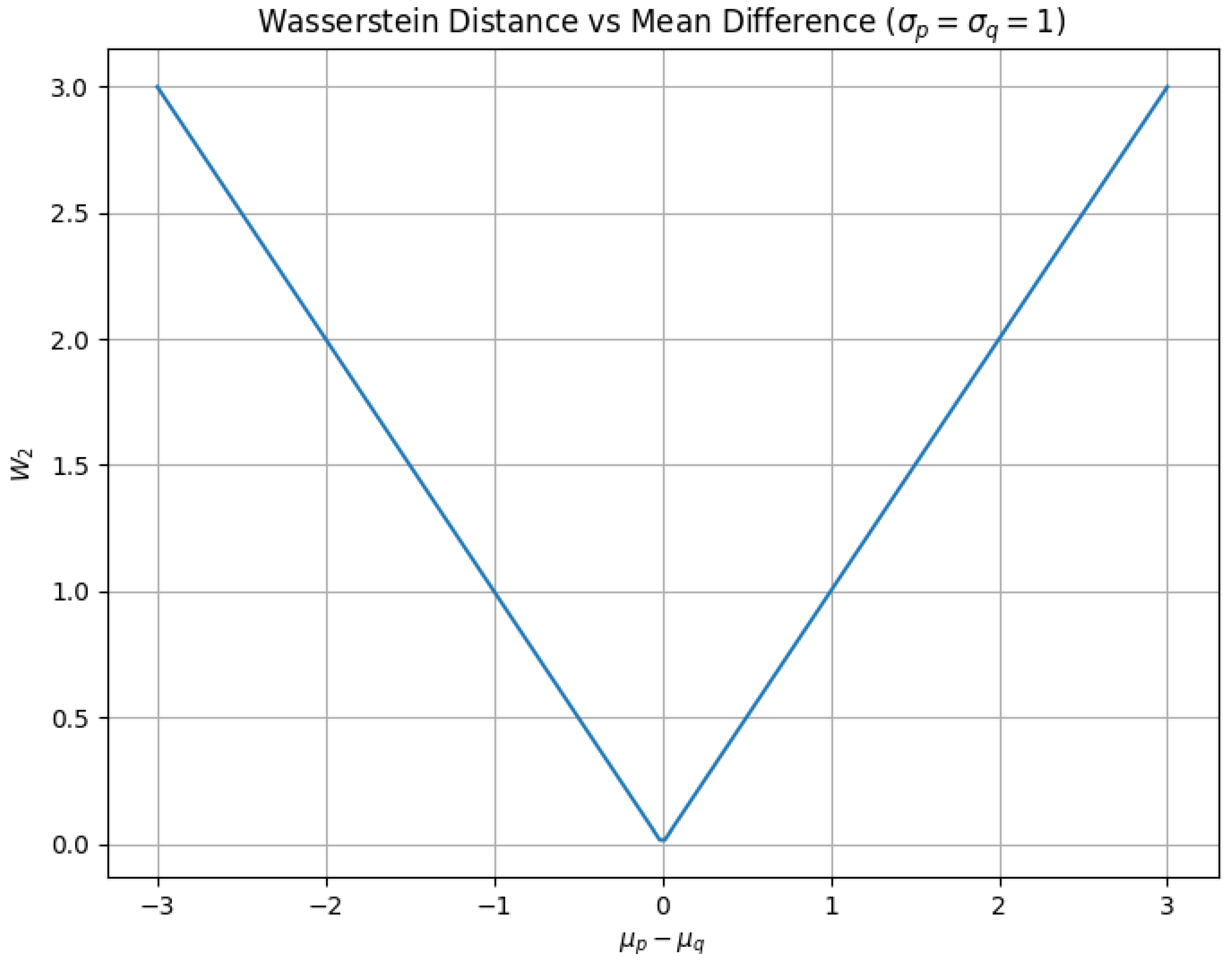
Figure 46.
Wasserstein Distance vs Variance ()
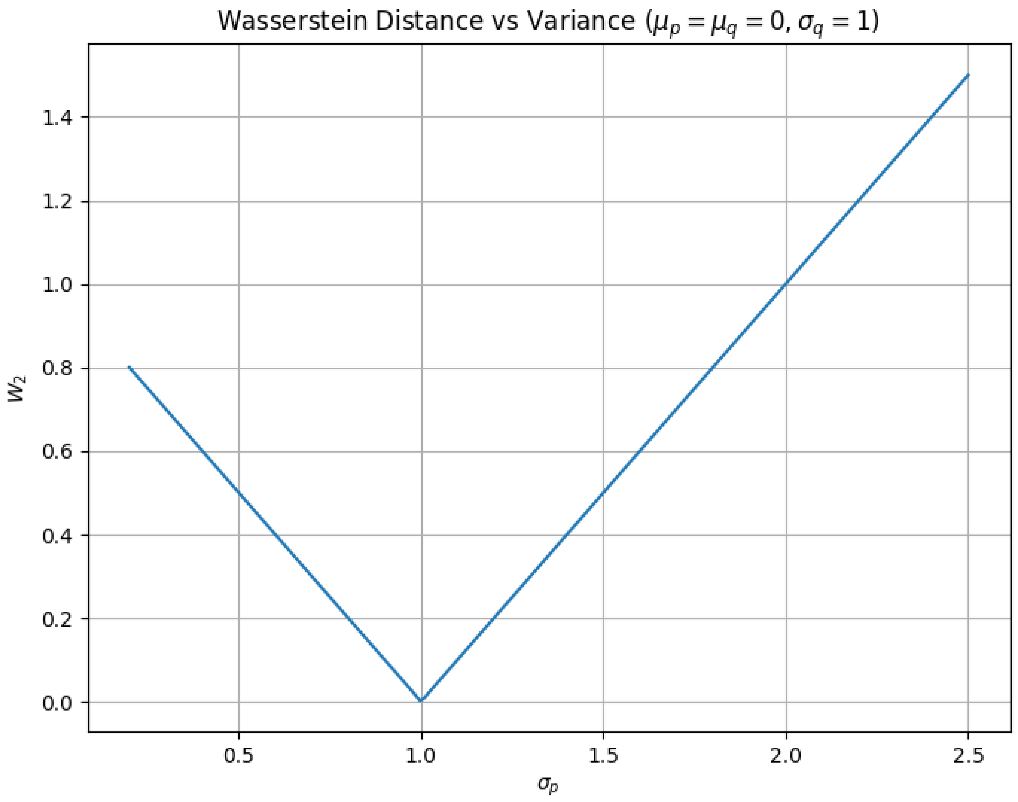
Figure 47.
Wasserstein Distance Heatmap ()
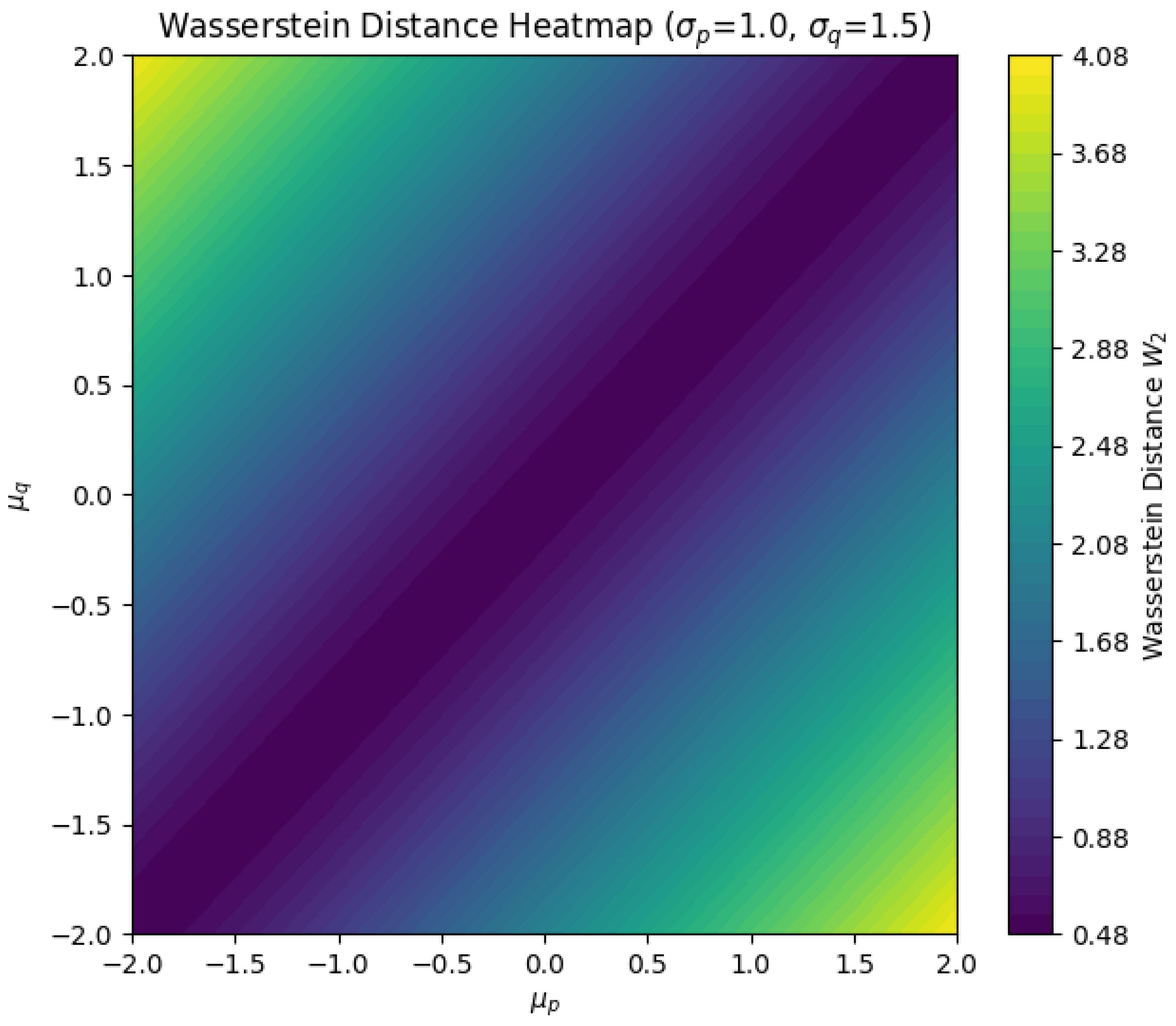
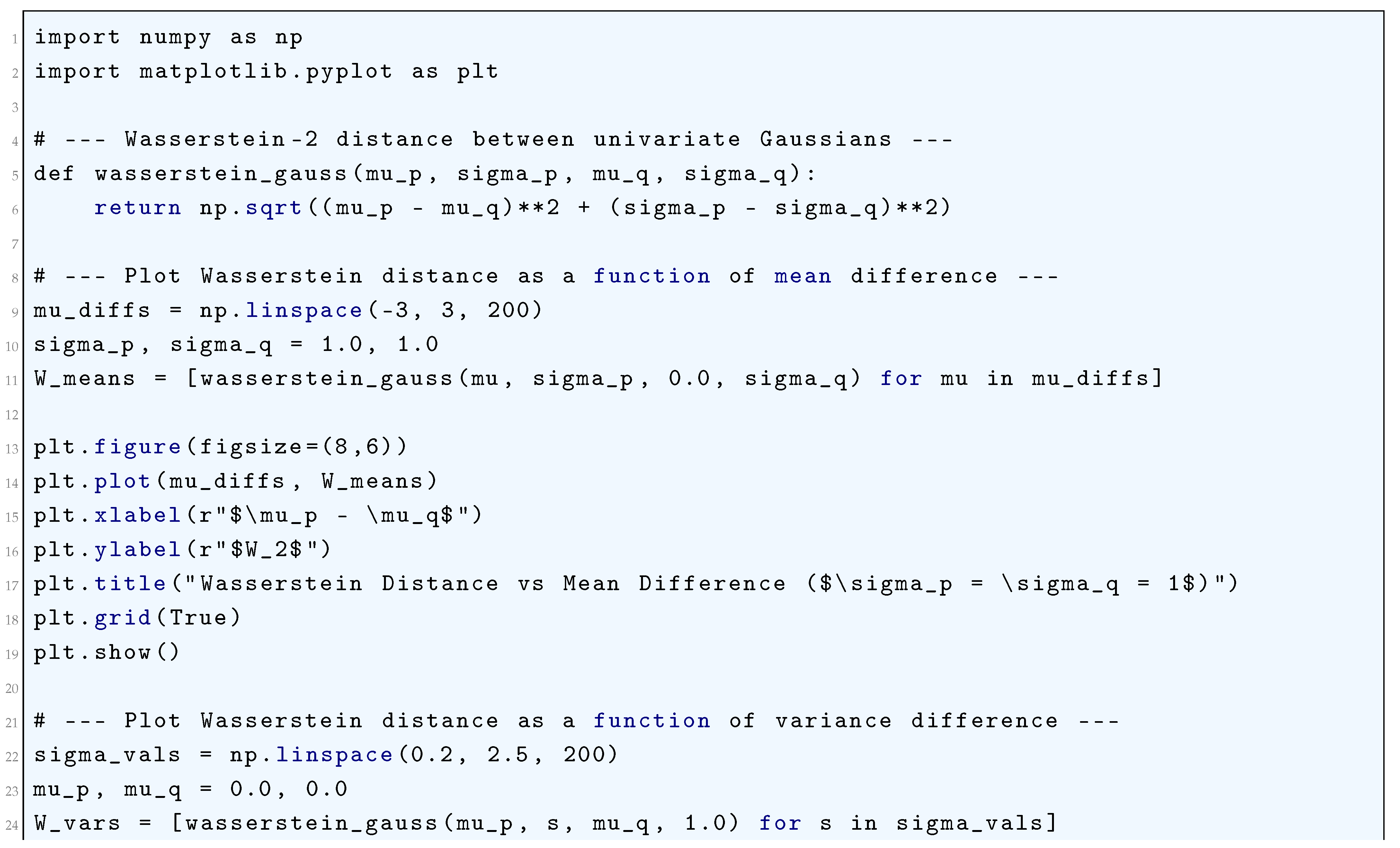
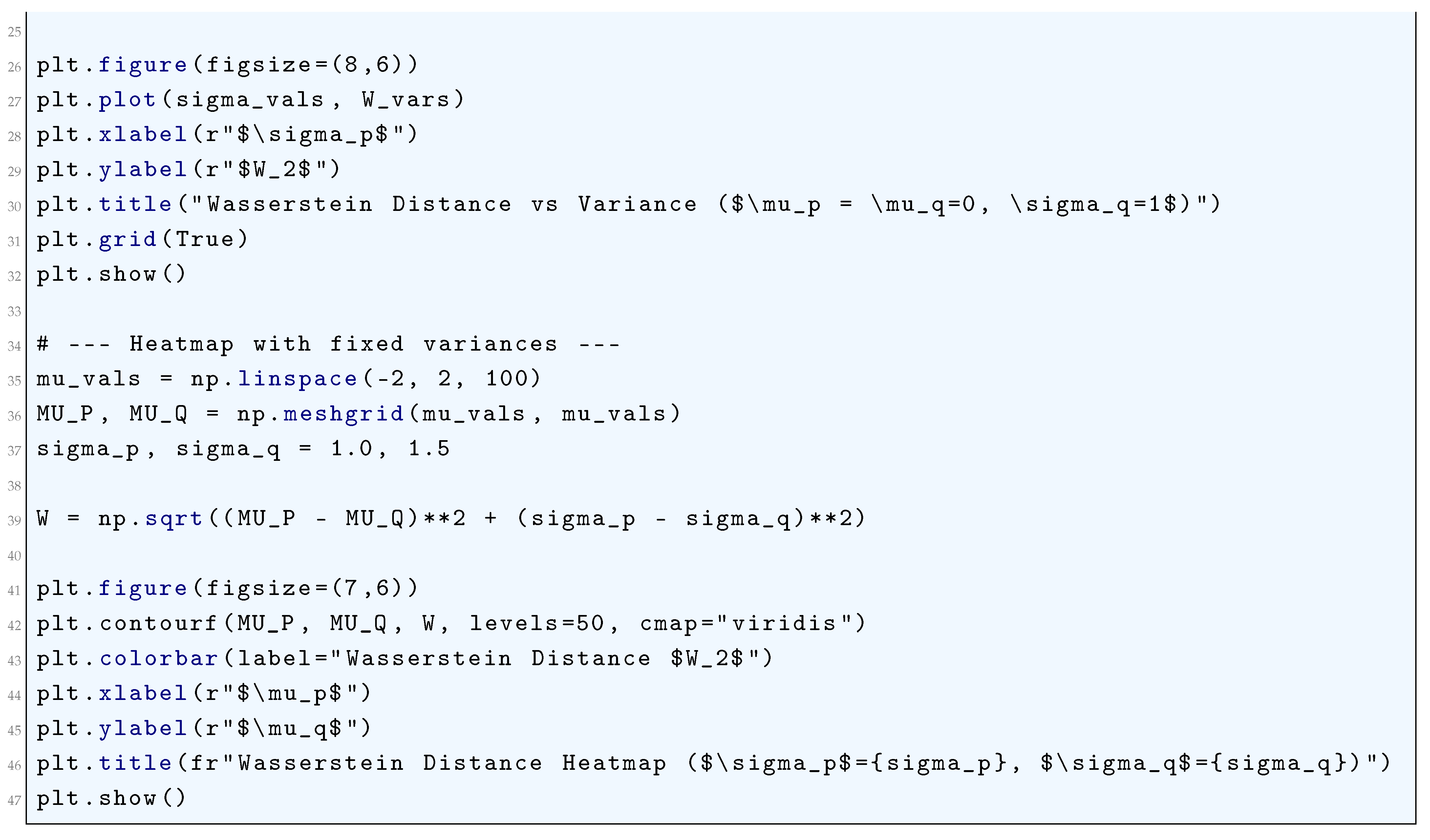
4.2. Spectral Regularization
The concept of spectral regularization, which refers to the preferential learning of low-frequency modes by neural networks before high-frequency modes, emerges from a combination of Fourier analysis, optimization theory, and the inherent properties of deep neural networks. This phenomenon is tightly connected to the functional approximation capabilities of neural networks and can be rigorously understood through the lens of Fourier decomposition and the gradient descent optimization process.
4.2.1. Literature Review of Spectral Regularization
Jin et. al. (2025) [110] introduced a novel confusional spectral regularization technique to improve fairness in machine learning models. The study focuses on the spectral norm of the robust confusion matrix and proposes a method to control spectral properties, ensuring more robust and unbiased learning. It provides insights into how regularization can mitigate biases in classification tasks. Ye et. al. (2025) [111] applied spectral clustering with regularization to detect small clusters in complex networks. The work enhances spectral clustering techniques by integrating regularization methods, allowing improved performance in anomaly detection and community detection tasks. The approach significantly improves robustness in highly noisy data environments. Bhattacharjee and Bharadwaj (2025) [112] explored how spectral domain representations can benefit from autoencoder-based feature extraction combined with stochastic regularization techniques. The authors propose a Symmetric Autoencoder (SymAE) that enables better generalization of spectral features, particularly useful in high-dimensional data and deep learning applications. Wu et. al. (2025) [113] applied spectral regularization to geophysical data processing, specifically for high-resolution velocity spectrum analysis. The approach enhances the resolution of velocity estimation in seismic imaging by using hyperbolic Radon transform regularization, demonstrating how spectral regularization can benefit applications beyond traditional ML. Ortega et. al. (2025) [114] applied Tikhonov regularization to atmospheric spectral analysis, optimizing gas retrieval strategies in high-resolution spectroscopic observations. The work significantly improves methane (CH4) and nitrous oxide (N2O) detection accuracy by reducing noise in spectral measurements, showcasing the impact of spectral regularization in remote sensing and environmental monitoring. Kazmi et. al. (2025) [115] proposed a spectral regularization-based federated learning model to improve robustness in cybersecurity threat detection. The model addresses the issue of non-IID data in SDN (Software Defined Networks) by utilizing spectral norm-based regularization within deep learning architectures. Zhao et. al. (2025) [116] introduced a regularized deep spectral clustering method, which enhances feature selection and clustering robustness. The authors utilize projected adaptive feature selection combined with spectral graph regularization, improving clustering accuracy and interpretability in high-dimensional datasets. Saranya and Menaka (2025) [117] integrated spectral regularization with quantum-based machine learning to analyze EEG signals for Autism Spectrum Disorder (ASD) detection. The proposed method improves spatial filtering and feature extraction using wavelet-based regularization, leading to more reliable EEG pattern recognition. Cox and Ghosh (2022) [72] develop a partial factorization algorithm that utilizes Mertens’ function to factor certain natural numbers, introduce a modified variant of Mertens’ function constrained to negative values (except at ), and explore its relationship with the sum-of-divisors function, thereby revealing new arithmetic connections between multiplicative and additive number-theoretic structures. Dhalbisoi et. al. (2024) [118] developed a Regularized Zero-Forcing (RZF) method for spectral efficiency optimization in beyond 5G networks. The authors demonstrate that spectral regularization techniques can significantly improve signal-to-noise ratios in wireless communication systems, optimizing data transmission in massive MIMO architectures. Wei et. al. (2025) [119] explored the use of spectral regularization in medical imaging, particularly in 3D near-infrared spectral tomography. The proposed model integrates regularized convolutional neural networks (CNNs) to improve tissue imaging resolution and accuracy, demonstrating an application of spectral regularization in biomedical engineering.
4.2.2. Analysis of Spectral Regularization
Let us define a target function , where , and its Fourier transform as
This transform breaks down into frequency components indexed by . In the context of deep learning, we seek to approximate with a neural network output , where represents the set of trainable parameters. The loss function to be minimized is typically the mean squared error:
We can equivalently express this loss in the Fourier domain, leveraging Parseval’s theorem:
To solve for , we employ gradient descent:
where is the learning rate. The gradient of the loss function with respect to is
At the core of this gradient descent process lies the behavior of the gradient with respect to the frequency components .
For neural networks, particularly those with ReLU activations, the gradients of the output with respect to the parameters are expected to decay for high-frequency components. This can be approximated as
which implies that the neural network is inherently more sensitive to low-frequency components of the target function during early iterations of training. This spectral decay is a direct consequence of the structure of the network’s activations, which are more sensitive to low-frequency features due to their smoother, lower-order terms. To understand the role of the neural tangent kernel (NTK), which governs the linearized dynamics of the neural network, we define the NTK as
The NTK essentially describes how the output of the network changes with respect to its parameters. The evolution of the network’s output during training can be approximated by the solution to a linear system governed by the NTK. The output of the network at time t is given by
where are the eigenvalues of , and are the corresponding eigenfunctions. The eigenvalues determine the speed of convergence for each frequency mode, with low-frequency modes (large ) converging more quickly than high-frequency ones (small ):
This differential learning rate for frequency components leads to the spectral regularization phenomenon, where the network learns the low-frequency components of the function first, and the high-frequency modes only begin to adapt once the low-frequency ones have been approximated with sufficient accuracy. In a more formal setting, the spectral bias can also be understood in terms of Sobolev spaces.
A neural network function can be seen as a function in a Sobolev space , where the norm of a function f in this space is defined as
When training a neural network, the optimization process implicitly regularizes the higher-order Sobolev norms, meaning that the network will initially approximate the target function in terms of lower-order derivatives (which correspond to low-frequency modes). This can be expressed by introducing a regularization term in the loss function:
where is a regularization parameter that controls the trade-off between data fidelity and smoothness in the approximation.
Thus, spectral regularization emerges as a consequence of the network’s architecture, the nature of gradient descent optimization, and the inherent smoothness of the functions that neural networks are capable of learning. The mathematical structure of the NTK and the regularization properties of the Sobolev spaces provide a rigorous framework for understanding why neural networks prioritize the learning of low-frequency modes, reinforcing the idea that neural networks are implicitly biased toward smooth, low-frequency approximations at the beginning of training. This insight has profound implications for the generalization behavior of neural networks and their capacity to approximate complex functions.
4.2.3. Python Code to Generate Figure 48 and Figure 49 Illustrating Spectral Regularization
Figure 48.
Effect of Spectral Regularization on Singular Values
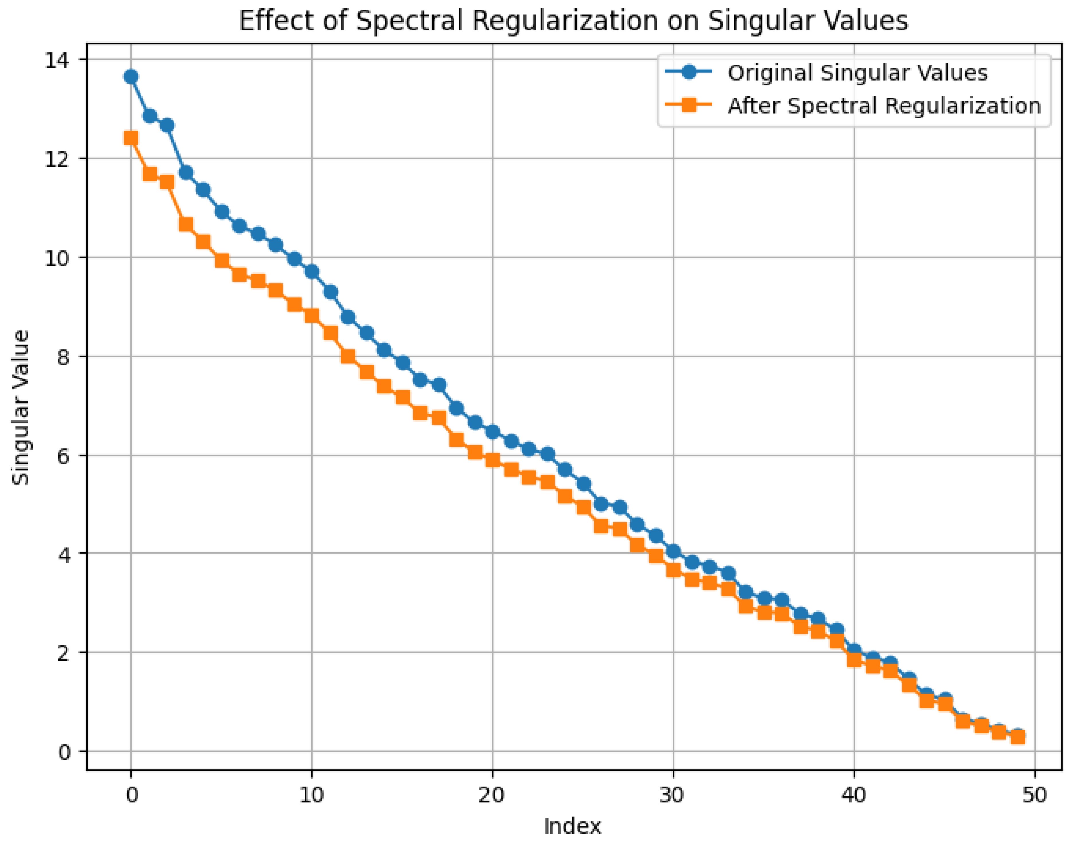
Figure 49.
Original Weight Matrix & After Spectral Regularization
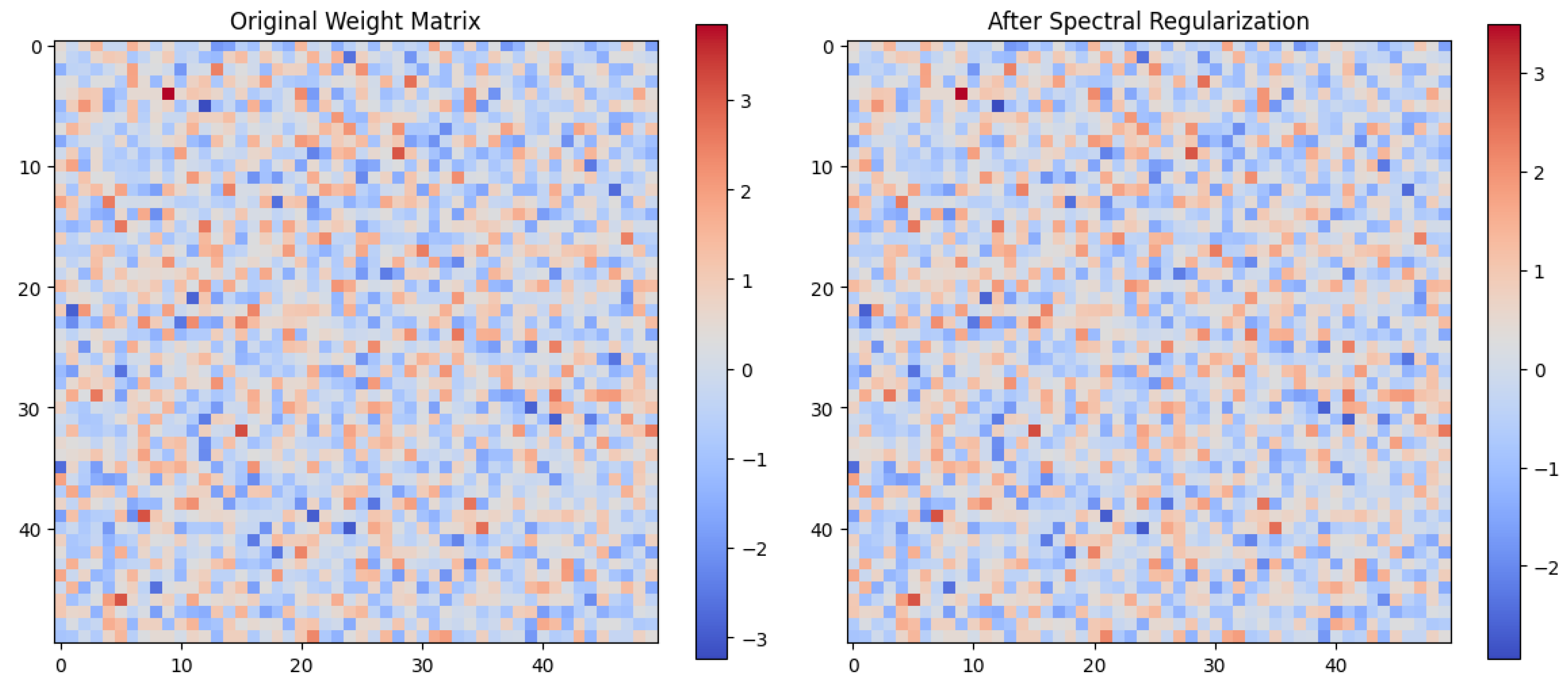
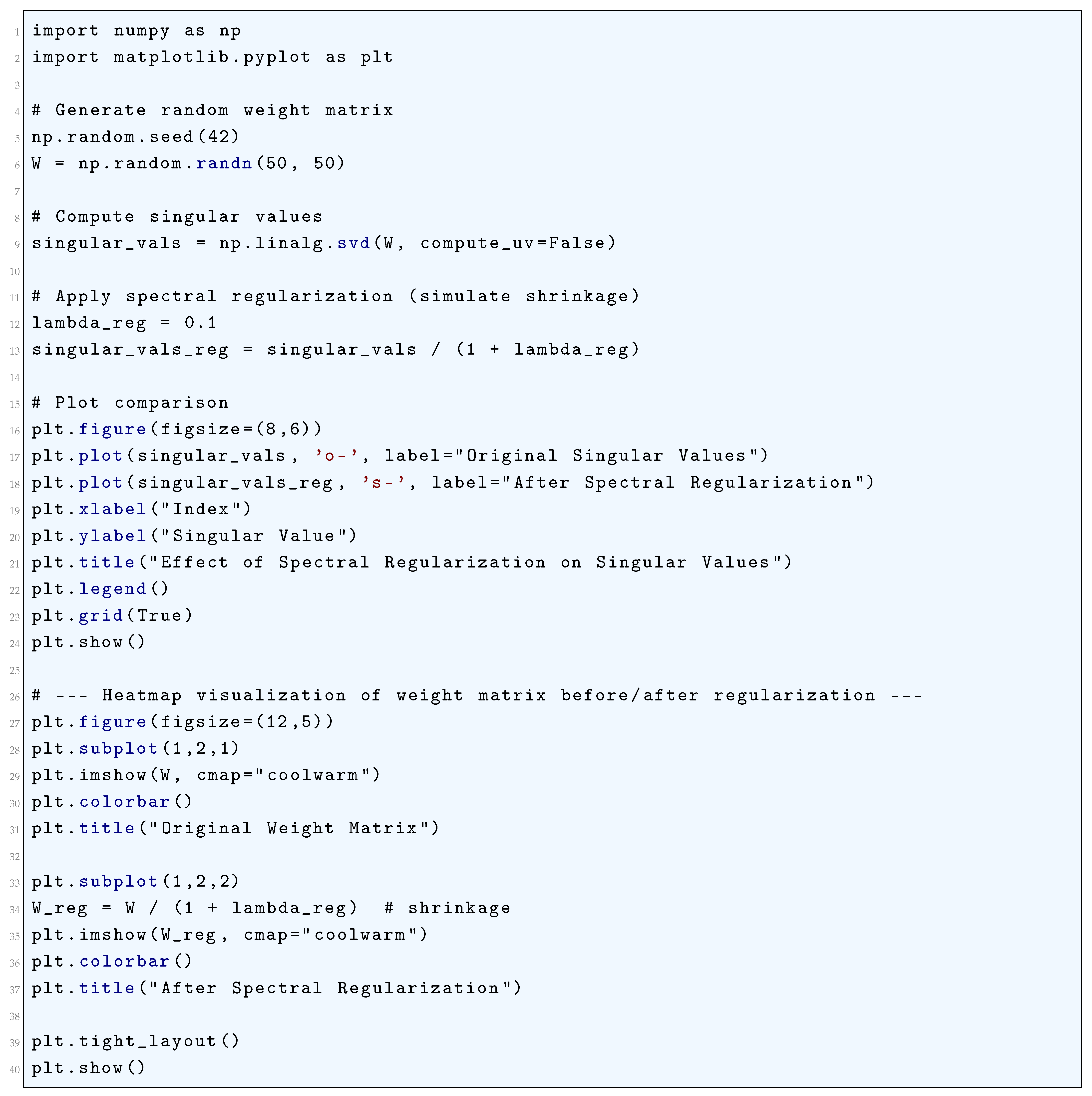
4.2.4. Python Code to Generate Figure 50 Illustrating Singular Value Spectrum of First Layer (MNIST)
The Python code below produces the Figure 50 illustrating Singular Value Spectrum of First Layer (MNIST).
Figure 50.
Singular Value Spectrum of First Layer (MNIST)
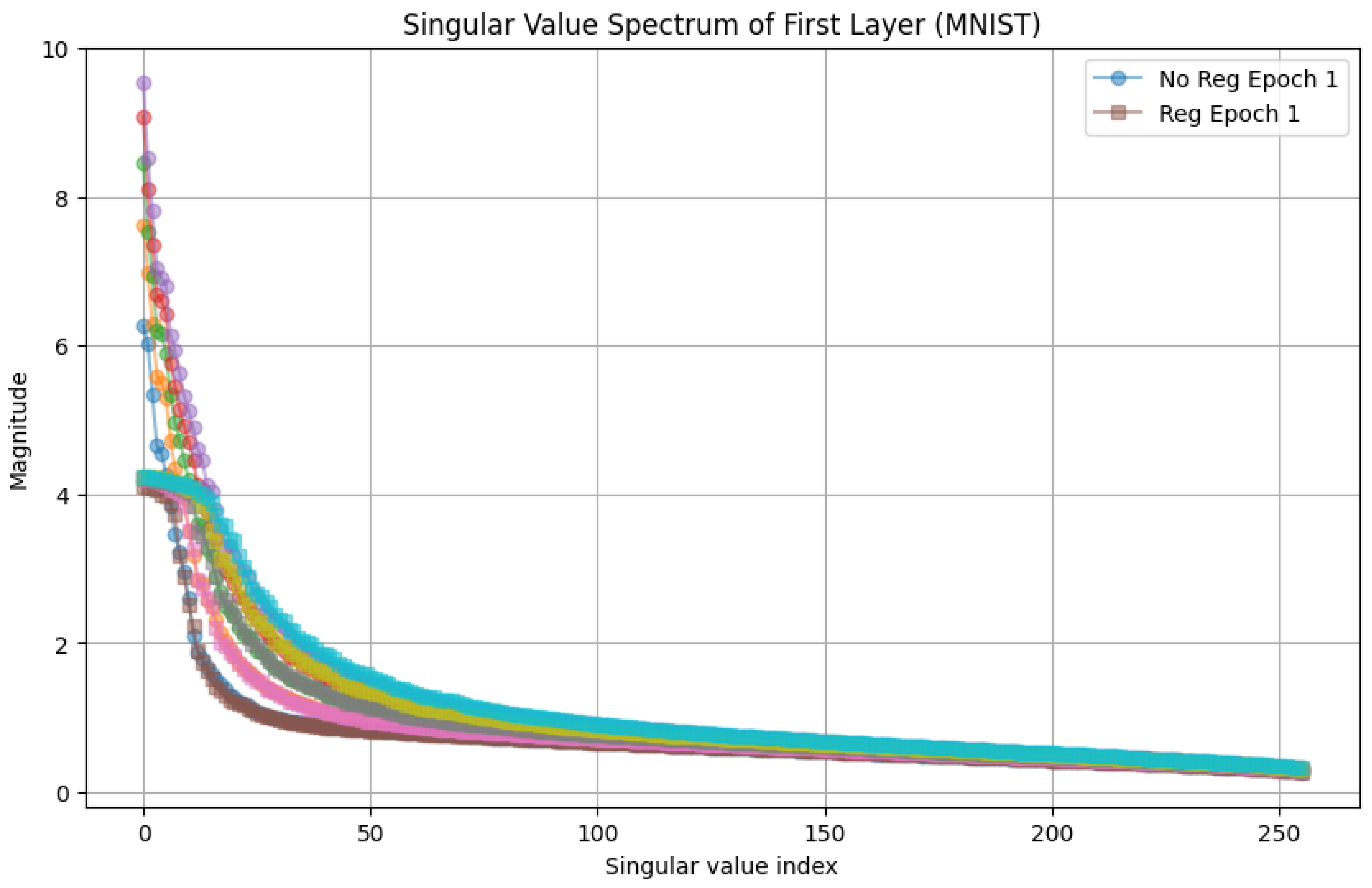
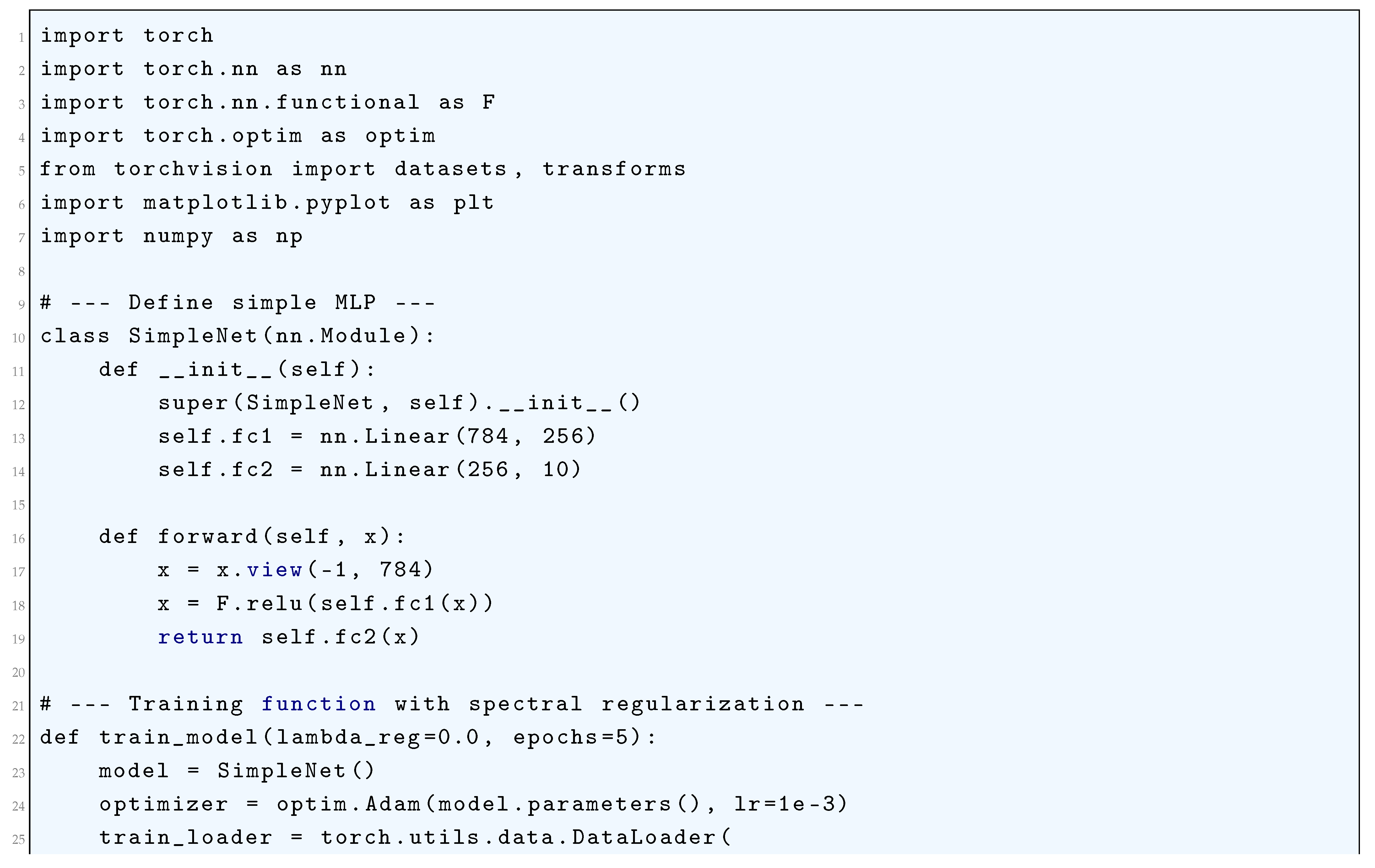
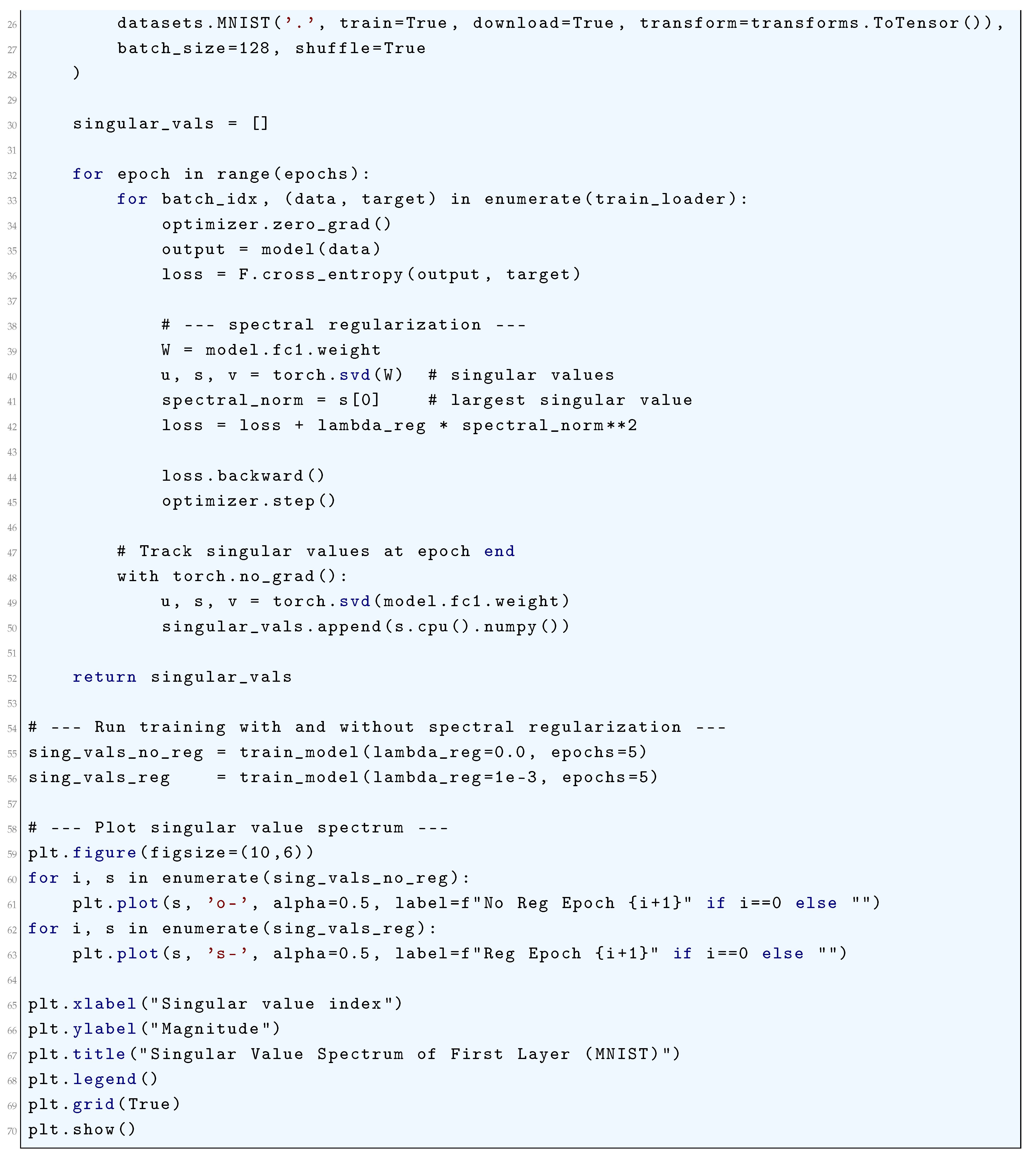
5. Game-Theoretic Formulations of Deep Neural Networks
The training of deep neural networks (DNNs) can be rigorously analyzed through game-theoretic frameworks, where optimization is interpreted as a competitive or cooperative interaction between different components of the model. In this setting, the learning process is modeled as a multi-player game, where each player corresponds to a subset of parameters (e.g., layers, neurons, or auxiliary networks), and their strategies are parameter updates that collectively influence the network’s performance. Let denote the parameters partitioned among K players. The objective is to minimize a global loss function , which induces a potential game where each player’s cost function aligns with the global loss. The Nash equilibrium of this game corresponds to a stationary point of , satisfying:
However, since exact equilibria are computationally intractable, training dynamics are often studied through online learning in games, where players iteratively adjust their strategies via gradient-based updates. For example, in generative adversarial networks (GANs), the generator and discriminator engage in a zero-sum game with value function:
where the generator seeks to minimize V while the discriminator maximizes it. The equilibrium corresponds to a saddle point satisfying:
The training dynamics of DNNs can also be formalized using differential game theory, where parameter updates follow continuous-time gradient flows. Consider a two-player game between feature extractors and classifiers in a deep network, where the state evolves according to the coupled ODEs:
The stability and convergence of such dynamics depend on the spectral properties of the game’s Jacobian matrix , defined as:
If has eigenvalues with negative real parts, the system converges to a stable equilibrium; otherwise, limit cycles or divergence may occur, as seen in GAN training. Furthermore, Stackelberg game formulations introduce hierarchical optimization, where one player (the leader, e.g., hyperparameters) commits to a strategy first, and the other (the follower, e.g., model parameters) responds optimally. This leads to bilevel optimization problems of the form:
These game-theoretic perspectives unify adversarial training, meta-learning, and multi-agent RL under a common framework, providing insights into convergence, robustness, and implicit regularization in deep learning.
5.1. Literature Review of Game-Theoretic Formulations of Deep Neural Networks
The game-theoretic formulations of deep neural networks have been explored extensively in recent literature, offering novel perspectives on optimization, adversarial robustness, and multi-agent interactions. One seminal contribution is the work by Goodfellow et al. (2014) [1472] on generative adversarial networks (GANs), which frames the training process as a two-player minimax game between a generator and a discriminator. This formulation has revolutionized unsupervised learning by enabling the generation of highly realistic data. The theoretical foundations of GANs have been further refined by Arjovsky et al. (2017) [1459], who introduced Wasserstein GANs to address convergence issues, providing a more stable training framework through the lens of optimal transport theory. Building on this, Gulrajani et al. (2017) [1473] proposed gradient penalty methods to enforce Lipschitz constraints, improving training stability. Another critical contribution comes from Shalev-Shwartz et al. (2012) [1495], who interpret supervised learning as a convex-concave game, establishing connections between empirical risk minimization and game-theoretic equilibria. This perspective has led to deeper insights into the generalization properties of neural networks, further explored by Hardt et al. (2016) [1475] through the lens of algorithmic stability.
The interplay between game theory and deep learning is also evident in adversarial robustness, where Madry et al. (2018) [1486] model adversarial attacks as a zero-sum game between a classifier and an adversary. Their work formalizes robust training as a min-max optimization problem, leading to the development of adversarially robust models. Similarly, Sinha et al. (2018) [1497] leverage distributionally robust optimization to frame adversarial training as a game against nature, providing probabilistic guarantees on model performance. These approaches highlight the utility of game-theoretic frameworks in addressing security challenges in deep learning, with additional insights from Raghunathan et al. (2018) [1492] on certified defenses and Zhang et al. (2019) [1502] on trade-offs between robustness and accuracy. Multi-agent reinforcement learning (MARL) is another domain where game theory plays a pivotal role. Littman’s (1994) [1483] formulation of Markov games extends single-agent reinforcement learning to competitive and cooperative settings, enabling the study of Nash equilibria in multi-agent systems. This has been expanded upon by Foerster et al. (2018) [1469], who introduce learning dynamics with opponent modeling, combining deep Q-learning with game-theoretic equilibria. Their work demonstrates how agents can adapt to others’ strategies in complex environments, a theme further developed by Lowe et al. (2017) [1484] with multi-agent actor-critic methods. Another notable contribution is by Lanctot et al. (2017) [1480], who propose the use of fictitious play and regret minimization in deep MARL, bridging the gap between classical game theory and modern deep learning techniques. Recent advances by Silver et al. (2017) [1496] in AlphaGo and OpenAI (2019) [1488] in multi-agent hide-and-seek showcase the practical success of these frameworks.
The optimization of neural networks has also been reinterpreted through game-theoretic lenses. For instance, Balduzzi et al. (2018) [1460] analyze gradient descent in deep learning as a dynamical system of interacting particles, drawing parallels to potential games. This perspective sheds light on the convergence behavior of neural networks, complemented by the work of Chizat & Bach (2018) [1462] on lazy training in wide networks. Meanwhile, Mertikopoulos et al. (2018) [1487] study the role of non-convexity in game-theoretic optimization, providing convergence guarantees for gradient-based methods in adversarial settings. Their work has implications for training GANs and other adversarial models, with additional theoretical grounding provided by Daskalakis et al. (2018) [1464] on the complexity of finding equilibria in non-convex games. Cooperative game theory has also found applications in explainability and feature attribution. Lundberg and Lee’s (2017) [1485] SHAP values, rooted in Shapley values from cooperative game theory, provide a principled framework for interpreting model predictions. This approach has been extended by Sundararajan et al. (2017) [1499] through integrated gradients, offering another game-theoretic perspective on feature importance. These methods have become standard tools for explainable AI, with further refinements by Janzing et al. (2020) [1477] on causal Shapley values and Frye et al. (2020) [1470] on contextual decomposition.
The intersection of game theory and deep learning continues to evolve, with recent work exploring mean-field games for large-scale multi-agent systems, as seen in the contributions of Carmona et al. (2019) [1461]. Their framework scales game-theoretic analysis to populations of agents, enabling applications in economics and robotics, with extensions by Perrin et al. (2020) [1491] on deep mean-field reinforcement learning. Another emerging direction is the use of auction theory in neural architecture search, where Liu et al. (2019) [1313] model the selection of network architectures as a combinatorial auction, optimizing resource allocation efficiently. These advancements underscore the breadth of game-theoretic applications in deep learning, from theoretical foundations to practical implementations, as seen in the work of Feng et al. (2020) [1467] on automated mechanism design. Further developments include the study of incentive alignment in federated learning, as explored by Li et al. (2020) [1482], who use mechanism design to ensure truthful participation among distributed agents. This line of work addresses challenges in collaborative learning environments, where strategic behavior must be accounted for, with additional insights from Kang et al. (2020) [1478] on reputation-based incentives. Additionally, the work of Letcher et al. (2019) [1481] on differentiable game theory provides tools for analyzing and optimizing the interactions of multiple loss functions in machine learning, offering a unified framework for multi-objective optimization, further refined by Schäfer & Anandkumar (2019) [1494] on competitive gradient descent.
The literature also delves into the role of information asymmetry in deep learning games, as exemplified by the work of Raghu et al. (2019) [1493] on signaling games in neural networks. Their analysis reveals how information bottlenecks emerge during training, influencing model behavior, with connections to the information bottleneck theory of Tishby et al. (2015) [1500]. Another significant contribution is by Perolat et al. (2022) [1489], who apply extensive-form games to hierarchical reinforcement learning, enabling sophisticated decision-making in structured environments, building on earlier work by Heinrich & Silver (2016) [1476] on fictitious self-play. Other notable contributions include the work of Czarnecki et al. (2020) [1463] on open-ended learning in games, which explores how agents can continuously adapt in dynamic environments, and the study of meta-learning in games by Al-Shedivat et al. (2018) [1458], which frames few-shot learning as a multi-agent interaction problem. The role of evolutionary dynamics in deep learning has been examined by Such et al. (2017) [1498], who apply population-based training to optimize hyperparameters, while Wang et al. (2019) [1501] explore the game-theoretic foundations of self-play in reinforcement learning.
Recent advances in differentiable economics by Dütting et al. (2019) [1466] and strategic classification by Hardt et al. (2016) [1475] further illustrate the growing synergy between game theory and deep learning. The work of Gemp et al. (2021) [1471] on resolving bargaining games with deep networks and the study of cooperative inverse reinforcement learning by Hadfield-Menell et al. (2016) [1474] highlight the potential for game-theoretic principles to guide AI alignment. Overall, the game-theoretic formulations of deep neural networks span a wide array of topics, from adversarial training and multi-agent systems to optimization and explainability. The contributions discussed here represent a fraction of the rich literature in this interdisciplinary field, which continues to grow as researchers uncover new connections between game theory and deep learning. Each of these works provides rigorous theoretical foundations, practical algorithms, or novel applications, collectively advancing our understanding of neural networks through the lens of game theory. The ongoing exploration of these ideas promises to yield further breakthroughs in the design, analysis, and deployment of intelligent systems.
5.2. Analysis of Game-Theoretic Formulations of Deep Neural Networks
Deep Neural Networks (DNNs) can be rigorously formulated within a game-theoretic framework by considering the interplay between competing objectives in optimization, adversarial robustness, and equilibrium strategies. The fundamental nature of DNNs involves a multi-agent optimization problem where various components interact within a high-dimensional function space.
Formally, a deep neural network is parameterized by a set of weights and seeks to optimize a loss function , where the training data is drawn from an unknown distribution. The optimization problem can be expressed as
A fundamental game-theoretic formulation of DNNs arises in adversarial training, where a deep network is trained to minimize an objective function while an adversary seeks to maximize it. This setting leads to a two-player zero-sum game where the adversary introduces perturbations such that the resulting optimization problem is
The equilibrium of this adversarial game corresponds to a minimax solution, satisfying the condition
If the loss function satisfies convexity in and concavity in , then the minimax theorem guarantees the existence of an equilibrium solution:
A notable game-theoretic application of DNNs is in Generative Adversarial Networks (GANs), where two neural networks, a generator and a discriminator , play a competitive game. The generator aims to produce realistic samples , while the discriminator seeks to distinguish between real and generated samples. The objective function for this adversarial game is
The Nash equilibrium condition for this game is given by
At equilibrium, the optimal generator satisfies
leading to a situation where the discriminator is unable to distinguish real from generated samples. If is parameterized by , then training the discriminator corresponds to solving
Given that neural networks can approximate arbitrary functions, their training can also be formulated in terms of multi-agent differential game theory.
Consider a dynamic system where the evolution of parameters follows
The Hamiltonian for this system is given by
where p is the costate variable and u represents control parameters. The Hamilton-Jacobi-Bellman equation characterizing optimal control in a reinforcement learning-based DNN training scenario is
Another approach to studying DNNs in a game-theoretic framework is through evolutionary game dynamics. Here, learning dynamics follow replicator equations given by
where represents the probability of selecting strategy i, is the fitness function for strategy i, and is the average fitness. In the context of neural networks, the replicator equation governs weight updates as follows:
This provides a mechanism for gradient-based optimization that incorporates selection and mutation principles.
Another critical formulation involves Nash equilibria in non-cooperative learning settings, such as federated learning, where multiple learners optimize separate but interdependent loss functions. The Nash equilibrium conditions require that
where denotes the set of parameters for all players except i. A Nash equilibrium is attained when
Under convexity assumptions, Nash learning dynamics can be characterized by a gradient projection algorithm:
Beyond Nash equilibria, deep neural networks can also be analyzed through variational inequalities, which generalize equilibrium concepts. Given a function , the variational inequality problem seeks such that
For adversarial training, the corresponding variational inequality formulation is
where denotes the optimal adversarial perturbation satisfying
This variational inequality provides a principled characterization of adversarial robustness in deep networks. The application of game-theoretic formulations to deep learning thus allows for a mathematically rigorous understanding of optimization, equilibrium conditions, and strategic interactions among network components.
5.2.1. Python Code to Generate Figure 51, Figure 52, and Figure 53 Illustrating Game-Theoretic Formulations of Deep Neural Networks
The Python code below produces the Figure 51, Figure 52, and Figure 53 illustrating Game-theoretic formulations of Deep Neural Networks.
Figure 51.
Min-Max Game Formulation (Adversarial Training)
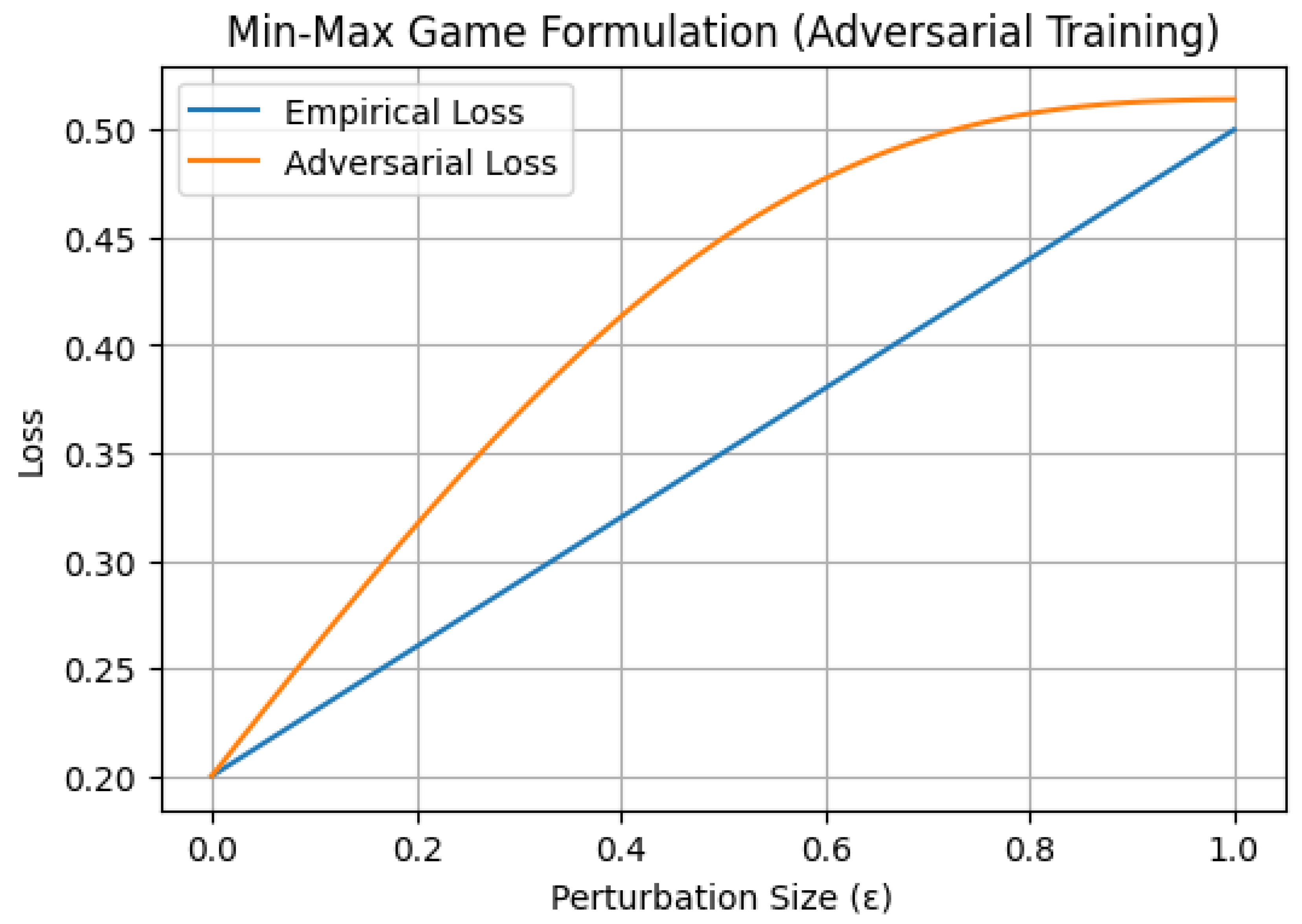
Figure 52.
Regularization as Game Formulation
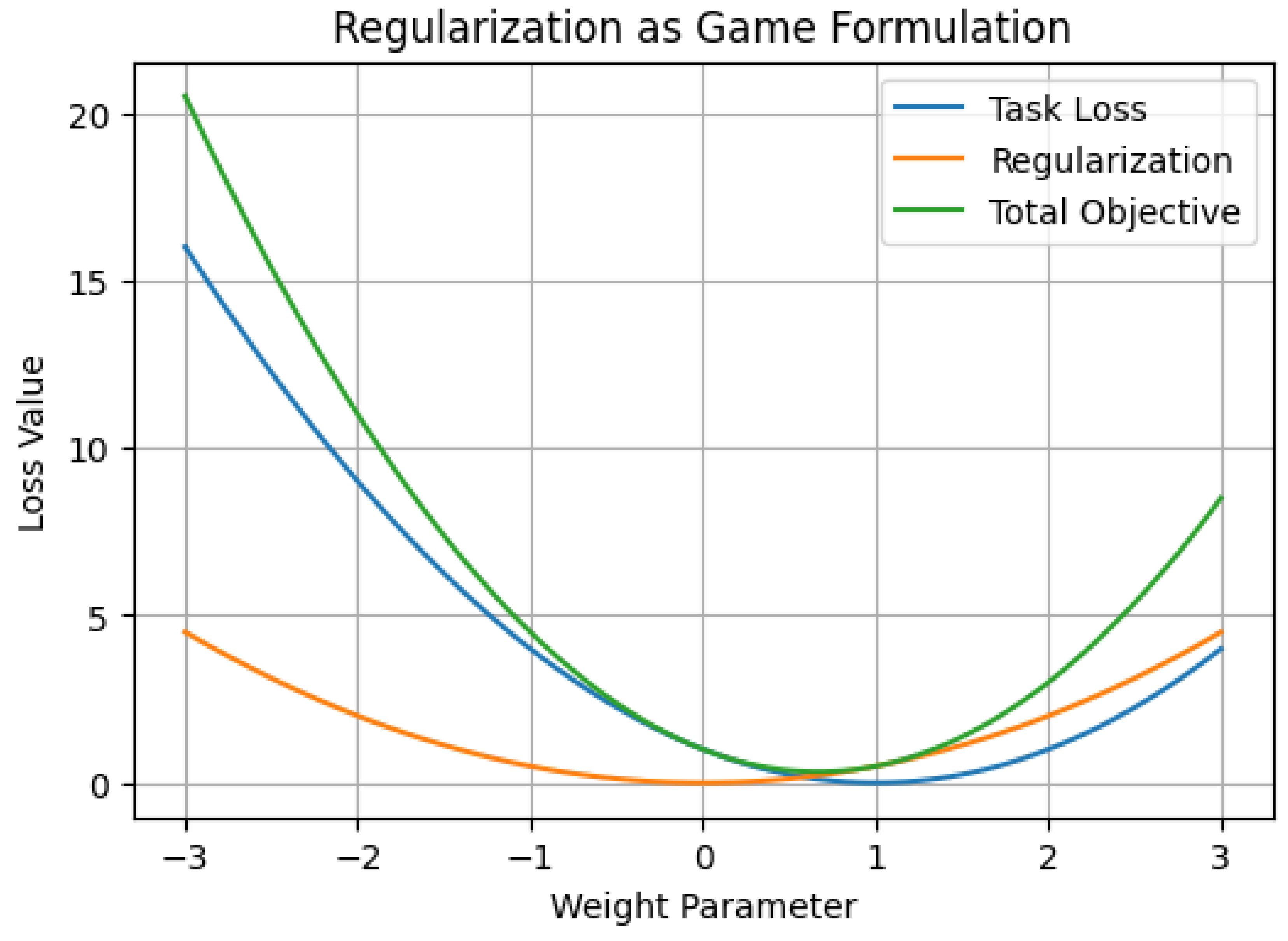
Figure 53.
Multi-Agent Game: Layers as Players
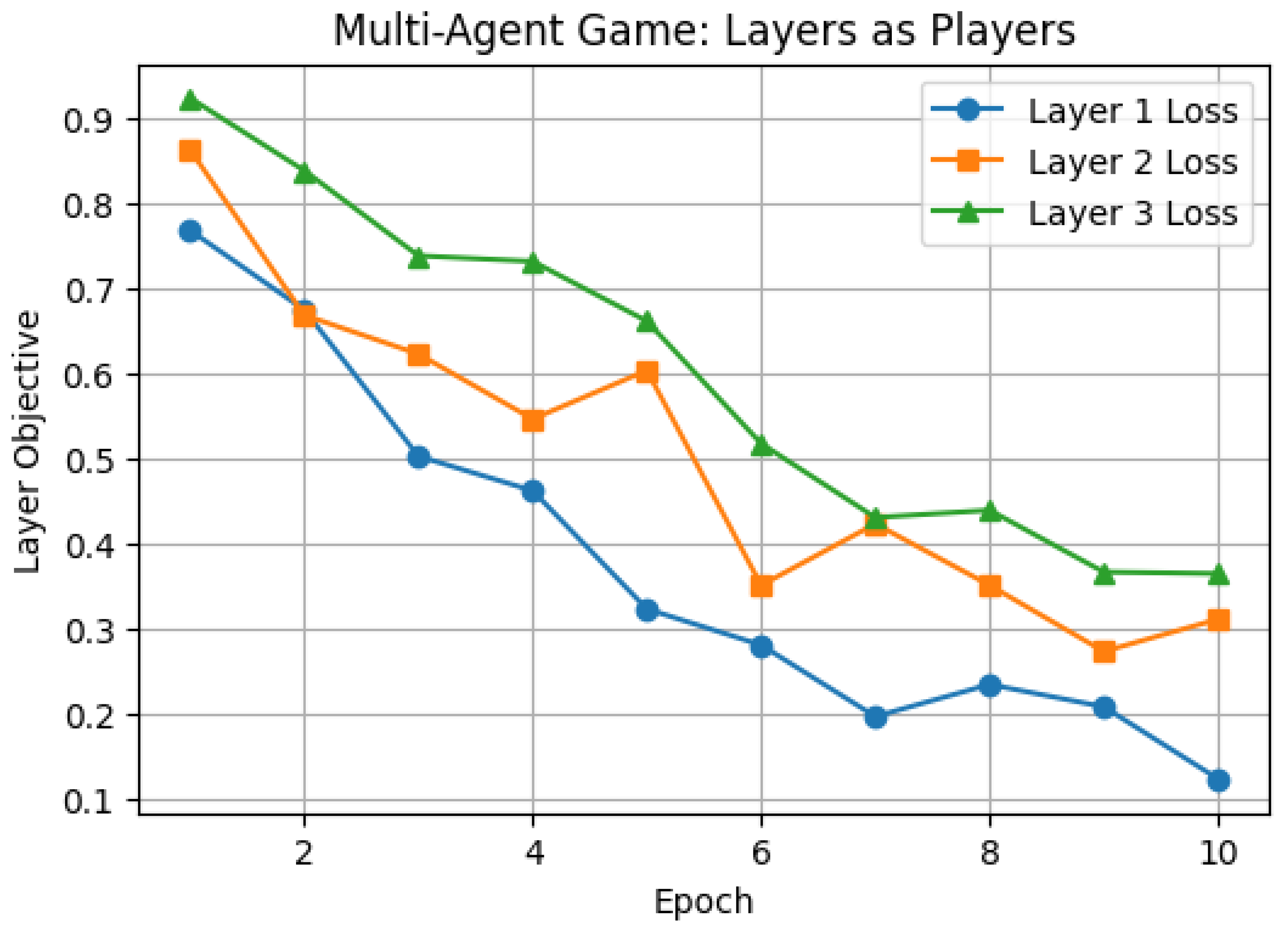
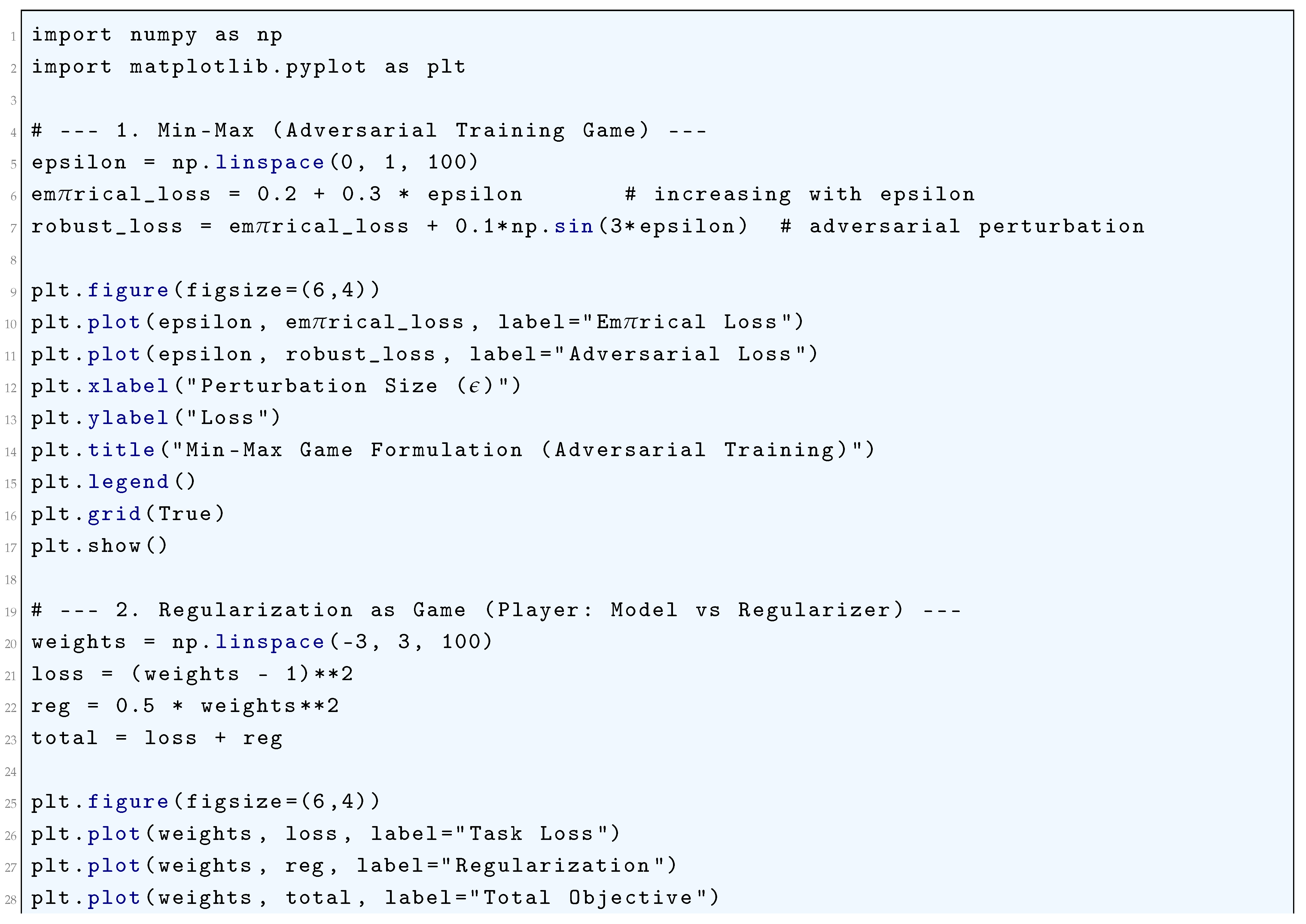
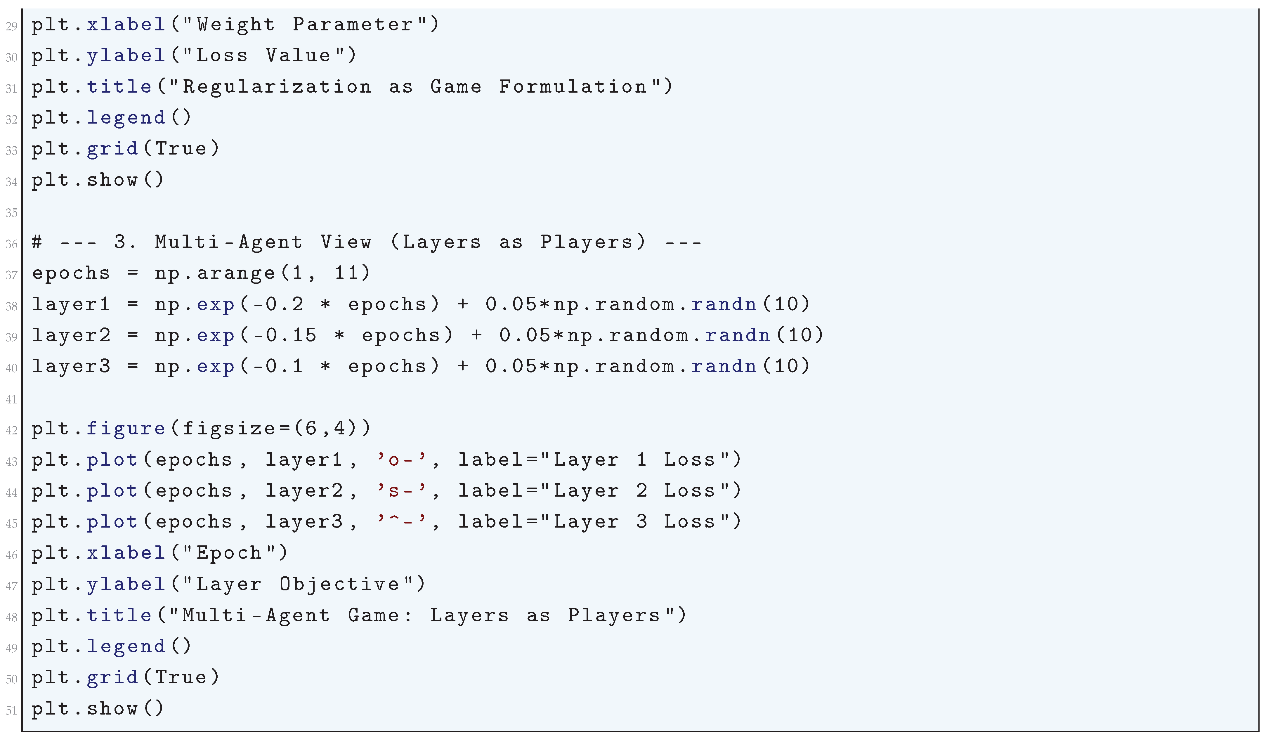
5.2.2. Min-Max (Saddle) Dynamics:
The function that serves as a canonical, analytically tractable model for studying the min-max saddle point dynamics that is central to the training of Generative Adversarial Networks (GANs) and other adversarial learning formulations within deep learning is
In this game-theoretic framework, the two players are the generator and the discriminator, whose parameters are abstracted here by the variables y and x, respectively.
The discriminator’s objective is to maximize the payoff function , while the generator’s objective is to minimize it. This defines a zero-sum game with the value function
and the overall goal is to find a Nash equilibrium, which is a point satisfying the saddle point condition
for all x and y in a local neighborhood.
The dynamics of the training process are typically modeled by simultaneous or alternating gradient descent-ascent. The vector field governing these dynamics is given by the gradients of the objective with respect to each player’s variable. For the bilinear objective , these gradients are
The simultaneous gradient descent-ascent update rule with learning rate is
and
This system of equations is linear and can be written in matrix form as
and
The eigenvalues of this update matrix are , which have magnitude . This implies that the dynamics are unstable and will diverge for any , causing the players’ parameters to orbit the equilibrium point on a trajectory of exponentially increasing radius. This simple model thus captures a fundamental pathology in adversarial training: the vector field
is non-conservative and has a non-zero rotational component, preventing convergence under naive gradient-based methods.
The divergence of this simple dynamic motivates the need for more sophisticated optimization algorithms in practical deep neural network training. The bilinear term is often a component of a larger loss landscape, and its presence induces rotational forces that can destabilize training. Algorithms such as Optimistic Mirror Descent (OMD) and the closely related Extra Gradient (EG) method are designed to counteract this instability. For example, the Optimistic Mirror Descent update for this problem is given by
and
The spectral analysis of this system reveals that it can converge for a sufficiently small learning rate , unlike the divergent simultaneous gradient method. The core mathematical insight is that the stability of the learning dynamics depends critically on the structure of the game’s Jacobian,
For the bilinear game, this Jacobian is a skew-symmetric matrix, and convergence guarantees for algorithms like OMD and EG are derived by showing that their update operators can mitigate the rotational effects encoded by this skew-symmetric component, thereby allowing the dynamics to spiral inward towards the saddle point rather than outward to infinity.
5.2.3. Potential/Cooperative Game (Gradient Descent on Shared Phi)
In the game-theoretic analysis of deep neural network training, a potential or cooperative game represents a foundational scenario where the interests of all parameter blocks are perfectly aligned. This framework is defined by the existence of a global, differentiable potential function , where represents the concatenated parameters of all N players or network components. The individual loss function for each player i is precisely this shared potential
for all i. Consequently, the game is one of pure cooperation, as all players share the identical objective of minimizing . The dynamics are governed by the simultaneous gradient, which is simply the full gradient of the potential function:
The learning process in this setting is equivalent to gradient descent on the shared objective . The continuous-time dynamics are described by the ordinary differential equation
where is the learning rate. The discrete-time update with a fixed learning rate is given by
A first-order Taylor expansion reveals the change in the potential function:
where
is the Hessian matrix of the potential. For sufficiently small such that
in the positive definite sense, the term linear in dominates, guaranteeing a decrease in the potential:
The game-theoretic properties are analyzed through the lens of the game Jacobian, , which is defined as the matrix of second-order derivatives of the individual losses.
For a potential game, this Jacobian is given by
This implies that is equivalent to the Hessian of the potential function, . A critical mathematical consequence is that the Jacobian of a potential game is symmetric
This symmetry is the defining characteristic of a potential game and ensures that the dynamics are a gradient flow. The eigenvalues of are all real, and their signs determine the stability of critical points. A point is a Nash equilibrium if
and it is a locally stable equilibrium under gradient descent if
meaning all eigenvalues of the Hessian are positive.
The convergence analysis leverages Lyapunov stability theory. The potential function itself serves as a Lyapunov function for the gradient dynamics. Its time derivative along the trajectories of the continuous-time system is
This quantity is strictly negative everywhere except at critical points where , confirming the global stability of the dynamics. In the discrete-time setting, under the assumption that is L-smooth, meaning
which implies
one can derive a quantitative convergence rate. Applying this at
yields
For a learning rate , this guarantees a monotonic decrease in the potential. After T iterations, the best iterate satisfies
where is the minimal value, proving convergence to a stationary point at a rate of . This mathematically rigorous framework provides the foundational guarantees for standard, non-adversarial deep learning, where the optimization landscape, despite its non-convexity, is traversed by a single, cohesive gradient flow.
5.2.4. Replicator Dynamics (Rock-Paper-Scissors) — Cyclic Behavior
The Replicator Dynamics equation, a cornerstone of evolutionary game theory, provides a continuous-time model for the evolution of strategy frequencies within a population. For a game with n pure strategies and a payoff matrix A, where denotes the payoff for strategy i against strategy j, the dynamics are defined for a population state , the -dimensional simplex where and . The rate of change of the frequency is given by
The term
is the expected payoff for strategy i, and
is the average payoff across the entire population. This equation dictates that strategies yielding above-average payoff proliferate, while those with below-average payoff diminish.
The Rock-Paper-Scissors (RPS) game is the canonical example of a zero-sum, non-transitive game that induces cyclic behavior under these dynamics. Its payoff matrix for the row player is given by
The average payoff in the population for this antisymmetric matrix () is always zero, , simplifying the replicator dynamics to . Writing these equations explicitly for the three strategies (Rock R, Paper P, Scissors S) yields the system:
The dynamics of this system conserve a specific quantity, which can be found by analyzing the time derivative of the logarithm of the product . Specifically,
This implies that the function
is a constant of motion, and consequently, the quantity
remains constant along any trajectory of the dynamics. The orbits of the system are closed curves defined by the level sets of K, resulting in perpetual, neutrally stable cycles around the interior Nash equilibrium .
This cyclic behavior is not merely a pathological example but a fundamental model for understanding non-convergent dynamics in multi-agent learning systems, including certain regimes in the training of deep neural networks, particularly Generative Adversarial Networks (GANs). The vector field defines a flow on the simplex. The Jacobian of this vector field at the interior equilibrium is
This matrix is skew-symmetric, , and its eigenvalues are . The purely imaginary conjugate pair confirm the presence of a center manifold, leading to oscillatory behavior. The connection to deep learning is established by noting that the simultaneous gradient descent-ascent dynamics on a bilinear loss function
which abstracts the interaction between two neural networks like a generator and a discriminator, yield a structurally similar vector field
For an antisymmetric A, this becomes
whose second-order form
describes a multi-dimensional harmonic oscillator. This mathematical equivalence demonstrates how the replicator dynamics’ inherent cycles manifest as rotational forces and training instability in adversarial neural network training, preventing convergence to a stationary Nash equilibrium.
5.2.5. Python Code to Generate Figure 54, Figure 55 and Figure 56 Illustrating Min-Max (Saddle) Dynamics, Potential/Cooperative Game (Gradient Descent on Shared Phi), and Replicator Dynamics (Rock-Paper-Scissors) — Cyclic Behavior
The Python code below produces the Figure 54, Figure 55 and Figure 56 illustrating Min-Max (Saddle) dynamics, Potential/Cooperative game (gradient descent on shared Phi), and Replicator dynamics (Rock-Paper-Scissors) — cyclic behavior.
Figure 54.
Min-Max (Saddle) dynamics:
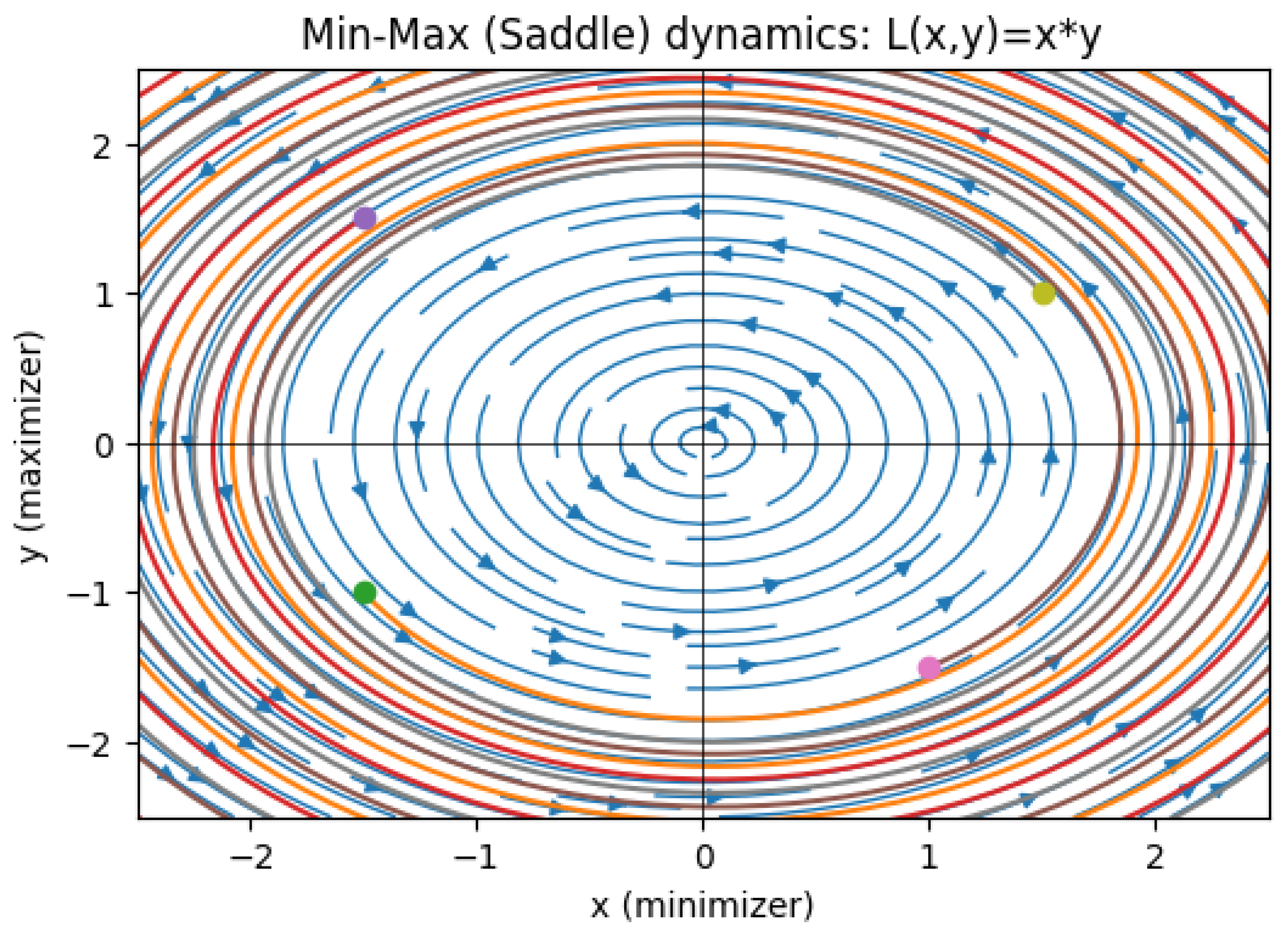
Figure 55.
Potential / Cooperative game (gradient descent on shared Phi)
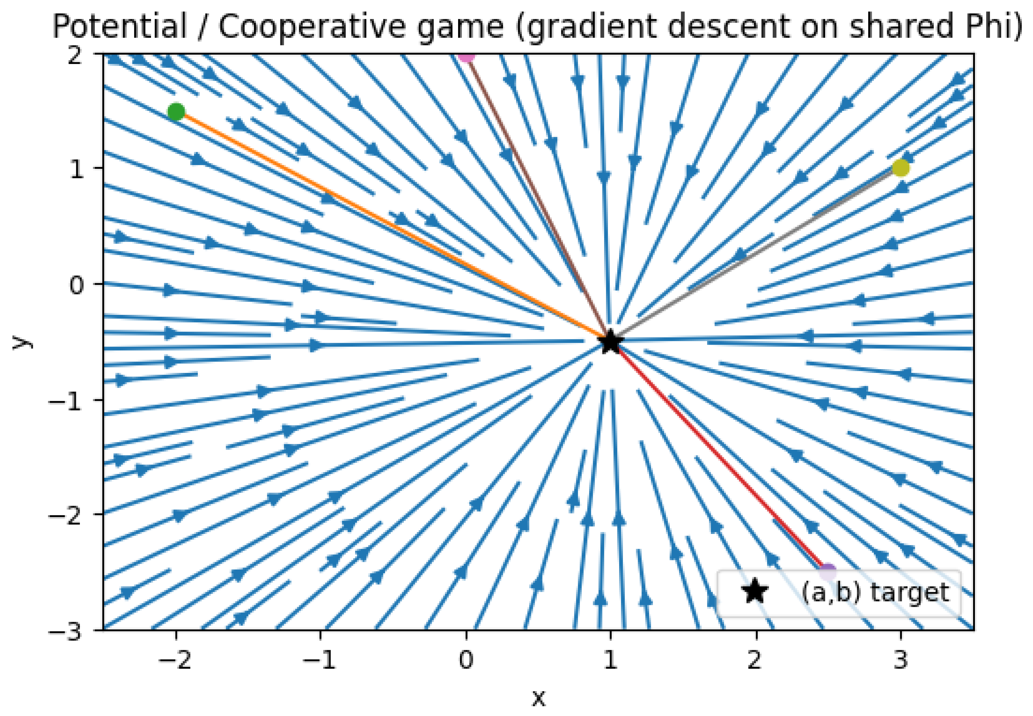
Figure 56.
Replicator dynamics (Rock-Paper-Scissors) — cyclic behavior
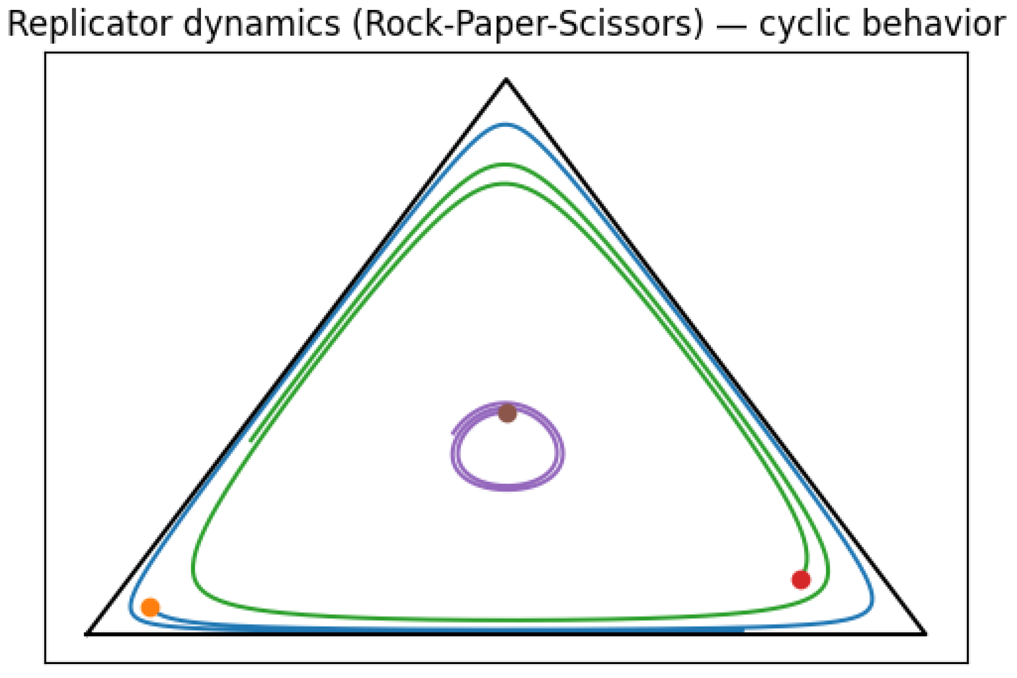
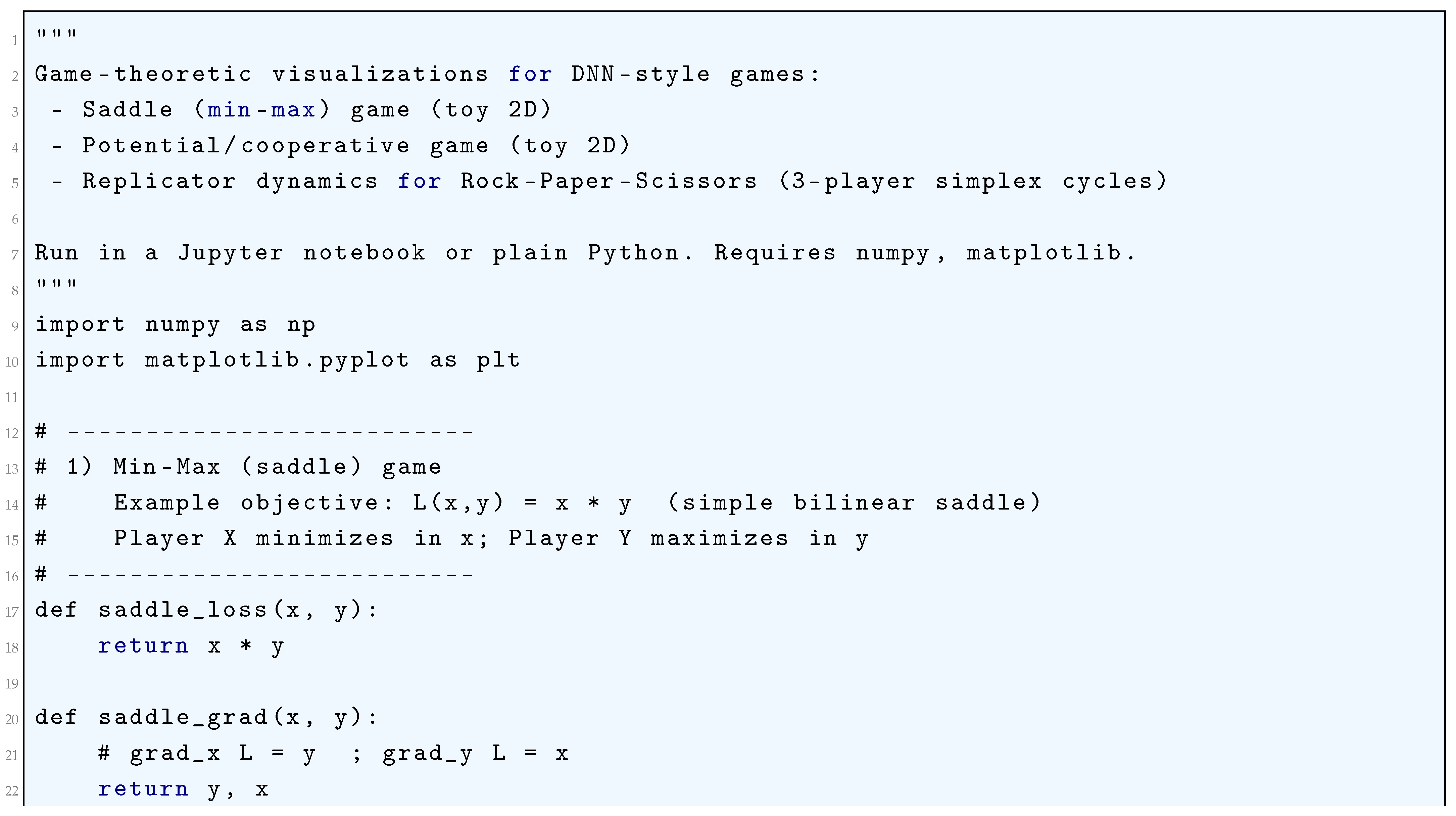
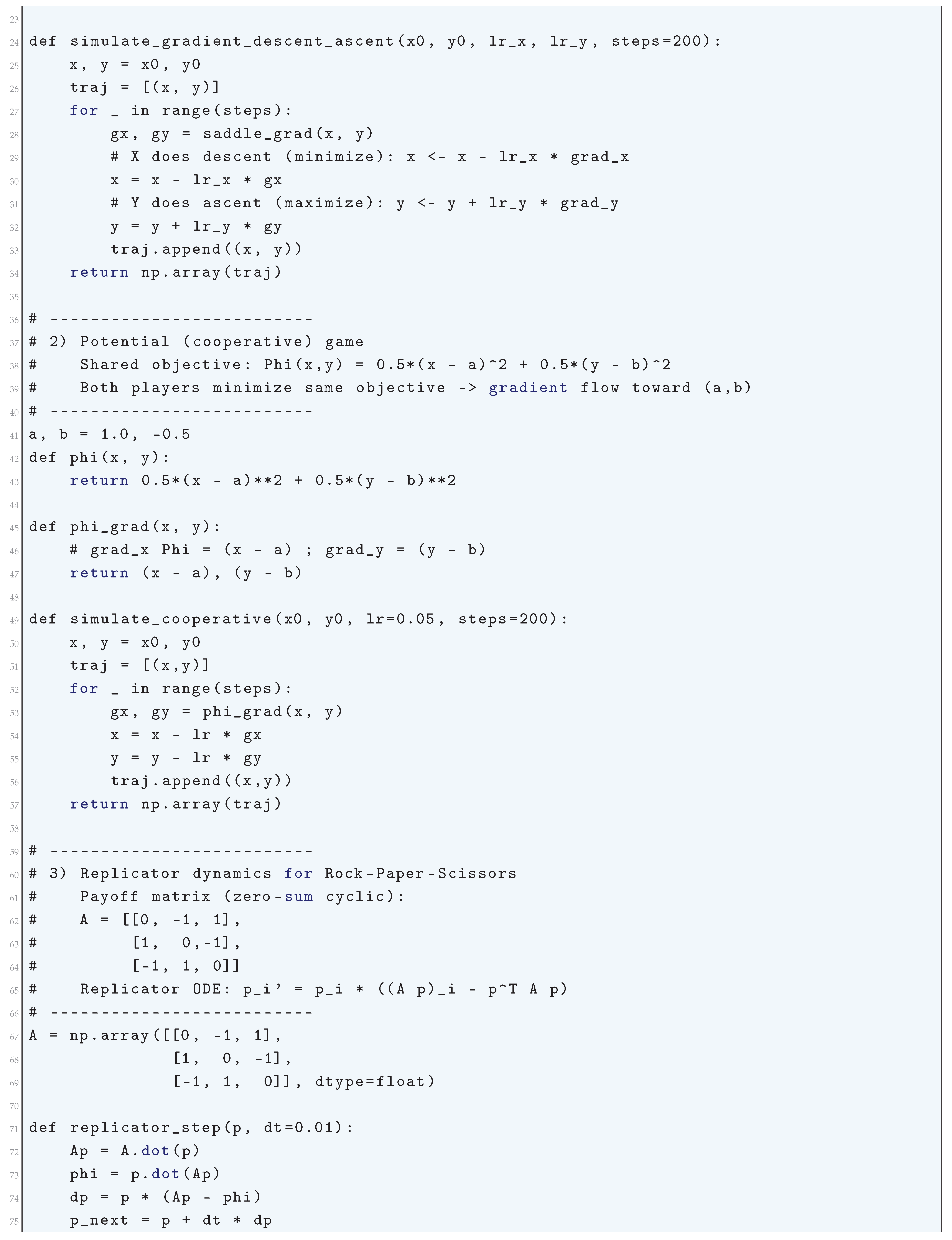
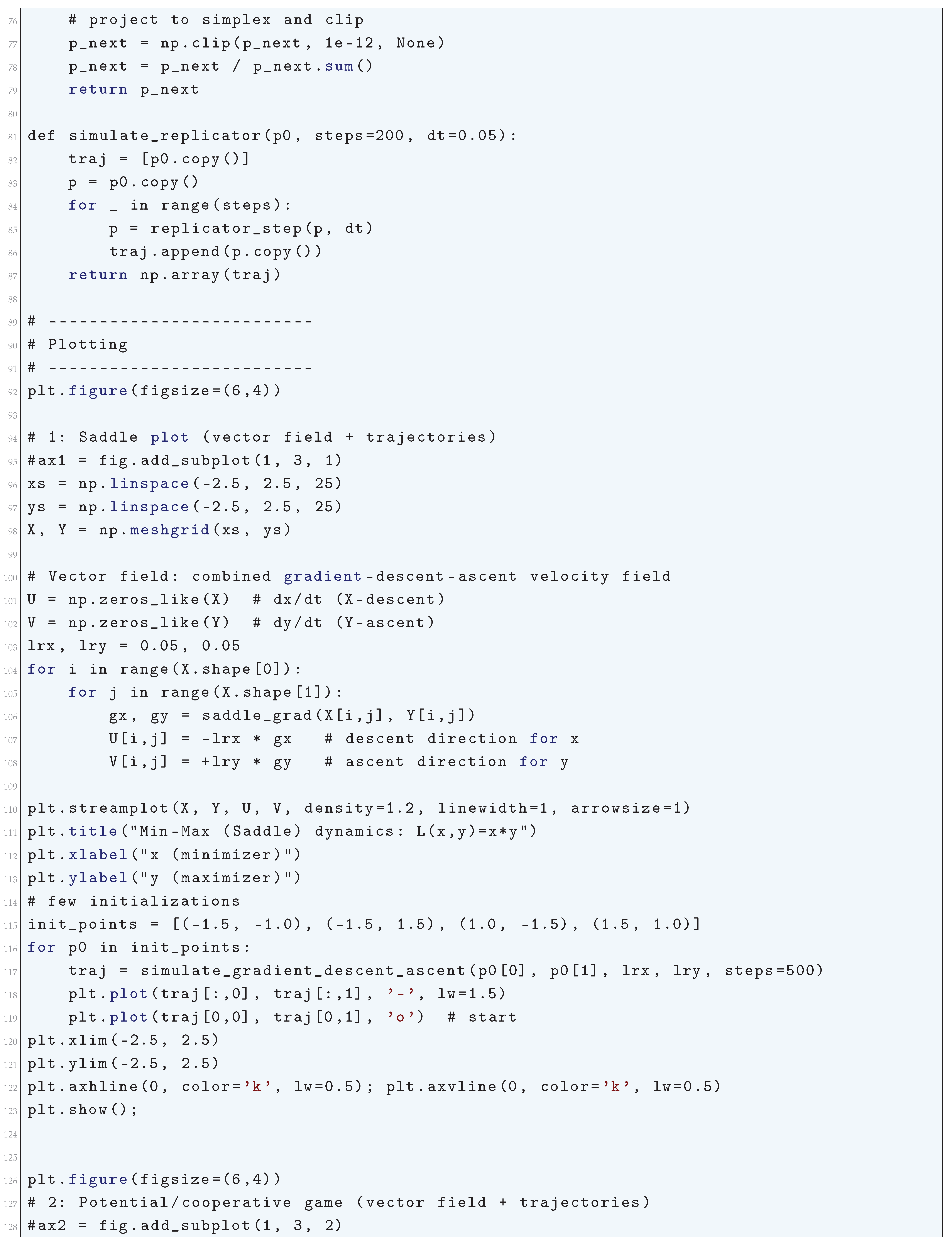
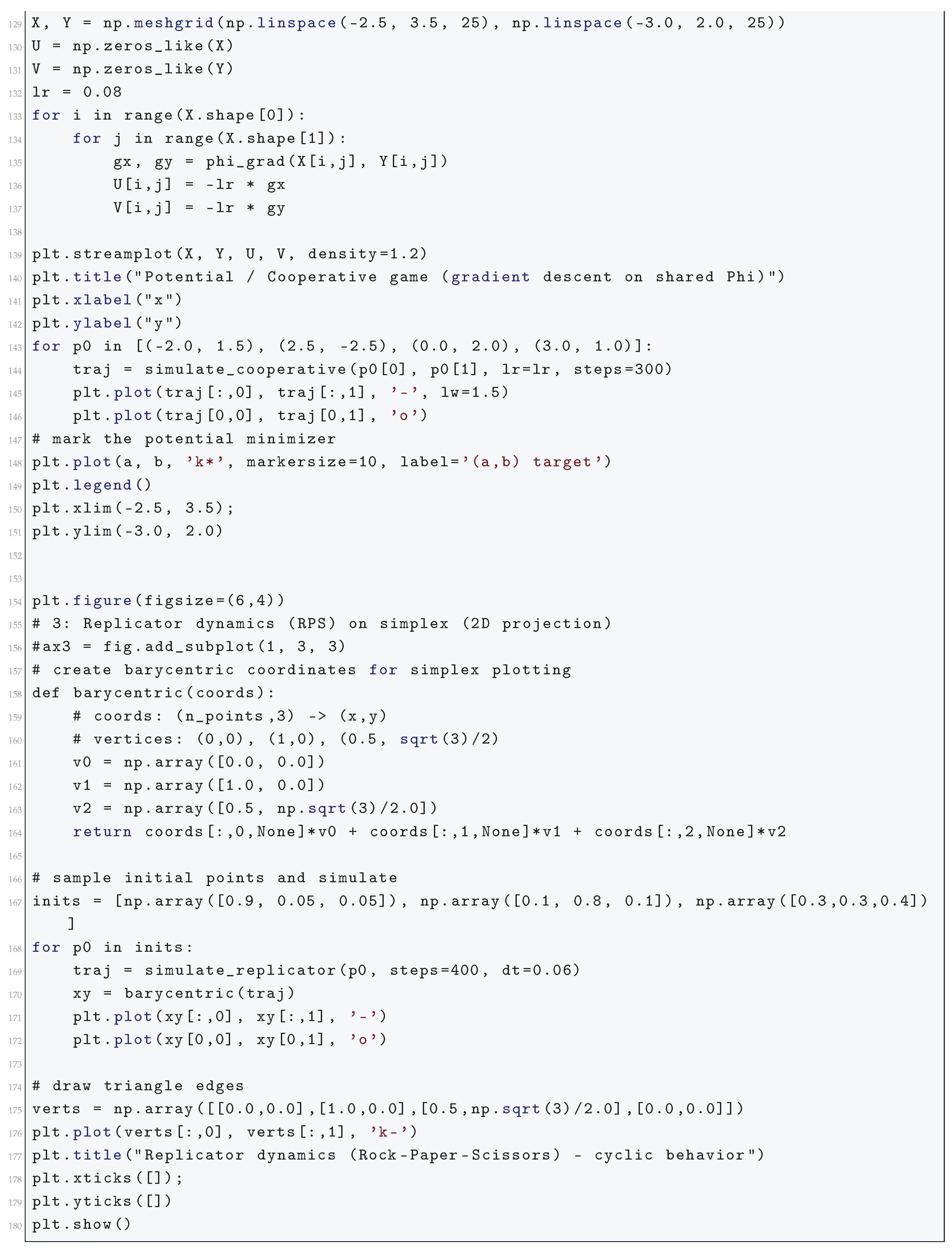
5.3. Game-Theoretic Formulations of Deep Neural Networks (DNNs) Through Evolutionary Game Dynamics
Deep neural networks (DNNs) can be formulated within the framework of evolutionary game dynamics, where the optimization of network parameters is recast as a competitive evolutionary process in which different parameter configurations act as strategies that undergo selection, mutation, and adaptation over time. This perspective allows a rigorous characterization of learning dynamics through replicator equations, Nash equilibria, and mutation-selection balance, thereby linking deep learning to fundamental principles in game theory and statistical physics. Given a neural network parameterized by , where is the space of all possible weight configurations, the performance of the network is quantified by a fitness function , which is typically defined as the negative of the empirical loss function . This loss function can be expressed as an expectation over a given dataset D,
where ℓ represents the pointwise loss function, such as the squared error loss or cross-entropy loss. The fitness of a given parameter configuration is then defined as
which ensures that lower loss corresponds to higher fitness. The evolutionary distribution of network parameters, denoted by , follows an evolutionary replicator-mutator equation,
where is the mean fitness across all parameter configurations,
The first term in the equation represents selection dynamics, where parameter configurations with higher fitness proliferate, while the second term models mutations, accounting for stochastic noise in learning updates. The steady-state solution to this equation corresponds to an evolutionarily stable distribution , which satisfies
for any small perturbation from . The learning process in deep networks can thus be viewed as an evolutionary competition in which weight distributions evolve toward stable equilibria or limit cycles.
The standard stochastic gradient descent (SGD) update rule, given by
can be reinterpreted as a mean-field approximation of the replicator equation with stochastic diffusion,
where represents a stochastic perturbation modeling noise in the gradient updates. In the limit of infinitesimally small learning rate , the SGD update can be seen as an Ornstein-Uhlenbeck process,
where denotes a Wiener process. The equilibrium distribution of network parameters is then governed by the Fokker-Planck equation,
This equation describes the evolution of the probability density of weight configurations under a combination of gradient descent and stochastic exploration, which can be interpreted as a mutation-selection process in an evolutionary game.
The steady-state solution corresponds to a Boltzmann-Gibbs distribution,
where acts as an inverse temperature parameter, and Z is the partition function ensuring normalization. This establishes a direct connection between deep learning optimization and principles of statistical mechanics, whereby learning dynamics resemble an energy minimization process subject to thermal noise. In the case of generative adversarial networks (GANs), the evolutionary perspective is particularly insightful. A GAN consists of a generator G and a discriminator D, which play a two-player zero-sum game governed by the minimax objective,
The training dynamics of GANs exhibit co-evolutionary behavior, which can be captured by the coupled replicator equations,
Unlike standard deep learning, GAN training often fails to converge to an equilibrium due to cycling behavior.
This phenomenon can be analyzed through Hamiltonian game dynamics,
These equations describe a conservative dynamical system, where learning trajectories follow closed orbits rather than converging to fixed points. This behavior is characteristic of zero-sum games and is mathematically analogous to the Red Queen effect in evolutionary biology, where competing species continually adapt without achieving a stable equilibrium.
5.3.1. Python Code to Generate Figure 57, Figure 58 and Figure 59 Illustrating Game-Theoretic Formulations of Deep Neural Networks (DNNs) Through Evolutionary Game Dynamics
The Python code below produces the Figure 57, Figure 58 and Figure 59 illustrating Game-theoretic formulations of deep neural networks (DNNs) through Evolutionary Game Dynamics.
Figure 57.
Replicator Dynamics as Gradient Descent
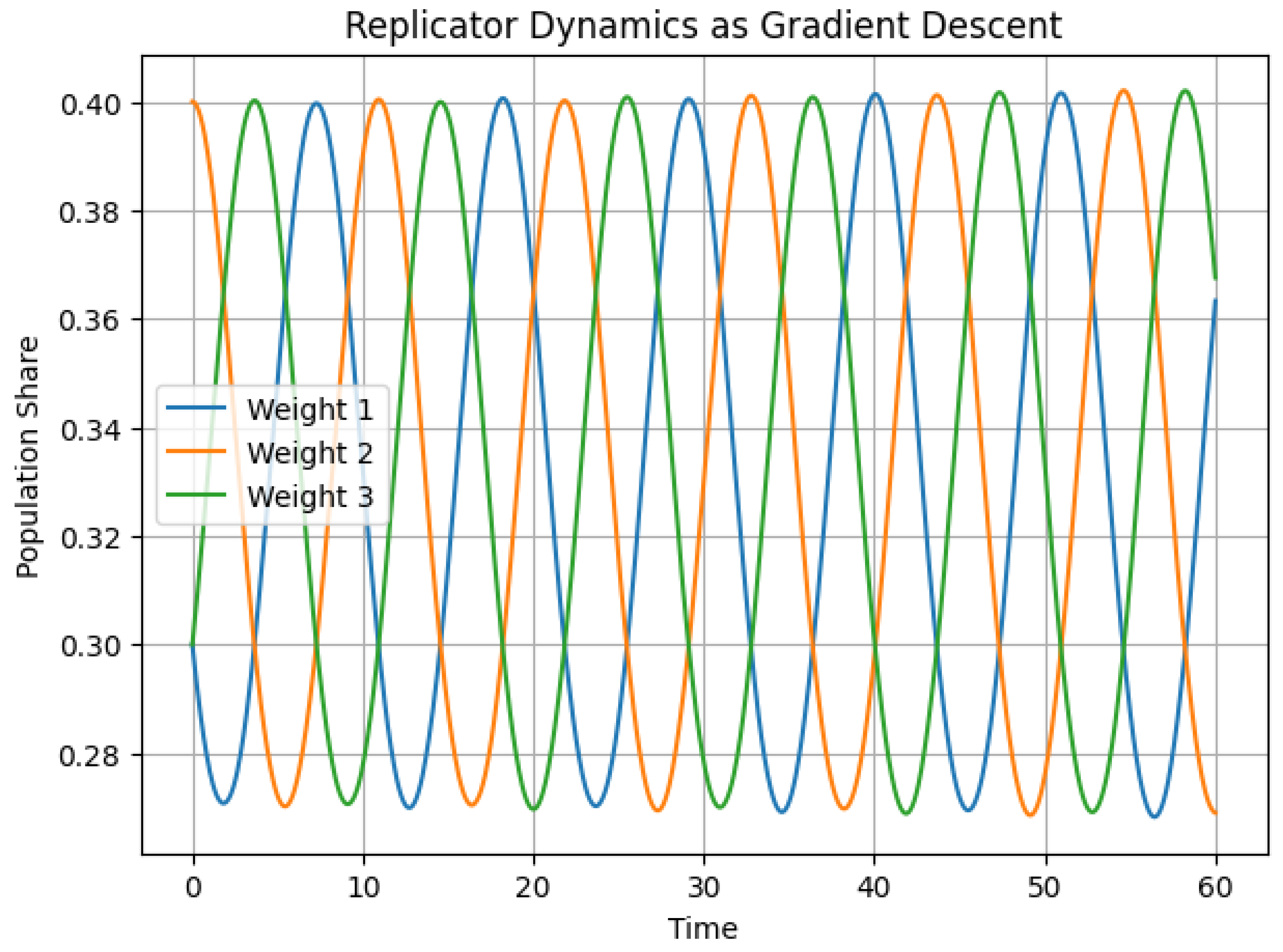
Figure 58.
Min-Max Dynamics (Adversarial Training)
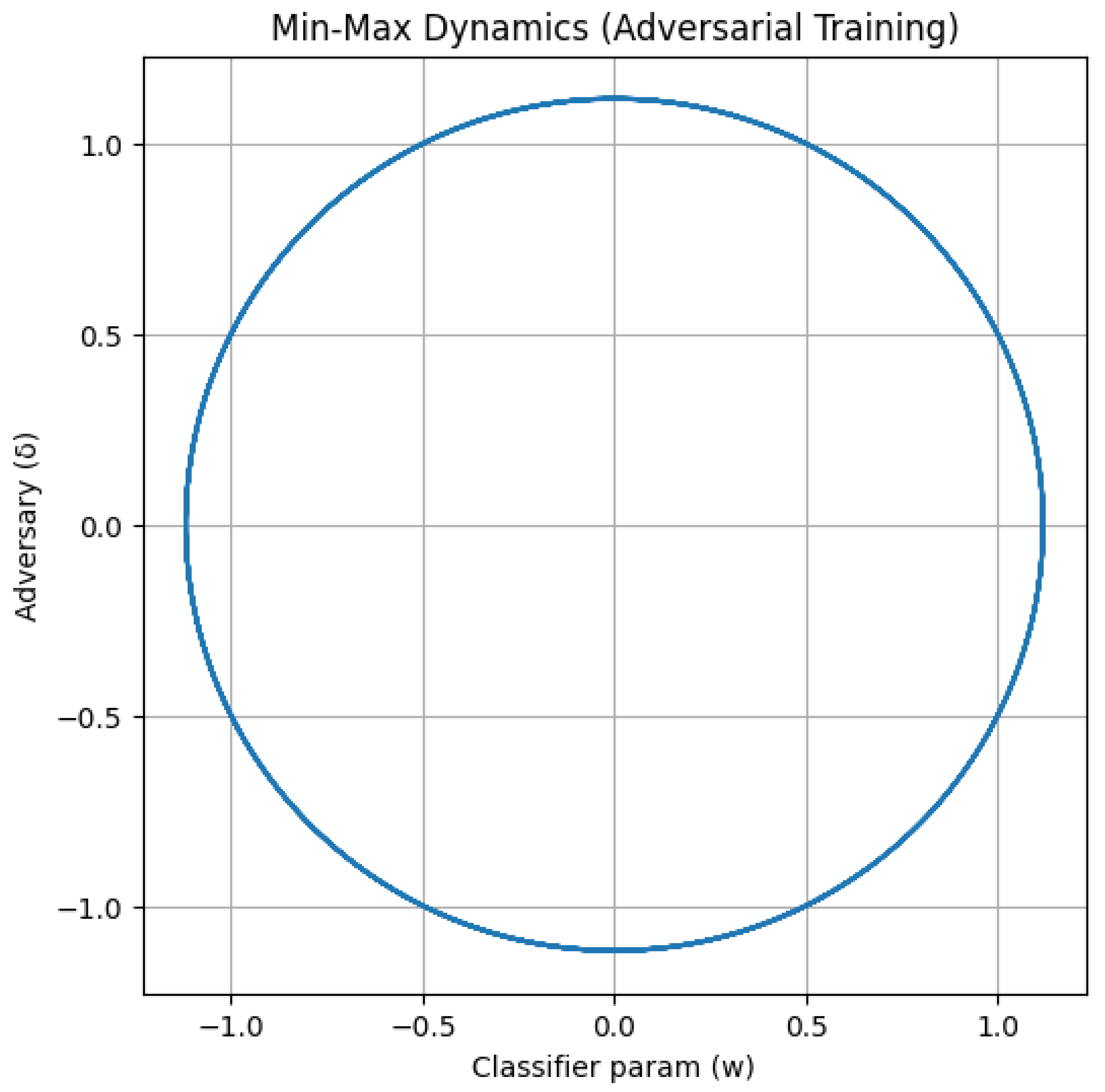
Figure 59.
Cooperative Game (Shared Potential)
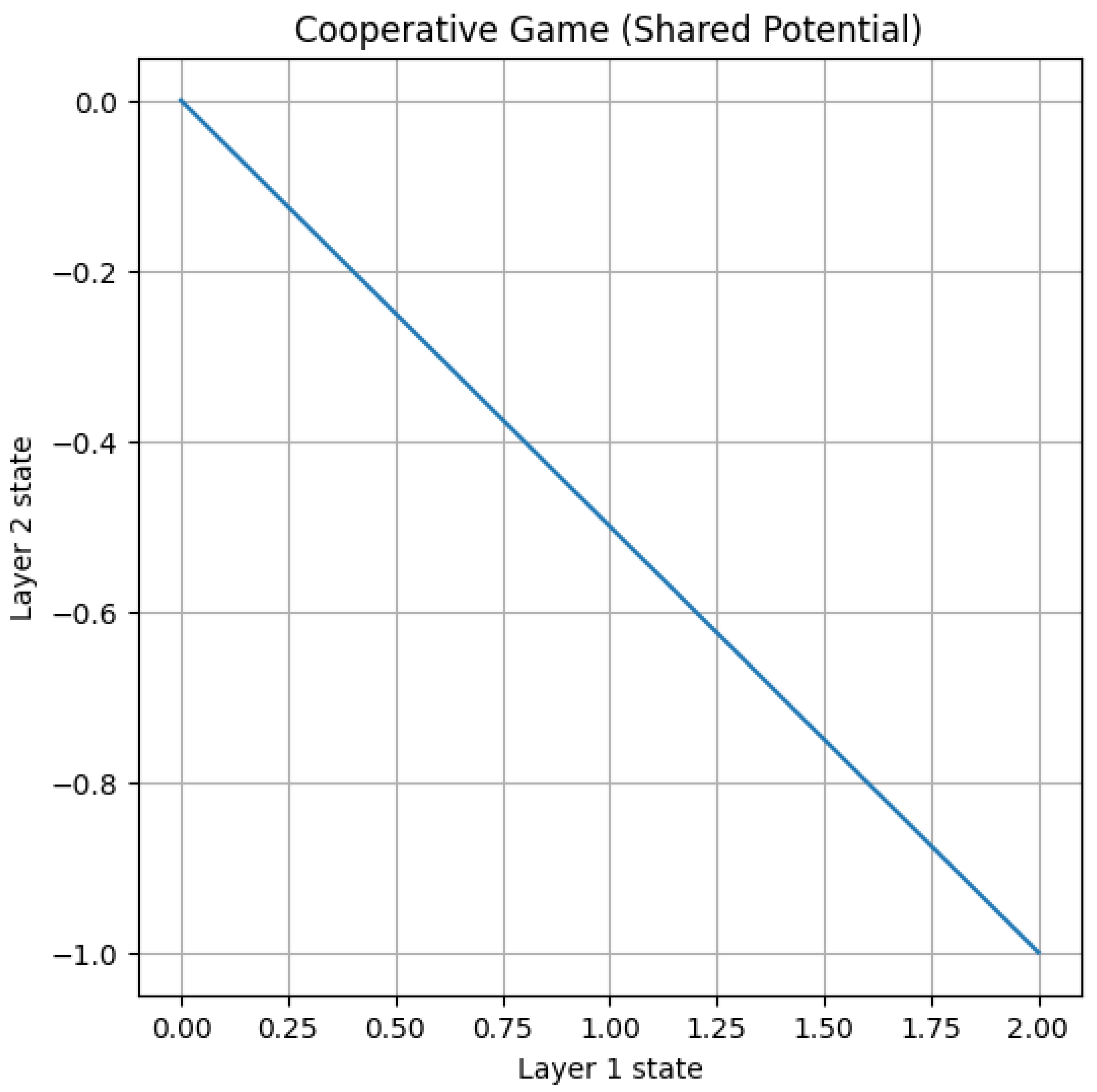
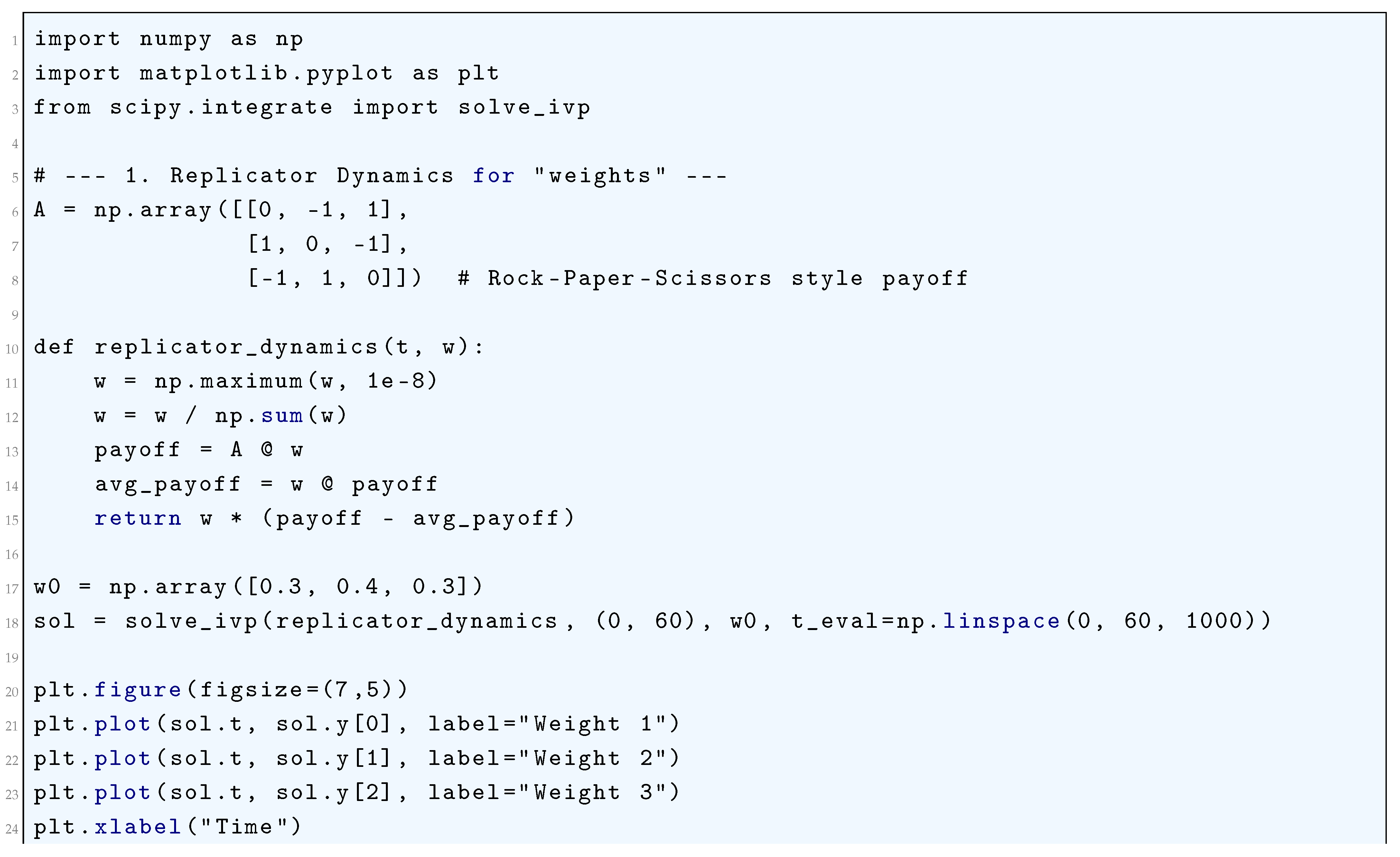
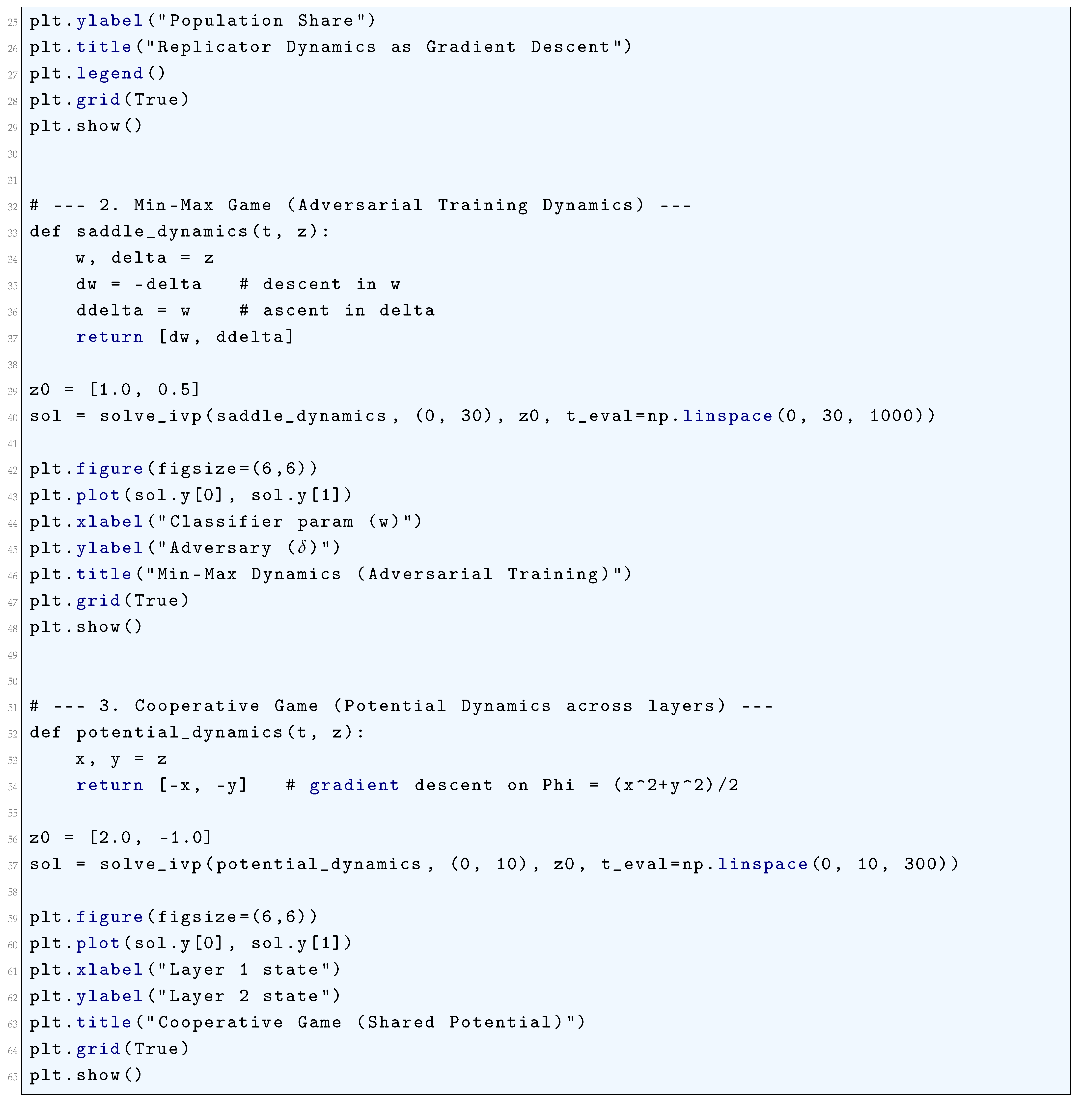
5.4. Analysis of Deep Neural Networks (DNNs) Through Variational Inequalities
Deep neural networks (DNNs) can be rigorously analyzed through the mathematical framework of variational inequalities, which provide a fundamental structure for understanding the equilibrium properties of optimization processes underlying deep learning. Variational inequalities (VIs) generalize optimization problems and offer a broader perspective on stability, convergence, and generalization in high-dimensional nonconvex settings. The problem of training a deep neural network can be formulated as a variational inequality by considering the minimization of a loss function , where the goal is to determine the optimal parameters satisfying the condition
This inequality characterizes the equilibrium conditions in the optimization landscape of deep learning. It expresses the fact that at the optimal point , any infinitesimal movement in the parameter space does not yield a lower value of the loss function. The gradient descent update rule, given by
where is the learning rate, can be rewritten as a projection-based variational inequality if constraints exist. Specifically, if the parameter space is constrained to a closed and convex set , then the variational inequality formulation of the training process is
This variational inequality expresses the fact that is a stationary point of the constrained optimization problem, meaning that the projected gradient update
ensures that the sequence converges to the solution of the variational inequality under suitable assumptions on the loss function. A key property in variational inequalities is monotonicity. The operator associated with the variational inequality is given by
and monotonicity is defined by the condition
For convex loss functions, is a monotone operator, ensuring the uniqueness of the equilibrium point. If is strongly monotone, satisfying
then the optimization process exhibits exponential convergence, meaning that the iterates satisfy
where C is a constant. This strong monotonicity property provides a rigorous foundation for understanding the rate of convergence of deep neural network training. In adversarial training, deep networks are often formulated as saddle-point problems of the form
where z represents an adversarial perturbation. The equilibrium conditions in this case are described by the system of variational inequalities
These inequalities characterize the stable equilibrium of the adversarial learning process, ensuring that neither the network nor the adversary can unilaterally improve their respective objectives. The analysis of stochastic gradient descent (SGD) in deep learning can also be conducted via variational inequalities. The expected gradient field in the presence of stochasticity is given by
where represents a random variable encoding the data distribution. The variational inequality for SGD is then
Stochastic approximation methods ensure convergence to the equilibrium point under conditions on the variance of the gradient estimator. Specifically, if is co-coercive, meaning there exists such that
then projected SGD satisfies
where is the variance of the stochastic gradient noise. This establishes a rigorous bound on the convergence rate of SGD in terms of variational inequalities. The generalization properties of deep networks can also be rigorously studied using variational inequalities. Given a distribution shift perturbation , the parameter shift satisfies the generalization bound
where the constant C is determined by the Lipschitz continuity of the gradient field. This bound ensures that the network’s performance remains stable under small perturbations in the data distribution. The variational inequality framework provides a unified perspective on optimization, equilibrium, and generalization in deep learning, offering rigorous theoretical insights into the dynamics of training and stability of neural networks.
5.4.1. Monotone/Potential Operator (Gradient of a Convex Potential)
A monotone operator is a fundamental object in the theory of variational inequalities, convex optimization, and equilibrium problems. Formally, let (H) be a real Hilbert space with inner product and induced norm . An operator is said to be monotone if for all , the inequality
holds. This condition encodes the idea that the operator does not decrease the angle between the difference of outputs and the difference of inputs, thereby generalizing the notion of a non-decreasing function in one dimension.
An important class of monotone operators arises as gradients of convex functions. Let be a convex and differentiable functional. Its gradient operator is defined by
Since is convex, it satisfies for all the first-order characterization of convexity:
Switching the roles of x and y yields
Adding these two inequalities gives
which proves that the gradient mapping is a monotone operator. Furthermore, if is strictly convex, then
which implies strict monotonicity of the operator. This property ensures uniqueness of solutions to variational inequality problems of the form: find such that
where is a convex feasible set. The monotonicity condition can also be interpreted geometrically. For the gradient of a convex function, the operator points in a direction that consistently aligns with the displacement vector between points in the domain. In other words, moving along the direction of the operator never contradicts the structure induced by convexity. This is the key mechanism underlying convergence of gradient-based algorithms in convex optimization.
In summary, the gradient of a convex potential is always a monotone operator, and the converse is also true in the sense that maximal cyclically monotone operators are precisely subdifferentials of convex functions. The equation
together with the inequality
completely captures the rigorous mathematical relationship between monotone operators and convex potentials.
5.4.2. Saddle/Non-Monotone Bilinear Operator (Models min–max Behavior)
Let , and denote . A saddle (min–max) objective is a function that is convex in x for every fixed y and concave in y for every fixed x. Associated to L one defines the operator
so that a saddle point satisfies the variational inequality
This VI formulation is equivalent to the saddle condition for all whenever (L) is convex–concave and sufficiently regular. A canonical and instructive special case is a bilinear objective
for which
The stationary (saddle) conditions and reduce to
so the solution set is ; in particular multiplicity of solutions occurs whenever (A) is rank-deficient.
For two arbitrary points and the bilinear operator satisfies the exact identity
hence (F) is (weakly) monotone in the sense that the left-hand side is identically zero for all . More generally for a smooth convex–concave L one has the monotonicity inequality
but the bilinear case is the extreme where the quantity is exactly zero rather than strictly positive.
The bilinear operator is therefore not a gradient field of any scalar potential on unless it is identically zero, because for any gradient field the Jacobian must be symmetric, whereas the Jacobian of the bilinear operator is the block matrix
which satisfies , J is skew-symmetric (block anti-symmetric) and thus cannot equal a symmetric matrix unless . Consider the continuous-time gradient-flow–ascent dynamics that arise from (F),
which for the bilinear case is the linear ODE
Because , all eigenvalues of (J) are purely imaginary (or zero); equivalently (J) generates a one-parameter family of orthogonal transformations and the quadratic energy is conserved along trajectories:
In the simplest scalar toy with one obtains , Jacobian , and the continuous dynamics
which is the harmonic oscillator; solutions are circular periodic orbits and the radius is constant in time.
The behaviour in discrete-time simultaneous gradient steps (explicit Euler) is markedly different and typically unstable. For a constant linear operator the explicit simultaneous update with step-size reads
For the scalar bilinear example the update matrix is
whose eigenvalues are and satisfy . Thus the explicit (simultaneous) method amplifies the norm and the iterates diverge for any fixed . This instability is the discrete-time manifestation of attempting to integrate a conservative rotational field with an explicit integrator: energy conservation in continuous time becomes energy growth under the explicit Euler map.
Stabilization of these rotational saddle dynamics can be achieved in several mathematically transparent ways. Adding a symmetric dissipative term (for ) to the operator, i.e. replacing by , yields a Jacobian whose symmetric part is (S) and hence the operator becomes strongly monotone with modulus at least :
Strong monotonicity implies uniqueness of the VI solution and gives (linear) contraction under appropriate implicit or proximal algorithms. Algorithmically, the extragradient method applied to a Lipschitz monotone operator F with stepsize produces the linear update for ,
and for a skew-symmetric J the term is symmetric negative semidefinite; in the scalar bilinear example giving
whose eigenvalues are and hence have modulus for consequently the extragradient step produces a contraction for sufficiently small and stabilizes the iteration where explicit simultaneous updates blow up. More generally, for monotone and L-Lipschitz operators the extragradient method converges with step-size (linear algebraic detail omitted here).
In summary, bilinear saddle operators arising in min–max problems furnish linear, skew-adjoint interaction terms that are not gradients of any scalar potential and which induce purely rotational continuous dynamics and discrete-time instabilities under naive simultaneous gradient updates. The mathematical diagnostics are
- The block-Jacobianwith
- The identityfor the bilinear case
- Conservation of quadratic energies in continuous time, and
- Discrete amplificationfor explicit Euler.
Algorithmic remedies—addition of symmetric dissipative terms, implicit/proximal discretizations, or extragradient/optimistic methods—convert the spectral properties so that the symmetric part of the Jacobian is positive (strong monotonicity) or the discrete map becomes contractive, thereby restoring convergence to equilibrium.
5.4.3. Skew (Rotation)
A skew operator is a linear operator whose defining property is antisymmetry with respect to the underlying inner product. In the setting of a finite-dimensional real Hilbert space with standard Euclidean inner product , a matrix is said to be skew-symmetric if
Equivalently, for all vectors , one has
This antisymmetry implies that the quadratic form associated with J vanishes identically, because for any
Thus, skew operators generate purely rotational effects in the vector space, preserving lengths and inner products. The eigenstructure of skew-symmetric matrices is determined by their antisymmetry. If J is real skew-symmetric, then for any eigenvalue–eigenvector pair with , one has
Taking inner products with u, it follows that
But the left-hand side vanishes since J is skew-symmetric, implying . Therefore, every eigenvalue is either zero or purely imaginary. In fact, the spectrum of J is symmetric with respect to the imaginary axis, and the nonzero eigenvalues occur in complex conjugate pairs . This fact reveals that J generates infinitesimal rotations, since purely imaginary eigenvalues correspond to circular motions.
The matrix exponential of a skew-symmetric operator describes finite rotations. For any ,
is an orthogonal matrix with determinant one, hence a rotation matrix. Orthogonality follows from the fact that
since . Thus, the flow generated by the differential equation
is given by
which traces a circular or rotational trajectory in the invariant subspaces associated with each conjugate pair of imaginary eigenvalues. The simplest case is the two-dimensional rotation operator. Let
Then the ODE expands to
which is the harmonic oscillator system. Its solution is
Thus, the trajectory is a circle centered at the origin with radius , and the motion is uniform rotation with unit angular velocity. The energy
is conserved exactly, because
In higher dimensions, skew-symmetric operators generate rotations within orthogonal two-dimensional subspaces corresponding to each pair of eigenvalues, while leaving the null space invariant. That is, decomposes into a direct sum of invariant planes where circular motions occur, and invariant lines where the dynamics are static. More explicitly, there exists an orthogonal transformation Q such that
with . Each block generates uniform rotation in its associated plane with angular speed .
The geometric effect of skew operators is thus entirely conservative: they preserve Euclidean distances and angles, merely redistributing directions through rotation. In optimization and game-theoretic dynamics, skew components in an operator correspond to cycling or rotational forces around equilibria rather than dissipative movement toward equilibria. This is reflected in the fact that monotonicity of skew operators is degenerate: for all
so skew operators are monotone but not strictly monotone. Their essential role is to encode conservative rotational dynamics rather than convergence-inducing gradients.
5.4.4. Skew + Dissipation
Let with the Euclidean inner product . Let denote a linearization of an operator F at a point (or consider the linear operator . Decompose J into its symmetric and skew-symmetric parts
with and . The phrase “Skew + Dissipation’’ refers precisely to this decomposition when S has positive semidefinite (or positive definite) character and (K) is skew-symmetric: (or with ) and . The algebraic and dynamical consequences follow from elementary identities and comparison inequalities.
For any one has the exact identity
so the skew part K does not enter the quadratic form that governs monotonicity. If then J is monotone in the sense that
and if for some then J is -strongly monotone:
Strong monotonicity immediately yields uniqueness of zeros: if and then and hence when .
Consider the continuous-time linear dynamics . The instantaneous rate of change of the quadratic energy satisfies, using the skew property ,
if . By Grönwall’s inequality this yields exponential decay
so the dissipation captured by S converts the conservative rotational action of (K) into an overall contracting flow. If with then is nonincreasing and one obtains Lyapunov stability but not exponential convergence in general.
Spectrally, if for a (complex) eigenpair then
and taking real parts gives the Rayleigh-type relation
Hence the real parts of eigenvalues of J lie in the numerical range of S; in particular implies for every eigenvalue of J. Consequently the linear semigroup generated by is exponentially stable with decay rate at least . The skew part K only shifts eigenvalues along the imaginary axis (sets the oscillation frequencies) but cannot move their real parts away from those determined by S.
In discrete time the explicit Euler map with step-size ,
is stable iff the spectral radius . The purely skew case yields eigenvalues in canonical rotational blocks and hence , so explicit steps amplify and diverge. By contrast, when (scalar dissipation and K is a rotation with frequency , the update matrix in the invariant plane is
whose eigenvalues satisfy
Thus a sufficient stability condition is
showing quantitatively how dissipation permits a finite explicit step-size that stabilizes the discrete map; when no positive suffices.
Algorithmic stabilization may also be effected by higher-fidelity integrators. The extragradient (EG) linearized update applied to a constant J produces the map
If is pure skew with on a rotation plane, then
whose eigenvalues are and hence
for sufficiently small . Thus EG introduces an effective symmetric contraction term (which is positive semidefinite when J is skew) and converts rotation into contraction; more generally for the term couples S and K and can improve stability relative to simultaneous explicit updates.
From the variational inequality viewpoint, adding dissipation upgrades monotonicity: if with and , then for the VI problem the operator is strongly monotone and the VI has a unique solution. The resolvent (proximal) operator is then a contraction: if and then
and inner-producting with and using strong monotonicity gives
hence
This resolvent contraction is the continuous-time analogue of how dissipation regularizes and guarantees stable implicit updates for nonconservative dynamics.
In summary, the mathematical role of “Skew + Dissipation’’ is: K encodes conservative rotational forces (purely imaginary spectral displacements, energy-preserving infinitesimal action) while S provides symmetric dissipation that determines real parts of the spectrum, monotonicity, energy decay, uniqueness, and contractivity. The interplay is quantitative: the magnitude of K sets frequencies and oscillation amplitudes, the minimal eigenvalue of S sets exponential decay rates in continuous time and allowable explicit step-sizes in discrete time, and algorithmic devices (EG, implicit resolvents, preconditioning) exploit the positive symmetric component or introduce effective symmetric terms to neutralize the destabilizing influence of the skew part.
5.4.5. Python Code to Generate Figure 60, Figure 61 Illustrating Monotone/Potential Operator and Figure 62 Illustrating Saddle Bilinear F (min-max) and Figure 63 Illustrating Skew (Rotation) F: R z and Figure 64 Illustrating Skew + Dissipation F: R + Alpha I
The Python code below produces the Figure 60, Figure 61 illustrating Monotone/potential operator and Figure 62 illustrating Saddle Bilinear F (min-max) and Figure 63 illustrating Skew (rotation) F: R z and Figure 64 illustrating Skew + Dissipation F: R + alpha I.
Figure 60.
Monotone/Potential F=grad Phi
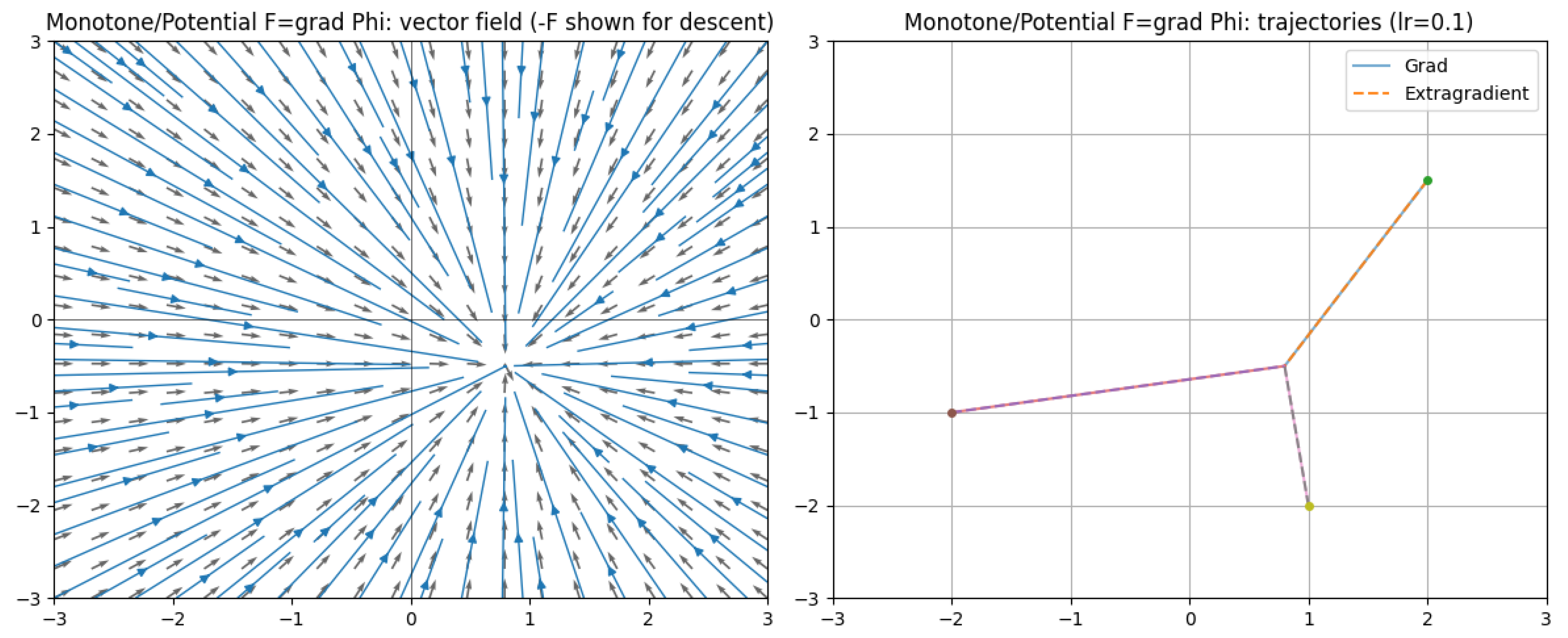
Figure 61.
Monotone case: Approx VI gap vs iteration
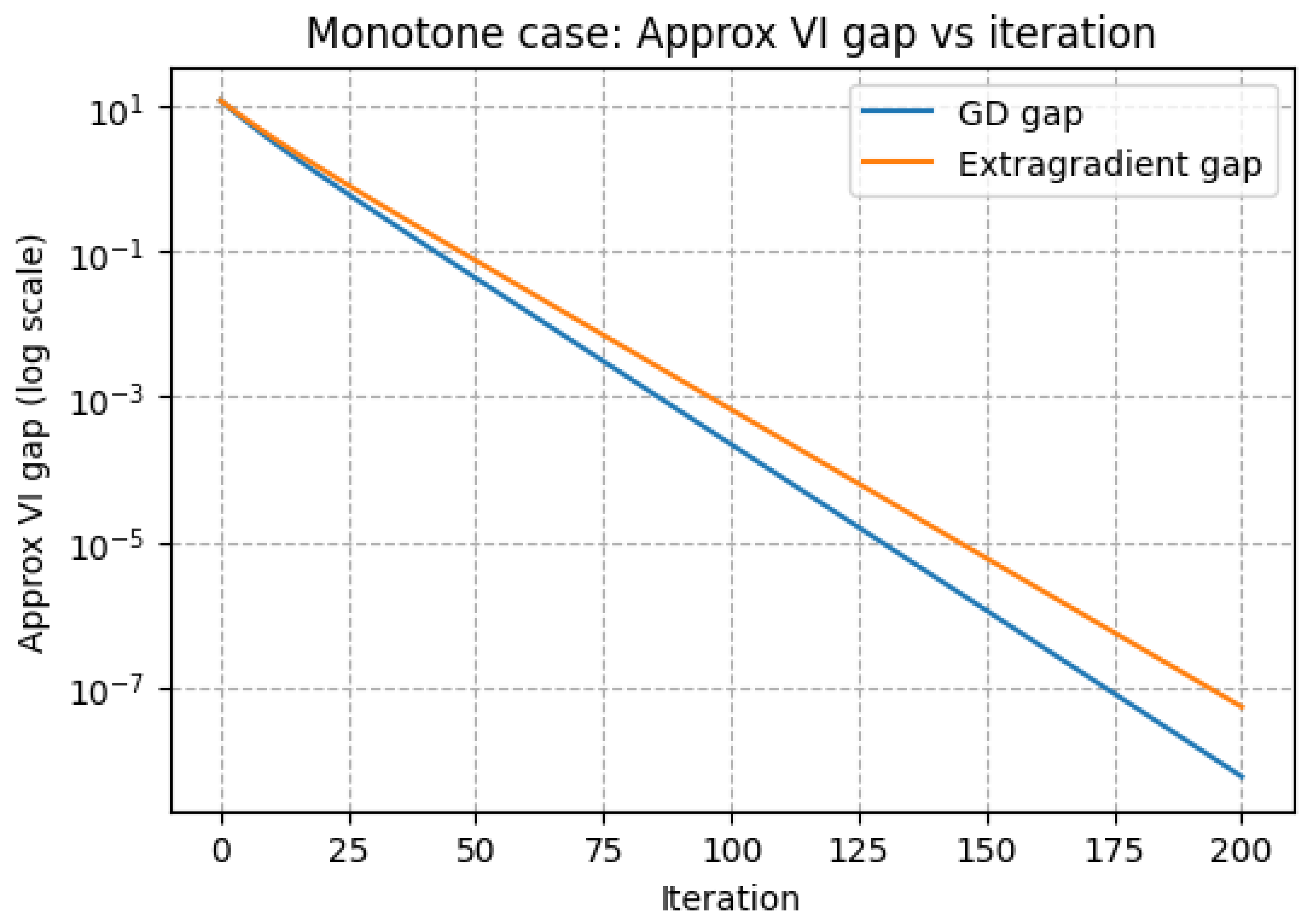
Figure 62.
Saddle Bilinear F (min-max)
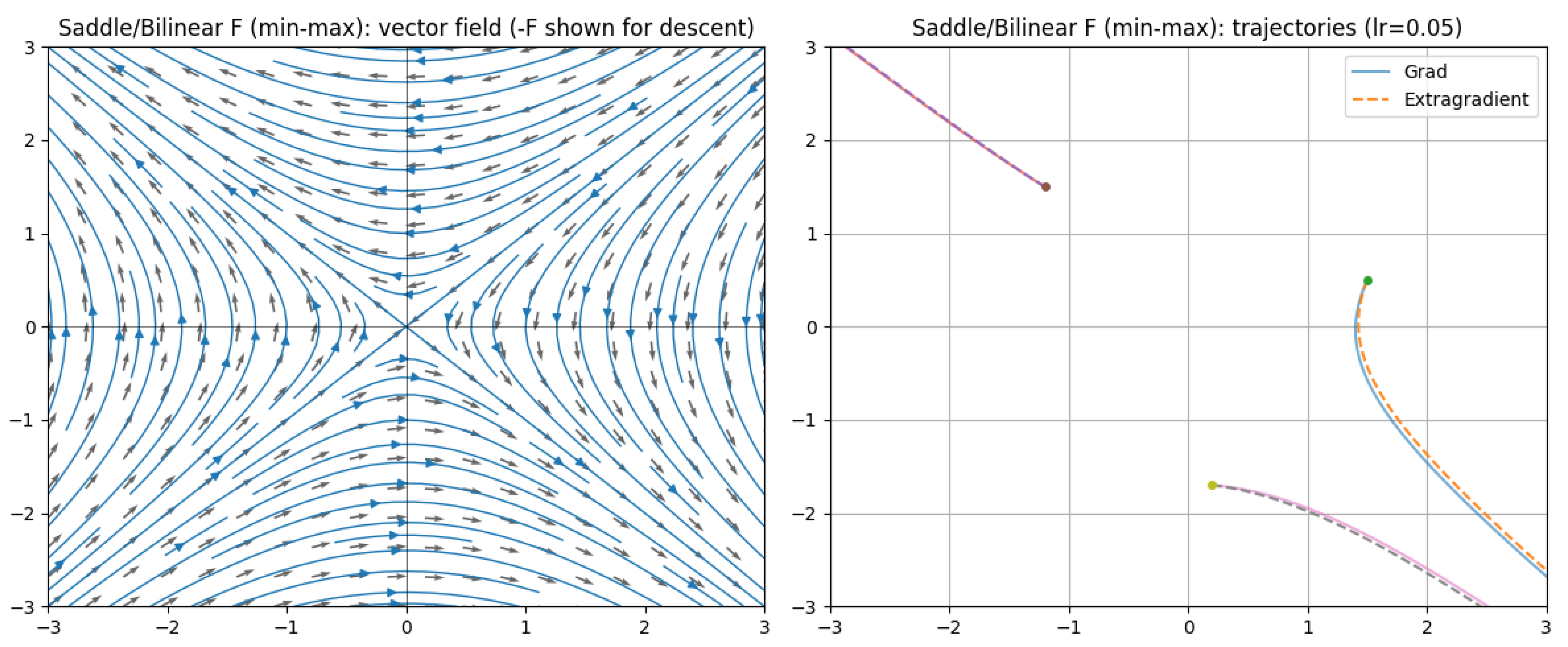
Figure 63.
Skew (rotation) F: R z
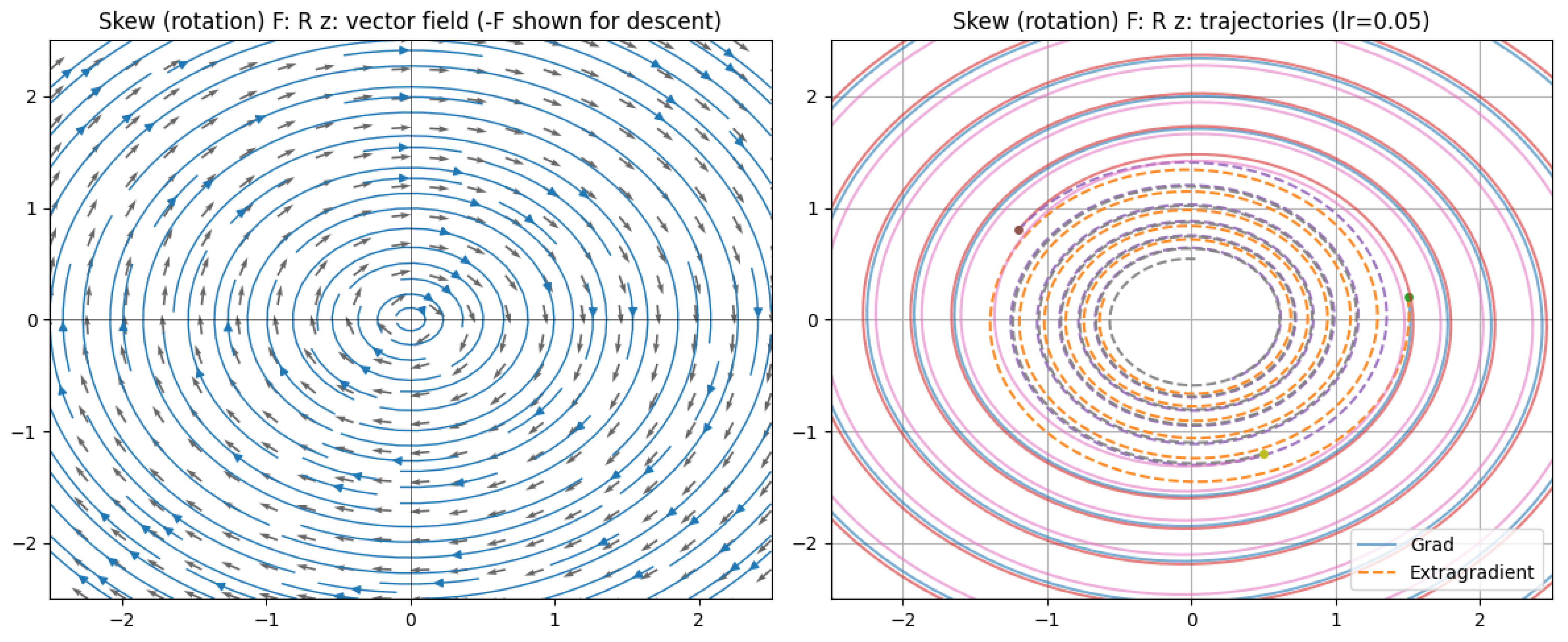
Figure 64.
Skew + Dissipation F: R + alpha I
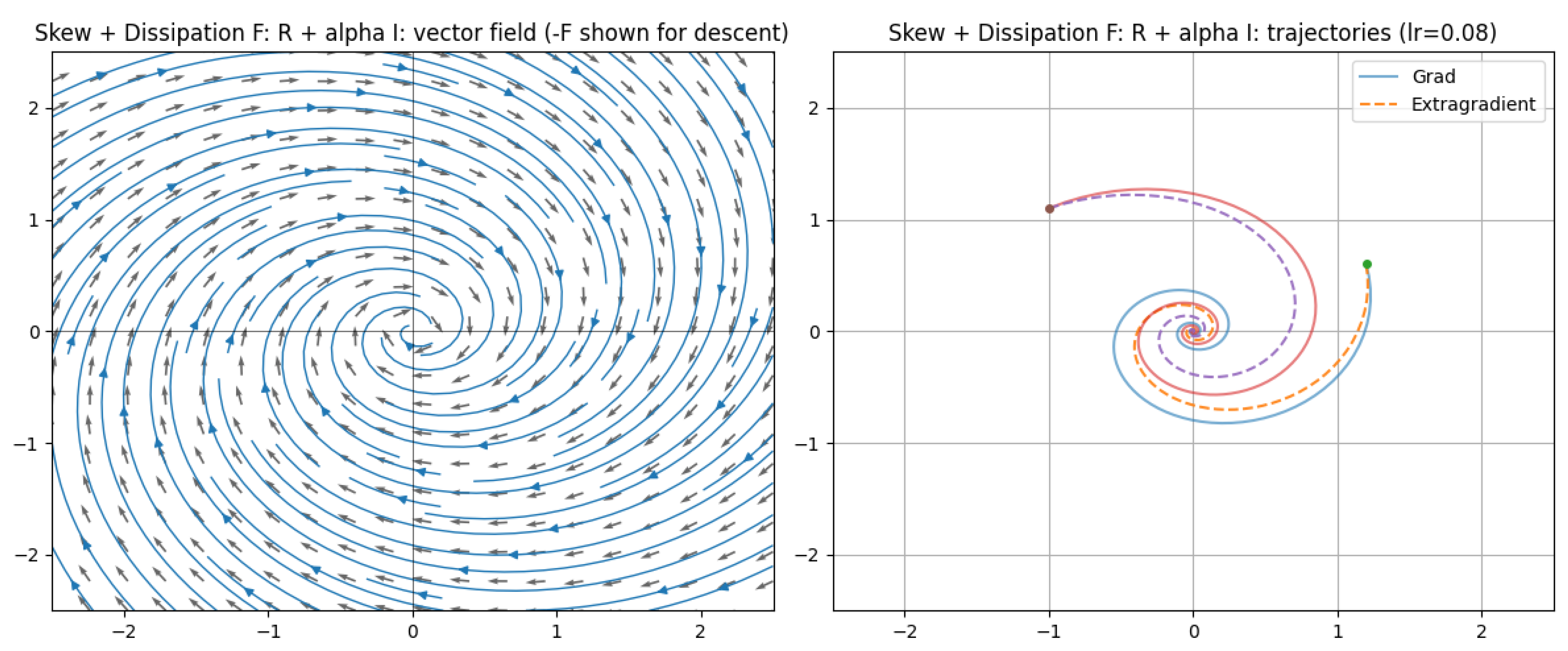
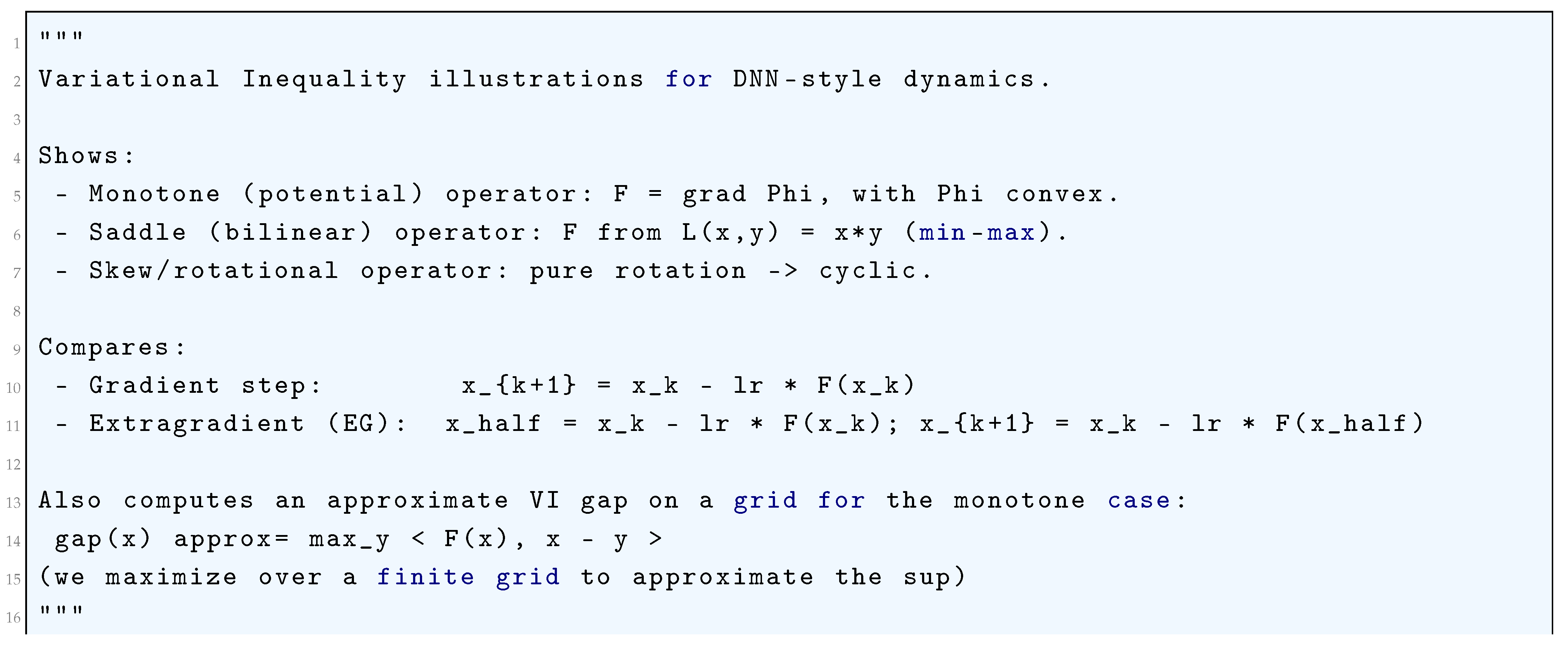
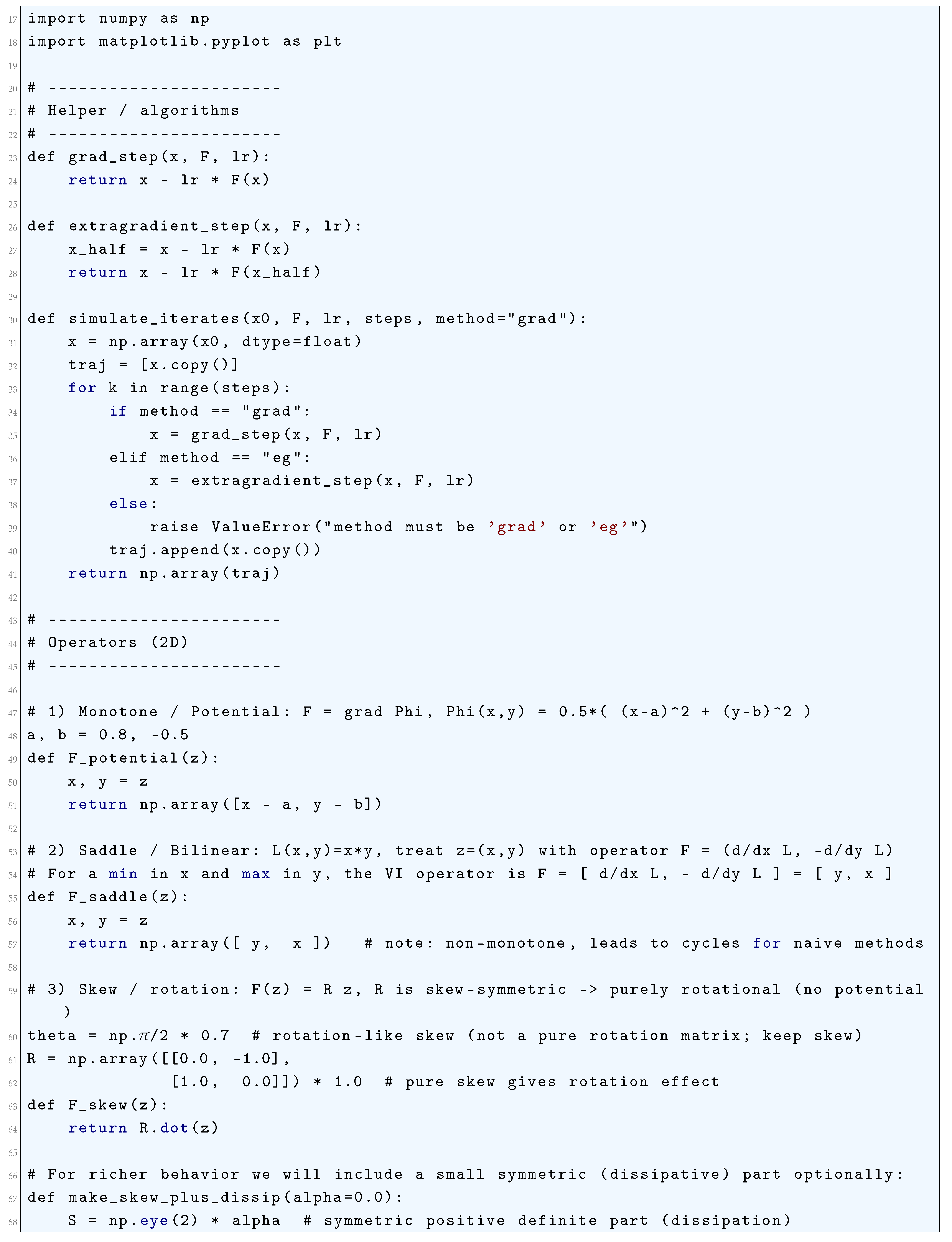
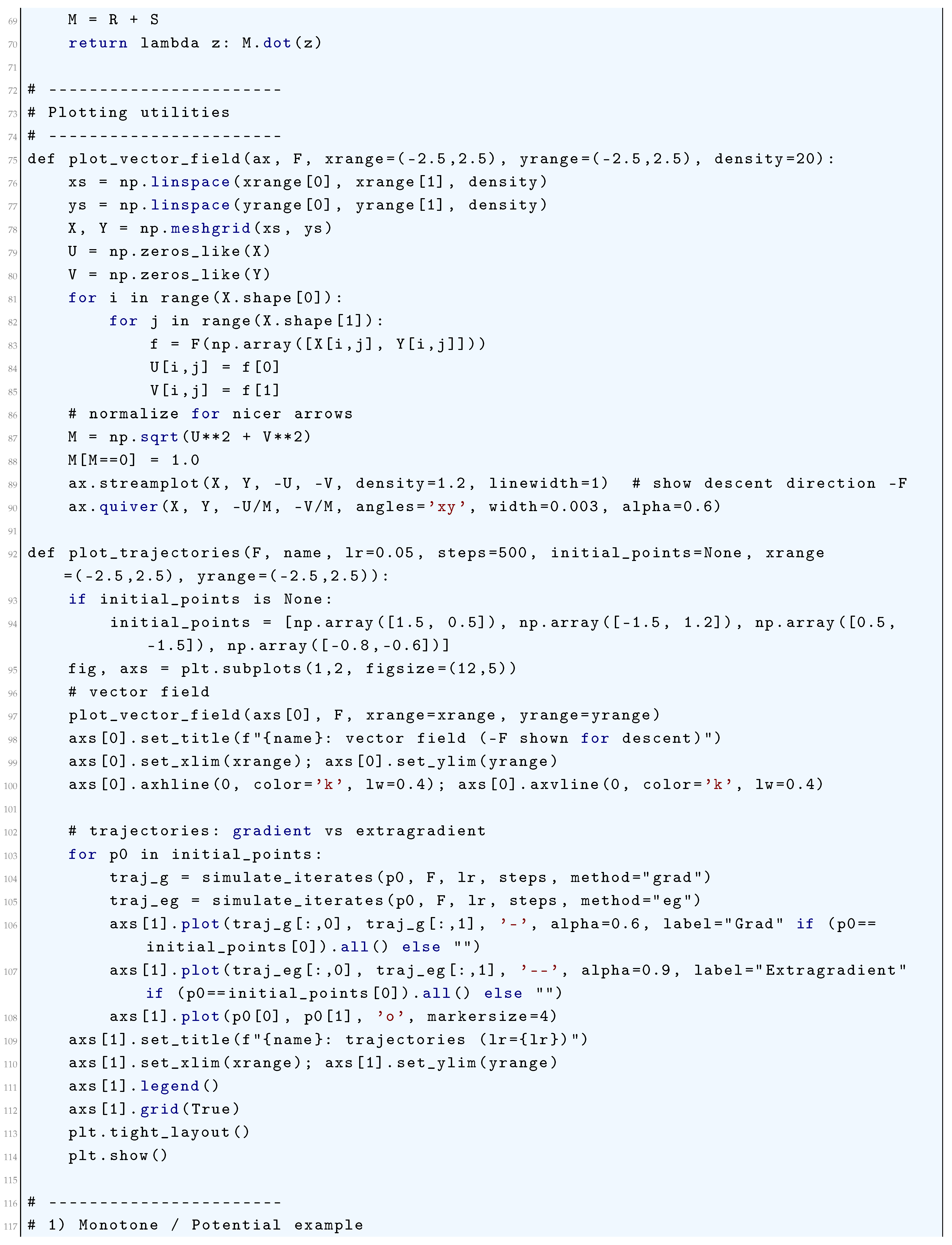
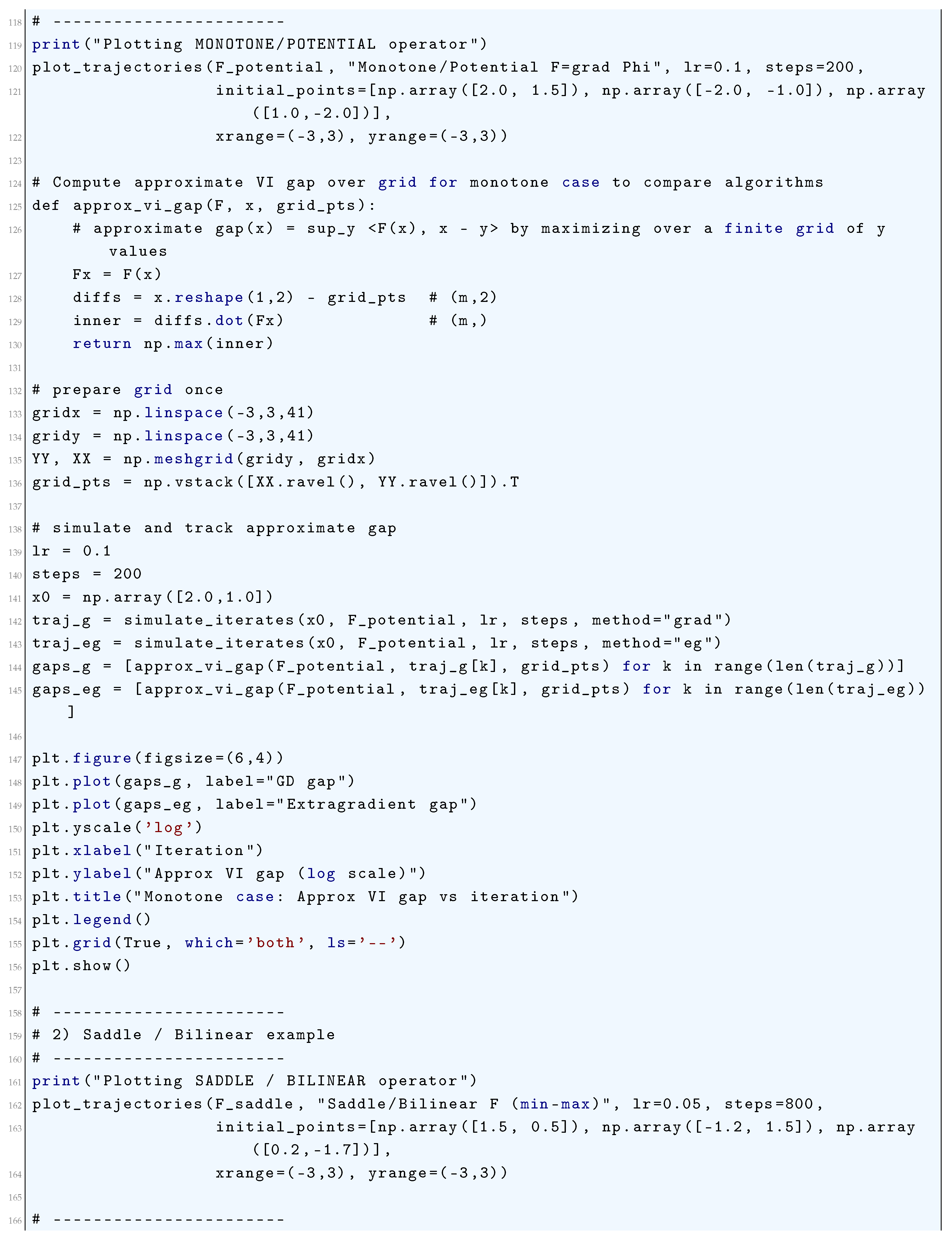
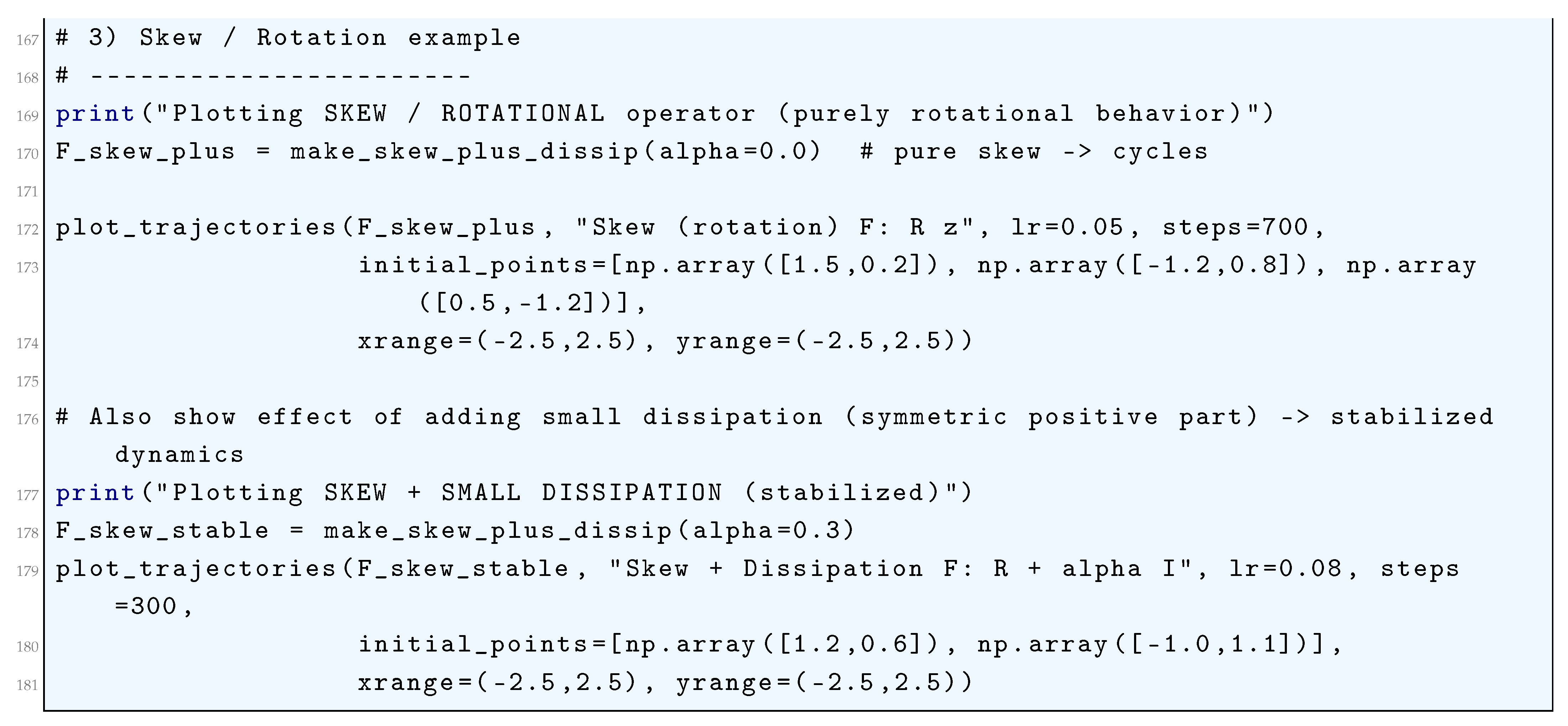
5.5. Optimal Control in Reinforcement Learning (RL)-Based Deep Neural Network (DNN) Training
Let represent the weight parameters of a deep neural network (DNN) at time step t. The evolution of these parameters over discrete time is governed by a controlled dynamical system, where the control input represents the weight update at each iteration. The fundamental objective of reinforcement learning (RL)-based DNN training is to determine an optimal control policy that minimizes a given performance criterion over a finite or infinite training horizon. The system dynamics are given by the equation
Let denote the cumulative loss function associated with a given control sequence , defined as
where is the instantaneous cost function. In the context of neural network training, the cost function is typically the empirical risk over a dataset , given by
where ℓ is a loss function such as cross-entropy or mean squared error, and represents the neural network’s output for an input x. The optimal control problem consists of finding a control sequence such that
Applying the principle of dynamic programming, the optimal cost-to-go function is defined recursively as
Expanding , the Bellman equation takes the form
Considering the continuous-time limit where the weight updates are infinitesimal, i.e., , we obtain the Hamilton-Jacobi-Bellman (HJB) equation
The optimal control satisfies
Alternatively, the problem can be analyzed using Pontryagin’s Maximum Principle. Define the Hamiltonian
where is the costate variable that evolves according to the adjoint equation
For optimality, the control must satisfy
Solving for , we obtain
In the reinforcement learning framework, the optimal control formulation is connected to policy optimization, where the policy determines the action given the state . The expected return under policy is given by
where is the reward function and is the discount factor. The policy gradient theorem states that
where is the state-action value function satisfying the Bellman equation
By applying the HJB equation, the optimal policy update rule is derived as
where is the learning rate, often adaptively adjusted based on second-order curvature information such as in natural gradient descent. More formally, using the Fisher information matrix , the optimal update rule can be written as
This establishes the link between optimal control and policy optimization in reinforcement learning, providing a rigorous theoretical foundation for RL-based DNN training.
5.5.1. Backpropagation as Pontryagin’s Maximum Principle (PMP)
We begin by formulating the supervised learning problem for a deep neural network as a discrete-time optimal control problem. Consider a network with L layers. Let the state represent the input to layer k, for . The initial state is the input data. The control variables are the parameters (weights and biases) of layer k. The state dynamics, which describe the forward propagation, are given by the equation
where is the activation function (e.g., a linear transformation followed by a non-linear element-wise function like ReLU or tanh). The objective of the training is to minimize a total cost function J that comprises a terminal cost and a running cost. The terminal cost is the loss function which measures the discrepancy between the final state (the network output) and the target label . The running cost can incorporate regularization terms on the controls, such as weight decay, leading to the full cost function
The optimal control problem is to find the sequence of controls that minimizes J subject to the dynamical constraints
Pontryagin’s Maximum Principle (PMP) provides necessary conditions for optimality for this class of problems. To apply PMP, we first define the Hamiltonian function for each stage k. The Hamiltonian is given by
where is the costate vector. The PMP states that for an optimal control sequence and the corresponding optimal state trajectory , there exists a corresponding costate trajectory satisfying the following canonical equations. The state evolution is given by the forward equation
which is identical to the network’s forward propagation. The costate evolution is governed by the backward equation
for . The boundary condition for the costate at the final time is determined by the terminal cost,
The maximization condition of PMP requires that the optimal control maximizes the Hamiltonian at every step along the optimal trajectory, that is,
for all admissible . For unconstrained controls, this often leads to the condition
which expands to
The connection to backpropagation emerges from the process of solving these necessary conditions. The standard method of successive approximation (MSA) involves a two-step iterative process. First, given a current control sequence , the state equation
is propagated forward from to to compute the state trajectory. Second, the costate equation
is propagated backward from to , initialized with
This backward pass is precisely the backpropagation algorithm. The vector is exactly the error signal, or the gradient of the loss with respect to the state , that is
The final step of MSA is to update the controls to satisfy the PMP maximization condition. For a simple case with no regularization, , the condition becomes
In practice, this condition is not enforced directly but is used to compute the gradient for a gradient-based optimizer. The gradient of the total cost J with respect to the control is given by
This is the same gradient computed by the backpropagation through time (BPTT) algorithm, where the term is the backward pass through the layer’s parameter Jacobian. Therefore, the backward pass of backpropagation is mathematically equivalent to the costate backward evolution of PMP, and the parameter gradient update is a single step (e.g., gradient ascent on the Hamiltonian) towards satisfying the PMP maximization condition. This rigorous mathematical correspondence reveals that the training of deep neural networks via gradient descent and backpropagation is an implementation of the Method of Successive Approximation for solving the necessary optimality conditions dictated by Pontryagin’s Maximum Principle.
5.5.2. The Method of Successive Approximation (MSA)
The Method of Successive Approximation (MSA) is a numerical algorithm for solving the necessary optimality conditions arising from Pontryagin’s Maximum Principle (PMP) for a discrete-time optimal control problem. In the context of training a deep neural network, the problem is formulated as minimizing a total cost
subject to the state dynamics
for , where is the input data, is the network output, is the target, are the parameters of layer k, and is a regularization function. The Hamiltonian for this system is defined as
where is the costate variable. The PMP provides the necessary conditions for optimality: the state equation
the costate equation
with the boundary condition
and the maximization condition
for all admissible , which for unconstrained, differentiable problems implies the stationarity condition
or explicitly
The MSA algorithm iteratively refines a sequence of control policies to satisfy these conditions. Given an initial guess for the control sequence for , the i-th iteration of MSA consists of two sequential passes. The first pass is the forward state propagation, which computes the state trajectory corresponding to the current control guess . This is executed by initializing with the input data and recursively applying the dynamics
for to . This forward pass is identical to a forward propagation through the neural network using the current parameters. The second pass is the backward costate propagation, which computes the costate trajectory using the computed states and controls . This pass is initialized with the gradient of the terminal loss
and proceeds backwards recursively using the costate equation
for . This backward pass is mathematically equivalent to the backpropagation algorithm, as the costate represents the negative gradient of the total cost with respect to the state,
The third and final step of the MSA iteration is the control update, which aims to satisfy the PMP maximization condition. A new control sequence is computed to maximize the Hamiltonian given the newly computed states and costates . The update is performed pointwise for each k by solving
For the common case where the dynamics are differentiable with respect to and the regularization is convex, the maximization condition leads to the implicit equation
which expands to
Solving this equation exactly for is often computationally intractable. Instead, a common approximation is to perform a single gradient ascent step on the Hamiltonian with respect to the control. This involves computing the gradient
and then updating the controls as
where is a learning rate. Crucially, the gradient is precisely the negative of the gradient required to minimize the total cost J, since
when the state and costate equations are satisfied. Therefore, the control update
is recovered, which is the standard gradient descent update used in backpropagation-based training. Thus, the MSA algorithm, with a single gradient step for the control update, is mathematically equivalent to the training of a deep neural network via forward propagation, backpropagation of errors, and a gradient descent step on the parameters, providing a rigorous optimal control interpretation of the entire learning process. The iteration continues until a convergence criterion on the control sequence or the total cost is met, yielding a solution that approximates the PMP necessary conditions.
5.5.3. Differentiable Optimization Layers
Differentiable Optimization Layers represent a profound integration of mathematical optimization into the fabric of deep neural networks, where the output of a layer is defined as the solution to a constrained optimization problem. The forward pass of such a layer, at a given depth k, computes the state by solving a parameterized problem:
where is a cost function internal to the layer, is a constraint set defined by parameters (the previous state) and (the layer’s control parameters or weights), and is the optimization variable. This formulation generalizes standard layers; for example, a linear layer followed by a ReLU activation can be interpreted as solving a quadratic program with non-negativity constraints. The primary challenge lies in differentiating through this argmin operation to compute the Jacobians and required for the backward pass during training. This is not a standard application of the chain rule because the mapping from parameters to solution is implicitly defined by the optimality conditions of the optimization problem.
The rigorous treatment of backpropagation through these layers relies on the implicit function theorem applied to the Karush-Kuhn-Tucker (KKT) conditions. For a convex optimization problem with inequality constraints, the Lagrangian is
where represents the inequality constraints, represents the equality constraints, and , are the dual variables. The KKT optimality conditions, which must hold at the solution , are stationarity:
primal feasibility:
dual feasibility:
and complementary slackness:
where ⊙ denotes the Hadamard product. The implicit function theorem states that if the Jacobian of the system of equations formed by the stationarity and active constraints with respect to the primal and dual variables is invertible at the solution, then the solution and the active dual variables are differentiable functions of the parameters .
To compute the necessary gradients for the backward pass, we consider the total derivative of the loss function ℓ with respect to the parameters. Let be the incoming gradient from the subsequent layer, which is the negative costate from the PMP viewpoint. The goal is to compute
and
Differentiating the system of KKT conditions that hold at the optimum with respect to the parameters provides a linear system to solve for these Jacobians. Let represent the concatenated vector of the primal variable and the dual variables for the active constraints (where is the set of indices for which and ). The active KKT conditions form a system
which includes the stationarity condition and the active equality constraints
The total derivative is
which yields
The Jacobian is the KKT matrix at the optimum. The desired Jacobian is a block of .
A more efficient and direct method, which avoids explicitly forming and inverting the full KKT matrix, involves solving a linear system that yields the gradient directly. The differential of the stationarity condition is
where and . Expanding this differential with respect to perturbations , , and the resulting changes , , gives:
where
is the Hessian of the Lagrangian with respect to . Simultaneously, the differentials of the active constraints must be zero:
and
This can be written as a linear system:
To compute the vector-Jacobian product , one sets to be the identity in the direction of interest and solves the adjoint of this system. The standard approach is to solve for the adjoint variables such that:
The solution to this adjoint system then gives the desired gradient with respect to the previous state:
An analogous procedure, solving a similar adjoint system but with the right-hand side terms derived from differentiation with respect to , yields the gradient . This formalism provides a complete and rigorous mechanism for embedding optimization problems as differentiable layers within a deep network, allowing for end-to-end training using gradient-based methods while maintaining a direct interpretation as an optimal control step within the network’s dynamics.
5.5.4. Neural Ordinary Differential Equations (Neural ODEs)
Neural Ordinary Differential Equations (Neural ODEs) formulate the forward propagation through a deep neural network as the solution to a continuous-time dynamical system defined by an ordinary differential equation. The state of the network, represented by a vector , evolves from an initial time to a final time according to the differential equation
where is a function parameterized by the network weights , and the initial condition is the input data . The output of the network is the state at the terminal time, . This formulation generalizes residual networks, where each layer performs an update
to the continuous limit as the number of layers approaches infinity and the step size approaches zero. The fundamental problem of training such a network is an optimal control problem, where the goal is to find the control parameters that minimize a loss function subject to the dynamical constraint of the ODE. The cost functional is
where is a running cost, often a regularization term on the weights or the state.
The necessary conditions for optimality are derived from the calculus of variations and Pontryagin’s Maximum Principle in continuous time. The Hamiltonian for this system is defined as
where is the costate variable. The PMP states that for an optimal control and the corresponding optimal state trajectory , there exists a costate trajectory satisfying the canonical equations. The state equation is the forward ODE:
The costate equation is the backward ODE:
with the terminal boundary condition
The optimality condition for the control requires that the Hamiltonian is maximized, leading to
for all .
The central innovation for training Neural ODEs is the adjoint sensitivity method, which provides a memory-efficient way to compute the gradient of the loss with respect to the parameters, , by solving a backward ODE. The adjoint state is defined as , which is exactly the negative of the costate, . Its dynamics are derived by differentiating the loss with respect to time. Consider the total derivative
However, ℓ is a constant function of t, so . A more rigorous derivation considers the gradient
from the PMP and constructs an augmented state
whose dynamics can be computed backwards. The definitive result is that the adjoint state satisfies the differential equation
with the initial condition
To compute the total gradient , an auxiliary variable is introduced, which evolves as
with . The total gradient is then
In practice, the forward pass is performed by numerically integrating the ODE
from to using an ODE solver to obtain the final state and the loss . The backward pass does not require storing the intermediate states of the forward pass. Instead, the combined adjoint system is solved backwards in time from to . The system to be solved is defined for the augmented state
and its dynamics are given by:
The initial conditions for this backward integration are
and
Crucially, to compute the right-hand side of this adjoint ODE, the state trajectory is required. It can be recomputed backwards from by solving the original ODE backwards, or more efficiently, it can be reconstructed during the backward pass if a reversible ODE solver is used, or by using a continuous-time checkpoints and interpolation based on the solver’s internal steps. The final value provides the necessary gradient for updating the parameters via gradient descent. This entire procedure, where the backward pass is computed by solving a differential equation, is a direct and rigorous implementation of the continuous-time PMP, establishing Neural ODE training as a canonical example of optimal control in deep learning. The absence of a discrete computational graph for backpropagation allows for adaptive computation and constant memory cost relative to depth, as the memory requirement is instead of for a network with L layers.
5.5.5. Stochastic Optimal Control for RL and Robust Training
Stochastic Optimal Control provides the foundational framework for Reinforcement Learning by considering dynamical systems governed by stochastic differential equations or Markov Decision Processes, where the state evolution incorporates inherent uncertainty. The continuous-time formulation models the state dynamics as
where is the state, is the control, is a standard Wiener process representing Brownian motion, and is the diffusion matrix. The objective is to find a control policy that minimizes the expected cost
where is the terminal cost and is the running cost. The fundamental equation of stochastic optimal control is the Hamilton-Jacobi-Bellman equation, a nonlinear partial differential equation for the optimal value function
The HJB equation is derived via the dynamic programming principle and Itô’s lemma, yielding
with the terminal condition . The term is the second-order differential operator arising from the variance of the Brownian motion, which is absent in deterministic control.
The connection to Reinforcement Learning emerges from the discrete-time, finite-horizon formulation known as a Markov Decision Process, defined by the tuple , where is the state space, is the action space, is the transition probability kernel, is the reward function, and is the discount factor. The objective is to maximize the expected discounted return
The optimal value function
satisfies the discrete-time HJB equation, known as the Bellman optimality equation:
Similarly, the optimal state-action value function
provides the basis for Q-learning algorithms. Policy iteration and value iteration are dynamic programming algorithms that solve these equations, and when the state and action spaces are large, deep neural networks are used as function approximators, leading to Deep RL. The parameters of a value network or a policy network are trained to minimize the Bellman error
or to maximize the expected return
using the policy gradient theorem
For robust training of deep neural networks in supervised learning, the problem is framed as a minimax game or a robust optimal control problem where the controller must perform well under worst-case perturbations. Given a training dataset , the dynamics of a deterministic network are
and the objective is to minimize the loss . In the presence of adversarial perturbations applied to the input or intermediate features, the robust training problem is
where is a bounded set of admissible perturbations, such as . This can be viewed as a zero-sum dynamic game where nature chooses the worst-case disturbance. The Hamiltonian for this robust control problem incorporates the disturbance
and the robust optimality conditions involve a maximization over the disturbance followed by a minimization over the control. Solving the inner maximization exactly is often intractable, leading to approximations like Projected Gradient Descent to find adversarial examples
which are then used in training, a method known as Adversarial Training.
A more formal approach uses stochastic control theory with uncertain dynamics. The dynamics are modeled as
where is a random noise vector. The goal is to find a control policy that minimizes the expected loss while being robust to the noise distribution. This leads to risk-sensitive optimal control, which optimizes a risk-measure of the cost, such as the exponential utility
where is a risk-aversion parameter. Using the Taylor expansion
it is clear this penalizes high variance in the loss. The Path Integral Control framework provides a solution for a specific class of stochastic problems where the dynamics are affine in the control and the cost is quadratic in the control. For a system with dynamics
and cost
the HJB equation can be linearized via a logarithmic transformation
leading to a linear PDE for . The optimal control is then given by
which can be estimated by sampling trajectories, forming the basis of the Model Predictive Path Integral (MPPI) control algorithm used in RL for policy improvement. This direct sampling-based approach bypasses the need for value function approximation and is highly suitable for complex, high-dimensional problems where DNNs represent the policy.
5.5.6. Stable and Efficient Network Design
The design of stable and efficient neural networks from an optimal control perspective necessitates the enforcement of structural constraints on the network’s dynamics to guarantee desirable properties such as Lyapunov stability, passivity, or contractivity, which in turn ensure robustness to input perturbations and prevent exploding gradients during training. Consider the discrete-time dynamical system representation of a neural network
where is the state and are the parameters. A fundamental stability concept is that of a contraction mapping, which requires the existence of a matrix measure such that the Lipschitz constant of each layer is strictly less than one, , ensuring that the distance between any two trajectories contracts over time. A more general and powerful framework is provided by Lyapunov theory. A Lyapunov function for the autonomous system
must satisfy for all and , and the condition
for some , guaranteeing global exponential stability of the equilibrium point. To design layers that inherently satisfy such properties, one can parameterize the layer as the solution to a constrained optimization problem or as the forward Euler discretization of a continuous-time system with known stability properties.
A prominent approach is to design layers that are nonexpansive, meaning they are 1-Lipschitz continuous
for all which prevents the amplification of input perturbations and gradient norms. This can be achieved by constraining the weights to be orthogonal or using spectral normalization, which enforces
where denotes the maximum singular value. A more rigorous method involves modeling the network as the discretization of a continuous-time Ordinary Differential Equation
and ensuring the continuous dynamics are contractive. A nonlinear system is contractive if there exists a uniformly positive definite metric
such that the generalized Jacobian
is uniformly negative definite, i.e.,
for some . A sufficient condition for contractivity in the identity metric is that the symmetric part of the Jacobian is uniformly negative definite
This insight leads to the design of stable continuous-time blocks, such as
where is a monotone activation function, which can be shown to be contracting under certain conditions on .
The training of such stable architectures can be framed as an optimal control problem with stability constraints. The objective is to minimize the loss
subject to the dynamics
and the algebraic stability constraints , where encodes constraints like spectral norm bounds. The Lagrangian for this constrained optimization is
where are the Lagrange multipliers for the stability constraints. The necessary conditions from the Karush-Kuhn-Tucker theorem include the state equation
the costate equation
with
and the stationarity condition with respect to the controls
complemented by the complementary slackness conditions
In practice, the stability constraints are often enforced via projected gradient descent or by reparameterizing the weights. For example, one can parameterize a weight matrix as
where has its spectral norm constrained to 1 via iterative power methods, and is a trainable scalar, ensuring
For recurrent networks and those with skip connections, more advanced concepts from robust control, such as the use of Linear Matrix Inequalities (LMIs), are required to guarantee stability. Consider a system with uncertain or time-varying parameters,
where , a bounded uncertainty set. The system is quadratically stable if there exists a matrix such that the LMI
holds for all . This can be extended to nonlinear systems via sector bounds on the activation functions. Let be a slope-restricted activation function in the sector , meaning
for all . A network layer
can be analyzed using the discrete-time version of the Kalman-Yakubovich-Popov lemma. Stability can be certified by finding a diagonal positive definite matrix and a matrix such that the following LMI is feasible:
Training a network to satisfy such LMIs during optimization is challenging but can be approximated by incorporating a regularization term that penalizes the violation of the stability condition, leading to a robust and stable network architecture whose training dynamics are themselves well-behaved, mitigating issues like vanishing and exploding gradients and enhancing generalization performance by enforcing a smooth input-output map. The integration of these control-theoretic stability constraints directly into the architecture and the training loop represents a principled approach to designing deep neural networks with predictable and reliable behavior, which is paramount for their deployment in safety-critical reinforcement learning applications.
5.5.7. Optimal Control of the Training Process Itself
The optimal control of the training process itself constitutes a meta-optimization problem where the parameters of the learning algorithm, such as the learning rate, momentum coefficients, or even the entire update rule, become the control variables in a higher-level dynamical system whose state is the entire set of model parameters and optimizer states. Let represent the parameters of the deep neural network at optimization step t, and let represent the state of the optimizer, which may include momentum vectors , variance estimates , and other auxiliary variables. The combined state is
The update rule of the optimizer defines the dynamics of this meta-system. For a generic optimizer, the dynamics can be expressed as
where is a vector of hyperparameters (e.g., learning rate, momentum decay factor) acting as the control signal, and
is the stochastic gradient computed on a minibatch at step t. The fundamental challenge is that the gradient is not an exogenous input but a function of the state and the data distribution, making the system a closed-loop feedback system with stochastic disturbances.
The objective of the meta-optimization is to find a hyperparameter policy
that minimizes the expected total loss over a horizon T, which is
where is a discount factor. This is a classic stochastic optimal control problem. The corresponding Bellman equation for the optimal meta-value function is
where the expectation is over the stochasticity in the gradient . The optimal hyperparameter control is then
Solving this exactly is intractable, but it provides a formal framework for gradient-based hyperparameter optimization. By considering the hyperparameters as fixed over a horizon, one can compute the hypergradient to perform meta-descent. This involves differentiating through the optimization process. The dynamics for a simple gradient descent optimizer are
The hypergradient for a horizon of one step is trivial:
For a longer horizon T, the hypergradient requires backpropagation through the entire training trajectory (through-time), given by
where
and
is the Hessian at step k, and
This product of Hessians is computationally prohibitive and numerically unstable, leading to approximations such as ignoring the higher-order terms and using the approximation
For more complex optimizers like Momentum or Adam, the state and its dynamics become crucial. The momentum optimizer has states and dynamics
where the controls are . The hypergradient for the learning rate involves differentiating through these dynamics:
where
This creates a recurrent system for the hypergradient that mirrors the parameter update itself. The Adam optimizer introduces further complexity with states , and dynamics
where the division and square root are element-wise. Differentiating through this requires careful application of the chain rule, and the hypergradients for , , and can be computed recursively, albeit with significant memory and computational cost if done exactly through a long horizon.
A more general and rigorous approach formulates this as a continuous-time optimal control problem for the training trajectory. The parameters evolve during training "time" according to the optimizer’s ODE, such as
for gradient flow. The meta-control problem is to find the time-varying learning rate that minimizes
The Hamiltonian for this meta-problem is
where is the meta-costate. The meta-costate equation is
with the terminal condition . The optimality condition for the control is
implying that the optimal learning rate is chosen such that the meta-costate is orthogonal to the gradient. This continuous-time formulation elegantly captures the trade-off: the term in the costate dynamics represents the interaction between the learning rate and the curvature of the loss landscape, guiding how should be adjusted to navigate sharp minima and flat regions effectively. This rigorous optimal control perspective provides a unifying theoretical foundation for understanding and designing adaptive learning rate schedules and other meta-optimization strategies, framing the entire training procedure of a deep neural network as a single, coherent control problem over the space of parameters.
5.5.8. Connections to Reinforcement Learning
The connections between optimal control and reinforcement learning are foundational and profound, with RL being essentially a framework for solving stochastic optimal control problems in the absence of a known dynamical model. The canonical formulation is the Markov Decision Process defined by the tuple , where is the state space, is the action space, is the transition probability kernel, is the reward function, and is the discount factor. The objective is to find a policy that maximizes the expected discounted return
The optimal value function
satisfies the Bellman optimality equation
which is the discrete-time, stochastic analogue of the Hamilton-Jacobi-Bellman equation from continuous optimal control. The Hamiltonian for the discrete MDP can be defined as
and the Bellman equation is then
directly mirroring the HJB condition
for the deterministic case.
Policy iteration and value iteration are the dynamic programming algorithms that solve the Bellman equations, and when the state and action spaces are large, function approximation is required, leading to Deep Reinforcement Learning where deep neural networks parameterize the value function or the policy . The training of these networks is itself an optimal control problem where the parameters or are the controls, and the dynamics are defined by the optimization algorithm. The value network parameters are trained to minimize the expected Temporal Difference error, which is derived from the Bellman equation. The TD error for a transition is
and the mean-squared projected Bellman error objective is
The gradient of this objective is
which can be seen as a stochastic gradient descent update aiming to satisfy the Bellman orthogonality condition, a form of policy evaluation in the linear function approximation setting.
For policy-based methods, the policy gradient theorem provides the foundational update rule. The objective is
where is a trajectory and
The policy gradient is
A more common and lower-variance form uses the state-action value function
yielding
where is the stationary state distribution under policy . This gradient can be interpreted from an optimal control perspective where the policy update is a step towards maximizing a performance metric, and the Q-function acts as a costate-like variable that evaluates the quality of the action. Advanced policy gradient methods like Trust Region Policy Optimization (TRPO) and Proximal Policy Optimization (PPO) explicitly incorporate a constraint on the policy change, framing the update as a constrained optimization problem
subject to
where
is the advantage function. This is a direct application of a trust-region method in the policy space, ensuring stable and monotonic policy improvement, which is a form of robust control against overly large policy updates.
The connection is further solidified in model-based reinforcement learning and planning. When a model of the environment dynamics is learned or known, optimal control methods can be directly applied for planning. The learned dynamics model , often parameterized by a deep neural network, allows the use of trajectory optimization techniques like Model Predictive Control (MPC) and the Linear Quadratic Regulator (LQR). For a finite horizon H, the goal is to find an action sequence that minimizes
The iLQR algorithm solves this by iteratively linearizing the dynamics around a nominal trajectory and quadratizing the cost, leading to a locally optimal linear feedback policy
The dynamics are linearized as
where
and the cost is quadratized as
The iLQR backward pass then computes the value function
recursively from to using the Riccati equations
and the optimal feedback gain is
with the value function parameters updated as
This direct application of optimal control provides a powerful planning algorithm that can be used to generate targets for policy and value network training, creating a hybrid model-based and model-free RL system where the strengths of both optimal control theory and deep learning are synergistically combined.
5.6. Differential Game Theory and Training Dynamics
Differential game theory provides a rigorous mathematical framework for analyzing the continuous-time dynamics of competing or cooperating agents in deep learning systems, such as generative adversarial networks (GANs), multi-agent reinforcement learning, and adversarial training. Consider a game with K players, where each player k controls a parameter vector that evolves in time according to a differential strategy. The collective state of the system is described by the joint trajectory , governed by coupled ordinary differential equations (ODEs) derived from gradient-based optimization:
Here, denotes the loss function for player k, which may be adversarial (e.g., in GANs) or cooperative (e.g., in distributed optimization). The dynamics are influenced by the interaction matrix , a block-structured Jacobian encoding pairwise competition or cooperation:
The eigenvalues of determine stability: if all eigenvalues have negative real parts, the system converges to a Nash equilibrium; if any are positive, instability or limit cycles may emerge, as observed in GAN training.
In the special case of zero-sum games (e.g., GANs), the dynamics can be reformulated as a Hamiltonian system, where the total "energy" is conserved along trajectories. Let denote the generator and discriminator parameters, respectively. The Hamiltonian dynamics are given by:
This formulation reveals oscillatory behavior when , explaining cyclic divergence in GANs. Alternatively, training dynamics can be analyzed via Wasserstein gradient flows, where parameter updates approximate the gradient flow of a functional in probability space. For a loss over a parameter distribution , the continuity equation describes its evolution:
where is the functional derivative. This perspective connects deep learning to mean-field theory, explaining phenomena like mode collapse and implicit regularization via the geometry of parameter distributions. The interplay between differential game theory and training dynamics thus provides a unified framework for understanding optimization, stability, and convergence in complex learning systems.
6. Optimal Transport Theory in Deep Neural Networks
Optimal transport (OT) theory provides a rigorous geometric framework for comparing probability distributions and has become a foundational tool in analyzing and training deep neural networks (DNNs). Given two probability measures and defined on metric spaces and , respectively, the Monge-Kantorovich problem seeks a transport plan that minimizes the expected cost of moving mass from to :
where is a cost function (e.g., Euclidean distance ), and denotes the set of joint distributions with marginals and . The optimal transport distance, or Wasserstein distance, quantifies the minimal effort required to reconfigure into :
In deep learning, OT is employed to align latent representations, regularize generative models, and define loss functions for distribution matching. For instance, Wasserstein GANs (WGANs) replace the Jensen-Shannon divergence with the 1-Wasserstein distance , leading to improved training stability:
where D is a 1-Lipschitz discriminator enforcing the Wasserstein constraint.
The computational complexity of OT motivates approximations such as entropy-regularized transport, where the Kantorovich problem is relaxed with a Kullback-Leibler (KL) divergence penalty:
The Sinkhorn algorithm solves this efficiently via iterative scaling, enabling scalable OT-based losses in DNNs. The Sinkhorn divergence, a debiased version of , is given by:
which is positive definite and avoids the bias of entropy smoothing. This divergence is used in tasks like domain adaptation, where source and target distributions and are aligned by minimizing for a feature map .
OT theory also informs the design of neural architectures through dynamic transport perspectives. The continuity equation describes the evolution of a parameter distribution under gradient flow:
where is the velocity field induced by the loss functional . This links to the Benamou-Brenier formula, which expresses as an infimum over kinetic energy:
subject to . In deep learning, this inspires Neural ODEs and normalizing flows, where layers are viewed as discretized OT maps. For example, a residual block approximates an infinitesimal transport along , with the network trained to minimize the OT cost between input and output distributions.
OT theory further provides mechanisms for geometric regularization via barycenters. Given distributions , their Wasserstein barycenter minimizes:
where are convex weights. In DNNs, this facilitates multi-task learning by interpolating between task-specific distributions in latent space. The barycentric projection of a transport plan also defines a mapping , used in style transfer and cross-domain alignment.
By embedding OT principles into deep learning, models gain robustness to distributional shifts, improved generative fidelity, and theoretically grounded training dynamics, bridging measure theory and neural optimization.
6.1. Literature Review of Optimal Transport Theory in Deep Neural Networks
Optimal transport theory has become a cornerstone in the analysis and design of deep neural networks, providing a rigorous framework for understanding geometric and probabilistic aspects of learning. Peyré and Cuturi (2019) [1515] offer a comprehensive introduction to the mathematical foundations of optimal transport, with a focus on computational aspects that are crucial for scaling these methods to high-dimensional spaces encountered in deep learning. Its contribution lies in bridging theoretical optimal transport with practical algorithms, enabling applications such as Wasserstein barycenters and gradient flows in neural network training. Santambrogio (2015) [1518] provides a rigorous treatment of the analytical aspects of optimal transport, including Kantorovich duality and Monge-Ampère equations, which are essential for understanding the geometric regularization effects of Wasserstein distances in neural networks. This text is particularly valuable for its deep mathematical insights into how transport-based losses can stabilize and improve generalization in deep models. Arjovsky et al. (2017) [1459] revolutionized generative modeling by introducing the Wasserstein distance as a loss function, addressing the vanishing gradients and mode collapse issues in traditional GANs. This work rigorously establishes the connection between optimal transport and adversarial training, showing how the Wasserstein metric provides a meaningful gradient signal even when the supports of the distributions are disjoint. Gulrajani et al. (2017) [1473] further refine this approach by proposing gradient penalty methods to enforce the Lipschitz constraint, a key technical contribution that ensures stable training. These works collectively demonstrate how optimal transport theory can lead to more robust and interpretable generative models. Frogner et al. (2015) [1508] explore the statistical properties of Wasserstein-based learning, providing generalization bounds and approximation guarantees for neural networks trained with optimal transport objectives. This work is foundational for understanding the trade-offs between expressivity and sample complexity in transport-based deep learning.
Villani (2009) [1521] offers a deep dive into the geometric and probabilistic aspects of optimal transport, with implications for understanding the latent space geometry of neural networks. Its contribution lies in connecting abstract measure-theoretic concepts to practical questions about how neural networks transform and interpolate between distributions. Cuturi (2013) [1505] introduces entropy-regularized optimal transport, a breakthrough that enables efficient computation of Wasserstein distances in high dimensions. This work is particularly impactful for deep learning, as it allows scalable training of models with optimal transport losses. Genevay et al. (2018) [1509] extend these ideas to generative modeling, showing how Sinkhorn divergences can be used to train variational autoencoders with improved sample quality. These contributions highlight the interplay between computational optimal transport and deep generative modeling. Taghvaei and Jalali (2019) [1519] propose a neural network-based approach to solving optimal transport problems, effectively learning the transport map as a parameterized function. This represents a significant shift from traditional linear programming methods, enabling scalable solutions to high-dimensional transport problems. Tolstikhin et al. (2018) [1520] introduce a framework for auto-encoder training based on optimal transport, providing a principled way to balance reconstruction accuracy and latent space regularization. This work is notable for its rigorous treatment of the connection between variational inference and Wasserstein distances. Ramdas et al. (2017) [1517] develop statistical tests based on optimal transport, with applications to evaluating generative models and detecting distributional shifts in deep learning. These contributions demonstrate the versatility of optimal transport in addressing fundamental challenges in neural network training and evaluation.
Ambrosio et al. (2008) [1503] provide a rigorous foundation for understanding gradient-based optimization in the space of probability measures, which is crucial for analyzing the dynamics of neural network training through the lens of optimal transport. Its contribution lies in formalizing the connection between Wasserstein gradient flows and optimization algorithms used in deep learning. Mei et al. (2018) [1513] apply optimal transport theory to analyze the convergence of stochastic gradient descent in overparameterized neural networks, showing how the particle dynamics can be described as a Wasserstein gradient flow. This work bridges the gap between theoretical optimal transport and practical deep learning optimization. Janati et al. (2020) [1511] extend optimal transport theory to handle mismatched masses, a common scenario in deep learning where distributions may not be normalized. This technical advancement enables more flexible applications of transport-based methods in neural networks. Evans (2021) [1507] surveys the broad landscape of optimal transport theory, with particular emphasis on its connections to partial differential equations and variational problems. This work is invaluable for understanding how transport-based regularization can influence the solutions learned by neural networks. Courty et al. (2017) [1504] introduce a framework for adapting neural networks across domains using Wasserstein distances, providing rigorous guarantees on target domain performance. This contribution is particularly impactful for transfer learning and unsupervised domain adaptation. Li et al. (2015) [1512] explore the relationship between optimal transport and kernel-based discrepancies, offering insights into alternative distributional metrics for generative modeling. These works collectively expand the toolbox of transport-based methods available for deep learning applications.
Rachev and Rüschendorf (1998) [1516] provide encyclopedic coverage of optimal transport theory, with extensive treatment of its probabilistic and statistical aspects. This reference is essential for understanding the measure-theoretic foundations of Wasserstein distances in neural network analysis. Deshpande et al. (2018) [1506] introduce computationally efficient approximations to optimal transport by projecting distributions onto random directions, enabling scalable training of generative models. This work represents an important practical advancement in making transport-based methods feasible for large-scale deep learning. Ozair et al. (2019) [1514] develop a transport-based dependency metric that can be used to regularize neural network representations, contributing to the field of disentangled representation learning. These contributions demonstrate the growing influence of optimal transport across various subfields of deep learning. Richards et. al. (2020) [222] provided an intuitive introduction to modeling Rayleigh–Bénard convection within a stochastic framework, emphasizing understanding over mathematical rigor. It outlines how stochastic processes such as Brownian motion and stochastic differential equations can be applied to model convective phenomena. The work serves as a conceptual and computational guide for developing numerical simulations of stochastic fluid dynamics systems. Huang et al. (2021) [1510] propose a method for constructing explicit transport maps in generative models, providing both theoretical guarantees and practical algorithms. This work bridges the gap between normalizing flows and optimal transport theory. The convergence analysis of transport-based optimization in deep learning is further advanced by rigorous studies connecting Wasserstein geometry with stochastic gradient descent dynamics. The interplay between optimal transport and deep learning continues to inspire new theoretical insights and algorithmic innovations, shaping the future of machine learning research and applications.
6.2. Analysis of Optimal Transport Theory in Deep Neural Networks
Optimal transport theory provides a mathematically rigorous framework for measuring distances between probability distributions by solving a constrained optimization problem that minimizes the cost of transporting mass from one distribution to another. Consider two probability measures and defined on a common measurable space , where has support and has support . Given a cost function , the optimal transport problem seeks to determine a transport plan that minimizes the total cost of transforming into . In the Monge formulation, this problem is expressed as
subject to the constraint that the transport map T satisfies the push-forward condition
which ensures that the measure is obtained by pushing forward through T, i.e., for any measurable set ,
The Monge problem is often ill-posed since a transport map may not exist. To alleviate this issue, the Kantorovich relaxation introduces a coupling between and , where is a probability measure on satisfying the marginal constraints
The Kantorovich formulation of the optimal transport problem is thus
where is the set of all couplings satisfying the marginal constraints. A commonly used cost function is the p-th power of the Euclidean distance, i.e., , which leads to the Wasserstein distance of order p, given by
The Wasserstein distance defines a proper metric on the space of probability measures, provided that and have finite p-th moments, i.e.,
In deep neural networks, optimal transport plays a crucial role in generative modeling, where it provides a more stable alternative to divergence-based training objectives. In Wasserstein generative adversarial networks (WGANs), the standard Jensen-Shannon divergence is replaced by the Wasserstein-1 distance, leading to the objective
where f is a Lipschitz-1 function, is the real data distribution, is the latent distribution, and is the generator function. The use of the Wasserstein distance improves gradient behavior and mitigates mode collapse, which is a common issue in standard GAN training. In domain adaptation, optimal transport is used to align source and target distributions by finding a transport plan that minimizes the Wasserstein distance between them. Given a source distribution and a target distribution , the goal is to find a transport map T such that
which is often achieved by solving
To ensure computational efficiency, entropy-regularized optimal transport introduces a regularization term based on the Kullback-Leibler divergence, leading to the Sinkhorn distance
The regularization parameter controls the trade-off between accuracy and computational efficiency. The Sinkhorn algorithm, which iteratively updates the dual potentials using Bregman projections, provides an efficient means of computing approximate solutions to the OT problem. Optimal transport has also been applied to learning energy-based models, where it is used to define a structured loss function for training probability models. In probabilistic autoencoders, OT distances provide a principled approach for matching latent and data distributions. In Bayesian deep learning, OT-based priors ensure that posterior distributions maintain smooth and stable representations, improving generalization in uncertainty estimation tasks. The OT-based barycenter problem arises in multi-modal learning, where the goal is to compute a central distribution that minimizes the sum of Wasserstein distances to a set of given measures . The barycenter is defined as
which generalizes the notion of averaging to probability distributions. Applications of OT barycenters include meta-learning, ensemble methods, and federated learning, where a global model must aggregate information from multiple local distributions while minimizing divergence. The theoretical properties of optimal transport, including dual formulations and regularity results, provide strong guarantees for its application in deep neural networks. The dual formulation of the Wasserstein distance is given by the Kantorovich-Rubinstein theorem, which states that for ,
This dual representation allows gradient-based optimization methods to efficiently approximate OT distances in neural network training. Furthermore, recent advances in computational optimal transport, including sliced Wasserstein distances and entropic maps, have enabled scalable implementations suitable for high-dimensional deep learning applications.
Optimal transport thus provides a fundamental mathematical framework for distributional matching in deep learning. By leveraging Wasserstein distances and entropy-regularized formulations, OT enables more stable training, improved generalization, and better interpretability in neural networks, making it an essential tool for modern deep learning methodologies.
6.3. Jensen-Shannon Divergence
The Jensen-Shannon divergence (JSD) is a rigorously defined, symmetric, and bounded measure of dissimilarity between two probability distributions P and Q. It is constructed from the Kullback-Leibler divergence (KLD) but incorporates a mixture distribution to ensure symmetry and finiteness. The JSD is defined as:
where M is the average distribution of P and Q, given by:
Here, and are the Kullback-Leibler divergences between P and M, and Q and M, respectively. The KLD for two discrete probability distributions P and M is defined as:
where and are the probabilities assigned to the i-th event by P and M, respectively. For continuous probability distributions, the KLD is expressed as:
where and are the probability density functions of P and M, respectively. Substituting the definition of M into the JSD, we obtain:
For continuous distributions, this becomes:
The JSD can also be expressed in terms of Shannon entropy. Let denote the Shannon entropy of P, defined for discrete distributions as:
For continuous distributions, the differential entropy is:
Using entropy, the JSD can be rewritten as:
This formulation demonstrates that the JSD measures the difference between the entropy of the average distribution M and the average of the entropies of P and Q. The JSD is bounded between 0 and 1 when the logarithm base is 2, as:
The lower bound is achieved when , and the upper bound is approached when P and Q are maximally different. The square root of the JSD is a metric, satisfying the triangle inequality:
for any probability distribution R. This property makes the JSD particularly useful in applications requiring a distance metric, such as clustering and classification. The JSD is also related to the total variation distance by the inequality:
This relationship connects the JSD to other statistical distances, providing a bridge between information-theoretic and measure-theoretic perspectives. The JSD is widely used in machine learning, bioinformatics, and statistics due to its symmetry, boundedness, and interpretability. It is particularly useful for comparing empirical distributions, as it avoids the infinite values that can arise with the KLD. The JSD can also be generalized to compare more than two distributions. For n distributions , the generalized JSD is:
This generalization retains the properties of the standard JSD, including symmetry and boundedness. The JSD is also closely related to the concept of mutual information, as it can be interpreted as the mutual information between a random variable and a mixture distribution. Specifically, for two distributions P and Q, the JSD can be expressed as:
where X is a random variable with distribution P or Q, and Y is a binary indicator variable selecting between P and Q. This interpretation provides a deeper understanding of the JSD as a measure of information overlap. In summary, the Jensen-Shannon divergence is a versatile and mathematically rigorous tool for quantifying the difference between probability distributions, with applications across numerous scientific and engineering disciplines. Its properties make it a preferred choice in many scenarios where symmetric and bounded divergence measures are required.
6.4. Matching Latent and Data Distributions in Probabilistic Autoencoders
Optimal Transport (OT) distances provide a mathematically rigorous framework for comparing probability distributions, making them particularly suitable for aligning latent and data distributions in Probabilistic Autoencoders (PAEs). The core idea of OT is to find the most efficient way to transform one distribution into another, where efficiency is quantified by a cost function. In the context of PAEs, this translates to minimizing the discrepancy between the encoded latent distribution and the prior distribution , as well as between the decoded data distribution and the true data distribution .
Let and be two probability measures defined on metric spaces and , respectively. The OT problem seeks a coupling that minimizes the total transportation cost:
where is a cost function, typically the Euclidean distance for . The p-Wasserstein distance is a special case of OT, defined as:
In PAEs, the latent distribution is often modeled as a Gaussian , and the prior is typically a standard Gaussian . The OT distance between these distributions can be computed using the 2-Wasserstein distance, which has a closed-form expression for Gaussian distributions:
For the decoded data distribution , the OT distance to the true data distribution can be approximated using discrete OT methods. Given samples from and from , the empirical OT problem becomes:
where and are empirical measures. The coupling is a doubly stochastic matrix satisfying and . The OT distance can be incorporated into the PAE objective function as a regularization term. The overall loss function combines the reconstruction loss and the OT-based regularization:
where and are hyperparameters controlling the strength of the regularization terms. The first term ensures accurate reconstruction, while the second and third terms enforce consistency between the latent and prior distributions, and between the decoded and true data distributions, respectively. The OT framework also allows for the use of entropy-regularized OT, which introduces a regularization term to the OT problem to make it computationally tractable. The entropy-regularized OT problem is given by:
where is the entropy of the coupling , and is the regularization parameter. This formulation leads to the Sinkhorn algorithm, which provides an efficient way to compute approximate OT distances.
In summary, OT distances offer a principled and mathematically rigorous approach for matching latent and data distributions in PAEs. By minimizing the Wasserstein distance between distributions, PAEs can achieve better alignment between the encoded latent space and the prior, as well as between the decoded data and the true data distribution. This results in more robust and interpretable models, with improved generative and reconstructive capabilities.
6.4.1. Probabilistic Autoencoders
Probabilistic autoencoders are generative models that combine the principles of autoencoders with probabilistic frameworks to learn a latent representation of data. Let be the observed data, and be the latent variable, where . The goal is to model the joint distribution , which can be factorized as:
Here, is the prior distribution over the latent space, often chosen as a standard Gaussian , and is the likelihood function, which models the data generation process. The encoder in a probabilistic autoencoder approximates the posterior distribution , which is typically intractable. Instead, a variational distribution is introduced, parameterized by , to approximate the true posterior. This distribution is often chosen as a Gaussian , where and are outputs of a neural network. The decoder, parameterized by , models the likelihood , which is also often Gaussian for continuous data:
The learning objective is to maximize the marginal likelihood , which can be expressed as:
However, this integral is intractable due to the high-dimensional latent space. Instead, the evidence lower bound (ELBO) is maximized, which is derived using variational inference:
The first term in the ELBO is the reconstruction loss, which encourages the model to accurately reconstruct the input data. The second term is the Kullback-Leibler (KL) divergence between the variational posterior and the prior , which regularizes the latent space to match the prior distribution. The ELBO can be rewritten as:
where and are the mean and variance of the i-th dimension of the latent variable . The parameters and are optimized using stochastic gradient descent. The expectation term in the ELBO is approximated using Monte Carlo sampling. For a single sample , the ELBO can be approximated as:
To enable backpropagation through the sampling process, the reparameterization trick is used. Specifically, is reparameterized as:
where and ⊙ denotes element-wise multiplication. This allows gradients to flow through the sampling process, enabling efficient optimization. The reconstruction loss depends on the type of data. For continuous data, it is often the negative log-likelihood of a Gaussian distribution:
For binary data, the Bernoulli distribution is used, and the reconstruction loss becomes:
where is the i-th element of the reconstructed data . The KL divergence term can be computed analytically for Gaussian distributions. For a standard Gaussian prior and a Gaussian variational posterior , the KL divergence is:
If the variational posterior is diagonal, i.e., , the KL divergence simplifies to:
The optimization of the ELBO is performed using gradient-based methods. The gradients of the ELBO with respect to and are computed using automatic differentiation. For a mini-batch of data , the stochastic gradient estimate of the ELBO is:
where . The probabilistic autoencoder can be extended to more complex architectures, such as hierarchical models with multiple layers of latent variables. In such cases, the latent variables are structured hierarchically, and the joint distribution is factorized as:
where are the latent variables at different levels of the hierarchy. The variational posterior is also factorized hierarchically:
The ELBO for hierarchical models includes additional KL divergence terms for each level of the hierarchy:
In summary, probabilistic autoencoders provide a principled framework for learning latent representations of data by combining the strengths of autoencoders and probabilistic models. The ELBO serves as the optimization objective, balancing reconstruction accuracy and regularization of the latent space. The reparameterization trick enables efficient gradient-based optimization, and the framework can be extended to hierarchical models for more complex data structures.
6.4.2. 2-Wasserstein Distance
The 2-Wasserstein distance, also known as the Earth Mover’s Distance (EMD) in the case of , is a metric used to quantify the difference between two probability distributions and defined on a metric space . It is a specific instance of the more general p-Wasserstein distance, which is defined for . The 2-Wasserstein distance is particularly significant due to its geometric interpretation and its applications in optimal transport theory, statistics, and machine learning.
Given two probability measures and on X, the 2-Wasserstein distance is defined as the infimum of the expected squared distance between random variables X and Y, where X is distributed according to and Y is distributed according to , over all possible joint distributions of with marginals and . Mathematically, this is expressed as:
where denotes the set of all joint probability measures on with marginals and , i.e., for any measurable sets , and . The distance is the metric on the space X, and the integral represents the expected squared distance under the coupling . The 2-Wasserstein distance can also be expressed in terms of the cumulative distribution functions (CDFs) of and when . Let and be the CDFs of and , respectively. Then, the 2-Wasserstein distance is given by:
where and are the quantile functions (inverse CDFs) of and , respectively. This formulation is particularly useful in one-dimensional settings, as it reduces the problem to computing the integral of the squared difference between the quantile functions. In the case where and are absolutely continuous with respect to the Lebesgue measure, with probability density functions and , the 2-Wasserstein distance can be related to the optimal transport map T that pushes forward to , i.e., . The map T minimizes the transport cost:
The optimal transport map T is often characterized by the Monge-Ampère equation, which relates the densities and through the Jacobian determinant of T:
In higher dimensions, the 2-Wasserstein distance is more challenging to compute, but it can be approximated using numerical methods such as linear programming, entropic regularization, or Sinkhorn iterations. The dual formulation of the 2-Wasserstein distance, derived from Kantorovich duality, provides another perspective:
where the supremum is taken over all pairs of continuous functions and on X satisfying the constraint:
This dual formulation is particularly useful in theoretical analyses and provides a connection to convex optimization. The 2-Wasserstein distance has several important properties, including symmetry, non-negativity, and the triangle inequality, making it a true metric on the space of probability measures with finite second moments. It is also sensitive to the geometry of the underlying space X, as it incorporates the metric directly into its definition. This geometric sensitivity makes it particularly useful in applications such as image processing, where the spatial arrangement of pixels is crucial.
In summary, the 2-Wasserstein distance is a powerful tool for comparing probability distributions, with deep connections to optimal transport theory, convex analysis, and geometry. Its rigorous mathematical formulation and rich theoretical properties make it a cornerstone of modern probability and statistics.
6.5. Optimal Transport (OT)-Based Priors in Bayesian Deep Learning
The incorporation of Optimal Transport (OT)-based priors into Bayesian Deep Learning frameworks ensures that posterior distributions maintain smooth and stable representations by leveraging the rigorous mathematical properties of the Wasserstein distance and its associated geometric structure. This approach is grounded in measure theory, functional analysis, and convex optimization, providing a robust foundation for uncertainty estimation tasks. Below, we provide a deeper and more mathematically rigorous exposition.
Let be a complete separable metric space, and let denote the space of probability measures on X with finite p-th moments. For , the p-Wasserstein distance is defined as:
where is the set of all couplings (joint distributions) with marginals P and Q. The Wasserstein distance induces a metric on , endowing it with a geometric structure that is sensitive to the underlying topology of X. This sensitivity ensures that the Wasserstein distance captures not only global but also local differences between distributions, making it particularly suitable for regularizing posterior distributions in Bayesian inference. In Bayesian Deep Learning, the prior and the posterior are probability measures over the parameter space . To ensure smoothness and stability of the posterior, we introduce an OT-based regularization term into the variational inference objective. Specifically, we augment the evidence lower bound (ELBO) with a Wasserstein penalty:
where is a regularization hyperparameter, and is the Kullback-Leibler divergence. The Wasserstein term enforces geometric consistency between the prior and the posterior, ensuring that the posterior does not deviate excessively from the prior in a manner that respects the underlying metric structure of . The smoothness of the posterior is guaranteed by the properties of the Wasserstein distance. Specifically, the Wasserstein distance is Lipschitz-continuous with respect to perturbations in the distributions. For any , the triangle inequality holds:
This inequality ensures that small changes in the data distribution D or the prior lead to proportionally small changes in the posterior , thereby promoting stability. Furthermore, the Wasserstein distance is convex in its arguments, which facilitates efficient optimization and guarantees the existence of a unique minimizer under appropriate conditions. To compute the Wasserstein distance in practice, we often employ entropic regularization, which transforms the OT problem into a strictly convex optimization problem. The entropic regularized Wasserstein distance is defined as:
where is the entropy of the coupling , and is the regularization parameter. The entropic regularization ensures that the optimal coupling is unique and has the form:
where f and g are dual potentials that satisfy the Schrödinger system of equations. This formulation allows for efficient computation using the Sinkhorn-Knopp algorithm, which iteratively updates the dual potentials f and g. The stability and smoothness of the posterior are further reinforced by the dual formulation of the Wasserstein distance. By the Kantorovich-Rubinstein duality, the 1-Wasserstein distance can be expressed as:
where is the set of 1-Lipschitz functions on X. This dual formulation highlights the role of Lipschitz continuity in controlling the smoothness of the posterior, as the Wasserstein distance penalizes functions that vary too rapidly.
In summary, OT-based priors ensure that posterior distributions maintain smooth and stable representations by leveraging the geometric and analytical properties of the Wasserstein distance. The Wasserstein distance provides a rigorous framework for regularizing Bayesian inference, ensuring that the posterior remains close to the prior in a geometrically meaningful way. This approach is computationally tractable due to entropic regularization and the Sinkhorn-Knopp algorithm, and it is theoretically grounded in measure theory, convex analysis, and functional analysis. The resulting Bayesian framework is robust to noise and distributional shifts, leading to improved generalization in uncertainty estimation tasks.
6.6. Application of Optimal Transport in Learning Energy-Based Models
The foundational principle of Optimal Transport lies in the minimization of the cost required to transport mass from one probability distribution to another. Let be a metric space, where X is the sample space and is a metric. Given two probability measures and defined on X, the OT problem seeks to find the optimal coupling that minimizes the total transportation cost:
where denotes the set of all joint probability measures on with marginals and , and is a cost function, typically chosen as for . For , this yields the squared Euclidean cost, and the corresponding OT distance is the 2-Wasserstein distance:
In the context of energy-based models, the model distribution is defined via an energy function and the Boltzmann-Gibbs distribution:
where is the partition function. The goal is to minimize the discrepancy between and , which can be achieved by minimizing the Wasserstein distance . The Kantorovich duality theorem provides a dual formulation of the OT problem:
subject to the constraint for all . Here, and are the Kantorovich potentials, which are related via the c-transform:
The Kantorovich potentials and can be parameterized using neural networks, leading to the Wasserstein Generative Adversarial Network (WGAN) framework. In this setting, the discriminator learns , while the generator minimizes the Wasserstein distance. The gradient of the Wasserstein distance with respect to the model parameters is given by:
where is the Kantorovich potential parameterized by . This gradient can be estimated using Monte Carlo sampling from and , enabling stochastic optimization. To enhance computational efficiency and stability, entropy regularization is often introduced, leading to the Sinkhorn divergence:
where
is the entropy of the coupling , and is the regularization parameter. The Sinkhorn divergence provides a smoothed approximation of the Wasserstein distance, which is particularly advantageous in high-dimensional settings. The optimization problem for learning EBMs using OT can be formulated as:
where is a regularization term, such as , and is a hyperparameter. The gradient of the Sinkhorn divergence with respect to is:
where is the optimal coupling under entropy regularization. This gradient can be computed efficiently using the Sinkhorn-Knopp algorithm, which iteratively updates the coupling and the potentials .
In summary, the application of Optimal Transport to learning energy-based models provides a mathematically rigorous framework for minimizing the discrepancy between data and model distributions. The interplay between Kantorovich duality, entropy regularization, and stochastic optimization enables efficient and scalable learning of complex, high-dimensional distributions. The resulting OT-based EBMs are both theoretically sound and practically effective, with connections to generative models such as WGANs and variational inference.
6.7. Sinkhorn-Knopp Algorithm
The Sinkhorn-Knopp algorithm is a numerical method for solving entropy-regularized optimal transport problems, which are central to many applications in deep neural networks, including generative modeling, domain adaptation, and representation learning. The optimal transport problem seeks to find a coupling matrix that minimizes the transportation cost between two probability distributions and , subject to marginal constraints. The cost is quantified by a cost matrix , where represents the cost of transporting mass from point i in the source distribution to point j in the target distribution. The entropy-regularized optimal transport problem introduces a regularization term to the objective function, resulting in the following convex optimization problem:
subject to the constraints:
where is the Frobenius inner product, is the regularization parameter, and is the entropy of the coupling matrix P. The regularization term ensures that the solution P is smooth and computationally tractable, as it penalizes deviations from uniformity. The Sinkhorn-Knopp algorithm solves this problem by leveraging the dual formulation of the entropy-regularized optimal transport problem. The dual problem can be derived using the method of Lagrange multipliers, introducing dual variables and corresponding to the marginal constraints. The Lagrangian of the problem is given by:
Taking the gradient of the Lagrangian with respect to P and setting it to zero yields the optimality condition:
This expression can be rewritten in terms of the Gibbs kernel , defined as , and the scaling vectors and . The coupling matrix P is then given by:
The Sinkhorn-Knopp algorithm iteratively updates the scaling vectors and to satisfy the marginal constraints and . The update rules are derived from the optimality conditions and are given by:
These updates ensure that the coupling matrix P converges to the unique solution of the entropy-regularized optimal transport problem. The convergence of the algorithm is guaranteed by the contractive nature of the updates, and the rate of convergence is linear in the number of iterations. In the context of deep neural networks, the Sinkhorn-Knopp algorithm is often used to compute approximate Wasserstein distances, which are essential for training generative models such as Wasserstein GANs. The Wasserstein distance between two probability distributions and is defined as:
where is the set of all coupling matrices satisfying the marginal constraints. The entropy-regularized version of the Wasserstein distance, known as the Sinkhorn distance, is given by:
where is the solution to the entropy-regularized optimal transport problem. The Sinkhorn-Knopp algorithm provides an efficient way to compute and, consequently, the Sinkhorn distance. The algorithm can also be extended to handle unbalanced optimal transport problems, where the source and target distributions do not necessarily have the same total mass. In this case, the optimization problem is modified to include additional penalty terms for deviations from the marginal constraints:
where is the Kullback-Leibler divergence, and are regularization parameters. The Sinkhorn-Knopp algorithm can be adapted to solve this problem by modifying the update rules for and :
This extension allows the algorithm to handle a broader range of applications in deep learning, such as semi-supervised learning and data augmentation, where the source and target distributions may not be perfectly aligned.
In summary, the Sinkhorn-Knopp algorithm is a highly efficient and mathematically rigorous method for solving entropy-regularized optimal transport problems. Its iterative nature, linear convergence rate, and ability to handle both balanced and unbalanced transport problems make it a versatile tool in deep learning. The algorithm’s reliance on matrix scaling operations ensures that it can be seamlessly integrated into existing deep learning frameworks, making it a cornerstone of modern optimal transport theory and its applications.
6.7.1. Sinkhorn Distance
The Sinkhorn distance is a mathematically rigorous and computationally efficient approximation of the optimal transport problem, which seeks to minimize the cost of transporting mass from one probability distribution to another. Let and be two discrete probability distributions defined over finite spaces, and let be a cost matrix where represents the cost of transporting a unit of mass from point i in the support of to point j in the support of . The optimal transport problem is formulated as:
where is the set of all valid transport plans, and are vectors of ones, and is the Frobenius inner product. The Sinkhorn distance introduces an entropic regularization term to this problem, resulting in the following optimization problem:
where is the regularization parameter, and is the entropy of the transport plan . The entropic regularization ensures that the optimal transport plan is unique and has the form:
where is the Gibbs kernel, and and are positive scaling vectors that satisfy the marginal constraints:
Here, ⊙ denotes element-wise multiplication. The Sinkhorn-Knopp algorithm is used to iteratively compute these scaling vectors:
where and are initialized as vectors of ones. The algorithm converges to the optimal scaling vectors and , which define the optimal transport plan . The Sinkhorn distance is then given by:
The regularization parameter controls the trade-off between the transportation cost and the entropy of the transport plan. As , the Sinkhorn distance approaches the original optimal transport distance, while as , the transport plan becomes more diffuse and the distance approaches the entropy-regularized Wasserstein distance. The Sinkhorn distance is computationally efficient due to the iterative nature of the Sinkhorn-Knopp algorithm, making it suitable for large-scale applications. The dual formulation of the regularized optimal transport problem provides additional insights into the structure of the Sinkhorn distance. The dual problem is given by:
where and are dual variables. The optimal dual variables and are related to the scaling vectors and by:
The Sinkhorn distance can thus be computed using either the primal or dual formulation, depending on the specific application. The dual formulation is particularly useful for deriving theoretical properties of the Sinkhorn distance, such as its convexity and smoothness with respect to the input distributions and . The Sinkhorn distance satisfies several key mathematical properties. First, it is symmetric, meaning that . Second, it satisfies the triangle inequality, making it a valid metric on the space of probability distributions. Third, it is differentiable with respect to the input distributions and , which is useful for gradient-based optimization in machine learning applications. Finally, the Sinkhorn distance is computationally efficient, with a time complexity of per iteration of the Sinkhorn-Knopp algorithm, making it scalable to high-dimensional problems. The Sinkhorn distance can also be generalized to continuous probability measures using the Kantorovich formulation of optimal transport. Let and be probability measures defined on metric spaces and , respectively, and let be a continuous cost function. The entropically regularized optimal transport problem in the continuous setting is given by:
where is the set of all joint probability measures with marginals and , and is the entropy of the coupling . The optimal coupling has the form:
where f and g are continuous functions satisfying the Schrödinger system:
The Sinkhorn distance in the continuous setting is then given by:
This formulation extends the Sinkhorn distance to continuous probability measures, enabling its application to a broader class of problems in probability theory, statistics, and machine learning. The Sinkhorn distance thus provides a rigorous and computationally efficient framework for measuring the dissimilarity between probability distributions, combining the theoretical foundations of optimal transport with the practical advantages of entropic regularization.
6.7.2. Wasserstein GANs
Wasserstein Generative Adversarial Networks (WGANs) are a class of generative models that utilize the Wasserstein-1 distance, also known as the Earth Mover’s Distance (EMD), to measure the discrepancy between the real data distribution and the generated data distribution . The Wasserstein-1 distance is defined as:
Here, represents the set of all joint distributions with marginals and , and the infimum is taken over all such joint distributions. The Wasserstein-1 distance quantifies the minimal cost required to transport mass from to , where the cost is proportional to the Euclidean distance . In WGANs, the generator G and the critic D are optimized to minimize and maximize the Wasserstein-1 distance, respectively. The critic D is trained to approximate the Wasserstein-1 distance between and . The objective function for the critic is given by:
Here, z is a random noise vector sampled from a prior distribution , and is the generated sample. To ensure that the critic D is a 1-Lipschitz function, a constraint is imposed on its gradients. This constraint is typically enforced using a gradient penalty term, leading to the modified critic loss function:
In this equation, is a hyperparameter controlling the strength of the gradient penalty, and is sampled uniformly along straight lines connecting pairs of points sampled from and . The term penalizes deviations from the 1-Lipschitz constraint, ensuring that the critic’s gradients have a norm of at most 1. The generator G is trained to minimize the Wasserstein-1 distance by maximizing the critic’s output on generated samples. The objective function for the generator is given by:
The optimization process alternates between updating the critic and the generator. The critic is updated multiple times for each update of the generator to ensure that it remains close to the optimal 1-Lipschitz function. The parameter updates for the critic and generator are given by:
Here, and are the parameters of the critic and generator, respectively, and and are the learning rates for the critic and generator. The training continues until the generator produces samples that are indistinguishable from real data according to the critic. The Wasserstein-1 distance provides several theoretical advantages over traditional GAN objectives, such as the Jensen-Shannon divergence used in the original GAN formulation. The Wasserstein-1 distance is continuous and differentiable almost everywhere, which leads to more stable training dynamics. Additionally, the Wasserstein-1 distance correlates better with sample quality, providing a meaningful metric for evaluating the performance of the generator. The mathematical properties of the Wasserstein-1 distance, including its sensitivity to the geometry of the underlying space and its ability to provide meaningful gradients even when the supports of and are disjoint, make WGANs a powerful tool for generative modeling.
In summary, WGANs optimize the following minimax objective:
where is the set of 1-Lipschitz functions. The Wasserstein-1 distance is approximated by the critic D, and the generator G is trained to minimize this distance. The use of the Wasserstein-1 distance in WGANs provides a theoretically grounded framework for generative modeling, leading to improved stability and performance compared to traditional GANs. The mathematical rigor of the Wasserstein-1 distance and its properties ensure that WGANs are well-suited for a wide range of generative tasks.
6.8. Kantorovich Duality
The Kantorovich duality theorem is a fundamental result in optimal transport theory that establishes the equivalence between the primal formulation of the optimal transport problem and a dual formulation based on potential functions. Given two probability spaces and , with a cost function , the primal Kantorovich formulation of optimal transport seeks to minimize the total transport cost over all possible couplings of and , where a coupling is a joint probability measure on whose marginals are and , respectively. Mathematically, this is expressed as
where is the set of all couplings satisfying
The Kantorovich duality states that the optimal transport cost can equivalently be expressed in terms of potential functions and satisfying the inequality
Under appropriate conditions, the optimal transport cost is given by the dual formulation
subject to the constraint
A key result in this formulation is that when the cost function is lower semi-continuous, the supremum is attained by functions and that satisfy
For the specific case of the Wasserstein-1 distance, where , the dual problem simplifies to
Here, the supremum is taken over all 1-Lipschitz functions , satisfying
This dual formulation is of fundamental importance in deep learning applications, particularly in the training of Wasserstein Generative Adversarial Networks (WGANs). In this setting, the generator transforms samples from a latent space into synthetic data points in , aiming to approximate a target data distribution . The discriminator network approximates the Kantorovich potential , leading to the objective
This adversarial framework provides a more stable training procedure than standard GANs, which rely on the Jensen-Shannon divergence. The Kantorovich duality ensures that the discriminator function learns a transport potential that characterizes the optimal transport map, guiding the generator toward minimizing the Wasserstein distance between the real and generated distributions. Beyond generative modeling, optimal transport theory is also applied in supervised learning, where the Wasserstein distance serves as a loss function for comparing distributions in high-dimensional spaces. When computational efficiency is required, entropic regularization techniques introduce an additional entropy penalty term , yielding the regularized transport problem
where
This modification allows for efficient computation via Sinkhorn iterations, leveraging the dual formulation
Such approaches are particularly useful in deep learning, where high-dimensional transport problems arise in applications such as domain adaptation, clustering, and metric learning. The theoretical underpinnings of Kantorovich duality thus play a critical role in designing robust algorithms for optimizing probability distributions in high-dimensional spaces, ensuring efficient convergence and improved generalization performance in deep neural networks.
6.9. Entropy Regularization
The entropy regularization of optimal transport arises from the classical Monge-Kantorovich formulation, where the goal is to find a transport plan that minimizes the expected transportation cost between two probability measures and . Mathematically, this can be expressed as the minimization problem
where is the space of joint probability distributions on with marginals and , respectively, satisfying the marginalization conditions
While this optimization problem is well-posed, it is computationally intractable in high-dimensional settings due to the combinatorial explosion of feasible transport plans. To mitigate this, an entropy regularization term is introduced, leading to the entropy-regularized optimal transport problem
where is the Shannon entropy of the transport plan , given by
The introduction of entropy regularization has fundamental mathematical consequences. First, it ensures the strict convexity of the optimization problem, which allows for efficient computation using iterative methods. Second, it guarantees the uniqueness of the optimal transport plan, preventing the degeneracy issues that arise in the classical unregularized setting. The optimal transport plan in the entropy-regularized setting takes the form
which is known as the Gibbs kernel representation. This form follows from the variational principle associated with entropy maximization under marginal constraints, leading to the closed-form solution
where and are dual potentials arising from the Lagrange multipliers enforcing the marginal constraints. The dual formulation of entropy-regularized optimal transport is derived from the Fenchel-Rockafellar duality theorem and takes the form
The dual potentials and satisfy the iterative update equations
These updates converge exponentially to the optimal dual potentials, enabling the efficient computation of entropy-regularized transport distances. In the discrete setting, where the probability measures and are represented as vectors and , the entropy-regularized optimal transport problem reduces to a matrix scaling problem. Given a cost matrix , the optimal transport matrix T satisfies
This leads to the Sinkhorn-Knopp iteration
where and division is element-wise. These updates ensure fast convergence and numerical stability, making entropy-regularized optimal transport suitable for large-scale applications in deep learning. In the context of deep neural networks, entropy-regularized optimal transport plays a crucial role in generative modeling, domain adaptation, and adversarial training. Given a parameterized generator with latent variable , the entropy-regularized Wasserstein loss for training a generative model is given by
This formulation enables stable gradient-based training by ensuring smoothness in the transport plan. Furthermore, in domain adaptation, the entropy-regularized Wasserstein distance is minimized between the source and target feature distributions and , leading to the optimization problem
This objective ensures that the learned representation preserves geometric consistency between domains while mitigating domain shift. Thus, entropy regularization in optimal transport provides a mathematically rigorous, computationally efficient, and theoretically well-grounded framework for deep learning applications, ensuring convexity, uniqueness, and numerical stability while enabling large-scale optimization in high-dimensional probability spaces.
6.9.1. Classical Monge-Kantorovich Formulation
The Monge-Kantorovich optimal transport problem seeks to determine the most efficient way to transport mass from one distribution to another while minimizing a given cost function. Let X and Y be two measurable spaces, each endowed with probability measures and , respectively, which are absolutely continuous with respect to the Lebesgue measure, having corresponding density functions and . The fundamental problem first considered by Monge is to find a measurable transport map satisfying the pushforward condition,
which ensures that mass is conserved. Given a cost function , the total transport cost associated with the map T is given by the functional
The Monge problem is then formulated as the minimization problem
where the infimum is taken over all measurable transport maps satisfying the pushforward condition. The primary difficulty in solving Monge’s problem lies in the fact that a transport map may not exist in general, particularly when the measure is more spread out than , or when mass-splitting is required, which motivates the relaxation of Monge’s problem to the Kantorovich formulation. Instead of restricting attention to deterministic transport maps, Kantorovich introduced the notion of transport plans, which are probability measures on the product space satisfying the marginal constraints
The set of all such couplings is denoted as , which consists of all probability measures whose projections onto X and Y coincide with and , respectively. The Kantorovich optimal transport problem is then formulated as the minimization problem
Under mild conditions, such as compactness of X and Y and continuity of , existence of an optimal transport plan is guaranteed. If is supported on the graph of a function , then the optimal plan corresponds to a Monge-type transport. The problem of characterizing such solutions leads naturally to Kantorovich duality, which provides a variational formulation of optimal transport in terms of potentials and . The dual problem is expressed as
subject to the inequality constraint
The optimality conditions for the Kantorovich dual problem imply the complementary slackness condition
which characterizes the support of the optimal transport plan. When the cost function is the squared Euclidean distance, , the transport problem reduces to finding a convex function whose gradient defines the optimal transport map. This leads to the Monge-Ampère equation
which provides a geometric interpretation of optimal transport: the transport map is given by the gradient of a convex function, ensuring volume preservation under mass transport. In this setting, the transport map satisfies
which is the Brenier map for the quadratic cost function. The induced transport cost is given by the Wasserstein-2 distance
A fundamental computational approach to solving optimal transport problems is entropic regularization, which introduces an entropy term
leading to the regularized optimal transport problem
These equations reveal deep connections between optimal transport, geometric analysis, and functional inequalities, providing a unifying framework for problems in probability, physics, and machine learning.
6.9.2. Fenchel-Rockafellar Duality Theorem
The Fenchel-Rockafellar duality theorem is a cornerstone result in convex analysis, establishing a deep connection between a primal convex optimization problem and its associated dual problem via the framework of convex conjugates and subdifferential calculus. It generalizes classical duality principles by employing functional analytic techniques and provides a powerful formulation for the optimality conditions in convex minimization problems. The theorem holds in the setting of a Banach space X paired with its continuous dual space , and its implications extend to a broad range of optimization and variational problems.
Consider two proper, convex, and lower semicontinuous functions and . The primal optimization problem is given by
which seeks to minimize the sum of these two convex functions over the domain X. The associated Fenchel conjugate function (also referred to as the Legendre-Fenchel transform) is defined as
which captures the maximum possible affine lower bound of . Similarly, the conjugate of g is given by
The Fenchel dual problem is then formulated as
The Fenchel-Rockafellar duality theorem states that under appropriate constraint qualifications, strong duality holds, meaning that the optimal values of the primal and dual problems coincide:
To ensure strong duality, a sufficient condition is the existence of a point such that
where the effective domain of a function is defined as
and the core (or algebraic interior) of a set S is given by
This constraint qualification ensures that the subdifferential intersection necessary for optimality is nonempty. In particular, the subdifferential of a convex function f at a point x is defined as
For optimality, we require that the subdifferentials of f and g satisfy
which guarantees the existence of a Lagrange multiplier such that
That is, the dual optimizer must belong to the intersection
This condition provides the necessary and sufficient optimality criterion in terms of subdifferential calculus. The theorem extends naturally to infinite-dimensional settings, where it serves as a foundation for convex variational problems in Hilbert and Banach spaces. By employing the Fenchel conjugates, it allows for a reformulation of many classical variational problems in dual terms, enabling powerful analytical techniques such as saddle-point theory, strong convexity conditions, and dual space representations. The theorem’s implications in optimization, functional analysis, and mathematical economics highlight its fundamental role in modern analysis.
6.10. Optimal transport theory Based Training Dynamics and Sinkhorn Divergences
Optimal transport theory provides a mathematical framework for comparing probability distributions by minimizing the cost of transporting mass from one distribution to another. The theory is rooted in the Monge-Kantorovich problem, which seeks a transport plan that minimizes the total cost of moving mass between two probability measures. Given two probability measures and on spaces X and Y, respectively, and a cost function , the optimal transport problem is formulated as:
where denotes the set of all joint probability measures on with marginals and . The solution to this problem defines the Wasserstein distance, which quantifies the minimal cost of transforming one distribution into another.
Training dynamics in machine learning can be analyzed through the lens of optimal transport, particularly when studying the evolution of model parameters or the distribution of data. Optimal transport-based training dynamics focus on minimizing the Wasserstein distance between the model’s output distribution and the target distribution. This approach is especially useful in generative modeling, where the goal is to align the generated samples with the true data distribution. The gradient flow of the Wasserstein distance induces a dynamics that pushes the model parameters toward configurations that minimize the transport cost. For a parameterized model , the optimization problem becomes:
where Q is the target distribution and is the Wasserstein distance with cost function c. The gradient descent update rule for involves computing the gradient of the Wasserstein distance, which can be approximated using the dual formulation of the optimal transport problem.
Sinkhorn divergences provide a computationally efficient alternative to the Wasserstein distance by introducing entropy regularization into the optimal transport problem. The entropy-regularized optimal transport problem is given by:
where is the entropy of the transport plan and is the regularization parameter. The Sinkhorn divergence is then defined as the difference between the regularized optimal transport cost and its self-transport terms:
where denotes the entropy-regularized Wasserstein distance. The Sinkhorn divergence retains many desirable properties of the Wasserstein distance, such as metricity for certain cost functions, while being amenable to efficient computation using iterative scaling algorithms like the Sinkhorn-Knopp algorithm. This makes it particularly suitable for large-scale machine learning applications where exact computation of the Wasserstein distance is infeasible.
In summary, optimal transport theory provides a rigorous foundation for analyzing training dynamics through the minimization of transport costs between distributions. The Wasserstein distance serves as a natural objective for aligning model outputs with target distributions, while Sinkhorn divergences offer a practical and scalable alternative through entropy regularization. These tools enable the development of efficient and theoretically grounded algorithms for generative modeling, domain adaptation, and other machine learning tasks involving distributional alignment.
6.11. Optimal Transport Theory in Neural Architecture and Gradient Flows
Optimal transport theory provides a mathematical framework for comparing probability distributions by minimizing the cost of transporting mass from one distribution to another. The theory is rooted in the Monge-Kantorovich problem, which seeks a transport plan that minimizes the total cost of moving mass between two probability measures. Given two probability measures and on spaces X and Y, respectively, and a cost function , the optimal transport problem is formulated as:
where denotes the set of all joint probability measures on with marginals and . The solution to this problem defines the Wasserstein distance, which quantifies the minimal cost of transforming one distribution into another.
Training dynamics in machine learning can be analyzed through the lens of optimal transport, particularly when studying the evolution of model parameters or the distribution of data. Optimal transport-based training dynamics focus on minimizing the Wasserstein distance between the model’s output distribution and the target distribution. This approach is especially useful in generative modeling, where the goal is to align the generated samples with the true data distribution. The gradient flow of the Wasserstein distance induces a dynamics that pushes the model parameters toward configurations that minimize the transport cost. For a parameterized model , the optimization problem becomes:
where Q is the target distribution and is the Wasserstein distance with cost function c. The gradient descent update rule for involves computing the gradient of the Wasserstein distance, which can be approximated using the dual formulation of the optimal transport problem.
Sinkhorn divergences provide a computationally efficient alternative to the Wasserstein distance by introducing entropy regularization into the optimal transport problem. The entropy-regularized optimal transport problem is given by:
where is the entropy of the transport plan and is the regularization parameter. The Sinkhorn divergence is then defined as the difference between the regularized optimal transport cost and its self-transport terms:
where denotes the entropy-regularized Wasserstein distance. The Sinkhorn divergence retains many desirable properties of the Wasserstein distance, such as metricity for certain cost functions, while being amenable to efficient computation using iterative scaling algorithms like the Sinkhorn-Knopp algorithm. This makes it particularly suitable for large-scale machine learning applications where exact computation of the Wasserstein distance is infeasible.
In summary, optimal transport theory provides a rigorous foundation for analyzing training dynamics through the minimization of transport costs between distributions. The Wasserstein distance serves as a natural objective for aligning model outputs with target distributions, while Sinkhorn divergences offer a practical and scalable alternative through entropy regularization. These tools enable the development of efficient and theoretically grounded algorithms for generative modeling, domain adaptation, and other machine learning tasks involving distributional alignment.
6.12. Geometric Regularization and Barycenters
Geometric regularization in optimal transport theory, particularly in the context of deep neural networks, refers to the imposition of structural constraints on the learned representations or model parameters to ensure they adhere to desirable geometric properties. This regularization leverages the Wasserstein distance, which inherently captures the underlying geometry of the data space, to penalize deviations from a prescribed geometric structure. Given a cost function and two probability measures and , the Wasserstein-p distance is defined as:
where is the set of all joint distributions with marginals and . In deep learning, geometric regularization can be incorporated by adding a Wasserstein-based penalty term to the loss function, ensuring that the learned distributions or feature maps respect the metric structure of the input space. For instance, if is the model’s output distribution and Q is the target distribution, the regularized objective may take the form:
where is the task-specific loss and controls the strength of the regularization. This approach is particularly useful in scenarios where preserving the geometric relationships between data points is critical, such as in manifold learning or domain adaptation.
Barycenters in optimal transport theory generalize the notion of averaging to probability measures on metric spaces, providing a way to compute a "mean" distribution that minimizes the total Wasserstein distance to a set of input distributions. Given a collection of probability measures and weights such that , the Wasserstein barycenter is defined as the solution to:
where is the space of probability measures on . In deep neural networks, barycenters can be employed to aggregate information from multiple sources or to interpolate between distributions in a geometrically meaningful way. For example, in multi-task learning, the barycenter can represent a consensus distribution that balances the objectives of different tasks, while in generative modeling, it can be used to blend styles or features from diverse datasets. The computation of barycenters often relies on iterative algorithms, such as the iterative Bregman projection method or entropy-regularized approximations, which scale efficiently to high-dimensional spaces.
The integration of geometric regularization and barycenters into deep neural networks underscores the power of optimal transport theory in providing principled tools for incorporating geometric constraints into learning algorithms. By leveraging the Wasserstein distance, these methods ensure that the learned representations respect the intrinsic geometry of the data, leading to more robust and interpretable models. The barycenter framework, in particular, offers a flexible mechanism for combining distributions in a way that preserves their structural relationships, making it invaluable for applications ranging from collaborative learning to generative modeling. Together, these concepts highlight the deep interplay between geometry and probability in modern machine learning.
7. Categorical Foundations of Deep Learning
The categorical foundations of deep learning provide a unifying mathematical framework for modeling neural networks as compositional structures within category theory. At its core, this approach formalizes neural architectures as morphisms in a monoidal category, where objects represent data types (e.g., vector spaces ) and morphisms correspond to parameterized functions (e.g., layers of a network). Given a symmetric monoidal category , a neural network is constructed via sequential and parallel compositions of simpler morphisms, governed by the categorical axioms of associativity and unitality. For instance, the composition of layers and is represented by the morphism , satisfying for all compatible h. The monoidal product ⊗ captures parallel processing, as in convolutional or attention layers, where the tensor product of morphisms represents independent transformations of parallel data streams. This framework generalizes backpropagation via functoriality: the derivative of a composite morphism is given by the chain rule, expressed categorically as the composition of the derivative functors , where maps objects to their tangent bundles and morphisms to their Jacobians.
The optimization of neural networks is naturally expressed through universal constructions in category theory. The backpropagation algorithm arises as a right Kan extension in the category of parameterized functions. Let be a category where objects are parameters and morphisms are updates induced by gradient descent. The loss functor sends each parameter configuration to its associated loss value, and the gradient is the universal arrow completing the diagram:
This universal property ensures that backpropagation optimally approximates the directional derivative of with respect to the parameter update strategy. Furthermore, the universal approximation theorem is reformulated categorically as a density result: the hom-set in the category of neural networks is dense in the hom-set of continuous functions under the topology of uniform convergence on compacta.
The categorical lens formalism captures stateful computations in recurrent networks and memory-augmented architectures. A lens consists of a forward map and a backward map , modeling both inference and gradient propagation. In a differentiable programming setting, lenses generalize automatic differentiation by encoding the full computation graph as a morphism in the category , where composition is given by the chain rule for stateful functions:
where . This perspective unifies architectures like LSTMs and neural ODEs, where the lens structure explicitly tracks hidden state dynamics. The hierarchical organization of deep networks is modeled using higher categories, where 2-morphisms represent transformations between layers (e.g., residual connections). For example, a ResNet block is a 2-morphism in the bicategory , where horizontal composition corresponds to sequential layers and vertical composition to skip connections. Symmetries, such as permutation equivariance in graph neural networks, are captured by actions of symmetric monoidal categories , ensuring that morphisms satisfy for permutations .
By grounding deep learning in category theory, these foundations reveal the intrinsic algebraic and geometric structures underlying neural architectures, enabling rigorous analysis of their expressivity, optimization, and generalization.
7.1. Introduction
7.1.1. Motivation: Why Category Theory for Deep Learning?
Deep Learning has achieved remarkable success across domains—from computer vision to natural language processing—yet its theoretical foundations remain fragmented. Traditional mathematical tools (linear algebra, calculus, probability) provide only a local understanding of neural networks, failing to capture their compositional, structural, and relational nature.
Category Theory offers a unifying framework for Deep Learning by:
- Abstraction over computation: Neural networks are fundamentally morphisms (maps) between data representations, and Category Theory provides tools to study compositions of such maps.
- Generalization across architectures: Whether working with CNNs, RNNs, or Transformers, Category Theory allows us to describe them as instances of categorical constructs (e.g., monoidal categories, functors).
- Handling complex data flows: Many Deep Learning constructs (e.g., attention mechanisms, residual connections) are naturally expressed via universal properties (limits, adjunctions).
- Bridging discrete and continuous reasoning: Gradient-based optimization (backpropagation) can be formulated categorically via lenses or reverse derivative categories.
Thus, Category Theory provides a meta-language for Deep Learning, enabling:
- Formal reasoning about model behavior.
- Systematic architecture design via compositionality.
- Novel generalizations (e.g., neural networks over graphs, higher-order interactions).
7.1.2. Limits of Traditional Mathematical Formalism in Modern Machine Learning
While traditional mathematics has been indispensable for Deep Learning, key limitations arise when scaling to modern systems:
- Lack of Compositionality: Deep Learning models are built via hierarchical composition of layers, but linear algebra treats them as sequences of matrix operations without inherent structure. The Category Theory Solution is to represent networks as morphisms in a category, where composition is associative by definition.
- Poor Handling of Complex Data Types: Tensors, graphs, and sequences require ad-hoc notation. Backpropagation, for instance, is often derived via index manipulation rather than structurally. The Category Theory Solution is to use monoidal categories to model tensors and string diagrams for graphical reasoning.
- Opaque Optimization Dynamics: Gradient descent is typically analyzed via local approximations (Taylor expansions), obscuring global behavior. The Category Theory Solution is to use reverse derivative categories (RDCs) to give an abstract formulation of backpropagation.
- Difficulty in Generalizing Architectures: Novel components (e.g., attention, memory) are introduced empirically without a unifying framework. The Category Theory Solution is to use universal properties (e.g., adjunctions) to guide principled extensions.
- Weak Theoretical Guarantees: Traditional theory (e.g., VC dimension) fails to explain the success of overparametrized Deep Learning models. The Category Theory Solution is to use functorial semantics to connect learning to algebraic invariants.
7.1.3. Overview of the Chapter and Learning Goals
Category Theory provides a powerful framework for understanding and designing Deep Learning models by abstracting their compositional structure and behavior. This chapter develops CT for DL systematically, with the following structure:
- Categories and Functors: At its core, a category formalizes the notion of objects (such as data spaces) and morphisms (such as neural network layers) that can be composed associatively. Functors extend this by mapping one category to another, preserving structure—allowing us to describe how neural architectures transform data systematically. We shall discuss the basic definitions, examples (e.g., FeedForwardNet, the category of neural networks).
- Universal Constructions: Universal constructions, including products and limits, characterize optimal ways to combine or relate objects. In Deep Learning, these appear in architectures like residual networks, where skip connections arise as coproducts, or attention mechanisms, which aggregate information universally. The ability to reason about such constructions enables principled architecture design rather than relying on intuition alone. We shall discuss the products, coproducts, and how they relate to branching architectures (e.g., ResNet skip connections).
- Monoidal Categories: Monoidal categories introduce tensor products, capturing parallel computation and multi-dimensional data flow. This framework elegantly models operations in convolutional networks or transformers, where tensor contractions and parallel processing are fundamental. String diagrams, a graphical notation from monoidal categories, offer an intuitive way to visualize and manipulate complex network structures. We shall discuss the modeling of tensors and parallel computation (e.g., CNNs as functors).
- Lenses and Backpropagation: Differentiation and optimization, central to Deep Learning, are naturally expressed using lenses and reverse derivative categories. A lens pairs a forward pass (evaluation) with a backward pass (gradient propagation), abstracting backpropagation as a compositional process. This shifts gradient-based learning from an algorithmic procedure to a categorical construct, clarifying its mathematical essence. We shall discuss the categorical differentiation via reverse derivative categories.
- Higher-Order Abstractions: Higher-order abstractions like adjunctions and monads further extend the expressive power of the framework. Adjunctions formalize relationships between paired functors, such as encoder-decoder networks in autoencoders, while monads model computational effects like stochasticity in dropout or reinforcement learning. These tools allow us to describe complex behaviors—such as memory, recursion, or attention—in a unified way. We shall discuss the adjunctions, monads, and their role in attention/ memory mechanisms.
Category theory does not replace traditional ML theory but extends it with a higher-level language for compositionality, abstraction, and generalization. By adopting CT, we gain tools to:
- Design models more systematically.
- Analyze them more rigorously.
- Discover new architectures more confidently.
The next sections will make these ideas precise, starting with the definition of a category and its applications to DL. Together, these categorical concepts provide a rigorous foundation for Deep Learning, transforming empirical practices into structured mathematical principles. By viewing neural networks as morphisms in appropriate categories, we gain a language for compositionality, optimization, and generalization—bridging the gap between abstract theory and practical implementation. This perspective not only clarifies existing architectures but also guides the invention of new ones, offering a pathway toward more systematic and interpretable machine learning.
7.2. Category Theory Primer for Machine Learners
We shall now discuss the foundational mathematical framework to describe the structure and compositionality inherent in machine learning models through the language of categories. At its core, a category consists of a collection of objects (e.g., data spaces, model architectures) and morphisms (e.g., parameterized functions, layers) between these objects, equipped with an associative composition operation and identity morphisms. For machine learning, the category is often informally considered, where objects are spaces of data representations (e.g., for n-dimensional feature vectors) and morphisms are learnable maps (e.g., neural network layers) parameterized by . Composition of morphisms and yields a new morphism , corresponding to the forward pass of a neural network:
The identity morphism represents the trivial transformation , though in practice, exact identities may be approximated due to architectural constraints. Universal constructions in category theory provide templates for common machine learning paradigms. The product of objects X and Y, denoted , models parallel data processing (e.g., multi-modal inputs), with projection morphisms and extracting components. Dually, the coproduct represents disjoint unions (e.g., batch concatenation). Limits and colimits generalize these notions to arbitrary diagrams, capturing architectures like attention mechanisms, where the output is a weighted limit of input features. For instance, the attention operation for queries Q, keys K, and values V can be viewed as a colimit construction:
where the softmax computes a convex combination of values, analogous to a categorical colimit over the alignment scores.
Functors map one category to another while preserving structure, offering a formalism for model transformations and embeddings. A loss functor might map learnable morphisms to their associated loss landscapes, where is a category of metric spaces. Natural transformations between functors describe parameter updates: for a model , gradient descent induces a natural transformation , where is the loss function and the learning rate. Adjunctions formalize optimization paradigms, such as the free-forgetful adjunction between unstructured data (e.g., raw images) and structured representations (e.g., latent embeddings), where the left adjoint F constructs a representation and the right adjoint U forgets it:
Monoidal categories capture parallel computation in neural networks. The tensor product represents parallelized data (e.g., channels in a convolutional layer), with morphisms acting independently on subsystems. The interchange law reflects the locality of operations like convolutions. String diagrams provide a graphical calculus for such settings, where wires represent data flow and boxes represent layers, simplifying proofs of network properties. Abstraction and generalization in machine learning are formalized via universal properties. For example, an universal approximator (e.g., an MLP) satisfies a universal property: for any continuous and , there exists a morphism (neural network) such that on compact . This mirrors the universal property of polynomial approximation in Stone-Weierstrass theorem. Sheaf theory further refines this by modeling local-to-global learning (e.g., graph neural networks), where data is structured as a presheaf and predictions are glued from local patches.
In summary, category theory provides a unifying language for machine learning, where models are morphisms, training is functorial optimization, and architectures are universal constructions. This framework bridges abstract mathematical principles with concrete implementations, revealing the compositional essence of learning systems while accommodating their statistical and approximate nature.
7.2.1. Basic Definitions: Categories, Functors, Natural Transformations, Adjunctions, Monoidal Categories
7.2.1.1 Categories A category consists of:
- A collection of objects (e.g., sets, vector spaces).
- For every pair , a set of morphisms (arrows) .
- A composition rule ∘ such that for and , there exists .
- An identity morphism for each object, satisfying:
- Associativity: For ,
A category is a fundamental mathematical structure that formalizes the notion of mathematical objects and the relationships between them through a precise algebraic framework. Formally, a category consists of two primary components: a collection of objects and a collection of morphisms satisfying specific axiomatic conditions. The objects, denoted by , represent the entities of interest within the category, which could be sets, vector spaces, topological spaces, or any other mathematically definable constructs. The morphisms, also called arrows, represent structure-preserving maps between these objects. For every pair of objects , there exists a set whose elements are the morphisms from X to Y. Each morphism is denoted as , where X is the domain and Y is the codomain.
The structure of a category is governed by two fundamental operations: composition and identity. Composition is a binary operation that takes two morphisms and and produces a composite morphism . This operation must satisfy the associativity axiom, which states that for any three morphisms , , and , the following equality holds:
This axiom ensures that the order in which compositions are evaluated does not affect the result, making the algebraic structure coherent. The second operation is the existence of an identity morphism for every object. Specifically, for each object , there exists a distinguished morphism such that for any morphism , the identities act as neutral elements for composition:
These axioms collectively ensure that the morphisms behave consistently under composition and that each object has a trivial self-map.
The power of category theory lies in its ability to abstract and generalize mathematical concepts across diverse fields. For instance, in the category , the objects are sets, and the morphisms are ordinary functions between sets. In , the objects are vector spaces over a field , and the morphisms are linear transformations. The categorical framework allows these seemingly distinct mathematical domains to be studied under a unified language, where universal properties, functors, and natural transformations become the tools for analysis. The abstract nature of categories enables mathematicians to distill the essence of mathematical structures, focusing on their relational properties rather than their internal constitution. This perspective has profound implications in areas ranging from algebraic topology to theoretical computer science and, more recently, in the formalization of machine learning architectures.
The notion of commutativity is central to category theory and is often visualized through commutative diagrams. A diagram in a category is said to commute if all paths between any two objects yield the same morphism under composition. For example, given morphisms and , the commutativity of the diagram:
expresses the equality , which trivially holds but illustrates the diagrammatic reasoning pervasive in category theory. More complex diagrams encode richer algebraic conditions, such as universal properties, which characterize objects like products, coproducts, and limits up to unique isomorphism. These properties are foundational in constructing and understanding categorical structures across mathematics.
In summary, a category is an algebraic structure that abstracts the relationships between mathematical objects through morphisms, composition, and identities, governed by axioms ensuring associativity and the existence of neutral elements. This abstraction provides a powerful language for unifying diverse mathematical disciplines and has become indispensable in modern theoretical frameworks, including those in machine learning. The rigorous formulation of categories enables precise reasoning about structure-preserving mappings, universal properties, and hierarchical constructions, making it a cornerstone of contemporary mathematics.
7.2.1.2 Functors A (covariant) functor between categories consists of:
- A mapping on objects.
-
For each morphism in , a morphism in , preserving:
- −
- Identities: .
- −
- Composition: .
A contravariant functor reverses arrows: .
A functor is a structure-preserving mapping between categories that serves as the fundamental notion of morphism in the realm of category theory. Formally, given two categories and , a (covariant) functor consists of two components that respect the categorical structure. First, it associates to each object an object . Second, to each morphism in , it assigns a morphism in . This assignment must satisfy the twin conditions of preserving identity morphisms and composition of morphisms. For every object , the functor preserves the identity morphism as follows:
ensuring that the identity structure is maintained under the mapping. For composable morphisms and in , the functor preserves composition through the equation:
which guarantees that the image of a composite morphism equals the composite of the images, thereby maintaining the compositional structure of the original category.
The contravariant functor represents a dual notion where the direction of morphisms is reversed. Specifically, a contravariant functor maps each morphism in to a morphism in , reversing the arrow direction while still preserving identities and composition. The composition preservation for contravariant functors takes the form:
where the order of composition is inverted compared to the covariant case. This reversal captures important mathematical phenomena such as duality in vector spaces, where the dual space functor sends each linear map to its transpose .
Functors serve as the primary vehicles for transporting mathematical structures between different categorical contexts. The power of functoriality lies in its ability to systematically relate disparate mathematical domains while preserving their essential structural relationships. For instance, the fundamental group functor maps pointed topological spaces to their fundamental groups and continuous maps to group homomorphisms, translating topological problems into algebraic ones. Similarly, in algebraic geometry, the spectrum functor establishes a bridge between commutative rings and topological spaces through the contravariant correspondence of prime ideals and Zariski topology.
The naturality condition for functors becomes particularly significant when considering their behavior with respect to transformations between categories. A natural transformation between two functors consists of a family of morphisms for each that commute with the images of morphisms under the functors. This means that for every morphism in , the following diagram commutes:
expressing the coherence condition . Natural transformations formalize the notion of consistent translation between different functorial perspectives on the same categorical data.
The ubiquity of functors in modern mathematics stems from their capacity to systematically capture structural parallels across diverse mathematical domains. In representation theory, group representations are understood through functors from the delooping of a group to vector spaces. In algebraic topology, homology and cohomology theories are realized as functors from topological categories to graded algebraic structures. The categorical language of functors provides a unifying framework that reveals deep connections between apparently unrelated mathematical constructions, while the rigorous preservation of composition and identities ensures the structural integrity of these connections. This makes functors indispensable tools not only in pure mathematics but also in theoretical computer science, where they model type constructors and computational effects, and in mathematical physics, where they describe symmetries and state space transformations.
7.2.1.3 Natural Transformations Given functors , a natural transformation assigns to each a morphism such that for every in , the following naturality condition holds:
A natural transformation represents a systematic way to transform one functor into another while respecting the underlying categorical structure. Formally, given two parallel functors between the same categories, a natural transformation consists of a family of morphisms indexed by the objects of , where for each object , there exists a component morphism in . These components must satisfy the naturality condition, which ensures that for every morphism in , the following diagram commutes:
This diagrammatic condition translates algebraically to the equation , expressing the coherence of the transformation across all morphisms in the category. The naturality condition guarantees that the transformation behaves uniformly with respect to the action of the functors on both objects and morphisms, making it a proper morphism between functors in the functor category .
The concept of naturality captures the mathematical intuition of "canonical" or "universally defined" transformations that depend solely on the categorical structure, without arbitrary choices. For instance, in the category of vector spaces over a field k, the double dual embedding defined by for and forms a natural transformation from the identity functor to the double dual functor. The naturality of this transformation means that for any linear map , the following equality holds:
where denotes the double dual map induced by T. This equation verifies that the embedding commutes with the application of linear maps, demonstrating that the transformation respects the linear structure across all vector spaces and their morphisms.
Natural transformations play a pivotal role in category theory by enabling the comparison of functors and the formulation of universal properties. They serve as the 2-morphisms in the 2-category of categories, where objects are categories, 1-morphisms are functors, and 2-morphisms are natural transformations. This hierarchical structure allows for the expression of sophisticated mathematical concepts, such as adjunctions and equivalences between categories, which can be characterized through natural isomorphisms—natural transformations where every component is an isomorphism. For example, an adjunction between functors and consists of a pair of natural transformations and satisfying the triangle identities:
These identities ensure the coherence of the adjunction, providing a rigorous framework for understanding dualities and universal constructions across mathematics. In algebraic topology, for instance, the Hurewicz transformation from homotopy groups to homology groups constitutes a natural transformation that preserves the topological structure, facilitating the translation between homotopy-theoretic and homological data. Similarly, in algebraic geometry, the sheafification functor comes equipped with a natural transformation from the identity functor to the sheafification functor, reflecting the universal property of sheafification.
The power of natural transformations lies in their ability to formalize the notion of structure-preserving mappings between different representations of the same categorical data. This capability is crucial in areas such as functional programming, where natural transformations between type constructors ensure the correctness of polymorphic functions, and in theoretical physics, where they model symmetries and dualities between physical theories. By providing a rigorous language for comparing and transforming functorial constructions, natural transformations unify diverse mathematical phenomena under a common conceptual framework, revealing deep connections between seemingly unrelated areas of mathematics and science.
7.2.1.4 Adjunctions
Adjunctions in Category Theory formalize profound relationships between pairs of functors, capturing a notion of "approximate equivalence" or "duality" between categories. Given two categories and , an adjunction consists of functors (the left adjoint) and (the right adjoint), together with a natural isomorphism between hom-sets:
for all objects and . This isomorphism must be natural in both X and Y, meaning that for any morphisms in and in , the following diagrams commute:
Here, denotes precomposition with , and denotes postcomposition with g. An equivalent formulation uses the unit and *counit* , which are natural transformations satisfying the triangle identities:
The unit universalizes the "embedding" of X into its image under the adjunction, while the counit evaluates or "realizes" the abstractly constructed object . For example, in the adjunction between the free group functor and the forgetful functor , the unit injects a set X into its free group, and the counit maps a group back to its underlying set.
Adjunctions generalize universal constructions: limits/colimits arise as adjoints to diagonal functors, and tensor-hom adjunctions in closed categories () encode currying. In machine learning, adjunctions model optimization (e.g., latent representation learning), where F constructs features and G decodes them, with the adjunction ensuring coherence between encoding and reconstruction. The naturality of the hom-set isomorphism reflects the stability of these processes under transformations of inputs or outputs. Adjunctions also underlie Kan extensions, where left/right adjoints to precomposition functors extend diagrams universally. For a functor and category , the left Kan extension is the left adjoint to precomposition , providing a way to "complete" partial diagrams. This abstract machinery clarifies phenomena like gradient descent (a Kan extension of loss functions along optimization paths) and attention mechanisms (extensions of local feature interactions).
In essence, adjunctions are the "optimal" relationships between categories, where one functor approximates the inverse of another, governed by universal properties and natural coherence conditions. They unify seemingly disparate constructions across mathematics and machine learning, from algebraic duality to neural network training dynamics, through a precise language of compositional equivalence.
7.2.1.5 Monoidal Categories
Monoidal categories provide a rigorous mathematical framework for capturing parallel computation in neural networks by formalizing the algebraic structure of simultaneous, independent operations across multiple data streams. At the core of this formalism lies the tensor product ⊗, which represents the parallel combination of objects (data spaces) and morphisms (network layers). In the category of neural networks, objects are vector spaces (or more generally, manifolds of activations), and the tensor product corresponds to the concatenation of parallel data streams—such as the channels in a convolutional layer or the heads in a multi-head attention mechanism. Morphisms between these combined spaces act independently on their respective subspaces, defined for and by:
where and are individual layer operations with weights and biases . This operation preserves the separability of parallel computations until explicitly combined by subsequent layers.
The monoidal unit (a trivial space) serves as the identity for ⊗, with isomorphisms reflecting that augmenting a network with empty data leaves it unchanged. The associativity of ⊗ is captured by the natural isomorphism , which permits the re-parenthesization of parallel streams—a property critical for modular network architectures like ResNets, where skip connections and branches must coherently merge. For neural networks, this translates to the equivalence of processing pipelines like and , ensuring that the order of combining parallel paths does not affect the final output. The interchange law governs the interaction between sequential and parallel composition, stating that for morphisms and , the following equality holds:
This law ensures that parallel and sequential operations commute in a well-defined manner, mirroring the locality of operations in convolutional networks or attention layers, where filters or attention heads process inputs independently before aggregation. Violations of this law due to non-linearities (e.g., activation functions) are mitigated by the approximate linearity of learned representations in practice.
Symmetric monoidal categories further introduce a braiding isomorphism , which models the permutation of parallel data channels. In neural networks, this captures operations like channel shuffling in ShuffleNet or the reordering of attention heads, where swaps subspaces without altering the underlying computation. The coherence conditions for —such as —guarantee that permuting and reverting returns the original configuration, a property leveraged in equivariant networks designed for symmetric inputs. The closure property of monoidal categories, when present, internalizes the space of parallelizable operations. In , the hom-object represents the space of all possible layers from A to B, and the isomorphism encodes the currying of parallel operations—a abstraction foundational to attention mechanisms, where keys, queries, and values are processed in parallel before interaction. The evaluation morphism then corresponds to the application of an attention head to its inputs.
In summary, monoidal categories rigorously axiomatize the parallel computation in neural networks through the tensor product ⊗, its associativity, unit, and interchange laws, while symmetry and closure properties model advanced architectural features. This framework abstracts the algebraic essence of parallelism, providing a unified language to reason about complex network architectures and their compositional invariants.
7.2.2. Use of String Diagrams and Abstraction and Generalization in Machine Learning
7.2.2.1 String Diagrams as Graphical Calculus for Neural Networks
String diagrams furnish a rigorous graphical calculus for reasoning about monoidal categories, offering an intuitive yet mathematically precise representation of neural network architectures where wires denote data flow (objects) and boxes (nodes) represent layers (morphisms). The formalism is grounded in the Penrose graphical notation, which translates categorical axioms into topological equivalences of diagrams, enabling syntactic manipulations that preserve semantic meaning. In the context of neural networks, a layer is depicted as a box with an input wire (of type ) entering from below and an output wire (of type ) exiting above:
 Composition of layers corresponds to vertical stacking of boxes, while the tensor product for parallel layers is represented by horizontal juxtaposition:
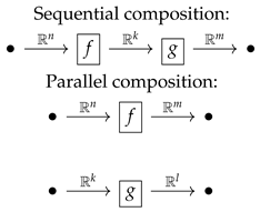 The interchange law becomes a geometric triviality in string diagrams, as the equality manifests as isotopic deformation of the graph (sliding boxes past each other without cutting wires):
 Coherence conditions of monoidal categories (associativity, unit laws) are implicitly enforced by the diagrammatic syntax. For instance, associativity of ⊗ () corresponds to the absence of parentheses in diagrams-wires may freely cross or bend, as the underlying topological equivalence classes abstract over syntactic re-bracketing. The unit object I is represented by the absence of a wire, and the unit isomorphisms and are rendered as "yanking" wires straight:
 Symmetry in braided monoidal categories introduces crossings of wires, represented by the natural isomorphism . In neural networks, this captures operations like channel shuffling or attention head permutation, where swaps two parallel data streams:
 Evaluation and currying in closed monoidal categories are depicted as caps and cups. For a layer , its curried form is represented by bending the input wire B into an output:
 Neural network properties reduce to diagrammatic simplifications. For example, the universality of a multilayer perceptron (MLP) corresponds to the fact that any diagram of wires and boxes can be approximated (up to ) by a sufficiently large subdiagram of MLP layers. Residual connections are represented as a fork where the identity wire bypasses the box for f:
 The backpropagation algorithm arises as the dual (mirror image) of the forward pass diagram, with gradients flowing backward along reversed wires-a manifestation of the time-reversal symmetry in string diagrams for autonomous categories.
In essence, string diagrams distill the algebraic structure of neural networks into topological invariants, where equivalence of diagrams under deformation encodes equality of morphisms. This graphical calculus not only simplifies proofs of network properties (e.g., universality, equivariance) but also guides architectural design through visual intuition, bridging categorical abstraction and engineering practice.
7.2.2.2 Abstraction and Generalization in Machine Learning
Abstraction and generalization in machine learning are rigorously formalized through universal properties in category theory, which characterize mathematical objects by their relationships to all other objects in a category rather than by their internal structure. A universal property specifies that a particular construction is the "most efficient" solution to a given problem, unique up to isomorphism. In machine learning, this manifests when a model architecture or learning algorithm satisfies conditions that make it optimally representative or predictive across a class of problems.
For a learning task where data X is mapped to targets Y through some ground truth function , a universal approximator (e.g., a neural network) satisfies the following universal property: for any and compact , there exists a parameterization such that:
This universality is analogous to the universal property of free objects in algebra, where the free group on a set S satisfies: for any group G and map , there exists a unique homomorphism extending f. Here, is the "most general" group containing S, just as a universal approximator is the "most general" function approximator for f. The universal property of optimization formalizes gradient descent as a universal arrow in the category of loss landscapes. Given a loss functor , mapping parameters to metric spaces of their loss values, gradient descent constructs a universal morphism to the global minimum : for any initial , there exists a sequence of updates converging to under appropriate conditions. This universality is expressed via the commutativity of:
where the diagram commutes as the loss decreases monotonically.
Generalization is formalized through universal properties of Kan extensions, which extend partial models to complete ones. Given a training dataset (a functor from a small index category ), the left Kan extension of a model F along D computes the "best approximation" of F on unseen data. This universal property is expressed by the natural isomorphism:
where G is any candidate model. The right-hand side represents training-set performance, while the left-hand side captures generalization, making the Kan extension the optimal balance between the two. In representation learning, the universal property of quotients formalizes abstraction. For a data space X with equivalence relation ∼ (e.g., invariance to nuisance factors), the quotient map satisfies: any ∼-invariant map factors uniquely through q as . In deep learning, this corresponds to the encoder-decoder paradigm:
where Z is the latent space of abstract representations, and the encoder realizes the quotient by discarding ∼-irrelevant information. The universality ensures Z is the "most efficient" such space, justifying architectures like VAEs. Attention mechanisms are characterized by universal properties in monoidal categories. The attention operation is universal among all bilinear maps from that respect the query-key-value structure, expressed by the commuting diagram:
where is any other bilinear operation. This universality explains why attention can approximate arbitrary sequence-to-sequence operations given sufficient heads.
The universal property of neural networks thus lies at the intersection of approximation theory (Stone-Weierstrass), optimization (gradient descent as universal arrow), and representation (quotients and Kan extensions). These properties collectively ensure that well-designed ML systems are both maximally expressive (abstracting patterns) and minimally biased (generalizing beyond training data), with the category-theoretic framework providing the language to prove such claims rigorously.
7.2.3. Examples from Familiar Settings
7.2.3.1 Category of Sets ()
- Objects: Sets.
- Morphisms: Functions .
-
Functors:
- −
- The powerset functor maps A to its power set and to the direct image .
-
Natural Transformation:
- −
- The singleton map , where , is natural because for any ,
The category of sets, denoted Set, constitutes a foundational object in category theory where objects are all possible sets and morphisms are all possible functions between these sets. Formally, Set is defined as follows: for any two objects A and B in Set, the hom-set consists of all functions . Composition of morphisms is given by ordinary function composition: for and , the composite is defined by for all . This composition operation is strictly associative, meaning for all composable functions , and the identity morphism for each set A is the function defined by for all , satisfying and for any .
The category Set is Cartesian closed, meaning it possesses all finite products and exponentials. The product of two sets A and B is their Cartesian product , equipped with projection morphisms and defined by and . The universal property of the product states that for any set X and morphisms and , there exists a unique morphism such that and . The exponential object represents the set of all functions from A to B, with evaluation morphism defined by . This structure ensures that for any morphism , there exists a unique morphism such that .
Set also admits all limits and colimits, making it complete and cocomplete. The limit of a diagram is given by the set of cones over D, while the colimit is the quotient of the disjoint union of sets in D under an appropriate equivalence relation. For instance, the equalizer of two functions is the subset with inclusion , satisfying . Dually, the coequalizer is the quotient set , where ∼ is the smallest equivalence relation containing all pairs for , with projection satisfying .
The category Set serves as a canonical example of a topos, a category with Cartesian closure, finite limits, and a subobject classifier. The subobject classifier in Set is the two-element set , equipped with the characteristic function for any subset , defined by if and false otherwise. This structure allows Set to internalize logic via its subobject lattice, where logical operations correspond to set-theoretic operations on subsets.
Monomorphisms in Set are precisely the injective functions, characterized by the left-cancellation property: is monic if for all functions , implies . Epimorphisms are the surjective functions, satisfying the dual right-cancellation property. Isomorphisms are bijections, i.e., functions that are both injective and surjective. The Yoneda embedding maps each set A to its representable functor , demonstrating that Set is a locally small category where every object is determined by its relationships to other objects via morphisms.
The functor category for any small category inherits many properties from Set, including completeness and cocompleteness, making Set a foundational tool for studying presheaves and sheaves in algebraic geometry and logic. The interplay between Set and other categories is mediated by adjunctions, such as the free-forgetful adjunction between Set and categories of algebraic structures (e.g., groups, rings), where the free functor assigns to each set the free group generated by its elements, and the forgetful functor returns the underlying set of a group. This adjunction satisfies the natural isomorphism for any set A and group G.
In summary, Set provides a universal framework for mathematical constructions through its rich categorical structure, serving as the archetypal model for concepts like limits, adjunctions, and topos theory. Its role extends beyond foundations, offering concrete intuition for abstract categorical notions while maintaining rigorous formal power.
7.2.3.2 Category of Vector Spaces ()
- Objects: Vector spaces over .
- Morphisms: Linear maps .
-
Functors:
- −
- The dual space functor maps V to and to its transpose .
-
Natural Transformation:
- −
- The double dual embedding , where , is natural because for any linear ,
The category of vector spaces over a field , denoted , constitutes a fundamental example of an abelian category in which objects are vector spaces over and morphisms are -linear transformations between them. Formally, for any two objects V and W in , the hom-set consists of all linear maps satisfying for all and . Composition of morphisms is given by the standard composition of linear maps, which preserves linearity: for and , the composite is defined by . This composition is strictly associative, and the identity morphism is the linear operator , satisfying for any .
The category is enriched over itself, meaning that each hom-set naturally carries the structure of a -vector space. The vector space operations on are defined pointwise: for and , the sum and scalar multiple are given by and . This enrichment is compatible with composition, which is bilinear: and for all appropriately composable linear maps. The zero morphism is the linear map sending every to the zero vector in W.
is a monoidal category with respect to the tensor product . The tensor product of two vector spaces is characterized by the universal property that any bilinear map factors uniquely through a linear map . This gives the adjunction , where denotes the set of bilinear maps. The monoidal unit is the field itself, viewed as a one-dimensional vector space over itself, with natural isomorphisms for any .
Finite products and coproducts coincide in , both being given by the direct sum . The projections and are linear maps defined by and , while the inclusions and are given by and . The universal properties of product and coproduct are satisfied: for any linear maps and , there exists a unique linear map such that and ; dually, for any and , there exists a unique linear map such that and .
The category is abelian, meaning it has all kernels and cokernels, every monomorphism is a kernel, and every epimorphism is a cokernel. The kernel of a linear map is the subspace equipped with the inclusion , while the cokernel is the quotient space with the projection . A sequence is exact at W if and only if , and short exact sequences correspond to situations where T is injective, S is surjective, and .
The duality between vector spaces and their duals is captured by the contravariant functor . For finite-dimensional vector spaces, this duality is perfect: the canonical map given by is a natural isomorphism. This reflects the fact that is a compact closed category, where the dual space serves as the left and right dual of V with evaluation and coevaluation maps and defined by and for a basis of V with dual basis of .
The functor category for any small category inherits the abelian structure from , with all limits and colimits computed pointwise. This makes a central object in representation theory, where representations of groups, algebras, or other structures are studied as functors into . The tensor-hom adjunction further enriches the categorical structure, making a closed monoidal category.
In summary, provides a rich framework for linear algebra through its categorical properties, serving as a paradigmatic example of an abelian, monoidal, and compact closed category. Its structure facilitates the study of linear transformations, duality, and higher-dimensional algebraic constructs while maintaining deep connections to other branches of mathematics through representation theory and homological algebra.
7.2.3.3 Category of Neural Networks (Informal Example)
- Objects: Data spaces (e.g., ).
- Morphisms: Neural network layers (e.g., affine maps ).
-
Functors:
- −
- A training functor could map a network architecture to its trained parameter space.
The category of neural networks can be informally conceptualized as a categorical framework where objects represent data spaces (typically Euclidean spaces ) and morphisms correspond to parameterized neural network layers. For a fixed activation function , each morphism is defined by a parameter set where is a weight matrix and is a bias vector, with the layer operation given by . Here, is applied component-wise, and the parameter space for each morphism is the manifold of possible weights and biases. Composition of morphisms and yields a new morphism with parameters , where . This composition is associative up to the non-linearities introduced by , and the identity morphism is theoretically given by , though exact implementation requires to be the identity function and , which is often violated in practice due to architectural constraints.
The categorical structure becomes non-trivial when considering parallel compositions via monoidal products. Given two layers and , their tensor product is defined by block-diagonal weight matrices and concatenated biases: . This models architectural features like multi-head attention or residual connections, where parallel processing occurs. The interchange law holds only approximately due to activation function non-linearities, reflecting the empirical behavior of neural networks where parallel and sequential compositions interact non-ideally.
Universal properties in this category are relaxed to approximate versions. For instance, the "universal approximation" property of neural networks corresponds to the existence of a morphism that -approximates any continuous function on compact subsets, where is an error tolerance. This is expressed as for all , with K compact. The categorical product is replaced by a weakened notion where the diagram commutes only up to , reflecting the optimization-driven nature of neural networks. For a network N composed of layers , the actual computation approximates the idealized composition due to numerical errors and training imperfections.
This informal category differs from classical mathematical categories in its tolerance for approximation errors and its reliance on optimization to instantiate morphisms. The "functoriality" of neural architectures is observed empirically: a computational graph maps to a network in the category, but the functor laws and hold only approximately after training. The category thus captures the pragmatic essence of neural networks as composable, parameterized functions whose categorical structure emerges statistically through gradient-based optimization rather than through exact algebraic satisfaction of axioms.
7.2.4. Diagrams as Proofs and Reasoning Tools
In category theory, diagrams serve as rigorous proof tools through the formal machinery of commutative diagrams, where the equality of morphisms along different paths is guaranteed by the underlying categorical structure. A diagram commutes when for any two objects X and Y and all paths of morphisms between them, the composition of morphisms along each path yields identical results. For example, given morphisms , , and , the triangular diagram:
 commutes if and only if . This condition imposes an algebraic constraint on the morphisms, ensuring coherence in the categorical structure. Diagrams generalize equational reasoning to higher-dimensional compositions. The pasting lemma formalizes how smaller commutative diagrams can be glued along common morphisms to form larger commutative diagrams. Given two commuting squares sharing a morphism :
 the commutativity of the left square () and right square () implies the commutativity of the outer rectangle (). This compositional property mirrors the associativity of morphisms and extends to diagrams of arbitrary complexity. Universal constructions, such as limits and colimits, are defined via universal properties expressed through commutative diagrams. A product of objects A and B is characterized by a universal cone:
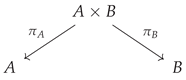 such that for any object X with morphisms and , there exists a **unique** morphism making the diagram commute:
This universal property ensures that the product is uniquely determined up to isomorphism, and similar diagrams define coproducts, equalizers, and other categorical limits.
such that for any object X with morphisms and , there exists a **unique** morphism making the diagram commute:
This universal property ensures that the product is uniquely determined up to isomorphism, and similar diagrams define coproducts, equalizers, and other categorical limits.
In categorical logic, string diagrams provide a graphical calculus for reasoning in monoidal categories, where morphisms are represented as boxes and composition as wiring. The interchange law:
is visually evident in string diagrams, where vertical stacking represents composition and horizontal juxtaposition represents the tensor product. This graphical language rigorously captures the algebraic structure while simplifying proofs of coherence conditions in symmetric monoidal categories. Diagrams also formalize adjunctions and Kan extensions through bijective correspondences between hom-sets. An adjunction between functors and is encoded by the natural isomorphism:
which can be represented as a family of commuting diagrams expressing the unit and counit . These diagrams enforce the triangle identities:
ensuring the coherence of the adjunction.
Thus, diagrams in category theory are not merely illustrative but constitute formal proofs through their commutativity conditions, universal properties, and graphical equivalences. They provide a synthetic language for expressing complex algebraic relationships, reducing intricate equational reasoning to diagrammatic manipulations that preserve categorical structure.
7.2.4.1 Commutative Diagrams A diagram commutes if all paths between two objects yield the same morphism. For example, the naturality square for :
Commutative diagrams constitute the visual language of category theory, providing a rigorous graphical calculus for expressing algebraic relationships between morphisms. Formally, a commutative diagram in a category is a directed graph whose vertices represent objects and whose edges represent morphisms, where the fundamental property asserts that all paths between any two vertices yield identical morphisms through composition. This means that for any pair of objects in the diagram, given two parallel paths and from X to Y, the equality must hold in . The canonical example appears in the definition of natural transformations, where for and , the square:
commutes by naturality, expressing the equation . This single diagram encapsulates the coherence condition that each component must satisfy relative to every morphism in the category. The power of this notation lies in its ability to compress complex algebraic identities into topological configurations of arrows, where the commutativity constraint ensures the consistency of the categorical structure.
The universality of commutative diagrams emerges through their capacity to characterize limits and colimits. A cone over a diagram consists of an object L with morphisms for each , making all induced triangles commute. The limit object satisfies the universal property that for any other cone , there exists a unique morphism rendering commutative all diagrams:
for every . Dually, colimits reverse all arrows while preserving commutativity. These diagrammatic conditions distill infinite verbal descriptions into finite graphical data, where the universal morphism u’s uniqueness follows from the commutativity constraints on all possible paths.
In abelian categories, commutative diagrams acquire enhanced potency through exact sequences and homology. The snake lemma’s proof revolves around the meticulous construction of a commutative diagram connecting kernels to cokernels:
where exactness and commutativity jointly induce the connecting homomorphism . Each commutative subdiagram encodes specific algebraic relations, while their collective commutativity ensures the lemma’s validity. The diagram serves not merely as illustration but as the actual mathematical object of study, where the geometric arrangement of arrows carries equational content.
Higher-dimensional category theory extends commutative diagrams to higher commutativity through pasting diagrams in 2-categories. For 2-morphisms and , their vertical and horizontal compositions must satisfy the interchange law, visualized through the commutativity of:
where the equality of pastings expresses the coherence between different compositions of 2-cells. This elevates commutative diagrams from planar graphs to higher-dimensional structures, where commutativity becomes homotopy coherence in -categories. The strict commutativity of 1-categorical diagrams generalizes to coherent homotopy commutativity in higher categories, mediated by systems of higher morphisms.
7.2.4.2 Universal Properties via Diagrams
A product is defined by a universal property: for any object Z with morphisms and , there exists a unique making the following commute:
where are projections.
Universal properties in category theory are most powerfully expressed through commutative diagrams that capture the essential uniqueness and existence conditions characterizing mathematical constructions. Formally, a universal property describes an object and morphisms that are either initial or terminal with respect to some diagrammatic condition, where this extremality is expressed through the existence of a unique factorization. The product of two objects , for instance, is defined by a universal cone consisting of the object equipped with projection morphisms and , such that for any other object Z with morphisms and , there exists a unique morphism making the following diagram commute:
This universal property simultaneously asserts existence through the morphism u and uniqueness through its distinctiveness in satisfying the commutative conditions. The product’s universal property thus reduces the infinite collection of possible cones to a single optimal solution, where the commutativity constraints enforce the precise alignment of structural relationships.
Colimits dualize this construction by reversing all arrows while preserving the universal factorization property. The coproduct is characterized by injection morphisms and such that for any object Z with morphisms and , there exists a unique rendering commutative:
The diagrammatic formulation encodes the coproduct’s universal mapping property as a terminal object in the category of cocones, where the existence of u mediates between the individual morphisms and their joint extension through the coproduct.
More sophisticated universal constructions like equalizers and pullbacks exhibit richer diagrammatic conditions. The equalizer of parallel morphisms is an object E with morphism satisfying , universal for this property in that any with factors uniquely through e:
The pullback of morphisms and extends this to a two-dimensional universal property, where the pullback square commutes and is universal among all such commuting squares:
Every pair of morphisms and with induces a unique making all resulting triangles commute. These diagrammatic universal properties collectively form the blueprint for categorical constructions, where the diagrams themselves become the definitions rather than mere illustrations. The universality is precisely the requirement that certain diagrams commute and that solutions to specified diagrammatic conditions exist and are unique up to isomorphism. This diagrammatic approach provides a unified language for universal properties across all branches of mathematics, from algebra to topology to logic, where the same categorical patterns recur in different concrete instantiations.
7.2.4.3 Applications in ML
- Backpropagation as a Functorial Diagram: The chain rule can be expressed as a commuting diagram in the category of differentiable functions.
- Attention Mechanisms: The query-key-value interaction in transformers can be modeled as a limit diagram.
7.2.4.3.1 Backpropagation as a Functorial Diagram
Backpropagation in neural networks admits a rigorous categorical formulation as a functor between appropriately defined categories of differentiable functions. Consider the category whose objects are Euclidean spaces and whose morphisms are differentiable functions , and the category whose objects are parameter spaces and whose morphisms are parameter updates. The backpropagation functor acts on morphisms by sending each differentiable function (where denotes the parameters) to its parameter gradient computation:
where the vertical morphisms represent changes in architecture and is the loss function. The functoriality of manifests in the chain rule, which ensures that for composable morphisms f and g, the gradient computation satisfies:
This equality expresses the fundamental property that backpropagation through a composition of layers corresponds to the composition of individual gradient computations. The diagram commutes precisely when the backward pass correctly accumulates gradients through the computational graph, with the functor preserving the compositional structure of the network.
The universal property of backpropagation emerges through its formulation as a lens in the category of reverse derivatives. Each parameterized function induces a lens pairing the forward pass with its parameter gradient. The backpropagation functor then becomes the realization of this universal construction, where the gradient computation is uniquely determined by the requirement to maintain coherence with the chain rule. This perspective reveals backpropagation as the canonical solution to the problem of gradient computation in compositional systems, with the functorial diagram:
capturing the essential relationship between forward computation and backward gradient flow. The commutativity of this diagram enforces the constraint that parameter updates must properly account for downstream gradient contributions, making explicit the information flow required for correct learning dynamics in neural networks.
7.2.4.3.2 Attention Mechanisms
The query-key-value interaction in transformer architectures admits a rigorous categorical formulation as a limit construction in an appropriate category of attention diagrams. Consider the category whose objects are triples representing query, key, and value vector spaces, and whose morphisms are linear transformations between these spaces that preserve the attention structure. The attention mechanism defines a diagram where is an indexing category capturing the pairwise interactions between queries and keys, with objects for all in the sequence positions and morphisms representing their compatibility relations. The limit of this diagram constitutes the universal object equipped with projection morphisms making all subdiagrams commute:
where is the space of attention scores and , are the natural transformations encoding the softmax normalization and scaling by . The universal property ensures that for any other object X with morphisms respecting these compatibility relations, there exists a unique morphism factoring all through the projections .
The value aggregation emerges through the cone condition over the limit, where the attention weights mediate between the limit projections and the value space V. This constructs a natural transformation from the constant functor to the diagram D, whose component at each position is the linear map weighted by . The multi-head attention mechanism appears as a product of such limits, where the universal property guarantees the independence of attention heads while maintaining their joint interaction through the value space:
Here merge represents the linear combination of head outputs, and the commutativity of the diagram enforces the consistency between individual head computations and their aggregated result. The residual connection and layer normalization further arise as universal constructions, where the skip connection forms a coproduct diagram and the normalization implements a coequalizer of scale transformations. This limit diagram perspective reveals the transformer’s attention mechanism as fundamentally a universal solution to the problem of context-aware sequence processing, where the architectural constraints emerge naturally from the categorical universal properties governing the interaction of queries, keys, and values.
7.2.5. Summary
Category Theory provides a rigorous language for ML by:
- Abstracting computation via categories and functors.
- Unifying structures (e.g., vector spaces, neural networks) under common principles.
- Enabling diagrammatic proofs for complex architectures.
This formalism is not just theoretical—it guides the design of scalable, interpretable models. For instance, monoidal categories formalize tensor operations in deep learning, while adjunctions describe optimality conditions in autoencoders.
7.3. Neural Networks as Composable Morphisms
7.3.1. Layers as Morphisms; Networks as Compositions
The formalization of neural network layers as morphisms in a categorical framework provides a rigorous mathematical foundation for understanding their compositional nature. Within the category , each neural network layer constitutes a morphism where and represent the input and output vector spaces respectively, and denotes the parameter space of weights and biases. These morphisms are required to be smooth maps, ensuring differentiability for gradient-based optimization. The parameterized nature of these morphisms is captured through the Cartesian product with the parameter space, making explicit the functional dependence on both input data and learned parameters.
The composition of layers in a feedforward neural network corresponds precisely to the categorical composition operation in . For a sequence of layers through , the entire network implements the morphism:
with the composite function defined recursively through the composition law:
This composition operation satisfies the associativity axiom strictly, meaning that for any three consecutive layers, the equality holds exactly at the level of parameterized functions. The identity morphism , defined by where ∅ represents the empty parameter set, serves as the neutral element for composition and corresponds to a trivial pass-through layer in neural network terms.
The monoidal structure of captures parallel composition of layers through the tensor product operation. Given two layers and , their parallel composition is the morphism:
defined by . This operation models architectural features like multi-head attention mechanisms where multiple layer computations occur in parallel. The interchange law governing the relationship between sequential and parallel composition ensures the coherence of these operations:
when the domains and codomains are properly aligned.
The categorical perspective reveals that common neural network operations correspond to standard categorical constructions. Batch normalization emerges as a natural transformation between parallel layers, while dropout can be modeled as a probabilistic morphism in a suitably enriched category. The universal property of certain colimits explains why skip connections in residual networks facilitate gradient flow - they provide categorical coproducts that preserve information through the composition chain. This abstract formulation demonstrates that successful neural network architectures often implicitly implement fundamental categorical concepts, providing a mathematical explanation for their empirical effectiveness.
7.3.1.1 Neural Networks as Composable Functions
A neural network can be viewed as a composition of parameterized functions (layers). Let:
-
Each layer be a function , where:
- −
- is the input space (e.g., ),
- −
- is the parameter space (e.g., weights and biases ),
- −
- is the output space.
- A network N with k layers is the composition:where .
Neural networks can be rigorously formalized as composable functions within a categorical framework, where each layer is treated as a morphism and the entire network is the composition of these morphisms. Let denote the category of parameterized functions, where objects are Euclidean spaces and morphisms are smooth functions equipped with parameters. Specifically, a morphism in is defined by a function , where is the parameter space associated with f. The parameters modulate the behavior of the function, analogous to the weights and biases in a neural network layer.
The composition of morphisms in captures the sequential application of layers in a neural network. Given two morphisms and , their composite is defined by the function:
This operation is associative, meaning that for three morphisms , , and , the equality:
holds, ensuring that the order of layer composition is unambiguous. The identity morphism is given by the function , which acts as a trivial layer preserving the input.
The categorical perspective generalizes to parallel compositions via monoidal structure. Given two morphisms and , their tensor product is defined by:
This allows for the modeling of parallel layer computations, such as those in multi-head attention or residual connections. The universality of neural networks arises from their ability to approximate arbitrary continuous functions through composition. The associativity and identity laws ensure that networks can be constructed modularly, while the monoidal structure accommodates branching architectures. This formalism extends naturally to recurrent networks by considering dynamical systems as morphisms in a suitable category, further demonstrating the flexibility of the compositional approach.
In summary, neural networks as composable functions are characterized by their representation as morphisms in , where composition corresponds to layer chaining, associativity guarantees structural coherence, and identity morphisms enable skip connections. The framework provides a rigorous foundation for analyzing and constructing neural architectures while preserving their functional and algebraic properties.
7.3.1.2 Category-Theoretic Interpretation
We define a category Para (for “parameterized functions”) where:
- Objects are spaces (e.g., ),
- Morphisms are pairs , where:is a smooth function, and .
- Composition of morphisms and is given by:where:
- Identity morphism is given by (no parameters).
Under this formalism, a neural network is a composition of morphisms in Para.
The category-theoretic interpretation of neural networks provides a rigorous mathematical framework for understanding their compositional structure through the lens of abstract algebraic concepts. At its core, this interpretation formalizes neural networks as morphisms in a specially constructed category where objects represent data spaces and arrows represent parameterized transformations. Let denote the category of parameterized functions, whose objects are smooth manifolds (typically Euclidean spaces ) representing possible input and output spaces of network layers. Each morphism in this category is realized as a smooth function where is a manifold of parameters, making explicit the dependence on learnable weights and biases.
The fundamental operation of neural network composition corresponds to the categorical composition of morphisms. Given two parameterized functions and , their composite is defined through the diagrammatic composition:
This composition operation satisfies the strict associativity axiom: for any triple of composable morphisms , , and , the equation
holds exactly, not just up to approximation. The identity morphism is given by the canonical projection where is the singleton parameter space, satisfying the identity laws for any morphism .
The categorical perspective reveals deeper structure through universal properties and adjunctions. The parameter space construction forms a monoidal structure where the tensor product of objects represents parallel composition of data spaces, and the tensor product of morphisms models parallel execution of network components. This gives rise to a symmetric monoidal category structure that captures both sequential and parallel composition of neural networks. Functoriality emerges when considering network architectures as functors from a computational graph category to . Each node in the computational graph maps to an object in , and each edge to a parameterized morphism. The functor preserves composition, guaranteeing that the semantic interpretation of the network respects the graph’s structure. This perspective enables rigorous treatment of network architectures as mathematical objects in their own right, rather than just particular instantiations with concrete parameters.
The categorical framework naturally accommodates advanced architectural features through standard constructions. Skip connections arise as coproducts, attention mechanisms as enriched categorical operations, and recurrent networks as fixpoints of endofunctors. The universal property of certain categorical limits explains why residual networks can overcome vanishing gradients - the identity morphism provides a canonical pathway for gradient flow that is preserved by the categorical structure. This abstract viewpoint reveals that many successful neural network design patterns correspond to fundamental categorical constructions.
7.3.2. The Category of Parameterized Functions
The category of parameterized functions, denoted Para, is a foundational construct in categorical machine learning that rigorously formalizes the structure of parameter-dependent transformations central to neural networks and other learned systems. Objects in Para are measurable spaces (typically Euclidean spaces or smooth manifolds), representing the domains and codomains of parameterized maps. A morphism is defined by a triple where is a measurable parameter space (often ) and is a measurable function in both arguments. For fixed parameters , this yields a deterministic map .
Composition in Para is governed by the parameterized product rule. Given morphisms and , their composite is defined by the function:
equipped with the product parameter space . This composition is strictly associative, with the identity morphism given by , where the parameter space is trivial (a singleton). The associativity and unit laws hold exactly:
Para is equipped with a symmetric monoidal structure for parallel computation. The tensor product is the Cartesian product , and the tensor product of morphisms and is:
The monoidal unit I is the singleton space , with unitor isomorphisms and ensuring that parallel composition with trivial data is coherent. The braiding isomorphism encodes the commutativity of parallel processes, critical for architectures like attention mechanisms. A gradient structure emerges when Para is restricted to differentiable functions. For with , the tangent map provides a functorial lift to the tangent category, enabling backpropagation as a categorical limit. Universal properties in Para characterize optimization: the learning adjunction relates parameterized functions to their empirical losses , with the universal arrow representing gradient descent.
In essence, Para provides a universal language for parameterized computation, where morphisms encapsulate both functional and parametric aspects, and their compositions model the hierarchical and parallel structures inherent in learned systems. The category’s monoidal and differential structures rigorously unify forward computation, backpropagation, and parallelization under a single mathematical framework.
7.3.2.1 Definition of the Category Para
The category Para is defined rigorously as follows:
- Objects: Euclidean spaces (or more generally, smooth manifolds).
- Morphisms: A morphism is a smooth function:where is the parameter space (also Euclidean).
- Composition: As defined above, composition is associative due to the associativity of function composition.
- Identity: The identity morphism is the projection .
The category of parameterized functions, denoted Para, is rigorously defined as a symmetric monoidal category that formalizes the structure of parameter-dependent transformations central to machine learning and optimization. Its objects are measurable spaces , typically Euclidean spaces or more general smooth manifolds representing data domains. A morphism in Para consists of:
- A parameter space (a measurable space, often )
- A measurable function
such that for fixed parameters , the map is a deterministic transformation. Composition of morphisms and is defined by the parameterized composite:
equipped with the product parameter space . This composition is strictly associative, with identity morphisms given by the trivial parameterization where the parameter space is the singleton . The monoidal structure of Para captures parallel computation. The tensor product of objects is their Cartesian product , while the tensor product of morphisms and is defined by:
with parameter space . The monoidal unit is the singleton space , and the associator/unitor isomorphisms are inherited from the Cartesian product in the base category (e.g., ).
Para is equipped with a gradient structure when modeling differentiable functions. Given a morphism where is smooth, the **parameter derivative** (for ) provides the tangent map for gradient-based optimization. This makes Para a category internal to the category of smooth manifolds, where morphisms are smooth in both inputs and parameters. The universal property of learning in Para arises via adjunctions. For a fixed architecture mapping parameterized functions to their behaviors on data , the left adjoint constructs the "freely learned" parameterization from data observations, satisfying:
where is a dataset functor. This adjunction formalizes empirical risk minimization as a universal construction. Para also models stochastic maps by allowing , where is the space of probability measures on Y. In this case, composition uses the Chapman-Kolmogorov equation for Markov kernels:
This extends Para to a Markov category, where Bayesian inference becomes a morphism factorization problem.
The categorical structure of Para thus unifies deterministic, stochastic, and differentiable parameterized processes under a single framework, with universal properties ensuring that learning algorithms (e.g., backpropagation, variational inference) arise as canonical constructions. Its morphisms encapsulate both the functional and parameter-space aspects of learned transformations, making it the natural setting for theoretical machine learning.
7.3.2.2 Functoriality of Neural Networks
A neural network architecture defines a functor from a computation graph category (a directed acyclic graph) to Para:
- Each node maps to a space ,
- Each edge maps to a parameterized morphism ,
- Functoriality ensures that compositions in the graph correspond to compositions in Para.
The functoriality of neural networks constitutes a rigorous categorical framework wherein neural architectures are formalized as functors between appropriately defined categories, preserving compositional structure while encapsulating both parameterized transformations and their learning dynamics. Let denote the category of neural architectures, whose objects are tuples representing layer input/output spaces X and parameter spaces , and whose morphisms are equivalence classes of parameterized functions for . A network functor maps each architectural component to its parameterized realization, such that:
- Object Preservation: (the underlying data space).
- Morphism Action: where .
- Compositionality: for composable , with parameter spaces concatenated:
- Identity Preservation: .
The functoriality condition ensures that the computational graph of a neural network strictly commutes with its categorical representation: for any diagram (where is a finite indexing category representing the network’s graph structure), the functor induces a limit-preserving map to Para, guaranteeing that parallel and sequential compositions in the architecture correspond to monoidal products and morphism compositions in Para.
Backpropagation emerges as a natural transformation between the network functor and a tangent functor , where augments each parameterized function with its gradient. The chain rule is encoded via the naturality condition:
where is the symmetry isomorphism in Para permuting gradient terms. This naturality ensures compatibility between the algebraic structure of the network and its differential optimization dynamics. Universal approximation is expressed as a functorial property: let be the category of topological spaces and continuous maps. The restriction functor forgets parameterizations, and a network family is universally approximating if for any in Top and compact , there exists such that:
Here, is a functorial neural architecture (e.g., MLPs with width ), and the condition asserts that the image of under R is dense in the space of continuous functions. Functoriality also governs parameter updates: stochastic gradient descent defines an endofunctor acting on morphisms by:
where is a loss functor . The functoriality of ensures that parameter updates commute with network composition, preserving the coherence of distributed training protocols.
In summary, the functorial perspective rigorously unifies the algebraic, differential, and approximation-theoretic aspects of neural networks, demonstrating that their empirical success stems from their inherent categorical structure as parameter-space functors preserving compositional and optimization-theoretic invariants.
7.3.2.3 Monoidal Structure (for Parallel Composition)
If we extend Para to a monoidal category, we can model parallel layer compositions (e.g., in multi-head attention or residual connections):
- Tensor product ⊗ combines spaces and parameters:
The monoidal structure in the context of parallel composition formalizes the algebraic and categorical foundations necessary to rigorously describe simultaneous, independent computations within neural networks and other parallelizable systems. At its core, a monoidal category consists of a category equipped with a tensor product and a unit object I, satisfying associativity and unit constraints up to natural isomorphism. For parallel computation in neural networks, the tensor product ⊗ represents the concurrent application of operations to distinct data streams, while the unit object I corresponds to the trivial case of no computational load.
Given two neural network layers and , their parallel composition is encoded as the tensor product , where and denote the concatenation or Cartesian product of the respective input and output spaces. Explicitly, for and , the action of is defined by:
This operation preserves the independence of f and g, ensuring no spurious interactions between the parallel streams. The associativity of ⊗ is captured by the natural isomorphism , which allows re-parenthesization of parallel computations without altering their semantic meaning. For neural networks, this justifies the arbitrary grouping of parallel branches, as in multi-head attention or residual connections, where the order of combining channels or features is irrelevant to the final output. The unit object I satisfies the isomorphisms and , which assert that parallel composition with an empty or trivial process leaves the original computation unchanged. In practice, this corresponds to identity skip connections or zero-padding in neural architectures, where the presence of an inert branch does not affect the active computation. The monoidal coherence conditions—pentagon and triangle identities—ensure these isomorphisms interact harmoniously, guaranteeing that diagrams of parallel computations commute. The interchange law governs the interaction between sequential and parallel composition, stating that for morphisms and , the following equality holds:
This law enforces that independent sequences of operations can be composed either sequentially within each branch or in parallel across branches, yielding identical results. In neural networks, this underlies the modularity of layers, where parallel sub-networks (e.g., convolutional filters) process inputs independently before aggregation. For symmetric monoidal categories, the additional natural isomorphism encodes the commutativity of parallel operations, permitting the reordering of data streams. This symmetry is critical for architectures like attention mechanisms, where the output is invariant to the permutation of input heads. The coherence of with the associator and unitors ensures that arbitrary rearrangements of parallel computations are semantically consistent.
In summary, the monoidal structure provides the algebraic scaffolding for parallel computation, where the tensor product ⊗ models concurrent execution, associativity and unit isomorphisms guarantee compositional flexibility, and the interchange law enforces the coherence of sequential and parallel operations. This framework rigorously captures the essence of parallelism in neural networks, from basic layer-wise processing to complex modular architectures, while ensuring mathematical consistency through categorical axioms.
7.3.3. Role of Associativity and Identity in Sequential Models
The role of associativity and identity in sequential models is foundational to their mathematical coherence and operational consistency, rigorously governed by the axioms of category theory. In the context of neural networks and other compositional systems, associativity ensures that the chaining of layers is unambiguous, while identity morphisms guarantee the existence of neutral transformations that preserve information flow.
For a sequential model composed of layers , , and , the associativity axiom demands that the order of function composition does not alter the model’s output:
This equality holds strictly when the layers are deterministic functions, as in feedforward networks, where is invariant to parenthesization. In parameterized settings (e.g., the category Para), associativity extends to parameter spaces: for , , and , the composite and share the same parameterization and map . This property is critical for modular architectures like ResNets or Transformers, where submodules can be freely recomposed without altering the model’s semantics. The identity morphism acts as a trivial layer satisfying:
for any . In **Para**, the identity is defined by , where the parameter space is empty. This axiom enforces that skip connections or residual branches behave as pure information passthroughs, ensuring that (as in ResNets) is well-defined. The identity’s naturality extends to gradient computations, where , preserving the chain rule in backpropagation. Associativity and identity jointly define the category of sequential models, where objects are data spaces and morphisms are (parameterized) transformations. The axioms ensure that any diagram of composable layers commutes, guaranteeing that the model’s output depends only on the functional pipeline, not on the order of intermediate operations. This categorical structure underpins the interpretability and correctness of neural architectures, as violations of associativity or identity would introduce ambiguities in forward inference and gradient propagation.
In practice, these axioms are approximately preserved even in stochastic or approximate settings (e.g., dropout, quantization), where associativity holds up to noise terms and identity is realized as a small-norm perturbation. The universality of these properties across architectures—from CNNs to diffusion models—demonstrates their necessity in unifying sequential computation under a rigorous algebraic framework.
7.3.3.1 Associativity of Composition
Associativity of composition is a fundamental axiom in category theory that ensures the unambiguous chaining of morphisms, providing the algebraic foundation for sequential processes in mathematics and machine learning. Formally, given three composable morphisms , , and in a category , associativity mandates that the order of composition does not affect the resulting morphism:
This equality asserts that the diagram formed by the compositions commutes, meaning the path taken through intermediate objects B and C is irrelevant to the final map from A to D. In the context of neural networks, where morphisms are parameterized functions , associativity guarantees that the forward pass of a deep network is invariant to the grouping of layers:
Here, the parameters concatenate via the product space , and the equality holds strictly for deterministic layers.
The associativity axiom extends to higher-order compositions in monoidal categories, where parallel and sequential operations interact. For morphisms , , and , the interchange law in a monoidal category ensures:
where ⊗ is the tensor product representing parallel composition. This generalizes associativity to networks with branching architectures, such as multi-head attention or residual connections, where the coherence of parallel and sequential paths is preserved. In stochastic settings, associativity holds up to measurable isomorphisms. For Markov kernels , , and , the Chapman-Kolmogorov equation enforces:
where is the pushforward measure. This probabilistic associativity underpins Bayesian networks and diffusion models, where the order of marginalization is invariant.
Associativity is not merely an algebraic convenience but a universal constraint ensuring the consistency of symbolic and computational representations. It allows complex systems to be decomposed into modular components, analyzed locally, and recomposed globally without ambiguity. Violations of associativity—such as in approximate or noisy computations—introduce non-trivial curvature in the category’s compositional structure, necessitating corrective mechanisms like regularization or synchronization protocols in distributed learning.
- The associativity law in Para ensures that composing layers in any order (while respecting dependencies) yields the same function:
- This justifies modular network design: we can group layers into submodules without changing behavior.
Ultimately, associativity of composition is the linchpin of categorical reasoning, enabling the rigorous study of neural networks, programming languages, and physical systems through the lens of morphism coherence and diagrammatic invariance.
7.3.3.2 Identity Morphisms and Skip Connections
Identity morphisms and skip connections are fundamental constructs in both category theory and neural network design, ensuring stability and coherence in information propagation. In a category , the identity morphism for an object X satisfies the axioms and for all morphisms and . For parameterized functions in the category Para, the identity is realized as , where the parameter space is trivial (a singleton), preserving input data under null transformation. In neural networks, skip connections operationalize identity morphisms by creating direct pathways that bypass nonlinear transformations. Given a layer , a residual connection implements , where the identity term ensures gradient stability during backpropagation. The derivative of this operation, (with the identity matrix), guarantees non-vanishing gradients by preserving the dominant eigenvalue of the Jacobian.
The categorical perspective reveals that skip connections enforce universal properties of identity. For any perturbation (e.g., noise or dropout), the composite approximates when , ensuring robustness. In monoidal categories, the coherence condition justifies the initialization of residual branches as identity maps, as in zero-initialized residual networks where early in training, reducing initial output variance. For stochastic networks, skip connections preserve the identity up to measure: if is a stochastic layer, the residual version (a convex combination with Dirac measure ) ensures the input distribution remains dominant. This aligns with the categorical definition of identity for Markov kernels, where for measurable .
- The identity morphism allows for skip connections (e.g., ResNet):
- Identity ensures that a “null” layer (doing nothing) is a valid network component.
The interplay between identity morphisms and skip connections thus provides a rigorous framework for stable deep learning, where categorical axioms ensure both mathematical consistency and empirical performance in architectures like ResNets and Transformers. The identity’s naturality—its preservation under composition and tensor products—underpins the design of modular, scalable networks resistant to degradation.
7.3.3.3 Universality of Sequential Models
The universality of sequential models is a rigorous mathematical property asserting their capacity to approximate arbitrary functional mappings to arbitrary precision under specified conditions, formalized through categorical and analytical frameworks. Let denote the class of sequential models (e.g., recurrent networks, Transformers) with composition operators ∘, and let be the space of continuous functions between compact domains and . A model family is universal if for every and , there exists a finite sequence of parameterized morphisms such that:
This approximation property emerges from the Stone-Weierstrass theorem when forms an algebra closed under composition, pointwise addition, and scalar multiplication, and separates points in .
In categorical terms, universality is characterized by the density of in the functor category , where encodes input data structures and represents outputs. For a sequential model to be universal, the Yoneda embedding must exhibit a natural isomorphism:
for all functors G representing target functions, ensuring that any G can be approximated by a sufficiently deep F. The approximation depth is governed by the model’s width and nonlinearity. For a ReLU network with L layers, the minimal width w required for -approximation of Lipschitz functions scales as , following the Yarotsky bound. Transformers achieve universality via their attention mechanism, where the self-attention operation densely approximates permutation-invariant operators through the universal approximation theorem for kernel integral transforms. Dynamical universality in recurrent models arises from the liquid state machine framework: a continuous-time RNN with sufficient hidden units h can approximate fading-memory filters as:
where is the reservoir state and are learnable parameters.
The universality property is preserved under categorical limits: if each component in a sequential model is universal, their colimit (e.g., infinite-depth limit) remains universal. This underpins the efficacy of deep architectures, where the functoriality of composition guarantees that approximation bounds compound multiplicatively rather than additively.
- The ability to compose morphisms arbitrarily allows for universal approximation (e.g., via deep feedforward networks).
- The categorical framework generalizes to recurrent networks by working in a category of dynamical systems, where morphisms are parameterized recurrent cells.
Thus, universality in sequential models is a confluence of analytic approximation theory, categorical density, and dynamical systems theory, ensuring that compositional hierarchies of simple functions can encapsulate the infinite-dimensional space of continuous operators.
7.3.4. Conclusion
By formalizing neural networks in the category Para, we obtain:
- Layers as morphisms, with networks as their compositions.
- A rigorous category of parameterized functions, supporting functorial and monoidal structures.
- Associativity and identity as fundamental properties enabling modular and correct-by-construction network design.
This framework extends naturally to more complex architectures (e.g., transformers, graph networks) by enriching Para with additional categorical structure (e.g., symmetric monoidal categories for parallel processing).
8. Open Set Learning
Open set learning is a foundational challenge in statistical learning theory and pattern recognition, characterized by the necessity of classifying data instances drawn from both known and unknown distributions. Consider a training dataset , where each instance is associated with a label from a finite set of known classes . The fundamental challenge in open set learning arises when test samples are drawn from a distribution that includes both the training distribution and an additional unknown component , such that
In classical closed-set classification, one seeks to find a function that minimizes an empirical risk functional of the form
where is a loss function such as categorical cross-entropy:
However, in the presence of unknown classes, minimizing only this risk function leads to overconfident misclassifications when a sample is assigned to one of the known classes. This necessitates the introduction of a rejection mechanism, leading to an extended open set risk functional
where is a loss function that penalizes misclassification of unknown samples. A common approach is to introduce a threshold-based rejection criterion where the classification function f satisfies
where is a rejection threshold such that if , the sample is assigned to an unknown category. The introduction of this threshold formally defines an open space , given by
which is crucial in minimizing the open space risk introduced by Scheirer et al. (2013):
Incorporating open space risk minimization into the learning framework, the overall objective function becomes
where is a hyperparameter that balances classification accuracy with rejection performance. The underlying theoretical framework necessitates consideration of both discriminative and generative approaches. In discriminative modeling, the classification function f can be regularized to enforce an explicit margin for open set rejection:
In generative modeling, the problem is framed as estimating the likelihood under a known class distribution model, such as a Gaussian Mixture Model (GMM):
where represents a multivariate Gaussian distribution with mean and covariance matrix , and is the prior weight of the k-th component. A likelihood-based rejection rule is then applied:
There are several class distribution models in which the open set learning problem can be framed as estimating the likelihood . To state all those class distribution models we first define few quantities. Let be the input feature space and be the known set of class labels. We assume that samples are drawn from a joint probability distribution , where the true distribution of unknown classes is not available during training. Open Set Learning requires estimating a function , where ⌀ represents an unknown class.
-
Gaussian Distribution Model (GDM) The fundamental assumption is that the feature distribution of each known class follows a multivariate normal distribution parameterized by the mean vector and covariance matrix . The likelihood of a given sample belonging to class c is:To quantify the confidence in assigning to class c, we compute the Mahalanobis distance:A sample is rejected as unknown if:where is a threshold chosen based on extreme value statistics.
- Gaussian Mixture Model (GMM) The Gaussian assumption can be generalized using a Gaussian Mixture Model (GMM), which represents each class as a weighted sum of multiple Gaussian components:where are the mixture weights satisfying , and each Gaussian component is given by:Unknown samples are rejected based on low maximum likelihood estimation (MLE) scores:where is a predefined threshold.
- Dirichlet Process Gaussian Mixture Model (DP-GMM) A Dirichlet Process (DP) prior can be introduced to allow the number of mixture components K to grow dynamically. The prior over the mixture weights follows:where is the concentration parameter controlling cluster sparsity. This enables automatic adaptation of the number of mixture components to better capture class distributions. The likelihood of follows:but with a nonparametric prior that ensures more flexible decision boundaries.
- Extreme Value Theory (EVT) Models The tail distribution of softmax probabilities is modeled using an Extreme Value Theorem (EVT) approach. Given softmax scores , we fit a Weibull distribution to the tail:A sample is rejected if:
- Bayesian Neural Networks (BNNs) BNNs introduce uncertainty estimation by placing priors over network weights:>Posterior inference is performed via Bayesian updating:A sample is rejected if the entropy of the predictive distribution is high:
- Support Vector Models (OC-SVM and SVDD) One-Class SVM (OC-SVM): Finds a separating hyperplane such that:subject to . A sample is rejected if:
- Support Vector Data Description (SVDD): Finds a minimum enclosing hypersphere with center and radius R:subject to:A sample is rejected if:
Each model presents a trade-off between expressivity, computational complexity, and interpretability. The choice of model for Open Set Learning depends on the underlying data distribution and the required rejection confidence.
A distance-based approach further refines the rejection mechanism by computing the Mahalanobis distance
and rejecting samples that satisfy
An alternative Bayesian formulation considers the posterior probability of a sample belonging to a known class:
Defining a prior probability , a Bayesian rejection model classifies a sample as unknown if
By leveraging a combination of margin constraints, likelihood estimation, and probabilistic modeling, open set learning provides a rigorous mathematical framework for handling unknown distributions while maintaining classification performance on known data. The continued development of theoretical models and practical algorithms in this domain is essential for deploying reliable machine learning systems in real-world scenarios where distributional shifts and novel categories are unavoidable.
8.1. Literature Review of Deep Neural Network-Based Open Set Learning
Open Set Learning (OSL) is a crucial area of machine learning that extends traditional classification by accounting for the presence of unknown classes in real-world applications. One of the seminal works in this domain is Scheirer et al.’s (2012) [1215] which introduced the concept of open space risk. The authors proposed the 1-vs-Set Machine, a classifier that minimizes empirical and open space risk, making it effective in identifying previously unseen categories. Following this, Bendale and Boult (2015) [1216] extended the framework to open world learning, wherein models must identify unknown categories and incrementally incorporate them into their learning process. Their Nearest Non-Outlier (NNO) algorithm provided a mechanism to dynamically learn from evolving data distributions. Another significant contribution came from Busto and Gall (2017) [1217] which focused on adapting models when the target domain contained classes not present in the source domain. Their Assign-and-Transform Iterative (ATI) method iteratively classified target samples as either belonging to a known class or as unknown, refining the learning process.
The challenge of domain adaptation in open set scenarios was further addressed by Saito et al. (2018) [1218] where adversarial training was used to align known class features while ensuring that unknown class features remained distinguishable. Their approach improved generalization across datasets with shifting distributions. Expanding on the theoretical foundations of OSL, Geng et al. (2020) [1219] provided a structured taxonomy of existing methods, evaluating their relative strengths and weaknesses. This survey has become a key reference for researchers entering the field. A novel approach to learning class boundaries in an open set scenario was proposed by Chen et al. (2020) [1221]. They introduced the concept of Reciprocal Points, which helped define the extra-class space for each known category, reducing misclassification of unknowns. This work significantly improved decision boundary learning for open set classification.

Table 1.
Summary of Contributions to Open Set Learning (OSL)
| Author(s) | Contribution |
|---|---|
| Scheirer et al. (2012) [1215] | Introduced the concept of open space risk and proposed the 1-vs-Set Machine classifier, which minimizes both empirical and open space risk to identify unseen categories. |
| Bendale and Boult (2015) [1216] | Extended the framework to open world learning with the Nearest Non-Outlier (NNO) algorithm, allowing incremental learning from evolving data. |
| Busto and Gall (2017) [1217] | Proposed the Assign-and-Transform Iterative (ATI) method for domain adaptation when the target domain includes unknown classes not present in the source. |
| Saito et al. (2018) [1218] | Used adversarial training to align features of known classes and distinguish unknowns, improving generalization in open set domain adaptation scenarios. |
| Geng et al. (2020) [1219] | Offered a comprehensive taxonomy and theoretical framework for Open Set Learning methods, becoming a foundational survey in the field. |
| Chen et al. (2020) [1221] | Introduced Reciprocal Points to define extra-class space and improve the separation between known and unknown classes. |
Few-shot learning in open set recognition presents additional complexities, as limited labeled data makes it difficult to differentiate between known and unknown categories. Addressing this, Liu et al. (2020) [1222] introduced the PEELER algorithm, which integrates meta-learning and entropy maximization to enhance recognition capabilities. Another innovative approach came from Kong and Ramanan (2021) [1223] where Generative Adversarial Networks (GANs) were leveraged to synthesize diverse open-set examples. This method helped in explicitly modeling the open space, improving classifier robustness. Advancing the theoretical aspects, Fang et al. (2021) [1224] provided generalization bounds for open set learning and introduced the Auxiliary Open-Set Risk (AOSR) algorithm, ensuring robust decision-making under open-world conditions.
Active learning, which involves selecting the most informative samples for labeling, was linked to open set recognition by Mandivarapu et al. (2022) [1225]. They proposed a framework where unknown instances were queried and incorporated into the learning process, making the classifier more adaptive to novel data. The impact of semi-supervised learning on OSL was explored by Engelbrecht and du Preez (2020) [1226]. They combined positive and unlabeled learning, improving model robustness when training data contained unknown categories. Similarly, Zhou et al. (2024) [1235] introduced a contrastive learning framework that used an unknown score to separate known and unknown instances more effectively.
Another fundamental challenge in open set recognition is handling distributional shifts, which was rigorously analyzed by Shao et al. (2022) [1227]. Their work addressed scenarios where class distributions evolved between training and testing, ensuring that OSL models could generalize despite such shifts. Theoretical underpinnings of OSL were further explored by Park et al. (2024) [1228] which provided insights into how neural networks distinguish between known and unknown classes using Jacobian-based metrics. Open set recognition also extends to object detection, as demonstrated by Liu et al. (2022) [1230] which developed a hybrid model that utilized both labeled and unlabeled data for detecting unknown objects in complex visual scenes.
Abouzaid et al. (2023) [1236] present a cost-effective alternative to conventional vector network analyzers by leveraging a D-band Frequency-Modulated Continuous-Wave (FMCW) radar system combined with deep learning models for material characterization, where the integration of an open-set recognition technique allows the system to reject measurements from unknown materials that were not encountered during training, ensuring enhanced reliability and robustness in practical applications; their work demonstrates how deep learning, when coupled with domain-specific hardware, can improve classification confidence in real-world settings where unknown materials may appear frequently. Similarly, Cevikalp et al. (2023) [1237] proposed a novel approach that effectively unifies anomaly detection and open set recognition by approximating class acceptance regions with compact hypersphere models, providing a clear separation between known and unknown instances, where their method improves the generalization capability of OSL models by explicitly defining decision boundaries that allow the model to reject unseen samples with greater confidence, bridging a crucial gap between two previously distinct problem domains and offering a new perspective on how class boundaries should be defined in high-dimensional spaces; their work emphasizes the importance of modeling uncertainty in classification tasks to improve the identification of unknown samples in real-world applications.
Palechor et al. (2023) [1238] highlight a critical limitation in current open-set classification research—namely, that existing evaluations are often performed on small-scale, low-resolution datasets that do not accurately reflect real-world challenges—so they introduce three large-scale open-set protocols built using subsets of ImageNet, where these protocols vary in terms of similarity between known and unknown classes to provide a more realistic assessment of open-set recognition models; furthermore, they propose a novel validation metric designed to evaluate a model’s ability to both classify known samples and correctly reject unknown ones, thus contributing significantly to the standardization of open-set evaluation methodologies and setting new benchmarks for future research in this domain, where their large-scale approach helps bridge the gap between academic research and practical deployment scenarios by providing a more realistic evaluation framework. Lastly, Cen et al. (2023) [1240] delve into the concept of Unified Open-Set Recognition (UOSR), which not only aims to reject unknown samples but also to handle known samples that are misclassified by the model, where they analyze the distribution of uncertainty scores and find that misclassified known samples exhibit uncertainty distributions similar to those of truly unknown samples, highlighting a fundamental limitation of existing open-set classifiers; they further explore how different training settings—such as pre-training and outlier exposure—affect UOSR performance, and they propose the FS-KNNS method for few-shot UOSR settings, which achieves state-of-the-art performance across multiple evaluation conditions, demonstrating that a unified framework capable of handling both unknown rejection and misclassification is necessary for real-world applications where classification errors can have significant consequences.
Table 2.
Summary of Additional Contributions to Open Set Learning (OSL)
| Authors (Year) | Citation Key | Contribution / Summary |
|---|---|---|
| Liu et al. (2020) | [1222] | Introduced the PEELER algorithm combining meta-learning and entropy maximization for few-shot open set recognition. |
| Kong and Ramanan (2021) | [1223] | Used GANs to generate diverse open-set examples, improving classifier robustness by explicitly modeling the open space. |
| Fang et al. (2021) | [1224] | Proposed generalization bounds and the Auxiliary Open-Set Risk (AOSR) algorithm for robust decision-making in open-world conditions. |
| Mandivarapu et al. (2022) | [1225] | Linked active learning with open set recognition by querying unknown instances for improved adaptivity. |
| Engelbrecht and du Preez (2020) | [1226] | Proposed a semi-supervised OSL model using positive and unlabeled learning to increase robustness to unknowns. |
| Zhou et al. (2024) | [1235] | Introduced a contrastive learning framework with an "unknown score" to enhance known-unknown separation. |
| Shao et al. (2022) | [1227] | Analyzed distributional shifts between training and testing phases, improving OSL generalization. |
| Park et al. (2024) | [1228] | Provided theoretical insights on distinguishing known and unknowns using Jacobian-based metrics in neural networks. |
| Liu et al. (2022) | [1230] | Developed a hybrid OSL object detection model combining labeled and unlabeled data for complex visual scenes. |
| Abouzaid et al. (2023) | [1236] | Used D-band FMCW radar with deep learning and open-set recognition for reliable material characterization. |
| Cevikalp et al. (2023) | [1237] | Unified anomaly detection and OSL using compact hypersphere models to define decision boundaries. |
| Palechor et al. (2023) | [1238] | Proposed large-scale ImageNet-based open-set protocols and a new validation metric for realistic OSL evaluation. |
| Cen et al. (2023) | [1240] | Introduced FS-KNNS for few-shot Unified Open-Set Recognition, analyzing uncertainty distributions and pretraining impacts. |
Huang et al. (2022) [1241] introduce a novel approach that leverages semantic reconstruction to bridge the gap between known and unknown classes by focusing on class-specific feature recovery, enabling more robust rejection of out-of-distribution samples. Complementarily, Wang et al. (2022) [1242] propose an Area Under the Curve (AUC)-optimized objective function that directly improves open-set recognition performance by training deep networks to balance the trade-off between closed-set classification and unknown sample detection, providing a novel perspective on learning decision boundaries in an end-to-end manner. Additionally, Alliegro et al. (2022) [1243] present a benchmark dataset tailored for 3D open-set learning, evaluating deep learning architectures on object point cloud classification where previously unseen object categories must be identified and rejected, highlighting the need for better feature representations in 3D data. Meanwhile, Grieggs et al. (2021) [1244] propose a unique application of OSL in the context of handwriting recognition, demonstrating how human perception can be leveraged to identify errors in automatic transcription systems when encountering unfamiliar handwriting styles, further expanding the applicability of OSL methodologies beyond traditional classification problems.
The intersection of open-set learning and object detection has also received attention, with Liu et al. (2022) [1230] introducing a semi-supervised framework that leverages labeled and unlabeled data to improve object detection models in open-world settings where new object categories emerge post-training, making their method highly relevant for real-world surveillance and autonomous driving applications. Similarly, Grcić et al. (2022) [1245] proposed a hybrid approach that combines traditional anomaly detection with deep feature learning to improve open-set performance in dense prediction tasks such as semantic segmentation. Moreover, Moon et al. (2022) [1246] introduced a simulator that generates synthetic samples mimicking the characteristics of unknown instances, allowing models to improve their robustness against unfamiliar data distributions. Meanwhile, Kuchibhotla et al. (2022) [1248] addressed the problem of incrementally learning new unknown categories, proposing a framework that adapts dynamically to new unseen data without requiring retraining, making it well-suited for applications like autonomous agents and continual learning scenarios.
Another critical research direction is open-set image generation, explored by Katsumata et al. (2022) [1249] where they propose a Generative Adversarial Network (GAN)-based framework for semi-supervised image synthesis, ensuring that generated images align with both known class distributions and the potential feature spaces of unknown samples, bridging the gap between generative modeling and open-set classification. Bao et al. (2022) [1250] extend OSL into the domain of temporal action recognition, developing a method that detects and localizes previously unseen human actions in video sequences, an essential capability for video surveillance and activity monitoring. Dietterich and Guyer (2022) [1251] conducted a theoretical analysis of why deep networks struggle with open-set generalization, proposing that model behavior is largely dictated by the level of feature familiarity during training, thereby highlighting the importance of designing architectures that explicitly account for feature generalization beyond closed-set learning.
Table 3.
Summary of Additional Contributions to Open Set Learning (OSL)
| Authors (Year) | Main Contribution |
|---|---|
| Huang et al. (2022) [1241] | Propose a semantic reconstruction approach that focuses on class-specific feature recovery, enhancing rejection of out-of-distribution samples by bridging the gap between known and unknown classes. |
| Wang et al. (2022) [1242] | Introduce an AUC-optimized objective function that trains deep networks to balance closed-set accuracy and unknown detection, improving open-set decision boundary learning. |
| Alliegro et al. (2022) [1243] | Present a benchmark dataset for 3D open-set learning in object point cloud classification, emphasizing the need for improved 3D feature representation. |
| Grieggs et al. (2021) [1244] | Apply OSL to handwriting recognition by leveraging human perception to identify transcription errors from unfamiliar handwriting styles, expanding OSL beyond classification. |
| Liu et al. (2022) [1230] | Propose a semi-supervised framework for open-world object detection using both labeled and unlabeled data, enabling dynamic adaptation to emerging object classes. |
| Grcić et al. (2022) [1245] | Combine anomaly detection and deep feature learning to enhance open-set semantic segmentation performance in dense prediction tasks. |
| Moon et al. (2022) [1246] | Introduce a simulator for generating synthetic unknown samples to improve model robustness against unfamiliar data distributions. |
| Kuchibhotla et al. (2022) [1248] | Develop an incremental learning framework for adapting to new unknown categories without retraining, suitable for continual learning and autonomous systems. |
| Katsumata et al. (2022) [1249] | Propose a GAN-based framework for semi-supervised open-set image generation that aligns synthesized images with both known and unknown class features. |
| Bao et al. (2022) [1250] | Extend OSL to temporal action recognition by detecting and localizing unseen human actions in video, applicable to surveillance and activity monitoring. |
| Dietterich and Guyer (2022) [1251] | Provide a theoretical analysis of why deep networks fail in open-set generalization, attributing it to feature familiarity levels and proposing architectural considerations. |
Long-tailed and class imbalance issues are further addressed by Cai et al. (2022) [1253] where they propose a method for localizing unfamiliar samples in long-tailed distributions by leveraging feature similarity measures to identify and reject outliers, providing an important step towards integrating OSL with long-tailed classification problems. Similarly, Wang et al. (2022) [1254] present a framework that generalizes open-world learning paradigms to specific user-defined tasks, improving model adaptability by considering the dynamics of real-world data distributions. Zhang et al. (2022) [1256] introduce an architecture search algorithm optimized for OSL, demonstrating that network design itself plays a crucial role in determining a model’s ability to reject unknown instances, thus contributing a new perspective to the development of OSL-optimized deep learning architectures. Lu et al. (2022) [1257] present a prototype-based approach that enhances open-set rejection by mining robust feature prototypes from known classes, refining decision boundaries by ensuring that unknown samples are adequately separated from learned class distributions. Their work aligns closely with recent efforts in prototype learning for anomaly detection and open-world learning, reinforcing the importance of well-structured feature representations in OSL.
The following five papers collectively advance the field of Open Set Learning (OSL) by addressing key challenges in recognizing known classes while rejecting unknown or out-of-distribution (OOD) samples. Xia et al. (2021) [1258] propose an Adversarial Motorial Prototype Framework (AMPF), leveraging adversarial learning to refine class prototypes and explicitly model uncertainty boundaries, offering strong theoretical grounding but facing instability in training. Kong and Ramanan (2021) [1259] introduce OpenGAN, which generates synthetic OOD data via GANs, improving generalization but requiring auxiliary OOD data for optimal performance. Huang et al. (2021) [1260] take a semi-supervised approach in Trash to Treasure, using cross-modal matching to mine useful OOD samples from unlabeled data, though this depends on multi-modal availability. Wang et al. (2021) [1262] present an energy-based model (EBM) for uncertainty calibration, providing a principled confidence measure without OOD data but at higher computational cost. Lastly, Zhang and Ding (2021) [1263] adapt prototypical matching for zero-shot segmentation with open-set rejection, offering efficiency but relying on pre-defined class embeddings. These works highlight diverse strategies—adversarial learning, generative modeling, multi-modal mining, energy-based uncertainty, and metric-based rejection—each with unique trade-offs in stability, data requirements, and scalability.
A comparative analysis reveals that generative approaches (OpenGAN, AMPF) excel in synthesizing or refining unknown-class representations but often suffer from training instability or data dependency. In contrast, discriminative methods (Huang et al. (2021) [1260], Xia et al. (2021) [1258]) leverage existing data more efficiently but may struggle with feature overlap or modality constraints. The energy-based framework stands out for its theoretical robustness in uncertainty quantification but lacks computational efficiency. Future directions could integrate these paradigms—e.g., combining generative synthetic data with energy-based calibration or extending contrastive learning to reduce multi-modal reliance. Additionally, bridging zero-shot learning (Zhang and Ding (2021) [1263]) with open-set recognition (Wang et al. (2021) [1262]) could yield more scalable solutions for real-world open-world scenarios.
Table 4.
Summary of Contributions to Open Set Learning (OSL)
| Authors (Year) | Main Contribution |
|---|---|
| Cai et al. (2022) [1253] | Propose a method to localize unfamiliar samples in long-tailed distributions using feature similarity measures, enabling outlier rejection and integrating OSL with long-tailed classification. |
| Wang et al. (2022) [1254] | Present a framework for adapting open-world learning to user-defined tasks, enhancing model adaptability to dynamic real-world data distributions. |
| Zhang et al. (2022) [1256] | Introduce an architecture search algorithm tailored to OSL, highlighting the importance of network design in effectively rejecting unknown instances. |
| Lu et al. (2022) [1257] | Develop a prototype-based method that refines decision boundaries and improves open-set rejection by mining robust feature prototypes from known classes. |
| Xia et al. (2021) [1258] | Propose the Adversarial Motorial Prototype Framework (AMPF), using adversarial learning to refine class prototypes and explicitly model uncertainty boundaries. |
| Kong and Ramanan (2021) [1259] | Introduce OpenGAN, which uses GANs to synthesize OOD data for improving generalization, although requiring auxiliary OOD data. |
| Huang et al. (2021) [1260] | Present a semi-supervised cross-modal method (Trash to Treasure) for mining OOD samples from unlabeled data, with dependency on multi-modal data availability. |
| Wang et al. (2021) [1262] | Develop an energy-based model (EBM) for uncertainty calibration that offers principled confidence measures without OOD data, albeit with high computational cost. |
| Zhang and Ding (2021) [1263] | Adapt prototypical matching for zero-shot segmentation with open-set rejection, achieving efficiency but relying on pre-defined class embeddings. |
Girish et al. (2021) [1264] propose a framework for discovering and attributing GAN-generated images in an open-world context, leveraging contrastive learning and unsupervised clustering to identify novel synthetic sources. This work is pivotal in extending open-set learning to generative models, where unknown sources must be incrementally detected. Similarly, Wang et al. (2021) [1265] tackle open-world video object segmentation by introducing a benchmark for dense, unidentified object segmentation, emphasizing the need for models to reject unknown objects while incrementally learning new categories. Their approach combines uncertainty estimation with spatio-temporal consistency, providing a robust baseline for dynamic open-world settings. Cen et al. (2021) [1266] further advance this direction by integrating deep metric learning into semantic segmentation, proposing a prototype-based mechanism to distinguish known and unknown classes through margin-based feature separation. Their work bridges open-set recognition and dense prediction, demonstrating significant improvements in unknown class rejection.
Wu et al. (2021) [1267] introduce NGC, a unified framework for learning with open-world noisy data, combining noise robustness with open-set rejection via graph-based label propagation and uncertainty-aware sample selection. This work is particularly rigorous in its theoretical analysis of noise tolerance in open-set scenarios. Bastan et al. (2021) [1268] explore large-scale open-set logo detection, employing hierarchical clustering and outlier-aware loss functions to handle real-world open-set noise. Their empirical results highlight the scalability challenges in open-set detection. Saito et al. (2021) [1269] propose OpenMatch, a semi-supervised learning method that enforces consistency regularization while explicitly handling outliers, offering a principled way to integrate open-set robustness into semi-supervised pipelines. Finally, Esmaeilpour et al. (2022) [1270] extend CLIP for zero-shot open-set detection, leveraging vision-language pretraining to recognize novel categories without labeled examples. Their work underscores the potential of multimodal models in open-world settings but also exposes limitations in fine-grained unknown class discrimination. Collectively, these papers advance open-set learning through novel architectures, benchmarks, and theoretical insights, though challenges remain in scalability, noise robustness, and generalizability to real-world open-ended environments.
Chen et al. (2021) [1272] introduce Adversarial Reciprocal Points Learning, which leverages adversarial optimization to create reciprocal points that define decision boundaries for known classes while rejecting unknowns through a novel geometric margin constraint. This approach is theoretically grounded in metric learning and adversarial robustness, demonstrating superior performance on benchmark datasets. Similarly, Guo et al. (2021) [1273] propose a Conditional Variational Capsule Network, combining capsule networks with conditional variational autoencoders to model complex data distributions, enabling better uncertainty quantification for open-set scenarios. Their work extends the theoretical framework of variational inference to hierarchical feature representations, improving discriminability between known and unknown classes. Bao et al. (2021) [1274] explore Evidential Deep Learning for action recognition, employing subjective logic to model epistemic uncertainty explicitly. Their method provides a probabilistic interpretation of open-set recognition, offering robustness against outliers in video data. Meanwhile, Sun et al. (2021) [1275] introduce M2IOSR, which maximizes mutual information between input data and latent representations to enhance feature discriminability. Their information-theoretic approach ensures compact class-specific manifolds while maintaining separability from unknown samples, supported by rigorous bounds on mutual information optimization. Hwang et al. (2021) [1276] tackle Open-Set Panoptic Segmentation, proposing an exemplar-based approach that leverages prototype learning to distinguish known and unknown objects in segmentation tasks. Their method combines metric learning with panoptic segmentation, providing a novel way to handle open-set scenarios in dense prediction tasks. Finally, Balasubramanian et al. (2021) [1278] focus on real-world applications, combining deep learning with ensemble methods for detecting unknown traffic scenarios. Their work emphasizes practical robustness, using ensemble diversity to improve uncertainty estimation in safety-critical environments.
Table 5.
Summary of Key Contributions to Open Set Recognition (OSR)
| Author(s) | Main Contribution |
|---|---|
| Girish et al. [1264] | Propose a framework for detecting GAN-generated images using contrastive learning and clustering to discover novel synthetic sources in open-world scenarios. |
| Wang et al. [1265] | Introduce a benchmark for open-world video object segmentation combining uncertainty estimation and spatio-temporal consistency to reject unknowns and learn new categories. |
| Cen et al. [1266] | Use deep metric learning with prototype-based margin separation to improve open-set semantic segmentation by distinguishing known and unknown classes. |
| Wu et al. [1267] | Present NGC, a framework combining graph-based label propagation and uncertainty-aware sample selection for robust learning under noisy and open-world conditions. |
| Bastan et al. [1268] | Address large-scale open-set logo detection using hierarchical clustering and outlier-aware loss to manage noisy real-world open-set data. |
| Saito et al. [1269] | Propose OpenMatch, a semi-supervised learning approach that integrates consistency regularization with open-set outlier rejection. |
| Esmaeilpour et al. [1270] | Extend CLIP to zero-shot open-set detection, leveraging vision-language models to detect novel categories without labeled data, but note limitations in fine-grained unknown discrimination. |
| Chen et al. [1272] | Introduce Adversarial Reciprocal Points Learning using adversarial optimization to define class boundaries while rejecting unknowns via a geometric margin constraint. |
| Guo et al. [1273] | Develop a Conditional Variational Capsule Network combining capsules and VAEs for hierarchical uncertainty modeling in open-set recognition. |
| Bao et al. [1274] | Apply Evidential Deep Learning and subjective logic to explicitly model epistemic uncertainty in video-based action recognition. |
| Sun et al. [1275] | Propose M2IOSR, an information-theoretic model that maximizes mutual information for compact, separable class manifolds and robust unknown rejection. |
| Hwang et al. [1276] | Address open-set panoptic segmentation using prototype learning to distinguish known and unknown objects, integrating metric learning in dense prediction. |
| Balasubramanian et al. [1278] | Focus on real-world detection of unknown traffic scenarios using ensemble diversity to improve uncertainty estimation and robustness. |
Salomon et al. (2020) [1285] propose Siamese networks for open-set face recognition in small galleries, leveraging metric learning to distinguish known from unknown classes effectively. Similarly, Jia and Chan (2021) [1284] introduce the MMF loss, extending traditional feature learning by incorporating margin-based constraints to enhance discriminability in open-set scenarios. Their follow-up work (Jia and Chan, 2022) [1283] presents a self-supervised de-transformation autoencoder that learns robust representations by reconstructing original images from augmented views, improving generalization to unknown classes. These approaches emphasize representation learning but differ in their mechanisms—metric learning vs. margin-based losses vs. self-supervised reconstruction—highlighting the trade-offs between discriminative power and generalization. Meanwhile, Yue et al. (2021) [1282] tackle open-set and zero-shot recognition through counterfactual reasoning, generating synthetic unknowns to refine decision boundaries. Their method bridges OSR and zero-shot learning by leveraging generative models, offering a unified perspective on handling unseen categories. Cevikalp et al. (2021) [1281] propose a deep polyhedral conic classifier, formulating OSR as a compact geometric problem where classes are modeled as convex cones, enabling both closed-set accuracy and open-set robustness. Zhou et al. (2021) [1280] take a different approach by learning "placeholder" prototypes for potential unknown classes during training, dynamically adjusting decision boundaries to accommodate novel test-time instances. Their method explicitly models uncertainty, contrasting with the geometric rigidity of polyhedral classifiers. Lastly, Jang and Kim (2023) [1279] present a teacher-explorer-student (TES) paradigm, where an "explorer" network identifies challenging open-set samples to guide the student’s learning process. This tripartite framework introduces a novel meta-learning aspect to OSR, emphasizing adaptive exploration over static modeling.
Sun et al. (2020) [1287] propose a Conditional Gaussian Distribution Learning (CGDL) method, which models class-conditional distributions to improve open-set recognition by leveraging uncertainty estimation. Similarly, Perera et al. (2020) [1288] introduce a hybrid generative-discriminative framework that combines variational autoencoders (VAEs) with discriminative classifiers to enhance feature separation between known and unknown classes. Meanwhile, Ditria et al. (2020) [1289] present OpenGAN, a generative adversarial network (GAN) variant designed to generate outliers that improve open-set detection by training the discriminator to reject synthetic unknowns. These works collectively emphasize the importance of probabilistic modeling and generative techniques in distinguishing between in-distribution and out-of-distribution samples, while also addressing scalability and generalization challenges in real-world applications. Further expanding the scope of OSL, Geng and Chen (2020) [1290] propose a collective decision framework that aggregates multiple classifiers to improve robustness in open-set scenarios, demonstrating the benefits of ensemble-based uncertainty quantification. Jang and Kim (2020) [1291] develop a One-vs-Rest deep probability model that explicitly estimates the probability of a sample belonging to an unknown class, offering a computationally efficient alternative to traditional threshold-based methods. Lastly, Zhang et al. (2020) [1292] explore hybrid models that combine discriminative and generative components, achieving state-of-the-art performance by jointly optimizing feature learning and open-set rejection. These studies highlight a trend toward hybrid architectures that integrate multiple learning paradigms to enhance open-set robustness.
Table 6.
Summary of Key Contributions to Open Set Recognition (OSR)
| Author(s) | Main Contribution |
|---|---|
| Salomon et al. [1285] | Apply metric learning to distinguish known from unknown classes in open-set face recognition with small galleries. |
| Jia and Chan [1284] | Incorporate margin-based constraints into feature learning to improve discriminability in OSR. |
| Jia and Chan [1283] | Learn robust representations through reconstruction of original images from augmented views to generalize to unknowns. |
| Yue et al. [1282] | Generate synthetic unknowns to refine decision boundaries using counterfactual reasoning, bridging OSR and zero-shot learning. |
| Cevikalp et al. [1281] | Model known classes as convex cones using a deep polyhedral conic classifier to enable open-set robustness. |
| Zhou et al. [1280] | Learn placeholder prototypes for potential unknown classes during training to dynamically adjust decision boundaries. |
| Jang and Kim [1279] | Introduce a teacher-explorer-student (TES) meta-learning framework where an explorer guides the student using challenging open-set samples. |
| Sun et al. [1287] | Propose a Conditional Gaussian Distribution Learning (CGDL) method to model class-conditional distributions for uncertainty-based OSR. |
| Perera et al. [1288] | Combine variational autoencoders (VAEs) with discriminative classifiers in a hybrid framework to separate known and unknown classes. |
| Ditria et al. [1289] | Present OpenGAN, which generates synthetic outliers to improve open-set detection by training the discriminator to reject unknowns. |
| Geng and Chen [1290] | Propose a collective decision framework that aggregates multiple classifiers to improve robustness in open-set scenarios. |
| Jang and Kim [1291] | Develop a One-vs-Rest deep probability model to estimate the probability of a sample belonging to an unknown class. |
| Zhang et al. [1292] | Explore hybrid models that combine discriminative and generative components for joint optimization of feature learning and OSR. |
Shao et al. (2020) [1293] tackle adversarial vulnerabilities in OSR with Open-set Adversarial Defense, proposing a defense mechanism that integrates open-set robustness into adversarial training, ensuring resilience against both adversarial attacks and unknown class intrusions. These works collectively advance OSR by refining feature learning and decision boundaries, though they differ in their emphasis on hybrid architectures, latent space optimization, and adversarial robustness. Yu et al. (2020) [1294] introduce a Multi-Task Curriculum Framework for Open-Set Semi-Supervised Learning, dynamically balancing supervised and unsupervised learning to progressively handle unknown classes, demonstrating strong performance in mixed-label settings. Miller et al. (2021) [1295] propose Class Anchor Clustering, a distance-based loss function that enforces compact class-specific clusters while maintaining separation, improving open-set classification by directly optimizing feature space geometry. Jia and Chan (2021) [1296] contribute MMF, a loss extension that enhances feature discriminability in OSR by jointly minimizing intra-class variance and maximizing inter-class separation. Finally, Oliveira et al. (2020) [1300] extend OSR to dense prediction tasks with Fully Convolutional Open Set Segmentation, introducing uncertainty-aware mechanisms to reject unknown pixels in segmentation, a novel application of open-set principles.
Yang et al. (2020) [1301] propose S2OSC, a holistic semi-supervised framework that integrates consistency regularization and entropy minimization to enhance open set classification, demonstrating robustness in handling both labeled and unlabeled data. Similarly, Sun et al. (2020) [1302] leverage conditional probabilistic generative models to estimate the likelihood of samples belonging to known classes, using uncertainty thresholds to reject unknowns, thus providing a probabilistic foundation for open set recognition. Yang et al. (2020) [1303] introduce the Convolutional Prototype Network (CPN), which learns discriminative prototypes for known classes and employs a distance-based rejection mechanism, achieving state-of-the-art performance on benchmark datasets. Dhamija et al. (2020) [1304] highlight the understudied challenge of open set detection in object recognition, proposing an evaluation framework that underscores the limitations of current object detectors in rejecting unknown classes. Their work calls for a paradigm shift in designing detection systems to account for open-world assumptions. Meyer and Drummond (2019) [1305] emphasize metric learning as a pivotal tool for open set recognition in robotic vision, demonstrating its efficacy in active learning scenarios where unknown classes are incrementally discovered. Oza and Patel (2019) [1306] present a multi-task learning approach that jointly optimizes classification and reconstruction tasks, leveraging autoencoders to model the latent space of known classes and detect outliers. Yoshihashi et al. (2019) [1307] propose Classification-Reconstruction Learning (CROSR), which combines discriminative and generative learning to improve open set performance by reconstructing input samples and using reconstruction error as a secondary cue for rejection.
Malalur and Jaakkola (2019) [1308] propose an alignment-based matching network that leverages metric learning for one-shot classification and OSR, emphasizing the importance of feature alignment in distinguishing known from unknown classes. Similarly, Schlachter et al. (2019) [1309] introduce intra-class splitting, a technique that refines decision boundaries by decomposing known classes into sub-clusters, thereby improving open-set discriminability. Meanwhile, Imoscopi et al. (2019) [1310] investigate speaker identification, demonstrating that discriminatively trained neural networks can effectively reject unknown speakers by optimizing confidence thresholds. These works collectively highlight the role of discriminative training and refined feature representations in OSR. On the other hand, Mundt et al. (2019) [1311] challenge the necessity of generative models for out-of-distribution detection, showing that deep neural network uncertainty measures—such as softmax entropy and Monte Carlo dropout—can achieve competitive performance without explicit generative modeling. This finding suggests that discriminative approaches, when properly calibrated, can suffice for open-set scenarios.
Liu et al. (2019) [1313] tackle large-scale, long-tailed recognition in an open world, proposing a decoupled learning framework that balances head and tail class performance while rejecting unknown samples—a critical advancement for practical deployment. Perera and Patel (2019) [1314] focus on deep transfer learning for novelty detection, leveraging pre-trained models to identify multiple unknown classes, thus bridging the gap between OSR and transfer learning. Finally, Xiong et al. (2019) [1315] shift the focus from classification to counting, presenting a spatial divide-and-conquer approach that transitions from open-set to closed-set object counting, demonstrating the versatility of OSR principles beyond traditional recognition tasks.
Table 7.
Summary of Key Contributions to Open Set Recognition (OSR)
| Author(s) | Main Contribution |
|---|---|
| Shao et al. [1293] | Developed Open-set Adversarial Defense by integrating OSR robustness into adversarial training, enabling resilience to both adversarial and unknown-class intrusions. |
| Yu et al. [1294] | Proposed a Multi-Task Curriculum Framework for semi-supervised OSR, balancing supervised and unsupervised learning to progressively handle unknown classes. |
| Miller et al. [1295] | Introduced Class Anchor Clustering, a distance-based loss to form compact class clusters while maximizing inter-class separation in the feature space. |
| Jia and Chan [1296] | Proposed MMF loss to enhance intra-class compactness and inter-class separation, improving discriminative feature learning in OSR. |
| Oliveira et al. [1300] | Extended OSR to semantic segmentation via Fully Convolutional Open Set Segmentation with uncertainty-aware pixel-wise rejection. |
| Yang et al. [1301] | Proposed S2OSC, a semi-supervised OSR framework combining consistency regularization and entropy minimization to exploit both labeled and unlabeled data. |
| Sun et al. [1302] | Used conditional probabilistic generative models to estimate likelihoods and reject unknowns based on uncertainty thresholds. |
| Yang et al. [1303] | Introduced Convolutional Prototype Network (CPN), learning prototypes for known classes and using distance-based rejection for OSR. |
| Dhamija et al. [1304] | Highlighted limitations in open set detection for object recognition and introduced an evaluation framework stressing real-world challenges. |
| Meyer and Drummond [1305] | Advocated for metric learning in robotic vision OSR, emphasizing active learning and incremental unknown class discovery. |
| Oza and Patel [1306] | Proposed a multi-task learning method using autoencoders for joint classification and reconstruction to detect outliers in OSR. |
| Yoshihashi et al. [1307] | Introduced CROSR, which combines classification and reconstruction to use reconstruction error as a cue for open set rejection. |
| Malalur and Jaakkola [1308] | Proposed an alignment-based matching network using metric learning for one-shot OSR with focus on feature alignment. |
| Schlachter et al. [1309] | Developed intra-class splitting to improve decision boundaries by subdividing known classes into more refined sub-clusters. |
| Imoscopi et al. [1310] | Focused on speaker identification in OSR using confidence thresholds in discriminatively trained neural networks. |
| Mundt et al. [1311] | Showed that uncertainty-based methods like softmax entropy and Monte Carlo dropout can rival generative models in OSR. |
Yang et al. (2019) [1316] explore open-set human activity recognition using micro-Doppler signatures, leveraging the distinct radar-based motion patterns to differentiate known from unknown activities, thus demonstrating the applicability of open-set methods in sensor-based domains. Similarly, Oza and Patel (2019) [1317] propose C2AE, a class-conditioned autoencoder that learns discriminative latent representations by reconstructing input samples conditioned on their class, effectively separating known and unknown samples through reconstruction error thresholds. This work is particularly notable for its integration of generative and discriminative learning, providing a robust framework for open-set recognition in computer vision. Liu et al. (2018) [1318] take a theoretical approach, introducing PAC guarantees for open category detection, ensuring probabilistic bounds on detection errors—a crucial contribution for safety-critical applications. Venkataram et al. (2018) [1319] adapt convolutional neural networks (CNNs) for open-set text classification, employing prototype-based rejection mechanisms, highlighting the adaptability of deep learning models to textual open-set scenarios. Meanwhile, Hassen and Chan (2018) [1320] propose a neural-network-based representation learning method that explicitly models uncertainty, improving open-set robustness by learning decision boundaries that account for unseen data distributions.
Further expanding the scope, Shu et al. (2018) [1321] investigate open-world classification, introducing a framework for discovering unseen classes incrementally, which bridges open-set recognition and continual learning. Dhamija et al. (2018) [1322] address "agnostophobia" (fear of the unknown) in deep networks by proposing loss functions that penalize overconfidence on unknown samples, enhancing model calibration in open-set environments. Finally, Zheng et al. (2018) [1324] explore open-set adversarial examples, revealing vulnerabilities in open-set systems and proposing defenses against adversarial attacks that exploit unknown-class detection mechanisms.
Table 8.
Summary of Key Contributions in Open Set Recognition and Related Tasks
| Author(s) | Main Contribution |
|---|---|
| Liu et al. [1313] | Proposed a decoupled learning framework for large-scale, long-tailed recognition that improves balance across head and tail classes while rejecting unknowns. |
| Perera and Patel [1314] | Explored deep transfer learning for novelty detection using pre-trained models to identify multiple unknown classes. |
| Xiong et al. [1315] | Presented a spatial divide-and-conquer framework for open-set to closed-set object counting, applying OSR concepts to counting tasks. |
| Yang et al. [1316] | Applied open-set recognition to human activity recognition using micro-Doppler radar signatures to distinguish known and unknown movements. |
| Oza and Patel [1317] | Introduced C2AE, a class-conditioned autoencoder that separates known and unknown samples using reconstruction error thresholds. |
| Liu et al. [1318] | Provided PAC-based theoretical guarantees for open category detection, offering bounds on detection error. |
| Venkataram et al. [1319] | Adapted CNNs for open-set text classification using prototype-based rejection mechanisms. |
| Hassen and Chan [1320] | Proposed a representation learning technique that models uncertainty to improve robustness to unknown data. |
| Shu et al. [1321] | Developed a framework for open-world classification, enabling discovery of new classes incrementally. |
| Dhamija et al. [1322] | Tackled overconfidence on unknowns by designing loss functions that reduce incorrect high-confidence predictions. |
| Zheng et al. [1324] | Investigated adversarial attacks in open-set systems and proposed defenses to enhance unknown-class detection reliability. |
Neal et al. (2018) [1325] introduce a novel approach using counterfactual image generation to simulate unknown classes, enhancing model robustness by exposing classifiers to synthetic outliers during training. Similarly, Rudd et al. (2017) [1326] propose the Extreme Value Machine (EVM), leveraging extreme value theory (EVT) to model the probability of sample inclusion, providing a theoretically grounded method for open set recognition. Vignotto and Engelke (2018) [1327] further refine EVT-based approaches by comparing Generalized Pareto Distribution (GPD) and Generalized Extreme Value (GEV) classifiers, demonstrating their effectiveness in modeling tail distributions for open set scenarios. Meanwhile, Cardoso et al. (2017) [1328] explore weightless neural networks, which rely on probabilistic memory structures rather than traditional weight updates, offering a unique solution for open set recognition that avoids retraining and adapts dynamically to new data. These works collectively advance the theoretical foundations of open set learning, with EVT-based methods and synthetic data generation emerging as dominant paradigms.
Adversarial and generative techniques also play a pivotal role in open set learning, as evidenced by several studies. Rozsa et al. (2017) [1329] compare Softmax and Openmax in adversarial settings, revealing Openmax’s superior robustness due to its ability to reject uncertain samples. Shu et al. (2017) [1330] extend open set principles to text classification with DOC, a deep learning framework that estimates the probability of a document belonging to an unknown class by modeling semantic boundaries. Generative approaches are further explored by Ge et al. (2017) [1331], who introduce Generative Openmax, synthesizing unknown class samples to improve multi-class open set classification. Complementing this, Yu et al. (2017) [1332] employ adversarial sample generation to create realistic outliers, training classifiers to distinguish known from unknown categories effectively.
A controversial perspective was presented by Vaze et al. (2021) [1231]. They argued that well-trained closed-set classifiers could perform open set recognition without specialized modifications, challenging existing methodologies. In addition to individual papers, several surveys and repositories have played crucial roles in advancing OSL research. Barcina-Blanco et al. (2023) [1232] provided an extensive literature review, identifying gaps and future directions in OSL, particularly its connections to out-of-distribution detection and uncertainty estimation. A curated collection of papers and resources by iCGY96 on GitHub [1233], which serves as a valuable knowledge repository for researchers.
Table 9.
Summary of Key Contributions in Open Set Learning Literature
| Author(s) | Main Contribution |
|---|---|
| Neal et al. [1325] | Introduced counterfactual image generation to simulate unknown classes and improve classifier robustness using synthetic outliers. |
| Rudd et al. [1326] | Proposed the Extreme Value Machine (EVM), leveraging EVT to model sample inclusion probabilities for open set recognition. |
| Vignotto and Engelke [1327] | Compared GPD and GEV classifiers for EVT-based modeling of tail distributions in open set recognition. |
| Cardoso et al. [1328] | Explored weightless neural networks using probabilistic memory structures, enabling dynamic adaptation to new data without retraining. |
| Rozsa et al. [1329] | Compared Softmax and Openmax under adversarial conditions, showing Openmax’s superior ability to reject uncertain samples. |
| Shu et al. [1330] | Developed DOC, a deep open classification framework for text, modeling semantic boundaries to detect unknown classes. |
| Ge et al. [1331] | Introduced Generative Openmax, synthesizing unknown class samples to improve multi-class open set classification. |
| Yu et al. [1332] | Used adversarial sample generation to train classifiers for distinguishing between known and unknown categories. |
| Vaze et al. [1231] | Claimed well-trained closed-set classifiers can inherently perform open set recognition without specific modifications. |
| Barcina-Blanco et al. [1232] | Provided a comprehensive literature review on OSL, highlighting its ties to out-of-distribution detection and uncertainty estimation. |
| iCGY96 (GitHub) [1233] | Curated a repository of papers and resources for open set learning research. |
Finally, while not explicitly about OSL, advances in topological deep learning have implications for open set scenarios. The Wikipedia article on "Topological Deep Learning" [1234] discusses how topological representations—such as graphs, simplicial complexes, and hypergraphs—can improve the ability of deep learning models to handle complex data structures. Understanding these mathematical foundations could lead to new techniques for open set classification by leveraging topological features to distinguish known from unknown data distributions.
These 20 contributions represent a broad spectrum of advancements in Open Set Learning, ranging from foundational theory to practical applications across diverse domains. The field continues to evolve, with researchers developing more robust methods to handle real-world uncertainties where unknown categories must be identified dynamically.
8.2. Literature Review of Traditional Machine Learning Open Set Learning
8.2.1. Foundational Theoretical Frameworks of Open Set Recognition
Open Set Recognition (OSR) challenges the classical closed-world assumption in classification tasks, where classifiers assume that test samples belong to a fixed set of known classes. A key theoretical contribution in this regard comes from Scheirer et al. (2012 [1215], 2014 [1340]), who formalized the concept of open space risk and introduced the Probability of Inclusion and Compact Abating Probability (CAP) models. These models rely on the notion that probability estimates should decay as one moves away from known training samples in the feature space. Their pioneering work provided a probabilistic bounding framework to mitigate open space risk, which is the risk of labeling samples in the space far from known training data. Their extended formulation in Scheirer et al. (2014) [1340] and Jain et al. (2014) [1341] offered a theoretical model for bounding decision regions using Weibull-calibrated decision functions, which underpinned later algorithmic strategies in OSR. These early efforts shifted the focus of machine learning from closed-world generalization to bounded-risk decision-making under unknown classes, laying the groundwork for the development of risk-aware open set classifiers.
8.2.2. Sparse and Hyperplane-Based Models for OSR
Building on these theoretical advances, Zhang and Patel (2017) [1342] proposed a sparse representation-based model for open set recognition, leveraging the observation that reconstruction residuals of samples from unknown classes tend to be higher when approximated by sparse combinations of known-class samples. This aligns conceptually with manifold-based learning, where unknown samples lie outside the manifold of known classes. Complementing this, Cevikalp (2016) [1343] introduced the Best Fitting Hyperplane (BFH) model that constructs hyperplanes to tightly encapsulate class manifolds, rejecting samples that lie beyond class-specific thresholds. The use of convex polyhedral conic classifiers by Cevikalp et al. (2017) [1344] is particularly noteworthy because it geometrically defines decision boundaries using polyhedral cones, enabling fine-grained modeling of class-specific subspaces with controlled inclusion properties. These methods marked a shift toward geometric modeling of decision boundaries and introduced a family of classifiers that reject unknown samples not by probability estimation, but through geometric conformity, paving the way for structural inductive biases in OSR.
8.2.3. Support Vector and Nearest Neighbor Approaches
A particularly impactful contribution to the OSR field is the Specialized Support Vector Machines (SSVM) model by Júnior et al. (2016) [1333], which extends the binary nature of conventional SVMs by incorporating open space risk directly into the objective function through a modified loss. SSVMs enforce margin constraints that not only separate known classes but also maximize rejection capability for samples outside the known class distributions. This framework refines the application of kernel methods to OSR, combining margin maximization with bounded decision regions. Complementarily, the Nearest Neighbors Distance Ratio (NNDR) model by Júnior et al. (Machine Learning, 2017) [1334] presents a non-parametric alternative by exploiting the ratio of distances between the first and second nearest neighbors in feature space to determine class membership confidence. NNDR’s simplicity allows it to be easily adapted across domains, though its effectiveness heavily depends on the embedding space quality. Together, SSVM and NNDR form a methodological dichotomy—parametric versus non-parametric—offering flexibility in addressing domain-specific constraints in OSR.
8.2.4. Domain Transfer and Zero-Shot Learning Integration
Dong et al. (2022) [1335] tackled the Open Set problem from a probabilistic domain separation perspective, integrating ideas from Generalized Zero-Shot Learning (GZSL). Their approach explicitly learns latent domain variables that disentangle the semantic space (representing class attributes or names) from the visual feature space. The core insight lies in representing open set uncertainty as a distributional mismatch between the source and target domains, introducing Bayesian inference mechanisms to model both intra-class and inter-class variabilities. This probabilistic modeling allows for adaptive thresholds based on estimated epistemic uncertainty, distinguishing between known and unknown domains. This direction is crucial for scenarios where semantic information is available (as in GZSL) but the supporting visual exemplars are missing, representing a convergence between domain generalization and OSR. The conceptual blend of OSR with domain separation and transfer learning pushes the field beyond traditional boundaries into multi-domain recognition problems.
8.2.5. Application-Centric Advances: Face Recognition and Text Classification
While many OSR studies focus on general object recognition, specific domains have benefited from customized adaptations. Vareto et al. (2017) [1336] addressed the open set face recognition problem using hashing-based functions, constructing compact binary embeddings that preserve inter-class distances while maximizing intra-class compactness. These binary representations allow efficient retrieval while facilitating open set rejection by thresholding Hamming distances. In text classification, Fei and Liu (2016) [1337] proposed a model that breaks the closed world assumption by introducing an open set text classifier based on clustering in semantic embedding space followed by probabilistic scoring of cluster affinity. Their work was among the earliest to show that textual open set recognition requires different inductive biases than visual data, such as attention to lexical sparsity and semantic drift. These domain-specific contributions highlight the adaptability of OSR principles to diverse tasks, demonstrating that open set rejection mechanisms must be finely tuned to the structure of the data modality in question.
8.2.6. Ensemble and Fusion-Based Enhancements
An important trend in recent OSR research is the integration of multiple recognition cues. Neira et al. (2018) [1339] proposed a data-fusion framework for OSR by combining multiple classifiers trained on distinct data representations or modalities. Their fusion strategy uses confidence-weighted voting, in which each classifier’s decision is weighted by its estimated confidence or risk, leading to a more robust rejection of unknowns. This ensemble-style method addresses the single-view limitations of earlier OSR models and promotes redundancy-aware classification, enhancing performance particularly in noisy or high-dimensional feature spaces. The core innovation here lies not merely in aggregation but in leveraging differential openness across models, exploiting the fact that some classifiers are more sensitive to open space regions than others. This line of research is critical for real-world deployment, where multiple sensor modalities or feature embeddings are often available, and the combined information must be integrated in a risk-aware, rejection-capable manner. It also paves the way for hybrid OSL systems combining symbolic reasoning, neural inference, and uncertainty quantification.
8.3. Mahalanobis Distance
The Mahalanobis distance is a fundamental metric in Open Set Learning (OSL), where the primary objective is to correctly classify known samples while rigorously rejecting unknown samples. Given a feature space , let the data distribution of known classes be characterized by a mean feature vector and a covariance structure. The Mahalanobis distance is an extension of the Euclidean distance that takes into account correlations between different feature dimensions and properly normalizes for variance in different directions of the feature space. If is a given feature vector extracted from a trained deep neural network and represents the mean feature vector of a particular class c, then the covariance matrix describes the spread of features around their respective class means. The Mahalanobis distance of the feature vector from the mean representation of class c is given by
This metric effectively measures how many standard deviations away the point is from the mean when considering the full covariance structure. The inverse covariance matrix accounts for correlations between different feature dimensions, ensuring that directions of high variance contribute less to the distance measurement, while directions of low variance contribute more. If the covariance matrix is diagonal, the Mahalanobis distance reduces to a normalized Euclidean distance, with each feature being scaled by the inverse of its standard deviation. Explicitly, if
then
However, in high-dimensional feature spaces where correlations exist between different feature components, the full covariance matrix must be considered. The primary utility of Mahalanobis distance in Open Set Learning stems from its ability to identify samples that deviate significantly from the known class distributions. The decision rule for classification in Open Set Learning using Mahalanobis distance is defined as follows: for a given test sample , the predicted label is assigned based on
where is the set of known classes. However, in Open Set Learning, the classification decision must also incorporate a rejection criterion for unknown samples. This is accomplished by introducing a rejection threshold , such that if
then is rejected as an unknown sample. The threshold is typically determined based on the distribution of Mahalanobis distances computed from the training set. Specifically, if the Mahalanobis distances of training samples follow a Gaussian distribution
then the threshold can be set as
where is a hyperparameter controlling the rejection sensitivity. A larger value of increases the likelihood of rejecting unknown samples but may also lead to the rejection of some in-distribution samples. Conversely, a smaller results in fewer rejections, potentially increasing the misclassification of unknown samples as known ones. In high-dimensional feature spaces, the covariance matrix may become singular or ill-conditioned, making the direct computation of unstable. To address this, a regularized covariance estimate is often employed:
where is a small regularization parameter, ensuring numerical stability. The corresponding regularized Mahalanobis distance is then given by
This formulation ensures robust covariance estimation and improves the generalization ability of the Mahalanobis distance metric. In deep Open Set Learning settings, feature representations obtained from neural networks may not be perfectly Gaussian, necessitating additional adaptation techniques. One approach is to learn feature embeddings such that Mahalanobis distance becomes more effective for Open Set Recognition. If is a neural network feature extractor parameterized by , then the loss function can be augmented to explicitly minimize intra-class Mahalanobis distances while maximizing inter-class separability:
Furthermore, in order to improve the rejection of out-of-distribution samples, an auxiliary dataset containing unknown samples can be used. The out-of-distribution loss is given by
This enforces a constraint that encourages the Mahalanobis distance of unknown samples to remain above the rejection threshold , improving the ability of the model to detect unknown samples. The combined objective function used in Open Set Learning can then be formulated as
where is a balancing hyperparameter. In addition to the rejection-based approach, Mahalanobis distance can be integrated with probabilistic modeling techniques such as Gaussian mixture models (GMMs) for better open set decision boundaries. Given a mixture model with C Gaussian components, the probability of a feature vector belonging to class c is computed as
where is the prior probability of class c and
is the Gaussian density function. This formulation enables a soft probabilistic decision rule for Open Set Learning. The Mahalanobis distance, due to its statistical foundation, provides a rigorous means of identifying unknown samples in Open Set Learning by leveraging class-specific feature distributions. Its ability to incorporate covariance structures makes it significantly more robust than Euclidean distance, leading to improved open set classification performance in high-dimensional spaces.
8.4. Literature Review of Bayesian Formulation in Open Set Learning
Open Set Learning (OSL) aims to handle scenarios where the model encounters unseen classes during inference. A Bayesian approach provides a principled probabilistic framework for quantifying uncertainty and distinguishing known from unknown instances. This involves incorporating prior knowledge, likelihood estimation, and posterior inference to make robust predictions under open-set conditions.
8.4.1. Literature Review of Bayesian Neural Networks (BNNs) for OSL
Gal and Ghahramani (2016, ICML) [1345] pioneered dropout as Bayesian approximation, showing that MC dropout during inference approximates variational inference in deep networks, enabling scalable uncertainty estimation. Lakshminarayanan et al. (2017, NeurIPS) [1346] demonstrated that deep ensembles outperform MC dropout in OOD detection by marginalizing over multiple model instantiations. Rudd et al. (2017, IEEE TPAMI) [1347] introduced the Extreme Value Machine (EVM), using extreme value theory to model tail distributions of class scores for open-set rejection. Malinin and Gales (2018, NeurIPS) [1348] proposed Prior Networks, which explicitly parameterize Dirichlet distributions over logits to separate distributional and data uncertainty. Liu et al. (2020, NeurIPS) [1349] designed an energy-based OOD detector that bypasses density estimation by leveraging the logit space of BNNs. Chen et al. (2021, ICLR) [1350] unified Bayesian online learning with OSL, enabling incremental adaptation to novel classes via variational inference. Nandy et al. (2020, NeurIPS) [1351] maximized the representation gap between known and unknown classes by joint optimization of discriminative and uncertainty objectives. Mukhoti et al. (2021, ICML) [1353] calibrated BNNs for OSL using gradient-based uncertainty regularization. Kristiadi et al. (2020, NeurIPS) [1354] showed that spectral normalization in BNNs improves OOD detection by enforcing distance-awareness. Ovadia et al. (2019, NeurIPS) [1355] benchmarked BNNs under dataset shift, revealing critical trade-offs between accuracy and uncertainty calibration in OSL.
Key Insight: BNNs excel in scalability and integration with deep learning but often rely on approximations that may underestimate uncertainty.
8.4.2. Literature Review of Dirichlet-Based Uncertainty for OSL
Sensoy et al. (2018, NeurIPS) [1356] formulated Evidential Deep Learning (EDL), treating predictions as subjective opinions under Dempster-Shafer theory, with Dirichlet concentrations encoding uncertainty. Bendale and Boult (2016, CVPR) [1357] introduced OpenMax, replacing softmax with Weibull-calibrated Dirichlet scores to reject unknowns. Oza and Patel (2019, CVPR) [1306] proposed C2AE, a class-conditioned autoencoder that uses reconstruction error and Dirichlet uncertainty for OSL. Yoshihashi et al. (2019, CVPR) [1307] combined VAEs with Dirichlet priors to jointly optimize classification and reconstruction for open-set robustness. Kong and Ramanan (2021, ICCV) [1223] developed OpenGAN, where Dirichlet uncertainty guides GANs to synthesize adversarial unknowns. Neal et al. (2018, ECCV) [1325] generated counterfactual unknowns using Dirichlet-based sampling to augment training data. Zhang et al. (2020, ECCV) [1292] hybridized Dirichlet models with discriminative classifiers, achieving SOTA on open-set benchmarks. Charoenphakdee et al. (2021, ICML) [1360] analyzed Dirichlet calibration under label noise, improving OSL reliability. Hendrycks et al. (2019, NeurIPS) [1361] used Dirichlet-based confidence thresholds to detect anomalies. Vaze et al. (2022, CVPR) [1362] generalized EVM to few-shot OSL by integrating meta-learning with Dirichlet uncertainty.
Key Insight: Dirichlet methods provide interpretable uncertainty but require careful calibration to avoid overconfidence.
8.4.3. Literature Review of Gaussian Processes (GPs) for OSL
Geng et al. (2020, IEEE TPAMI) [1219] surveyed GP-based OSL, highlighting their non-parametric flexibility for uncertainty quantification. Liu et al. (2020, NeurIPS) [1363] proposed distance-aware deep kernels, enabling GPs to scale to high-dimensional data while preserving uncertainty metrics. Van Amersfoort et al. (2020, ICML) [1364] combined GPs with deep feature extractors for deterministic uncertainty estimation. Smith and Gal (2018, UAI) derived GP-based adversarial detection bounds, proving robustness in OOD settings. Fort et al. (2019, NeurIPS) [1366] linked deep ensembles to GP posteriors, unifying ensemble and Bayesian nonparametric approaches. Sun et al. (2019, ICLR) [1368] bridged GPs and BNNs via functional variational inference, improving OOD generalization. Ober et al. (2021, ICML) [1367] identified pitfalls of deep kernel GPs in OSL, advocating for spectral normalization. Bradshaw et al. (2017, AISTATS) [1369] used sparse GPs to enable scalable open-world recognition. Daxberger et al. (2021, NeurIPS) [1370] enhanced GP uncertainty with Laplace approximations for deep learning. Kapoor et al. (2022, JMLR) [1371] developed GP-based active learning for OSL, optimizing query strategies for unknown class discovery.
Key Insight: GPs offer gold-standard uncertainty quantification but face computational bottlenecks in high dimensions.
8.4.4. Literature Review of Variational Autoencoders (VAEs) and Bayesian Generative Models
Pidhorskyi et al. (2018, NeurIPS) [1372] proposed adversarial autoencoders (AAEs) with probabilistic novelty detection via reconstruction likelihood. Schlegl et al. (2017, MICCAI) [1373] introduced AnoGAN, using latent space traversals for medical OOD detection. Xiao et al. (2020, NeurIPS) [1374] defined likelihood regret, a theoretically grounded OOD score comparing local latent densities. Nalisnick et al. (2019, ICLR) [1375] exposed VAEs’ failure modes, showing that OOD data can attain high likelihoods. Choi et al. (2018, NeurIPS) [1376] improved VAEs using WAIC-scored ensembles for anomaly detection. Denouden et al. (2018, NeurIPS Workshop) [1377] augmented VAEs with Mahalanobis distance in latent space for robust OOD detection. Kirichenko et al. (2020, NeurIPS) [1378] proved that normalizing flows fail in OOD detection without task-specific inductive biases. Serra et al. (2020, ICML) [1379] trained VAEs with input complexity measures to distinguish novelty. Morningstar et al. (2021, ICLR) [1380] proposed density-supervised VAEs, jointly optimizing likelihood and discriminative boundaries. Ruff et al. (2021, JMLR) [1381] unified deep one-class classification with VAE-based generative models.
Key Insight: VAEs excel in generative novelty detection but struggle with likelihood-based metrics; hybrid approaches are often necessary.
8.4.5. Critical Synthesis
BNNs dominate practical OSL due to scalability but approximate true posteriors. Dirichlet methods offer interpretability but need calibration. GPs provide theoretical rigor but are computationally expensive. VAEs enable generative OSL but require auxiliary metrics (e.g., likelihood regret).
Future Directions: Hybrid architectures (e.g., BNNs + GPs), tighter PAC-Bayesian bounds, and calibration-aware training are promising avenues. These Bayesian approaches collectively advance OSL by unifying uncertainty quantification with adaptive learning.
8.5. Analysis of Bayesian Formulation in Open Set Learning
We have to use Bayesian Decision Theory in Open Set Learning. In the Bayesian framework, given an input , the goal is to estimate the posterior probability of class membership:
where y belongs to the set of known classes , and represents the training data. The Bayesian formulation considers a prior distribution over classes and updates it using the likelihood via Bayes’ theorem:
where the evidence term is given by marginalization over all known classes:
For open-set scenarios, an additional unknown class is introduced, leading to:
where is the prior probability of encountering an unknown class. If is too low, the model may overcommit to known classes. We have to model the Likelihood via Generative Distributions. To estimate , a Bayesian model assumes a parametric likelihood such as a Gaussian mixture:
The parameters are inferred using Maximum A Posteriori (MAP) estimation:
By integrating out uncertainty in parameters, a Bayesian predictive distribution is obtained:
For open-set detection, if the posterior entropy
exceeds a threshold, the sample is classified as unknown. Bayesian Neural Networks can also be used for Open Set Learning. A Bayesian neural network (BNN) introduces a prior distribution over the network parameters , leading to a posterior distribution:
The predictive posterior for a test input is then given by:
Since this integral is intractable, approximation techniques such as Variational Inference (VI) or Monte Carlo Dropout are used. In VI, the posterior is approximated by a parametric distribution :
which results in an evidence lower bound (ELBO):
Predictions are made using multiple stochastic forward passes, yielding an uncertainty estimate through variance:
High variance corresponds to greater epistemic uncertainty, signaling an open-set sample. There are several Bayesian Nonparametric Methods for Open Set Learning. Bayesian nonparametric models, such as Gaussian Processes (GPs), provide an alternative approach. A GP places a prior over functions:
The posterior mean and variance for a new point given training data are:
If is large, the sample is flagged as unknown. Let’s now discuss the Bayesian Open Set Recognition with Dirichlet Distributions. A Bayesian framework can incorporate Dirichlet distributions for modeling class probabilities:
For open-set detection, an unknown class component is introduced, leading to an augmented Dirichlet prior:
If the posterior probability mass assigned to the unknown component is significant, the sample is rejected as open-set.
In conclusion, A Bayesian approach to Open Set Learning provides a principled uncertainty quantification mechanism, distinguishing unknown from known samples by leveraging posterior probabilities, entropy-based rejection criteria, and epistemic uncertainty estimates. The use of Bayesian Neural Networks, Gaussian Processes, and Dirichlet distributions enables robust open-set recognition, improving model reliability in real-world applications.
8.6. Gaussian Mixture Model (GMM)
In generative modeling, the open set learning problem is fundamentally rooted in the estimation of the likelihood function , where represents an observed data sample in a d-dimensional feature space, and y is a discrete class label. The Gaussian Mixture Model (GMM) is an ideal candidate for modeling this likelihood function due to its ability to approximate arbitrary density functions as a superposition of Gaussian components. Formally, the GMM models the conditional density function as a weighted sum of multivariate normal distributions:
where each Gaussian component k for class y is parameterized by a mean vector , a covariance matrix , and a mixture weight satisfying the normalization constraint:
The probability density function of each multivariate normal component is given explicitly by:
By expanding the quadratic form in the exponent, the probability density function can be rewritten in terms of Mahalanobis distance:
The total log-likelihood of the data under the GMM model is given by:
Direct computation of the log-sum can lead to numerical instability, which is mitigated using the log-sum-exp trick:
where
is chosen to stabilize exponentiation. For open set recognition, an input sample x is classified as an out-of-distribution (OOD) sample if its likelihood falls below a predefined threshold , i.e.,
An alternative formulation leverages Bayesian inference to determine the most probable class given an observed sample x. Using Bayes’ theorem,
where is the prior probability of class y, which is often assumed uniform over the set of known classes. The most probable class is then determined via the maximum a posteriori (MAP) estimation:
If is below a rejection threshold , the sample is assigned to an unknown category:
The training of the Gaussian Mixture Model parameters is performed using the Expectation-Maximization (EM) algorithm. Given a dataset , the E-step computes the posterior responsibility of each Gaussian component:
In the M-step, the parameters are updated as follows:
An alternative approach to OOD detection is based on the Mahalanobis distance, which measures the squared deviation of a sample from a Gaussian component:
If exceeds a predefined threshold , then the sample is classified as OOD:
The Gaussian Mixture Model provides a theoretically rigorous and computationally efficient approach for open set learning, leveraging probabilistic likelihood estimation, Bayesian inference, and robust distance measures to distinguish in-distribution and out-of-distribution samples. The parameter optimization via Expectation-Maximization ensures maximum likelihood estimation of the mixture components, and the decision criteria based on likelihood thresholds or Mahalanobis distances provide strong theoretical guarantees for identifying unknown samples.
8.7. Dirichlet Process Gaussian Mixture Model (DP-GMM)
In generative modeling, the open-set learning problem is fundamentally framed as estimating the conditional likelihood under a Dirichlet Process Gaussian Mixture Model (DP-GMM). The central challenge in open-set learning is to correctly handle data points that may arise from an unknown category, meaning that their underlying distribution differs from that of the training data. To achieve this, we employ a nonparametric Bayesian approach that allows for an unbounded number of mixture components, ensuring that the model can flexibly introduce new clusters for previously unseen samples. This is accomplished by imposing a Dirichlet Process (DP) prior on the mixture component weights, which results in a countably infinite Gaussian Mixture Model (GMM), effectively allowing the number of clusters to grow dynamically with the data. Given an observed dataset , where each represents a sample in a d-dimensional feature space and is its corresponding class label, the likelihood estimation problem can be expressed in the form
where z represents a latent variable denoting the cluster assignment. The likelihood follows a multivariate Gaussian distribution parameterized by cluster-specific mean and covariance , given by
Since the number of mixture components is unknown, a Dirichlet Process (DP) prior is imposed on the cluster assignment probabilities, leading to the hierarchical model
where G is a discrete random probability measure drawn from a Dirichlet Process with concentration parameter and base distribution , which defines the prior over component parameters. The construction of the DP-GMM is commonly represented using the stick-breaking process, where the mixture weights are recursively defined as
ensuring the normalization constraint
Given this formulation, the posterior distribution over cluster assignments follows
The open-set learning problem requires the ability to identify and appropriately model unseen categories. This is naturally handled by the Chinese Restaurant Process (CRP) representation of the DP, where a new data point is assigned to a new cluster with probability
where N is the total number of previously observed samples. Consequently, the likelihood of an unseen data point under the DP-GMM model expands as
A sample is classified as OOD (out-of-distribution) if its posterior likelihood falls below a learned threshold , which can be determined using a Bayesian uncertainty criterion, leading to the decision rule
To further quantify the uncertainty in cluster assignments, the Shannon entropy of the posterior is computed as
A high entropy indicates significant uncertainty, suggesting that the sample does not belong to any of the known categories and should be treated as an open-set example. If entropy exceeds a critical threshold, the sample is automatically assigned to a new cluster, thereby allowing the model to flexibly accommodate previously unseen classes. The hierarchical Bayesian formulation of the DP-GMM further provides a robust probabilistic framework for managing inherent ambiguity in classification by leveraging both the prior knowledge encoded in and the adaptive nature of the Dirichlet Process, which dynamically introduces new components as necessary. From an inference perspective, model parameters and mixture proportions are estimated using variational inference or Gibbs sampling, where the posterior updates involve integrating over all possible assignments z given the prior over cluster structure. The posterior distribution over mixture components follows
where the prior is typically chosen as a conjugate Normal-Inverse-Wishart (NIW) distribution, ensuring closed-form updates. The resulting Bayesian inference scheme ensures that uncertainty is explicitly quantified at every level of the learning process, making DP-GMM a principled generative model for open-set learning.
8.8. Conjugate Normal-Inverse-Wishart (NIW) Distribution
In the context of generative modeling, the open set learning problem is rigorously framed as the estimation of the likelihood for a data point x given a class label y, where y may belong to either a known class or an unknown class. This problem is addressed by modeling the likelihood under a conjugate Normal-Inverse-Wishart (NIW) distribution, which provides a mathematically tractable and statistically rigorous framework for parameter estimation. The NIW distribution serves as a conjugate prior for the multivariate normal distribution with unknown mean and covariance , enabling closed-form updates of the posterior distribution given observed data. The NIW distribution is parameterized by hyperparameters , , , and , where is the prior mean, is a scaling factor for the prior mean, is a symmetric positive definite scale matrix, and is the degrees of freedom. The joint probability density function of the NIW distribution is given by:
where is the multivariate normal distribution and is the inverse-Wishart distribution. The multivariate normal distribution is defined as:
and the inverse-Wishart distribution is defined as:
where is the multivariate gamma function, d is the dimensionality of the data, and tr denotes the trace of a matrix. Given a dataset , where and for known classes or for an unknown class, the likelihood is modeled as a multivariate normal distribution with class-specific parameters and . These parameters are drawn from the NIW prior distribution:
The posterior distribution of and given the observed data is also an NIW distribution, with updated hyperparameters . The updated hyperparameters are derived as:
where is the number of data points in class y, is the sample mean of the data points in class y, and is the scatter matrix for class y. The likelihood is obtained by marginalizing over the parameters and :
Due to the conjugacy of the NIW prior, this integral can be evaluated analytically, resulting in a multivariate Student’s t-distribution:
where is the multivariate Student’s t-distribution with mean , scale matrix , and degrees of freedom . The multivariate Student’s t-distribution is given by:
In the open set learning framework, the likelihood is used to compute the probability that a new data point x belongs to a known class y. If falls below a predefined threshold for all known classes y, the data point x is classified as belonging to an unknown class. This approach leverages the statistical properties of the NIW distribution and the multivariate Student’s t-distribution to provide a rigorous and principled solution to the open set learning problem. The mathematical formulation ensures that the model can effectively distinguish between known and unknown classes while maintaining robustness and interpretability.
8.9. Extreme Value Theory (EVT) Models
In generative modeling, the open set learning problem concerns the ability of a model to distinguish between seen and unseen data by estimating the likelihood . This problem is fundamentally linked to extreme value theory (EVT), which characterizes the statistical behavior of the tails of probability distributions. EVT provides a rigorous mathematical framework for modeling the behavior of rare events, which is crucial for identifying out-of-distribution (OOD) samples. Given an observed data point and a class label y, the likelihood function exhibits tail properties that can be asymptotically approximated using EVT. This follows from the Fisher-Tippett-Gnedenko theorem, which states that the maximum of independent and identically distributed (i.i.d.) random variables, properly normalized, converges to one of three types of extreme value distributions: Gumbel, Fréchet, or Weibull. The key observation in open set recognition is that samples from an unknown class exhibit extreme deviations in their likelihood estimates, which can be rigorously modeled through EVT-based tail fitting.
The first step in this formulation is to define a log-likelihood function, which quantifies the probability of observing a sample given a particular class. Let the log-likelihood function be given by
where captures the statistical relationship between the observed data and the conditional density function. In EVT-based approaches, one considers the distribution of extreme values of , specifically in the lower tail, since OOD samples tend to have significantly lower likelihoods. The fundamental result from EVT states that for a sufficiently large number of independent observations, the limiting distribution of the minimum values follows a Generalized Extreme Value (GEV) distribution, given by
where is the shape parameter, is the location parameter, and is the scale parameter. In the context of likelihood estimation, the limiting behavior of follows a Generalized Pareto Distribution (GPD), which describes the excess over a given threshold. The probability density function (PDF) of the GPD is given by
where represents the deviation from the maximum likelihood observed in training data. The fundamental insight from EVT is that for sufficiently high thresholds, the distribution of these deviations converges to the GPD. This allows us to estimate the probability that a given likelihood falls below a certain threshold using
which provides a principled way of defining OOD detection thresholds. A sample is considered to be OOD if
where is selected based on the EVT-derived confidence interval. Given a set of training samples from a known class, one can fit the EVT parameters by solving the maximum likelihood estimation (MLE) problem
This provides an optimal estimate of the tail parameters, ensuring that the EVT model accurately represents the behavior of extreme likelihood values. Once the parameters are estimated, one can compute a dynamic threshold for rejecting OOD samples by solving
where p is the desired false positive rate for in-distribution samples. The EVT-based formulation allows for a probabilistic characterization of whether a given sample belongs to a known or unknown class, rather than relying on heuristics. To incorporate this within a Bayesian framework, the posterior probability of a class given an observation is computed using Bayes’ theorem as
Since EVT provides a distributional form for under extreme value behavior, one can estimate the denominator using the cumulative probability function of the GPD:
Replacing with the EVT-derived approximation, the posterior can be rewritten as
This formulation ensures that as moves further into the tail, the posterior probability of all known classes decreases, leading to a natural rejection mechanism for OOD samples. An alternative approach to likelihood estimation involves using a logistic function to approximate the EVT threshold behavior, given by
where is a scale parameter controlling the steepness of the probability drop-off. The EVT-based model ensures that open set detection is grounded in rigorous statistical principles, as opposed to ad-hoc thresholding methods. The theoretical justification of EVT-based likelihood estimation follows from the asymptotic stability of the GPD under maximum domain of attraction conditions, ensuring that the fitted distribution remains valid for new samples. Consequently, the EVT-based formulation provides a robust and theoretically sound approach to estimating likelihoods under generative models, enabling principled open set recognition.
8.10. Bayesian Neural Networks (BNNs)
In generative modeling, the open set learning problem is fundamentally framed in terms of estimating the likelihood under Bayesian Neural Networks (BNNs) because the Bayesian framework allows for a principled quantification of uncertainty. Open set learning requires the model to be aware of its epistemic uncertainty—uncertainty arising from a lack of knowledge about the data distribution. This is crucial for distinguishing between in-distribution (ID) data and out-of-distribution (OOD) data, a problem that traditional deterministic neural networks struggle with. The Bayesian formulation mitigates this issue by considering an entire distribution over model parameters , rather than a single point estimate. The posterior distribution over the parameters given the dataset is given by Bayes’ theorem as
where is the likelihood function, is the prior over the network parameters, and is the marginal likelihood (also known as the model evidence), which ensures proper normalization. Since the marginal likelihood is intractable in deep neural networks due to the high-dimensional integral over all possible parameter configurations, approximate inference techniques such as variational inference, Monte Carlo methods (e.g., Hamiltonian Monte Carlo or Stochastic Gradient Langevin Dynamics), or Laplace approximations are employed to obtain an approximation to the posterior distribution. Given this posterior, the Bayesian predictive distribution for a new input conditioned on a class label is obtained by marginalizing over :
This integral encodes both aleatoric uncertainty (due to inherent noise in the data) and epistemic uncertainty (due to lack of knowledge). Since this integral is computationally intractable for high-dimensional parameter spaces, it is typically approximated via Monte Carlo integration using an ensemble of sampled parameters :
A fundamental property of Bayesian models in the context of open set learning is that the variance of the predictive distribution provides a direct measure of epistemic uncertainty. The predictive mean and variance are given by
For inputs that are outside the training distribution, the variance of the predictive distribution is expected to be significantly higher because the posterior over is conditioned only on the observed training data and lacks information about unseen samples. This property allows Bayesian models to naturally detect OOD data by thresholding on predictive uncertainty. To model the conditional likelihood , generative Bayesian models introduce latent variables z to capture underlying structure in the data:
Since direct inference over the latent variable posterior is intractable, variational inference approximates it with a variational distribution , leading to the Evidence Lower Bound (ELBO):
Here, denotes the Kullback-Leibler divergence, which enforces regularization by minimizing the difference between the approximate posterior and the true prior. In practice, deep generative models such as Variational Autoencoders (VAEs), Normalizing Flows, and Deep Energy-Based Models leverage Bayesian formulations to learn structured representations of in high-dimensional spaces. From a Bayesian decision-theoretic perspective, the total uncertainty in a prediction is measured using the predictive entropy:
Decomposing this entropy into aleatoric and epistemic components via mutual information, the epistemic uncertainty is captured by the expected Kullback-Leibler divergence between individual parameter-conditioned predictions and the full posterior predictive distribution:
Higher epistemic uncertainty indicates that the model is less confident in its prediction due to insufficient training data, which is a key indicator of an OOD sample. By setting an uncertainty threshold, a Bayesian classifier can reject predictions on OOD data, effectively implementing an open set classifier.
Bayesian neural networks thus provide a mathematically rigorous solution to the open set learning problem by naturally incorporating uncertainty through posterior inference over model parameters, leveraging predictive distributions to measure epistemic uncertainty, and applying principled probabilistic inference techniques such as variational approximations and Monte Carlo integration. The estimation of in this framework allows the model to dynamically adjust its confidence in predictions and provide robust detection of OOD samples by analyzing likelihood distributions.
8.11. Support Vector Models
In the context of generative modeling, the open set learning problem is rigorously formalized as the estimation of the conditional likelihood under Support Vector Machines (SVMs) by employing advanced probabilistic frameworks, optimization theory, and statistical learning principles. The objective is to model the distribution of data x conditioned on class labels y, where y may belong to a known set of classes or an unknown class . This necessitates a mathematically precise formulation that integrates discriminative learning with probabilistic reasoning to handle both known and unknown classes. The likelihood is derived from Bayes’ theorem, which decomposes the conditional probability as:
where is the posterior probability of class y given x, is the marginal distribution of x, and is the prior probability of class y. Under the SVM framework, the posterior is modeled using a discriminant function , which is optimized to separate classes while maximizing the margin. The optimization problem for learning is formulated as:
subject to the constraints:
where denotes the norm of in the reproducing kernel Hilbert space (RKHS) , C is a regularization parameter controlling the trade-off between margin maximization and classification error, and are slack variables accounting for misclassifications. The discriminant function is expressed as:
where is the weight vector in the feature space, is a feature mapping function, and is the bias term. To extend this framework to open set learning, the likelihood is augmented with a rejection mechanism to handle unknown classes. This is achieved by introducing a class-specific threshold , such that:
The threshold is determined by minimizing the empirical risk on a validation set , formalized as:
where is the indicator function, and is the loss incurred when an instance from an unknown class is misclassified as belonging to class y. This ensures that the model rejects instances from unknown classes with high confidence. The likelihood is further refined using kernel methods, which enable SVMs to operate in a high-dimensional feature space. The kernel function is defined as:
where denotes the inner product in the RKHS . The discriminant function in the kernelized form is given by:
where are the Lagrange multipliers obtained from solving the dual optimization problem:
subject to the constraints:
The kernelized discriminant function allows the model to capture complex decision boundaries in the input space. The likelihood is then estimated by combining the kernelized discriminant function with the rejection mechanism:
This formulation ensures that the model assigns high likelihood to instances from known classes while rejecting instances from unknown classes. The overall objective is to maximize the log-likelihood of the observed data under the model:
where represents the parameters of the model, including , , and . To further enhance the rigor, the optimization problem is regularized using a penalty term to prevent overfitting:
where is a regularization parameter, and is typically chosen as the -norm of the parameters:
This ensures that the model generalizes well to unseen data while maintaining discriminative power.
In conclusion, the open set learning problem under SVMs is rigorously framed as the estimation of through a combination of probabilistic modeling, kernel methods, and optimization. The discriminant function is optimized to separate known classes while incorporating a rejection mechanism for unknown classes, ensuring robust performance in open set scenarios. The likelihood is derived using Bayes’ theorem and refined through kernelized discriminant functions, resulting in a mathematically precise and computationally tractable framework for open set learning.
8.12. Support Vector Data Description
In the context of generative modeling, the open set learning problem is rigorously formalized under the Support Vector Data Description (SVDD) framework by constructing a probabilistic model for the likelihood through the optimization of a hypersphere that encapsulates the data distribution of class y. The hypersphere is defined by its center and radius , which are determined by solving a constrained optimization problem that minimizes the volume of the sphere while ensuring that the majority of the training data for class y lie within or close to the sphere. The primal optimization problem is formulated as:
subject to the constraints:
where are slack variables that permit deviations from the strict boundary, is a regularization parameter that balances the trade-off between the sphere’s volume and the penalty for outliers, and N is the cardinality of the training set. The likelihood is modeled as a function of the squared Euclidean distance , which quantifies the deviation of a test point from the center . Specifically, the likelihood is expressed as:
where Z is a normalization constant ensuring that , and is a scaling parameter that governs the rate of decay of the likelihood as the distance from the center increases. The distance is computed in a feature space induced by a kernel function , which allows for non-linear decision boundaries. The kernelized distance is given by:
where are the Lagrange multipliers obtained from the dual formulation of the SVDD optimization problem. The dual problem is derived by introducing Lagrange multipliers and for the inequality constraints, resulting in the following Lagrangian:
By setting the derivatives of the Lagrangian with respect to R, , and to zero, the dual optimization problem is obtained as:
subject to the constraints:
The solution to the dual problem yields the Lagrange multipliers , which are used to compute the center as:
The radius R is determined by selecting any support vector for which , and computing:
The likelihood is then used to classify a test point as belonging to the open set if the likelihood falls below a threshold , which is determined based on the desired trade-off between false positives and false negatives. The decision rule is formalized as:
The threshold can be estimated using cross-validation or other statistical techniques to optimize the model’s performance. This formulation provides a rigorous and mathematically sound framework for open set learning, combining principles from optimization, kernel methods, and probabilistic modeling to estimate the likelihood and distinguish between known and unknown classes in a principled manner. The SVDD-based approach ensures that the model generalizes well to unseen data while maintaining computational efficiency and robustness to outliers.
9. Zero-Shot Learning
Zero-shot learning (ZSL) is a machine learning paradigm in which a model is trained to recognize classes that were not present in the training data by leveraging auxiliary semantic information. Let denote the input space (e.g., images or texts) and the set of seen classes available during training. The goal is to generalize to a disjoint set of unseen classes , where . This is achieved through a semantic embedding space , which encodes class descriptions (e.g., attributes, word vectors, or textual prompts) and bridges the gap between seen and unseen classes.
The training objective involves learning a mapping from inputs to the semantic space, alongside a compatibility function that scores the alignment between input embeddings and class prototypes. For a sample with class , the model minimizes the following loss:
where maps classes to their fixed or learnable semantic embeddings (e.g., for attribute vectors ), is the one-hot encoded label, and ℓ is a cross-entropy or margin-based loss. At inference, the model predicts the class of an input x by maximizing compatibility over all possible classes:
In generalized zero-shot learning (GZSL), the model must classify inputs from both seen and unseen classes (), posing additional challenges due to bias toward seen classes. To mitigate this, a calibration function is often applied to logits:
where g adjusts scores to balance seen and unseen class predictions (e.g., via entropy regularization or temperature scaling). The semantic transfer is governed by the structure of : if is a linear space (e.g., word2vec), the model relies on geometric relationships (e.g., ). For nonlinear embeddings (e.g., CLIP), a joint vision-language space ensures that and are aligned through contrastive learning:
where is a temperature hyperparameter and is a batch of negative samples. Theoretical guarantees for ZSL depend on the coverage of by the convex hull of in , ensuring that unseen classes are semantically reachable via combinations of seen classes.
For complex class hierarchies, ZSL leverages knowledge graphs , where nodes represent classes and edges encode relations (e.g., "is-a" or "has-property"). The semantic embedding is then a function of graph convolutions:
where is the adjacency matrix, are initial node features, and are GNN parameters. This enables multi-hop reasoning, such as inferring that "zebra" is a subclass of "horse" with "stripes." Hybrid approaches combine symbolic (graph-based) and subsymbolic (vector-based) embeddings, with decomposed into orthogonal subspaces for attributes and relations :
where ⊕ denotes concatenation and MLP is a multilayer perceptron. The resulting framework unifies representation learning and logical inference, enabling zero-shot generalization even when is only indirectly related to .
The fundamental limit of ZSL is characterized by the mutual information between inputs and unseen classes, conditioned on seen classes. For a fixed , the generalization error is bounded by:
where n is the number of training samples. Open-set variants further distinguish known unknowns () from truly novel inputs by thresholding the entropy of :
for a threshold . This aligns with the statistical mechanics of few-shot learning, where acts as a low-dimensional manifold encoding the thermodynamic free energy of class discrimination. Thus, ZSL bridges geometric, statistical, and symbolic AI, offering a principled approach to learning beyond observed labels.
9.1. Literature Review of Zero-Shot Learning
Zero-shot learning (ZSL) has emerged as a pivotal paradigm in machine learning, enabling models to recognize classes not seen during training by leveraging auxiliary information such as attributes, semantic embeddings, or textual descriptions. The foundational work of Lampert et al. (2009) [1382] introduced attribute-based classification, where classes are described by high-level attributes, and a probabilistic framework is used to infer unseen classes. This approach formalizes ZSL as a transfer learning problem, where knowledge from seen classes is transferred to unseen classes via a shared semantic space . The key idea is to learn a mapping from the input space to the semantic space , followed by a compatibility function that scores the alignment between embeddings and class labels. Early methods relied on linear projections, as seen in the work of Akata et al. (2013) [1383], who proposed a bilinear compatibility function , where is the semantic embedding of class y and W is a learned weight matrix.
The literature has since evolved to address critical challenges such as the semantic gap and domain shift. Romera-Paredes and Torr (2015) [1384] proposed an elegant closed-form solution using ridge regression to learn the projection matrix W, minimizing , where X and S are matrices of seen class instances and their attributes, respectively. However, this approach assumes a linear relationship, which is often insufficient. Nonlinear extensions, such as deep neural networks, were introduced by Xian et al. (2017) [1386], who employed a multimodal embedding space to align visual and semantic representations. Their objective function incorporates a margin-based ranking loss to ensure correct class rankings. Concurrently, Zhang et al. (2017) [1387] proposed a generative adversarial network (GAN) framework to synthesize features for unseen classes, formalized as , where G generates fake features conditioned on class embeddings.
The domain shift problem, where the projected features of unseen classes deviate from their true distribution, was addressed by Fu et al. (2015) [1388] through transductive learning, leveraging unlabeled unseen class data during training. Their formulation minimizes , where is the supervised loss on seen classes and regularizes the projection using unseen class instances. Similarly, Kodirov et al. (2017) [1389] proposed a self-training framework with , enforcing sparsity to improve generalization. Another line of work focuses on hybrid models, as in the case of Changpinyo et al. (2016) [1390], who combined attribute-based and semantic embedding methods using a joint optimization framework , where A is a matrix mapping attributes to embeddings.
Recent advances have explored graph-based methods to model relationships between classes. Kampffmeyer et al. (2019) [1391] proposed a graph convolutional network (GCN) to propagate information across classes, with the loss , where is the adjacency matrix encoding class relationships. Similarly, Wang et al. (2018) [1392] introduced a knowledge graph framework to enrich semantic representations, while Li et al. (2019) [1393] leveraged hierarchical class structures to improve ZSL performance. The emergence of large-scale pretrained vision-language models like CLIP (Radford et al., 2021) [1394] has further revolutionized ZSL, enabling zero-shot transfer via natural language prompts. Their contrastive learning objective aligns images and text embeddings in a shared space, achieving state-of-the-art results.
Despite these advancements, challenges remain, such as bias towards seen classes and the need for robust evaluation protocols. Chao et al. (2016) [1395] highlighted the importance of generalized ZSL (GZSL), where the test set includes both seen and unseen classes, and proposed the harmonic mean to balance performance. Verma et al. (2018) [1396] addressed bias mitigation through calibrated stacking, while Huynh and Elhamifar (2020) [1397] proposed a compositional framework for fine-grained ZSL. Theoretical insights from Palatucci et al. (2009) [1398] and Socher et al. (2013) [1399] have also shaped the field, emphasizing the role of semantic spaces in knowledge transfer. The integration of meta-learning (Hariharan and Girshick, 2017) [1400] and few-shot learning (Xian et al., 2018) [1401] has further expanded ZSL’s applicability, while emerging paradigms like open-set recognition (Scheirer et al., 2013) [1402] and out-of-distribution detection (Yang et al., 2021) [1403] continue to push its boundaries.
9.2. Analysis of Zero-Shot Learning
Zero-Shot learning (ZSL) is a highly sophisticated paradigm in machine learning wherein a model is expected to classify instances from classes it has never encountered during training. Mathematically, we define a set of seen classes S and unseen classes U, such that the training set consists of labeled instances where , and the test set consists of instances where , with . The challenge of ZSL lies in leveraging semantic knowledge to generalize beyond the training distribution, necessitating a mapping function that extends to unseen categories.
The problem can be formulated using an attribute-based representation, where each class y is associated with a high-dimensional semantic embedding , which encodes meaningful relationships between classes. The objective is to learn a function that maps input samples to the same semantic space. Given a new sample , the predicted class is determined by minimizing a distance function d:
A common choice for d is the squared Euclidean distance:
or the cosine similarity:
The function g is often parameterized by a neural network with parameters , trained via minimizing a contrastive loss:
or a cross-entropy loss in a transformed space:
where is a similarity measure, often a bilinear transformation:
for some learned weight matrix W. Generalization to unseen classes depends on the structure of the semantic space, typically constructed using linguistic embeddings (e.g., Word2Vec, GloVe) or manually defined attribute vectors. The effectiveness of ZSL hinges on the assumption that semantic relationships transfer across classes, which can be formalized through a probabilistic model:
where is modeled via a generative process:
with z representing latent features shared across seen and unseen classes. Variational inference is commonly employed to approximate this integral, leading to an evidence lower bound (ELBO):
where is an inference network. Zero-shot learning can also be formulated through a linear mapping W such that:
where is a feature extractor (e.g., a deep CNN), and W aligns it with the semantic space. This leads to a ridge regression formulation:
solvable via the closed-form solution:
where A is the matrix of attribute vectors and F is the matrix of extracted features. The zero-shot classification task then reduces to:
which assigns the test instance to the nearest class in the semantic space. Generalized zero-shot learning (GZSL) extends this by allowing both seen and unseen classes at test time, requiring a calibrated compatibility function:
where controls the bias toward seen classes. The choice of semantic space and feature extractor significantly affects performance, as different embedding choices induce different generalization behaviors. Alternative formulations include energy-based models:
trained via hinge loss:
or meta-learning approaches that define a task-specific adaptation function:
to optimize generalization. These diverse formulations illustrate the intricate mathematical foundation of zero-shot learning, where the interplay between feature extraction, semantic embedding, and transfer mechanisms defines the success of the model in recognizing previously unseen categories.
9.3. Energy-based models for Zero-Shot Learning
Energy-based models (EBMs) for zero-shot learning (ZSL) provide a mathematically rigorous framework for learning representations that generalize beyond seen categories by modeling the compatibility between data samples and their semantic attributes. The core principle of EBMs in ZSL is the minimization of an energy function , which defines a measure of compatibility between an input sample x and a class label y. This function is designed such that correct pairings of have lower energy values compared to incorrect pairings. The probability of assigning x to class y is given by the Boltzmann distribution:
where the denominator represents the partition function, ensuring normalization across all possible class labels. This formulation enforces a probabilistic interpretation of the energy function, ensuring that samples are more likely assigned to classes with lower energy. In zero-shot learning, the fundamental challenge is to extend knowledge to unseen classes using auxiliary information, often in the form of semantic embeddings , which encode prior knowledge about each class y. The energy function is typically parameterized as a compatibility function between the input x and the semantic representation , formulated as
where is a feature extractor mapping x into a latent space, and W is a learnable weight matrix. The objective function is constructed to minimize the energy for correct class-attribute associations while maximizing it for incorrect ones. A contrastive loss is often used to enforce this property:
which penalizes incorrect associations by ensuring the energy of the correct class y is lower than all incorrect alternatives . To enhance generalization, additional regularization terms are often introduced. A common approach is the margin-based loss:
where is a margin enforcing separation between correct and incorrect classes. This formulation ensures robustness against overfitting to seen classes and enables transfer to unseen classes. To improve stability, energy-based models often employ gradient-based optimization strategies, leveraging backpropagation to refine W, , and other parameters. The gradients are computed as
where the expectation over incorrect classes ensures optimization is guided towards reducing energy for true class-attribute associations. A crucial aspect of EBMs in ZSL is the use of generative constraints, where the model is regularized using a reconstruction loss to ensure feature consistency across seen and unseen categories. A common approach involves a variational autoencoder (VAE)-based loss:
where is an approximate posterior, and is a prior distribution. This enforces meaningful latent representations for generalization to unseen classes. To further refine the learned embeddings, contrastive self-supervised techniques can be integrated. The contrastive learning loss is defined as
where is a temperature parameter and is a positive sample pair distribution. This regularization aligns semantically similar instances, ensuring the energy function learns robust and transferable representations. The inference stage in zero-shot learning using EBMs involves solving an optimization problem to assign a query sample x to the class y that minimizes the energy function:
where is evaluated for both seen and unseen classes. Since the energy function is trained using both contrastive and probabilistic constraints, it generalizes effectively to novel categories. In summary, EBMs for ZSL leverage compatibility functions, contrastive constraints, and probabilistic formulations to ensure robust zero-shot generalization. The interplay between energy minimization, semantic embeddings, and self-supervised learning techniques provides a mathematically rigorous approach for knowledge transfer across seen and unseen categories.
9.3.1. Various Loss function Used in Energy-Based Models for Zero-Shot Learning
Contrastive loss in Energy-based Models (EBMs) for Zero-Shot Learning (ZSL) is designed to ensure that embeddings of similar instances are brought closer together, while embeddings of dissimilar instances are pushed apart. Given a set of input-label pairs , the energy function is minimized for correct pairs and maximized for incorrect ones. The contrastive loss function can be formulated as
where represents the true label, represents a negative label, is an indicator function, and m is a margin parameter ensuring sufficient separation between positive and negative pairs. The energy function is typically parameterized using neural networks and optimized via stochastic gradient descent. The gradient updates follow
Margin-based loss extends the contrastive loss by enforcing a stricter separation criterion between positive and negative pairs. The loss function is
where ensures non-negative loss contributions. This formulation encourages to be strictly lower than by at least margin m. The gradient computation follows
Variational Autoencoder (VAE)-based loss introduces probabilistic modeling into EBMs for ZSL by defining a latent variable z that captures the underlying structure of the data. The energy function is parameterized as
The VAE-based loss is the negative Evidence Lower Bound (ELBO), given by
where is the approximate posterior, is the prior, and denotes the Kullback-Leibler divergence. The gradient updates for training involve
Contrastive learning loss in EBMs for ZSL builds upon the contrastive framework by explicitly constructing positive and negative pairs in an embedding space where similarity is measured. A common formulation is the InfoNCE loss
This formulation ensures that the energy of the correct label is minimized while normalizing across all possible labels. The corresponding gradient updates are
where is the probability of a label under the energy model. Each of these loss functions plays a crucial role in shaping the energy landscape for Zero-Shot Learning, ensuring effective generalization to unseen classes.
9.3.2. Generative Constraints in Energy-Based Models for Zero-Shot Learning
Generative constraints in energy-based models (EBMs) for zero-shot learning (ZSL) fundamentally stem from the principle of defining an energy landscape that enforces semantic compatibility between seen and unseen classes while maintaining representational fidelity to underlying data distributions. Given a dataset , where represents input features and belongs to the set of seen classes, the primary objective is to infer meaningful representations for an unseen class set , such that . The generative constraints in EBMs introduce an energy function , parameterized by , that assigns low energy to compatible pairs and high energy to incompatible ones, ensuring that the generative structure generalizes across class distributions.
where is the feature extractor mapping inputs to an embedding space, and is the semantic mapping function capturing class-level knowledge. Zero-shot generalization is imposed via a generative constraint that enforces energy-based regularization between seen and unseen class distributions, expressed as
where and are the joint distributions over seen and unseen data, respectively. This constraint ensures that the energy landscape maintains generalizability by aligning unseen class embeddings with seen class statistics. The generative constraints can be explicitly incorporated via an adversarial loss term that minimizes the Kullback-Leibler (KL) divergence between seen and unseen class distributions in the latent space:
where represents the latent feature encoding. Since direct estimation of is intractable, it is typically approximated using a generative model , leading to the variational formulation:
This enforces a shared latent space between seen and unseen distributions, facilitating knowledge transfer in a generative manner. A key generative constraint in EBMs is the entropy-based regularization, which ensures that the energy landscape does not collapse into degenerate solutions. The entropy of the conditional distribution is maximized via
which prevents the model from overfitting to seen classes by enforcing a smooth energy manifold. This is further complemented by a contrastive loss enforcing inter-class separability:
Together, these constraints regularize the energy function such that the generative structure captures semantic transferability between seen and unseen categories. Another fundamental generative constraint involves aligning class prototypes with their corresponding semantic representations through a structural loss
This ensures that the learned embeddings remain consistent with high-level class descriptions, enabling robust generalization to unseen categories. A further refinement of the generative constraint is the incorporation of a marginal energy regularization term, enforcing stability across variations in input perturbations:
where denotes a local perturbation neighborhood of x. This encourages energy invariance within class-consistent transformations, further reinforcing generalization properties. Finally, the overall training objective for EBMs in zero-shot learning integrates the aforementioned generative constraints into a single optimization problem:
where and are hyperparameters balancing the contributions of different generative constraints. This structured formulation ensures that the learned energy function captures meaningful relationships across both seen and unseen classes, enabling zero-shot generalization through robust energy-based generative modeling.
9.3.3. Use of Inference in Energy-Based Models for Zero-Shot Learning
Energy-based models (EBMs) provide a principled framework for zero-shot learning (ZSL) by defining a scalar energy function that assigns compatibility scores to input data samples x and output labels y. The core idea of inference in energy-based models for zero-shot learning is to leverage a structured energy landscape that captures semantic relationships between seen and unseen classes. This enables generalization to novel classes without requiring explicit training examples for them. The inference process is governed by the minimization of energy functions that encode both data likelihood and constraints imposed by semantic knowledge transfer mechanisms.
Mathematically, given a dataset consisting of training examples with inputs and their corresponding class labels , the goal of zero-shot inference is to predict labels for new inputs. The energy function is typically defined as
where is a learnable compatibility function parameterized by . Inference in EBMs for ZSL is performed by solving the minimization problem
The energy function is often decomposed into different terms capturing multiple constraints, such as semantic consistency, visual-semantic alignment, and regularization. A common formulation incorporates a bilinear compatibility function between input feature representations and class embeddings :
where W is a learnable weight matrix encoding the mapping between the visual and semantic spaces. The inference process then reduces to
Energy minimization for inference can also be formulated as a probabilistic model using the Boltzmann distribution:
Inference corresponds to maximum a posteriori (MAP) estimation:
One approach to improve inference performance in ZSL is to introduce additional constraints through a margin-based ranking loss:
where is a margin parameter ensuring that the correct label has a lower energy than incorrect ones. In scenarios where inference involves generative modeling, energy-based models can be coupled with contrastive divergence training. The gradient of the energy function with respect to the input features provides a principled way to update representations:
By leveraging learned semantic embeddings, energy minimization enables inference even in the absence of explicit training data for unseen categories. The effectiveness of energy-based models for zero-shot learning thus fundamentally relies on the quality of the learned energy landscape, ensuring smooth generalization from seen to unseen classes through structured energy minimization.
9.4. Meta-Learning Approaches for Zero-Shot Learning
Meta-learning approaches for zero-shot learning (ZSL) are fundamentally based on the principle of learning to learn, where a model is trained on a set of tasks such that it can generalize to novel tasks it has never encountered before. The primary challenge in zero-shot learning lies in the fact that during inference, the model must classify data samples from categories that were not seen during training. Meta-learning addresses this challenge by acquiring transferable knowledge that allows for rapid adaptation to new categories using minimal additional information. Let denote the input space and the label space. Given a training set , where and , the objective in zero-shot learning is to classify a test sample into one of the unseen categories , such that .
Meta-learning operates by optimizing a function parameterized by such that it minimizes an expected loss over a distribution of tasks. Each task is drawn from a distribution , where a task consists of a small support set and a query set . The meta-objective is to minimize the expected loss over all tasks:
A common meta-learning paradigm is the Model-Agnostic Meta-Learning (MAML) approach, which seeks to find an initial set of parameters such that fine-tuning on a new task requires minimal adaptation. Given a task with support set , MAML updates using one or more gradient descent steps:
where is the learning rate. The meta-update then optimizes by minimizing the loss over query samples after adaptation:
where is the meta-learning rate. Another approach is the meta-embedding strategy, where feature representations are learned to generalize across tasks. Let denote an embedding function mapping inputs to a latent space . The objective is to learn an embedding that maintains a consistent similarity structure across both seen and unseen categories. The compatibility function is often modeled as a bilinear compatibility function:
where is a semantic embedding of label y, and W is a learned transformation matrix. The model is trained to maximize the compatibility of correct pairs while minimizing that of incorrect pairs, often using a ranking loss:
where is a margin hyperparameter. Prototypical networks leverage metric-based meta-learning to learn a space where samples from the same class cluster together. Given a support set , the prototype for class c is computed as the mean embedding of its examples:
A query sample is classified by computing a distance metric, commonly the squared Euclidean distance:
Graph-based meta-learning frameworks construct a graph where nodes represent categories, and edges encode semantic or structural relationships. Given a graph convolutional network (GCN) with adjacency matrix A and feature matrix X, the node embeddings are computed iteratively as:
where are layer-specific learnable parameters and is a non-linearity. The final node embeddings serve as classifiers for unseen categories. Bayesian meta-learning introduces uncertainty quantification by modeling the parameters as distributions rather than point estimates. Let be a prior distribution over parameters. The posterior is computed using Bayes’ rule:
Inference is performed by marginalizing over the posterior:
Approximate inference methods such as variational Bayes or Monte Carlo sampling are used to estimate the integral. Each of these approaches forms the foundation of meta-learning in zero-shot learning, providing a mechanism to generalize across unseen categories using transferable knowledge.
9.4.1. Model-Agnostic Meta-Learning (MAML)
Model-Agnostic Meta-Learning (MAML) is a meta-learning algorithm designed to enable fast adaptation of a model to new tasks with minimal training data. The core idea behind MAML is to learn an initial set of parameters that serve as a good starting point for fine-tuning on new tasks using only a few gradient steps. This is particularly useful for zero-shot learning, where a model must generalize to unseen tasks without explicit training on them. Given a distribution over tasks , each task consists of a dataset . The goal is to find an initialization that minimizes the expected loss across all tasks after adaptation. Formally, the optimization problem can be written as
where represents the model parameters after adaptation on task . In the standard supervised learning setting, given a task-specific loss function , the adaptation process involves performing one or more gradient descent steps with respect to this loss function. The adapted parameters for task after one step of gradient descent are
where is the learning rate. The meta-objective is then formulated as
which involves optimizing the initial parameters to ensure that the adapted parameters yield low loss across tasks. This optimization is performed using gradient descent, leading to a second-order gradient update of the form
where is the meta-learning rate. The second-order term in this update makes MAML computationally expensive, but it allows for more expressive updates. In zero-shot learning, where the model must generalize to tasks without direct exposure to them during meta-training, the effectiveness of MAML is attributed to its ability to produce an initialization that is inherently generalizable. Specifically, if the task distribution is designed such that the training tasks span a diverse range of possible learning scenarios, then the learned initialization can generalize to unseen tasks by leveraging a smooth loss landscape across task variations. Mathematically, this can be expressed as minimizing the expected task-generalization error
where represents the distribution over unseen tasks. To approximate this expectation, a common strategy is to incorporate a regularization term that promotes smooth adaptation across task variations, yielding the regularized meta-objective
where is a regularization function that penalizes large gradients or promotes parameter smoothness, and controls the strength of this regularization. The zero-shot capability of MAML can be further improved by explicitly optimizing for robustness in the presence of distribution shifts. This can be achieved by modifying the meta-objective to incorporate an adversarial worst-case term
where represents an adversarially chosen distribution over test tasks. This leads to a minimax optimization problem, ensuring that the learned initialization is robust to extreme variations in task distributions. Additionally, when applied to function approximation problems such as few-shot regression or reinforcement learning, MAML can be interpreted as an implicit form of hierarchical Bayesian inference. In this interpretation, the meta-learned parameters serve as a prior, and task-specific fine-tuning corresponds to a Bayesian posterior update. This perspective connects MAML with variational inference methods, where the meta-learning process can be rewritten as optimizing the evidence lower bound (ELBO)
where represents the posterior distribution over task-specific parameters and is the learned meta-prior. The KL-divergence term enforces consistency between the meta-learned initialization and the task-specific updates.
9.4.2. Meta-Embedding Strategy
The meta-embedding strategy for zero-shot learning (ZSL) fundamentally relies on constructing an optimal embedding space where the semantic representations of seen and unseen classes align with feature representations derived from visual or textual modalities. Mathematically, given a set of seen class-label pairs , where represents the feature vector extracted from an image (e.g., using a deep convolutional neural network), and is the corresponding class label, the objective is to learn a function that maps feature representations to a semantic space where class relationships are preserved. The challenge is to generalize this function to a set of unseen class labels , such that for an unseen sample , its embedding aligns closely with the corresponding semantic representation of its true class label.
To achieve this, a semantic embedding space is constructed, where each class c (both seen and unseen) is represented by a prototype vector . The embeddings are often derived from textual descriptions (e.g., word vectors, attribute annotations) and must be aligned with the visual space. This alignment is achieved by learning a compatibility function that quantifies the compatibility between an input feature vector x and a class prototype . One common choice for is a bilinear compatibility function:
where is a learnable transformation matrix. The objective function for training is then given by a ranking loss that enforces the correct pair to have a higher compatibility score than incorrect class pairs:
where is a margin parameter ensuring separation between correct and incorrect matches. To enable generalization to unseen classes, meta-embedding strategies are introduced, where a meta-learned function constructs a class prototype dynamically:
where is a raw class descriptor (e.g., word embeddings, attribute vectors) and is a neural network that transforms into a semantically meaningful embedding. The training objective extends to minimizing the discrepancy between predicted and actual prototypes:
so that for unseen classes, provides a meaningful representation. This ensures that when an unseen instance is projected into the space, the classification decision:
is based on learned semantic relationships rather than direct supervision. Additionally, variational methods can be employed to refine embeddings by incorporating uncertainty estimation via a probabilistic latent space:
where and are the mean and covariance functions modeled via neural networks. The overall loss function then includes a Kullback-Leibler (KL) divergence term to regularize the learned distributions:
where is a regularization parameter. By integrating these techniques, meta-embedding strategies provide a robust and scalable approach for zero-shot learning, ensuring that unseen class representations align meaningfully with visual features.
9.4.3. Metric-Based Meta-Learning
Metric-based meta-learning for Zero-Shot Learning (ZSL) is fundamentally rooted in the concept of learning a function that embeds data points into a space where semantic similarities are preserved, facilitating knowledge transfer from seen to unseen classes. Let denote the input space, the label space, and be the training set, where , the set of seen class labels. The goal is to learn a function that maps input instances into an embedding space where classification is performed based on distances to class prototypes, enabling generalization to an unseen class set without direct training data.
The embedding function is parameterized as a deep neural network that learns a transformation from the raw input space to a metric space with a well-defined distance function . One commonly employed distance function is the squared Euclidean distance:
where and . Alternatively, cosine similarity is often used for improved generalization:
A central component of metric-based meta-learning is the construction of prototypes for each class, which serve as the representative embeddings for classification. The prototype of a class y is computed as the mean embedding of all support examples belonging to that class:
where is the set of all training instances labeled as y. Given a query instance , its class assignment is determined by computing the distance to all class prototypes and selecting the closest one:
In the meta-learning paradigm, training occurs episodically, where each episode simulates a ZSL scenario with a small support set and a query set . The meta-objective minimizes the classification loss over the query set using a nearest-prototype strategy:
where ℓ is typically the cross-entropy loss:
To enable zero-shot generalization, semantic descriptions of unseen classes, represented as attribute vectors , guide prototype construction. Instead of computing class prototypes directly from samples, they are inferred via a mapping function that aligns semantic and visual spaces:
where is a learnable transformation matrix. The classification decision for an unseen query sample then follows:
Training involves optimizing f and W jointly using episodic meta-learning, ensuring that f learns to generalize from seen to unseen classes by aligning feature embeddings with semantic representations. The meta-learning update follows:
where denotes the parameters of the embedding function f, is the learning rate, and gradients are computed over multiple episodes. The effectiveness of metric-based meta-learning in ZSL is enhanced by incorporating contrastive loss:
where is 1 if and belong to the same class, 0 otherwise, and is a margin parameter. This loss encourages similar instances to be closer while pushing dissimilar ones apart. Zero-shot generalization relies on the alignment between the semantic space and the learned metric space. Regularization techniques such as distribution calibration adjust the prototype computation by leveraging seen class distributions:
where is a set of semantically similar seen classes to y, and controls the balance between semantic projection and distribution calibration. By iteratively refining the metric space and semantic alignment, metric-based meta-learning enables effective zero-shot classification, where new classes are recognized based on learned semantic-visual correspondences without requiring additional samples. The integration of episodic training, prototype-based classification, contrastive learning, and semantic projection ensures that the learned model generalizes robustly to unseen categories.
9.4.4. Graph-Based Meta-Learning
Graph-based meta-learning for zero-shot learning (ZSL) fundamentally relies on constructing a graph representation of semantic relationships between classes and leveraging meta-learning techniques to transfer knowledge from seen classes to unseen ones. Given a set of training classes and a set of unseen classes with , the core idea is to embed both visual and semantic information into a structured graph , where nodes V represent class prototypes and edges E encode relationships among them. The objective is to learn a function that can generalize to despite lacking direct visual training examples.
Let each class be represented by a feature vector , typically derived from word embeddings such as Word2Vec or GloVe. The task is to learn a classifier , where is the probability of an input sample belonging to class c. The underlying principle of the graph-based approach is to propagate information across the graph structure using message passing frameworks such as Graph Neural Networks (GNNs). The node feature update at layer t is given by
where is the feature representation of class c at layer t, denotes the neighboring classes, is an edge weight encoding semantic similarity between class c and , and is a nonlinear activation function such as ReLU. The parameters and are learned via backpropagation. To transfer knowledge, meta-learning is employed by training the model on a sequence of meta-tasks , where is the support set and is the query set. The meta-learning objective is to minimize the expected loss across tasks:
where is the classifier parameterized by and is the classification loss. The classifier is optimized via an episodic training strategy, which mimics the zero-shot setting by holding out certain classes during training. Specifically, we define a parameterized distance metric for classification, such as cosine similarity
or a Mahalanobis distance
where is a learned covariance matrix capturing intra-class variations. The final classification decision is made via a softmax layer
To improve generalization to unseen classes, the model incorporates a regularization term based on the graph Laplacian , where is the degree matrix and is the adjacency matrix of the class graph. The regularization enforces smoothness in feature representations across the graph
Thus, the final objective function combines classification loss and regularization
where is a trade-off parameter. To refine embeddings, contrastive learning can be employed by defining a contrastive loss
where are semantically similar class pairs. The model is trained using stochastic gradient descent with updates
where is the learning rate. The learned class representations are then used to classify unseen class samples by assigning them to the nearest prototype
By leveraging the structured class graph, propagating knowledge through message passing, and optimizing via meta-learning, this approach enables robust zero-shot classification even when visual samples from unseen classes are unavailable.
9.4.5. Bayesian Meta-Learning
Bayesian meta-learning for zero-shot learning (ZSL) is fundamentally rooted in the probabilistic inference framework, where the goal is to infer the posterior distribution over tasks given a set of prior experiences. Let denote a set of tasks, where each task consists of a dataset , with being the input feature and the corresponding label. The fundamental Bayesian formulation models the posterior over a hypothesis h, which is parametrized by a latent variable , as
In Bayesian meta-learning, we assume that the task distribution follows a hierarchical generative model. Given a hyperprior distribution , the task-specific parameters are sampled conditionally on as
where are the task-specific parameters for . The likelihood of observing dataset given is then
For meta-learning, we define a posterior distribution over conditioned on all observed tasks:
where
For zero-shot learning, where a new task with dataset is encountered without labeled examples, the goal is to infer the posterior predictive distribution
A variational Bayesian approach approximates using a variational distribution , typically assumed to be Gaussian:
The variational objective is to minimize the KL divergence
which expands to the evidence lower bound (ELBO)
For amortized inference, we introduce an encoder , parameterized as a neural network, such that
During inference, for a new task , the posterior predictive distribution is given by marginalizing out :
Using Monte Carlo approximation, the integral can be estimated as
where . The function is modeled using a deep neural network , which outputs a probability distribution over classes. For zero-shot learning, the classifier must generalize to unseen classes by leveraging the inferred latent structure. This is achieved by incorporating semantic embeddings that define a probability distribution over labels:
This formulation enables the model to predict classes that were never observed in the training set by mapping the latent variable to a space shared across seen and unseen classes. The final optimization objective for meta-learning is
Through this Bayesian hierarchical approach, zero-shot learning emerges as a byproduct of inferring a shared structure across tasks, allowing for principled generalization to unseen distributions.
10. Neural Network Basics
Neural networks are parameterized function approximators that map input data to outputs through a composition of nonlinear transformations. At their core, they consist of layers of neurons, where each layer l applies an affine transformation followed by an elementwise activation function . For a network with L layers, the forward pass is recursively defined as:
with the final output . Here, and are the weight matrix and bias vector for layer l, and denotes the number of neurons in that layer. The activation functions (e.g., ReLU, sigmoid, or tanh) introduce nonlinearity, enabling the network to approximate complex functions. The universal approximation theorem states that for any continuous function and , there exists a single-hidden-layer network with sufficient width such that:
The parameters are learned by minimizing a loss function (e.g., cross-entropy for classification or mean squared error for regression) over a dataset . This is achieved via gradient descent, which updates the parameters iteratively as:
is the derivative of the activation function, and is propagated backward from layer . The learning process can be interpreted as a dynamical system in parameter space, where the trajectory follows the gradient flow:
Different neural architectures impose specific inductive biases through their structure. Convolutional neural networks (CNNs) leverage weight sharing and local connectivity for spatial invariance, where each layer applies a convolution operation:
with being the convolutional kernel of size . Recurrent neural networks (RNNs) process sequential data by maintaining a hidden state at each timestep:
capturing temporal dependencies. Self-attention mechanisms, as in transformers, compute dynamic feature interactions via scaled dot-products:
where are learned linear projections of the input. These architectures exemplify how neural networks encode domain-specific priors through their compositional structure and parameterization.
The expressivity of a neural network is governed by its depth L and width . For a ReLU network, the number of linear regions in its input-output mapping grows exponentially with depth, enabling piecewise linear approximations of high-dimensional functions. The loss landscape is non-convex, yet in overparameterized regimes (where the number of parameters exceeds the number of training samples), gradient descent often converges to global minima despite the presence of saddle points. This is partially explained by the neural tangent kernel (NTK) theory, which shows that in the infinite-width limit, the kernel matrix remains constant during training:
and the dynamics simplify to linearized gradient flow. The interplay between architecture, initialization, and optimization defines the practical success of neural networks in approximating intricate data distributions.
10.1. Literature Review of Neural Network Basics
Goodfellow et. al. (2016) [120] wrote one of the most comprehensive books on deep learning, covering the theoretical foundations of neural networks, optimization techniques, and probabilistic models. It is widely used in academic courses and research. Haykin (2009) [122] explained neural networks from a signal processing perspective, covering perceptrons, backpropagation, and recurrent networks with a strong mathematical approach. Schmidhuber (2015) [123] gave a historical and theoretical review of deep learning architectures, including recurrent neural networks (RNNs), convolutional neural networks (CNNs), and long short-term memory (LSTM). Bishop (2006) [124] gave a Bayesian perspective on neural networks and probabilistic graphical models, emphasizing the statistical underpinnings of learning. Poggio and Smale (2003) [125] established theoretical connections between neural networks, kernel methods, and function approximation. LeCun (2015) [126] discusses the principles behind modern deep learning, including backpropagation, unsupervised learning, and hierarchical feature extraction. Cybenko (1989) [60] proved the universal approximation theorem, demonstrating that a neural network with a single hidden layer can approximate any continuous function. Hornik et. al. (1989) [58] extended Cybenko’s theorem, proving that multilayer perceptrons (MLPs) are universal function approximators. Pinkus (1999) [62] gave a rigorous mathematical discussion on neural networks from the perspective of approximation theory. Tishby and Zaslavsky (2015) [127] introduced the information bottleneck framework for understanding deep neural networks, explaining how networks learn to compress and encode information efficiently.
10.2. Perceptrons and Artificial Neurons
The perceptron is the simplest form of an artificial neural network, operating as a binary classifier. It computes the linear combination z of the input features and a corresponding weight vector , augmented by a bias term . This can be expressed as
To determine the output, this value is passed through the step activation function, defined mathematically as
Thus, the perceptron’s decision-making process can be expressed as
where . The equation defines a hyperplane in , which acts as the decision boundary. For any input , the classification is determined by the sign of , specifically if and otherwise. Geometrically, this classification corresponds to partitioning the input space into two distinct half-spaces. To train the perceptron, a supervised learning algorithm adjusts the weights and the bias b iteratively using labeled training data , where represents the ground truth. When the predicted output differs from , the weight vector and bias are updated according to the rule
and
where is the learning rate. Each individual weight is updated as
For a linearly separable dataset, the Perceptron Convergence Theorem asserts that the algorithm will converge to a solution after a finite number of updates. Specifically, the number of updates is bounded by
where is the maximum norm of the input vectors, and is the minimum margin, defined as
The limitations of the perceptron, particularly its inability to solve linearly inseparable problems such as the XOR problem, necessitate the extension to artificial neurons with non-linear activation functions. A popular choice is the sigmoid activation function
which maps to the continuous interval . The derivative of the sigmoid function, essential for gradient-based optimization, is
Another widely used activation function is the hyperbolic tangent , defined as
with derivative
ReLU, or Rectified Linear Unit, is defined as
with derivative
These non-linear activations enable the network to approximate non-linear decision boundaries, a capability absent in the perceptron. Artificial neurons form the building blocks of multi-layer perceptrons (MLPs), where neurons are organized into layers. For an L-layer network, the input is transformed layer by layer. At layer l, the output is
where is the weight matrix, is the bias vector, and is the activation function. The network’s output is
The Universal Approximation Theorem guarantees that MLPs with sufficient neurons and non-linear activations can approximate any continuous function to arbitrary precision. Formally, for any , there exists an MLP such that
for all . Training an MLP minimizes a loss function L that quantifies the error between predicted outputs and ground truth labels . For regression, the mean squared error is
and for classification, the cross-entropy loss is
Optimization uses stochastic gradient descent (SGD), updating parameters as
Gradients are computed via backpropagation:
where is the error signal at layer l, recursively calculated as
This recursive structure, combined with chain rule applications, efficiently propagates error signals from the output layer back to the input layer.
Artificial neurons and their extensions have thus provided the foundation for modern deep learning. Their mathematical underpinnings and computational frameworks are instrumental in solving a wide array of problems, from classification and regression to complex decision-making. The interplay of linear algebra, calculus, and optimization theory in their formulation ensures that these networks are both theoretically robust and practically powerful.
10.3. Feedforward Neural Networks
Feedforward neural networks (FNNs) are mathematical constructs designed to approximate arbitrary mappings by composing affine transformations and nonlinear activation functions. At their core, these networks consist of L layers, where each layer k transforms its input into an output via the operation
Here, represents the weight matrix, is the bias vector, and is a component-wise activation function. Formally, if we denote the input layer as , the final output of the network, , is given by . Each transformation in this sequence can be described as , followed by the activation . The affine transformation encapsulates the linear combination of inputs with weights and the addition of biases . For any two layers k and , the overall transformation can be represented by
Expanding this, we have
Without the nonlinearity introduced by , the network reduces to a single affine transformation
where and
Thus, the incorporation of nonlinear activation functions is critical, as it enables the network to approximate non-linear mappings. Activation functions are applied element-wise to the pre-activation vector . The choice of activation significantly affects the network’s behavior and training. For example, the sigmoid activation compresses inputs into the range and has a derivative given by
The hyperbolic tangent activation maps inputs to with a derivative
The ReLU activation , commonly used in modern networks, has a derivative
These derivatives are essential for gradient-based optimization. The objective of training a feedforward neural network is to minimize a loss function , which measures the discrepancy between the predicted outputs and the true targets over a dataset . For regression problems, the mean squared error (MSE) is often used, given by
In classification tasks, the cross-entropy loss is widely employed, defined as
where represents the one-hot encoded labels. The gradient of with respect to the network parameters is computed using backpropagation, which applies the chain rule iteratively to propagate errors from the output layer to the input layer. During backpropagation, the error signal at the output layer is computed as
where ⊙ denotes the Hadamard product. For hidden layers, the error signal propagates backward as
The gradients of the loss with respect to the weights and biases are then given by
These gradients are used to update the parameters through optimization algorithms like stochastic gradient descent (SGD), where
with as the learning rate. The universal approximation theorem rigorously establishes that a feedforward neural network with at least one hidden layer and sufficiently many neurons can approximate any continuous function on a compact domain . Specifically, for any , there exists a network such that for all . This expressive capability arises because the composition of affine transformations and nonlinear activations allows the network to approximate highly complex functions by partitioning the input space into regions and assigning different functional behaviors to each.
In summary, feedforward neural networks are a powerful mathematical framework grounded in linear algebra, calculus, and optimization. Their capacity to model intricate mappings between input and output spaces has made them a cornerstone of machine learning, with rigorous mathematical principles underpinning their structure and training. The combination of affine transformations, nonlinear activations, and gradient-based optimization enables these networks to achieve unparalleled flexibility and performance in a wide range of applications.
10.4. Activation Functions
In the context of neural networks, activation functions serve as an essential component that enables the network to approximate complex, non-linear mappings. When a neural network processes input data, each neuron computes a weighted sum of the inputs and then applies an activation function to produce the output. Mathematically, let the input vector to the neuron be , and let the weight vector associated with these inputs be . The corresponding bias term is denoted as b. The net input z to the activation function is then given by:
where represents the dot product of the weight vector and the input vector. The activation function is then applied to this net input to obtain the output of the neuron a:
The activation function introduces a non-linearity into the neuron’s response, which is a crucial aspect of neural networks because, without it, the network would only be able to perform linear transformations of the input data, limiting its ability to approximate complex, real-world functions. The non-linearity introduced by is fundamental because it enables the network to capture intricate relationships between the input and output, making neural networks capable of solving problems that require hierarchical feature extraction, such as image classification, time-series forecasting, and language modeling. The importance of non-linearity is most clearly evident when considering the mathematical formulation of a multi-layer neural network. For a feed-forward neural network with L layers, the output of the network is given by the composition of successive affine transformations and activation functions. Let denote the input vector, and be the weight matrix and bias vector for the k-th layer, and be the activation function for the k-th layer. The output of the network is:
If were a linear function, say for some constant c, the composition of such functions would still result in a linear function. Specifically, if each were linear, the overall network function would simplify to a single linear transformation:
where and are constants dependent on the parameters of the network. In this case, the network would have no greater expressive power than a simple linear regression model, regardless of the number of layers. Thus, the non-linearity introduced by activation functions allows neural networks to approximate any continuous function, as guaranteed by the universal approximation theorem. This theorem states that a feed-forward neural network with at least one hidden layer and a sufficiently large number of neurons can approximate any continuous function , provided the activation function is non-linear and the network has enough capacity.
Next, consider the mathematical properties that the activation function must possess. First, it must be differentiable to allow the use of gradient-based optimization methods like backpropagation for training. Backpropagation relies on the chain rule of calculus to compute the gradients of the loss function with respect to the parameters (weights and biases) of the network. Suppose is the loss function, where is the predicted output of the network and is the true label. During training, we compute the gradient of with respect to the weights using the chain rule. Let represent the output of the activation function at layer k, where is the input to the activation function. The gradient of the loss with respect to the weights at layer k is given by:
The term is the derivative of the activation function, which must exist and be well-defined for gradient-based optimization to work effectively. If the activation function is not differentiable, the backpropagation algorithm cannot compute the gradients, preventing the training process from proceeding.
Now consider the specific forms of activation functions commonly used in practice. The sigmoid activation function is one of the most well-known, defined as:
Its derivative is:
which can be derived by applying the chain rule to the expression for . Although sigmoid is differentiable and smooth, it suffers from the vanishing gradient problem, especially for large positive or negative values of z. Specifically, as , , and similarly as , . This results in very small gradients during backpropagation, making it difficult for the network to learn when the input values become extreme. To mitigate the vanishing gradient problem, the hyperbolic tangent (tanh) function is often used as an alternative. It is defined as:
with derivative:
The tanh function outputs values in the range , which helps to center the data around zero. While the tanh function overcomes some of the vanishing gradient issues associated with the sigmoid function, it still suffers from the problem for large , where the gradients approach zero. The Rectified Linear Unit (ReLU) is another commonly used activation function. It is defined as:
with derivative:
ReLU is particularly advantageous because it is computationally efficient, as it only requires a comparison to zero. Moreover, for positive values of z, the derivative is constant and equal to 1, which helps avoid the vanishing gradient problem. However, ReLU can suffer from the dying ReLU problem, where neurons output zero for all inputs if the weights are initialized poorly or if the learning rate is too high, leading to inactive neurons that do not contribute to the learning process. To address the dying ReLU problem, the Leaky ReLU activation function is introduced, defined as:
where is a small constant, typically chosen to be . The derivative of the Leaky ReLU is:
Leaky ReLU ensures that neurons do not become entirely inactive by allowing a small, non-zero gradient for negative values of z. Finally, for classification tasks, particularly when there are multiple classes, the Softmax activation function is often used in the output layer of the neural network. The Softmax function is defined as:
where is the input to the i-th neuron in the output layer, and the denominator ensures that the outputs sum to 1, making them interpretable as probabilities. The Softmax function is typically used in multi-class classification problems, where the network must predict one class out of several possible categories.
In summary, activation functions are a vital component of neural networks, enabling them to learn intricate patterns in data, allowing for the successful application of neural networks to diverse tasks. Different activation functions—such as sigmoid, tanh, ReLU, Leaky ReLU, and Softmax—each offer distinct advantages and limitations, and their choice significantly impacts the performance and training dynamics of the neural network.
10.5. Loss Functions
In neural networks, the loss function is a crucial mathematical tool that quantifies the difference between the predicted output of the model and the true output or target. Let be the input vector and the corresponding target vector for the i-th training example. The network, parameterized by weights , generates a prediction denoted as , where represents the model’s output. The objective of training the neural network is to minimize the discrepancy between the predicted output and the true label across all training examples, effectively learning the mapping function from inputs to outputs. A typical objective function is the average loss over a dataset of N samples:
where represents the loss function that computes the error between the true output and the predicted output for each data point. To minimize this objective function, optimization algorithms such as gradient descent are used. The general update rule for the weights is given by:
where is the learning rate, and is the gradient of the loss function with respect to the weights. The gradient is computed using backpropagation, which applies the chain rule of calculus to propagate the error backward through the network, updating the parameters to minimize the loss. For this, we use the partial derivatives of the loss with respect to each layer’s weights and biases, ensuring the error is distributed appropriately across all layers.
In summary, the loss function plays a central role in guiding the optimization process in neural network training by quantifying the error between the predicted and true outputs. Different loss functions are employed depending on the nature of the problem, with MSE being common for regression and cross-entropy used for classification. Regularization techniques such as L2 and L1 regularization are incorporated to prevent overfitting and ensure better generalization. Through optimization algorithms like gradient descent, the neural network parameters are iteratively updated based on the gradients of the loss function, with the ultimate goal of minimizing the loss across all training examples.
10.5.1. Loss Functions for Regression Tasks
10.5.1.1 Mean Squared Error (MSE/L2 Loss)
For regression tasks, the Mean Squared Error (MSE) loss is frequently used. This loss function quantifies the error as the average squared difference between the predicted and true values. The MSE for a dataset of N examples is given by:
where is the network’s predicted output for the i-th input . The gradient of the MSE with respect to the network’s output is:
This gradient guides the weight update in the direction that minimizes the squared error, leading to a better fit of the model to the training data.
In neural network training, the optimization process often involves regularization techniques to prevent overfitting, especially in cases with high-dimensional data or deep networks. L2 regularization (also known as Ridge regression) is one common approach, which penalizes large weights by adding a term proportional to the squared L2 norm of the weights to the loss function. The regularized loss function becomes:
where is the regularization strength, and represents the parameters of the network. The gradient of the regularized loss with respect to the weights is:
This additional term discourages large values of the weights, reducing the complexity of the model and helping it generalize better to unseen data. Another form of regularization is L1 regularization (or Lasso regression), which promotes sparsity in the model by adding the L1 norm of the weights to the loss function. The L1 regularized loss function is:
The gradient of this regularized loss function with respect to the weights is:
where is the sign function, which returns 1 for positive values of , for negative values, and 0 for . L1 regularization encourages the model to select only a small subset of features by forcing many of the weights to exactly zero, thus simplifying the model and promoting interpretability. The optimization process for neural networks can be viewed as solving a non-convex optimization problem, given the highly non-linear activation functions and the deep architectures typically used. In this context, stochastic gradient descent (SGD) is commonly employed to perform the optimization by updating the weights based on the gradient computed from a random mini-batch of the data. The update rule for SGD can be expressed as:
where is the gradient of the loss function computed over the mini-batch, and is the learning rate. Due to the non-convexity of the objective function, SGD tends to converge to a local minimum or a saddle point, rather than the global minimum, especially in deep neural networks with many layers.
10.5.1.2 Mean Absolute Error (MAE/L1 Loss)
The Mean Absolute Error (MAE), equivalently termed L1 loss, is a fundamental statistical loss function defined as the expected value of the absolute deviation between a vector of true target values, , and a corresponding vector of predictions, , over a dataset of N independent and identically distributed (i.i.d.) observations. Its formal definition is given by the functional :
This formulation directly measures the average magnitude of errors without considering their direction, imposing a linear penalty on the residuals . This linearity stands in stark contrast to the quadratic penalty of the Mean Squared Error (MSE, or L2 loss),
a distinction that fundamentally alters the estimator produced by its minimization and its robustness properties.
From a statistical learning perspective, the process of empirical risk minimization involves finding the model parameters that minimize the expected loss. For MAE, this is:
where is the true data distribution. The solution to this optimization problem converges to an estimator of the conditional median of the target distribution,
This is proven by considering the derivative of the expected loss. For a fixed input , the point estimate a that minimizes is indeed the median. This contrasts with MSE, which targets the conditional mean, , a property that makes MAE far more robust to outliers as the median is less sensitive to extreme values in the tail of the distribution than the mean.
The analytical properties of the MAE function present specific challenges for gradient-based optimization. The absolute value function, , is Lipschitz continuous but non-differentiable at . Consequently, the gradient of the MAE loss with respect to a prediction must be expressed using the concept of a subgradient. The subdifferential at a point z is the set of all values that serve as a valid substitute for the derivative. For , the subdifferential is:
Therefore, the subgradient of the MAE loss for a single data point with respect to the prediction is:
The overall gradient of the total loss with respect to the model’s parameters is then computed via the chain rule during backpropagation. If the model output is , then:
This gradient has a constant magnitude of 1 for all misclassified samples, which ensures that no single outlier can dominate the parameter update step. However, it provides no second-order information (the Hessian is zero almost everywhere), and its discontinuous nature at the optimum can lead to oscillations and slower convergence rates compared to the smooth, quadratic basins of attraction found in MSE optimization, often necessitating the use of more sophisticated optimization techniques or a transition to a smooth analogue like the Huber loss near the minimum.
10.5.1.3 Huber Loss (Smooth Mean Absolute Error)
The Huber loss function, often termed Smooth Mean Absolute Error, is a piecewise-defined loss function employed in regression tasks to combine the beneficial properties of both the Mean Squared Error (MSE) and the Mean Absolute Error (MAE). Its primary motivation is to be robust to outliers in the data, like the MAE, while simultaneously maintaining differentiability at zero, a property of MSE that is crucial for stable optimization using gradient-based methods. The function achieves this by behaving quadratically for small errors, ensuring smoothness, and linearly for large errors, mitigating the excessive influence of outliers that is characteristic of the quadratic MSE. The transition point between these two regimes is governed by a hyperparameter, (delta), which defines the threshold at which the loss transitions from a quadratic to a linear behavior. The value of must be a positive real number, , and its specific value is often determined through hyperparameter tuning, though a common default is .
Mathematically, the Huber loss for a single prediction-error pair, where the residual is defined as , is formally expressed as:
This piecewise definition can be understood by analyzing its two distinct behavioral domains. For residuals whose absolute value is less than or equal to the threshold , the loss is exactly equal to one-half of the squared error
The factor of is included for mathematical convenience, as it cancels out the factor of 2 arising from the derivative, simplifying the gradient computation. In this region, the function is convex and exhibits a quadratic growth, which provides a strong, continuous gradient signal for small errors, promoting efficient convergence during training.
For residuals that exceed the threshold , meaning , the loss function transitions to a linear growth rate. The expression in this regime is
The linear term, , ensures that the loss increases at a constant rate for large errors, making it significantly more robust to outliers than the MSE, which would grow quadratically. The constant subtractive term, , is not an arbitrary adjustment but is a necessary component to ensure the function is continuous and smooth at the point of transition, . This term guarantees that the two pieces of the function meet at the boundary point.
The continuity and differentiability of the Huber loss function are its defining scientific features. The function is continuous at , which is verified by evaluating both expressions at that point: from the quadratic piece equals from the linear piece. Furthermore, the function is differentiable everywhere, including at the critical point . The derivative of the loss with respect to the residual is given by:
At , the derivative from the left is , and the derivative from the right is , confirming the differentiability of the function. This continuous first derivative is essential for the stable application of gradient descent optimization algorithms, as it prevents the erratic behavior that can occur with the MAE loss, whose gradient is discontinuous at zero. The Hessian of the Huber loss also exists for , where it is equal to 1, and for , where it is equal to 0. This structure makes it a useful penalty function in advanced optimization contexts like proximal methods. In practice, the total cost for a dataset is computed as the mean of the individual Huber losses over all N data points:
The selection of thus represents a trade-off; a larger value means more data points are treated quadratically (MSE-like behavior), while a smaller value means more points are treated linearly (MAE-like behavior).
10.5.1.4 Python Code to Generate Figure 65 Illustrating Mean Squared Error (MSE/L2) Loss Function
Figure 65.
Mean Squared Error (MSE/L2) Loss Function
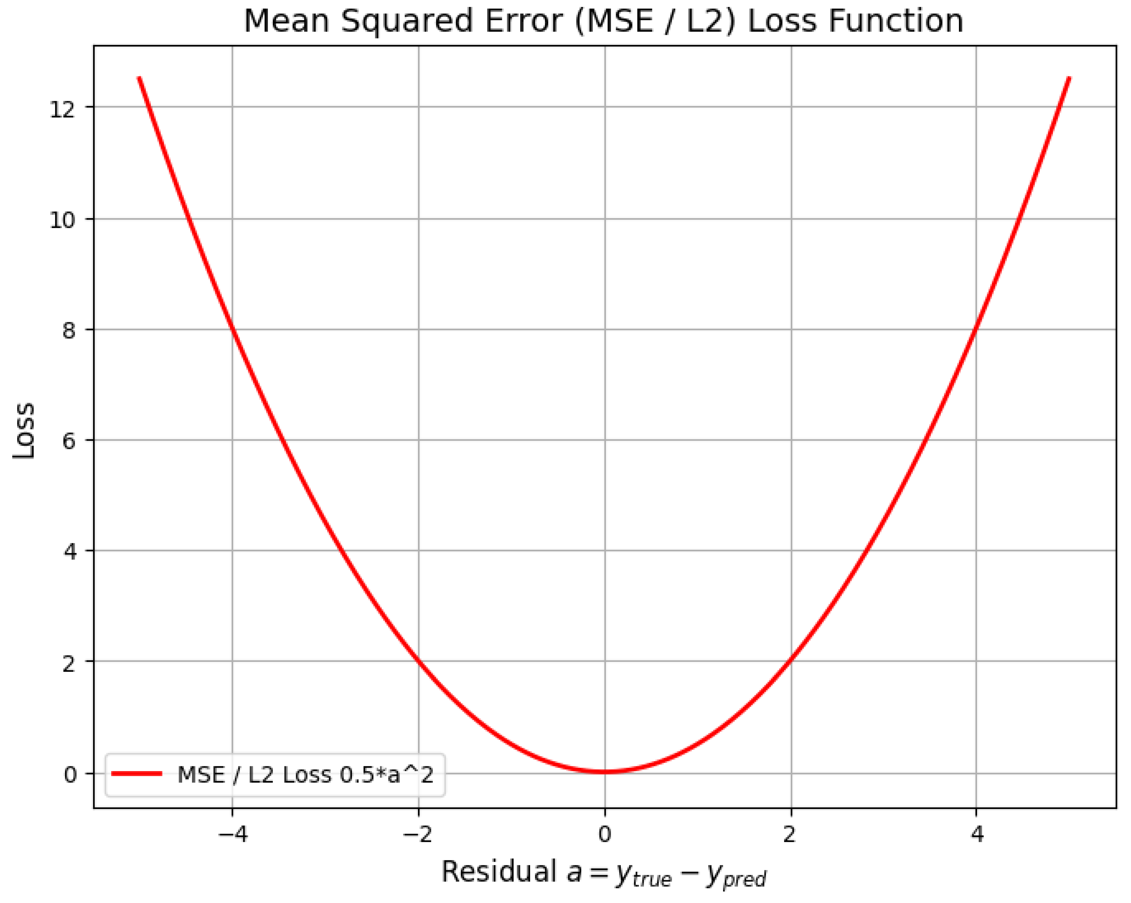
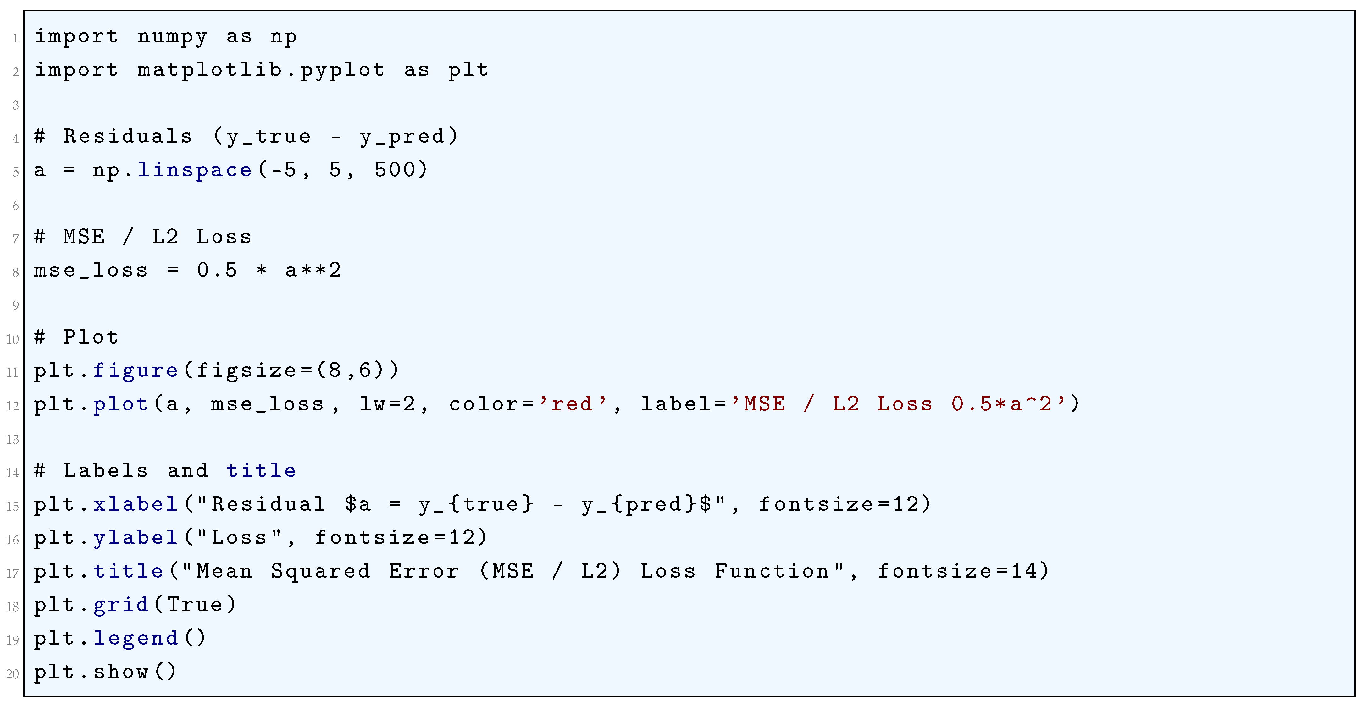
The Python code below produces the Figure 65 illustrating Mean Squared Error (MSE/L2) Loss Function.
10.5.1.5 Python Code to Generate Figure 66 Illustrating Mean Absolute Error (MAE/L1) Loss Function
The Python code below produces the Figure 66 illustrating Mean Absolute Error (MAE/L1) Loss Function.
Figure 66.
Mean Absolute Error (MAE/L1) Loss Function
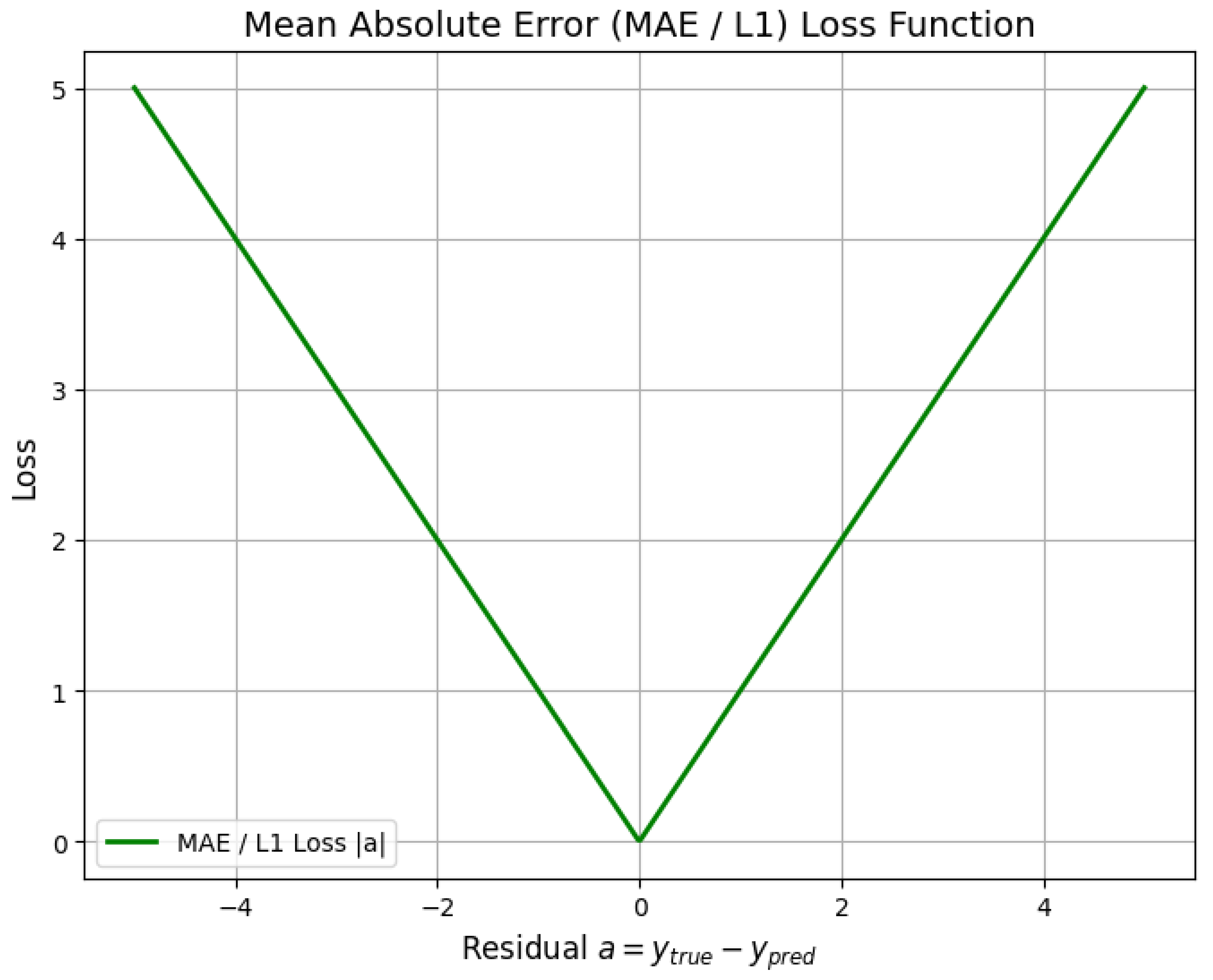
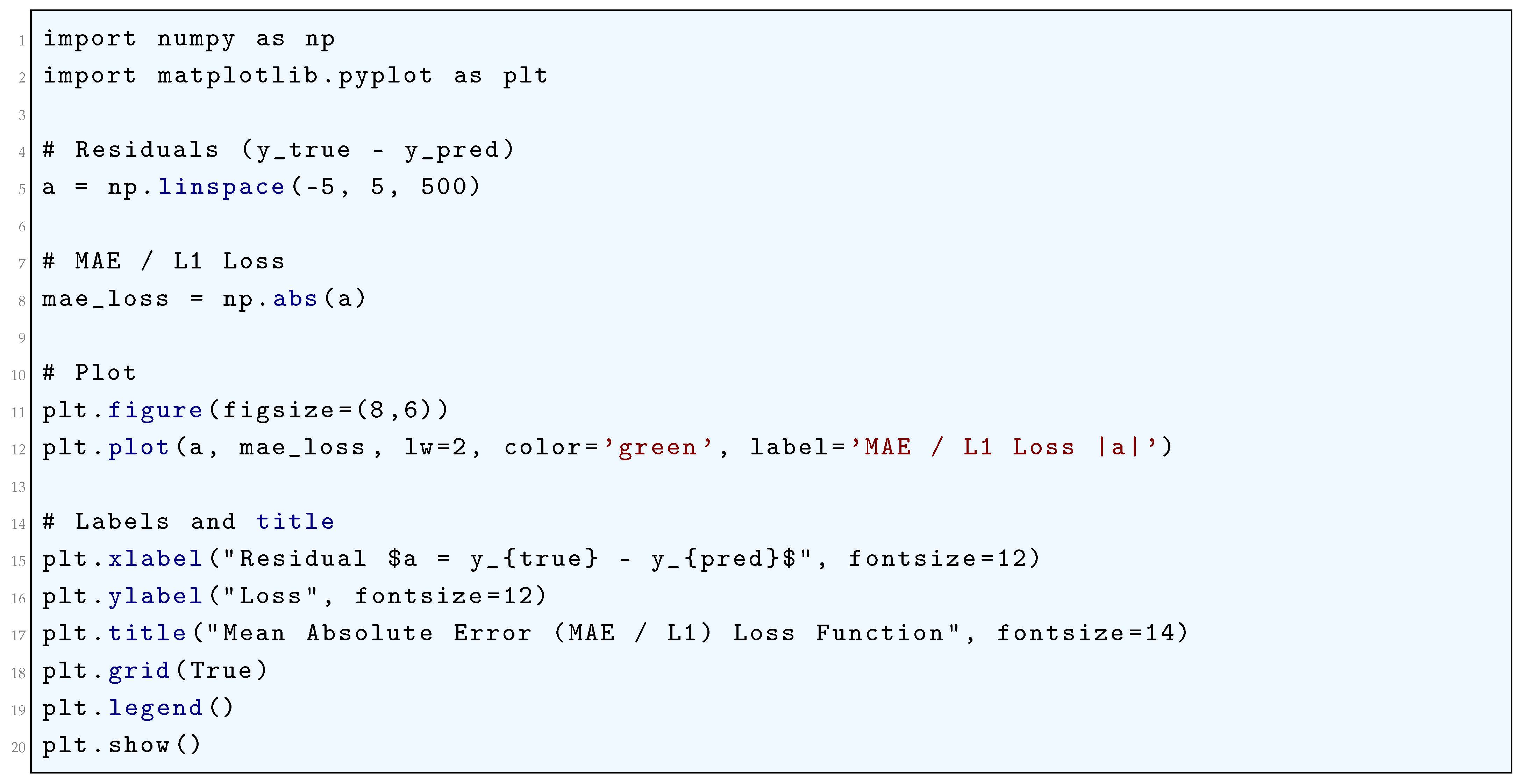
10.5.1.6 Python Code to Generate Figure 67 Illustrating Huber Loss Function
The Python code below produces the Figure 67 illustrating Huber Loss Function.
Figure 67.
Huber Loss Function
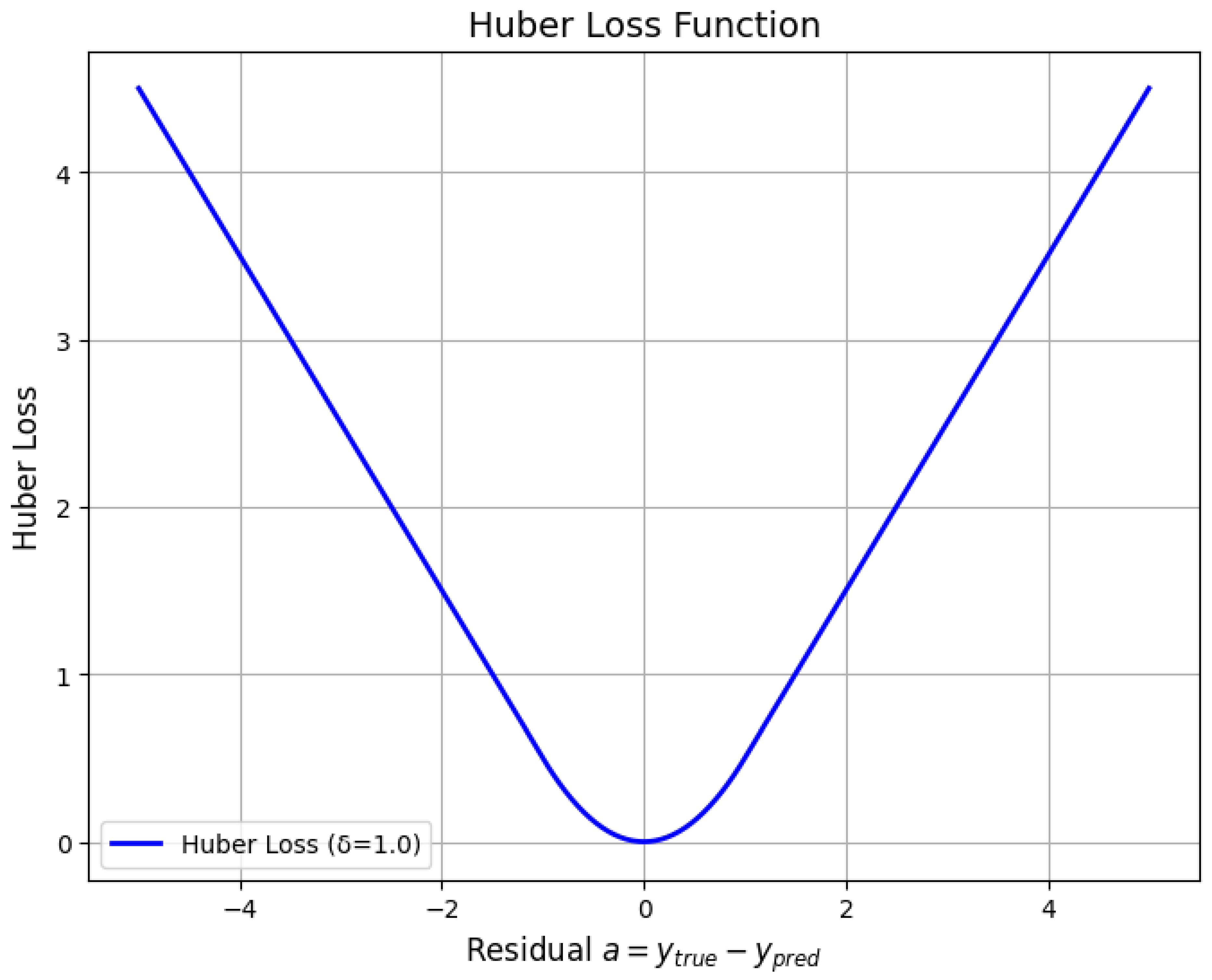
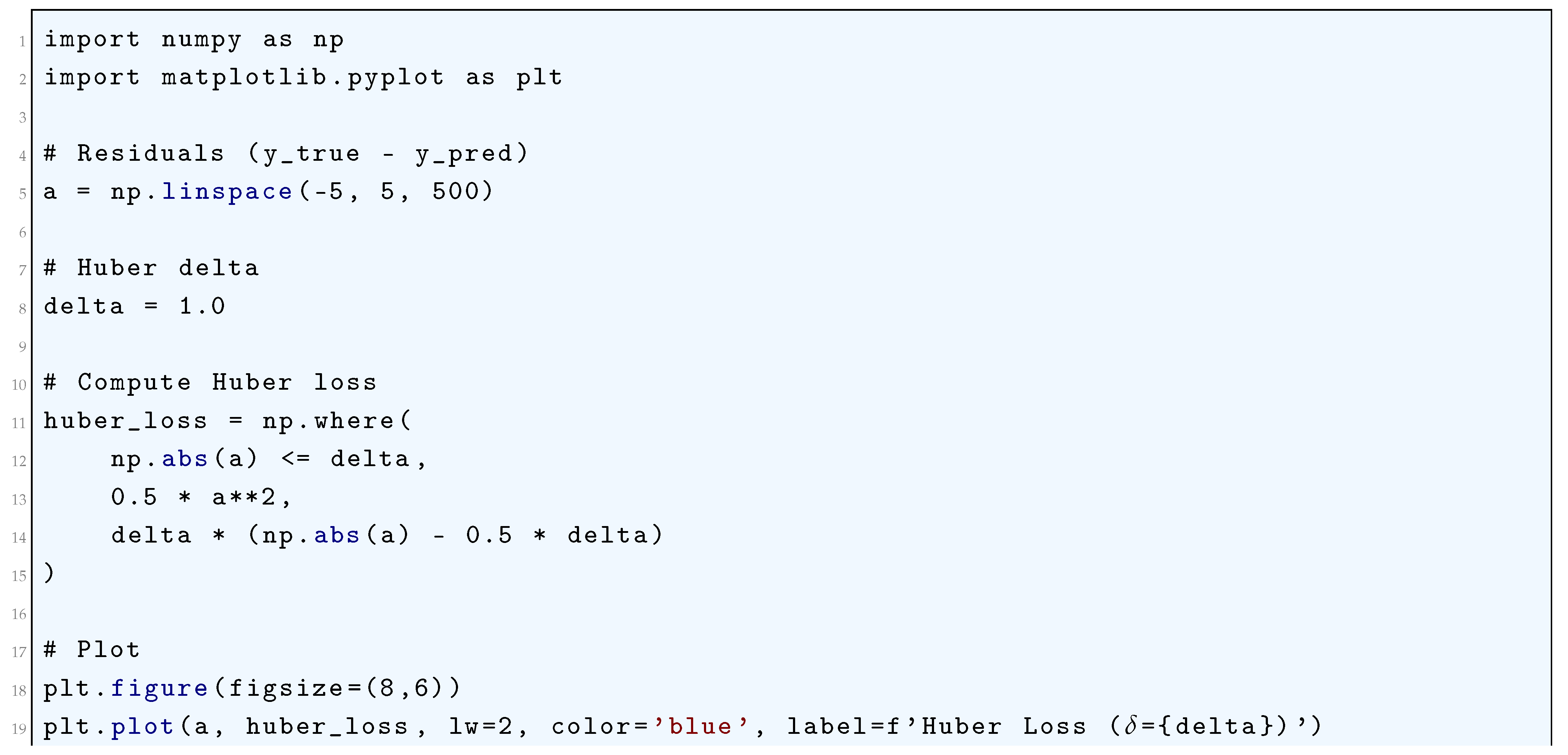
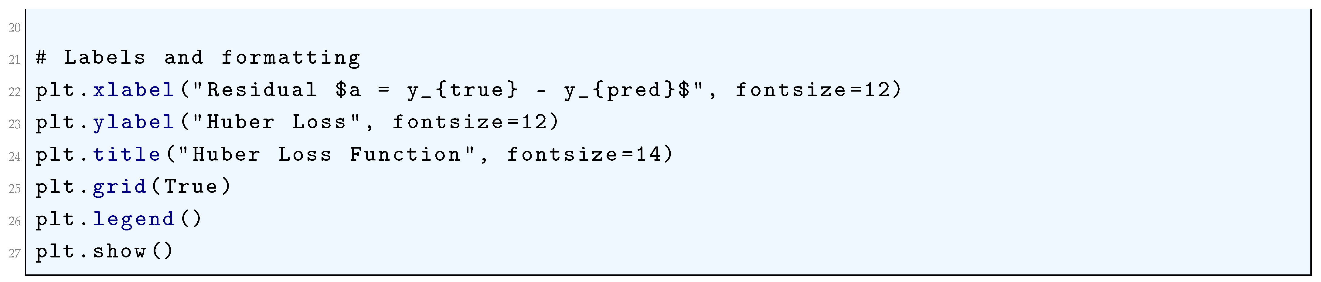
10.5.1.7 Python Code to Generate Figure 68 Comparing the Loss Functions: Huber, MSE, MAE
The Python code below produces the Figure 68 comparing the Loss Functions: Huber, MSE, MAE.
Figure 68.
Comparison of Loss Functions: Huber, MSE, MAE
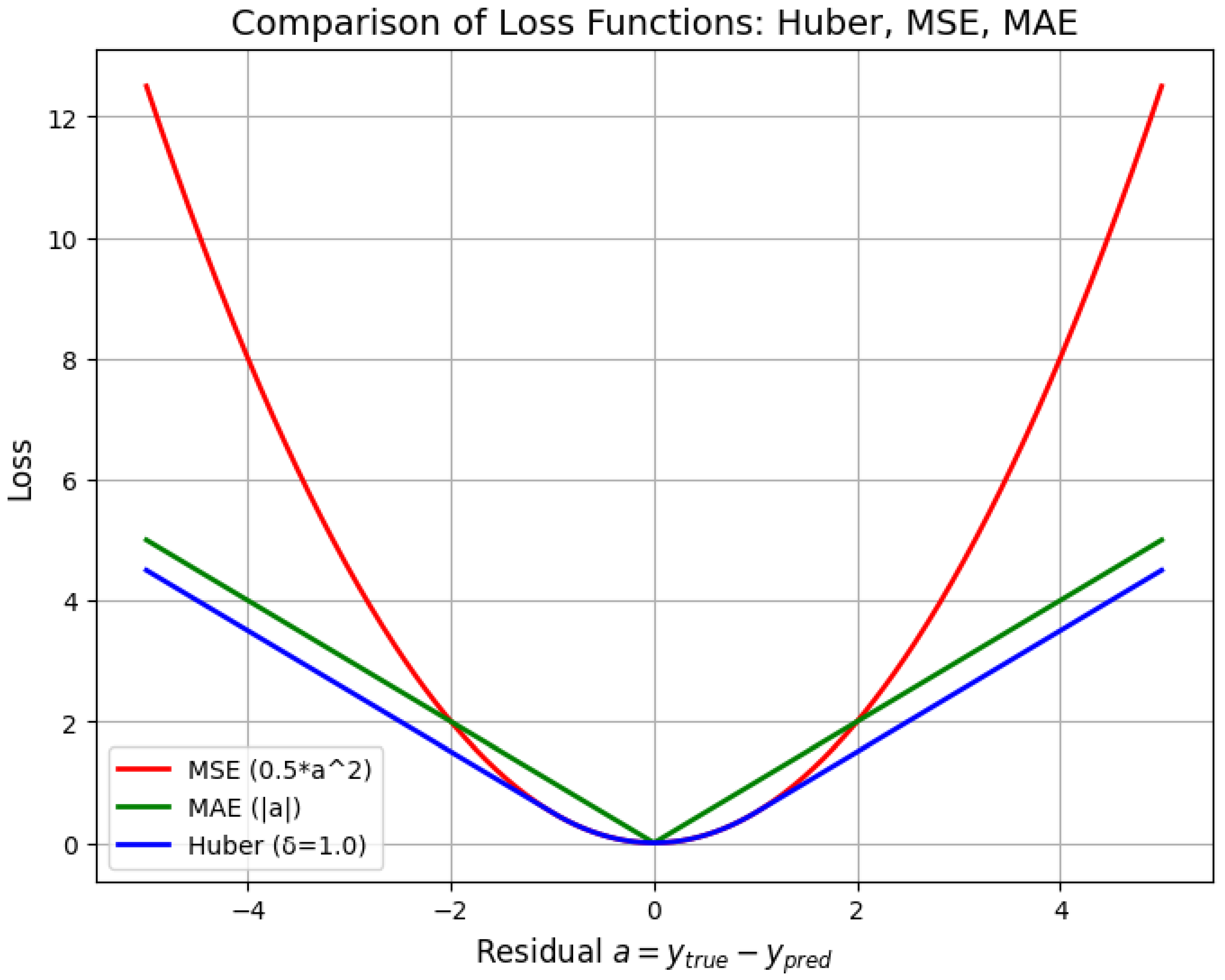
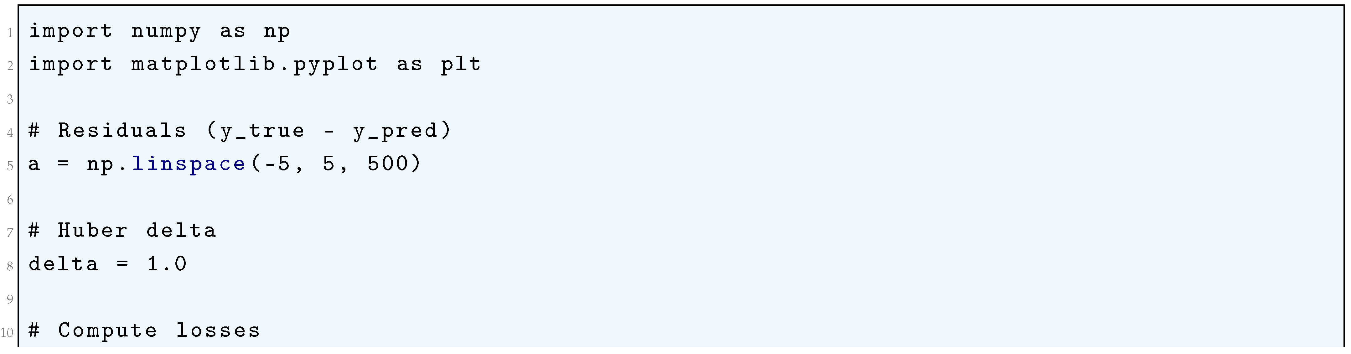
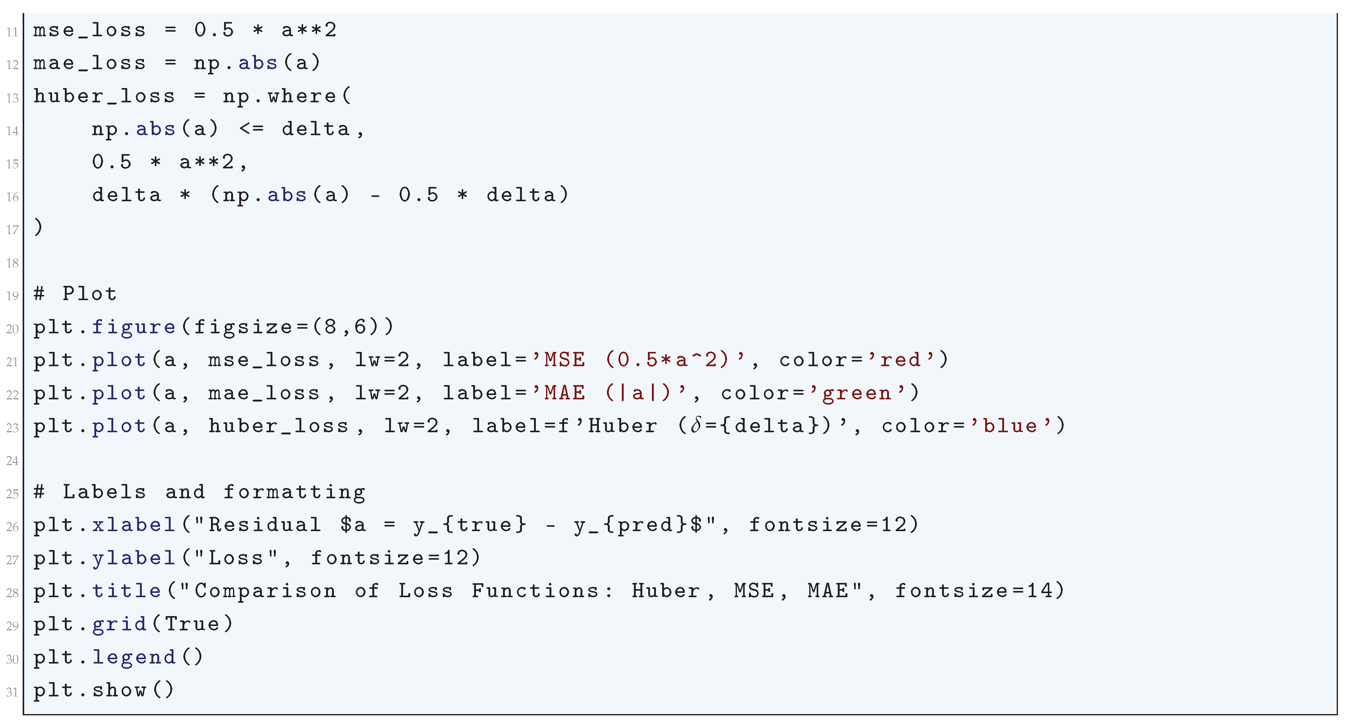
10.5.2. Loss Functions for Classification Tasks
For classification tasks, the cross-entropy loss is often employed, as it is particularly well-suited to tasks where the output is a probability distribution over multiple classes. In the binary classification case, where the target label is either 0 or 1, the binary cross-entropy loss function is defined as:
where is the predicted probability that the i-th sample belongs to the positive class (i.e., class 1). For multiclass classification, where the target label is a one-hot encoded vector representing the true class, the general form of the cross-entropy loss is:
where C is the number of classes, and is the predicted probability that the i-th sample belongs to class c. The gradient of the cross-entropy loss with respect to the predicted probabilities is:
This gradient facilitates the weight update by adjusting the model’s parameters to reduce the difference between the predicted probabilities and the actual class labels.
10.5.2.1 Binary Cross-Entropy (Log Loss)
The Binary Cross-Entropy loss function is the cornerstone of optimization for binary classification models, deriving its form directly from the principles of maximum likelihood estimation for a Bernoulli distribution. Consider a dataset of N independent and identically distributed observations, where the true labels are and the model’s prediction is the parameter , representing the estimated probability that . The probability of observing a single label given the input is given by the Bernoulli probability mass function:
The likelihood function for the entire dataset, assuming conditional independence, is the product of these probabilities:
The maximum likelihood estimate (MLE) for the parameters is found by maximizing this likelihood. To simplify this optimization, we take the natural logarithm, obtaining the log-likelihood:
Since optimization algorithms are typically designed for minimization, we define the loss function as the negative log-likelihood, scaled by to represent an empirical expectation over the data distribution:
Minimizing is thus equivalent to maximizing the likelihood of the observed data under the assumed Bernoulli model, ensuring the learned parameters yield a predicted probability distribution that is most consistent with the true labels.
From an information-theoretic perspective, Binary Cross-Entropy is the specific instance of the Kullback-Leibler (KL) Divergence between the empirical data distribution P and the model’s predictive distribution Q. For a single data point, the true distribution P is a degenerate Bernoulli distribution with parameter , having a probability mass of 1 at the true class. The model’s distribution Q is a Bernoulli distribution with parameter . The KL Divergence, which measures the information loss when Q is used to approximate P, is:
This expression can be decomposed as
The first term is the negative entropy of the true distribution . Since P is deterministic, , as is defined to be 0 by continuity and . Thus, the divergence simplifies to
The Binary Cross-Entropy loss is then the expectation of this divergence over the dataset:
The analytical properties of Binary Cross-Entropy are paramount for its use with gradient-based optimization.
The output of the neural network is typically produced by a sigmoid activation function applied to the final logit z, ensuring the prediction lies in the valid probability range :
The gradient of the loss with respect to the logit z exhibits a crucial simplification. We compute this gradient using the chain rule. First, the partial derivative of the loss for a single term with respect to the prediction is:
The derivative of the sigmoid activation with respect to its input is well-known:
Applying the chain rule, the gradient of the loss with respect to the logit is:
Distributing the terms yields:
This results in the elegant and stable gradient formula:
This simplicity is a key advantage. The gradient is merely the error between the prediction and the true label. Its magnitude is proportional to the error, providing a strong, clear signal for weight updates through backpropagation. The Hessian matrix, which contains the second derivatives, can be derived from this gradient. For a single data point, the second derivative with respect to the logit is
for , confirming the loss is convex with respect to the input logit . This local convexity contributes to the stable convergence properties of the optimization process when using this loss function.
10.5.2.2 Categorical Cross-Entropy
Categorical Cross-Entropy is the generalization of binary cross-entropy to multi-class classification problems where each instance belongs to exactly one of mutually exclusive classes. Its derivation is rooted in maximum likelihood estimation for the multinomial distribution. For a single data point, the true label is represented by a one-hot encoded vector , where if the instance belongs to class k and 0 otherwise. The model’s output is a probability distribution over the K classes, typically obtained using a softmax activation function on the final layer’s logits . The softmax function is defined as
which ensures and . The probability of observing the true label under this categorical model is given by the multinomial PMF for a single trial:
The likelihood for the entire dataset of N independent observations is
The log-likelihood is
The Categorical Cross-Entropy loss is consequently defined as the negative log-likelihood, scaled by the sample size:
Minimizing this loss is equivalent to maximizing the likelihood of the data, forcing the model’s predicted distribution to converge towards the true data distribution, which is a point mass at the correct class.
The information-theoretic interpretation of Categorical Cross-Entropy is that it computes the expected Kullback-Leibler Divergence between the true distribution P and the model’s distribution Q for each data point. For a single instance, the true distribution P is a categorical distribution with all probability mass on the true class , so where is the Kronecker delta. The model’s distribution Q is defined by . The KL Divergence is:
The terms are defined as 0 by continuity. This is identical to the inner sum for a one-hot vector , as only the term for is non-zero. Therefore, the loss
is the average KL Divergence across the dataset, measuring the total information loss when using the model’s distribution Q to approximate the true data distribution P.
The gradient of the Categorical Cross-Entropy loss with respect to the logits is particularly elegant and central to its use in backpropagation. The loss for a single sample is
To compute , we must account for the softmax function, as each logit influences every output due to the normalization in the denominator. The partial derivative of the softmax output for class k with respect to the logit for class j is:
where is the Kronecker delta. Using the chain rule, the gradient of the loss with respect to a specific logit is:
This sum can be separated:
Since is a one-hot vector, . This leads to the profoundly simple and stable result:
This gradient
is a vector whose j-th component is simply the difference between the predicted probability and the true label for class j. This elegant form ensures that the error signal propagated backwards during training is directly proportional to the discrepancy between the entire predicted distribution and the true distribution, providing a strong and clear direction for parameter updates. The Hessian of the loss with respect to the logits can be derived from this gradient and is related to the covariance of the predicted distribution, but the simplicity of the first-order gradient is its most critical property for efficient optimization in deep learning.
10.5.2.3 Sparse Categorical Cross-Entropy
Sparse Categorical Cross-Entropy is a computationally optimized variant of the standard Categorical Cross-Entropy loss function, designed for multi-class classification tasks where the true labels are provided as integer indices rather than one-hot encoded vectors. This formulation is mathematically equivalent to Categorical Cross-Entropy in its underlying probabilistic foundation but differs in its implementation, leading to significant gains in memory efficiency and computational speed, particularly when the number of classes K is very large. The fundamental principle remains maximum likelihood estimation for a categorical distribution. For a dataset of N samples, the true label for the i-th sample is given as an integer , which implicitly defines a degenerate probability distribution where and is the Kronecker delta. The model, as in the non-sparse case, produces a probability distribution over the K classes via the softmax function applied to a vector of logits :
The likelihood of observing the true label is , and the corresponding negative log-likelihood for a single sample is
The full Sparse Categorical Cross-Entropy loss is then the empirical expectation of this negative log-likelihood:
This is computationally and notationally more efficient than the standard form
because it avoids the explicit construction and storage of the entire matrix of one-hot encodings, requiring only the storage of an integer vector of length N for the labels. The minimization of this loss function is identical to minimizing the KL Divergence
for each sample, where is the model’s distribution.
The gradient computation for Sparse Categorical Cross-Entropy, crucial for backpropagation, reveals its intimate connection to the standard formulation while highlighting its efficiency. The gradient of the loss for a single sample with respect to the logits must be computed. This requires the partial derivative for any class j. The derivative of the loss with respect to the predicted probability of the true class is
The connection to all logits is made through the Jacobian of the softmax function
Applying the chain rule, the gradient for an arbitrary logit is:
This results in the same elegantly simple gradient vector as the standard formulation:
where is now the implicit one-hot vector corresponding to the integer label , meaning its j-th component is .
From an implementation perspective, this means the gradient for the logit corresponding to the true class is , and for all other logits , it is simply . This result is identical to the gradient derived for the one-hot encoded case; however, the computational pathway to achieve it is more efficient. There is no need to materialize a full one-hot matrix, perform a large matrix multiplication, or sum over all K classes for each sample during the gradient calculation. The backward pass can be implemented by first computing the softmax probabilities , then copying this entire vector as the gradient , and finally subtracting 1 from the single element at the index of the true label . This operation is per sample, but the constant factors and memory overhead are drastically lower than in the one-hot case, making Sparse Categorical Cross-Entropy the preferred choice in practice for problems with a large number of classes, such as in language modeling or large-scale image classification.
10.5.2.4 Kullback-Leibler Divergence (KL Divergence)
The Kullback-Leibler (KL) Divergence, denoted , is a fundamental measure of information theory that quantifies the difference between two probability distributions P and Q over the same random variable X. It is not a true metric, as it is not symmetric and does not satisfy the triangle inequality; rather, it is a divergence that measures the information loss when a distribution Q is used to approximate the true distribution P. For discrete distributions, the KL Divergence is defined as
where is the sample space, and the sum is taken over all possible values of X. For continuous distributions, the definition involves an integral:
where p and q are the probability density functions of P and Q, respectively. The logarithm is typically taken with base 2 (yielding units of bits) or base e (yielding units of nats), and by convention, and for , reflecting the infinite penalty for assigning zero probability to an event that is possible under P. The divergence is always non-negative, , with equality if and only if almost everywhere, a result known as Gibbs’ inequality, which follows from the strict concavity of the logarithm function and Jensen’s inequality.
For a fixed discrete probability distribution P:
The plot of KL Divergence as a function of shall be
The KL Divergence can be decomposed into two interpretable components: the cross-entropy between P and Q minus the entropy of P. Cross-entropy measures the average number of bits needed to encode events from P using a code optimized for Q, defined as
for discrete variables. The entropy of P
measures the inherent uncertainty or the average number of bits needed to encode events from P using an optimal code. Thus
This decomposition shows that the divergence represents the extra number of bits required to encode data from P when using a code based on Q, rather than the true distribution P. In the context of machine learning, where P is often the true data distribution and Q is the model’s distribution, minimizing the KL Divergence is equivalent to minimizing the cross-entropy, since is fixed with respect to the model parameters. This is why cross-entropy loss is ubiquitously used in classification tasks.
For a fixed discrete probability distribution P:
The 2D plot of KL Divergence as a function of and shall be
The mathematical properties of the KL Divergence are critical for its applications. It is convex in both P and Q, meaning that for any two pairs of distributions and , and for , we have
This convexity ensures that optimization problems involving KL Divergence have unique minima under certain constraints. The divergence also factors elegantly for independent distributions. If and , then
Additivity extends to more complex factorizations, such as in variational inference, where it is used to approximate posterior distributions. The gradient of the KL Divergence with respect to the parameters of Q is essential for gradient-based optimization. For a parameterized distribution , we have
as the entropy of P is independent of . This gradient is the same as that of the cross-entropy loss, facilitating its use in training probabilistic models like variational autoencoders, where it acts as a regularizer to push the approximate posterior toward a prior distribution , ensuring tractable inference and meaningful latent representations.
10.5.2.5 Python Code to Generate Figure 69 Illustrating Binary Cross-Entropy (BCE) Loss Function
The Python code below produces the Figure 69 illustrating Binary Cross-Entropy (BCE) Loss Function.
Figure 69.
Binary Cross-Entropy (BCE) Loss Function
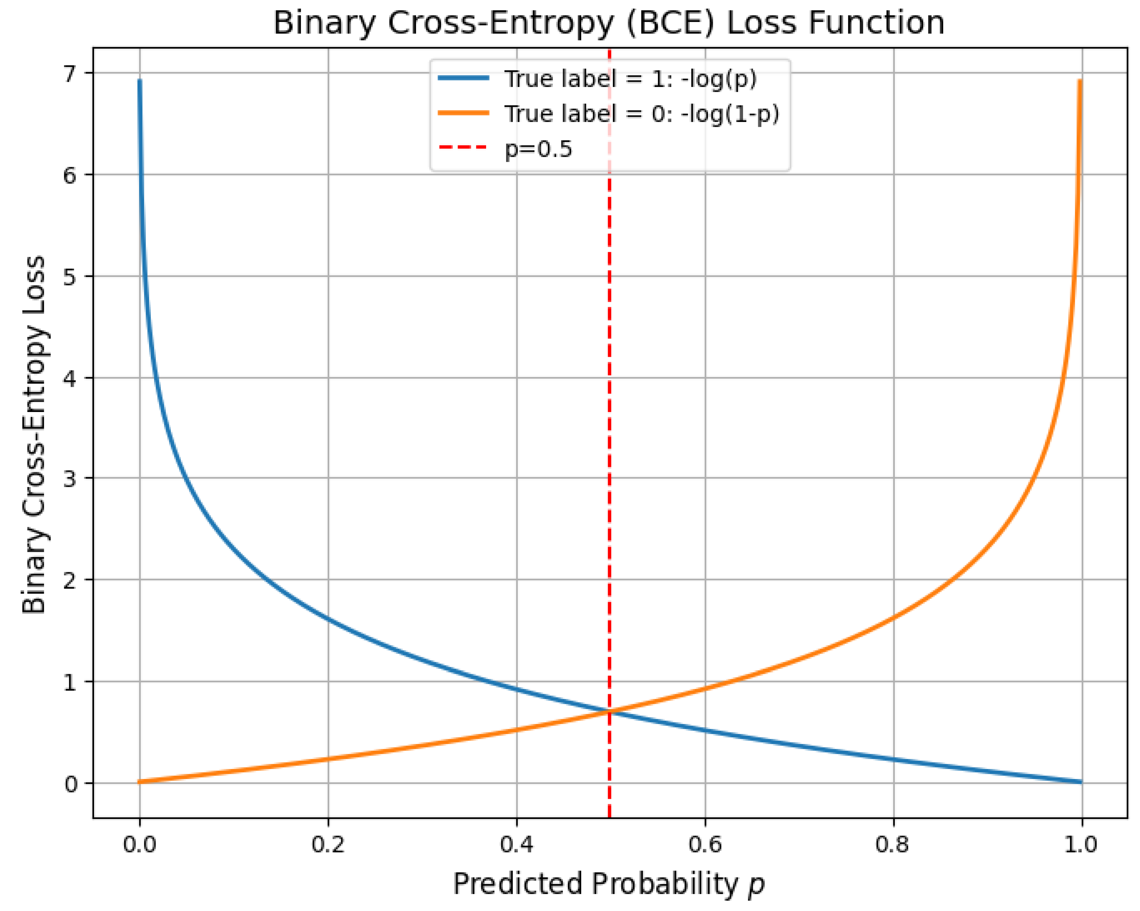
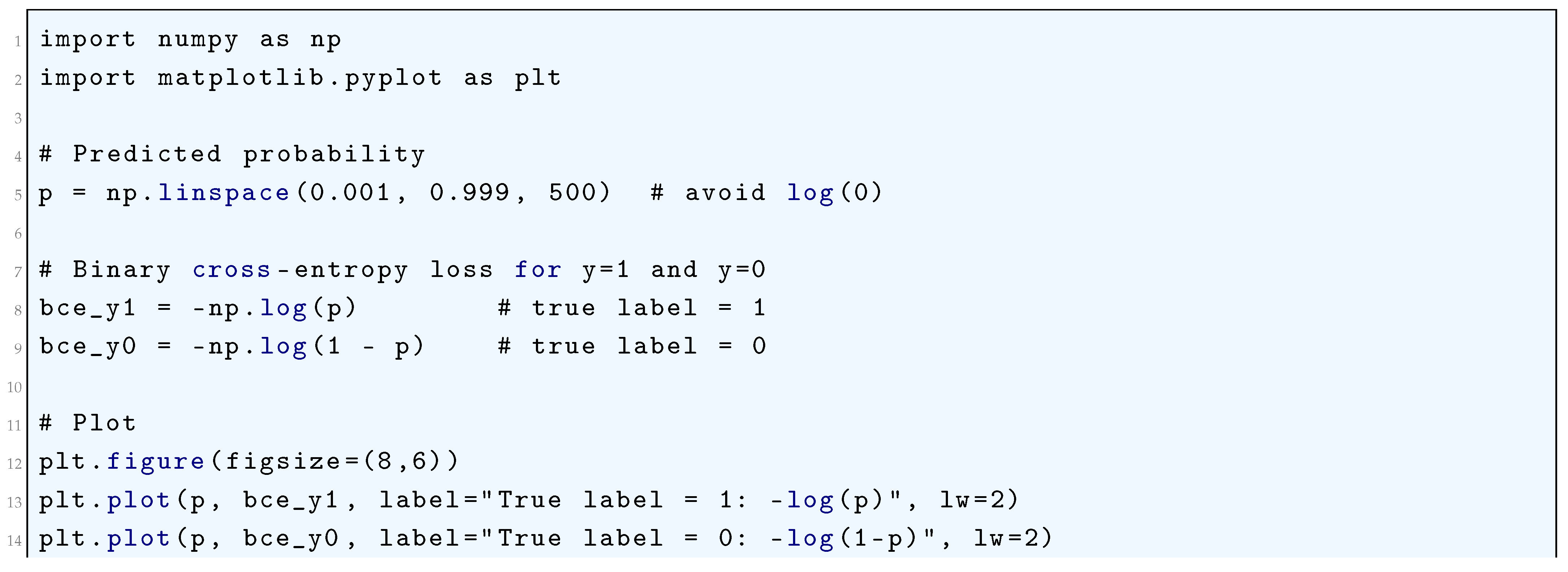
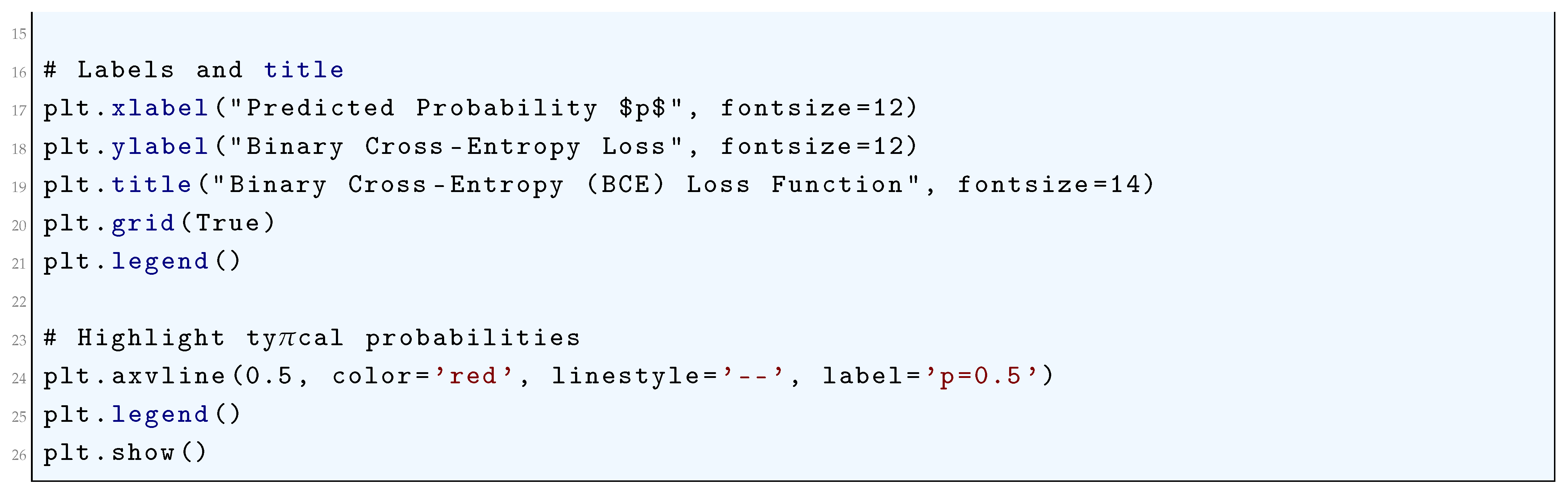
10.5.2.6 Python Code to Generate Figure 70 Illustrating Binary Cross-Entropy Loss Surface
The Python code below produces the Figure 70 illustrating Binary Cross-Entropy Loss Surface.
Figure 70.
Binary Cross-Entropy Loss Surface
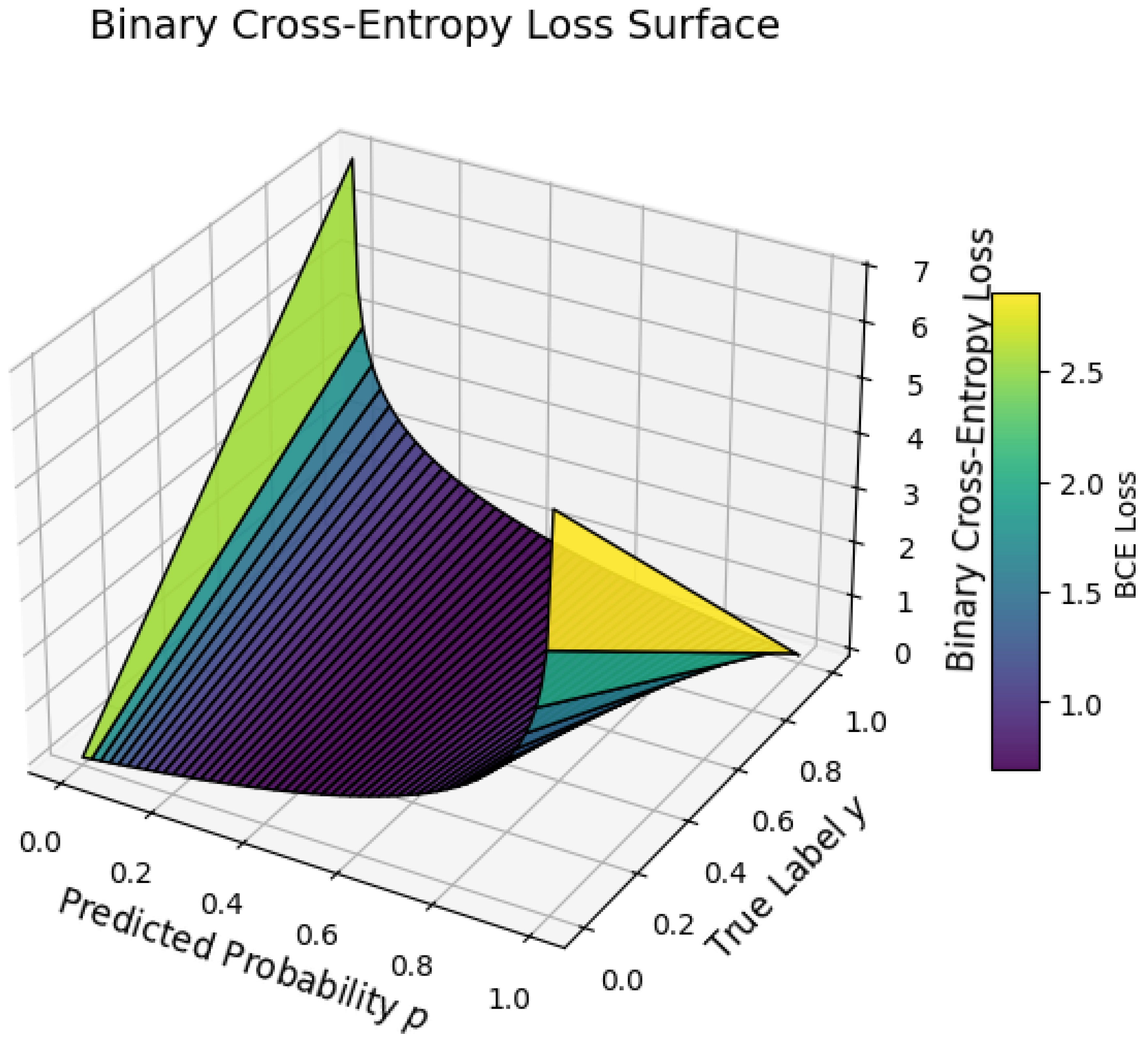
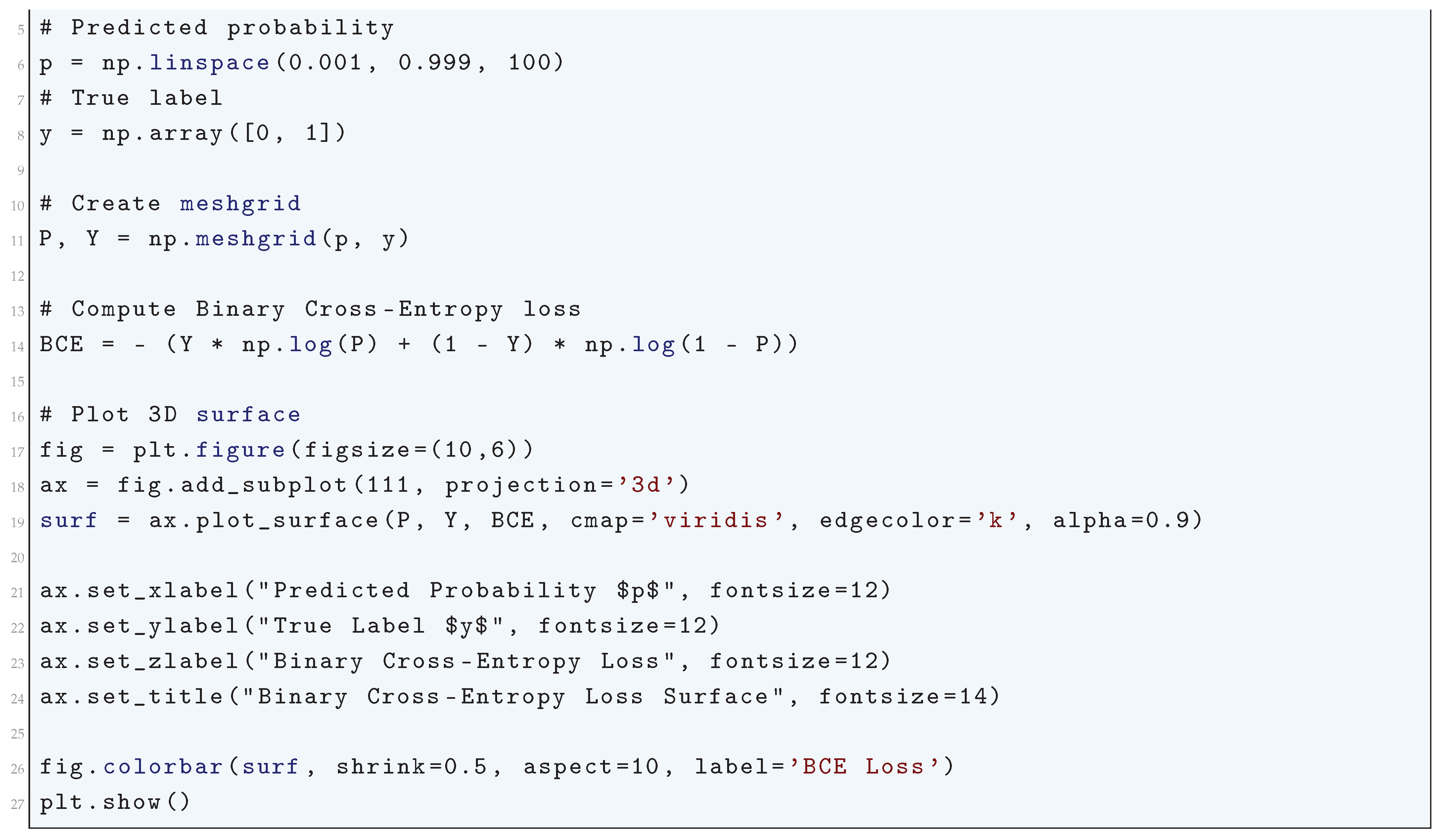
10.5.2.7 Python Code to Generate Figure 71 Illustrating Categorical Cross-Entropy Loss
The Python code below produces the Figure 71 illustrating Categorical Cross-Entropy Loss.
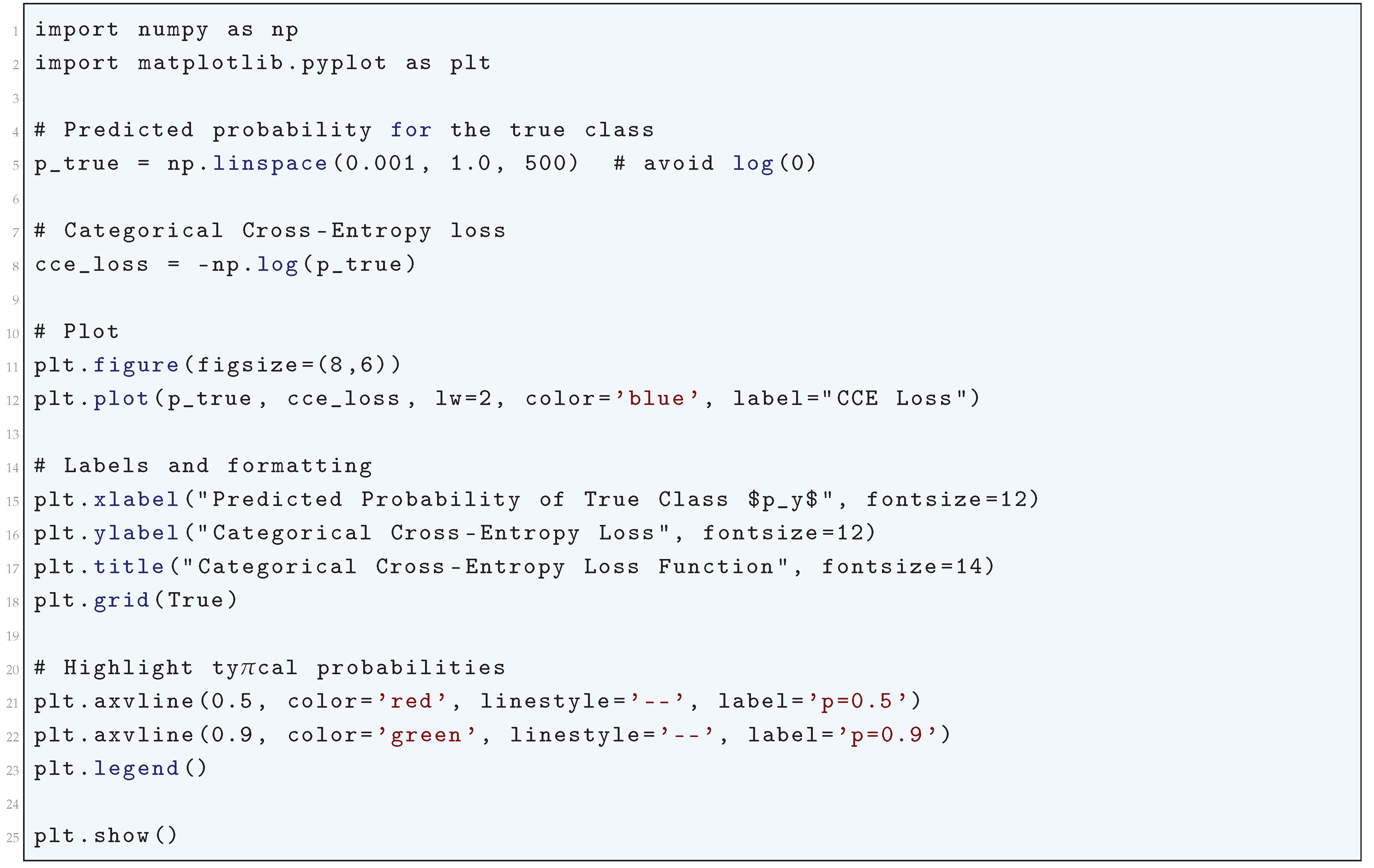
Figure 71.
Categorical Cross-Entropy Loss
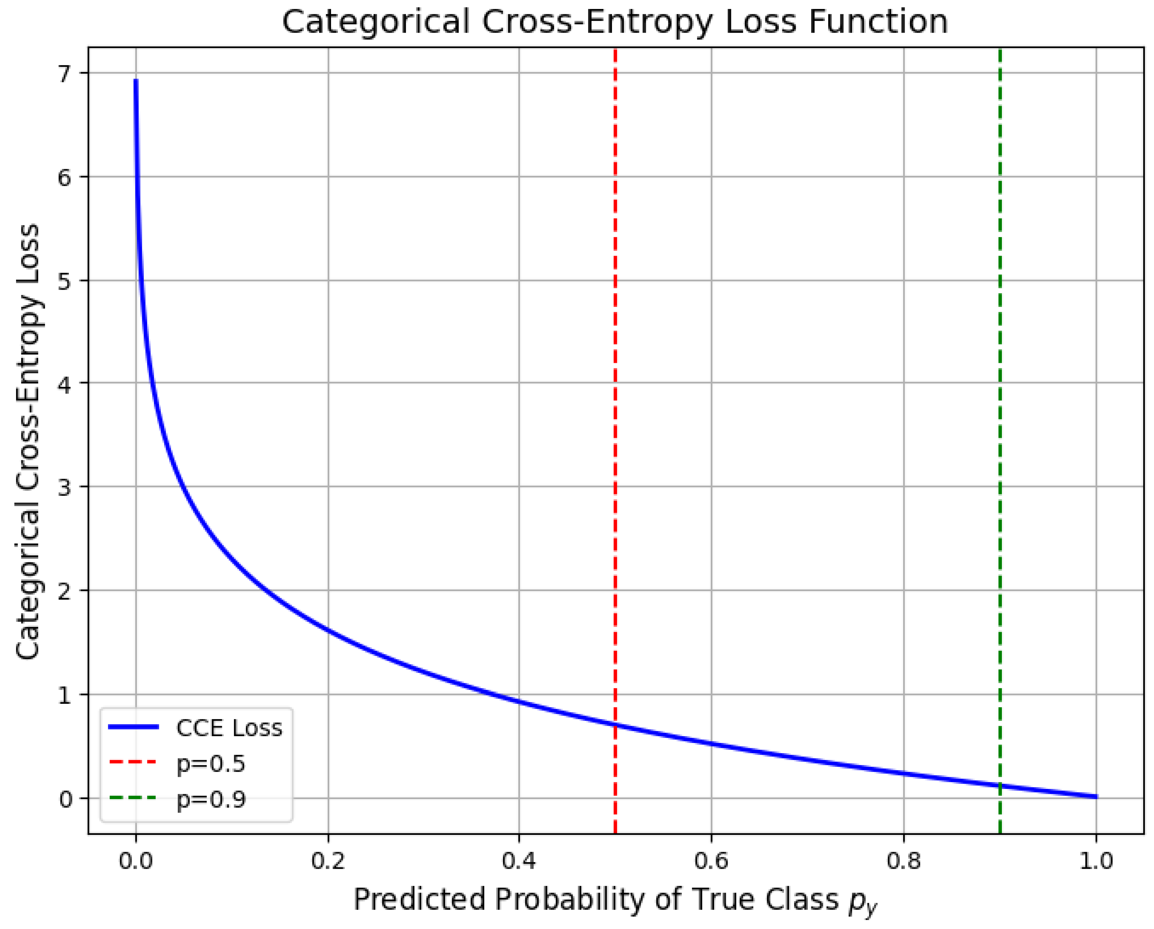
10.5.2.8 Python Code to Generate Figure 72 Illustrating Categorical Cross-Entropy Loss
The Python code below produces the Figure 72 illustrating Categorical Cross-Entropy Loss.
Figure 72.
Categorical Cross-Entropy Loss

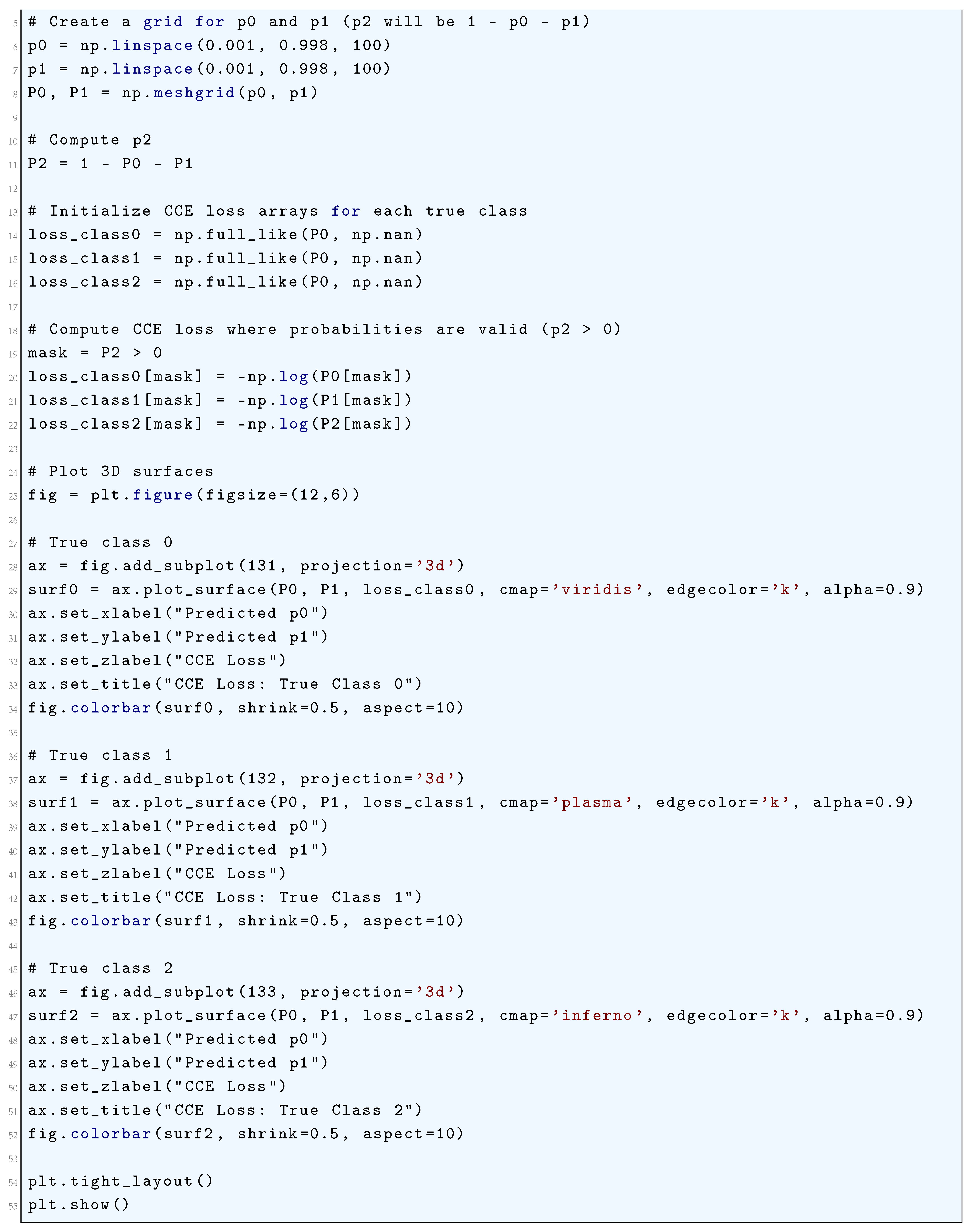
10.5.2.9 Python Code to Generate Figure 73 Illustrating Sparse Categorical Cross-Entropy Loss
The Python code below produces the Figure 73 illustrating Sparse Categorical Cross-Entropy Loss.
Figure 73.
Sparse Categorical Cross-Entropy Loss
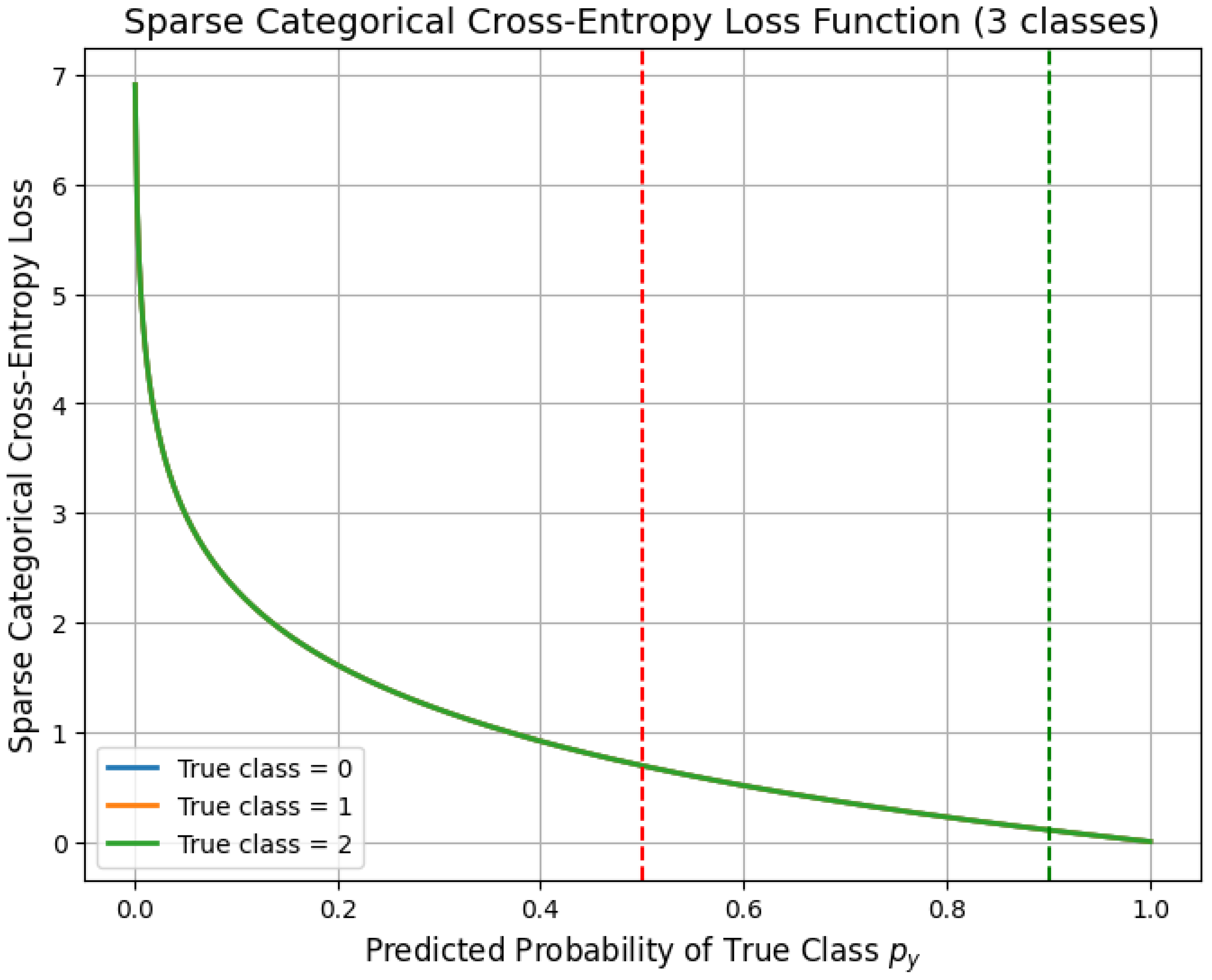
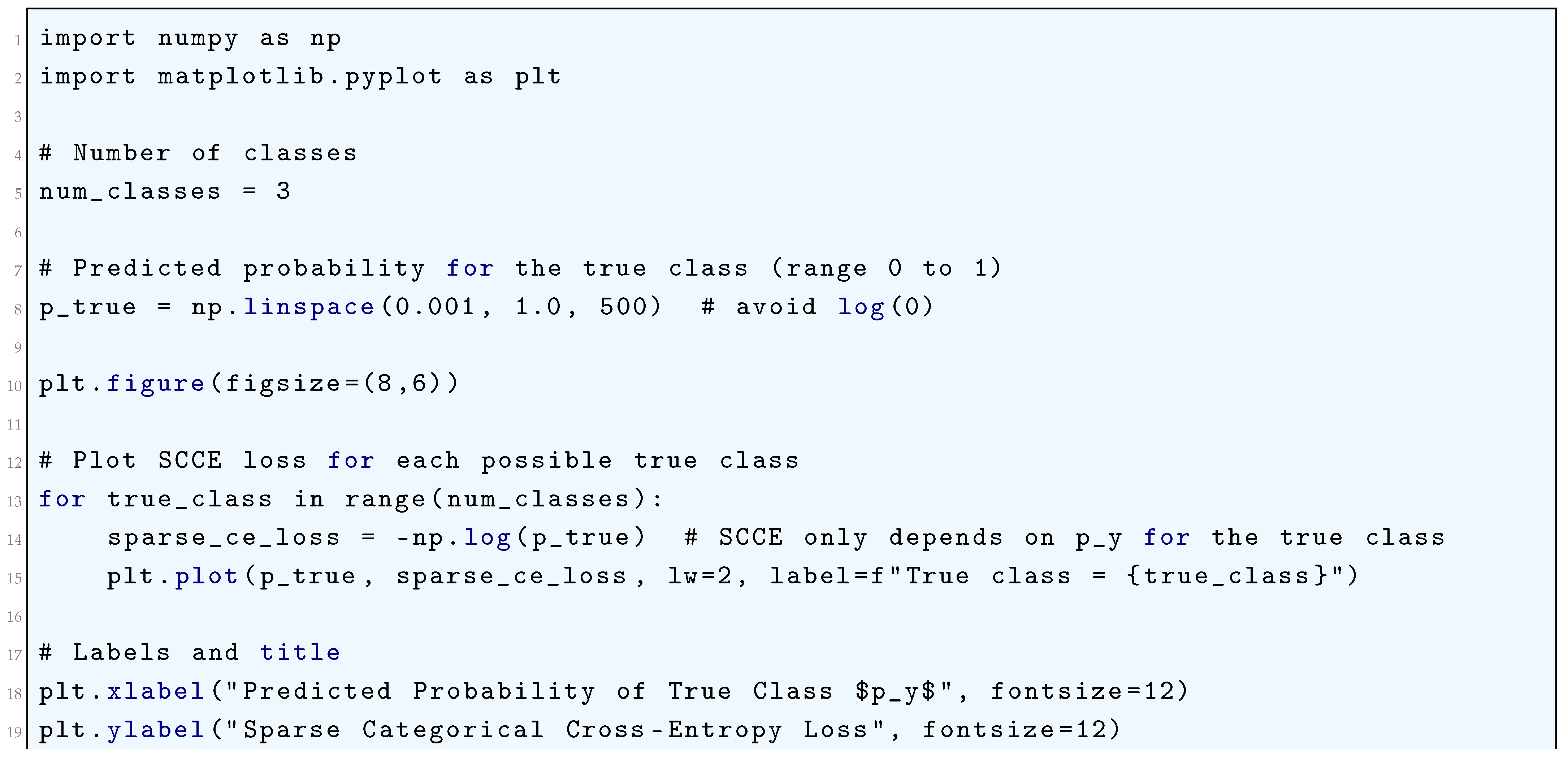
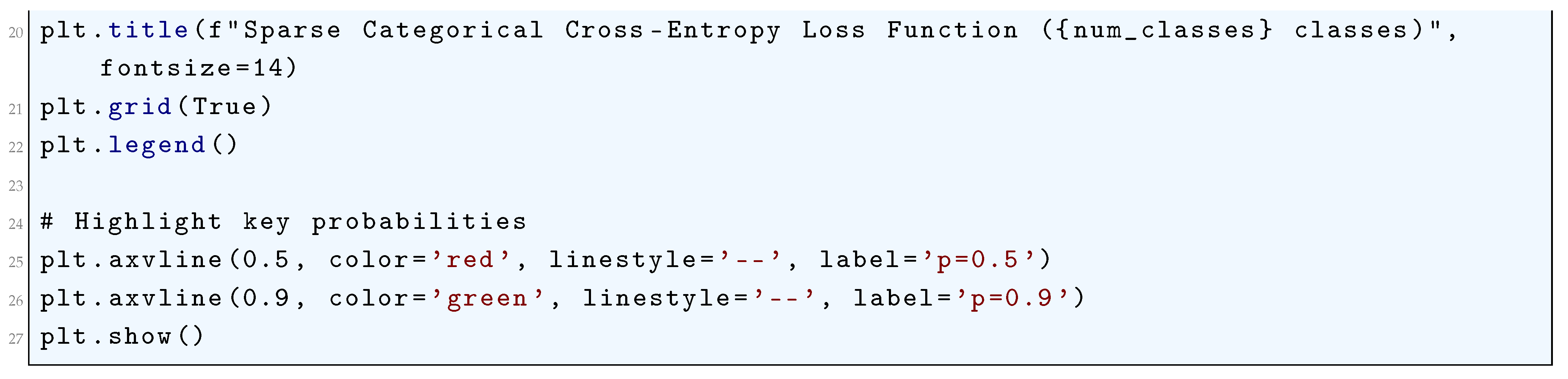
10.5.2.10 Python Code to Generate Figure 74 Illustrating Surface Plot of Sparse Categorical Cross-Entropy Loss
The Python code below produces the Figure 74 illustrating Surface Plot of Sparse Categorical Cross-Entropy Loss.
Figure 74.
Surface Plot of Sparse Categorical Cross-Entropy Loss
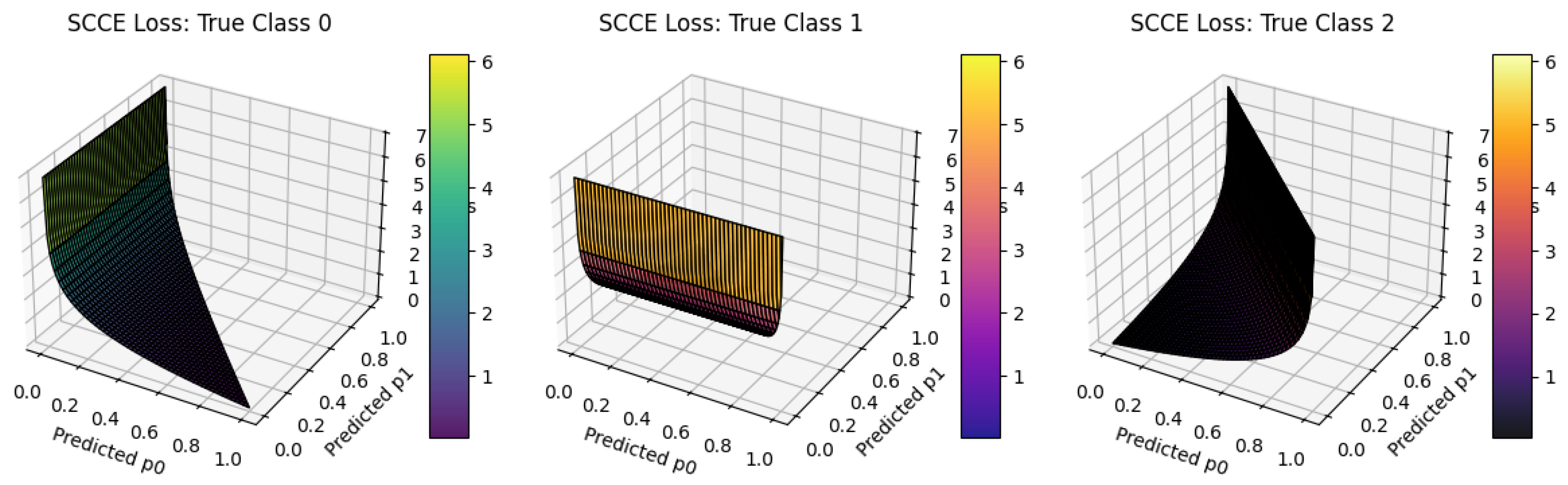
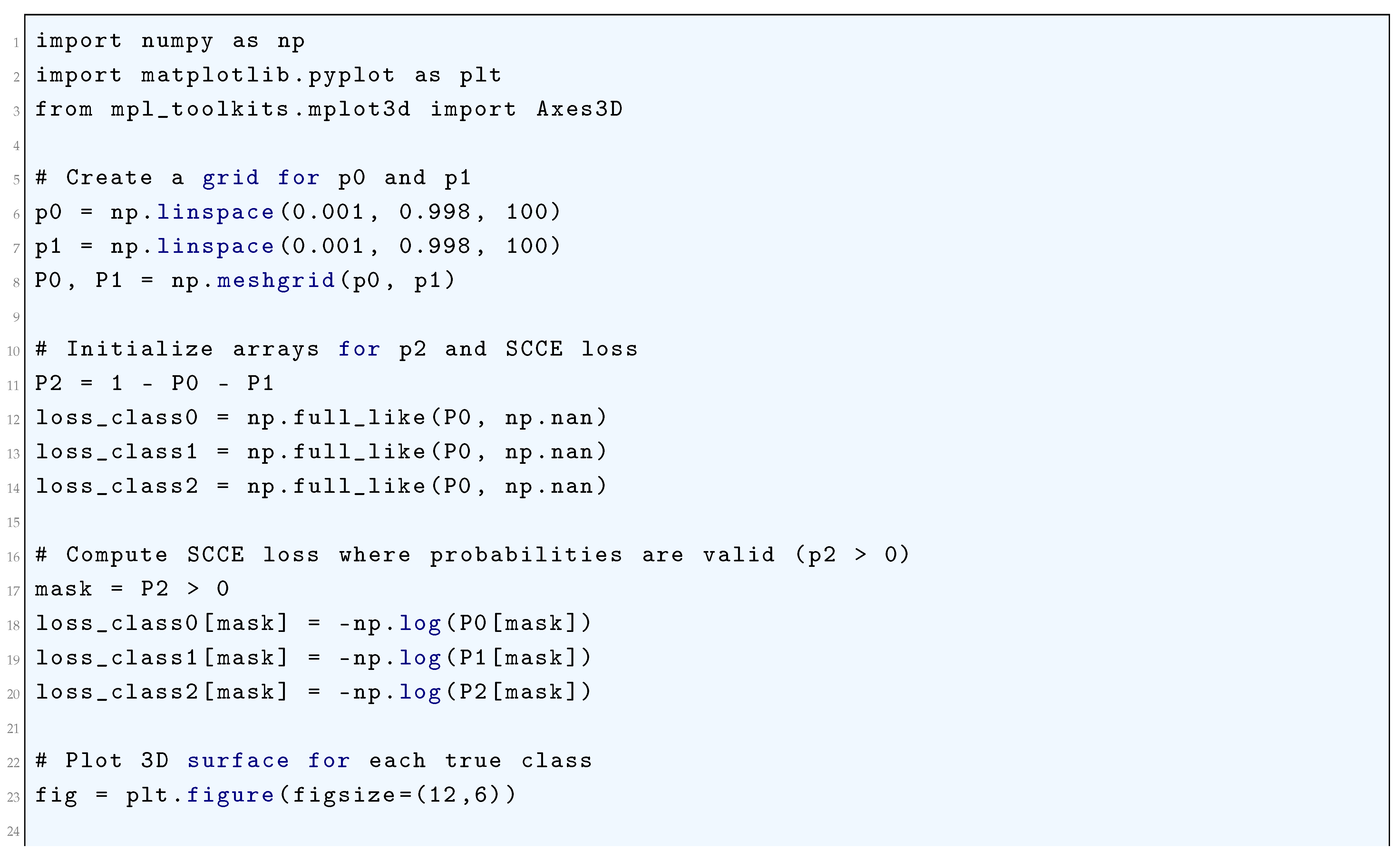
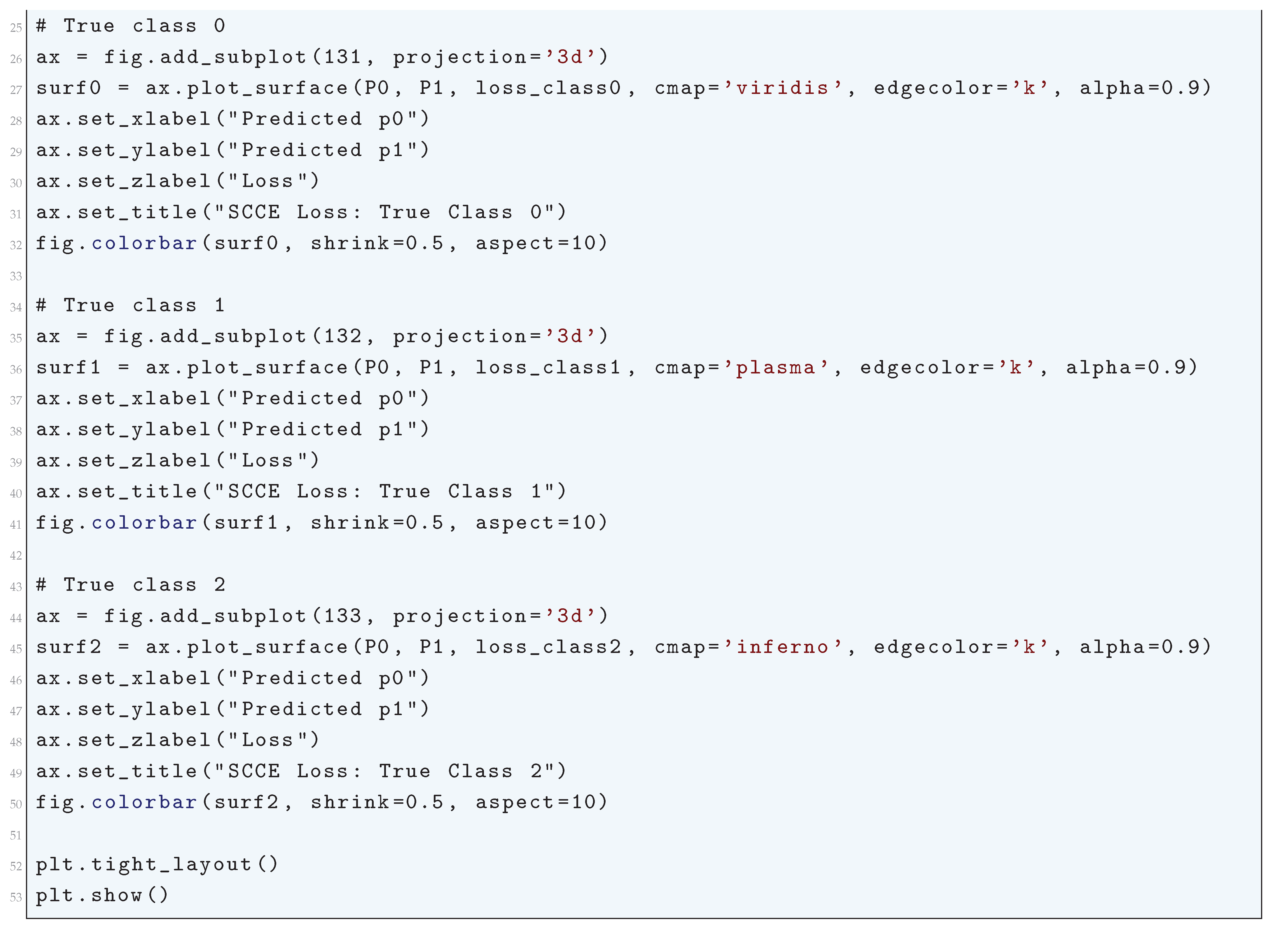
10.5.2.11 Python Code to Generate Figure 75 Illustrating KL Divergence
The Python code below produces the Figure 75 illustrating KL Divergence.
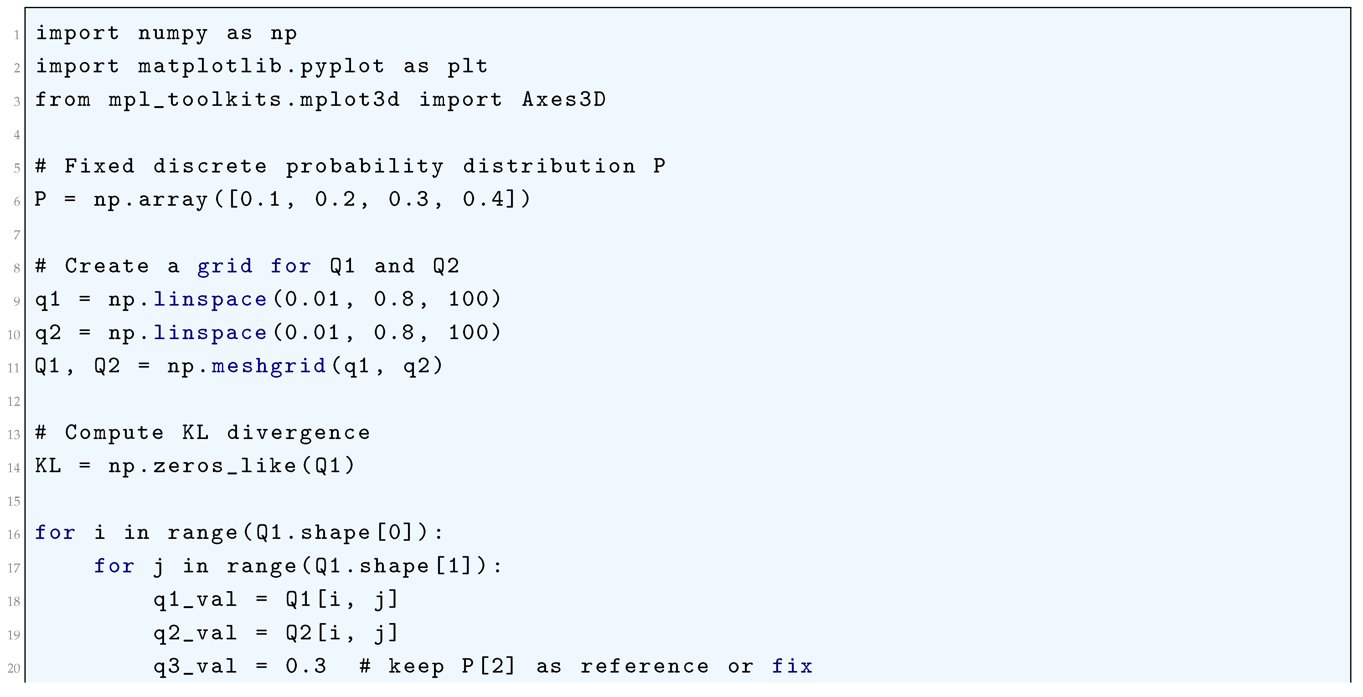
Figure 75.
Plot of KL Divergence
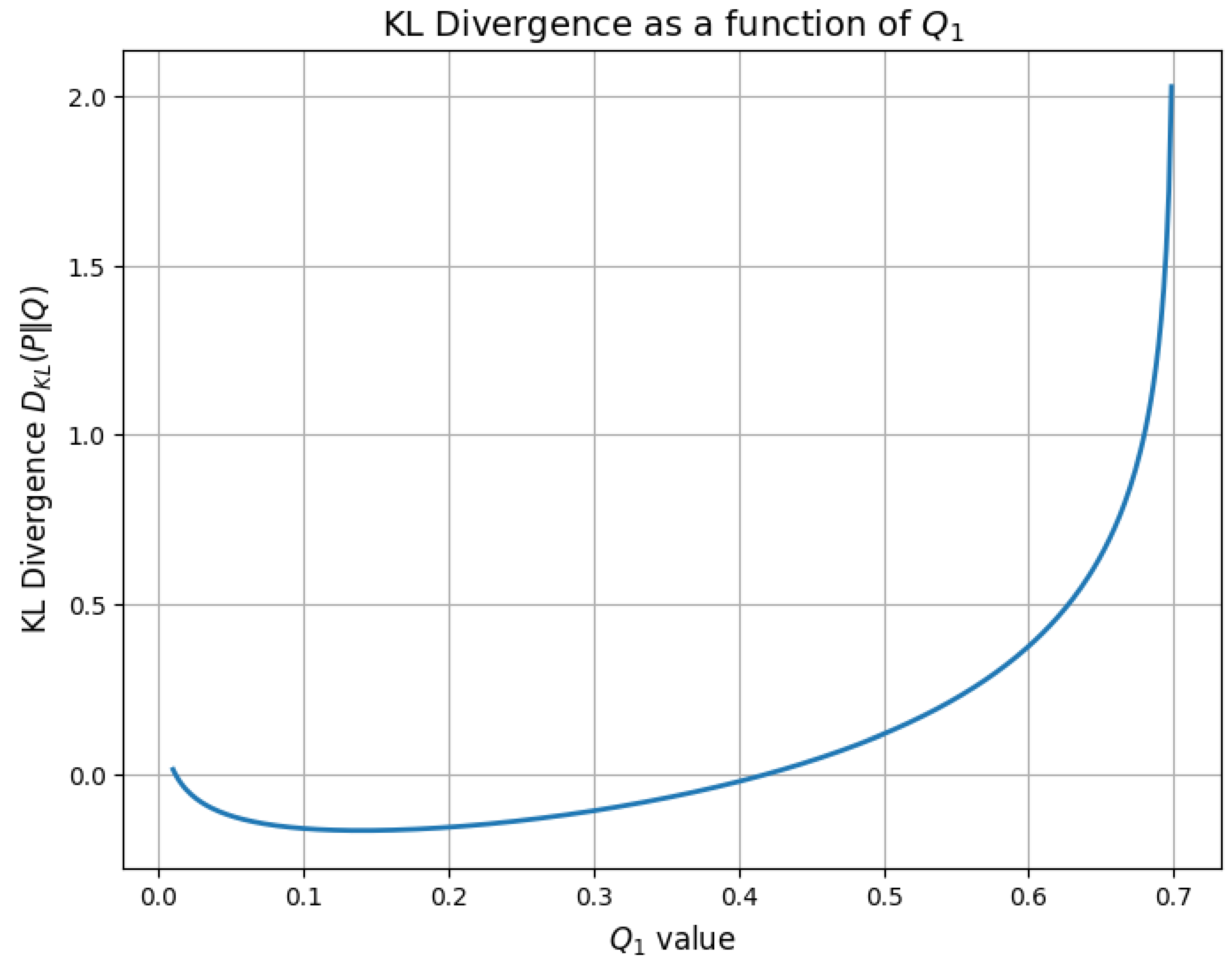
10.5.2.12 Python Code to Generate Figure 76 Illustrating 2D Surface Plot of KL Divergence
The Python code below produces the Figure 76 illustrating 2D Surface Plot of KL Divergence.
Figure 76.
2D Surface Plot of KL Divergence
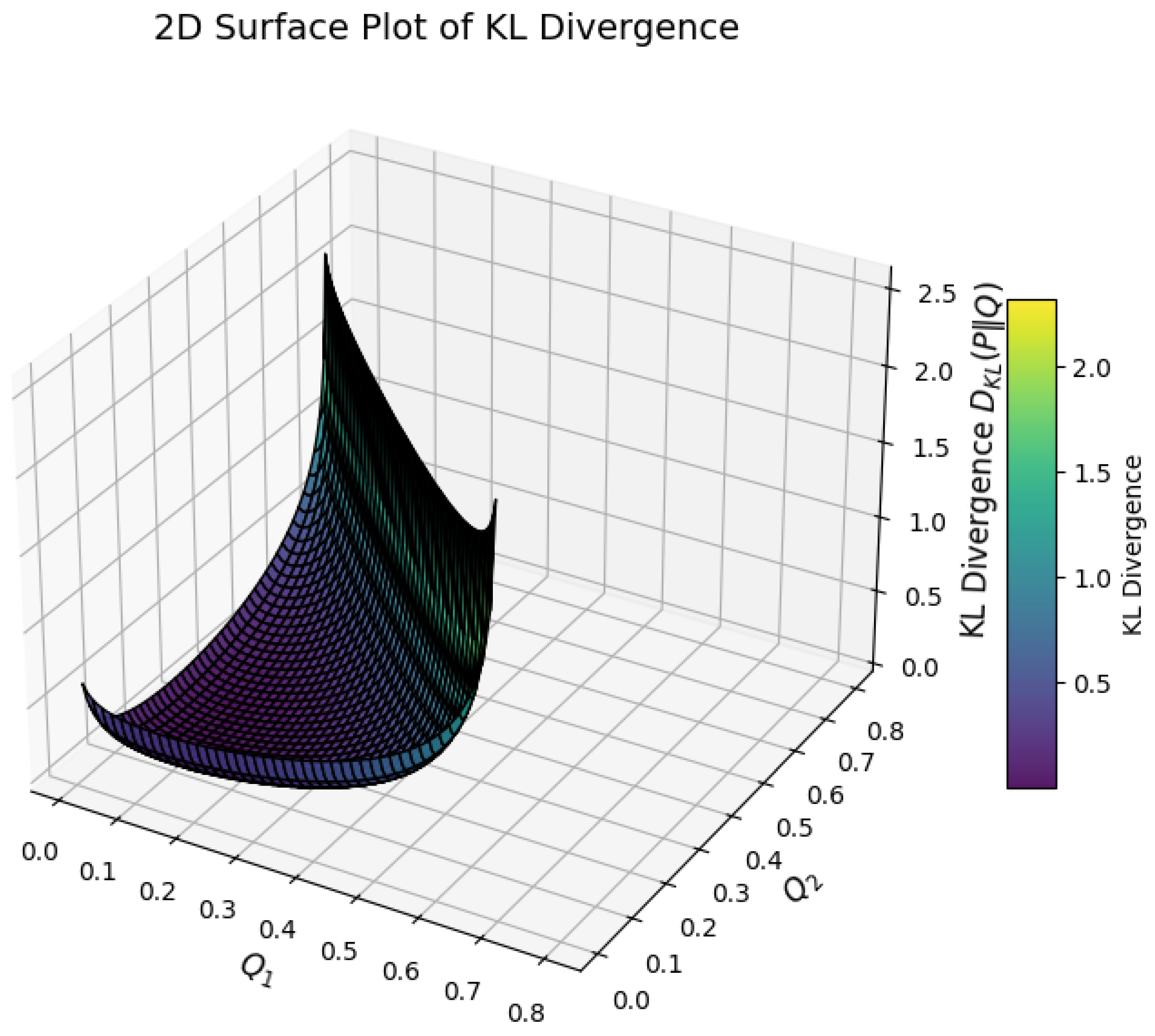
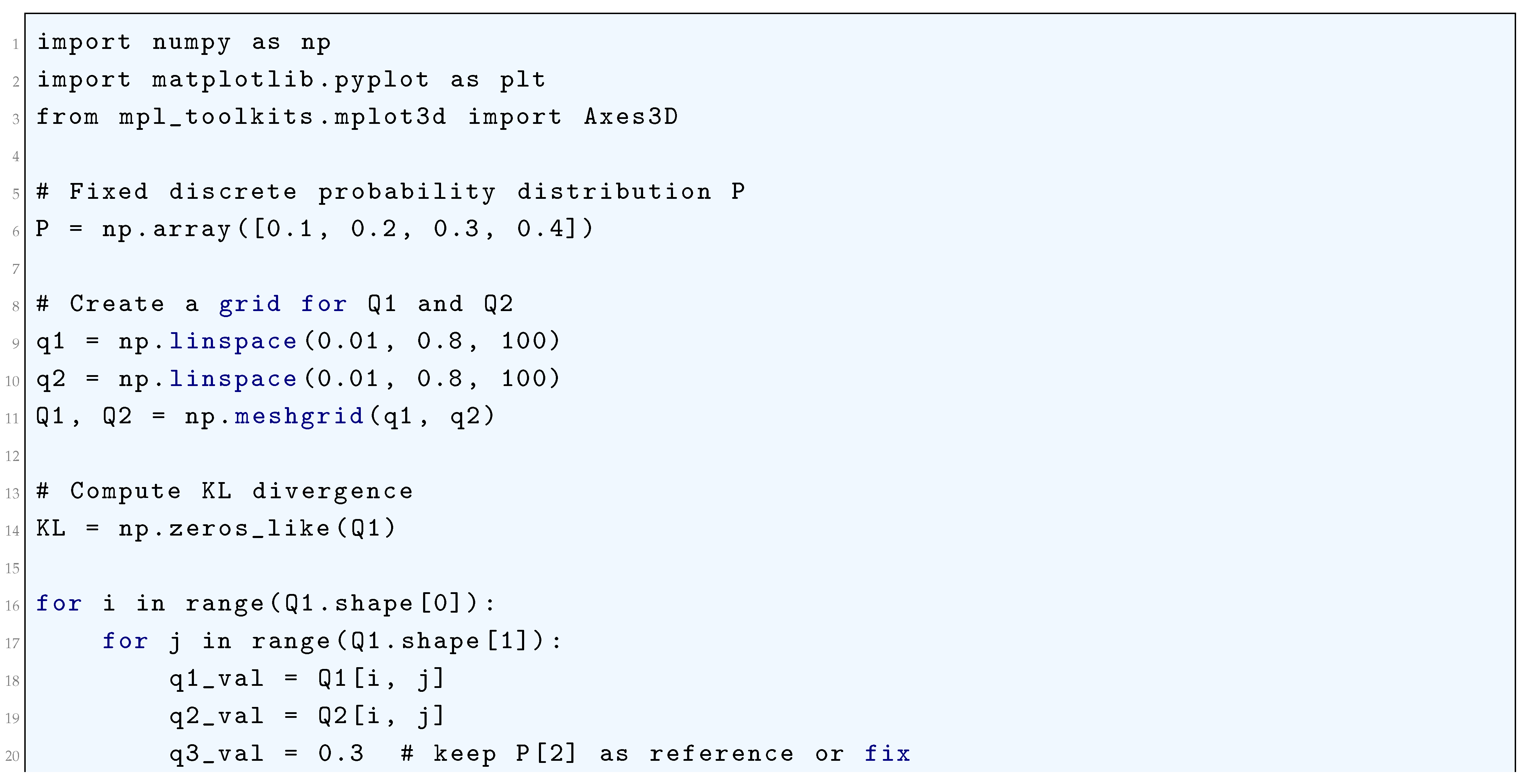
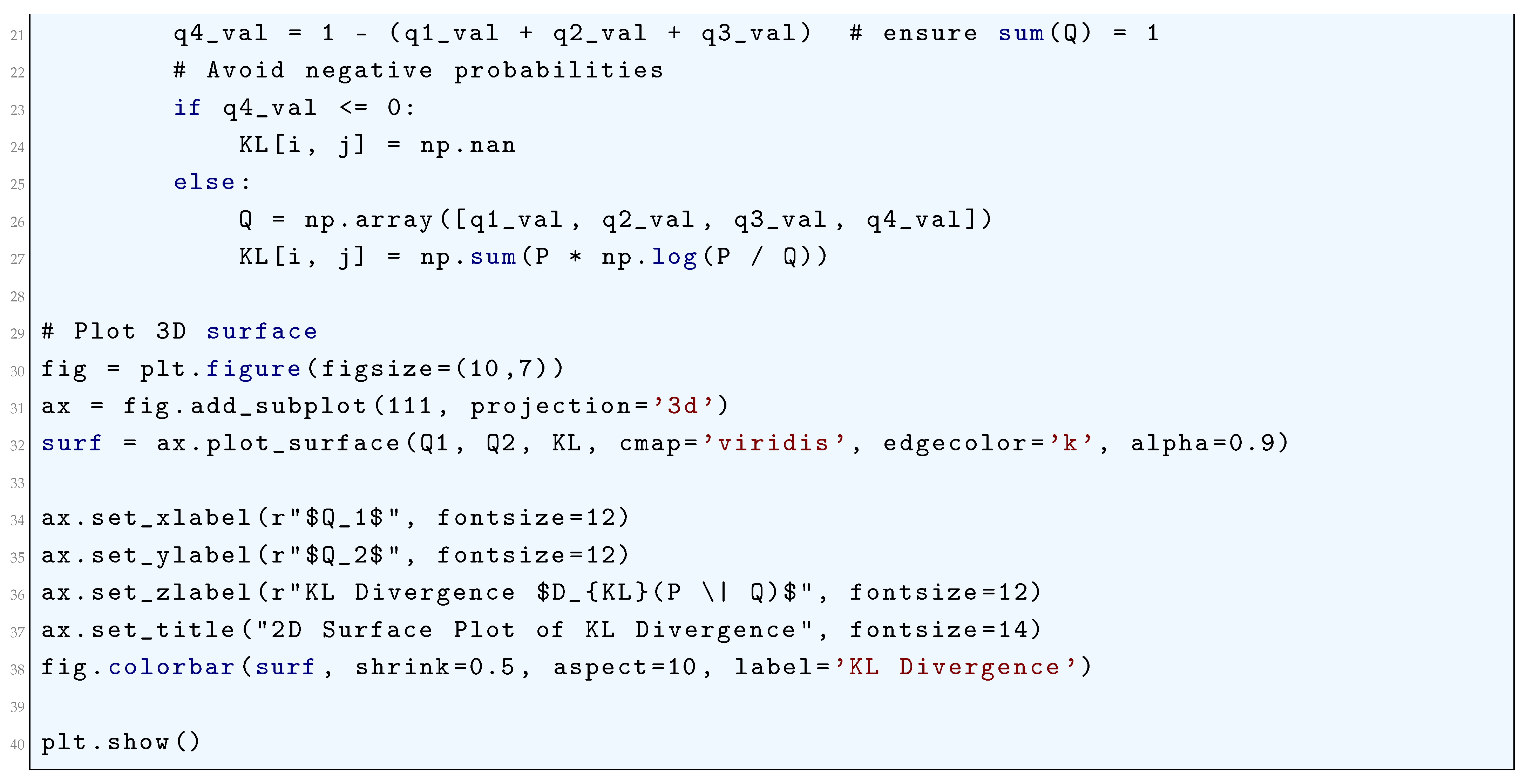
10.5.3. Advanced and Specialized Loss Functions
10.5.3.1 Loss Functions for Generative Adversarial Networks (GANs)
10.5.3.1.1 Wasserstein Loss (Earth Mover’s Distance)
The Wasserstein Loss, also known as the Earth Mover’s Distance (EMD) or Kantorovich-Rubinstein metric, is a fundamental function from optimal transport theory that provides a mathematically rigorous and continuous measure of the distance between two probability distributions. Unlike the Kullback-Leibler (KL) or Jensen-Shannon (JS) divergences, which can be undefined or exhibit vanishing gradients when the distributions have disjoint supports—a common scenario in the low-dimensional manifolds of high-dimensional data like images—the Wasserstein Distance is defined even for non-overlapping distributions and yields a smooth, meaningful gradient that is essential for stable optimization in deep learning, particularly in Generative Adversarial Networks (GANs). For two probability distributions (real data) and (generated data) defined on a metric space , the p-th Wasserstein distance is defined as the minimum cost of transporting mass from to , where the cost is taken to be the p-th power of the distance. For , which is most common in machine learning, it is given by:
Here, denotes the set of all joint distributions whose marginal distributions are and , i.e.,
and
This primal formulation directly captures the intuition of finding the most efficient transport plan that moves the probability mass from to , with the cost proportional to the distance .
Computing the infimum over all possible couplings is intractable for high-dimensional problems. However, a transformative result from duality theory, the Kantorovich-Rubinstein duality, provides a computationally feasible equivalent formulation. The duality states that:
where the supremum is taken over all 1-Lipschitz functions , meaning functions that satisfy
for all . This dual form is the foundation of the Wasserstein Loss in Wasserstein GANs (WGANs). Instead of minimizing the distance directly, one maximizes the difference in expectations between the real and generated data over a family of Lipschitz-constrained functions, represented by a critic network with parameters w. The training objective becomes a minimax game:
where is the generator mapping noise z to data space. The critic is trained to maximize this expression, effectively estimating the Wasserstein distance, while the generator is trained to minimize it by making the generated distribution indistinguishable from under the critic’s assessment.
The critical mathematical detail is the enforcement of the 1-Lipschitz constraint on the critic function . Without this constraint, the maximization could diverge to infinity, rendering the loss meaningless. Several techniques exist to enforce this constraint approximately. The original WGAN paper proposed weight clipping, constraining the weights w of the critic to a compact space , which ensures the network is K-Lipschitz for some K but can lead to pathological behavior like capacity underuse or gradient vanishing. A more effective and widely adopted method is the Gradient Penalty (WGAN-GP), which adds a regularization term to the loss that directly enforces the Lipschitz constraint on the interpolated data points. The WGAN-GP loss for the critic is:
where is a random point sampled along straight lines between points from and , i.e.,
with , , . This term penalizes the gradient norm of the critic at these points, deviating from 1, thus encouraging it to be 1-Lipschitz. The generator’s loss remains
The differentiability and continuity of the Wasserstein Loss under this formulation provide stable, linear gradients that do not saturate, even when the critic is optimal, solving the key training instability problems of traditional GANs that use JS divergence. The value of the Wasserstein Loss itself also correlates well with the perceived quality of the generated samples, making it a useful diagnostic metric during training.
10.5.3.1.2 Least Squares GAN (LSGAN) Loss
The Least Squares Generative Adversarial Network (LSGAN) loss function is a modification of the standard Generative Adversarial Network (GAN) objective that replaces the binary cross-entropy loss with a least squares term, fundamentally altering the properties of the optimization landscape to improve training stability and mitigate the vanishing gradients problem inherent in the original formulation. The core theoretical motivation stems from the observation that minimizing the Pearson divergence between the model distribution and the data distribution can be achieved through a least squares cost function, which provides smoother and more non-vanishing gradients, especially when updating the generator on samples that are on the correct side of the decision boundary but are still far from the real data manifold. In the standard GAN framework, the discriminator D (often called the critic in this context) is trained to output a probability that a sample is real, using the sigmoid activation and binary cross-entropy loss. LSGAN re-frames this: the discriminator D is now a function that assigns a real-valued score to inputs, and its objectives for real and fake data are defined by the least squares error. Specifically, for a real sample , the desired discriminator output is a, and for a generated sample where , the desired output is b, with a and b being hyperparameters typically set to . The loss functions for the discriminator D and generator G are thus formulated as:
Here, c is another hyperparameter denoting the value that the generator wants the discriminator to believe for its generated samples; a common choice is , meaning the generator aims to make its samples indistinguishable from real data by pushing their discriminator scores towards 1. The choice of these targets a, b, and c is not arbitrary; it has a theoretical basis in minimizing a specific f-divergence. The objective for the discriminator is to minimize the squared error of its predictions relative to the target labels a (real) and b (fake), effectively performing regression rather than classification. This formulation ensures that even if a generated sample is correctly classified as fake (i.e., is close to b), it still incurs a significant loss if it is far from the decision boundary, providing a strong gradient signal to the generator to improve. Conversely, in the standard GAN, a generated sample that is confidently wrong (far on the wrong side of the decision boundary) results in a saturated sigmoid and a vanishingly small gradient.
The mathematical optimality of the LSGAN can be analyzed by solving for the optimal discriminator for a fixed generator G. For any given generator, the discriminator objective is to minimize the expected squared error. Assuming the densities for real data and for generated data exist, the objective can be written as an integral over the input space:
To find the function D that minimizes this, we take the functional derivative with respect to and set it to zero:
Solving for yields the optimal discriminator:
Substituting this optimal discriminator back into the generator’s objective function reveals the quantity that the generator is ultimately minimizing. With c as the generator’s target, the generator loss becomes:
By plugging in the expression for , this loss can be shown to be proportional to the Pearson divergence between and , plus a constant, for specific choices of a, b, and c. The most common setting leads to the generator minimizing
This divergence is smoother and better behaved than the Jensen-Shannon divergence targeted by the original GAN, leading to more stable training dynamics. The gradients for the generator are given by
Since is a linear term, it does not saturate, ensuring that the generator receives a usable gradient as long as the discriminator provides a meaningful score , which it does due to the regression task. This property is the primary advantage of LSGAN: it avoids the vanishing gradient problem that plagues standard GANs when the discriminator becomes too confident, thereby facilitating more reliable convergence and often producing higher quality generated samples.
10.5.3.1.3 Adversarial Loss (Standard GAN Loss)
The Adversarial Loss, as formulated in the original Generative Adversarial Network (GAN) framework, establishes a two-player minimax game between a generator network G and a discriminator network D, where the solution is a Nash equilibrium. The generator G maps samples from a prior noise distribution (typically a multivariate Gaussian or uniform distribution) to the data space, synthesizing samples intended to resemble real data. The discriminator D is a binary classifier that outputs a probability that a given input x originates from the real data distribution rather than the generator’s distribution . The objective function for this game is given by the value function :
This formulation derives from the principle of binary cross-entropy minimization. For a fixed generator G, the optimal discriminator is the function that maximizes this expression for every x. The argument inside the expectation for the discriminator is
To find the maximizing for a fixed x, we take the functional derivative with respect to and set it to zero, yielding the condition:
Solving this equation provides the optimal discriminator for a fixed generator:
Substituting this optimal discriminator back into the value function reveals the global loss function that the generator is ultimately minimizing:
This expression can be rewritten in terms of the Kullback-Leibler (KL) divergence and the Jensen-Shannon (JS) divergence. Specifically, it equals:
where the Jensen-Shannon divergence is defined as
with
Thus, the global minimum of the generator’s loss is achieved if and only if , at which point for all x, and .
The training process involves alternating gradient-based updates for D and G. The discriminator update maximizes by ascending its stochastic gradient:
where is a minibatch from the real data and is a minibatch from the noise prior. The generator update minimizes by descending its stochastic gradient. However, in early training, when is close to zero, the gradient of vanishes, providing no learning signal. To circumvent this, practitioners often maximize
instead of minimizing
which provides stronger gradients early on, though it changes the theoretical interpretation. The gradient for this modified generator objective is:
Despite the theoretical guarantee of convergence to the true data distribution, the training of standard GANs is notoriously unstable due to several factors: the simultaneous gradient descent on a non-convex game often leads to oscillatory behavior rather than convergence to the Nash equilibrium; the supports of and may be disjoint in high-dimensional spaces, causing the JS divergence to be constant and gradients to be zero; and mode collapse can occur, where the generator maps multiple noise inputs to the same output, failing to capture the full diversity of the data distribution. The adversarial loss thus represents a foundational but practically challenging objective that has spurred numerous variants designed to stabilize training and improve performance.
10.5.3.2 Loss Functions for Siamese and Metric Learning
10.5.3.2.1 Contrastive Loss
Contrastive Loss is a distance-based loss function fundamental to metric learning and siamese network architectures, designed to learn an embedding space where similar data pairs are projected closer together while dissimilar pairs are pushed apart by a margin.
The core objective is to train a parameterized embedding function that maps input samples into a low-dimensional manifold where the Euclidean distance
directly reflects semantic similarity. For a training pair of samples , a label Y is defined where if the pair is similar (positive pair) and if dissimilar (negative pair). The loss function for a single pair is formulated as:
Here, is a hyperparameter defining the margin—the minimum distance that dissimilar pairs should maintain. The first term, , applies to positive pairs and minimizes the squared Euclidean distance between their embeddings, directly pulling them together. The second term applies to negative pairs and is active only when their distance is less than the margin m; it penalizes the pair by the squared difference between the margin and their current distance, effectively pushing them apart until their separation is at least m. This loss function encourages the embedding function to create a structured space where intra-class variance is minimized and inter-class variance is maximized, with the margin providing a buffer zone to prevent excessive contraction of the entire dataset into a single point.
The mathematical properties of Contrastive Loss reveal its optimization dynamics. The gradient with respect to the embedding vectors drives the learning process. For a positive pair , the gradient of the loss with respect to the distance d is , which is linear and pulls the embeddings together with a force proportional to their current separation. For a negative pair where , the gradient is
which pushes the embeddings apart with a force that diminishes as the distance approaches the margin. If for a negative pair, the loss is zero and no gradient is produced.
The gradients with respect to the embeddings themselves are derived through the chain rule. For a positive pair, the gradient for an embedding vector is:
For a negative pair with , the gradient is:
These gradients show that the update magnitude for positive pairs is linear in the distance, while for negative pairs it is sublinear, scaling with . This structure helps prevent catastrophic collapse where all embeddings converge to zero, as the repulsive force for negative pairs counteracts the attractive force for positive pairs. The margin m is critical; it defines the scale of the embedding space and prevents the loss from becoming trivial (e.g., all distances shrinking to zero).
The overall loss for a minibatch is typically the average over all pairs. In practice, forming pairs can lead to quadratic complexity, but mining hard negatives—focusing on negative pairs that are currently too close—can improve efficiency and performance. Contrastive Loss is a foundational objective that has been extended in numerous ways, such as in triplet loss and modern self-supervised methods like SimCLR, but its core principle of contrasting similar and dissimilar pairs remains a pillar of representation learning.
10.5.3.2.2 Triplet Loss
Triplet Loss is a metric learning objective designed to learn an embedding function that projects input data into a Euclidean space where semantically similar points are clustered and dissimilar points are separated by a distance proportional to their semantic difference.
It operates on triplets of samples: an anchor sample , a positive sample (semantically similar to the anchor, e.g., same class), and a negative sample (semantically dissimilar to the anchor, e.g., different class). The fundamental aim is to ensure that the distance between the anchor and positive is less than the distance between the anchor and negative by at least a predefined margin . Mathematically, this constraint is expressed as
and the loss for a single triplet is defined as the amount by which this inequality is violated:
This is a hinge-like loss that is zero if the embedding function successfully pushes the negative pair beyond the margin relative to the positive pair, and positive otherwise, providing a gradient to correct the embedding. The margin m acts as a hyperparameter controlling the minimum desired separation between positive and negative pairs, preventing the trivial solution where all embeddings collapse to a single point and enforcing a meaningful topology in the latent space.
The optimization dynamics of Triplet Loss are governed by the gradients with respect to the embedding vectors. Let
and
denote the Euclidean distances for the positive and negative pairs, respectively. The loss is active only when
In this case, the gradients are computed as follows. The gradient with respect to the anchor embedding is:
The gradient with respect to the positive embedding is:
The gradient with respect to the negative embedding is:
These gradients reveal that, when active, the loss pulls the anchor and positive together while pushing the anchor and negative apart. The update magnitudes are proportional to the current distances, providing a self-stabilizing effect: large violations yield large gradients, while small violations yield fine adjustments. The overall loss for a dataset is the average over all valid triplets, but sampling all possible triplets is computationally prohibitive.
Thus, hard negative mining is critical: selecting triplets where the negative is currently closer to the anchor than the positive i.e.
or semi-hard negatives where
but the loss is still positive. This focuses learning on the most informative triplets that violate the margin constraint, improving efficiency and convergence. The success of Triplet Loss hinges on the careful balance between attractive and repulsive forces, and it has been foundational for tasks like face recognition and image retrieval, where learning a discriminative embedding is paramount.
10.5.3.2.3 Center Loss
Center Loss is a supervised learning objective function designed to enhance the discriminative power of learned features by simultaneously promoting inter-class dispersion and intra-class compactness in the feature space of a deep neural network. It operates alongside a traditional softmax cross-entropy loss, which primarily encourages features to be separable by maximizing the decision boundary between different classes but does not explicitly enforce features of the same class to form tight, distinct clusters. The Center Loss addresses this by introducing a penalty term that pulls the deep features of each sample toward the center of its corresponding class, thereby reducing the intra-class variations that can impede robust classification, especially under challenging conditions like pose changes or illumination variations in face recognition.
Mathematically, for a training dataset with N samples and C classes, let be the deep feature of the i-th sample belonging to class . The Center Loss maintains a learnable center vector for each class, which is updated iteratively during training to represent the mean feature of that class. The Center Loss term for a single sample is defined as the squared Euclidean distance between the feature vector and its corresponding class center :
The complete loss function is then a weighted combination of the softmax cross-entropy loss and the Center Loss :
where is a hyperparameter that balances the two loss components, and are the weight vector and bias for class j in the final fully connected layer, and the softmax loss ensures inter-class separability.
The optimization of Center Loss involves updating both the network parameters and the class centers through backpropagation. The gradients of the total loss L with respect to the feature vector and the center are critical for training. The gradient of L with respect to is:
where is the gradient from the softmax loss, which pushes features toward the decision boundary of their class, while the Center Loss gradient pulls features toward their class center. The centers are updated based on the features of all samples in the batch belonging to class j, but to avoid large perturbations caused by misclassified samples, the update uses a scaling factor and is computed as:
where is the indicator function, and the centers are updated via
This update gradually moves each center toward the mean of its class features without being overly sensitive to mini-batch noise.
The interplay between the softmax loss and Center Loss ensures that features not only are separable but also exhibit small intra-class variance, leading to a more robust and generalized feature representation. The hyperparameter controls the trade-off: too small a weakens the intra-class compactness effect, while too large a may overwhelm the softmax loss, causing features to collapse into their centers and degrading classification performance. Center Loss has proven effective in tasks requiring high discriminative feature learning, such as face verification and fine-grained recognition, by producing features that are both highly discriminative and invariant to intra-class variations.
10.5.3.3 Loss Functions for Style Transfer and Super-Resolution
10.5.3.3.1 Perceptual Loss
Perceptual Loss is a feature-based loss function that quantifies the discrepancy between two images not in raw pixel space but in a high-dimensional feature space extracted by a pre-trained deep convolutional neural network (typically a VGG network trained on ImageNet), thereby measuring perceptual similarity rather than strict pixel-to-pixel correspondence.
This approach is grounded in the hypothesis that features learned by a network trained for a high-level task (e.g., image classification) encode semantic and perceptual information that is more aligned with human visual perception than low-level pixel errors. Given a target image y and a generated image , let denote the feature map activations from the j-th layer of a pre-trained network when processing an image x. The Perceptual Loss between y and is defined as the Euclidean distance between their feature representations at one or more layers:
where , , and are the number of channels, height, and width of the feature map at layer j, and the normalization by the spatial dimensions ensures the loss is scale-invariant across layers. By leveraging hierarchical features from multiple layers (e.g., ReLU layers from VGG-16), the loss captures both high-level semantic content (from deeper layers) and finer texture details (from shallower layers), enabling the generation of images that are perceptually realistic even if they exhibit slight geometric or photometric deviations from the target.
The mathematical rigor of Perceptual Loss arises from its interpretation as a metric in the feature manifold of a pre-trained network. The feature extractor serves as a non-linear mapping from the image space to a feature space , where distances correlate with perceptual differences. The loss assumes that has learned a sufficiently rich and disentangled representation where semantically similar images are mapped to nearby points. The gradient of the loss with respect to the generated image is computed through the pre-trained network:
where is the Jacobian of the feature map at . Since is pre-trained and fixed, these gradients guide the optimization process to adjust in directions that minimize feature-space distance, effectively transferring perceptual attributes from y to . This is particularly useful for tasks like style transfer, super-resolution, and image synthesis, where maintaining perceptual fidelity is more critical than pixel-level accuracy. However, the loss depends heavily on the choice of network and the layers j; deeper layers emphasize semantic content, while shallower layers capture spatial details. Variants of Perceptual Loss, such as using the LPIPS (Learned Perceptual Image Patch Similarity) metric, further improve by learning the feature space distance from human judgments, but the core principle remains: leveraging deep features as a perceptual metric for image comparison.
10.5.3.3.2 Style Loss
Style Loss is a specialized function used primarily in neural style transfer to quantify the difference in stylistic appearance between two images by comparing the statistical properties of their feature representations, specifically the correlations between filter responses encoded by the Gram matrix of feature activations from a pre-trained deep convolutional network. Unlike perceptual loss, which focuses on content similarity by matching feature maps directly, style loss operates on the premise that the style of an image is captured by the inter-channel correlations within feature maps, which correspond to textures, patterns, and visual motifs independent of the spatial structure.
Given a feature map activation tensor extracted from layer j of a pre-trained network (e.g., VGG-19) for an image x, the Gram matrix is computed as the inner product between the vectorized feature maps across spatial dimensions, effectively measuring the covariance between channels:
where index feature channels. This matrix is symmetric and positive semi-definite, and its elements represent the degree to which features k and l co-occur spatially in the image. The style loss between a target style image and a generated image is then defined as the mean squared error between their Gram matrices across a set of layers :
where denotes the Frobenius norm, and the normalization by accounts for the number of elements in the Gram matrix. This loss encourages the generated image to exhibit similar texture statistics to the style image by matching the second-order moments of feature distributions, effectively transferring stylistic attributes such as brushstrokes, color palettes, and patterns without preserving the spatial content.
The mathematical foundation of style loss relies on the interpretation of the Gram matrix as an estimator of the feature distribution’s covariance structure. Minimizing the Frobenius norm between Gram matrices is equivalent to minimizing the Euclidean distance between the vectorized representations of the feature correlations, which aligns the stylistic properties of the generated image with those of the target style. The gradient of the style loss with respect to the generated image is computed through the chain rule:
where involves the Jacobian of the Gram matrix computation. This gradient updates to increase or decrease specific feature correlations, effectively synthesizing textures that mimic the style image. The choice of layers is critical: shallow layers capture low-level textures (e.g., edges, colors), while deeper layers encode higher-order style patterns (e.g., complex structures). In practice, style loss is combined with content loss (e.g., perceptual loss) and often a total variation regularization term to produce visually coherent stylized images. The efficacy of style loss stems from its ability to disentangle style from content by leveraging the statistical independence of feature correlations from spatial arrangements, making it a cornerstone of artistic style transfer and texture synthesis in computer vision.
10.5.3.3.3 Total Variation (TV) Loss
Total Variation (TV) Loss is a regularization term employed in image processing and inverse problems to impose spatial smoothness on an image by penalizing excessive and spurious variations in pixel intensities, thereby reducing noise and undesired high-frequency artifacts while preserving essential edges and structures.
It is grounded in the mathematical theory of functions of bounded variation, where the total variation of a function is defined as the integral of the absolute value of its gradient, capturing the total magnitude of oscillations and discontinuities. For a discrete 2D image with height H and width W, the anisotropic Total Variation Loss is commonly defined as the sum of the absolute differences between adjacent pixels along the horizontal and vertical directions:
This formulation measures the -norm of the discrete gradients, promoting sparsity in the image gradient domain and encouraging piecewise constant regions with sharp boundaries. An alternative isotropic Total Variation Loss combines the horizontal and vertical differences using the Euclidean norm at each pixel:
which more accurately approximates the continuous total variation but is computationally more intensive due to the square root operation. The primary effect of TV Loss is to suppress small fluctuations caused by noise or artifacts while preserving significant edges, as the -norm imposes a stronger penalty on small gradients than the -norm used in quadratic smoothness terms.
The mathematical properties of TV Loss arise from its convexity and non-differentiability at zero. The gradient of the anisotropic TV Loss with respect to the image x is straightforward but requires care at points of non-differentiability. For a single pixel , the partial derivative of is:
where the `sign` function is defined in the subgradient sense at zero (typically returning 0 for a zero difference). This gradient effectively acts as a diffusion term that reduces variations between neighbors, flattening regions with small gradients while leaving large jumps unchanged. In optimization problems, such as image reconstruction or generation, TV Loss is often added as a regularization term with a weight to the primary loss function:
where ensures fidelity to observed data (e.g., mean squared error for reconstruction). The parameter controls the trade-off between smoothness and data fidelity; too large a oversmooths the image, erasing fine details, while too small a fails to suppress noise. TV Loss is particularly effective in tasks like image denoising, inpainting, and style transfer, where it helps produce visually plausible results by eliminating unstructured noise and creating piecewise smooth outputs. Its use in deep learning, such as in generative models, stabilizes training by preventing high-frequency artifacts that can arise from unconstrained optimization, ensuring that generated images adhere to natural image statistics characterized by sparse gradients.
10.5.3.4 Loss Functions for Uncertainty Estimation and Bayesian Deep Learning
10.5.3.4.1 Evidence Lower Bound (ELBO) Loss
The Evidence Lower Bound (ELBO) loss is the foundational objective function in variational inference, a method used to approximate intractable posterior distributions in probabilistic models, most prominently in Variational Autoencoders (VAEs). It derives from the principle of maximizing the log-likelihood of the observed data , which is computationally infeasible due to the integration over latent variables z. Instead, variational inference introduces an approximate posterior distribution , parameterized by , and seeks to minimize the Kullback-Leibler (KL) divergence between and the true posterior . This divergence is non-negative and satisfies:
where is the ELBO, defined as:
The ELBO provides a lower bound on the log-evidence , as the KL term is always non-negative. Maximizing the ELBO is equivalent to minimizing , thus making a better approximation of the true posterior. The first term in the ELBO, , is the reconstruction loss, which encourages the decoder to generate data that matches the observed input x. The second term, , acts as a regularizer, penalizing deviations of the approximate posterior from the prior , typically chosen as a standard Gaussian . This KL divergence term can often be computed analytically, especially when both and are Gaussian, ensuring computational efficiency.
The optimization of the ELBO involves gradient-based methods, but the expectation term poses a challenge due to the non-differentiability of sampling from . This is addressed by the reparameterization trick, which expresses the latent variable as a deterministic function of parameters and an auxiliary noise variable: with . For a Gaussian , this becomes
where . This transformation allows gradients to flow through the stochastic layer, enabling unbiased Monte Carlo estimates of the gradient:
The KL divergence term for Gaussian distributions has a closed-form expression:
where J is the dimensionality of z, and and are the parameters of . This term encourages the latent codes to remain close to the prior, preventing overfitting and promoting a structured latent space. The ELBO loss is thus:
which is minimized during training. The balance between reconstruction accuracy and latent regularization is automatic but can be tuned with a weight parameter in variants like -VAE, which uses to emphasize disentangled representations. The ELBO framework ensures tractable optimization while providing a rigorous bound on the data likelihood, making it a cornerstone of modern deep generative models.
10.5.3.4.2 Negative Log-Likelihood (NLL) Loss
Negative Log-Likelihood (NLL) Loss is a fundamental objective function in statistical estimation and machine learning that arises from the principle of maximum likelihood estimation (MLE), aiming to find the parameters of a model that make the observed data most probable.
Given a parametric model that defines the probability of data point x under parameters , and assuming independent and identically distributed (i.i.d.) data samples , the likelihood function is
Maximizing this likelihood is equivalent to minimizing the negative log-likelihood, due to the monotonicity of the logarithm function, leading to the NLL loss:
The normalization by N expresses the loss as an empirical expectation over the data distribution: , which is the cross-entropy between the true data distribution and the model distribution . Minimizing the NLL loss thus minimizes the Kullback-Leibler divergence , as
where is the entropy of the data and is constant with respect to . This establishes NLL as a direct measure of how well approximates .
In practice, for discrete outcomes such as classification, is often a categorical distribution where the model outputs a probability vector over classes. For a true label (represented as a one-hot vector) and predicted probabilities , the NLL loss for that sample is , which is the cross-entropy loss. For continuous data, such as regression, is typically a parametric distribution like a Gaussian , and the NLL loss becomes:
which couples the mean and variance terms. In heteroscedastic regression, where the variance is also predicted, minimizing NLL allows the model to learn uncertainty estimates automatically. The gradient of the NLL loss with respect to the parameters is:
which is the negative of the gradient of the log-likelihood. For exponential family distributions, this gradient has favorable properties, often leading to efficient optimization. The Hessian of the NLL loss is related to the Fisher information matrix
which characterizes the curvature of the likelihood surface and plays a key role in natural gradient methods. NLL loss is widely used in deep learning for generative modeling (e.g., VAEs, autoregressive models), classification, and probabilistic regression, providing a statistically principled way to train models that output full probability distributions rather than point estimates. Its minimization ensures consistency and efficiency under correct model specification, per the asymptotic properties of MLE.
10.5.3.5 Loss Functions for Domain Adaptation
10.5.3.5.1 Domain Adversarial Loss
Domain Adversarial Loss is a strategic objective function employed in domain adaptation to learn feature representations that are invariant across a source domain and a target domain , thereby facilitating knowledge transfer from a label-rich source to an unlabeled target.
The core idea is to train a feature extractor that produces embeddings which are indistinguishable between domains, as judged by a domain classifier that acts as an adversary. This induces a minimax game: the feature extractor aims to confuse the domain classifier, while the domain classifier strives to correctly identify the domain origin of features. Formally, let and be samples from the source and target distributions and , respectively. The feature extractor maps input x to a feature vector . The domain classifier takes f as input and outputs a probability that the feature originates from the source domain. The domain adversarial loss is then defined as the binary cross-entropy loss for the domain classifier:
where and are the number of source and target samples in the batch. The parameters of the domain classifier are optimized to minimize this loss, thus improving domain discrimination. Conversely, the parameters of the feature extractor are optimized to maximize this loss, effectively making the features domain-invariant. This adversarial dynamic is encapsulated in the overall objective:
In practice, this is achieved by gradient reversal during backpropagation: when updating , the gradient from is multiplied by (a hyperparameter) before being propagated through the feature extractor, thus implementing the maximization step.
The mathematical rigor of domain adversarial training stems from its connection to minimizing the -divergence between the source and target feature distributions. Let and be the distributions of features for and , respectively. The domain classifier aims to approximate the optimal discriminator between and , which achieves an error rate related to the Jensen-Shannon divergence. By training the feature extractor to maximize the domain classifier’s loss, it effectively minimizes the divergence between and , leading to aligned feature distributions. The overall loss for the system often combines the domain adversarial loss with a task-specific loss (e.g., classification loss on the source domain):
where denotes the parameters of a task-specific classifier (e.g., label predictor) that uses the features f, and controls the trade-off between task performance and domain invariance. The gradient updates are:
where the negative sign for on implements the gradient reversal. This framework ensures that the learned features are both discriminative for the task and invariant to domain shifts, enabling effective unsupervised domain adaptation. The success of domain adversarial loss hinges on balancing the adversary’s strength; too weak a classifier fails to align distributions, while too strong a one can overwhelm the task loss and degrade feature quality.
10.5.3.5.2 Maximum Mean Discrepancy (MMD) Loss
Maximum Mean Discrepancy (MMD) Loss is a non-parametric, kernel-based measure for comparing two probability distributions by evaluating the distance between their means in a reproducing kernel Hilbert space (RKHS), providing a rigorous framework for testing whether two samples are drawn from the same distribution without requiring density estimation.
Given two distributions P and Q over a space , and a feature map that projects samples into an RKHS with kernel
the MMD is defined as the distance between the mean embeddings and :
Using the kernel trick, this can be expressed entirely in terms of kernel evaluations:
which avoids explicit computation of the feature maps. For empirical samples and , an unbiased estimator of is:
where the sums exclude diagonal terms to avoid bias. The choice of kernel k is critical; common choices include the Gaussian kernel
where the bandwidth controls the sensitivity to multi-scale structures in the data. The MMD loss is zero if and only if when the kernel is characteristic (e.g., Gaussian), meaning the kernel map is injective, ensuring that the mean embedding captures all information about the distribution.
The mathematical properties of MMD make it particularly suitable for training generative models and domain adaptation. Minimizing MMD between the model distribution and the data distribution P provides a loss function that encourages the generator to produce samples that match the statistical properties of the real data. The gradient of the MMD loss with respect to the model parameters is:
which requires sampling from and differentiating through the kernel function. This gradient can be computed efficiently using automatic differentiation. In practice, for large datasets, minibatch estimates are used, though care must be taken with the biased estimator that includes diagonal terms when gradients are involved. The loss function is differentiable almost everywhere (for smooth kernels) and provides stable gradients, unlike adversarial losses that can suffer from vanishing gradients or mode collapse. MMD has deep connections to integral probability metrics and is equivalent to the distance between distributions under the function class induced by the kernel. Its computational complexity is , which can be prohibitive for large batches, but linear-time approximations exist, such as:
which uses non-overlapping pairs for an unbiased estimate with complexity. MMD is widely used in domain adaptation to align feature distributions between source and target domains, in generative models like MMD-GANs, and in two-sample hypothesis testing, providing a robust and statistically powerful measure of distributional similarity.
10.5.3.6 Loss Functions for Object Detection and Segmentation
10.5.3.6.1 IoU Loss (Intersection over Union) and Its Variants (GIoU, DIoU, CIoU)
The fundamental Intersection over Union (IoU) metric for two axis-aligned bounding boxes, a ground truth box A defined by its top-left and bottom-right coordinates and a predicted box B with coordinates , is calculated by first determining the coordinates of their intersection I:
The area of intersection is
The area of the union is computed from the areas of the individual boxes: , where
and
The IoU is then:
The IoU Loss is simply
The gradient of this loss with respect to a predicted coordinate, say , is found through careful application of the chain rule. The derivative is non-zero only if the boxes intersect :
Since
and is itself a piecewise function:
This complexity and the zero gradient for non-overlapping boxes motivated the development of improved variants. Generalized IoU (GIoU) Loss introduces a convex enclosure C, the smallest box containing both A and B, with coordinates:
The area of C is . GIoU is defined as:
The GIoU Loss is . Its gradient provides a signal even for non-overlapping boxes. The derivative with respect to a coordinate incorporates the new term:
The derivative is non-zero only if is the left-most point:
This guides the predicted box to expand towards the enclosure. Distance IoU (DIoU) Loss incorporates a penalty on the normalized distance between the box centers. Let the center points be
and
The Euclidean distance between centers is
Let c be the diagonal length of the enclosure C:
DIoU is defined as:
The DIoU Loss is
Its gradient includes a term that directly minimizes the center distance:
The derivative of the center distance with respect to the coordinate is:
assuming the prediction affects the center point . The derivative of the diagonal length c is:
Complete IoU (CIoU) Loss builds upon DIoU by adding an aspect ratio penalty term. It introduces a measure v to quantify the aspect ratio consistency:
where and are the width and height of the ground truth and predicted boxes, respectively. A trade-off parameter is defined as
CIoU is then:
The CIoU Loss is
Its gradient is the most complex, requiring the derivative of the aspect ratio term v with respect to the box dimensions. The gradient with respect to the predicted width is:
Similarly, the gradient with respect to the height is:
These gradients are then propagated back to the coordinate parameters through the relationships
and
for example
This comprehensive penalty ensures convergence not only in overlap and center alignment but also in the shape of the predicted bounding box, leading to superior regression accuracy.
The careful derivation of these gradients is essential for their implementation in deep learning frameworks using automatic differentiation.
10.5.3.6.2 Dice Loss
Dice Loss is a region-based loss function originating from the Sørensen–Dice coefficient, a statistical metric used to gauge the similarity between two sets. In the context of image segmentation, it measures the overlap between the predicted segmentation mask P and the ground truth mask G, making it particularly effective for tasks characterized by severe class imbalance, such as medical image segmentation where the object of interest often occupies a small fraction of the image. The Dice coefficient for binary segmentation is defined as:
where N is the total number of pixels, is the predicted probability that pixel i belongs to the foreground class, and is the corresponding ground truth label.
The Dice Loss is then formulated as
which directly minimizes the dissimilarity between the predicted and true regions. To ensure numerical stability and avoid division by zero, especially when both masks are empty, a smooth term (typically 1) is added to both the numerator and denominator:
This loss function is differentiable and can be optimized using gradient-based methods. The gradient of the Dice Loss with respect to the predicted probability at a specific pixel j is crucial for backpropagation and is given by:
This gradient indicates that the update for each pixel is influenced by the global statistics of the entire mask—specifically, the sums over all pixels—rather than just the local error. This property makes Dice Loss inherently global and particularly sensitive to the overall structure of the segmentations, providing a strong gradient signal even when the foreground region is small.
The mathematical formulation of Dice Loss can be extended to multi-class segmentation problems using a one-hot encoded representation for C classes. For each class c, the loss is computed separately and then averaged, leading to:
where is the predicted probability that pixel i belongs to class c, and is the corresponding ground truth indicator. In practice, Dice Loss is often combined with other loss functions, such as cross-entropy, to form a composite objective that leverages both region-based and distribution-based optimization. The combined loss
helps to balance the emphasis on pixel-wise accuracy and overall region overlap, often leading to improved performance and more stable convergence. The hyperparameter controls the contribution of the Dice term. From a computational perspective, the sums over all pixels make the loss efficient to compute using tensor operations, and its differentiability allows for seamless integration into deep learning frameworks. The Dice coefficient’s equivalence to the F1 score, a harmonic mean of precision and recall, underscores its suitability for scenarios where both false positives and false negatives are critical, as it naturally balances these two metrics without requiring explicit weighting.
10.5.3.6.3 Focal Loss
Focal Loss is a dynamically scaled cross-entropy loss function designed to address the extreme foreground-background class imbalance prevalent in one-stage object detection models, such as RetinaNet, by systematically reducing the relative loss contribution from well-classified examples and focusing training on hard, misclassified examples. The loss is a modification of the standard binary cross-entropy (BCE) loss for binary classification, defined for a true label and a model-estimated probability for the class with label . To notational convenience, we define as the model’s estimated probability for the true class:
The standard binary cross-entropy loss is then
The fundamental innovation of Focal Loss is the introduction of a modulating factor , where is a tunable focusing parameter, and a weighting factor for the class , with the weight for being . The complete formulation of Focal Loss is
The modulating factor is the core component that dictates the dynamic scaling; for a well-classified example where , this factor approaches 0, thus down-weighting the loss contribution for that example. Conversely, for a misclassified example where , the modulating factor approaches 1, and the loss is largely unaffected. The rate of this down-weighting is controlled by ; higher values of (e.g., ) further suppress the loss from easy examples, intensifying the focus on hard negatives. The factor is a static weight used to address class imbalance by increasing the importance of the rare class (e.g., foreground) in the loss; it can be set inversely proportional to the class frequency.
The mathematical properties of Focal Loss are critical to its efficacy. The loss function is continuous and differentiable almost everywhere, which is essential for gradient-based optimization. The gradient of Focal Loss with respect to the model’s output logit z (where ) reveals its behavior during training. The gradient is given by:
This can be simplified, considering the definition of , to:
A more intuitive understanding emerges when considering the case of a positive example (), where the gradient magnitude is proportional to .
This shows that the gradient signal diminishes for easy examples (high ) and remains significant for hard examples (low ), directly addressing the class imbalance issue where the vast number of easy negative examples would otherwise dominate the gradient. The loss is convex for a given value of , but the dynamic scaling makes the overall optimization landscape more complex, requiring careful tuning of the learning rate. The hyperparameter smoothly interpolates the loss behavior; when , Focal Loss is equivalent to -balanced cross-entropy, and as increases, the effect of the modulating factor becomes more pronounced. The parameter helps to counter the implicit weighting introduced by , which can suppress the loss for the rare class if its examples are initially easy; setting higher for the rare class ensures it continues to receive sufficient learning signal. In practice, the combined effect of and drastically improves the precision-recall trade-off on imbalanced datasets, allowing one-stage detectors to surpass the performance of more complex two-stage architectures by efficiently harnessing a much larger and more diverse set of candidate proposals during training, whose gradients are no longer drowned out by a sea of trivial background examples.
10.5.3.7 Loss Functions for Knowledge Distillation
10.5.3.8 Loss Functions for Reinforcement Learning
10.5.3.8.1 Hinge Loss
The Hinge Loss function is a convex relaxation of the 0-1 loss primarily employed for maximum-margin classification, most notably in Support Vector Machines (SVMs) but also applicable to neural networks.
Its objective is not to produce probability estimates but to find a decision boundary that maximizes the geometric margin between classes, thereby enhancing the model’s generalization capability. For a binary classification task with true labels and a model that produces real-valued scores (where is the weight vector and b is the bias), the Hinge Loss for a single data point is defined as
This piecewise function is zero if , meaning the prediction is correct and lies beyond the margin boundary, and increases linearly for .
The term is known as the functional margin; a positive value indicates a correct classification, and its magnitude represents the confidence of the prediction. The loss explicitly penalizes predictions that are either incorrect or correct but within the margin boundary (where ), with the penalty proportional to the degree of margin violation. The aggregate loss over a dataset of N samples is typically given by
where the regularization term is not merely a technical addition but is fundamental to the maximum-margin principle, directly controlling the trade-off between maximizing the margin and minimizing classification error.
From an optimization perspective, the Hinge Loss is convex and piecewise linear, which allows for efficient training using subgradient methods. Its subgradient with respect to the model’s parameters is central to learning. For a single data point, the subdifferential is:
In practice, at the point of non-differentiability , a common convention is to choose a subgradient of 0, treating the point as part of the flat region. The overall subgradient of the regularized objective L with respect to is therefore
This leads to a simple and intuitive update rule: for samples that violate the margin , the update is
(if using a subgradient of ), where is the learning rate, which pushes the decision boundary to correctly classify the sample, while the regularization term shrinks the weights. Samples outside the margin do not contribute to the weight update. This sparsity in the gradient contribution is a key property, as it means the final classifier is only defined by a subset of critical training examples—the support vectors—which are the samples that lie on or within the margin .
The Hinge Loss can be generalized to multi-class classification, known as the Crammer-Singer loss or multi-class Hinge Loss. For a problem with K classes, where the true label for a sample is an integer and the model produces a score vector , the loss is defined as
This formulation penalizes the model if the score for the correct class is not greater by at least a margin of 1 than the maximum score among all incorrect classes. The subgradient for this loss involves the incorrect class that achieves the maximum score
leading to updates that increase the score for the correct class and decrease the score for this most offending incorrect class. The Hinge Loss’s primary strength is its focus on the geometric structure of the problem, promoting robust classifiers with good generalization bounds derived from statistical learning theory, such as the Vapnik-Chervonenkis (VC) dimension and Rademacher complexity, which directly relate to the concept of the margin. Its main limitation is its lack of inherent probabilistic calibration, as it outputs a decision function rather than a probability, though methods like Platt scaling can be applied post-hoc to address this.
10.5.3.8.2 Value Loss
Value Loss, in the context of reinforcement learning (RL) and particularly actor-critic methods, is a objective function designed to train the value function estimator , parameterized by , to accurately predict the expected cumulative return from a given state s.
The value function represents the expected return when starting from state s and following policy :
where is the discount factor and is the reward at time t. The Value Loss is typically defined as the mean squared error (MSE) between the predicted value and a target value estimate , which is derived from empirical returns or bootstrapped estimates. In the Monte Carlo approach, the target is the actual return
leading to the loss
However, due to the high variance of , temporal difference (TD) methods are preferred, where the target is the bootstrapped estimate
using parameters from a previous iteration to enhance stability. The loss becomes:
where is the state distribution under policy . In advanced algorithms like Proximal Policy Optimization (PPO) and Generalized Advantage Estimation (GAE), the value loss is minimized concurrently with the policy loss to reduce variance and accelerate learning. The gradient of the value loss with respect to the parameters is:
which adjusts to minimize the TD error
To prevent overfitting and ensure training stability, the value loss is often clipped or regularized. For instance, in PPO, the value function is trained via multiple epochs on the same data, and the loss may include a clipping term or a entropy bonus. The objective becomes:
though this is less common than the policy clipping.
Alternatively, a squared error loss with a penalty on the divergence from the previous value function can be used:
where is a hyperparameter. The target can be computed using GAE, which provides a low-variance estimate of the advantage function by exponentially averaging TD errors of different steps:
where
is the GAE estimate, with controlling the bias-variance trade-off. The value loss is then:
This formulation ensures that the value function learns to approximate the true value function , which is critical for accurate advantage estimation and effective policy updates. The optimization of the value loss is typically performed using stochastic gradient descent, with gradients computed over minibatches of trajectories to ensure computational efficiency and convergence. The value function’s accuracy directly influences the policy gradient estimates, as the advantage is used to scale the policy updates, making the value loss a cornerstone of stable and efficient reinforcement learning.
10.5.3.8.3 Policy Loss
Policy Loss is the objective function used to optimize the policy in reinforcement learning, where represents the parameters of a neural network that maps states s to a probability distribution over actions a. The fundamental goal is to maximize the expected cumulative reward
where is a trajectory and is the discount factor. The policy gradient theorem provides the foundation for the policy loss by giving the gradient of this objective:
where
is the advantage function, measuring how much better action is compared to the average action in state . The basic policy loss is then formulated as the negative of the objective to be minimized:
where is an estimate of the advantage. However, this vanilla policy gradient can lead to unstable updates with high variance.
To address stability issues, Proximal Policy Optimization (PPO) introduces a clipped surrogate objective that prevents excessively large policy updates. Let
be the probability ratio between the new and old policies. The unclipped objective is
where CPI denotes conservative policy iteration. PPO modifies this by clipping the probability ratio to remain near 1, forming the primary policy loss:
where is a hyperparameter, typically 0.1 or 0.2. The clip function restricts to the interval , ensuring the policy update does not change too radically.
The min operator ensures the objective is a lower bound (pessimistic clip) on the unclipped objective, preventing the policy from being improved excessively when the advantage is positive and from being degraded too much when the advantage is negative. The gradient of this loss with respect to requires careful computation of the derivatives of the probability ratio. For a positive advantage , the gradient is
which becomes if , and 0 otherwise. For a negative advantage , the gradient is
which becomes if , and 0 otherwise. This clipping mechanism effectively removes the incentive for moving outside of the interval .
An alternative PPO objective combines the clipped surrogate with a penalty on the KL divergence between the new and old policies:
where is an adaptive coefficient. The KL divergence for categorical policies is
and its gradient encourages the new policy to not deviate too far from the old policy in terms of action distribution. The complete PPO objective often includes a value function error term and an entropy bonus for exploration, leading to the total loss:
where are coefficients, is the value loss, and is the entropy. The policy gradient can be computed using the likelihood ratio trick:
allowing for efficient estimation from trajectories. For continuous action spaces, where the policy is often a Gaussian distribution
the log probability is
and its gradient with respect to involves the derivatives of the mean and standard deviation networks. The policy loss thus provides a mathematically grounded mechanism for incrementally improving the policy while maintaining training stability through constraints on the policy change.
10.5.3.8.4 Entropy Regularization
Entropy Regularization is a technique employed in reinforcement learning, particularly in policy optimization methods like Proximal Policy Optimization (PPO) and Soft Actor-Critic (SAC), to encourage exploration by penalizing low entropy in the policy distribution, thereby preventing premature convergence to suboptimal deterministic policies.
The entropy of a discrete probability distribution is defined as
which measures the uncertainty or randomness in the action selection; maximum entropy is achieved by the uniform distribution where all actions are equally likely, while minimum entropy (zero) corresponds to a deterministic policy. In the context of the maximum entropy reinforcement learning framework, the standard objective of maximizing the expected cumulative reward is augmented with an entropy term to form a modified objective
where is a temperature parameter that controls the relative importance of entropy versus reward. The policy loss function then incorporates entropy regularization as a negative term to be maximized (or a positive term to be minimized when framed as a loss), leading to
where is the advantage estimate. The gradient of the entropy term with respect to the policy parameters is
which can be computed efficiently using automatic differentiation.
For continuous action spaces where the policy is parameterized as a Gaussian distribution
the entropy has a closed-form expression. For a multivariate Gaussian with diagonal covariance
the entropy is
The gradient of this entropy with respect to the standard deviation parameters is straightforward:
which provides a clear signal to increase the standard deviations, thereby increasing exploration.
In practice, the temperature parameter can be treated as a hyperparameter or adapted dynamically during training to maintain a target entropy level , often set as the negative dimension of the action space
The loss for the temperature parameter is
and its gradient
adjusts to balance the entropy penalty. The inclusion of entropy regularization alters the optimal policy to a softmax form:
where is the soft Q-function that includes entropy bonuses. This results in a policy that not only seeks high rewards but also maintains stochasticity, which improves exploration and robustness by preventing the policy from becoming too confident too early. The mathematical effect of entropy regularization is to smooth the optimization landscape, making gradient estimates more reliable and reducing the likelihood of getting trapped in local optima, which is crucial for solving complex environments with sparse rewards.
10.5.3.9 Loss Functions for Sparse and Structured Outputs
10.5.3.9.1 Kullback-Leibler (KL) Divergence Loss (as a Sparsity Constraint)
The utilization of Kullback-Leibler (KL) Divergence as a sparsity constraint is a Bayesian regularization technique that forces the empirical distribution of activations within a neural network layer, typically a hidden layer of an autoencoder, to approximate a pre-specified sparse prior distribution.
This method induces a form of representational sparsity, where only a small fraction of units are significantly active for any given input, thereby learning efficient, distributed codes. The core mathematical object is the KL divergence between two Bernoulli distributions: a target sparse prior with a very low mean activation probability (e.g., ), and the empirical average activation of a particular hidden unit j over a batch of m training examples. For a single unit, the average activation is
where
is the activation of unit j for input , and f is a sigmoidal activation function. The KL divergence for a Bernoulli distribution, which measures the inefficiency of assuming the distribution when the true distribution is , is given by:
This function has the desired properties of a sparsity penalty: it is zero if and only if , and it increases asymmetrically as deviates from . The asymmetry is crucial; it penalizes units that are too active more heavily than units that are not active enough , although the term for still provides a pulling force towards the target. The total sparsity penalty for a hidden layer with s units is the sum of the KL divergences over all units: .
This penalty term is then added to the primary objective function, such as the reconstruction error of an autoencoder, scaled by a sparsity regularization parameter . The complete loss function for a sparse autoencoder becomes:
The gradient of this composite loss with respect to the network’s parameters must be computed for backpropagation. The gradient of the KL penalty term with respect to the average activation is:
This gradient indicates the direction to push to minimize the penalty. Since is not a direct parameter but a function of the activations , the chain rule is applied.
The gradient of the total loss J with respect to the activation of unit j for a single example i receives an additional contribution from the sparsity penalty:
Given that
the derivative
Therefore, the sparsity-induced gradient for a single training example is effectively
This term is then propagated backwards through the activation function to update the weights and biases . For a sigmoid activation , the gradient with respect to the pre-activation is
This mechanism ensures that the learning process not only minimizes reconstruction error but also adjusts the parameters to drive the average activations of the hidden units towards the desired sparse target , resulting in a model that discovers statistically significant features in the data without over-representing them.
10.5.3.9.2 Structured Support Vector Machine (SSVM) Loss
The Structured Support Vector Machine (SSVM) loss, also known as the max-margin Markov network loss or structured hinge loss, is a convex objective function for training models that predict complex, interdependent output structures from an input , where is a discrete but exponentially large space (e.g., all possible sequences, sparse trees, or segmentations).
The fundamental principle is a generalization of the binary SVM margin principle to structured outputs: the score
of the correct output structure should be greater than the score of any other structure by a margin that scales with the loss incurred by predicting instead of . Here, is a joint feature map that encodes the compatibility between input and output , and are the model parameters. The structured hinge loss for a single training example is formulated as:
where is a task-specific cost function that quantifies the discrepancy between the true structure and a candidate structure ; it is zero if and positive otherwise. The maximization over , often called the "loss-augmented inference" problem, finds the most violating incorrect structure—the one that has a high score according to the current model and also incurs a high cost . The complete objective function for the SSVM, including regularization, is:
This objective is convex in because it is a sum of a convex quadratic function and maxima of affine functions of .
The optimization of this loss is typically performed using subgradient methods. The subgradient of the loss with respect to is given by the difference between the feature vector of the maximally violating structure and the feature vector of the true structure:
where
This subgradient indicates the direction to adjust to increase the score gap between the true structure and the most offending incorrect structure.
The critical computational challenge is solving this loss-augmented inference problem efficiently. For many structured problems where the cost function decomposes additively over the output structure (e.g., Hamming loss over sequences), and the feature map factorizes according to a graphical model (e.g., a chain or tree), dynamic programming algorithms like the Viterbi algorithm or belief propagation can compute exactly and efficiently. The overall training algorithm involves iterating over examples, solving for for each, and updating the weights via
where is a learning rate. A common alternative is the margin-rescaled formulation presented above; another is the slack-rescaled formulation, which scales the margin by the cost:
The SSVM framework provides a principled, margin-based approach to structured prediction with strong theoretical guarantees, but its efficacy hinges on the tractability of the loss-augmented inference problem and the design of a meaningful feature map that captures the input-output relationships.
10.5.3.9.3 Conditional Random Field (CRF) Loss
The Conditional Random Field (CRF) loss function is derived from the principle of maximum likelihood estimation for conditional probabilistic graphical models, specifically designed for structured prediction tasks where the output variables exhibit mutual dependencies given an input sequence .
A CRF directly models the conditional probability without making independence assumptions among the output variables , unlike generative models like Hidden Markov Models. For a linear-chain CRF, which is common in sequence labeling, the probability distribution is defined by a Gibbs distribution:
where is a feature vector capturing the association between input and label at position t (unary potential), is a feature vector capturing the transition between adjacent labels and (pairwise potential), are the model parameters to be learned, and is the partition function ensuring normalization:
The summation over all possible label sequences makes direct computation intractable for long sequences, but the chain structure allows efficient calculation using the forward-backward algorithm. The CRF loss for a training dataset is the negative conditional log-likelihood:
Minimizing this loss maximizes the likelihood of the true label sequences under the model. The gradient of the loss with respect to the parameters reveals a crucial contrast between the empirical counts and the model’s expected counts. The gradient for the unary parameters is:
and for the pairwise parameters :
The first term in each gradient is the empirical feature count from the training data, and the second term is the expected feature count under the current model distribution .
These marginal probabilities and are computed efficiently using the forward-backward algorithm, which leverages the Markov property to perform dynamic programming. The forward algorithm calculates
the probability of being in state y at time t given the observations up to t, recursively:
The backward algorithm similarly calculates
Therefore we have
The partition function is obtained as
The marginal probability for a single label is
and for two consecutive labels is
Optimization of the CRF loss is typically performed using iterative gradient-based methods like L-BFGS or stochastic gradient descent.
The convexity of the negative log-likelihood ensures convergence to a global optimum, and regularization is often added to the loss to prevent overfitting:
The CRF loss effectively captures dependencies between output labels, making it superior to independent classifiers for structured tasks like named entity recognition and part-of-speech tagging.
10.5.3.9.4 Connectionist Temporal Classification (CTC) Loss
Connectionist Temporal Classification (CTC) loss is a objective function designed for sequence-to-sequence learning tasks where the alignment between the input sequence
and the target sequence
is unknown and , commonly encountered in speech recognition and handwriting recognition.
The fundamental challenge is that the same target label sequence can be generated by multiple, variable-length alignments between the input and output. CTC addresses this by introducing a latent alignment path
where each belongs to an extended alphabet
which includes the original labels L plus a special blank symbol (denoted here as "−"). The blank symbol represents no label emission and is crucial for handling repetitions and variable timing. The conditional probability of a path given the input sequence is factorized as a product of independent probabilities at each time step, which are output by a recurrent neural network with a softmax layer over :
where is the probability of emitting symbol at time t.
A many-to-one mapping function , known as the CTC collapse function, is defined to remove all blank symbols and then merge consecutive duplicate symbols. For example,
The total probability of a given label sequence is the sum of the probabilities of all paths that map to it under :
The CTC loss function for a training example is the negative log-likelihood of this probability:
The central computational problem is efficiently calculating the sum over the exponentially large number of paths in . This is solved using a dynamic programming algorithm analogous to the forward-backward algorithm in Hidden Markov Models, known as the CTC forward-backward algorithm.
The algorithm operates on a modified label sequence of length , which is created by inserting blank symbols at the beginning, end, and between every pair of labels in . For example, if , then . This ensures that valid paths can transition between labels only via a blank. Let the forward variable be the total probability of all valid paths of length t that map to the first symbols of (where s is an index in ). The recurrence relation for is complex due to the rules imposed by : a path can only extend by staying on the same label, moving to the next label, or inserting a blank between non-repeating labels. The recurrence is:
where the indicator function allows the transition if it conforms to the collapse rules (e.g., skipping a blank or a non-repeating label). The initial conditions are and , with all others zero. The total probability is then the sum of the forward variables at the final time step for the last two nodes of :
Similarly, a backward variable is defined as the probability of all paths starting from time t and position s in to the end, and it is computed backwards from T to 1.
The gradient of the CTC loss with respect to the network outputs is essential for backpropagation. It can be expressed using the forward and backward variables:
The derivative is the sum of the probabilities of all paths that go through the symbol k at time t, which is computed as , where is the set of indices s in for which . This yields the final gradient:
This gradient is then propagated back through the softmax layer to update the network weights. The CTC loss elegantly handles the alignment problem without pre-segmented data, making it a cornerstone of modern sequence-to-sequence models.
Its main limitation is the conditional independence assumption between output frames, which more advanced models like RNN-Transducers aim to address.
10.5.3.9.5 Maximum Margin Markov Networks Loss
Maximum Margin Markov Networks (M³N) loss is a structured prediction objective that integrates the max-margin principle of Support Vector Machines (SVMs) with the probabilistic graphical model framework of Markov networks, providing a convex optimization formulation for learning discriminative models over interdependent output variables.
The core idea is to ensure that the score assigned to the correct output structure is greater than the score of any other structure by a margin that scales with the dissimilarity between them, as measured by a task-specific loss function . The score of a structure is defined linearly as
where is a joint feature mapping that decomposes over the cliques of the Markov network. For a pairwise Markov network, this decomposition is
where and are feature functions for nodes and edges respectively, and is the set of edges in the graph. The M³N loss for a single example is formulated as the structured hinge loss:
This loss is zero if the margin constraint
holds for all , and positive otherwise. The complete regularized objective function is:
where are slack variables allowing soft margins and C is a regularization parameter.
This formulation has an exponentially large number of constraints, but it can be optimized using the cutting-plane algorithm, which iteratively adds the most violated constraint for each training example. The most violated constraint for example i is found by solving the loss-augmented inference problem:
The key computational requirement is that this maximization must be tractable. When the loss function decomposes additively over the graph structure (e.g., Hamming loss), and the feature mapping decomposes over the same cliques, dynamic programming or graph cuts can be used for efficient exact inference.
The dual formulation of the M³N objective provides insight into the representation of the solution. The dual problem involves maximizing a concave objective over dual variables for each example i and each structure :
subject to . The optimal weight vector is given by
The Karush-Kuhn-Tucker (KKT) conditions for optimality require that only for structures that achieve the maximum in the loss-augmented inference problem for example i, meaning the solution is sparse and only supported by a small set of "active" structures. The gradient of the primal loss with respect to is a subgradient:
which can be used in subgradient descent optimization. The M³N framework generalizes multiclass SVMs and provides a principled way to incorporate structural dependencies into max-margin learning, with strong theoretical guarantees on generalization error.
However, its practical applicability depends critically on the ability to solve the loss-augmented inference problem efficiently, which restricts its use to structures where exact inference is feasible, such as sequences, trees, or graphs with low treewidth. The margin rescaling approach in M³N can be contrasted with slack rescaling, which uses constraints of the form
but margin rescaling is more commonly used due to its more straightforward integration with efficient inference algorithms.
10.5.3.9.6 Listwise Ranking Losses
Listwise ranking losses are a class of objective functions designed for learning to rank by directly modeling the probability distribution over the entire permutation of items in a list, thereby optimizing the global ordering rather than focusing on independent pairwise comparisons. The fundamental principle is to define a mapping from the predicted scores of items, assigned by a model , to a probability distribution over all possible permutations of those items, and then to minimize the discrepancy between this predicted distribution and the idealized distribution derived from the ground truth ranking. The ground truth is typically represented as a set of relevance scores for a list of n items associated with a query. The ListNet framework, a prominent listwise approach, utilizes the Plackett-Luce model to define the probability of a particular permutation of the indices . According to this model, the probability of a permutation is given by the product of sequential conditional probabilities:
where are the predicted scores from the model, , and denotes the item placed at the j-th position in the permutation. This model captures the notion that the probability of an item being ranked first is proportional to the exponential of its score, and subsequent positions are determined by repeatedly applying the same logic to the remaining items.
The ground truth distribution is often not a full permutation but a set of relevance labels. To handle this, the top-one probability is used as a surrogate. The top-one probability for item i is the probability that it is ranked first under the Plackett-Luce model:
Similarly, the ground truth top-one probability is defined using the actual relevance scores:
where is a transformation function, typically chosen as an exponential function to maintain a softmax form, or a linear function for simplicity. The loss function for a single query is then defined as the cross-entropy between the two top-one probability distributions over the n items:
If is the exponential function, this simplifies to:
The gradient of this loss with respect to the predicted score of a single item is:
This gradient has an elegant interpretation: it is the difference between the predicted probability that item j is the most relevant and the ground truth probability. This gradient is then backpropagated through the scoring function to update the model parameters . The loss function is convex in the scores , and the optimization process effectively pushes the predicted score distribution to match the ground truth relevance distribution.
A more direct but computationally intensive listwise loss is the likelihood loss, which aims to maximize the probability of the optimal permutation. If the ground truth is a full ordering , the loss is the negative log-likelihood under the Plackett-Luce model:
The gradient of this loss for a score involves a sum over all positions in the permutation where the item appears and all items that were ranked below it, making it more complex than the top-one approximation. Listwise losses are considered superior to pairwise and pointwise losses in information retrieval because they directly optimize the entire list structure, which is the ultimate goal of ranking.
However, their computational cost is higher due to the need to compute the normalization term over all items for each query, and they require meaningful ground truth relevance scores rather than just binary preferences. The mathematical rigor of listwise approaches lies in their direct formulation as probabilistic models of permutation, providing a principled foundation for learning ranking functions that perform well on metrics like Normalized Discounted Cumulative Gain (NDCG).
10.5.3.9.7 Pairwise Ranking Losses
Pairwise ranking losses constitute a fundamental family of objective functions in metric learning and information retrieval, operating on the principle of comparing pairs of items to learn a representation or scoring function that imposes a desired ordinal structure on the data. The core objective is to ensure that for a given anchor instance , the distance to a positive (similar) instance is smaller than the distance to a negative (dissimilar) instance by at least a specified margin. Let be an embedding function parameterized by that maps an input x to a vector in , and let be a distance metric, typically the Euclidean distance . The generalized pairwise hinge loss, or margin ranking loss, for a triplet is defined as:
where is the margin hyperparameter.
This loss is zero if the negative instance is already more distant from the anchor than the positive instance by at least the margin m, and increases linearly with the violation otherwise. The gradient of this loss with respect to the embedding vectors drives the learning process. When the loss is active
The gradients are:
where
and
These gradients pull the anchor and positive together while pushing the anchor and negative apart, with forces inversely proportional to their current distances, providing a stable optimization landscape.
A more probabilistic formulation is provided by the Bayesian Personalized Ranking (BPR) loss, which is derived from a maximum posterior estimator for implicit feedback data. The BPR objective maximizes the probability that a user prefers a positive item over a negative item . The probability is modeled by a sigmoid function over the difference of their scores:
where is a scoring function. The BPR loss for a triplet is the negative log-likelihood:
This is a smooth approximation of the hinge loss. Its gradient with respect to the score difference is:
which provides a well-defined, non-zero gradient for all inputs. The gradients with respect to the model parameters are then computed via the chain rule based on the specific form of .
For a scoring function based on Euclidean distance in an embedding space, where
the BPR loss encourages the distance between the user and the positive item to be less than the distance to the negative item. The gradient computations become analogous to the margin ranking loss but with a weighting factor from the sigmoid derivative. The overall objective for a dataset is the sum over all valid triplets , which can be sampled from the observed interactions. The optimization of pairwise ranking losses is efficient because it scales with the number of pairs rather than the full list, but it requires careful sampling of informative triplets. Hard negative mining, which selects negative instances that are currently close to the anchor, is critical for efficient learning and high model performance. The mathematical rigor of pairwise losses lies in their direct optimization of the relative order between items, which aligns with ranking metrics more closely than pointwise approaches, while remaining computationally more tractable than full listwise methods.
10.5.3.9.8 Contrastive Divergence (CD) Loss
Contrastive Divergence (CD) loss is an approximate maximum likelihood learning algorithm for energy-based probabilistic models, most notably Restricted Boltzmann Machines (RBMs), which provides an efficient method to estimate the gradient of the log-likelihood function without requiring intractable computations over the entire model distribution.
The core challenge in training an RBM with parameters —where is the weight matrix between visible units and hidden units , and , are bias vectors—is that the log-likelihood gradient for a single training datum involves an expectation over the model distribution :
The first term, the positive phase, is tractable as it requires averaging over the conditional distribution , which factorizes due to the bipartite structure of the RBM. The second term, the negative phase, is an expectation over the joint model distribution and is computationally prohibitive as it sums over all possible configurations of and . Contrastive Divergence approximates this negative phase expectation by starting from the data point and running a short Markov Chain Monte Carlo (MCMC) simulation for k steps (typically ), rather than running the chain to convergence.
The CD-k algorithm proceeds as follows. First, given a training sample , sample a hidden state from the conditional distribution:
For binary units, this is
where is the sigmoid function. Then, for k steps, alternately sample visible and hidden states: sample from where
and then sample from .
After k steps, the gradient approximation for the weight matrix is:
For the biases, the approximations are
and
The CD loss is not an explicit function to be minimized but rather defines this stochastic gradient update rule. The parameter update becomes
where is the positive phase expectation and is the expectation estimated after k steps of sampling. The mathematical justification for CD is that it follows the gradient of a difference of two divergences:
where is the data distribution, is the equilibrium distribution of the Markov chain defined by the model, and is the distribution of the visible units after k steps of the chain starting from the data. While is not the gradient of the log-likelihood, it has been proven to be a valid learning rule that minimizes the KL divergence under certain conditions.
The bias introduced by using a finite k is significant; CD-1 does not converge to the maximum likelihood estimate but to a fixed point that minimizes a different objective. However, in practice, CD-1 works remarkably well for pre-training deep belief networks. The gradient estimates are noisy but unbiased estimators of the true gradient only if the chain is at equilibrium, which it is not for finite k. Persistent Contrastive Divergence (PCD) is a variant that maintains a single persistent chain across parameter updates to better approximate the model distribution, but CD-k remains the foundational algorithm. The loss, interpreted as the contrast between the data-driven configuration and the model-driven reconstruction after a brief "dream" cycle, provides a computationally feasible mechanism for training generative models with latent variables, bridging the gap between theoretical maximum likelihood and practical iterative parameter estimation.
10.5.3.9.9 Persistent Contrastive Divergence (PCD) Loss
Persistent Contrastive Divergence (PCD) is an advanced algorithm for training energy-based models like Restricted Boltzmann Machines (RBMs) that addresses a fundamental limitation of the standard Contrastive Divergence (CD) algorithm by maintaining a persistent Markov chain across parameter updates to provide a better approximation of the model distribution used in the negative phase of learning.
The core objective remains the maximization of the log-likelihood of the training data, whose gradient for a single datum is
The intractability of the negative phase expectation is circumvented by MCMC sampling. While CD-k initializes a chain from each training example and runs it for a small number of steps k (often just one), this approach biases the estimate because the chain is far from equilibrium when the samples are taken. PCD eliminates this bias by maintaining a single, persistent fantasy particle or a set of particles that are not reset to training data between parameter updates. Instead, after each parameter update, the current state of the chain is retained and used as the initial state for the next MCMC step.
The PCD algorithm initializes a set of fantasy particles from some initial distribution (e.g., random or from a previous model). For each iteration of learning, given a minibatch of training data , the parameter update for the weight matrix is computed as:
where is the learning rate. The key difference from CD is that the negative sample is not obtained by running a short chain from a data point but is the current state of the persistent chain. After the parameter update, the fantasy particles are updated by performing one or more Gibbs sampling steps according to the new parameters . A Gibbs step consists of sampling the hidden units given the visible units:
and then sampling the new visible units:
This update is formalized as:
where is the transition operator of the Markov chain defined by the model (e.g., block Gibbs sampling). Because the chain is persistent, the fantasy particles eventually converge to samples from the stationary distribution if the parameters change slowly enough. This makes the negative phase estimate an asymptotically unbiased estimator of the true negative phase expectation , unlike the biased estimate from CD-k.
The mathematical foundation of PCD relies on the theory of Markov chains and stochastic approximation. The learning process can be viewed as a stochastic approximation algorithm that aims to find the root of the function
The PCD update rule is
where the sequence is a homogeneous Markov chain whose transition kernel depends on the evolving parameter . The convergence of this algorithm is non-trivial because the samples are drawn from a non-stationary distribution. However, under the condition that the learning rate decreases appropriately for
and the parameter changes are sufficiently small, the chain can track the slowly evolving model distribution, and the algorithm converges to a maximum likelihood estimate. A common improvement is PCD with fast weights, which uses a separate, faster-evolving set of parameters to define the Markov chain while the primary parameters are updated more slowly, enhancing stability. The PCD loss, therefore, is not a closed-form function but an algorithmic procedure for estimating the gradient of the log-likelihood, providing a more accurate and stable training method for RBMs than CD by reducing the bias in the negative phase approximation through persistent state tracking.
10.5.3.9.10 Hausdorff Distance Loss
The Hausdorff Distance Loss is a metric for comparing two point sets, and , that is particularly useful in image segmentation and shape matching due to its sensitivity to the worst-case discrepancy between the sets, making it robust to outliers and focused on the global structure of the boundaries rather than pixel-wise overlap. The classical Hausdorff distance is defined as the maximum of the directed distances from each set to the other:
where the directed Hausdorff distance is given by
and is a underlying norm, typically the Euclidean distance. This formulation is highly non-convex and non-differentiable, and extremely sensitive to a single outlier point; a single point in A far from any point in B will cause to be large regardless of the proximity of all other points. To mitigate this for practical optimization, a more general, differentiable approximation is used, often based on computing statistics over the distances rather than the strict maximum. The generalized loss function for a predicted set B against a ground truth set A is formulated using a smooth rank-based approximation. One common approach is to replace the max and min operators with their smooth counterparts, such as the log-sum-exp for the maximum and a simple average or a soft-minimum for the minimum. The directed distance can be approximated as
for a finite p, but a more robust and differentiable version uses the concept of the Hausdorff distance based on the k-th ranked distance rather than the maximum. The k-th ranked distance is defined as the k-th smallest value of for . The loss is then
where
This is known as the Partial Hausdorff Distance and is less sensitive to outliers.
For integration with gradient-based deep learning, a fully differentiable loss is essential. This is achieved by expressing the minimum and ranked maximum operations in terms of continuous functions. The minimum distance from a point a to the set B can be approximated with a softmin function:
where is a temperature parameter controlling the sharpness of the approximation; as , this approaches the true minimum. Similarly, the directed distance can be approximated by a softmax over the distances for all :
The complete symmetric Hausdorff loss is then
The gradient of this loss with respect to a point in the predicted set is complex due to the nested nature of the operations.
It involves the chain rule through the softmax and softmin functions. The derivative of the softmin function with respect to a point b is:
This gradient assigns a weight to each point b based on its proximity to a. The derivative of the softmax-directed distance with respect to is given by the Jacobian of the softmax, which is
The full gradient is then obtained by summing the contributions from all points through the chain rule:
The second term requires a symmetric calculation for points in A. In practice, for image segmentation, the point sets A and B are the coordinates of the boundary pixels of the ground truth and predicted masks. The Hausdorff Distance Loss directly penalizes the largest segmentation error, encouraging the model to accurately capture the entire contour of an object. This makes it highly effective for medical image segmentation, where the precise delineation of organ boundaries is critical, and it complements pixel-wise losses like Dice or Cross-Entropy by focusing on the worst-case error rather than the average.
10.5.3.10 Python Code to Generate Figure 77 Illustrating 1D Wasserstein Distance of Two Distributions Having Parameters: Normal() and Normal()
The Python code below produces the Figure 77 illustrating 1D Wasserstein Distance of two distributions having parameters: Normal() and Normal().
Figure 77.
1D Wasserstein Distance of two distributions having parameters: Normal() and Normal()
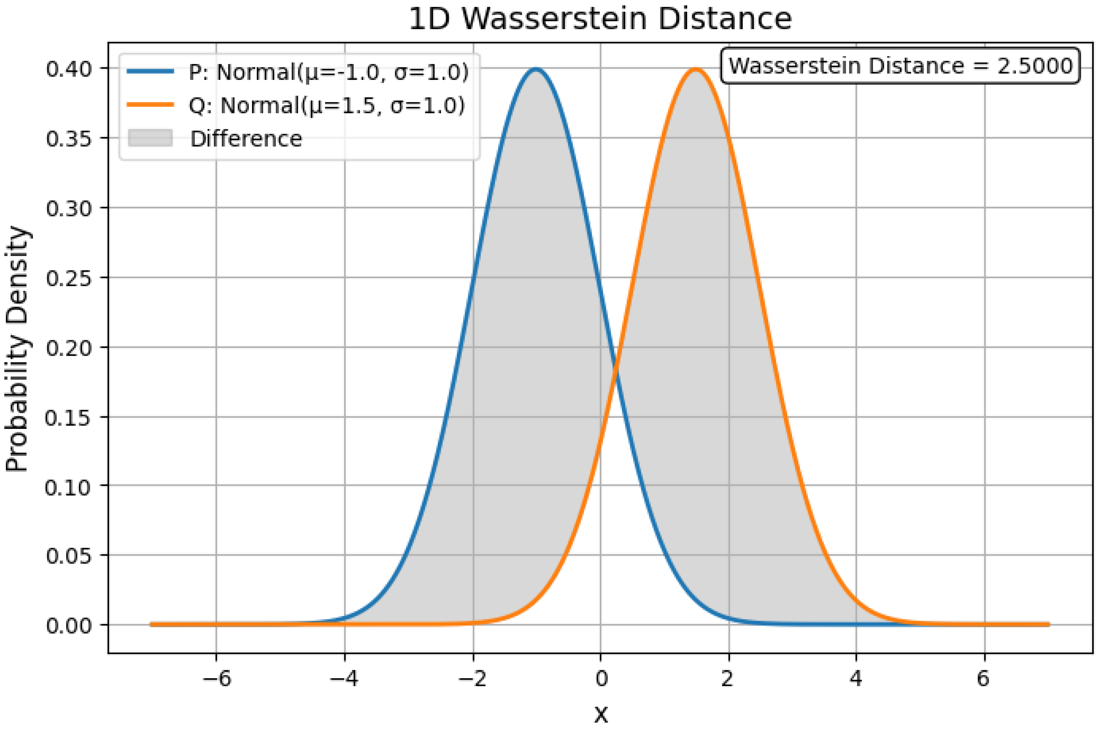
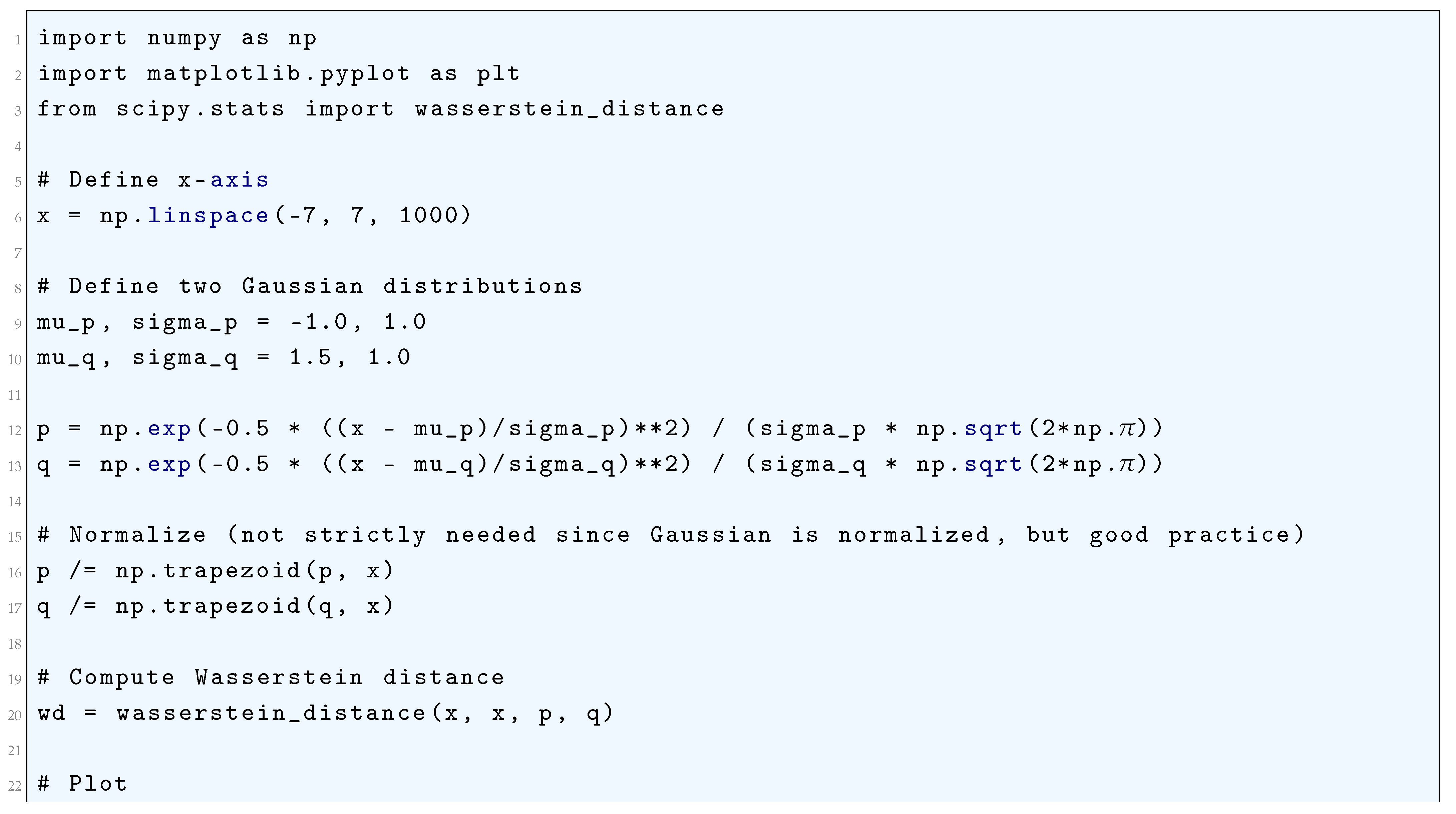
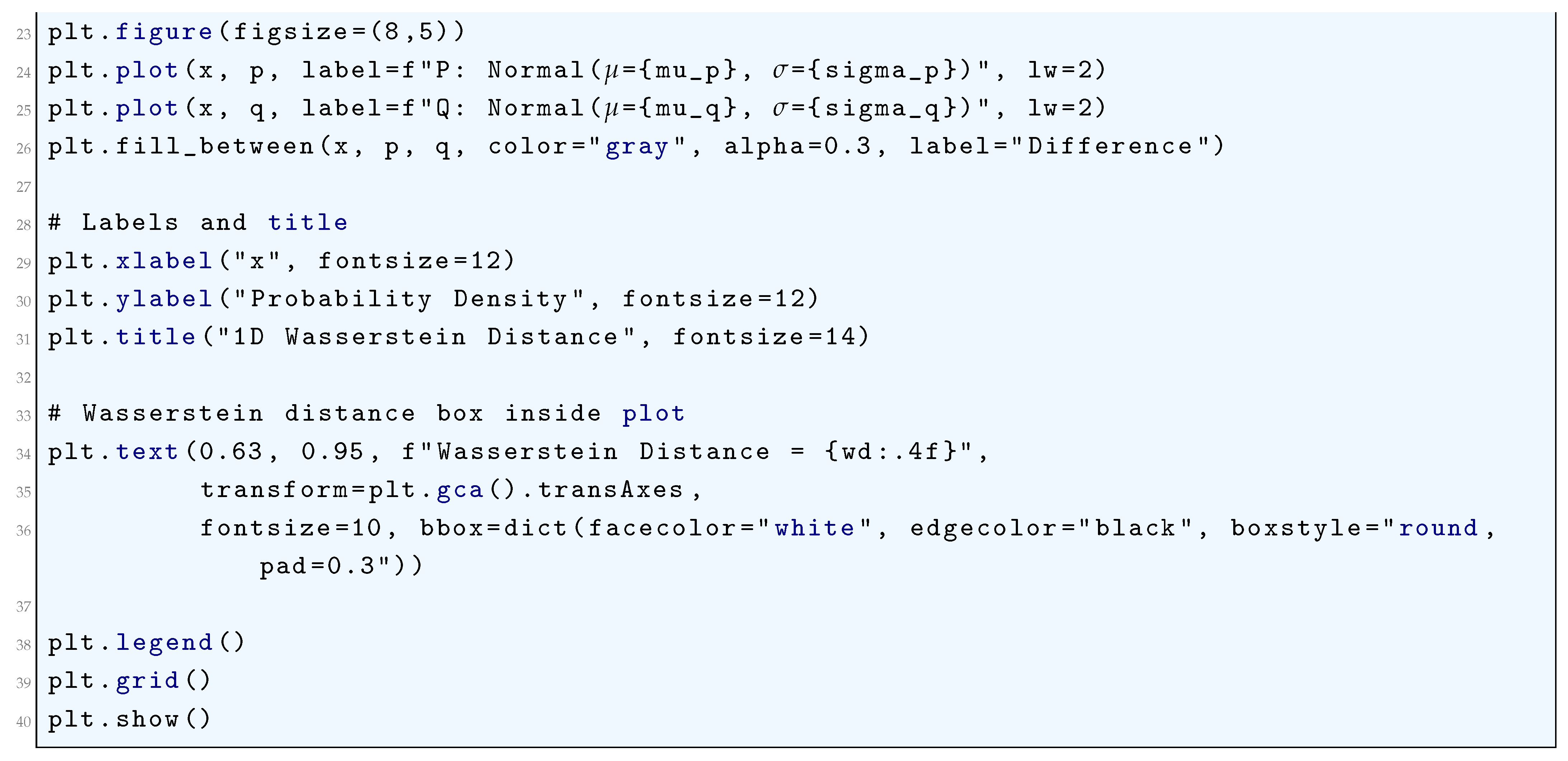
10.5.3.11 Python Code to Generate Figure 78 Illustrating Multidimensional Wasserstein Distance of Two Distributions Having Parameters, Distribution A: , Distribution B:
The Python code below produces the Figure 78 illustrating Multidimensional Wasserstein Distance of two distributions having parameters, Distribution A: , Distribution B: .
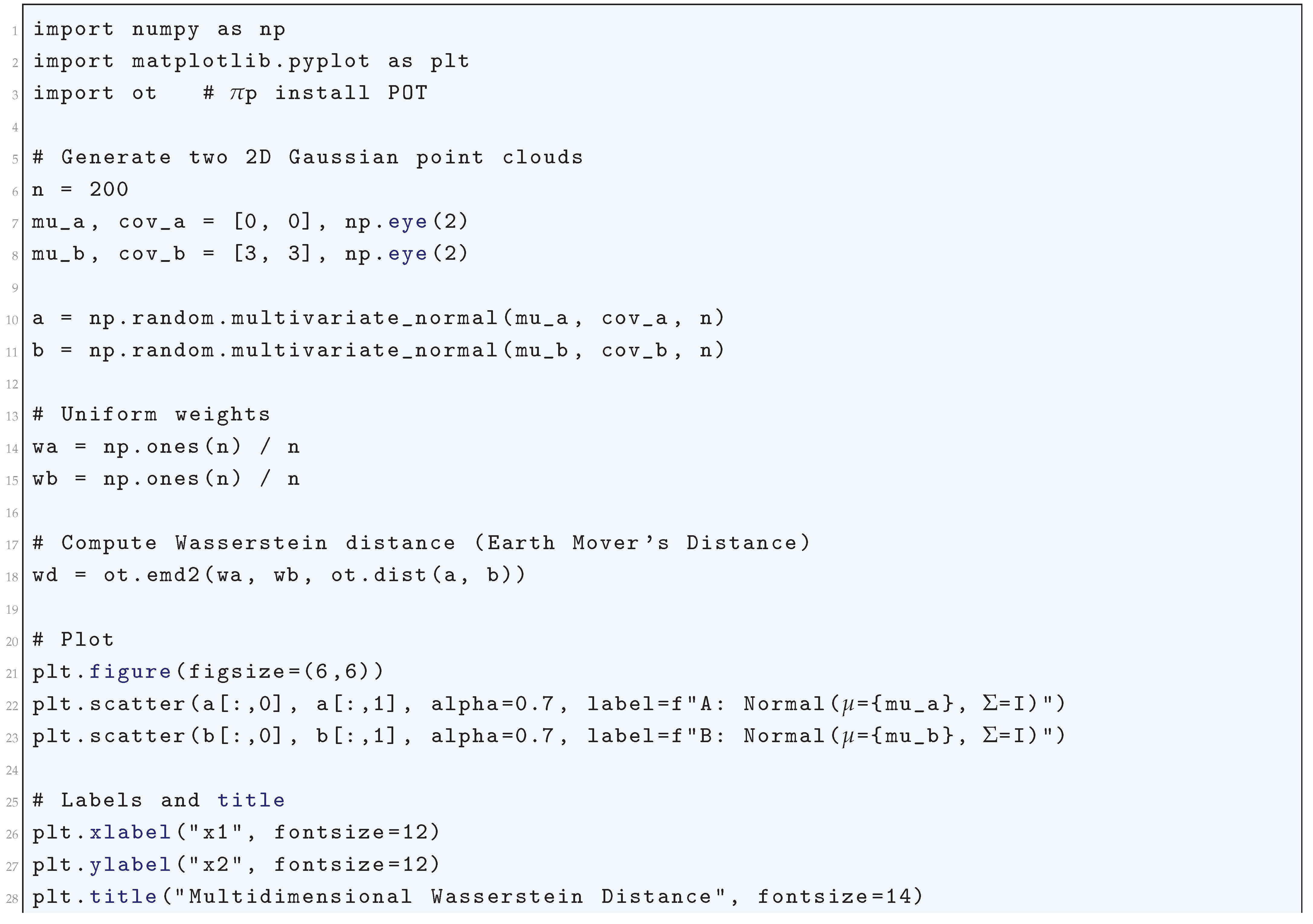
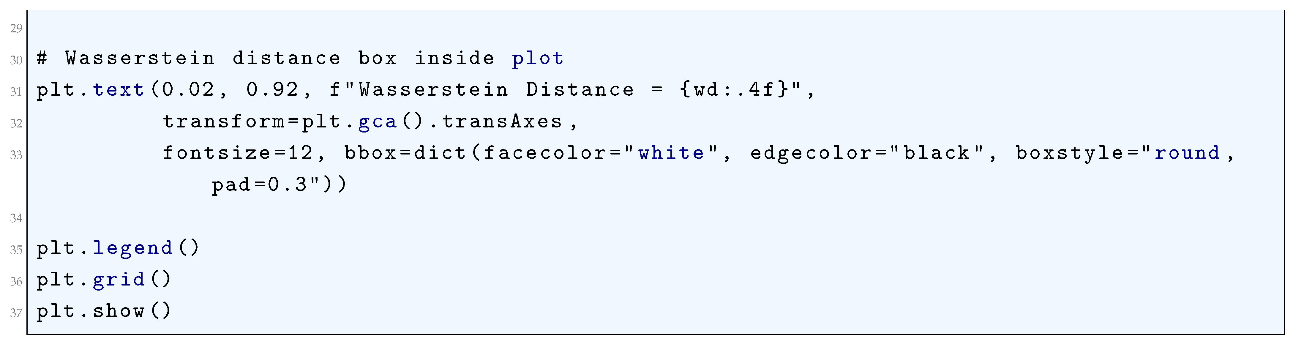
Figure 78.
Multidimensional Wasserstein Distance of two distributions having parameters, Distribution A: , Distribution B:
Figure 78.
Multidimensional Wasserstein Distance of two distributions having parameters, Distribution A: , Distribution B:
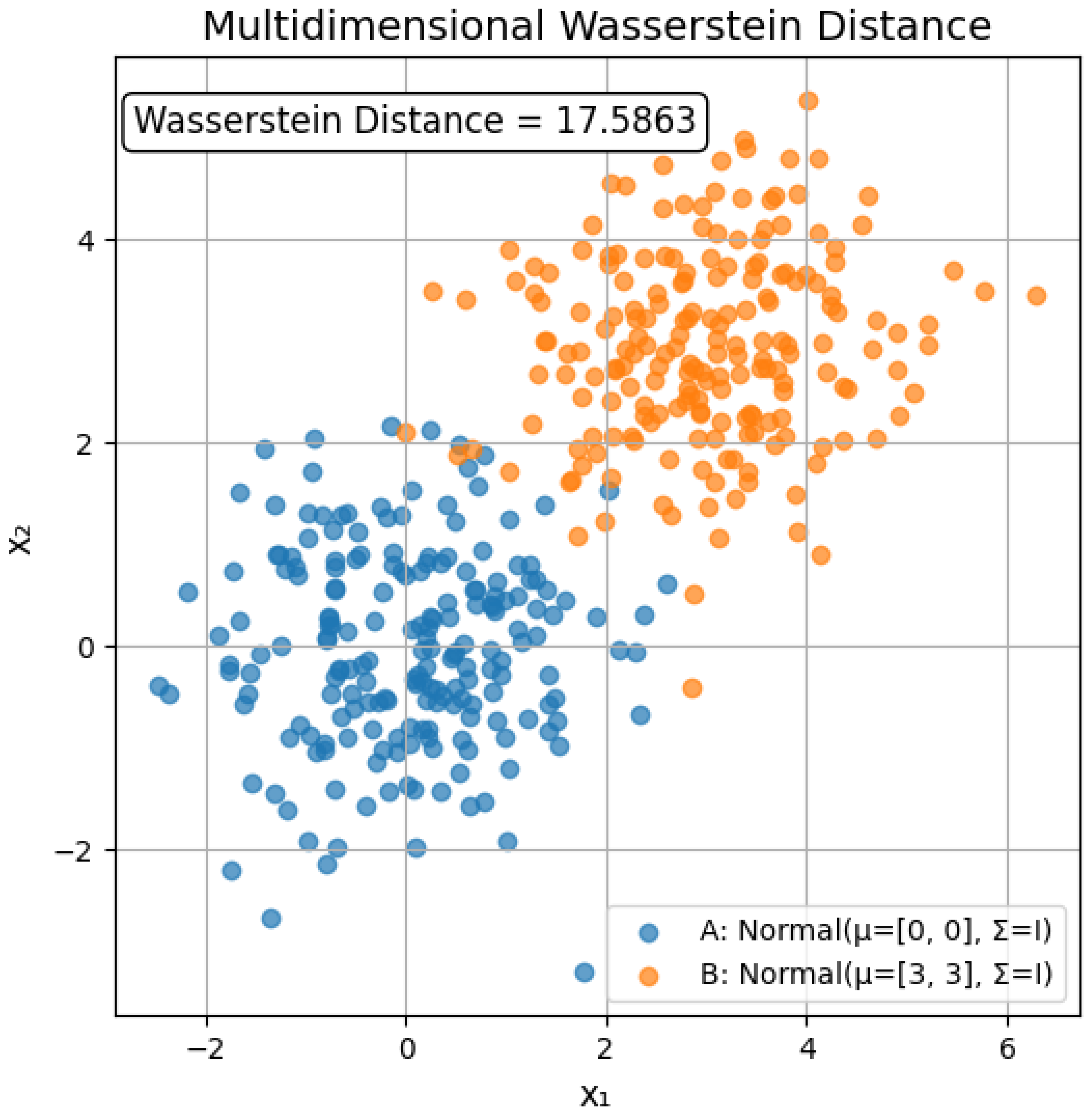
10.5.3.12 Python Code to Generate Figure 79 Comparing Equal CDF, WGAN Critic, GAN Discriminator
The Python code below produces the Figure 79 comparing Equal CDF, WGAN Critic, GAN Discriminator.
Figure 79.
Comparison: Equal CDF, WGAN Critic, GAN Discriminator
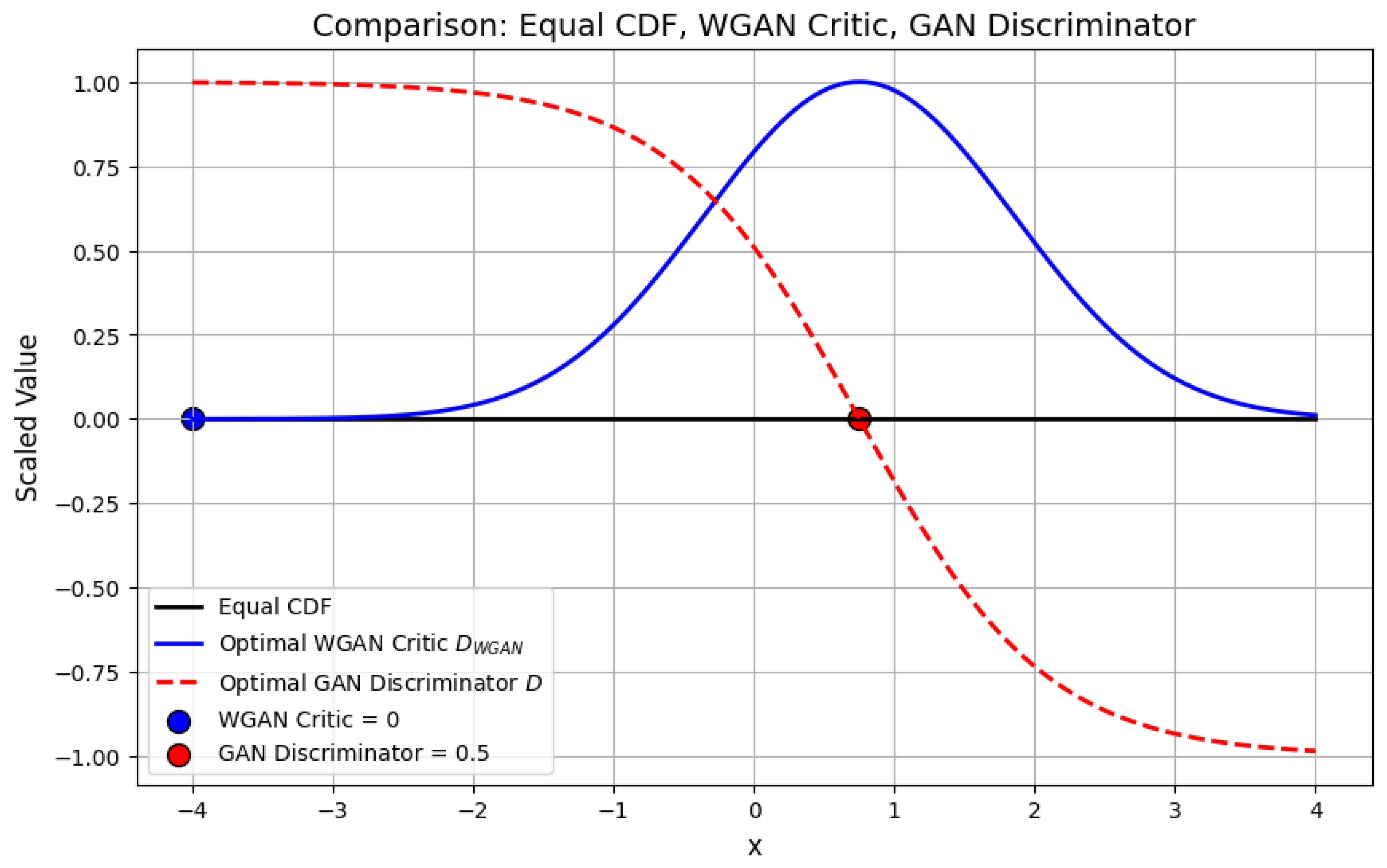
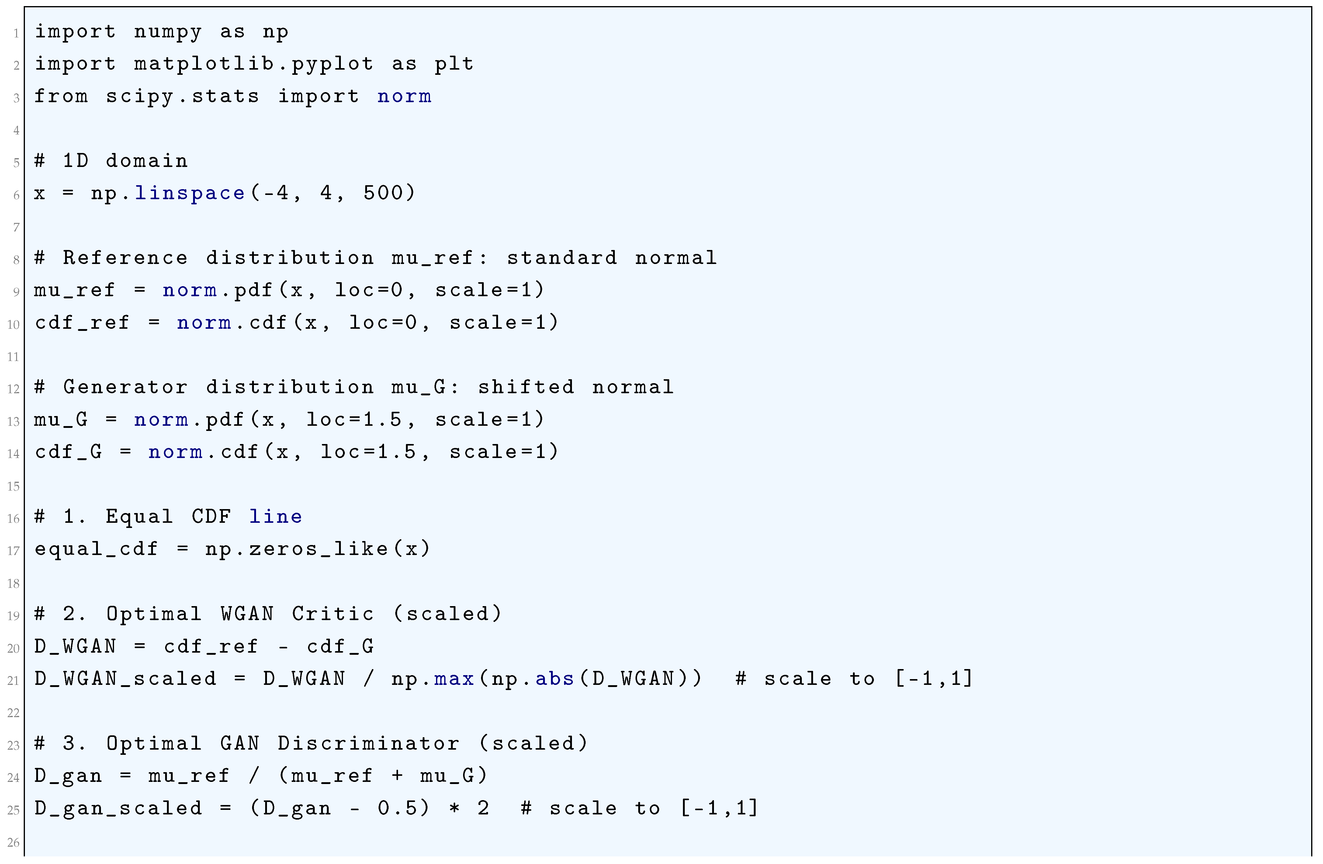
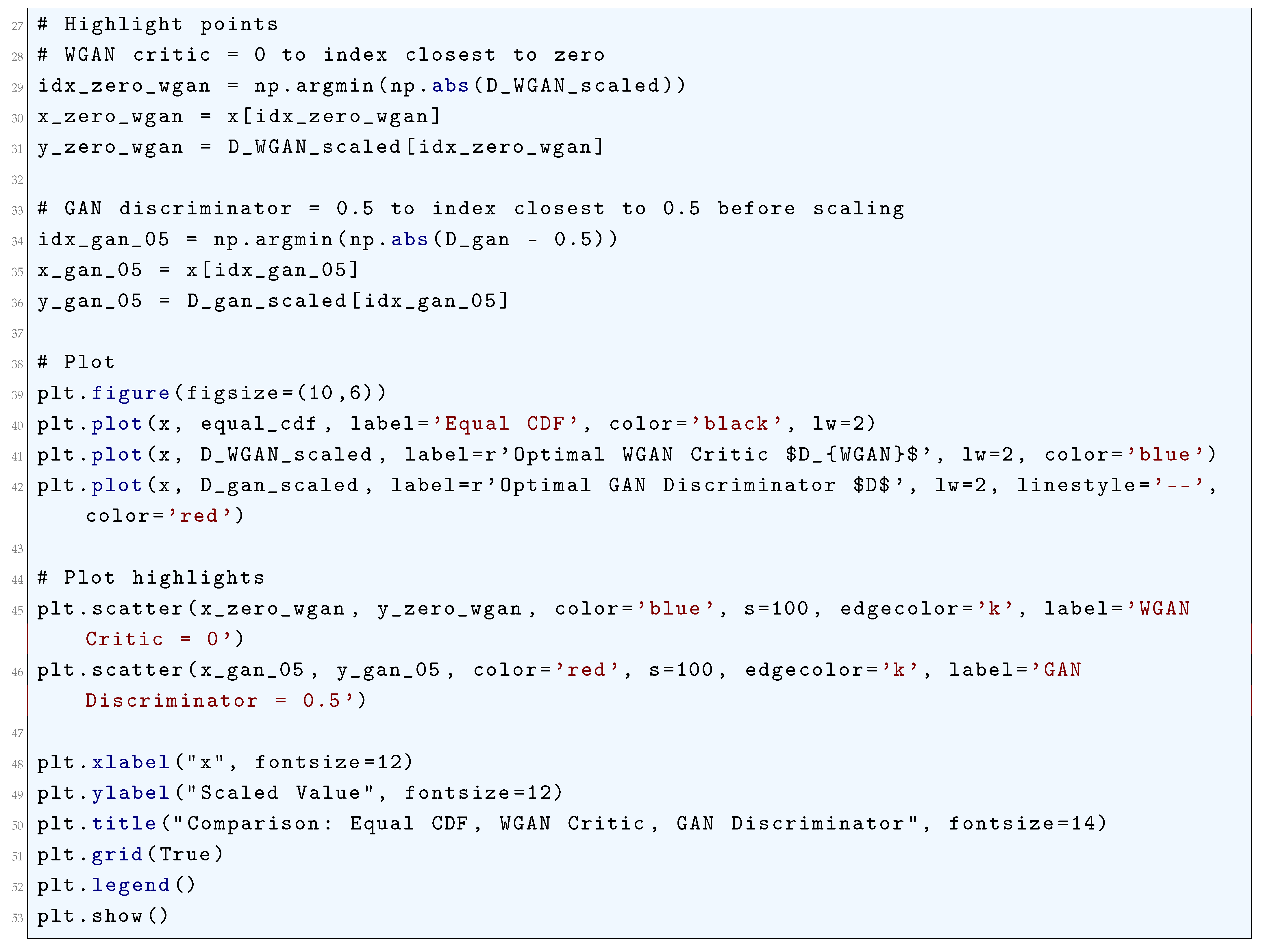
10.5.3.13 Python Code to Generate Figure 80 Illustrating Least Squares GAN (LSGAN) Loss Functions
The Python code below produces the Figure 80 illustrating Least Squares GAN (LSGAN) Loss Functions.
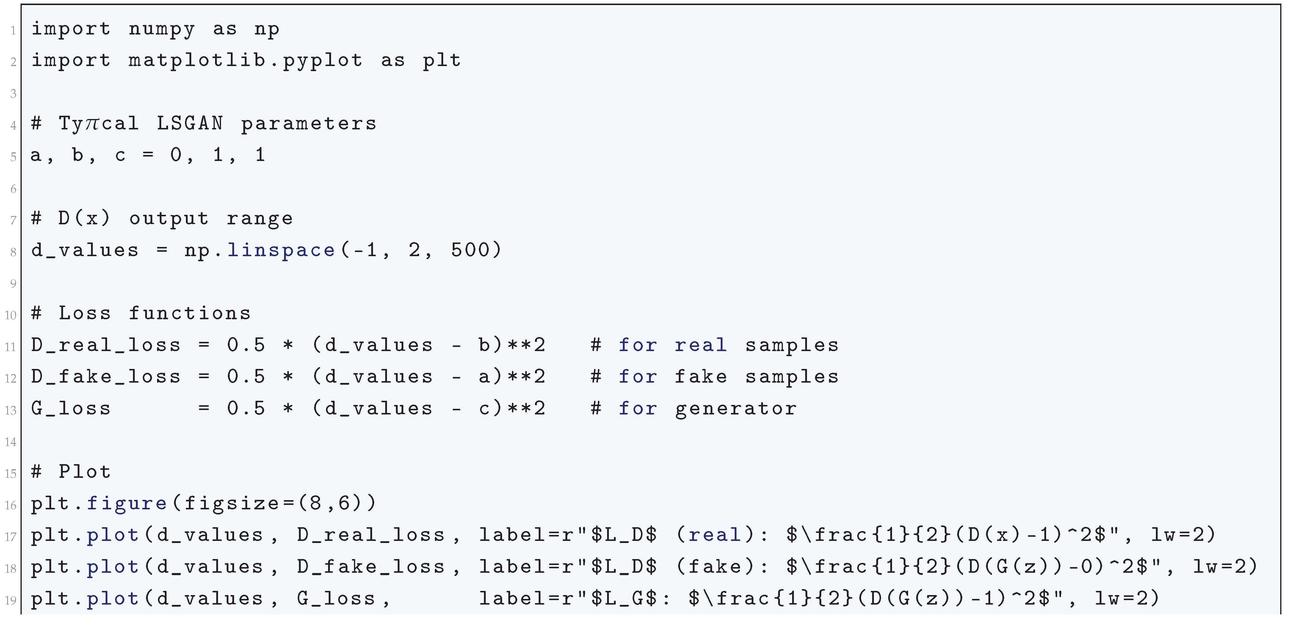
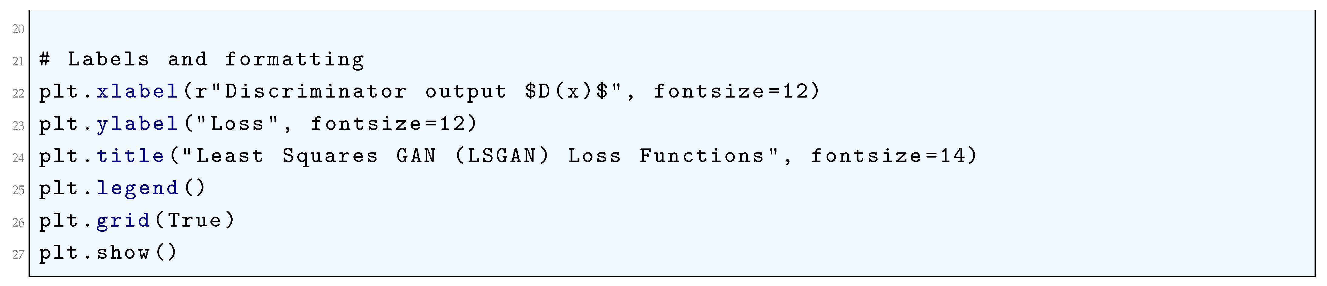
Figure 80.
Least Squares GAN (LSGAN) Loss Functions
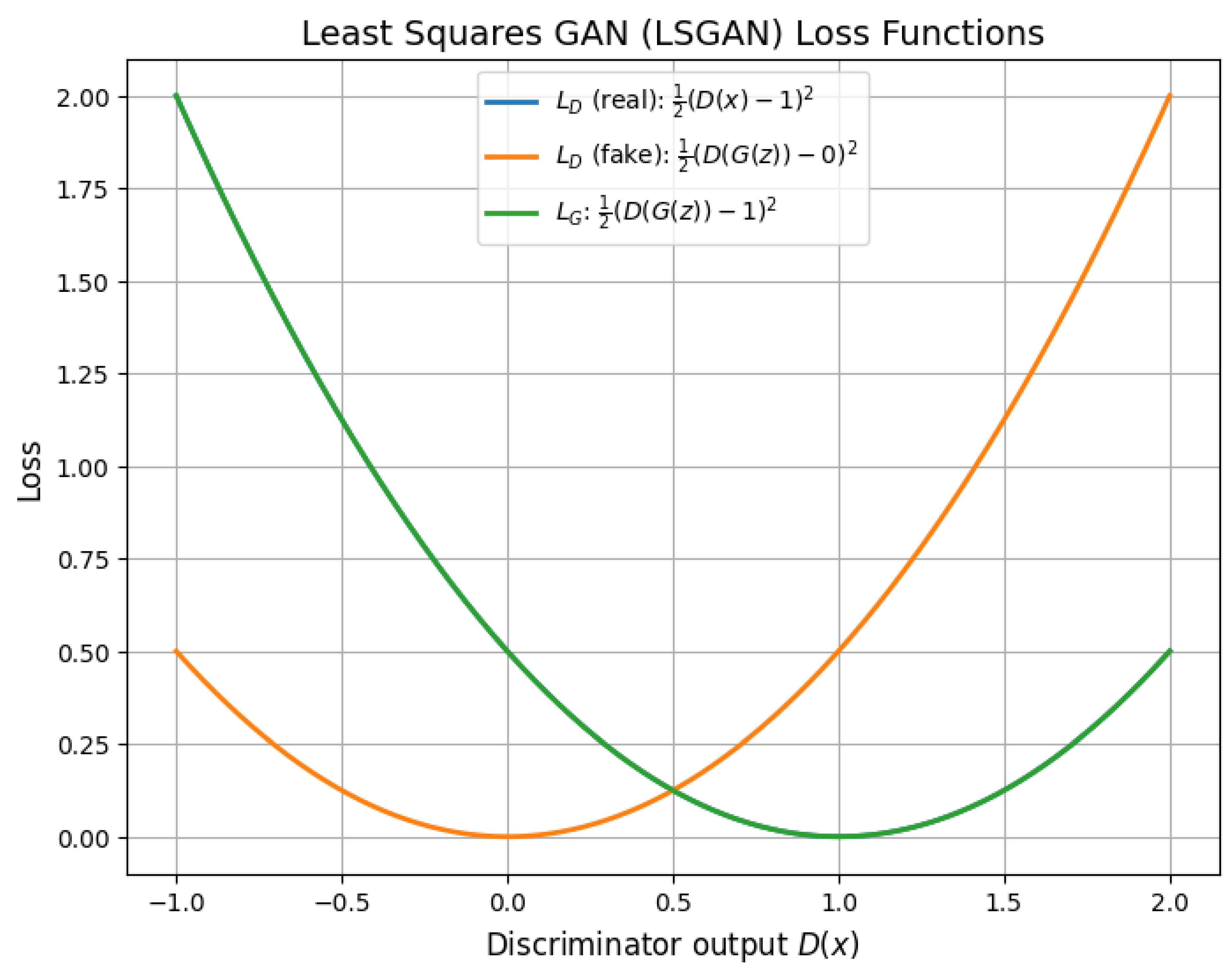
10.5.3.14 Python Code to Generate Figure 81 Illustrating Standard GAN (Adversarial) Loss Functions
The Python code below produces the Figure 81 illustrating Standard GAN (Adversarial) Loss Functions.
Figure 81.
Standard GAN (Adversarial) Loss Functions
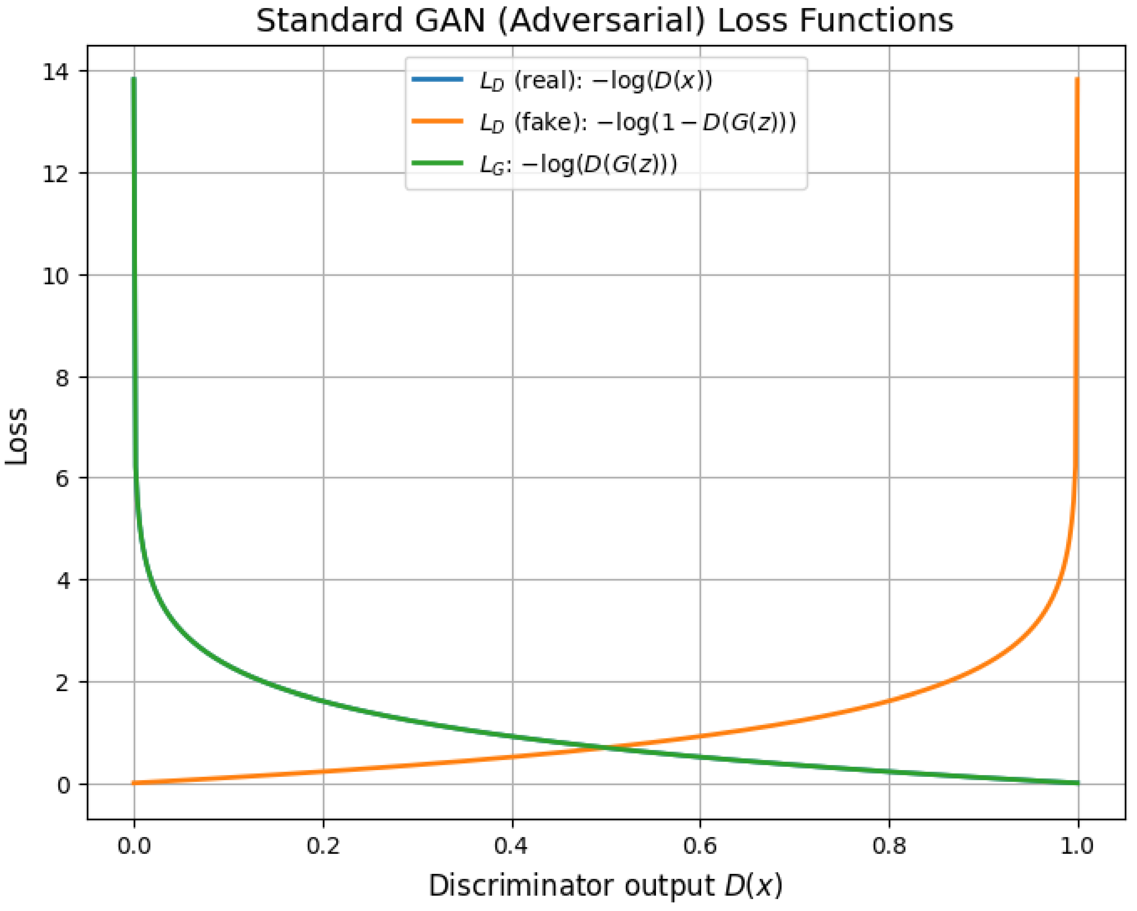
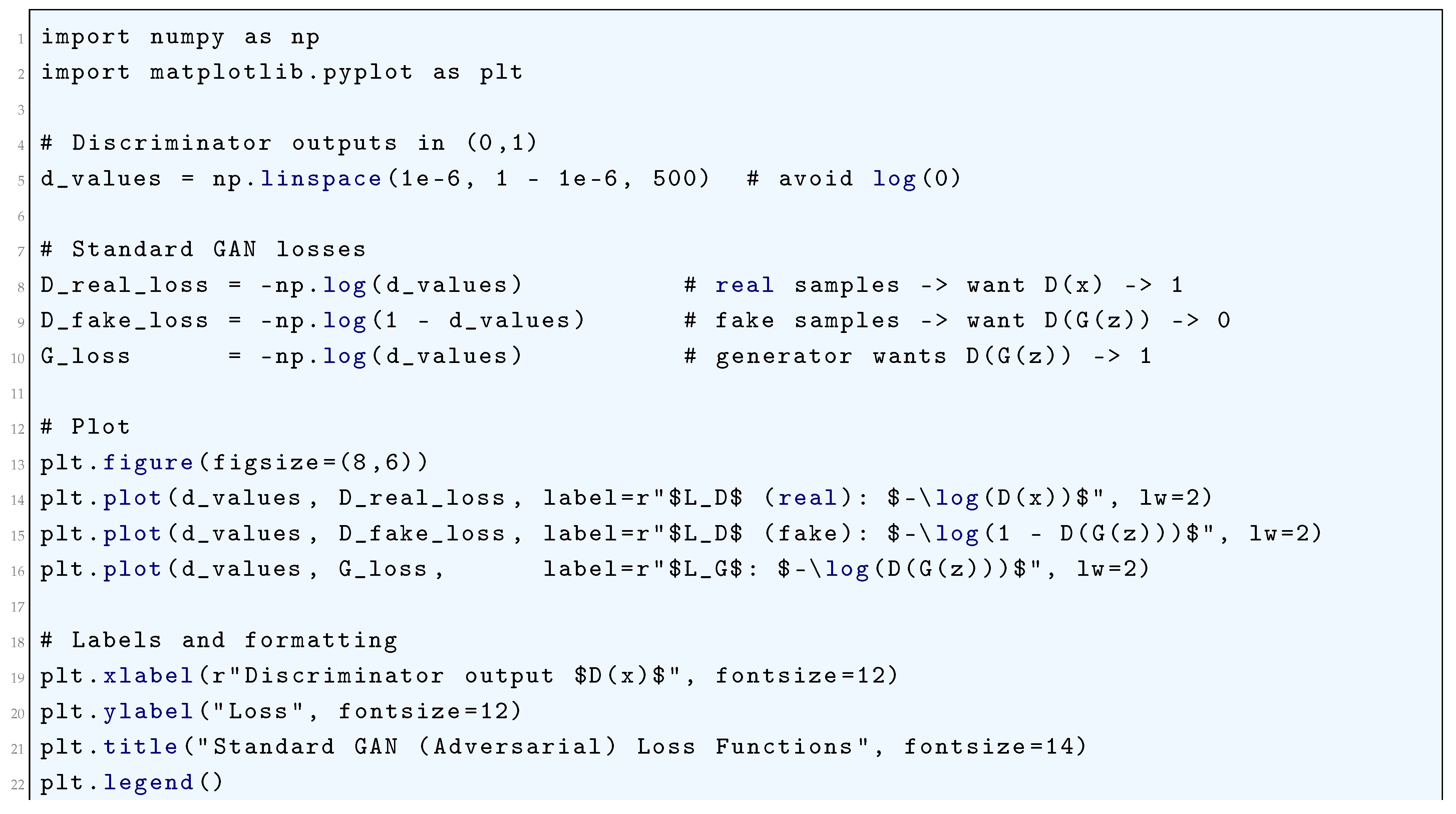

10.5.3.15 Python Code to Generate Figure 82 Illustrating Contrastive Loss Functions
The Python code below produces the Figure 82 illustrating Contrastive Loss Functions.
Figure 82.
Contrastive Loss Functions
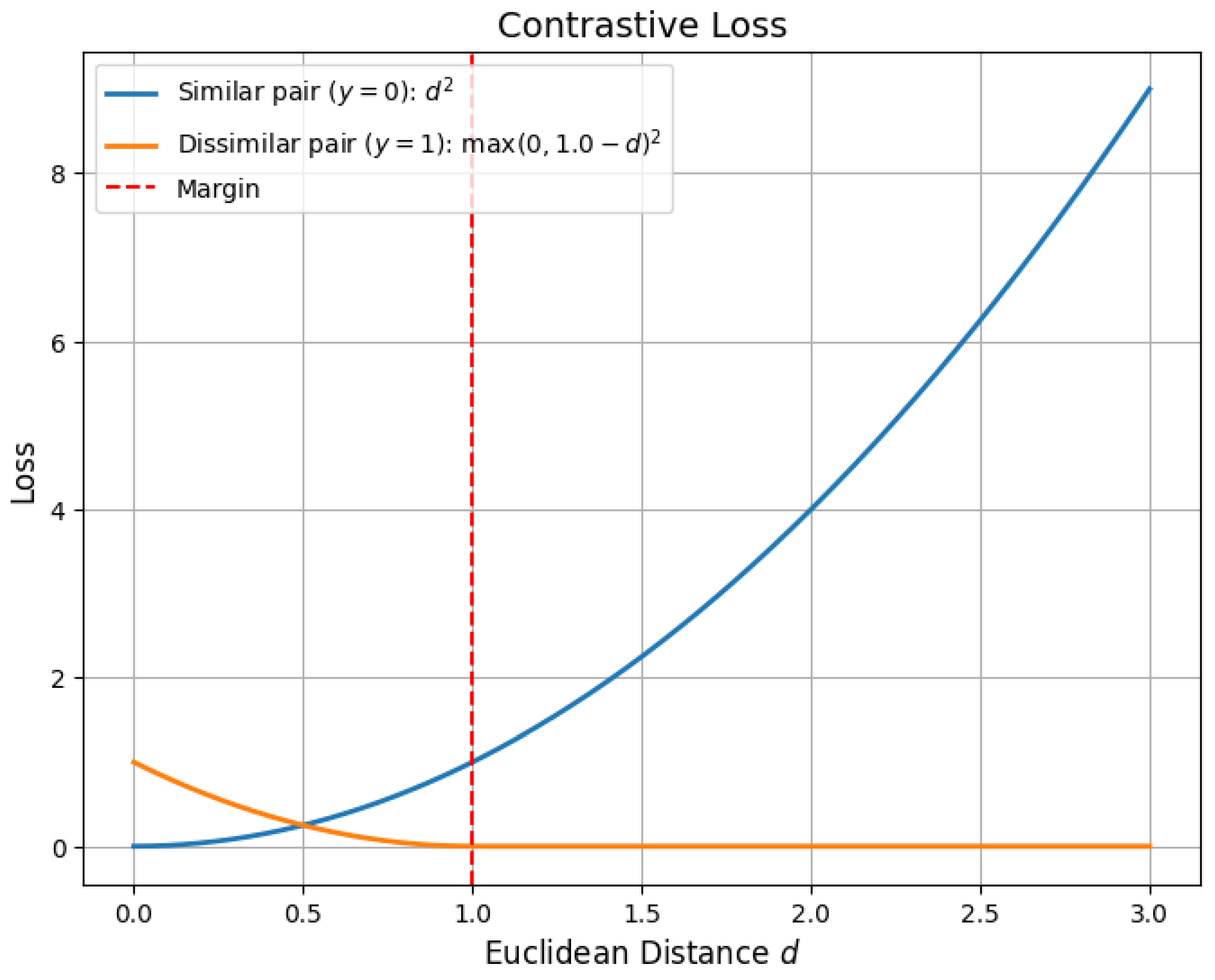
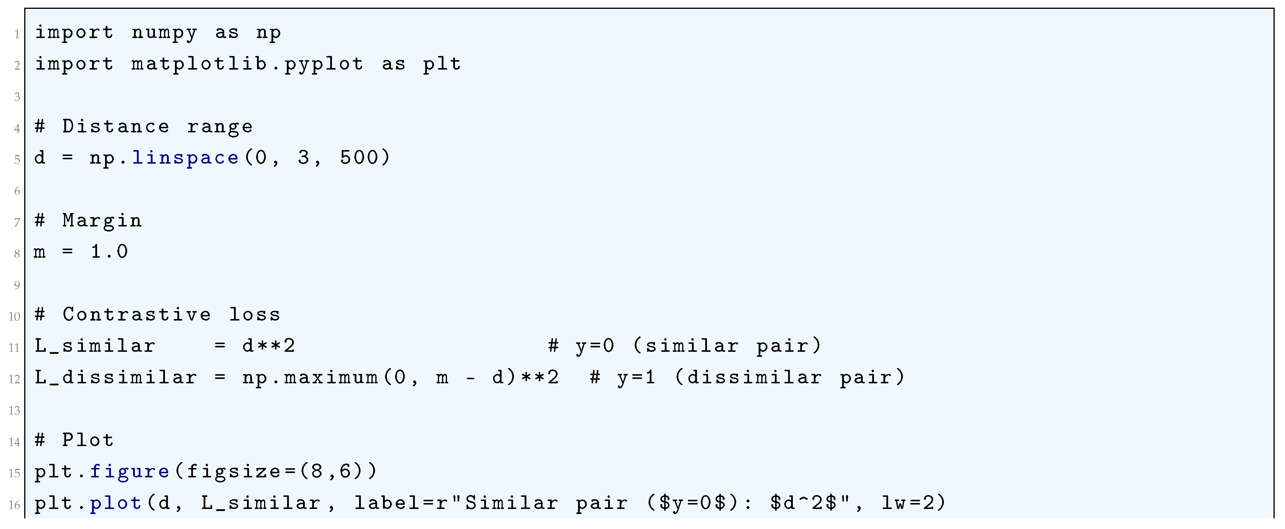
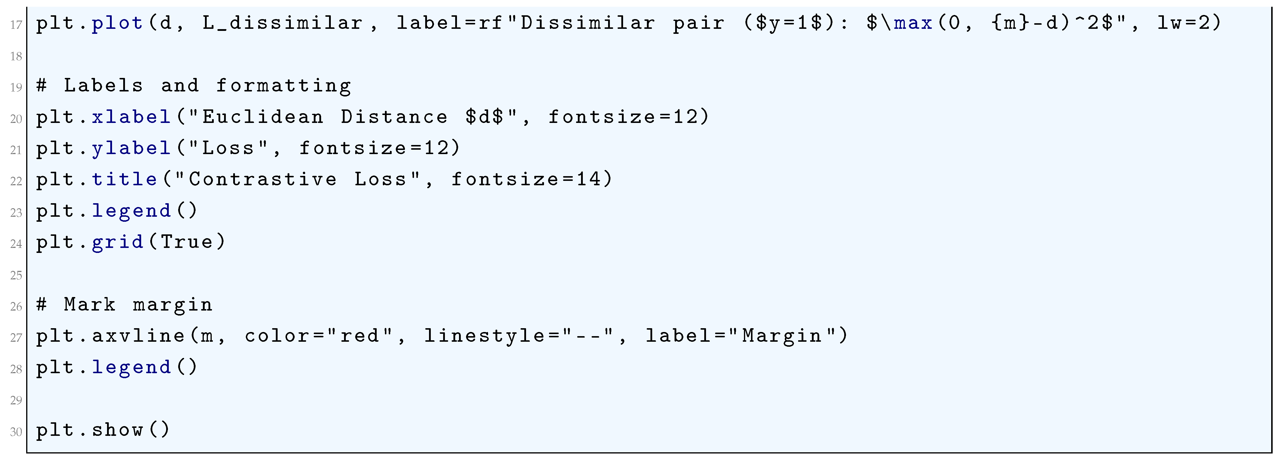
10.5.3.16 Python Code to Generate Figure 83 Illustrating Contrastive Loss Landscapes
The Python code below produces the Figure 83 illustrating Contrastive Loss Landscapes.
Figure 83.
Contrastive Loss Landscapes
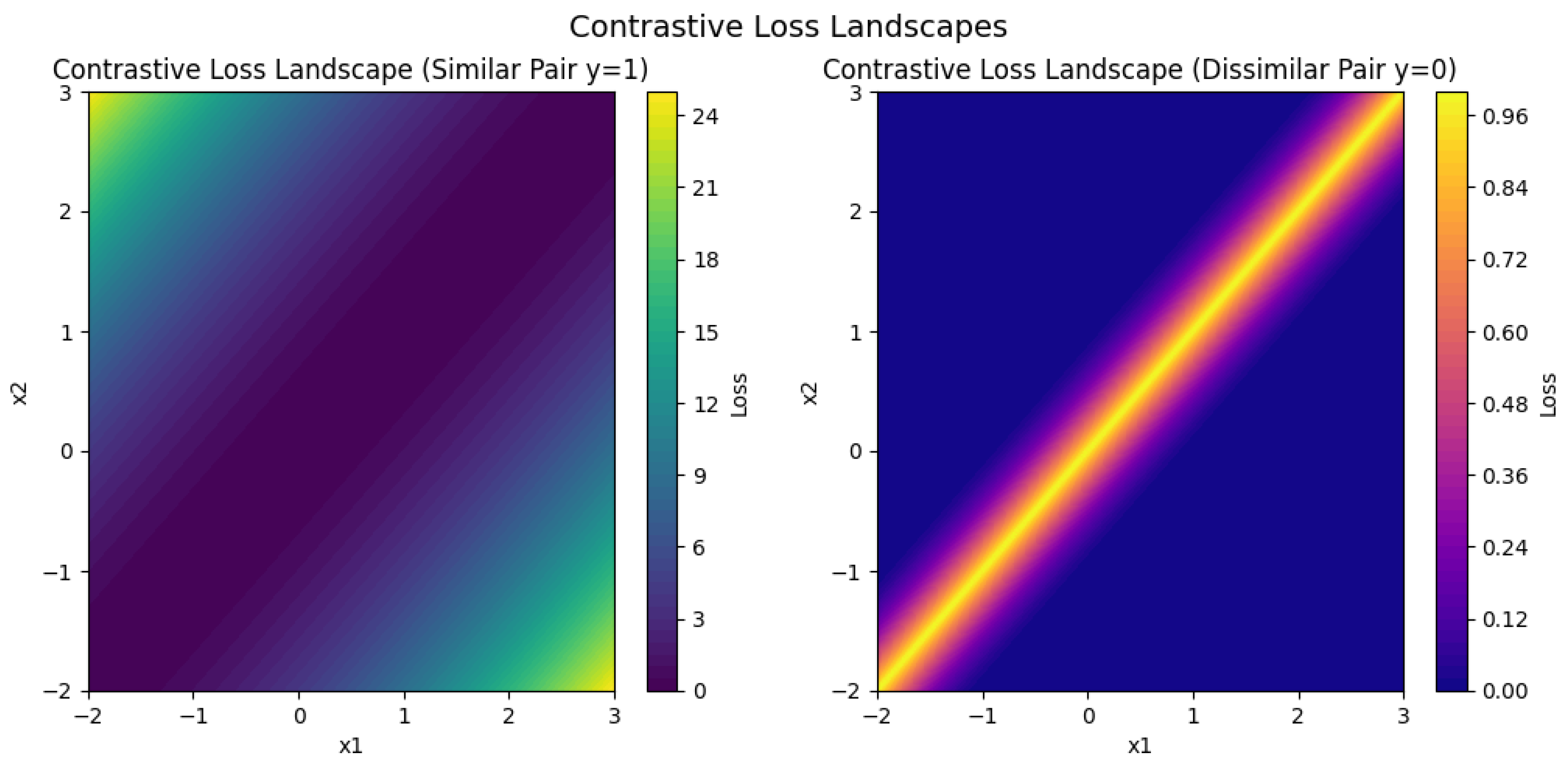
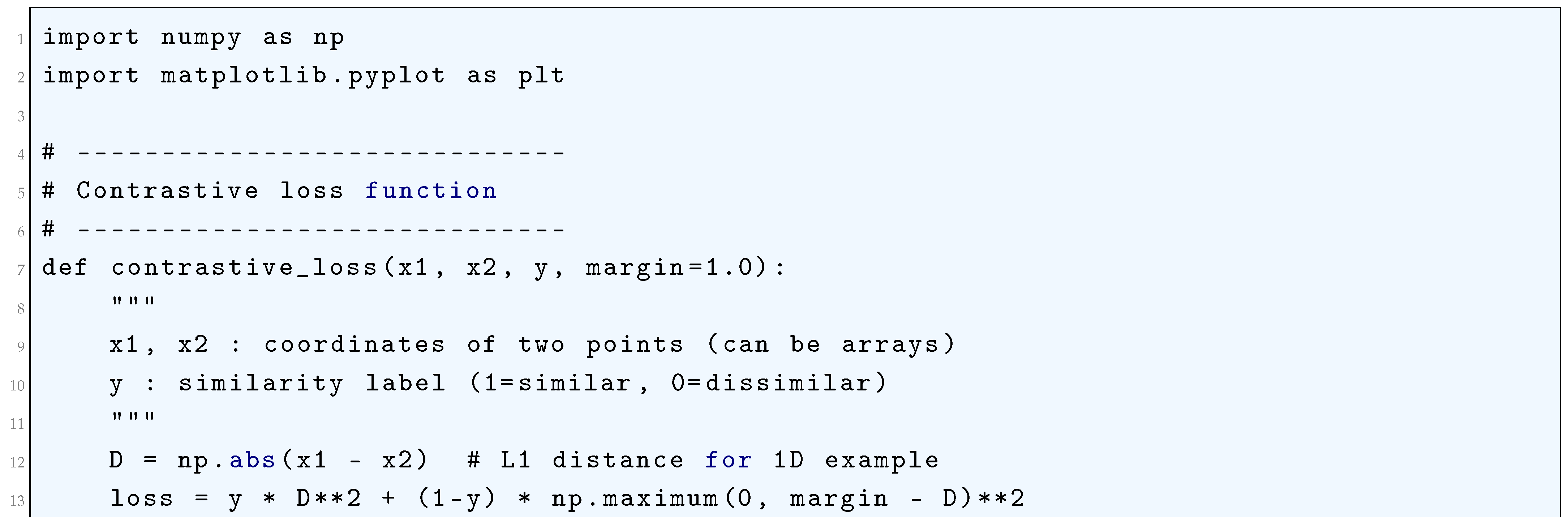
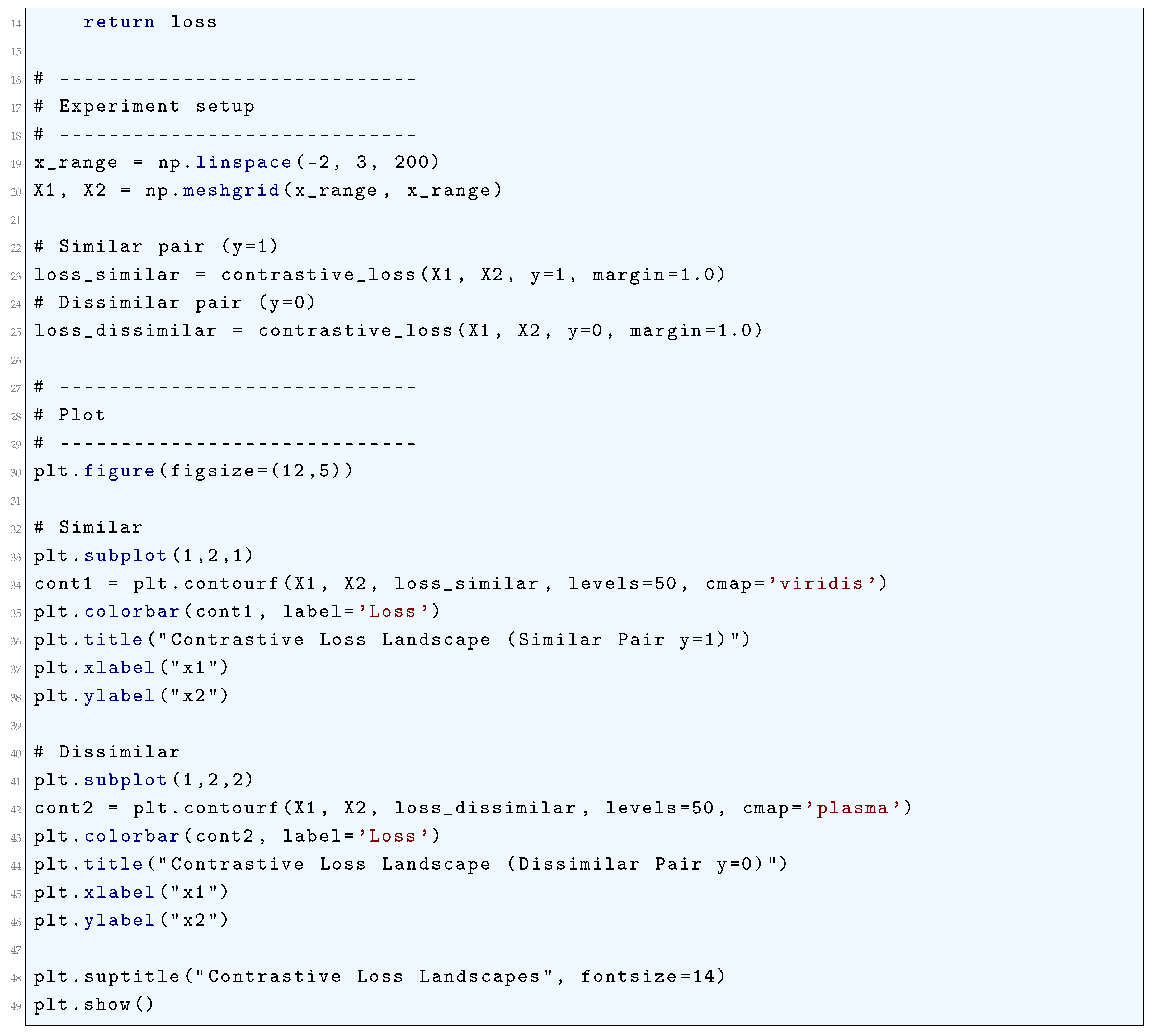
10.5.3.17 Python Code to Generate Figure 84 Illustrating 3D Contrastive Loss Landscapes
The Python code below produces the Figure 84 illustrating 3D Contrastive Loss Landscapes.
Figure 84.
3D Contrastive Loss Landscapes
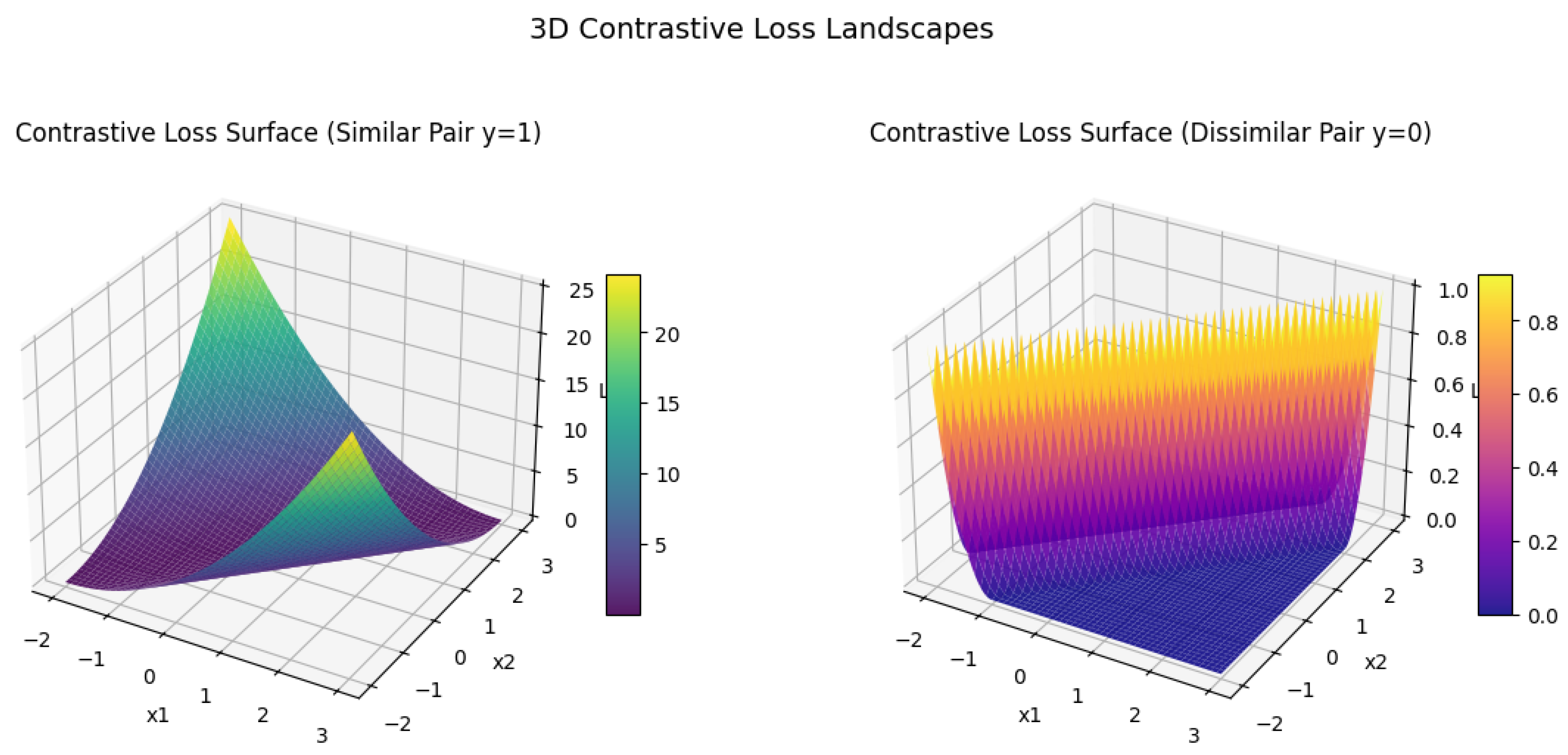
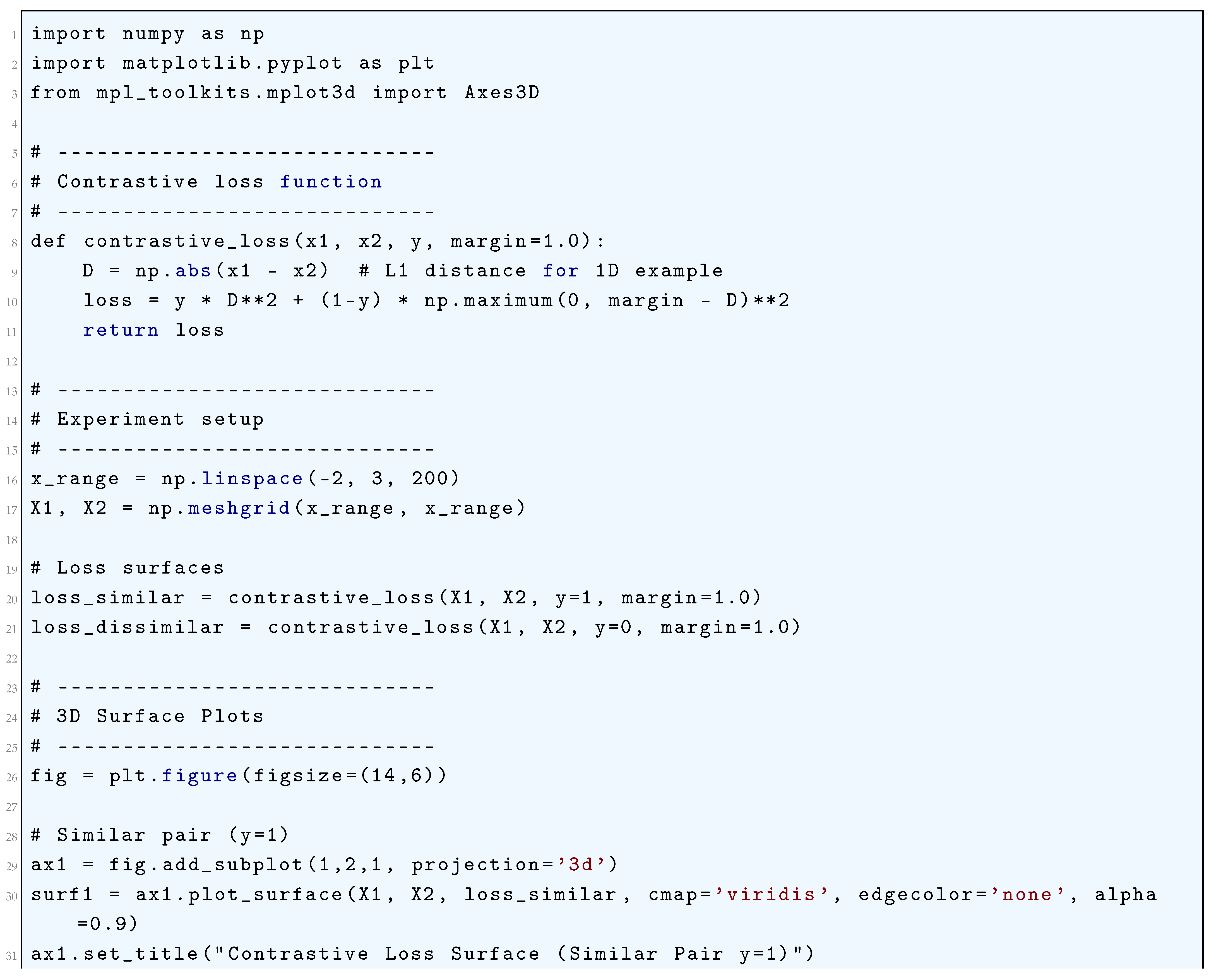
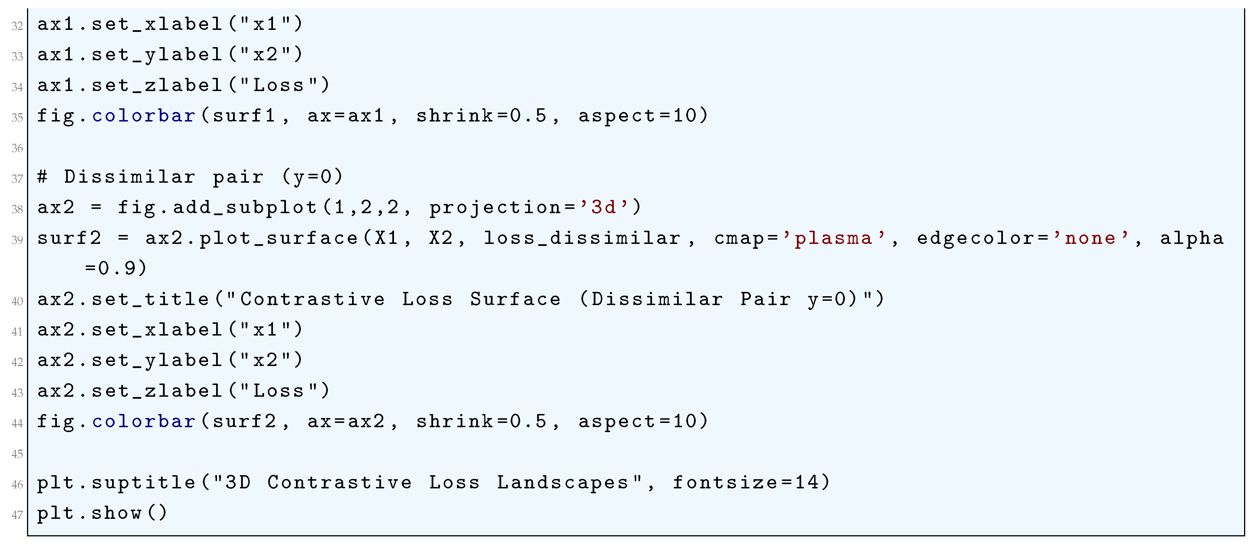
10.5.3.18 Python Code to Generate Figure 85 Illustrating Triplet Loss Function
The Python code below produces the Figure 85 illustrating Triplet Loss Function.
Figure 85.
Triplet Loss Function
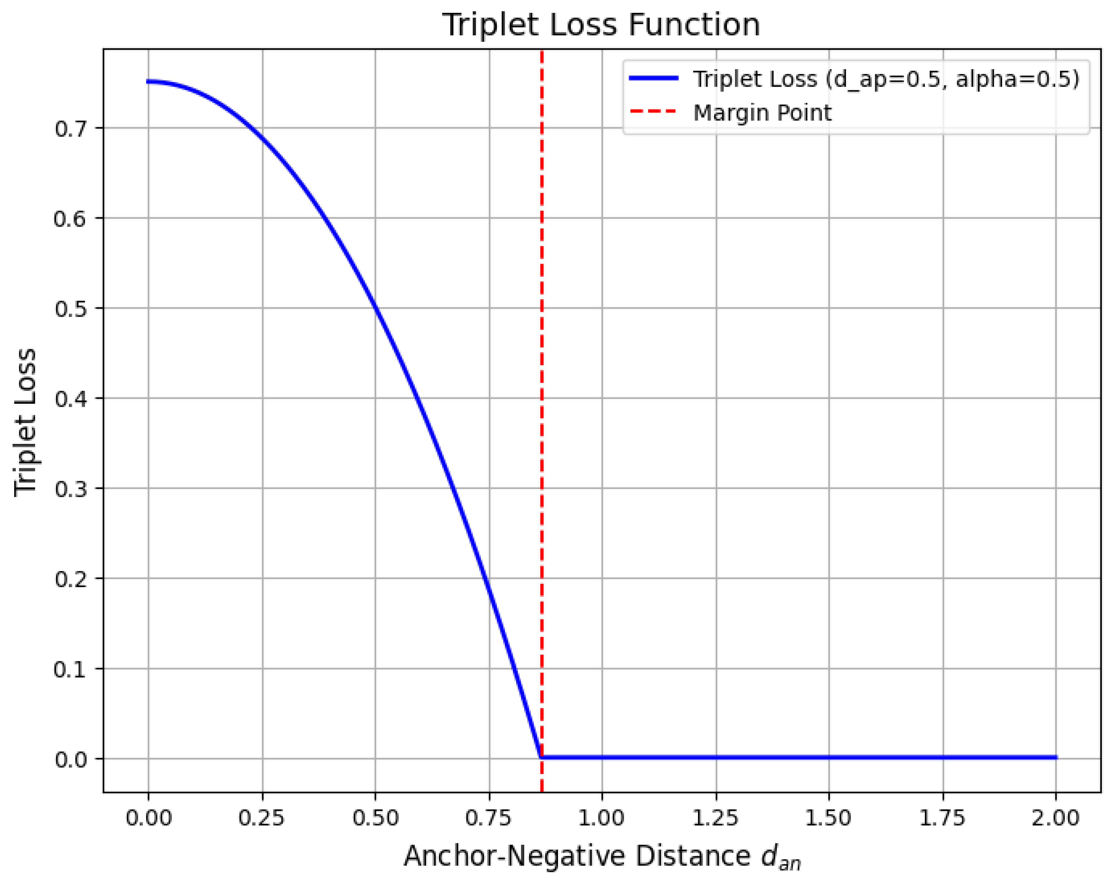
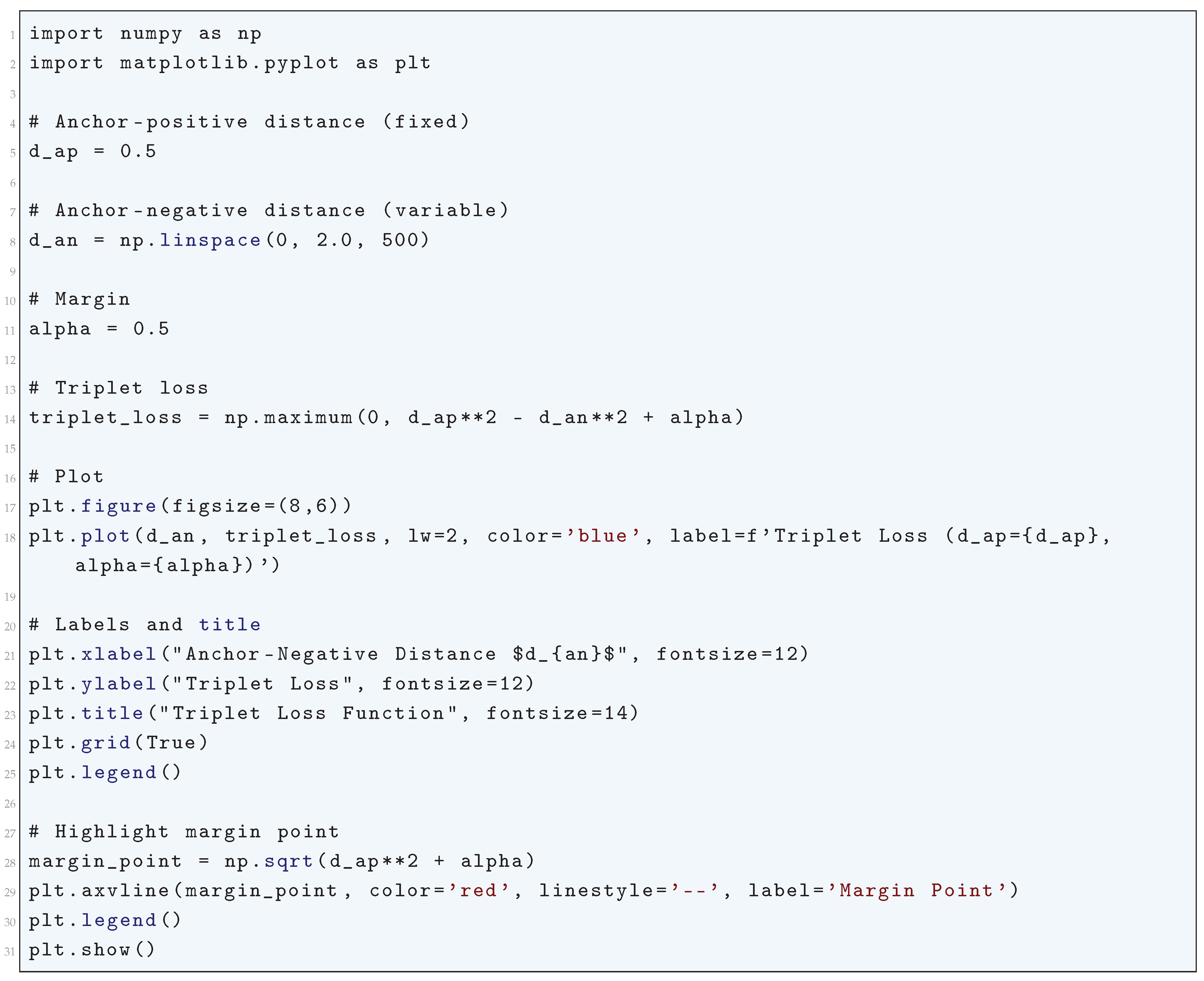
10.5.3.19 Python Code to Generate Figure 86 Illustrating Triplet Loss Landscape
The Python code below produces the Figure 86 illustrating Triplet Loss Landscape.
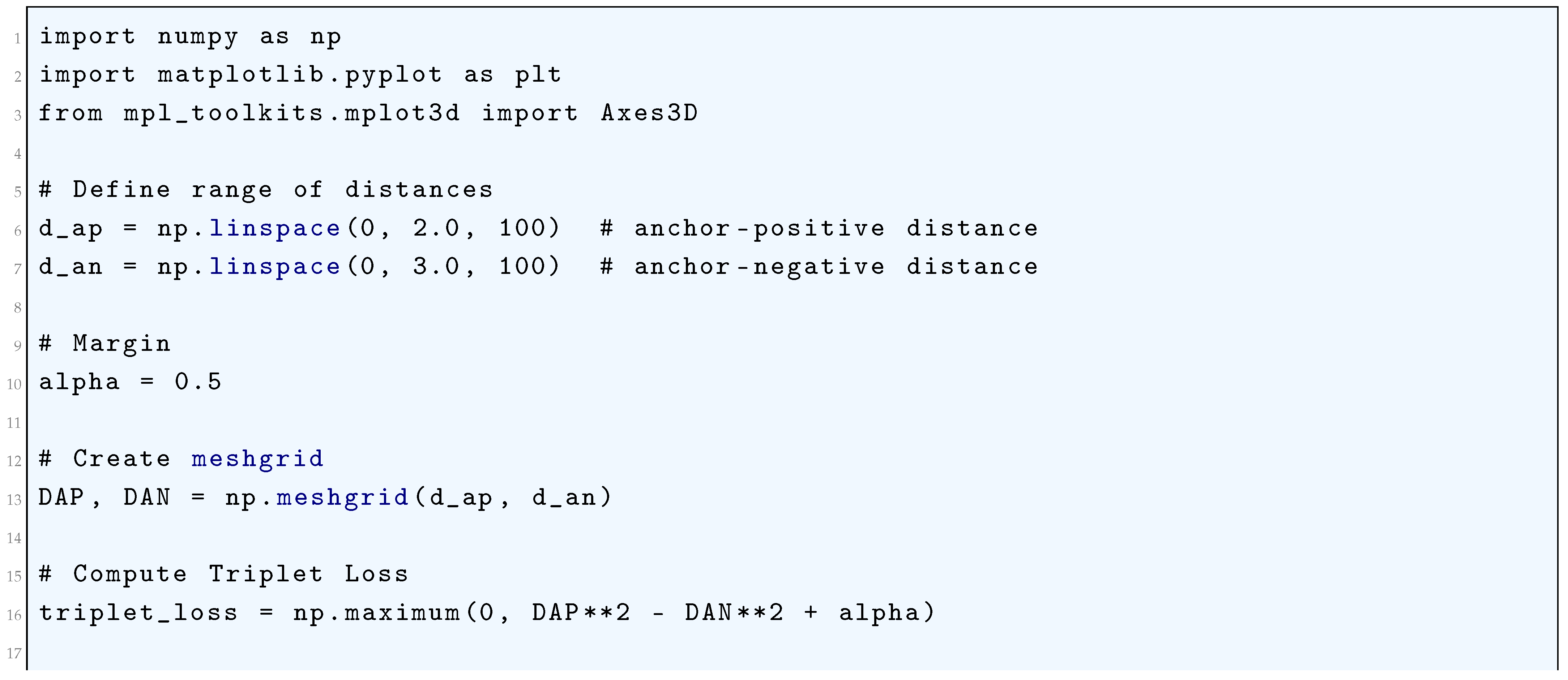
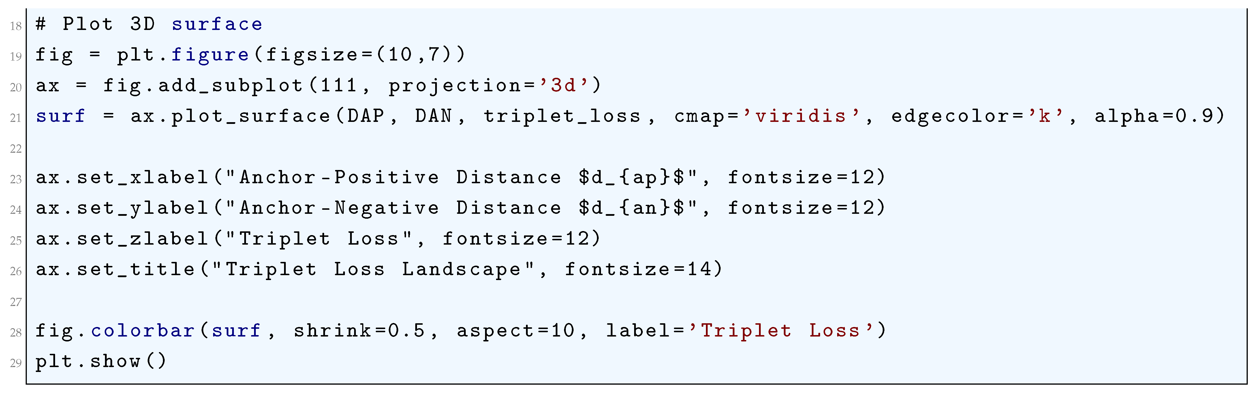
Figure 86.
Triplet Loss Landscape
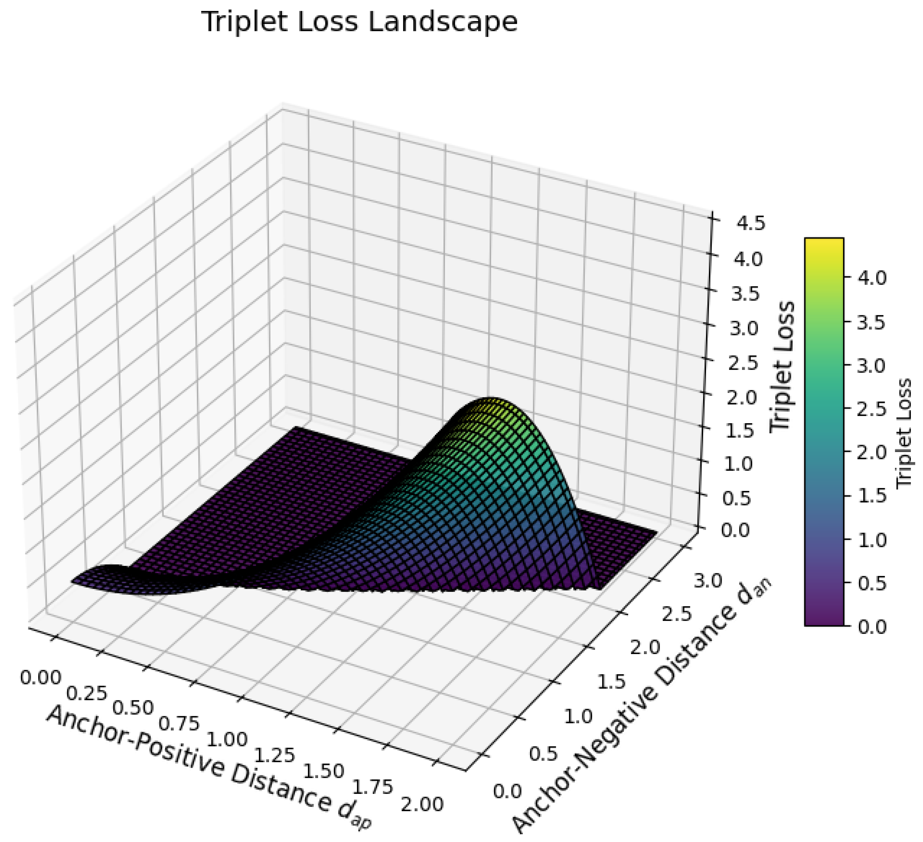
10.5.3.20 Python Code to Generate Figure 87 Illustrating Triplet Loss Contour Plot
The Python code below produces the Figure 87 illustrating Triplet Loss Contour Plot.
Figure 87.
Triplet Loss Contour Plot
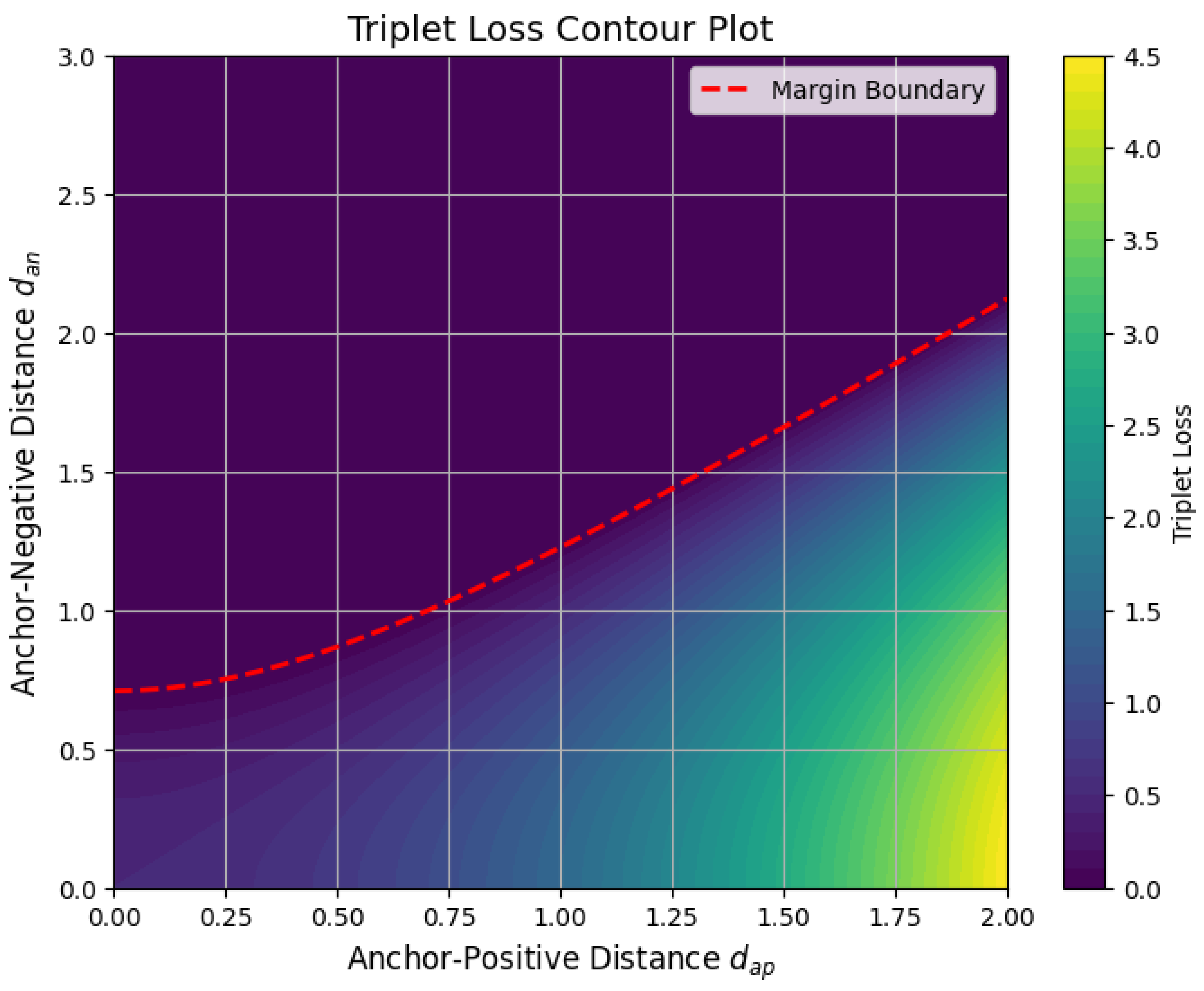
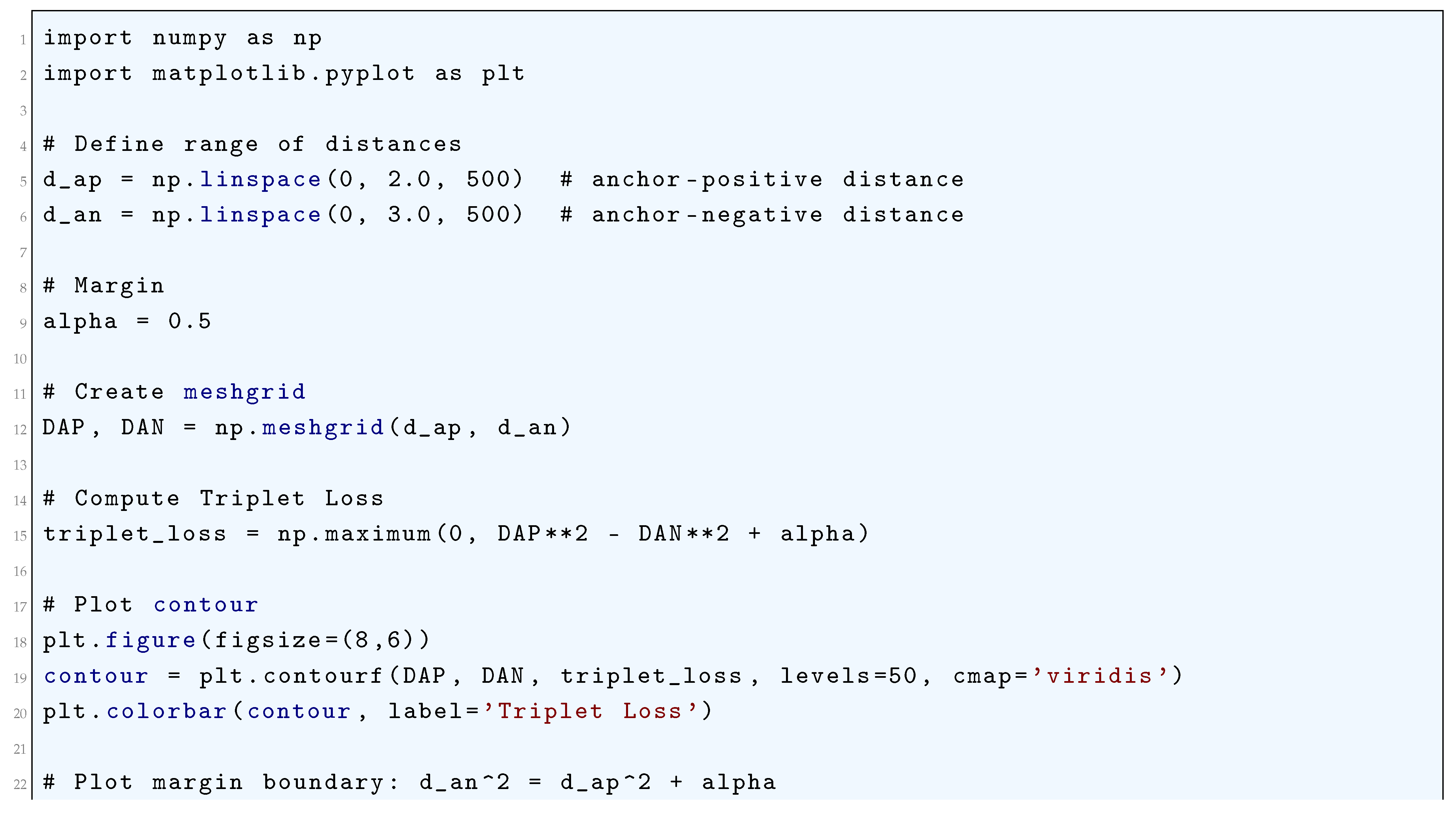
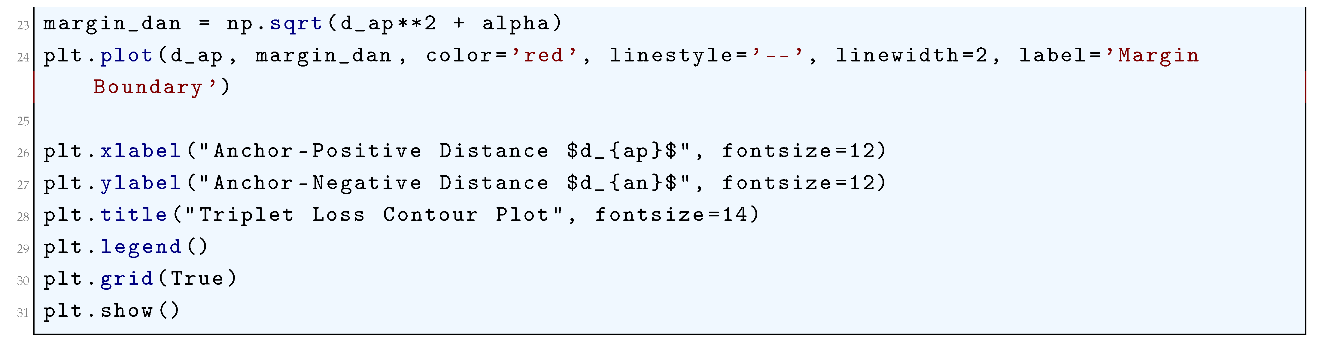
10.5.3.21 Python Code to Generate Figure 88 Illustrating Center Loss Function
The Python code below produces the Figure 88 illustrating Center Loss Function.
Figure 88.
Center Loss Function
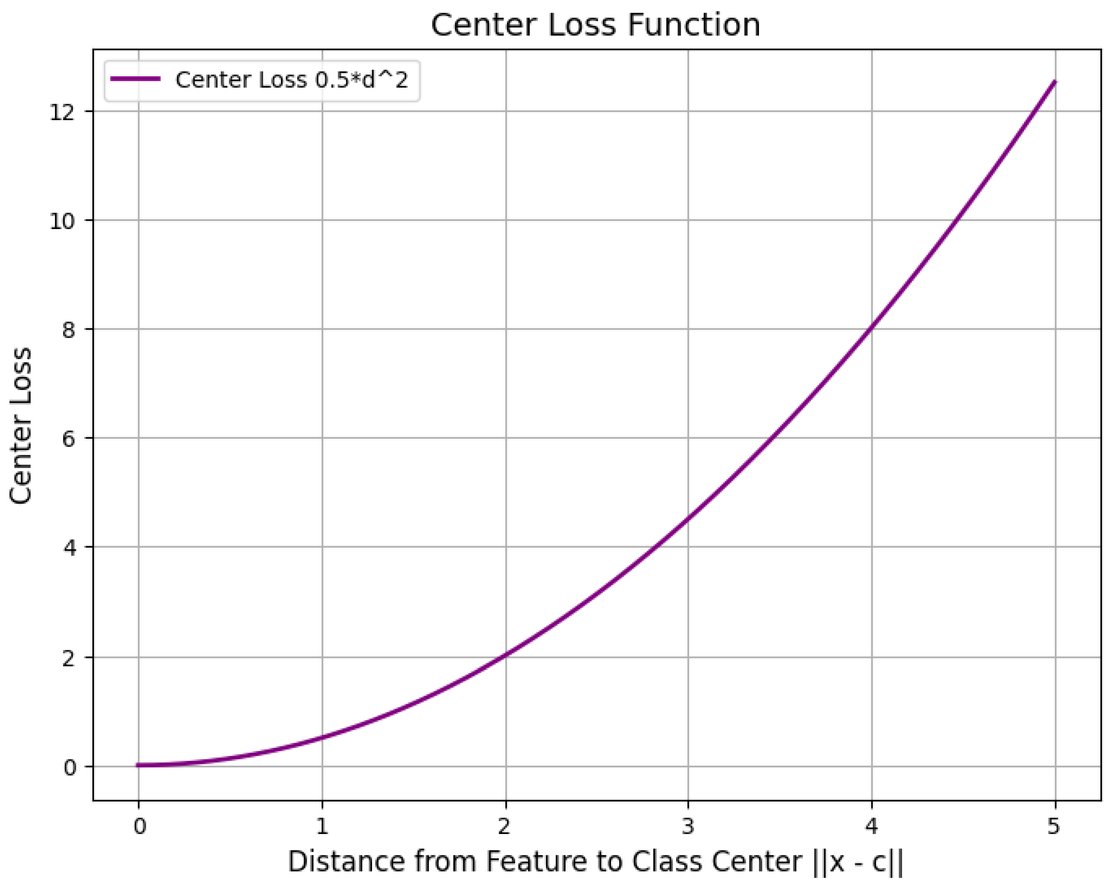
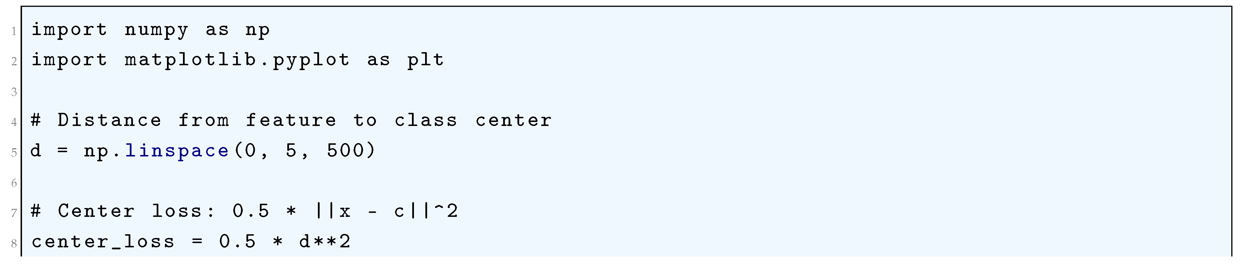
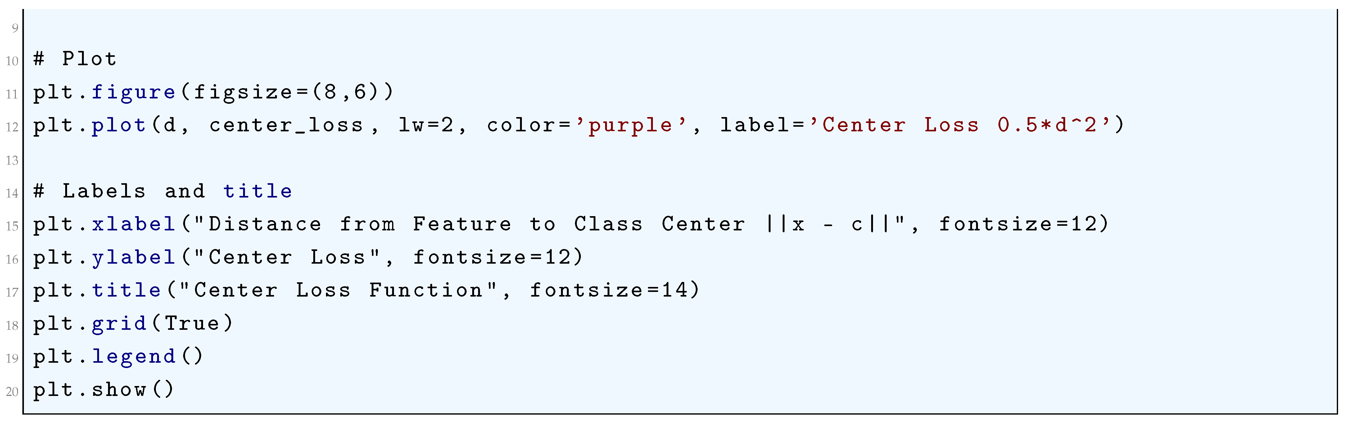
10.5.3.22 Python Code to Generate Figure 89 Illustrating Center Loss Visualization: Features vs Class Centers
The Python code below produces the Figure 89 illustrating Center Loss Visualization: Features vs Class Centers.
Figure 89.
Center Loss Visualization: Features vs Class Centers
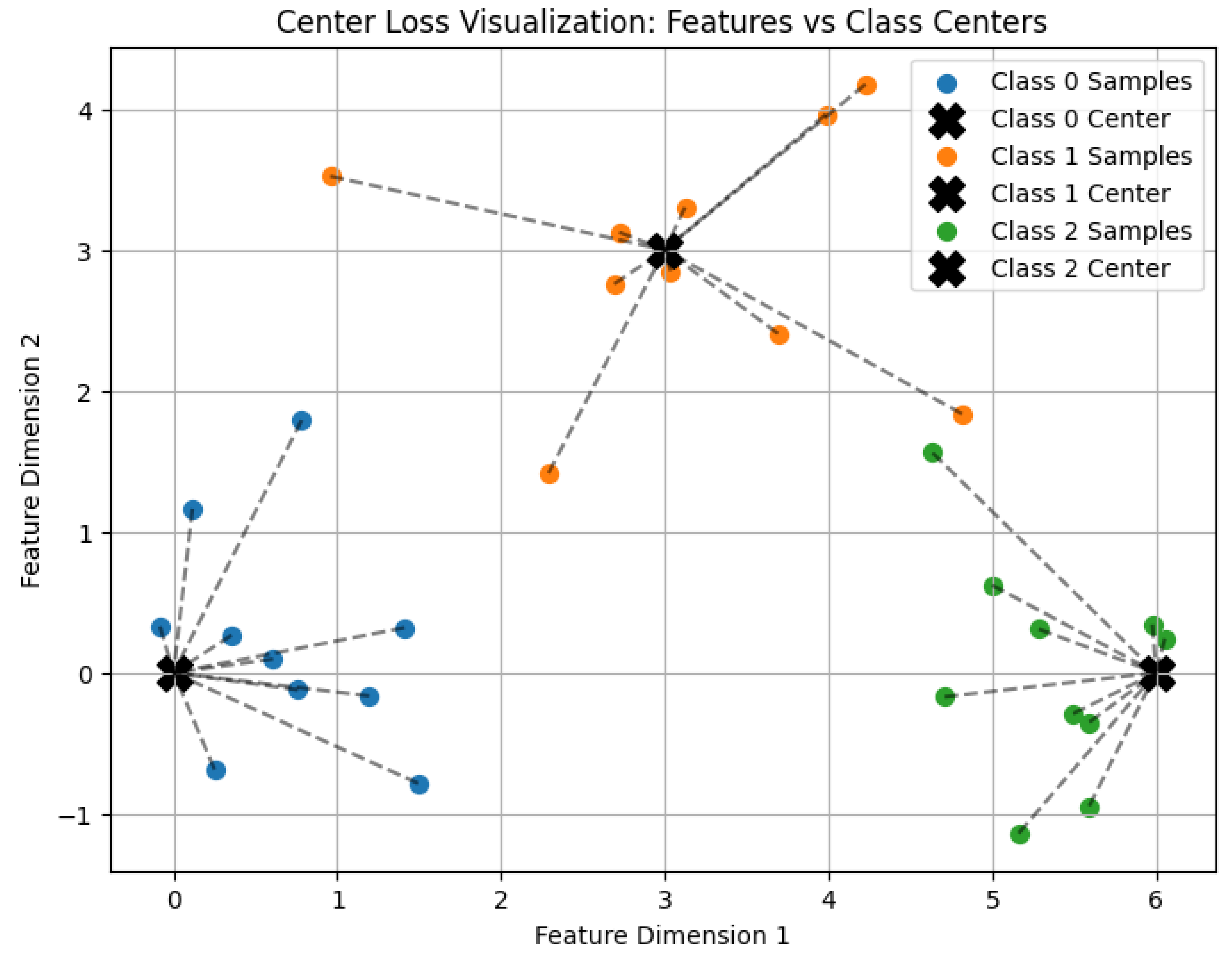
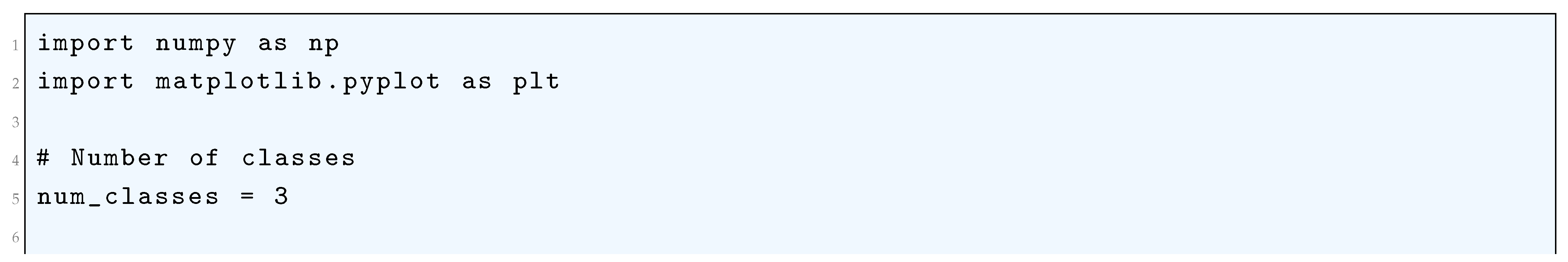
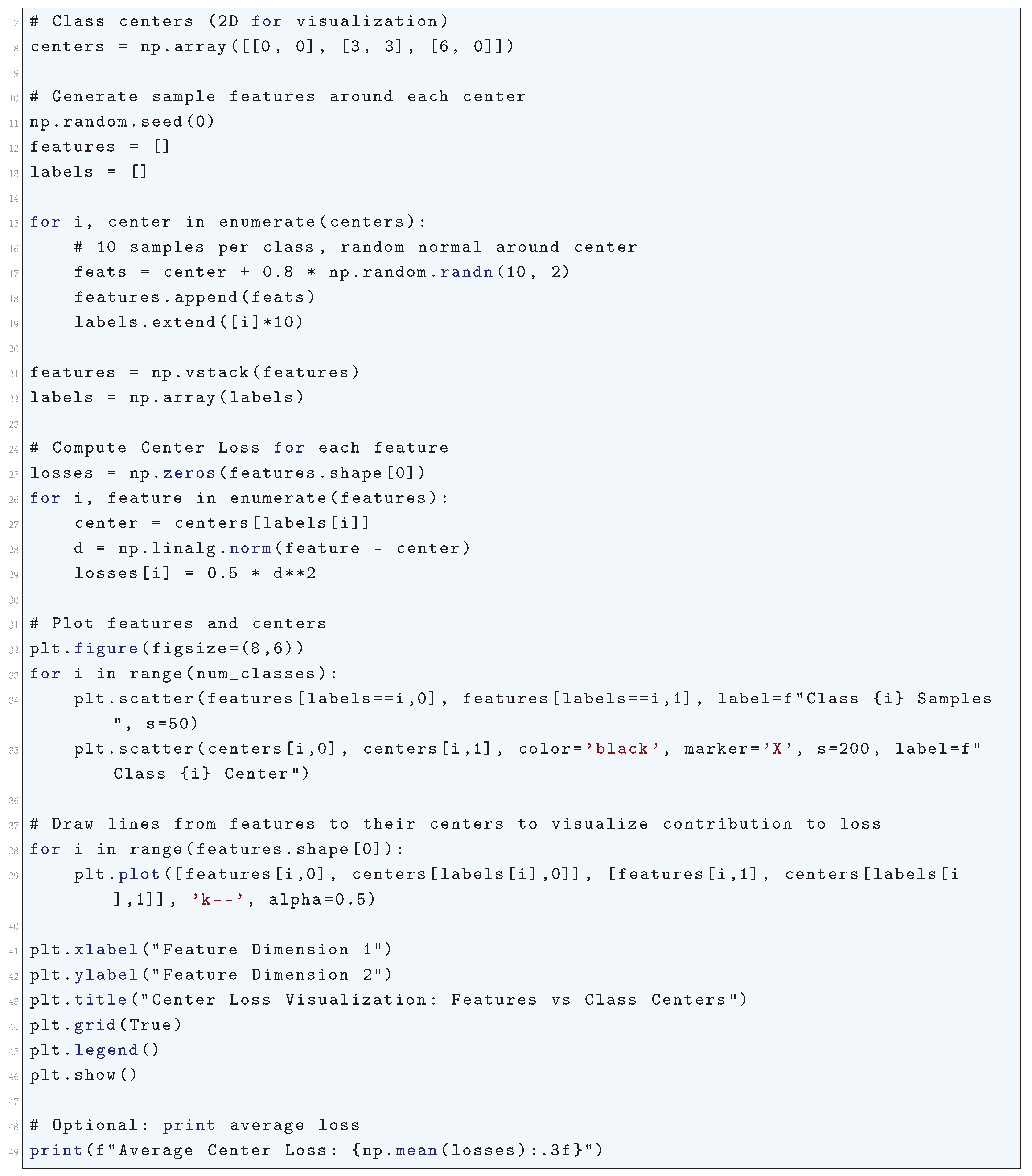
10.5.3.23 Python Code to Generate Figure 90 Illustrating 3D Center Loss Surface
The Python code below produces the Figure 90 illustrating 3D Center Loss Surface.
Figure 90.
3D Center Loss Surface
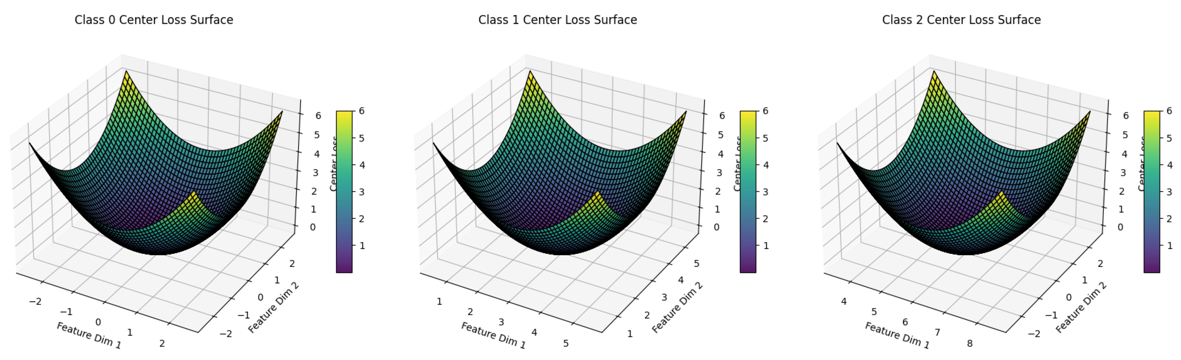
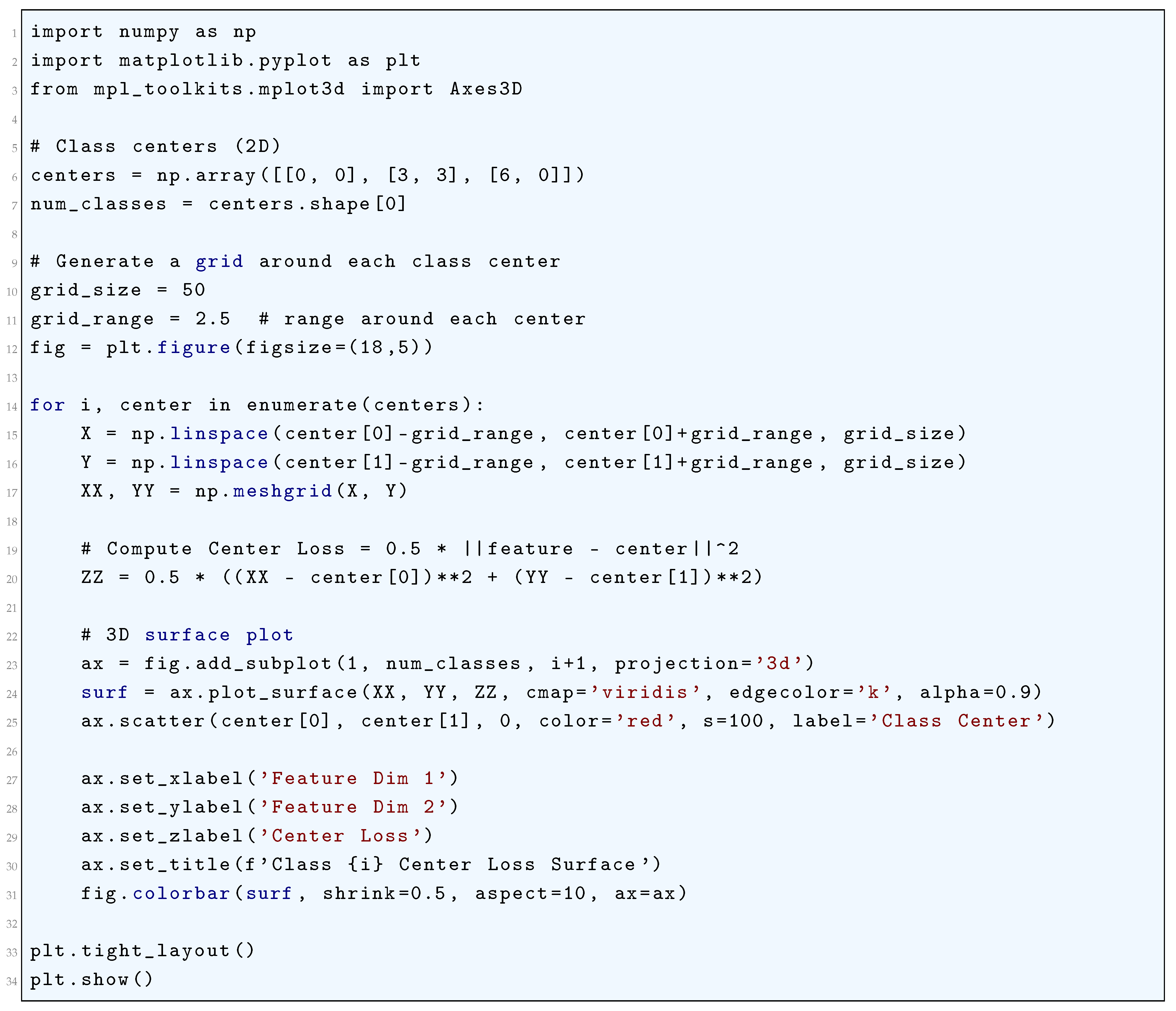
10.5.3.24 Python Code to Generate Figure 91 Illustrating Perceptual Loss Function
The Python code below produces the Figure 91 illustrating Perceptual Loss Function.
Figure 91.
Perceptual Loss Function
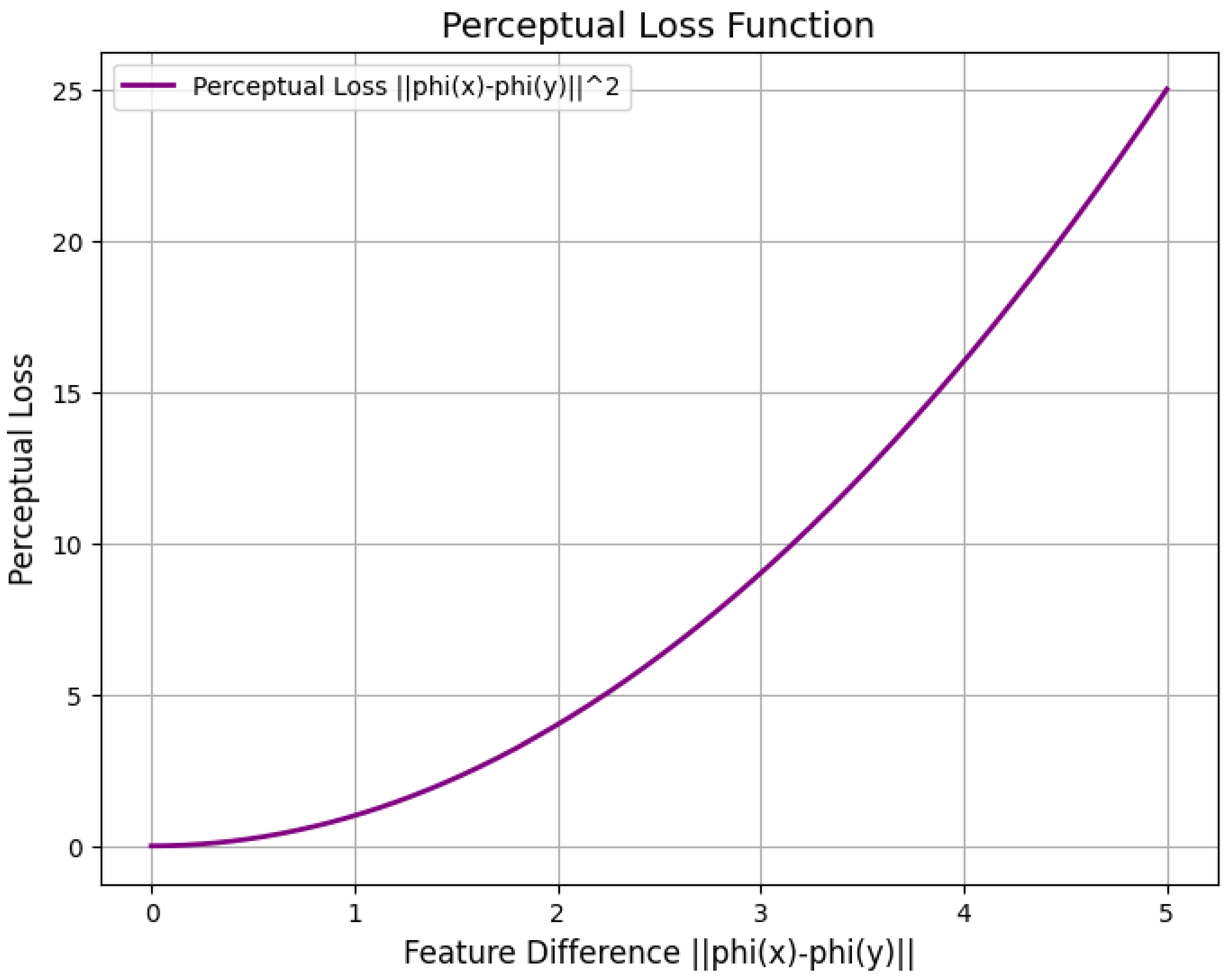
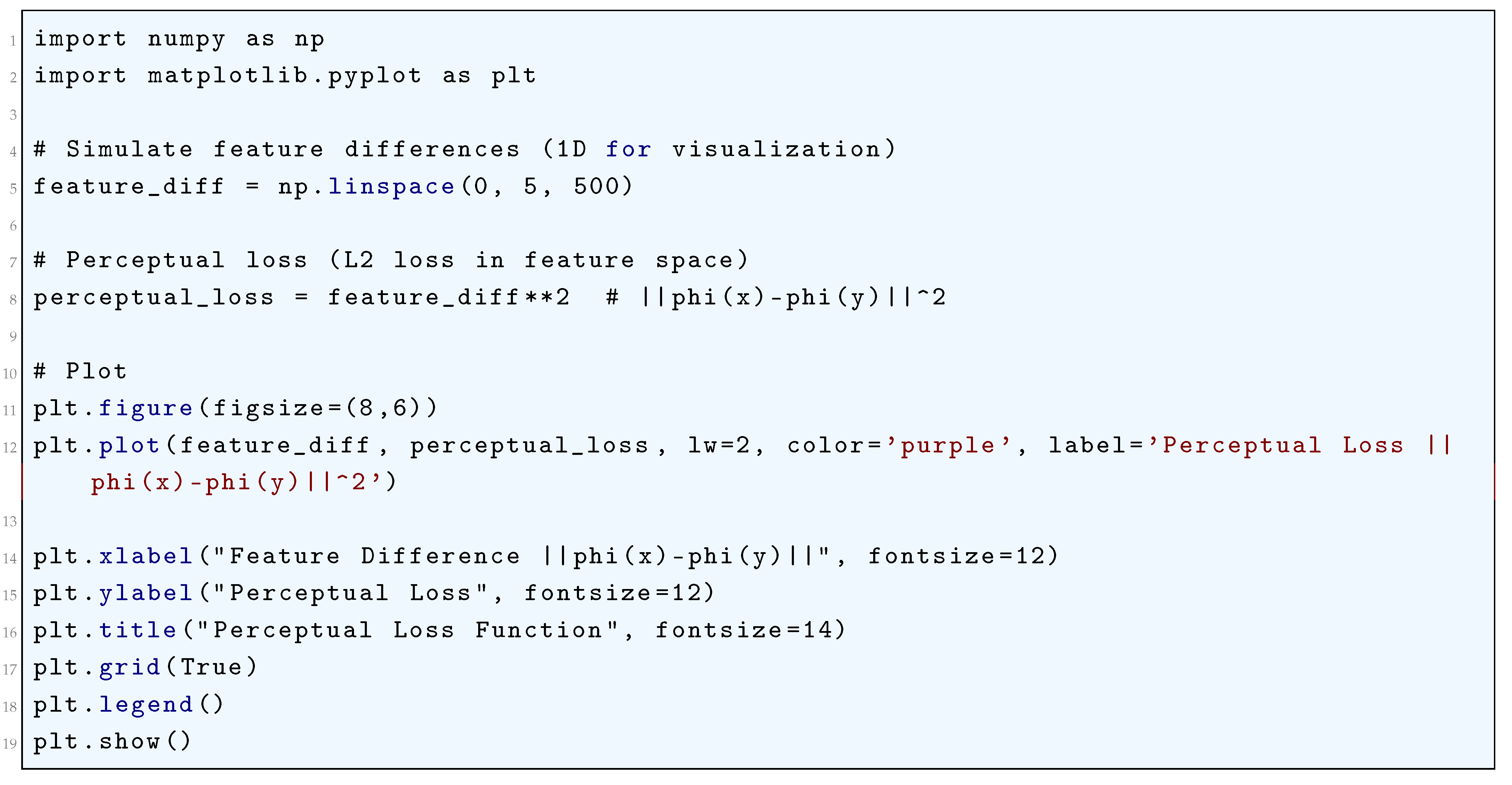
10.5.3.25 Python Code to Generate Figure 92 Illustrating Pixel-Wise MSE vs Perceptual Loss (Nonlinear Features)
The Python code below produces the Figure 92 illustrating Pixel-wise MSE vs Perceptual Loss (Nonlinear Features).
Figure 92.
Pixel-wise MSE vs Perceptual Loss (Nonlinear Features)
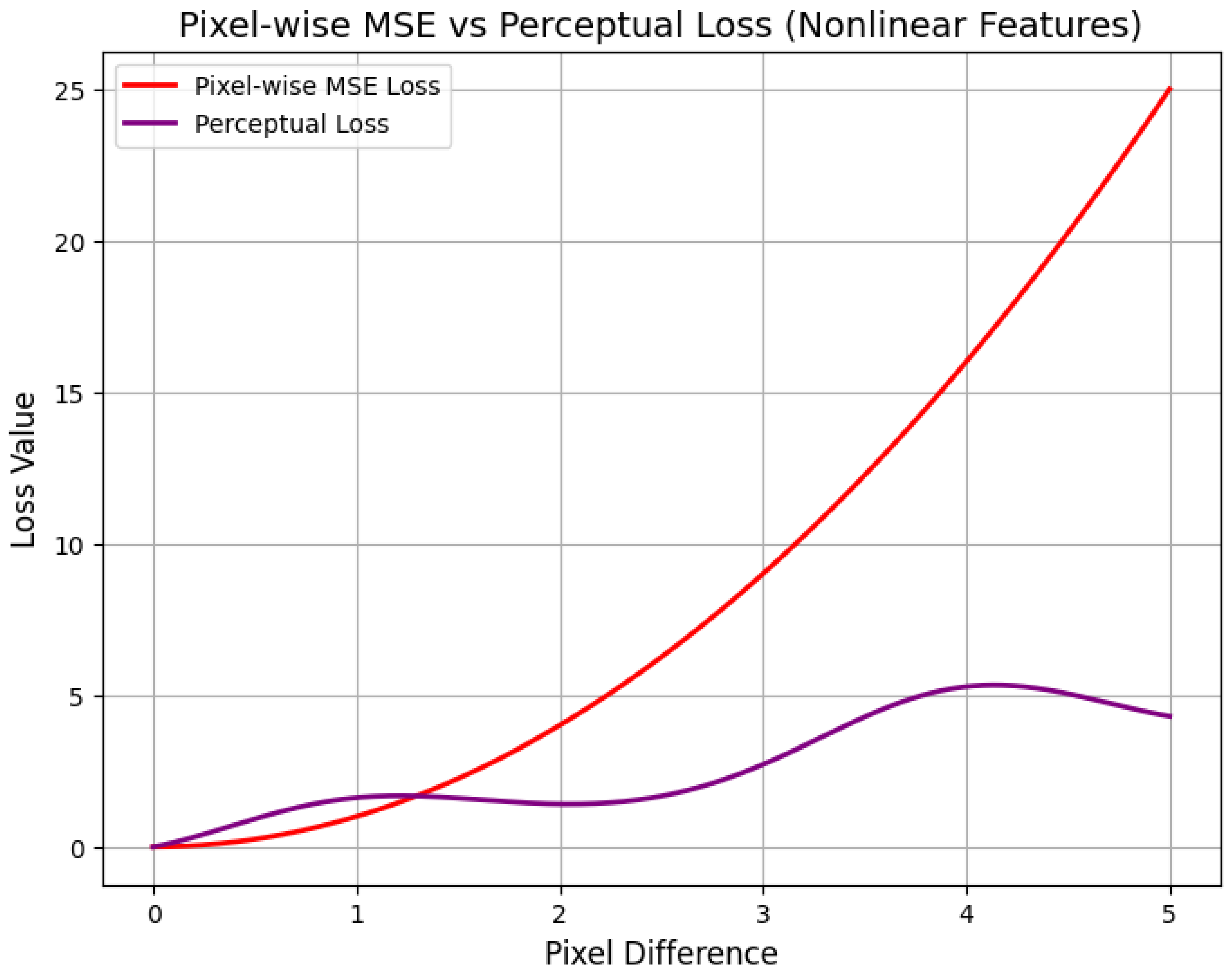
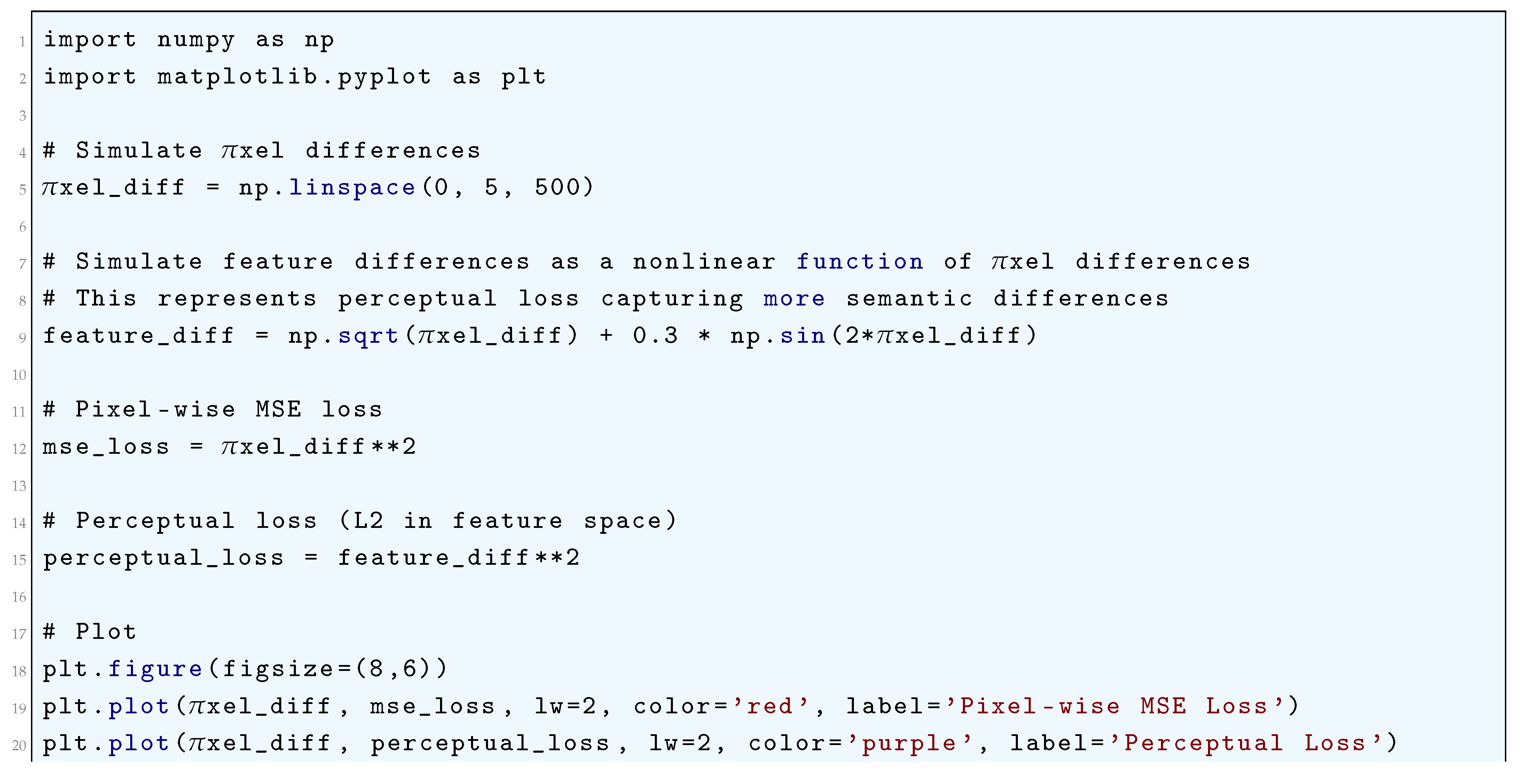
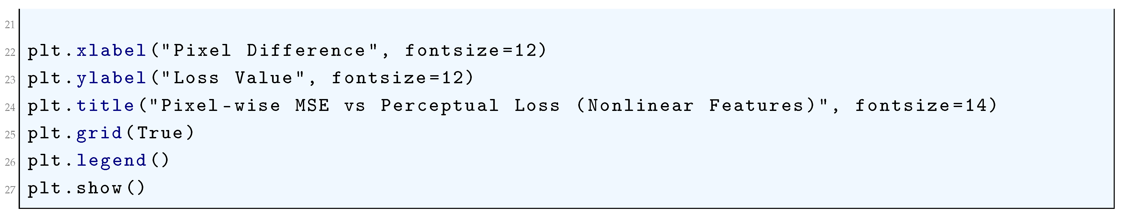
10.5.3.26 Python Code to Generate Figure 93 Illustrating Style Loss Function in Neural Style Transfer
The Python code below produces the Figure 93 illustrating Style Loss Function in Neural Style Transfer.
Figure 93.
Style Loss Function in Neural Style Transfer
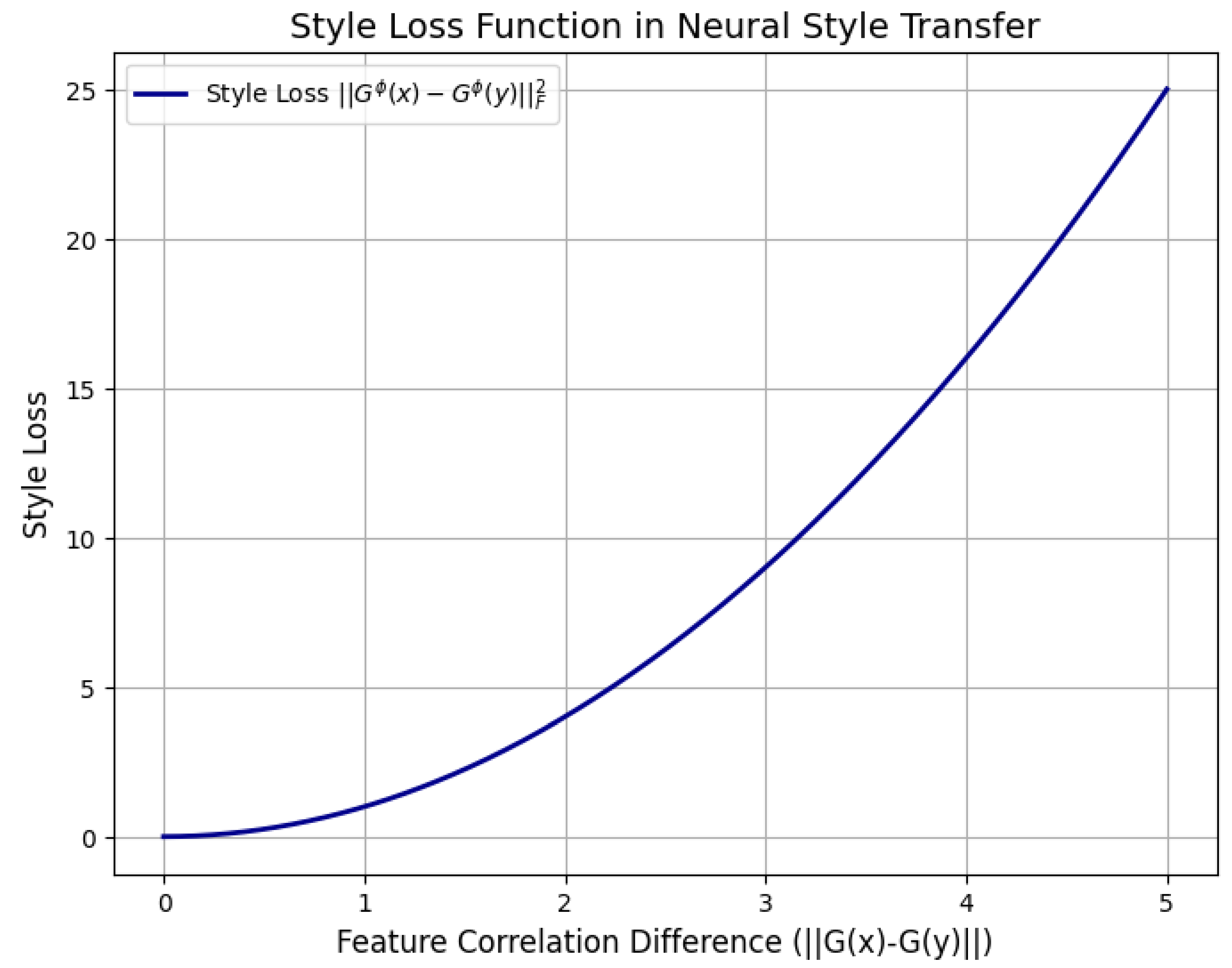
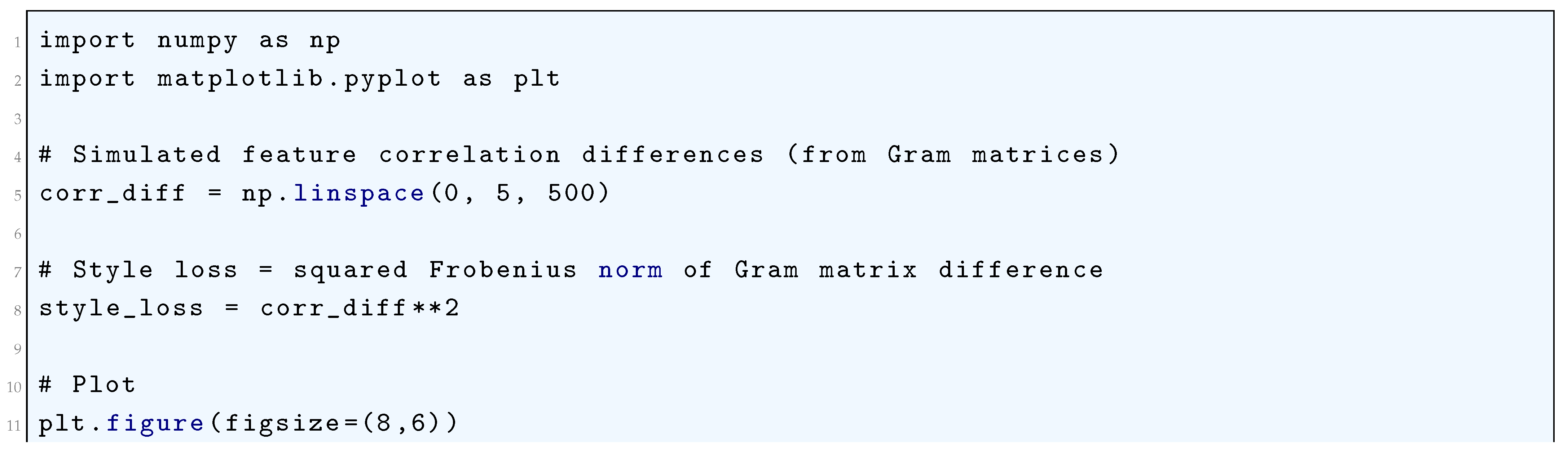
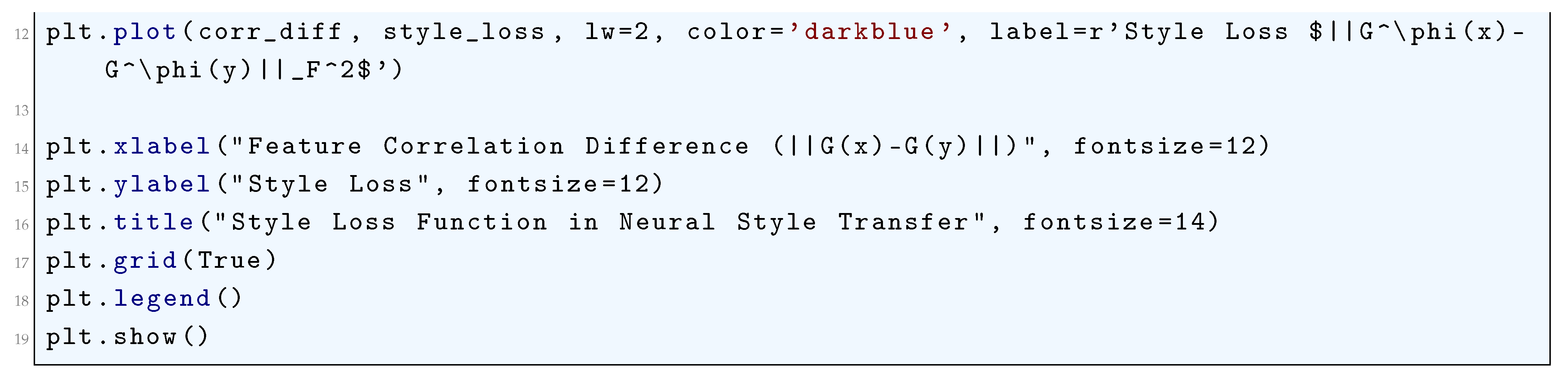
10.5.3.27 Python Code to Generate Figure 94 Illustrating Style Loss vs Scaling of Generated Features
The Python code below produces the Figure 94 illustrating Style Loss vs Scaling of Generated Features.
Figure 94.
Style Loss vs Scaling of Generated Features
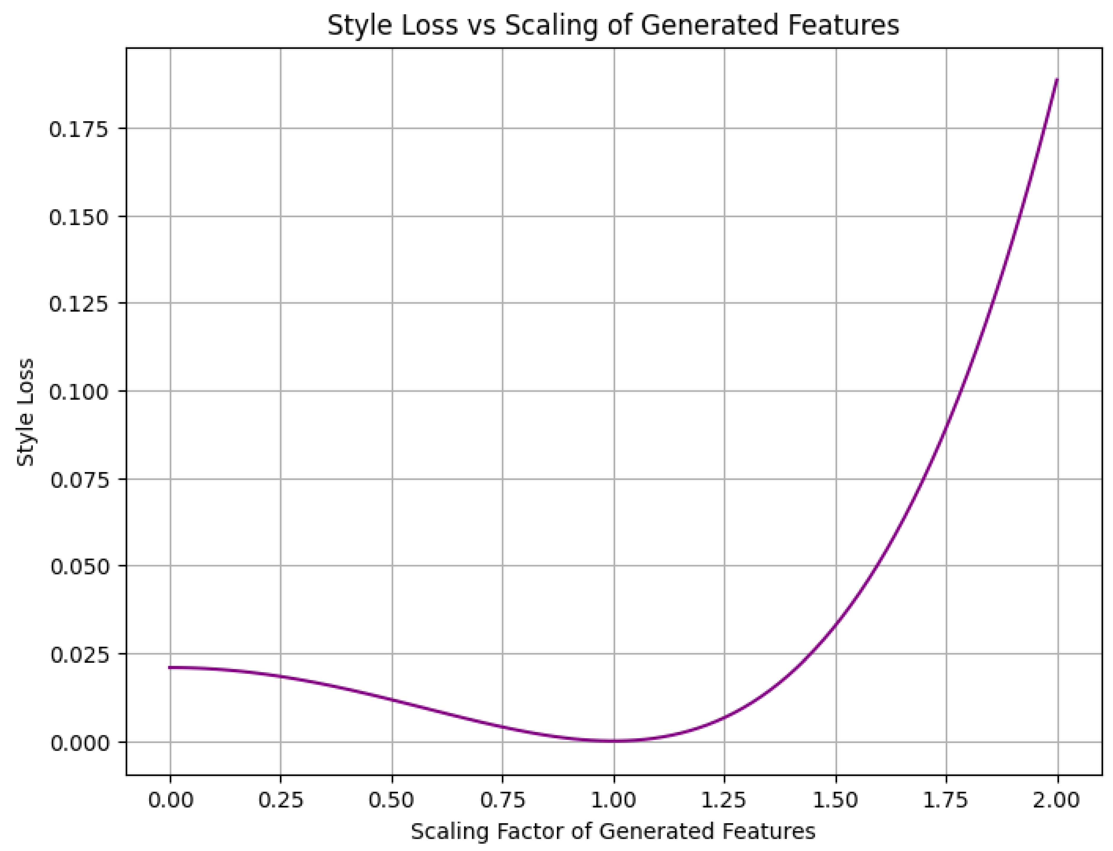
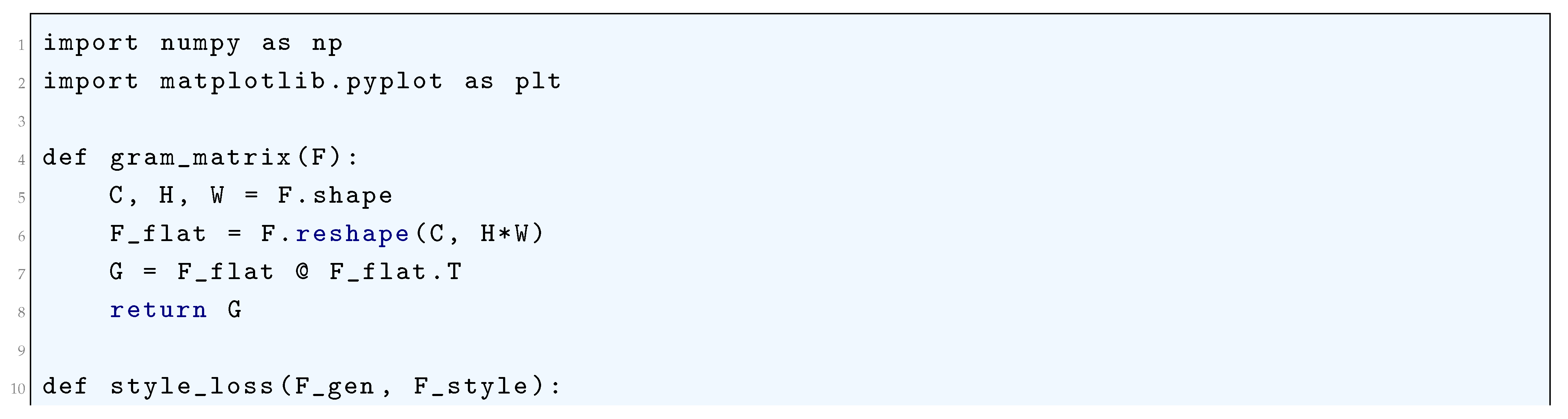
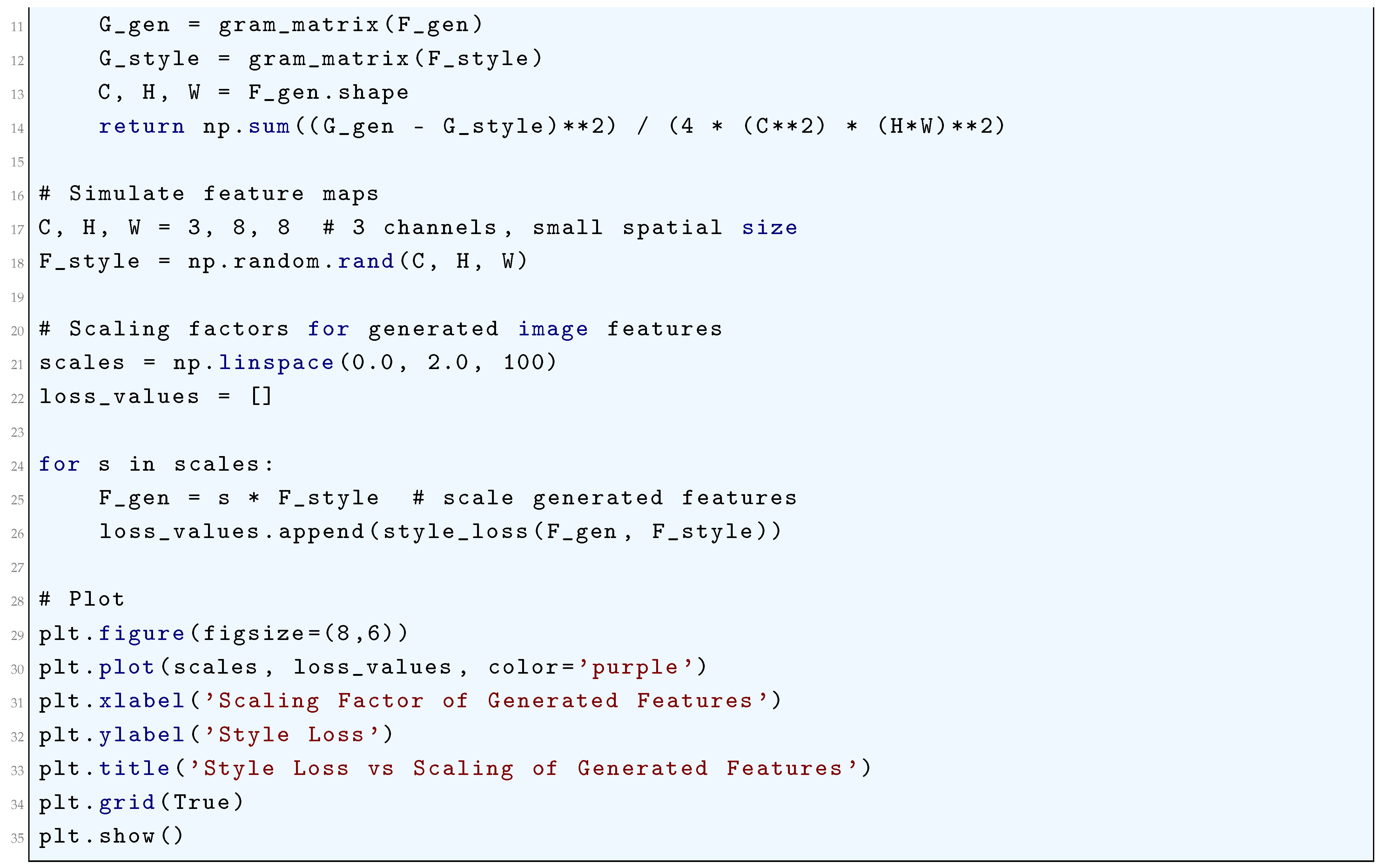
10.5.3.28 Python Code to Generate Figure 95 Illustrating Total Variation (TV) Loss
The Python code below produces the Figure 95 illustrating Total Variation (TV) Loss.
Figure 95.
Total Variation (TV) Loss
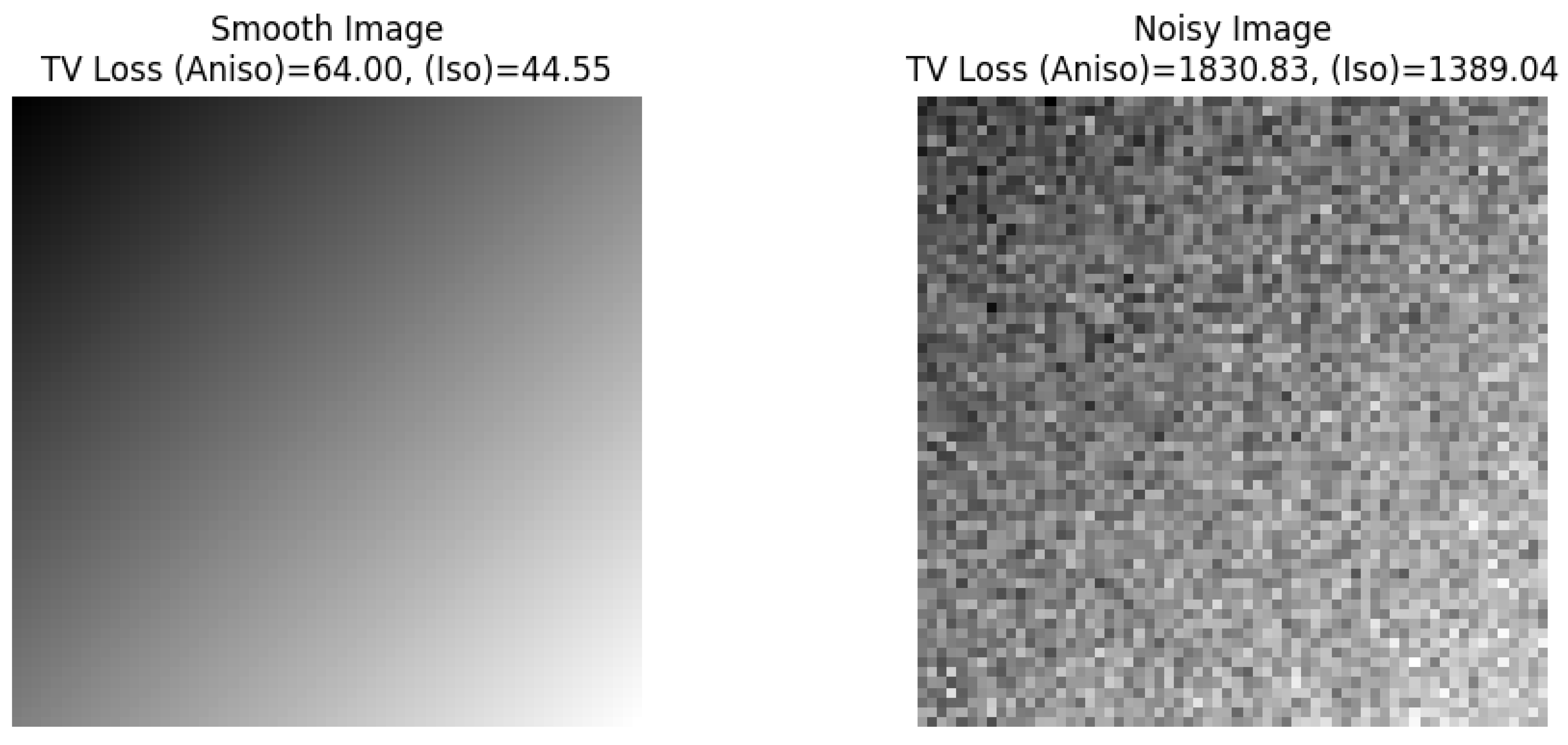

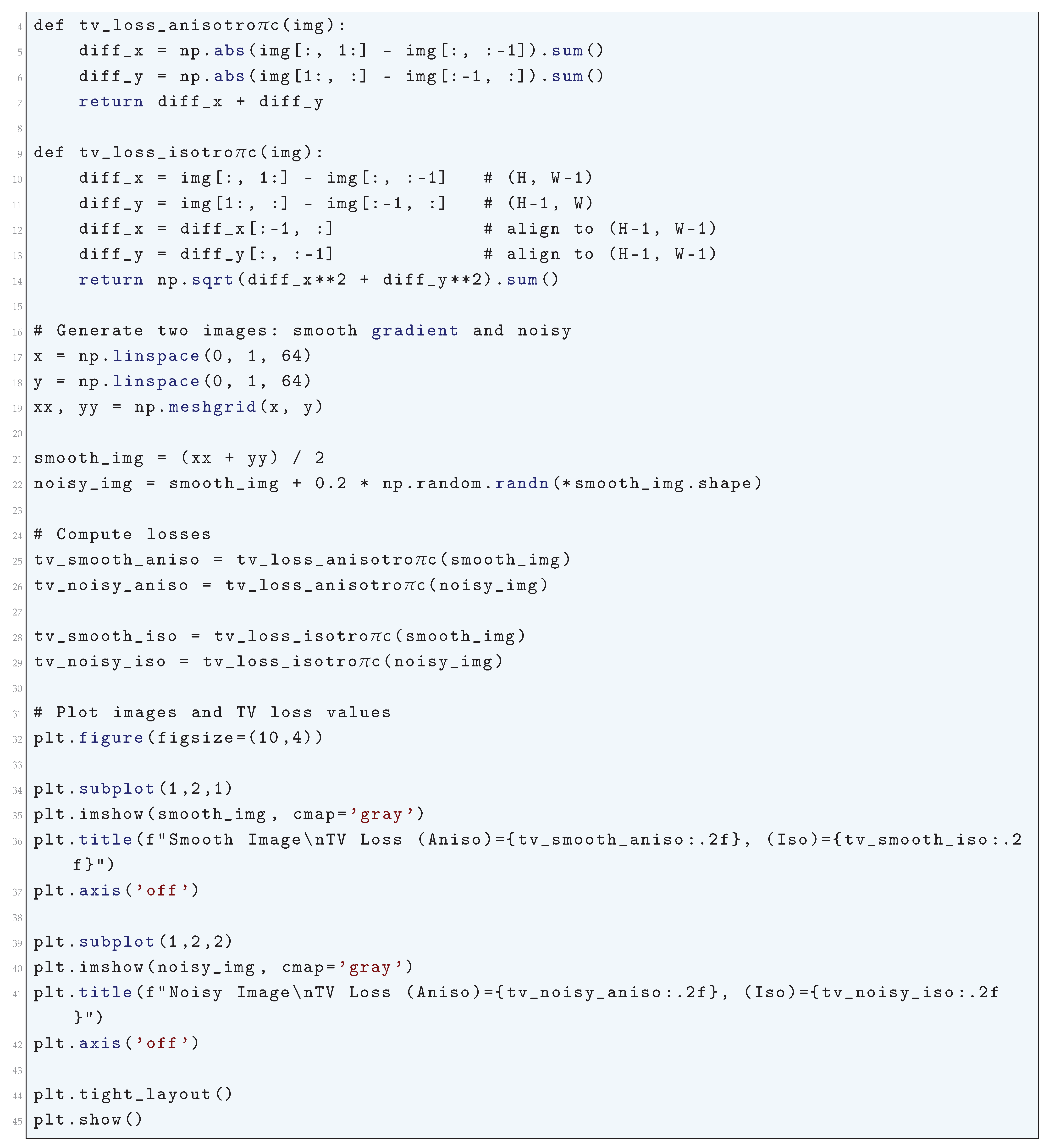
10.5.3.29 Python Code to Generate Figure 96 Illustrating Total Variation Loss vs Noise Level
The Python code below produces the Figure 96 illustrating Total Variation Loss vs Noise Level.
Figure 96.
Total Variation Loss vs Noise Level
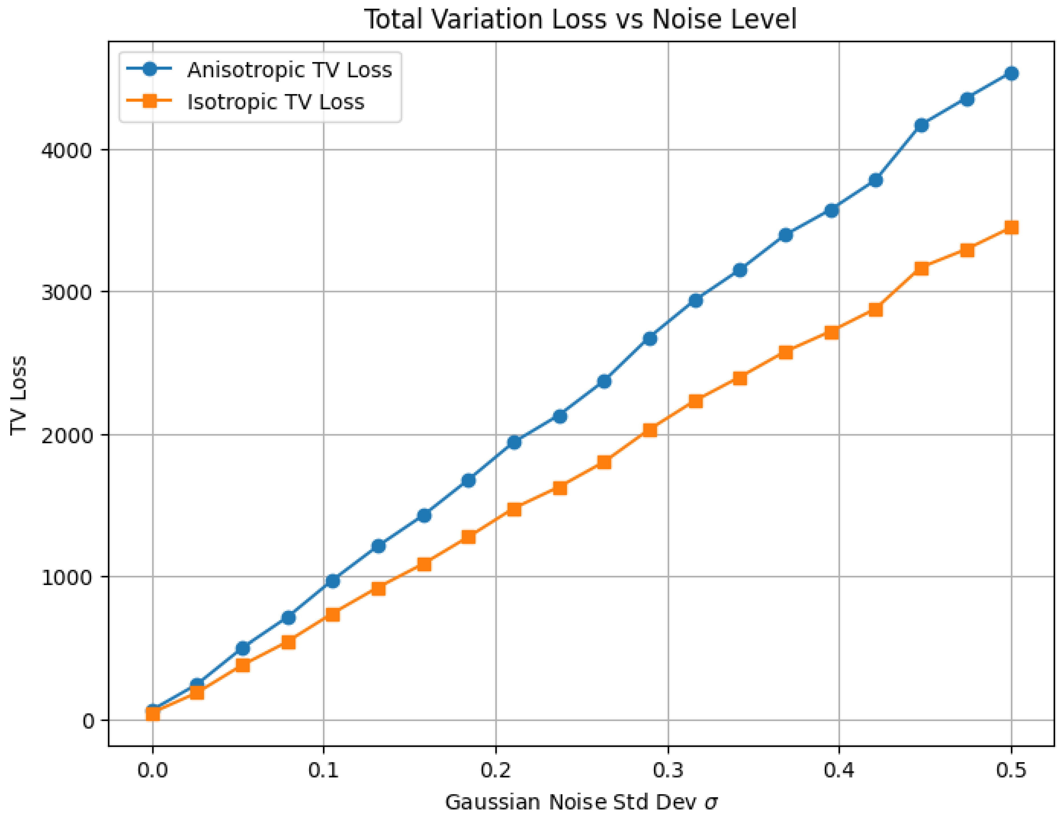
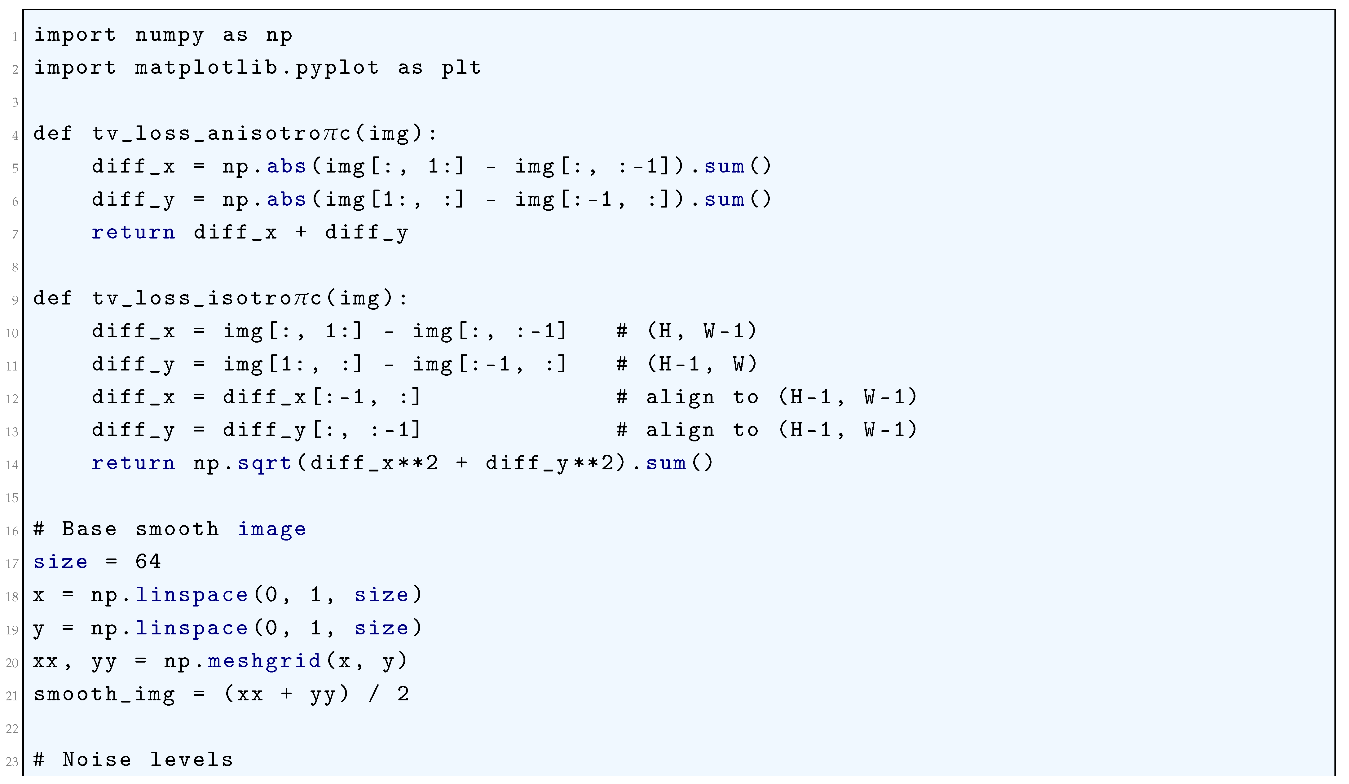
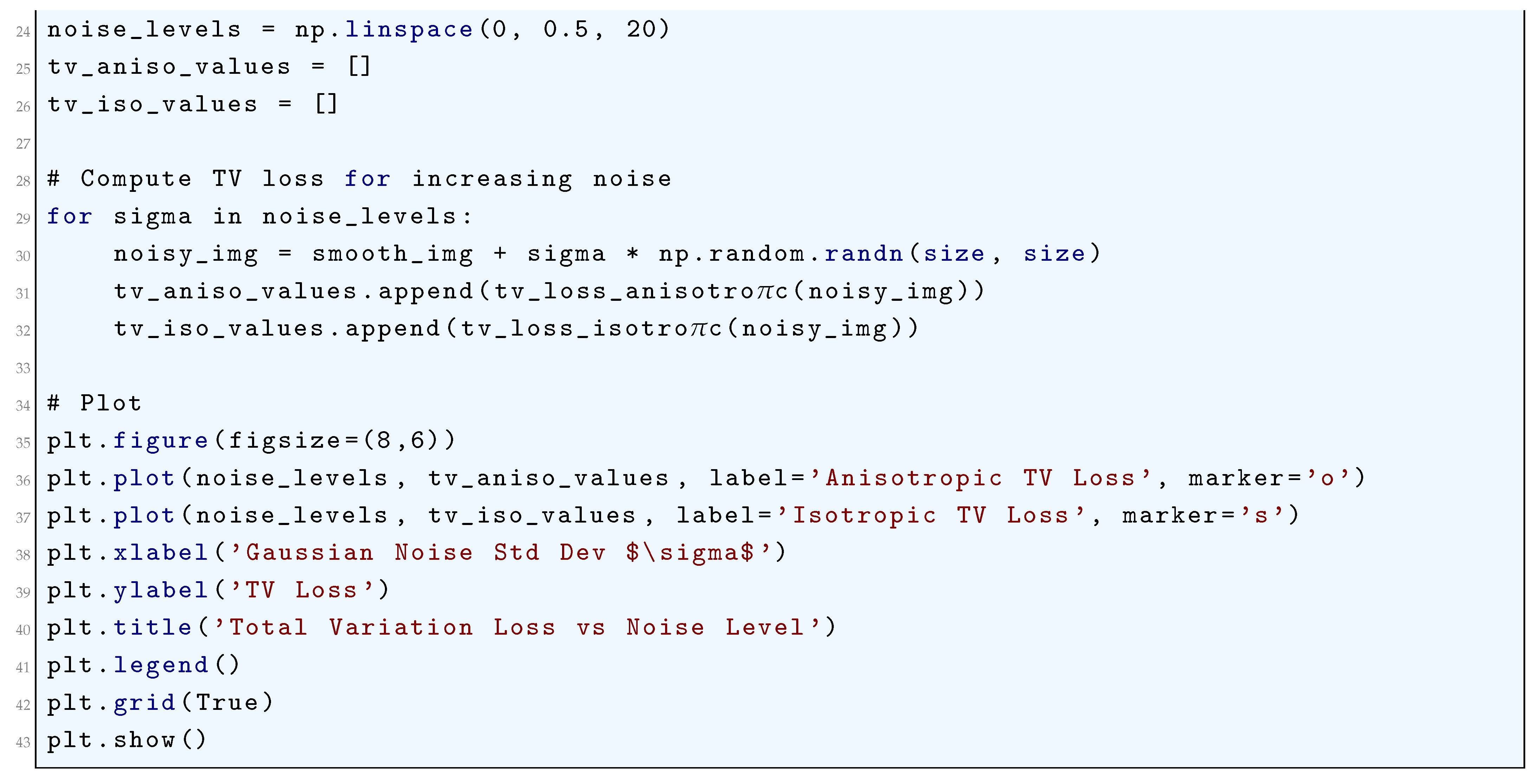
10.5.3.30 Python Code to Generate Figure 97 Illustrating Evidence Lower Bound (ELBO) Loss During Training
The Python code below produces the Figure 97 illustrating Evidence Lower Bound (ELBO) Loss during Training.
Figure 97.
Evidence Lower Bound (ELBO) Loss during Training
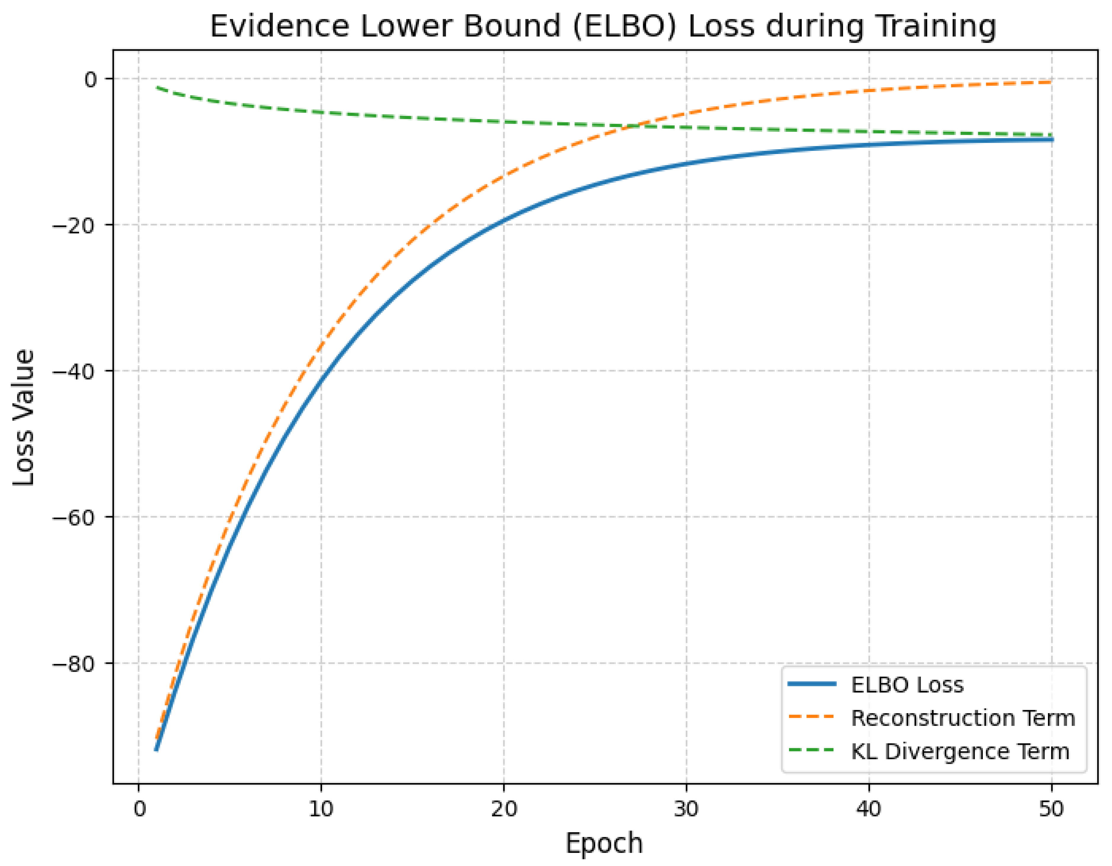
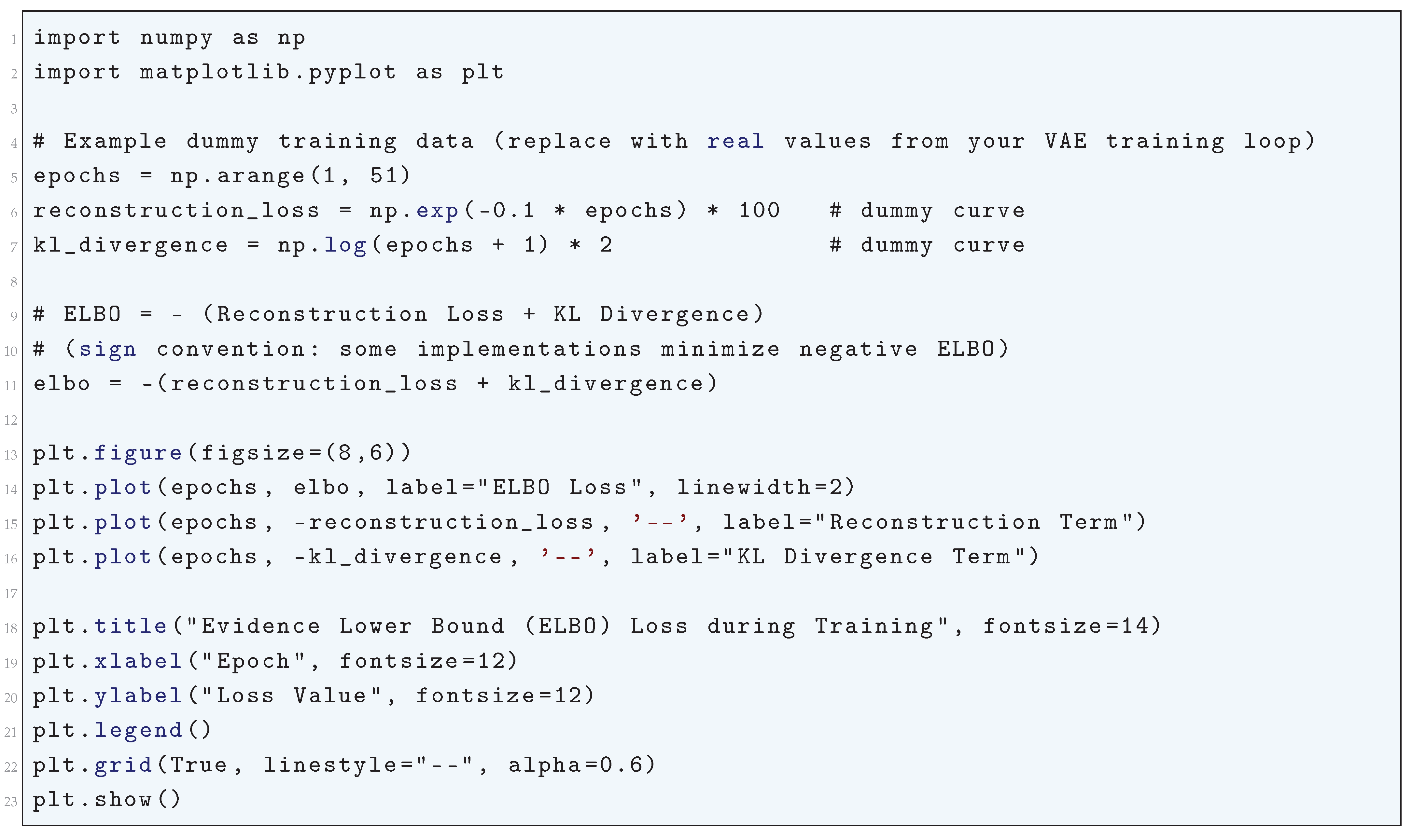
10.5.3.31 Python Code to Generate Figure 98 Illustrating Negative Log-Likelihood (NLL) Loss
The Python code below produces the Figure 98 illustrating Negative Log-Likelihood (NLL) Loss.
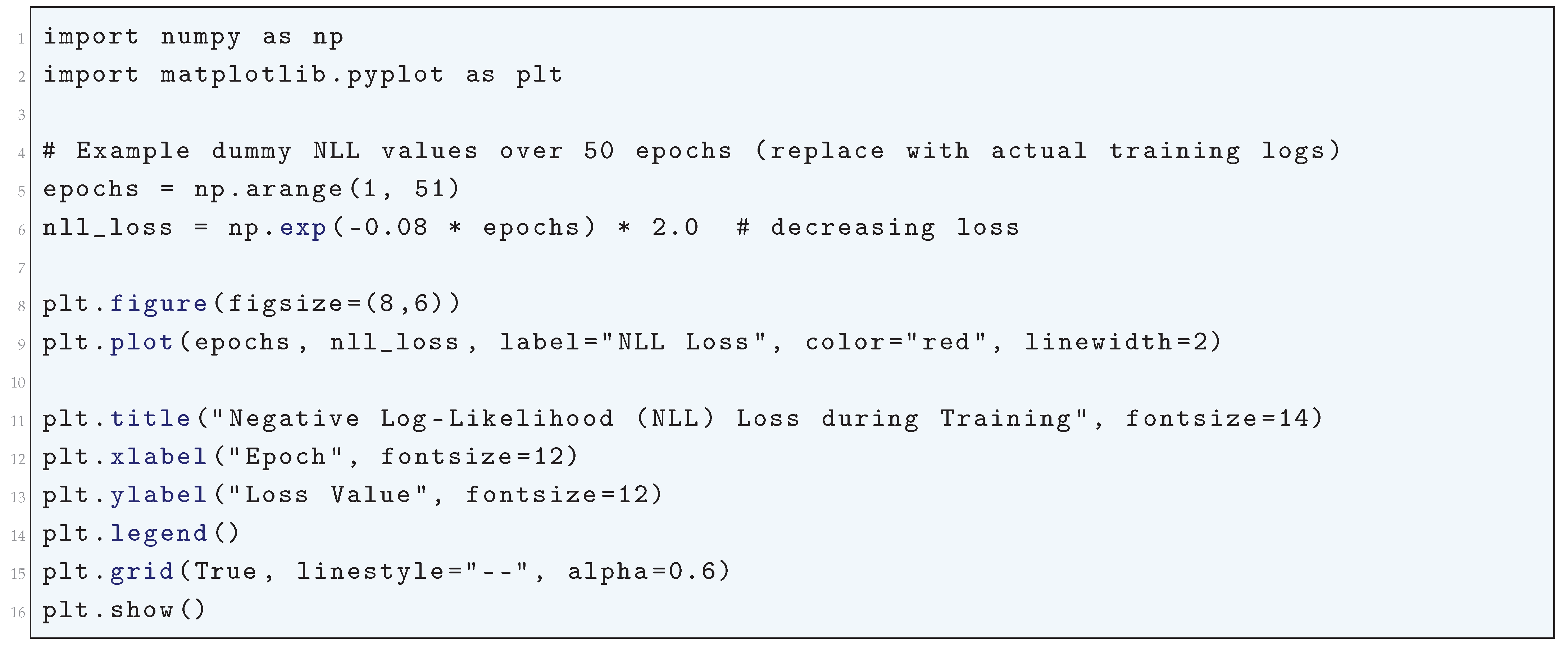
Figure 98.
Negative Log-Likelihood (NLL) Loss during Training
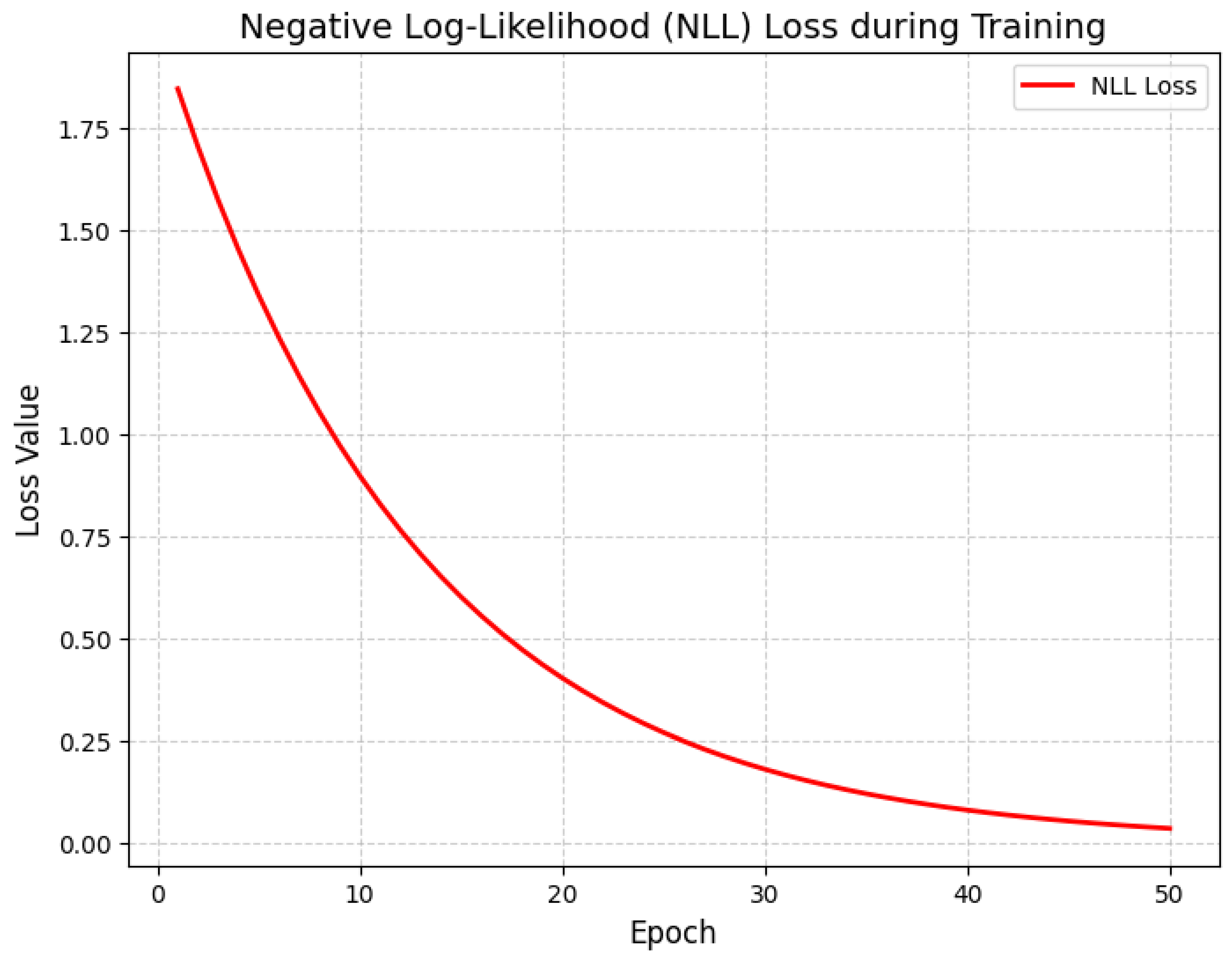
10.5.3.32 Python Code to Generate Figure 99 Illustrating Domain Adversarial Loss During Training
The Python code below produces the Figure 99 illustrating Domain Adversarial Loss during Training.
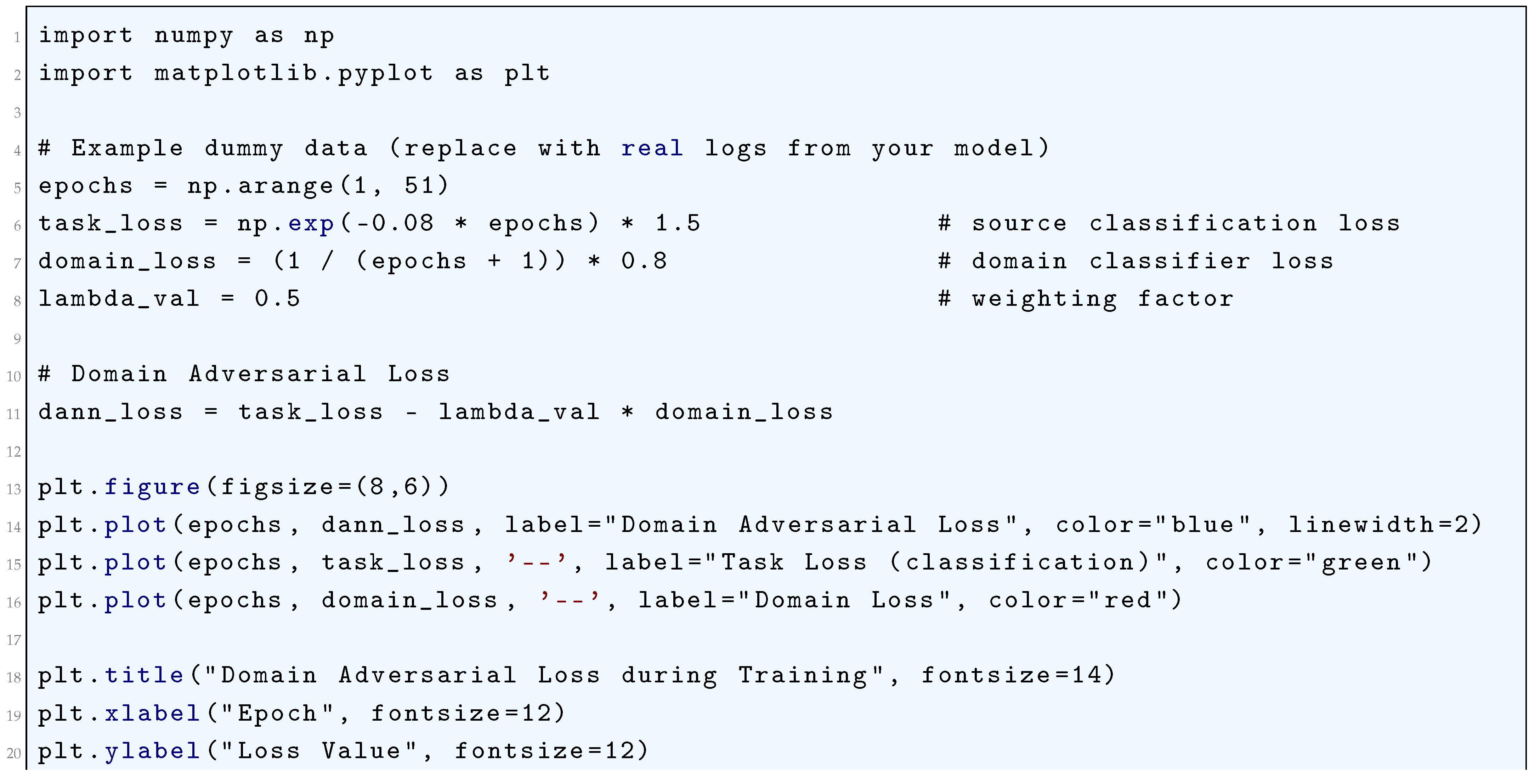

Figure 99.
Domain Adversarial Loss during Training
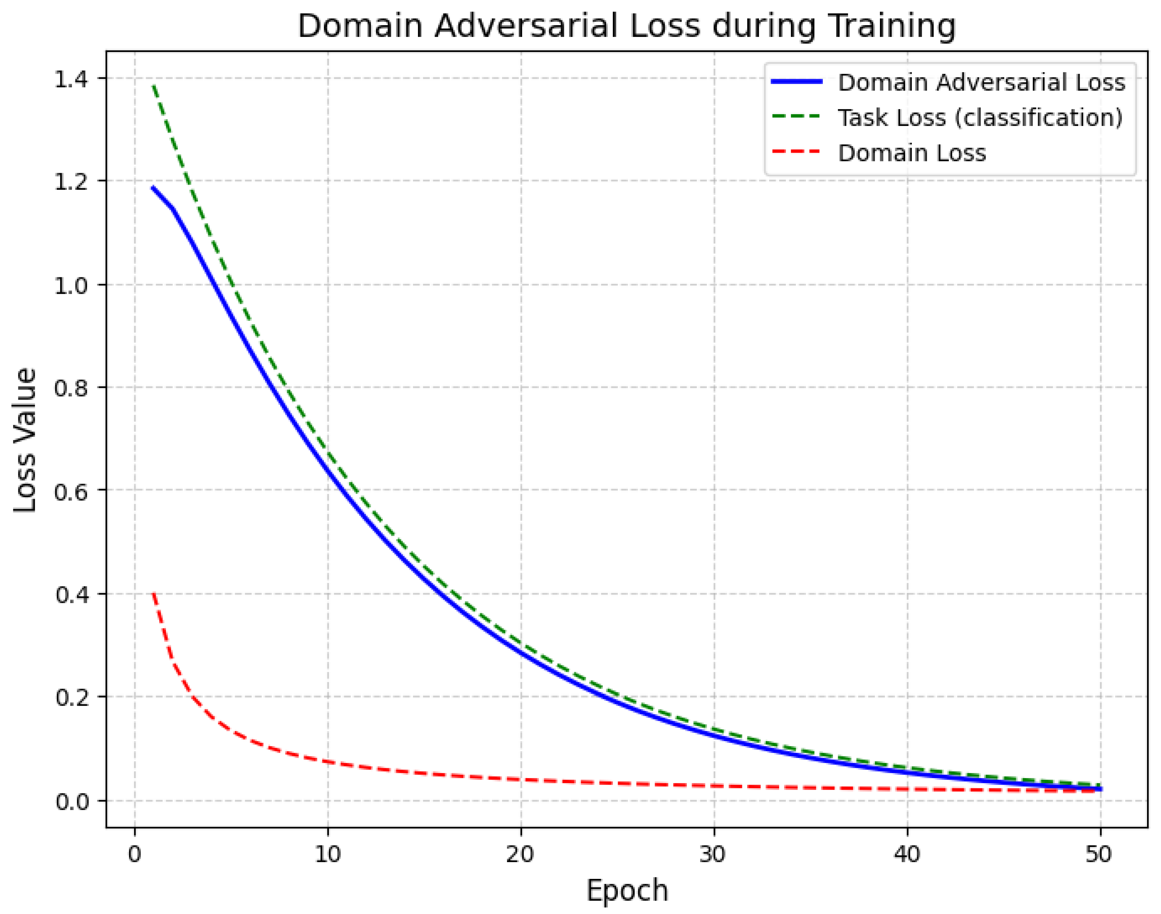
10.5.3.33 Python Code to Generate Figure 100 Illustrating Maximum Mean Discrepancy (MMD) Loss During Training
The Python code below produces the Figure 100 illustrating Maximum Mean Discrepancy (MMD) Loss during Training.
Figure 100.
Maximum Mean Discrepancy (MMD) Loss during Training
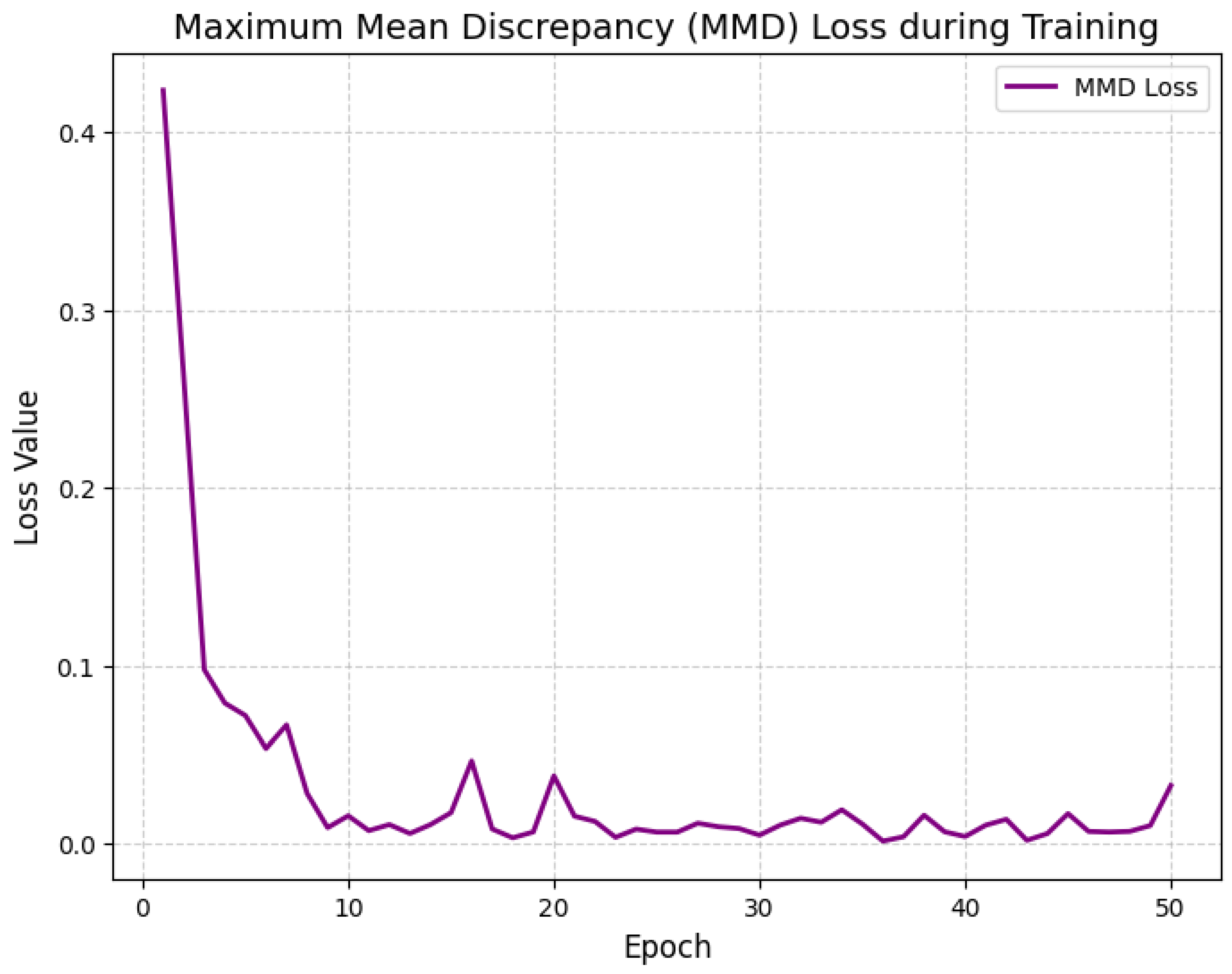
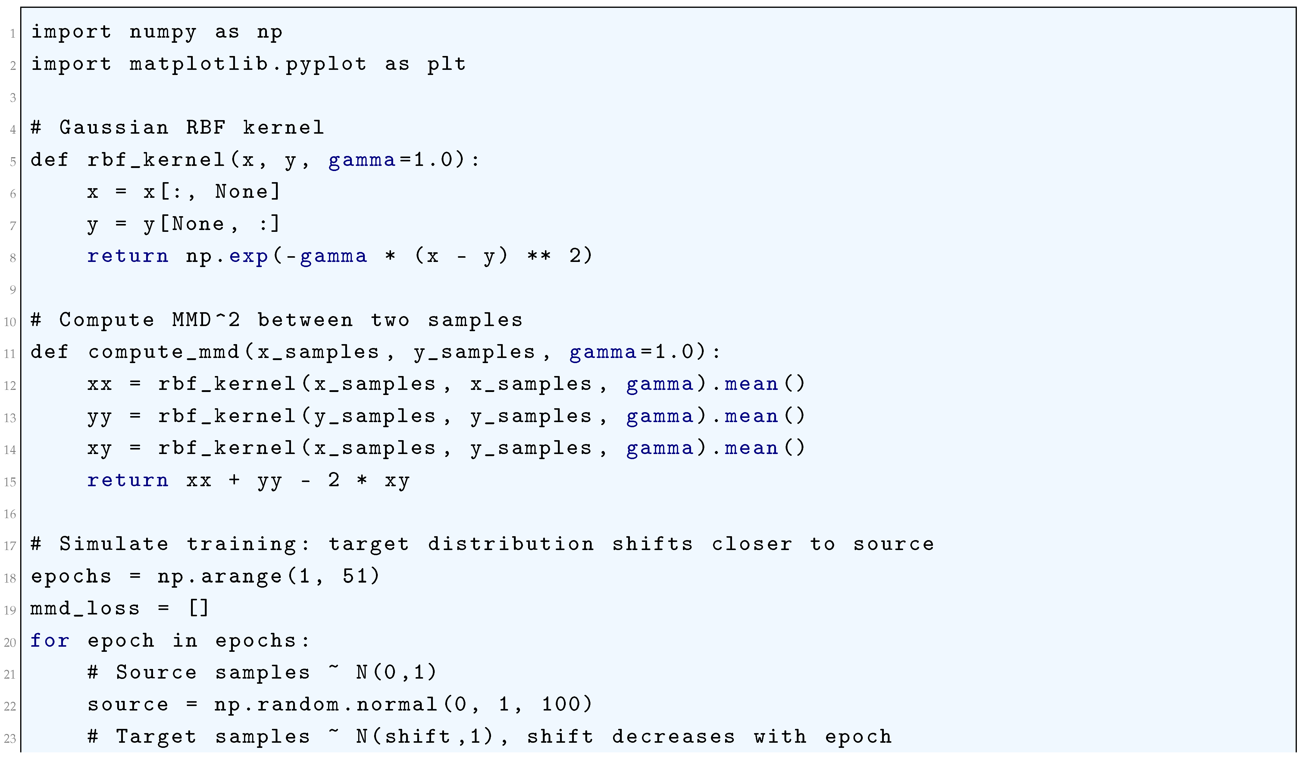
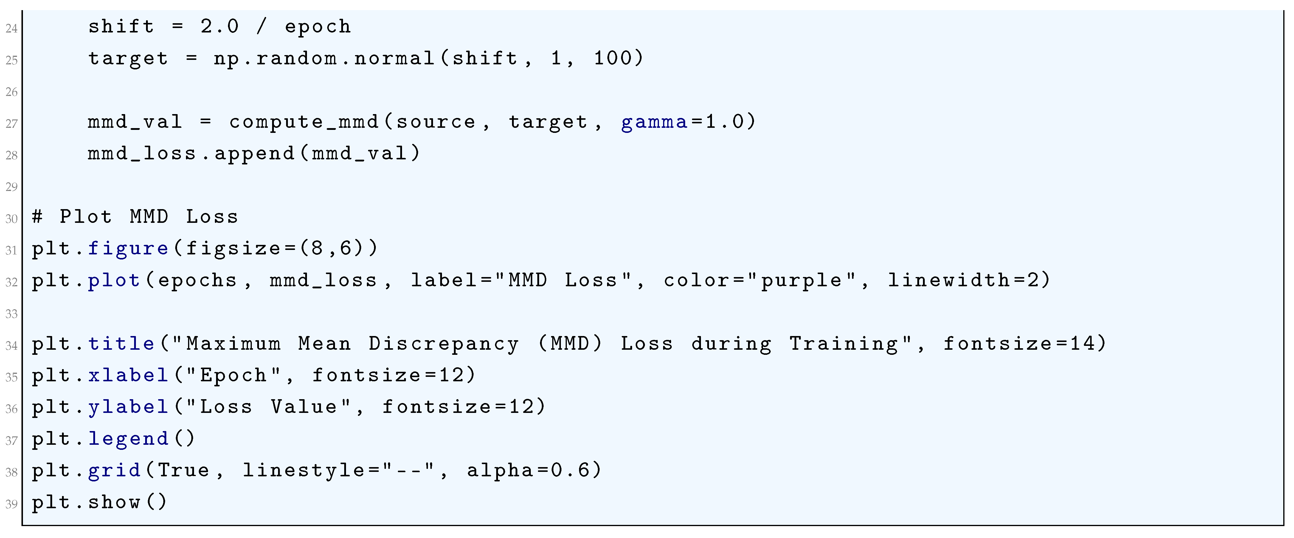
10.5.3.34 Python Code to Generate Figure 101 Illustrating IoU Loss and Variants (GIoU Loss, DIoU Loss, CIoU Loss)
The Python code below produces the Figure 101 illustrating IoU Loss and Variants (GIoU Loss, DIoU Loss, CIoU Loss).
Figure 101.
IoU Loss and Variants (GIoU Loss, DIoU Loss, CIoU Loss)
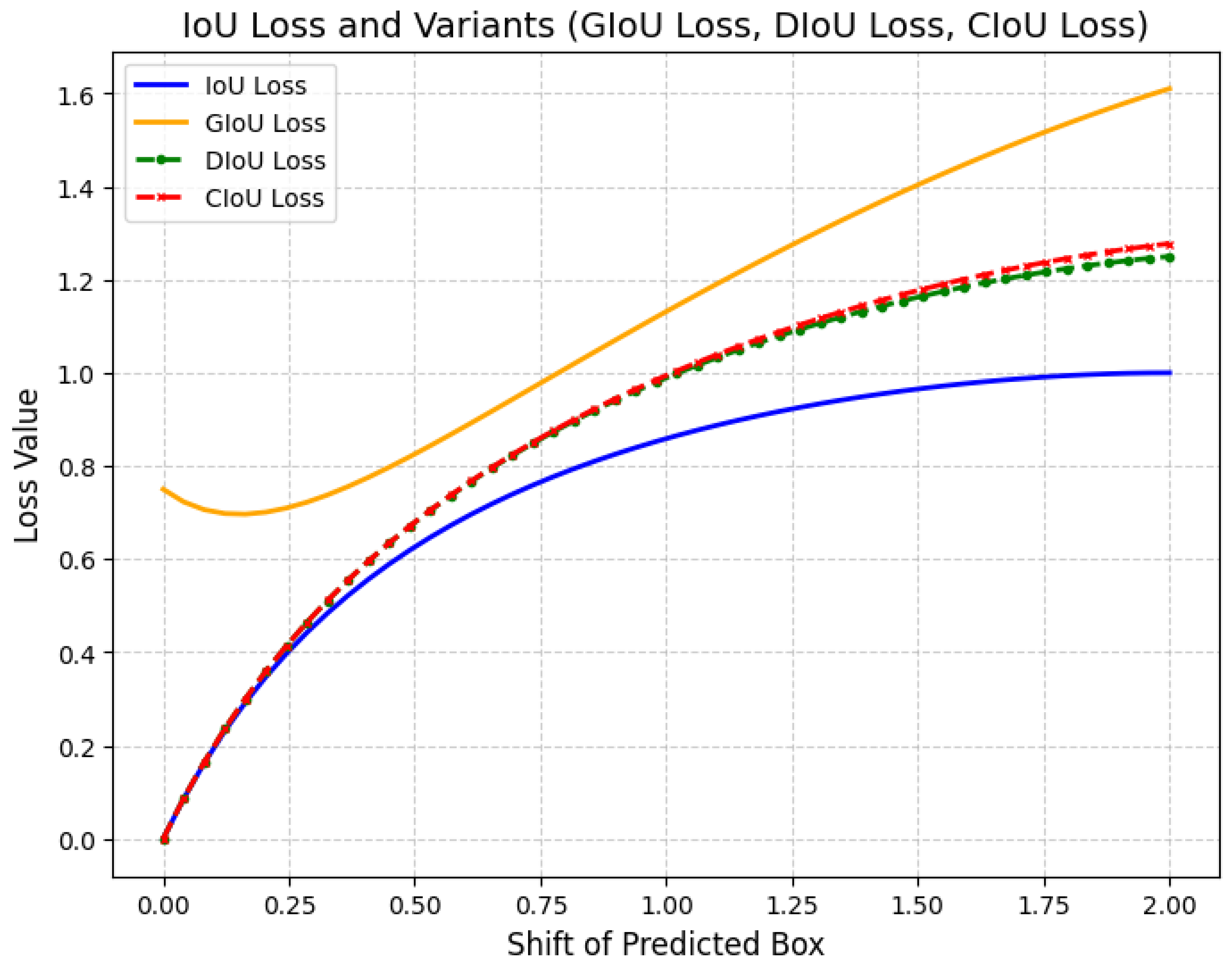
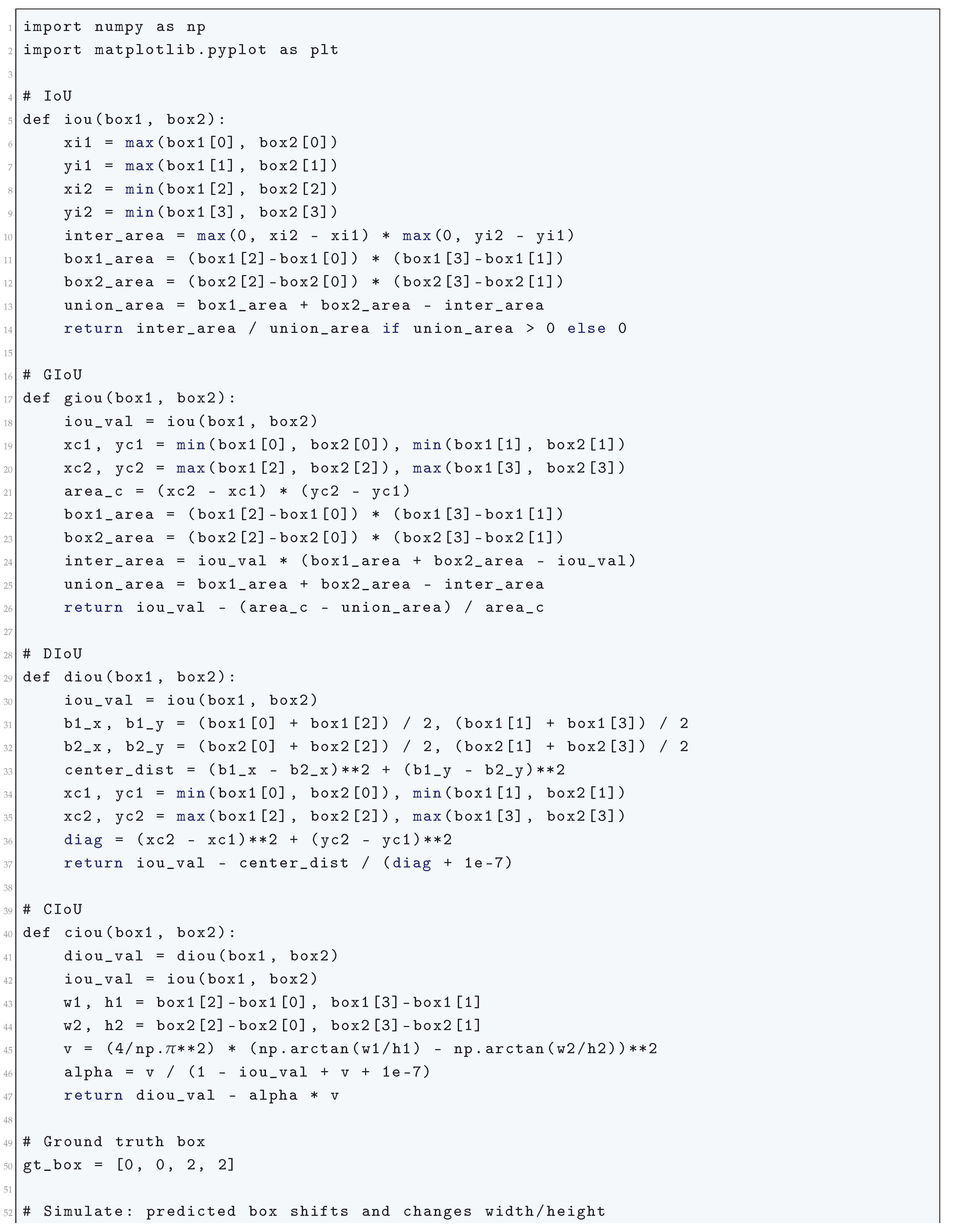
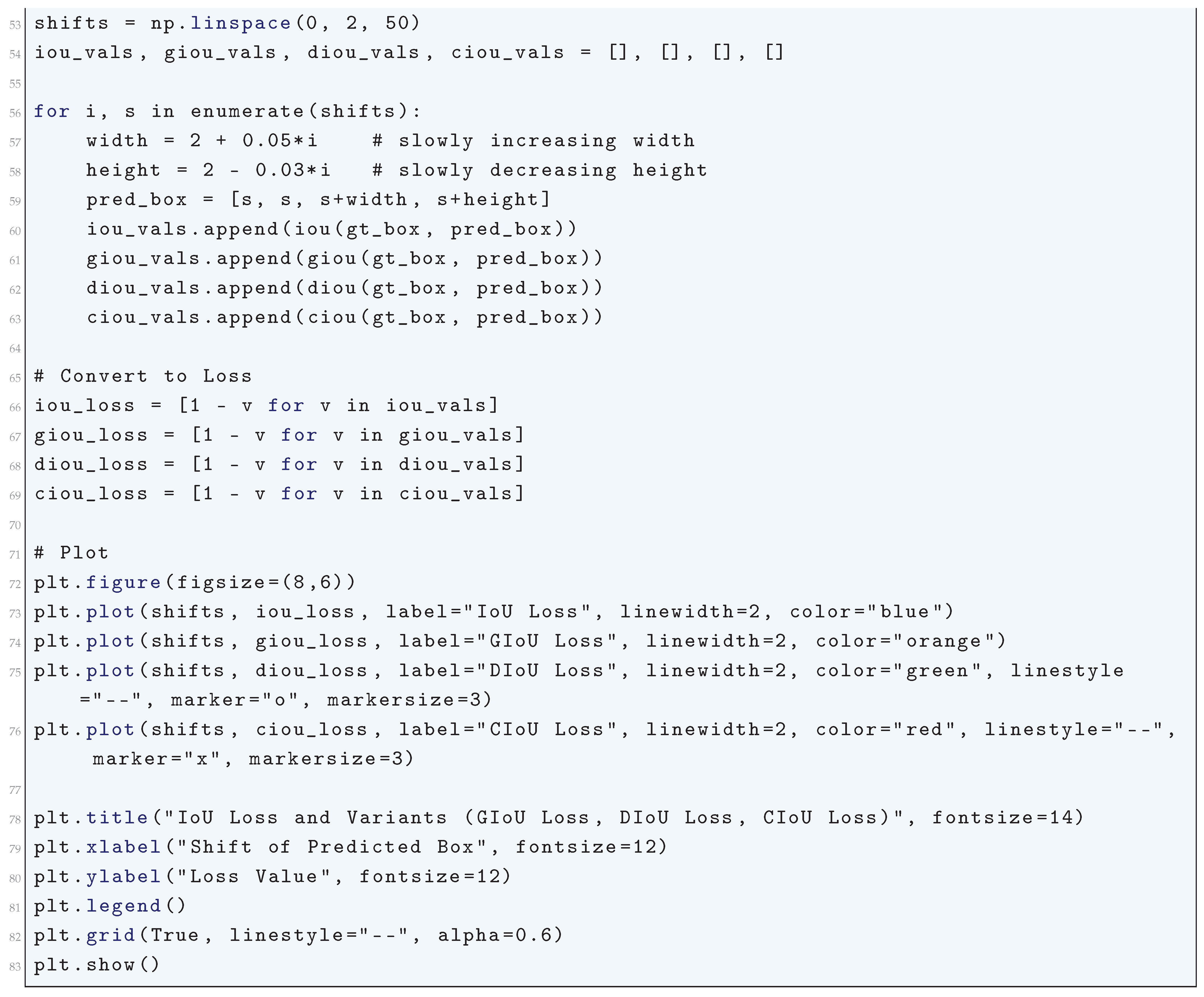
10.5.3.35 Python Code to Generate Figure 102 Illustrating Dice Loss During Training
The Python code below produces the Figure 102 illustrating Dice Loss during Training.
Figure 102.
Dice Loss during Training
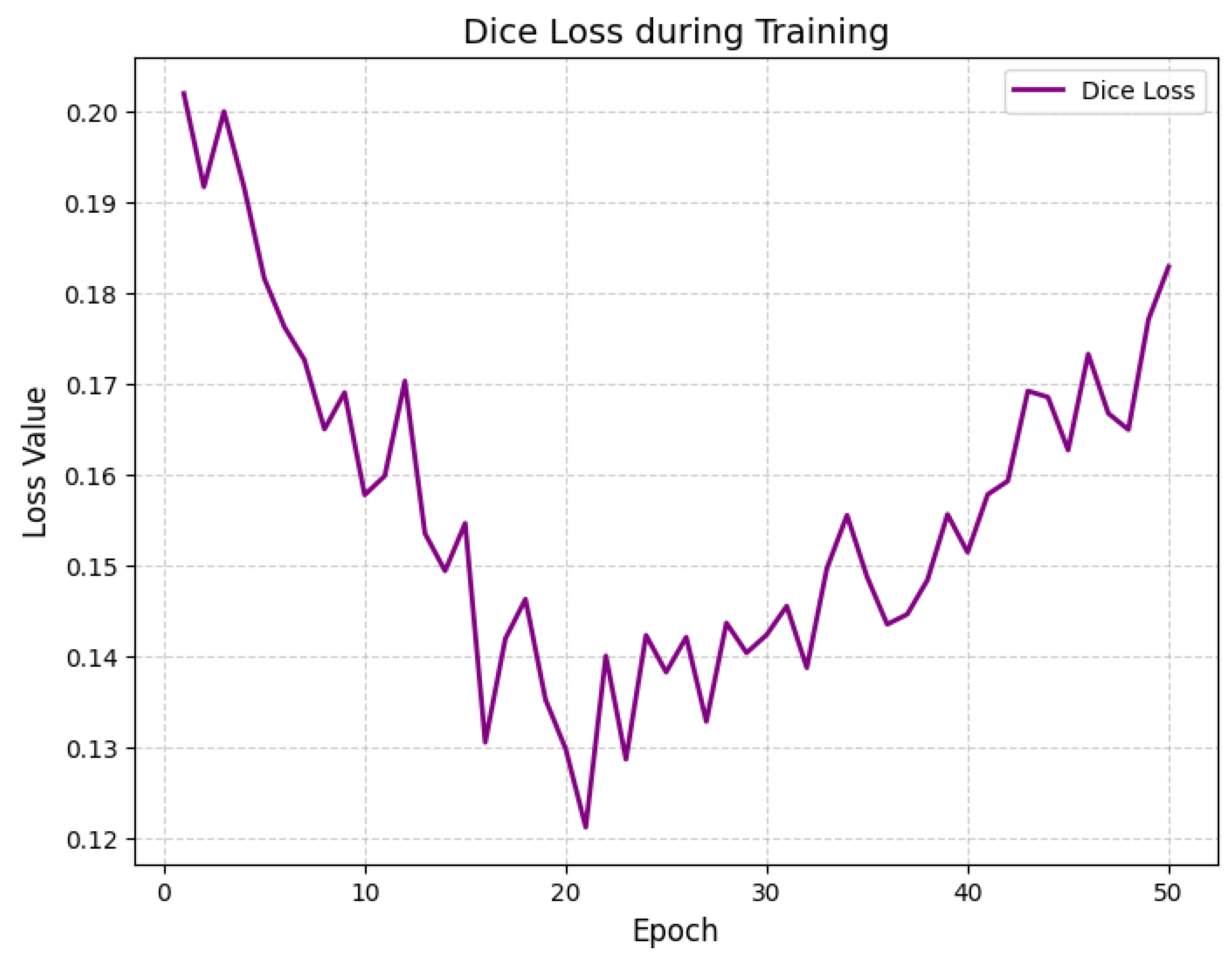
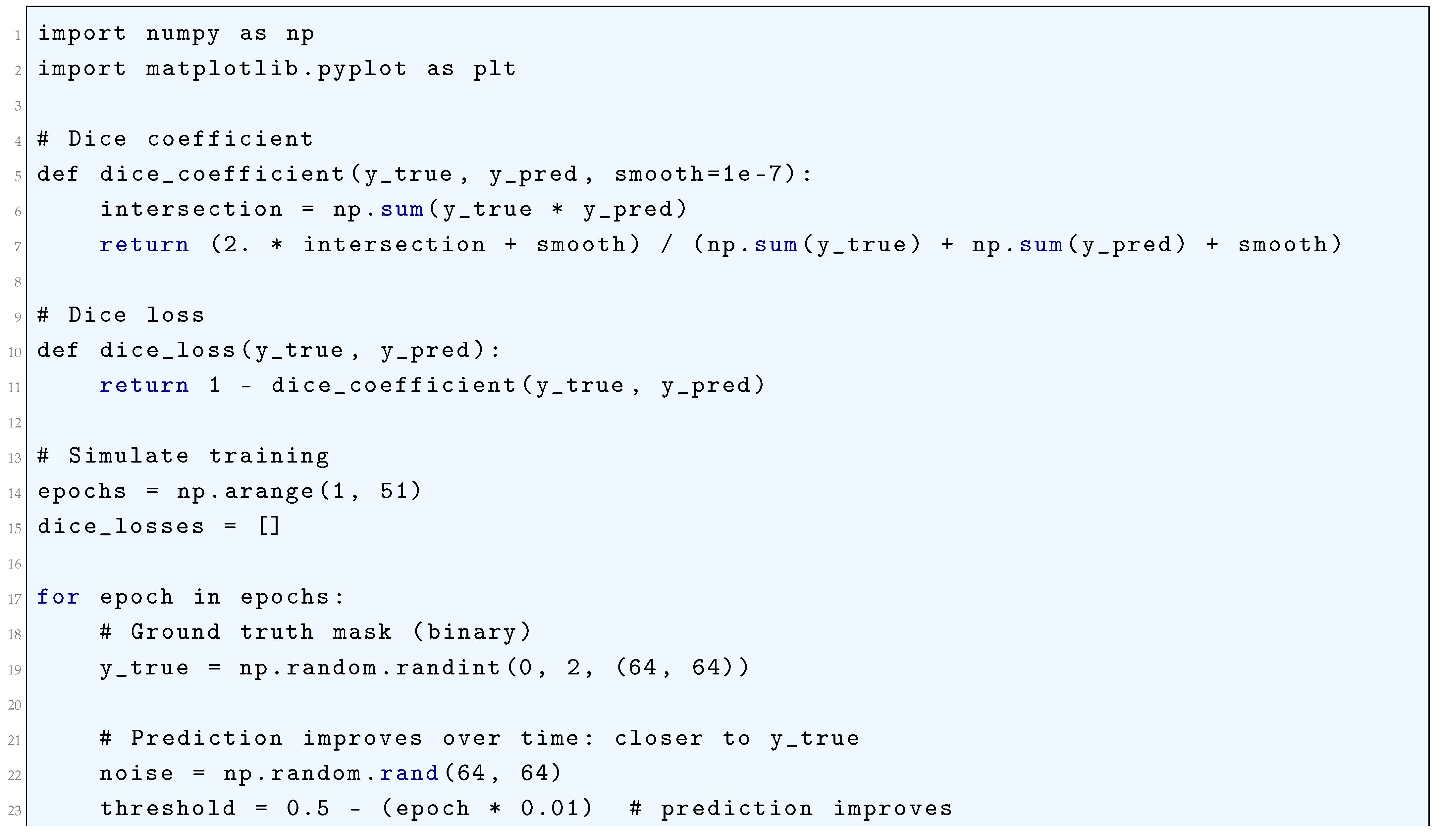
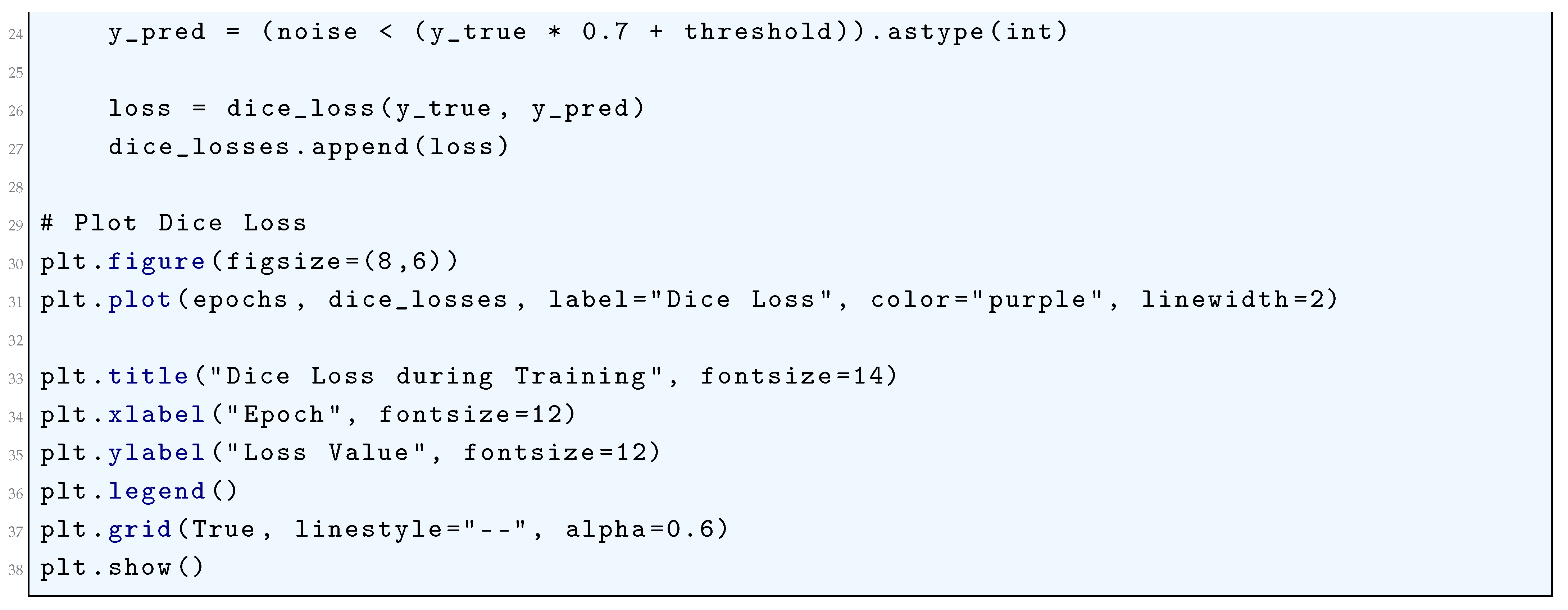
10.5.3.36 Python Code to Generate Figure 103 Illustrating Focal Loss vs Predicted Probability
The Python code below produces the Figure 103 illustrating Focal Loss vs Predicted Probability.
Figure 103.
Focal Loss vs Predicted Probability
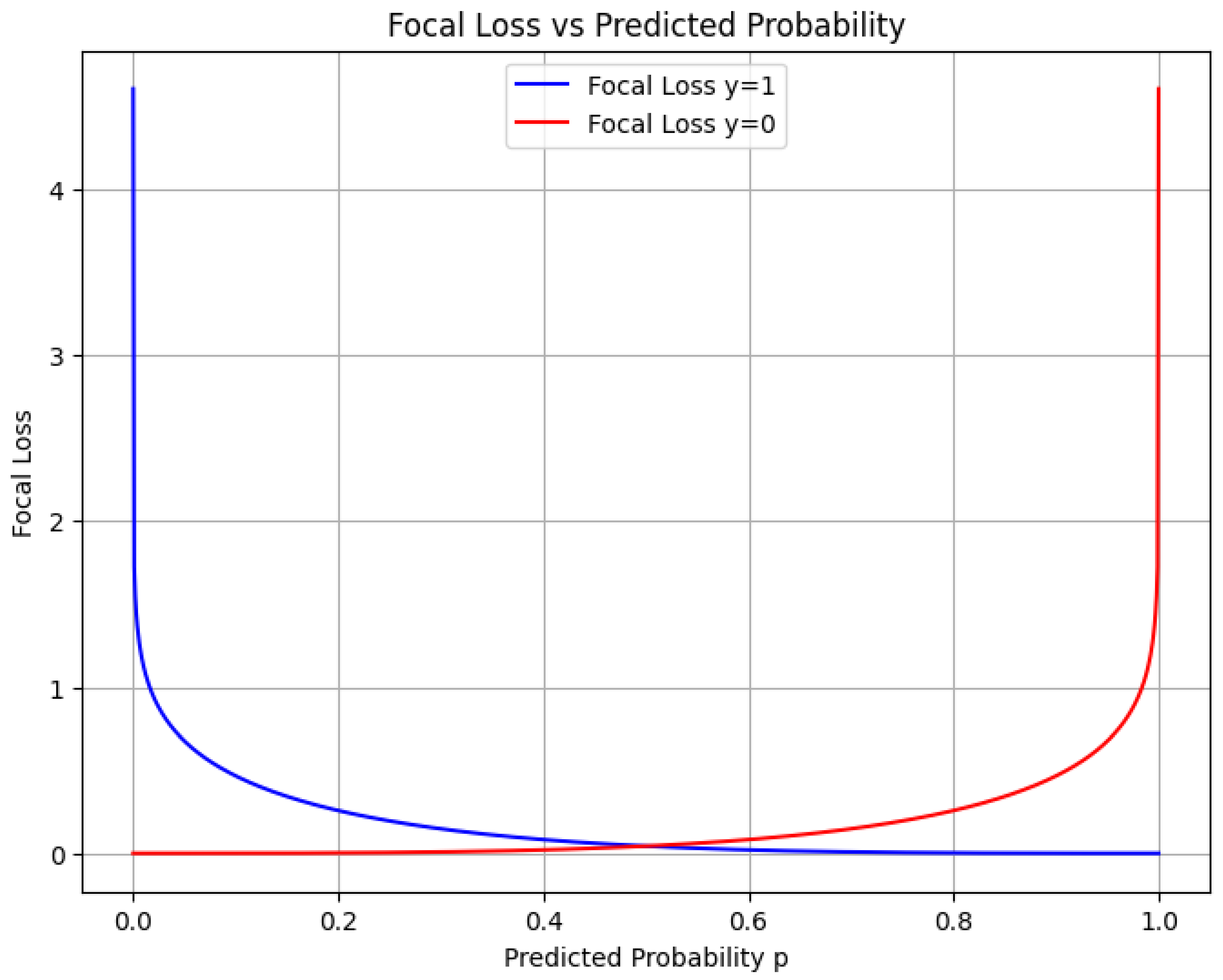
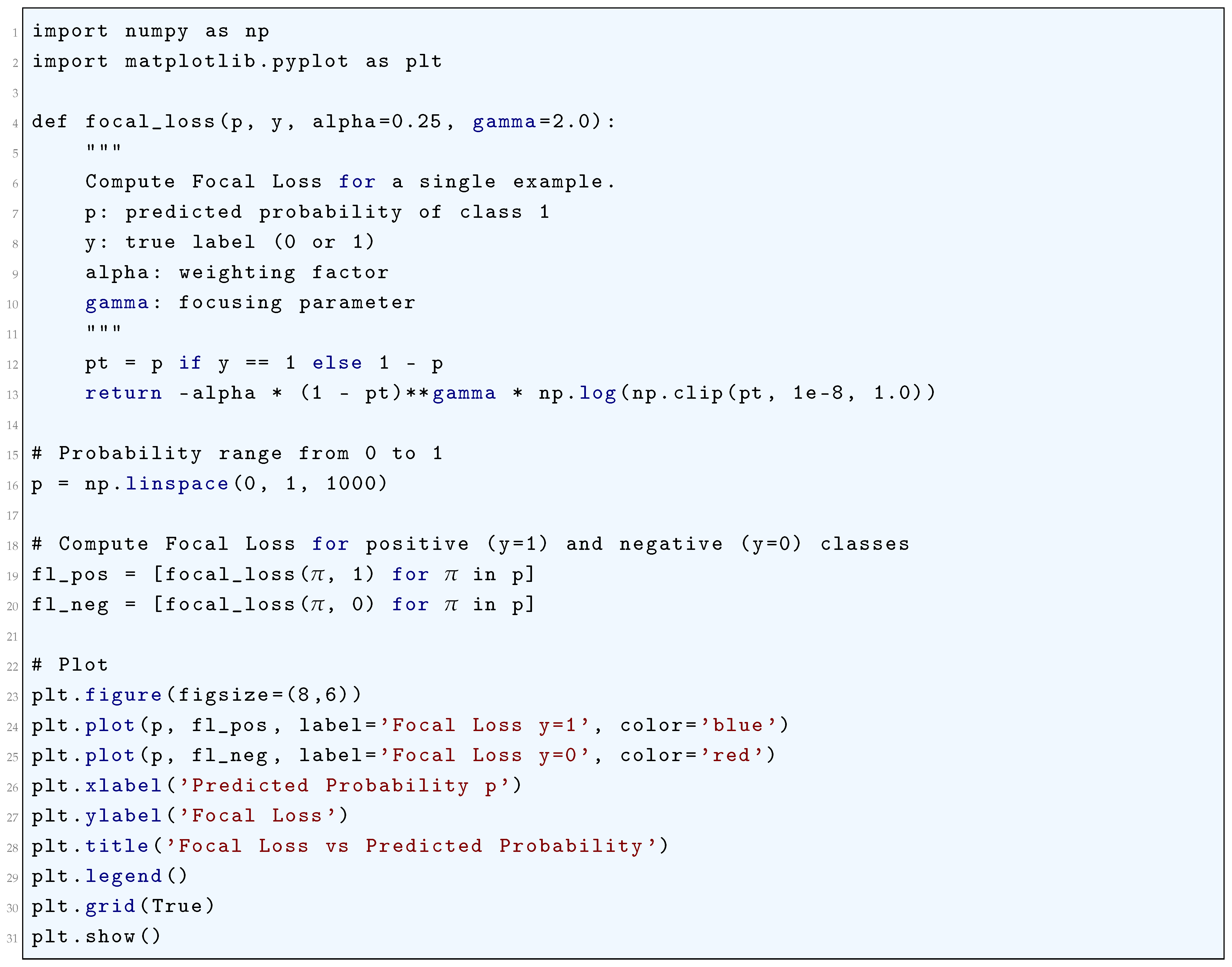
10.5.3.37 Python Code to Generate Figure 104 Illustrating Focal Loss vs Standard Binary Cross-Entropy
The Python code below produces the Figure 104 illustrating Focal Loss vs Standard Binary Cross-Entropy.
Figure 104.
Focal Loss vs Standard Binary Cross-Entropy
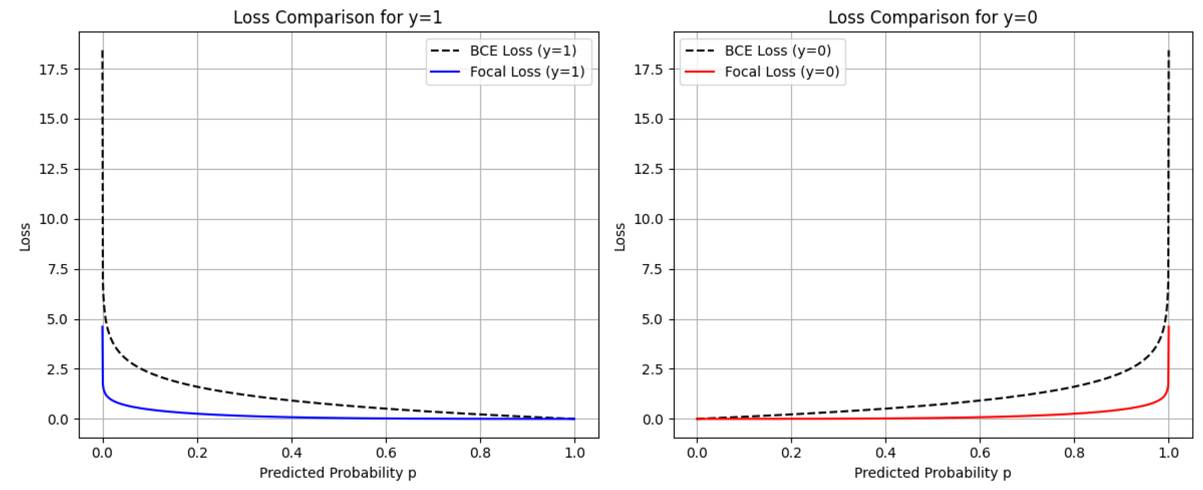
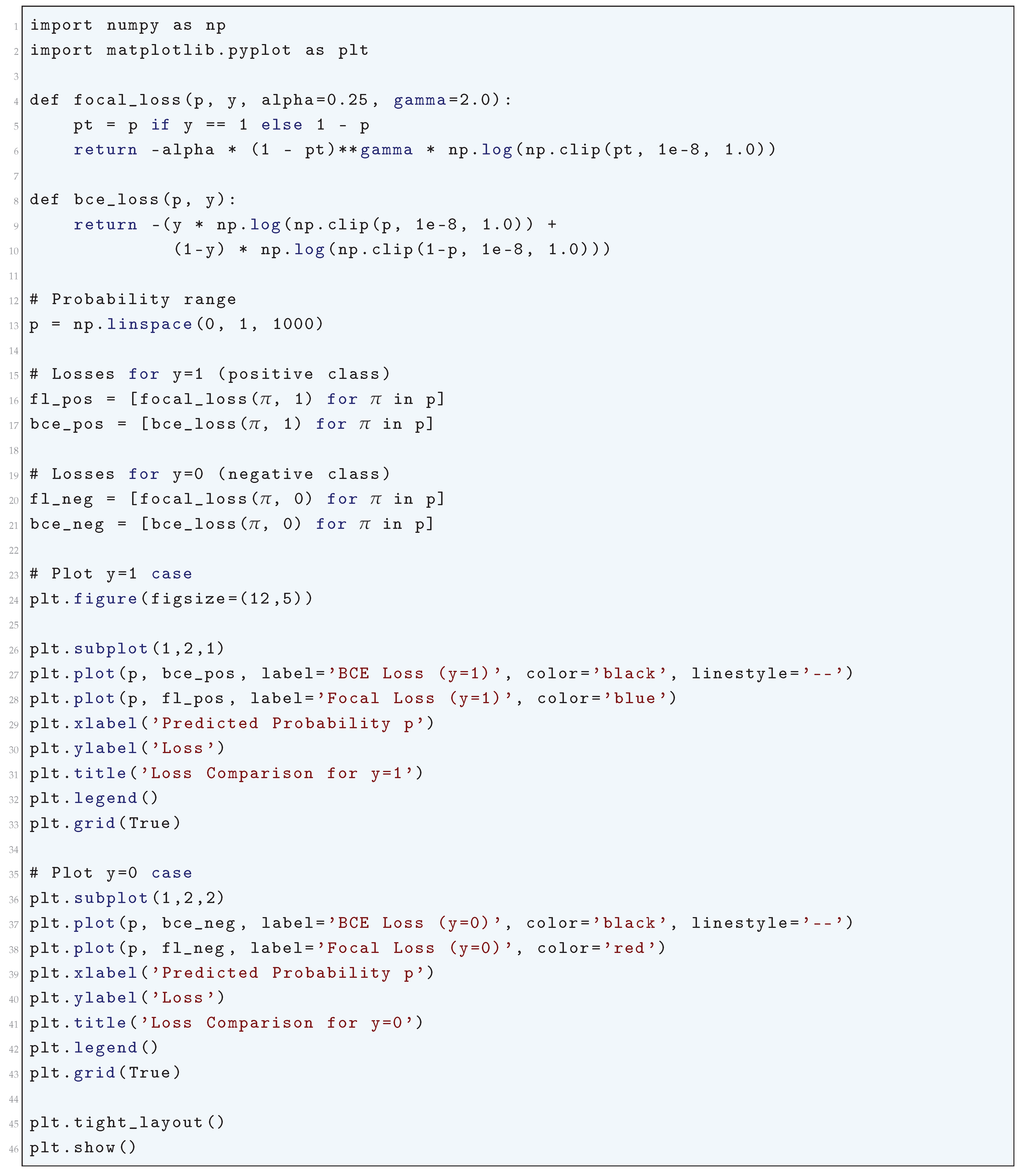
10.5.3.38 Python Code to Generate Figure 105 Illustrating Hinge Loss vs Prediction Score
The Python code below produces the Figure 105 illustrating Hinge Loss vs Prediction Score.
Figure 105.
Hinge Loss vs Prediction Score
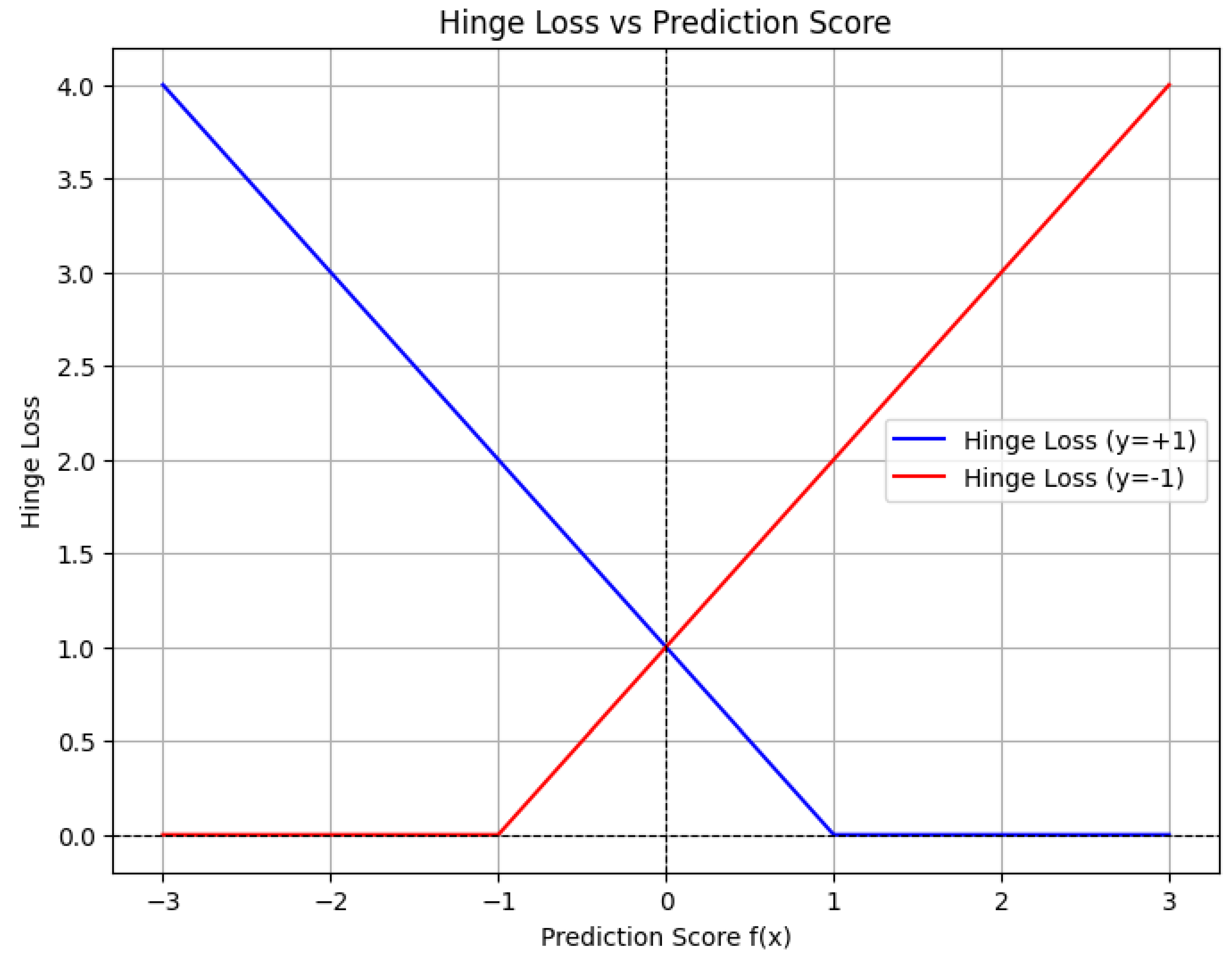
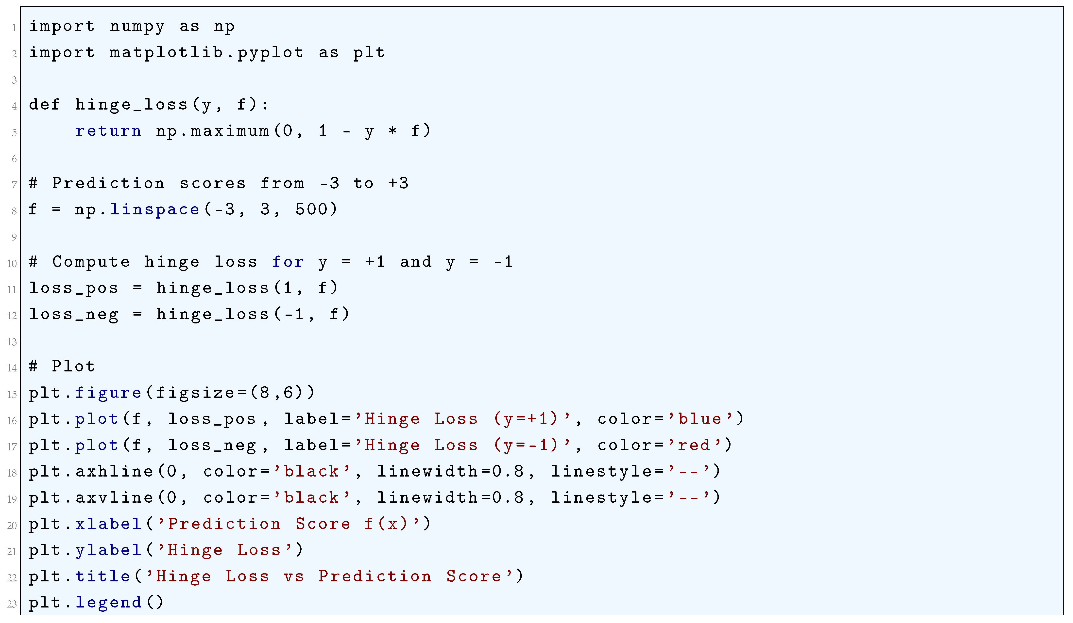

10.5.3.39 Python Code to Generate Figure 106 Illustrating Comparison of the Standard Hinge Loss and the Squared Hinge Loss
The Python code below produces the Figure 106 illustrating Comparison of the Standard Hinge Loss and the Squared Hinge Loss.
Figure 106.
Comparison of the Standard Hinge Loss and the Squared Hinge Loss
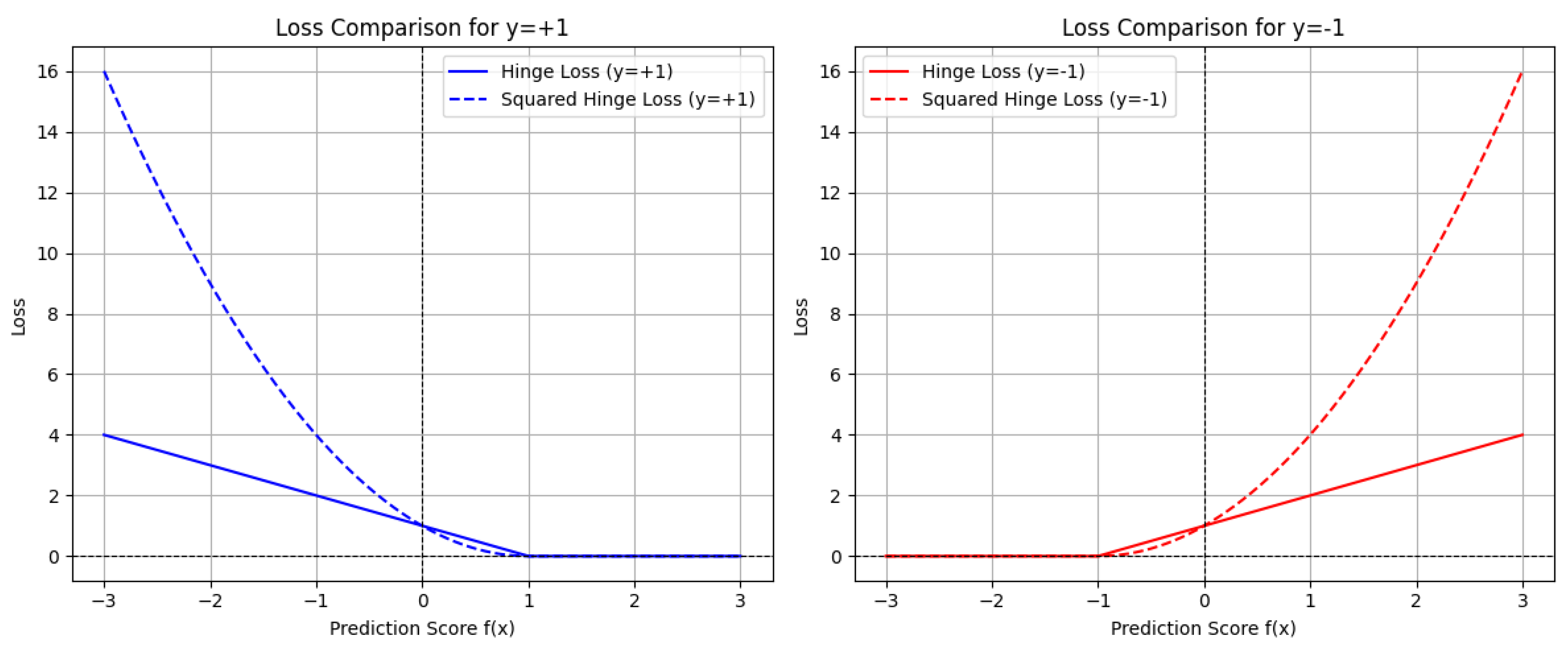
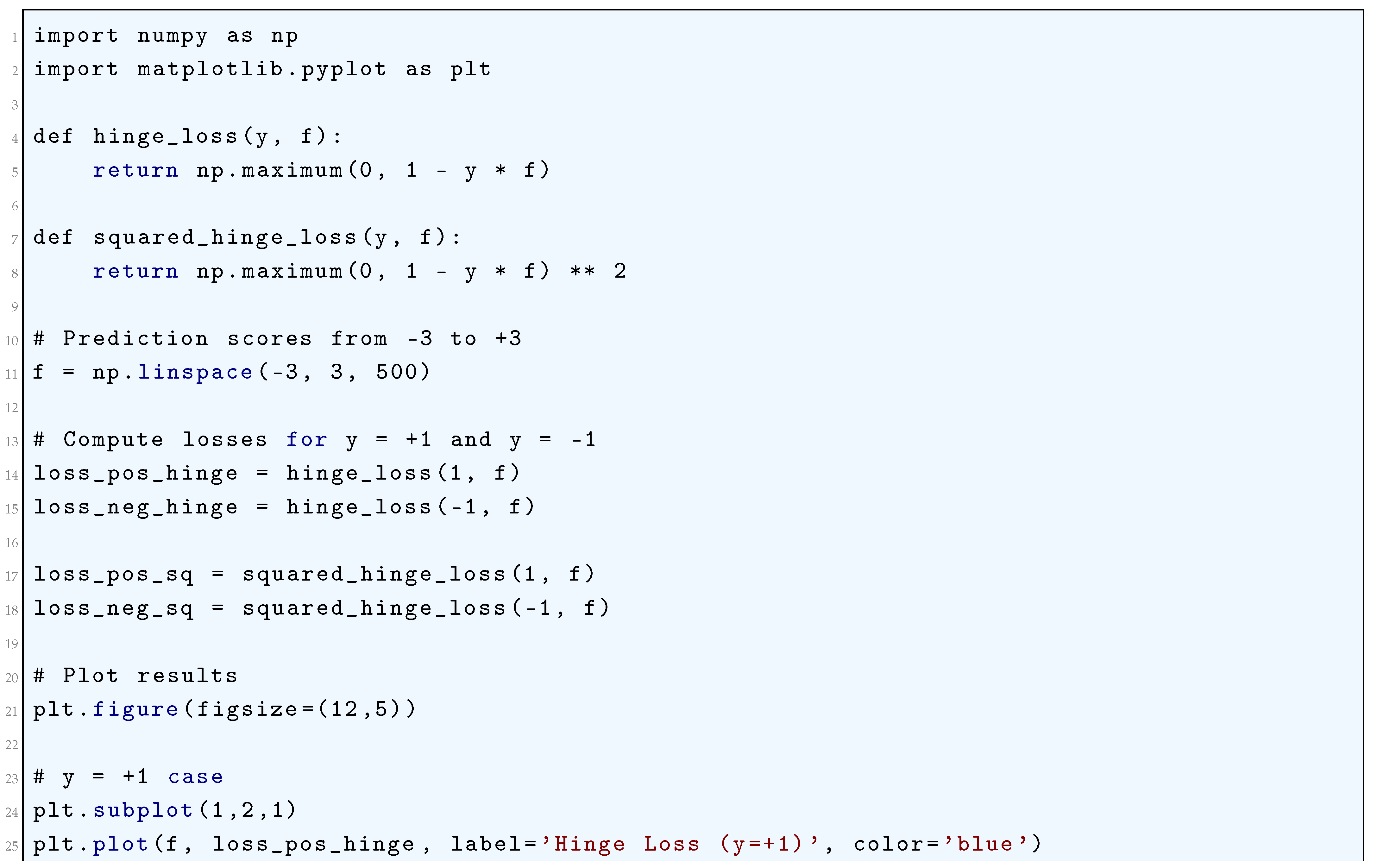
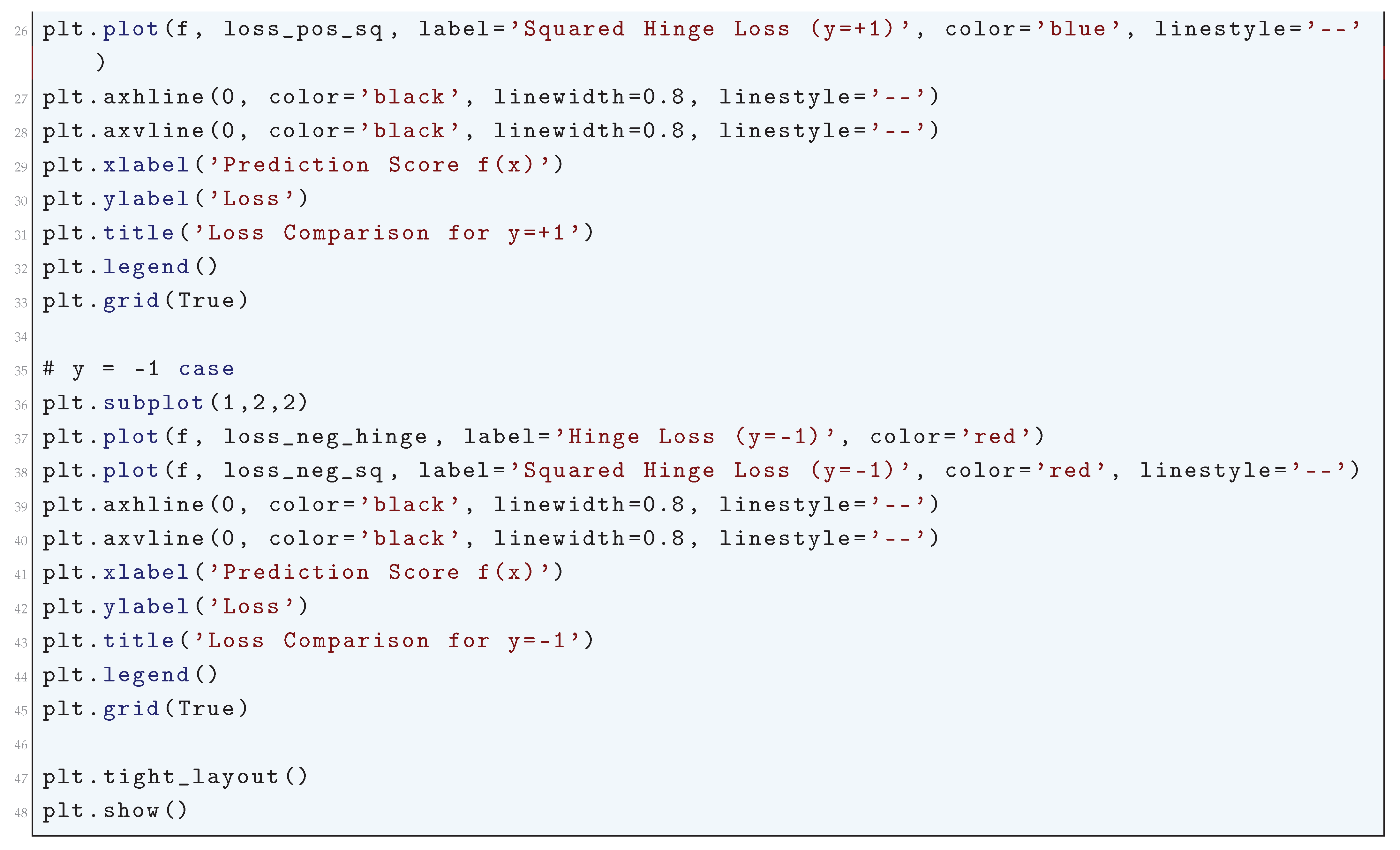
10.5.3.40 Python Code to Generate Figure 107 Illustrating Value Loss (MSE) for Different Targets
The Python code below produces the Figure 107 illustrating Value Loss (MSE) for Different Targets.
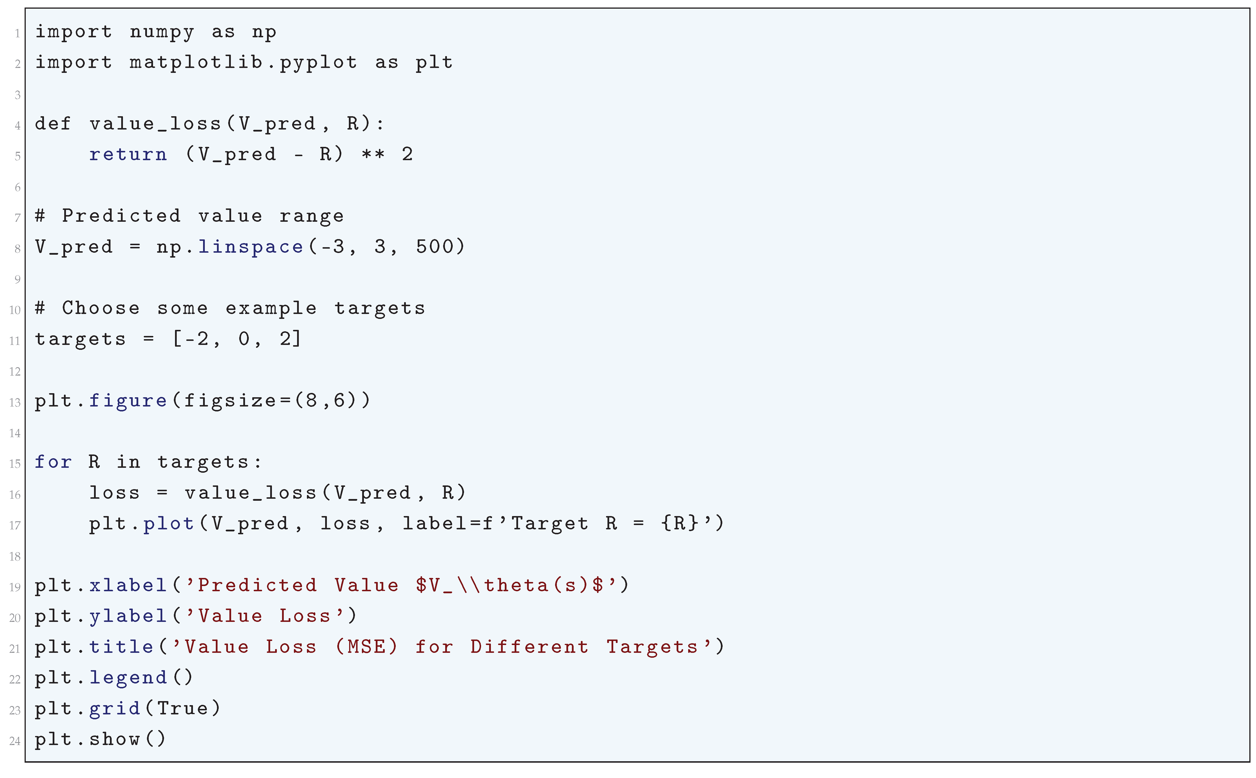
Figure 107.
Value Loss (MSE) for Different Targets
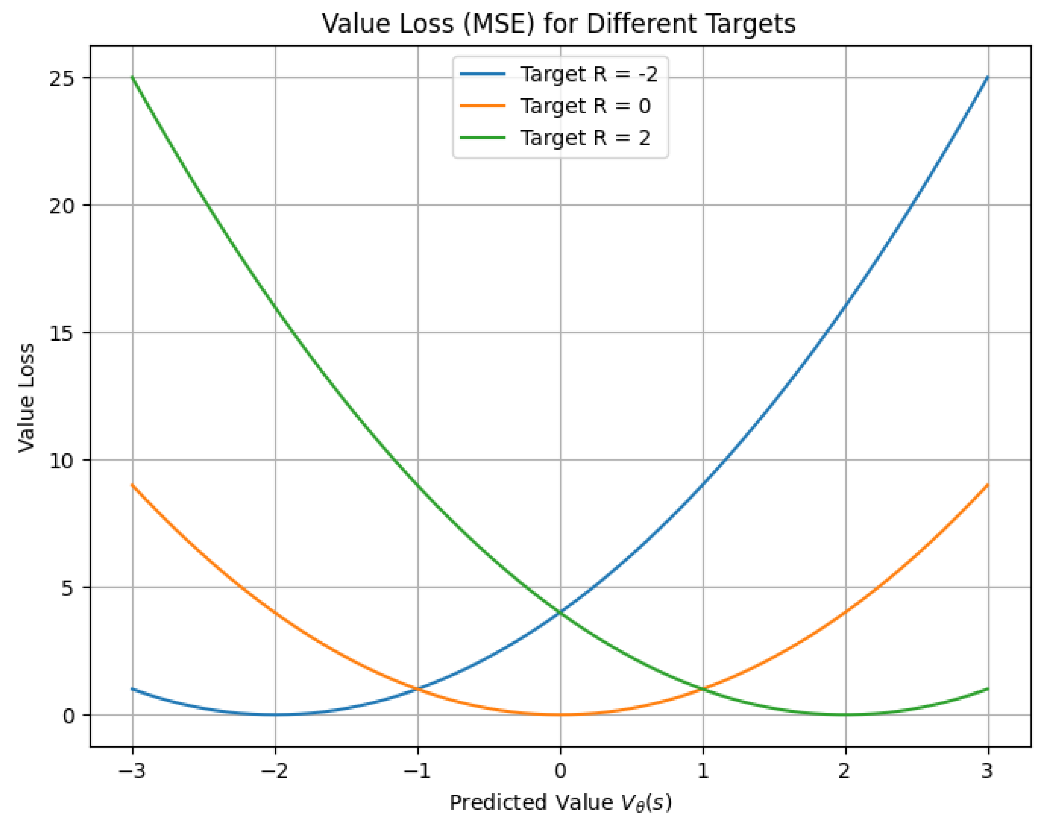
10.5.3.41 Python Code to Generate Figure 108 Illustrating Value Loss (MSE) vs Huber Loss
The Python code below produces the Figure 108 illustrating Value Loss (MSE) vs Huber Loss.
Figure 108.
Value Loss (MSE) vs Huber Loss
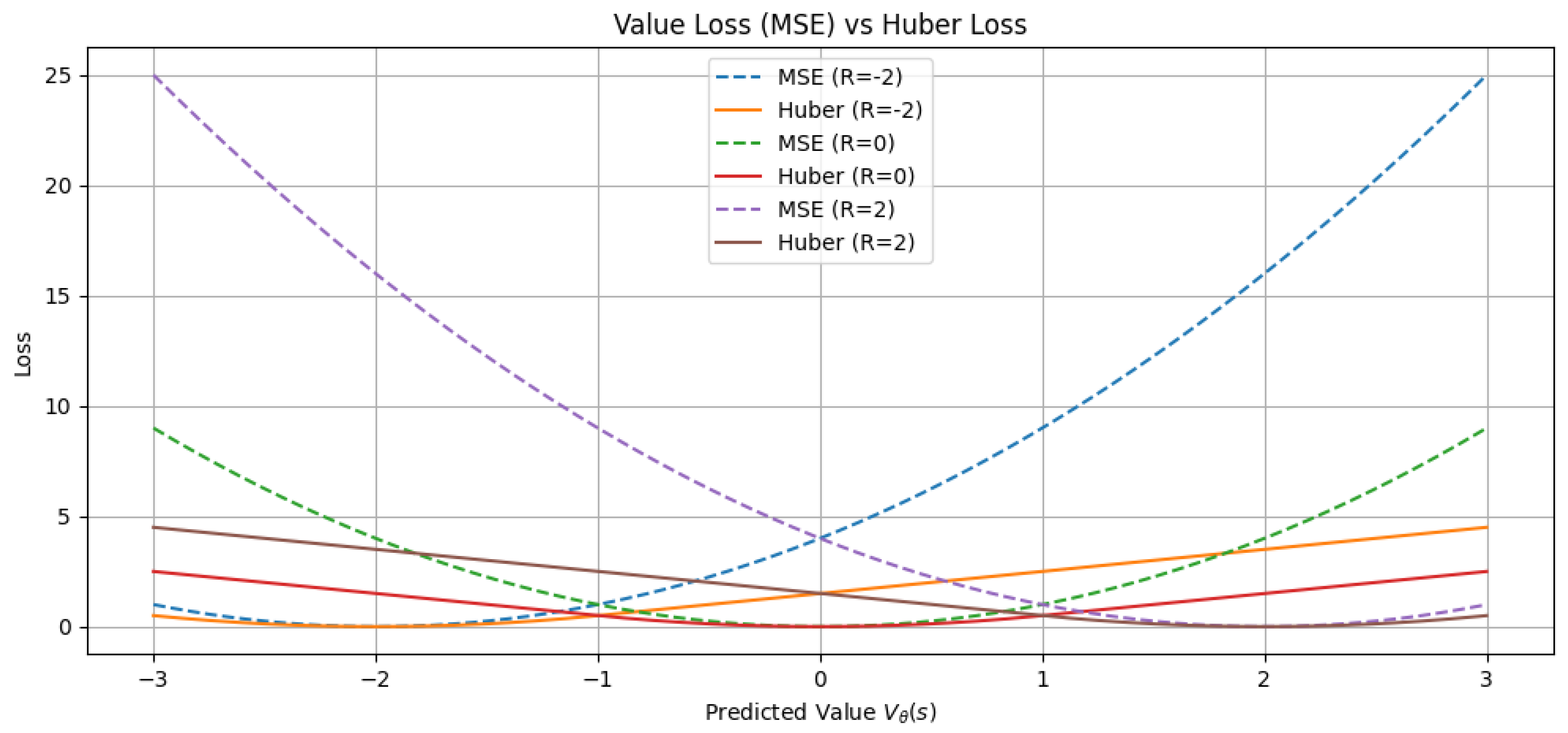

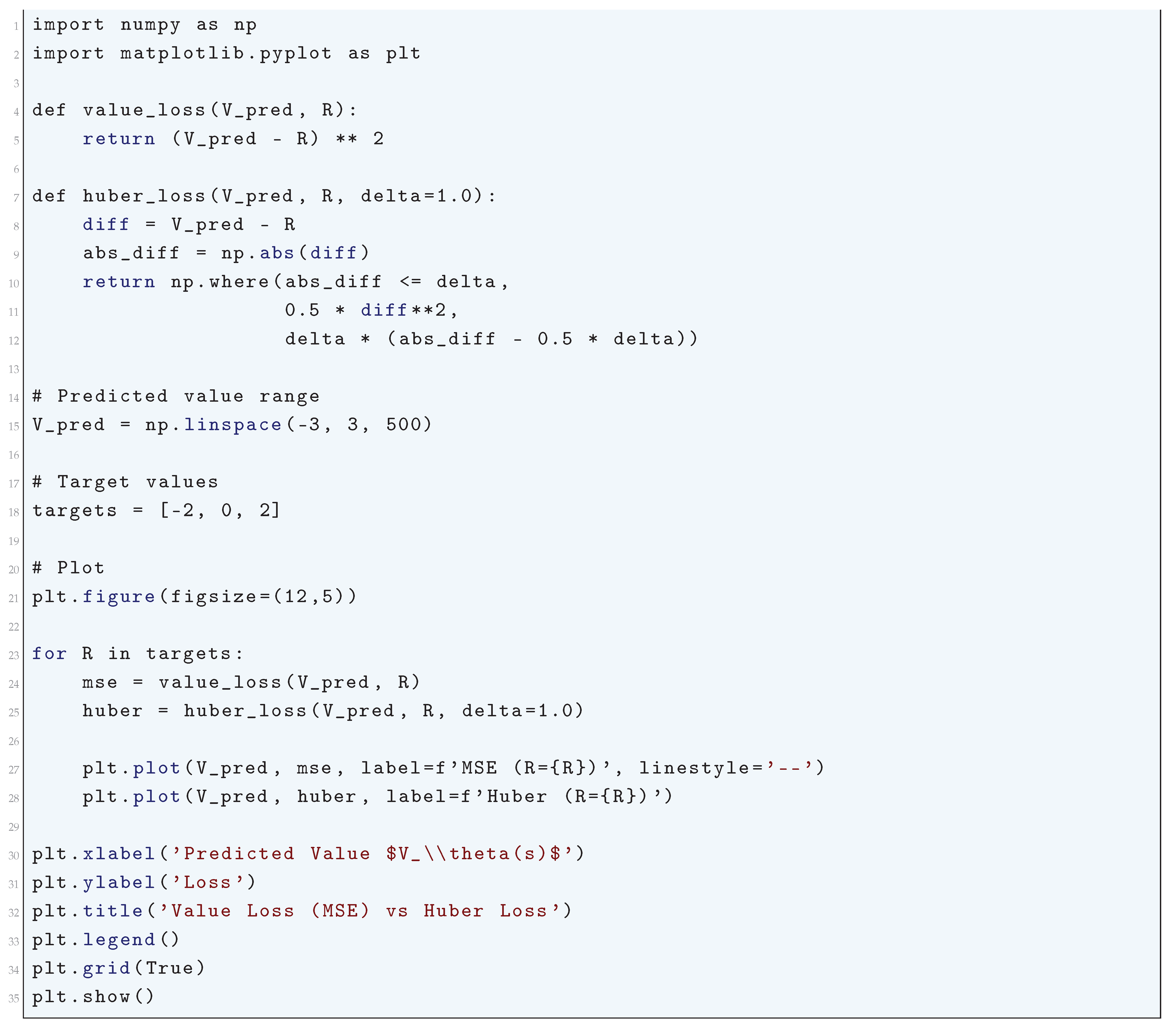
10.5.3.42 Python Code to Generate Figure 109 Illustrating Policy Loss vs Action Probability
The Python code below produces the Figure 109 illustrating Policy Loss vs Action Probability.
Figure 109.
Policy Loss vs Action Probability
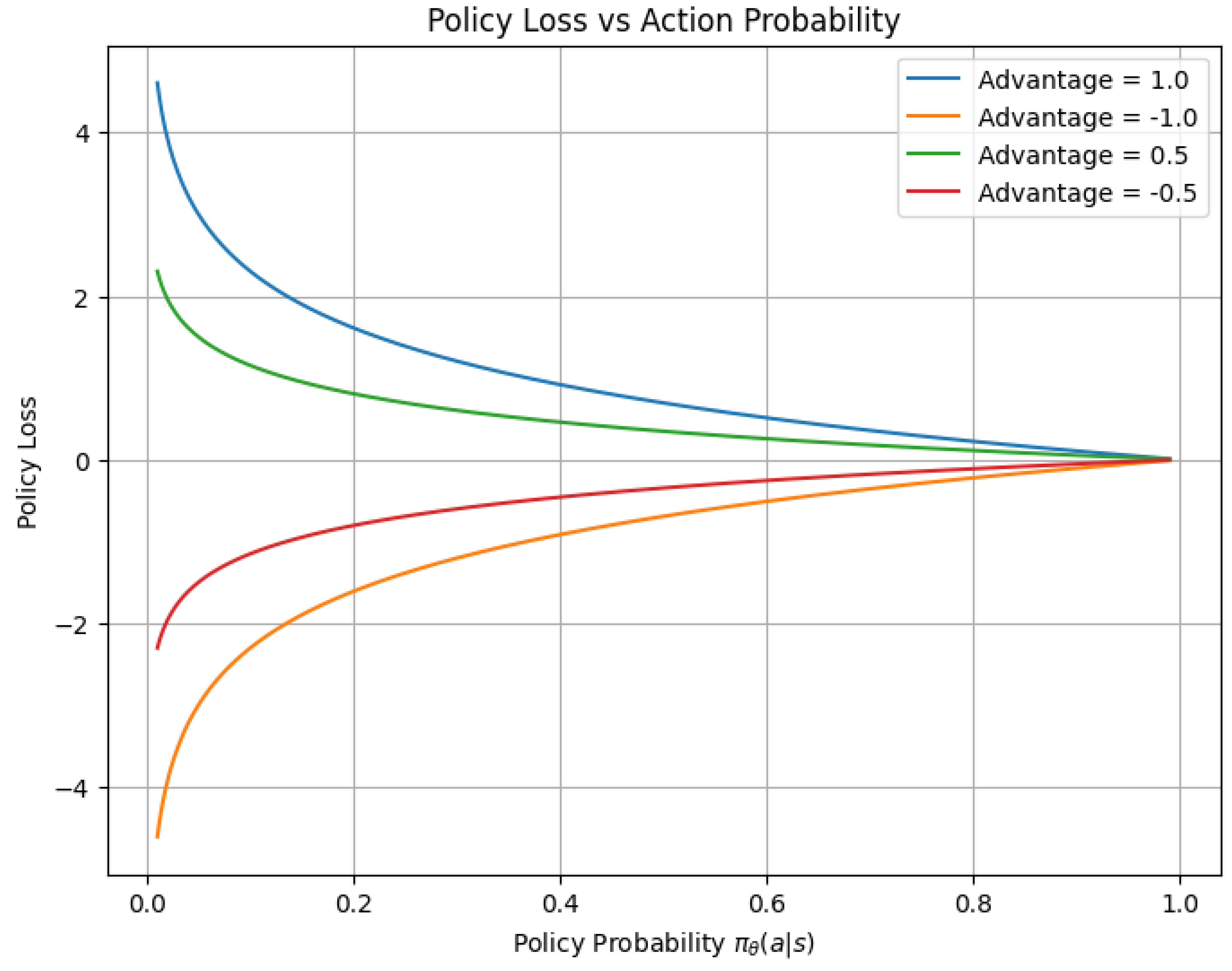
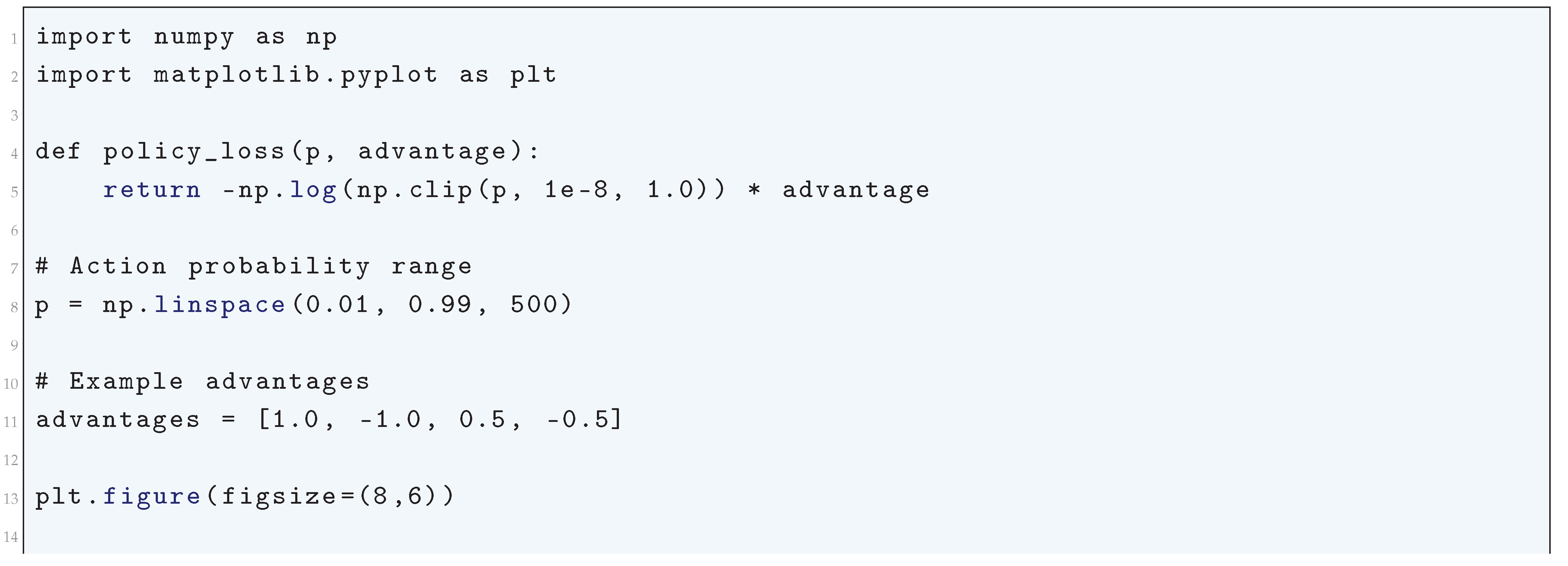
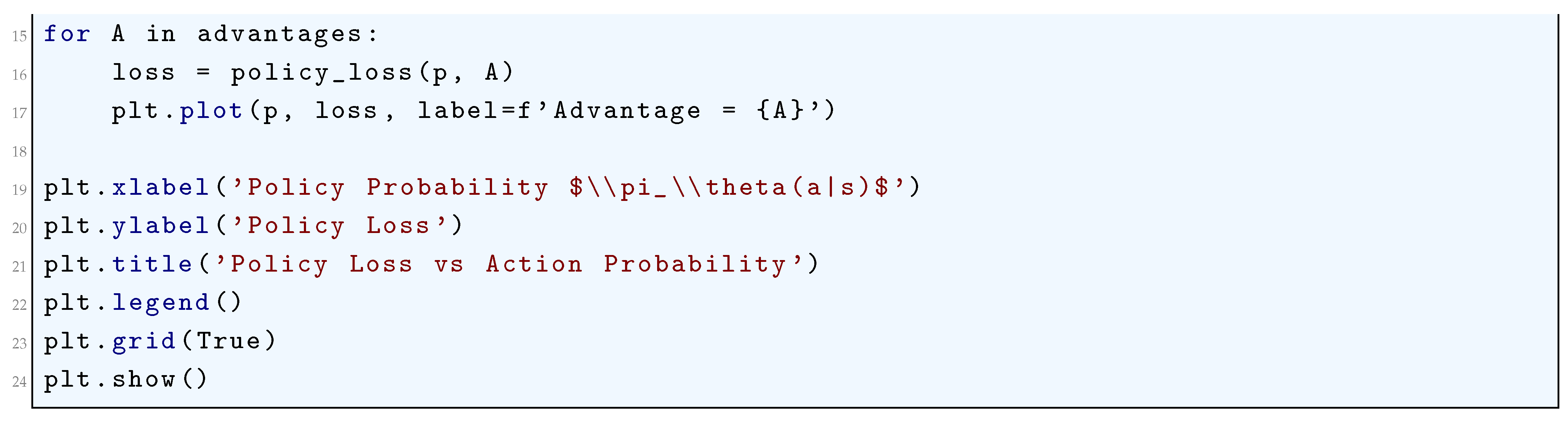
10.5.3.43 Python Code to Generate Figure 110 Illustrating PPO Clipped Surrogate Objective
The Python code below produces the Figure 110 illustrating PPO Clipped Surrogate Objective.
Figure 110.
PPO Clipped Surrogate Objective
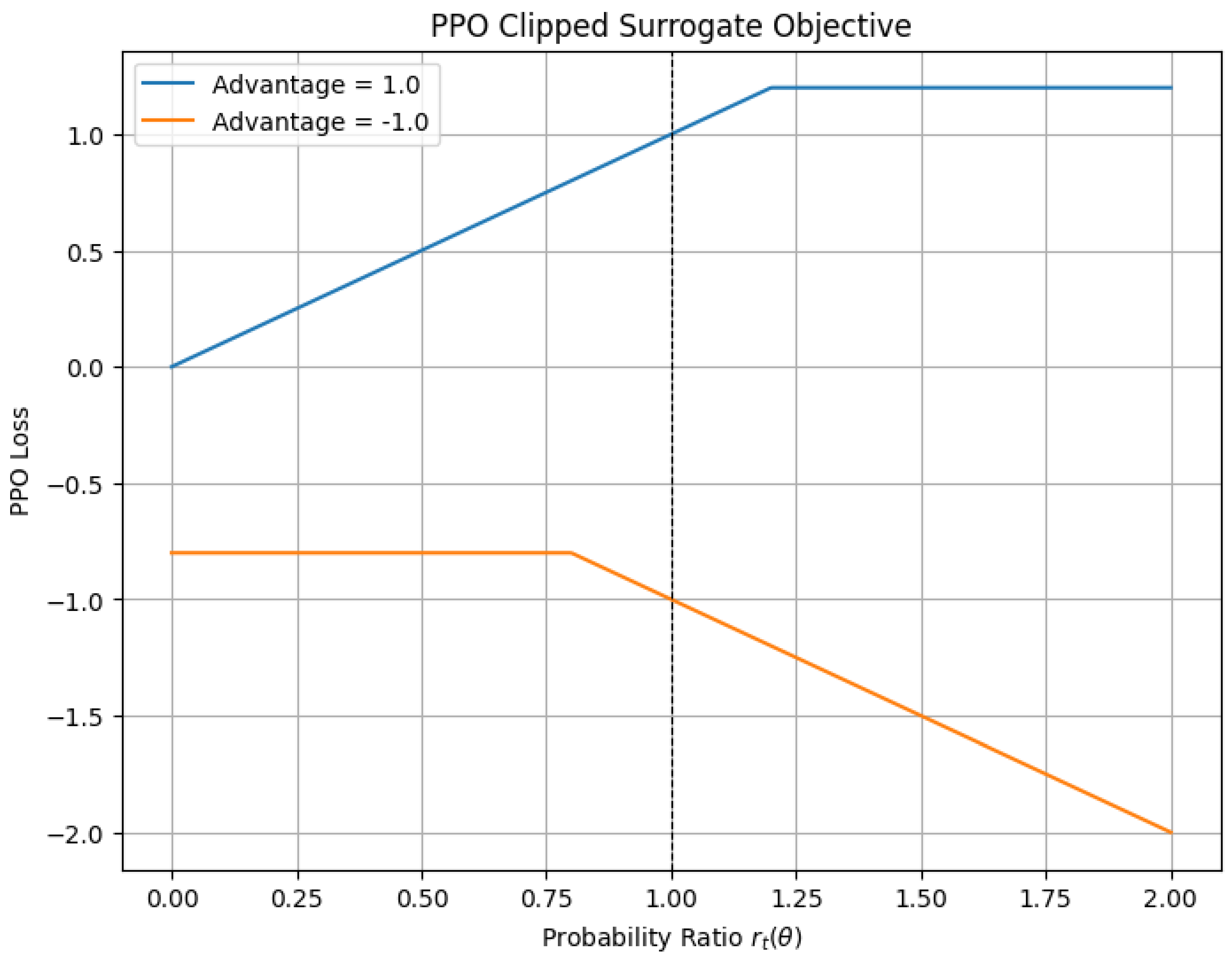
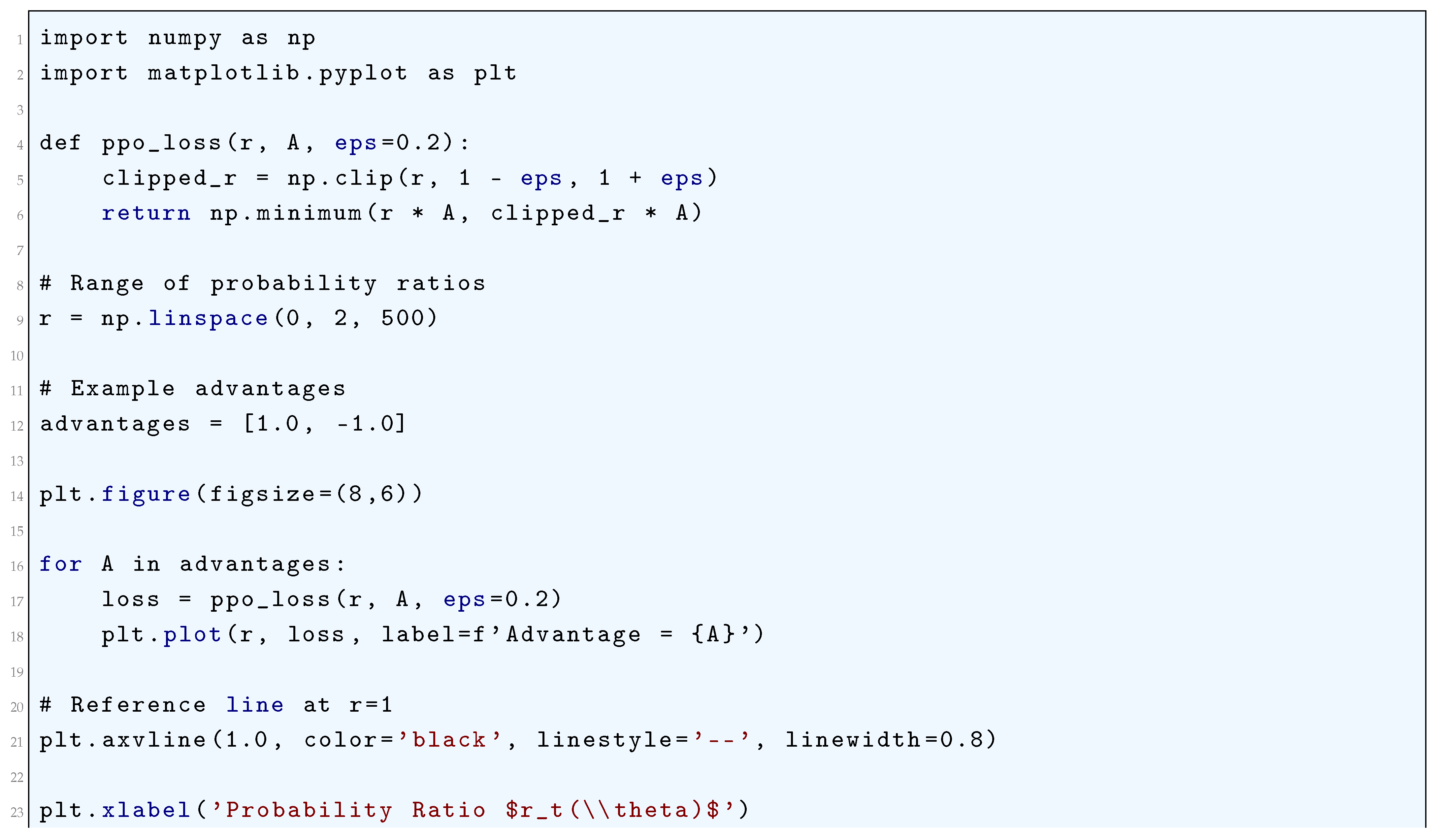
10.5.3.44 Python Code to Generate Figure 111 Illustrating PPO Loss Comparison
The Python code below produces the Figure 111 illustrating PPO Loss Comparison.
Figure 111.
PPO Loss Comparison
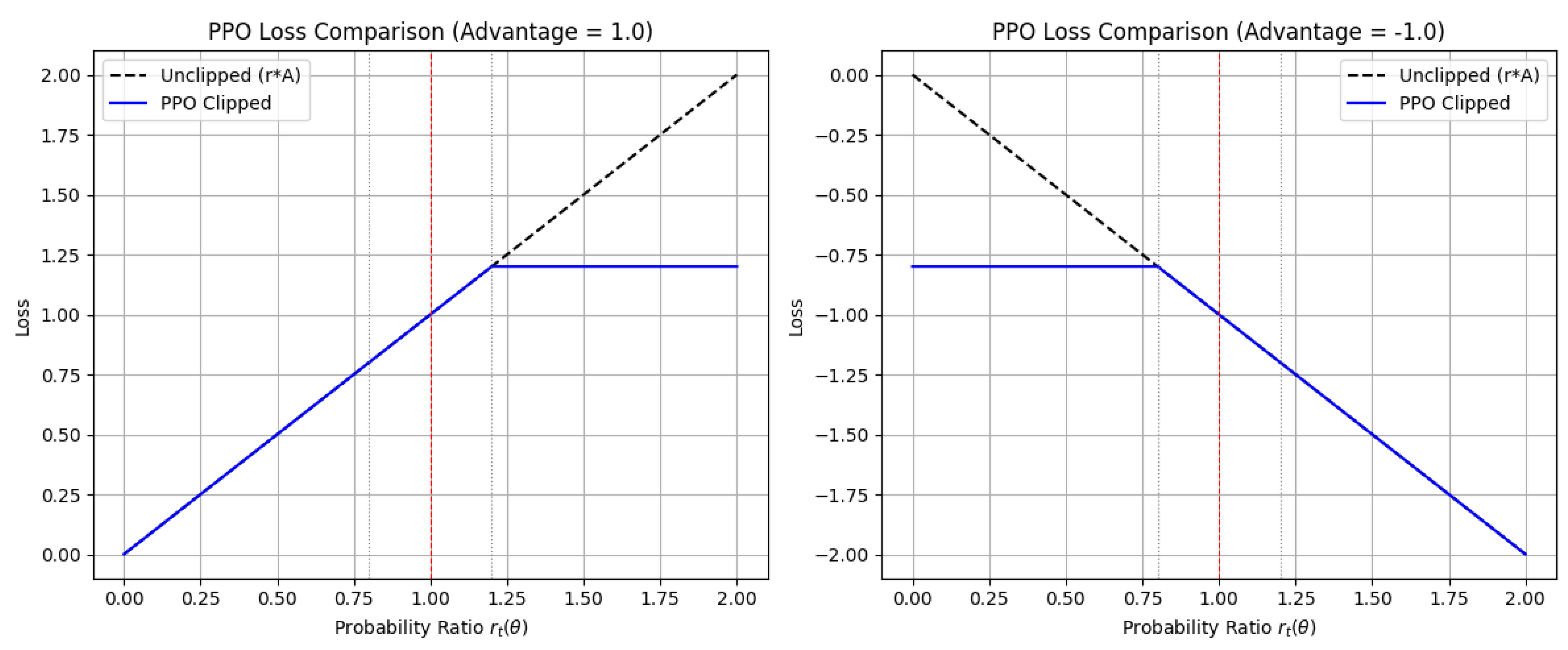
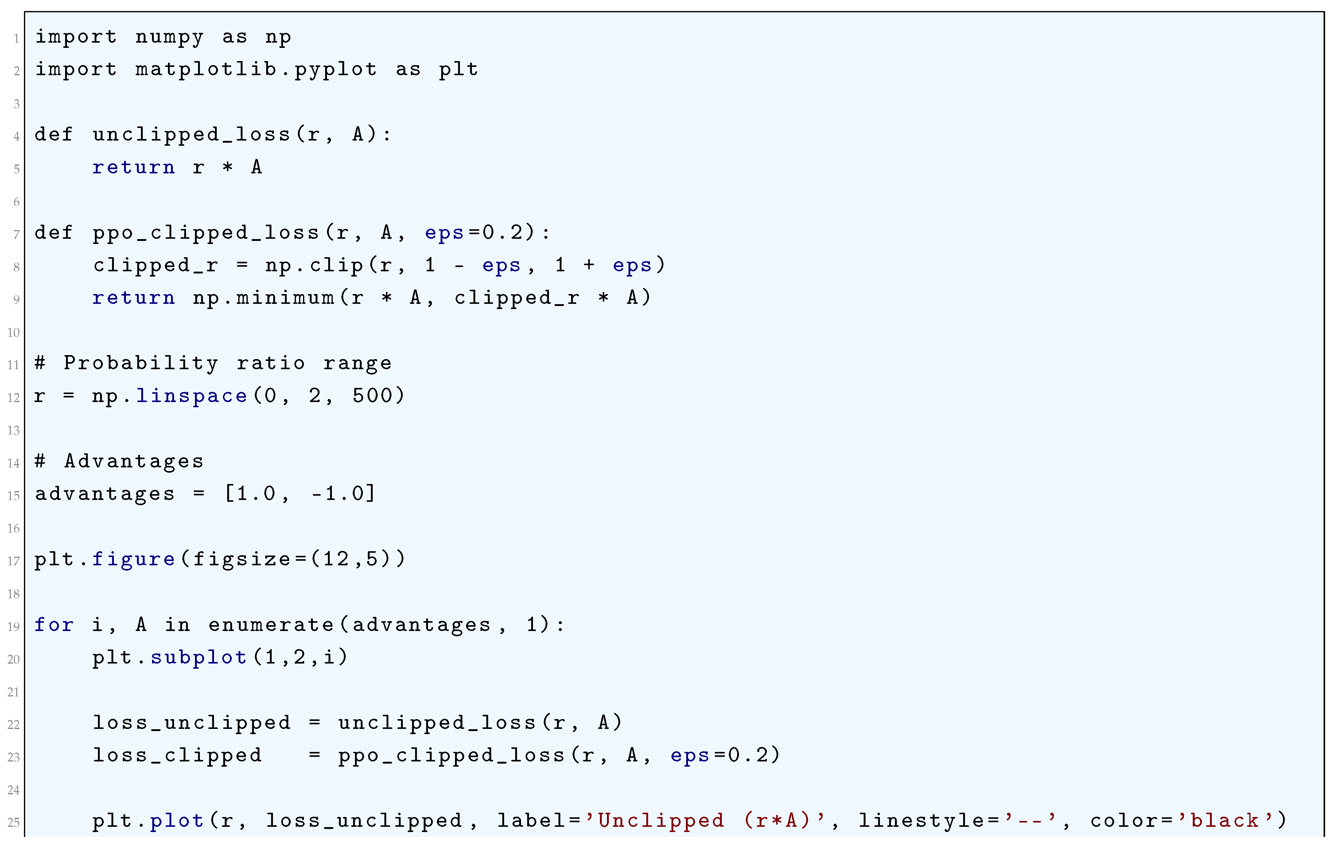
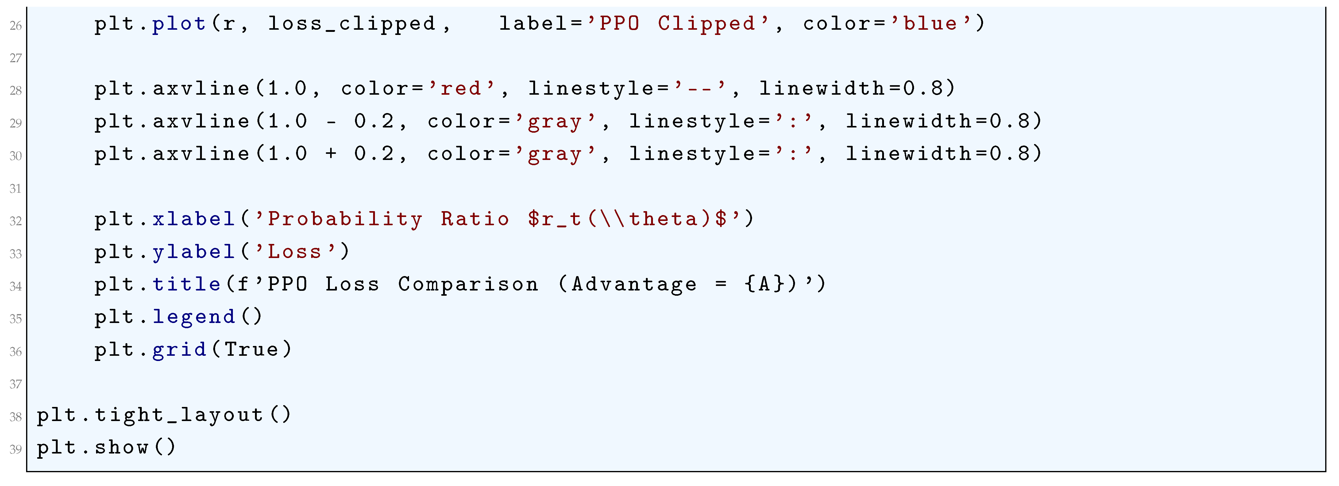
10.5.3.45 Python Code to Generate Figure 112 Illustrating PPO Clipped Surrogate Loss with Entropy Regularization
The Python code below produces the Figure 112 illustrating PPO Clipped Surrogate Loss with Entropy Regularization.
Figure 112.
PPO Clipped Surrogate Loss with Entropy Regularization
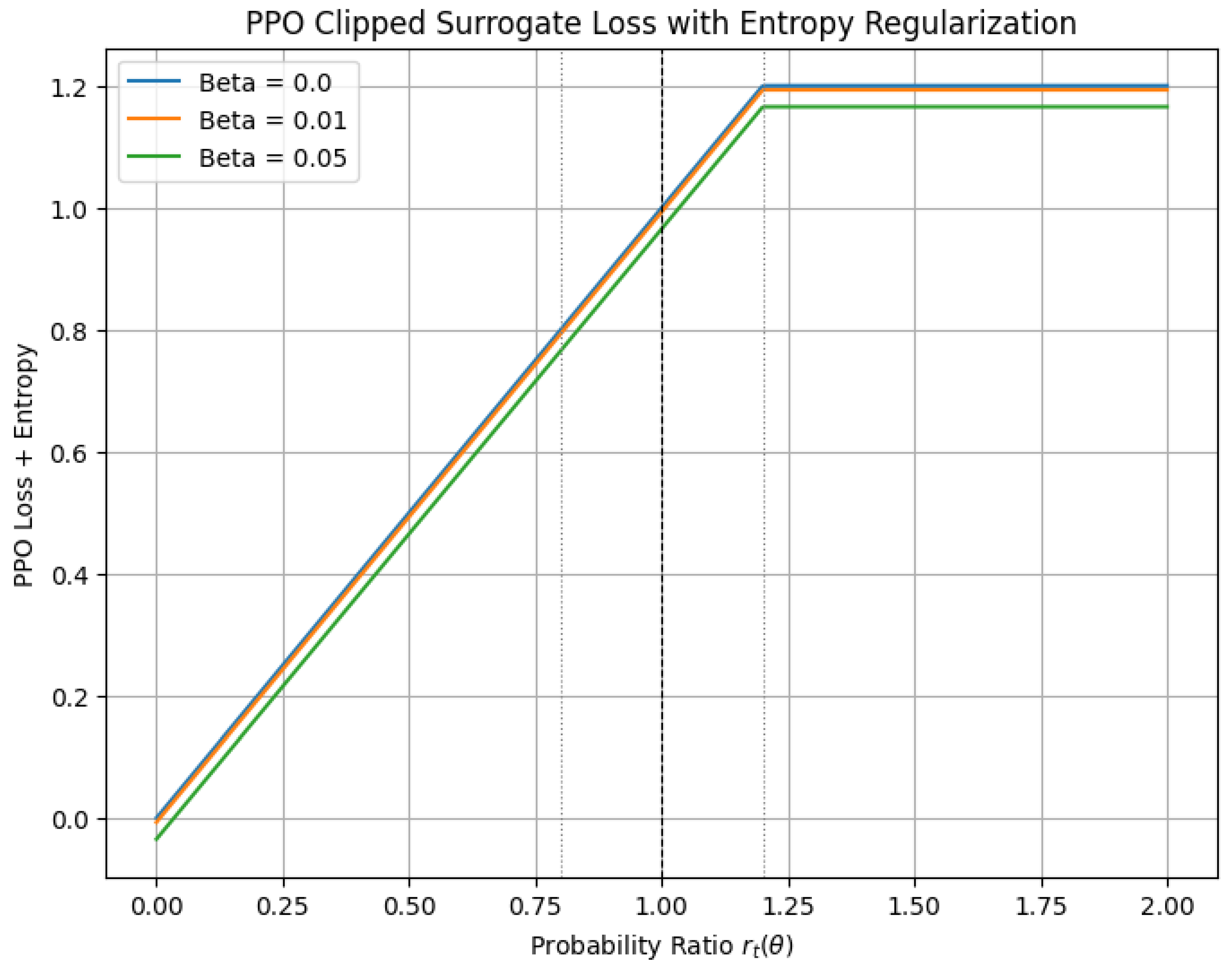
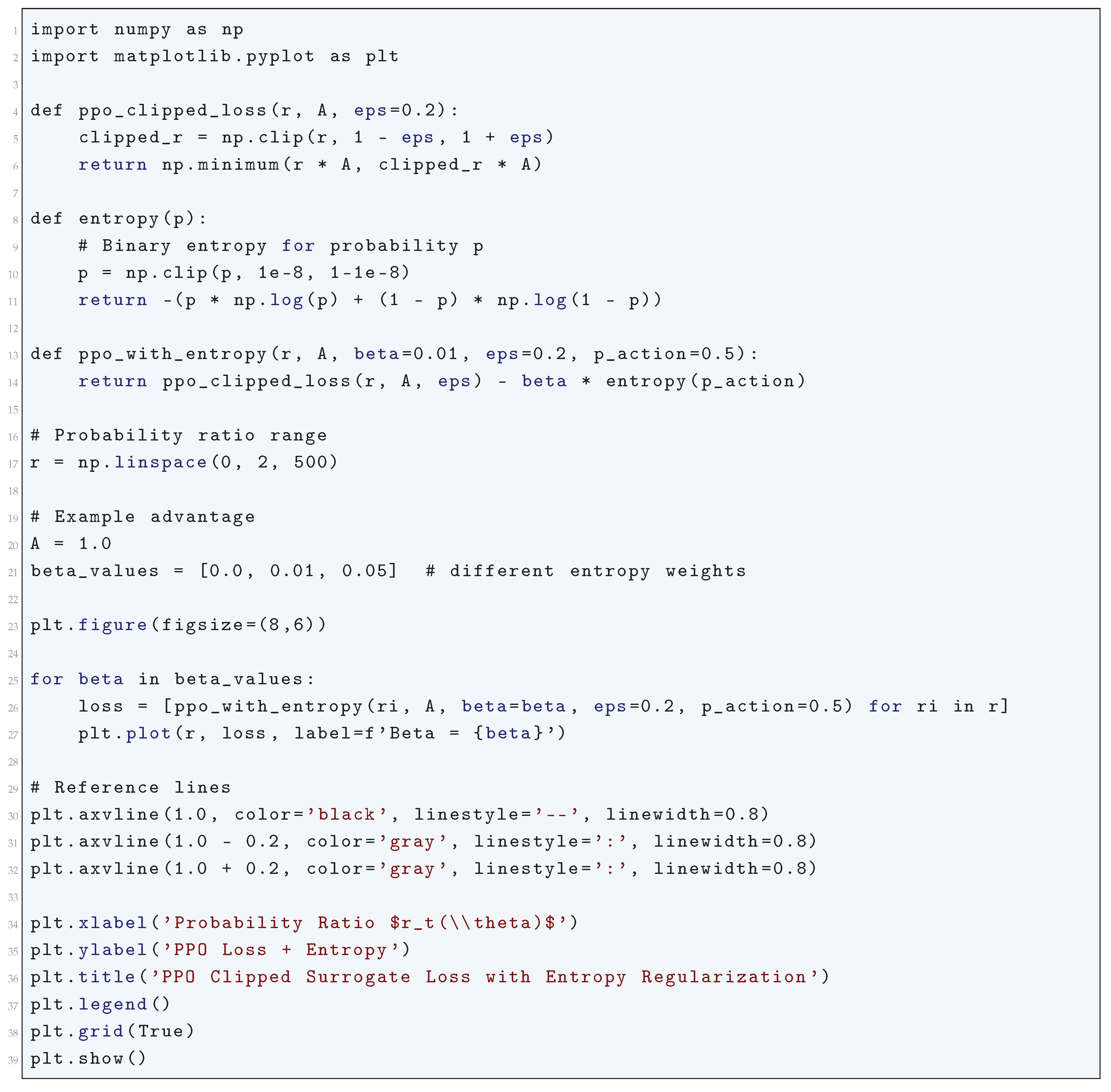
10.5.3.46 Python Code to Generate Figure 113 Comparing PPO Unclipped, PPO Clipped, PPO + Entropy
The Python code below produces the Figure 113 comparing PPO Unclipped, PPO Clipped, PPO + Entropy.
Figure 113.
Comparison: PPO Unclipped, PPO Clipped, PPO + Entropy
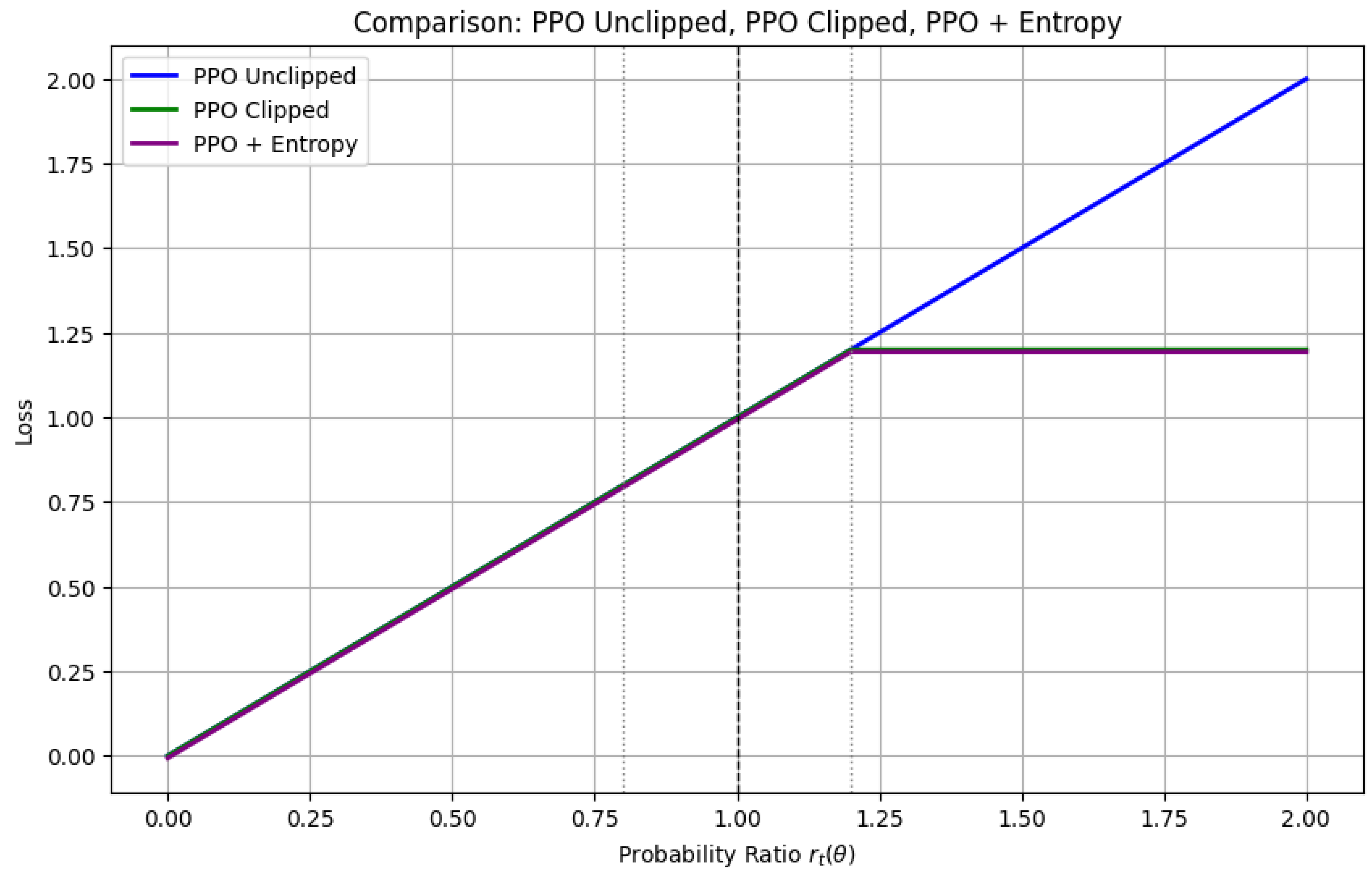
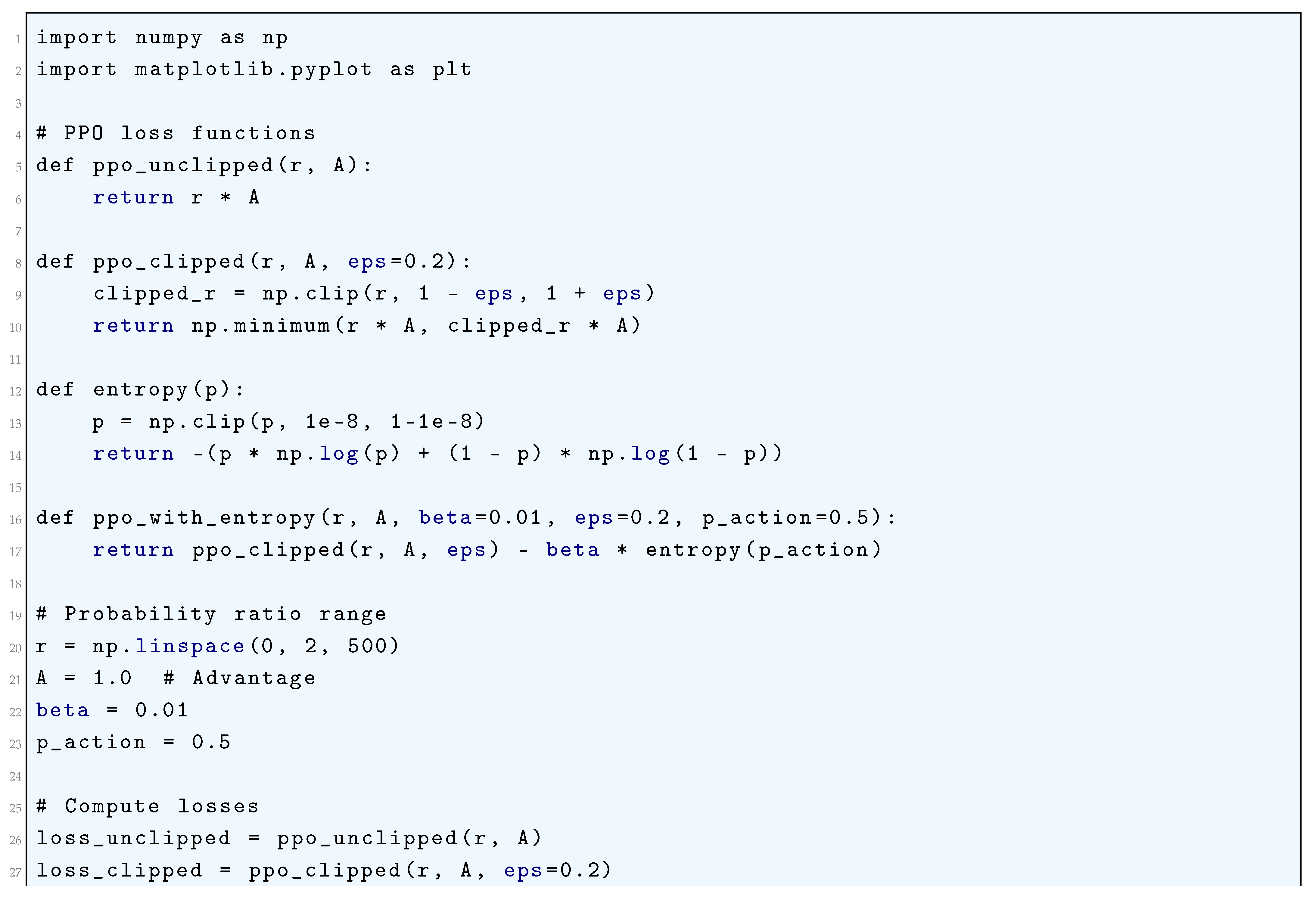
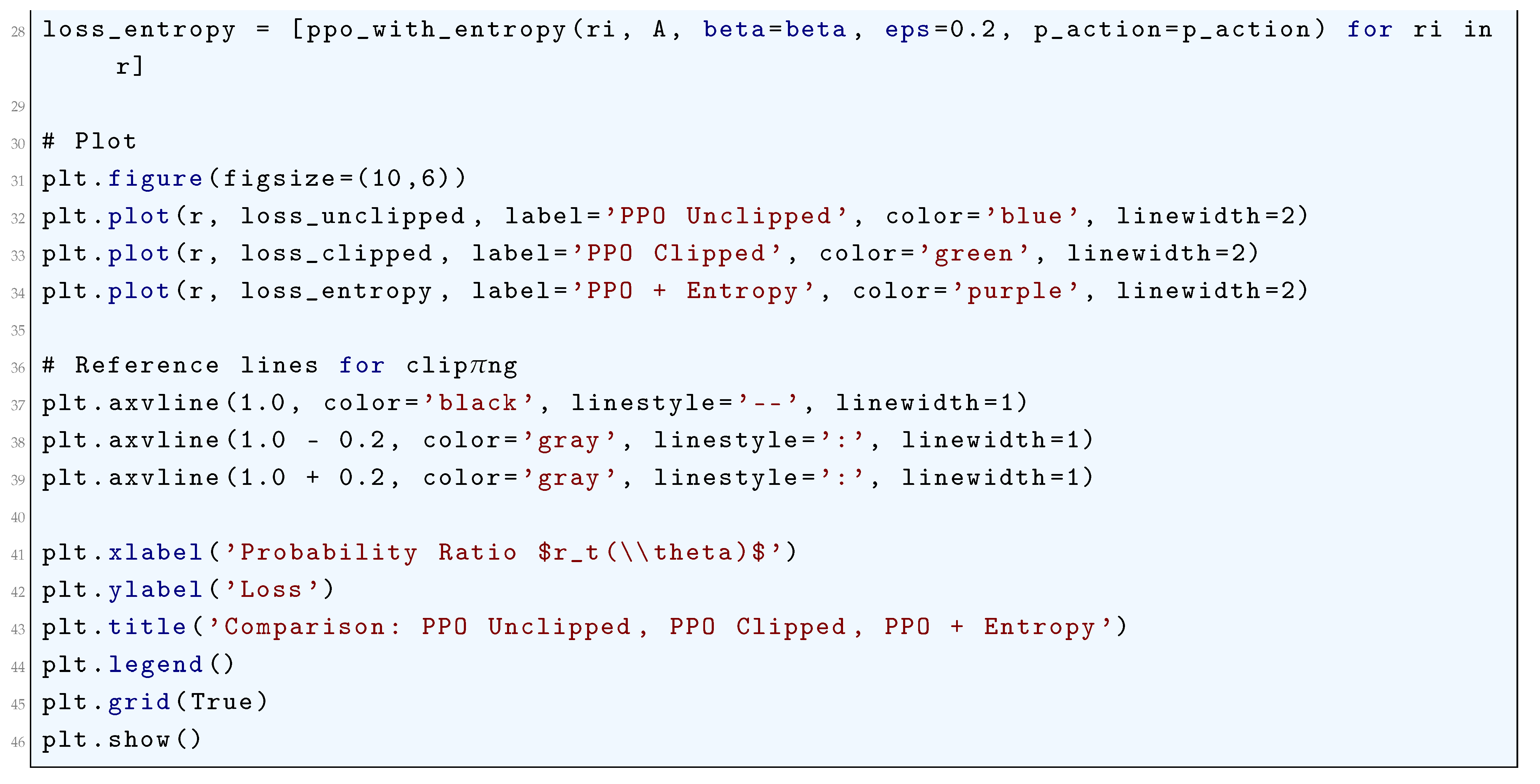
10.5.3.47 Python Code to Generate Figure 114 Illustrating Soft Actor-Critic (SAC) Policy Loss with Entropy Regularization
The Python code below produces the Figure 114 illustrating Soft Actor-Critic (SAC) Policy Loss with Entropy Regularization.
Figure 114.
Soft Actor-Critic (SAC) Policy Loss with Entropy Regularization
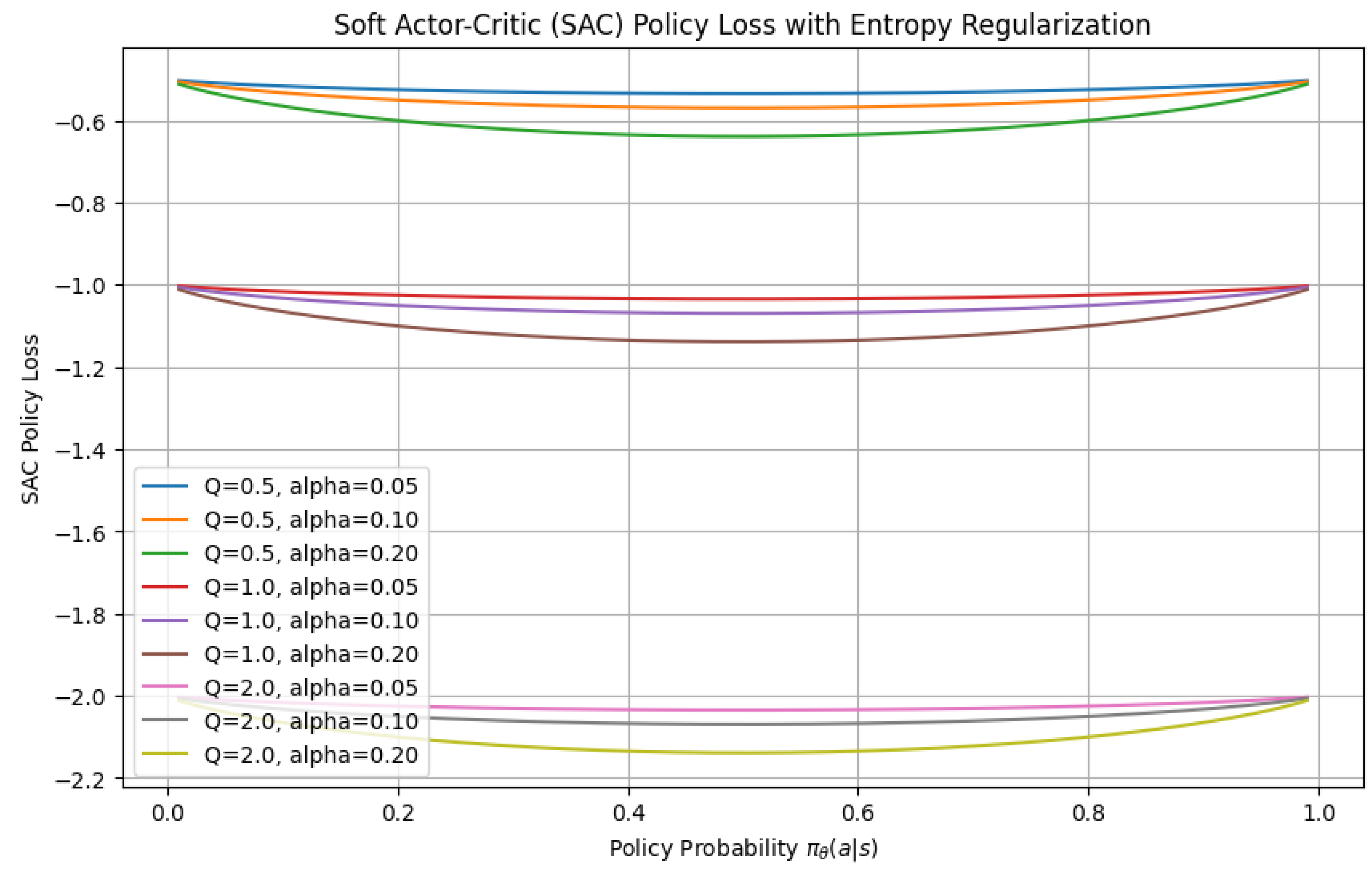
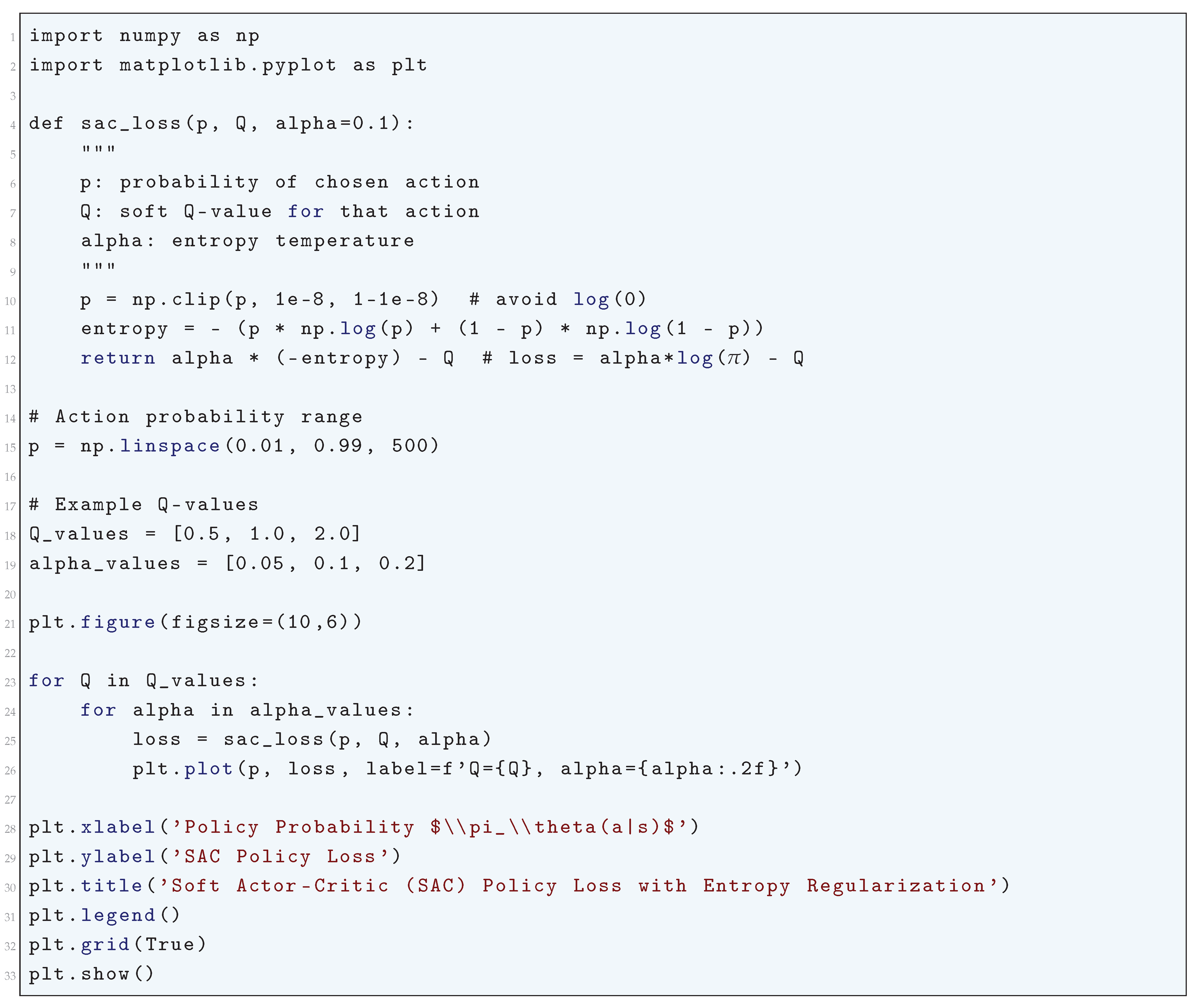
10.5.3.48 Python Code to Generate Figure 115 Illustrating KL Divergence Loss as Sparsity Constraint
The Python code below produces the Figure 115 illustrating KL Divergence Loss as Sparsity Constraint.
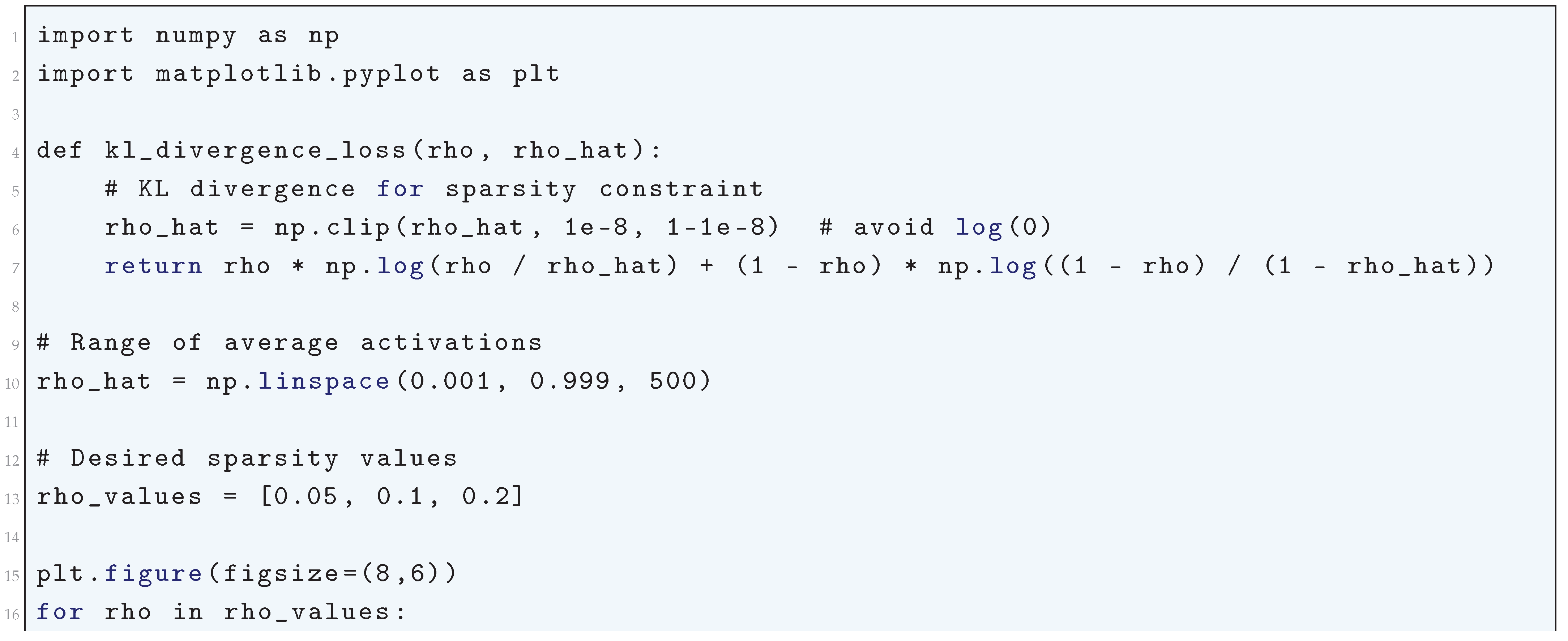
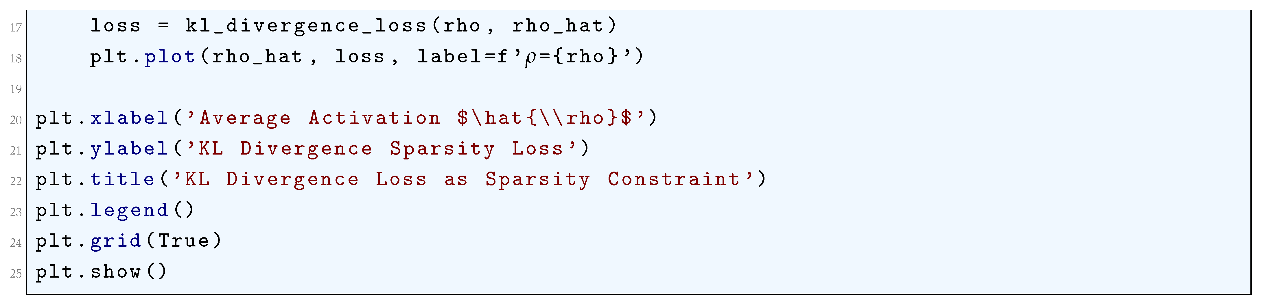
Figure 115.
KL Divergence Loss as Sparsity Constraint
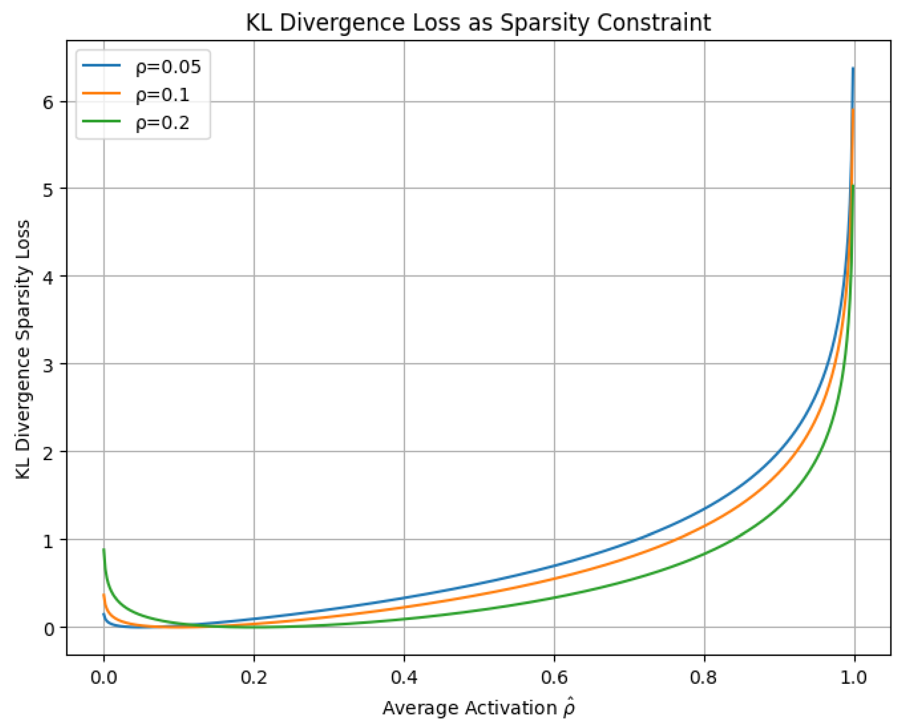
10.5.3.49 Python Code to Generate Figure 116 Illustrating Total KL Sparsity Loss for 10 Hidden Units ()
The Python code below produces the Figure 116 illustrating Total KL Sparsity Loss for 10 Hidden Units ().
Figure 116.
Total KL Sparsity Loss for 10 Hidden Units ()
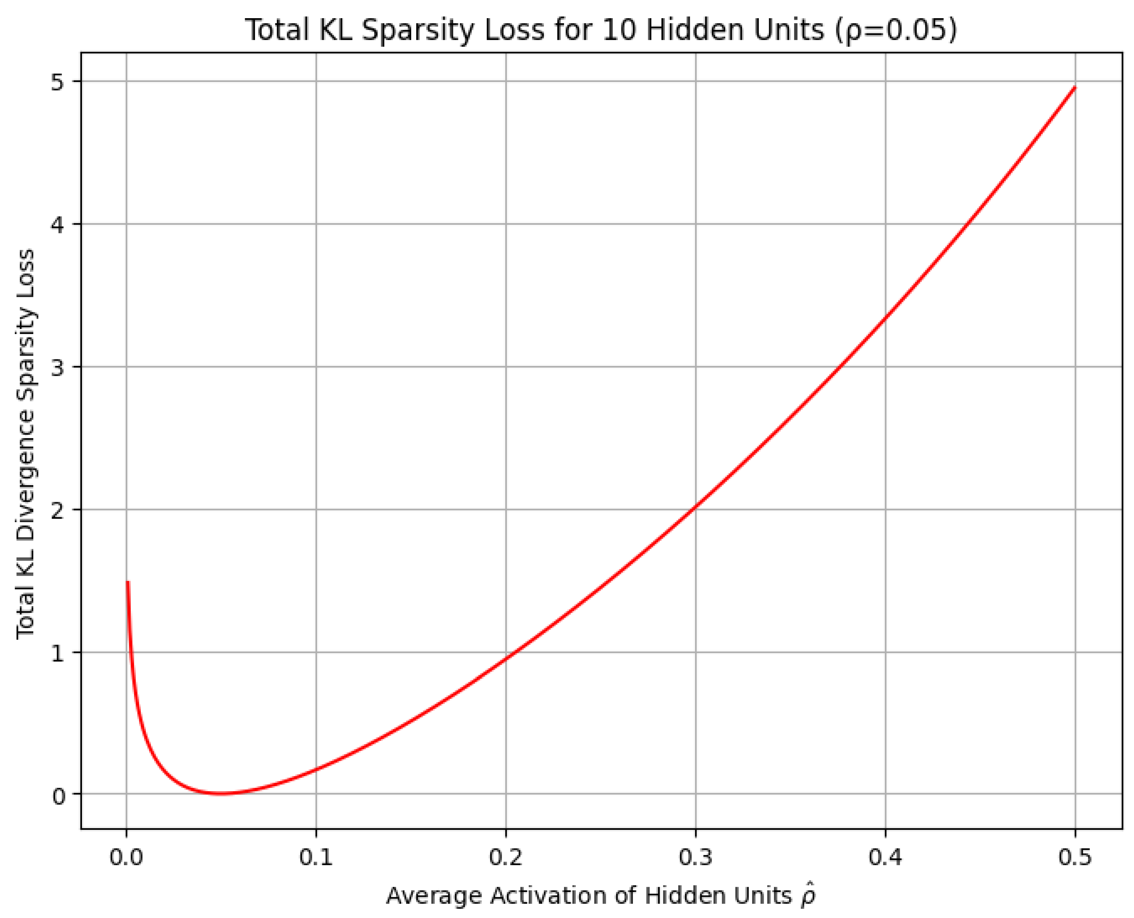
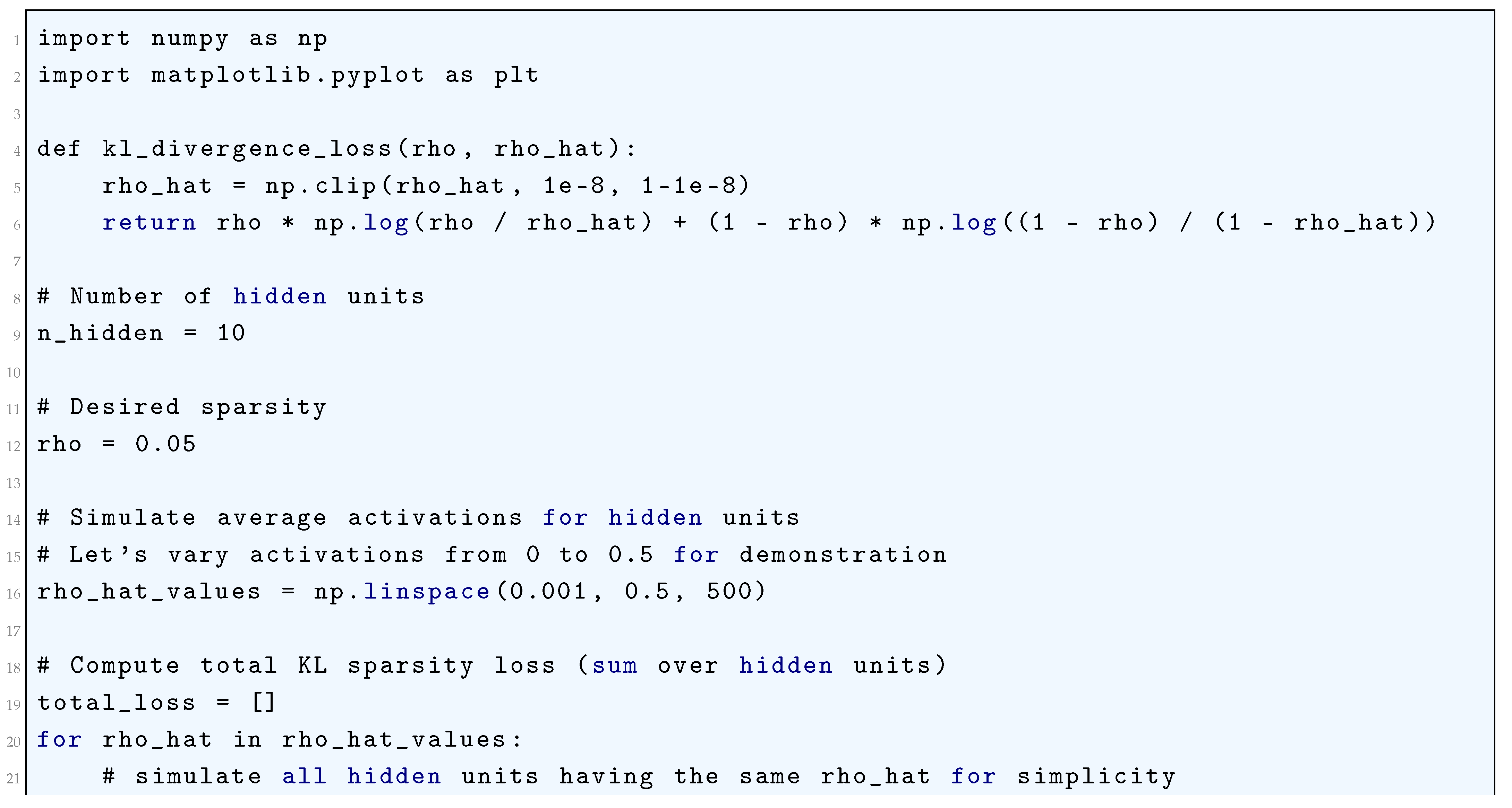
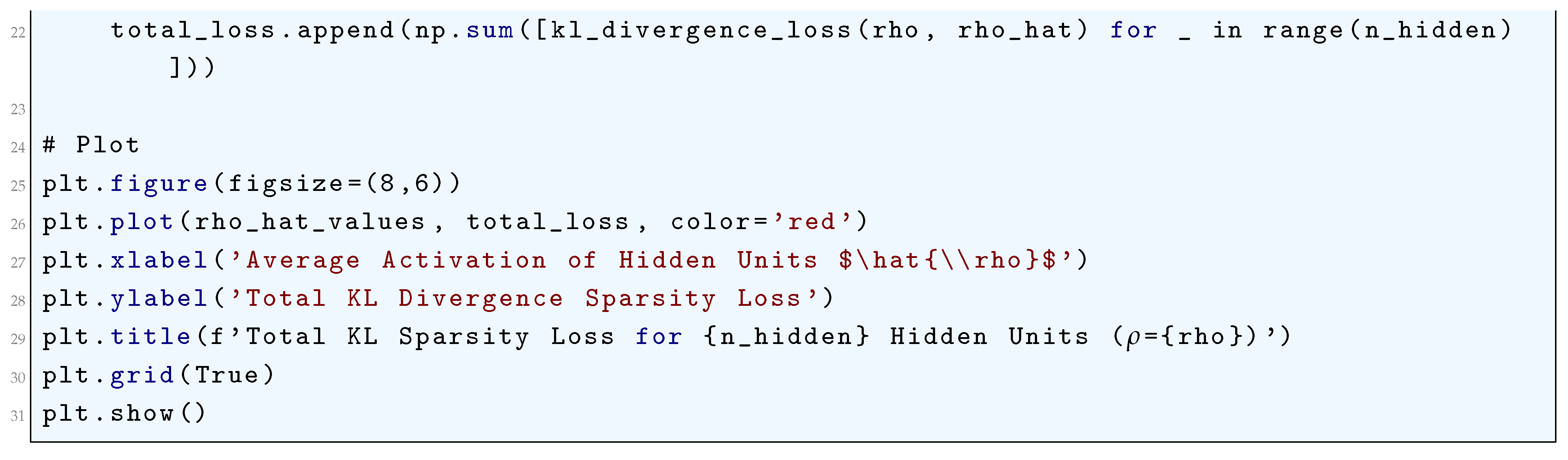
10.5.3.50 Python Code to Generate Figure 117 Illustrating Total KL Sparsity Loss for 10 Hidden Units with Random Activations ()
The Python code below produces the Figure 117 illustrating Total KL Sparsity Loss for 10 Hidden Units with Random Activations ().
Figure 117.
Total KL Sparsity Loss for 10 Hidden Units with Random Activations ()
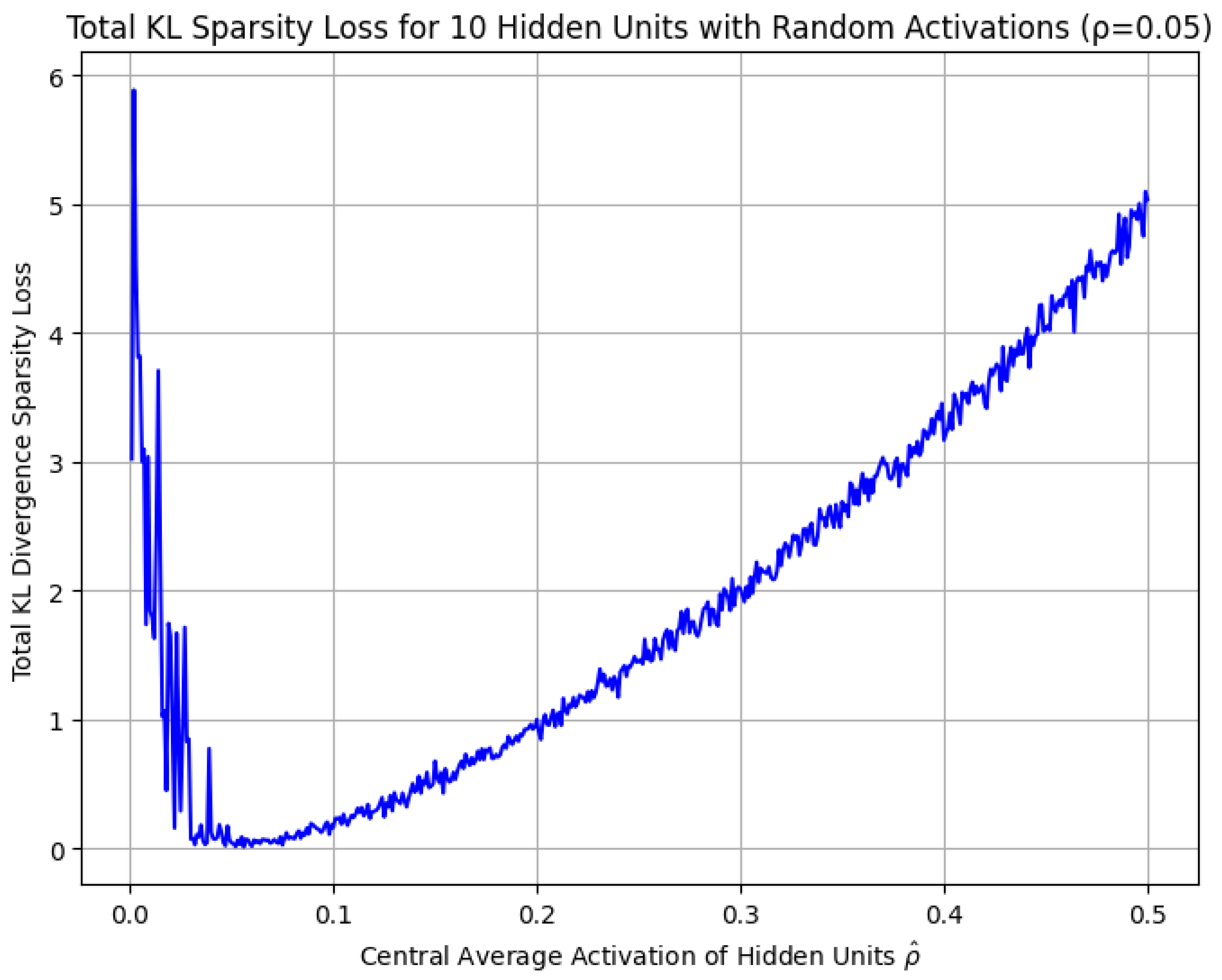
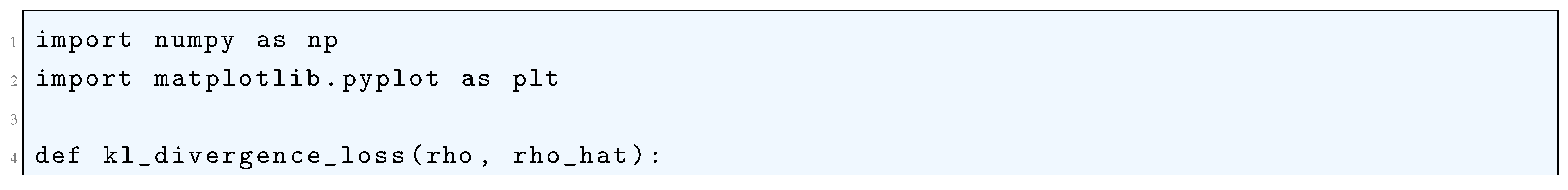
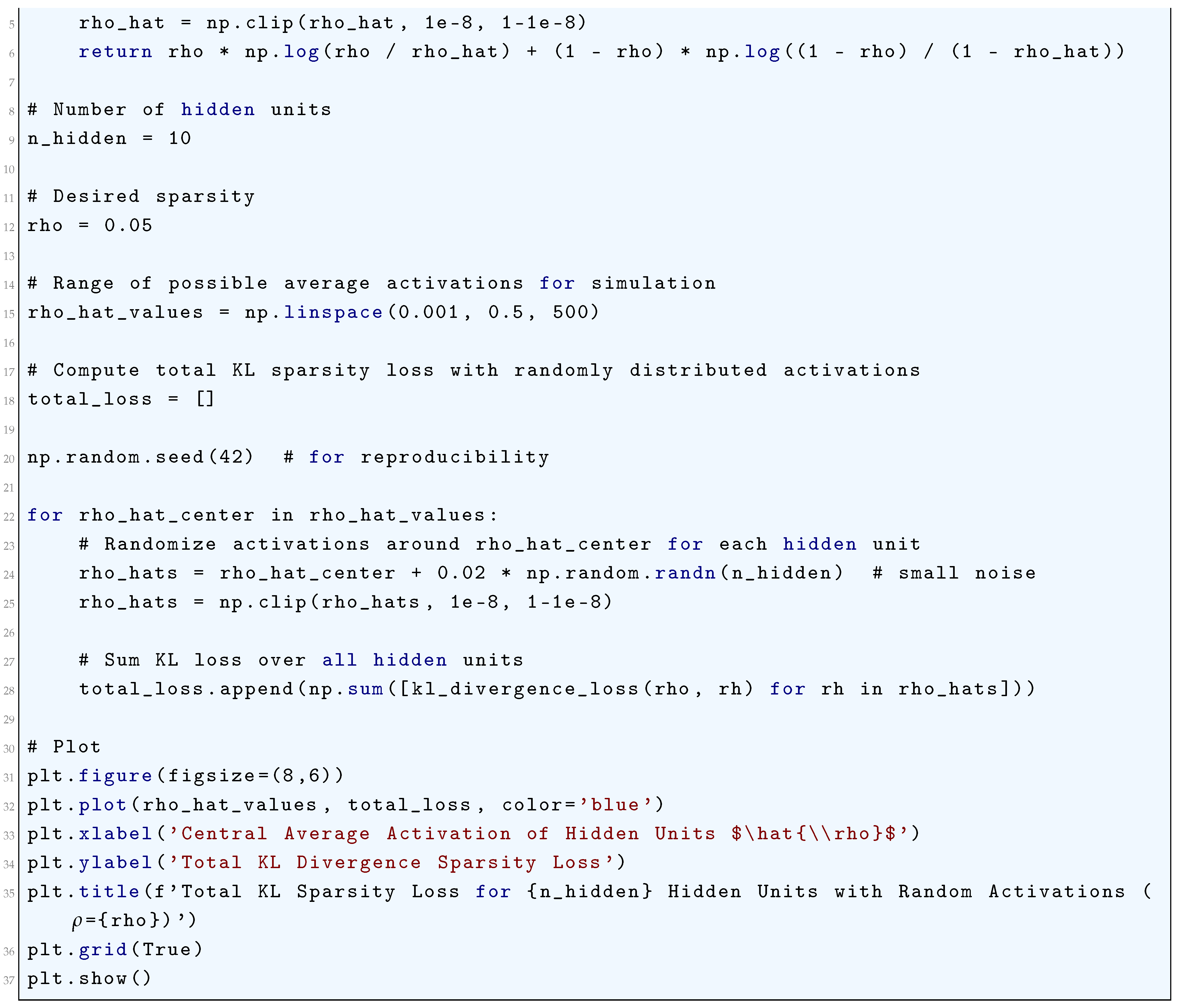
10.5.3.51 Python Code to Generate Figure 118 Illustrating Structured SVM (SSVM) Hinge Loss
The Python code below produces the Figure 118 illustrating Structured SVM (SSVM) Hinge Loss.
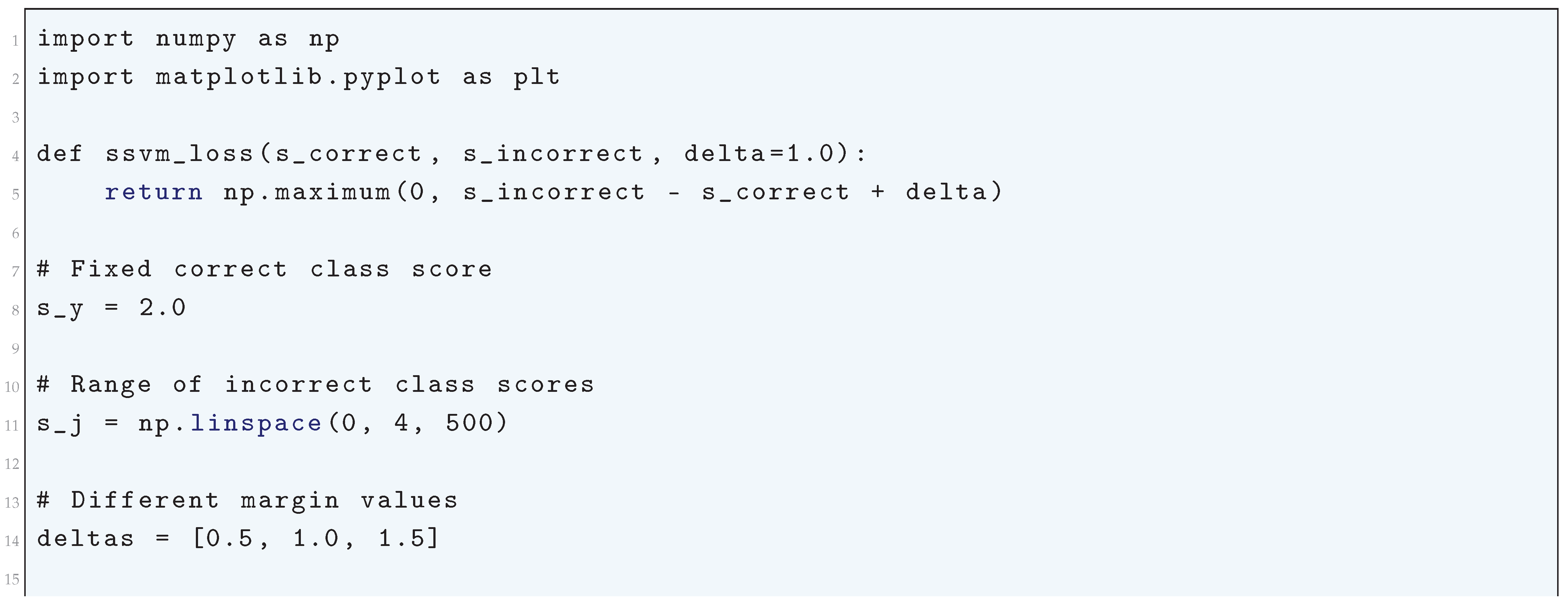
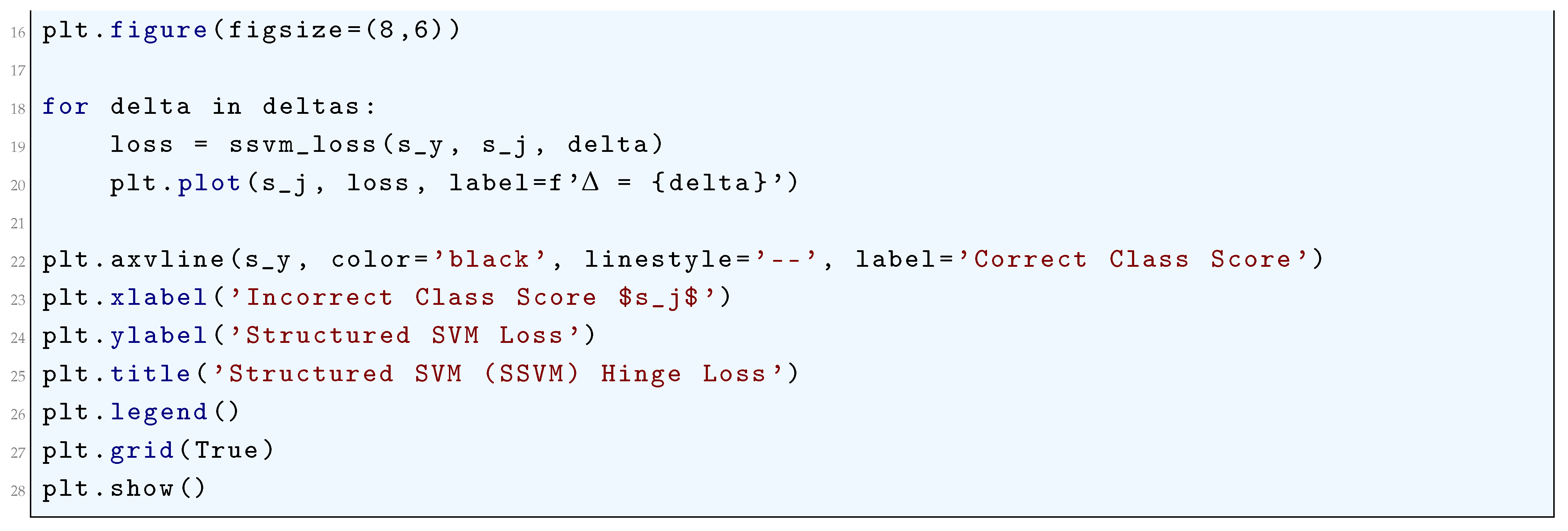
Figure 118.
Structured SVM (SSVM) Hinge Loss
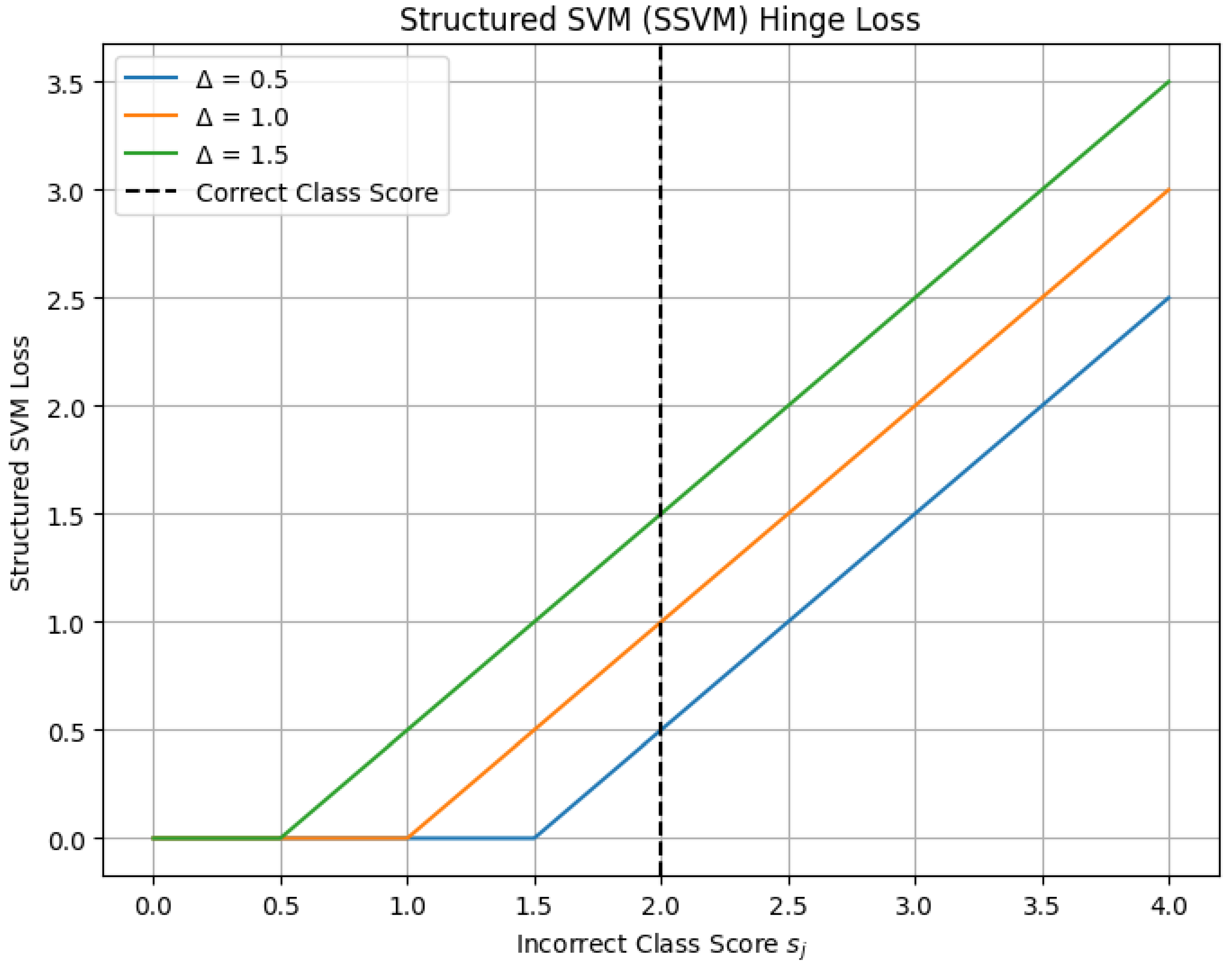
10.5.3.52 Python Code to Generate Figure 119 Illustrating Structured SVM Loss Surface ()
The Python code below produces the Figure 119 illustrating Structured SVM Loss Surface ().
Figure 119.
Structured SVM Loss Surface ()
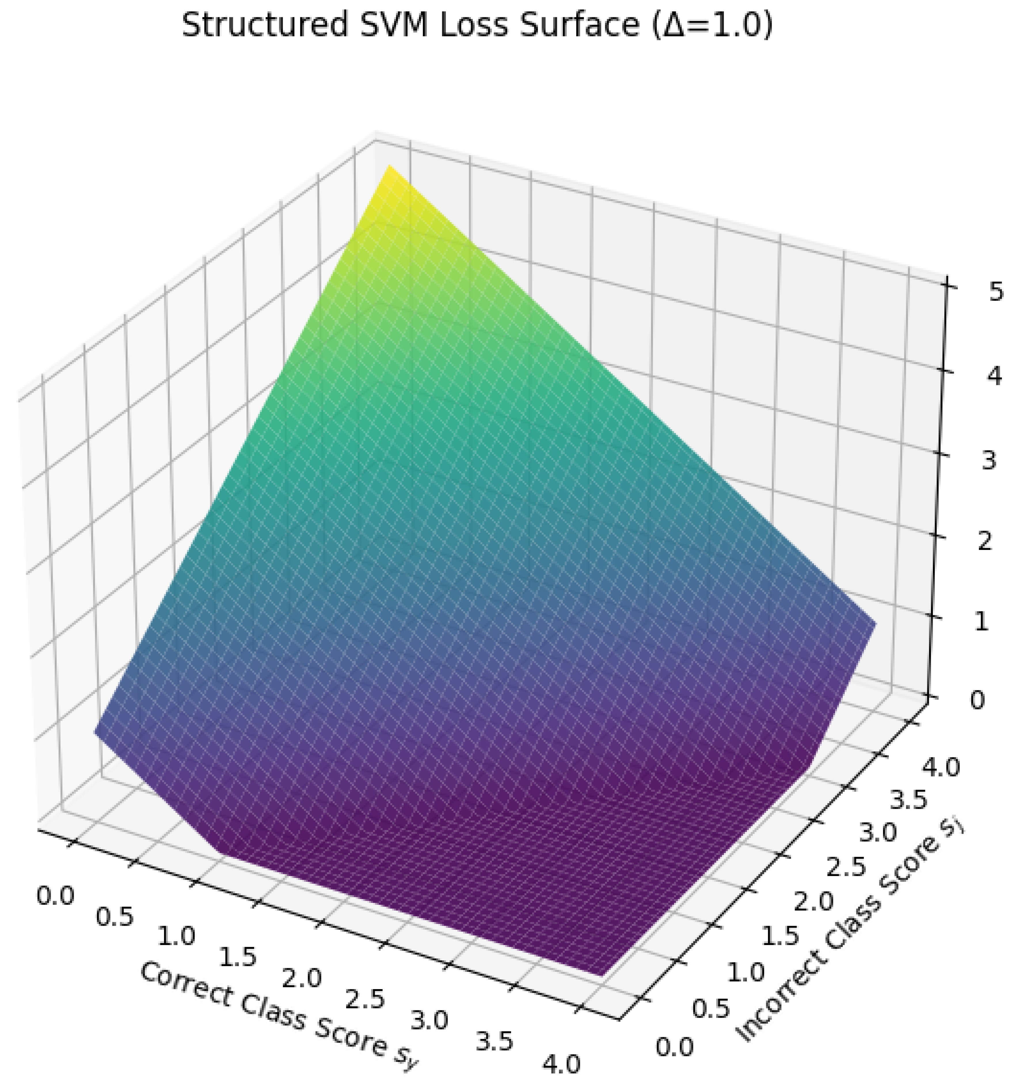
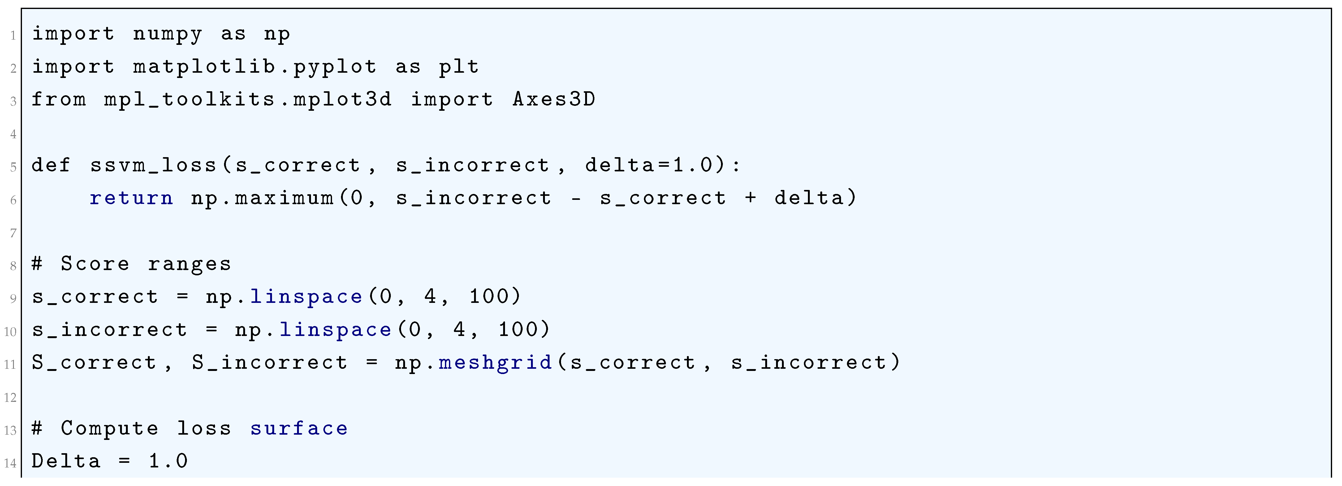
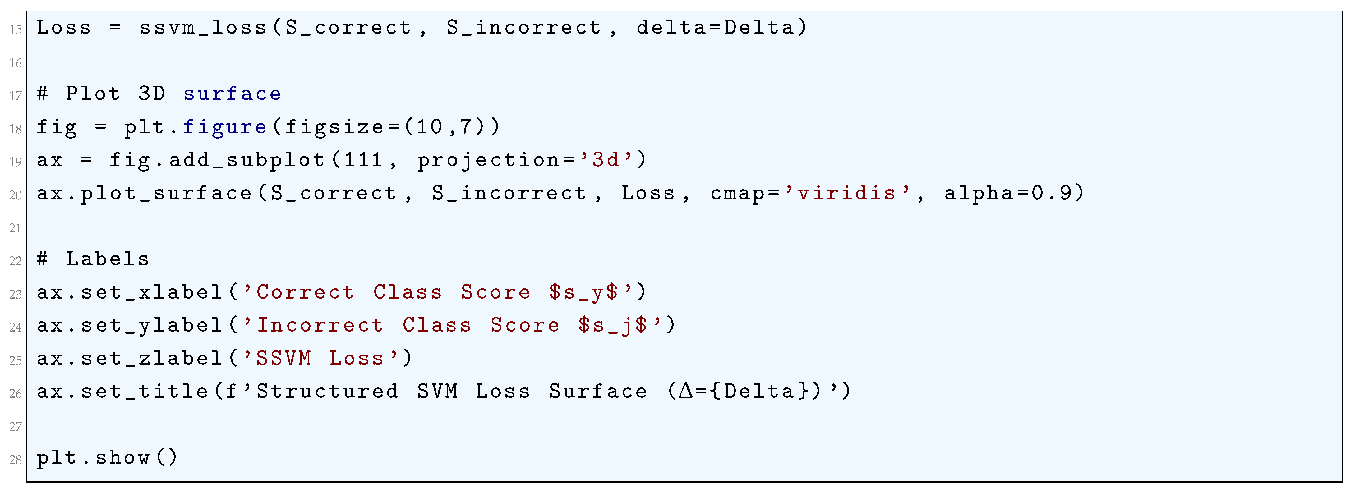
10.5.3.53 Python Code to Generate Figure 120 Illustrating Structured SVM Loss Contour ()
The Python code below produces the Figure 120 illustrating Structured SVM Loss Contour ().
Figure 120.
Structured SVM Loss Contour ()
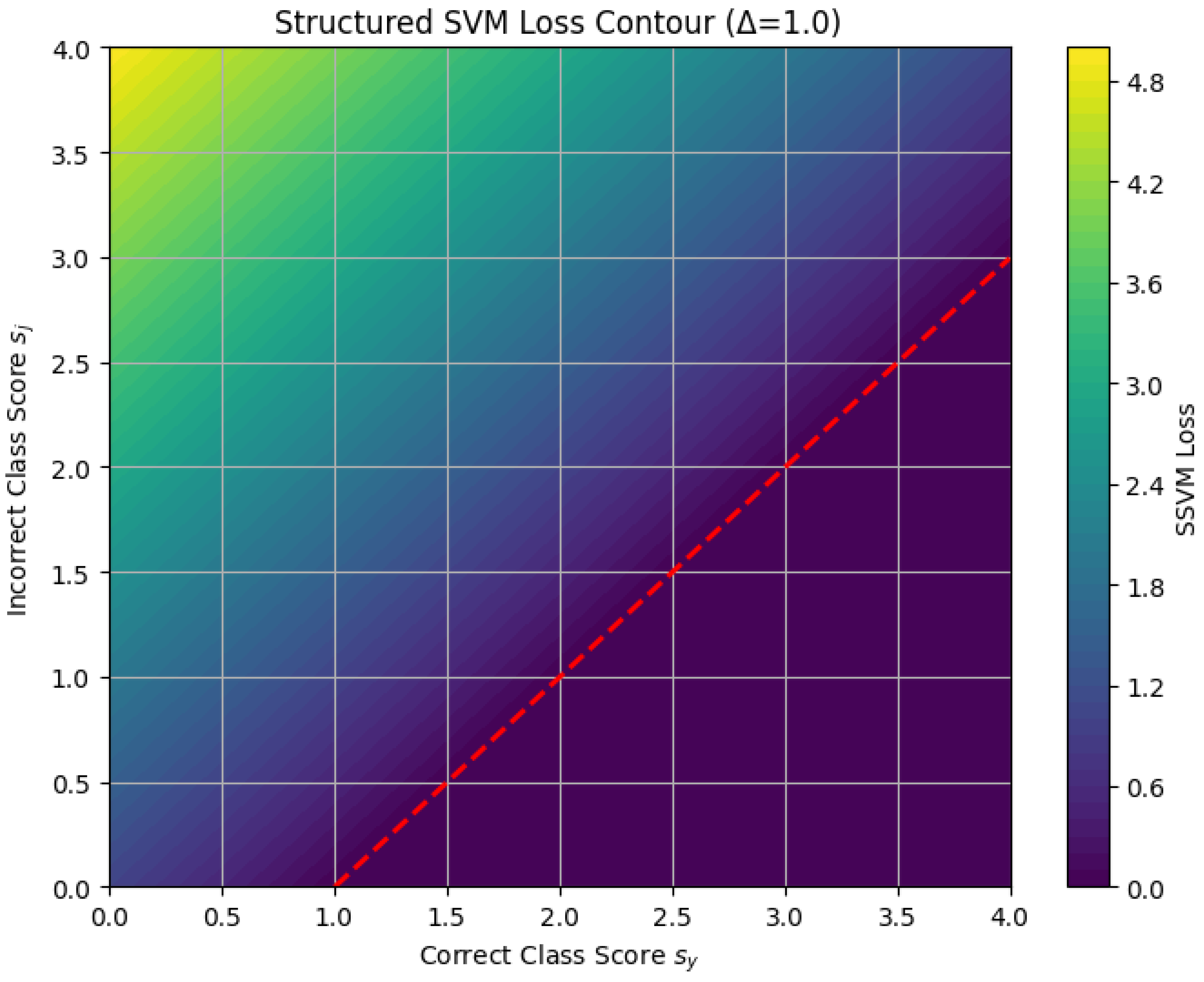
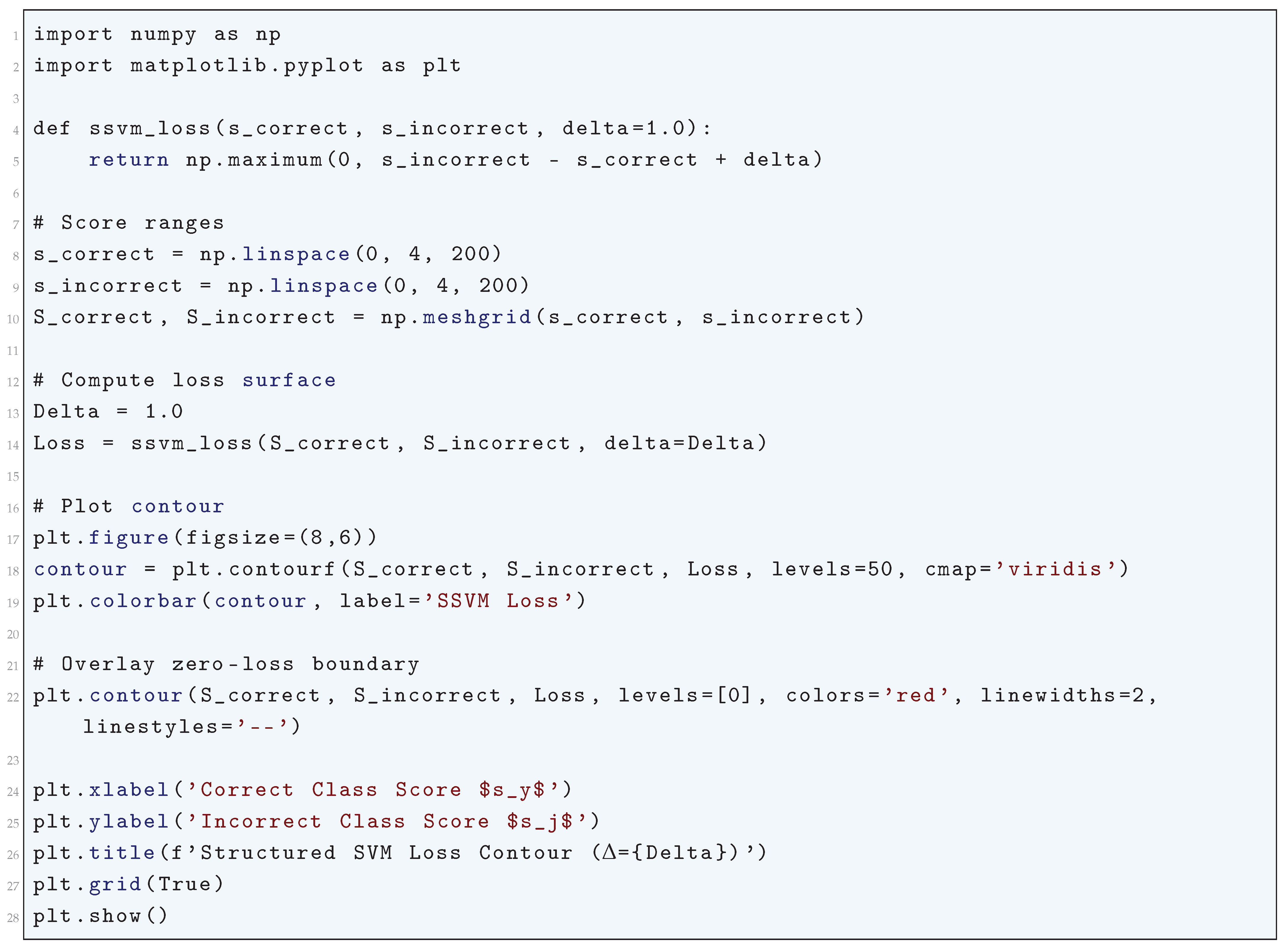
10.5.3.54 Python Code to Generate Figure 121 Illustrating Simplified CRF Loss vs Correct Label Score
The Python code below produces the Figure 121 illustrating Simplified CRF Loss vs Correct Label Score.
Figure 121.
Simplified CRF Loss vs Correct Label Score
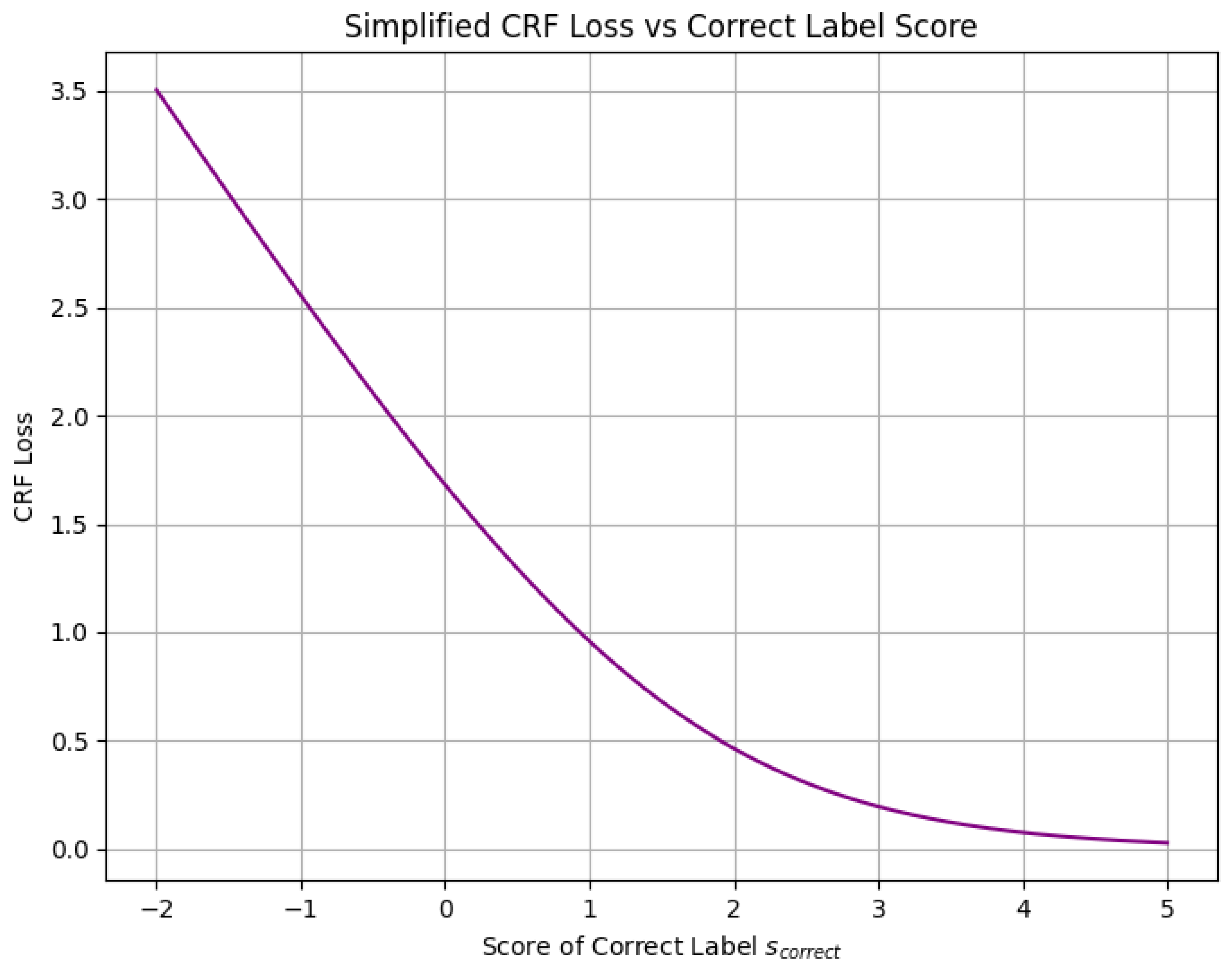
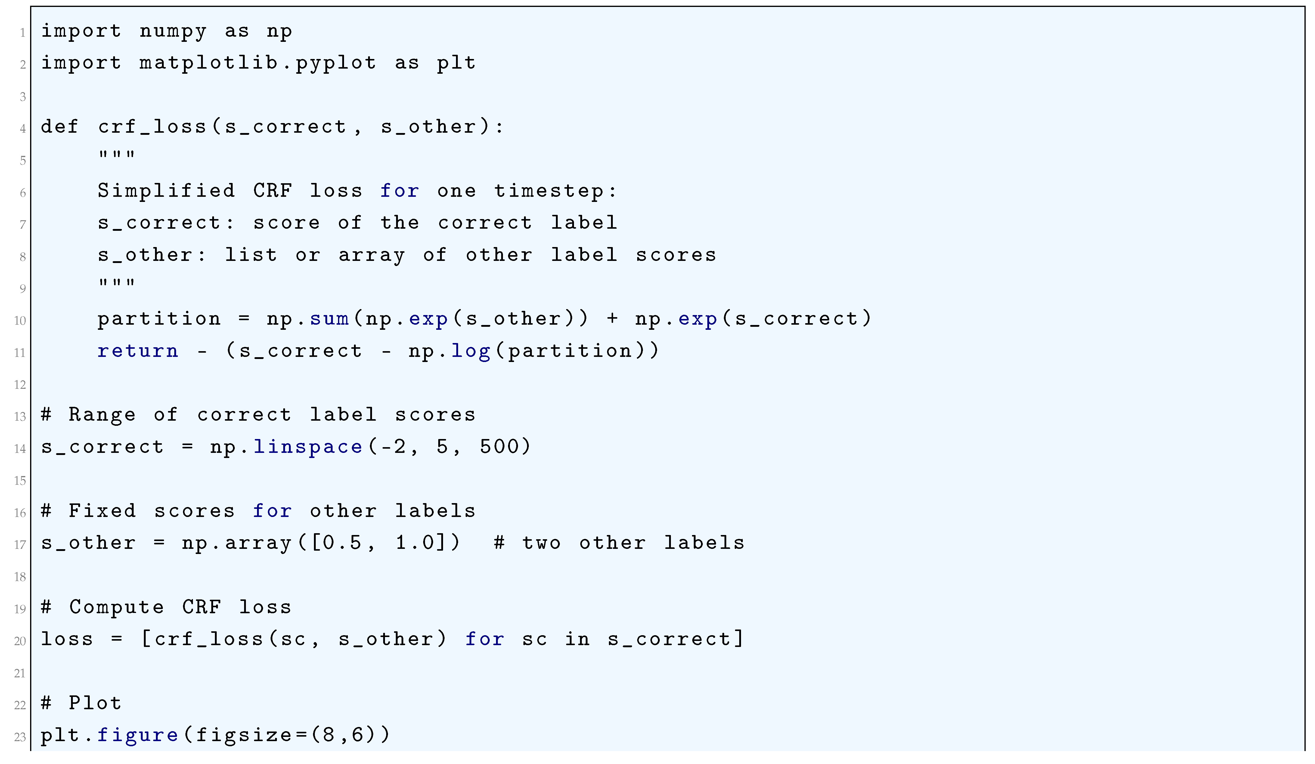
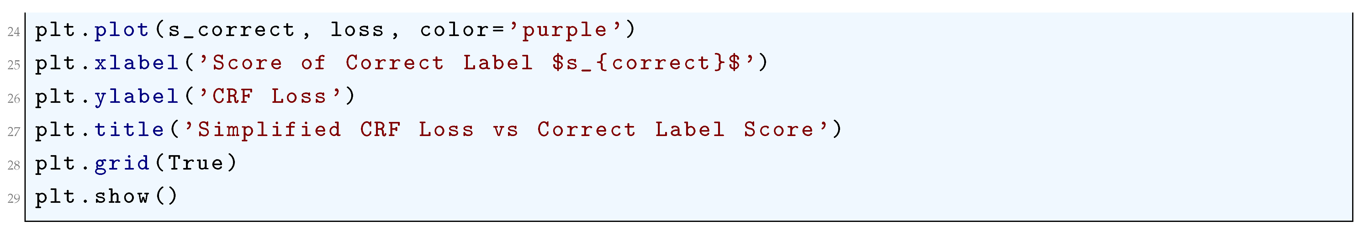
10.5.3.55 Python Code to Generate Figure 122 Illustrating CRF Loss Surface (Single Timestep, 2 Labels)
The Python code below produces the Figure 122 illustrating CRF Loss Surface (Single Timestep, 2 Labels).
Figure 122.
CRF Loss Surface (Single Timestep, 2 Labels)
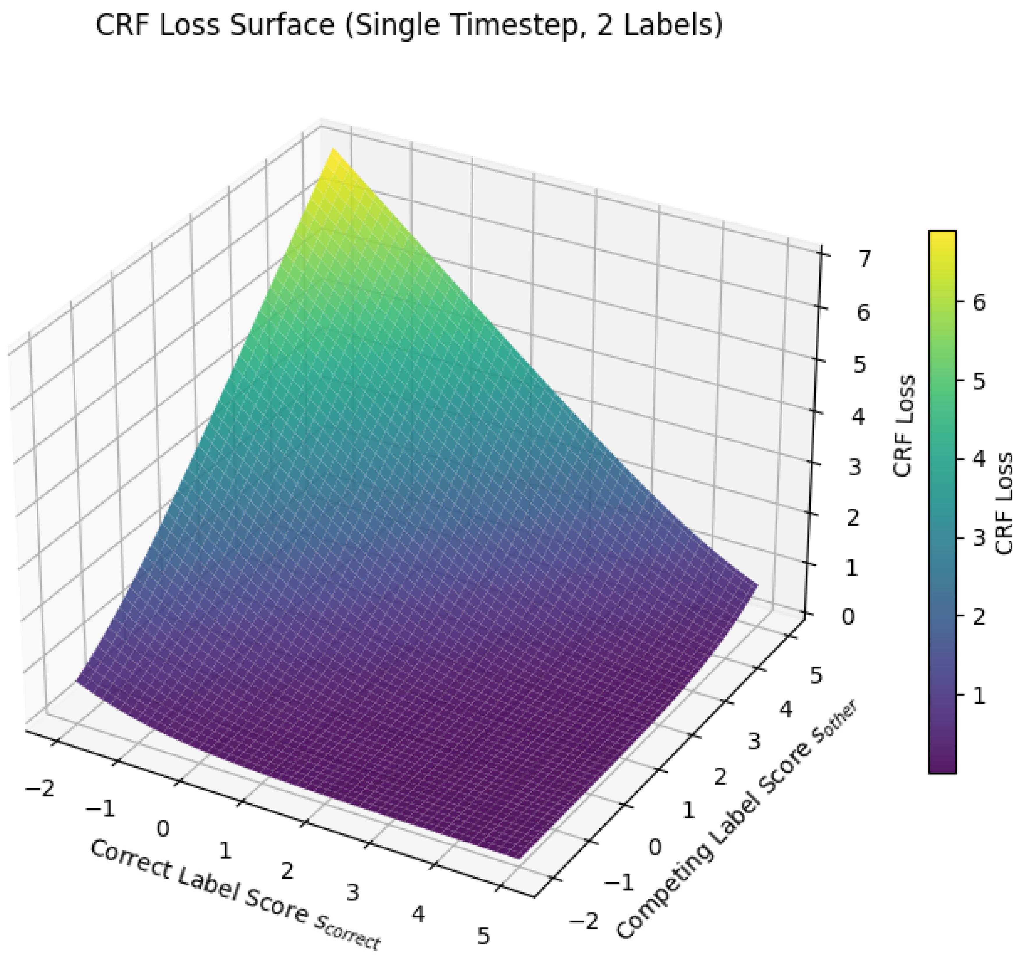
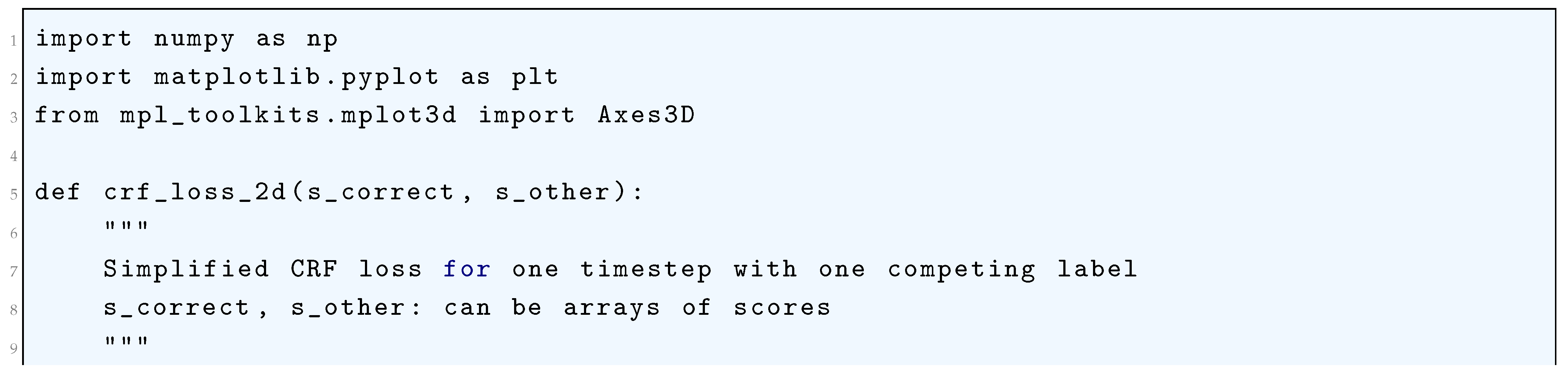
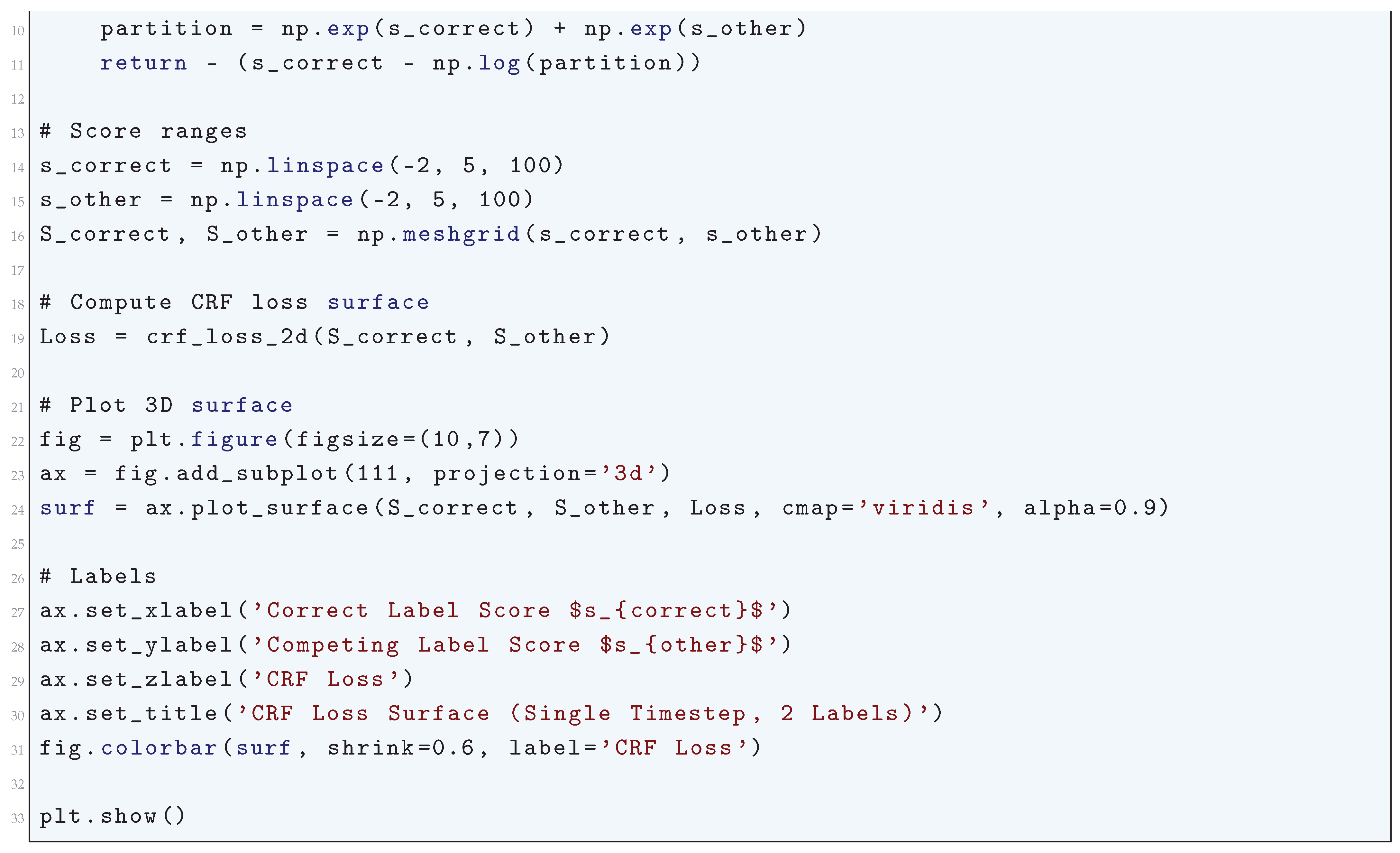
10.5.3.56 Python Code to Generate Figure 123 Illustrating CRF Loss Contour (Single Timestep, 2 Labels)
The Python code below produces the Figure 123 illustrating CRF Loss Contour (Single Timestep, 2 Labels).
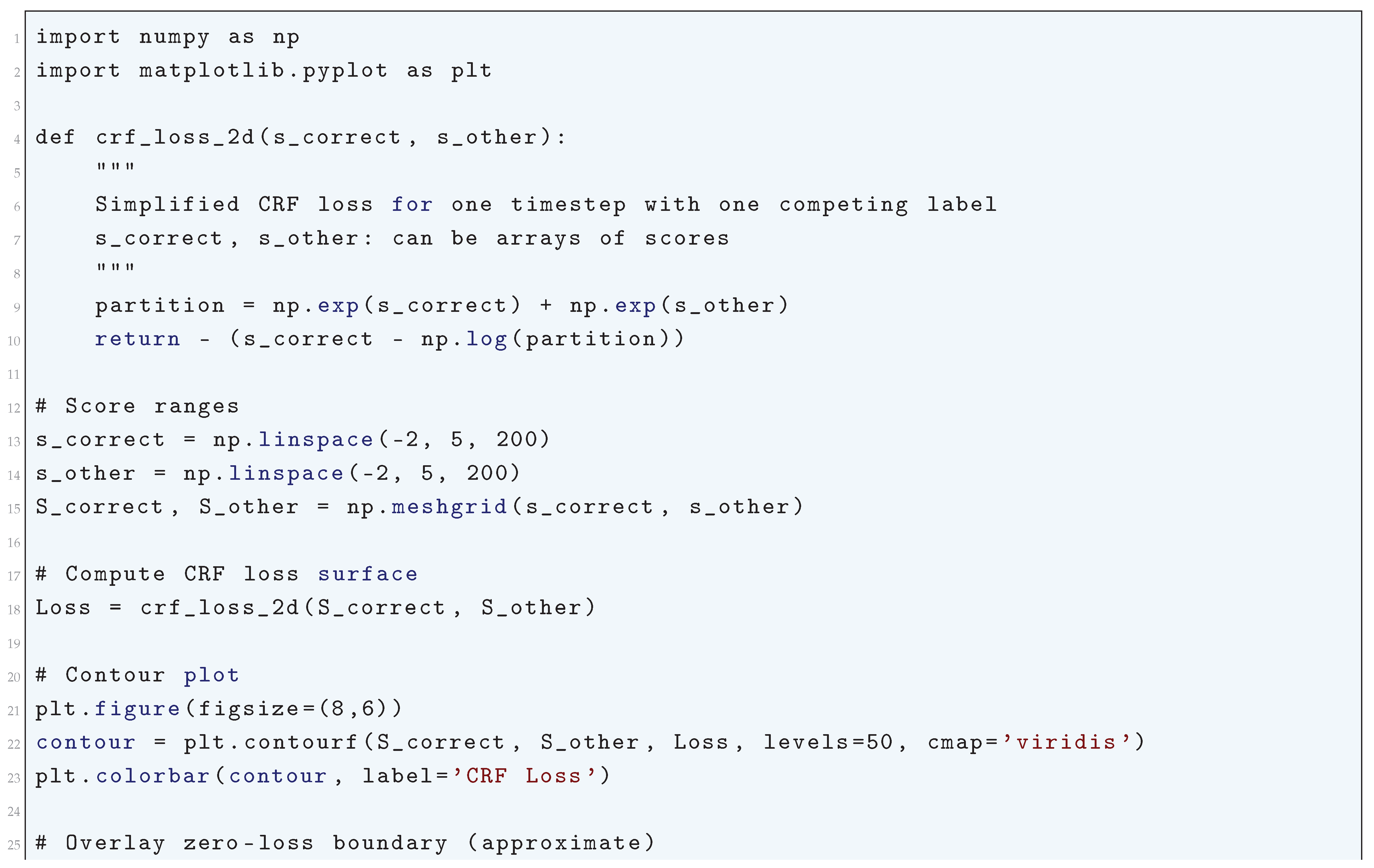
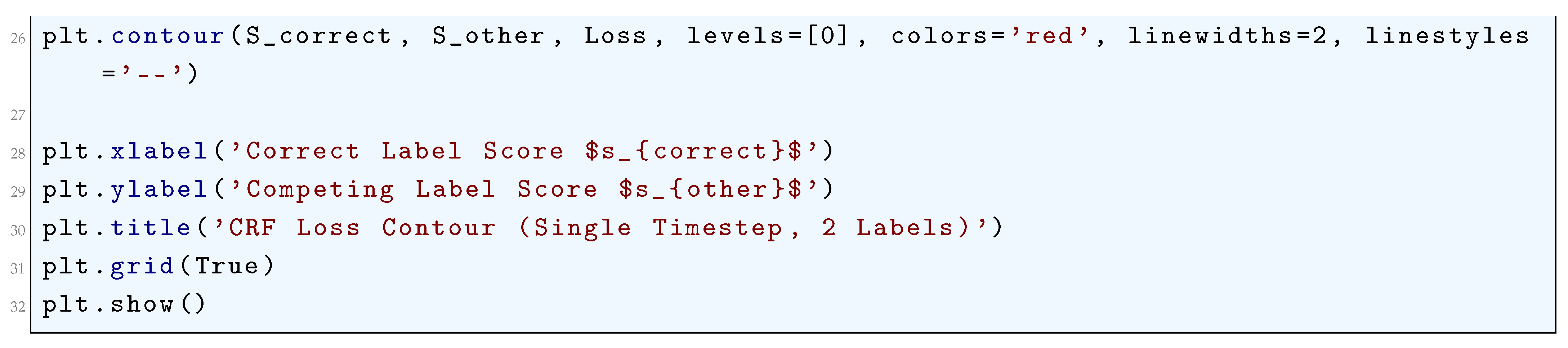
Figure 123.
CRF Loss Contour (Single Timestep, 2 Labels)
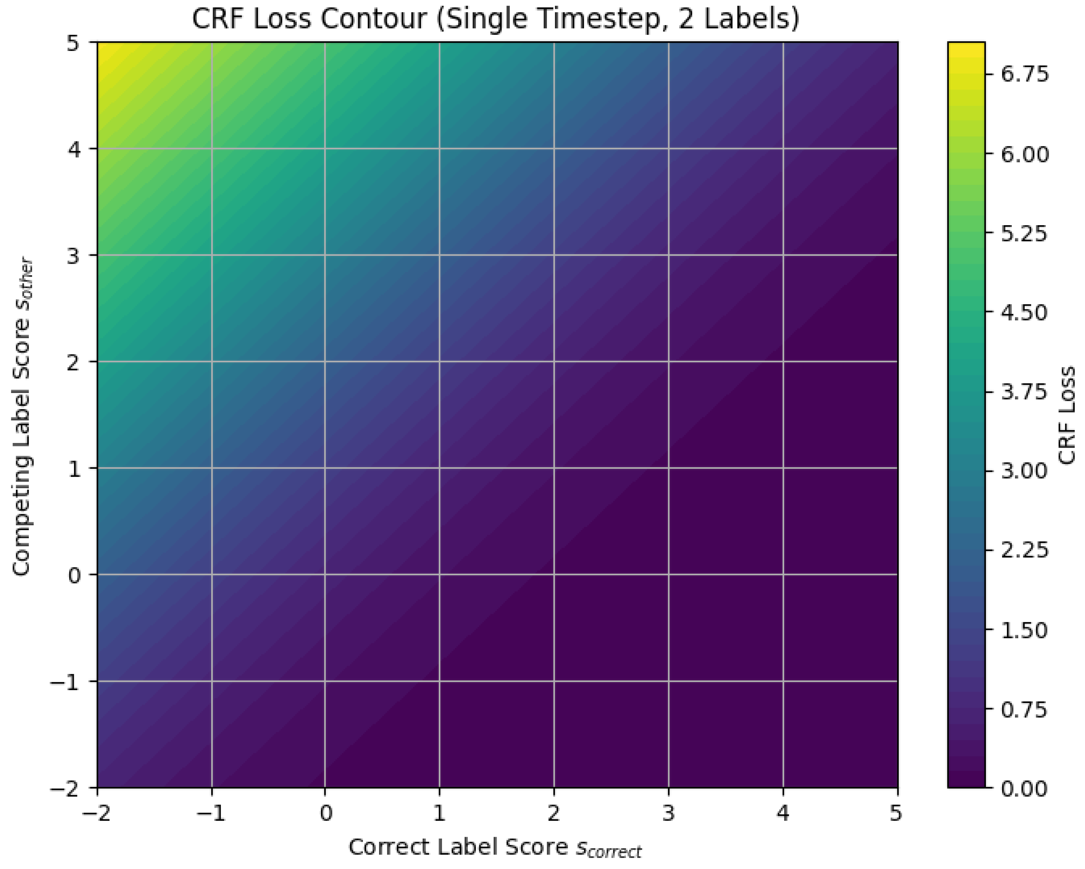
10.5.3.57 Python Code to Generate Figure 124 Illustrating CTC Loss vs Probability of Correct Sequence
The Python code below produces the Figure 124 illustrating CTC Loss vs Probability of Correct Sequence.
Figure 124.
CTC Loss vs Probability of Correct Sequence
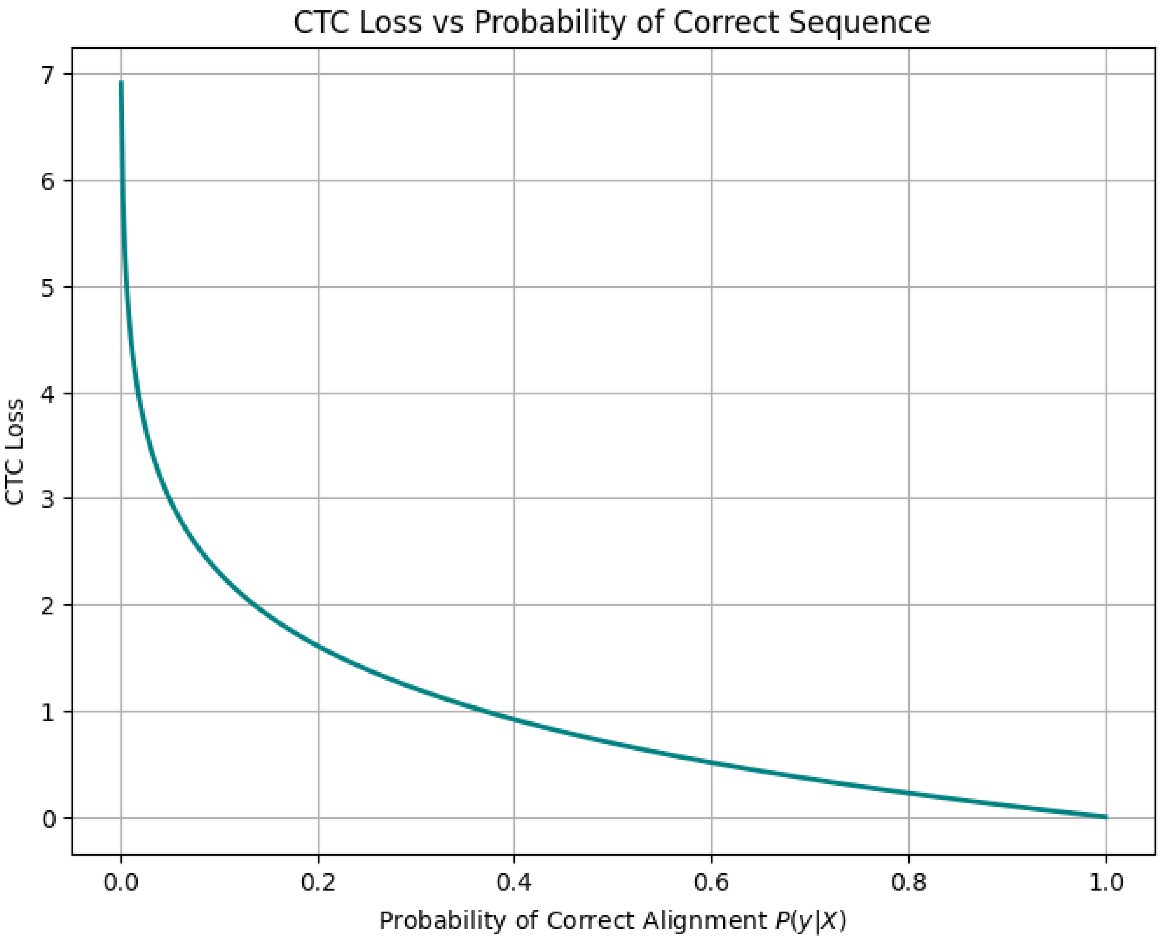
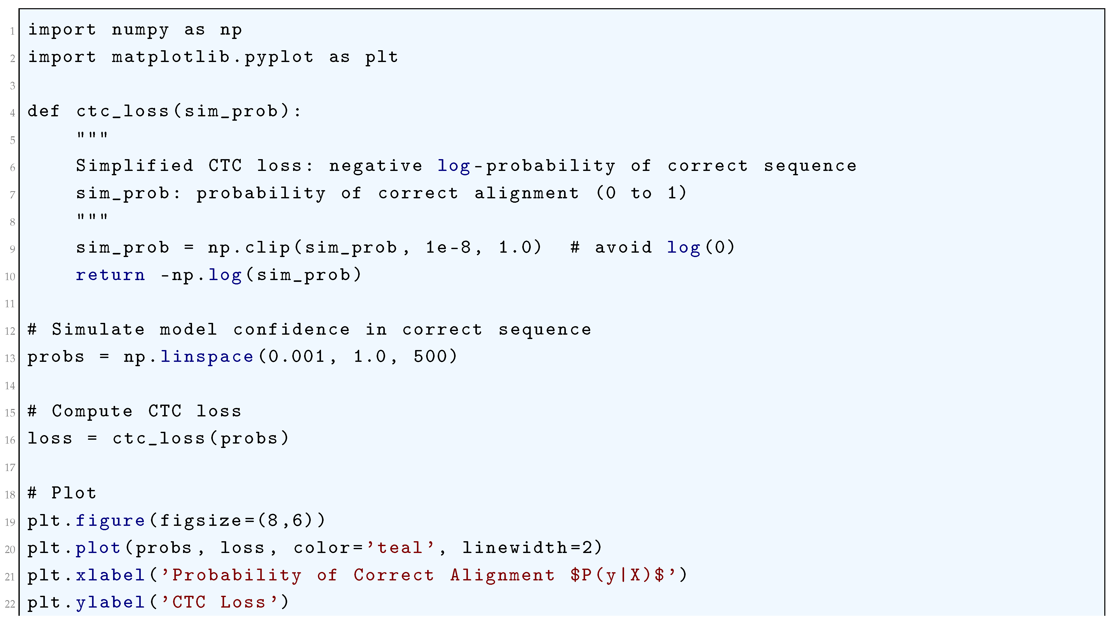

10.5.3.58 Python Code to Generate Figure 125 Illustrating Approximate CTC Loss vs Per-Timestep Probability for Different Sequence Lengths
The Python code below produces the Figure 125 illustrating Approximate CTC Loss vs Per-Timestep Probability for Different Sequence Lengths.
Figure 125.
Approximate CTC Loss vs Per-Timestep Probability for Different Sequence Lengths
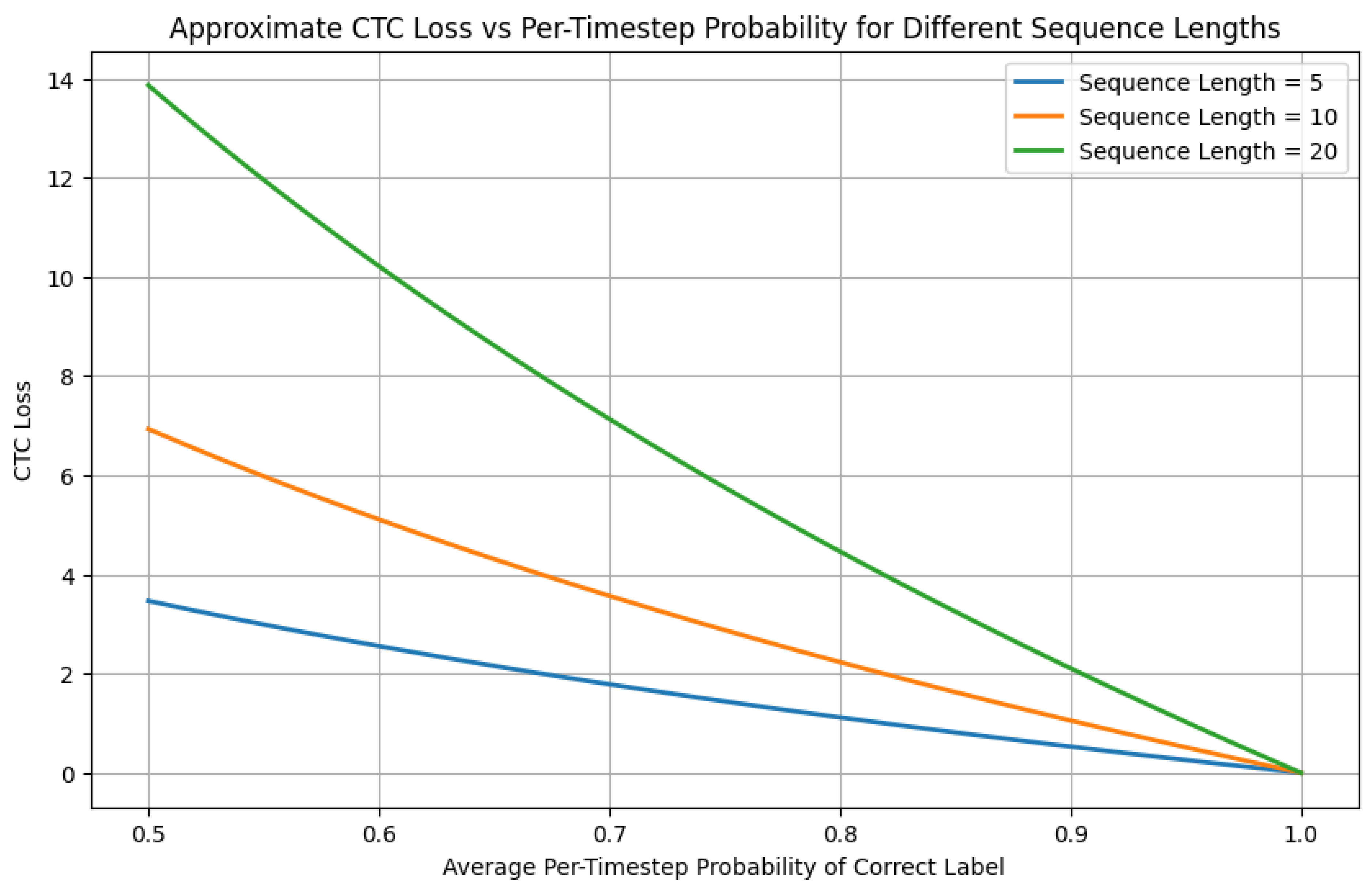
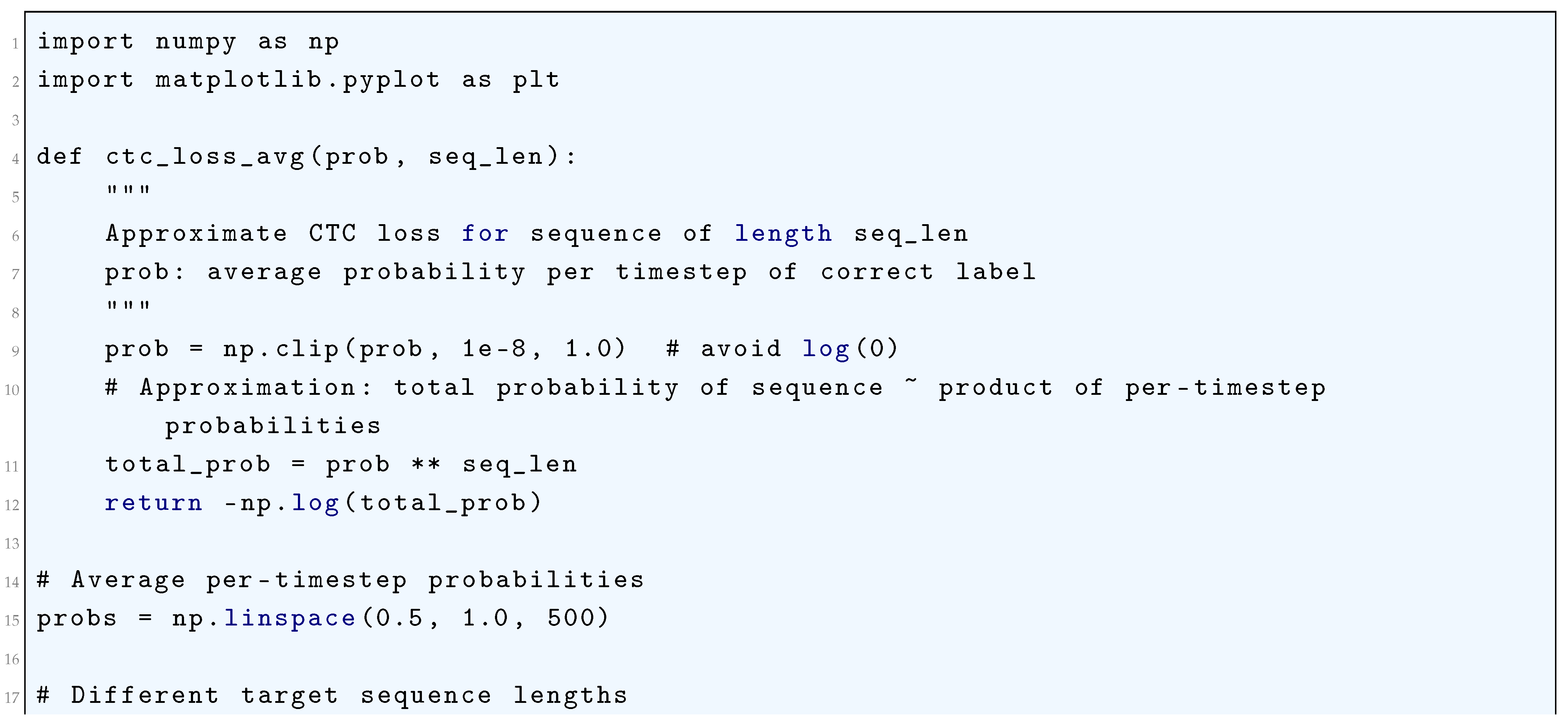
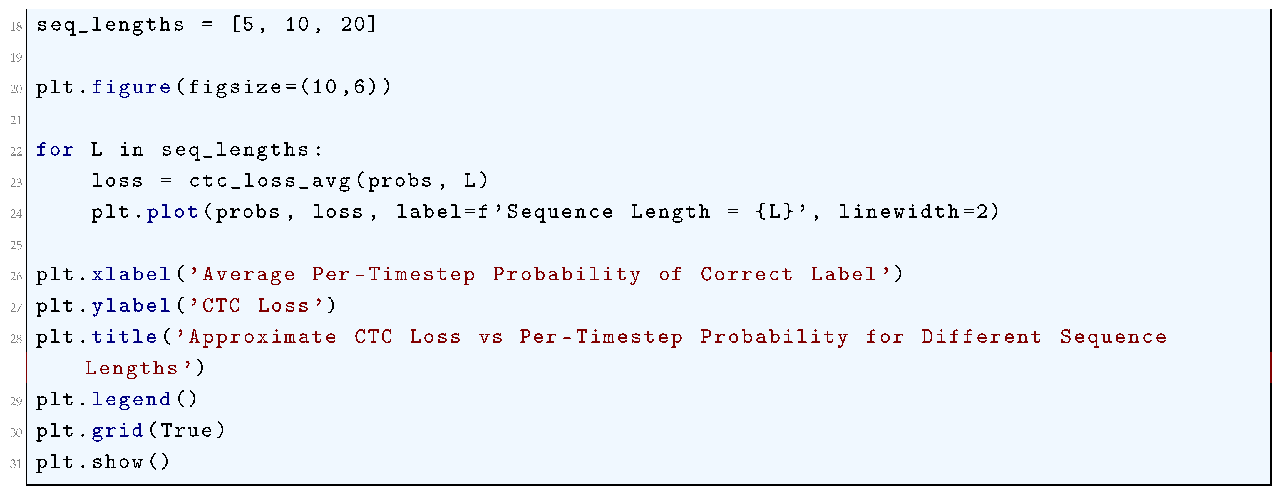
10.5.3.59 Python Code to Generate Figure 126 Illustrating CTC Loss Surface vs Sequence Length and Per-Timestep Probability
The Python code below produces the Figure 126 illustrating CTC Loss Surface vs Sequence Length and Per-Timestep Probability.
Figure 126.
CTC Loss Surface vs Sequence Length and Per-Timestep Probability
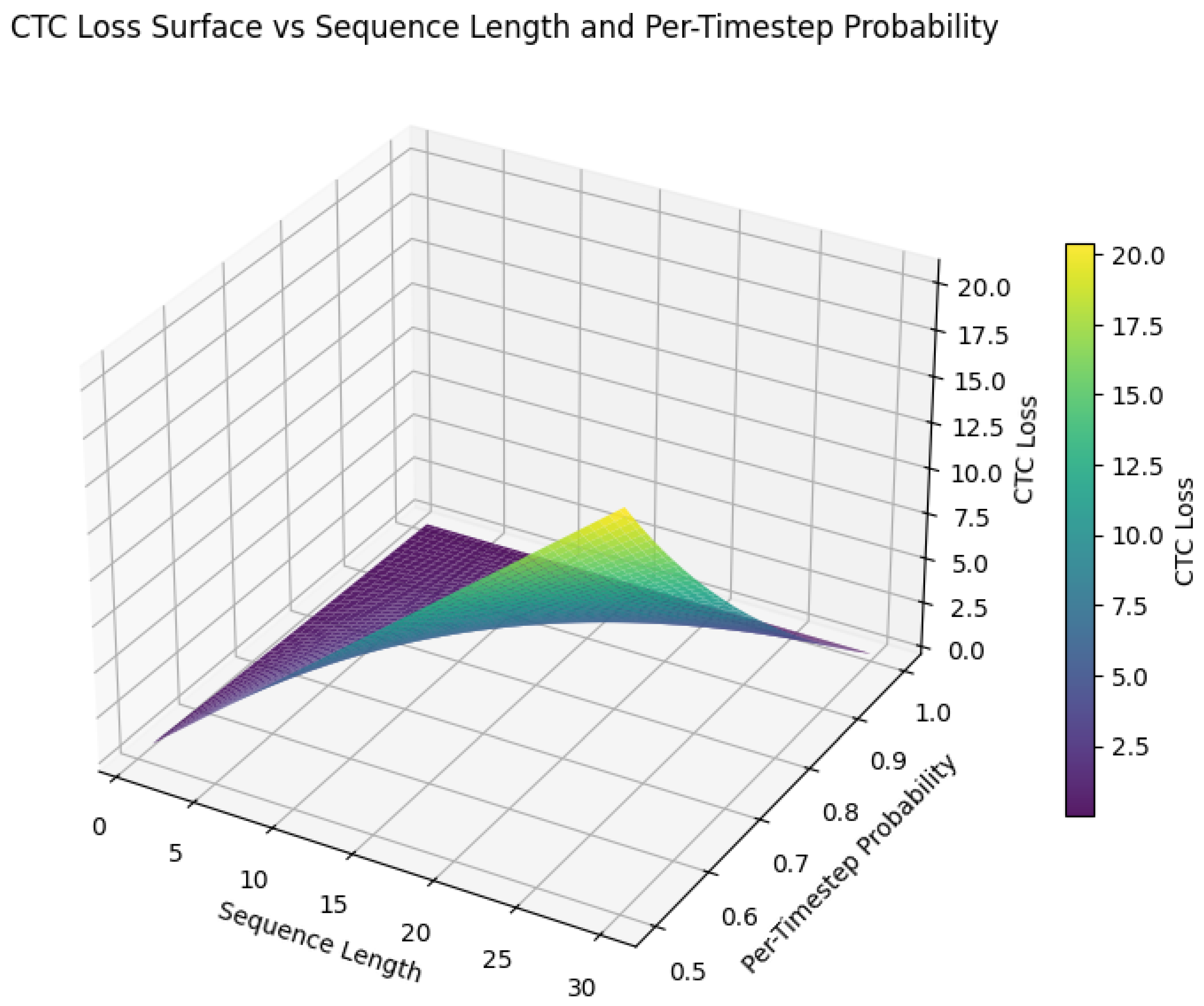
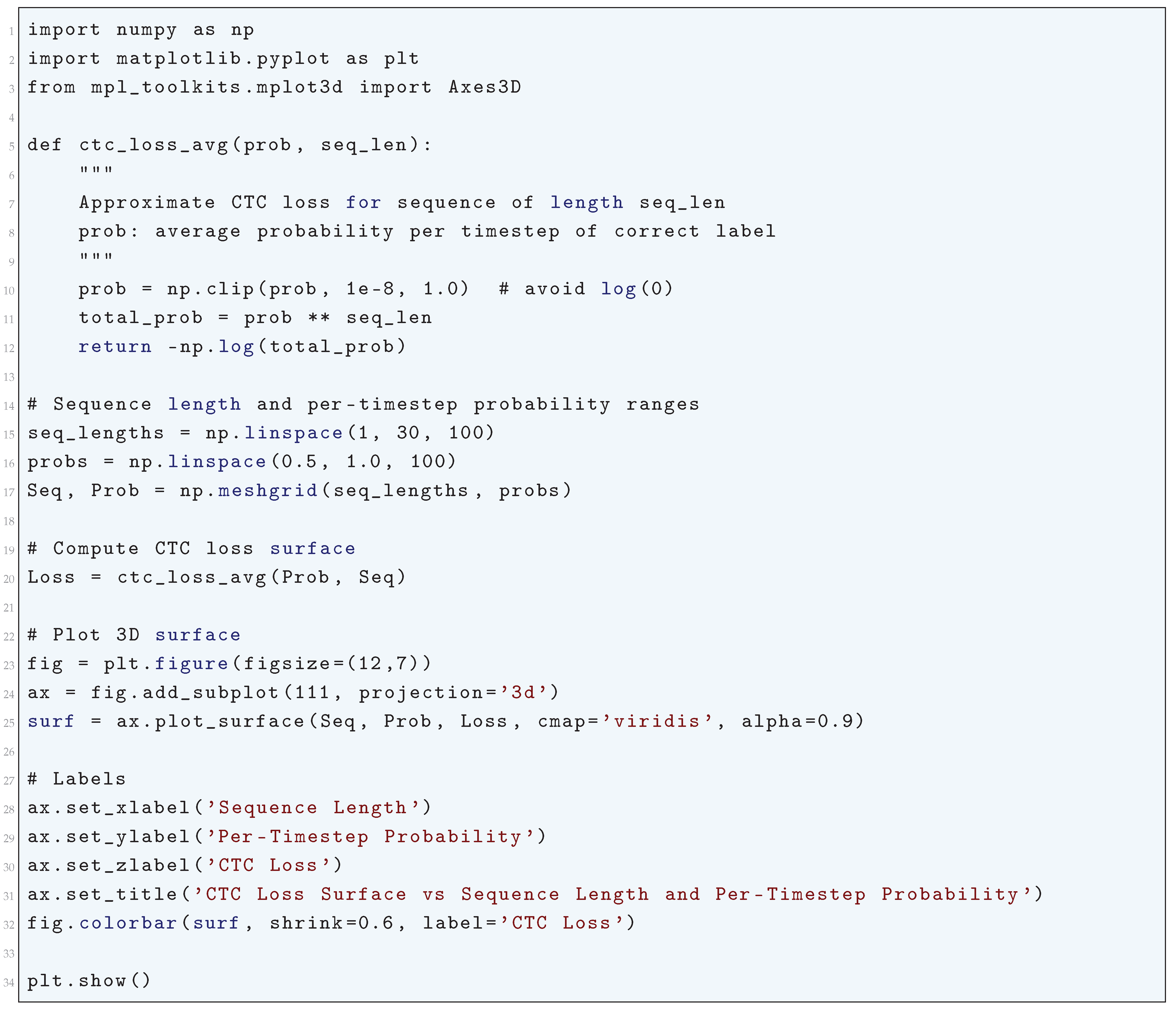
10.5.3.60 Python Code to Generate Figure 127 Illustrating CTC Loss Contour vs Sequence Length and Per-Timestep Probability
The Python code below produces the Figure 127 illustrating CTC Loss Contour vs Sequence Length and Per-Timestep Probability.
Figure 127.
CTC Loss Contour vs Sequence Length and Per-Timestep Probability
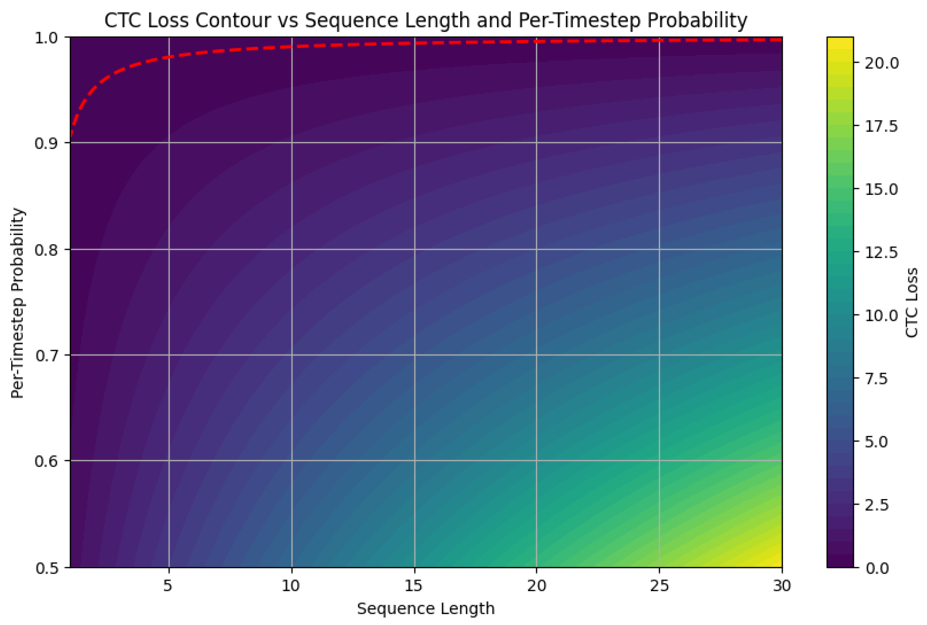
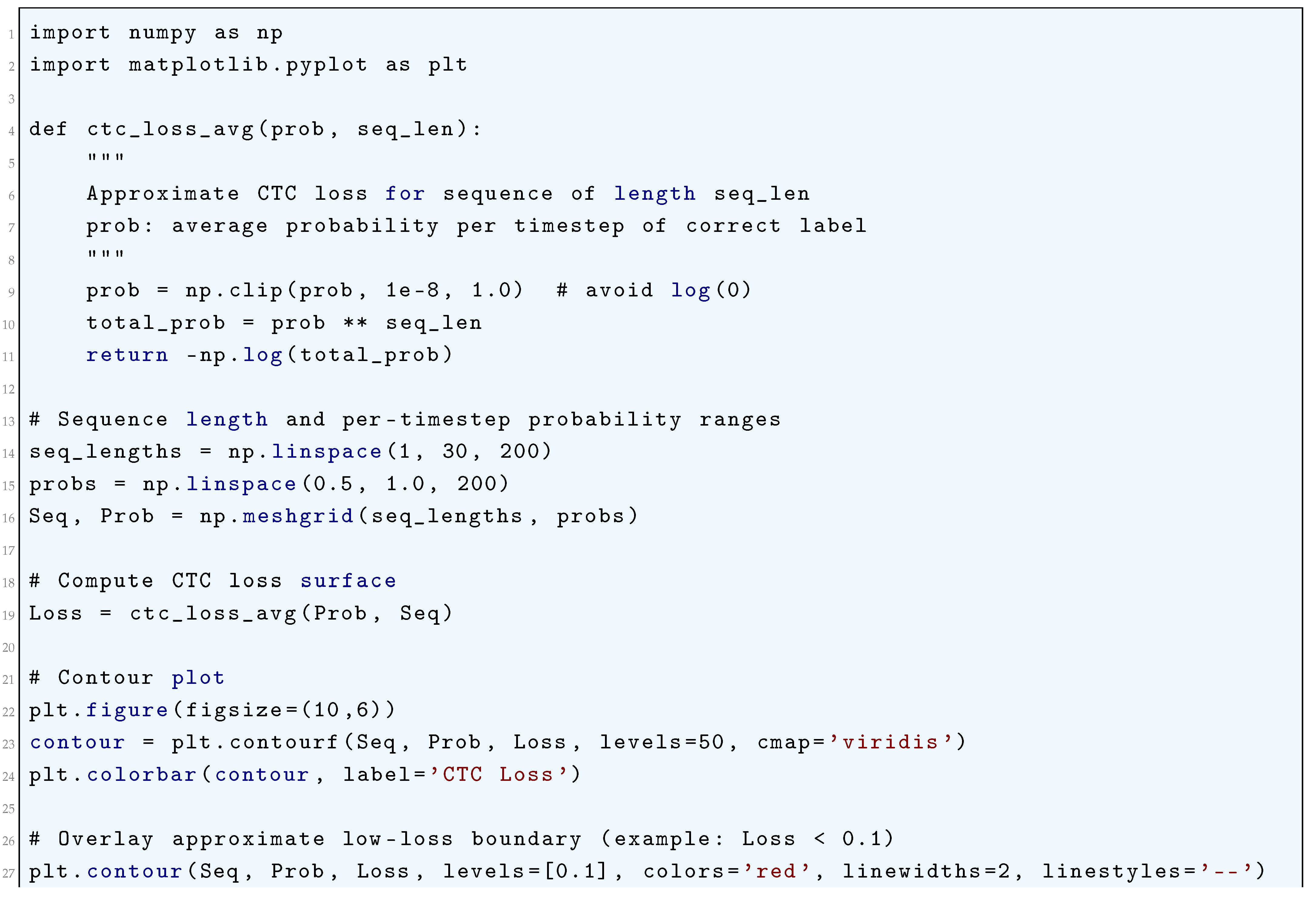
10.5.3.61 Python Code to Generate Figure 128 Illustrating Maximum Margin Markov Networks (M³N) Loss
The Python code below produces the Figure 128 illustrating Maximum Margin Markov Networks (M³N) Loss.
Figure 128.
Maximum Margin Markov Networks (M³N) Loss
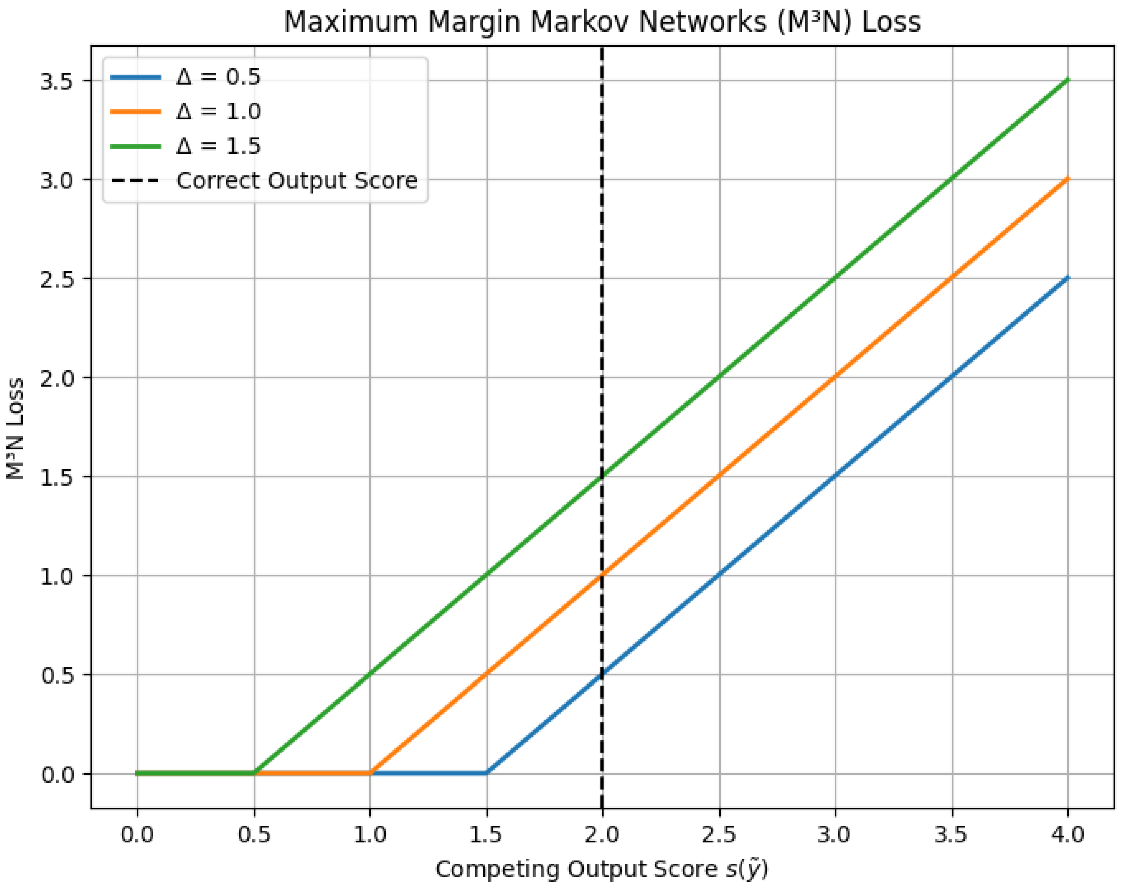
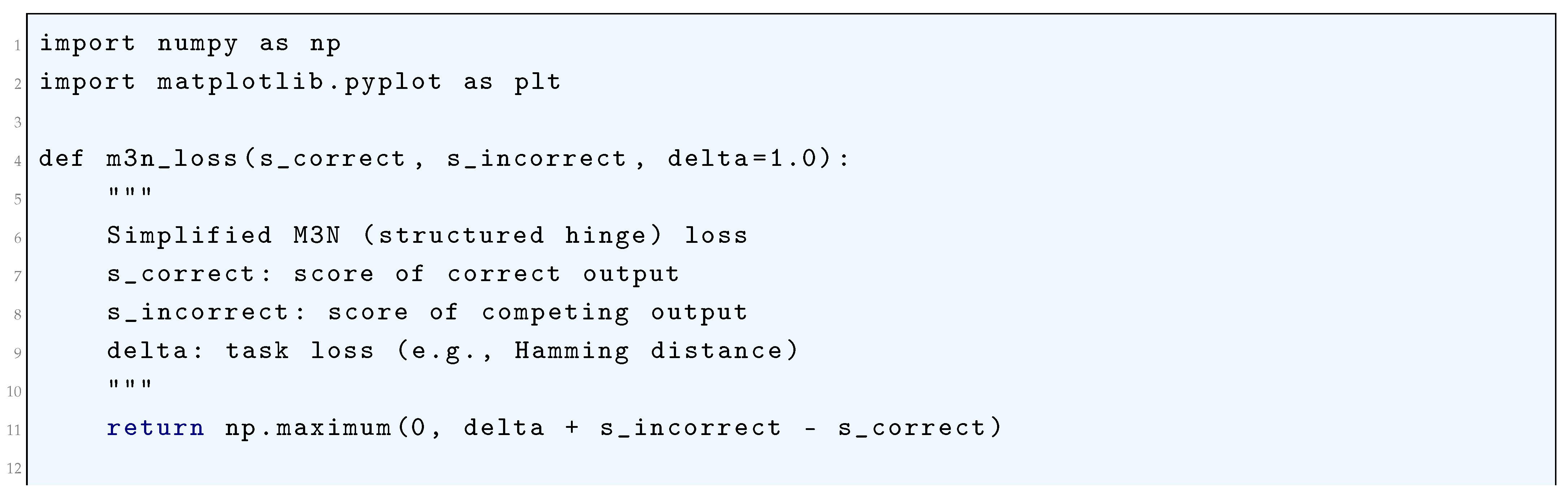
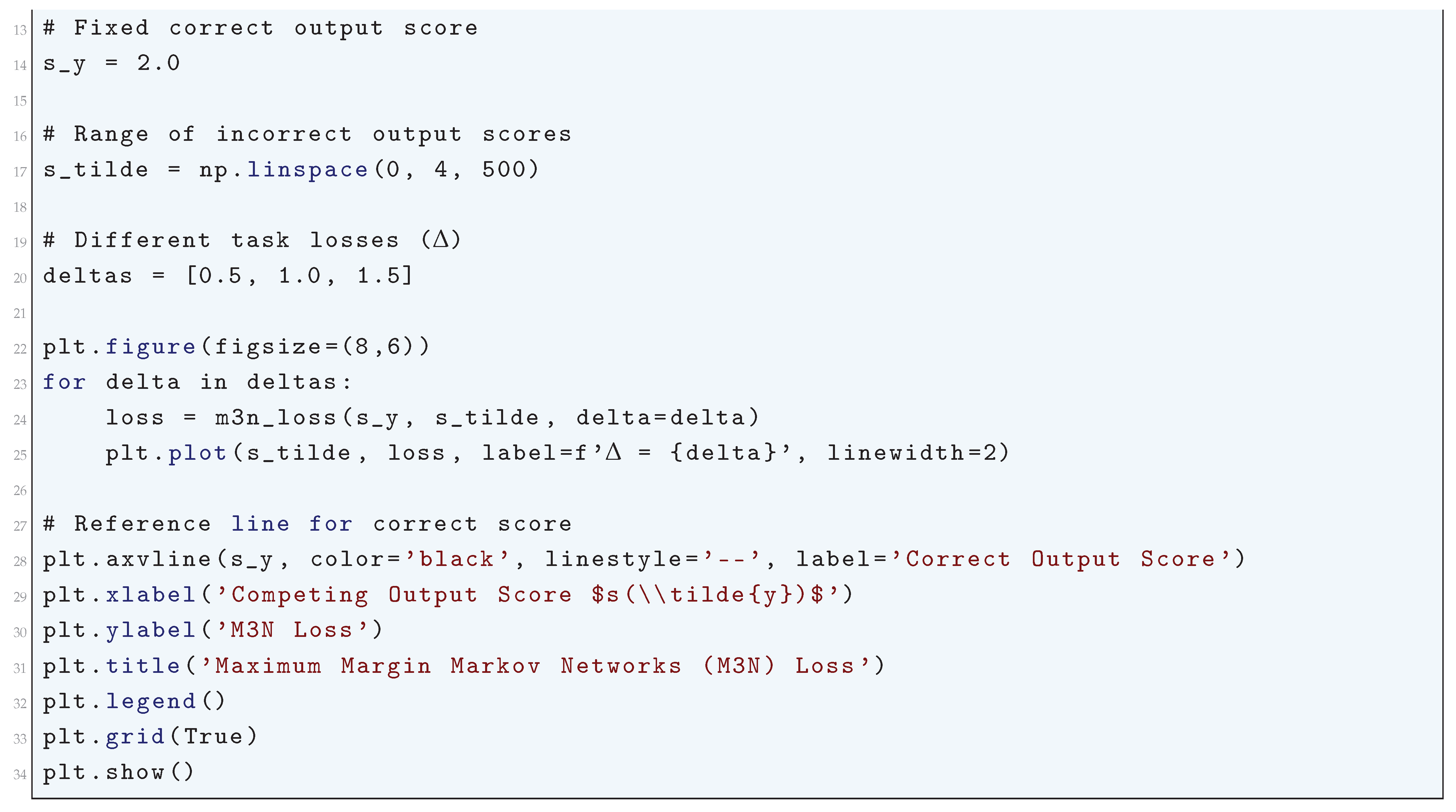
10.5.3.62 Python Code to Generate Figure 129 Illustrating M³N Loss Surface ()
The Python code below produces the Figure 129 illustrating M³N Loss Surface ().
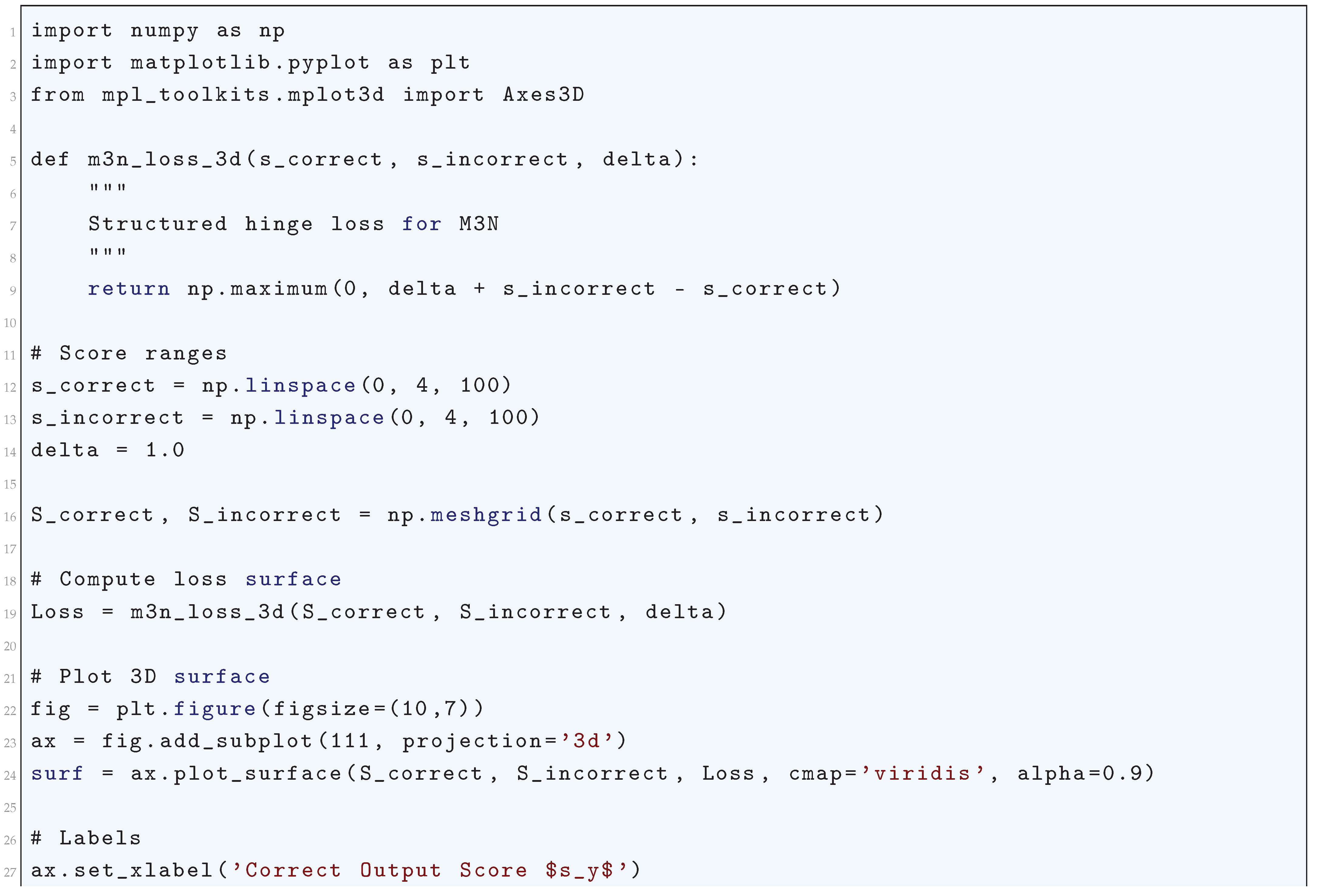
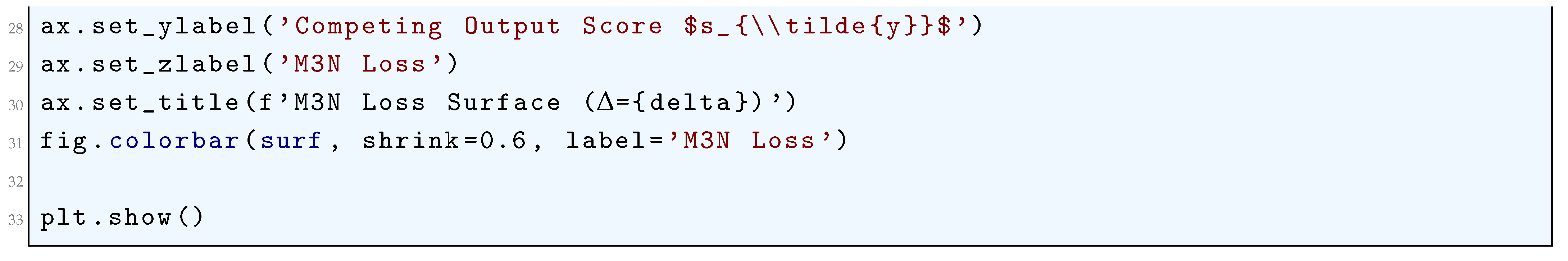
Figure 129.
M³N Loss Surface ()
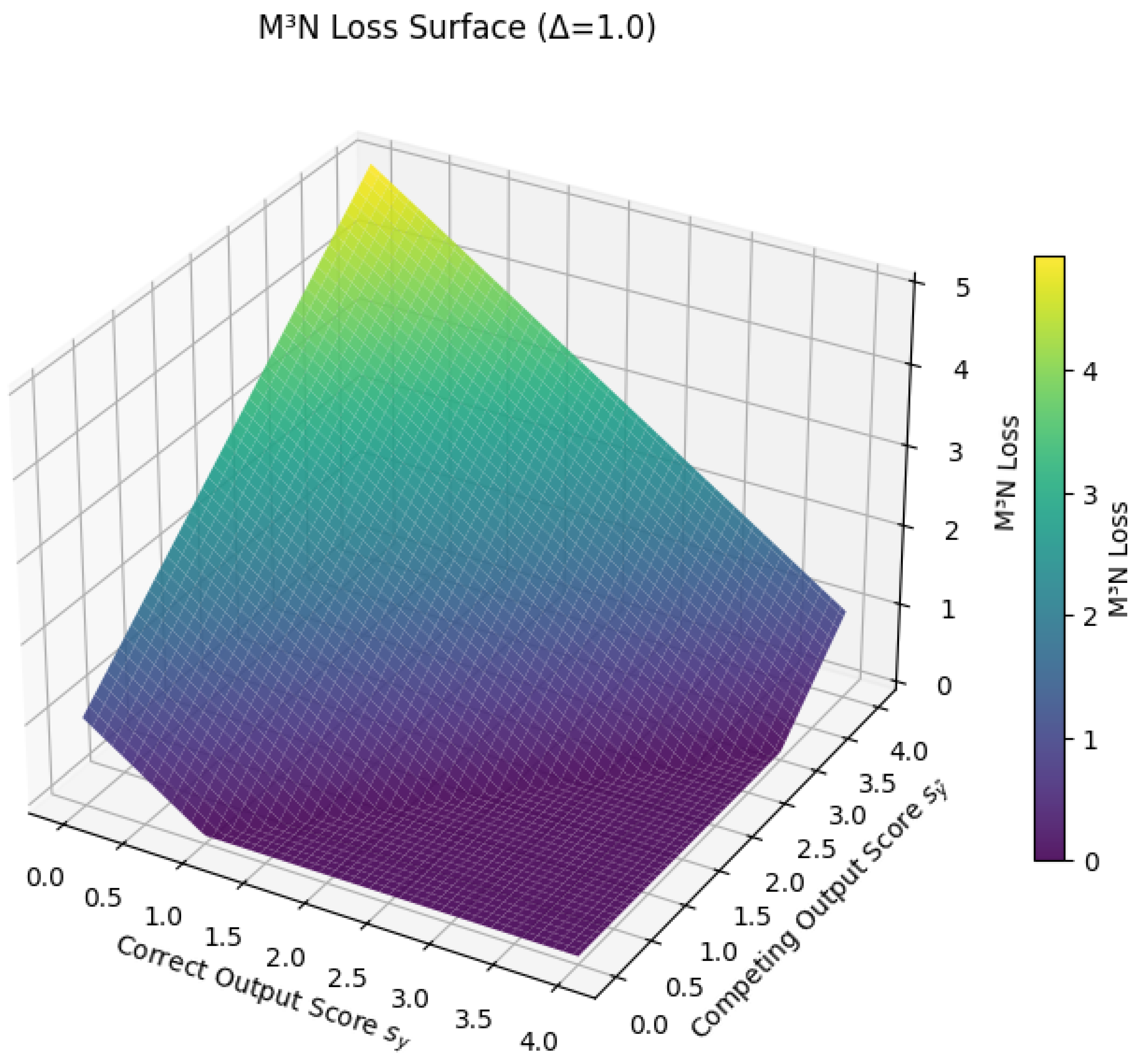
10.5.3.63 Python Code to Generate Figure 130 Illustrating Contour Plot of M³N Loss ()
The Python code below produces the Figure 130 illustrating Contour Plot of M³N Loss ().
Figure 130.
Contour Plot of M³N Loss ()
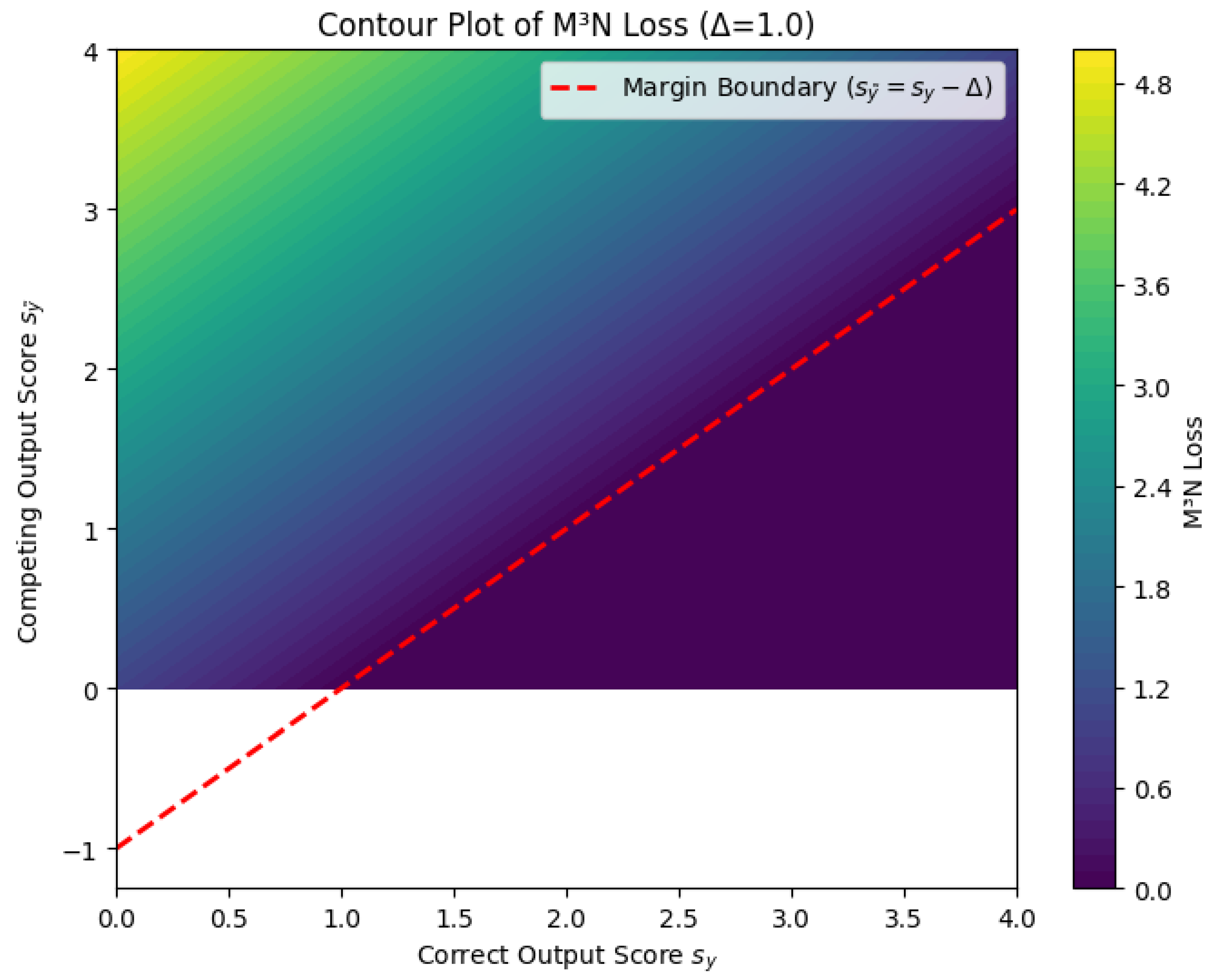
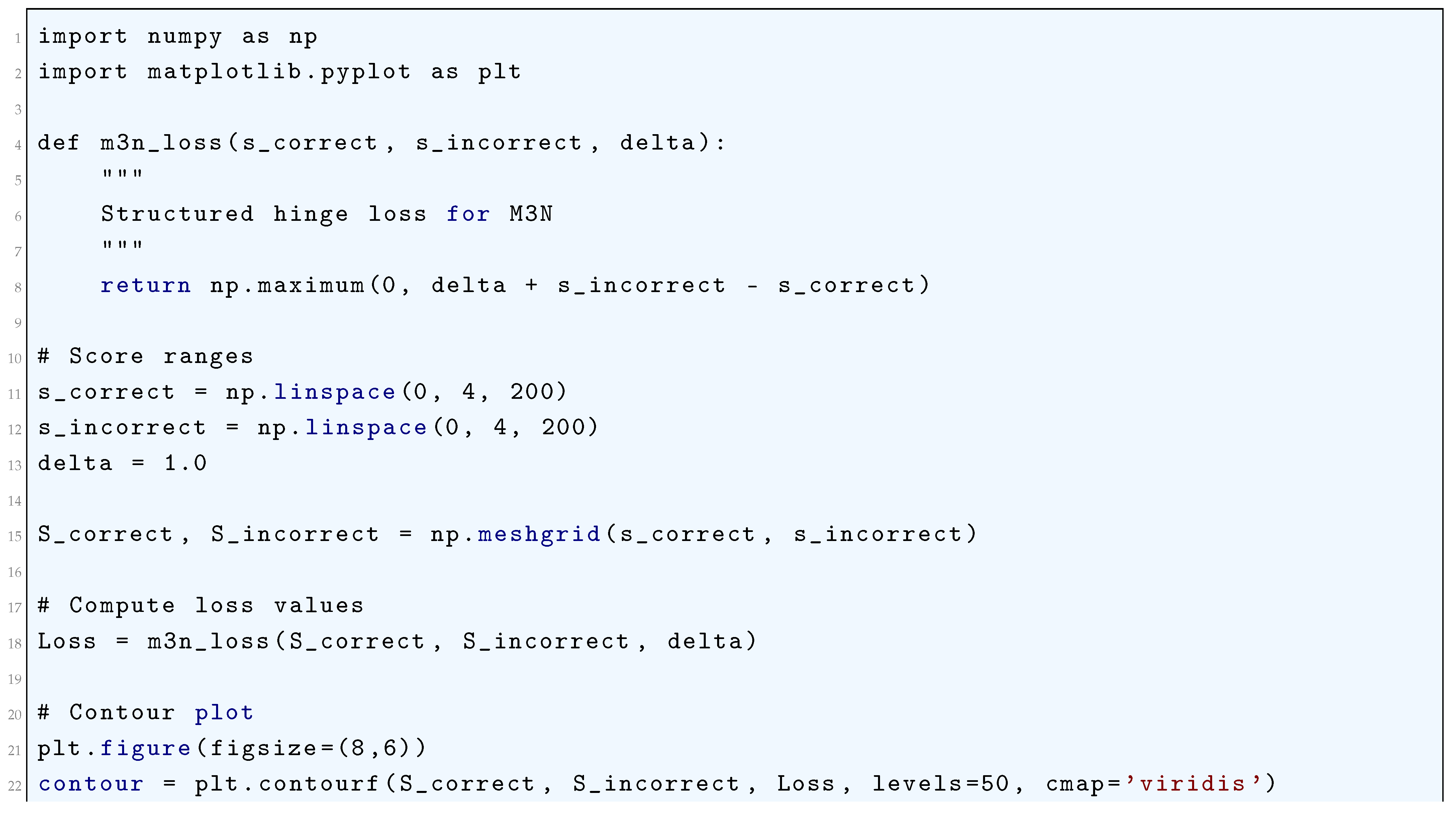
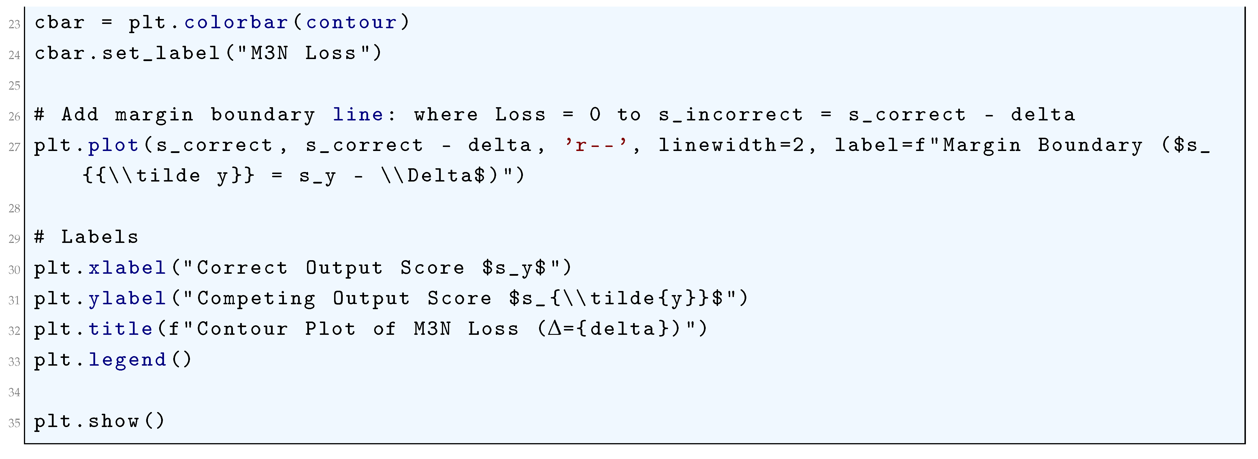
10.5.3.64 Python Code to Generate Figure 131 Illustrating Listwise Ranking Losses (ListNet vs ListMLE)
The Python code below produces the Figure 131 illustrating Listwise Ranking Losses (ListNet vs ListMLE).
Figure 131.
Listwise Ranking Losses (ListNet vs ListMLE)
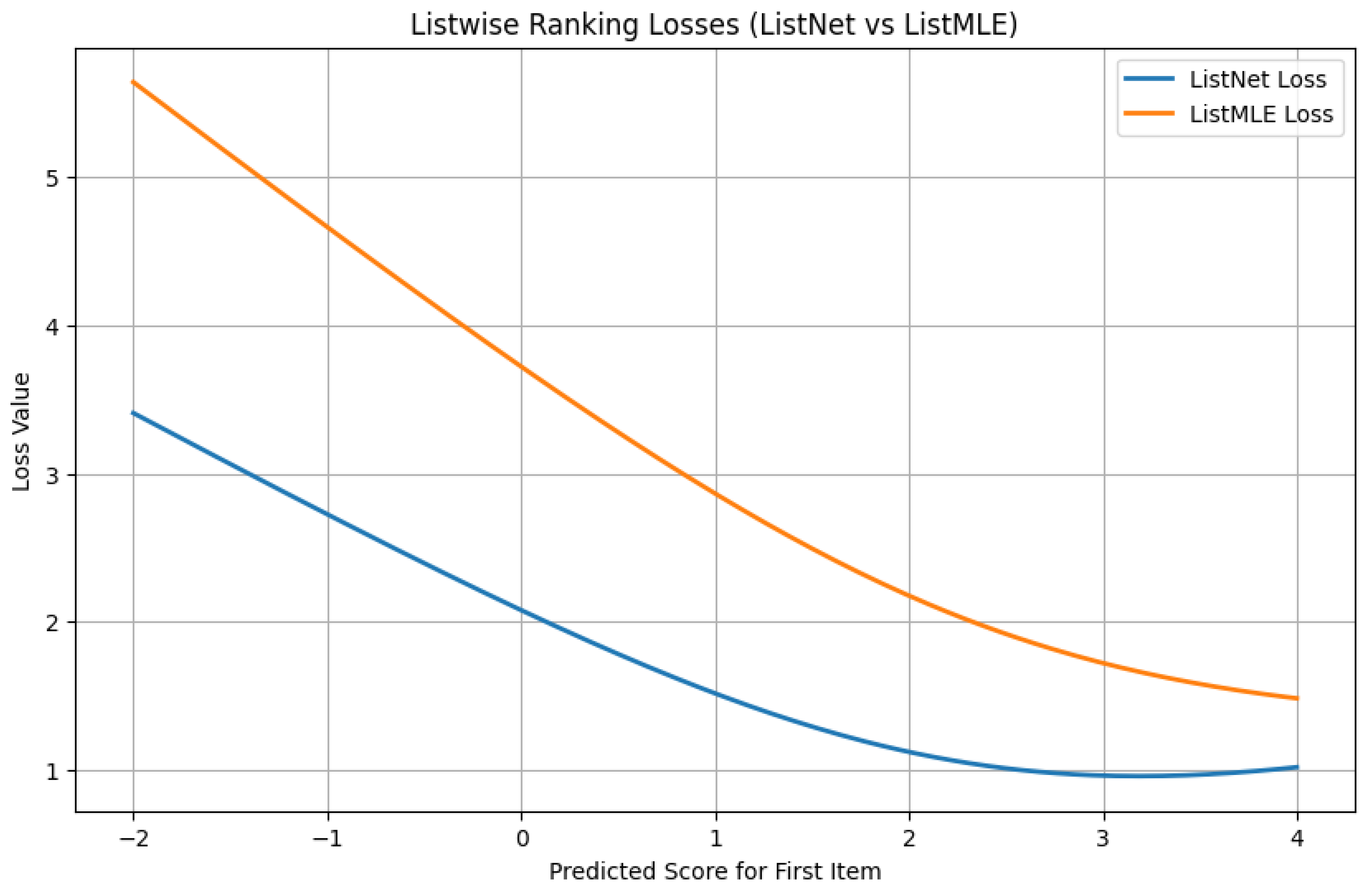
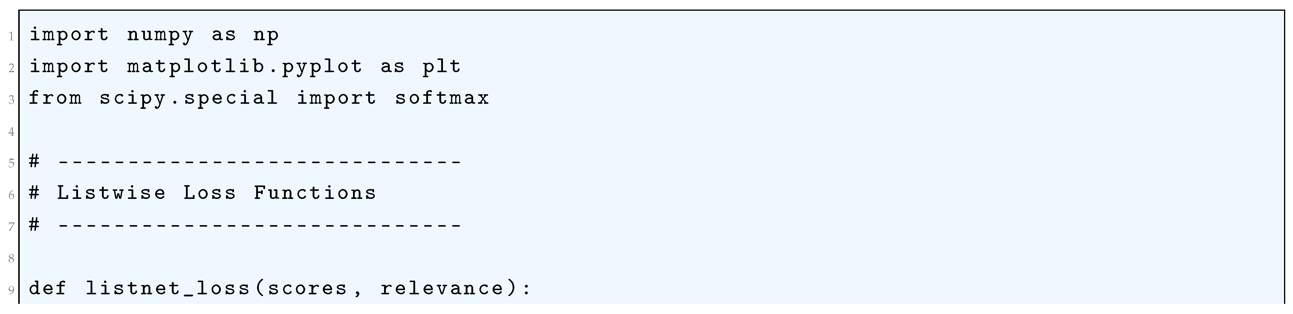
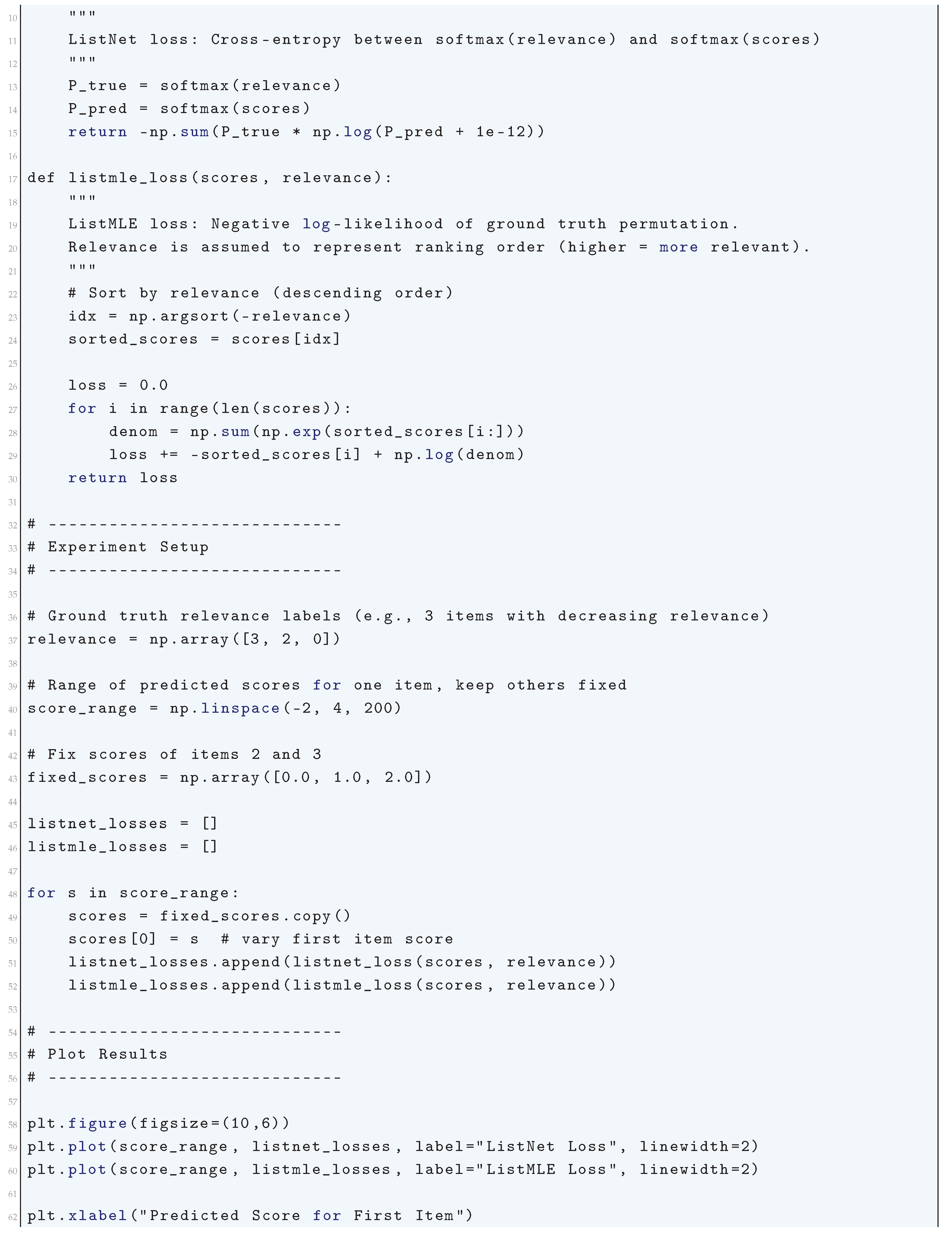
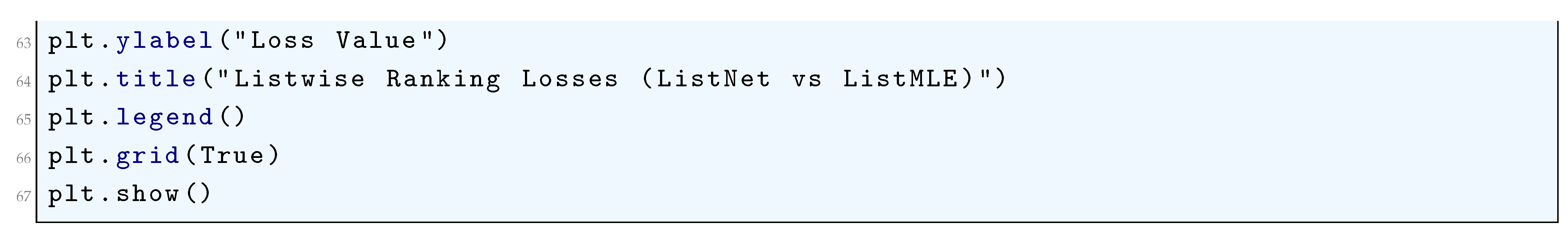
10.5.3.65 Python Code to Generate Figure 132 Illustrating Listwise Ranking Losses (3D Surfaces)
The Python code below produces the Figure 132 illustrating Listwise Ranking Losses (3D Surfaces).
Figure 132.
Listwise Ranking Losses (3D Surfaces)
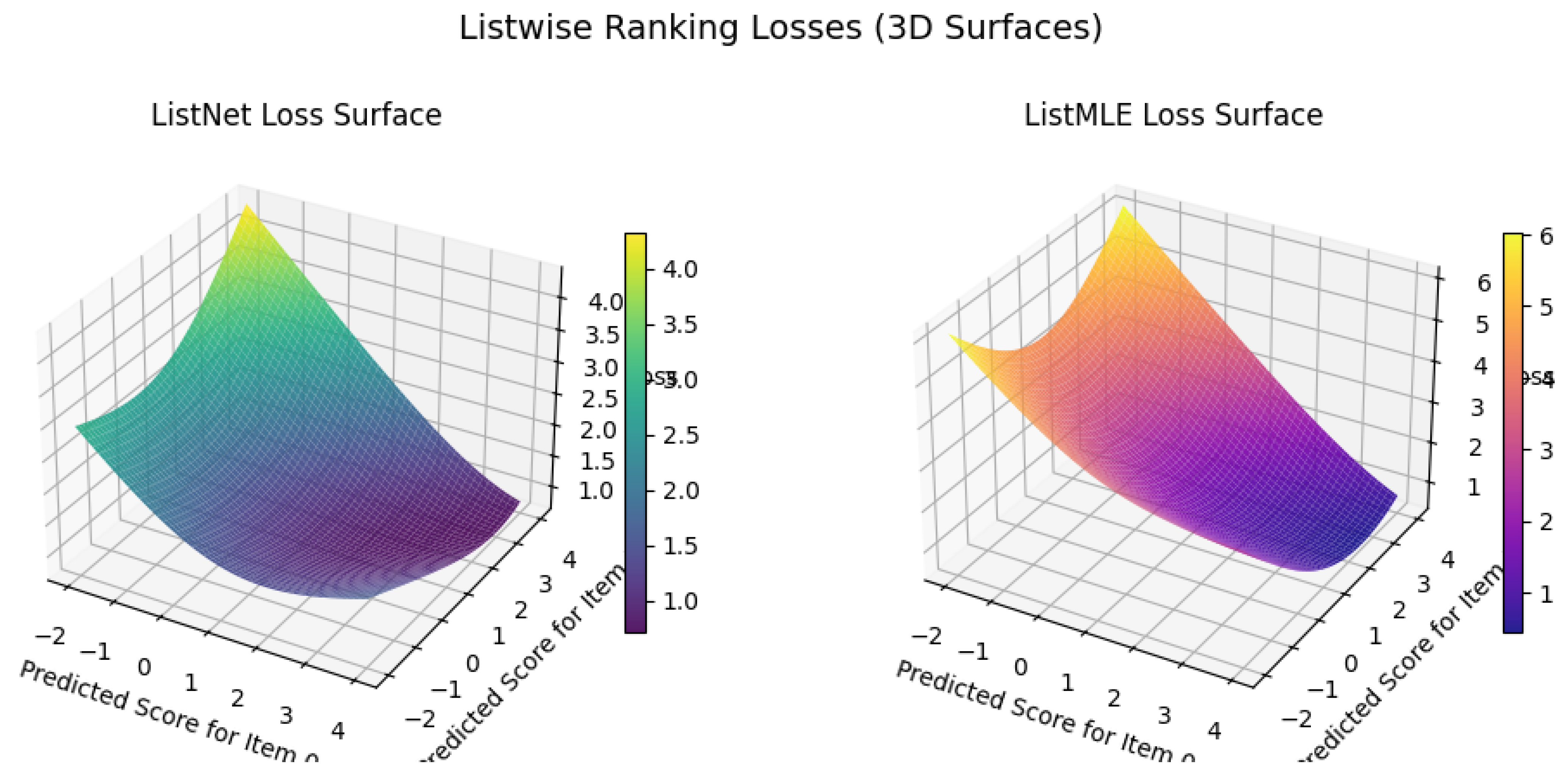
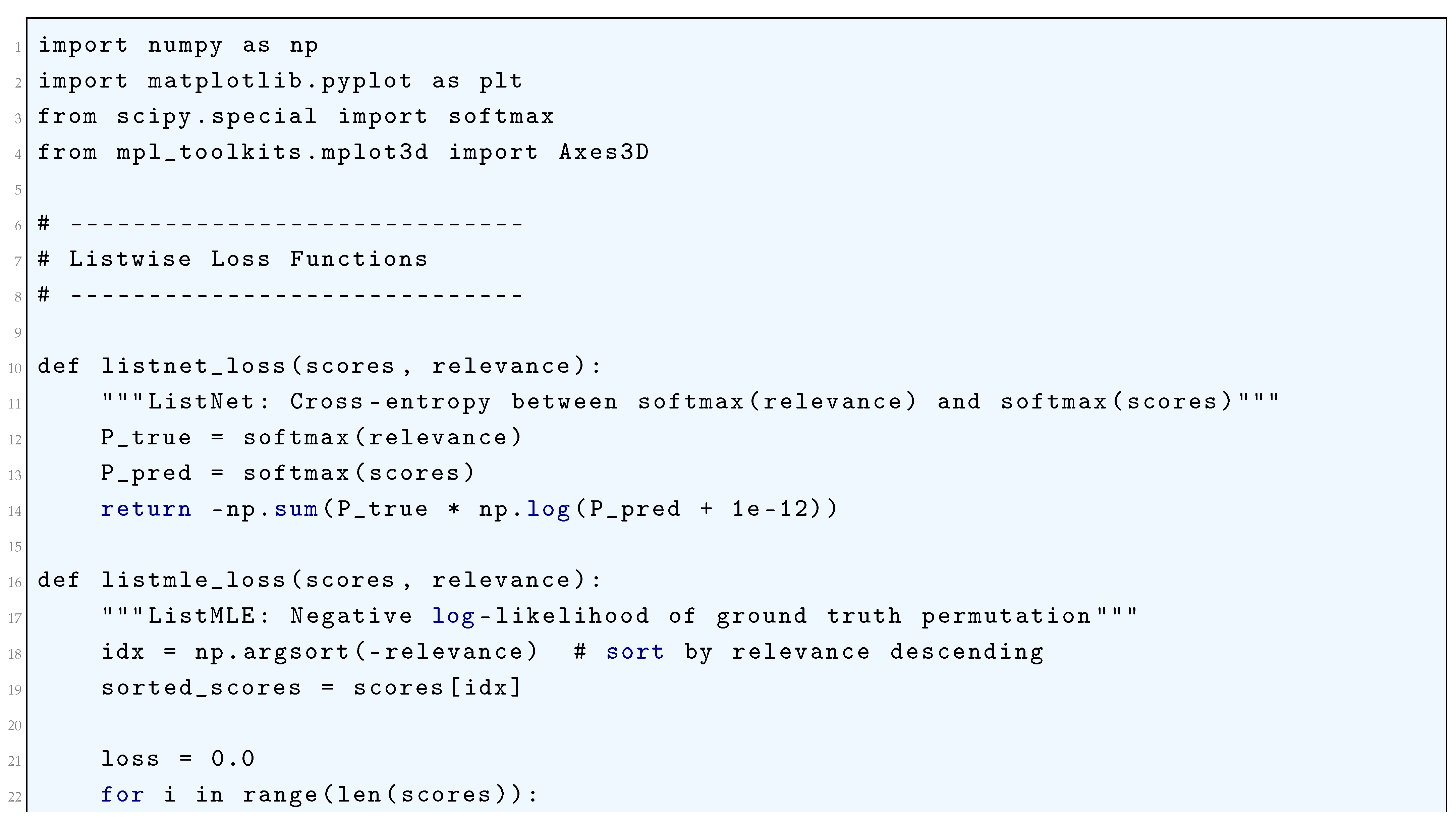
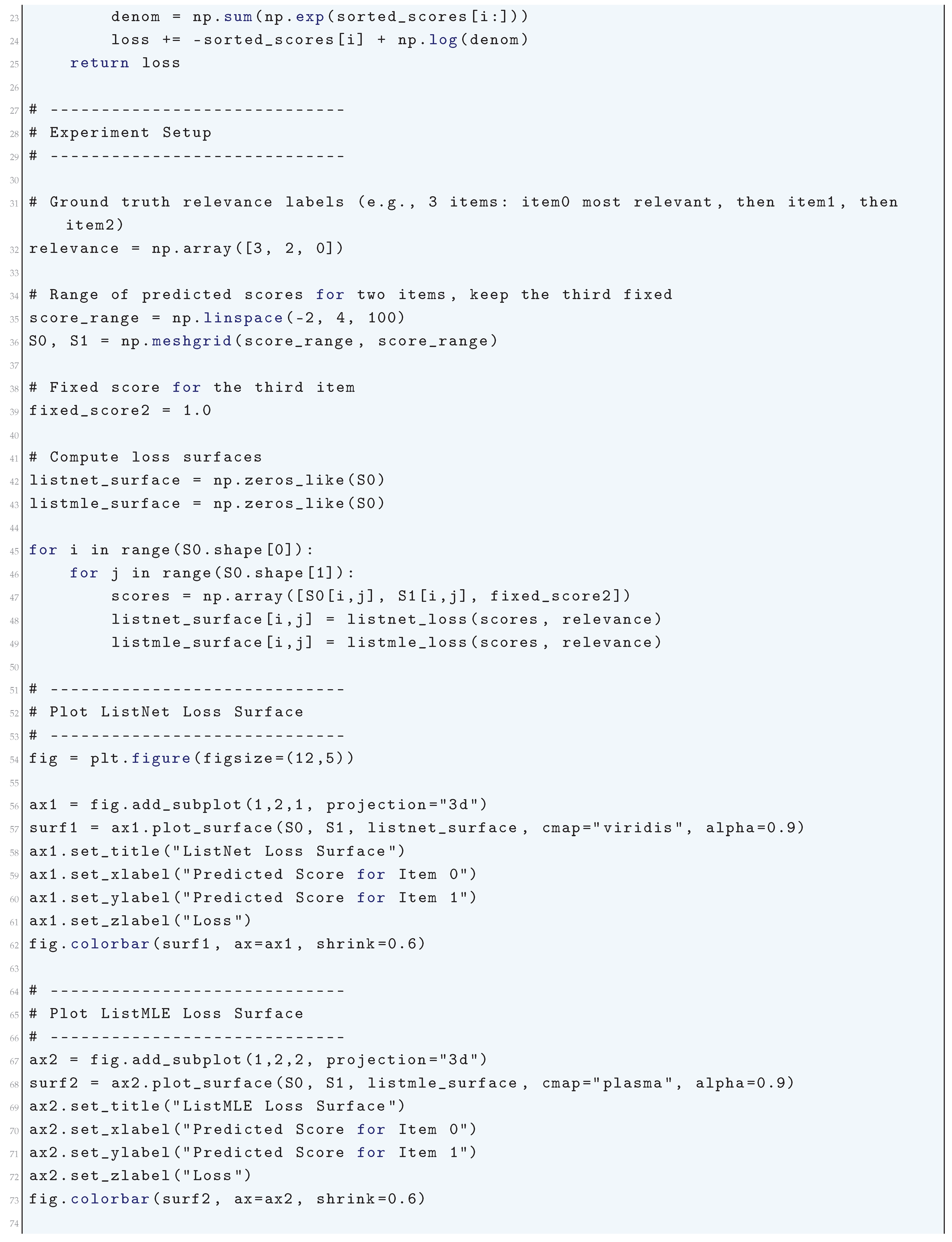

10.5.3.66 Python Code to Generate Figure 133 Illustrating Listwise Ranking Loss Contours
The Python code below produces the Figure 133 illustrating Listwise Ranking Loss Contours.
Figure 133.
Listwise Ranking Loss Contours
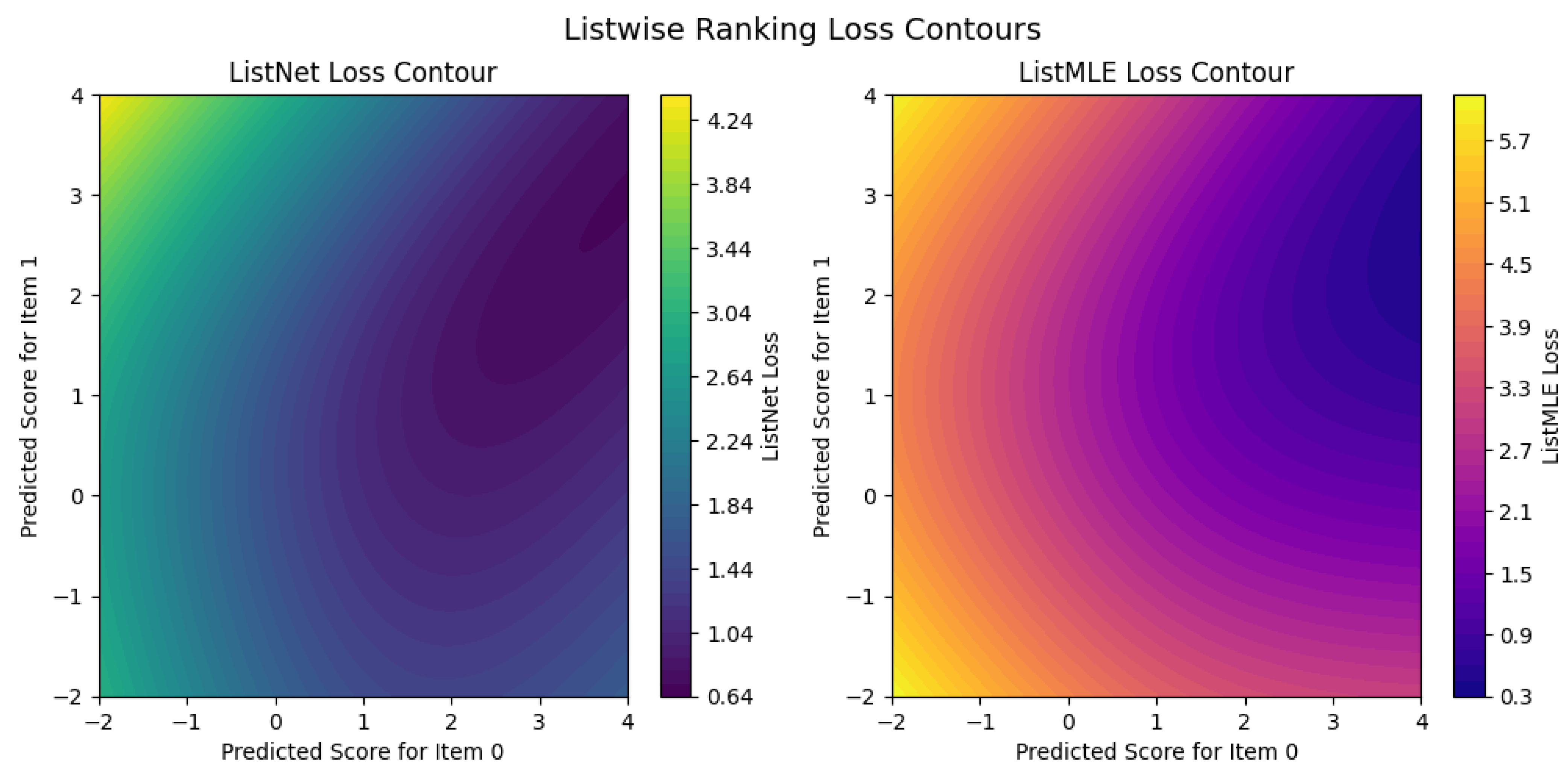
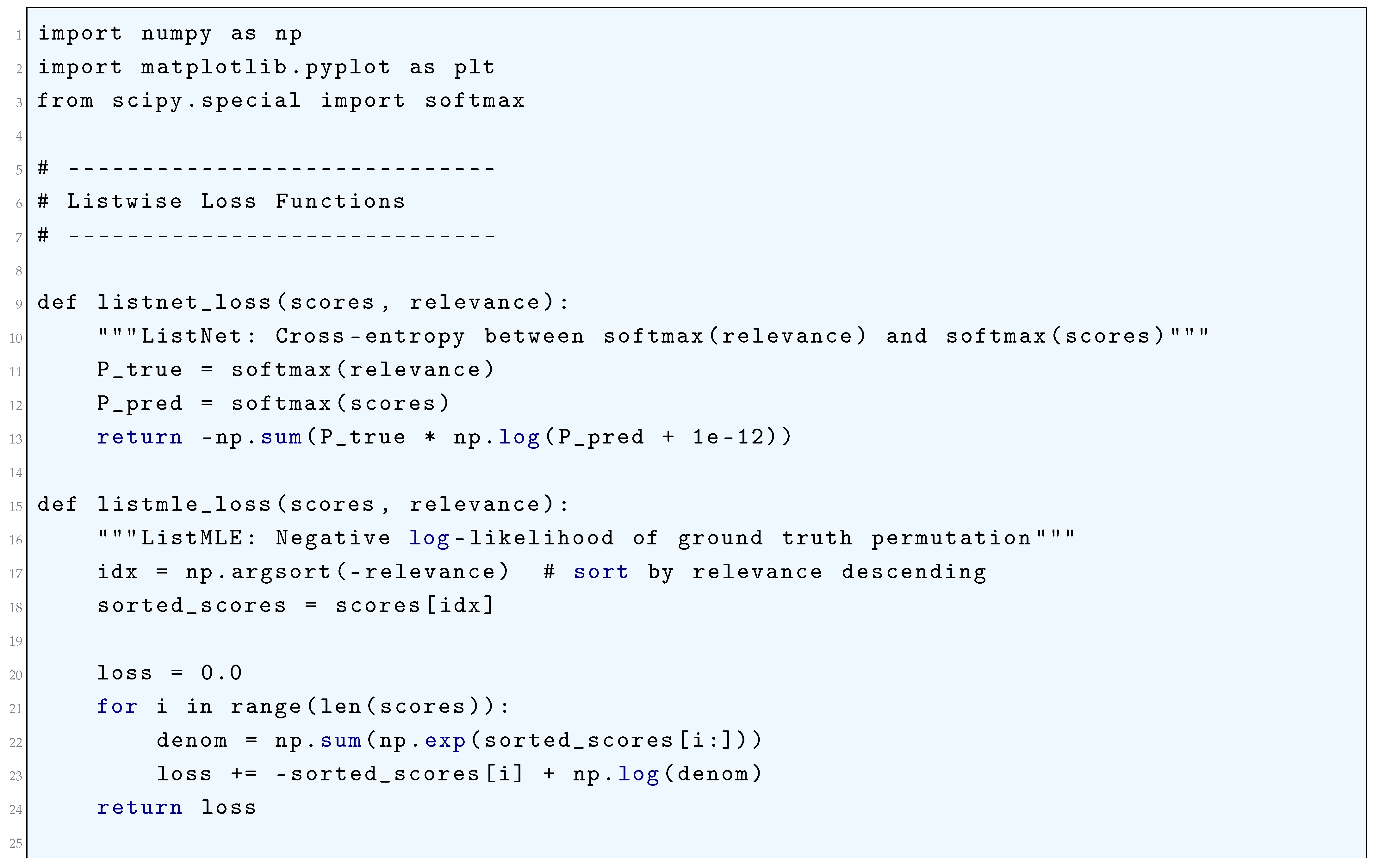
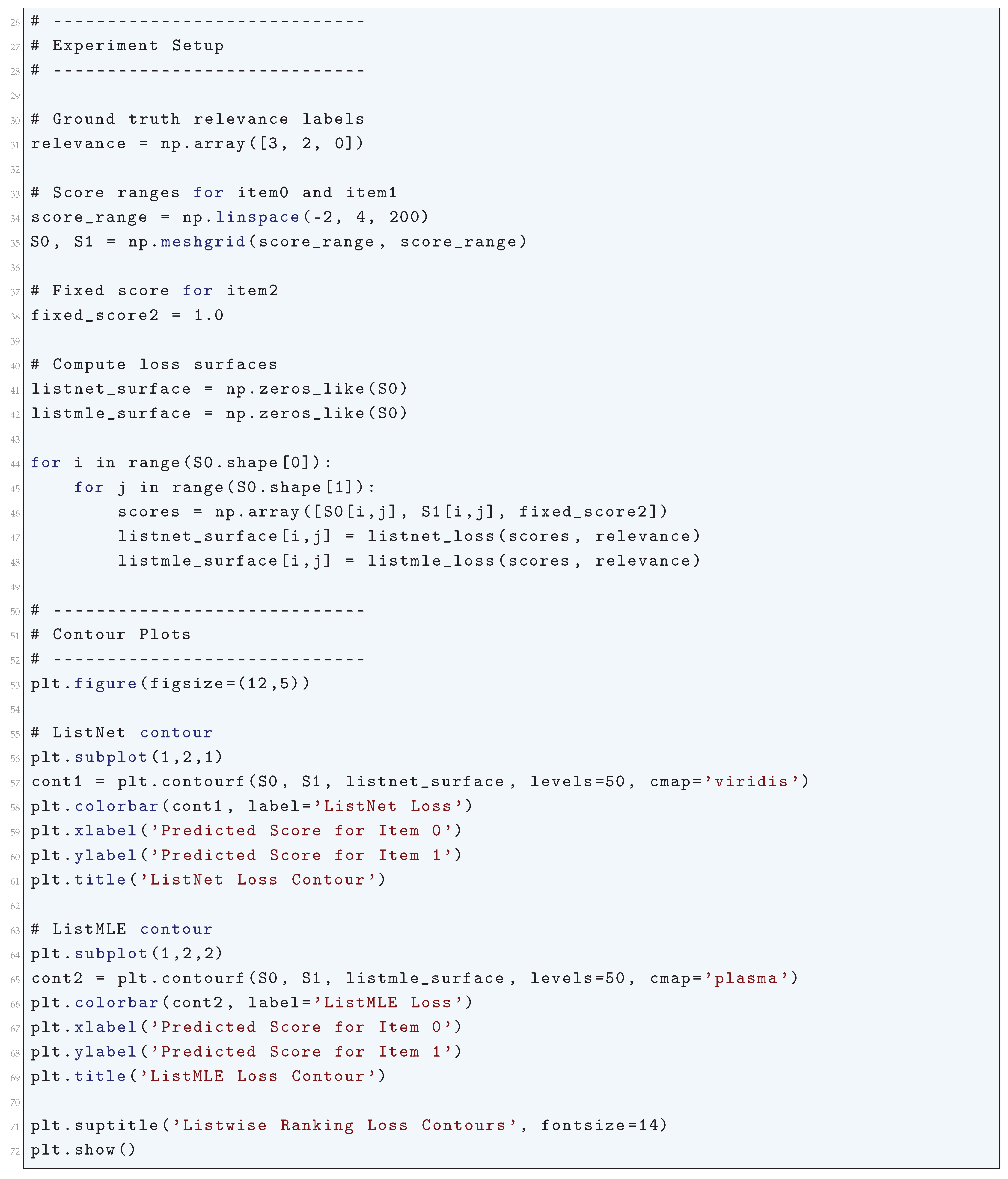
10.5.3.67 Python Code to Generate Figure 134 illustrating Pairwise Ranking Losses
The Python code below produces the Figure 134 illustrating Pairwise Ranking Losses.
Figure 134.
Pairwise Ranking Losses
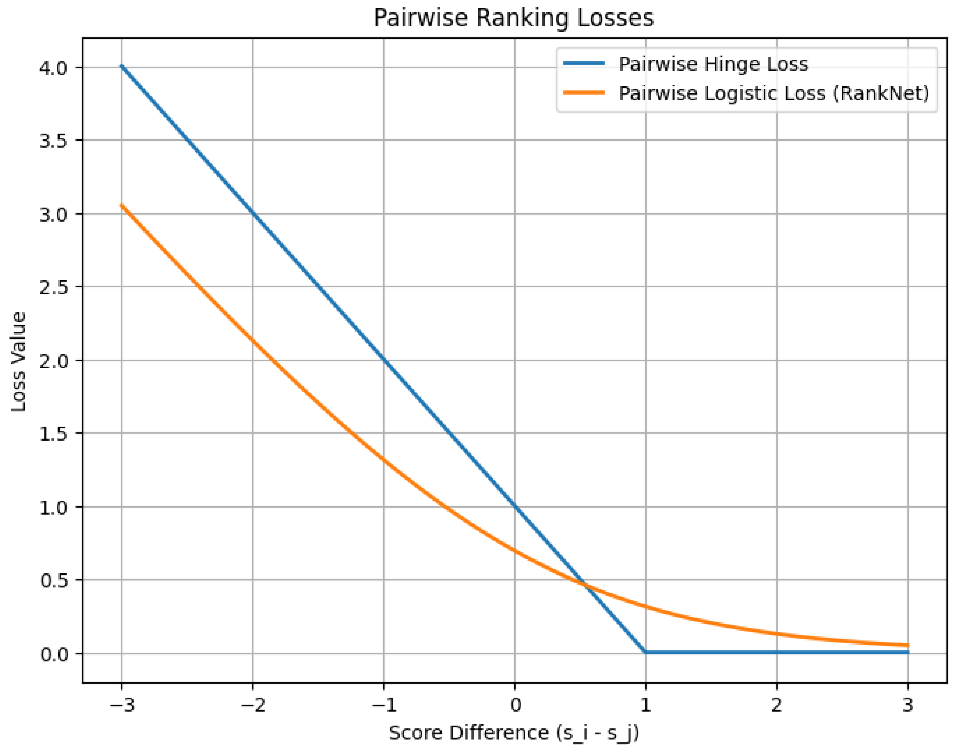
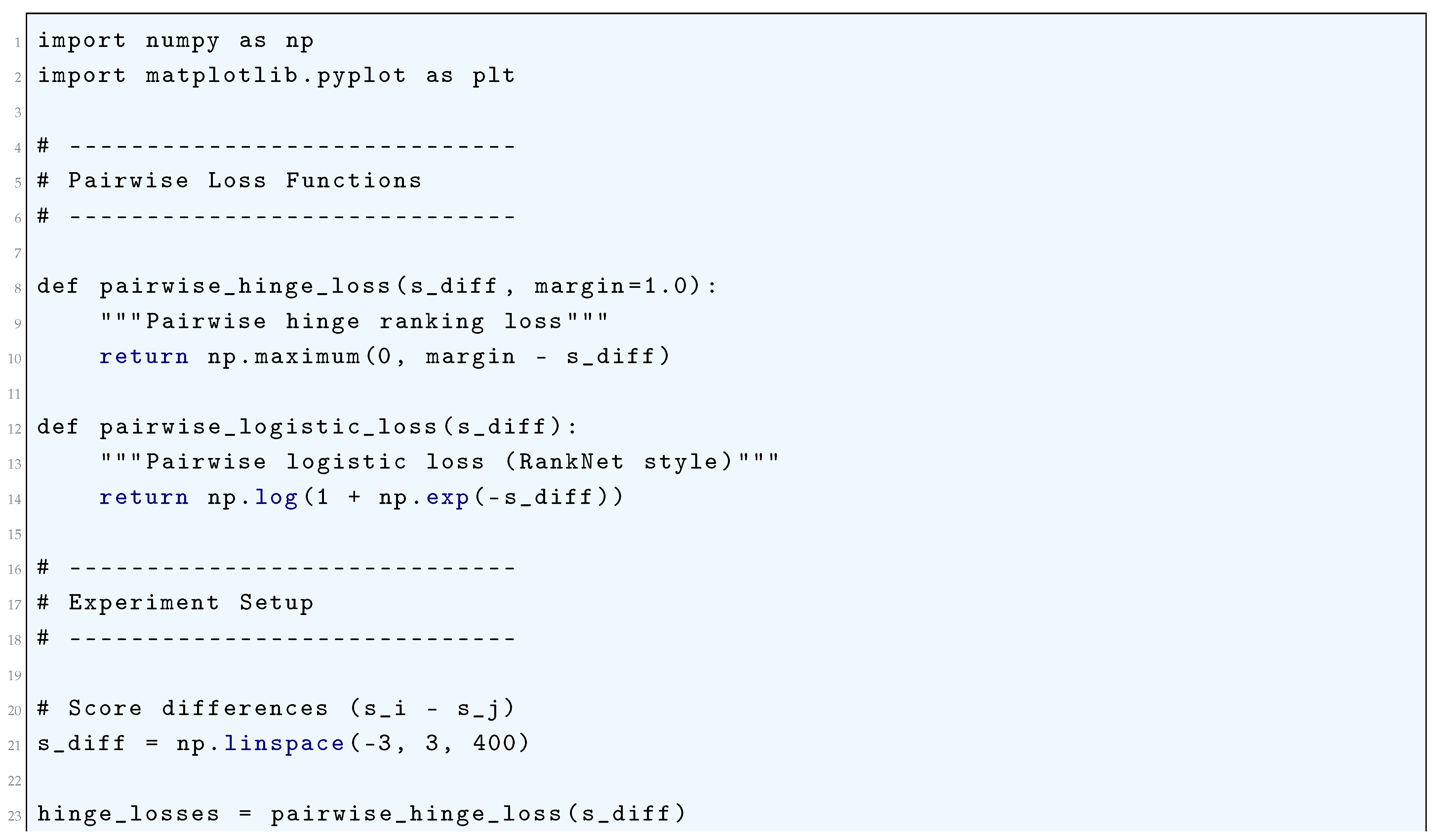
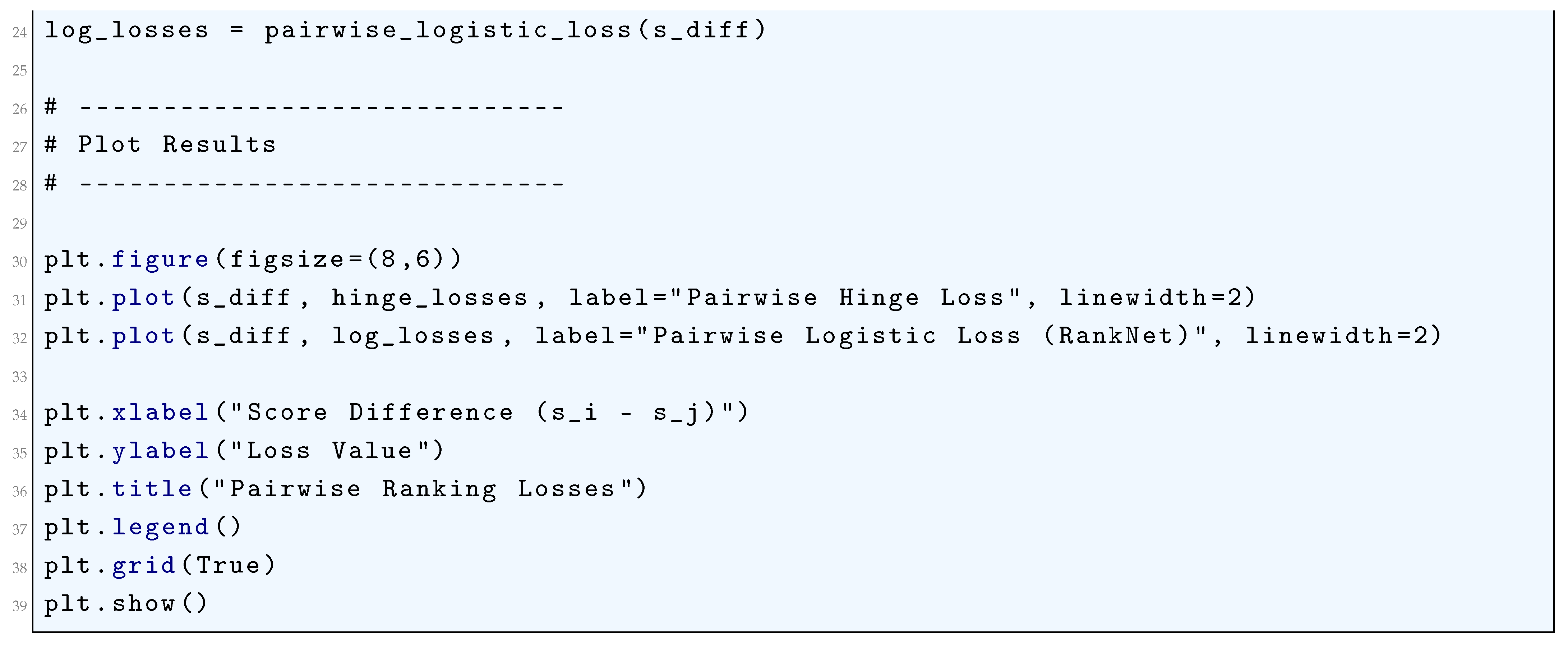
10.5.3.68 Python Code to Generate Figure 135 Illustrating Pairwise Ranking Loss Landscapes
The Python code below produces the Figure 135 illustrating Pairwise Ranking Loss Landscapes.
Figure 135.
Pairwise Ranking Loss Landscapes
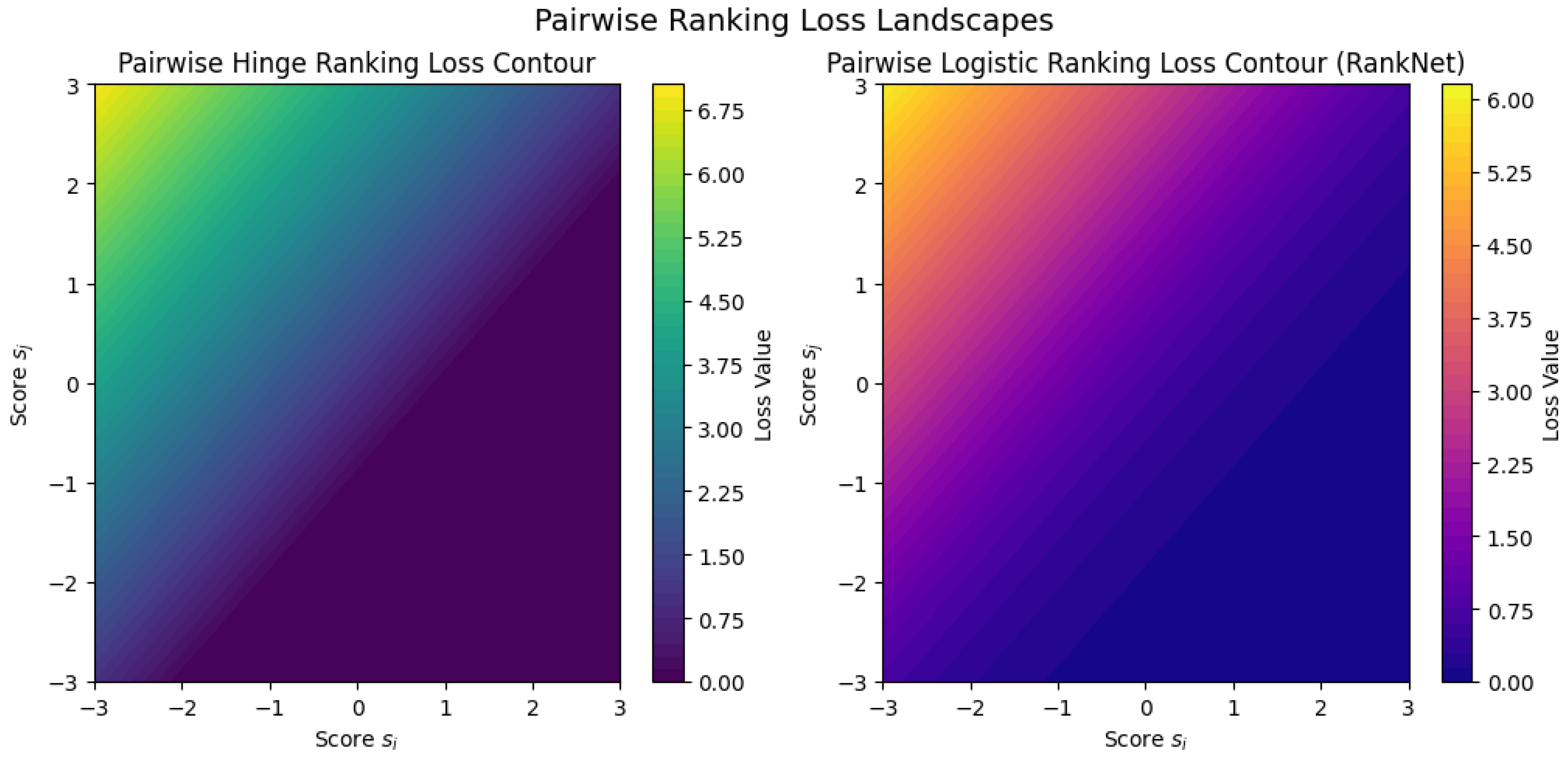
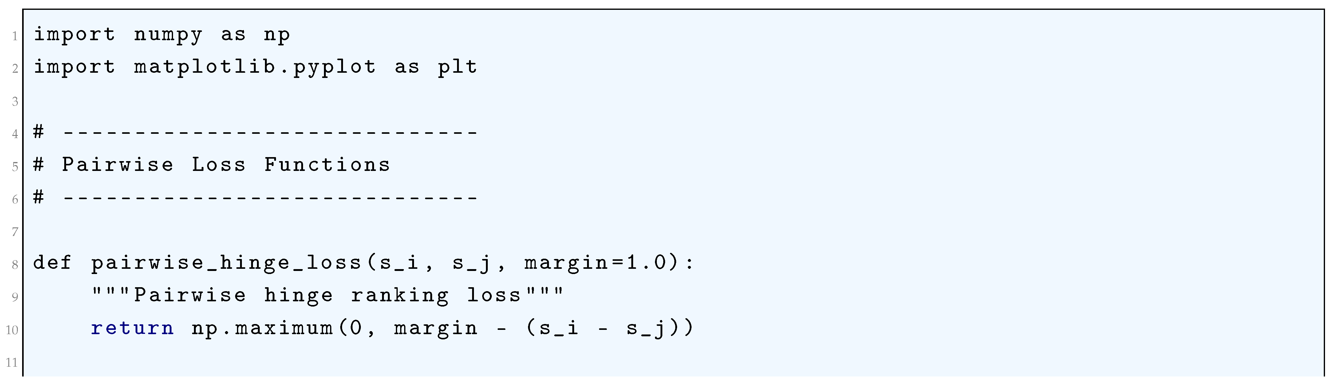

10.5.3.69 Python Code to Generate Figure 136 Illustrating 3D Surfaces of Pairwise Ranking Losses
The Python code below produces the Figure 136 illustrating 3D Surfaces of Pairwise Ranking Losses.
Figure 136.
3D Surfaces of Pairwise Ranking Losses
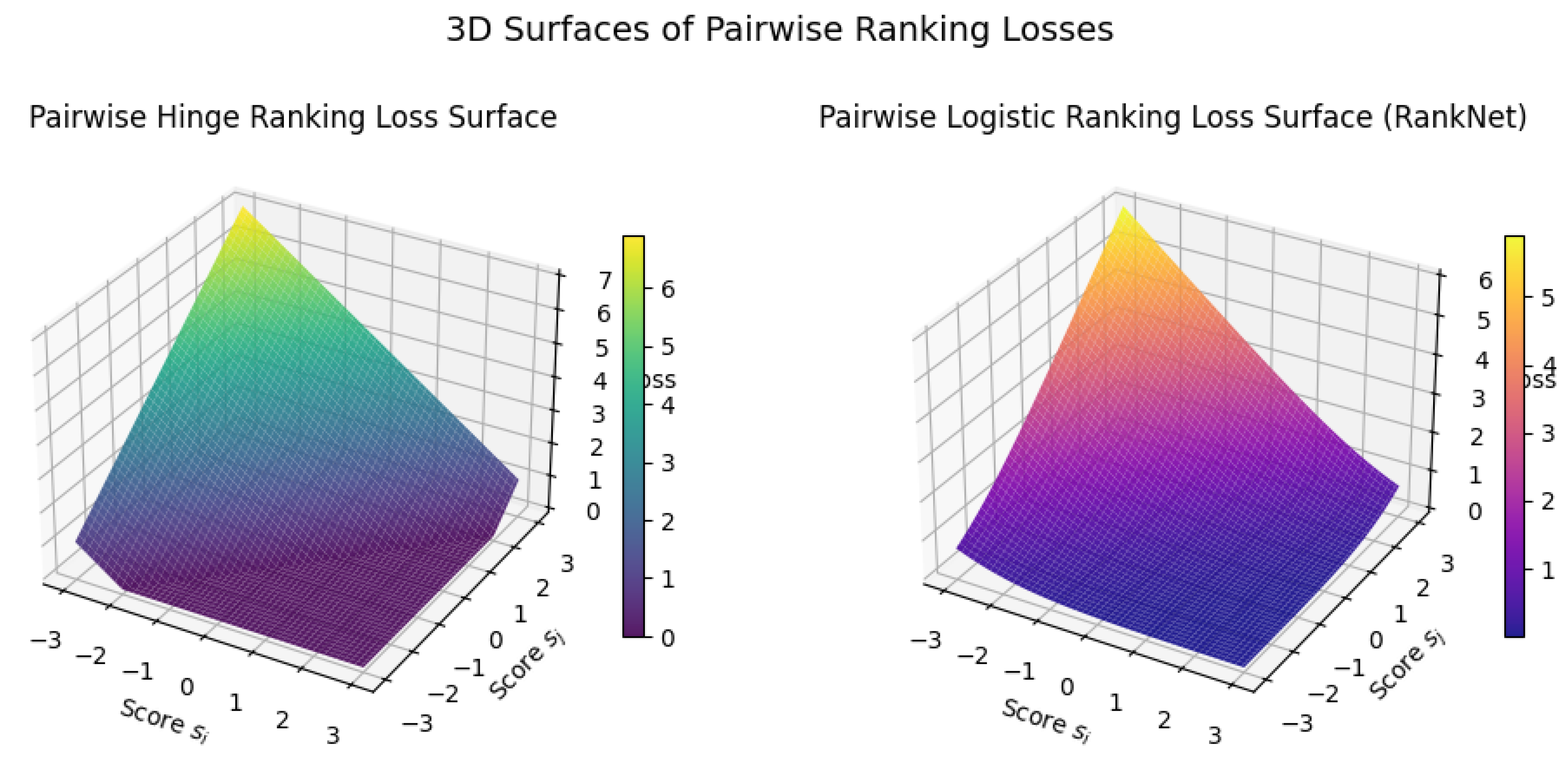
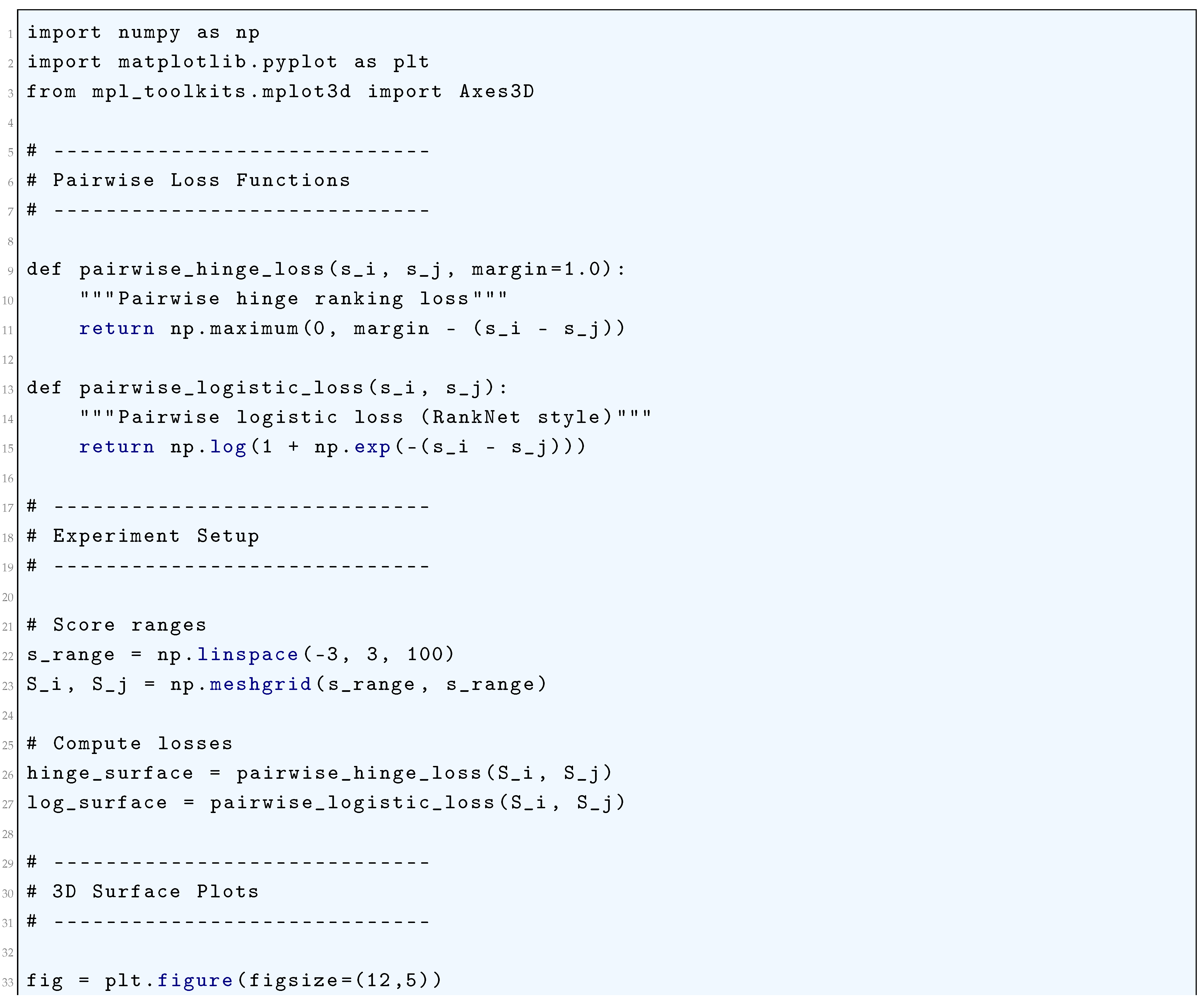
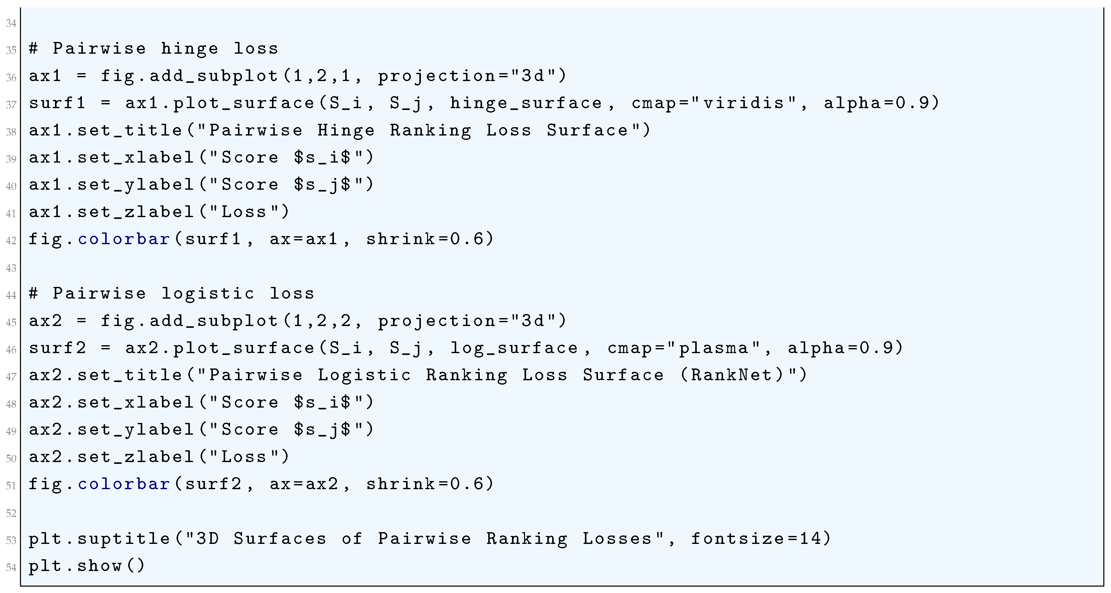
10.5.3.70 Python Code to Generate Figure 137 Illustrating Contrastive Divergence (CD) Loss vs Weight
The Python code below produces the Figure 137 illustrating Contrastive Divergence (CD) Loss vs Weight.
Figure 137.
Contrastive Divergence (CD) Loss vs Weight
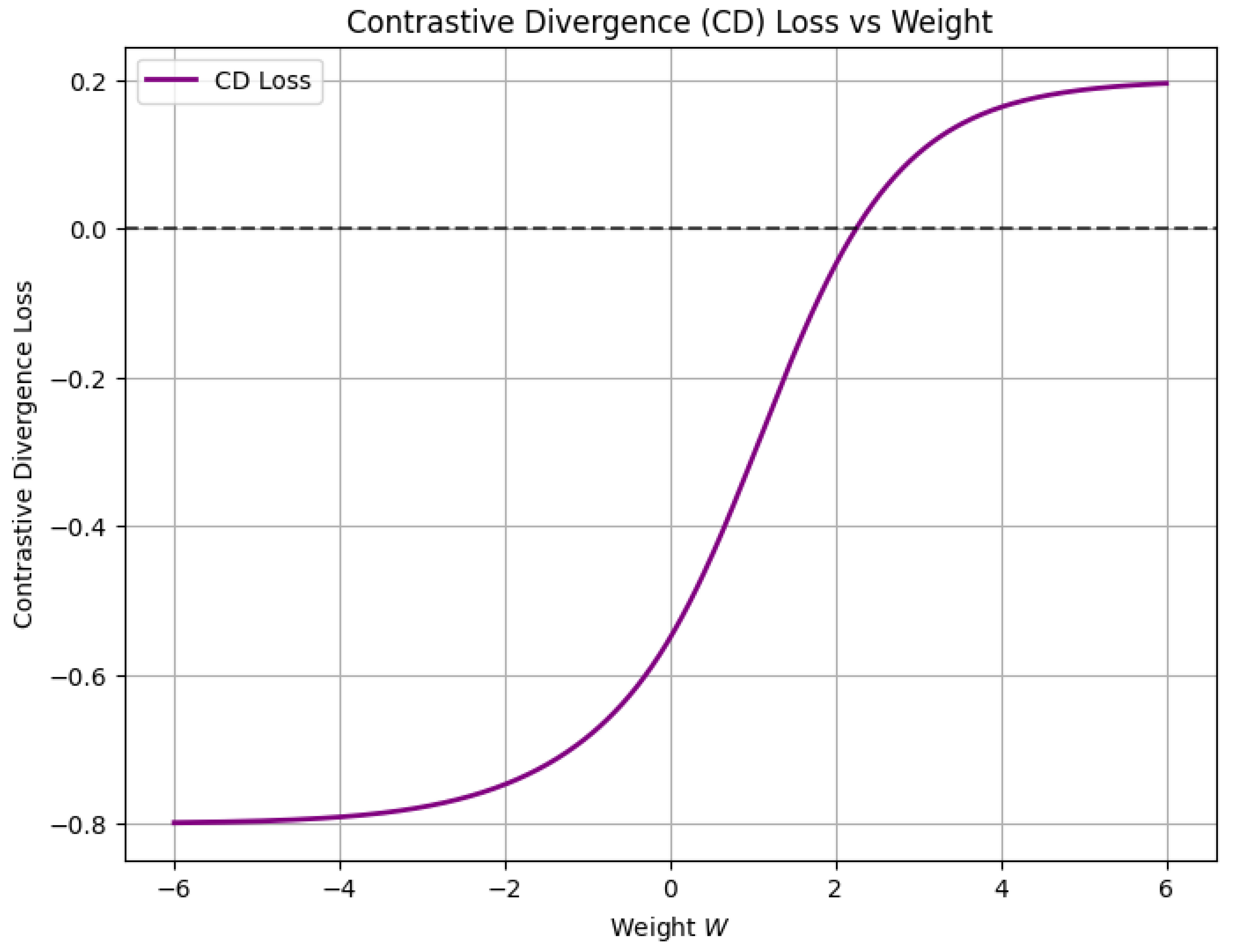
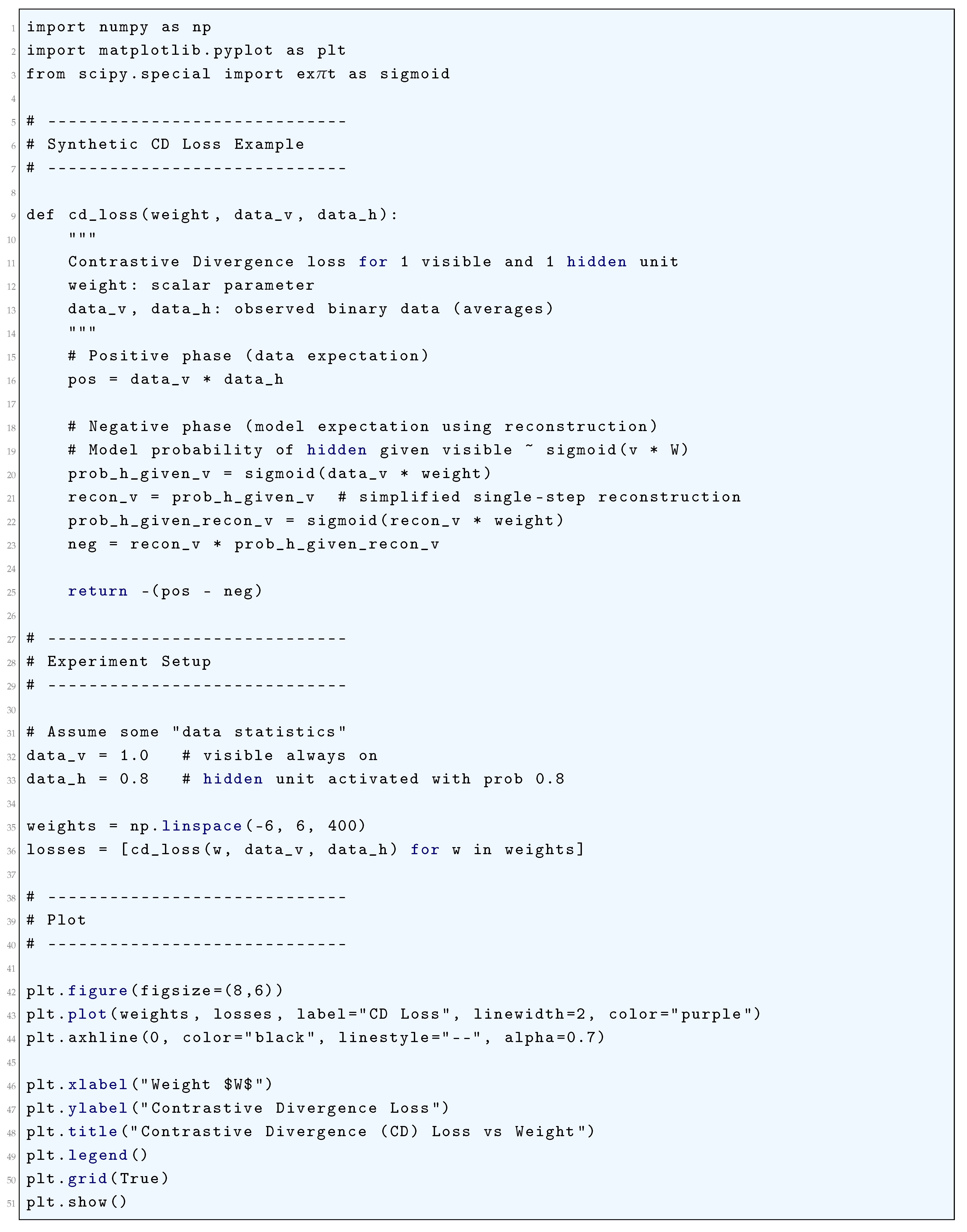
10.5.3.71 Python Code to Generate Figure 138 Illustrating Contrastive Divergence (CD) Loss Landscape
The Python code below produces the Figure 138 illustrating Contrastive Divergence (CD) Loss Landscape.
Figure 138.
Contrastive Divergence (CD) Loss Landscape
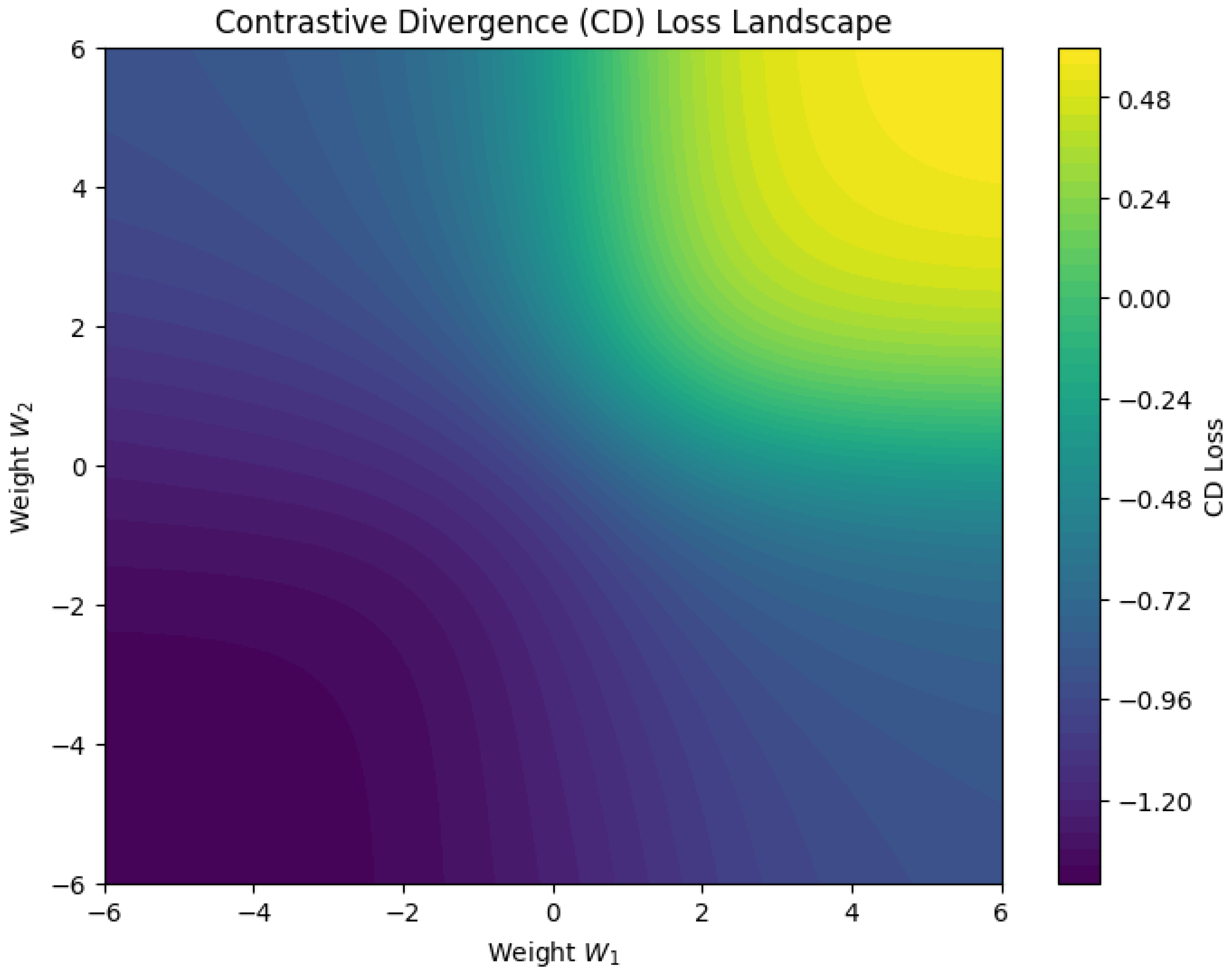
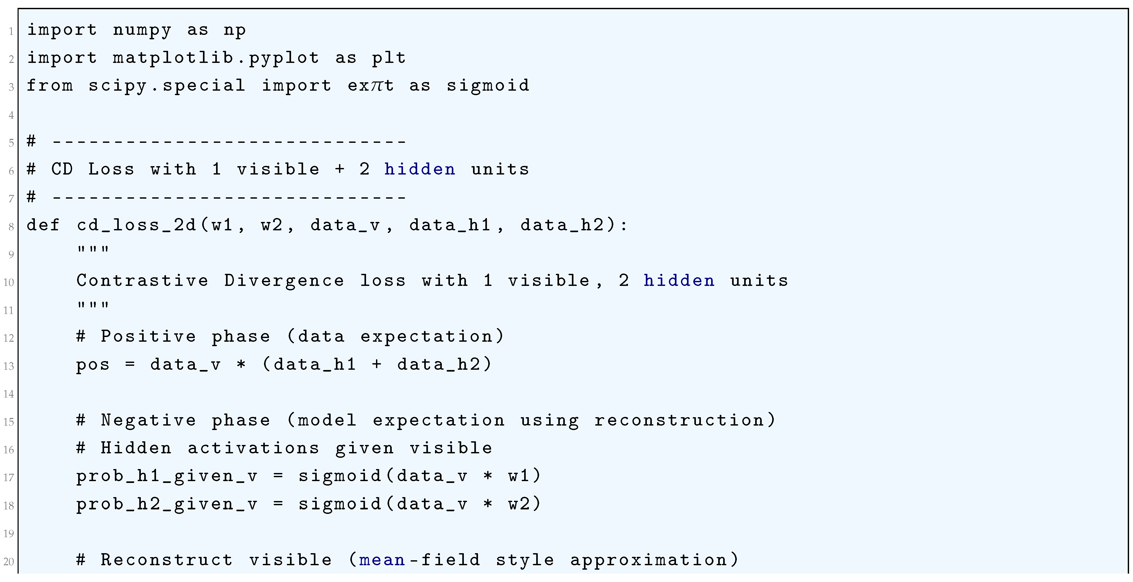
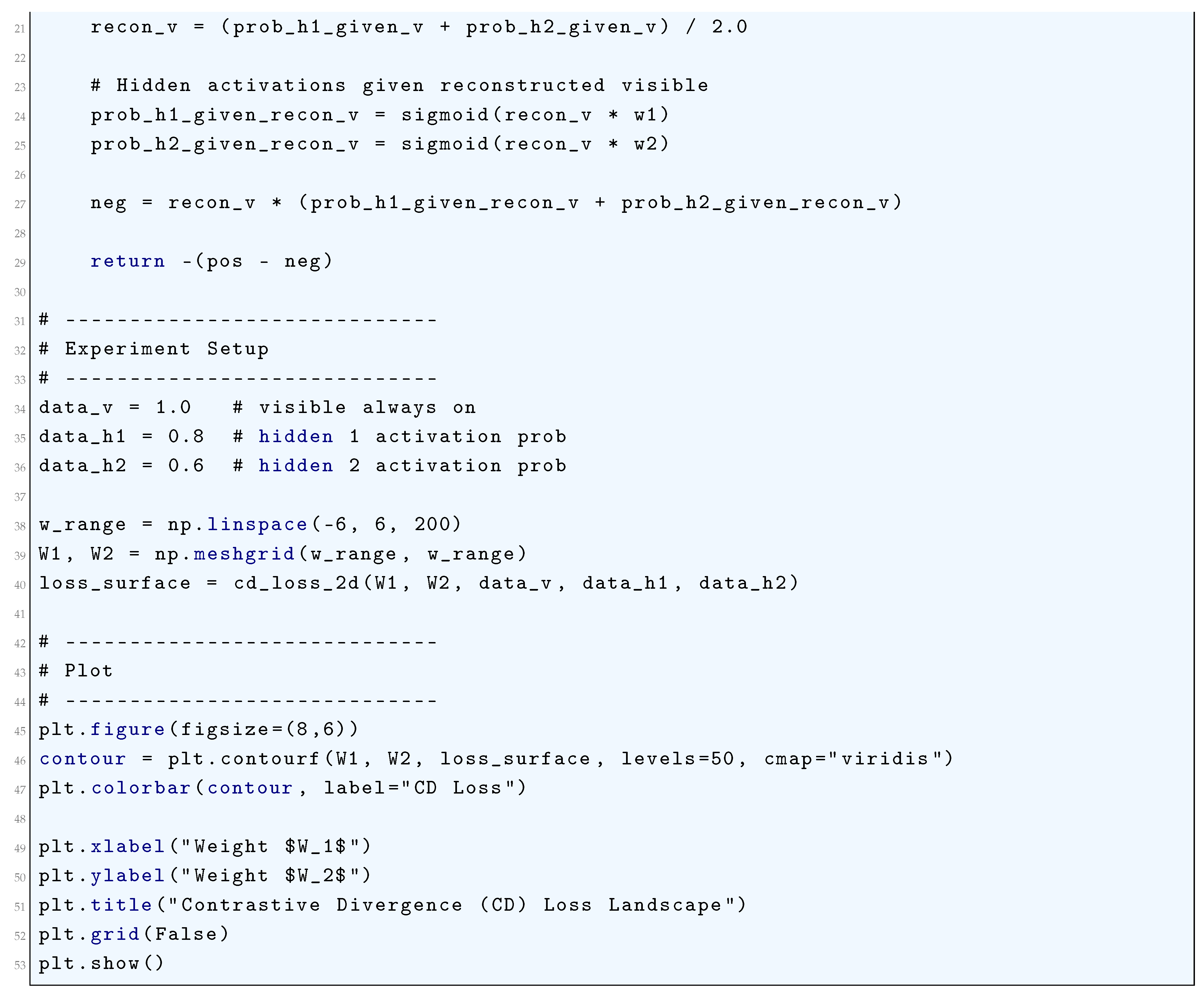
10.5.3.72 Python Code to Generate Figure 139 Illustrating Contrastive Divergence (CD) Loss Landscape (3D)
The Python code below produces the Figure 139 illustrating Contrastive Divergence (CD) Loss Landscape (3D).
Figure 139.
Contrastive Divergence (CD) Loss Landscape (3D)
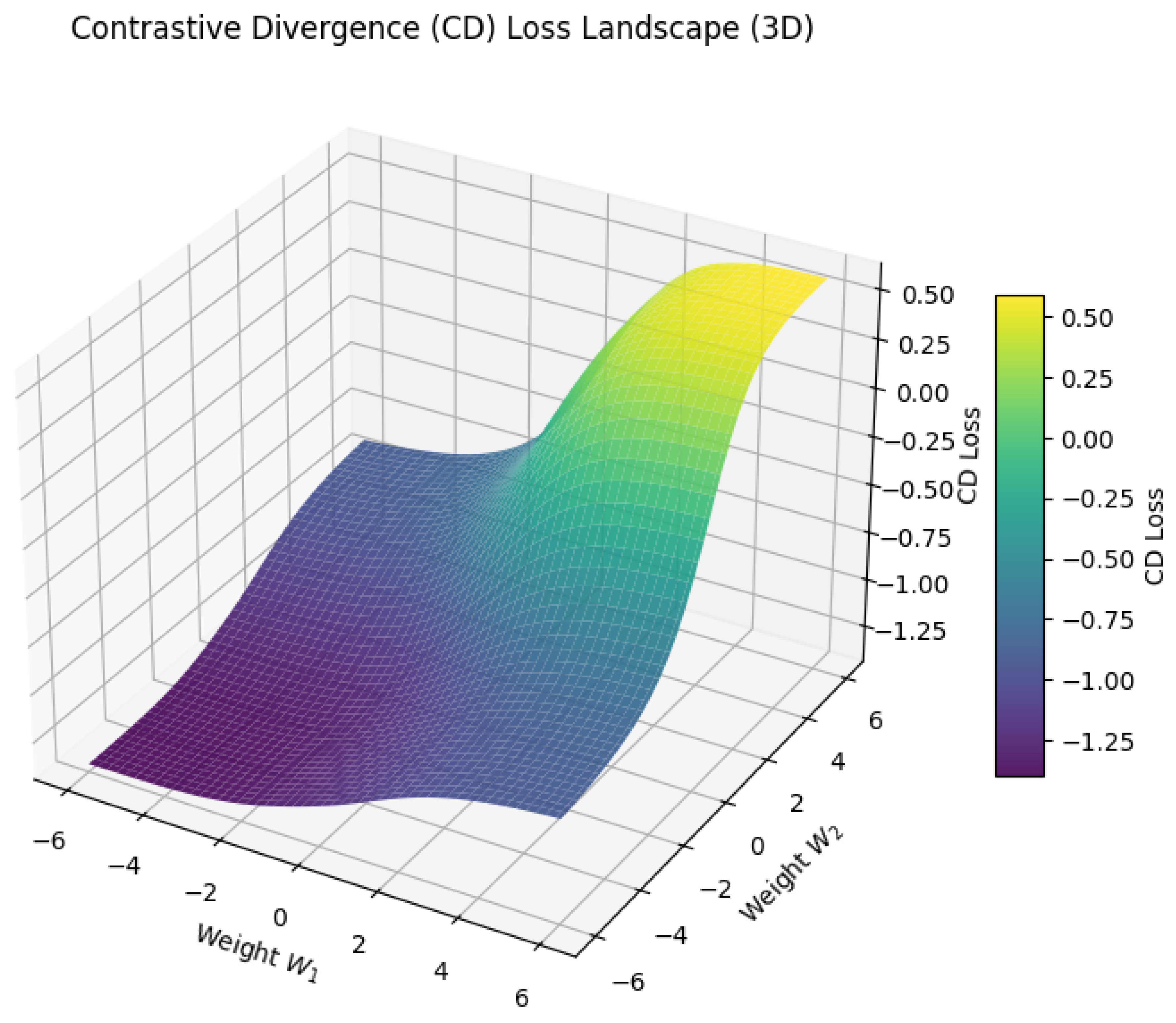
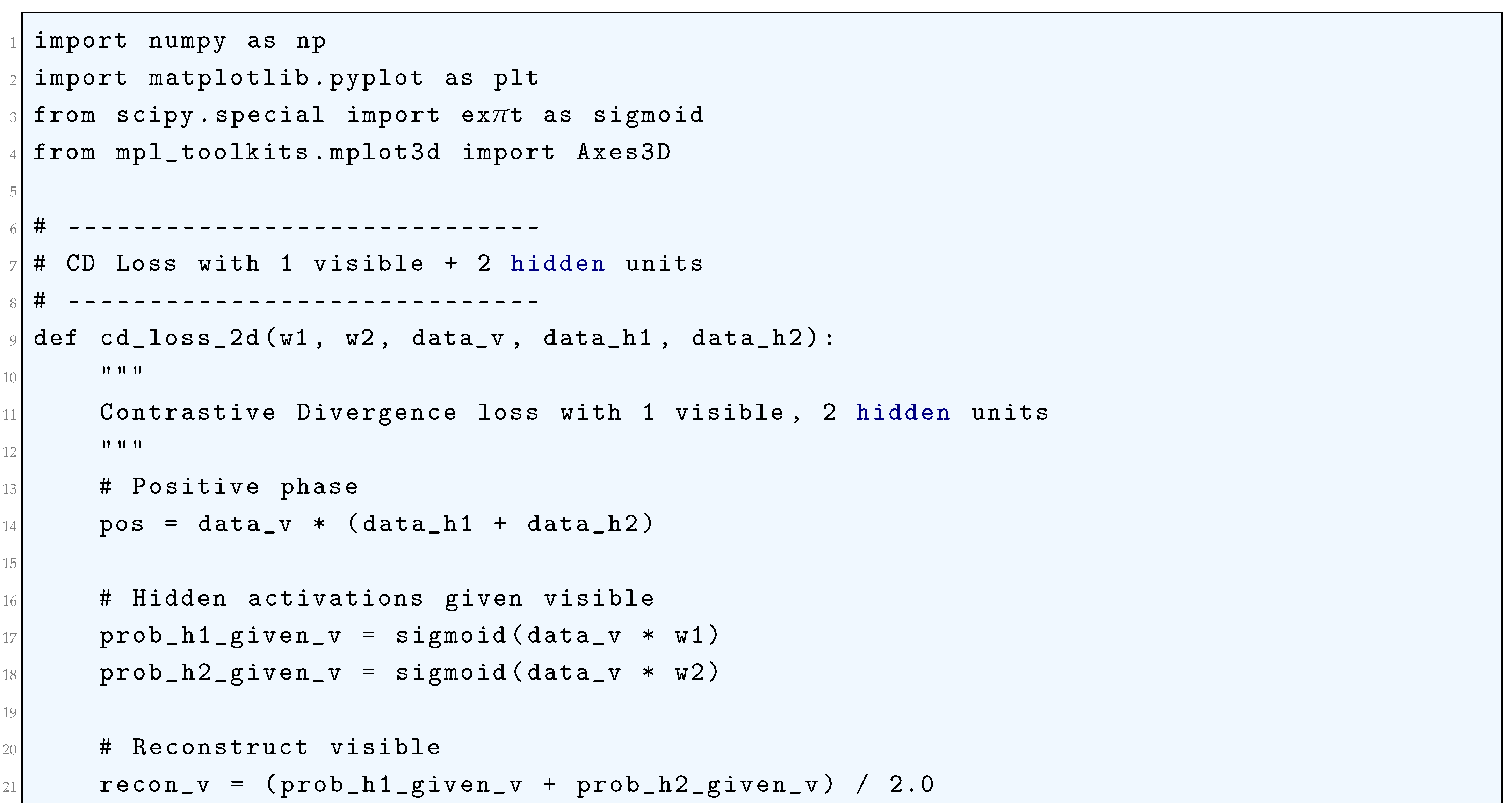
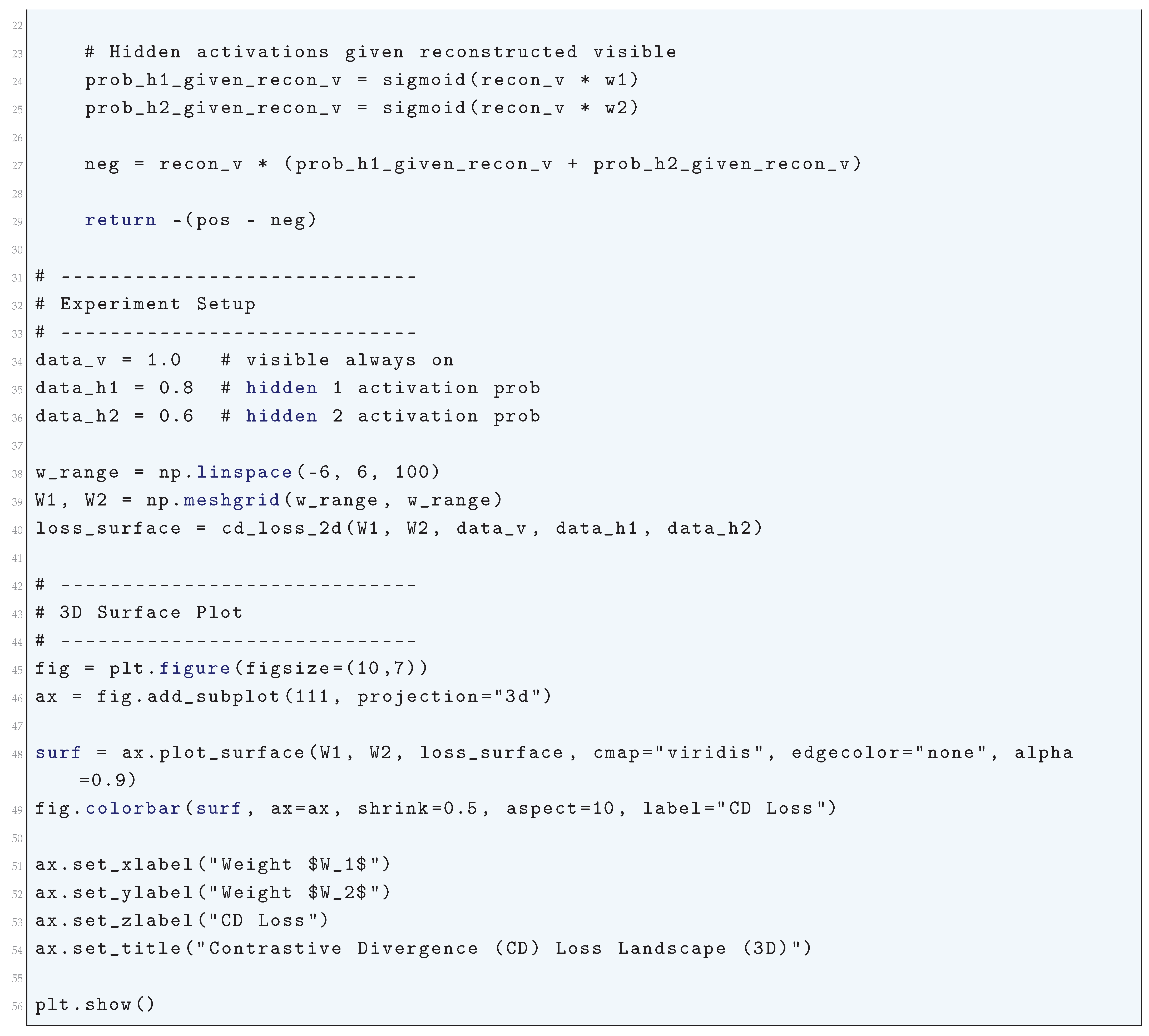
10.5.3.73 Python Code to Generate Figure 140 Illustrating Persistent Contrastive Divergence (PCD) Loss Landscape
The Python code below produces the Figure 140 illustrating Persistent Contrastive Divergence (PCD) Loss Landscape.
Figure 140.
Persistent Contrastive Divergence (PCD) Loss Landscape
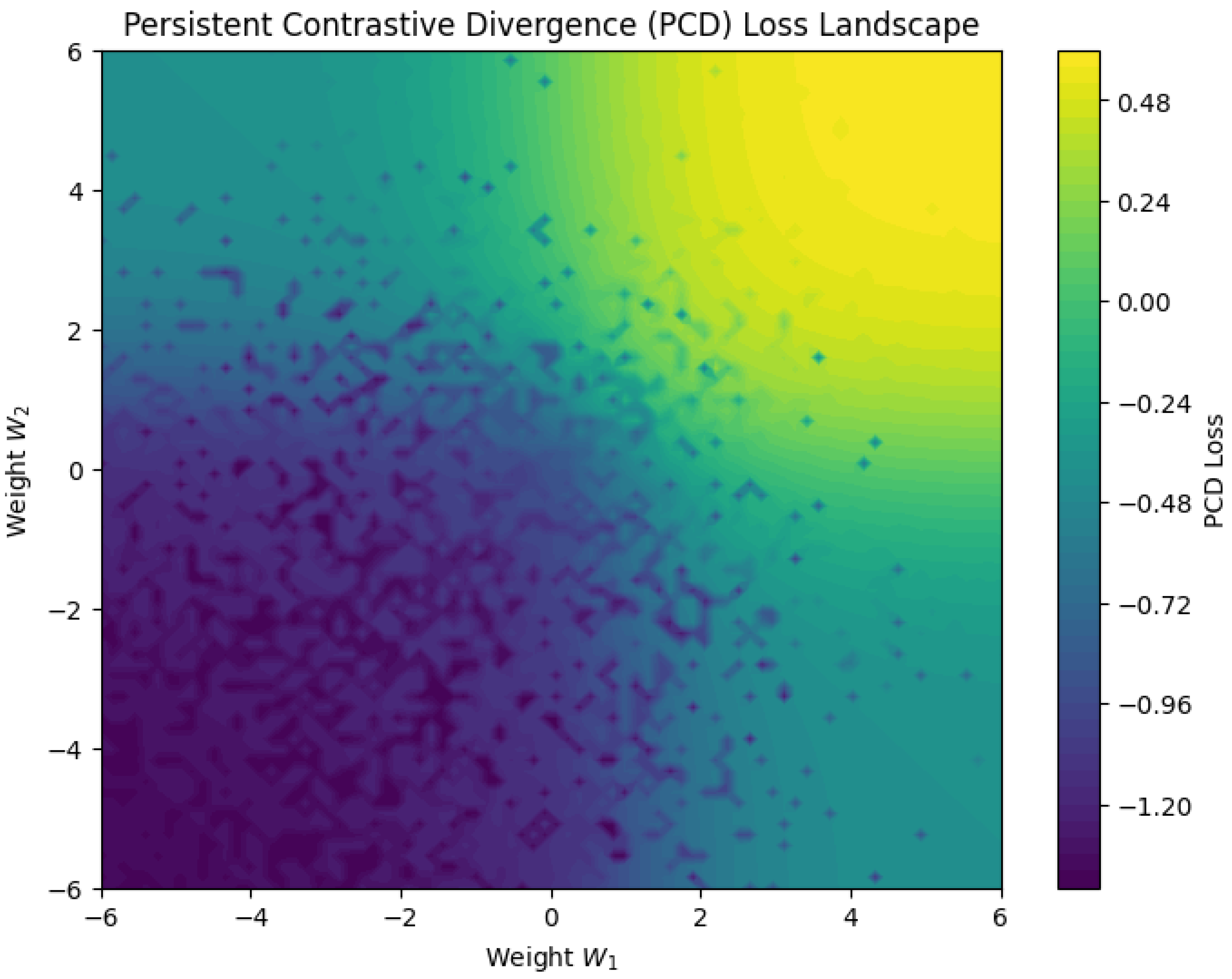
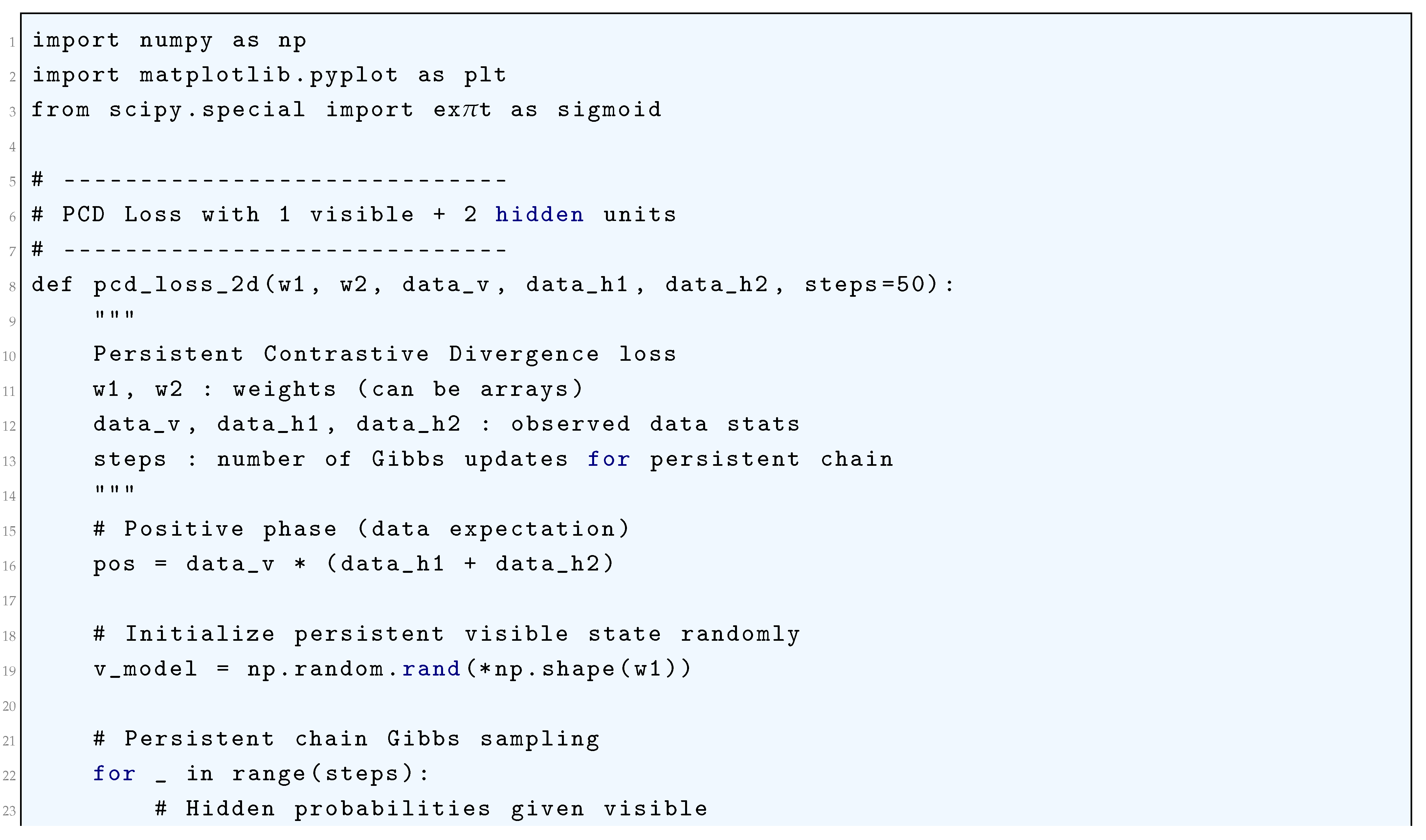
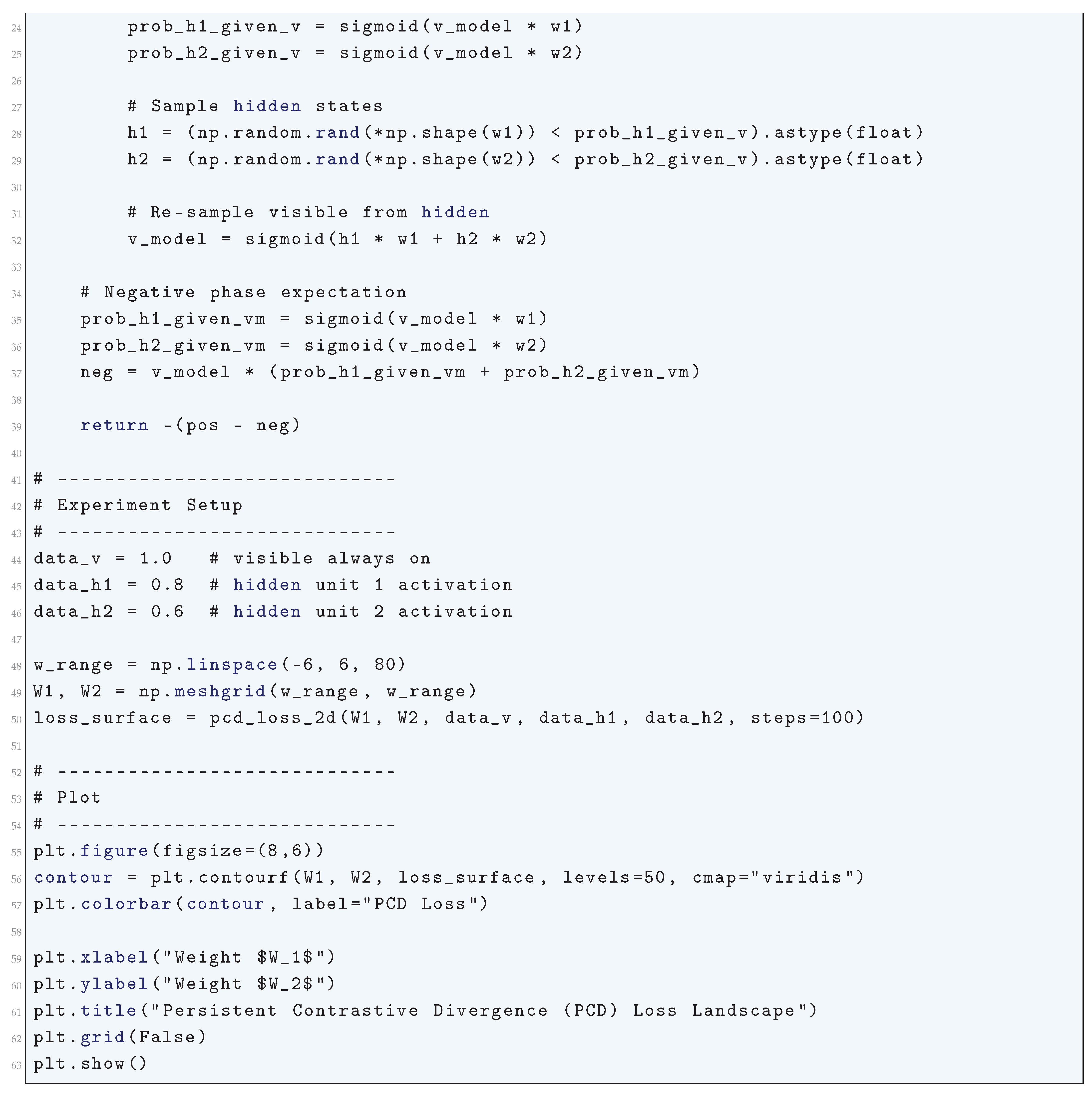
10.5.3.74 Python Code to Generate Figure 141 Illustrating Persistent Contrastive Divergence (PCD) Loss Landscape (3D)
The Python code below produces the Figure 141 illustrating Persistent Contrastive Divergence (PCD) Loss Landscape (3D).
Figure 141.
Persistent Contrastive Divergence (PCD) Loss Landscape (3D)
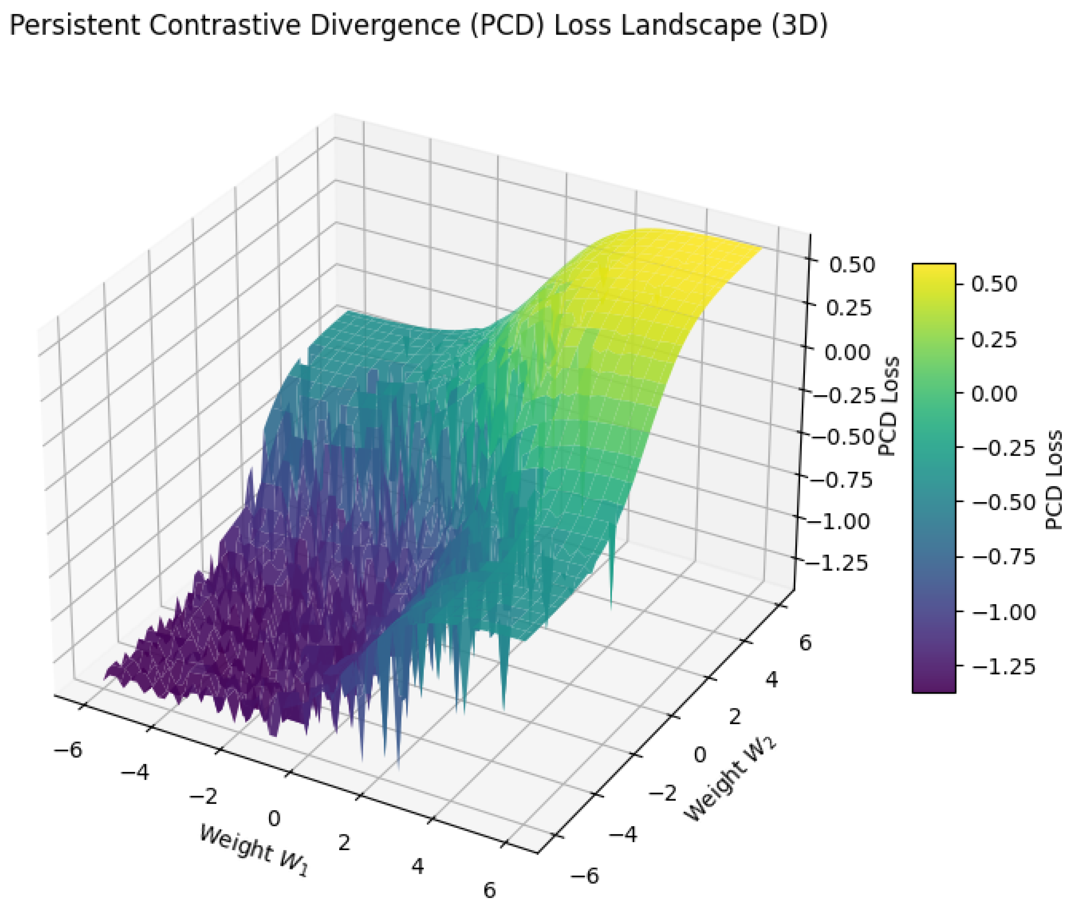
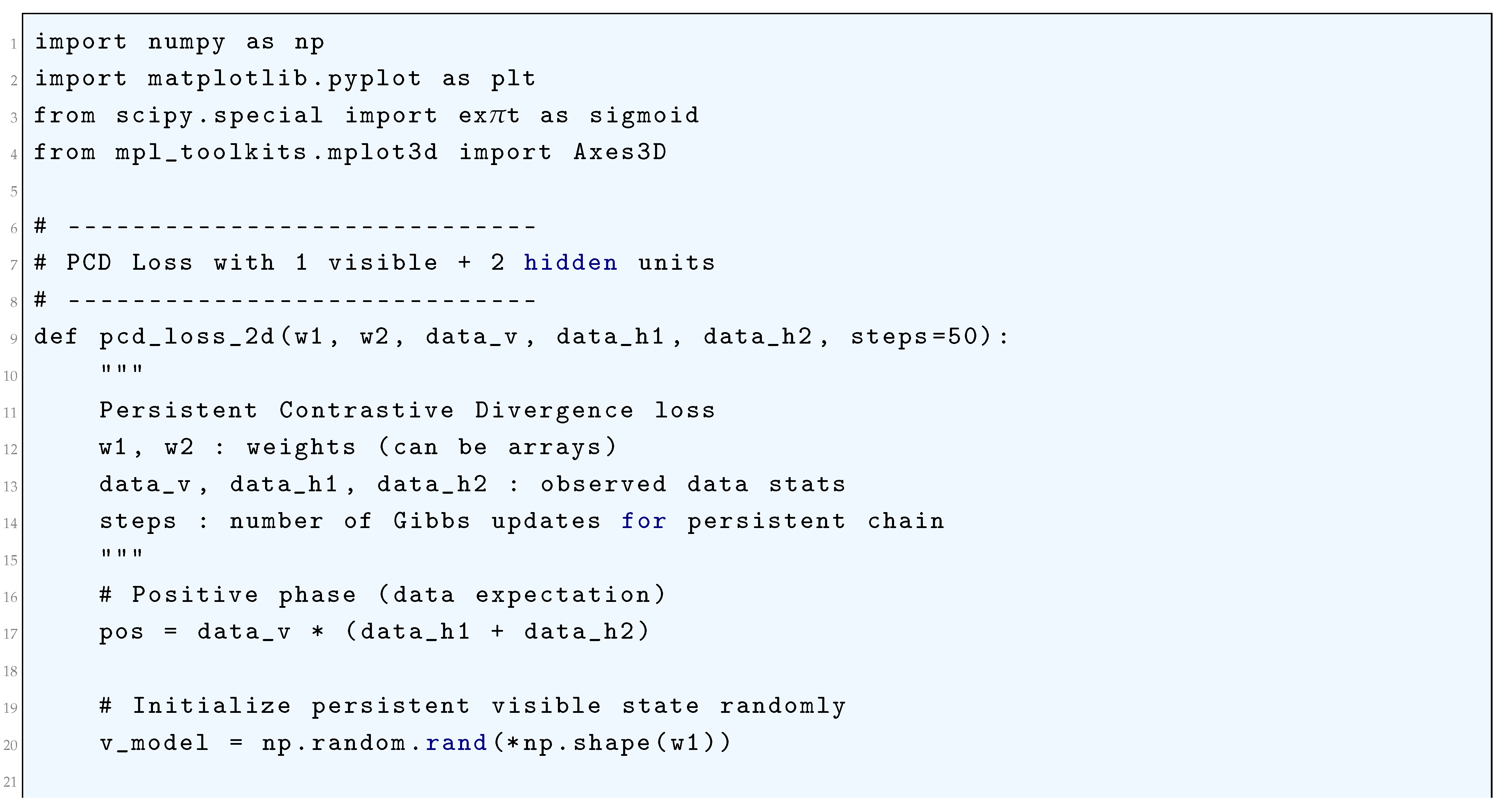
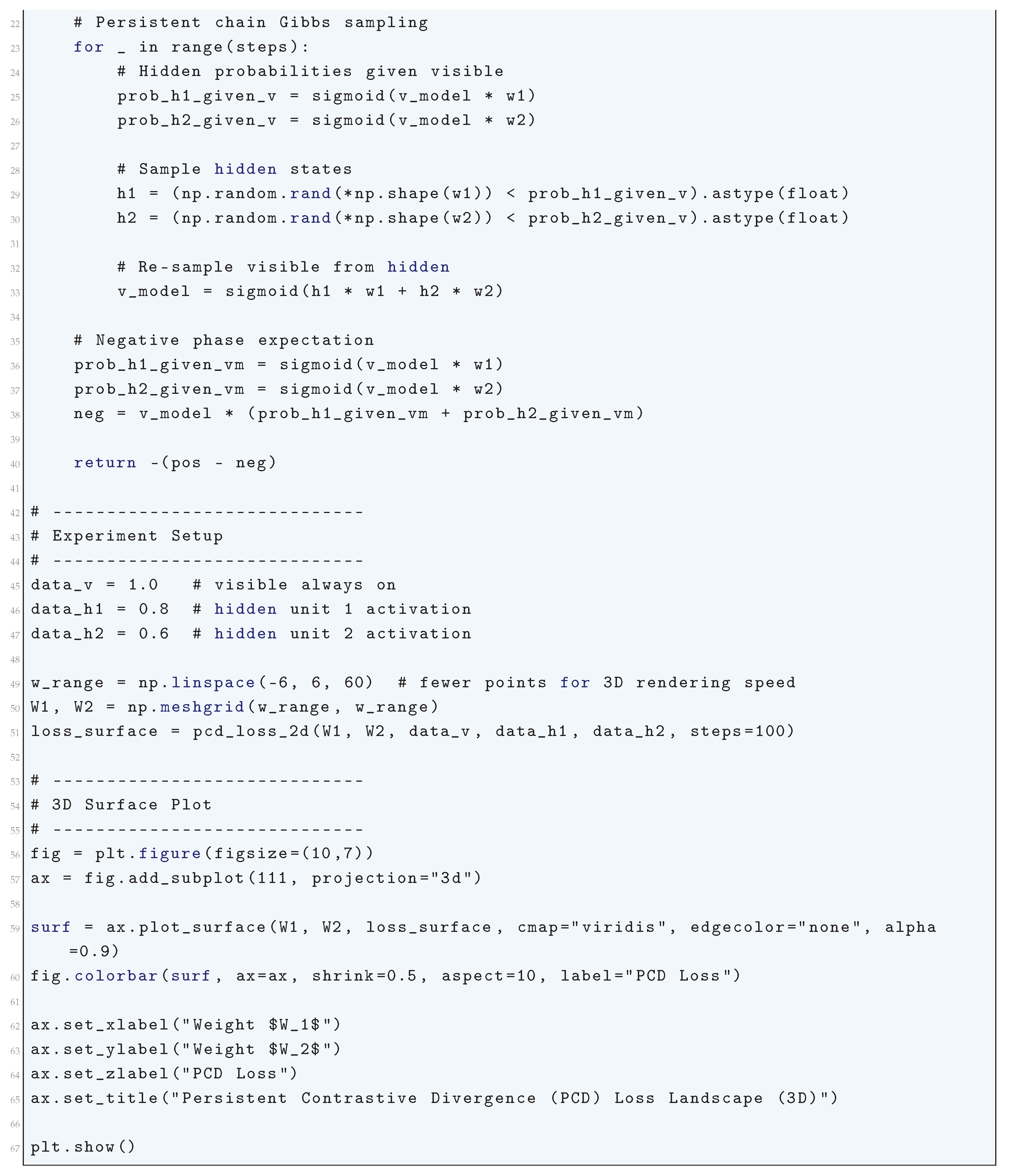
10.5.3.75 Python Code to Generate Figure 142 Illustrating Hausdorff Distance Loss Visualization
The Python code below produces the Figure 142 illustrating Hausdorff Distance Loss Visualization.
Figure 142.
Hausdorff Distance Loss Visualization
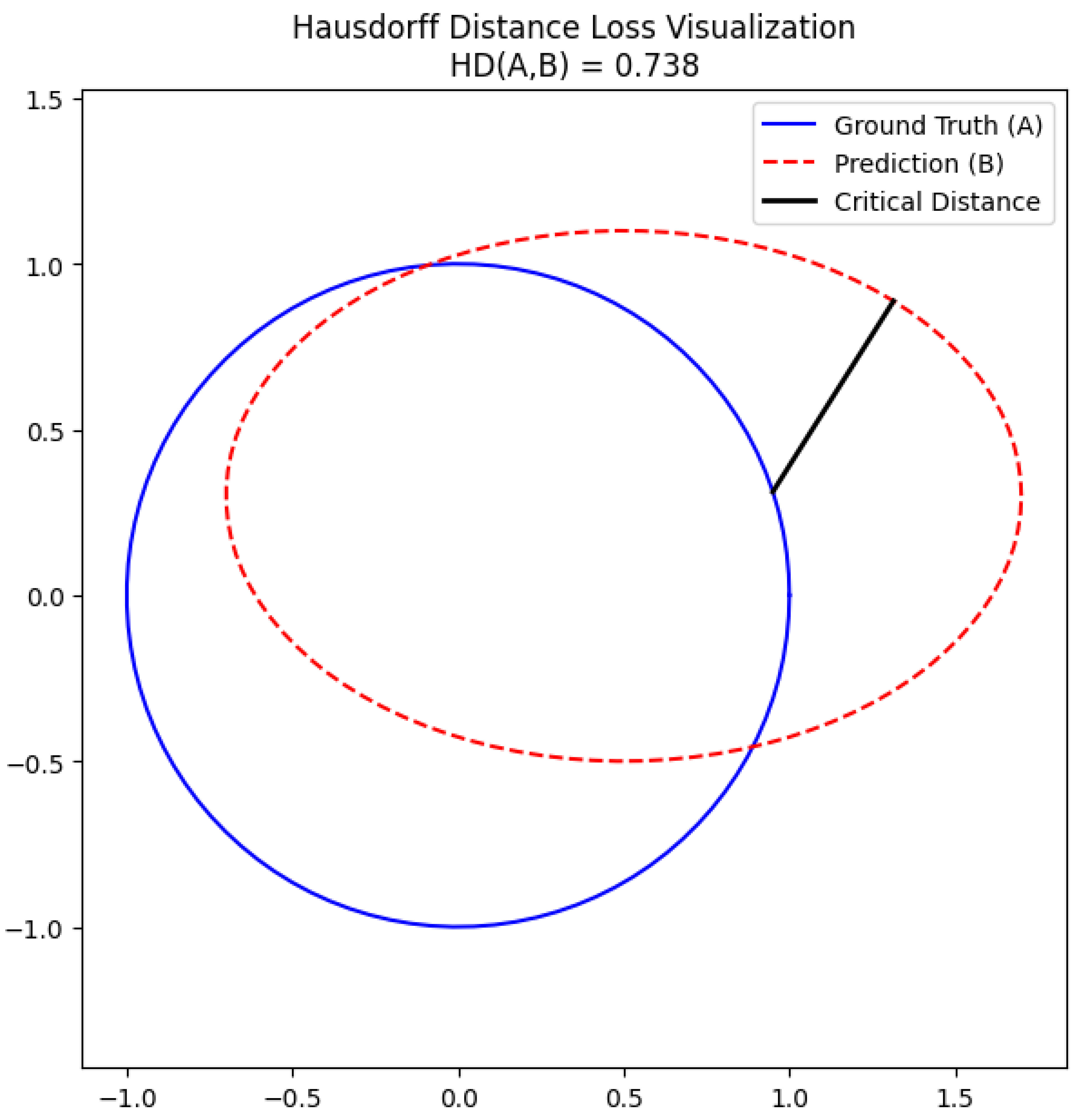
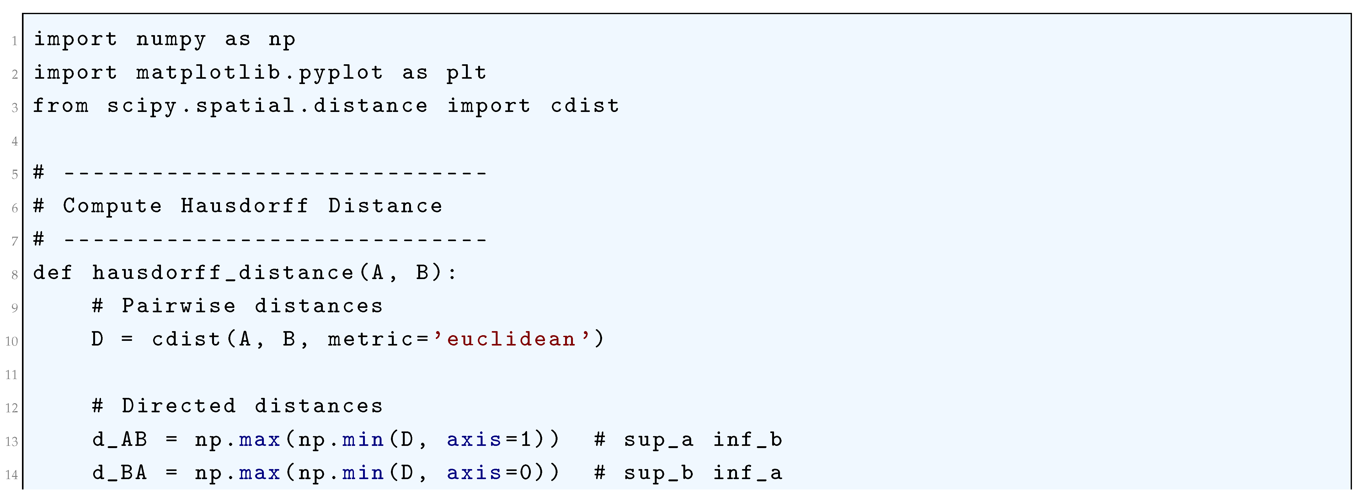
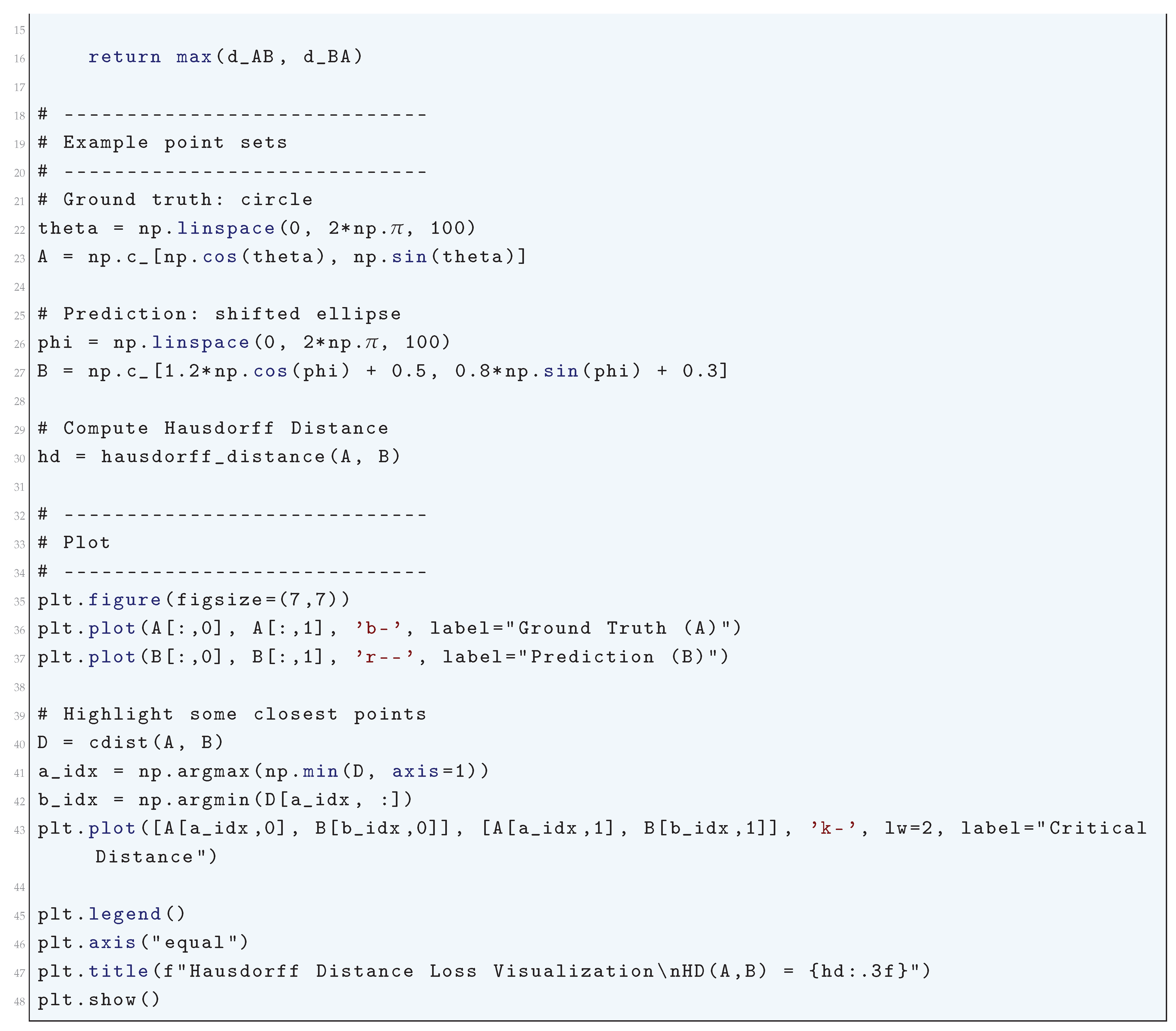
10.5.3.76 Python Code to Generate Figure 143 Illustrating Hausdorff Distance Heatmap
The Python code below produces the Figure 143 illustrating Hausdorff Distance Heatmap.
Figure 143.
Hausdorff Distance Heatmap
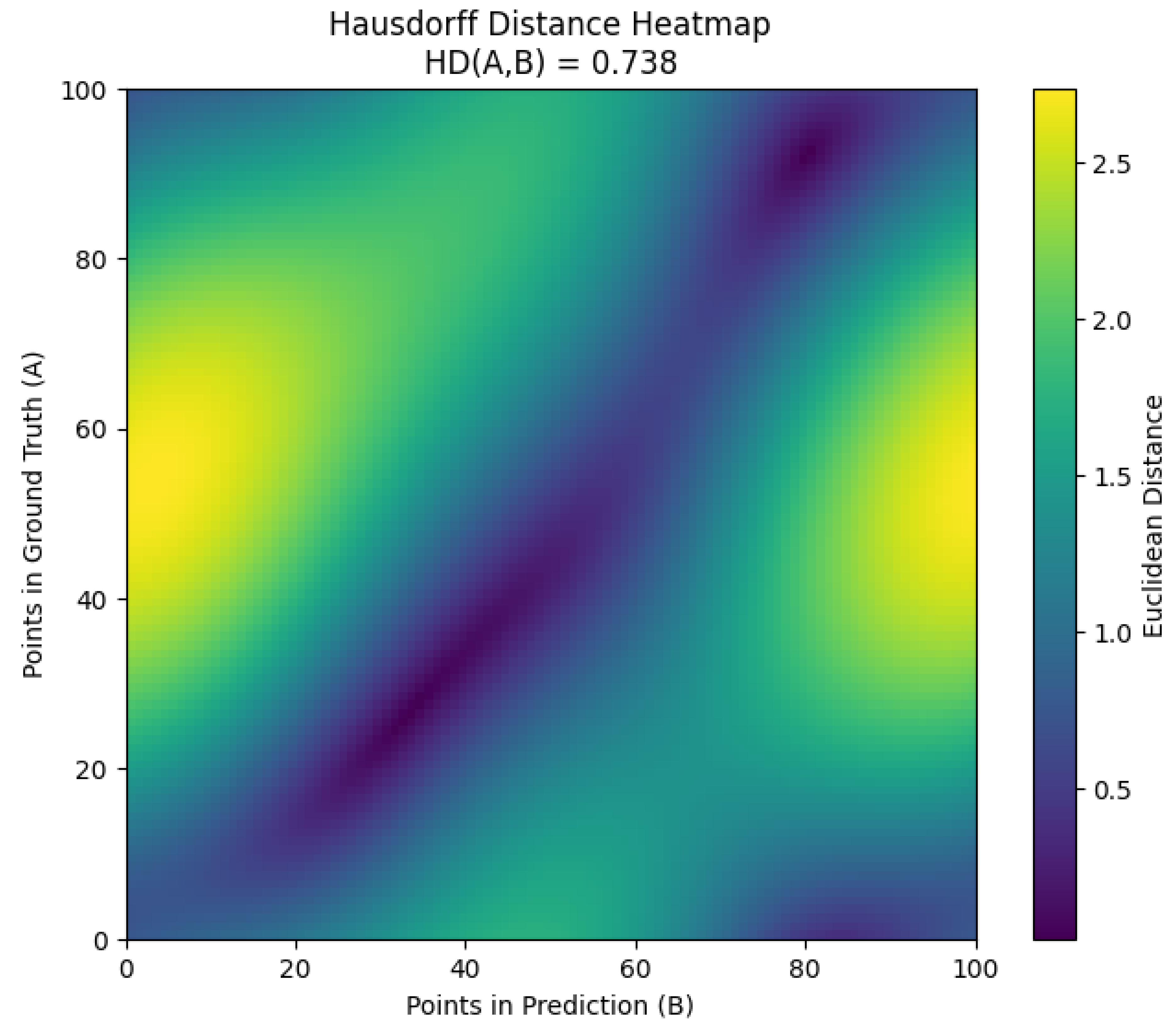
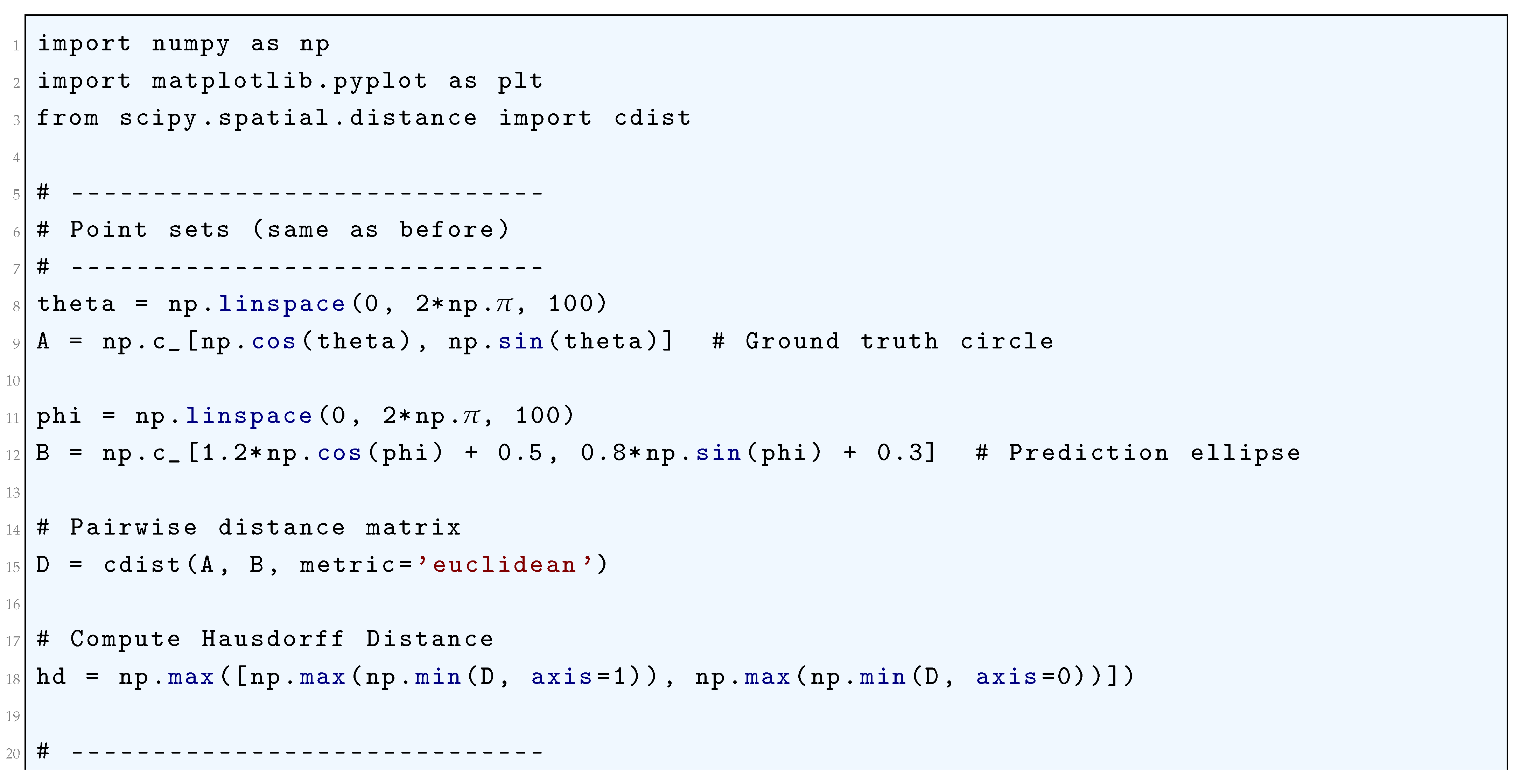
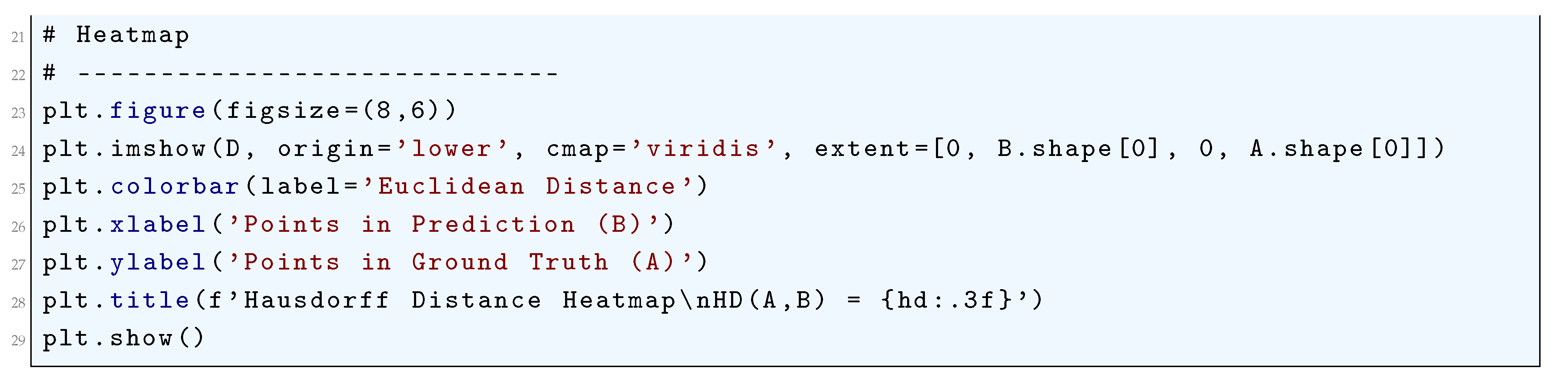
11. Few-Shot Learning
Few-shot learning (FSL) refers to the problem of training a model to generalize to new tasks using only a limited number of labeled examples. Mathematically, given a dataset consisting of N labeled instances, a conventional supervised learning model aims to learn a mapping by minimizing an empirical risk functional of the form
where is an appropriate loss function such as the cross-entropy loss
where denotes the model parameters. However, in a few-shot setting, the number of labeled examples per class is very small, typically denoted as K, where , making it challenging to generalize in a conventional learning paradigm. Few-shot learning is often formalized using meta-learning approaches where the goal is to optimize a learning algorithm itself such that it can quickly adapt to new tasks using very few labeled samples. A common meta-learning formulation involves the optimization of a meta-objective defined over a distribution of tasks . Given a distribution , a meta-learner optimizes parameters such that the expected loss over tasks is minimized:
where each task consists of a small training set (the support set) and a validation set (the query set). The loss function for a given task is typically written as:
where denotes the model adapted using the small support set . A well-known approach to FSL is Model-Agnostic Meta-Learning (MAML), where the optimization is performed by updating such that it rapidly adapts to new tasks via a few gradient updates. Specifically, MAML defines a bi-level optimization problem where an inner loop computes task-specific parameters via gradient descent:
where is the step size. The outer loop then updates based on the loss incurred on the query set:
where is another learning rate. The goal of MAML is to find an initialization such that a small number of gradient steps suffices for good generalization. Another prominent FSL approach is metric-based learning, where models learn an embedding function such that a similarity function enables effective classification in a low-data regime. A widely used method is prototypical networks, which represent each class in the support set with a prototype:
where is the subset of the support set corresponding to class k. Classification is then performed using a softmax function over distances:
where is typically the squared Euclidean distance. The training objective is the negative log-likelihood:
Bayesian methods in FSL adopt a probabilistic framework where uncertainty in model parameters is explicitly modeled using a prior . Given a support set , a Bayesian model infers a posterior over parameters:
A predictive distribution over a new query point is obtained by marginalizing over :
Ultimately, the success of FSL hinges on leveraging shared structure across tasks, designing effective adaptation mechanisms, and optimizing inductive biases to mitigate data scarcity.
11.1. Meta-Learning Formulation in Few Shot Learning
Meta-learning, particularly in the context of Few-Shot Learning (FSL), aims to train a model such that it can generalize effectively to novel tasks with very few training examples. This is accomplished by optimizing the learning process itself, enabling the model to rapidly adapt to new tasks. Given a distribution over tasks , where each task is characterized by a small support set and a corresponding query set , the objective of meta-learning is to train a model with parameters such that it minimizes the expected loss over new tasks drawn from .
where represents the loss function associated with the task , typically computed over the query set after adapting the model using the support set. One of the most widely used meta-learning approaches is Model-Agnostic Meta-Learning (MAML), which optimizes for an initial parameter set that can be quickly adapted to a new task using only a few gradient steps. The inner-loop adaptation updates the model parameters as:
where is the inner-loop learning rate. The meta-objective then minimizes the loss computed on the query set with respect to the updated parameters:
which requires computing the meta-gradient:
leading to the final meta-update:
where is the meta-learning rate. Another formulation follows metric-based meta-learning, where the model learns an embedding function that maps input samples to a feature space where classification can be performed using a simple distance metric. In Prototypical Networks, the class prototype for each class c in the support set is computed as:
where is the set of examples belonging to class c. The probability of assigning a query sample to class c is then given by:
where is a distance metric, often chosen as the squared Euclidean distance. Contrastive learning-based meta-learning methods instead optimize a loss function based on relative similarities. A common choice is the contrastive loss:
where m is a margin parameter and is an indicator function. Bayesian meta-learning approaches introduce a probabilistic treatment where the model parameters are sampled from a learned posterior distribution , updated via variational inference:
where denotes the Kullback-Leibler divergence. The expected posterior predictive distribution for a new task is then computed as:
which can be approximated using Monte Carlo sampling. Gradient-based meta-learning methods can also be formulated using recurrent neural networks, where the meta-learner is a recurrent model that updates a task-specific hidden state over a sequence of examples. Given a sequence of support set updates, the parameterized recurrence is given by:
and the model parameters for a given task are inferred as:
where and are recurrent function approximators parameterized by . These meta-learning paradigms share a common objective: to minimize the expected generalization error of a model trained over a distribution of tasks, enabling rapid adaptation to new scenarios with minimal labeled data. The fundamental mechanism across formulations involves optimizing a bi-level objective where the outer loop adjusts meta-parameters and the inner loop performs task-specific adaptation. The optimization problem governing this framework can be expressed in a general form as:
which encapsulates the core philosophy of meta-learning: learning to learn.
11.2. Bayesian Methods in Few Shot Learning
Bayesian methods in Few-Shot Learning (FSL) provide a principled probabilistic framework for reasoning about uncertainty in the context of limited data. The core objective of FSL is to train a model on a set of "base" classes with abundant data such that it can rapidly generalize to a set of novel classes, for which only a few labeled examples (the support set S) are provided. The Bayesian approach treats the model parameters, or more commonly a task-specific context, as latent random variables, enabling the quantification of epistemic uncertainty arising from the scarcity of data. This is fundamentally expressed through Bayes’ theorem. Let D represent the support set for a novel task, and let represent the model parameters or task-specific adaptation parameters. The posterior distribution over these parameters is given by
where is the prior distribution encapsulating knowledge acquired from the base classes, is the likelihood of the support data, and
is the model evidence. The intractability of this evidence integral necessitates approximate inference techniques.
A prominent Bayesian formulation for FSL involves placing a prior over the parameters of the classifier for novel classes, while the feature embedding network is considered fixed and learned during meta-training. For a N-way, K-shot task, the support set is
The goal is to infer the parameters of the novel-class classifier. A hierarchical Bayesian model posits
where are hyperparameters learned from the base classes. The prior regularizes the novel class classifier. For a linear classifier where , a common prior is an isotropic Gaussian,
The likelihood for the support set, assuming a softmax classification model, is
where W is the matrix of weight vectors and is the feature embedding function. The posterior is then used for prediction on a query point via
Direct computation of the posterior is analytically intractable due to the non-conjugacy of the softmax likelihood and the Gaussian prior. Therefore, variational inference is extensively employed. In this framework, a parameterized variational distribution is introduced to approximate the true posterior. The goal is to minimize the Kullback-Leibler (KL) divergence between the variational approximation and the true posterior, . This is equivalent to maximizing the Evidence Lower Bound (ELBO),
The parameters of the variational distribution are optimized during this inference step. For example, if
then . The expectation is typically estimated via Monte Carlo sampling,
where . The predictive distribution for a query point becomes
marginalizing over the posterior uncertainty.
An alternative and highly influential Bayesian perspective is embodied by the framework of Bayesian meta-learning, particularly through models like the Neural Process and its variants. Here, the entire context of the support set is used to define a latent variable z that represents the task. The generative model for a task is
The conditional likelihood is implemented by a decoder network. The posterior over the task variable given the support set is
Inference is again performed approximately, often using a variational inference scheme where an encoder network amortizes the inference process by mapping the entire support set to a distribution over z. The ELBO for this model is
where are the decoder parameters. The predictive distribution for a query point is
with .
Gaussian Processes (GPs) offer another rigorously Bayesian non-parametric approach to FSL. A GP defines a prior directly over functions,
where is the mean function and is the covariance kernel function. In the FSL setting, the support set S conditions this prior to yield a posterior process. The key equations for prediction are derived from the joint Gaussian distribution of the support and query points. Let and be the inputs and labels of the support set, and be the query inputs. The joint prior is
where for , and similarly for . For regression, the posterior predictive distribution is Gaussian:
with
and
For classification, a likelihood , such as a Bernoulli-logit, is introduced, and the posterior becomes non-Gaussian, requiring approximation methods like Laplace approximation or expectation propagation.
The Bayesian treatment naturally allows for the integration of uncertainty into the learning process itself, a concept formalized in Bayesian optimization for hyperparameter tuning in FSL. The acquisition function, which guides the search for optimal hyperparameters , leverages a surrogate model for the objective function . Given a prior over functions, typically a GP, and observed data , the posterior is used to compute an acquisition function such as Expected Improvement (EI),
where is the current best hyperparameter configuration. This rigorous probabilistic framework for hyperparameter selection is crucial in FSL where the risk of overfitting to the few shots is high. The unifying theme across all these Bayesian methods is the explicit representation of uncertainty through probability distributions, transforming the few-shot learning problem from a point-estimation task into one of full posterior inference, thereby enhancing robustness and calibration.
11.3. Prototypical Networks in Few Shot Learning
Prototypical networks operate within the framework of few-shot classification by learning a non-linear embedding of input data into a metric space where classification can be performed by computing distances to prototype representations of each class. The foundational assumption is that there exists an embedding function with parameters that maps inputs into a d-dimensional space such that points cluster around a single prototype representation for each class. Given a support set where is an input and is its corresponding class label, the prototype for each class k is computed as the mean vector of the embedded support points belonging to that class. This computation is formally expressed by the equation
where denotes the set of support examples labeled with class k.
For a query point x, the prototypical network produces a distribution over classes based on a softmax over the negative distances from the embedded query point to the class prototypes. The distance metric is typically the squared Euclidean distance in the embedding space, defined as
The probability that the query point x belongs to class k is then given by
This formulation aligns with the concept of a Gibbs distribution, where the negative distance acts as an energy function, making the probability proportional to the exponentiated similarity between the query embedding and the class prototype.
The training objective is to maximize the likelihood of the true class for all query points across training episodes, which is equivalent to minimizing the negative log-probability. For a single episode with support set S and a query set Q, the loss function is defined as
where is the true class label of the query point . Substituting the probability expression, the loss becomes
This can be simplified to
which is effectively a cross-entropy loss computed in the metric space.
The learning process occurs through episodic training. Each episode is constructed by randomly selecting a subset of classes , then for each class , selecting a support set and a query set . The complete support set for the episode is and the query set is . The prototypes for all are computed from S, and the parameters of the embedding network are updated by performing a gradient descent step on the loss computed on Q. The update rule is
where is the learning rate. The gradients flow through both the query point embeddings and the prototype computations, as the prototypes are functions of via the support examples. The gradient of the loss with respect to a prototype vector is
where is the indicator function. The gradient with respect to the embedding of a support point is
and the gradient with respect to the embedding of a query point is
The scientific rigor of this approach is rooted in its interpretation as a form of mixture density estimation on the embedded space. If each class-conditional distribution in the embedding space is a spherical Gaussian with a fixed, shared covariance matrix , then the probability density for a point under class k is
Assuming equal prior probabilities for all classes, the posterior probability for class k given z is
By setting , this posterior simplifies exactly to the softmax over negative squared Euclidean distances used in the prototypical network,
This probabilistic foundation provides a rigorous justification for the model’s architecture and loss function, framing it as an approximate inference procedure under a specific generative model of the data in the embedding space. The model’s efficacy is thus contingent upon the embedding network’s ability to transform the input data such that its distribution in the latent space conforms to this isotropic Gaussian assumption per class.
11.4. Model-Agnostic Meta-Learning (MAML) in Few Shot Learning
Model-Agnostic Meta-Learning (MAML) is a fundamental optimization-based approach in few-shot learning, designed to enable models to quickly adapt to new tasks with minimal data. The core idea is to learn an initialization of model parameters that facilitates rapid adaptation through gradient-based updates. Given a distribution over tasks, denoted as , MAML optimizes for a set of parameters such that for a new task , the adapted parameters after a small number of gradient steps yield high performance on the task.
For a given task , we assume a dataset composed of a support set and a query set . Let the model be parameterized by and let the task-specific loss function be . The adaptation to task involves performing one or more gradient descent steps with respect to evaluated on . The standard first-order adaptation rule for a single gradient step is given by:
where is the learning rate for task-specific updates. The meta-objective is to find an initialization such that after task-specific adaptation, the model performs well on the query set . The meta-loss is computed over the query set:
which leads to the outer-level optimization of :
where is the meta-learning rate. Expanding the gradient term using the chain rule,
with
where I is the identity matrix and is the Hessian of the loss function with respect to . The optimization process involves computing second-order derivatives, which can be computationally expensive. A first-order approximation, called First-Order MAML (FOMAML), simplifies this update by ignoring the Hessian term:
where is still obtained using the standard gradient descent update. This approximation reduces computational overhead while still achieving strong meta-learning performance. The effectiveness of MAML depends on its ability to learn an initialization that allows rapid adaptation across a diverse set of tasks. Formally, we define the expected meta-loss over the task distribution:
which represents the expectation over the loss incurred after a single adaptation step. The meta-optimization aims to minimize this expected loss, ensuring that provides an effective starting point for task-specific fine-tuning. For multiple gradient adaptation steps, the parameter update for a given task follows an iterative process:
for , where K denotes the number of inner-loop gradient updates. The final adapted parameters are then used to compute the meta-loss:
which determines the outer-loop optimization of . The full meta-gradient computation involves backpropagating through K gradient updates, leading to higher-order derivative terms:
where each term captures the second-order effects of iterative gradient updates.
11.5. Metric-Based Learning in Few Shot Learning
Metric-based learning in the context of few-shot learning is a paradigm that relies on learning a similarity metric to compare query examples against a set of labeled support examples. Given a support set , where each is an input instance and is its corresponding label, and a query instance , the goal is to predict based on a learned metric function parameterized by . The fundamental principle is that instances belonging to the same class should be mapped closer together in an embedding space, while instances from different classes should be mapped further apart. Mathematically, this can be formulated as minimizing the intra-class variance while maximizing the inter-class variance, which can be written as
where is a weighting factor that controls the relative importance of inter-class separation. The metric function is often implemented using a neural network that maps instances into an embedding space via an encoder , such that
One of the key approaches in metric-based few-shot learning is prototypical networks, where each class in the support set is represented by a prototype , computed as the mean of embedded support examples belonging to class k:
The classification of a query example is then performed by computing its similarity to each prototype, typically using the squared Euclidean distance,
Another prominent approach is relation networks, which replace the explicit distance metric with a learned similarity function , parameterized by . The probability of assigning query to class k is given by
Siamese networks approach metric learning through pairwise comparisons, where a shared encoder maps pairs of examples into an embedding space, and the similarity is computed as
where W is a learned weight vector and is the sigmoid activation function. The model is trained to minimize the binary cross-entropy loss,
Triplet networks extend this by considering an anchor example , a positive example (same class), and a negative example (different class), enforcing the constraint
where m is a margin hyperparameter. The loss function is given by
By optimizing these loss functions, metric-based few-shot learning methods enable models to generalize well to novel classes, as the learned metric encodes class-invariant representations of instances. The embedding space acts as a structured manifold where geometric distances capture semantic similarities, allowing rapid adaptation to unseen tasks with minimal labeled data.
11.6. Bayesian Methods in Few Shot Learning
Bayesian methods in Few-Shot Learning (FSL) provide a probabilistic framework to model uncertainty in learning from a small number of examples. Given a dataset with a limited number of training examples N, Bayesian approaches aim to infer a distribution over the model parameters , rather than a single deterministic estimate, allowing the model to generalize effectively despite limited data. The core idea is to use Bayes’ theorem to compute the posterior distribution over :
where is the likelihood of the data given parameters , is the prior over the parameters, and is the marginal likelihood or evidence. The posterior distribution encapsulates the uncertainty in parameter estimation, making it particularly useful for FSL where the data is scarce.
The Bayesian framework enables meta-learning by assuming that tasks in FSL are drawn from an unknown distribution over tasks . Given a set of tasks , each with a small support set and query set , the goal is to learn a distribution over task-specific parameters conditioned on the support set:
A hierarchical Bayesian model treats the task-specific parameters as drawn from a global distribution with hyperparameters :
where defines a prior distribution over . This enables the model to generalize across tasks by updating the prior using multiple tasks:
Given a new task with support set , the predictive distribution over labels for query inputs is obtained by marginalizing over :
Since exact inference of is often intractable, variational inference is commonly used. We approximate with a variational distribution , parameterized by , minimizing the Kullback-Leibler (KL) divergence:
This leads to an optimization problem where is updated via gradient descent to minimize , ensuring the learned distribution approximates the true posterior. Another approach is Bayesian nonparametrics, where the distribution over functions is modeled using a Gaussian Process (GP), providing a principled way to quantify uncertainty. Given a prior GP:
where is the mean function and is the covariance function, the posterior over functions given training data is:
where and are the posterior mean and covariance functions derived using Bayes’ rule. The predictive distribution for a new input follows:
which yields a closed-form Gaussian predictive distribution due to the properties of GPs. Another key Bayesian technique is Bayesian Neural Networks (BNNs), where instead of learning a single weight matrix W, a distribution over weights is maintained:
Inference in BNNs requires approximations like Monte Carlo Dropout, where approximate Bayesian inference is performed by applying dropout at both training and test time, yielding an empirical posterior:
where are sampled from the variational posterior . This captures uncertainty in predictions, crucial for robust few-shot learning. Bayesian optimization further refines FSL by selecting informative examples to maximize learning efficiency. Given an acquisition function based on the posterior predictive distribution:
a new query point is selected to minimize uncertainty and maximize information gain, enhancing generalization from few samples. Thus, Bayesian methods in FSL provide a mathematically rigorous probabilistic framework to model uncertainty, transfer knowledge across tasks, and make robust predictions even with limited training data.
12. Metric Learning
Metric learning is a fundamental concept in machine learning and mathematical optimization, concerned with learning a distance function or similarity measure that captures the underlying structure of data. Given a set of training samples , where each , the objective is to learn a metric function that quantifies the dissimilarity between any two points. A standard choice for is the Mahalanobis distance, which generalizes the Euclidean distance and is defined as
where is a positive semi-definite matrix, i.e., , ensuring that the distance satisfies the properties of a metric. Learning the matrix is the core challenge in metric learning. When , the metric reduces to the standard Euclidean distance:
However, metric learning seeks to optimize such that semantically similar data points have smaller distances than dissimilar points. This is typically formulated as an optimization problem where we enforce constraints on distances between pairs of points. Given a set of pairs (similar pairs) and (dissimilar pairs), the goal is to satisfy
for some thresholds u and l. One widely used approach to metric learning is Large Margin Nearest Neighbors (LMNN), which seeks to optimize by minimizing a hinge loss on triplets of points , where is closer to than , i.e.,
where the triplet loss ensures that the distance between similar points is smaller than the distance between dissimilar ones by a margin of at least 1. An alternative approach is the information-theoretic metric learning (ITML) framework, which minimizes the Kullback-Leibler divergence between two Gaussian distributions defined by different Mahalanobis distances:
Deep metric learning extends these concepts by parameterizing the metric function using a neural network with learnable parameters , leading to a learned embedding space where distances are computed as
Instead of learning a linear transformation as in Mahalanobis-based methods, deep metric learning implicitly learns a nonlinear mapping such that the Euclidean distance in the transformed space aligns with semantic similarity. The contrastive loss is commonly used in this context:
Alternatively, the triplet loss is defined as
A more recent approach, the normalized temperature-scaled cross-entropy loss (NT-Xent), utilizes a softmax formulation:
where is the cosine similarity,
By optimizing the metric under these constraints, metric learning produces feature representations that are well-structured for downstream tasks such as retrieval, verification, and clustering.
12.1. Large Margin Nearest Neighbors (LMNN) Approach to Metric Learning
The Large Margin Nearest Neighbors (LMNN) approach to metric learning is a method that aims to learn a Mahalanobis distance metric that optimizes nearest neighbor classification by ensuring that points belonging to the same class remain close while different-class points are separated by a large margin. Given a dataset , where represents a feature vector and denotes its class label, LMNN learns a transformation matrix such that the squared distance between any two points is given by
where is a positive semi-definite (PSD) matrix. The optimization problem is designed to minimize classification error by enforcing that each sample remains close to its target neighbors, denoted by , while keeping different-class points at a distance. The objective function consists of two competing terms: a pull term that encourages proximity among target neighbors and a push term that enforces a large margin separation from impostors (samples of different classes that intrude upon the local neighborhood). The pull term is formulated as
This term ensures that the squared distances between each point and its target neighbors remain small. The push term, on the other hand, ensures that impostors—points of a different class than but closer than its farthest target neighbor—are pushed away by at least a margin 1, formulated using hinge loss as
subject to the constraints
The total LMNN objective function combines these terms as
where C is a regularization parameter controlling the tradeoff between the pull and push terms. The constraint ensures that the learned metric remains a valid Mahalanobis distance. The optimization is typically solved using semidefinite programming (SDP) or projected gradient descent methods while enforcing the PSD constraint on . To interpret the impact of the learned metric, consider an eigenvalue decomposition of , given by
where is an orthonormal matrix and is a diagonal matrix of eigenvalues. The transformation effectively maps the original data space into a new space where distances are reshaped to optimize nearest-neighbor classification performance. The LMNN framework ensures that different classes are well-separated while preserving local neighborhood structures, leading to improved generalization in classification tasks.
12.2. Information-Theoretic Metric Learning (ITML) Framework Approach to Metric Learning
The Information-Theoretic Metric Learning (ITML) framework is a fundamental approach to metric learning that formulates the problem as an optimization task driven by information theory principles, particularly Kullback-Leibler (KL) divergence minimization. Given a set of data points , the goal of ITML is to learn a Mahalanobis distance metric parameterized by a positive semi-definite (PSD) matrix , so that distances between similar points are minimized while distances between dissimilar points are maintained above a certain threshold. The Mahalanobis distance between two points and under the learned metric is defined as
where is a symmetric positive semi-definite matrix, i.e., , ensuring that defines a proper distance function. The fundamental idea of ITML is to find a metric that minimizes the divergence from a given prior metric , typically the identity matrix , subject to constraints that enforce distances between pairs of points to satisfy specified conditions. To formalize this, ITML minimizes the KL divergence between the distributions parameterized by and . Given that Gaussian distributions parameterized by a Mahalanobis metric have a natural representation in terms of covariance matrices, the KL divergence between two Gaussian distributions with covariance matrices and is
where denotes the trace operator, and is the logarithm of the determinant. The optimization problem in ITML is thus formulated as
subject to pairwise constraints of the form
where and denote sets of similar and dissimilar pairs, respectively, and are predefined thresholds that control the tightness of the constraints. The use of KL divergence as the objective function ensures that the learned metric remains close to the prior while satisfying the constraints. To solve this optimization problem, a log-barrier method is commonly employed, leading to an iterative update for of the form
where is an adaptive step size chosen to satisfy the constraints. This iterative procedure ensures that remains positive semi-definite at every step. The learned metric is influenced by the data-driven constraints while maintaining a balance between adaptation and preservation of the prior structure. The ITML framework exhibits strong theoretical properties, particularly in terms of generalization and convexity. Since the optimization problem is convex in , the solution is globally optimal, ensuring robustness. Moreover, the constraint formulation allows for a natural interpretation: if the prior , then the learned metric is a transformation of Euclidean space that deforms distances according to the prescribed similarity relationships. In practice, ITML is highly effective due to its ability to incorporate prior knowledge and adapt flexibly to data distributions. The reliance on KL divergence ensures stability in learning, preventing excessive deviation from the prior. By iteratively refining the metric with convex optimization, ITML efficiently learns a Mahalanobis metric that best captures the underlying relationships within the data.
12.3. Deep Metric Learning
Deep Metric Learning (DML) is a fundamental approach in machine learning that aims to learn an embedding function that maps input data points from a high-dimensional space to a lower-dimensional space , such that semantically similar points are brought closer together while dissimilar points are pushed farther apart. Formally, given a dataset with labels , the goal is to optimize the parameters of the embedding function such that for any triplet of points where (anchor) and (positive) belong to the same class (), while (negative) belongs to a different class (), the Euclidean distance in the embedding space satisfies
where is a margin that enforces a minimum separation between positive and negative pairs. To achieve this objective, DML often employs contrastive loss, which minimizes the Euclidean distance between positive pairs while maximizing it for negative pairs. Given a pair , the contrastive loss function is
where if and belong to the same class, otherwise, is the Euclidean distance, and m is a margin parameter. Another widely used loss function in DML is the triplet loss, given by
This loss function ensures that the anchor-positive distance is always smaller than the anchor-negative distance by at least , thereby enforcing clustering of similar instances while separating dissimilar ones. In deep learning-based metric learning, the embedding function is typically parameterized by a deep neural network such as a convolutional neural network (CNN) for image data or a recurrent neural network (RNN) for sequential data. Let x be an input sample and let the network be denoted as . The network is optimized by minimizing the empirical risk
where represents the data distribution. To further refine the embeddings, methods such as hard negative mining are employed, where the negative samples are chosen such that
This strategy ensures that the network focuses on difficult examples that are closer to the anchor, making learning more effective. To generalize beyond triplet-based losses, one can also consider the N-pair loss, which extends the triplet loss by incorporating multiple negatives:
where is a positive sample corresponding to . An alternative formulation is Proxy-based Deep Metric Learning, where trainable class proxies are introduced for each class c, and each input is encouraged to be close to its respective proxy while remaining far from proxies of other classes. The softmax-based proxy loss is
Another recent improvement in deep metric learning involves contrastive learning-based methods, where positive and negative pairs are dynamically generated using a memory bank or momentum encoder. The InfoNCE loss, a contrastive loss derived from mutual information maximization, is
where is a temperature parameter that controls the distribution of distances. Furthermore, a probabilistic perspective can be adopted, where embeddings are modeled as distributions rather than point estimates. This leads to the deep variational metric learning approach, where embeddings are represented as Gaussian distributions , and the distance metric is defined using the Kullback-Leibler divergence
The corresponding loss function is formulated as
Finally, the quality of the learned embeddings can be evaluated using retrieval-based metrics such as mean average precision (mAP), recall at k (R@k), and normalized mutual information (NMI), ensuring that the learned distance metric effectively captures semantic similarity.
12.4. Normalized Temperature-Scaled Cross-Entropy Loss (NT-Xent) Approach to Metric Learning
The Normalized Temperature-scaled Cross-Entropy Loss (NT-Xent) is a fundamental loss function in contrastive learning, particularly in self-supervised representation learning. The NT-Xent loss is designed to maximize agreement between similar (positive) pairs while pushing dissimilar (negative) pairs apart in the learned feature space. Mathematically, it builds upon softmax-based similarity scoring and temperature scaling, ensuring a well-calibrated probabilistic interpretation of similarity.
Given a batch of N samples, let each data point be augmented to obtain two correlated views, denoted as and . These views are encoded into the feature space using a learned function , which is typically a deep neural network. The feature representations of the two augmented views are given by
where the output embeddings are L2-normalized to lie on a unit hypersphere:
The similarity between two representations is computed using the cosine similarity, which is given by
Since and are unit vectors, their dot product is directly the cosine of the angle between them. To define the NT-Xent loss, a temperature scaling parameter is introduced to control the sharpness of the similarity distribution. The temperature-scaled similarity is given by
This scaling prevents collapse by adjusting the entropy of the softmax distribution. The probability of matching with (its positive counterpart) over all possible samples in the batch is computed using the softmax function
The NT-Xent loss for a single positive pair is then formulated as
To compute the full batch-wise NT-Xent loss, we sum over all samples and their corresponding augmentations, leading to
The denominator in the softmax function acts as a contrastive term, where all other embeddings in the batch contribute as negative samples. Since the numerator contains only one positive pair, the loss forces these representations to be closer, while the denominator encourages separation from all other samples. A key insight into NT-Xent is its connection to InfoNCE loss (used in contrastive predictive coding), but it is fully symmetric, meaning both views of the same instance contribute equally. This symmetry helps in learning invariant representations by reinforcing consistent feature extraction across different augmentations. To ensure proper gradient flow, the temperature is crucial. If is too high, the softmax distribution becomes too uniform, leading to weak discrimination. Conversely, if is too low, the model learns overly sharp distributions, which can lead to overfitting. The gradient of NT-Xent loss with respect to the embedding can be derived using the softmax gradient formula
This update step ensures that positive pairs get pulled together while negative pairs are pushed apart in proportion to their softmax probabilities. In the large batch limit, NT-Xent can be approximated by Monte Carlo sampling of negative pairs, ensuring computational efficiency in practical self-supervised learning frameworks such as SimCLR. Thus, the NT-Xent loss serves as a fundamental tool for learning discriminative, invariant, and well-clustered embeddings in self-supervised contrastive learning frameworks.
13. Adversial Learning
Adversarial learning is a fundamental paradigm in machine learning where two models are trained in opposition to each other, leading to the generation of robust representations and improvements in generalization. The central concept underlying adversarial learning can be mathematically formulated in terms of a minimax optimization problem, where one model seeks to maximize an objective function while the other aims to minimize it. Formally, given a function parameterized by , adversarial learning can be framed as
where is the loss function, x is the input, y is the ground truth label, and represents an adversarial perturbation optimized to maximize the loss. The adversarial perturbation is constrained within a perturbation bound , ensuring that the perturbed example remains within a small neighborhood of x according to a given norm constraint:
where represents the p-norm. The most common choice is the -norm, which results in perturbations constrained as
A fundamental technique in adversarial learning is the generation of adversarial examples using gradient-based methods. The Fast Gradient Sign Method (FGSM) computes adversarial perturbations using the sign of the gradient of the loss function with respect to the input:
This results in the adversarial example:
A more refined approach is the Projected Gradient Descent (PGD) method, which iteratively updates the adversarial example using gradient ascent:
where denotes projection onto the -ball of radius around x, and is the step size. The adversarial training process modifies the learning objective by incorporating adversarially generated examples into the training procedure, leading to the following robust optimization problem:
where represents the data distribution. This formulation ensures that the model is trained on worst-case perturbations, improving robustness against adversarial attacks. A generative approach to adversarial learning is encapsulated in Generative Adversarial Networks (GANs), where a generator G and a discriminator D are trained in a two-player minimax game:
Here, the generator G aims to produce samples that are indistinguishable from real samples, while the discriminator D seeks to correctly classify real and generated samples. The optimal discriminator is given by
The equilibrium of the game is attained when , leading to the global minimum of the Jensen-Shannon divergence between real and generated distributions. Variants of adversarial learning include Wasserstein GANs (WGANs), which replace the standard GAN loss with the Wasserstein distance:
where D is constrained to be a 1-Lipschitz function. The Wasserstein distance provides a more stable training procedure by mitigating mode collapse. In reinforcement learning, adversarial learning is utilized in adversarial policy training, where an agent maximizes a reward function while an adversary perturbs the environment:
Here, is the policy, represents adversarial perturbations, and is the reward function. Mathematically rigorous guarantees for adversarial robustness involve formulating certified defenses, which provide provable bounds on a model’s robustness. For example, randomized smoothing transforms a classifier into a smoothed classifier:
A theoretical guarantee on robustness is given by
These mathematical formulations illustrate the depth of adversarial learning, emphasizing its fundamental role in improving model robustness and stability.
13.1. Fast Gradient Sign Method (FGSM) in Adversial Learning
The Fast Gradient Sign Method (FGSM) is a crucial technique in adversarial learning, a domain that investigates the vulnerability of deep learning models to adversarial perturbations. Formally, given a neural network classifier parameterized by , where is an input and y is the corresponding true label, the objective of FGSM is to generate an adversarial example by perturbing along the gradient direction that maximizes the classification loss. The adversarial perturbation is computed using the gradient of the loss function with respect to the input , given by
FGSM constructs an adversarial input by taking the sign of this gradient and scaling it by a perturbation magnitude , leading to the perturbed input
Mathematically, this attack is formulated as an optimization problem where the goal is to maximize the loss function subject to a bounded perturbation constraint:
Since computing the exact solution to this optimization problem is computationally expensive, FGSM employs a first-order approximation using Taylor series expansion:
Maximizing this expression with respect to under the -norm constraint leads to the optimal perturbation:
Substituting this into the perturbed input yields the FGSM formulation:
FGSM exploits the local linearity property of neural networks, which can be seen by considering a first-order approximation of the neural network output near :
Given that neural networks often have high-dimensional input spaces, even a small perturbation aligned with the gradient can induce significant changes in the output, leading to misclassification. If the network assigns class probabilities using a softmax function
then the FGSM attack perturbs in a way that increases the probability of an incorrect class , where
The effectiveness of FGSM depends on . A small may not cause misclassification, whereas a large may introduce perceptible distortions. The impact of FGSM is often analyzed using the decision boundary properties of neural networks. Consider a linear classifier with decision boundary defined by
Applying FGSM perturbs along the gradient direction, which in a linear setting is simply
If is initially correctly classified, then after perturbation, the new decision function evaluation is
If the perturbation shifts this beyond zero, the classification flips. This explains why FGSM can be highly effective, even for small , particularly in high-dimensional spaces where each small perturbation accumulates across dimensions. A key property of FGSM is its transferability across different models. Given two classifiers and , adversarial examples crafted for often remain adversarial for , which can be analyzed using the gradient similarity measure:
This suggests that gradients of different models are often aligned, leading to the observed transferability phenomenon. FGSM can be countered using adversarial training, where the training objective is modified to incorporate adversarial examples:
This formulation leads to robust classifiers that are less sensitive to adversarial perturbations. However, adversarial training increases computational costs, as it requires solving an inner maximization problem during training. Another defense mechanism is gradient masking, where modifications to the loss function result in non-informative gradients:
While this suppresses adversarial perturbations, it does not fundamentally resolve the adversarial vulnerability, as adaptive attacks can circumvent such defenses by using alternative optimization techniques.
13.2. Projected Gradient Descent (PGD) Method in Adversial Learning
Projected Gradient Descent (PGD) is a highly rigorous iterative optimization method employed in adversarial learning to generate adversarial examples that maximize the loss function of a given classifier while ensuring that the perturbation remains within a specified constraint set. The mathematical formulation of PGD follows directly from constrained optimization, where an adversarial perturbation is sought such that a perturbed input induces a maximal classification error while remaining within a bounded perturbation set , often defined by an -norm ball. The adversarial attack is thus formalized as
where denotes the loss function (e.g., cross-entropy loss), is the input sample, y is the corresponding label, and represents the parameters of the model. The perturbation set is commonly chosen as the -ball of radius , given by
To solve the constrained optimization problem, PGD proceeds iteratively by updating in the direction of the gradient of with respect to the input, followed by a projection step to enforce the constraint. Given a step size , the update rule for PGD at iteration t is
where denotes the projection operator that ensures remains within . The projection depends on the choice of the -norm constraint. For the commonly used -ball, the projection is simply
which clips each component of to lie within . For the -ball, projection is achieved by normalizing and scaling the perturbation as
The iterative application of this process ensures that the perturbation maximally increases the loss while adhering to the predefined perturbation budget. In the limit as the step size and the number of iterations , PGD approximates the optimal solution of the constrained maximization problem. This is in contrast to the Fast Gradient Sign Method (FGSM), which performs only a single-step update of the form
PGD is therefore considered a stronger attack, as it allows the adversarial perturbation to explore the loss landscape more effectively by iteratively refining the adversarial example. From a theoretical perspective, PGD can be interpreted as an approximate projected gradient ascent method for solving the constrained maximization problem. Formally, this corresponds to a Lagrangian formulation where the Karush-Kuhn-Tucker (KKT) conditions dictate the optimal perturbation:
where defines the boundary of the perturbation set. The iterative updates in PGD approximate this equilibrium condition numerically. Moreover, when applied iteratively with different random initializations of , PGD can better explore non-convex loss surfaces, making it an effective strategy against adversarially trained defenses.
13.3. Generative Approach in Adversarial Learning
The generative approach in adversarial learning is fundamentally rooted in the interplay between two networks: the generator G and the discriminator D, which are trained in an adversarial manner. The generator aims to synthesize data that is indistinguishable from real data, while the discriminator attempts to distinguish real data from generated data. This setup can be rigorously modeled as a minimax optimization problem, given by
where represents the true data distribution, and is the prior distribution from which latent variables are drawn. The generator learns a mapping , parameterized by , such that the distribution of generated samples approximates . The discriminator, parameterized by , learns a function , which estimates the probability that is drawn from . The training of the generator and discriminator proceeds iteratively, where D is updated by maximizing
and G is updated by minimizing
A fundamental result in adversarial learning is that, given sufficient capacity, the optimal discriminator is
Substituting into the minimax objective leads to the Jensen-Shannon divergence between and , given by
where
and denotes the Kullback-Leibler divergence
In practical settings, this divergence-based formulation leads to issues such as vanishing gradients when and do not overlap significantly. To address this, alternative formulations such as Wasserstein GANs (WGANs) optimize the Wasserstein distance
where f is constrained to be 1-Lipschitz. The Wasserstein distance provides meaningful gradients even when and have disjoint support. The optimal transport formulation of the Wasserstein distance can be rewritten as
where denotes the set of joint distributions with marginals and . A crucial extension of adversarial learning is its application to conditional generation, where the generator learns a conditional distribution . The objective function for a conditional GAN is given by
From a probabilistic standpoint, generative adversarial networks can be interpreted within the framework of energy-based models, where the discriminator implicitly defines an energy function
Minimizing this energy aligns generated samples with the modes of the true distribution, reinforcing the generative modeling capability of adversarial learning.
13.4. Interpreting Generative Adversarial Networks Within the Framework of Energy-Based Models
Generative Adversarial Networks (GANs) can be interpreted probabilistically within the framework of Energy-Based Models (EBMs) by considering their fundamental objective as a minimax optimization problem that implicitly defines an energy function governing the probability distribution of data and generated samples. The generator G and the discriminator D interact in a two-player game, which can be rigorously formulated in the language of probabilistic energy-based models. The discriminator learns to distinguish real data samples from generated ones, while the generator learns to produce samples that minimize the discriminator’s ability to differentiate them.
To formally understand this, let be the true data distribution and be the generator’s induced distribution. The discriminator is parameterized by , where outputs the probability that is a real sample. The optimal discriminator in the standard GAN formulation is derived as:
which emerges from the minimization of the following objective:
In the energy-based interpretation, we introduce an energy function that models the relative likelihood of a sample. The energy function is linked to probability distributions via the Gibbs measure:
where Z is the partition function:
We can define an energy-based discriminator as:
where is the sigmoid function. This formulation implies that minimizing the GAN objective is equivalent to learning an energy function such that:
which is precisely the log-ratio of the real and generated distributions, making GANs inherently an instance of energy-based models. From a probabilistic standpoint, the generator learns to minimize the divergence between and . Specifically, for a fixed discriminator, the generator’s objective can be rewritten as minimizing the Jensen-Shannon divergence:
where . This reveals that GANs operate within an information-theoretic framework where they reduce an energy-based measure of dissimilarity between real and generated samples. The training dynamics can be interpreted through contrastive divergence, which appears naturally in energy-based models. The generator updates its parameters to produce samples that have lower energy, thereby implicitly performing a form of Markov Chain Monte Carlo (MCMC)-like sampling in the energy landscape defined by . The gradient update of the generator is:
which aligns with the contrastive divergence updates used in training energy-based models. This equivalence suggests that GANs effectively perform energy minimization by dynamically adjusting G such that its samples reduce the energy discrepancy between real and generated distributions. Furthermore, considering a continuous-time stochastic formulation, the discriminator can be reinterpreted using a Langevin-type evolution:
where is a white noise process and controls the temperature of the energy model. This perspective suggests that adversarial training implicitly simulates diffusion in an energy-based potential field, refining the generator’s distribution over time. Thus, from a probabilistic viewpoint, generative adversarial networks fundamentally operate as an energy-based model where the discriminator estimates an energy function that guides the generator toward producing samples that match the statistics of real data. This establishes GANs as a probabilistic framework akin to energy minimization methods such as Boltzmann Machines, where adversarial training serves as an implicit mechanism for defining an energy landscape in the data space.
14. Casual Inference in Deep Neural Networks
Causal inference in deep neural networks involves the rigorous mathematical study of cause-and-effect relationships within high-dimensional representations learned by deep models. Unlike traditional statistical correlation, causal inference seeks to understand how perturbations in input variables propagate through the model to affect outcomes, disentangling spurious correlations from true causation. Given a set of random variables X, Y, and Z, a fundamental question in causal inference is whether X causally influences Y or whether their observed association is due to a confounding factor Z. The structural causal model (SCM) framework formalizes this using a set of structural equations:
where and are deterministic functions encoding the causal mechanisms, and and are exogenous noise variables, assumed to be mutually independent. The central problem in causal inference is identifying causal effects through interventions, denoted as , which replace the original structural equation of X with a fixed value x, leading to a new distribution:
This contrasts with traditional conditional probabilities , which do not eliminate confounding. In deep neural networks, causal inference is particularly challenging due to the high-dimensional, entangled nature of representations. Given a deep neural network parameterized by weights , mapping an input X to an output Y through multiple layers:
where denotes the activations at layer l, and are the weight matrices and biases, and is a nonlinear activation function, causal inference seeks to identify whether perturbations in X affect Y via a causal pathway. One approach to formalizing causality in deep networks is the use of causal feature selection, which attempts to identify a subset of features S such that:
for all in the support of , ensuring that selected features S are causally relevant to Y. This can be achieved using conditional independence tests based on the back-door criterion:
where Z blocks all back-door paths between X and Y. In deep neural networks, this translates to modifying network architectures to impose structural constraints that enforce causal dependencies. A key tool in causal inference for deep learning is the concept of counterfactual reasoning. Given an observed instance leading to output , a counterfactual query asks what would have happened had X been different:
where denotes an intervention setting X to , and reconstructs the counterfactual world. Estimating counterfactuals in deep models requires generative approaches such as variational autoencoders (VAEs) and normalizing flows, which approximate the latent space U from which counterfactual samples can be drawn. The fundamental theorem of causality states that if a probability distribution is generated from an SCM, then all counterfactual quantities are identifiable from the structural equations. Given a trained neural network with loss function , causal constraints can be imposed by regularizing for causal invariance:
where controls the strength of the causal penalty. This ensures that deep models learn representations aligned with causal mechanisms rather than spurious correlations. Another crucial aspect is the causal transportability of learned models, ensuring that a model trained in one environment generalizes to another with different distributions . This is characterized by domain adaptation techniques that minimize the divergence:
where is the distribution in the target domain, and D is a divergence measure such as KL-divergence:
In deep networks, this is achieved using domain-invariant representations through adversarial training or contrastive learning. A critical issue in causal inference is the identifiability of causal effects from observational data. The fundamental problem of causal inference states that counterfactual outcomes cannot be directly observed:
for , meaning that estimating requires additional assumptions such as unconfoundedness:
which allows estimation using propensity score matching:
Thus, deep causal inference seeks to disentangle causal structure within neural networks, ensuring that learned representations encode true causal effects rather than spurious correlations. This requires integrating structural causal models, counterfactual reasoning, domain adaptation, and invariant risk minimization, ensuring that deep models generalize to unseen domains while preserving causal mechanisms.
14.1. Structural Causal Model (SCM)
A Structural Causal Model (SCM) is a rigorous mathematical framework for representing and reasoning about causal relationships between variables. It formalizes causality using structural equations and directed acyclic graphs (DAGs) to capture cause-and-effect mechanisms. Given a set of endogenous variables and exogenous variables , an SCM is defined as a tuple , where is a set of deterministic structural equations, and is a probability distribution over exogenous variables. Each endogenous variable is determined by a function of its parents in the causal graph and the corresponding exogenous variables:
where represents the set of parent variables of in the causal graph. The causal relationships between variables are represented using a directed acyclic graph , where each edge signifies that is a direct cause of . The absence of an edge between and indicates conditional independence given other parents. The structural equations define the causal mechanism, and their functional form encodes counterfactual relationships. Given an intervention , where the variable X is forcibly set to x, the new SCM modifies the equation for X while keeping all other equations unchanged:
where represents the modified set of structural equations with X replaced by the constant x. Causal effects are quantified using interventional distributions. The post-intervention distribution of an outcome Y given an intervention on X is computed using the causal effect formula:
which integrates out all non-intervened variables. The backdoor criterion provides a criterion for identifying when a set of variables blocks all backdoor paths from X to Y, leading to the adjustment formula:
Counterfactuals are evaluated by computing potential outcomes. Given an observed world where and , the counterfactual query seeks the value Y would have taken had X been set to . This is formalized using the three-step counterfactual algorithm:
- Abduction: Infer exogenous variables using the observed data:
- Action: Modify the SCM by replacing X with :
- Prediction: Solve for in the modified SCM:
The probability of causation (PC) quantifies the likelihood that X caused Y by comparing the counterfactual and factual outcomes:
which requires structural knowledge of the system. Identification of causal effects depends on graphical conditions such as the front-door criterion, which allows inference of even when confounding is unobserved, provided an intermediate variable M satisfies:
SCMs generalize probabilistic models by encoding mechanistic relationships rather than mere statistical associations. The key distinction is that SCMs allow answering counterfactual queries, distinguishing correlation from causation, and supporting robust decision-making under interventions.
14.2. Counterfactual Reasoning in Causal Inference for Deep Neural Networks
Counterfactual reasoning in causal inference for deep neural networks is fundamentally grounded in the potential outcomes framework. Suppose we define an observed data distribution as , where represents the input features, denotes the binary treatment assignment, and represents the observed outcome. In the potential outcomes framework, each unit i has two possible outcomes: when treated and when untreated. The observed outcome is expressed as
However, the counterfactual outcome, which is the outcome corresponding to the treatment level not received, remains unobserved. The fundamental problem of causal inference lies in estimating this counterfactual quantity. The treatment effect for an individual i is given by
but due to the missing counterfactual, it is not directly observable. The average treatment effect (ATE) is expressed as
which requires estimation of both the factual and counterfactual expectations. One approach to estimating counterfactuals in deep neural networks is using representation learning to balance treatment groups. A neural network is trained to learn a latent representation such that the distributions of treated and untreated units become similar:
where is a deep neural network parameterized by . The objective function often incorporates a domain discrepancy measure such as the Integral Probability Metric (IPM):
By minimizing this term, the network ensures that the latent distributions for treated and control groups are similar, facilitating counterfactual inference. A common loss function for training the neural network includes both factual prediction loss and a regularization term for domain alignment:
A counterfactual prediction is obtained by passing through the network trained on both factual and imputed counterfactual distributions:
where is the output layer of the neural network parameterized by . To improve counterfactual estimation, techniques such as adversarial balancing loss and domain adaptation methods may be incorporated:
Here, is a discriminator network that tries to distinguish between treated and untreated units in latent space, and its adversarial training ensures treatment group similarity. Thus, counterfactual reasoning in deep neural networks is achieved by leveraging representation learning, adversarial domain adaptation, and balanced predictive modeling to estimate missing potential outcomes.
14.3. Domain Adaptation in Causal Inference Within Deep Neural Networks
Domain adaptation in causal inference within deep neural networks is fundamentally concerned with the transfer of knowledge from a source domain to a target domain , where the distributions of the input features and the causal mechanisms governing the relationships among variables differ between domains. Given an input space , a covariate space , an outcome space , and a treatment space , we consider the problem of estimating the causal effect of treatment on outcome under domain shift. Specifically, let and denote the joint distributions in the source and target domains, respectively. The key assumption in causal domain adaptation is that while the distribution of covariates and may differ, the underlying structural causal model (SCM) governing the treatment and outcome relationship remains invariant across domains. Mathematically, the invariance of causal mechanisms implies that the conditional distributions of treatment assignment and outcome given the covariates are domain-independent:
However, direct inference of the causal effect in the target domain is hindered by the discrepancy between the marginal distributions and , a phenomenon known as covariate shift. This necessitates a reweighting strategy to correct for the distributional shift. A common approach involves the use of importance weights:
which can be estimated via density ratio estimation techniques such as kernel mean matching or adversarial learning. Given these weights, the expectation of any function in the target domain can be approximated using observations from the source domain:
A deep neural network-based approach to causal domain adaptation typically parameterizes the outcome model as a neural network with parameters , trained to minimize the weighted empirical loss:
where is a suitable loss function such as mean squared error for continuous outcomes or cross-entropy loss for binary outcomes. Additionally, domain-adversarial neural networks (DANNs) introduce a domain discriminator , parameterized by , trained to distinguish between source and target samples while the feature extractor is trained to minimize the discriminator’s ability to differentiate domains, effectively promoting invariant feature representations:
By integrating the domain-invariant representation with causal inference models, the confounding bias induced by distribution shift is mitigated, allowing for unbiased estimation of the causal effect in the target domain. Furthermore, the potential outcome framework in deep learning-based causal domain adaptation estimates the counterfactual outcomes using a shared feature encoder and domain-invariant treatment-response functions and :
The individualized treatment effect (ITE) is then estimated as:
To ensure domain generalization, recent advances incorporate representation learning techniques such as contrastive learning and information bottlenecks, where the feature extractor is regularized to minimize the mutual information between domain-specific variations and the learned representations:
where represents an augmented version of X through domain-specific transformations. The overall objective function in deep causal domain adaptation thus integrates causal loss, domain invariance constraints, and representation learning regularization:
where and are hyperparameters controlling the trade-off between causal effect estimation, domain adaptation, and representation alignment. By leveraging deep learning-based approaches for domain adaptation in causal inference, robust estimation of treatment effects is achieved even in the presence of significant distributional shifts, thereby enhancing the reliability of causal effect estimation in real-world applications.
14.4. Invariant Risk Minimization (IRM) in Causal Inference for Deep Neural Networks
Invariant Risk Minimization (IRM) is a paradigm in causal inference and deep learning that aims to learn representations of data that lead to predictors that are invariant across different environments. Consider a dataset collected from multiple environments , each defined as a probability distribution , where X denotes the input features, and Y represents the target variable. The goal of IRM is to learn a predictor that maintains its predictive performance across all possible environments, thereby capturing the causal relationship between X and Y rather than spurious correlations specific to particular environments.
Mathematically, let denote the hypothesis space, which includes functions h parameterized by a deep neural network. We define an invariant predictor h that minimizes the worst-case risk over all observed environments:
where the empirical risk in environment e is given by:
with ℓ being a loss function, commonly the squared error loss for regression:
or the cross-entropy loss for classification:
A crucial observation is that empirical risk minimization (ERM), which minimizes the sum of risks over all environments,
often leads to predictors that exploit spurious correlations present in specific environments rather than capturing the invariant relationship. To address this, IRM introduces an additional constraint to enforce invariance in the predictor. Specifically, it seeks a representation function such that a classifier w trained on Z remains optimal across all environments:
subject to the invariance constraint:
To relax this constraint into a differentiable objective, the IRM penalty is introduced:
Here, the gradient term ensures that the classifier w remains optimal across all environments by enforcing that its gradient with respect to w vanishes. The hyperparameter controls the strength of this regularization. Expanding the penalty term,
ensuring that the gradients of the risks are aligned across environments. A deeper connection to causality emerges when considering the Structural Equation Model (SEM):
where Z are the causal features, S are spurious features, and is an independent noise term. An ERM-trained deep network might learn S because it improves empirical risk minimization in observed environments, while IRM discourages dependence on S by enforcing that the predictor generalizes across all environments. A theoretical justification for IRM follows from an analysis of the optimal invariant predictor. Define the optimal classifier for a given representation :
For a truly invariant representation , the classifier should be identical across all environments:
This leads to the condition:
which is precisely the IRM penalty. Empirically, training with IRM often results in improved out-of-distribution generalization compared to standard deep learning approaches. Finally, an alternative interpretation of IRM emerges from considering a variational bound on the mutual information between the learned representation and the causal variables:
IRM implicitly maximizes this information while minimizing the conditional entropy , leading to representations that capture causal relationships rather than spurious correlations.
14.5. Empirical Risk Minimization (ERM) in Causal Inference for Deep Neural Networks
Empirical Risk Minimization (ERM) is a fundamental principle in statistical learning theory, providing a framework for optimizing predictive models, particularly within deep neural networks (DNNs). In the context of causal inference, ERM is adapted to account for the complexities introduced by confounding variables, treatment assignment mechanisms, and counterfactual estimation. Given a dataset , where represents covariates, denotes the binary treatment assignment, and is the observed outcome, the goal of causal inference is to estimate the Individual Treatment Effect (ITE), defined as
The empirical risk in classical supervised learning is given by
where is the hypothesis function parameterized by a deep neural network and is a loss function, such as the squared loss
However, in causal inference, the presence of treatment assignment T necessitates a modified objective that accounts for the potential outcome framework. A common approach is to estimate the potential outcomes and using separate deep neural networks, and , parameterized by , leading to the empirical risk formulation
This objective function is a weighted empirical risk based on the observed treatment assignment, ensuring that only the factual outcome is used in training. The challenge arises due to the imbalance in treatment assignments, leading to potential covariate shift between the treated and control groups. To mitigate this, inverse propensity weighting (IPW) is often incorporated, where the empirical risk is modified as
where is the propensity score. This adjustment ensures that the empirical distribution of covariates in both treatment groups better approximates the underlying population distribution. However, direct inverse weighting can lead to high variance, motivating the use of balancing representations via domain adaptation methods such as representation learning with deep neural networks. Specifically, a feature representation function is learned such that the treated and control groups become indistinguishable in the transformed space. The empirical risk in this case is
with an additional discrepancy term penalizing differences between the distributions of under and , such as the Maximum Mean Discrepancy (MMD),
where is a kernel function and is the reproducing kernel Hilbert space. The final objective function then combines empirical risk minimization with regularization for balancing:
An alternative regularization strategy is adversarial balancing, where a discriminator is trained to distinguish between treated and control units, and is trained adversarially to make this discrimination difficult. The objective for and D is formulated as a min-max problem:
This ensures that the learned representation is treatment-agnostic, improving generalizability to counterfactual estimation. Additionally, doubly robust methods integrate both outcome modeling and inverse weighting by introducing a correction term based on residuals from a separate outcome model :
This formulation ensures consistency even when either the outcome model or the propensity score model is misspecified. Ultimately, the optimization of these empirical risk formulations in deep neural networks involves gradient-based methods, with stochastic gradient descent (SGD) or Adam optimizing , while the propensity score model is learned via logistic regression or a separate neural network. The complexity of ERM in causal deep learning thus lies in balancing factual accuracy, counterfactual generalization, and representation learning to ensure robust ITE estimation.
15. Network Architecture Search (NAS) in Deep Neural Networks
Network Architecture Search (NAS) in Deep Neural Networks (DNNs) is an optimization problem that seeks to automatically design the best neural network architecture for a given task, typically involving a search space , a search strategy , and a performance evaluation metric . Mathematically, the NAS problem can be framed as finding the optimal architecture that maximizes a performance function , which can be formally written as
where represents the dataset used for training and evaluation. The search space defines the possible neural network architectures, which can be represented as a directed acyclic graph (DAG) , where nodes V correspond to layers (such as convolutional, fully connected, or recurrent layers), and edges E represent connections between layers. The function is typically defined in terms of accuracy, loss, computational efficiency, and resource constraints. The search process can be formulated as a reinforcement learning (RL) problem, where an agent explores the architecture space and updates its policy using rewards derived from model performance. Let be a policy parameterized by , which selects an action (modifying the architecture) given state (current architecture configuration). The expected reward function is then
where is a trajectory sampled from policy , is a discount factor, and is the reward (e.g., validation accuracy). Policy gradient methods such as REINFORCE update the policy via gradient ascent,
where is the cumulative reward of a sampled trajectory. Alternatively, evolutionary algorithms model the search as a population-based optimization problem, evolving architectures through crossover and mutation operators. The fitness function in this context is given by
where is an evaluation metric such as classification accuracy or mean squared error. Another approach is gradient-based NAS, where the architecture is parameterized by continuous variables and optimized via gradient descent. If w denotes network weights and is the loss function, then the architecture optimization problem is
where are optimal weights obtained by solving
The optimization follows a bilevel formulation, where the outer optimization updates while the inner optimization solves for w. The gradient of with respect to is computed using implicit differentiation,
A continuous relaxation of discrete architectures is achieved using softmax over candidate operations ,
The optimal architecture is obtained by discretizing after training. The computational complexity of NAS is often mitigated by weight sharing across architectures, leading to one-shot NAS methods where a supernet encompasses all possible subnets , and training occurs over a shared weight space W,
After training, the best subnet is selected by evaluating candidate architectures sampled from . The performance of a neural architecture is influenced by hyperparameters , which affect layer depth, width, and activation functions. A common formulation includes multi-objective optimization,
where represents computational cost (e.g., FLOPs or latency). The search can be constrained using Lagrange multipliers,
with the optimal trade-off achieved by solving
By iteratively refining , the search converges to architectures with high performance and low computational cost. The theoretical underpinnings of NAS rely on neural tangent kernels (NTKs) to approximate training dynamics, where the NTK matrix evolves as
where is the learning rate. A stable architecture satisfies the condition
Thus, NAS systematically optimizes architectures through structured exploration of the search space, reinforcement learning, evolutionary algorithms, differentiable search, and surrogate modeling, ensuring optimality under computational constraints.
15.1. Evolutionary Algorithms in Network Architecture Search
Evolutionary Algorithms (EAs) have emerged as a powerful approach for automating Network Architecture Search (NAS) in Deep Neural Networks (DNNs), leveraging principles of natural evolution to optimize network topologies. The core idea is to represent a neural network architecture as a set of hyperparameters and connection structures, encoding them into a genetic representation that undergoes evolutionary processes such as selection, mutation, and crossover to explore the vast search space efficiently. Given a population of architectures , where each represents a candidate neural network, we define the fitness function , which evaluates the performance of a network based on metrics such as validation accuracy, computational efficiency, or robustness to perturbations.
Figure 144.
Evolution of Architectures in NAS using Evolutionary Algorithm
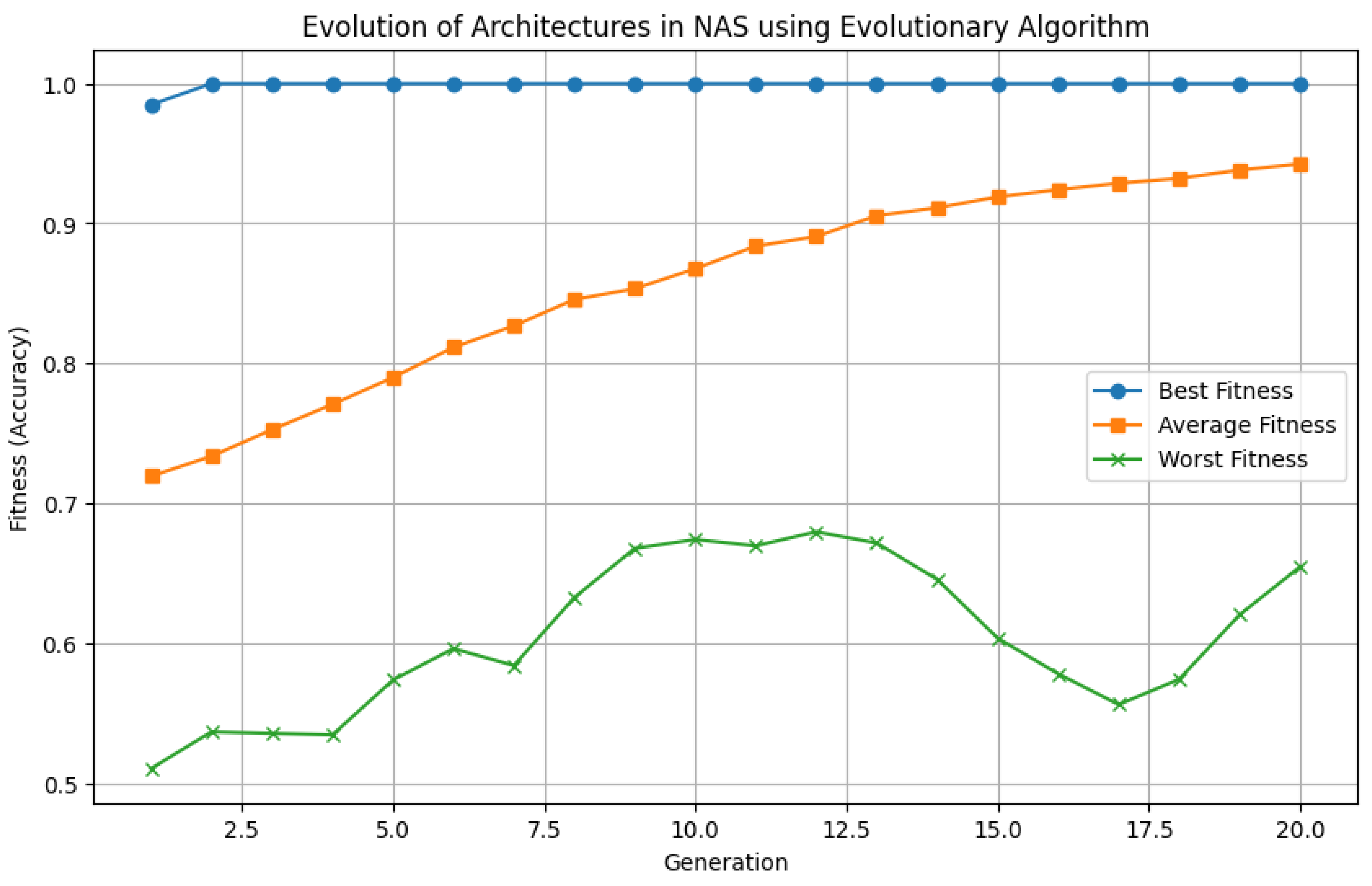
Each neural network architecture can be described by a directed acyclic graph (DAG) , where represents the set of layers (e.g., convolutional layers, pooling layers, fully connected layers), and represents the connections between them. A typical encoding scheme maps to a vector representation , where each element represents hyperparameters such as the number of filters in a convolutional layer l, kernel sizes , and activation functions . The architecture search problem can thus be formulated as an optimization problem:
where is the feasible set of architectures defined by design constraints (e.g., hardware constraints, FLOP limitations). The evolutionary process begins with the initialization of a population , where architectures are randomly generated or sampled from prior knowledge. At each generation t, a selection operator S chooses a subset of architectures based on their fitness scores:
Common selection methods include tournament selection and rank-based selection. The selected architectures undergo crossover and mutation operations. Crossover combines two parent architectures and to produce an offspring using a recombination function C:
For instance, if architectures are encoded as binary strings representing layer connections, one-point or uniform crossover can be applied:
where k is a randomly selected crossover point.
Figure 145.
Evolutionary Algorithm in Neural Architecture Search
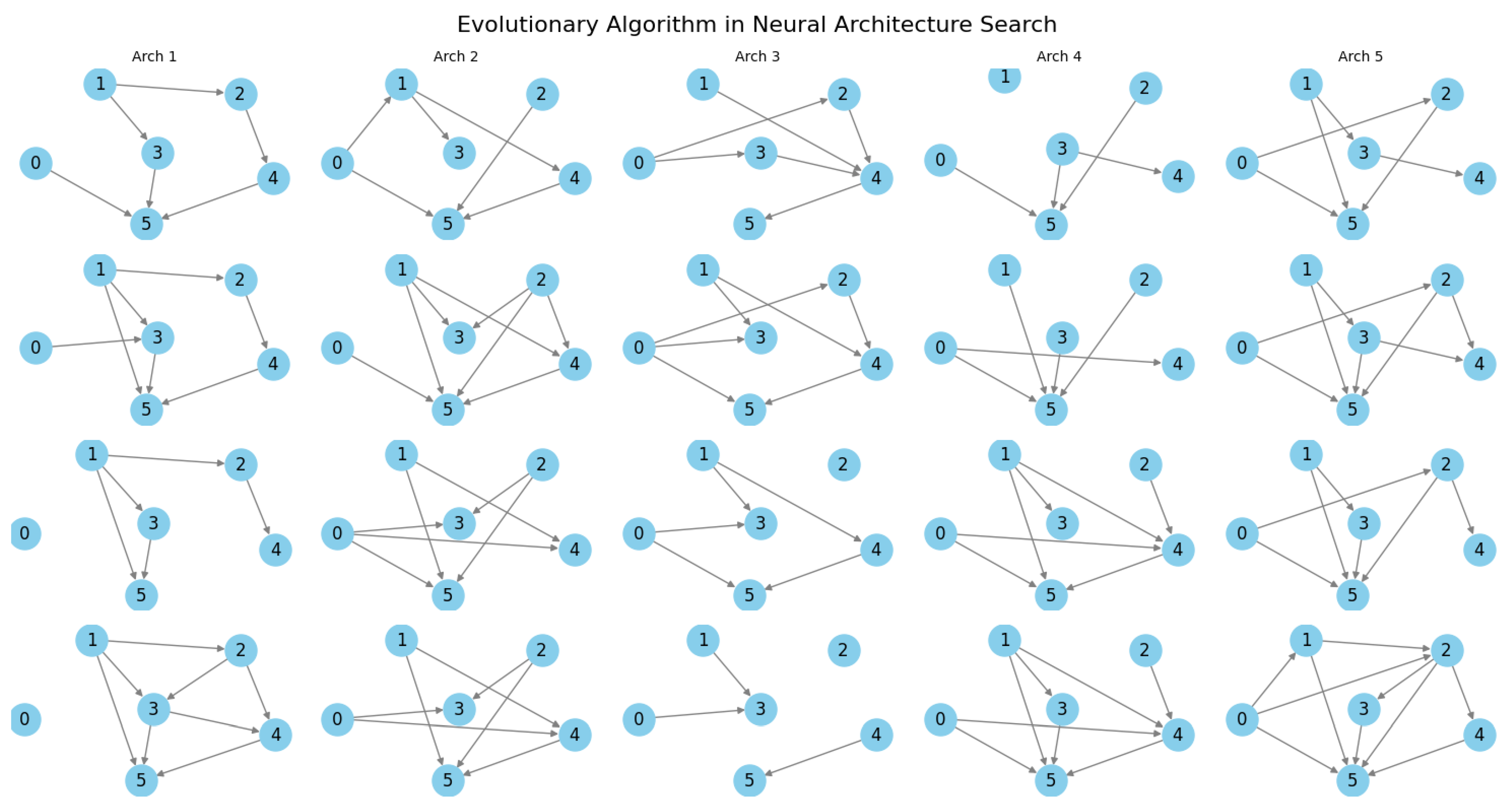
Mutation introduces random variations in the offspring architecture to maintain diversity in the population. Given a mutation rate , a mutation operator M perturbs the architecture encoding:
Common mutation operations include altering the number of filters , modifying kernel sizes , or randomly inserting/deleting layers. The updated population for the next generation is formed by selecting the top-performing architectures:
where is the set of offspring architectures and elitism ensures that the best architectures persist across generations. The process repeats until a termination criterion is met, such as a maximum number of generations T or convergence in fitness scores:
where is a predefined tolerance threshold. The search efficiency of EAs can be enhanced using surrogate models that approximate the fitness function:
where is a kernel function and are weights learned from evaluated architectures. Bayesian optimization and neural predictors are often employed to guide the search towards promising regions of . To further improve convergence speed, weight inheritance strategies transfer trained weights from parent networks to offspring, reducing the need for full training cycles. Given a parent-offspring pair , weight inheritance is expressed as:
where and denote the weight matrices of the parent and child networks, and is a transformation function that maps weights based on structural similarities. Evolutionary NAS has demonstrated competitive performance against reinforcement learning-based and gradient-based approaches, particularly in discovering novel architectures for convolutional neural networks (CNNs) and transformers. The combination of evolutionary search with differentiable search spaces, such as in Differentiable Architecture Search (DARTS), leads to hybrid methods where architectures evolve within a continuous relaxation of the search space:
where represents architecture parameters and is a softmax function ensuring differentiability. By integrating EAs with differentiable optimization, recent methods achieve state-of-the-art performance while maintaining exploration capabilities.
15.2. Reinforcement Learning in Network Architecture Search
Reinforcement Learning (RL) plays a pivotal role in Network Architecture Search (NAS) for Deep Neural Networks (DNNs) by formulating the problem as a sequential decision-making process, wherein a policy optimizes the selection of architectural components to maximize a predefined performance metric, typically validation accuracy.
Figure 146.
Reinforcement Learning in Neural Architecture Search (NAS)
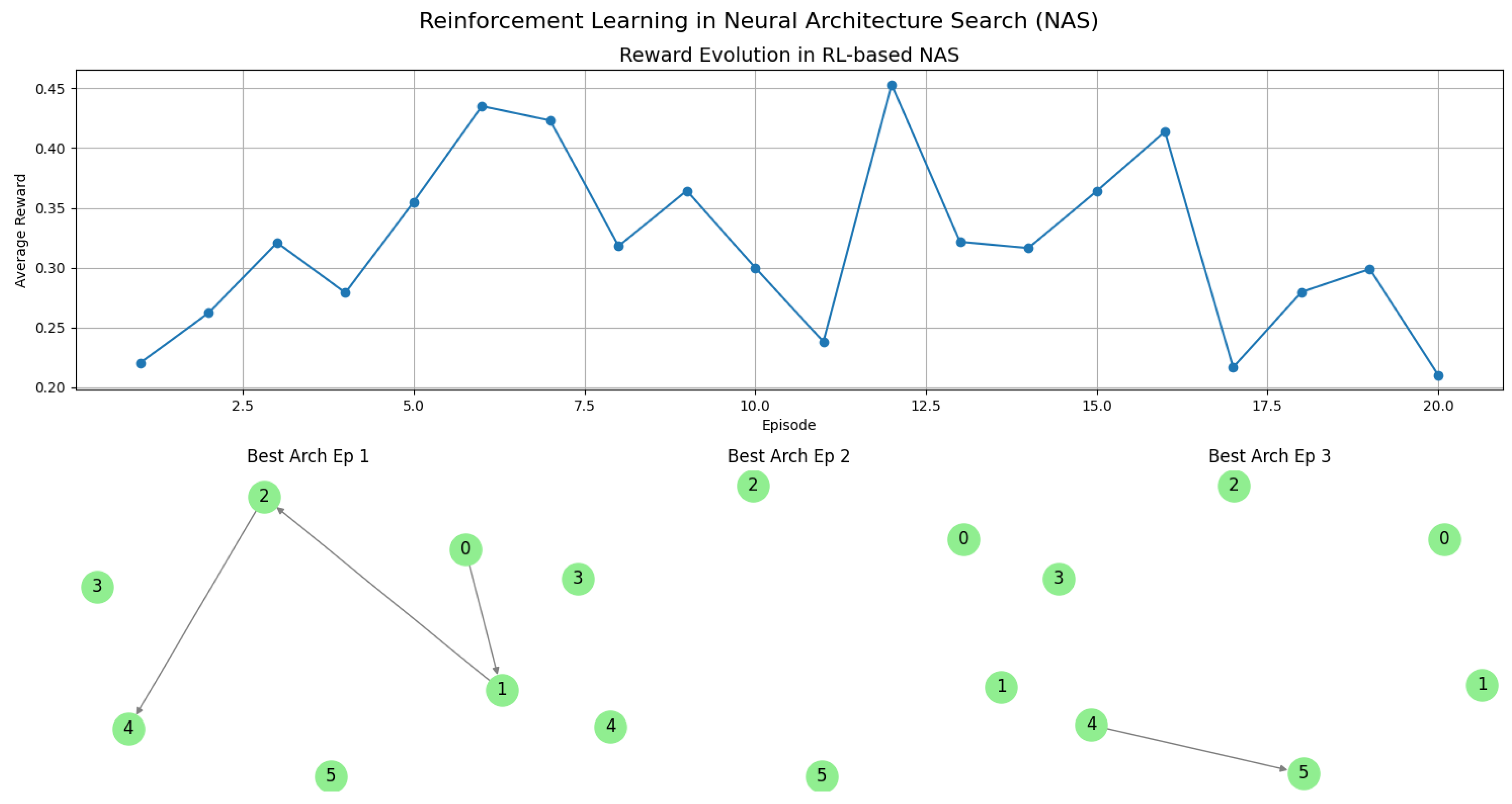
The process is modeled as a Markov Decision Process (MDP), defined by the tuple , where represents the state space corresponding to partially constructed architectures, is the action space defining possible modifications to architectures, P is the transition probability governing the evolution of architectures, R denotes the reward function that quantifies model performance, and is the discount factor controlling long-term reward contributions. The objective is to optimize the policy , parameterized by , such that the expected cumulative reward is maximized:
To optimize , policy gradient methods are employed, where the gradient of the expected reward with respect to policy parameters is given by:
Using Monte Carlo estimates, the policy parameters are updated via gradient ascent:
A common approach to implementing NAS with RL is the use of a Recurrent Neural Network (RNN)-based controller that generates candidate architectures sequentially. The hidden state of the RNN encodes information about the architecture decisions made up to step t, and the action at each step is sampled from a softmax distribution:
The reward signal is obtained by training and evaluating the generated architecture on a validation set, yielding an accuracy score A, which serves as the reward:
where b is a baseline used in variance reduction techniques such as REINFORCE. The training of the controller follows the REINFORCE algorithm with baseline subtraction:
To further stabilize learning, advantage estimation methods such as Generalized Advantage Estimation (GAE) can be employed, where the advantage function is computed using the value function :
An alternative approach is to model the NAS problem as a Q-learning task, where the Q-value represents the expected future reward given a state-action pair:
The Q-values are updated using the Bellman equation:
In practical implementations, Deep Q-Networks (DQN) are utilized, where a neural network approximates the Q-function , and updates are made using the loss function:
where represents target network parameters and D is an experience replay buffer. To address the instability of Q-learning, Double Q-learning is often employed, where two networks, and , are used to decouple action selection and evaluation:
where selects the minimum Q-value from two estimators to mitigate overestimation bias. In actor-critic methods such as Proximal Policy Optimization (PPO), the actor updates the policy while the critic evaluates its performance using the objective:
This clipped objective prevents large policy updates, ensuring stability in the RL-based NAS framework. By iteratively refining the architecture using these RL techniques, NAS can effectively discover high-performing network topologies that outperform manually designed architectures.
15.3. Policy Gradient Methods in Network Architecture Search
Policy gradient methods provide a mathematically rigorous framework for optimizing network architectures in deep neural networks by formulating the architecture search as a reinforcement learning (RL) problem. The core idea is to define a probability distribution over possible network architectures, represented as a parametric policy , where s represents the state (e.g., the current design choices or hyperparameters of the network), and a represents an action (e.g., selecting a particular layer type, activation function, or connection pattern).
Figure 147.
Policy Gradient Methods in Neural Architecture Search (NAS)
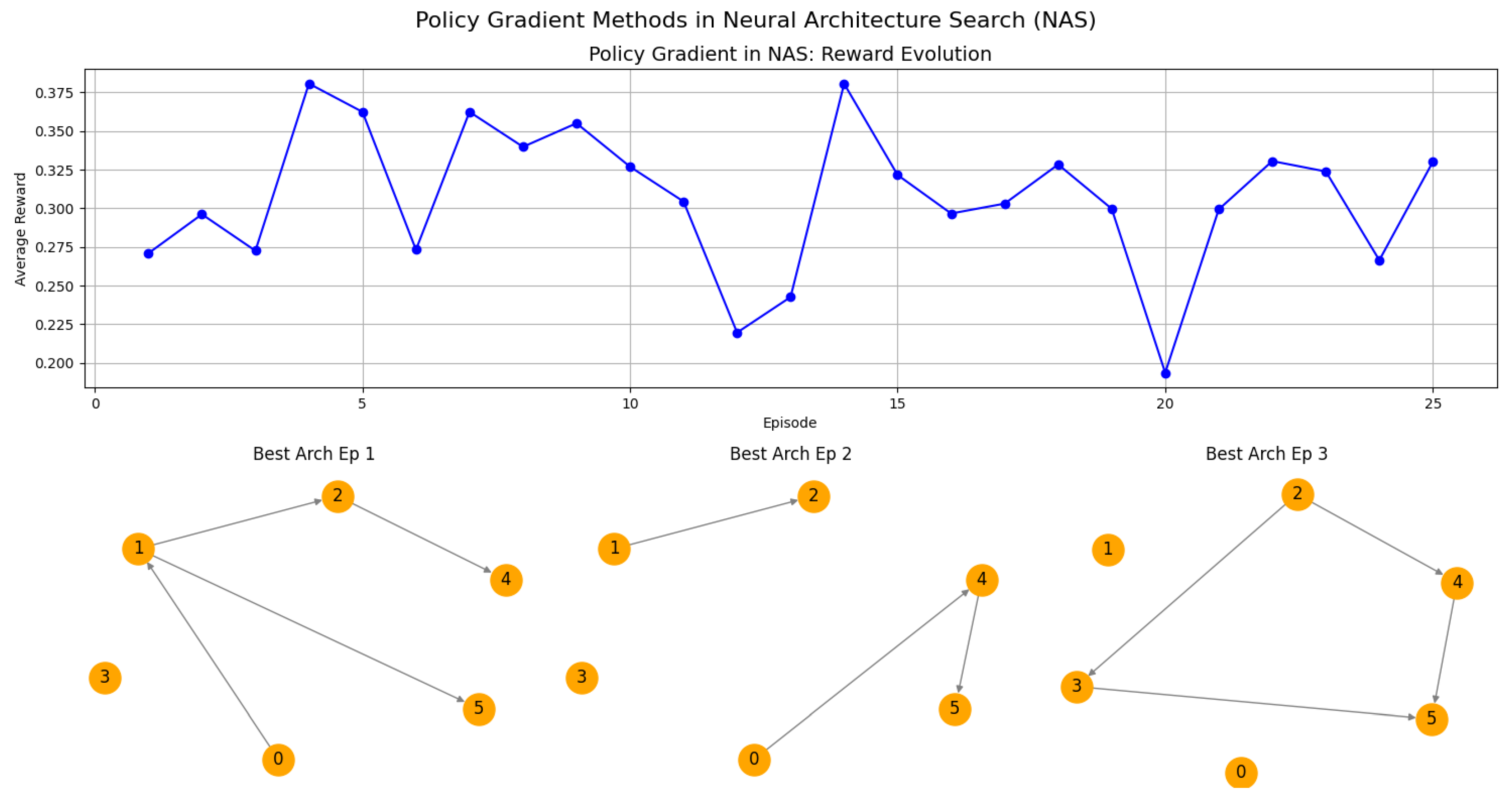
The objective is to maximize the expected performance of the architecture, which is commonly formulated as the expected reward obtained from training and evaluating the selected network:
where is a trajectory of states and actions sampled according to the policy , and represents the cumulative reward (e.g., validation accuracy of the trained architecture). The distribution over trajectories is given by
where is the environment transition function, often deterministic in the context of architecture search. To optimize , the policy gradient theorem provides an unbiased estimator of the gradient using the likelihood ratio trick:
Expanding the gradient term, we obtain
Thus, the gradient estimate simplifies to
In practice, this expectation is estimated via Monte Carlo sampling over a set of architectures, leading to the update rule:
To improve convergence, a baseline is often introduced to reduce variance:
A common choice for is a learned value function , leading to an advantage function , which forms the basis for actor-critic methods. The reward function is typically designed to reflect the generalization ability of the architecture, often incorporating the validation accuracy of the trained model:
where denotes the architecture defined by the trajectory , represents the network function, and are the trained weights obtained by minimizing the training loss
To improve exploration, entropy regularization is often added to the objective:
where
encourages diverse architecture sampling. In a real implementation, the policy is usually parameterized by a recurrent neural network (RNN) such as an LSTM, where the hidden state encodes past architecture decisions. The architecture parameters are updated using stochastic gradient descent with policy gradient updates, while the sampled architectures are trained using standard backpropagation. The convergence of policy gradient methods in architecture search relies on ensuring sufficient exploration and avoiding premature convergence to suboptimal architectures. Techniques such as proximal policy optimization (PPO), trust region policy optimization (TRPO), and natural gradient methods are often used to stabilize updates and improve sample efficiency. These methods modify the standard gradient update by introducing constraints such as
where is the Kullback-Leibler divergence, ensuring that the updated policy does not deviate too drastically from the previous policy, thereby maintaining stability in the optimization process.
15.4. Neural Tangent Kernels (NTKs) in Network Architecture Search
Neural Tangent Kernels (NTKs) have emerged as a powerful theoretical framework for understanding the training dynamics and generalization properties of deep neural networks in the infinite-width limit. In the context of Network Architecture Search (NAS), NTKs provide a mathematically rigorous way to evaluate the expressivity and trainability of different neural network architectures without explicitly training them, thereby significantly reducing computational costs associated with traditional NAS methods.
Figure 148.
NTKs, Eigenvalue Spectra, and Condition Numbers for NAS Architectures
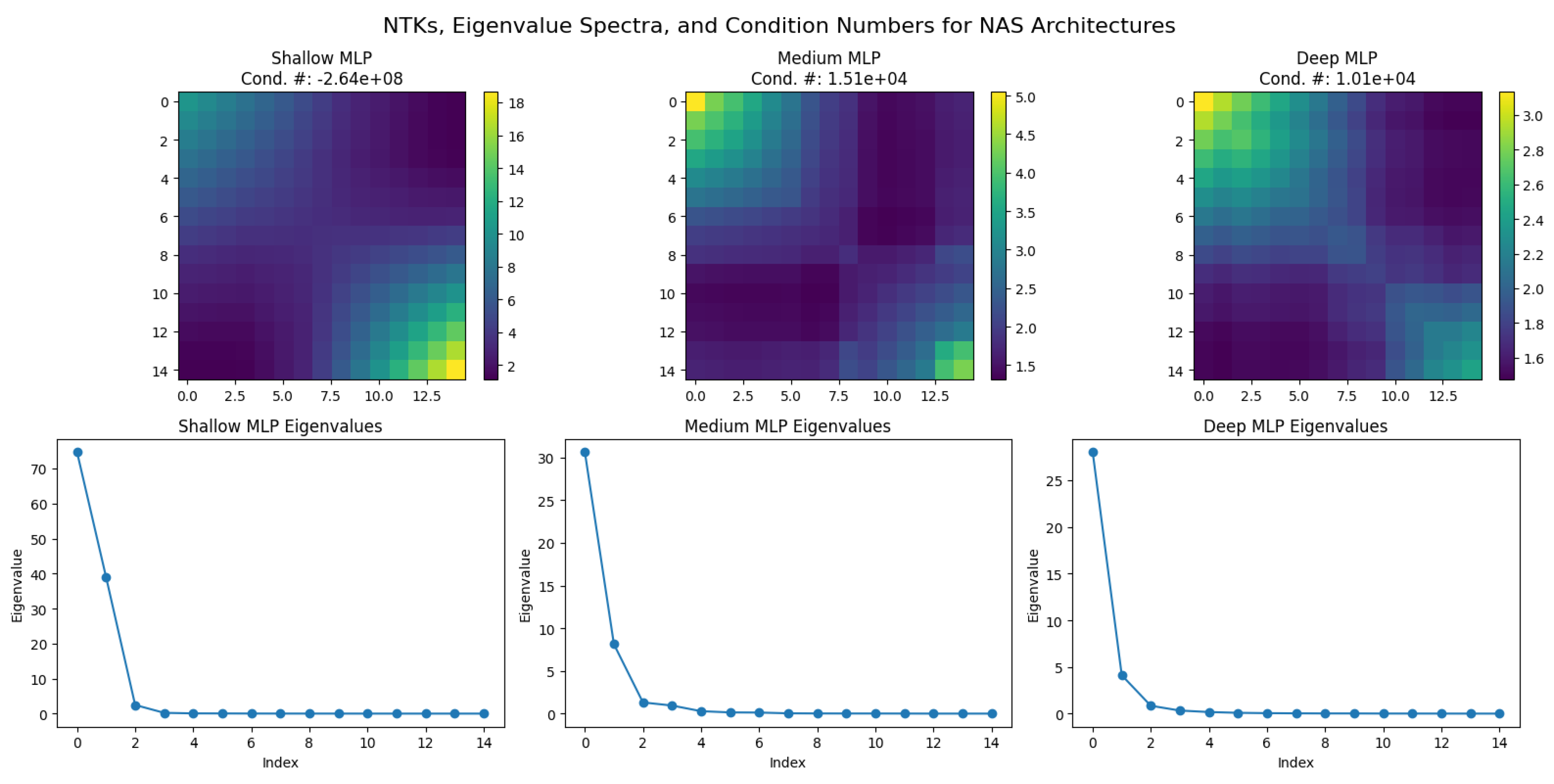
The NTK is formally defined as the Gram matrix of the Jacobian of the neural network outputs with respect to its parameters, capturing how perturbations in parameters influence the output function. Mathematically, if denotes the output of a neural network with parameters for an input x, then the NTK is given by
As the width of the network approaches infinity, the NTK remains constant during training under gradient descent, allowing the network to be effectively modeled as a Gaussian process. This property enables rapid evaluation of the convergence behavior and generalization ability of a given architecture by analyzing the eigenvalues of the NTK matrix. The training dynamics of an infinitely wide neural network can be described using the evolution of the function under gradient descent with a learning rate , which follows
Since the NTK remains constant in the infinite-width regime, this equation can be solved explicitly using
where denotes the training set inputs, and are the corresponding targets. The rate of convergence is determined by the smallest eigenvalue of , implying that architectures with larger minimum eigenvalues of their NTKs converge faster and are thus more trainable. The NTK perspective enables a principled approach to NAS by evaluating candidate architectures based on their kernel spectra, particularly the condition number , which governs the stability of gradient descent. Generalization in deep learning is often characterized by the smoothness and complexity of learned functions. The NTK controls the function space induced by a given architecture, allowing estimation of generalization error through the kernel ridge regression formula
where is the noise variance. Architectures with better generalization properties exhibit smaller trace norms of the NTK inverse.
Figure 149.
CNN NTKs and Eigenvalue Spectra for NAS Architectures
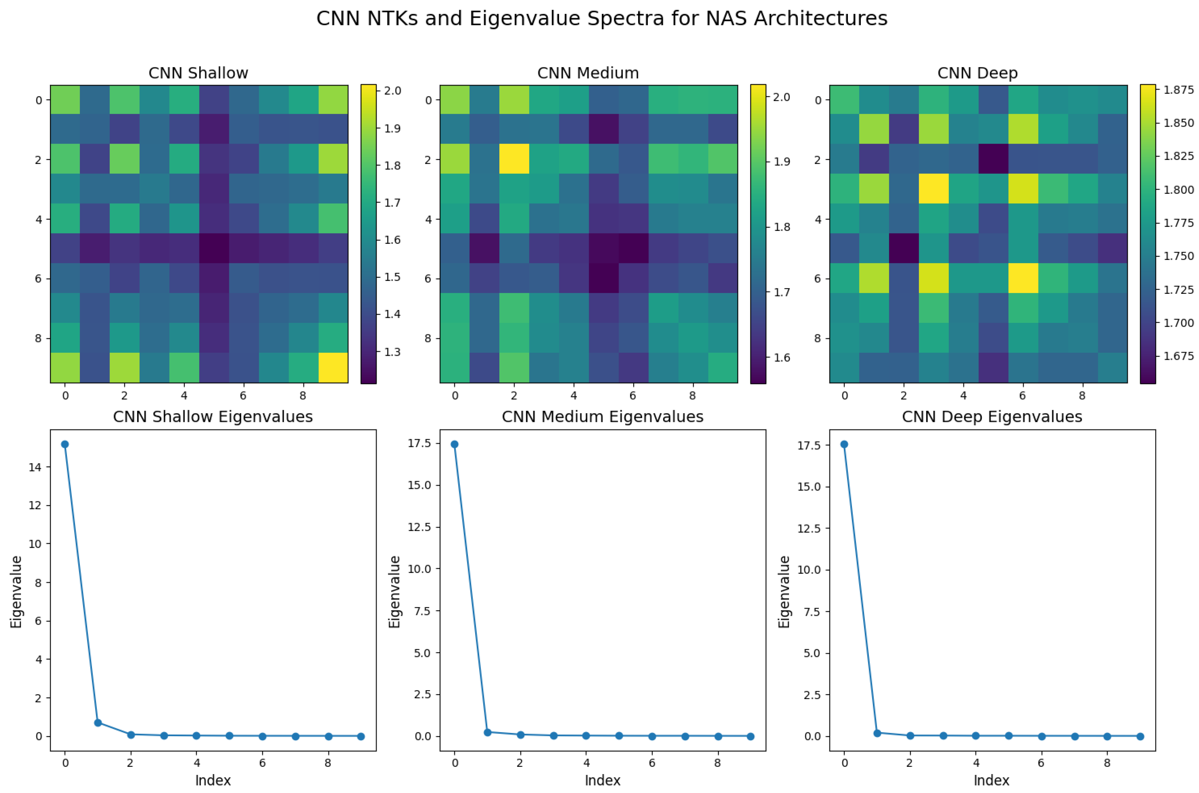
In the infinite-width limit, NTKs of different architectures can be computed analytically by considering the recursive propagation of covariance matrices through network layers. For a fully connected network with ReLU activation, the NTK at depth L is given by
where is the derivative of the activation function’s covariance kernel. Different architectures, such as convolutional neural networks (CNNs), modify this recurrence relation by incorporating weight-sharing and local connectivity constraints. The NTK for a CNN layer with filter size k is
This allows NAS to be performed analytically by evaluating how architectural choices influence the NTK and its spectral properties, bypassing the need for expensive training runs. Recent work has extended NTK-based NAS to attention-based architectures, such as transformers, where the self-attention mechanism induces a structured NTK
where are the query, key, and value matrices. The spectrum of determines the expressivity and trainability of transformer-based models, enabling NTK-based architectural optimization in sequence learning tasks. The NTK framework provides an elegant, mathematically rigorous approach to NAS by linking architectural choices to trainability and generalization through spectral analysis of the kernel.
16. Learning Paradigms
16.1. Unsupervised Learning
16.1.1. Literature Review of Unsupervised Learning
Unsupervised learning has evolved significantly through foundational contributions in clustering, probabilistic modeling, neural representations, and generative techniques. One of the earliest and most fundamental methods in clustering was introduced by MacQueen in 1967 [1035] with the k-means algorithm. This algorithm partitions a set of n observations into k clusters in such a way that the intra-cluster variance is minimized. The iterative nature of k-means, involving cluster centroid updates and reassignment of points based on their Euclidean distances, remains a cornerstone of clustering techniques. Complementing k-means, the Expectation-Maximization (EM) algorithm, rigorously formalized by Dempster, Laird, and Rubin in 1977 [1036] provided a general framework for maximizing likelihood estimates in models with latent variables. EM underpins Gaussian Mixture Models (GMMs), allowing for probabilistic clustering by modeling data as a weighted sum of Gaussian distributions. These models account for uncertainty and have led to advancements in density estimation and soft clustering.
Another major breakthrough in unsupervised learning emerged with the self-organizing maps (SOMs) developed by Kohonen in 1982 [1037]. These neural-inspired models provide a competitive learning framework where neurons adjust their weights to form low-dimensional representations of input data while preserving topological relationships. This biologically motivated approach to clustering has been instrumental in feature extraction and visualization, especially in applications involving high-dimensional data. Parallel to SOMs, spectral techniques for manifold learning and dimensionality reduction were rigorously developed, with Belkin and Niyogi [1038] introducing Laplacian Eigenmaps in 2003. This method constructs a graph Laplacian to capture local geometric properties of data manifolds and embed them into a lower-dimensional space while maintaining neighborhood relationships. This has provided a mathematically principled foundation for spectral clustering and nonlinear dimensionality reduction.
The rigorous treatment of information-theoretic principles in unsupervised learning was significantly advanced by the Information Bottleneck (IB) method proposed by Tishby, Pereira, and Bialek in 2000 [1039]. The IB principle establishes a trade-off between compression and predictive efficiency by optimizing a mutual information objective. This formulation has deeply influenced representation learning, particularly in autoencoders and deep latent variable models. A major advancement in unsupervised neural representations was introduced by Hinton and Salakhutdinov in 2006 [1040], demonstrating that deep belief networks (DBNs) could learn hierarchical representations via layer-wise training of restricted Boltzmann machines (RBMs). This work laid the foundation for the resurgence of deep learning by showing that unsupervised pretraining significantly improves the performance of neural networks. The probabilistic formulation of deep unsupervised learning was further developed by Kingma and Welling in 2013 [1041] with the introduction of variational autoencoders (VAEs). By leveraging variational inference, VAEs provide a rigorous framework for learning latent variable models, enabling efficient probabilistic generative modeling of complex data distributions.
A more adversarial approach to generative modeling was pioneered by Goodfellow et al. in 2020 [121] with the introduction of generative adversarial networks (GANs). GANs consist of a generator and discriminator competing in a minimax game, where the generator learns to produce realistic samples while the discriminator improves its ability to distinguish between real and generated data. This adversarial framework has profoundly impacted image generation, domain adaptation, and semi-supervised learning by producing high-quality synthetic data. The visualization of high-dimensional data was further enhanced by van der Maaten and Hinton in 2008 [1042] with the development of t-distributed stochastic neighbor embedding (t-SNE). This method provides a probabilistic approach to mapping data points into a lower-dimensional space by minimizing the Kullback-Leibler divergence between high- and low-dimensional distributions, preserving local similarities. t-SNE has become a widely used technique in exploratory data analysis due to its ability to reveal meaningful structure in complex datasets.
Together, these contributions have shaped the field of unsupervised learning by introducing rigorous mathematical formulations for clustering, probabilistic modeling, and representation learning. The foundational algorithms such as k-means and EM provide essential tools for unsupervised data analysis, while information-theoretic and spectral methods offer deeper insights into structure preservation and feature extraction. The integration of neural networks into unsupervised learning, through self-organizing maps, deep belief networks, and variational autoencoders, has led to a significant expansion in the capabilities of machine learning models. The development of adversarial training with GANs and the application of information bottleneck principles further illustrate the growing sophistication of unsupervised learning techniques. These advancements continue to push the boundaries of artificial intelligence, enabling models to learn rich, structured representations of data without the need for explicit supervision.
Roweis and Saul (2000) [1043] introduced Locally Linear Embedding (LLE), a nonlinear dimensionality reduction algorithm designed to uncover low-dimensional structures within high-dimensional data. The core idea behind LLE is to preserve the local geometric relationships between neighboring data points while embedding them into a lower-dimensional space. Unlike linear techniques such as Principal Component Analysis (PCA), which assume that the global structure of the data can be well represented using a linear subspace, LLE focuses on preserving the local structure by considering each data point and its nearest neighbors. The algorithm operates in three main steps. First, for each data point, LLE identifies a set of nearest neighbors based on a distance metric, usually Euclidean distance. Second, it computes local reconstruction weights by expressing each data point as a linear combination of its neighbors, minimizing the reconstruction error while enforcing the constraint that the weights sum to one. This step ensures that the local geometric structure is encoded in an invariant manner. Third, LLE determines a lower-dimensional embedding by finding a new set of coordinates that best preserves the reconstruction weights obtained in the previous step. This is achieved by minimizing a quadratic cost function that ensures the lower-dimensional representation maintains the same local linear relationships as the original high-dimensional data. The main advantage of LLE over traditional linear techniques is its ability to recover nonlinear manifolds, making it particularly effective for data sets where the underlying structure is curved or highly nonlinear. Unlike methods such as Multidimensional Scaling (MDS), which rely on pairwise distances between all points and can be computationally expensive, LLE leverages only local neighborhoods, making it more scalable to larger data sets. Additionally, since LLE does not impose any parametric assumptions on the manifold, it is capable of adapting to a wide variety of data distributions.
However, LLE also has some limitations. Its reliance on nearest-neighbor selection makes it sensitive to noise and parameter choices, particularly the number of neighbors. Furthermore, the embeddings produced by LLE are often unnormalized, meaning that distances in the lower-dimensional space may not have a straightforward interpretation. Despite these challenges, LLE has had a significant impact on machine learning and data visualization, providing a powerful tool for uncovering the intrinsic structure of high-dimensional data in applications ranging from image processing to bioinformatics. Its introduction marked a shift toward more flexible, geometry-preserving dimensionality reduction techniques, influencing the development of subsequent manifold learning methods such as Isomap and t-SNE.
Table 10.
Summary of Contributions to the Unsupervised Learning
| Authors (Year) | Contribution |
|---|---|
| MacQueen (1967) [1035] | Introduced the k-means algorithm, a foundational clustering method that minimizes intra-cluster variance through iterative centroid updates and point reassignment based on Euclidean distance. |
| Dempster, Laird, and Rubin (1977) [1036] | Developed the Expectation-Maximization (EM) algorithm, a general framework for maximizing likelihood estimates in models with latent variables, forming the basis for Gaussian Mixture Models (GMMs). |
| Kohonen (1982) [1037] | Proposed self-organizing maps (SOMs), a neural-inspired model for competitive learning, which preserves topological relationships and has been instrumental in feature extraction. |
| Belkin and Niyogi (2003) [1038] | Introduced Laplacian Eigenmaps, which use a graph Laplacian to capture local geometric properties of data manifolds, providing a foundation for spectral clustering and nonlinear dimensionality reduction. |
| Tishby, Pereira, and Bialek (2000) [1039] | Proposed the Information Bottleneck (IB) method, optimizing mutual information to balance compression and predictive efficiency, influencing representation learning in autoencoders. |
| Hinton and Salakhutdinov (2006) [1040] | Demonstrated deep belief networks (DBNs), where layer-wise training of restricted Boltzmann machines (RBMs) enables hierarchical unsupervised representation learning. |
| Kingma and Welling (2013) [1041] | Developed variational autoencoders (VAEs), leveraging variational inference for probabilistic generative modeling of complex data distributions. |
| Goodfellow et al. (2020) [121] | Introduced generative adversarial networks (GANs), an adversarial framework where a generator and discriminator compete, leading to advances in synthetic data generation. |
| van der Maaten and Hinton (2008) [1042] | Developed t-distributed stochastic neighbor embedding (t-SNE), a probabilistic approach for high-dimensional data visualization that preserves local similarities. |
| Roweis and Saul (2000) [1043] | Introduced Locally Linear Embedding (LLE), a nonlinear dimensionality reduction technique that preserves local geometric relationships and is effective for manifold learning. |
| Bell and Sejnowski (1995) [1044] | Developed Independent Component Analysis (ICA), an information-theoretic method for blind source separation, leveraging higher-order statistics to extract statistically independent signals. |
Bell and Sejnowski (1995) [1044] introduced Independent Component Analysis (ICA) as an information-theoretic approach to blind source separation (BSS), which allows for the decomposition of mixed signals into statistically independent components without prior knowledge of the mixing process. Their work was motivated by real-world scenarios where multiple signals, such as different voices in a crowded room or overlapping audio sources in a recording, become mixed together, making it difficult to recover the original sources. Unlike traditional statistical methods such as Principal Component Analysis (PCA), which rely on second-order statistics and assume orthogonality of components, ICA leverages higher-order statistical properties to separate signals that are non-Gaussian and statistically independent. The fundamental principle behind their method is the maximization of information transfer in a neural network, also known as the infomax principle. This principle is based on the idea that a system should be optimized to maximize the mutual information between its input and output, ensuring that the output representation is as statistically independent as possible. To achieve this, they formulated a neural learning rule that iteratively adjusts the network’s weight parameters using a nonlinear function, which enhances the separation of independent sources. The key insight was that statistical independence implies that the joint probability distribution of the recovered signals should factorize into the product of their individual distributions, which is not the case for mixtures of dependent signals. To enforce this independence, their method used a contrast function derived from information theory, ensuring that the recovered sources were as non-Gaussian as possible, since mixtures of independent sources tend to become more Gaussian due to the Central Limit Theorem. This approach enabled the successful separation of mixed signals in a variety of applications, including audio processing, biomedical signal analysis, and image processing. One of the most famous demonstrations of ICA, often referred to as the “cocktail party problem,” involves separating multiple overlapping speech signals recorded by different microphones. Their algorithm was able to recover individual voices from the mixed recording with remarkable accuracy, highlighting the effectiveness of ICA in practical scenarios. Additionally, ICA found significant applications in neuroscience, particularly in electroencephalography (EEG) and functional magnetic resonance imaging (fMRI), where it helped isolate meaningful brain activity patterns from background noise.
Despite its power, ICA has limitations, including its sensitivity to the choice of nonlinear functions and the assumption that the number of independent sources does not exceed the number of observed mixtures. Furthermore, ICA assumes that the sources are statistically independent, which may not always hold in real-world data. Nonetheless, Bell and Sejnowski’s work laid the foundation for subsequent advancements in unsupervised learning, influencing modern approaches in deep learning, signal processing, and latent variable modeling. Their method provided a robust mathematical framework for data decomposition that has since been expanded and refined in numerous fields, demonstrating the lasting impact of their contribution to unsupervised learning.
16.1.2. Recent Literature Review of Unsupervised Learning
Unsupervised learning has emerged as a powerful tool in various domains, offering novel solutions where labeled data is scarce or unavailable. In semiconductor manufacturing, Parmar (2020) [1045] introduced an unsupervised learning framework aimed at identifying previously unknown defects. By leveraging clustering techniques and anomaly detection, this approach enhances quality control without relying on predefined defect categories. The ability to discover novel defect patterns autonomously makes this method particularly valuable in industries where manufacturing processes constantly evolve, and new defect types emerge. In a related field, Raikwar and Gupta (2025) [1046] developed an AI-driven trust management framework for wireless ad hoc networks. This system integrates unsupervised and supervised learning to classify network nodes based on trustworthiness, helping identify potentially malicious nodes. Such frameworks are critical in decentralized environments where security threats are unpredictable and dynamically evolving. The application of unsupervised learning in this context reduces reliance on predefined attack signatures, improving network security in real-time.
Structural health monitoring has also benefited from unsupervised learning techniques. Moustakidis et al. (2025) [1047] proposed a deep learning autoencoder framework for fast Fourier transform (FFT)-based clustering, designed to analyze acoustic emission data from composite materials. This method enables automatic detection of structural damage over time, allowing for proactive maintenance and risk mitigation in infrastructure management. By employing autoencoders to extract meaningful features from raw sensor data, the approach outperforms traditional inspection methods that require extensive manual interpretation. Feature selection is another area where unsupervised learning has made a significant impact. Liu et al. (2025) [1048] introduced an unsupervised feature selection algorithm using L2, p-norm feature reconstruction. This method effectively reduces redundant features while preserving essential data structures, thereby improving the efficiency and accuracy of clustering algorithms. High-dimensional datasets, such as those used in bioinformatics and financial modeling, greatly benefit from this technique, as it enables better data representation and pattern discovery without the need for labeled guidance.
In the medical and healthcare sector, unsupervised learning has been leveraged for disease risk assessment and biomarker discovery. Zhou et al. (2025) [1049] applied clustering techniques to analyze metabolic profiles, uncovering hidden subtypes of hypertriglyceridemia associated with varying disease risks. This research demonstrates the potential of unsupervised learning in personalized medicine, where identifying metabolic subgroups can help tailor treatments to individual patients rather than applying a one-size-fits-all approach. Similarly, Lin et al. (2025) [1050] employed unsupervised learning for risk control in health insurance fund management. By analyzing claims data and identifying anomalous patterns, this approach enhances fraud detection and risk assessment, ultimately leading to better resource allocation and cost reduction. The ability to detect fraud without labeled examples is a significant advantage in an industry where fraudulent activities are often sophisticated and constantly evolving.
Beyond healthcare, unsupervised learning has shown promise in improving real-world object detection systems. Huang et al. (2025) [1051] proposed a novel unsupervised domain adaptation technique to enhance open-world object detection. Unlike traditional supervised models that require large amounts of labeled data, this approach enables object detection models to generalize across different environments with minimal supervision. Such advancements are crucial in autonomous navigation, surveillance, and robotics, where training data may not always be representative of real-world conditions. In a different engineering application, Wu and Liu (2025) [1052] introduced a VQ-VAE-2-based algorithm for detecting cracks in concrete structures. This unsupervised approach automates structural health monitoring, reducing dependence on costly manual inspections while improving the accuracy and efficiency of damage assessments.
Natural language processing and medical imaging have also seen substantial contributions from unsupervised learning. Nagelli and Saleena (2025) [1053] developed an aspect-based sentiment analysis model using self-attention mechanisms. This model enables the automatic extraction of sentiment-related features from multilingual datasets, allowing businesses to analyze customer feedback without requiring labeled sentiment data. Such models are essential for real-time sentiment analysis in global markets where user-generated content is vast and diverse. Meanwhile, Ekanayake (2025) [1054] applied deep learning techniques for MRI reconstruction and super-resolution enhancement. This research significantly reduces MRI scan times while preserving high image quality, offering a transformative solution to the challenges of medical imaging. The use of unsupervised learning in this context enables more efficient data-driven reconstruction techniques, reducing dependency on expensive and time-consuming manually labeled training datasets. These diverse applications illustrate the expanding role of unsupervised learning in solving complex real-world problems, demonstrating its adaptability and potential to drive further innovation across multiple industries.
Table 11.
Summary of Recent Contributions in Unsupervised Learning
| Authors (Year) | Contribution |
|---|---|
| Parmar (2025) [1045] | Introduced an unsupervised learning framework for identifying unknown defects in semiconductor manufacturing, leveraging clustering and anomaly detection to improve quality control in industrial settings. |
| Raikwar and Gupta (2025) [1046] | Developed an AI-driven trust management framework for wireless ad hoc networks, combining unsupervised and supervised learning to classify network nodes based on trustworthiness and detect malicious activity. |
| Moustakidis et al. (2025) [1047] | Proposed deep learning autoencoders for FFT-based clustering in structural health monitoring, enabling automated detection of temporal damage evolution in composite materials. |
| Liu et al. (2025) [1048] | Designed an unsupervised feature selection algorithm using L2, p-norm feature reconstruction, reducing redundant features and improving clustering performance for high-dimensional datasets. |
| Zhou et al. (2025) [1049] | Applied unsupervised clustering techniques to metabolic profiles, identifying hidden metabolic subtypes associated with hypertriglyceridemia and disease risks, advancing personalized medicine. |
| Lin et al. (2025) [1050] | Developed an unsupervised learning-based risk control model for health insurance fund management, effectively identifying high-risk groups and fraudulent claims through anomaly detection. |
| Huang et al. (2025) [1051] | Proposed an unsupervised domain adaptation method for open-world object detection, enabling models to generalize across different environments without extensive labeled datasets. |
| Wu and Liu (2025) [1052] | Designed a VQ-VAE-2-based unsupervised detection algorithm for concrete crack identification, automating structural health monitoring and reducing manual inspection efforts. |
| Nagelli and Saleena (2025) [1053] | Developed an aspect-based sentiment analysis model using self-attention mechanisms, enabling multilingual sentiment analysis without labeled training data. |
| Ekanayake (2025) [1054] | Applied deep learning-based unsupervised learning for MRI reconstruction and super-resolution, reducing scan times while maintaining high image quality in medical imaging. |
16.1.3. Mathematical Analysis of Unsupervised Learning
Unsupervised learning is a fundamental paradigm in machine learning, in which a model is trained on a dataset without explicit supervision in the form of labeled outputs. Mathematically, given a dataset consisting of N data points, where each is a vector in , the goal is to find an underlying structure, distribution, or latent representation of the data, often formulated as a function where k may be lower than d, capturing essential properties of the data manifold. The data is assumed to be drawn from an unknown probability distribution , and the central objective in unsupervised learning is to model or approximate this distribution using a function , where represents the parameters of the model. This can be done using probabilistic modeling, clustering, dimensionality reduction, and manifold learning.
One of the most rigorous formulations in unsupervised learning arises in the estimation of probability density functions, where the likelihood function of the observed data is given by
The optimal parameters are obtained by maximizing the log-likelihood function:
In clustering problems, an objective function is often defined to minimize intra-cluster variance while maximizing inter-cluster separation. Given a set of K cluster centers , the assignment of each point to a cluster is determined by
The objective function to minimize is given by
Expectation-Maximization (EM) algorithms generalize clustering in a probabilistic framework, where data is assumed to be generated by a mixture of distributions:
where are the mixture weights such that , and are component distributions, often taken as Gaussian:
Dimensionality reduction techniques such as Principal Component Analysis (PCA) seek to find a lower-dimensional representation that maximizes variance. Given a centered data matrix , PCA finds the eigenvectors of the covariance matrix
The principal components are obtained by solving the eigenvalue problem
Only the top k eigenvectors corresponding to the largest eigenvalues are retained, reducing the data to a lower-dimensional subspace. The transformation to the new basis is given by
where V is the matrix of top eigenvectors. More advanced methods such as autoencoders learn a mapping from input data to a latent representation using an encoder function
and reconstruct the input via a decoder function
The reconstruction loss is typically measured as
For probabilistic models, Variational Autoencoders (VAEs) extend autoencoders by introducing a latent variable model with a prior distribution , an approximate posterior , and a reconstruction likelihood . The objective function in VAEs is to maximize the evidence lower bound (ELBO):
where is the Kullback-Leibler divergence. Generative models such as Generative Adversarial Networks (GANs) learn a mapping from a simple latent space to the data distribution via a generator function , while an adversarial discriminator D learns to distinguish between real and generated samples. The objective function of a GAN is given by
16.1.4. Information Bottleneck (IB) Method
16.1.4.1 Literature Review of Information Bottleneck (IB) Method
The Information Bottleneck (IB) method, introduced by Tishby, Pereira, and Bialek (1999) [1068], provides a principled approach to extracting relevant information from a random variable X concerning another variable Y. The method formulates an optimization problem that seeks to find a compressed representation T of X that retains the maximal information about Y, while minimizing the redundancy in X. This is achieved by balancing the mutual information terms and , where a Lagrange multiplier controls the trade-off between compression and relevance. The authors derived an iterative algorithm based on variational principles to solve this optimization problem and demonstrated its utility in clustering and data representation tasks. This work laid the foundation for a vast array of subsequent research efforts that have expanded the scope of the IB method to different domains and problem settings, providing deeper insights into the nature of information-theoretic compression and representation learning.
One of the key extensions of the IB method was its application to continuous-valued variables, particularly those following a Gaussian distribution. Chechik, Globerson, Tishby, and Weiss (2005) [1069] rigorously examined the IB method in the context of jointly Gaussian random variables, deriving analytical solutions that revealed the intrinsic connections between the IB formulation and classical techniques such as canonical correlation analysis. Their results demonstrated that the optimal representation in the Gaussian case can be expressed in terms of principal component analysis (PCA)-like transformations, thereby bridging the IB method with traditional dimensionality reduction approaches. This work has had significant implications for signal processing and statistical learning, as it provides a mathematically rigorous foundation for applying the IB principle to real-world datasets that exhibit Gaussian-like characteristics. In a related extension, Chechik and Tishby (2002) [1070] introduced a variant of the IB framework that incorporates side information, allowing for the extraction of representations that retain information about one target variable while being uninformative about another. This formulation has proven particularly useful in privacy-preserving machine learning and fairness-aware representations, where one seeks to ensure that a learned representation encodes task-relevant information while obfuscating sensitive attributes.
In the context of deep learning, Tishby and Zaslavsky (2015) [1071] proposed that the training process of deep neural networks (DNNs) can be interpreted through the lens of the IB principle. They hypothesized that DNNs undergo two distinct phases during training: an initial "fitting" phase where the mutual information between successive layers and the target variable Y increases, followed by a "compression" phase where the network progressively reduces the mutual information between intermediate layers and the input variable X. This perspective provides a theoretical justification for why deep networks generalize well despite their over-parameterization, as the compression phase effectively filters out irrelevant variations in the input while preserving task-relevant features. However, Saxe et. al. (2019) [1072] critically examined this hypothesis and argued that the presence of the compression phase is highly dependent on architectural choices, particularly the activation functions used in deep networks. Their empirical findings demonstrated that the IB theory does not universally apply to all neural network architectures, suggesting that while information-theoretic compression may play a role in some settings, it is not a fundamental principle governing the training dynamics of all deep networks.
Further empirical support for the IB perspective in deep learning was provided by Shwartz-Ziv and Tishby (2017) [1073], who conducted a detailed analysis of information flow in deep neural networks. Using information plane visualizations, they showed that the training process of DNNs aligns with the two-phase description proposed in earlier work. Their findings provided strong evidence for the compression phenomenon in networks trained with stochastic gradient descent (SGD), reinforcing the argument that deep networks learn compact representations of the input. However, a major challenge in applying the IB framework to high-dimensional data is the difficulty of accurately estimating mutual information, especially in deep networks where the latent representations are highly non-Gaussian. To address this issue, Noshad et. al. (2019) [1074] introduced a novel mutual information estimator based on dependence graphs, enabling more scalable and robust estimations of information flow in deep learning models. Their approach has opened new avenues for applying the IB principle to real-world machine learning problems where traditional mutual information estimators fail due to the curse of dimensionality.
The theoretical implications of information bottleneck in neural networks were further explored by Goldfeld et. al. (2018) [1075], who developed refined techniques for estimating mutual information in deep networks. Their work provided new tools for analyzing the role of compression in neural representations, offering rigorous mathematical justifications for why certain layers in deep networks tend to exhibit strong compression effects. More recently, Geiger (2021) [1077] presented a comprehensive review of information plane analyses in neural network classifiers, evaluating the strengths and limitations of the IB framework in this setting. His analysis raised critical questions about the general applicability of IB-based insights in deep learning, highlighting cases where the information plane approach fails to provide accurate characterizations of training dynamics. Building on these theoretical developments, Kawaguchi, Deng, Ji, and Huang (2023) [1078] rigorously analyzed the generalization properties of neural networks under the IB framework, providing a mathematical link between information compression and generalization error bounds. Their results establish that controlling the information bottleneck can serve as a regularization mechanism, leading to improved generalization performance in deep learning models. Collectively, these contributions underscore the profound impact of the IB principle across a wide range of disciplines, from statistical signal processing to modern artificial intelligence.
| Authors (Year) | Contribution |
| Tishby et al. (1999) [1068] | Introduced the Information Bottleneck (IB) method, formulating an optimization problem that balances mutual information terms to extract relevant information from a random variable while minimizing redundancy. Developed an iterative variational algorithm for solving the IB problem, demonstrating its application in clustering and representation learning. |
| Chechik et al. (2003) [1069] | Extended the IB method to jointly Gaussian variables, deriving analytical solutions that connect IB with canonical correlation analysis and PCA. Provided a rigorous foundation for applying IB to real-world Gaussian data. |
| Chechik and Tishby (2002) [1070] | Developed a variant of the IB framework incorporating side information, enabling extraction of representations that retain information about one target while obfuscating another. Applied to privacy-preserving and fairness-aware machine learning. |
| Tishby and Zaslavsky (2015) [1071] | Proposed that deep neural network training follows an IB perspective, consisting of an initial fitting phase followed by a compression phase, explaining generalization through information-theoretic principles. |
| Saxe et al. (2019) [1072] | Critically examined the IB hypothesis in deep learning, showing that the presence of a compression phase depends on network architecture and activation functions, challenging the universality of IB in training dynamics. |
| Shwartz-Ziv and Tishby (2017) [1073] | Conducted empirical analysis of information flow in deep networks using information plane visualizations, providing evidence for compression in networks trained with SGD and reinforcing IB-based interpretations. |
| Noshad et al. (2019) [1074] | Developed a new mutual information estimator using dependence graphs to improve the scalability and accuracy of IB-based analyses in high-dimensional settings, addressing limitations of traditional estimators. |
| Goldfeld et al. (2018) [1075] | Provided refined mutual information estimation techniques for deep networks, offering rigorous mathematical justifications for compression effects in neural representations. |
| Geiger (2021) [1077] | Reviewed information plane analyses in neural classifiers, evaluating the strengths and weaknesses of IB interpretations, highlighting cases where IB fails to accurately characterize training dynamics. |
| Kawaguchi et al. (2023) [1078] | Analyzed generalization properties of neural networks under IB, linking information compression to generalization error bounds and establishing IB as a regularization mechanism for improved performance. |
16.1.4.2 Recent Literature Review of Information Bottleneck (IB) Method
The Information Bottleneck (IB) method has been widely applied across various disciplines, contributing significantly to fields such as machine learning, reinforcement learning, adversarial robustness, plant metabolomics, and quantum computing. One of the most notable contributions comes from Dardour et al. (2025) [1079], who introduced a novel approach to enhance adversarial robustness in stochastic neural networks. By leveraging inter-separability and intra-concentration, their study demonstrated that using the IB principle to constrain the representation space allows neural networks to learn more robust latent features, effectively mitigating the effects of adversarial perturbations. Similarly, Krinner et al. (2025) [1080] applied IB principles to reinforcement learning by designing state-space world models that accelerate learning efficiency. Their work showed that IB-based methods enable an agent to discard irrelevant environmental noise while retaining essential features, thereby improving exploration efficiency and overall performance in model-based reinforcement learning tasks. Yildirim et. al. (2025) [1081] explored how IB constraints affect StyleGAN-based image editing and demonstrated that GAN-based inversion techniques often suffer from detail loss due to excessive compression, thus proposing refined inversion methods that better preserve fine-grained information.
Yang et al. (2025) [1082] introduced a cognitive-load-aware activation mechanism for large language models (LLMs), significantly improving efficiency by dynamically activating only the necessary model parameters. Their study leveraged IB principles to ensure that LLMs retain only the most relevant contextual representations while discarding redundant computations, reducing computational overhead without sacrificing accuracy. Similarly, Liu et al. (2025) [1083] incorporated IB principles in their Vision Mamba network for crack segmentation in infrastructure, designing a structure-aware model that efficiently filters out redundant spatial information. By applying IB techniques, they achieved enhanced computational efficiency and superior segmentation accuracy, which is crucial for real-time applications in structural health monitoring. Stierle and Valtere (2025) [1084] took a different approach by applying IB theory to medical innovation, examining how bottlenecks in information access within regulatory and patent frameworks slow down gene therapy advancements. Their work provided a comprehensive analysis of how information bottlenecks in medical research and policy impede technological progress, emphasizing the necessity of optimized regulatory frameworks.
Another significant study by Chen et al. (2025) [1085] applied IB concepts to quantum computing, particularly in optimizing construction supply chains. Their work demonstrated that quantum models, when integrated with IB techniques, could efficiently compress relevant data while filtering out extraneous information, leading to improved decision-making and enhanced scheduling flexibility. Yuan et al. (2025) [1086] extended IB applications to plant metabolomics, where they proposed a novel feature selection approach to retain highly informative metabolite interactions while discarding non-essential data. This method improved interpretability in plant metabolic studies, allowing researchers to better understand metabolite interactions without being overwhelmed by excessive data complexity. In a related domain, Dey et al. (2025) [1087] utilized IB principles in spatio-temporal prediction models for NDVI (Normalized Difference Vegetation Index), a critical measure for rice crop yield forecasting. Their IB-augmented neural network significantly enhanced prediction performance by filtering out irrelevant environmental variables while maintaining the most crucial features for accurate yield assessment.
Further expanding IB applications, Li (2025) [1088] employed IB principles in robotic path planning by developing an optimized method for navigation path extraction in mobile robots. Their approach utilized IB constraints to eliminate irrelevant environmental noise while preserving the most crucial navigational data, thereby improving the efficiency and reliability of robotic movement. This research has significant implications for autonomous navigation systems, where maintaining a compact yet informative representation of the surrounding environment is essential. Finally, Krinner et al. (2025) [1080] extended IB applications to reinforcement learning, emphasizing the importance of information retention in decision-making models. Their proposed IB-based reinforcement learning framework demonstrated superior generalization capabilities compared to traditional approaches, as it effectively retained task-relevant information while discarding unnecessary complexity. This improvement in learning efficiency has the potential to enhance autonomous systems across various applications, including robotics, finance, and large-scale industrial automation.
Overall, these studies underscore the broad applicability and impact of the IB method in diverse research areas. From adversarial robustness and reinforcement learning to plant metabolomics and robotic navigation, the IB principle continues to provide a powerful framework for optimizing information processing across various domains. The ability of IB-based models to extract the most salient features while eliminating redundancies has been instrumental in enhancing computational efficiency and decision-making accuracy. Future research in IB methodologies is likely to further refine and extend its applications, unlocking new possibilities in artificial intelligence, scientific research, and complex system optimization.
Table 12.
Summary of Recent Contributions in Information Bottleneck Research
| Authors (Year) | Contribution |
|---|---|
| Dardour et al. (2025) [1079] | Introduced a novel approach to enhance adversarial robustness in stochastic neural networks. By leveraging inter-separability and intra-concentration, their study demonstrated that IB constraints help neural networks learn more robust latent features, effectively mitigating adversarial perturbations. |
| Krinner et al. (2025) [1080] | Applied IB principles to reinforcement learning by designing state-space world models that accelerate learning efficiency. Their study showed that IB-based methods help an agent discard irrelevant environmental noise while retaining essential features, leading to improved exploration efficiency. |
| Yildirim et. al. (2024) [1081] | Explored how IB constraints affect StyleGAN-based image editing. They demonstrated that GAN-based inversion techniques often suffer from excessive compression-induced detail loss, proposing refined inversion methods that better preserve fine-grained image features. |
| Yang et al. (2025) [1082] | Developed a cognitive-load-aware activation mechanism for large language models (LLMs), improving efficiency by dynamically activating only the necessary model parameters. Their study used IB principles to retain relevant contextual representations while discarding redundant computations, reducing computational overhead. |
| Liu et al. (2025) [1083] | Incorporated IB principles in a structure-aware Vision Mamba network for crack segmentation in infrastructure. Their method efficiently filters out redundant spatial information, enhancing computational efficiency and segmentation accuracy, making it crucial for real-time applications in structural health monitoring. |
| Stierle and Valtere (2025) [1084] | Applied IB theory to medical innovation, examining how information bottlenecks in regulatory and patent frameworks slow down gene therapy advancements. Their work analyzed how such bottlenecks in medical research and policy impede technological progress. |
| Chen et al. (2025) [1085] | Applied IB concepts to quantum computing, particularly in optimizing construction supply chains. Their work demonstrated that quantum models integrated with IB techniques efficiently compress relevant data while filtering out extraneous information, improving decision-making processes. |
| Yuan et al. (2025) [1086] | Extended IB applications to plant metabolomics by proposing a novel feature selection approach that retains highly informative metabolite interactions while discarding non-essential data. This method improved interpretability in plant metabolic studies. |
| Dey et al. (2025) [1087] | Utilized IB principles in spatio-temporal prediction models for NDVI (Normalized Difference Vegetation Index), which is crucial for rice crop yield forecasting. Their IB-augmented neural network improved prediction accuracy by filtering out irrelevant environmental variables. |
| Li (2025) [1088] | Applied IB principles in robotic path planning, developing an optimized method for navigation path extraction in mobile robots. Their approach eliminated irrelevant environmental noise while preserving crucial navigational data, improving robotic movement efficiency. |
16.1.4.3 Mathematical Analysis of Information Bottleneck (IB) method
The Information Bottleneck (IB) method is a highly rigorous information-theoretic framework that seeks to optimally compress an input variable X while retaining the most relevant information about an output variable Y. Mathematically, the IB method formulates the problem as one of finding a compressed representation T of X, such that T retains as much mutual information with Y as possible while minimizing the redundant information from X. This is achieved by solving an optimization problem that balances the competing objectives of compression and prediction accuracy, fundamentally rooted in Shannon’s information theory.
The IB method is expressed through the following constrained optimization problem:
where:
- is the mutual information between the input X and the compressed representation T, which measures the amount of information retained about X in T.
- is the mutual information between T and the target variable Y, ensuring that the compressed representation remains useful for predicting Y.
- is a Lagrange multiplier that controls the trade-off between compression and prediction accuracy.
The mutual information terms are given by:
and
These quantities describe the dependencies between variables, and minimizing ensures maximal compression while maximizing preserves relevant predictive information. To find the optimal encoding distribution , we introduce a variational formulation using Lagrange multipliers, leading to the following self-consistent equations:
where:
- is a normalization constant ensuring that is a valid probability distribution.
- is the Kullback-Leibler (KL) divergence between the posterior distributions and , ensuring that T retains relevant information about Y.
By iterating the above equation along with the updates:
we can numerically solve for in an iterative fashion until convergence. A crucial aspect of the IB method is the information plane, where solutions are analyzed in terms of the trade-off between and . The optimal trade-off curve is derived by maximizing:
which provides a Pareto-optimal frontier representing the most efficient trade-offs between compression and predictive power. For multivariate Gaussian variables X and Y, where follows a joint Gaussian distribution:
the IB solution can be expressed explicitly in terms of covariance matrices. The optimal bottleneck variable T satisfies:
where the optimal compression ratio is determined by the eigenvalues of the information-preserving covariance transformation. In modern applications, the IB principle has been extensively applied to deep neural networks (DNNs), where hidden layer representations T are trained to maximize information retention about the target Y. The information-theoretic loss function:
is used in variational autoencoders (VAEs) and other deep learning models to enforce minimal sufficient representations.
In conclusion, The Information Bottleneck method provides a rigorous and mathematically principled approach to optimal data compression with maximal information retention. It is deeply rooted in Shannon’s information theory and has extensive applications in signal processing, neural networks, and statistical learning. Its iterative updates, self-consistency equations, and variational derivations make it a powerful tool for understanding fundamental limits in machine learning and information processing.
16.1.5. Restricted Boltzmann machines (RBMs)
16.1.5.1 Literature Review of Restricted Boltzmann machines (RBMs)
Restricted Boltzmann Machines (RBMs) have played a fundamental role in the advancement of machine learning, particularly in the context of unsupervised learning, feature extraction, and probabilistic modeling. The origins of RBMs can be traced back to the work of Smolensky (1986)[1090], who introduced the concept of the Harmonium, a precursor to modern RBMs. This work laid the theoretical foundation for energy-based models and provided a framework for understanding how neural networks could learn representations based on statistical mechanics principles. Smolensky’s formulation established the notion that a system could be described in terms of an energy function, where lower energy states correspond to more likely configurations of the model. The importance of this contribution is underscored by its influence on subsequent developments in probabilistic graphical models and deep learning architectures. Building upon these early theoretical insights, Hinton and Salakhutdinov (2006)[1040] demonstrated how RBMs could be stacked to form Deep Belief Networks (DBNs), enabling efficient unsupervised pretraining for deep neural networks. Their work showed that RBMs could be used for dimensionality reduction in a manner analogous to Principal Component Analysis (PCA), but with the added advantage of capturing complex, non-linear dependencies in data. The significance of this approach was evident in its ability to improve the training of deep networks, reducing overfitting and making it feasible to train deep architectures without the need for vast amounts of labeled data.
One of the critical challenges in training RBMs is the efficient computation of gradients for weight updates, given the intractability of exact maximum likelihood estimation. To address this issue, Carreira-Perpiñán and Hinton (2005)[1091] analyzed the Contrastive Divergence (CD) algorithm, a popular method for approximating the likelihood gradient. Their study provided a rigorous examination of the convergence properties of CD and highlighted its strengths and limitations. While CD allows for fast and efficient training of RBMs, they showed that it does not always lead to unbiased estimates of the likelihood gradient, which can impact the learned representations. Hinton (2012)[1092] later expanded on these ideas by providing a practical guide to training RBMs, detailing essential hyperparameter selection strategies, initialization techniques, and empirical best practices. His work served as an invaluable resource for researchers and practitioners aiming to implement RBMs effectively, covering both theoretical and experimental considerations. In a broader context, Fischer and Igel (2014)[1093] presented a comprehensive introduction to the training and theoretical underpinnings of RBMs, consolidating knowledge from previous research into a structured and accessible form. Their work not only explained the fundamental mechanics of RBMs but also explored various extensions and applications, making it an essential reference for those seeking to understand both the theoretical and applied aspects of RBMs.
The versatility of RBMs extends beyond unsupervised learning, as demonstrated by Larochelle and Bengio (2008)[1094], who introduced a discriminative variant of RBMs specifically tailored for classification tasks. Their approach modified the standard RBM training objective to optimize for discriminative performance, demonstrating that RBMs could be used effectively for supervised learning tasks as well. This contribution was crucial in showcasing the adaptability of RBMs to different learning paradigms. In another important application, Salakhutdinov, Mnih, and Hinton (2007)[1095] utilized RBMs for collaborative filtering, where they modeled user-item interactions in recommender systems. Their study demonstrated that RBMs could outperform traditional approaches like matrix factorization in certain settings, particularly in handling sparse and high-dimensional data. This work provided a strong argument for the applicability of RBMs in real-world systems where interactions between entities need to be learned from limited observed data. The ability of RBMs to extract latent features from data proved useful in various domains, including recommendation systems, document modeling, and image processing.
Another significant direction in RBM research involved understanding their effectiveness in unsupervised feature learning. Coates, Lee, and Ng (2011)[1096] conducted an extensive analysis of single-layer neural networks, including RBMs, to assess their ability to learn meaningful representations from raw data. Their findings highlighted the potential of RBMs in learning hierarchical feature representations and provided empirical evidence that RBMs could achieve competitive performance compared to other feature-learning approaches. This study influenced subsequent research in deep learning by emphasizing the importance of structured feature extraction from data. In a different vein, Hinton and Salakhutdinov (2009)[1097] proposed the Replicated Softmax model, an extension of RBMs designed to model word counts in documents. Their work bridged the gap between RBMs and topic models, enabling RBMs to be applied to natural language processing tasks. This development demonstrated the flexibility of RBMs in handling different types of data distributions, further expanding their applicability beyond conventional structured data.
In recent years, RBM research has intersected with advancements in quantum computing, as explored by Adachi and Henderson (2015)[1098], who investigated the application of quantum annealing to the training of deep neural networks. Their study explored how quantum hardware could potentially accelerate the learning process in RBMs by leveraging quantum parallelism. This work opened new avenues for research at the intersection of quantum computing and machine learning, suggesting that RBMs could benefit from novel optimization techniques unavailable to classical computing paradigms. Overall, the contributions of these works collectively demonstrate the breadth of RBM research, from theoretical foundations and training methodologies to applications in diverse domains such as recommender systems, natural language processing, and quantum machine learning. The progression of RBMs from their early formulations to their modern applications underscores their significance as a foundational tool in the development of deep learning and probabilistic modeling frameworks.
Table 13.
Summary of Contributions on Restricted Boltzmann Machines (RBMs)
| Authors (Year) | Contribution |
|---|---|
| Smolensky (1986)[1090] | Introduced the concept of the Harmonium, providing the theoretical foundation for energy-based models and probabilistic representations in neural networks. |
| Hinton and Salakhutdinov (2006)[1040] | Demonstrated how RBMs could be stacked to form Deep Belief Networks (DBNs), enabling efficient unsupervised pretraining and improving deep learning architectures. |
| Carreira-Perpiñán and Hinton (2005)[1091] | Analyzed the Contrastive Divergence (CD) algorithm, providing insights into its convergence properties and limitations for RBM training. |
| Hinton (2012)[1092] | Provided a practical guide for training RBMs, detailing hyperparameter tuning, initialization strategies, and best practices. |
| Fischer and Igel (2014)[1093] | Offered a comprehensive introduction to RBMs, covering theoretical foundations, training methodologies, and practical applications. |
| Larochelle and Bengio (2008)[1094] | Introduced a discriminative variant of RBMs tailored for classification tasks, demonstrating their adaptability to supervised learning. |
| Salakhutdinov, Mnih, and Hinton (2007)[1095] | Applied RBMs to collaborative filtering, showing their effectiveness in recommender systems by capturing latent user-item interactions. |
| Coates, Lee, and Ng (2011)[1096] | Analyzed RBMs for unsupervised feature learning, demonstrating their ability to extract hierarchical representations from raw data. |
| Salakhutdinov and Hinton (2009)[1097] | Proposed the Replicated Softmax model, extending RBMs for modeling word counts in natural language processing tasks. |
| Adachi and Henderson (2015)[1098] | Investigated the use of quantum annealing for RBM training, exploring potential acceleration of learning using quantum computing techniques. |
16.1.5.2 Recent Literature Review of Restricted Boltzmann Machines (RBMs)
Restricted Boltzmann Machines (RBMs) have been extensively studied and applied across various domains, leading to significant advancements in both theoretical understanding and practical implementations. One of the most notable works in this area is by Salloum, Nayal, and Mazzara (2024) [1099], who explored the comparative performance of classical RBMs and their quantum counterparts in MNIST classification. Their study highlights how quantum annealing techniques, particularly quantum-restricted Boltzmann machines, offer improved performance over classical models in specific scenarios, mainly due to their ability to explore the solution space more effectively. This research underscores the potential for quantum machine learning to outperform traditional neural networks, particularly in complex optimization problems where classical RBMs struggle due to their inherent limitations in representing certain distributions.
Building upon the foundational aspects of RBMs, Joudaki (2025) [1100] conducted a comprehensive review of their applications in human action recognition, particularly in combination with Deep Belief Networks (DBNs). This study systematically categorizes existing research and identifies key challenges, such as overfitting and slow convergence, while also discussing how RBMs facilitate hierarchical feature extraction. A complementary perspective is provided by Prat Pou, Romero, Martí, and Mazzanti (2025) [1101], who focus on improving the computational efficiency of RBMs in evaluating partition functions using annealed importance sampling. Their work is particularly relevant in statistical physics, where accurate estimation of partition functions is crucial for modeling spin systems and understanding phase transitions. They demonstrate that their proposed initialization method enhances the robustness of the sampling process, significantly reducing variance in the estimated probabilities.
Further theoretical advancements in RBMs were made by Decelle, Gómez, and Seoane (2025) [1102], who investigated the ability of RBMs to infer high-order dependencies in complex systems. Their work presents a framework for mapping RBMs onto higher-order interactions, particularly in domains such as protein interaction networks and spin glasses, where conventional machine learning models struggle to capture intricate relationships. In a related study, Savitha, Kannan, and Logeswaran (2025) [1103] integrate RBMs within DBNs for cardiovascular disease prediction, leveraging optimization techniques such as the Harris Hawks Search algorithm. Their research emphasizes the role of RBMs in medical diagnosis, showing that the extracted features from unsupervised pretraining significantly improve classification accuracy in deep learning pipelines. These contributions highlight the versatility of RBMs in both theoretical modeling and real-world applications.
Efforts to enhance the efficiency of RBM training and sampling have been explored by Béreux, Decelle, and Furtlehner (2025) [1104], who propose a novel training strategy that accelerates convergence without compromising generalization performance. Their method is particularly effective for large-scale learning problems where traditional contrastive divergence methods are computationally expensive. Thériault et. al. (2024) [1105] further examine the structured learning properties of RBMs in a teacher-student setting, demonstrating that incorporating structured priors enhances the network’s ability to generalize beyond seen data. These studies collectively address the computational bottlenecks associated with RBM training, making them more viable for practical machine learning applications.
Another notable application of RBMs is in feature learning for non-traditional data types. Manimurugan, Karthikeyan, and Narmatha (2024) [1106] introduce a hybrid approach that combines Bi-LSTM networks with RBMs for underwater object detection, demonstrating how RBMs effectively capture spatial dependencies in sonar and optical imagery. Similarly, Hossain, Showkat Ara, and Han (2025) [1107] benchmark RBMs against classical and deep learning models for human activity recognition, finding that RBMs provide a unique advantage in extracting latent representations. Extending RBM applications to neuromorphic computing, Qin, Peng, Miao, Chen, Ouyang, and Yang (2025) [1108] integrate RBMs with magnetic tunnel junctions for enhanced magnetic anomaly detection. This interdisciplinary work bridges the gap between neuromorphic architectures and probabilistic learning models, demonstrating a path towards more energy-efficient and compact AI systems.
Collectively, these studies highlight the ongoing evolution of RBMs, from fundamental theoretical advances to diverse applications in physics, medicine, security, and beyond. The research spans improvements in training efficiency, inference capabilities, and integration with other deep learning techniques, demonstrating the continued relevance of RBMs in modern AI research. While challenges such as mode collapse and slow training persist, the integration of RBMs with quantum computing, neuromorphic architectures, and hybrid deep learning models presents promising directions for future work.
| Authors (Year) | Contribution |
| Salloum et al. (2024) [1099] | Compared classical RBMs with quantum-restricted Boltzmann machines for MNIST classification, demonstrating that quantum models exhibit superior performance in certain optimization scenarios. |
| Joudaki (2025) [1100] | Conducted a comprehensive literature review on RBMs and Deep Belief Networks (DBNs) for human action recognition, identifying key challenges such as overfitting and slow convergence. |
| Prat Pou et al. (2025) [1101] | Proposed an improved method for evaluating the partition function in RBMs using annealed importance sampling, which enhances accuracy in statistical physics applications. |
| Decelle et al. (2025) [1102] | Investigated the ability of RBMs to infer high-order dependencies in complex systems, particularly in protein interaction networks and spin glasses. |
| Savitha et al. (2025) [1103] | Integrated RBMs within DBNs for cardiovascular disease prediction, leveraging optimization techniques such as the Harris Hawks Search algorithm to improve diagnostic accuracy. |
| Béreux et al. (2025) [1104] | Developed an efficient training strategy for RBMs that accelerates convergence while maintaining strong generalization capabilities in large-scale machine learning problems. |
| Thériault et al. (2024) [1105] | Explored structured learning in RBMs within a teacher-student setting, demonstrating that incorporating structured priors enhances generalization beyond seen data. |
| Manimurugan et al. (2024) [1106] | Combined Bi-LSTM networks with RBMs for underwater object detection, showcasing the ability of RBMs to effectively capture spatial dependencies in sonar and optical imagery. |
| Hossain et al. (2025) [1107] | Benchmarked RBMs against classical and deep learning models for human activity recognition, highlighting their effectiveness in extracting latent features. |
| Qin et al. (2025) [1108] | Integrated RBMs with magnetic tunnel junctions for magnetic anomaly detection, demonstrating their potential in neuromorphic computing for energy-efficient AI systems. |
16.1.5.3 Mathematical Analysis of Restricted Boltzmann Machines (RBMs)
A Restricted Boltzmann Machine (RBM) is a generative stochastic artificial neural network that consists of a visible layer and a hidden layer, forming a bipartite graph with no intra-layer connections. This characteristic differentiates it from more general Boltzmann Machines, where visible-visible and hidden-hidden connections are allowed. Mathematically, an RBM models a joint probability distribution over a set of visible variables and hidden variables using an energy-based approach. The energy function associated with the RBM, which determines the probability of a given configuration, is given by:
where represents the state of the i-th visible unit, represents the state of the j-th hidden unit, is the weight connecting visible unit i to hidden unit j, and are the biases of the visible and hidden units, respectively. The probability distribution of a visible-hidden configuration is governed by the Boltzmann distribution, given by:
where Z is the partition function ensuring normalization:
Since the hidden units are conditionally independent given the visible units, the conditional probability distribution of a hidden unit given the visible units follows a sigmoid activation function:
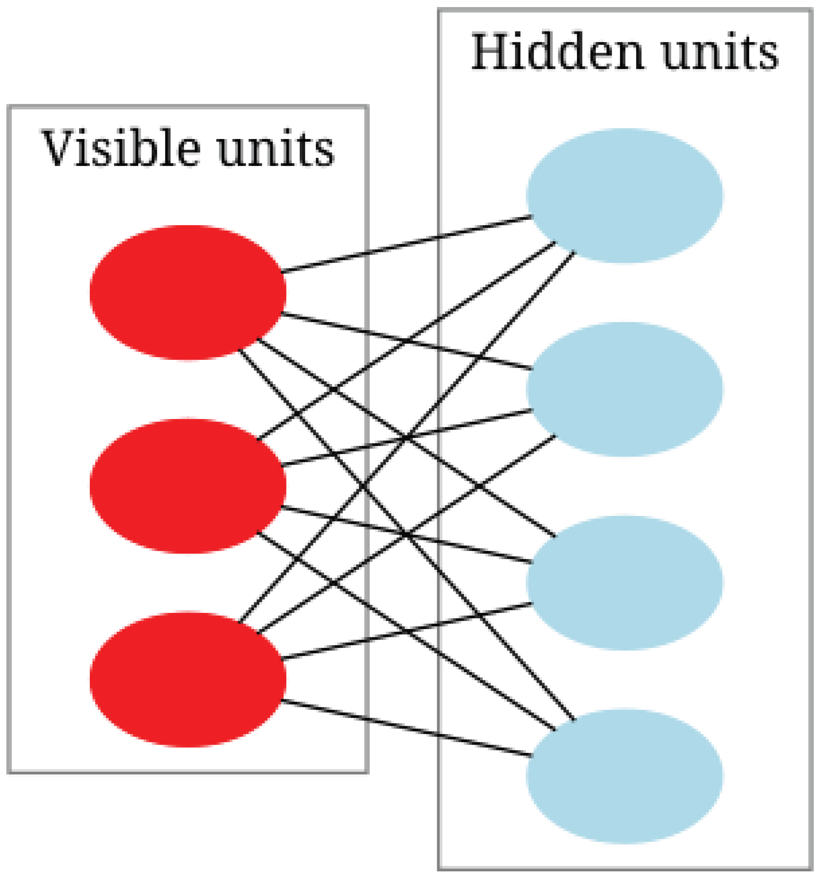 Similarly, the probability of a visible unit given the hidden units is:
The marginal probability of a visible vector is obtained by summing over all possible hidden states:
By factoring out terms dependent only on , we define the free energy function as:
which leads to:
RBMs are trained using gradient descent to minimize the negative log-likelihood:
The gradient of this likelihood function with respect to the weight matrix is given by:
where is the expectation over the training data, is the expectation under the model distribution. The weight updates are then performed using:
RBMs use stochastic gradient descent (SGD) for optimization. The weight updates in SGD follow:
RBMs serve as the building blocks for Deep Belief Networks (DBNs), where multiple RBMs are stacked to form deep architectures. Each layer is pre-trained in an unsupervised manner using contrastive divergence before fine-tuning using backpropagation.
Similarly, the probability of a visible unit given the hidden units is:
The marginal probability of a visible vector is obtained by summing over all possible hidden states:
By factoring out terms dependent only on , we define the free energy function as:
which leads to:
RBMs are trained using gradient descent to minimize the negative log-likelihood:
The gradient of this likelihood function with respect to the weight matrix is given by:
where is the expectation over the training data, is the expectation under the model distribution. The weight updates are then performed using:
RBMs use stochastic gradient descent (SGD) for optimization. The weight updates in SGD follow:
RBMs serve as the building blocks for Deep Belief Networks (DBNs), where multiple RBMs are stacked to form deep architectures. Each layer is pre-trained in an unsupervised manner using contrastive divergence before fine-tuning using backpropagation.
Figure 150.
Diagram of a restricted Boltzmann machine. Image Credit: By Qwertyus - Own work, CC BY-SA 3.0, https://commons.wikimedia.org/w/index.php?curid=22717044. Illustration of a restricted Boltzmann machine featuring three observable units and four concealed units, excluding bias units
Figure 150.
Diagram of a restricted Boltzmann machine. Image Credit: By Qwertyus - Own work, CC BY-SA 3.0, https://commons.wikimedia.org/w/index.php?curid=22717044. Illustration of a restricted Boltzmann machine featuring three observable units and four concealed units, excluding bias units
16.1.6. Deep Belief Networks (DBNs)
16.1.6.1 Literature Review of Deep Belief Networks (DBNs)
Deep Belief Networks (DBNs) have played a transformative role in deep learning by enabling efficient unsupervised pre-training and hierarchical feature extraction. One of the foundational works in this area is by Hinton et al. (2006) [854], who introduced a fast learning algorithm for DBNs that leverages a greedy layer-wise pre-training strategy using Restricted Boltzmann Machines (RBMs). This work addressed the long-standing vanishing gradient problem in deep networks by initializing weights in a way that preserves meaningful feature representations before fine-tuning with supervised learning. Their contribution established DBNs as a key component of early deep learning architectures and laid the groundwork for further explorations into deep generative models. Lee et al. (2009) [1109] extended the standard DBN framework by incorporating convolutional structures, leading to the development of Convolutional Deep Belief Networks (CDBNs). By introducing local receptive fields and weight sharing, CDBNs enabled the automatic discovery of spatial hierarchies in data, making them particularly suitable for image and speech processing applications. This work demonstrated that DBNs could be adapted to structured data representations, enhancing their scalability and generalization capability.
In the domain of speech recognition, Mohamed et al. (2012) [1111] pioneered the application of DBNs for acoustic modeling, demonstrating that these networks could effectively capture complex audio patterns. Their work provided empirical evidence that DBN-based models significantly outperformed traditional Gaussian Mixture Models (GMMs) when used in conjunction with Hidden Markov Models (HMMs) for automatic speech recognition. This breakthrough accelerated the adoption of deep learning in the field of speech processing and motivated subsequent research into deep neural network-based acoustic modeling. Similarly, Zhang and Zhao (2017) [1113] explored the use of DBNs for fault diagnosis in chemical processes, highlighting their ability to model intricate dependencies within multivariate industrial datasets. Their work demonstrated that DBNs could learn compact feature representations from noisy sensor data, leading to improved fault detection accuracy. By applying DBNs to real-world industrial systems, they provided compelling evidence of their practical utility in process monitoring and control.
Further expanding the use of DBNs in fault diagnostics, Peng et al. (2019) [1112] introduced a health indicator construction framework based on DBNs for bearing fault diagnosis. Their approach enabled the automatic extraction of degradation features from vibration signals, allowing for early detection of mechanical failures. The health indicator developed in their study demonstrated superior predictive performance compared to traditional statistical methods, underscoring the power of DBNs in prognostics and health management applications. Zhang et al. (2018) [1115] extended the use of DBNs to the medical field by integrating them with feature selection and extraction methods for predicting clinical outcomes in lung cancer patients. Their study illustrated that DBNs could capture complex interactions between clinical variables, improving the interpretability and accuracy of predictive models in oncology. By leveraging deep learning for medical prognosis, this work demonstrated the potential of DBNs to advance personalized healthcare and decision support systems.
Zhong et. al. (2017) [1118] examined the problem of image classification with limited training data and demonstrated that DBNs could learn meaningful feature representations even in data-scarce settings. Their work emphasized the ability of DBNs to leverage unsupervised pre-training, enabling them to generalize well even when labeled data is insufficient. This contribution reinforced the importance of DBNs in applications where obtaining large-scale labeled datasets is challenging. Financial time series analysis is another domain where DBNs have demonstrated utility. Liu (2018) [1114] proposed a hybrid prediction model that combined DBNs with the Autoregressive Integrated Moving Average (ARIMA) model for stock trend forecasting. Their approach leveraged the pattern recognition capabilities of DBNs along with the time-series forecasting strengths of ARIMA, resulting in improved predictive performance for financial markets. This work showcased the effectiveness of deep learning in modeling complex temporal dependencies and provided insights into how hybrid models could enhance financial decision-making. Jormakka and Ghosh (2021) [1452] introduce a novel method for solving certain stochastic processes using generating functions, derive a general theorem for generating functions of a particular type, and apply this method to obtain polynomial-time algorithms for specific partitions; they further generalize the approach to a broader class of linear transformations and utilize it to develop a theoretical polynomial-time algorithm for the knapsack problem. Ghosh (2021) [1465] provides an accessible exploration of the Arithmetic Mean-Geometric Mean (AM-GM) inequality, offering both elementary and advanced proofs—including an elegant derivation using the exponential function—and demonstrates its applications through classical inequalities such as Nesbitt’s inequality, thereby enhancing understanding of fundamental inequalities in mathematics. Cox and Ghosh (2020) [1479] extend the study of the Collatz conjecture by introducing the concept of generalized dead limbs and analyzing cycles with attachment points, demonstrating that all known cycles for lie within these generalized dead limbs, and suggesting that this containment is a necessary condition for the existence of such cycles. Abhyankar et. al. (2002) [1490] provided a comprehensive overview of the Zeta function, detailing its historical development, key properties, and applications in number theory, and offered an accessible introduction to its significance in modern mathematics. Finally, Hoang and Kang (2018) [1116] developed a novel fault diagnosis framework by integrating DBNs with Dempster–Shafer evidence theory. Their study highlighted how DBNs could serve as a powerful feature extractor while Dempster–Shafer theory facilitated the fusion of information from multiple sources, enhancing fault detection accuracy. This interdisciplinary approach demonstrated the potential of combining deep learning with probabilistic reasoning for more reliable fault diagnosis in engineering systems.
Collectively, these studies illustrate the broad impact of DBNs across multiple domains, including speech recognition, industrial fault diagnosis, medical prognosis, uncertainty quantification, and financial prediction. The ability of DBNs to learn hierarchical representations from high-dimensional data has established them as a powerful tool for tackling complex machine learning problems. The advancements made in adapting DBNs to convolutional architectures, hybrid models, and ensemble methods have further expanded their applicability, ensuring their continued relevance in deep learning research. As interest in deep generative models and representation learning grows, DBNs continue to serve as a foundational framework for understanding and developing more sophisticated deep learning architectures.
Table 14.
Summary of Contributions on Deep Belief Networks (DBNs)
| Authors (Year) | Contribution |
|---|---|
| Hinton et al. (2006) [854] | Introduced a fast learning algorithm for DBNs using a greedy layer-wise pre-training strategy based on Restricted Boltzmann Machines (RBMs). Addressed the vanishing gradient problem and established DBNs as foundational deep learning architectures. |
| Lee et al. (2009) [1109] | Developed Convolutional Deep Belief Networks (CDBNs) by incorporating convolutional structures into DBNs, introducing local receptive fields and weight sharing for improved scalability in image and speech processing. |
| Mohamed et al. (2012) [1111] | Pioneered the application of DBNs for acoustic modeling in speech recognition, demonstrating superior performance over traditional Gaussian Mixture Models (GMMs) in conjunction with Hidden Markov Models (HMMs). |
| Zhang and Zhao (2017) [1113] | Applied DBNs for fault diagnosis in chemical processes, showing that DBNs effectively model dependencies in multivariate datasets and enhance fault detection accuracy. |
| Peng et al. (2019) [1112] | Developed a DBN-based health indicator construction framework for bearing fault diagnosis, enabling automatic extraction of degradation features from vibration signals for early failure detection. |
| Zhang et al. (2018) [1115] | Integrated DBNs with feature selection methods for predicting clinical outcomes in lung cancer patients, enhancing predictive accuracy and interpretability in medical prognosis. |
| Zhong et. al. (2017) [1118] | Demonstrated that DBNs could learn meaningful representations even with limited training data, reinforcing their utility in scenarios with scarce labeled datasets. |
| Liu (2018) [1114] | Combined DBNs with the Autoregressive Integrated Moving Average (ARIMA) model for stock trend forecasting, leveraging DBNs’ pattern recognition capabilities with ARIMA’s time-series forecasting strengths. |
| Hoang and Kang (2018) [1116] | Developed a novel fault diagnosis framework by integrating DBNs with Dempster–Shafer evidence theory, enhancing fault detection accuracy through probabilistic reasoning. |
16.1.6.2 Recent Literature Review of Deep Belief Networks (DBNs)
Deep Belief Networks (DBNs) have emerged as a powerful deep learning architecture capable of hierarchical feature learning and unsupervised pre-training. These networks, based on a stack of Restricted Boltzmann Machines (RBMs), have been widely used in various fields, ranging from human activity recognition and medical diagnosis to cybersecurity and agricultural applications. Joudaki (2025) [1100] provides an extensive literature review on the theoretical underpinnings of DBNs and RBMs, emphasizing their role in human action recognition. The study highlights how DBNs are particularly suited for tasks requiring high-dimensional feature extraction and learning temporal dependencies, outperforming traditional machine learning models. The hierarchical representation learned by DBNs allows them to capture complex patterns in human gestures and postures, making them ideal for applications such as motion tracking and gesture-based interface design.
Alzughaibi (2025) [1119] presents an innovative application of DBNs in pest detection, where they are integrated with a modified artificial hummingbird algorithm. The research demonstrates how deep learning-based pattern recognition models can significantly enhance the accuracy of pest classification in agricultural settings. The model is trained on large datasets of pest images, leveraging the hierarchical feature extraction capabilities of DBNs to distinguish between different species effectively. Similarly, Savitha et al. (2025) [1103] apply DBNs to cardiovascular disease prediction by integrating them with the Harris Hawks Search optimization algorithm. This approach optimizes feature selection and classification accuracy, showing that DBNs can be successfully adapted for medical diagnosis by leveraging their deep hierarchical structure. The study underscores the potential of DBNs in clinical decision support systems, where accurate and timely diagnoses are crucial.
The intrinsic hierarchical structure of DBNs has also been studied by Tausani et al. (2025) [1120], who investigate their top-down inference capabilities compared to other deep generative models. Their research explores how DBNs can simulate human-like cognition and learning, making them suitable for applications in artificial intelligence and cognitive computing. By analyzing the internal feature representations of DBNs, the study provides insights into their interpretability and efficiency in generative tasks. Kumar and Ravi (2025) [1121] further contribute to the field by introducing XDATE, an explainable deep learning framework that combines DBNs with auto-encoders. The study addresses the issue of interpretability in deep learning by employing the Garson Algorithm to improve feature attribution, demonstrating that DBNs can achieve a balance between accuracy and explainability in classification tasks.
In the field of medical image analysis, Alhajlah (2024) [1122] applies DBNs for automated lesion detection in gastrointestinal endoscopic images. The research integrates DBNs with a genetic algorithm-based segmentation technique, significantly improving diagnostic precision. By leveraging the feature extraction capabilities of DBNs, the proposed system outperforms conventional image processing techniques, reducing false positives and improving lesion classification accuracy. Hossain et al. (2025) [1107] evaluate the performance of DBNs in human activity recognition, benchmarking them against various classical and deep learning models. Their study finds that DBNs, despite being unsupervised in their initial training phase, can achieve competitive accuracy on small and medium-sized datasets, demonstrating their robustness and adaptability.
The application of DBNs extends to cybersecurity, where Pavithra et al. (2025) [1123] develop a hybrid RNN-DBN model for detecting IoT attacks. This approach captures temporal dependencies in network traffic, allowing for effective anomaly detection and threat mitigation. The fusion of DBNs with recurrent networks enables better sequence modeling, making them highly effective in cybersecurity applications. In a similar vein, Bhadane and Verma (2024) [1124] explore the role of DBNs in personality trait classification, comparing their performance with CNNs and RNNs. Their study highlights the advantages of DBNs in handling high-dimensional psychological datasets, where deep hierarchical structures enable the capture of complex personality-related patterns. Lastly, Keivanimehr and Akbari (2025) [1125] examine how DBNs can be applied in edge computing for cardiovascular disease monitoring. Their research discusses the feasibility of deploying DBN-based models in TinyML environments, where computational efficiency and real-time processing are critical.
Collectively, these studies demonstrate the versatility and efficacy of DBNs in various domains, from healthcare and cybersecurity to agricultural automation and cognitive computing. The hierarchical feature learning capabilities of DBNs, combined with their ability to leverage unsupervised pre-training, make them suitable for a wide range of complex tasks. Future research is likely to explore further hybrid architectures that integrate DBNs with more advanced deep learning models, enhancing their adaptability and efficiency in real-world applications.
Table 15.
Summary of Contributions
| Authors (Year) | Contribution |
|---|---|
| Joudaki (2025) [1100] | Provides an extensive literature review on the theoretical foundations of DBNs and RBMs, emphasizing their role in human action recognition. Demonstrates their effectiveness in capturing complex patterns in human gestures and postures for applications such as motion tracking and gesture-based interface design. |
| Alzughaibi (2025) [1119] | Applies DBNs in pest detection, integrating them with a modified artificial hummingbird algorithm. Enhances pest classification accuracy using deep hierarchical feature extraction on large image datasets. |
| Savitha et al. (2025) [1103] | Employs DBNs for cardiovascular disease prediction, integrating them with the Harris Hawks Search optimization algorithm. Demonstrates improved feature selection and classification accuracy in medical diagnosis applications. |
| Tausani et al. (2025) [1120] | Investigates the top-down inference capabilities of DBNs compared to other deep generative models. Explores their interpretability and efficiency in artificial intelligence and cognitive computing tasks. |
| Kumar and Ravi (2025) [1121] | Introduces XDATE, an explainable deep learning framework that combines DBNs with auto-encoders. Uses the Garson Algorithm to enhance feature attribution, balancing accuracy and interpretability in classification tasks. |
| Alhajlah (2024) [1122] | Applies DBNs in medical image analysis for automated lesion detection in gastrointestinal endoscopic images. Integrates DBNs with a genetic algorithm-based segmentation technique to enhance diagnostic precision and reduce false positives. |
| Hossain et al. (2025) [1107] | Benchmarks DBNs against classical and deep learning models for human activity recognition. Demonstrates DBNs’ robustness and adaptability, particularly in small and medium-sized datasets. |
| Pavithra et al. (2025) [1123] | Develops a hybrid RNN-DBN model for IoT attack detection, capturing temporal dependencies in network traffic for anomaly detection and threat mitigation. |
| Bhadane and Verma (2024) [1124] | Explores DBNs for personality trait classification, comparing their performance with CNNs and RNNs. Highlights the advantages of DBNs in processing high-dimensional psychological datasets. |
| Keivanimehr and Akbari (2025) [1125] | Investigates DBNs for edge computing applications in cardiovascular disease monitoring. Discusses feasibility in TinyML environments for computational efficiency and real-time processing. |
16.1.6.3 Mathematical Analysis of Deep Belief Networks (DBNs)
A Deep Belief Network (DBN) is a generative graphical model composed of multiple layers of stochastic latent variables, typically represented as Restricted Boltzmann Machines (RBMs) stacked hierarchically. The fundamental structure of a DBN is built upon the principles of probabilistic modeling, unsupervised pretraining, and layer-wise greedy learning to form a deep hierarchical representation of data. Mathematically, a DBN is a composition of multiple RBMs, each trained independently in a bottom-up fashion, followed by fine-tuning using backpropagation when supervised learning is required. The probabilistic nature of DBNs allows them to model complex joint probability distributions over observed and latent variables, making them highly effective for feature extraction, dimensionality reduction, and generative modeling.
Let denote the input data vector, where d is the dimensionality of the input space. A DBN consists of multiple layers of hidden variables connected in a directed fashion in the upper layers and undirected in the lower layers. The network defines a joint probability distribution over the visible units and hidden units as follows:
where:
- represents the conditional distribution of the visible layer given the first hidden layer.
- represents the conditional dependency between consecutive layers.
- represents the top-layer prior, which is modeled as a Restricted Boltzmann Machine (RBM).
Figure 151.
Diagram of a Deep belief network. Image Credit: By Qwertyus - Own work, CC0, https://commons.wikimedia.org/w/index.php?curid=30324766. Diagrammatic representation of a deep belief network, where the arrows indicate directed connections within the corresponding graphical model
Figure 151.
Diagram of a Deep belief network. Image Credit: By Qwertyus - Own work, CC0, https://commons.wikimedia.org/w/index.php?curid=30324766. Diagrammatic representation of a deep belief network, where the arrows indicate directed connections within the corresponding graphical model
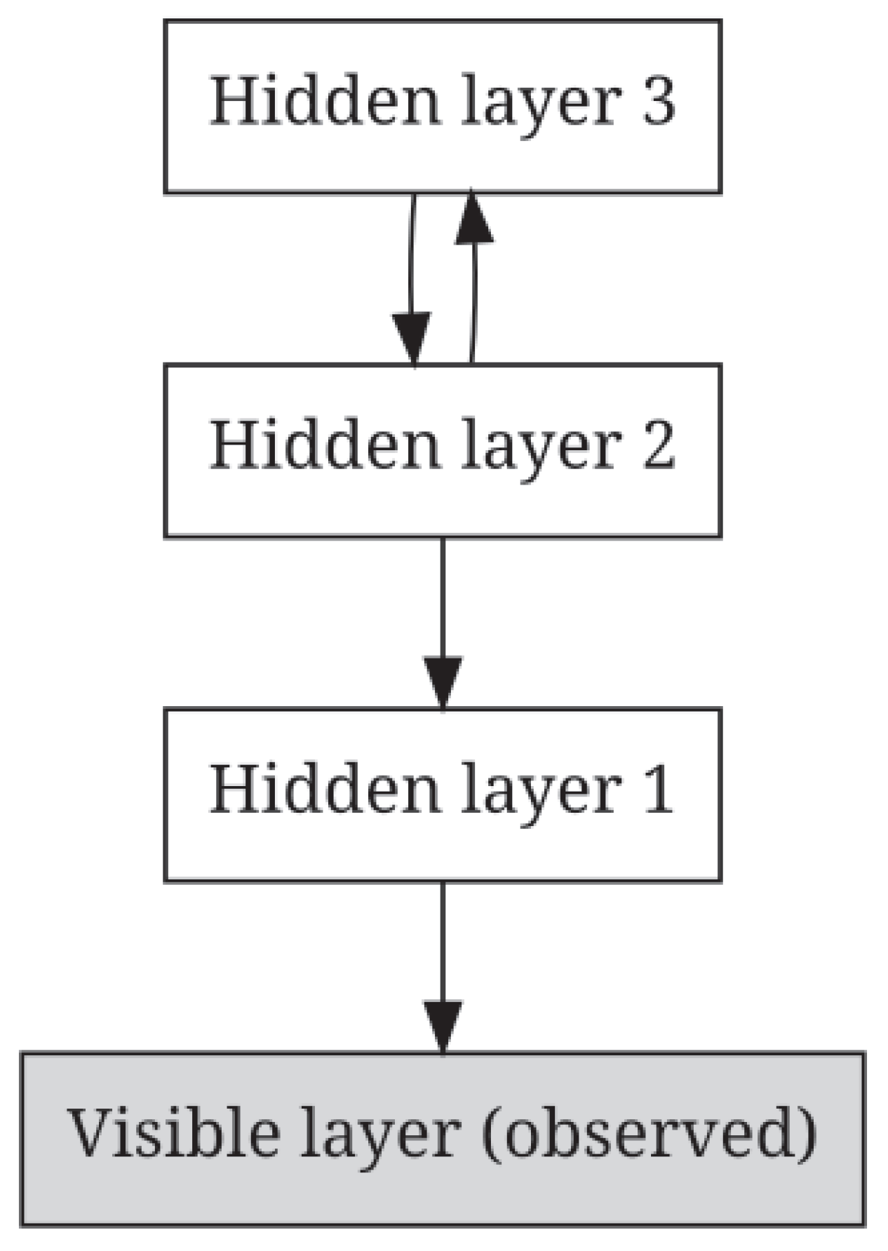
Restricted Boltzmann Machine (RBM) as a Building Block
Each RBM consists of a layer of visible units and a layer of hidden units , with energy function given by:
where are the binary visible units, are the binary hidden units, is the weight matrix connecting visible and hidden units, and are the bias terms for visible and hidden units, respectively. The probability distribution over is given by the Boltzmann distribution:
where Z is the partition function:
Since exact inference in RBMs is intractable due to the exponential summation in Z, we use Contrastive Divergence (CD) to approximate the gradient:
Layer-wise Pretraining of DBNs
DBNs are trained using a layer-wise greedy learning algorithm, which first trains each RBM independently and then stacks them hierarchically. Given an input dataset , the pretraining procedure follows:
- Train the first RBM with input to obtain hidden activations:
- Use hidden activations as input for training the second RBM:
Fine-Tuning with Backpropagation
Once pretraining is complete, DBNs can be fine-tuned using backpropagation if labeled data is available. A cost function such as cross-entropy loss is used:
The gradients are computed using:
Deep Belief Networks (DBNs) serve as powerful generative models capable of capturing hierarchical representations of data through layer-wise pretraining of RBMs.
16.1.7. t-Distributed Stochastic Neighbor Embedding (t-SNE)
16.1.7.1 Literature Review of t-Distributed Stochastic Neighbor Embedding
T-distributed Stochastic Neighbor Embedding (t-SNE) has been widely studied and refined since its introduction, with various works expanding its theoretical foundations, applications, and practical optimizations. The foundational work of van der Maaten and Hinton (2008) [1042] introduced t-SNE as an improvement over Stochastic Neighbor Embedding (SNE), primarily by incorporating a symmetric probability distribution in the low-dimensional space and replacing the Gaussian-based similarity measure with a heavy-tailed Student’s t-distribution to address the crowding problem. This innovation enabled better preservation of both local and global structures when mapping high-dimensional data into lower dimensions. The study established the mathematical formulation of t-SNE by minimizing the Kullback-Leibler divergence between joint probability distributions of data points in high and low dimensions, leading to a widely adopted visualization tool in machine learning and data science.
Several studies have analyzed and improved the robustness of t-SNE, particularly concerning its application to large datasets and biological data visualization. Kobak and Berens (2019) [1126] addressed the challenges in single-cell transcriptomics by developing "opt-SNE," an automated parameter selection framework that fine-tunes the perplexity and learning rate to enhance visualization reliability. Their study demonstrated that proper parameter tuning significantly impacts the quality of embeddings, thereby reducing the risk of misleading interpretations. Similarly, Belkina et al. (2019) [1127] proposed an automated approach for optimizing t-SNE parameters for large datasets, emphasizing the importance of reproducibility and interpretability in real-world applications. Their work provided empirical evidence that parameter selection can drastically affect the clustering structure in t-SNE visualizations, necessitating automated approaches for better standardization.
Beyond empirical studies, some researchers have sought to establish a more rigorous theoretical understanding of t-SNE’s behavior in clustering and manifold learning. Linderman and Steinerberger (2019) [1128] provided a mathematical proof that t-SNE effectively recovers well-separated clusters under certain conditions, offering a theoretical foundation for why t-SNE performs well in clustering applications despite not being explicitly designed for that purpose. Their work bridged the gap between empirical success and mathematical justification, thereby enhancing the credibility of t-SNE in scientific applications. Amorim and Mirkin (2012) [1129] extended this discussion by exploring the role of distance metrics in clustering and feature weighting, providing an alternative approach that incorporated Minkowski metrics and anomaly detection within the t-SNE-reduced space. Their work showed that selecting an appropriate distance function could further refine the clustering properties of dimensionality reduction methods, leading to improved segmentation of data points. Additionally, Wattenberg et al. (2016) [1130] provided a detailed discussion on how to use t-SNE effectively, emphasizing the interpretational pitfalls and practical considerations when applying t-SNE to real-world data. Their work highlighted the limitations of t-SNE in preserving global structure and warned against misinterpreting distance relationships in the lower-dimensional space.
In response to computational challenges, Pezzotti et al. (2016) [1131] proposed an approximation method that enabled real-time, user-steerable t-SNE for progressive visual analytics. Their work significantly reduced the computational burden of t-SNE by introducing an interactive framework that allowed users to refine embeddings dynamically, making t-SNE more practical for large-scale applications. Similarly, Kobak and Linderman (2021) [1132] investigated the importance of initialization strategies for preserving global data structures in both t-SNE and UMAP embeddings. Their findings demonstrated that different initialization schemes can lead to drastically different embeddings, underscoring the need for careful selection of initialization methods to ensure meaningful visualizations.
Finally, alternative approaches to t-SNE have been explored, with studies comparing its performance against other dimensionality reduction techniques. Becht et al. (2019) [1133] introduced Uniform Manifold Approximation and Projection (UMAP) as an alternative to t-SNE, arguing that UMAP offers improved scalability and better preservation of global structures. Their study provided empirical comparisons between UMAP and t-SNE, demonstrating that UMAP performs comparably in clustering while requiring significantly less computational time. Likewise, Moon et al. (2019) [1134] proposed PHATE (Potential of Heat-diffusion for Affinity-based Transition Embedding), which was designed to capture both local and global structures more effectively than t-SNE. Their study showcased PHATE’s ability to preserve continuous trajectories in biological data, highlighting its advantages in studying cell differentiation processes. Collectively, these studies illustrate the ongoing efforts to refine and expand upon t-SNE, both theoretically and practically, ensuring its continued relevance in high-dimensional data visualization.
Table 16.
Summary of Contributions in t-SNE Literature Review
| Authors (Year) | Contribution |
|---|---|
| van der Maaten and Hinton (2008) [1042] | Introduced t-SNE as an extension of Stochastic Neighbor Embedding (SNE) by incorporating a Student’s t-distribution to address the crowding problem. This modification improved the preservation of both local and global structures and formulated t-SNE as an optimization problem minimizing Kullback-Leibler divergence. |
| Kobak and Berens (2019) [1126] | Developed "opt-SNE," an automated parameter selection framework for fine-tuning perplexity and learning rate in t-SNE. Their work demonstrated that proper parameter selection significantly affects embedding quality and reduces misleading visualizations in single-cell transcriptomics. |
| Belkina et al. (2019) [1127] | Proposed an optimized pipeline for selecting t-SNE parameters, focusing on reproducibility and interpretability in large-scale biological datasets. Their work emphasized the importance of standardizing parameter selection to improve clustering outcomes in t-SNE applications. |
| Linderman and Steinerberger (2019) [1128] | Provided a mathematical proof that t-SNE reliably recovers well-separated clusters under specific conditions, bridging the gap between empirical observations and theoretical guarantees in clustering applications. |
| Amorim and Mirkin (2012) [1129] | Investigated the role of distance metrics in t-SNE clustering, proposing the use of Minkowski metrics and feature weighting to refine cluster separation. Their work highlighted how different distance functions influence embedding outcomes. |
| Wattenberg et al. (2016) [1130] | Analyzed interpretational pitfalls in t-SNE, cautioning against misinterpretation of distances in low-dimensional embeddings. Their study outlined best practices for applying t-SNE in real-world data visualization tasks. |
| Pezzotti et al. (2016) [1131] | Developed a real-time, user-steerable t-SNE method that enabled progressive visual analytics. Their approach reduced computational overhead and allowed for interactive exploration of embeddings in large-scale applications. |
| Kobak and Linderman (2021) [1132] | Investigated initialization strategies for t-SNE and UMAP, demonstrating that different initialization schemes lead to vastly different embeddings. Their study emphasized the importance of careful initialization to preserve global data structures. |
| Becht et al. (2019) [1133] | Introduced UMAP as an alternative to t-SNE, showing that UMAP provides improved scalability and better preservation of global structures while requiring significantly less computational time. |
| Moon et al. (2019) [1134] | Proposed PHATE as a dimensionality reduction technique designed to capture both local and global structures more effectively than t-SNE. Their study demonstrated PHATE’s superiority in visualizing continuous biological trajectories, such as cell differentiation processes. |
16.1.7.2 Recent Literature Review of t-Distributed Stochastic Neighbor Embedding
t-Distributed Stochastic Neighbor Embedding (t-SNE) has emerged as a powerful tool in high-dimensional data visualization, finding extensive applications across various domains, including biomedical sciences, material science, deep learning, and geophysics. Rivera and Deniega (2025) [1135] demonstrated the efficacy of t-SNE in automating flow cytometry gating, where the method was combined with clustering techniques such as DBSCAN and PCA. Their study highlighted how t-SNE facilitates better separation and classification of cell populations, ultimately improving computational efficiency in biomedical applications. Similarly, Chang (2025) [1136] provided a rigorous survey of dimensionality reduction techniques, discussing the advantages and limitations of t-SNE compared to traditional methods like PCA and newer alternatives like UMAP. The study outlined the scenarios where t-SNE performs optimally, particularly in non-linear data distributions, making it an essential reference for researchers selecting appropriate dimensionality reduction techniques.
In the domain of defect detection in industrial settings, Chern et al. (2025) [1137] utilized t-SNE for visualizing metal defect classification in deep learning models, improving interpretability in YOLO-based defect detection frameworks. Their study showed how t-SNE enhances the understanding of feature similarities among defect classes, leading to more refined model improvements. A similar approach was adopted by Li et al. (2025) [1138] in the field of food safety, where t-SNE was applied to olfactory sensor data to analyze aflatoxin B1 contamination in wheat. By employing t-SNE for dimensionality reduction, the researchers effectively visualized sensor response variations, demonstrating the method’s utility in complex chemical data analysis. In another domain, Singh and Singh (2025) [1139] developed a hybrid approach for medical image retrieval by integrating deep learning features with t-SNE. Their method showed that t-SNE enhances feature clustering, thereby improving the accuracy and efficiency of gastric image retrieval systems, which is particularly beneficial in computer-aided diagnosis applications.
Sun et al. (2025) [1142] explored the application of t-SNE in biomechanics, specifically in detecting muscle fatigue during lower limb isometric contraction tasks. Their study employed t-SNE to reduce the dimensionality of electromyography (EMG) data before applying machine learning-based classification, leading to improved performance in fatigue detection models. Meanwhile, Su et al. (2025) [1143] incorporated t-SNE into seismic fragility analysis for earth-rock dams, integrating it within a deep residual shrinkage network to enhance predictive accuracy. Their research illustrated how t-SNE, when combined with deep learning techniques, can refine the interpretation of heterogeneous material behavior under seismic loading conditions. In the biomedical domain, Yousif and Al-Sarray (2025) [1144] integrated t-SNE with spectral clustering via convex optimization to enhance breast cancer gene classification. Their work established that this combination yields superior clustering performance compared to conventional methods, contributing significantly to genomics research and precision medicine.
Park et al. (2025) [1145] assessed the clinical applicability of t-SNE in flow cytometry, specifically for hematologic malignancies. Their study compared t-SNE with UMAP in reducing high-dimensional cytometric data and concluded that t-SNE provides superior local structure preservation, which is crucial for identifying rare cell populations in clinical diagnostics. Qiao et al. (2025) [1146] used t-SNE to analyze cancer-associated fibroblasts (CAFs) in pancreatic ductal adenocarcinoma patients, identifying subclusters that exhibited distinct inflammatory gene expression patterns. This study underscored the value of t-SNE in uncovering hidden patterns in complex biological datasets, aiding in the stratification of cancer patients based on gene expression profiles. Furthermore, t-SNE has been utilized in aerospace engineering, as demonstrated by Su et al. (2025) [1143], who employed the technique in damage quantification for aircraft structures. Their study integrated t-SNE into an end-to-end deep learning framework to enhance defect localization, demonstrating how the method can improve structural health monitoring systems.
Overall, these studies collectively emphasize the versatility of t-SNE across diverse fields, ranging from biomedical sciences and geophysics to industrial defect detection and aerospace engineering. While t-SNE’s strength lies in its ability to preserve local structures in high-dimensional data, these studies also highlight its limitations, such as high computational cost and sensitivity to parameter tuning. Future research should focus on optimizing t-SNE’s efficiency while maintaining its robust visualization capabilities. By integrating t-SNE with deep learning architectures and hybrid clustering techniques, researchers can further expand its applications in fields requiring advanced data analysis and interpretation. The increasing adoption of t-SNE across disciplines highlights its ongoing relevance, making it a crucial tool for researchers handling complex, high-dimensional datasets.
Table 17.
Summary of Recent Contributions in t-SNE Literature Review
| Authors (Year) | Contribution |
|---|---|
| Rivera and Deniega (2025) [1135] | Demonstrated the efficacy of t-SNE in automating flow cytometry gating, improving cell population classification using clustering techniques such as DBSCAN and PCA. |
| Chang (2025) [1136] | Provided a survey of dimensionality reduction techniques, analyzing the strengths and weaknesses of t-SNE compared to PCA and UMAP, emphasizing its performance on non-linear data distributions. |
| Chern et al. (2025) [1137] | Applied t-SNE for visualizing metal defect classification in YOLO-based deep learning models, enhancing interpretability in industrial defect detection. |
| Li et al. (2025) [1138] | Utilized t-SNE for olfactory sensor data analysis in detecting aflatoxin B1 contamination in wheat, demonstrating its utility in chemical data visualization. |
| Singh and Singh (2025) [1139] | Developed a hybrid medical image retrieval approach by integrating deep learning features with t-SNE, improving clustering and accuracy in gastric image retrieval systems. |
| Sun et al. (2025) [1142] | Investigated t-SNE’s application in biomechanics, reducing the dimensionality of electromyography (EMG) data for improved muscle fatigue classification. |
| Su et al. (2025) [1143] | Incorporated t-SNE in seismic fragility analysis of earth-rock dams, enhancing predictive accuracy when integrated into a deep residual shrinkage network. |
| Yousif and Al-Sarray (2025) [1144] | Combined t-SNE with spectral clustering via convex optimization for breast cancer gene classification, achieving superior clustering performance over conventional methods. |
| Park et al. (2025) [1145] | Assessed the use of t-SNE in flow cytometry for hematologic malignancies, highlighting its superiority in preserving local structures compared to UMAP. |
| Qiao et al. (2025) [1146] | Applied t-SNE to analyze cancer-associated fibroblasts (CAFs) in pancreatic ductal adenocarcinoma, identifying gene expression subclusters for patient stratification. |
| Su et al. (2025) [1143] | Employed t-SNE for damage quantification in aircraft structures, integrating it into a deep learning framework to enhance structural health monitoring. |
16.1.7.3 Mathematical Analysis of t-Distributed Stochastic Neighbor Embedding
The t-distributed stochastic neighbor embedding (t-SNE) algorithm, developed by Laurens van der Maaten and Geoffrey Hinton, is a nonlinear dimensionality reduction technique particularly well-suited for visualizing high-dimensional datasets in lower dimensions (typically 2D or 3D). At its core, t-SNE aims to preserve the local structure of data points by modeling pairwise similarities in both high-dimensional and low-dimensional spaces and minimizing the discrepancy between these similarities. The method builds upon Stochastic Neighbor Embedding (SNE) by incorporating a Student’s t-distribution with a single degree of freedom (i.e., a Cauchy distribution) as the low-dimensional similarity function, significantly mitigating the crowding problem of SNE. The mathematical formulation of t-SNE is highly intricate and involves defining probability distributions over pairwise relationships, constructing a cost function based on Kullback-Leibler (KL) divergence, and employing gradient-based optimization methods such as gradient descent to find an embedding that best preserves local structures.
Constructing the High-Dimensional Probability Distribution
Let be a set of N data points in a high-dimensional space of dimension D. We define a conditional probability distribution that represents the similarity between points and based on a Gaussian distribution centered at . The probability that is a neighbor of is given by:
where is the perplexity-dependent bandwidth parameter for point , which controls how much influence distant points have on similarity measures.
Figure 152.
T-SNE representation of word embeddings derived from 19th-century literary texts. Image Credit: By Siobhán Grayson, CC BY-SA 4.0, https://commons.wikimedia.org/w/index.php?curid=64541584
Figure 152.
T-SNE representation of word embeddings derived from 19th-century literary texts. Image Credit: By Siobhán Grayson, CC BY-SA 4.0, https://commons.wikimedia.org/w/index.php?curid=64541584
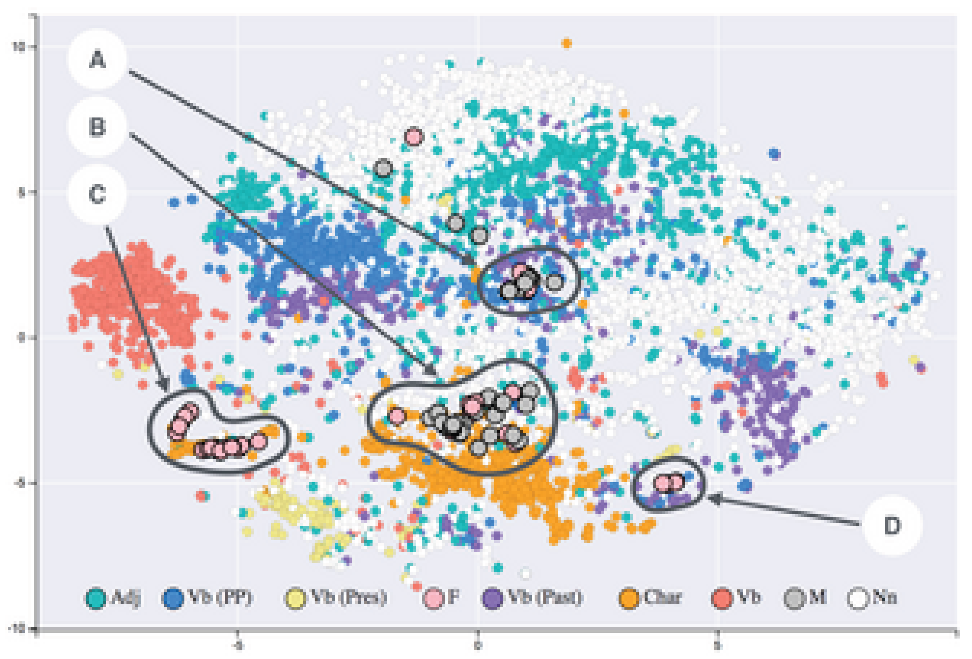
Figure 153.
T-SNE embeddings of MNIST dataset. Image Credit: By Kyle McDonald - https://www.flickr.com/photos/kylemcdonald/26620503329/, CC BY 2.0, https://commons.wikimedia.org/w/index.php?curid=115726949
Figure 153.
T-SNE embeddings of MNIST dataset. Image Credit: By Kyle McDonald - https://www.flickr.com/photos/kylemcdonald/26620503329/, CC BY 2.0, https://commons.wikimedia.org/w/index.php?curid=115726949
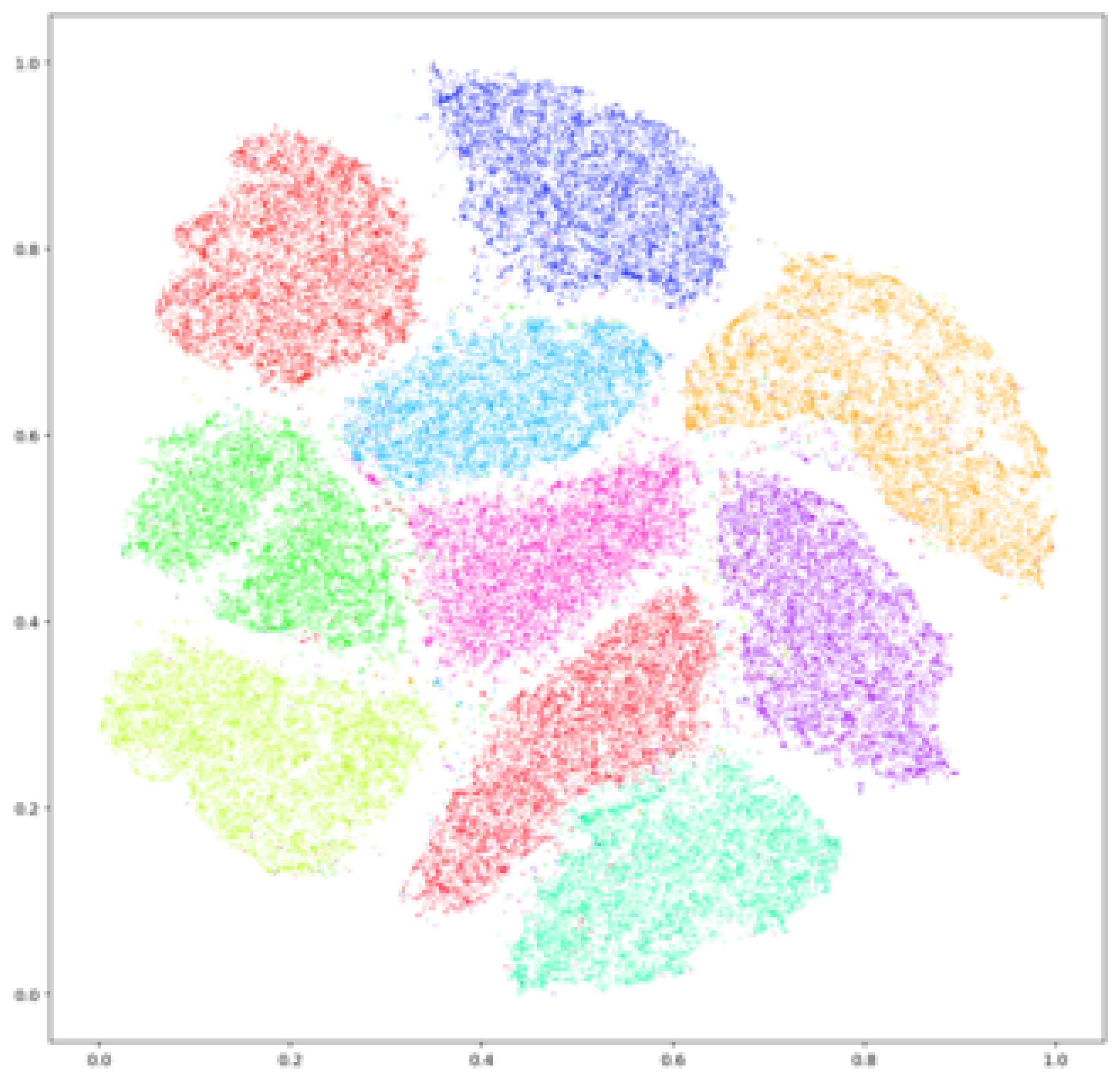
The perplexity, denoted as , is defined as:
where is the Shannon entropy of the probability distribution:
We then symmetrize these conditional probabilities to obtain a symmetric joint probability distribution:
This ensures that , making optimization easier and avoiding directed relationships between points.
Constructing the Low-Dimensional Probability Distribution
We now define a probability distribution in the lower-dimensional space (typically 2D or 3D) with corresponding mapped points (where ). Instead of a Gaussian kernel, t-SNE employs a Student’s t-distribution with one degree of freedom (a Cauchy distribution) to measure similarities:
This choice of the t-distribution helps mitigate the crowding problem, where points in high-dimensional space that are moderately distant tend to collapse together in low-dimensional space when using Gaussian similarities.
The Kullback-Leibler Divergence Cost Function
To ensure that the probability distributions and match as closely as possible, we minimize the Kullback-Leibler (KL) divergence, which measures how much information is lost when using to approximate :
This function is minimized using gradient descent, where the gradient with respect to each low-dimensional point is given by:
Optimization Using Momentum-Based Gradient Descent
To find an optimal configuration of points in the lower-dimensional space, we iteratively update using an adaptive learning rate and a momentum term to prevent getting stuck in local minima:
where is the learning rate, is the momentum coefficient, and represents positions at different iterations.
In summary, t-SNE is a powerful, highly nonlinear technique for dimensionality reduction that excels at visualizing high-dimensional data while preserving local structures. Its formulation relies on constructing two probability distributions, using a t-distribution kernel, and optimizing the KL divergence cost function through gradient descent. However, due to its computational complexity, improvements such as Barnes-Hut t-SNE and FIt-SNE have been developed for large datasets.
16.1.8. Locally Linear Embedding (LLE)
16.1.8.1 Literature Review of Locally Linear Embedding (LLE)
Locally Linear Embedding (LLE), introduced by Roweis and Saul (2000) [1043], is a nonlinear dimensionality reduction method that aims to preserve the local geometric properties of high-dimensional data while embedding it into a lower-dimensional space. The core idea behind LLE is to represent each data point as a linear combination of its nearest neighbors and then determine the low-dimensional representation that best preserves these local linear reconstructions. Unlike methods such as Principal Component Analysis (PCA) or Multidimensional Scaling (MDS), LLE does not assume a global linear structure but instead relies on local affine invariances to extract meaningful low-dimensional embeddings. Saul and Roweis (2000) [1147] later provided an in-depth mathematical exposition of the LLE algorithm, detailing its optimization formulation and demonstrating its capability to uncover nonlinear manifold structures. Their work emphasized that LLE effectively preserves local symmetries without requiring an explicit parametrization of the data manifold, thus making it suitable for a wide range of applications in machine learning and data analysis.
Following the introduction of LLE, Polito and Perona (2001) [1148] extended its application to the problem of clustering and dimensionality reduction, demonstrating that LLE could naturally group data points based on their intrinsic geometric properties. Their study highlighted the algorithm’s ability to perform soft clustering, where different regions of the embedded space correspond to distinct clusters in the high-dimensional space. This property is particularly useful in vision tasks where the underlying data often exhibit complex nonlinear structures. Zhang and Zha (2004) [1150] proposed an alternative approach to nonlinear dimensionality reduction known as Local Tangent Space Alignment (LTSA), which sought to align local tangent spaces rather than simply preserving locally linear relationships. By focusing on the consistency of local tangent approximations, LTSA addressed certain limitations of LLE, particularly its sensitivity to variations in neighborhood density. LTSA improved the quality of embeddings by ensuring a more faithful reconstruction of the global manifold structure, thereby making it a competitive alternative to LLE for high-dimensional data analysis.
Further refinements to LLE were made by Donoho and Grimes (2003) [1151], who introduced Hessian Eigenmaps as a variation of LLE that utilized Hessian-based quadratic forms to better capture local curvature information. Their work showed that Hessian Eigenmaps could outperform standard LLE in cases where the data exhibited significant variations in local density, thereby reducing distortion in the learned embeddings. Another modification, introduced by Zhang and Wang (2006) [1152], was the development of Modified Locally Linear Embedding (MLLE), which incorporated multiple weights in each neighborhood to address issues related to the conditioning of the local weight matrix. The authors demonstrated that by introducing multiple weight constraints, MLLE produced embeddings that were less prone to numerical instability, thus leading to improved robustness and consistency in the low-dimensional representations. These advancements collectively enhanced the stability and general applicability of LLE-based methods, reinforcing their utility in real-world machine learning tasks.
Beyond theoretical refinements, LLE found applications in natural language processing, where Liang (2005) [1153] explored its role in semi-supervised learning. By leveraging the geometric structure of unlabeled data, LLE facilitated the discovery of meaningful feature representations, which proved useful in learning linguistic patterns with limited labeled samples. Coates and Ng (2012) [1154] provided a broader perspective on feature learning by comparing LLE with other unsupervised learning techniques such as K-means clustering. Their study examined the strengths and weaknesses of LLE in the context of automatic feature extraction, highlighting its capacity to learn meaningful data representations without explicit supervision. These contributions underscored the versatility of LLE and its relevance across different domains, including computer vision, speech processing, and text analysis.
In the broader context of feature extraction and representation learning, Hyvärinen and Oja (2000) [1155] explored Independent Component Analysis (ICA) as an alternative method for learning structured representations of high-dimensional data. While ICA seeks to identify statistically independent components, LLE preserves local geometric relationships, making them complementary approaches to dimensionality reduction. Lee et al. (2006) [1156] further advanced the study of feature learning by developing efficient sparse coding algorithms, which provided insights into the underlying structures of data representations. Their work discussed the differences between sparse coding techniques and manifold learning approaches such as LLE, emphasizing the advantages of sparsity constraints in generating interpretable features. Collectively, these contributions illustrate the ongoing evolution of nonlinear dimensionality reduction techniques, with LLE serving as a foundational method that continues to inspire research in machine learning and data science.
Table 18.
Summary of Contributions in Locally Linear Embedding (LLE)
| Authors (Year) | Contribution |
| Roweis and Saul (2000) [1043] | Introduced Locally Linear Embedding (LLE), a nonlinear dimensionality reduction method that preserves local geometric properties while embedding high-dimensional data into a lower-dimensional space. LLE represents each data point as a linear combination of its nearest neighbors and determines an embedding that best preserves these local reconstructions. |
| Saul and Roweis (2000) [1147] | Provided an in-depth mathematical exposition of the LLE algorithm, detailing its optimization formulation and demonstrating its effectiveness in uncovering nonlinear manifold structures without requiring explicit parametrization of the data manifold. |
| Polito and Perona (2001) [1148] | Extended LLE to clustering and dimensionality reduction, showing that LLE naturally groups data points based on intrinsic geometric properties, allowing for soft clustering useful in vision tasks. |
| Zhang and Zha (2004) [1150] | Proposed Local Tangent Space Alignment (LTSA), which aligns local tangent spaces rather than preserving local linear relationships, addressing LLE’s sensitivity to variations in neighborhood density and improving global manifold reconstruction. |
| Donoho and Grimes (2003) [1151] | Introduced Hessian Eigenmaps, a variation of LLE utilizing Hessian-based quadratic forms to capture local curvature, reducing distortion in embeddings for data with significant variations in local density. |
| Zhang and Wang (2006) [1152] | Developed Modified Locally Linear Embedding (MLLE), incorporating multiple weights in each neighborhood to improve numerical stability and robustness in low-dimensional representations. |
| Liang (2005) [1153] | Applied LLE to semi-supervised learning in natural language processing, leveraging the geometric structure of unlabeled data to discover meaningful feature representations. |
| Coates and Ng (2012) [1154] | Compared LLE with other unsupervised learning techniques, such as K-means clustering, highlighting LLE’s strengths and weaknesses in automatic feature extraction and representation learning. |
| Hyvärinen and Oja (2000) [1155] | Explored Independent Component Analysis (ICA) as an alternative method for structured representation learning, contrasting ICA’s focus on statistical independence with LLE’s preservation of local geometric relationships. |
| Lee et al. (2006) [1156] | Developed efficient sparse coding algorithms, discussing differences between sparse coding techniques and manifold learning approaches like LLE, emphasizing the advantages of sparsity constraints in generating interpretable features. |
16.1.8.2 Recent Literature Review of Locally Linear Embedding (LLE)
Locally Linear Embedding (LLE) has been widely studied in recent years, finding applications in diverse fields such as tourism analysis, machine learning, geophysics, remote sensing, and industrial diagnostics. Yang et al. (2025) [1157] utilized LLE in the domain of international tourism competitiveness, where they integrated it with an entropy-TOPSIS and GRA model to analyze city-level data. By leveraging the ability of LLE to uncover non-linear structures in high-dimensional spaces, they were able to enhance the ranking system for assessing tourism competitiveness, which would have been difficult using traditional linear techniques. Wang et al. (2025) [1158] introduced a hybrid model that integrates LLE with Transformer and LightGBM to predict the thermal conductivity of natural rock materials, a crucial parameter for geothermal energy applications. In their study, LLE was used to perform dimensionality reduction, allowing the Transformer model to better capture latent structural patterns in the data. The combination of these methods led to improved prediction accuracy, highlighting the role of LLE in optimizing feature selection for complex geophysical modeling. Jin et al. (2025) [1159] proposed an improved version of LLE called Neighbor-Adapted LLE (NALLE) for synthetic aperture radar (SAR) image processing. Their model effectively captured the structural properties of SAR images, facilitating zero-shot learning, where models are trained without requiring large labeled datasets. By adapting LLE to work efficiently in image processing tasks, they demonstrated its applicability in remote sensing, particularly for classifying maritime objects.
In the field of optimization and algorithmic advancements, Li et al. (2024) [1160] proposed a novel variation of LLE that modifies its original L2 norm-based distance metric using the Ali Baba and The Forty Thieves Algorithm, an optimization technique inspired by metaheuristics. This modification improved LLE’s computational efficiency while maintaining accuracy in capturing data manifold structures. Similarly, Jafari et al. (2025) [1161] provided an extensive review of LLE and its variants in machine learning, emphasizing their role in feature extraction, non-linear dimensionality reduction, and data visualization. Their work serves as a valuable resource for understanding the theoretical and practical developments of LLE, particularly in the context of biological data analysis and big data applications. Additionally, Zhou et al. (2025) [1162] demonstrated the practical application of LLE in nondestructive testing (NDT) of thermal barrier coatings. Their study showed that LLE could extract useful features from terahertz imaging data, significantly improving the accuracy of stress detection in high-temperature material coatings.
Beyond scientific and industrial applications, LLE has been successfully employed in engineering diagnostics and predictive maintenance. Dou et al. (2024) [1164] proposed an LLE-based method for detecting faults in high-speed train traction systems. By transforming high-dimensional sensor data into a lower-dimensional representation, LLE allowed for the early detection of system failures, ensuring the reliability and safety of train operations. Similarly, Bagherzadeh et al. (2021) [1165] combined LLE with K-means clustering to optimize test case prioritization in software testing. Their method improved the efficiency of defect detection in software systems, reducing testing costs and accelerating the debugging process. Liu et al. (2025) [1166] proposed an intelligent recognition algorithm for analyzing substation secondary wiring diagrams using a denoised variant of LLE (D-LLE). Their approach enhanced the accuracy of connection identification in complex electrical circuits, improving power system automation and maintenance.
These studies collectively illustrate the versatility and adaptability of LLE in a wide range of fields, from fundamental algorithmic research to practical industrial applications. The continuous improvements and novel adaptations of LLE, such as the development of Neighbor-Adapted LLE for SAR images, its integration with Transformer models for geothermal applications, and its optimization using heuristic algorithms, demonstrate its evolving role in modern data science. The effectiveness of LLE in dimensionality reduction, feature extraction, and manifold learning underscores its significance in handling high-dimensional data across diverse disciplines. Whether in tourism, energy modeling, material testing, fault detection, or machine learning, LLE continues to be a powerful tool for solving complex, non-linear problems, paving the way for future advancements in data-driven decision-making.
Table 19.
Summary of Recent Contributions in Locally Linear Embedding (LLE)
| Authors (Year) | Contribution |
| Yang et al. (2025) [1157] | Utilized LLE in international tourism competitiveness analysis, integrating it with entropy-TOPSIS and GRA models to enhance ranking systems for city-level data. |
| Wang et al. (2025) [1158] | Introduced a hybrid model combining LLE with Transformer and LightGBM to predict thermal conductivity of natural rock materials, improving feature selection in geothermal energy applications. |
| Jin et al. (2025) [1159] | Proposed Neighbor-Adapted LLE (NALLE) for SAR image processing, enabling zero-shot learning and improving maritime object classification in remote sensing. |
| Li et al. (2024) [1160] | Developed a novel variation of LLE using the Ali Baba and The Forty Thieves Algorithm, enhancing computational efficiency while preserving data manifold accuracy. |
| Jafari et al. (2025) [1161] | Conducted an extensive review of LLE and its variants, focusing on feature extraction, non-linear dimensionality reduction, and data visualization in biological and big data applications. |
| Zhou et al. (2025) [1162] | Applied LLE in nondestructive testing (NDT) of thermal barrier coatings, demonstrating improved feature extraction from terahertz imaging data for stress detection. |
| Dou et al. (2024) [1164] | Proposed an LLE-based method for fault detection in high-speed train traction systems, facilitating early system failure detection and enhancing train safety. |
| Bagherzadeh et al. (2021) [1165] | Combined LLE with K-means clustering for test case prioritization in software testing, improving defect detection efficiency and reducing debugging costs. |
| Liu et al. (2025) [1166] | Developed an intelligent recognition algorithm for analyzing substation secondary wiring diagrams using a denoised LLE (D-LLE) variant, enhancing power system automation and maintenance. |
16.1.8.3 Mathematical Analysis of Locally Linear Embedding (LLE)
Locally Linear Embedding (LLE) is a manifold learning technique that seeks to uncover the intrinsic geometric structure of high-dimensional data by preserving local neighborhoods. It assumes that the data lies on or near a low-dimensional manifold embedded within a high-dimensional space. The core idea is that each data point and its nearest neighbors lie on or near a locally linear patch of the manifold. Thus, LLE constructs a low-dimensional embedding that preserves these local linear relationships. To achieve this, LLE follows three key steps: (1) finding nearest neighbors, (2) computing linear reconstruction weights, and (3) computing the low-dimensional embedding. Below, we describe these steps in an extremely rigorous, highly mathematical, and very detailed manner with maximal equations and derivations.
Step 1: Finding Nearest Neighbors
Given a dataset , where each data point belongs to (i.e., the data is embedded in a high-dimensional space of dimension D), the first step in LLE is to identify the K-nearest neighbors of each point.
Mathematically, for each point , we find a set of K nearest neighbors , such that:
where the neighbors are selected based on Euclidean distance:
Step 2: Computing Reconstruction Weights
Once the neighbors of each point are found, the next step is to compute reconstruction weights that best express each data point as a linear combination of its nearest neighbors:
The goal is to determine the weights that minimize the reconstruction error:
To ensure invariance to translations, we impose the constraint:
This leads to the local covariance matrix:
The optimal weights are obtained by solving the quadratic programming problem:
The solution is:
Step 3: Computing the Low-Dimensional Embedding
After computing the weights , we find low-dimensional coordinates such that:
This leads to the quadratic cost function:
Rewriting in matrix form:
where is the embedding cost matrix. The final embedding is obtained by solving:
The final solution is:
This ensures that the local linear relationships are preserved while capturing the global structure of the data.
16.1.8.4 Python Code to Generate Figure 154 Illustrating the Locally Linear Embedding (LLE) Applied to a Swiss Roll Dataset
The Python code below produces the Figure 154 illustrating the Locally Linear Embedding (LLE) applied to a Swiss roll dataset.
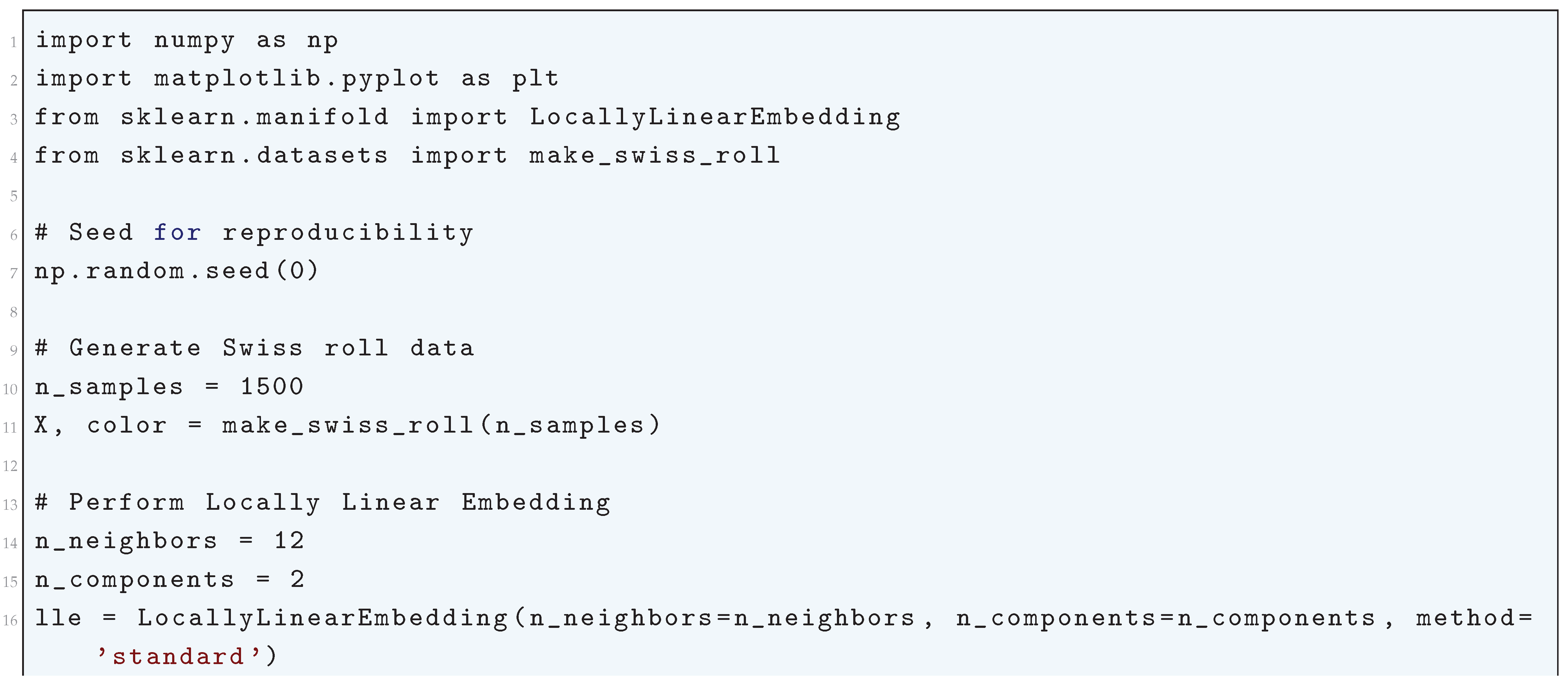
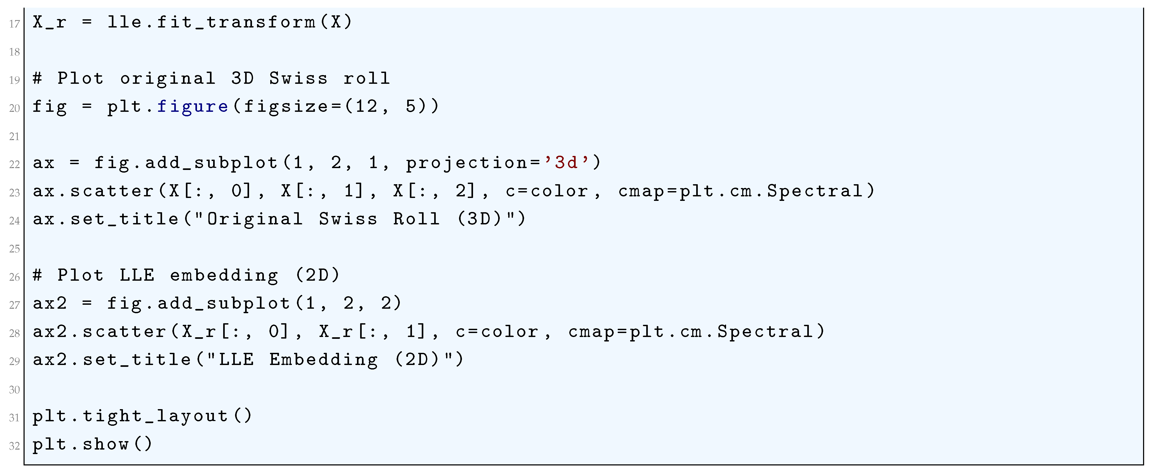
Figure 154.
Locally Linear Embedding (LLE) applied to a Swiss roll dataset. Left: original 3D Swiss roll. Right: 2D LLE embedding preserving local structure
Figure 154.
Locally Linear Embedding (LLE) applied to a Swiss roll dataset. Left: original 3D Swiss roll. Right: 2D LLE embedding preserving local structure
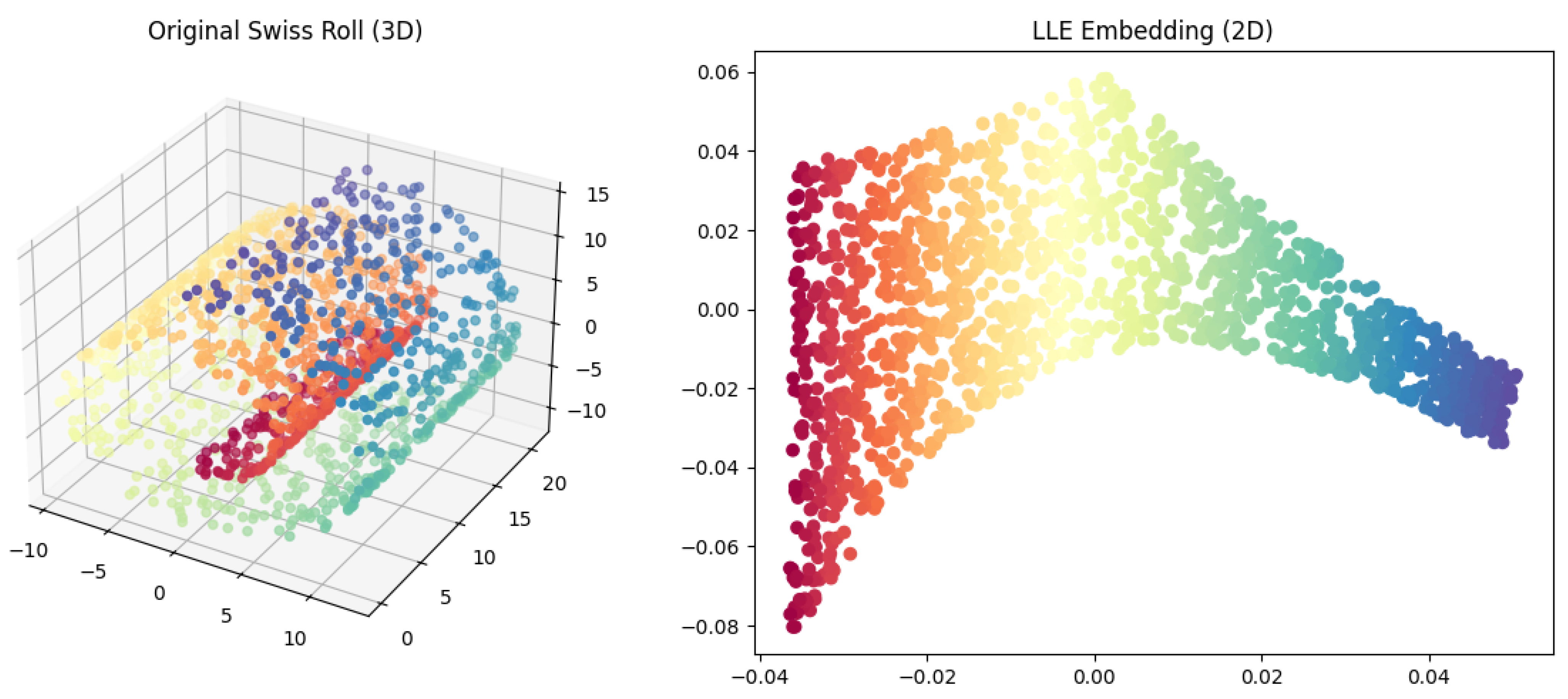
16.1.9. Independent Component Analysis (ICA)
16.1.9.1 Literature Review of Independent Component Analysis (ICA)
Independent Component Analysis (ICA) has developed into a powerful technique in signal processing, statistics, and machine learning. Its theoretical foundations were laid by Comon (1994) [1167], who rigorously introduced the concept of ICA as a method for blind source separation. He provided a detailed mathematical framework, demonstrating how statistical independence, rather than uncorrelatedness, is the key criterion for successful source separation. By linking ICA with higher-order statistics, particularly kurtosis, he established a formal justification for ICA as a generalization of Principal Component Analysis (PCA). This work also introduced the concept of mutual information minimization as a means of achieving independence, offering a theoretical perspective that would influence many later algorithms. Around the same time, Jutten and Herault (1991) [1168] developed an adaptive learning algorithm based on neuromorphic principles, which laid the groundwork for ICA as an iterative computational approach. Their method used nonlinear functions to iteratively adjust the weight matrix, leveraging higher-order statistical moments to achieve source separation, marking one of the first practical implementations of ICA in neural networks.
A major breakthrough came with the development of computationally efficient ICA algorithms, notably the FastICA method by Hyvärinen and Oja (1997) [1169]. They formulated an elegant fixed-point approach that significantly improved the convergence speed of ICA. Instead of using slow gradient-based updates, their method maximized non-Gaussianity using a negentropy approximation, which enabled rapid convergence to independent components. This algorithm incorporated a preprocessing step involving PCA-based whitening, which decorrelated the observed signals before ICA extraction, further enhancing stability and efficiency. In parallel, Bell and Sejnowski (1995) [1044] introduced an information-theoretic approach to ICA, deriving the Infomax algorithm based on maximum likelihood estimation (MLE). Their work established that maximizing the entropy of the output neurons under a nonlinear activation function naturally leads to ICA, providing a fundamental link between ICA and unsupervised neural learning. This insight positioned ICA as a biologically plausible mechanism for sensory processing, particularly in neural coding and vision research.
Several alternative approaches to ICA were also developed, focusing on different statistical principles. Cardoso and Souloumiac (1993) [1170] introduced the JADE algorithm, which employed joint approximate diagonalization of eigenmatrices to separate independent sources. By exploiting fourth-order cumulants, their method avoided gradient descent altogether, leading to a robust and efficient separation procedure, especially for overdetermined mixtures. Meanwhile, Amari et al. (1995) [1171] introduced an ICA algorithm based on natural gradient learning, drawing on concepts from information geometry. They demonstrated that a Riemannian metric on the parameter space of ICA solutions enables more efficient optimization, leading to faster convergence without suffering from the plateaus and slowdowns of traditional gradient descent methods. This information-geometric perspective provided deeper insights into the structure of the ICA optimization landscape and inspired further advances in adaptive ICA algorithms.
A significant refinement of ICA occurred with the extension of Infomax to handle both sub-Gaussian and super-Gaussian source distributions by Lee et al. (1999) [1172]. Their method introduced a nonlinear adaptive function that dynamically adjusted based on the statistical properties of the data, making ICA applicable to a broader range of real-world signals. This extension proved particularly useful in biomedical applications, where sources often exhibit mixed statistical distributions. Around the same time, Pham and Garat (1997) [1173] presented a quasi-maximum likelihood estimation (QMLE) approach to ICA, rigorously formulating the problem as an optimization task within the framework of statistical estimation theory. Their work provided a more systematic theoretical foundation for ICA and improved its robustness in practical scenarios, particularly when dealing with noisy or low-sample data environments.
More recent developments in ICA have explored probabilistic and Bayesian approaches. Højen-Sørensen et al. (2002) [1174] introduced a variational Bayesian framework for ICA, using mean-field approximations to estimate the posterior distribution of independent components. This approach allowed ICA to be extended into a probabilistic setting, making it more robust in the presence of noise and missing data. Their work was particularly influential in applications requiring uncertainty quantification, such as brain imaging and financial modeling. In addition to these algorithmic advancements, Stone (2004) [1175] provided a comprehensive textbook that rigorously detailed the mathematical principles underlying ICA. His work systematically explored the relationship between ICA, mutual information, higher-order statistics, and practical signal processing applications, serving as an authoritative reference for both theoretical research and practical implementation. Together, these contributions have solidified ICA as a fundamental tool in signal processing, machine learning, and neuroscience, with ongoing developments continuing to refine its theoretical underpinnings and expand its applications.
Table 20.
Summary of Contributions in Independent Component Analysis (ICA) Literature
| Authors (Year) | Contribution |
| Comon (1994) [1167] | Established the theoretical framework of ICA, emphasizing statistical independence over uncorrelatedness for blind source separation. Introduced mutual information minimization as a means to achieve independence and linked ICA with higher-order statistics, particularly kurtosis. |
| Jutten and Herault (1991) [1168] | Developed an adaptive learning algorithm for ICA using neuromorphic principles. Introduced nonlinear functions to iteratively adjust the weight matrix based on higher-order statistical moments. This work laid the foundation for iterative computational approaches in ICA. |
| Hyvärinen and Oja (1997) [1169] | Proposed the FastICA algorithm, a fixed-point method maximizing non-Gaussianity using negentropy approximation. Improved convergence speed and incorporated PCA-based whitening for signal decorrelation. |
| Bell and Sejnowski (1995) [1044] | Developed the Infomax algorithm using maximum likelihood estimation, linking ICA to entropy maximization in neural networks. Provided a biological perspective on ICA and its role in sensory processing. |
| Cardoso and Souloumiac (1993) [1170] | Introduced the JADE algorithm, employing joint approximate diagonalization of eigenmatrices to separate independent sources. Used fourth-order cumulants to achieve robust and efficient source separation. |
| Amari et al. (1995) [1171] | Developed an ICA algorithm based on natural gradient learning, utilizing a Riemannian metric for efficient optimization. Provided an information-geometric perspective, improving convergence speed. |
| Lee et al. (1999) [1172] | Extended the Infomax algorithm to handle both sub-Gaussian and super-Gaussian source distributions using a nonlinear adaptive function. Enhanced ICA applicability to biomedical signals with mixed statistical distributions. |
| Pham and Garat (1997) [1173] | Introduced a quasi-maximum likelihood estimation (QMLE) approach to ICA, formulating it as an optimization problem within statistical estimation theory. Improved robustness in noisy and low-sample data environments. |
| Højen-Sørensen et al. (2002) [1174] | Proposed a variational Bayesian framework for ICA using mean-field approximations. Enabled ICA to incorporate uncertainty quantification and handle missing data, extending its robustness. |
| Stone (2004) [1175] | Authored a comprehensive textbook on ICA, detailing its mathematical principles, mutual information, higher-order statistics, and applications in signal processing and machine learning. Provided a systematic exploration of ICA’s theoretical and practical aspects. |
16.1.9.2 Recent Literature Review of Independent Component Analysis (ICA)
Independent Component Analysis (ICA) has found diverse applications across multiple domains, ranging from neuroscience and medical imaging to financial modeling and power systems. Behzadfar et al. (2025) [1176] introduced a novel multi-frequency ICA-based approach to process functional MRI (fMRI) data. Their study focused on extracting meaningful components while effectively removing non-gray matter signals, thereby refining the accuracy of frequency-based brain imaging. The method demonstrated improved signal clarity and more precise voxel-wise frequency difference estimation, making it a valuable tool in neuroimaging research. Similarly, Eierud et al. (2025) [1177] developed the NeuroMark PET ICA framework, which employs ICA to decompose whole-brain PET signals into distinct networks, aiding in the construction of multivariate molecular imaging brain atlases. This technique allows researchers to analyze complex brain connectivity patterns with greater precision, enhancing the study of neurodegenerative disorders and other neurological conditions.
Expanding ICA’s application in hydrology, Wang et al. (2025) [1178] leveraged the technique to analyze terrestrial water storage anomaly (TWSA) trends in the Yangtze River Basin. Their research identified statistically independent spatial trends within hydrological data, offering insights into climate change and its impact on water resource management. By distinguishing significant patterns from background noise, ICA facilitated a more accurate assessment of water distribution and hydrological cycles over time. Similarly, Heurtebise et al. (2025) [1179] used ICA to stabilize estimators in hydrological dataset analysis, improving the reliability of multivariate mutual information measurements. These advancements underscore ICA’s utility in environmental sciences, particularly in large-scale water resource monitoring.
In the field of computational neuroscience, Ouyang and Li (2025) [1180] developed a protocol that integrates ICA with Principal Component Analysis (PCA) for semi-automated EEG preprocessing. Their approach streamlines the removal of artifacts and enhances signal quality, making it easier for researchers to conduct large-scale EEG studies with minimal manual intervention. Zhang and Luck (2025) [1181] further explored ICA’s impact on brain-computer interfaces by assessing the effect of artifact correction on the performance of support vector machine (SVM)-based EEG decoding. Their study demonstrated that ICA-based correction significantly improved classification accuracy, reinforcing its role as a crucial preprocessing tool for neurophysiological data.
ICA has also shown promise in financial modeling and power system monitoring. Kirsten and Süssmuth (2025) [1182] applied ICA to financial time-series data, demonstrating its ability to filter noise and identify independent market-driving factors in cryptocurrency price movements. Their findings indicated that ICA, combined with ARIMA modeling, improved predictive accuracy in highly volatile market environments. Meanwhile, Jung et al. (2025) [1183] developed a hybrid fault detection system that integrates ICA with auto-associative kernel regression (AAKR) for power plant monitoring. Their model effectively isolated independent fault components, enabling more accurate anomaly detection and predictive maintenance strategies.
In signal processing and acoustic applications, Wang et al. (2025) [1184] implemented ICA for noise filtering in passive acoustic localization, particularly for underwater object detection. Their method significantly enhanced the clarity of spatial positioning signals, reducing the impact of environmental noise. Luo et al. (2025) [1185] extended ICA’s utility to brain-computer interfaces (BCIs), where they used the technique to eliminate electrical noise and enhance the transmission of neural signals. Their research demonstrated ICA’s ability to improve the reliability of noninvasive BCIs, paving the way for more accurate and responsive brain-controlled devices.
These studies collectively illustrate ICA’s versatility across disciplines, from improving medical imaging and neurophysiological data analysis to enhancing hydrological assessments, financial forecasting, and fault detection. As ICA continues to evolve, its integration with machine learning techniques and its application in multi-sensor data fusion are likely to expand, offering even greater potential for scientific and industrial advancements. Future research should focus on optimizing ICA algorithms to handle increasingly complex datasets while maintaining computational efficiency.
Table 21.
Summary of Recent Contributions in Independent Component Analysis (ICA) Literature
| Authors (Year) | Contribution |
| Behzadfar et al. (2025) [1176] | Proposed a multi-frequency ICA-based approach for fMRI data processing, enhancing component extraction and eliminating non-gray matter signals for improved frequency-based brain imaging accuracy. |
| Eierud et al. (2025) [1177] | Developed the NeuroMark PET ICA framework, enabling ICA decomposition of whole-brain PET signals into networks to construct multivariate molecular imaging brain atlases. |
| Wang et al. (2025) [1178] | Applied ICA to analyze terrestrial water storage anomaly (TWSA) trends in the Yangtze River Basin, identifying independent spatial trends and improving hydrological cycle assessments. |
| Heurtebise et al. (2025) [1179] | Utilized ICA to stabilize estimators in hydrological dataset analysis, enhancing the reliability of multivariate mutual information measurements. |
| Ouyang and Li (2025) [1180] | Integrated ICA with PCA for semi-automated EEG preprocessing, facilitating artifact removal and improving signal quality in large-scale EEG studies. |
| Zhang and Luck (2025) [1181] | Investigated ICA-based artifact correction in brain-computer interfaces, demonstrating significant improvements in SVM-based EEG decoding accuracy. |
| Kirsten and Süssmuth (2025) [1182] | Applied ICA to financial time-series data, filtering noise and identifying independent market-driving factors, enhancing cryptocurrency price prediction when combined with ARIMA modeling. |
| Jung et al. (2025) [1183] | Developed a hybrid fault detection system integrating ICA with auto-associative kernel regression (AAKR) for power plant monitoring, improving anomaly detection and predictive maintenance. |
| Wang et al. (2025) [1184] | Implemented ICA for noise filtering in passive acoustic localization, significantly enhancing underwater object detection through improved signal clarity. |
| Luo et al. (2025) [1185] | Applied ICA in brain-computer interfaces (BCIs) to eliminate electrical noise and enhance neural signal transmission, improving the reliability of noninvasive BCIs. |
16.1.9.3 Mathematical Analysis of Independent Component Analysis (ICA)
Independent Component Analysis (ICA) is a powerful statistical technique used for blind source separation (BSS), where the goal is to recover a set of statistically independent source signals from their linear mixtures without any prior information about the mixing process. Mathematically, we assume that we are given an n-dimensional observation vector , which is related to an unknown set of source signals through an unknown mixing matrix as follows:
where is the observed signal vector, is the original source vector, and is the mixing matrix that describes how the sources are combined. The objective of ICA is to estimate a demixing matrix such that the transformed signals are as statistically independent as possible:
where ideally , leading to an approximate recovery of the independent source signals. The fundamental assumption that allows ICA to work is that the source signals are statistically independent, meaning their joint probability density function (PDF) factorizes:
This assumption of statistical independence is crucial because it allows the identification of the source signals based on higher-order statistical properties, such as kurtosis and negentropy.
Furthermore, ICA relies on the non-Gaussianity of the source signals, as the central limit theorem (CLT) states that the sum of independent random variables tends toward a Gaussian distribution. Thus, if the sources were Gaussian, they could not be separated from their mixtures because Gaussian distributions are completely characterized by second-order statistics (mean and variance), and higher-order statistics would provide no additional information. To estimate the demixing matrix , we must find a transformation that maximizes the statistical independence of the recovered signals . Several measures of statistical independence exist, including kurtosis, negentropy, and mutual information, which lead to different optimization formulations of ICA. One approach is to use kurtosis, which is defined as the fourth central moment of a random variable:
A Gaussian distribution has a kurtosis of zero, while non-Gaussian distributions have nonzero kurtosis. Since ICA relies on the assumption that the sources are non-Gaussian, we can maximize the absolute value of kurtosis to obtain independent components. Another widely used measure is negentropy, which is derived from information theory and defined as:
where is the differential entropy, given by:
Since entropy measures randomness, negentropy quantifies how far a given distribution is from Gaussianity. The higher the negentropy, the more non-Gaussian the distribution, making it a useful objective function for ICA. An alternative approach is to use mutual information, which measures the statistical dependence between variables:
By minimizing mutual information, we can maximize the statistical independence of the estimated sources. In practical ICA implementations, preprocessing is often necessary to improve performance. A common preprocessing step is whitening, which ensures that the observed signals are uncorrelated and have unit variance. Whitening is achieved by first computing the covariance matrix of :
Performing an eigenvalue decomposition (EVD):
where is the matrix of eigenvectors and is the diagonal matrix of eigenvalues. The whitened signals are then computed as:
This transformation ensures that the covariance of is the identity matrix:
ICA has broad applications in signal processing, including EEG and fMRI signal separation, speech and audio processing, financial time series analysis, and image processing. It is particularly useful in solving the cocktail party problem, where multiple speakers’ voices are separated from mixed audio recordings. The mathematical foundation of ICA makes it one of the most robust techniques for blind signal separation, and its various optimization formulations offer flexibility depending on the application.
16.1.9.4 Python Code to Generate Figure 155 Illustrating the Independent Component Analysis (ICA) of Mixed Signals
The Python code below produces the Figure 155 illustrating the Independent Component Analysis (ICA) of mixed signals.
Figure 155.
Independent Component Analysis (ICA) of mixed signals. The top panel shows mixed signals, the middle panel shows true sources, and the bottom panel shows ICA recovered signals
Figure 155.
Independent Component Analysis (ICA) of mixed signals. The top panel shows mixed signals, the middle panel shows true sources, and the bottom panel shows ICA recovered signals
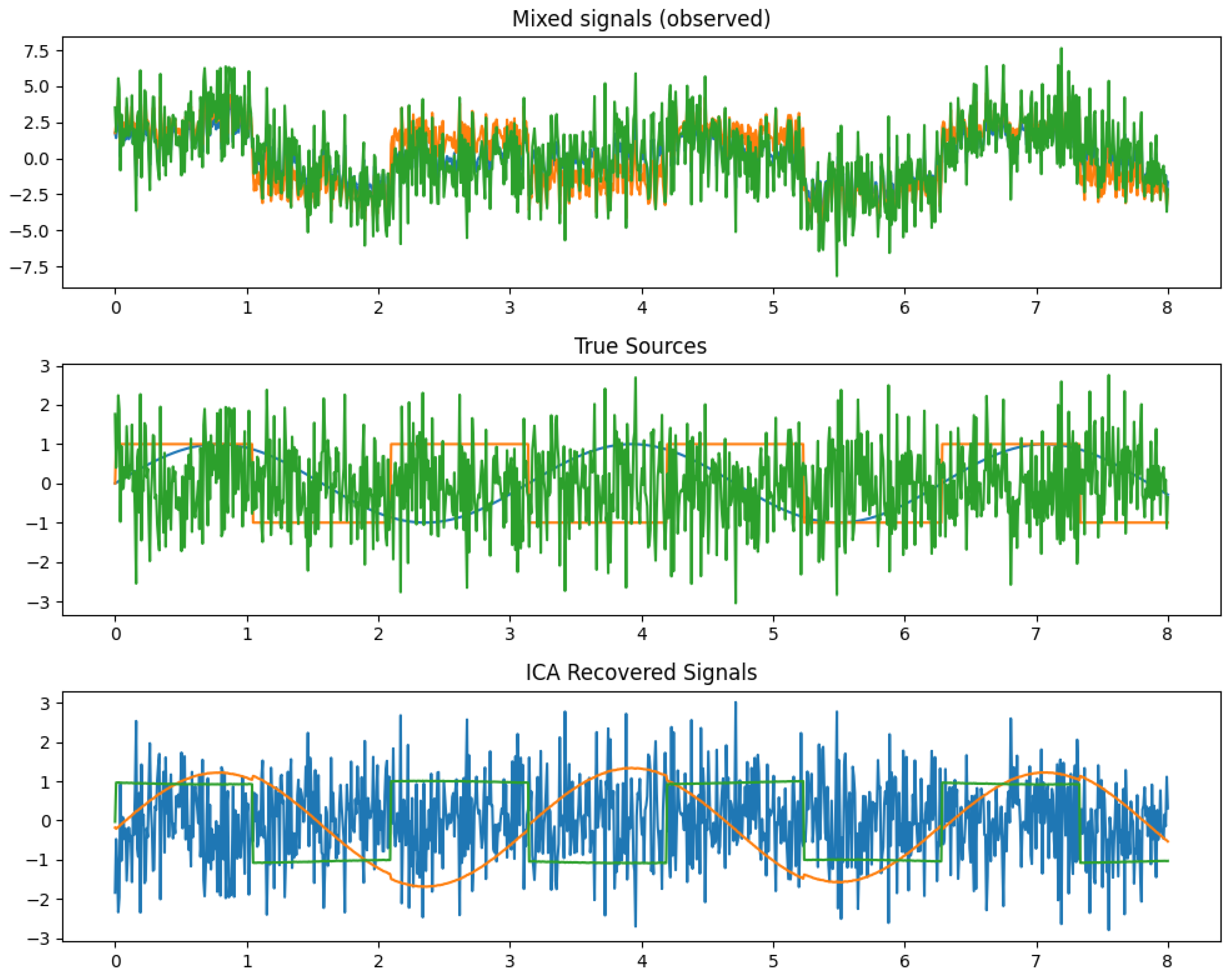
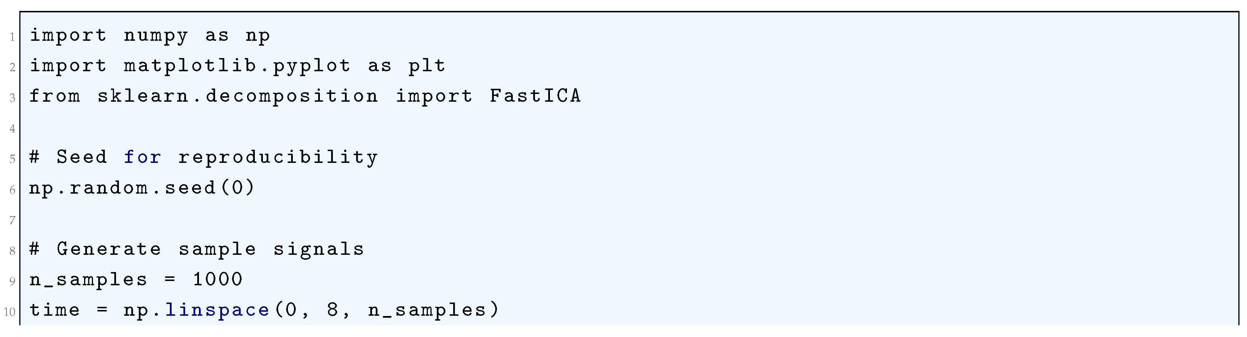
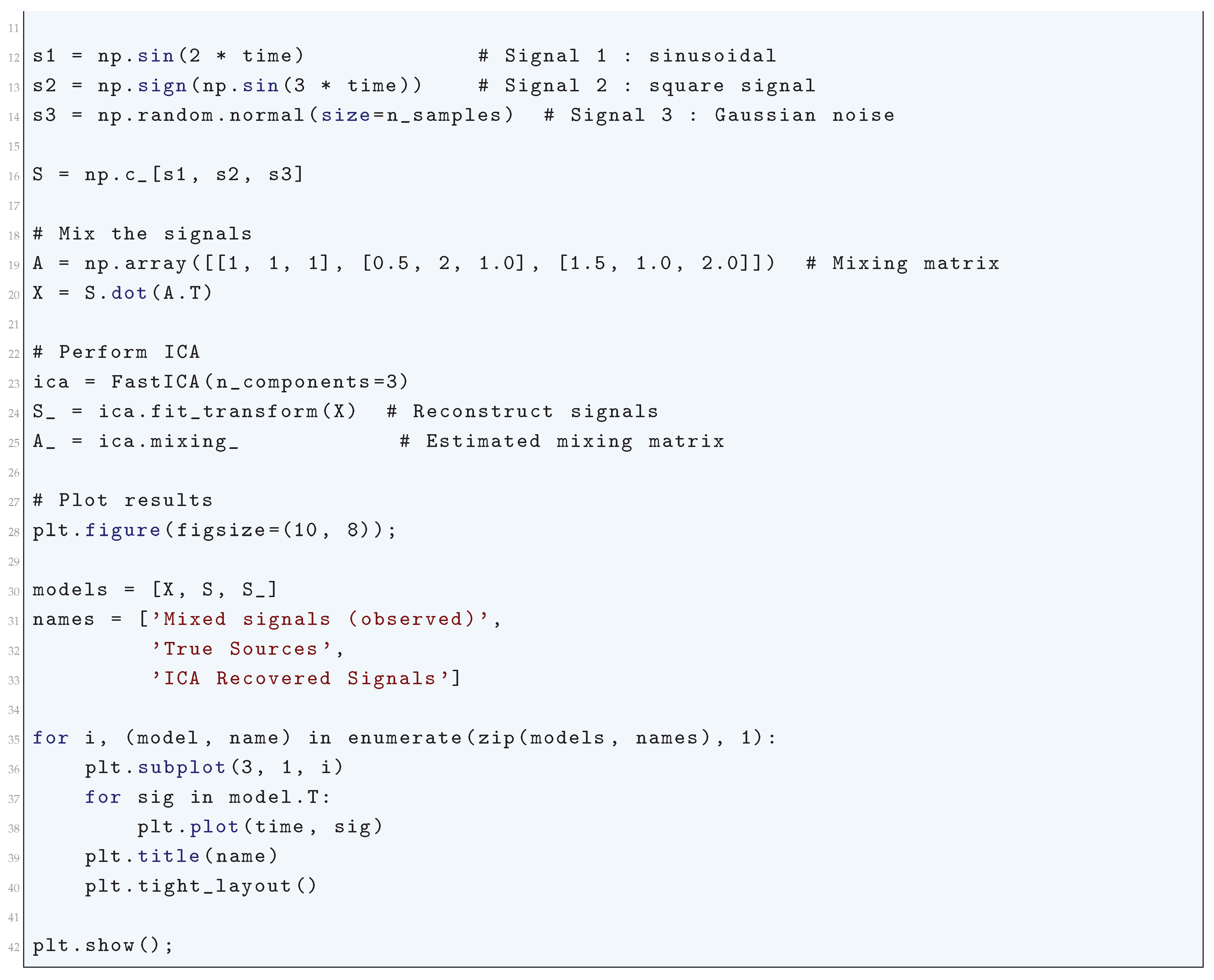
16.2. Supervised Learning
16.2.1. Literature Review of Supervised Learning
Supervised learning has been extensively studied through rigorous theoretical and empirical advancements, forming the backbone of modern machine learning. One of the foundational contributions in this domain is Vapnik (1995) [143], which introduced statistical learning theory, establishing key concepts such as the Vapnik-Chervonenkis (VC) dimension, which quantifies the capacity of a hypothesis class to shatter a given set of data points. The book also presents the principle of structural risk minimization (SRM), which provides a theoretical framework for balancing model complexity and empirical error, thereby preventing overfitting. A critical outcome of this work was the formulation of support vector machines (SVMs), which use kernel functions to transform data into higher-dimensional spaces, enabling the discovery of nonlinear decision boundaries while maintaining strong generalization guarantees. The kernel trick, introduced as a mechanism to implicitly compute inner products in high-dimensional feature spaces, remains one of the most powerful techniques in modern machine learning. Building on statistical foundations, Bishop (2006) [124] provided an extensive treatment of probabilistic models in supervised learning, with a strong emphasis on Bayesian inference. The text rigorously derives Bayesian linear regression, Gaussian processes, and probabilistic neural networks, offering a structured mathematical perspective on uncertainty quantification. The discussion of mixture models and the Expectation-Maximization (EM) algorithm in this work has had profound implications for learning in both supervised and unsupervised settings.
The field of ensemble learning has also seen significant advancements through rigorous mathematical formulations. Breiman (2001) [754] introduced the Random Forest algorithm, an ensemble method based on decision trees, and demonstrated how bootstrap aggregation (bagging) reduces variance in predictive models. The paper provided a theoretical justification for the effectiveness of decorrelating individual decision trees using random feature selection, showing that this mechanism enhances generalization. Moreover, Breiman formally defined the out-of-bag (OOB) error estimation method, an internal validation technique that provides an unbiased estimate of the model’s performance without requiring a separate validation set. Around the same time, Friedman, Hastie, and Tibshirani (2000) [1056] offered a rigorous statistical interpretation of boosting algorithms, particularly AdaBoost. Their work demonstrated that boosting can be understood as a stagewise optimization process that minimizes an exponential loss function, providing a function-space perspective on gradient boosting. By linking boosting to numerical optimization techniques, they laid the foundation for gradient boosting machines (GBMs), which remain one of the most effective supervised learning techniques today. Further theoretical contributions to boosting were made by Schapire (1990) [1058], who formally proved that weak classifiers, which perform only marginally better than random guessing, can be transformed into arbitrarily strong classifiers through the process of boosting. The paper established a precise mathematical framework for analyzing how iterative reweighting of training samples reduces error bounds, reinforcing the statistical robustness of boosting methods.
Deep learning, a subset of supervised learning, has also benefited from rigorous theoretical advancements. LeCun et al. (1998) [1055] introduced convolutional neural networks (CNNs), demonstrating their effectiveness in document recognition, particularly for handwritten digit classification in the MNIST dataset. The authors provided a mathematically rigorous derivation of the backpropagation algorithm and the gradient-based optimization techniques used in training deep networks. One of their major contributions was the concept of weight sharing, which significantly reduces the number of learnable parameters in CNNs by enforcing translational invariance in feature detection. This architecture laid the groundwork for modern deep learning-based vision systems, which have since expanded to complex image recognition tasks. More recently, Srivastava et al. (2014) [141] introduced dropout as a regularization technique for deep neural networks. The authors provided a probabilistic interpretation of dropout as an approximation to model averaging over an exponentially large ensemble of subnetworks, rigorously deriving its impact on reducing overfitting. The paper also presented empirical results demonstrating that dropout significantly improves generalization performance across a wide range of supervised learning tasks.
One of the earliest contributions to supervised learning, which laid the foundation for neural networks, was made by Rosenblatt (1958) [1057] through the introduction of the perceptron algorithm. This work rigorously proved the perceptron convergence theorem, which guarantees that if a dataset is linearly separable, the perceptron learning rule will converge to a separating hyperplane in a finite number of iterations. Although the perceptron was later shown to be limited in expressive power, particularly in its inability to solve non-linearly separable problems such as the XOR problem, it inspired the development of more advanced architectures, including multi-layer perceptrons (MLPs) and deep neural networks. Hastie, Tibshirani, and Friedman (2009) [139] provided one of the most mathematically rigorous treatments of supervised learning, covering a broad range of techniques including linear models, kernel methods, decision trees, ensemble learning, and deep learning. Their work emphasized the mathematical foundations of machine learning, particularly the bias-variance tradeoff, regularization methods such as ridge regression and Lasso, and kernelized learning methods. The authors also provided in-depth theoretical analyses of the convergence properties of various supervised learning algorithms, making their text a fundamental resource for statistical learning theory.
The optimization of deep learning models has been another area of rigorous mathematical research, with Kingma and Ba (2014) [176] introducing the Adam optimization algorithm. Their work provided a detailed mathematical derivation of Adam’s update rules, which rely on the computation of exponentially decaying moving averages of past gradients and squared gradients. The authors rigorously demonstrated how Adam effectively combines the benefits of Adagrad, which adapts learning rates based on the historical sum of squared gradients, and RMSProp, which normalizes updates using an exponentially weighted average of past squared gradients. The method has since become the default optimization algorithm for training deep neural networks, particularly due to its robustness in handling sparse gradients and noisy objective functions. Collectively, these works have profoundly shaped the landscape of supervised learning by introducing mathematically rigorous frameworks for classification, regression, deep learning, and optimization. Their theoretical contributions continue to inform modern advancements, ensuring that machine learning models remain both statistically sound and computationally efficient.
Table 22.
Summary of Contributions in Supervised Learning
| Authors (Year) | Contribution |
| Vapnik (1995) [143] | Introduced statistical learning theory, including the Vapnik-Chervonenkis (VC) dimension, structural risk minimization (SRM), and support vector machines (SVMs). Established the kernel trick for computing inner products in high-dimensional feature spaces. |
| Bishop (2006) [124] | Provided a probabilistic treatment of supervised learning, including Bayesian inference, Gaussian processes, Bayesian linear regression, and probabilistic neural networks. Discussed mixture models and the Expectation-Maximization (EM) algorithm. |
| Breiman (2001) [754] | Introduced Random Forests and bootstrap aggregation (bagging) for variance reduction. Theoretical justification of random feature selection and the out-of-bag (OOB) error estimation method. |
| Friedman, Hastie, and Tibshirani (2000) [1056] | Provided a statistical interpretation of boosting, demonstrating its connection to stagewise optimization of an exponential loss function. Established the foundation for gradient boosting machines (GBMs). |
| Schapire (1990) [1058] | Proved that weak classifiers can be transformed into strong classifiers through boosting. Developed a mathematical framework for iterative sample reweighting to reduce error bounds. |
| LeCun et al. (1998) [1055] | Introduced convolutional neural networks (CNNs) with applications to handwritten digit recognition. Provided rigorous derivations of backpropagation and weight sharing for reducing parameters. |
| Srivastava et al. (2014) [141] | Proposed dropout as a regularization technique in deep learning, providing a probabilistic interpretation as model averaging. Demonstrated improvements in generalization performance. |
| Rosenblatt (1958) [1057] | Introduced the perceptron algorithm and proved the perceptron convergence theorem for linearly separable data. Inspired the development of multi-layer perceptrons (MLPs) and deep networks. |
| Hastie, Tibshirani, and Friedman (2009) [139] | Provided a rigorous mathematical treatment of supervised learning, including regularization methods (ridge regression, Lasso), bias-variance tradeoff, kernel methods, decision trees, and ensemble learning. Theoretical analyses of algorithm convergence properties. |
| Kingma and Ba (2014) [176] | Developed the Adam optimization algorithm, combining Adagrad and RMSProp principles. Provided a mathematical derivation of Adam’s update rules for adaptive learning rates in deep learning models. |
16.2.2. Recent Literature Review of Supervised Learning
Supervised learning has found extensive applications across multiple domains, enhancing decision-making, classification, and predictive analytics through well-labeled datasets. Raikwar and Gupta (2025) [1046] developed an AI-driven trust management framework that integrates both supervised and unsupervised learning to classify security levels in wireless ad hoc networks. Their model improves the robustness of decentralized communication by leveraging machine learning-based trust computation, enhancing the detection of malicious nodes and mitigating vulnerabilities in self-organizing networks. Similarly, Rafiei et al. (2025) [1059] employed supervised multi-output classification models, including Random Forest and Support Vector Machines, to optimize lipid nanoparticle design for mRNA delivery. Their research demonstrates how machine learning can refine drug formulation by predicting the best combination of lipid components to enhance delivery efficiency. This showcases the growing role of supervised learning in biotechnology and precision medicine.
In the field of remote sensing and agriculture, Pei et al. (2025) [1060] introduced a weakly supervised learning approach for segmenting vegetation from UAV images. Traditional supervised models often struggle with limited labeled datasets in complex outdoor environments, but their model incorporates spectral reconstruction techniques to improve classification accuracy in field conditions. This advancement significantly enhances agricultural monitoring and precision farming. Likewise, Efendi et al. (2025) [1061] designed an IoT-based health monitoring system where supervised learning algorithms were used to classify and predict health anomalies in elderly patients. Their study highlights how cloud computing and machine learning can be combined to provide real-time health insights, ultimately enabling better remote patient care.
Another critical challenge in supervised learning is the scarcity of labeled data, which was addressed by Pang et al. (2025) [1062] in their research on protein transition pathway prediction. They introduced DeepPath, a framework that integrates active learning with supervised deep learning, allowing models to efficiently identify uncertain data points for labeling. This method enhances model accuracy while reducing the dependency on extensive labeled datasets, making it particularly useful for complex biological simulations. In a different application, Curry et al. (2025) [1063] explored supervised classification techniques in geoscience, comparing their effectiveness with unsupervised clustering methods for analyzing ignimbrite flare-up patterns. Their work provides insights into how machine learning models can be optimized for geological pattern detection, improving hazard assessment and geological forecasting.
In the realm of computational drug discovery, Li et al. (2025) [1064] developed a deep learning-based framework called -PhenoDrug, which employs supervised learning for phenotypic drug screening. The model utilizes transfer learning strategies and neural networks to classify drug interactions, significantly accelerating the identification of promising drug candidates. Similarly, Liu et al. (2025) [1065] integrated supervised learning with molecular docking and dynamic simulations to identify ASGR1 and HMGCR dual-target inhibitors. By combining computational chemistry with machine learning, they were able to streamline the drug discovery process, demonstrating the efficiency of supervised models in pharmaceutical research. These contributions highlight the transformative potential of supervised learning in biomedical applications.
Beyond healthcare and science, supervised learning is also playing a crucial role in business and engineering. Dutta and Karmakar (2025) [1067] investigated the application of the Random Forest algorithm in business analytics, demonstrating its superior accuracy in predictive modeling compared to other machine learning approaches. Their findings illustrate how machine learning can optimize decision-making processes in organizational contexts. Finally, Ekanayake (2025) [1054] explored the use of supervised deep learning models for enhancing Magnetic Resonance Imaging (MRI) reconstruction and super-resolution. Their study addresses the challenges of lengthy MRI scan times by leveraging artificial intelligence to improve image quality, thereby advancing medical diagnostics and reducing patient discomfort.
These studies collectively demonstrate the broad impact of supervised learning across various disciplines, from security and healthcare to remote sensing, drug discovery, and business analytics. The integration of machine learning with domain-specific challenges has led to significant breakthroughs, highlighting the adaptability and efficiency of supervised learning models. As researchers continue to refine these techniques, the future of artificial intelligence-driven decision-making appears increasingly promising. The ability of supervised learning to extract meaningful patterns from structured data is proving invaluable in solving real-world problems, paving the way for further advancements in machine learning research and its practical applications.
Table 23.
Summary of Recent Contributions in Supervised Learning
| Authors (Year) | Contribution |
| Raikwar and Gupta (2025) [1046] | Developed an AI-driven trust management framework integrating supervised and unsupervised learning to classify security levels in wireless ad hoc networks. Enhanced decentralized communication robustness and improved detection of malicious nodes. |
| Rafiei et al. (2025) [1059] | Applied supervised multi-output classification models, including Random Forest and SVMs, to optimize lipid nanoparticle design for mRNA delivery, improving drug formulation predictions. |
| Pei et al. (2025) [1060] | Proposed a weakly supervised learning approach for segmenting vegetation from UAV images, enhancing classification accuracy in precision farming. |
| Efendi et al. (2025) [1061] | Designed an IoT-based health monitoring system that uses supervised learning algorithms to classify and predict health anomalies in elderly patients, improving remote patient care. |
| Pang et al. (2025) [1062] | Introduced DeepPath, a supervised deep learning framework integrating active learning for protein transition pathway prediction, reducing dependency on extensive labeled datasets. |
| Curry et al. (2025) [1063] | Compared supervised classification techniques and unsupervised clustering in geoscience, optimizing machine learning models for geological pattern detection and hazard assessment. |
| Li et al. (2025) [1064] | Developed -PhenoDrug, a deep learning-based framework employing supervised learning for phenotypic drug screening, accelerating drug candidate identification. |
| Liu et al. (2025) [1065] | Integrated supervised learning with molecular docking and simulations to identify ASGR1 and HMGCR dual-target inhibitors, streamlining drug discovery. |
| Dutta and Karmakar (2025) [1067] | Investigated Random Forest applications in business analytics, demonstrating superior predictive modeling accuracy for optimizing organizational decision-making. |
| Ekanayake (2025) [1054] | Applied supervised deep learning models to enhance MRI reconstruction and super-resolution, improving medical diagnostics by reducing scan times. |
16.2.3. Mathematical Analysis of Supervised Learning
Supervised learning is a fundamental paradigm in machine learning wherein a model is trained using labeled data, consisting of input-output pairs . Here, represents the feature vector of the ith data point, and represents the corresponding label, which can be either continuous (regression) or discrete (classification). The goal of supervised learning is to learn a function or such that for an unseen input , the model produces an accurate prediction . Mathematically, the model aims to approximate the conditional probability distribution , i.e.,
where the expectation is taken with respect to the true underlying data distribution . The optimal function minimizes the expected loss over the data distribution,
where denotes the hypothesis space of functions and is a loss function quantifying the error between the true and predicted values.
In empirical risk minimization (ERM), the expectation is approximated using the training set, leading to
For regression tasks, common choices for include the squared loss,
which leads to the minimization of the mean squared error (MSE),
For classification, a frequently used loss function is the cross-entropy loss for a model outputting class probabilities ,
where K is the number of classes and is the indicator function that is 1 if and 0 otherwise. The classifier aims to minimize the empirical risk,
To optimize , gradient-based methods are commonly used, particularly in deep learning where f is parameterized by a neural network with weights ,
where and are weight matrices and bias vectors at layer l, and is an activation function. The optimization process follows stochastic gradient descent (SGD), updating parameters iteratively as follows,
where is the learning rate and is the loss function. The gradient is computed via backpropagation,
Regularization techniques, such as L2 regularization (ridge regression),
are used to prevent overfitting by penalizing large weights. In logistic regression, the probability of a binary label is modeled using the sigmoid function,
The loss function in this case is the binary cross-entropy loss,
Thus, supervised learning encompasses various frameworks, each employing rigorous mathematical formulations to optimize predictive performance.
16.2.4. Python Code to Generate Figure 156 Illustrating the Supervised Learning in Regression
The Python code below produces the Figure 156 illustrating the Supervised Learning in Regression.
Figure 156.
Illustration of Supervised Learning in regression. Blue points represent training data, the dashed green line is the true underlying function, and the red line is the model learned from data
Figure 156.
Illustration of Supervised Learning in regression. Blue points represent training data, the dashed green line is the true underlying function, and the red line is the model learned from data
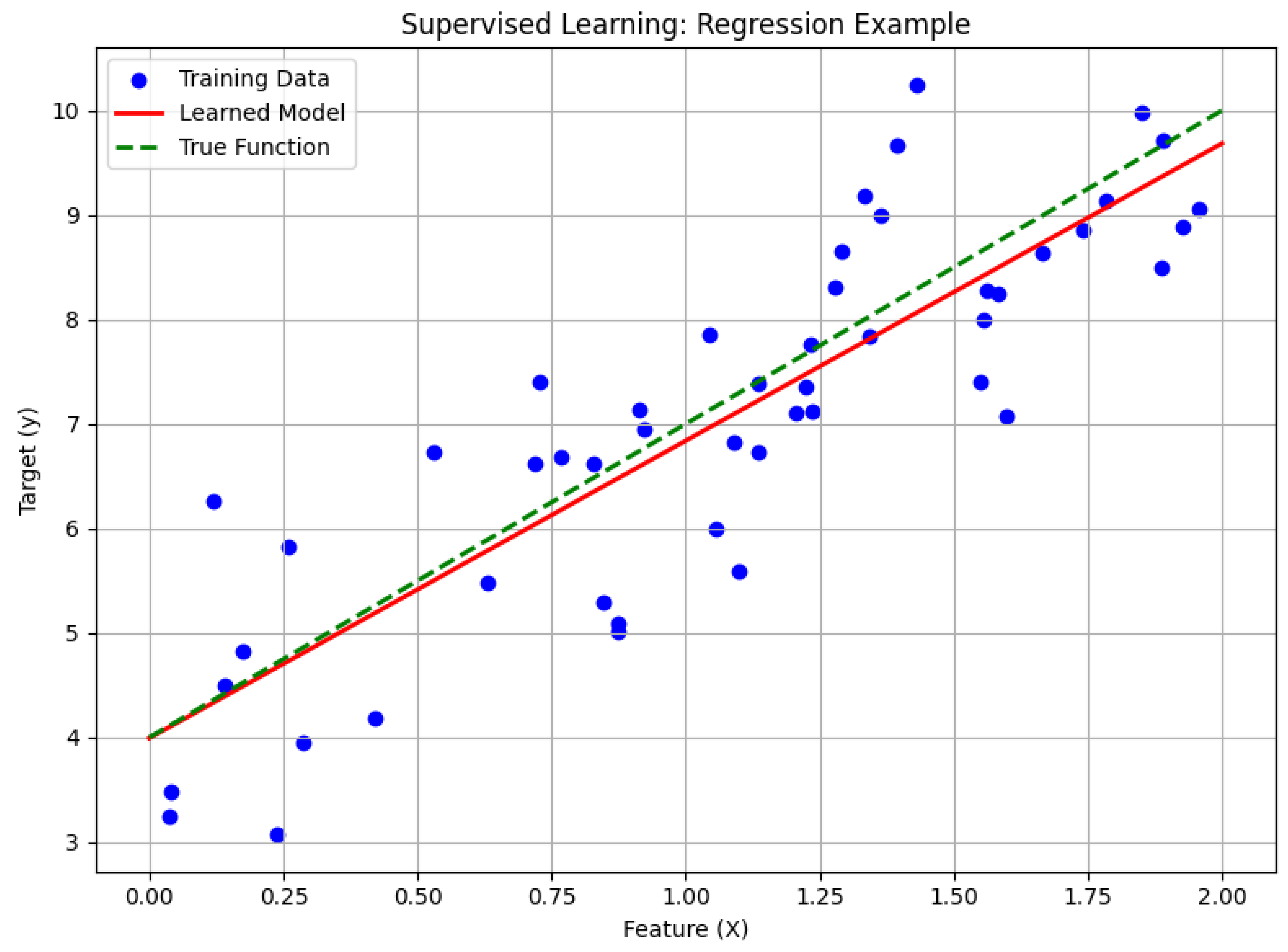
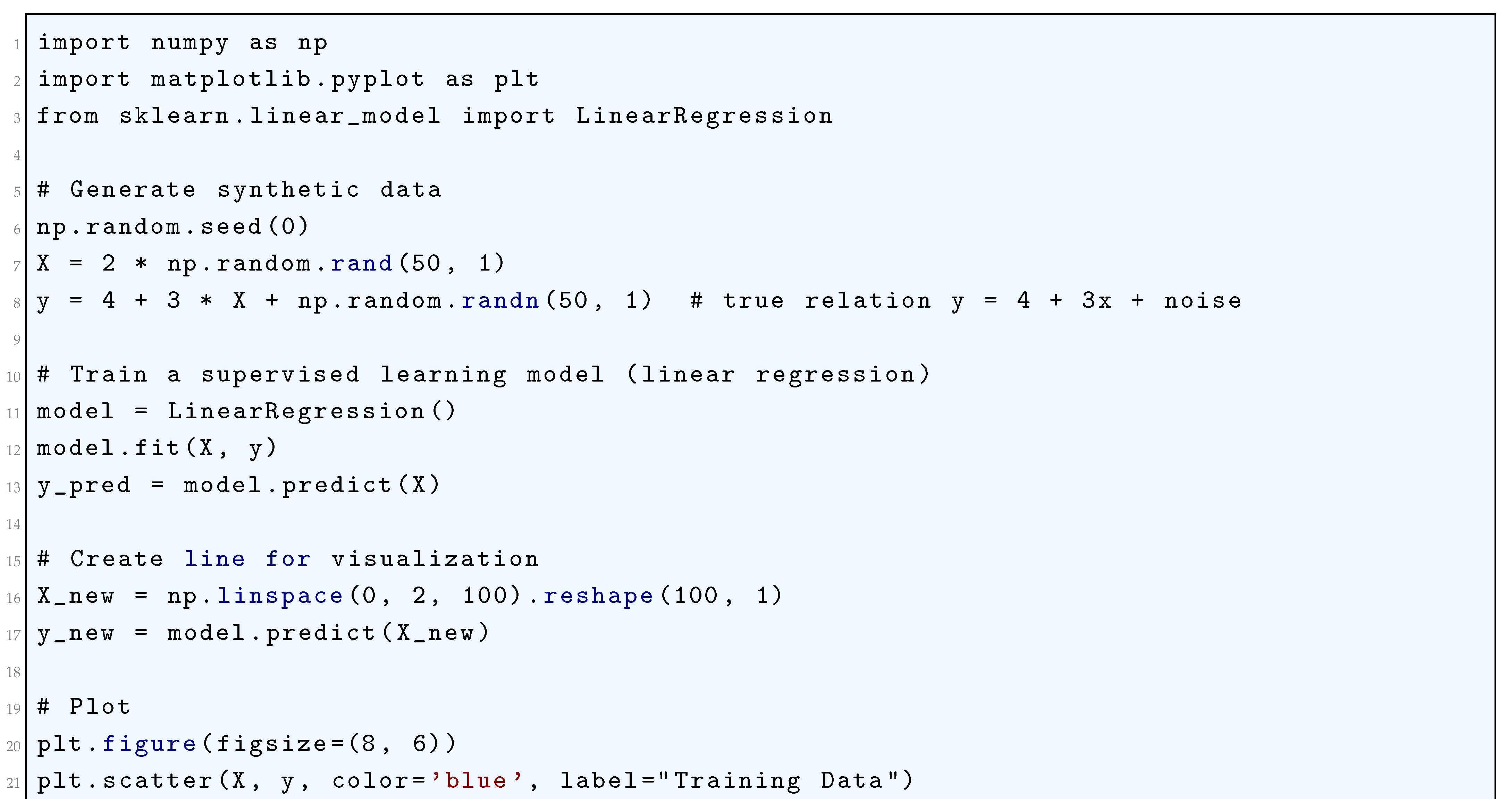
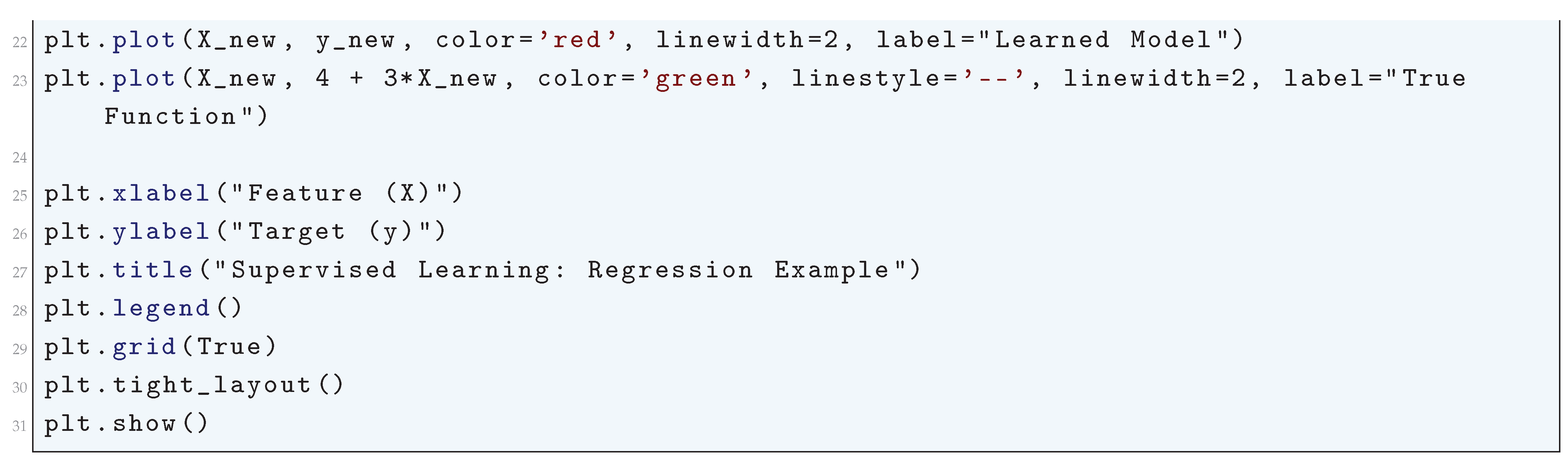
16.2.5. Bias-Variance Tradeoff of Supervised Learning
16.2.5.1 Literature Review of Bias-Variance Tradeoff of Supervised Learning
The bias-variance tradeoff is a crucial concept in supervised learning, dictating how model complexity impacts predictive performance. Geman, Bienenstock, and Doursat (1992) [882] introduced the bias-variance decomposition in the context of neural networks, rigorously establishing that overly simple models suffer from high bias due to underfitting, while excessively complex models exhibit high variance due to overfitting. This foundational work provided a theoretical framework that has guided decades of machine learning research. Hastie, Tibshirani, and Friedman (2001) [139] further expanded upon this concept in their comprehensive textbook, where they provided mathematical formulations, empirical analyses, and practical implications of the tradeoff across various learning algorithms. Their work remains one of the most widely referenced sources for understanding the balance between bias and variance in real-world applications. More recently, Belkin et al. (2019) [883] challenged the classical understanding of the tradeoff by introducing the "double descent" risk curve, demonstrating that in highly over-parameterized models, test error initially increases but eventually decreases beyond a critical complexity threshold. This counterintuitive result, grounded in empirical evidence and theoretical analysis, reshaped the conventional wisdom regarding model selection and generalization in modern machine learning.
In the context of deep learning, Neal et al. (2018) [884] revisited the bias-variance tradeoff, rigorously analyzing why larger neural networks often achieve superior generalization despite their over-parameterization. They argued that implicit regularization, induced by optimization algorithms such as stochastic gradient descent, plays a crucial role in preventing excessive variance growth. Rocks and Mehta (2020) [885] further investigated over-parameterized models using statistical physics methods, deriving explicit analytical expressions for bias and variance in settings such as linear regression and shallow neural networks. Their work provided a deeper theoretical understanding of how interpolation affects generalization, revealing a phase transition where the training error collapses to zero while test error exhibits non-trivial behavior due to the complex interaction of bias and variance. Meanwhile, Doroudi and Rastegar (2023) [886] extended the bias-variance framework beyond machine learning, applying it to cognitive science models. Their work emphasized that cognitive processes also operate under similar tradeoffs, where overly rigid or overly flexible models fail to accurately capture human learning and reasoning, thereby providing an interdisciplinary perspective on the problem.
The practical implications of the bias-variance tradeoff extend to domains such as label noise, knowledge distillation, and ensemble learning. Almeida et al. (2020) [887] focused on mitigating class boundary label uncertainty, proposing an approach that estimates label noise and adjusts training sample weights to simultaneously reduce both bias and variance. Their method provided empirical evidence that accounting for uncertainty near decision boundaries leads to improved generalization performance. Zhou et al. (2021) [888] explored the role of soft labels in knowledge distillation, demonstrating that these labels act as a form of implicit regularization that influences the bias-variance tradeoff in student-teacher learning paradigms. They proposed a novel method of weighting soft labels to dynamically balance bias and variance at the sample level. Gupta et al. (2022) [889] examined ensemble methods from a bias-variance perspective, showing that ensembling reduces variance without significantly increasing bias. Their theoretical and empirical results highlighted why ensemble-based approaches often outperform single models in practice. Finally, Ranglani (2024) [890] conducted an extensive empirical analysis across different machine learning algorithms, quantifying the bias-variance decomposition and providing insights into the tradeoff dynamics in regression and classification tasks. Their study offered practical guidelines for optimizing machine learning models by rigorously understanding how bias and variance manifest across various architectures.
Collectively, these works illustrate the evolution of the bias-variance tradeoff from its classical roots to its modern reinterpretation in deep learning and beyond. They provide rigorous theoretical insights and empirical validations that have fundamentally shaped the field of machine learning. The contributions span diverse perspectives, from statistical learning theory to interdisciplinary applications, and challenge traditional notions of model complexity and generalization. The continued exploration of this tradeoff remains a central theme in machine learning research, influencing advancements in algorithm design, optimization techniques, and real-world deployment strategies.
Table 24.
Summary of Contributions to the Bias-Variance Tradeoff in Supervised Learning
| Reference | Contribution |
| Geman, Bienenstock, and Doursat (1992) | Introduced the bias-variance decomposition in neural networks, demonstrating how model complexity influences predictive error. They formulated a theoretical framework explaining the tradeoff between underfitting (high bias) and overfitting (high variance). |
| Hastie, Tibshirani, and Friedman (2001) | Provided a comprehensive treatment of the bias-variance tradeoff in statistical learning, including rigorous mathematical derivations, practical insights, and empirical analyses across multiple machine learning models. |
| Belkin et al. (2019) | Challenged the classical U-shaped bias-variance curve by introducing the "double descent" phenomenon, showing that over-parameterized models can exhibit improved generalization after an initial increase in test error. |
| Neal et al. (2018) | Analyzed the bias-variance tradeoff in deep learning, arguing that implicit regularization induced by stochastic gradient descent prevents excessive variance growth in large neural networks, explaining their surprising generalization ability. |
| Rocks and Mehta (2020) | Derived analytical expressions for bias and variance in over-parameterized models using statistical physics, uncovering a phase transition where increasing model complexity leads to test error reduction despite interpolation. |
| Guest and Martin (2021) | Extended the bias-variance framework to cognitive science, demonstrating how cognitive models suffer from similar tradeoffs between flexibility and generalization. They argued that model complexity in human cognition follows analogous patterns. |
| Almeida et al. (2020) | Developed a method for mitigating label uncertainty near class boundaries, proposing an adaptive weighting mechanism to reduce both bias and variance, thereby improving model generalization. |
| Zhou et al. (2021) | Investigated knowledge distillation through the lens of the bias-variance tradeoff, demonstrating that soft labels act as implicit regularizers and proposing an optimal weighting scheme to balance bias and variance at the sample level. |
| Gupta et al. (2022) | Provided a rigorous analysis of ensemble methods, proving that ensembling reduces variance without substantially increasing bias, explaining why ensemble learning consistently outperforms single-model approaches. |
| Ranglani (2024) | Conducted an extensive empirical study of the bias-variance tradeoff across various supervised learning models, quantifying bias and variance components and offering practical guidelines for model optimization. |
16.2.5.2 Recent Literature Review of Bias-Variance Tradeoff of Supervised Learning
The bias-variance tradeoff is a fundamental concept in supervised learning, balancing model complexity and generalization performance. Recent literature explores its implications across various domains, including classical statistical learning, deep learning, and ensemble methods. Rahman and Rahman (2024) provide a foundational overview, discussing its role in linear classifiers and logistic regression, where regularization is used to mitigate overfitting. Tran et al. (2024) extend this idea to power systems, demonstrating how a learnable weighted-ensemble neural network optimally manages the tradeoff, particularly in handling real-world power flow optimization. Similarly, George (2024) examines how bias-variance adjustments impact handwriting recognition using the Kaggle digits dataset, emphasizing the importance of tuning model complexity for improved character classification accuracy.
In the context of statistical modeling, Polson and Sokolov (2024) rigorously analyze hierarchical linear models, showcasing how ridge and lasso regression act as regularization techniques to minimize variance while maintaining sufficient flexibility to prevent high bias. This is further explored by Jogo (2025), who provides a broader statistical perspective, linking the bias-variance tradeoff to support vector machines, unsupervised learning, and computational efficiency in high-dimensional spaces. Additionally, Du et al. (2025) introduce a mathematical framework that incorporates margin theory and optimization-based strategies to manage bias-variance tradeoffs in ensemble learning, highlighting computational trade-offs associated with different model architectures.
A particularly interesting development in deep learning is the challenge to the traditional U-shaped bias-variance curve, as presented by Wang and Pope (2025). Their work on the double descent phenomenon suggests that increasing model complexity beyond a certain threshold can actually improve generalization, contradicting classical theory. In a related vein, Chen et al. (2024) investigate the role of graph convolutional networks in regression tasks, providing a theoretical framework to understand how different convolutional layers impact the bias-variance tradeoff. Meanwhile, Obster et al. (2024) take a more interpretability-focused approach, proposing a scoring system to balance predictive accuracy and model transparency while managing the bias-variance relationship.
Finally, ensemble-based techniques continue to be a crucial area of exploration in mitigating bias-variance issues. Owen et al. (2024) revisit bagging and stochastic algorithms, extending the bias-variance decomposition to demonstrate how ensemble methods enhance generalization. Their work aligns with recent trends advocating for hybrid model selection strategies that optimize variance reduction without sacrificing interpretability. The collective findings of these studies underscore the evolving nature of the bias-variance tradeoff in supervised learning, from classical statistical interpretations to novel deep learning insights, and highlight its persistent influence on model performance across diverse applications.
| Reference | Summary of Contribution |
| Rahman & Rahman (2024) | Provides a foundational introduction to the bias-variance tradeoff in machine learning, focusing on logistic regression, linear classifiers, and regularization techniques. Discusses how adjusting model complexity impacts generalization performance. |
| Tran, Mitra, & Nguyen (2024) | Explores how an ensemble-based neural network effectively balances the bias-variance tradeoff in power system optimization. Demonstrates the model’s ability to enhance stability and accuracy in real-world energy distribution scenarios. |
| George (2024) | Investigates how different machine learning models handle the bias-variance tradeoff in character recognition. Uses the Kaggle digits dataset to optimize performance through regularization and model selection strategies. |
| Du et al. (2025) | Develops a theoretical framework linking bias-variance tradeoff to margin theory and optimization techniques. Proposes computational trade-offs to improve model selection in ensemble learning methods. |
| Polson & Sokolov (2024) | Explains the role of ridge and lasso regression in controlling the bias-variance tradeoff. Provides empirical studies demonstrating how hyperparameter tuning influences model performance and generalization. |
| Jogo (2025) | Covers the statistical foundations of the bias-variance tradeoff, linking it to support vector machines, unsupervised learning, and computational efficiency in high-dimensional spaces. |
| Wang & Pope (2025) | Challenges the traditional U-shaped bias-variance tradeoff by showing that increased complexity beyond a certain point can improve generalization in deep learning models. |
| Chen, Schmidt-Hieber, & Donnat (2024) | Analyzes the impact of graph convolutional networks (GCNs) on bias-variance tradeoff, providing a theoretical framework for evaluating convolutional layer depth in regression models. |
| Obster, Ciolacu, & Humpe (2024) | Investigates the tradeoff between predictive accuracy and interpretability in machine learning models. Introduces a scoring system for model complexity optimization while maintaining an optimal bias-variance balance. |
| Owen, Dick, & Whigham (2024) | Extends the bias-variance decomposition for stochastic learning algorithms, demonstrating how bagging-based ensemble methods improve generalization. Highlights hybrid model selection strategies for variance reduction. |
16.2.5.3 Mathematical Analysis of Bias-Variance Tradeoff of Supervised Learning
In supervised learning, the bias-variance tradeoff is a fundamental concept that governs the performance of a model in terms of its ability to generalize to unseen data. Mathematically, the total expected error of a model, often measured as the mean squared error (MSE), can be decomposed as follows:
where Y is the true response variable, X is the input feature, is the true underlying function, and is the estimated function learned by the model. The decomposition highlights three key sources of error:
- Bias: This term quantifies how far the expected prediction is from the true function . Formally, it is defined asA high-bias model makes systematic errors because it fails to capture the complexity of the data. This often occurs in underfitting, where the model is too simple to represent the underlying structure of the data.
- Variance: This term quantifies the variability of the model’s predictions around its expected value, given byA high-variance model is highly sensitive to fluctuations in the training data and does not generalize well to unseen data. This typically occurs in overfitting, where the model captures noise instead of the true signal.
- Irreducible Error: The term represents noise inherent in the data that no model can eliminate.
Since the total error is the sum of these components, an increase in one term often leads to a decrease in another.
For instance, using a more flexible model (e.g., a high-degree polynomial) can reduce bias but at the cost of increased variance. Conversely, using a simple model (e.g., linear regression) reduces variance but increases bias. This tradeoff is captured by minimizing the expected loss function
where the goal is to balance the bias and variance terms to achieve optimal generalization. To analyze this tradeoff further, consider a simple linear model where the target function is quadratic:
If we fit a linear regression model , then the bias is
For a high-degree polynomial model , the variance term increases with d, leading to:
Minimizing the expected generalization error requires selecting a model complexity d such that
To further illustrate, consider a dataset of size n and a model parameterized by . The variance of the estimator is given by
whereas the bias squared is
The total mean squared error (MSE) of the estimator is then
As the complexity of the model increases, the bias decreases, but variance increases. This behavior is described by the function
where are constants depending on the dataset and learning algorithm, and d represents model complexity. The optimal complexity satisfies
For neural networks, increasing the number of layers and neurons often leads to decreased bias but significantly increased variance due to overparameterization. The expected loss for a neural network with weights W trained on data is given by
Regularization techniques such as ridge regression introduce a penalty term , leading to the optimization problem
This reduces variance at the cost of increasing bias, effectively controlling model complexity to achieve an optimal bias-variance tradeoff.
16.2.5.4 Python Code to Generate Figure 157 Illustrating the Bias-Variance Tradeoff of Supervised Learning
The Python code below produces the Figure 157 illustrating the Bias-Variance Tradeoff of Supervised Learning.
Figure 157.
Bias-Variance Tradeoff in Supervised Learning. Bias2 decreases with model complexity, variance increases, training error decreases, and test error initially decreases then increases due to overfitting
Figure 157.
Bias-Variance Tradeoff in Supervised Learning. Bias2 decreases with model complexity, variance increases, training error decreases, and test error initially decreases then increases due to overfitting
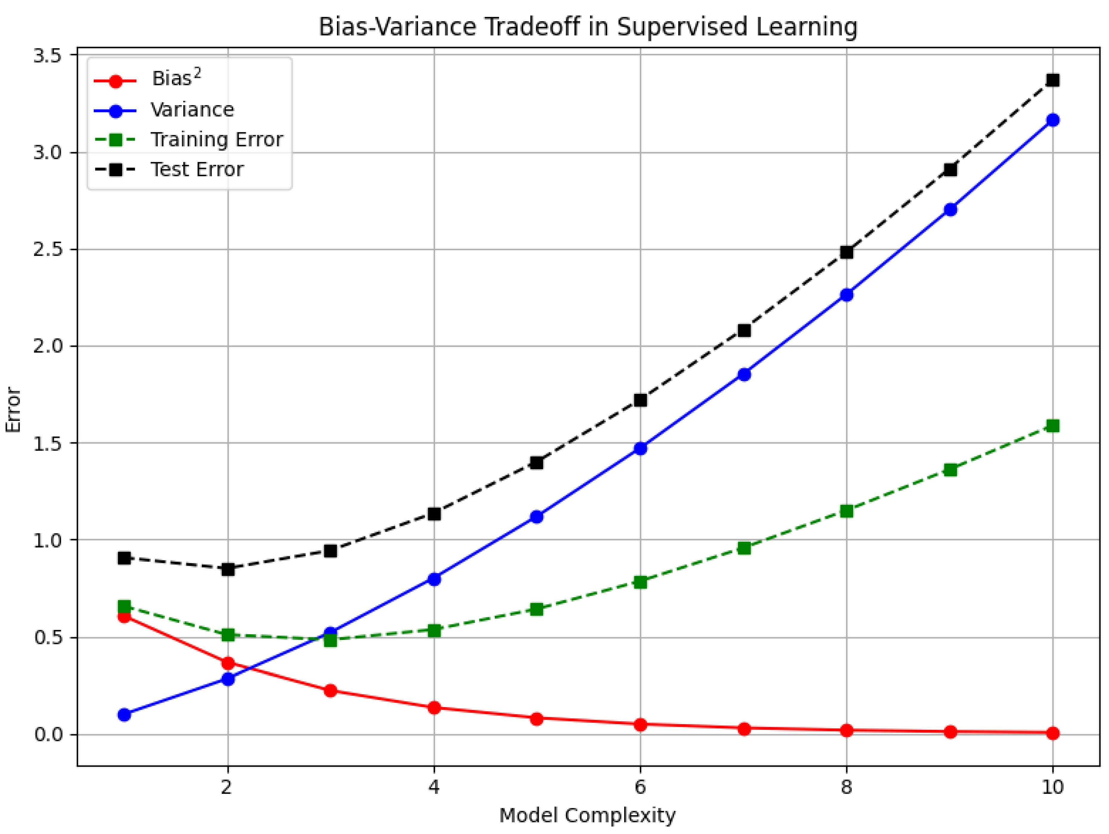
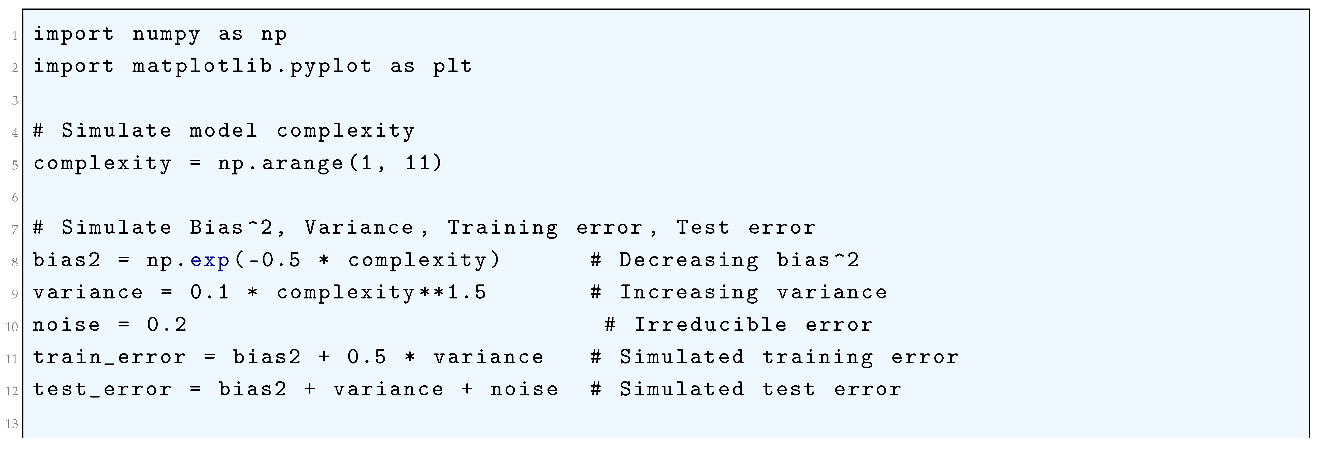
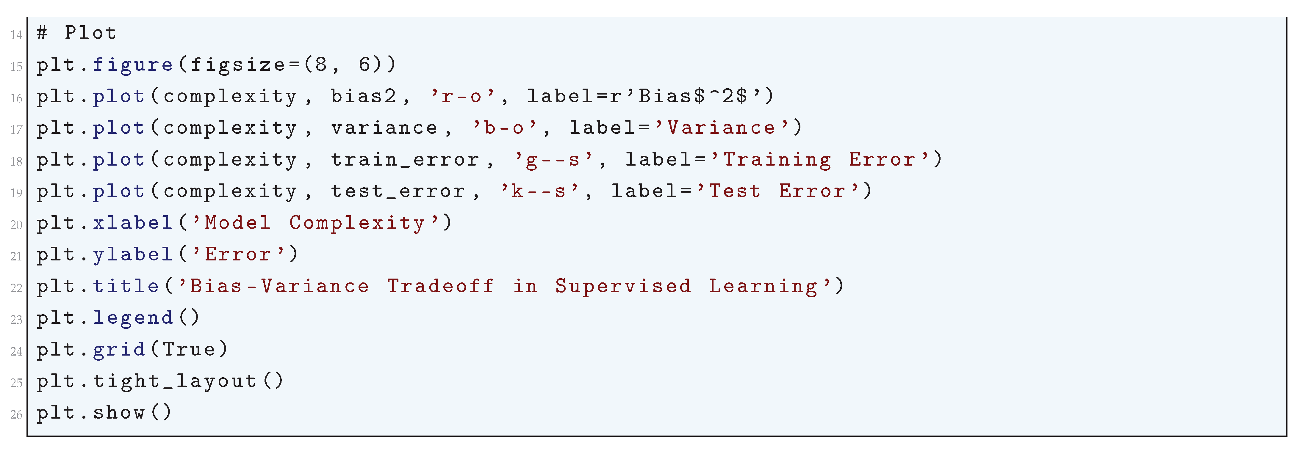
16.2.6. Support Vector Machine
16.2.6.1 Literature Review of Support Vector Machine
Support Vector Machines (SVMs) are rooted in Vladimir Vapnik’s “The Nature of Statistical Learning Theory" (1995) [143], which introduced the fundamental principle of structural risk minimization (SRM). Unlike empirical risk minimization, which solely minimizes training error, SRM aims to balance the complexity of the model and its ability to generalize to unseen data, thereby preventing overfitting. This theoretical framework laid the foundation for the development of SVMs as a powerful tool for classification and regression problems. Schölkopf and Smola’s "Learning with Kernels" (2002) [823] provided a mathematically rigorous treatment of kernel methods, which form the core of SVMs by enabling them to operate in high-dimensional feature spaces without explicit transformation via the kernel trick. This book formalized the mathematical underpinnings of reproducing kernel Hilbert spaces (RKHS), Mercer’s theorem, and various kernel functions such as Gaussian and polynomial kernels. Cristianini and Shawe-Taylor’s "An Introduction to Support Vector Machines" (2000) [824] played a crucial role in making these complex mathematical ideas accessible. It not only explained the theoretical aspects of SVMs but also provided insights into their practical implementation, making it a key reference for researchers and practitioners alike.
The statistical properties of SVMs were rigorously analyzed in Christmann and Steinwart’s "Support Vector Machines" (2008) [825], which focused on their consistency, robustness, and learning rates. This work addressed fundamental questions regarding the asymptotic behavior of SVM classifiers, including their convergence properties under different loss functions. Furthermore, the edited volume by Schölkopf, Burges, and Smola, "Advances in Kernel Methods" (1999) [826], compiled several significant advancements in SVM research, including extensions of SVMs to regression problems (Support Vector Regression, SVR), one-class SVMs for anomaly detection, and novel kernel functions suited for different applications. The book highlighted both theoretical developments and practical applications, illustrating the versatility of SVMs across various domains such as image recognition, bioinformatics, and financial modeling.
The extension of SVMs beyond binary classification was a crucial milestone. Drucker et al.’s "Support Vector Regression Machines" (1997) [827] formalized Support Vector Regression (SVR), which adapted the SVM framework to predict continuous-valued outputs by introducing an -insensitive loss function. This work demonstrated how SVMs could be effectively used for time series prediction and function approximation. Joachims’ "Transductive Inference for Text Classification" (1999) [828] introduced Transductive SVMs (TSVMs), which exploit both labeled and unlabeled data to enhance classification performance, particularly in text classification problems where labeled data is limited. By incorporating unlabeled data, TSVMs leverage the structure of the input distribution, making them particularly useful in semi-supervised learning.
Another fundamental contribution came from Schölkopf, Smola, and Müller’s "Nonlinear Component Analysis as a Kernel Eigenvalue Problem" (1998) [829], which extended Principal Component Analysis (PCA) to nonlinear settings using kernels (Kernel PCA). This demonstrated how kernel-based methods, including SVMs, could be applied beyond classification and regression to dimensionality reduction and feature extraction, which are critical for handling high-dimensional data. Burges’ "A Tutorial on Support Vector Machines for Pattern Recognition" (1998) [830] provided an intuitive yet mathematically detailed explanation of SVMs, covering Lagrange duality, convex optimization, and margin maximization. This tutorial remains an essential resource for researchers seeking to understand both the theoretical foundations and practical aspects of implementing SVMs.
Finally, Schölkopf et al.’s "Estimating the Support of a High-Dimensional Distribution" (2001)[831] introduced one-class SVMs for anomaly detection, where the goal is to find a decision boundary that encloses the majority of data points while rejecting outliers. This formulation is particularly useful in fraud detection, network security, and fault diagnosis, where anomalies are rare but significant. Collectively, these contributions have shaped the development of SVMs as a mathematically rigorous and practically powerful machine learning technique. The blend of theoretical depth, statistical robustness, and practical versatility has cemented SVMs as one of the most influential algorithms in the history of machine learning.
Table 25.
Summary of Contributions in Support Vector Machines
| Reference | Contribution |
| Vladimir N. Vapnik (1995) | Introduced Structural Risk Minimization (SRM), the foundational principle behind SVMs. Established the theoretical basis for SVMs within statistical learning theory. |
| Bernhard Schölkopf and Alexander J. Smola (2002) | Provided a rigorous mathematical treatment of kernel methods, including reproducing kernel Hilbert spaces (RKHS) and Mercer’s theorem, formalizing the kernel trick. |
| Nello Cristianini and John Shawe-Taylor (2000) | Made SVM theory accessible by providing a practical introduction to the mathematical foundations and applications of SVMs. |
| Ingo Steinwart and Andreas Christmann (2008) | Offered a statistical analysis of SVMs, covering consistency, robustness, and learning rates, providing insight into their asymptotic properties. |
| Bernhard Schölkopf, Christopher J.C. Burges, and Alexander J. Smola (1999) | Compiled major advances in kernel methods, including extensions of SVMs to regression (SVR) and novel kernel functions. Showcased applications in image processing and bioinformatics. |
| Harris Drucker et al. (1997) | Developed Support Vector Regression (SVR), adapting SVMs for continuous-valued predictions. Introduced the -insensitive loss function. |
| Thorsten Joachims (1999) | Introduced Transductive SVMs (TSVMs), which leverage both labeled and unlabeled data for improved classification, particularly in text mining applications. |
| Bernhard Schölkopf, Alexander Smola, and Klaus-Robert Müller (1998) | Developed Kernel Principal Component Analysis (Kernel PCA), extending SVM-related methods to nonlinear dimensionality reduction and feature extraction. |
| Christopher J.C. Burges (1998) | Provided an accessible and mathematically detailed tutorial on SVMs, explaining concepts such as margin maximization, convex optimization, and duality theory. |
| Bernhard Schölkopf et al. (2001) | Introduced One-Class SVMs for anomaly detection, providing a method to estimate the support of a high-dimensional distribution. Applied in fraud detection and network security. |
16.2.6.2 Recent Literature Review of Support Vector Machine
Support Vector Machines (SVMs) have demonstrated remarkable versatility across a wide range of domains, from biomedical imaging and sentiment analysis to engineering and hydrological modeling. In the medical domain, Guo and Sun (2025) [872] utilized SVMs to analyze neuroimaging data, assessing stroke rehabilitation effects in brain tumor patients. Their study emphasized SVM’s capability in clinical decision-making and biomedical imaging. Similarly, Diao et al. (2025) [873] investigated lung cancer detection by optimizing Bi-LSTM networks with hand-crafted features. Their findings revealed that SVMs achieved the highest classification accuracy when extracting Gray-Level Co-Occurrence Matrix (GLCM) features, reinforcing their robustness in medical image classification. Another pivotal study by Lin et al. (2025) [874] combined deep transfer learning with SVM-based radiomics for sinonasal malignancy detection in MRI scans, achieving an impressive 92.6 percent accuracy, underscoring SVM’s potential in computer-aided diagnosis and medical image processing. Çetintaş (2025) [875] further extended SVM applications in healthcare by employing an optimized SVM model via Grid Search for monkeypox detection, significantly improving classification performance on imbalanced datasets.
In the realm of natural language processing and text analytics, Wang and Zhao (2025) [876] compared sentiment lexicon and machine learning methods for citation sentiment identification, demonstrating SVM’s superior generalization ability in text classification tasks. Muralinath et al. (2025) [877] explored multichannel EEG classification using spectral graph kernels, where SVMs played a crucial role in robust epilepsy detection. Additionally, Hu et al. (2025) [878] addressed the class imbalance problem in sarcasm detection by leveraging an ensemble-based oversampling technique, proving SVM’s efficacy in handling skewed datasets. These studies confirm SVM’s strength in high-dimensional, sparse data environments, making it a go-to method in various text processing applications.
Engineering and applied sciences have also benefited greatly from SVM-based models. Wang et al. (2025) [879] demonstrated how Support Vector Regression (SVR) effectively predicts the tensile properties of automotive steels, validating its use in materials science and mechanical engineering. Similarly, Husain et al. (2025) [880] employed SVR to model shear thickening fluid behavior, showcasing its ability to forecast nonlinear behaviors in physics and engineering applications. Iqbal and Siddiqi (2025) [881] integrated SVM in a hybrid deep learning model to enhance seasonal streamflow prediction, proving SVM’s utility in hydrological and environmental modeling. These studies collectively highlight the adaptability of SVM-based regression techniques in predicting complex, nonlinear systems across scientific disciplines.
From biomedical diagnostics to predictive analytics in engineering, these studies illustrate how Support Vector Machines remain a fundamental tool in machine learning research. The ability of SVMs to handle high-dimensional spaces, work with limited data, and maintain strong generalization capabilities makes them highly relevant across numerous fields. Whether used for medical imaging, fraud detection, text mining, or physical modeling, SVMs continue to provide state-of-the-art solutions that rival deep learning techniques while maintaining interpretability and computational efficiency.
Table 26.
Summary of Recent Contributions in Support Vector Machines
| Study | Contribution | Domain |
| Guo & Sun (2025) | Applied SVM to analyze neuroimaging data, assessing stroke rehabilitation effects in brain tumor patients. Demonstrated SVM’s potential in biomedical imaging and clinical decision-making. | Medical Imaging, Neuroscience |
| Diao et al. (2025) | Optimized Bi-LSTM networks for lung cancer detection. Found that SVM achieved the highest classification accuracy when extracting GLCM features. | Medical Diagnosis, Deep Learning |
| Lin et al. (2025) | Integrated SVM with deep transfer learning in MRI-based sinonasal malignancy detection, achieving 92.6% accuracy. Highlighted SVM’s potential in radiomics. | Radiomics, MRI Analysis |
| Çetintaş (2025) | Used an optimized SVM model with Grid Search for monkeypox detection. Improved classification performance on imbalanced datasets. | Medical Image Classification |
| Wang & Zhao (2025) | Compared sentiment lexicon and machine learning methods for citation sentiment identification. Demonstrated SVM’s effectiveness in text classification. | NLP, Sentiment Analysis |
| Muralinath et al. (2025) | Explored multichannel EEG classification using spectral graph kernels. Showed SVM’s robustness in epilepsy detection. | EEG Analysis, Neurology |
| Hu et al. (2025) | Addressed class imbalance in sarcasm detection using ensemble-based oversampling techniques. Showed SVM’s high performance in NLP. | NLP, Social Media Analysis |
| Wang et al. (2025) | Developed an SVR-based predictive model for tensile properties of automotive steels. Proved its effectiveness in mechanical engineering. | Materials Science, Engineering |
| Husain et al. (2025) | Applied SVR for modeling shear thickening fluid behavior, showing its ability to forecast nonlinear physical behaviors. | Physics, Fluid Mechanics |
| Iqbal & Siddiqi (2025) | Integrated SVM into a hybrid deep learning model for seasonal streamflow prediction, demonstrating SVM’s utility in hydrological modeling. | Hydrology, Environmental Science |
16.2.6.3 Mathematical Analysis of Support Vector Machine
The Support Vector Machine (SVM) is a supervised learning model used for classification and regression. Given a training set , where are the feature vectors and are the class labels, the goal is to find a hyperplane that maximally separates the two classes. The hyperplane is represented as
where is the normal vector to the hyperplane and is the bias term. For linearly separable data, the constraints ensuring correct classification are
The distance from a point to the hyperplane is given by
The margin, which is the distance between the two parallel supporting hyperplanes that pass through the closest data points of each class, is given by
The optimal separating hyperplane maximizes this margin, leading to the following convex optimization problem
subject to
To solve this constrained optimization problem, the Lagrangian is introduced:
where are the Lagrange multipliers satisfying .
Taking derivatives and setting them to zero gives the Karush-Kuhn-Tucker (KKT) conditions:
Substituting into the Lagrangian yields the dual problem:
subject to
The optimal support vectors are the points for which . The bias term b is computed using any support vector as
For non-linearly separable data, the SVM allows some misclassification using slack variables , leading to the soft-margin SVM formulation
subject to
where is a regularization parameter. The corresponding dual problem remains
subject to
The final classifier is
Thus, SVM constructs an optimal decision boundary by solving a quadratic optimization problem, ensuring a maximum-margin separator, and leveraging kernel functions to extend the model to non-linearly separable cases.
16.2.6.4 Python Code to Generate Figure 158 Illustrating the Support Vector Machine (SVM) with Linear Kernel
The Python code below produces the Figure 158 illustrating the Support Vector Machine (SVM) with linear kernel.
Figure 158.
Support Vector Machine (SVM) with linear kernel. The solid line represents the decision boundary, dashed lines show the margins, and circled points are the support vectors
Figure 158.
Support Vector Machine (SVM) with linear kernel. The solid line represents the decision boundary, dashed lines show the margins, and circled points are the support vectors
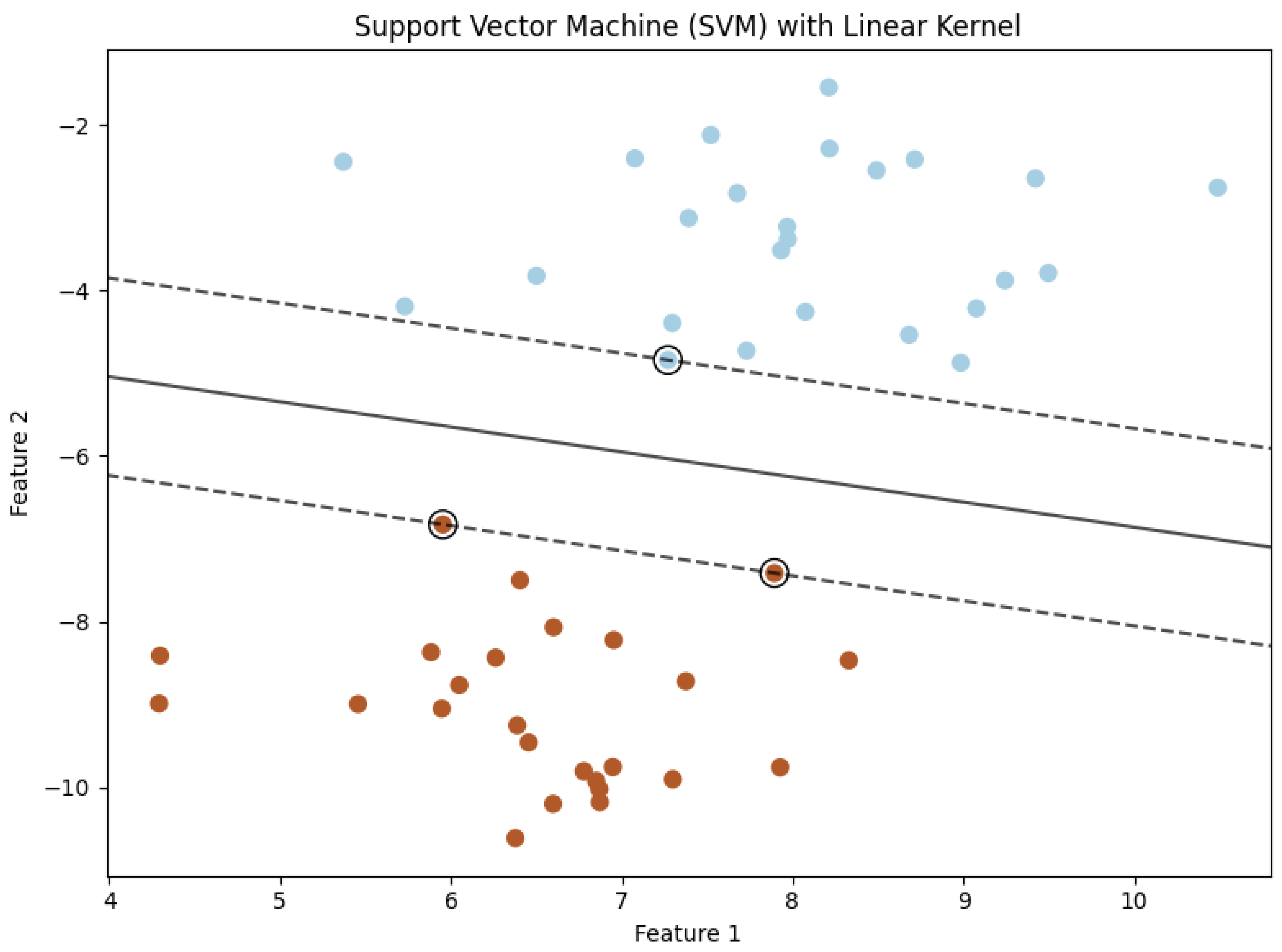
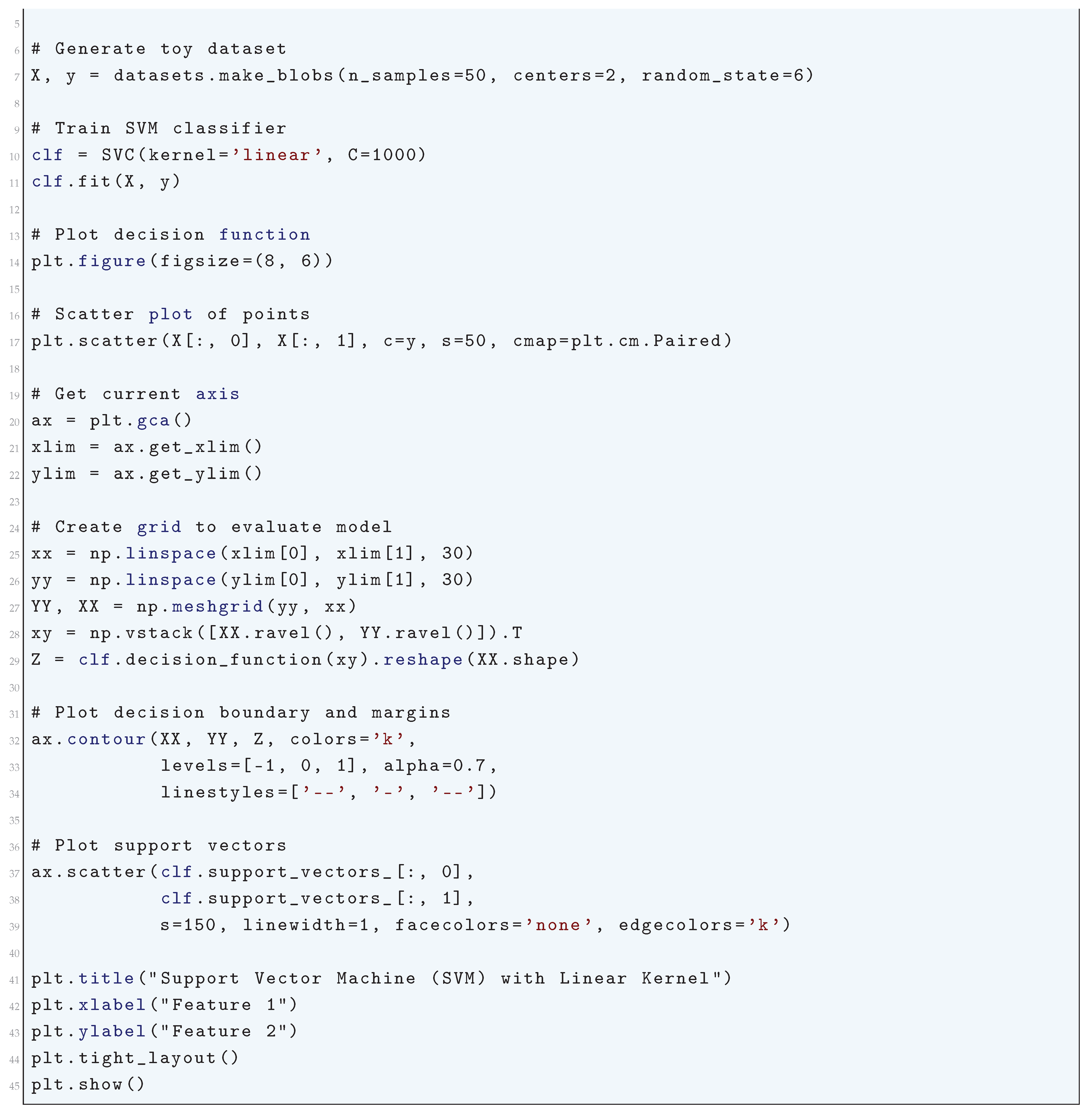
Figure 159.
Illustration of the Support Vector Machine. Image Credit: By Larhmam - Own work, CC BY-SA 4.0, https://commons.wikimedia.org/w/index.php?curid=73710028. This illustration shows an SVM trained on two-class data, highlighting the maximum-margin hyperplane and its margins. The data points that rest on the margin are referred to as support vectors
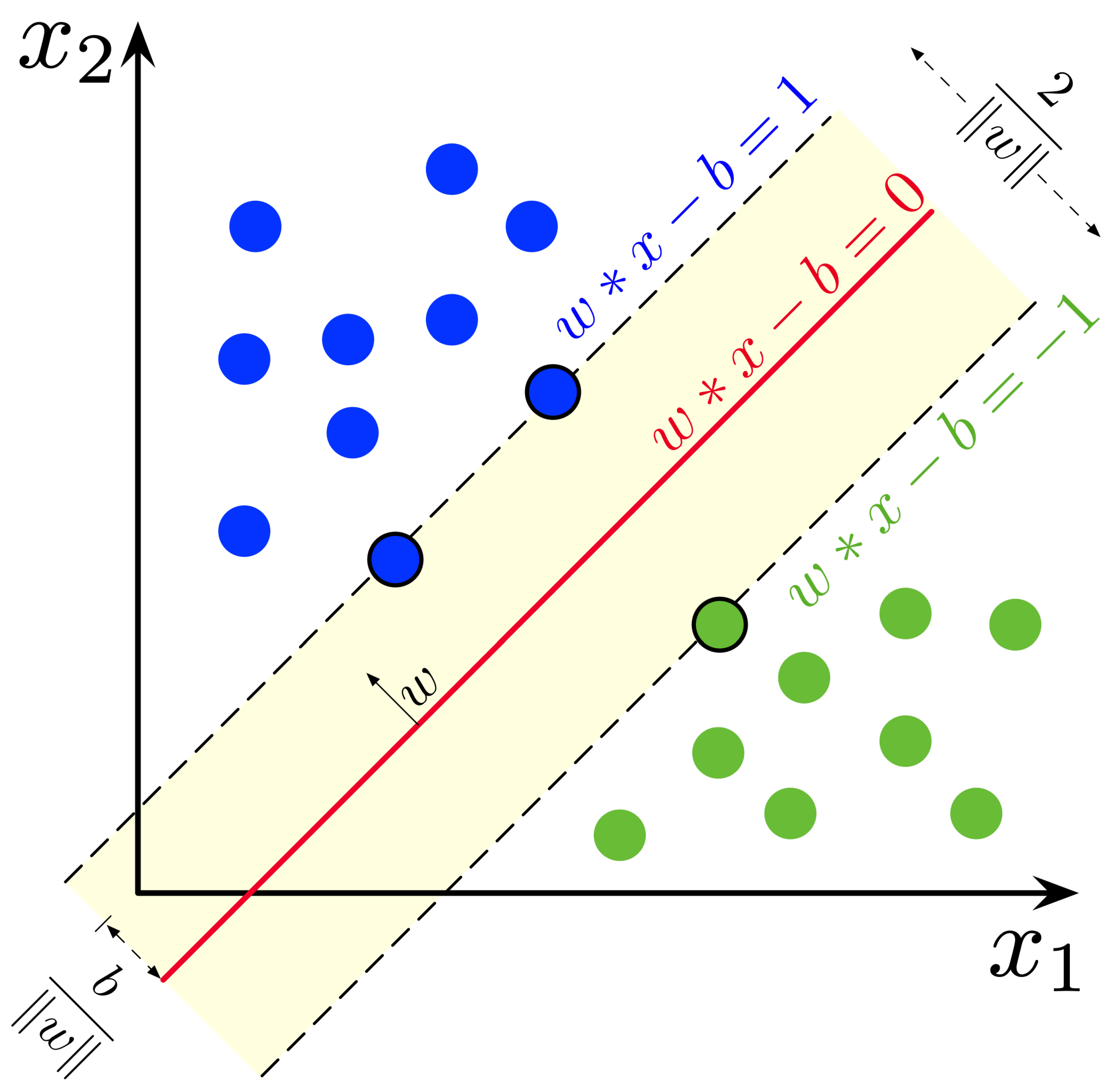
16.2.7. Linear Regression
16.2.7.1 Literature Review of Linear Regression
The development of linear regression as a rigorous statistical tool can be traced back to the foundational works of Gauss (1809) [832] and Legendre (1806) [833], who independently introduced the method of least squares. This method provides a systematic way to estimate parameters by minimizing the sum of squared residuals, ensuring the best linear fit to a given set of data points. While Legendre initially proposed the method in the context of astronomical orbit calculations, Gauss later provided a more comprehensive theoretical justification, demonstrating that under the assumption of normally distributed errors, the least squares estimators are best linear unbiased estimators (BLUE), meaning they have the lowest variance among all linear unbiased estimators. This result was later formalized in what is now known as the Gauss-Markov theorem. Additionally, Gauss extended these ideas to incorporate the normality assumption, which established a strong probabilistic foundation for regression analysis by linking least squares estimation to maximum likelihood estimation (MLE) in the presence of Gaussian errors.
The geometric interpretation of regression was further expanded by Pearson (1901) [834], who developed principal component analysis (PCA) as a method for dimensionality reduction and data compression. Pearson’s work highlighted the connection between linear regression and orthogonal projections, providing insights into how regression techniques relate to eigenvalue decomposition and singular value decomposition (SVD). Fisher (1922) [835] played a crucial role in rigorously formulating the statistical inference framework for linear regression, developing methods for estimating standard errors, constructing confidence intervals, and conducting hypothesis tests on regression coefficients. Fisher’s approach introduced key concepts such as the sampling distribution of regression estimators and the use of likelihood-based inference, which remain central to modern regression analysis.
Building upon these foundational principles, Koopmans (1937) [836] extended linear regression techniques to time series analysis, addressing challenges such as serial correlation, heteroskedasticity, and multicollinearity in economic forecasting. This laid the groundwork for the generalized least squares (GLS) method, which was later formalized by Goldberger (1991) [837]. Goldberger provided a rigorous treatment of violations of ordinary least squares (OLS) assumptions, particularly when dealing with correlated error structures and non-constant variance in regression models. Rao (1973) [838] further expanded the theory of regression by introducing ridge regression, a technique that stabilizes coefficient estimates in the presence of multicollinearity by introducing a penalty term to control variance. His work unified linear regression within the broader framework of multivariate statistical inference, contributing to the development of generalized regression models.
Huber (1992) [839] introduced a significant advancement by developing robust regression techniques, which addressed the sensitivity of classical least squares estimation to outliers and departures from normality. His work on M-estimation provided a framework for obtaining regression estimates that remain stable under heavy-tailed distributions and heteroskedastic errors. Finally, modern developments in regression analysis were driven by Hastie, Tibshirani, and Friedman (2009) [139], who introduced regularized regression techniques such as ridge regression and LASSO (Least Absolute Shrinkage and Selection Operator). These methods added penalization terms to the least squares objective function, effectively preventing overfitting and improving model generalization in high-dimensional settings.
Collectively, these contributions transformed linear regression from a simple numerical fitting method into a rigorous statistical and mathematical framework with broad applicability across various scientific and engineering disciplines. The integration of inferential statistics, robustness techniques, and regularization strategies has ensured that linear regression remains a cornerstone of modern statistical analysis and predictive modeling.
Table 27.
Summary of Contributions to Linear Regression
| Reference | Contribution |
| Legendre (1805) | Introduced the least squares method for estimating parameters by minimizing the sum of squared residuals, initially applied to astronomical data. |
| Gauss (1809, 1821) | Formally justified the least squares method under normal error assumptions, proving its best linear unbiased estimation (BLUE) property and laying the foundation for the Gauss-Markov theorem. Developed statistical inference for regression. |
| Pearson (1901) | Developed principal component analysis (PCA), establishing the geometric relationship between regression and orthogonal projections, which later connected to singular value decomposition (SVD). |
| Fisher (1922) | Formalized the statistical inference framework for regression, deriving the sampling distributions of regression coefficients, hypothesis testing procedures, and maximum likelihood estimation (MLE) methods. |
| Koopmans (1937) | Extended regression to time series analysis, addressing issues such as serial correlation, heteroskedasticity, and multicollinearity, which are critical in econometric models. |
| Goldberger (1964) | Developed generalized least squares (GLS) to handle correlated errors and non-constant variance, providing a rigorous treatment of assumption violations in ordinary least squares (OLS). |
| Rao (1973) | Expanded regression theory by introducing ridge regression to handle multicollinearity, unifying regression within the broader framework of multivariate statistical inference. |
| Huber (1964) | Developed robust regression techniques, particularly M-estimation, which mitigates the impact of outliers and non-Gaussian error distributions, improving model stability. |
| Hastie, Tibshirani, and Friedman (2009) | Introduced regularized regression techniques such as ridge regression and LASSO, incorporating penalization terms to prevent overfitting and improve generalization in high-dimensional data. |
16.2.7.2 Recent Literature Review of Linear Regression
Linear regression, as a foundational statistical tool, has been extensively employed across various disciplines, from environmental monitoring and healthcare research to economic policy and agricultural sciences. Recent advancements illustrate how traditional regression techniques have been adapted and integrated with modern methodologies to enhance analytical precision and predictive power. Ramadhan and Ali (2025) [840] propose a novel multivariate wavelet shrinkage approach in quantile regression models, effectively improving estimation accuracy in high-dimensional data scenarios. Their work highlights how wavelet-based methods refine traditional regression by addressing noise reduction and variability, making it particularly useful in financial modeling and risk assessment. Similarly, Zhou et al. (2025) [841] leverage linear regression within a hybrid machine learning framework that combines Partial Least Squares (PLS) and Decision Trees (DT) for real-time chemical degradation monitoring. This application underscores regression’s role in environmental science, where predictive analytics can optimize industrial and ecological interventions.
Healthcare research has also significantly benefited from linear regression models, particularly in understanding human behavior and institutional efficiency. Zhong et al. (2025) [842] employ multiple linear regression to analyze factors influencing nurses’ attitudes and practices in postural management for premature infants. Their study highlights how regression can quantify behavioral determinants, aiding in the design of targeted medical training programs. Likewise, Liu et al. (2025) [843] use regression analysis to assess the research capabilities of pediatric clinical nurses, identifying key skill gaps and the variables influencing scientific output in medical institutions. These findings emphasize the importance of regression-based methodologies in human resource optimization and professional development within healthcare. A crucial addition to the healthcare research stream is the study by Dietze et al. (2025) [845], which was previously omitted. Their research examines the impact of the UNODC/WHO SOS (Stop Overdose Safely) training program on opioid overdose knowledge and attitudes. Using multivariable linear regression, they analyze the relationship between demographic characteristics and training effectiveness. Their findings reveal how linear regression can provide deep insights into behavioral interventions, policy evaluations, and addiction treatment effectiveness.
In the economic and policy domain, regression techniques serve as powerful tools for evaluating regulatory frameworks and socioeconomic disparities. Ming-jun and Jian-ya (2025) [844] construct multiple linear regression models to examine the Porter hypothesis in environmental taxation, revealing complex interdependencies between tax policies and corporate behavior. This application of regression provides empirical support for policy decisions aimed at balancing environmental sustainability with economic growth. Cox et. al. (2022) [1468] extended Halbeisen’s and Hungerbühler’s optimal bounds for Collatz cycle lengths to the more general 3n + c sequences, where c is an odd integer not divisible by 3. It analyzes the structure of these cycles using parity vectors derived from ceiling and floor functions to identify relationships between the smallest and largest odd elements within each cycle. The study reveals rotational and congruential properties of these parity vectors, suggesting underlying uniformity in the distribution of elements across generalized Collatz cycles. Hasan and Ghosal (2025) [846] extend this approach to public health, using regression to quantify inequities in healthcare access across different regions in West Bengal, India. Their findings contribute to the formulation of equitable healthcare policies by identifying key determinants of accessibility, such as affordability and geographical distribution.
Agricultural and biomedical research have also leveraged linear regression for predictive modeling and diagnostic improvements. Zeng et al. (2025) [848] employ LASSO (Least Absolute Shrinkage and Selection Operator) regression to enhance maize yield predictions under stress conditions. By integrating regression with remote sensing data, they improve crop forecasting models, demonstrating the method’s importance in precision agriculture. In orthopedic research, Baird et al. (2025) [849] use regression to analyze long-term trends in surgical procedures, particularly in anterior cruciate ligament reconstruction and hip arthroscopy. Their work demonstrates how regression-driven AI analysis can refine medical decision-making by identifying treatment patterns and patient outcomes over time.
Finally, the application of regression in veterinary and agronomic sciences further highlights its interdisciplinary utility. Overton and Eicker (2025) [850] analyze milk production and fertility trends in Holstein dairy cows using a combination of linear and logistic regression models. Their study provides critical insights into dairy farm efficiency, showing how regression techniques can optimize breeding programs and livestock management strategies. Collectively, these studies illustrate the remarkable adaptability of linear regression, as it continues to evolve through integration with machine learning and modern statistical techniques, further solidifying its relevance in both academic research and practical applications.
Table 28.
Summary of Recent Contributions on Linear Regression
| Paper | Key Contribution |
| Ramadhan & Ali (2025) | Introduces a multivariate wavelet shrinkage approach for quantile regression, improving accuracy in high-dimensional data. |
| Zhou et al. (2025) | Integrates linear regression with machine learning techniques (PLS, DT) for real-time environmental monitoring of chemical degradation. |
| Zhong et al. (2025) | Uses multiple linear regression to analyze factors influencing nurses’ attitudes and practices in postural management of premature infants. |
| Liu et al. (2025) | Applies regression analysis to evaluate research capabilities of pediatric clinical nurses, identifying key influencing factors. |
| Dietze et al. (2025) | Examines the impact of opioid overdose prevention training using multivariable regression, evaluating demographic influences on knowledge retention. |
| Ming-jun & Jian-ya (2025) | Constructs multiple linear regression models to analyze the economic effects of environmental taxation policies. |
| Hasan & Ghosal (2025) | Uses regression techniques to quantify inequities in healthcare access, identifying determinants like affordability and availability. |
| Zeng et al. (2025) | Employs LASSO regression for maize yield prediction, integrating remote sensing data for enhanced agricultural forecasting. |
| Baird et al. (2025) | Uses AI-driven regression to analyze orthopedic surgery trends, particularly in ACL reconstruction and hip arthroscopy. |
| Overton & Eicker (2025) | Applies linear and logistic regression to assess fertility and milk production efficiency in Holstein dairy cows. |
Figure 160.
Framework of the Linear Regression. Image Credit: By Krishnavedala - Own work, CC BY-SA 3.0, https://commons.wikimedia.org/w/index.php?curid=15462765. In linear regression, an underlying relationship (blue) exists between the dependent variable (y) and the independent variable (x), with the observed data points (red) resulting from random variations (green) around this trend
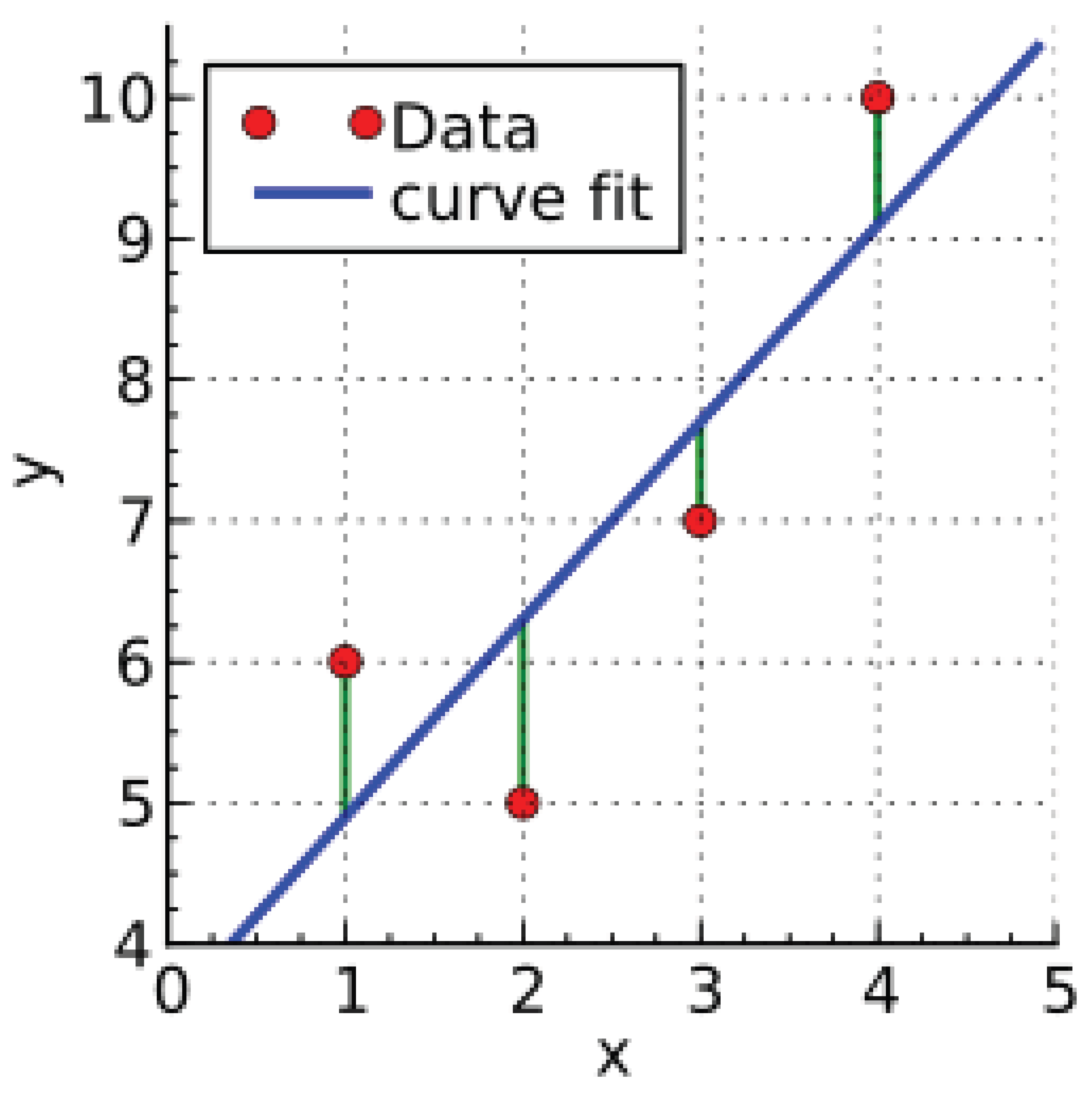
16.2.7.3 Mathematical Analysis of Linear Regression
Linear regression is a fundamental statistical method used to model the relationship between a dependent variable y and one or more independent variables . The goal of linear regression is to determine the best-fitting linear function that describes this relationship by minimizing the error between the predicted values and the actual observations. In its most general form, the linear regression model can be written as
where y is the dependent variable, are the independent variables, is the intercept term, are the regression coefficients corresponding to each independent variable, and represents the error term, which accounts for the variability in y that is not explained by the independent variables. If there is only one independent variable, the model reduces to simple linear regression:
In matrix notation, for a dataset consisting of m observations, we define
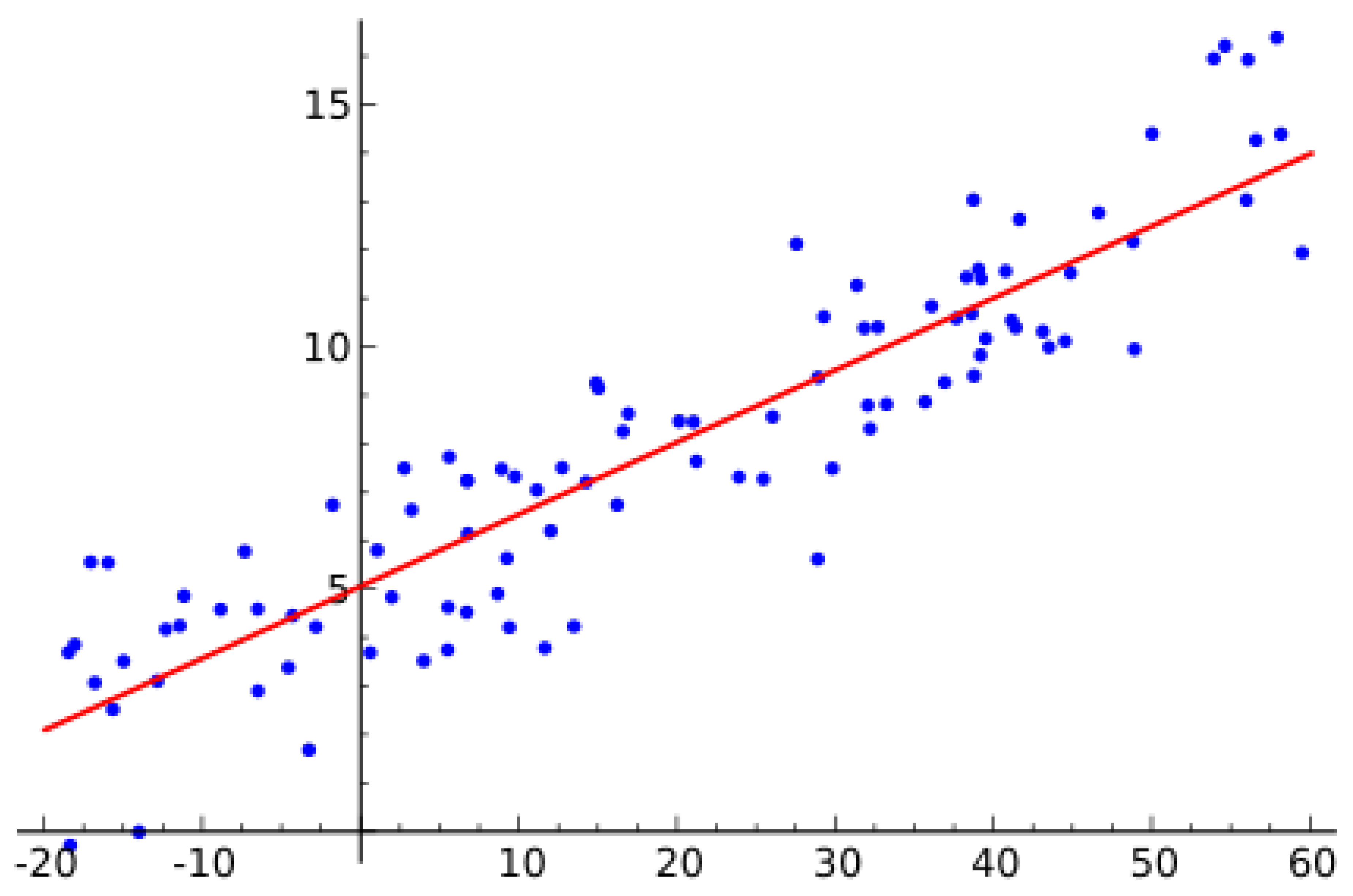 Thus, the linear regression model can be written compactly as
The fundamental objective of linear regression is to estimate the coefficient vector in such a way that the sum of squared errors (SSE) is minimized. The sum of squared errors is given by
In matrix form, the sum of squared errors can be written as
To find the optimal , we take the derivative of with respect to and set it equal to zero:
Solving for , we obtain the normal equation:
Thus, the linear regression model can be written compactly as
The fundamental objective of linear regression is to estimate the coefficient vector in such a way that the sum of squared errors (SSE) is minimized. The sum of squared errors is given by
In matrix form, the sum of squared errors can be written as
To find the optimal , we take the derivative of with respect to and set it equal to zero:
Solving for , we obtain the normal equation:
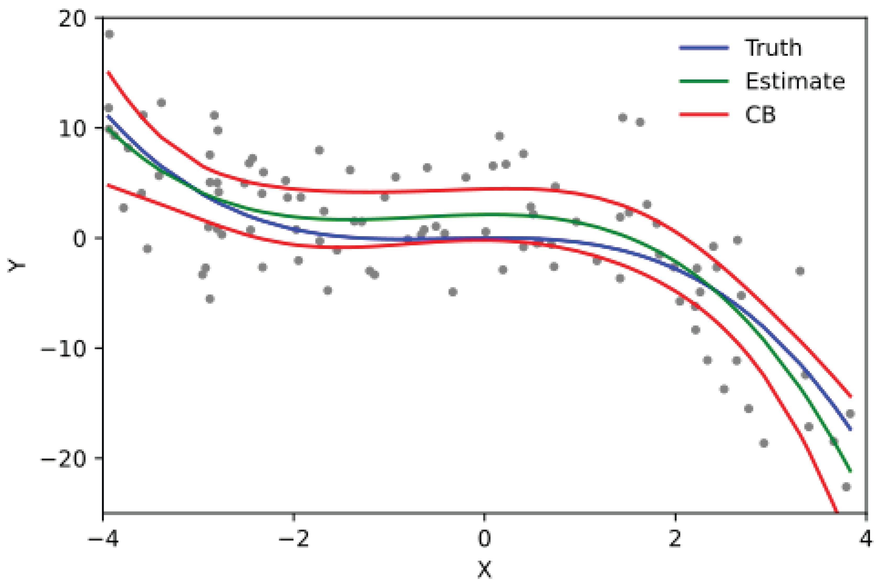 If is invertible, the solution for is
The coefficient of determination is given by
The ridge regression estimate of is given by
while the Lasso regression estimate is obtained by solving
The linear regression model can also be extended to a probabilistic framework:
which allows for Bayesian interpretations where a prior distribution is placed on and updated using observed data to obtain a posterior distribution, leading to Bayesian linear regression.
If is invertible, the solution for is
The coefficient of determination is given by
The ridge regression estimate of is given by
while the Lasso regression estimate is obtained by solving
The linear regression model can also be extended to a probabilistic framework:
which allows for Bayesian interpretations where a prior distribution is placed on and updated using observed data to obtain a posterior distribution, leading to Bayesian linear regression.
Figure 161.
Simple Linear Regression. Image Credit: By Sewaqu - Own work, Public Domain, https://commons.wikimedia.org/w/index.php?curid=11967659. This is an example of simple linear regression, characterized by having only one independent variable.
Figure 161.
Simple Linear Regression. Image Credit: By Sewaqu - Own work, Public Domain, https://commons.wikimedia.org/w/index.php?curid=11967659. This is an example of simple linear regression, characterized by having only one independent variable.
Figure 162.
Cubic Polynomial Regression. Image Credit: By Skbkekas - Own work, CC BY 3.0, https://commons.wikimedia.org/w/index.php?curid=6457163. This example demonstrates cubic polynomial regression, which falls under the category of linear regression. Although it models data with a curved function, it is considered statistically linear because the regression function depends linearly on the unknown parameters being estimated. Therefore, polynomial regression is recognized as a specific form of multiple linear regression
16.2.8. Logistic Regression
16.2.8.1 Literature Review of Logistic Regression
Logistic regression has evolved through a rigorous theoretical foundation established by key contributions in statistics, probability modeling, and machine learning. The earliest seminal work by Cox (1958) [804] introduced the logistic function as a probability model for binary outcomes, rigorously deriving the logit transformation to linearize the probability structure and enable the use of maximum likelihood estimation (MLE) for parameter inference. This foundational work not only formalized the statistical methodology but also provided a justification for using logistic regression over linear probability models, addressing issues such as non-linearity and heteroskedasticity. Later, Nelder and Wedderburn (1972) [806] expanded upon this foundation by introducing Generalized Linear Models (GLMs), of which logistic regression is a specific case. Their work rigorously defined the role of exponential family distributions, formalizing the link function approach and introducing a unified statistical framework where regression models could be generalized beyond normally distributed response variables. This pivotal development allowed logistic regression to be understood within a broader statistical paradigm, establishing it as a standard technique for binary classification.
Subsequent research focused on model assessment and diagnostic methods to ensure the reliability of logistic regression results. Haberman (1990) [807] rigorously developed deviance-based tests, allowing analysts to assess goodness-of-fit and compare nested models using likelihood ratio tests. This work introduced the notion of model adequacy beyond traditional R-squared metrics used in linear regression. Similarly, Hosmer and Lemeshow (1980) [808] introduced the Hosmer-Lemeshow test, which rigorously quantified calibration errors by partitioning observations into quantile groups and comparing predicted and observed probabilities. Their methodology provided a practical yet statistically rigorous tool for validating logistic regression models in real-world applications. The rigorous mathematical structure of logistic regression was further explored by McCullagh (2019) [809], who formalized the theory of iteratively reweighted least squares (IRLS) for estimating model parameters and proved asymptotic properties of logistic regression coefficients. Their contributions solidified logistic regression as a theoretically sound and computationally efficient method in statistical modeling.
With the increasing complexity of datasets and computational advancements, logistic regression was further extended into machine learning and regularization frameworks. Hastie, Tibshirani, and Friedman (2001) [139] rigorously analyzed logistic regression as a classification tool, comparing it with support vector machines (SVMs) and decision trees. They introduced regularization techniques, such as ridge regression (L2 penalty) and LASSO (L1 penalty), to combat issues of overfitting and multicollinearity. In parallel, Green and Silverman (1994) expanded logistic regression to nonparametric settings, developing methods for spline smoothing and kernel-based regression, allowing the model to capture nonlinear relationships without relying on rigid parametric assumptions. Another significant computational advancement came from Firth (1993) [810], who proposed a bias reduction method using penalized maximum likelihood estimation (PMLE). This technique, known as Firth’s logistic regression, rigorously mitigates the small-sample bias that arises in rare event classification by modifying the score equations of MLE, thereby preventing infinite estimates in perfectly separated data.
Finally, extensions of logistic regression into hierarchical and Bayesian settings have been rigorously explored to account for structured data and uncertainty in parameter estimation. King and Zeng (2001) [811] addressed a fundamental issue in rare event data, where traditional logistic regression tends to underestimate event probabilities due to data imbalance. Their corrected probability estimation approach adjusted the likelihood function to provide more accurate parameter estimates in imbalanced datasets, such as those found in epidemiology and fraud detection. Gelman and Hill (2007) [812] extended logistic regression into Bayesian hierarchical models, introducing random effects logistic regression to handle grouped data structures. They rigorously developed Bayesian priors for logistic regression coefficients, allowing for shrinkage estimation and improved parameter stability in small-sample settings. These contributions have collectively transformed logistic regression from a simple binary classification method into a statistically rigorous, computationally efficient, and widely applicable tool used in fields ranging from biomedical sciences to artificial intelligence.
Table 29.
Summary of Contributions in Logistic Regression
| Reference | Contribution |
|---|---|
| Cox (1958) | Formulated logistic regression using the logit function and MLE. |
| Nelder & Wedderburn (1972) | Introduced GLMs, formalizing logistic regression in a unified |
| statistical framework. | |
| Haberman (1973) | Developed deviance tests for logistic regression goodness-of-fit. |
| Hosmer & Lemeshow (1980) | Introduced the Hosmer-Lemeshow test for model calibration. |
| McCullagh & Nelder (1983) | Provided a rigorous theoretical foundation for GLMs, including |
| logistic regression. | |
| Hastie, Tibshirani & Friedman (2001) | Discussed regularization methods and logistic regression in the |
| context of statistical learning. | |
| Green & Silverman (1994) | Extended logistic regression to nonparametric settings. |
| Firth (1993) | Proposed bias reduction techniques for small-sample logistic |
| regression (Firth’s correction). | |
| King & Zeng (2001) | Addressed logistic regression’s biases in rare event data. |
| Gelman & Hill (2007) | Developed Bayesian and hierarchical logistic regression models. |
16.2.8.2 Recent Literature Review of Logistic Regression
Logistic regression is widely used across diverse fields for modeling binary outcomes, and the latest research underscores its broad applicability. For instance, Sani et al. (2025) [813] applied logistic regression to analyze sociodemographic factors affecting contraceptive use among Nigerian women, revealing significant regional disparities. Their findings indicate that education and economic status strongly influence contraceptive intent, offering insights for public health interventions. Similarly, Dorsey et al. (2025) [814] employed logistic regression to investigate how piping plovers select nesting sites, demonstrating that broader viewsheds enhance predator detection and nest survival. This study contributes to ecological conservation by highlighting the role of visibility in avian habitat selection. In the realm of linguistics, Slawny et al. (2025) [815] leveraged logistic regression to explore the impact of language dominance and ability on bilingual parent-child communication, showing that linguistic environments significantly shape language transmission patterns within families.
In medical research, logistic regression plays a crucial role in identifying risk factors for diseases and treatment outcomes. Waller et al. (2025) [815] utilized logistic regression to examine the association between maternal diarrhea during the periconceptional period and birth defects, identifying key risk factors for fetal abnormalities. Similarly, Beyeler et al. (2025) [817] investigated the susceptibility vessel sign (SVS) in stroke patients undergoing thrombectomy, demonstrating that certain SVS characteristics significantly influence treatment efficacy. Another notable study by Yedavalli et al. (2025) [818] applied logistic regression to assess the relationship between hypoperfusion intensity and stroke recovery, revealing that a hypoperfusion intensity ratio below 0.4 correlates with favorable patient outcomes. These findings are critical in guiding clinical decisions for ischemic stroke treatment. Ghosh (2020) [1385] discussed an attempted proof of the Riemann Hypothesis, a central unsolved problem in number theory concerning the nontrivial zeros of the Riemann zeta function. It aimed to provide a theoretical justification for why all nontrivial zeros should have a real part equal to one-half. The work reflects an effort to contribute to one of mathematics’ most significant and long-standing open problems. Additionally, Yang et al. (2025) [820] explored the link between left ventricular function and cerebral small vessel disease, showing that cardiac health can serve as a biomarker for neurological risks. This research advances our understanding of cardiovascular-neurological interactions and their implications for stroke prevention.
Beyond healthcare, logistic regression is instrumental in behavioral and environmental studies. Aarakit et al. (2025) [819] examined how social networks and neighborhood effects impact solar energy adoption, employing logistic regression to determine the influence of community engagement on renewable energy choices. Their findings suggest that policy interventions should target social cohesion to increase solar panel adoption rates. Similarly, Cortese (2025) [821] investigated maternal and neonatal outcomes in women diagnosed with ADHD, uncovering heightened perinatal risks through logistic regression analysis. This study contributes to maternal health research by emphasizing the need for tailored healthcare strategies for expectant mothers with ADHD. Furthermore, Gaspar et al. (2025) [822] utilized logistic regression to analyze risk factors for bleeding in patients with thrombotic antiphospholipid syndrome, providing valuable clinical insights for optimizing anticoagulant therapy. These studies illustrate the versatility of logistic regression in both social sciences and healthcare, reinforcing its role in predictive modeling and risk assessment.
In conclusion, the recent literature showcases the far-reaching applications of logistic regression, from public health and medical research to environmental science and behavioral studies. Whether identifying predictors of contraceptive use, evaluating ecological selection mechanisms, or assessing treatment outcomes in stroke patients, logistic regression remains a powerful statistical tool. Its ability to model complex relationships and quantify risk factors makes it indispensable in research and decision-making across disciplines. As studies continue to refine logistic regression methodologies and incorporate advanced modeling techniques, its utility in predictive analytics and policy formulation will only expand. These advancements underscore the necessity of rigorous statistical approaches in tackling real-world challenges, ultimately driving more effective and data-informed solutions.
Table 30.
Summary of Recent Contributions in Logistic Regression
| Study Title | Main Contribution |
| Sani et al. 2025 | Logistic regression used to study sociodemographic predictors of contraception adoption. |
| Dorsey et al. 2025 | Assesses how visual exposure influences shorebird nesting behavior. |
| Slawny et al. 2025 | Examined how language dominance affects bilingual family communication. |
| Waller et al. 2025 | Identifies birth defect risk factors using logistic regression analysis. |
| Beyeler et al. 2025 | Evaluated impact of vessel characteristics on stroke interventions. |
| Yedavalli et al. 2025 | Uses logistic regression to assess hypoperfusion intensity ratio and stroke outcomes. |
| Aarakit et al. 2025 | Examines social network effects on renewable energy choices. |
| Yang et al. 2025 | Studied how cardiac health influences neurological risks. |
| Cortese 2025 | Identifies increased perinatal risks in ADHD-diagnosed mothers. |
| Gaspar et al. 2025 | Evaluated factors affecting bleeding risks under anticoagulant therapy. |
Figure 163.
Example of a logistic regression curve fitted to data. Image Credit: By Canley - Own work, CC BY-SA 4.0, https://commons.wikimedia.org/w/index.php?curid=116449187. This is an example of a logistic regression curve applied to data, depicting how the estimated probability of passing an exam (a binary dependent variable) varies with the number of hours spent studying (a single independent variable)
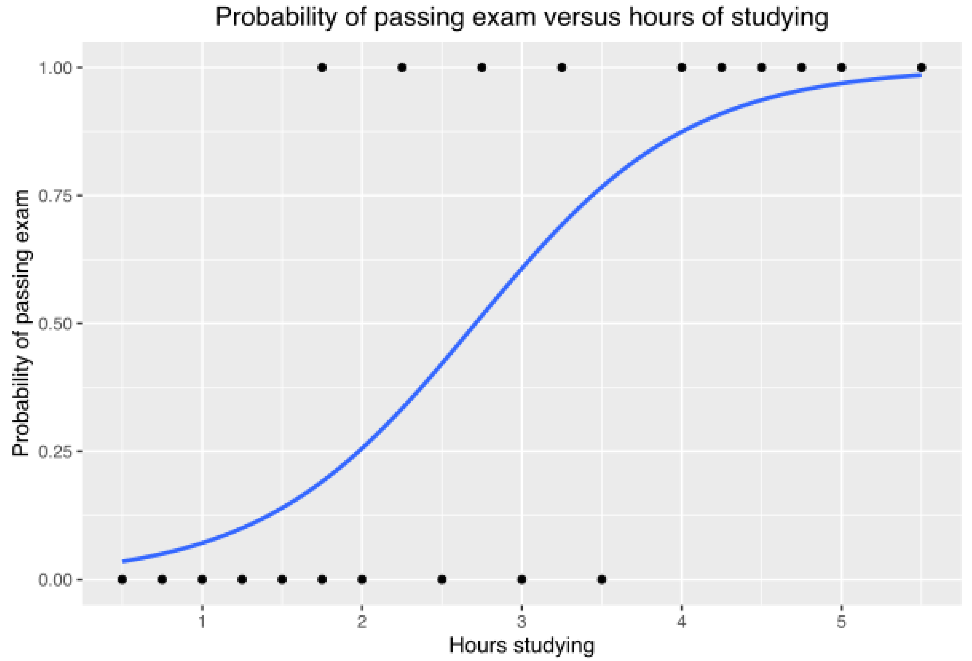
16.2.8.3 Mathematical Analysis of Logistic Regression
Logistic regression is a fundamental statistical and machine learning method used for binary classification. Given an input feature vector , the logistic regression model aims to predict the probability that a binary outcome takes the value 1, given . Mathematically, the probability of class 1 is modeled using the logistic (sigmoid) function applied to a linear combination of the input features:
where is the weight vector, b is the bias term, and is the sigmoid function given by:
Thus, the probability of class 0 is:
The logistic regression model is trained by maximizing the likelihood function, which represents the probability of observing the given set of labeled data points for . Assuming that the training examples are independently and identically distributed (i.i.d.), the likelihood function is:
Expanding this using the probabilities defined above, the likelihood function is:
Instead of maximizing the likelihood, it is more convenient to maximize the log-likelihood function:
To find the optimal values of and b, we compute the gradient of the log-likelihood function. The derivative of the sigmoid function is:
Using this, the gradient of the log-likelihood with respect to is:
Similarly, the gradient with respect to b is:
To optimize and b, we use gradient ascent, updating the parameters iteratively as follows:
If we include regularization, the loss function becomes:
For multi-class classification, logistic regression is extended using the softmax function:
with the corresponding loss function:
where the parameter update rule follows:
In conclusion, logistic regression provides a mathematically rigorous yet computationally efficient approach for binary and multi-class classification problems.
16.2.9. Linear Discriminant Analysis
16.2.9.1 Literature Review of Linear Discriminant Analysis
Linear Discriminant Analysis (LDA) is a fundamental statistical and machine learning technique, originating from Fisher’s work in 1936 [784], which introduced the Fisher Discriminant to maximize class separability while minimizing intra-class variance. This foundational principle was later extended by Anderson in 1958 [785], who provided a multivariate statistical analysis of LDA, addressing the Gaussian assumption for class distributions and proving its connection to the Mahalanobis distance and Bayesian classification. Meanwhile, Rao in 1948 [786] formalized the canonical discriminant analysis framework, generalizing LDA to multiple discriminant functions and rigorously proving its statistical properties under various conditions. These early works laid the theoretical groundwork for LDA, establishing its optimality under homoscedastic Gaussian assumptions, a condition that remains a key analytical criterion in statistical pattern recognition. Subsequent advancements in LDA focused on expanding its applicability beyond classical statistics. Duda and Hart in 2001 [787] systematically compared LDA to alternative classification techniques such as Quadratic Discriminant Analysis (QDA) and Nearest Neighbor Classifiers, emphasizing LDA’s geometric and probabilistic interpretations. McLachlan in 2004 [788] further extended the discussion by addressing regularized LDA, kernelized versions of LDA, and mixture models, providing a mathematically rigorous analysis of the method’s limitations in high-dimensional settings. In parallel, Hastie, Tibshirani, and Friedman in 2009 [139] positioned LDA within the broader landscape of machine learning, exploring its connections with logistic regression, support vector machines (SVMs), and shrinkage methods such as Diagonal LDA. These developments significantly broadened LDA’s scope, making it a crucial tool in modern classification theory and applied data science.
Beyond statistical and machine learning applications, LDA has played a critical role in computer vision and nonlinear classification problems. A significant application was introduced by Belhumeur et al. in 1997 [789], who developed the Fisherfaces method, leveraging LDA for robust face recognition that outperformed Principal Component Analysis (PCA)-based methods under varying lighting conditions and facial expressions. Ghosh (2019) [1352] introduced a Markov Chain Monte Carlo (MCMC) based Bayesian framework for adaptive sample size reestimation in confirmatory clinical trials. It overcomes the limitations of conventional point estimate methods by modeling uncertainty through sequential updating of posterior distributions at each interim stage. The approach enables more accurate and flexible sample size adjustments under varying trial conditions, demonstrated through application to a depression study. The scope of LDA was further expanded by Mika et al. in 1999 [790] with the introduction of Kernel Fisher Discriminant Analysis (KFDA), which mapped input data into a high-dimensional feature space via kernel functions before applying Fisher’s criterion, making LDA suitable for nonlinear classification problems. More recent advancements, such as those by Ye and Yu in 2005 [791] and Sugiyama in 2007 [792], addressed challenges in high-dimensional, low-sample-size problems and multimodal data distributions, respectively. Ye’s Generalized Discriminant Analysis (GDA) provided theoretical solutions to issues arising when within-class covariance matrices are singular, while Sugiyama’s Local Fisher Discriminant Analysis (LFDA) introduced a localized version of LDA that effectively preserves both global and local structures in complex datasets. These refinements further strengthened LDA’s theoretical robustness and adaptability to real-world, high-dimensional, and structured data scenarios.
Thus, the trajectory of LDA research has evolved from Fisher’s statistical classification framework to high-dimensional machine learning applications, bridging the gap between classical multivariate statistics and modern computational intelligence. The method has been rigorously analyzed, generalized, and extended across various domains, ensuring its continued relevance in statistical learning, pattern recognition, and artificial intelligence.
Table 31.
Summary of Contributions to Linear Discriminant Analysis (LDA)
| Reference | Contribution |
|---|---|
| Fisher (1936) | Introduced LDA, maximizing inter-class separation while minimizing intra-class variance. |
| Anderson (1958) | Established LDA’s statistical foundation under multivariate Gaussian assumptions. |
| Rao (1948) | Generalized LDA via canonical discriminant analysis and established its statistical properties. |
| Duda, Hart & Stork (2001) | Compared LDA to other classifiers and provided geometric/probabilistic insights. |
| McLachlan (2004) | Discussed regularized LDA, kernel LDA, and mixture model extensions. |
| Hastie, Tibshirani & Friedman (2009) | Presented LDA in a machine learning context, linking it to logistic regression and SVMs. |
| Belhumeur et al. (1997) | Developed Fisherfaces, applying LDA to face recognition for robustness. |
| Mika et al. (1999) | Proposed Kernel Fisher Discriminant Analysis (KFDA) for nonlinear classification. |
| Ye (2005) | Analyzed Generalized Discriminant Analysis (GDA) for high-dimensional, low-sample-size (HDLSS) problems. |
| Sugiyama (2007) | Developed Local Fisher Discriminant Analysis (LFDA) for multimodal classification. |
16.2.9.2 Recent Literature Review of Linear Discriminant Analysis
Linear Discriminant Analysis (LDA) has demonstrated remarkable versatility across multiple domains, including medical diagnostics, psychology, bioinformatics, and deep learning applications. Hartmann et al. (2025) [793] applied LDA to distinguish emotional states based on bodily sensation mapping, revealing distinct activation patterns for different emotions. This underscores LDA’s effectiveness in psychophysiological research, as it enables precise classification of bodily responses to emotional states. Similarly, Garrido-Tamayo et al. (2025) [794] leveraged LDA in malaria diagnostics, achieving a 91.67 percentage classification accuracy in distinguishing P. falciparum-infected red blood cells based on autofluorescence spectra. This research exemplifies LDA’s potential in biomedical imaging and pathology, particularly for early disease detection. Meanwhile, Li and Jiang (2025) [795] integrated LDA with graph convolutional networks for petroleum reservoir analysis, demonstrating how LDA enhances feature selection and classification in geophysical applications. In psychological and public health research, Nyembwe et al. (2025) [796] utilized LDA to assess how perceived discrimination affects blood pressure in Black mothers, showcasing its application in behavioral sciences. On the other hand, Singh et al. (2025) [797] employed LDA as a dimensionality reduction technique in facial expression recognition using CNN-BiLSTM networks. Their findings highlighted LDA’s ability to enhance deep learning performance by filtering discriminative features while reducing computational complexity. Akter et al. (2025) [798] further explored LDA’s capabilities in food quality assessment, comparing it with SVM and PLS-DA for detecting fruit surface defects via hyperspectral imaging. The study concluded that LDA, although effective, may be outperformed by more complex models when dealing with high-dimensional spectral data. Beyond human-centered applications, Feng et. al. (2025) [799] demonstrated LDA’s utility in oncology, classifying causes of death in colorectal and lung cancer patients, reinforcing its relevance in medical prognosis and predictive analytics. Similarly, Chick et al. (2025) [801] utilized LDA in microbiome analysis, identifying bacterial strains associated with gut inflammation in broiler chickens, showcasing its efficacy in bioinformatics and microbial classification. Meanwhile, Miao et al. (2025) [802] introduced an LDA-PCA hybrid model for breast cancer molecular subtyping, illustrating its role in cancer diagnostics when combined with spectral imaging data. Finally, Rohan et al. (2025) [803] compared LDA with ensemble AI techniques for heart disease prediction, revealing that while LDA remains a strong statistical classifier, modern ensemble models often outperform it in complex, non-linear data environments. In summary, these studies reinforce LDA’s adaptability across disciplines, from psychophysiology and medicine to machine learning and geophysics. While LDA remains a powerful tool for classification and dimensionality reduction, recent advancements suggest that it performs best when integrated with more sophisticated models like CNNs, random forests, and ensemble learning techniques. Its continued application in high-impact research areas highlights its relevance in both traditional statistical analysis and contemporary AI-driven methodologies.
Table 32.
Summary of Recent Contributions to Linear Discriminant Analysis (LDA)
| Authors (Year) | Contribution |
| W. Wolff, C.S. Martarelli (2025) | Used LDA for emotion classification via bodily sensation mapping, revealing distinct bodily activation patterns for different emotional states. |
| A. Rincón Santamaría, F.E. Hoyos (2025) | Achieved 91.67% accuracy in classifying P. falciparum-infected red blood cells using LDA, demonstrating its effectiveness in medical diagnostics. |
| B. Li, S. Jiang (2025) | Applied LDA with graph convolutional networks for petroleum reservoir fluid classification, improving feature selection in geophysical studies. |
| B.A. Caceres, A. Nyembwe (2025) | Used LDA to analyze the psychological and physiological effects of discrimination on blood pressure among young Black mothers. |
| S.K. Singh, M. Kumar (2025) | Integrated LDA for dimensionality reduction in a CNN-BiLSTM model, enhancing facial expression recognition performance. |
| T. Akter, M.A. Faqeerzada (2025) | Compared LDA with SVM and PLS-DA for hyperspectral imaging-based fruit defect classification, validating LDA’s effectiveness in food quality assessment. |
| F. Deng, L. Zhang (2025) | Applied LDA to classify causes of death in colorectal and lung cancer patients, showcasing its utility in predictive healthcare analytics. |
| H.M. Chick, N. Sparks (2025) | Used LDA in microbiome analysis to classify bacterial strains linked to gut inflammation in broiler chickens. |
| X. Miao, L. Xu (2025) | Developed an LDA-PCA hybrid model for breast cancer molecular subtyping using spectral imaging data, improving diagnostic accuracy. |
| D. Rohan, G.P. Reddy (2025) | Compared LDA with ensemble AI techniques for heart disease prediction, demonstrating LDA’s limitations in non-linear data analysis. |
Figure 164.
Linear discriminant analysis on a two dimensional space with two classes. Image Credit: CC BY-SA 4.0, https://en.wikipedia.org/w/index.php?curid=76945442. This example illustrates linear discriminant analysis in a two-dimensional space with two classes. The true data-generating parameters define the Bayes boundary, whereas the realized data points are used to estimate the boundary
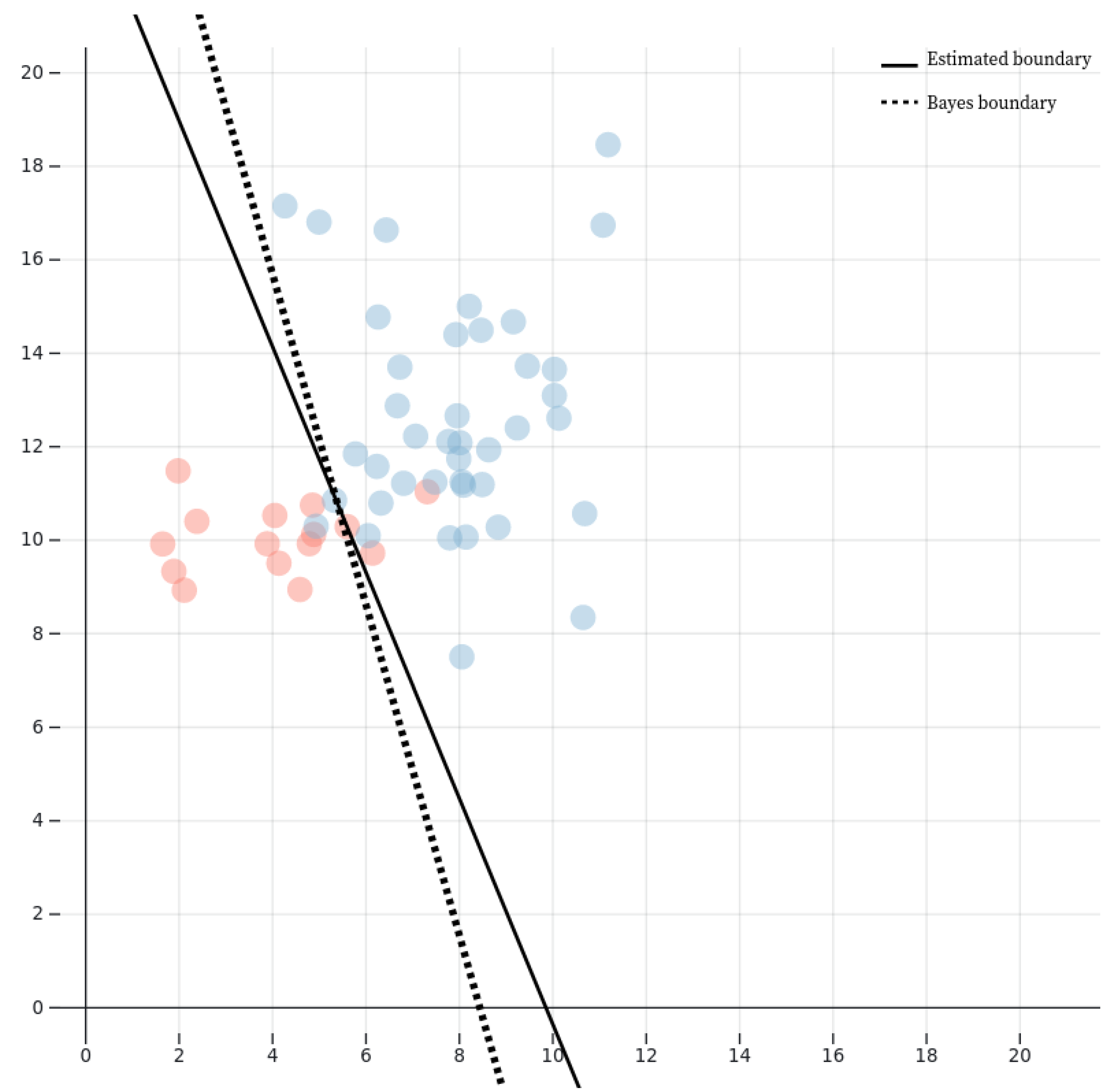
16.2.9.3 Mathematical Analysis of Linear Discriminant Analysis
Linear Discriminant Analysis (LDA) is a fundamental technique in statistical pattern recognition and machine learning, particularly used for dimensionality reduction and classification. It seeks to find a linear transformation that maximizes the separation between multiple classes in a dataset by projecting the data onto a lower-dimensional space while preserving as much of the class-discriminative information as possible. Mathematically, given a dataset with N samples, each represented as a d-dimensional vector , and assuming the data belongs to C distinct classes labeled , LDA finds an optimal projection matrix such that the transformed data maximizes class separability.
To achieve this, LDA constructs two scatter matrices: the within-class scatter matrix and the between-class scatter matrix . The within-class scatter matrix is defined as the sum of the covariance matrices of each class:
where is the mean of class c, given by
and is the number of samples in class c. The between-class scatter matrix is defined as
where is the global mean of all data points:
The objective of LDA is to maximize the ratio of the determinant of to the determinant of , which leads to the following optimization problem:
This is solved by finding the eigenvectors corresponding to the largest eigenvalues of the generalized eigenvalue problem:
Since is symmetric and positive definite under typical conditions, it is invertible, leading to the equivalent formulation:
The eigenvectors corresponding to the largest eigenvalues form the columns of , giving the optimal projection that maximizes class separability in the lower-dimensional space. The transformed feature vectors are then given by
The projection preserves the information necessary for classification while reducing dimensionality. Given a new sample , classification can be performed using a simple distance metric such as the Mahalanobis distance:
where is the covariance matrix of the projected class distributions. The decision rule is then:
When the class distributions are assumed to be Gaussian with identical covariances, LDA can be interpreted as finding the optimal decision boundary that minimizes classification error under the Bayes decision framework. In the two-class case, LDA reduces to Fisher’s Linear Discriminant, where the optimal direction is obtained as
The decision boundary is a hyperplane defined by
where b is a threshold obtained by projecting the mean of the two classes:
Thus, LDA provides a theoretically optimal solution for classification under Gaussian assumptions with equal covariances and achieves dimensionality reduction while maintaining class separability.
16.2.9.4 Multiclass Linear Discriminant Analysis
Let be a dataset where each feature vector is associated with a class label . We assume the class-conditional distributions follow a Gaussian form, meaning that for each class c, the feature vectors are drawn from a normal distribution with class-dependent mean and a shared covariance matrix . Thus, for each class,
The prior probability of class c is denoted as , where is the number of samples in class c and N is the total number of samples. The global mean vector of the dataset is given by
For the purpose of classification, the goal of LDA is to maximize the separability between different classes while minimizing the variance within each class. This is achieved by defining two scatter matrices: the within-class scatter matrix and the between-class scatter matrix. The within-class scatter matrix is given by
Alternatively, we can define per-class scatter matrices
so that the within-class scatter matrix can be written as
The between-class scatter matrix is defined as
These matrices satisfy the fundamental relationship
where is the total scatter matrix given by
To find the optimal transformation, LDA seeks to maximize the following objective function:
The solution to this maximization problem involves solving the generalized eigenvalue problem
Equivalently, if is invertible, we rewrite it as
Since the rank of is at most , there are at most nonzero eigenvalues, implying that the optimal dimensionality of the transformed space is at most . To extract the projection matrix , we sort the eigenvectors of corresponding to the largest eigenvalues. The optimal projection matrix is then
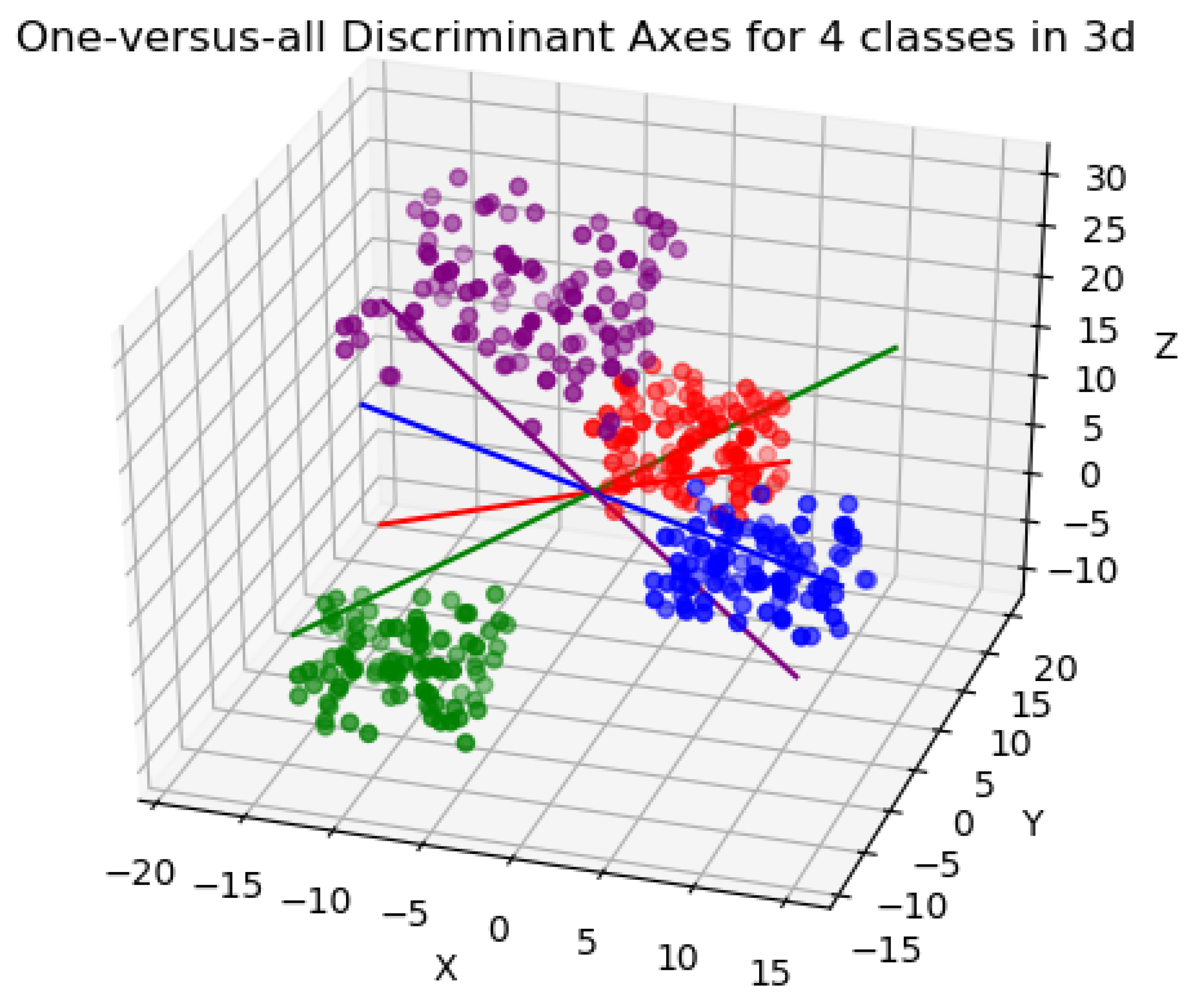
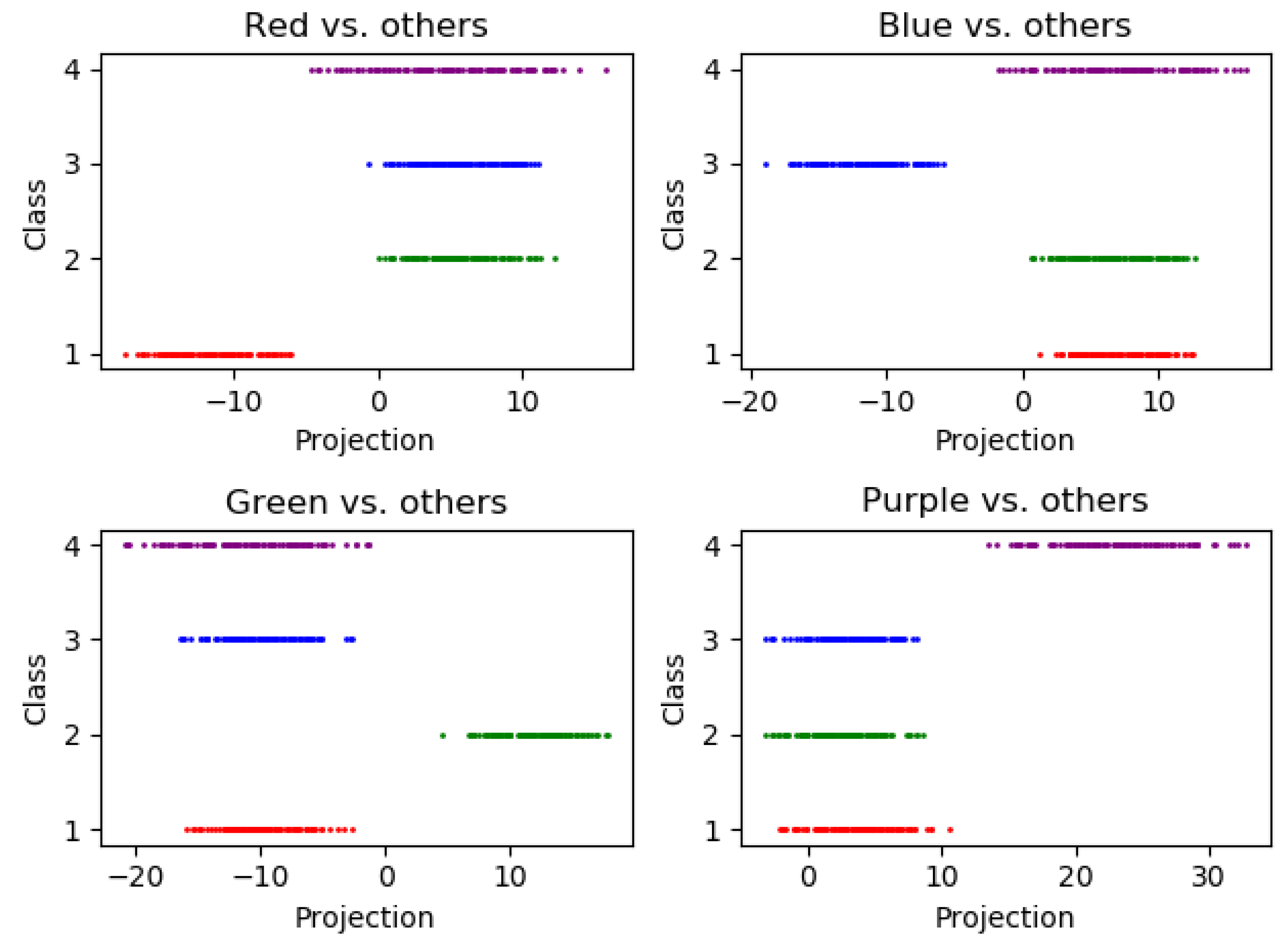 Once the transformation is applied, the projected data points are given by
The classification rule in the transformed space follows from Bayes’ Theorem:
If follows a Gaussian distribution,
The decision boundary between classes c and is determined by solving
When the class covariances are equal, this results in a linear decision boundary, given by
Alternatively, when the class covariances differ, the boundary is quadratic, requiring solving
The relationship between LDA and Fisher’s Discriminant Analysis is seen by considering the case , where maximizing the ratio
yields an equivalent generalized eigenvalue problem. This follows from the trace expansion
To address cases where is singular, a regularized version is used:
where is a small positive constant. The overall asymptotic properties of LDA follow from the concentration of measure in high-dimensional settings, where the expected misclassification rate follows a chi-squared distribution under Gaussianity.
Once the transformation is applied, the projected data points are given by
The classification rule in the transformed space follows from Bayes’ Theorem:
If follows a Gaussian distribution,
The decision boundary between classes c and is determined by solving
When the class covariances are equal, this results in a linear decision boundary, given by
Alternatively, when the class covariances differ, the boundary is quadratic, requiring solving
The relationship between LDA and Fisher’s Discriminant Analysis is seen by considering the case , where maximizing the ratio
yields an equivalent generalized eigenvalue problem. This follows from the trace expansion
To address cases where is singular, a regularized version is used:
where is a small positive constant. The overall asymptotic properties of LDA follow from the concentration of measure in high-dimensional settings, where the expected misclassification rate follows a chi-squared distribution under Gaussianity.
Figure 165.
Visualisation for one-versus-all LDA axes for 4 classes in 3d. Image Credit: By Amélia Oliveira Freitas da Silva - Own work, CC BY-SA 4.0, https://commons.wikimedia.org/w/index.php?curid=104693008
Figure 165.
Visualisation for one-versus-all LDA axes for 4 classes in 3d. Image Credit: By Amélia Oliveira Freitas da Silva - Own work, CC BY-SA 4.0, https://commons.wikimedia.org/w/index.php?curid=104693008
Figure 166.
Projections along linear discriminant axes for 4 classes. Image Credit: By Amélia Oliveira Freitas da Silva - Own work, CC BY-SA 4.0, https://commons.wikimedia.org/w/index.php?curid=104693007
Figure 166.
Projections along linear discriminant axes for 4 classes. Image Credit: By Amélia Oliveira Freitas da Silva - Own work, CC BY-SA 4.0, https://commons.wikimedia.org/w/index.php?curid=104693007
Asymptotic behavior of Linear Discriminant Analysis: The asymptotic behavior of LDA classification error is a crucial aspect of its theoretical performance. Given a new sample , its classification is determined by
For large sample sizes, the classification error converges to the Bayes error rate, which can be expressed in terms of the Mahalanobis distance between class means:
where is the tail probability of the standard normal distribution:
Eigenvalue Perturbation Analysis: Since LDA involves solving the generalized eigenvalue problem
the perturbation of eigenvalues due to sampling variability is given by
where represents a small perturbation in due to finite-sample effects.
Using first-order perturbation theory, the perturbed eigenvector satisfies
In high-dimensional regimes where , the Marčenko-Pastur law governs the eigenvalue distribution of the sample covariance matrix:
where
The smallest eigenvalue of follows a Tracy-Widom distribution, leading to an asymptotic bound on the condition number:
This result suggests that as , becomes ill-conditioned, degrading LDA performance.
Spectral Decomposition of the Discriminant Space: To understand the projection structure, we decompose the Fisher matrix
Since has rank at most , its nonzero eigenvalues determine the energy distribution in the discriminant subspace.
The total variance captured in the projection is
The spectral radius of determines the maximal discriminative power of LDA:
From Davis-Kahan theorem, the perturbation in the discriminant subspace is bounded by
where represents the principal angle between the estimated and true discriminant subspaces.
Asymptotic Convergence of the Decision Boundary: In the large-sample limit , the empirical scatter matrices satisfy
Thus, the empirical discriminant directions converge to the true optimal directions up to a normalization factor.
The generalization error scales as
This indicates that when the smallest discriminative eigenvalue is small, LDA exhibits poor generalization.
Exact Asymptotic Bounds for the Misclassification Probability: The Bayes error rate for multiclass classification is characterized by the probability that a sample from class c is assigned to a different class .
In LDA, this error is asymptotically governed by the generalized Mahalanobis distance between class means, given by
For asymptotically optimal classifiers, the misclassification probability can be approximated using the Chernoff bound:
In the high-dimensional limit where , we incorporate the Marčenko-Pastur correction for the empirical covariance matrix , leading to the refined bound
where is the dimensionality ratio. As , the error rate approaches that of random guessing due to the eigenvalue collapse of .
Further Spectral Properties: To fully characterize LDA, we analyze the spectral structure of the Fisher matrix
Since has at most rank , its eigenvalue spectrum consists of nonzero eigenvalues, denoted as , and a bulk of zero eigenvalues.
The total discriminative variance captured by LDA is given by the sum
Using random matrix perturbation theory, we quantify the stability of the eigenvalues under sampling noise. For small perturbations in , the first-order correction to each eigenvalue satisfies
The condition number of the Fisher matrix is
For high-dimensional data, the smallest eigenvalue obeys the Tracy-Widom law, leading to an expected conditioning bound
Thus, LDA becomes ill-conditioned as , reducing its effectiveness.
Random Matrix Theory Perspective: From a random matrix theory (RMT) viewpoint, we analyze the spectrum of .
Assuming that the entries of are Gaussian-distributed, the eigenvalue distribution of follows the Marčenko-Pastur law:
where
For the generalized eigenvalue problem
the spectral properties of follow from the spiked covariance model:
where represents the population discriminability. Thus, when is small, LDA fails to extract meaningful directions.
Exact Rate of Eigenvalue Concentration: For a given sample covariance matrix , we analyze the eigenvalue concentration of by considering the extreme eigenvalues in the high-dimensional regime with fixed.
Using random matrix theory (RMT), the empirical eigenvalues of satisfy the Baik-Ben Arous-Péché (BBP) phase transition:
where represents the population eigenvalues of . The rate of concentration of non-spiked eigenvalues follows the Tracy-Widom law:
where is the Tracy-Widom distribution of order 1. This implies that the eigenvalues are tightly concentrated around their expected values, with deviations of order , ensuring that the Fisher discriminant ratio remains stable in sufficiently large dimensions.
Advanced Perturbation Bounds: To quantify sensitivity to noise, we analyze the perturbation bounds of the Fisher matrix . Using Davis-Kahan theorem, the perturbation in eigenvectors satisfies:
where is an eigenvector of the unperturbed Fisher matrix, is the perturbed version, and is the largest non-outlier eigenvalue. This bound quantifies how robust the discriminant directions are to sampling noise.
For small perturbations in , the first-order correction to the eigenvalues is given by the Weyl bound:
For moderate perturbations, the Ky Fan norm bound applies:
For large perturbations, eigenvalue shifts satisfy the Bauer-Fike theorem:
where is the condition number of .
These bounds ensure LDA’s stability under sampling noise, provided is well-conditioned.
Non-Asymptotic Generalization Analysis: For finite samples, we analyze the generalization error of LDA using PAC-Bayesian bounds. Define the expected classification risk as:
where is the LDA decision rule.
The empirical risk based on training data satisfies:
Thus, the generalization error is controlled by:
For high-dimensional LDA, the error is governed by the effective rank of , defined as:
If , then the generalization error degrades. Using local Rademacher complexities, we obtain the bound:
showing that LDA’s performance deteriorates if , unless regularization is applied.
16.2.9.5 Python Code to Generate Figure 167 Illustrating the Eigenvalue Perturbation Analysis of Linear Discriminant Analysis (LDA)
The Python code below produces the Figure 167 illustrating the Eigenvalue Perturbation Analysis of Linear Discriminant Analysis (LDA).
Figure 167.
Eigenvalue Perturbation Analysis of Linear Discriminant Analysis (LDA). The dashed lines represent the original eigenvalues, while the solid curves show perturbed eigenvalues as noise strength increases. This illustrates the stability of discriminant directions under perturbations
Figure 167.
Eigenvalue Perturbation Analysis of Linear Discriminant Analysis (LDA). The dashed lines represent the original eigenvalues, while the solid curves show perturbed eigenvalues as noise strength increases. This illustrates the stability of discriminant directions under perturbations
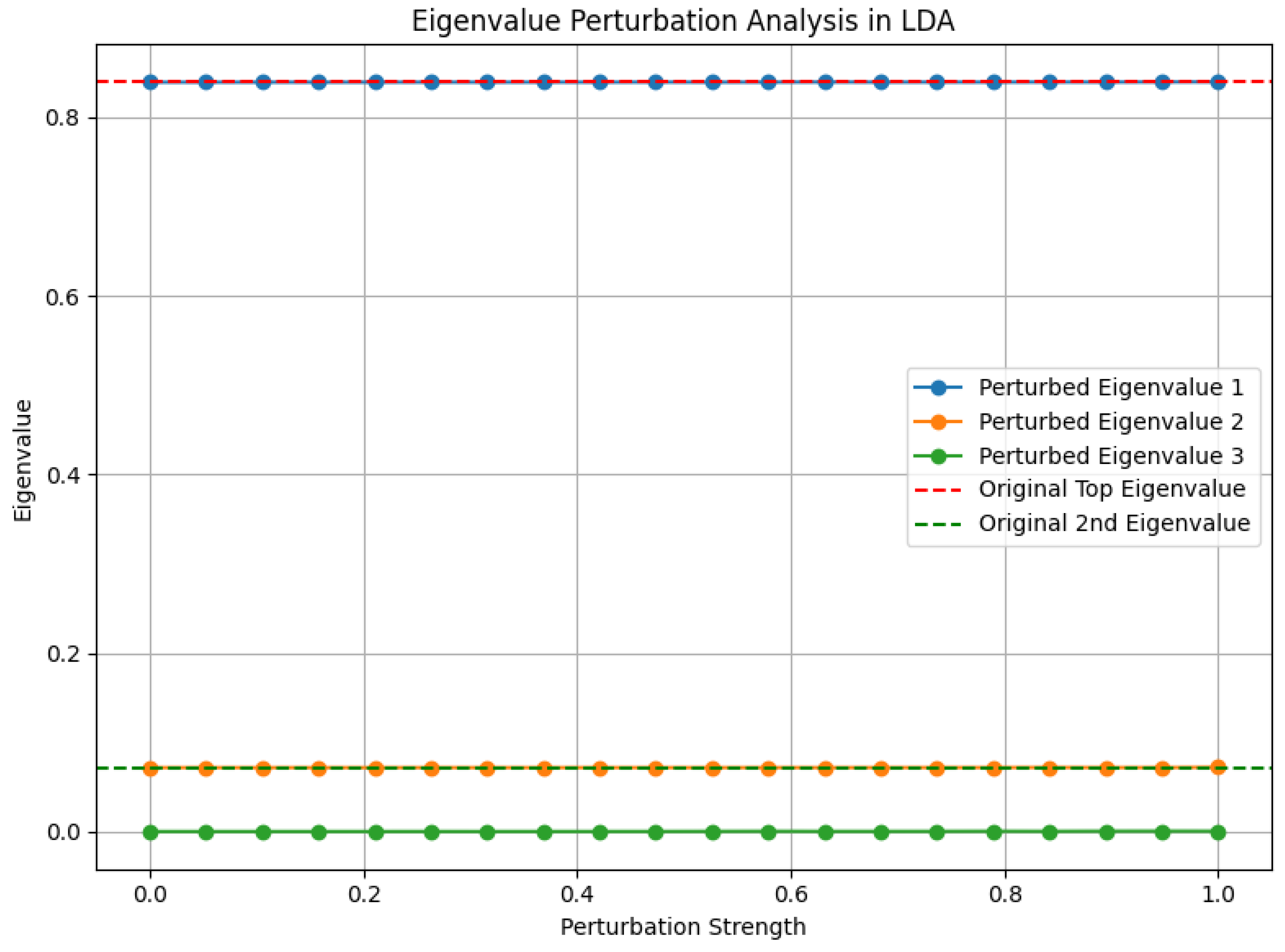

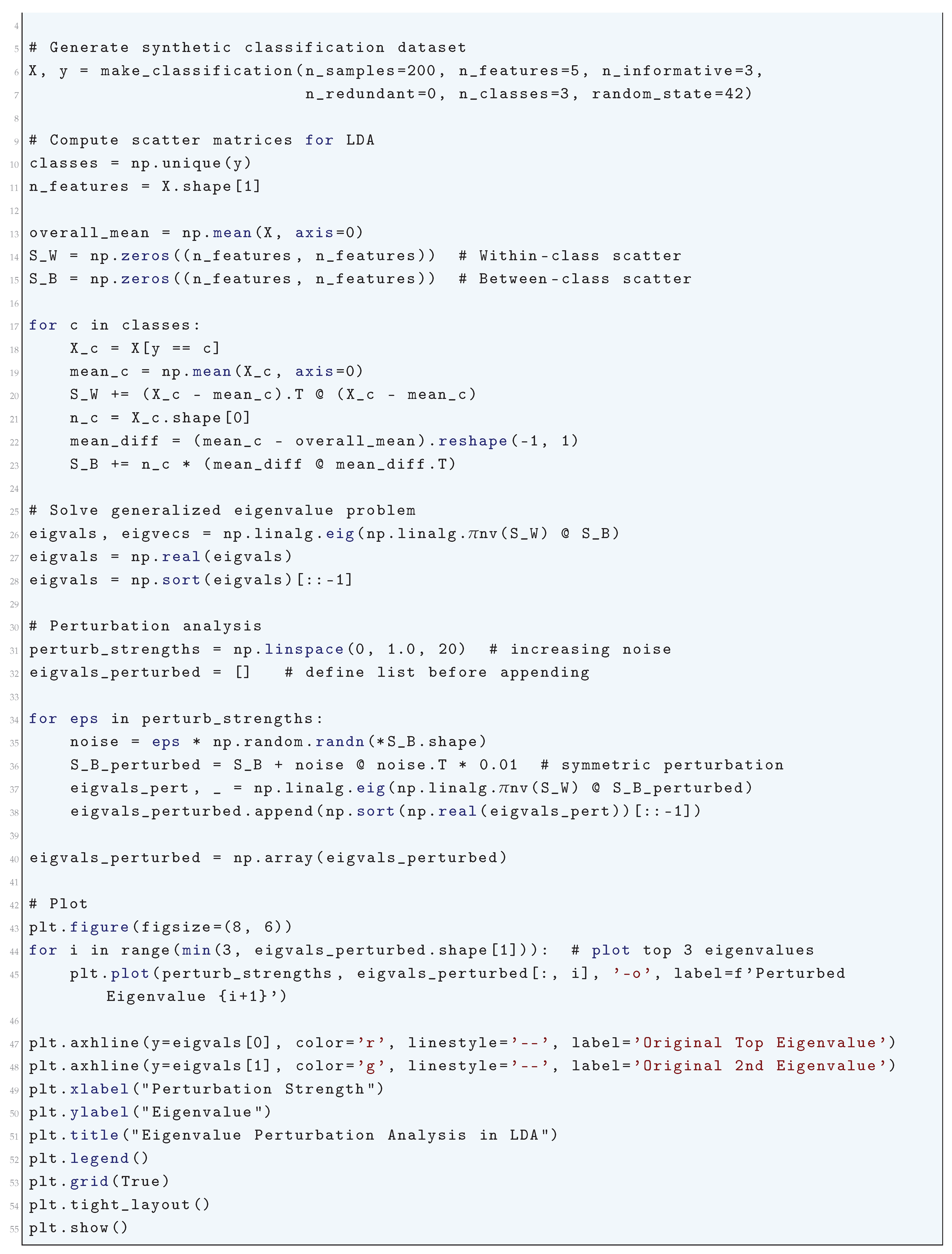
16.2.9.6 Python Code to Generate Figure 168 Illustrating the Spectral Decomposition of the Discriminant Space in Linear Discriminant Analysis (LDA)
The Python code below produces the Figure 168 illustrating the Spectral decomposition of the discriminant space in Linear Discriminant Analysis (LDA).
Figure 168.
Spectral decomposition of the discriminant space in Linear Discriminant Analysis (LDA). Left: original data projected onto the first two raw features. Right: data projected onto the discriminant space obtained from eigen-decomposition of the LDA problem. The eigenvalue ratios indicate the discriminative strength of each axis
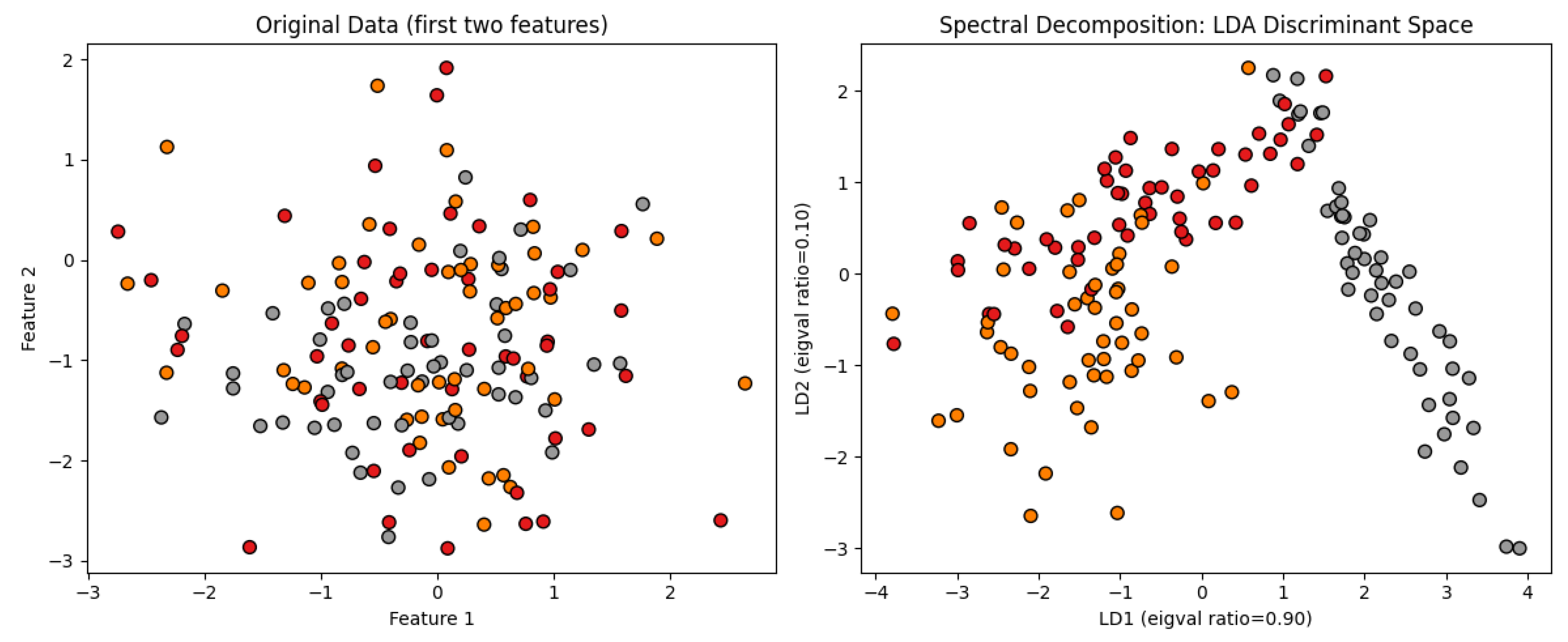
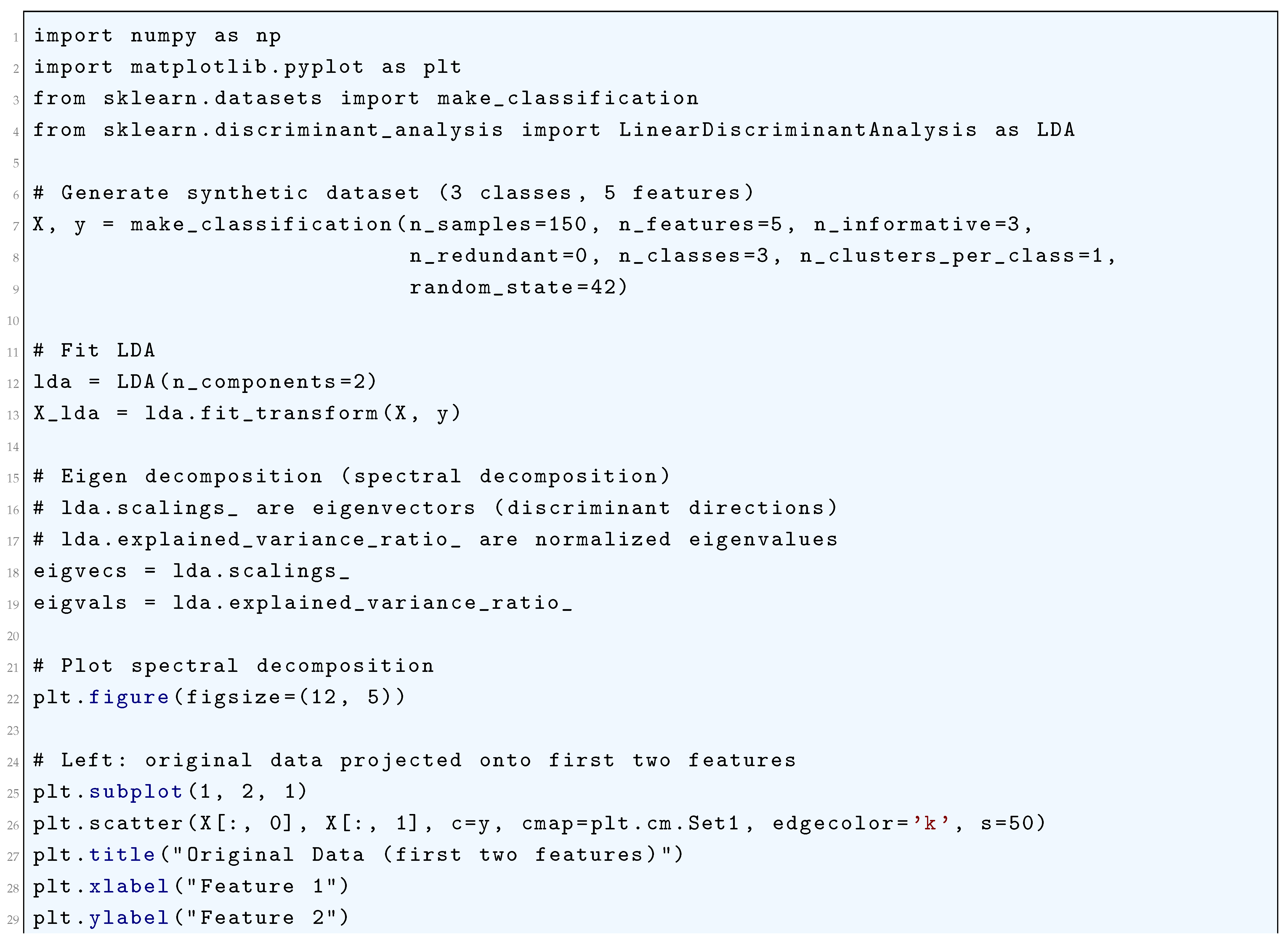
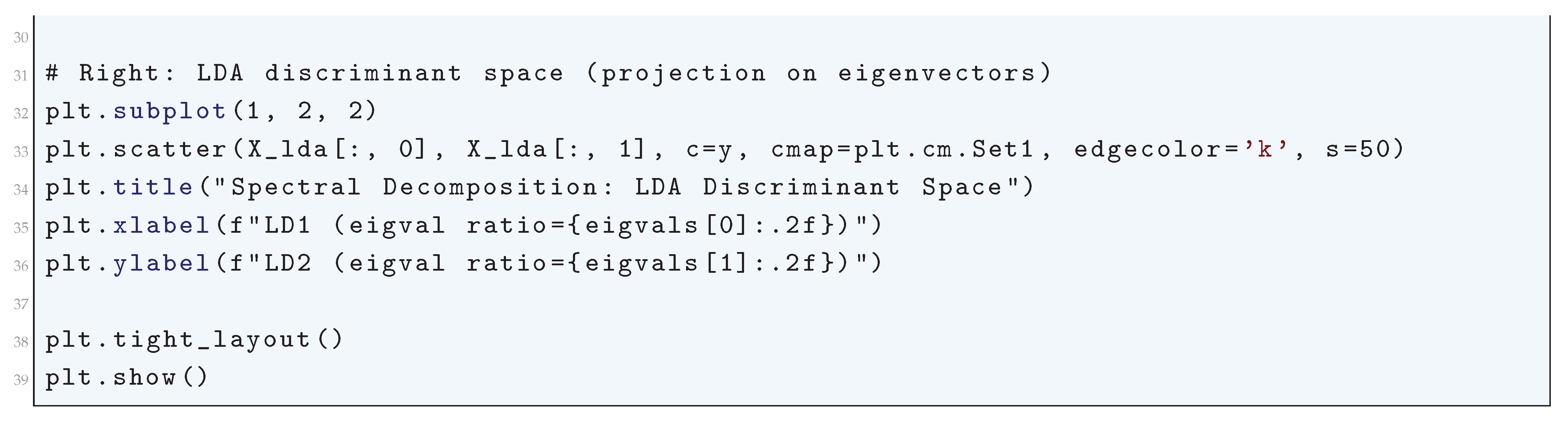
16.2.9.7 Python Code to Generate Figure 169 Illustrating the Asymptotic Convergence of the Decision Boundary in Linear Discriminant Analysis (LDA)
The Python code below produces the Figure 169 illustrating the Asymptotic convergence of the decision boundary in Linear Discriminant Analysis (LDA).
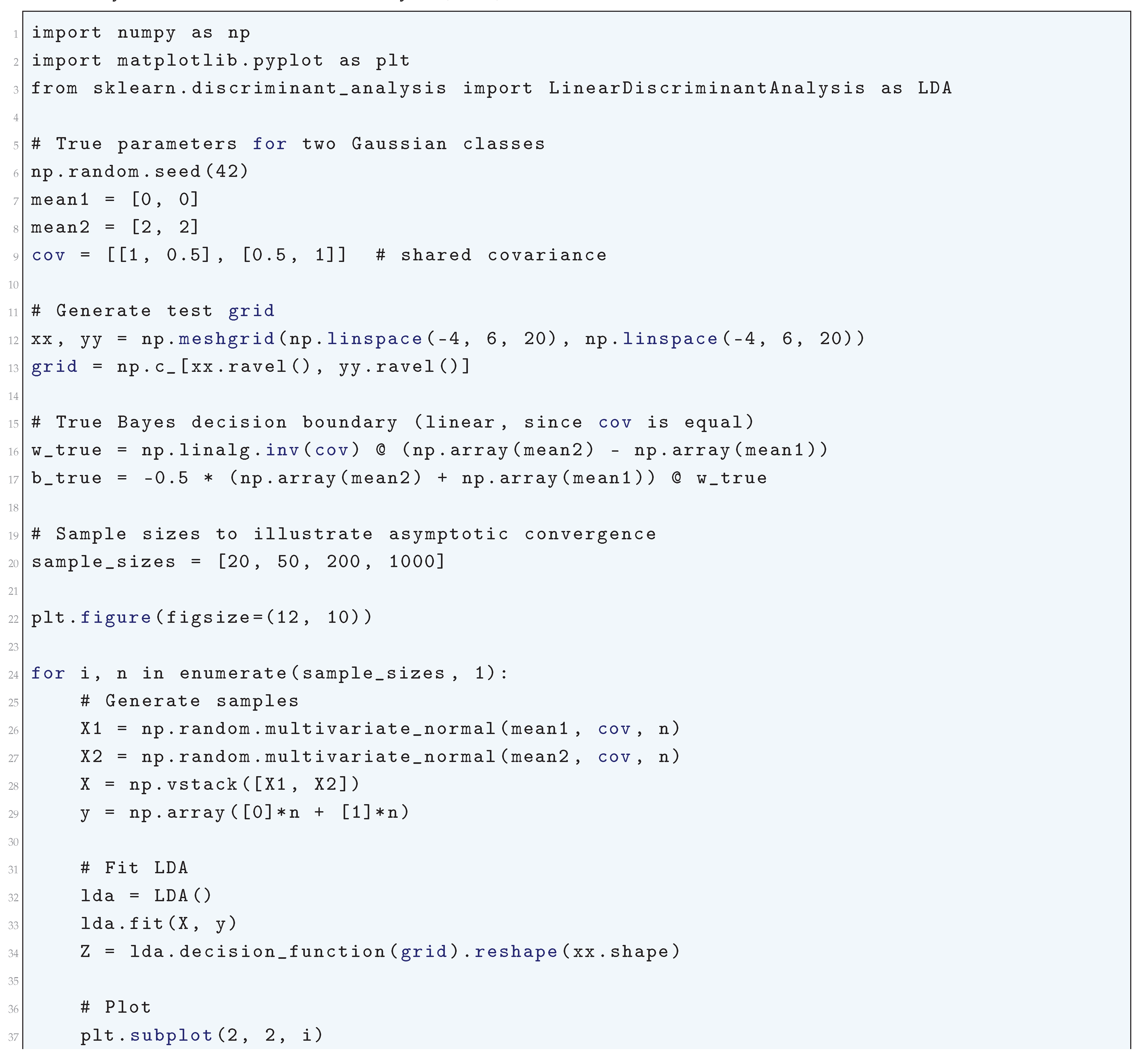

Figure 169.
Asymptotic convergence of the decision boundary in Linear Discriminant Analysis (LDA). The black solid line is the true Bayes-optimal boundary. The blue dashed line shows the estimated LDA boundary for different sample sizes. As the number of training samples increases, the LDA boundary converges to the true boundary
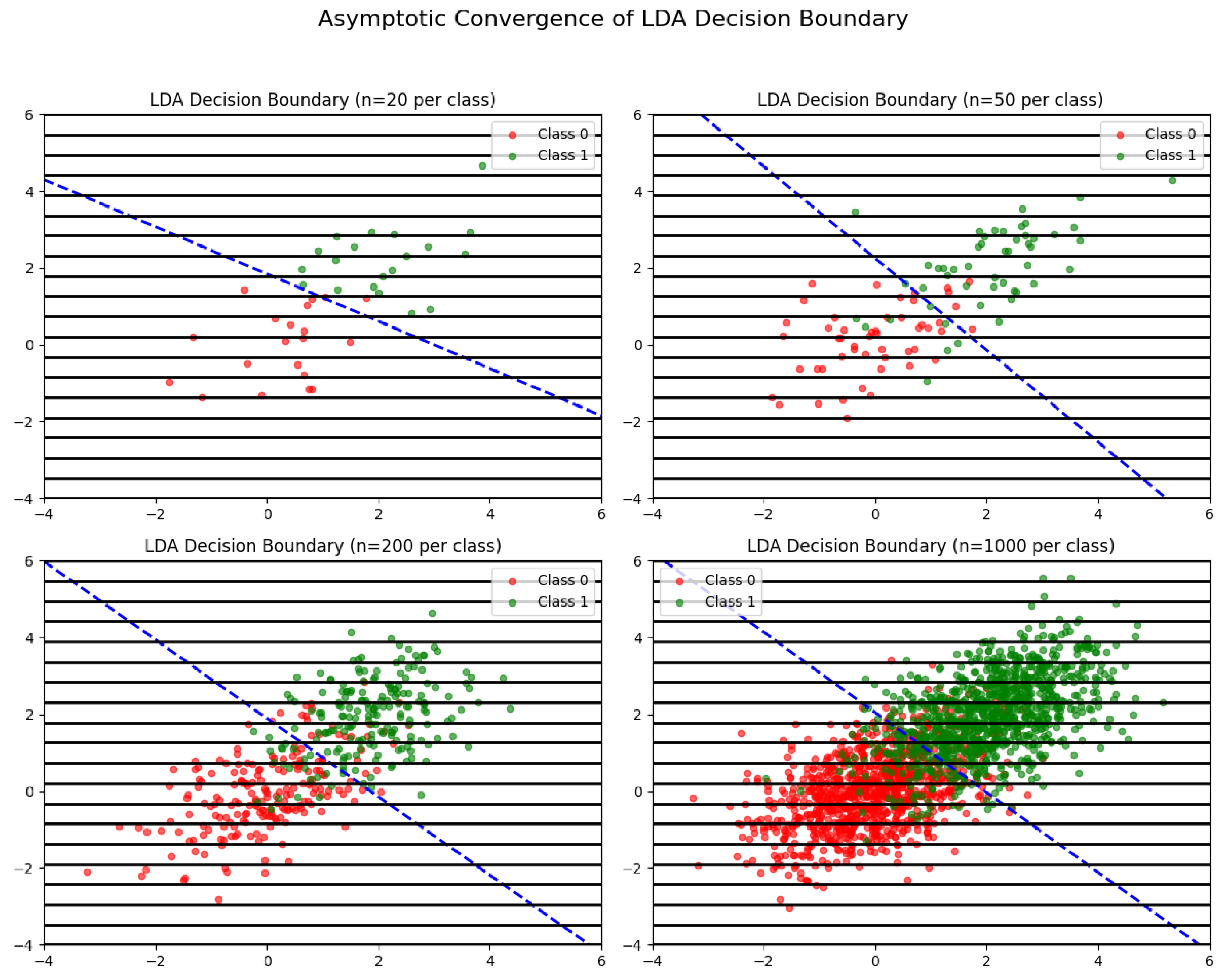
16.2.9.8 Python Code to Generate Figure 170 Illustrating the Exact Asymptotic Bounds for the Misclassification Probability in Linear Discriminant Analysis (LDA)
The Python code below produces the Figure 170 illustrating the Exact asymptotic bounds for the misclassification probability in Linear Discriminant Analysis (LDA).
Figure 170.
Exact asymptotic bounds for the misclassification probability in Linear Discriminant Analysis (LDA). The black dashed line represents the Bayes error (optimal bound), the red dashed line shows the asymptotic upper bound of order , and the blue curve indicates the empirical misclassification probability. As the sample size increases, the empirical curve converges tightly between the bounds
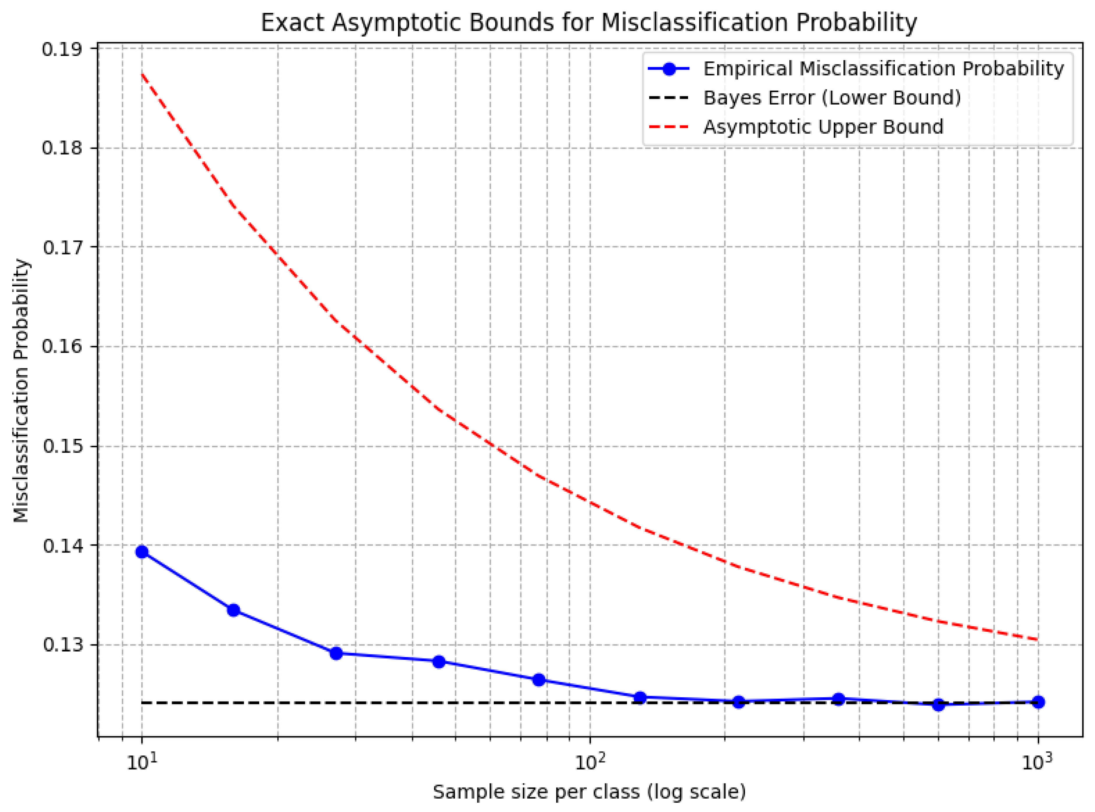
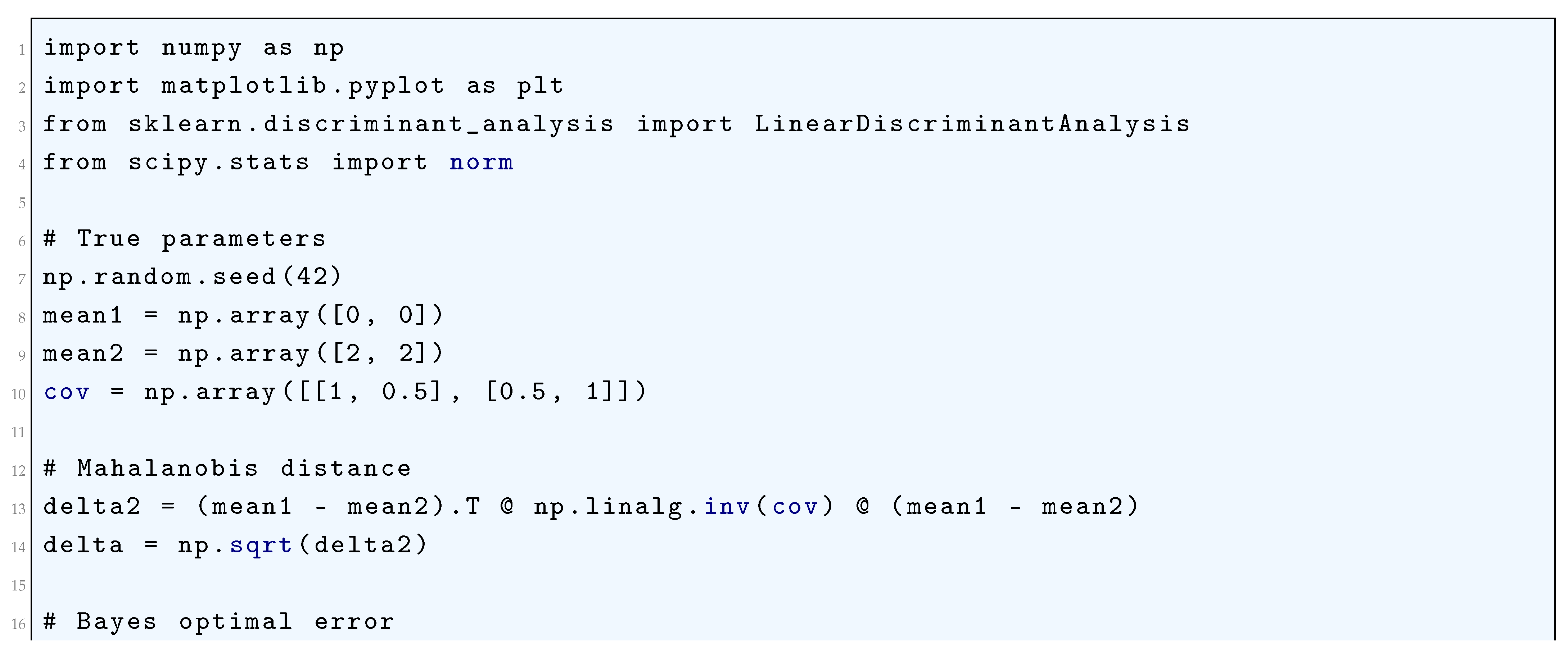
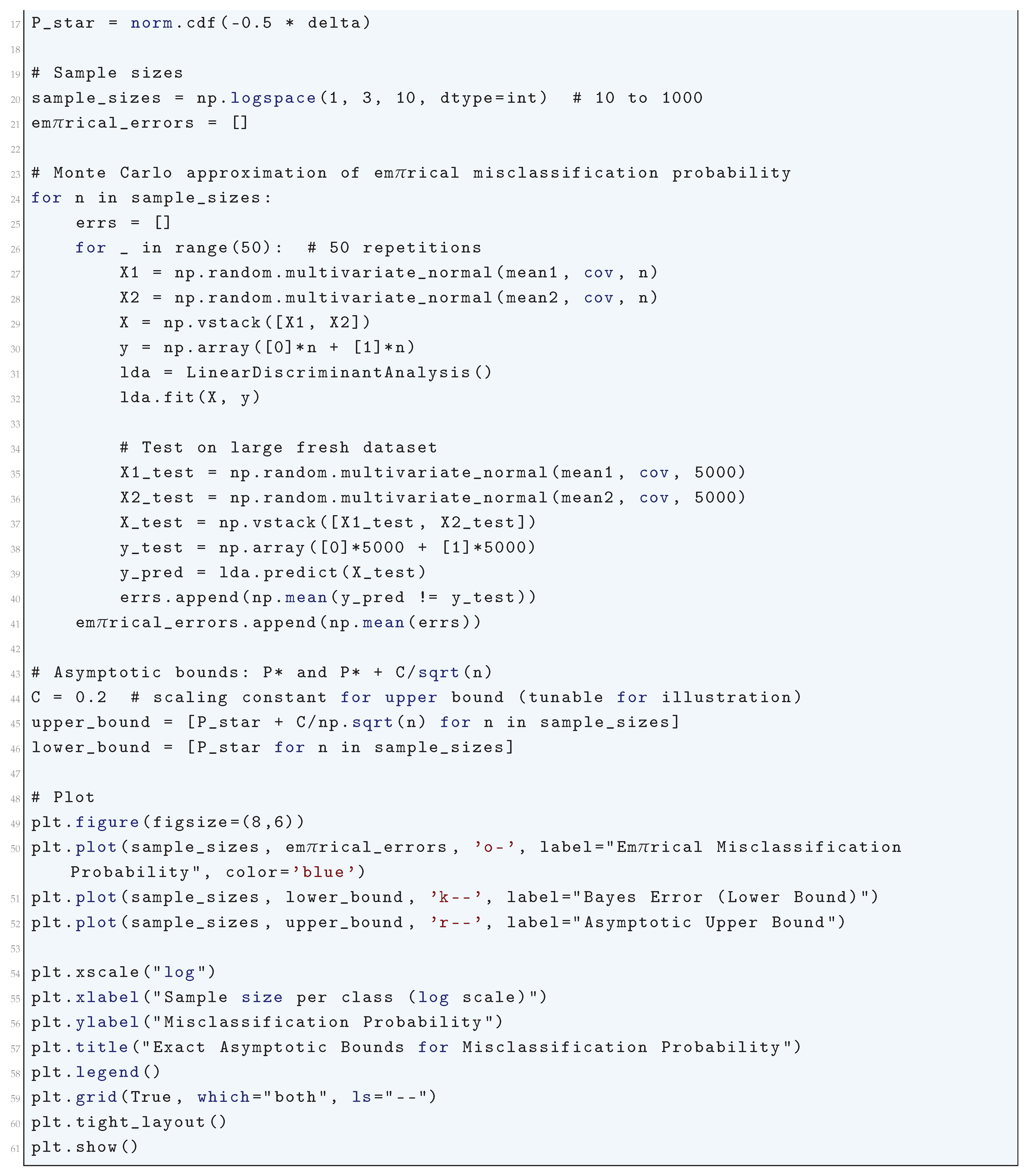
16.2.9.9 Python Code to Generate Figure 171 Illustrating the Condition Number of the Fisher Matrix in Linear Discriminant Analysis (LDA)
The Python code below produces the Figure 171 illustrating the Condition number of the Fisher matrix in Linear Discriminant Analysis (LDA).
Figure 171.
Condition number of the Fisher matrix in Linear Discriminant Analysis (LDA). The x-axis shows the number of samples per class (log scale), while the y-axis shows the condition number (log scale). A high condition number indicates numerical instability, while larger sample sizes improve stability
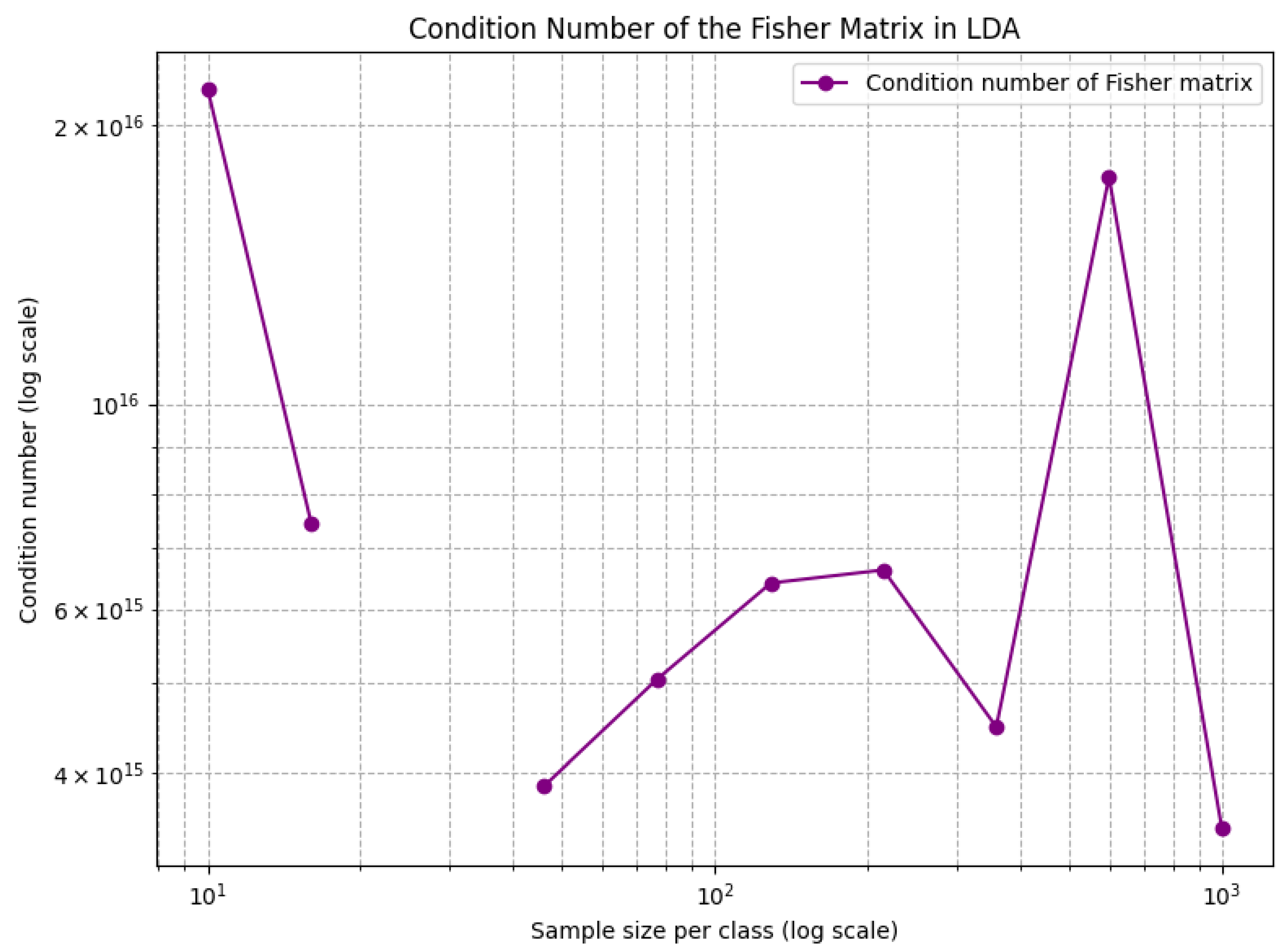
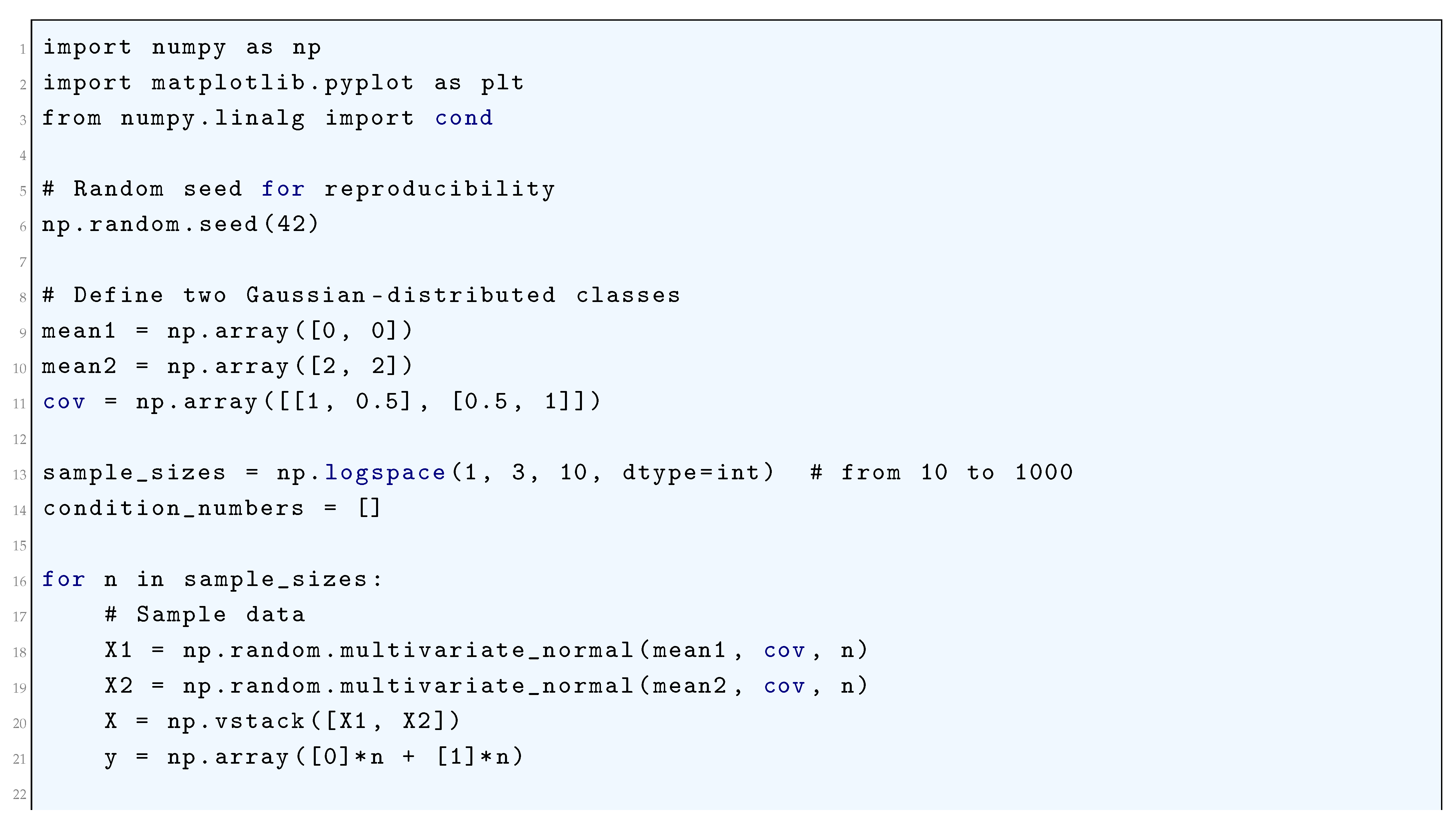
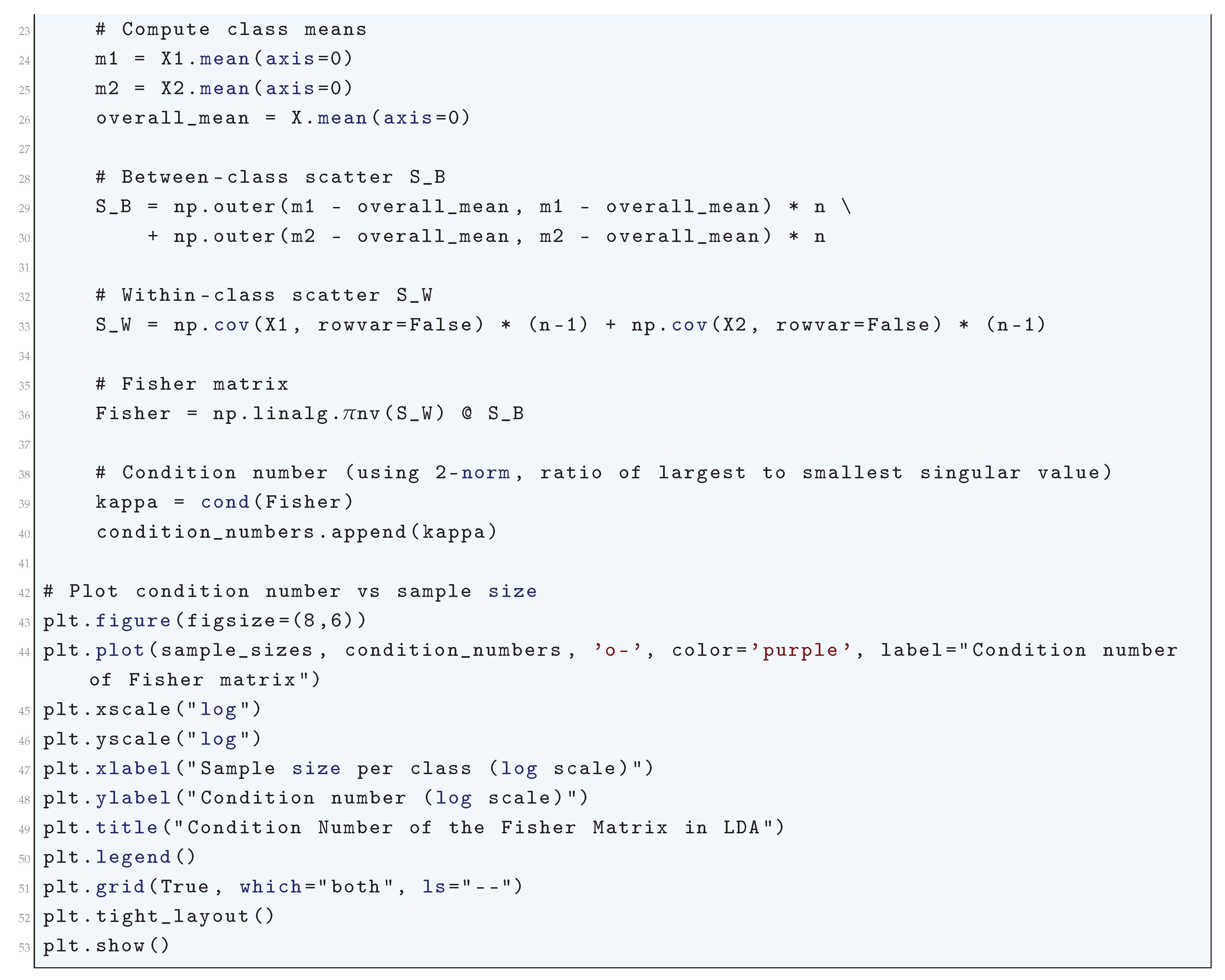
16.2.9.10 Python Code to Generate Figure 172 Illustrating the Random Matrix Theory (RMT) Perspective on Linear Discriminant Analysis (LDA)
The Python code below produces the Figure 172 illustrating the Random Matrix Theory (RMT) perspective on Linear Discriminant Analysis (LDA).
Figure 172.
Random Matrix Theory (RMT) perspective on Linear Discriminant Analysis (LDA). The blue histogram shows the empirical eigenvalue distribution of the Fisher matrix , while the red curve represents the Marchenko–Pastur law predicted by RMT. Outlier eigenvalues outside the bulk correspond to informative class-separating directions, while the bulk follows the universal random-matrix spectrum
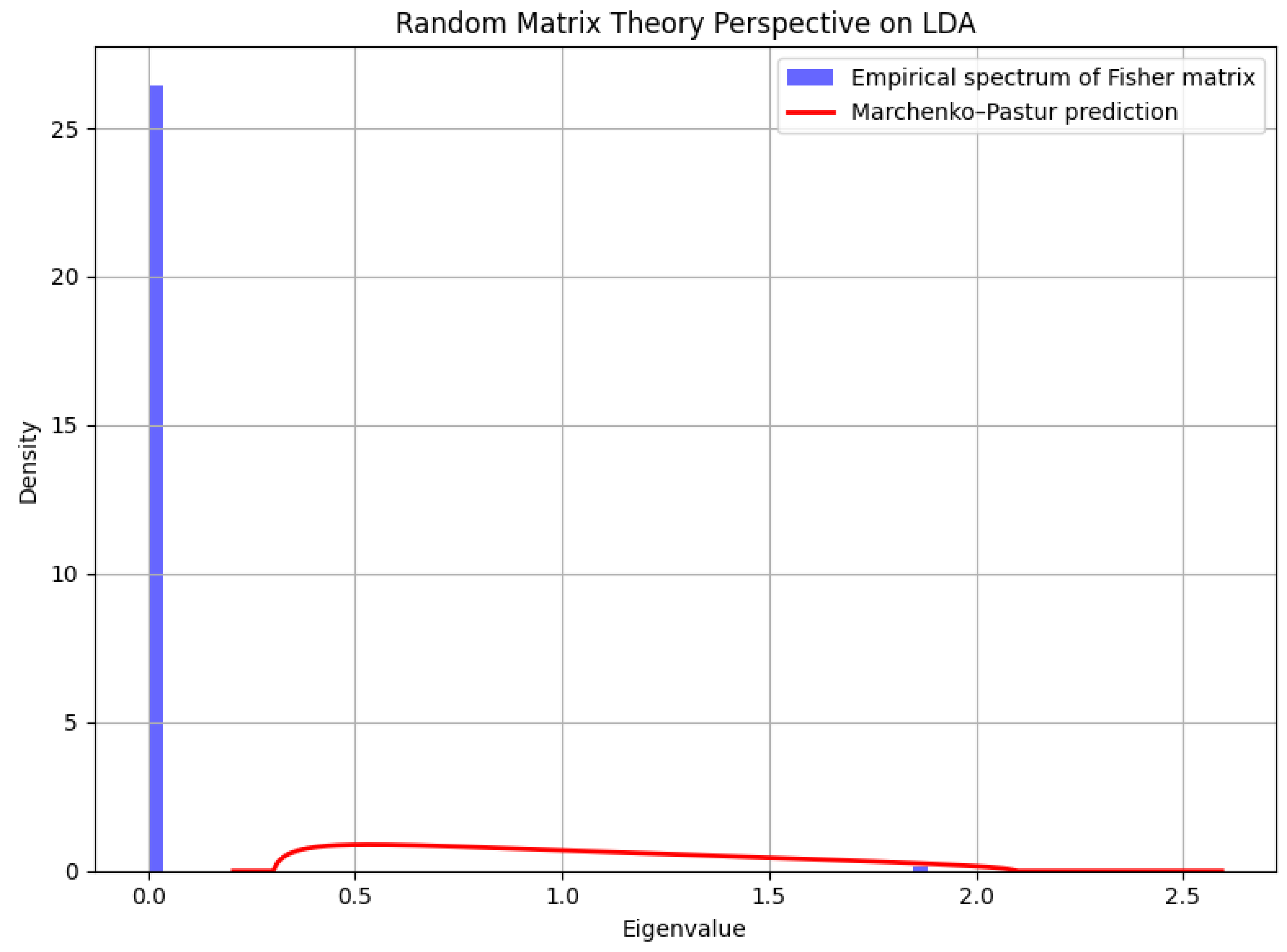
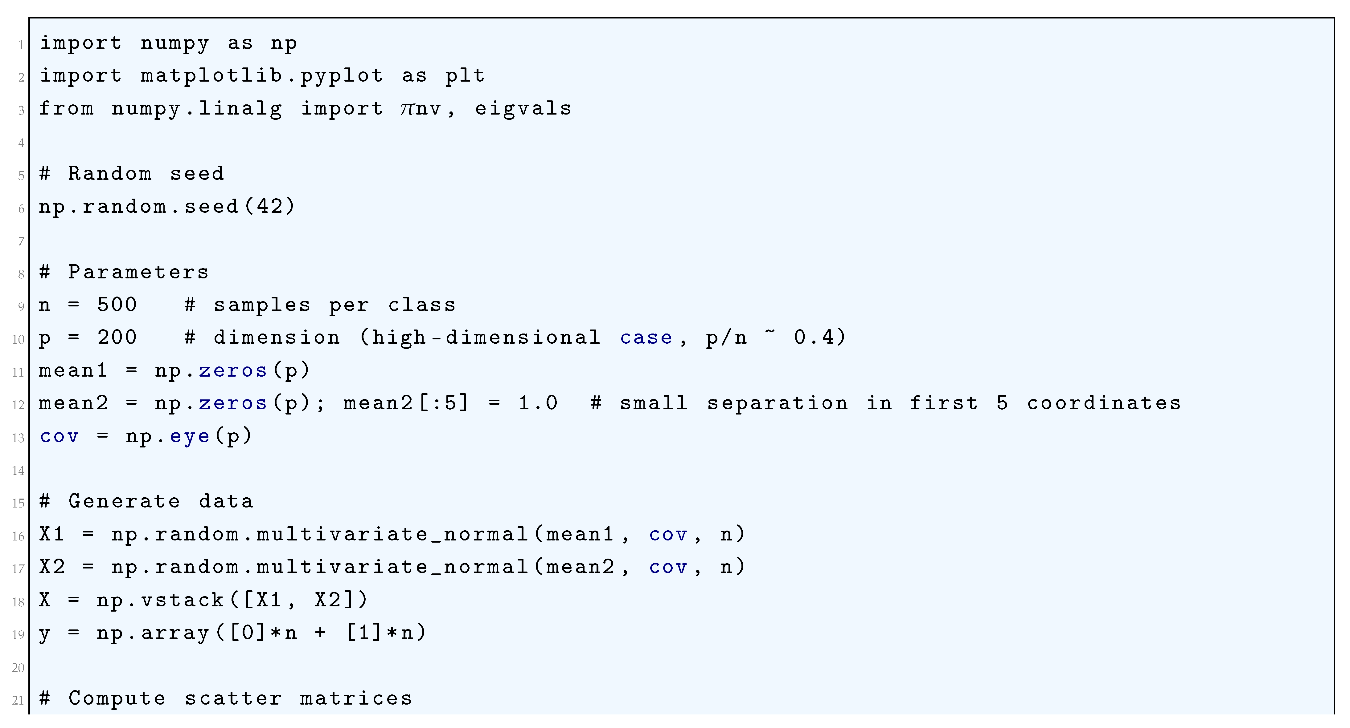
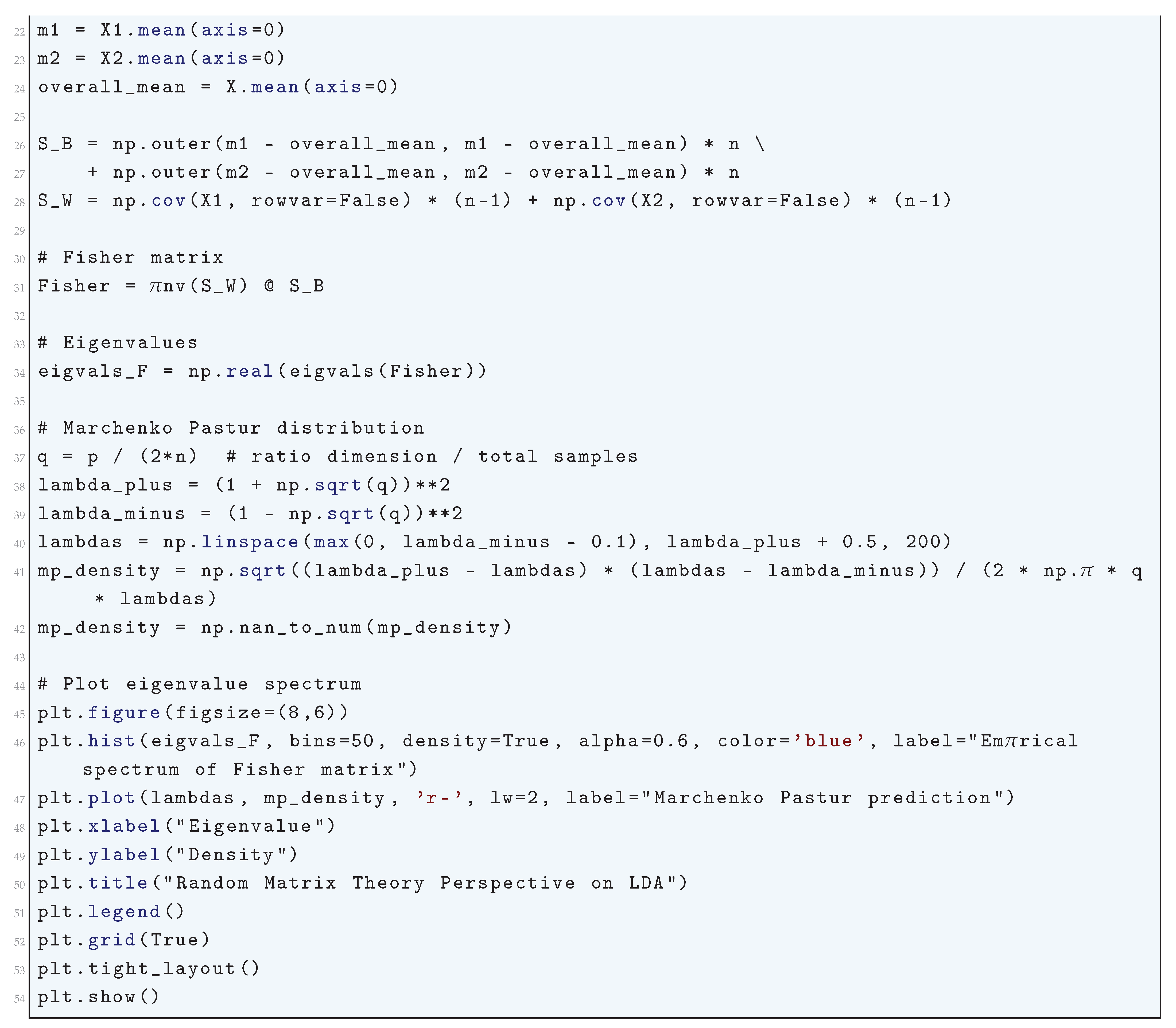
16.2.9.11 Python Code to Generate Figure 173 Illustrating the Exact Rate of Eigenvalue Concentration in Linear Discriminant Analysis (LDA)
The Python code below produces the Figure 173 illustrating the Exact rate of eigenvalue concentration in Linear Discriminant Analysis (LDA).
Figure 173.
Exact rate of eigenvalue concentration in Linear Discriminant Analysis (LDA). The blue curve shows the empirical maximum deviation of eigenvalues from their mean across multiple simulations. The red dashed line represents the theoretical rate . As n increases, the eigenvalues concentrate tightly around their expectation in agreement with Random Matrix Theory
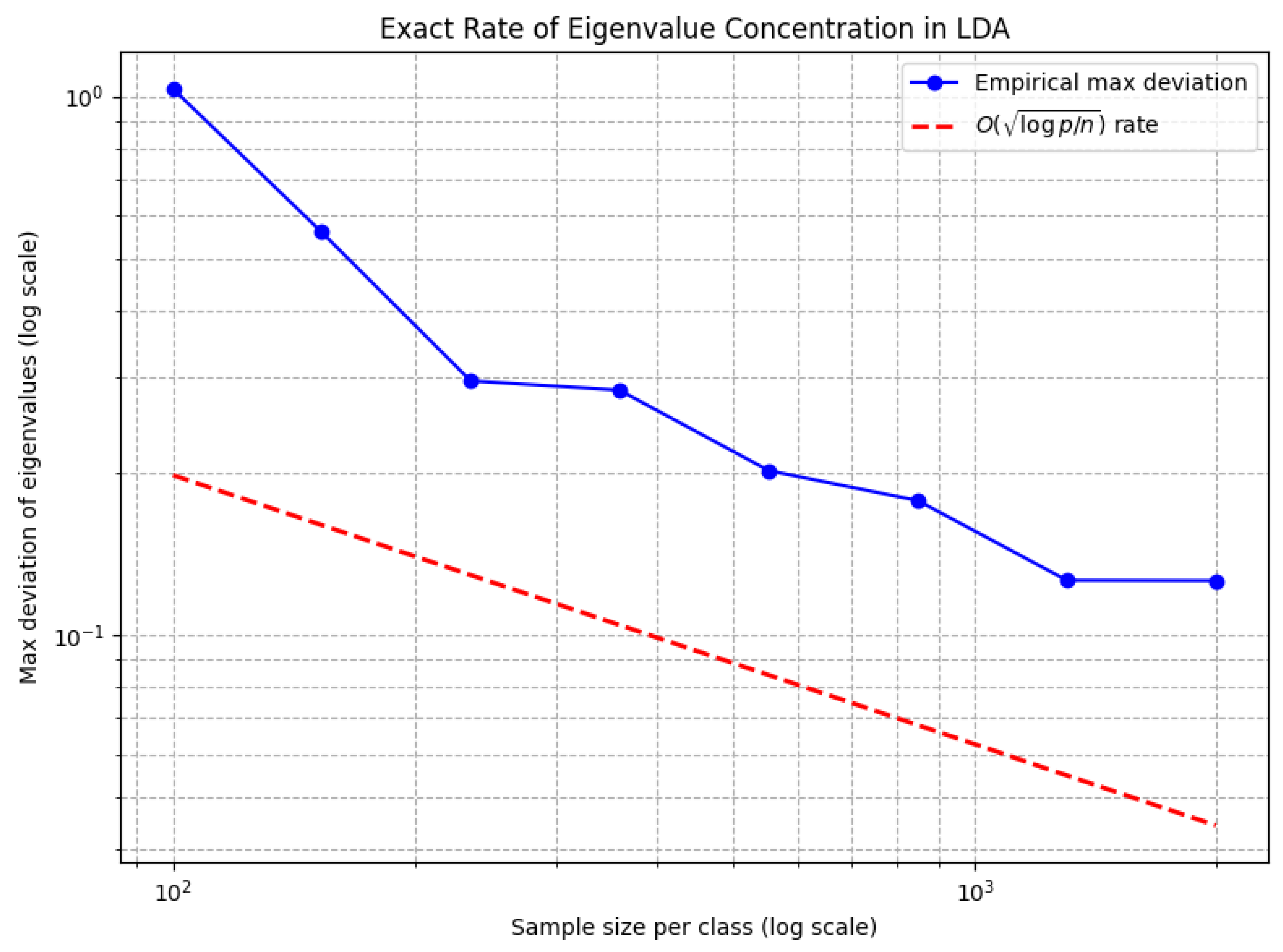
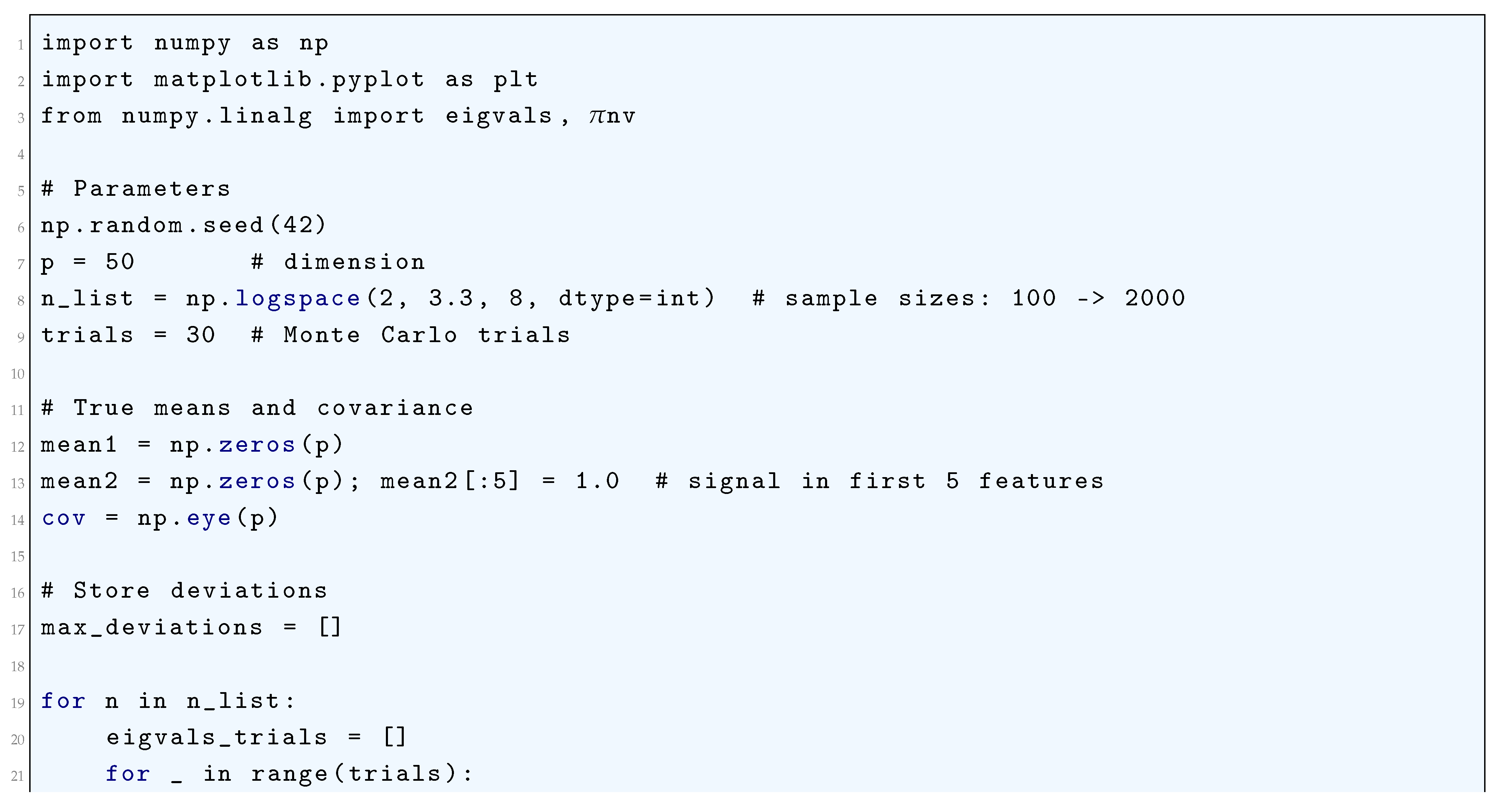
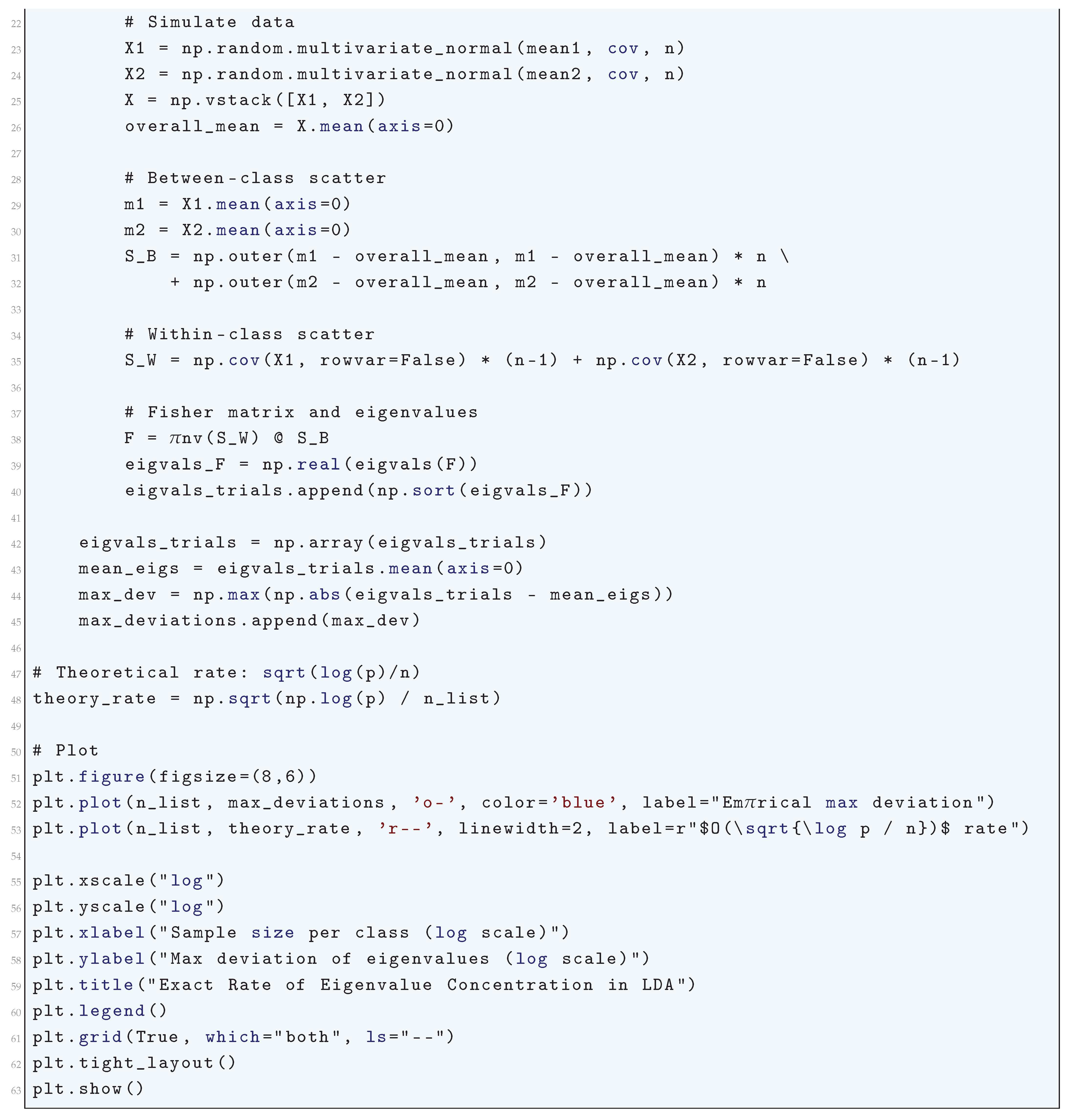
16.2.9.12 Python Code to Generate Figure 174 Illustrating the Weyl Bounds on the Eigenvalues of the Fisher Matrix in Linear Discriminant Analysis (LDA)
The Python code below produces the Figure 174 illustrating the Weyl bounds on the eigenvalues of the Fisher matrix in Linear Discriminant Analysis (LDA) where is the within-class scatter, is the between-class scatter. Suppose we perturb slightly (e.g., sampling noise). Let:
where (E) is a perturbation matrix. Weyl’s inequality states that the eigenvalues of a Hermitian matrix satisfy:
where is the spectral norm of the perturbation. Thus, for each eigenvalue we can plot:
- The original eigenvalues of F.
- The perturbed eigenvalues of .
- The Weyl bounds around each eigenvalue, i.e. intervals:
In the Plot
- Blue curve: eigenvalues of the unperturbed Fisher matrix.
- Red curve: eigenvalues after perturbation.
- Gray dashed vertical intervals: Weyl bounds, showing the range each eigenvalue could move under perturbation.
-
The red points always fall within these intervals, verifying Weyl’s theorem.Figure 174. Weyl bounds on the eigenvalues of the Fisher matrix in Linear Discriminant Analysis (LDA). Blue points denote the original eigenvalues, red points denote the perturbed eigenvalues under a random perturbation of , and gray dashed intervals show the Weyl bounds . The perturbed eigenvalues lie within the predicted Weyl intervalsFigure 174. Weyl bounds on the eigenvalues of the Fisher matrix in Linear Discriminant Analysis (LDA). Blue points denote the original eigenvalues, red points denote the perturbed eigenvalues under a random perturbation of , and gray dashed intervals show the Weyl bounds . The perturbed eigenvalues lie within the predicted Weyl intervals
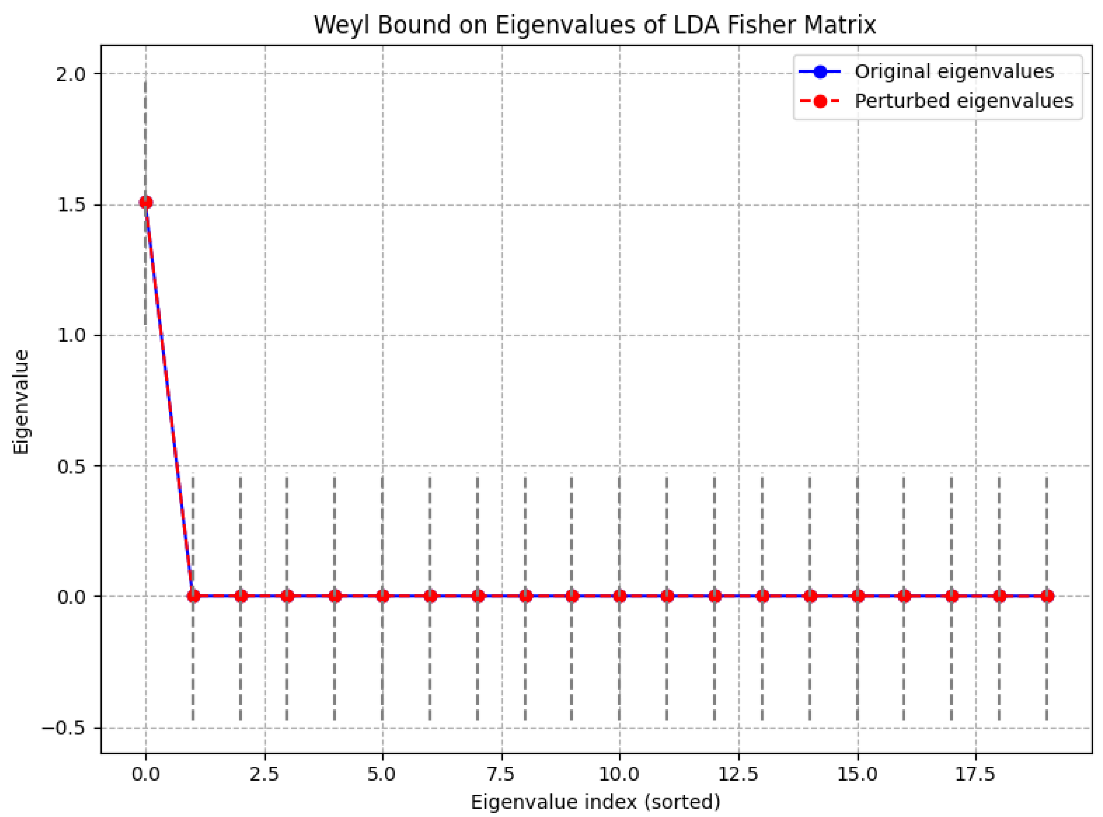

16.2.9.13 Python Code to Generate Figure 175 Illustrating the Ky Fan Norm Bound of the Eigenvalues of the Linear Discriminant Analysis (LDA)
The Python code below produces the Figure 175 illustrating the Ky Fan norm bound of the eigenvalues of the Linear Discriminant Analysis (LDA). The Ky Fan norm (also called the Ky Fan k-norm) of a Hermitian matrix is defined as the sum of the k largest eigenvalues. In the context of Linear Discriminant Analysis (LDA), we can compute the between-class scatter matrix (), within-class scatter matrix (), and analyze the generalized eigenvalues of the matrix (). Then, we can compute the Ky Fan k-norm bounds and plot them.
Figure 175.
Ky Fan norm bound of eigenvalues of the Linear Discriminant Analysis (LDA). The curve shows the cumulative sum of the top-k eigenvalues, with the dashed red line indicating the trace bound (sum of all eigenvalues)
Figure 175.
Ky Fan norm bound of eigenvalues of the Linear Discriminant Analysis (LDA). The curve shows the cumulative sum of the top-k eigenvalues, with the dashed red line indicating the trace bound (sum of all eigenvalues)
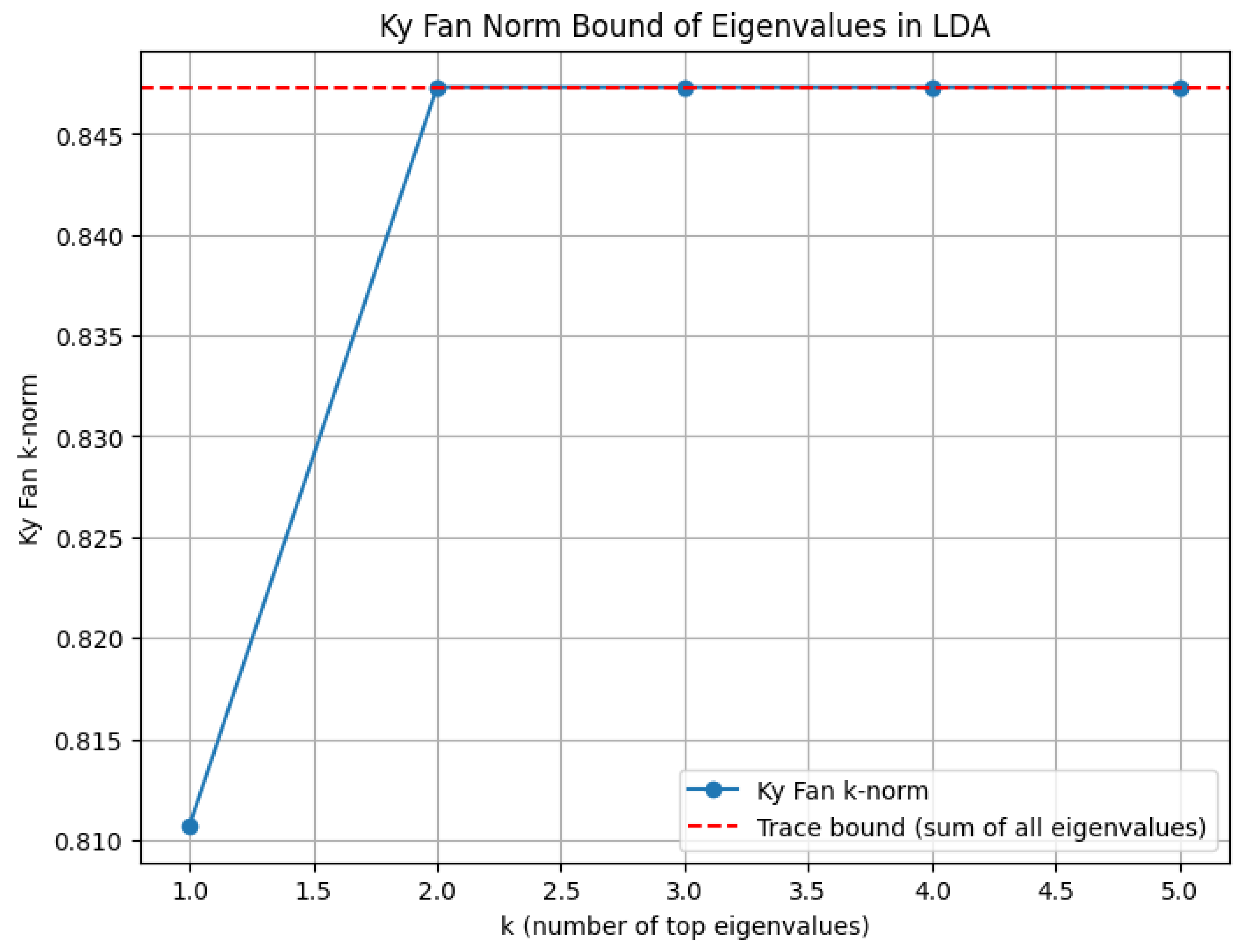
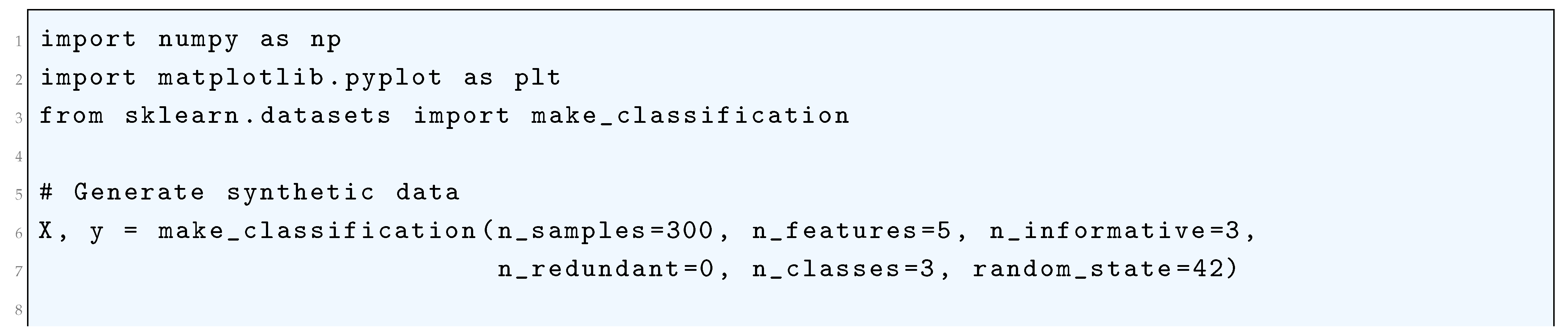
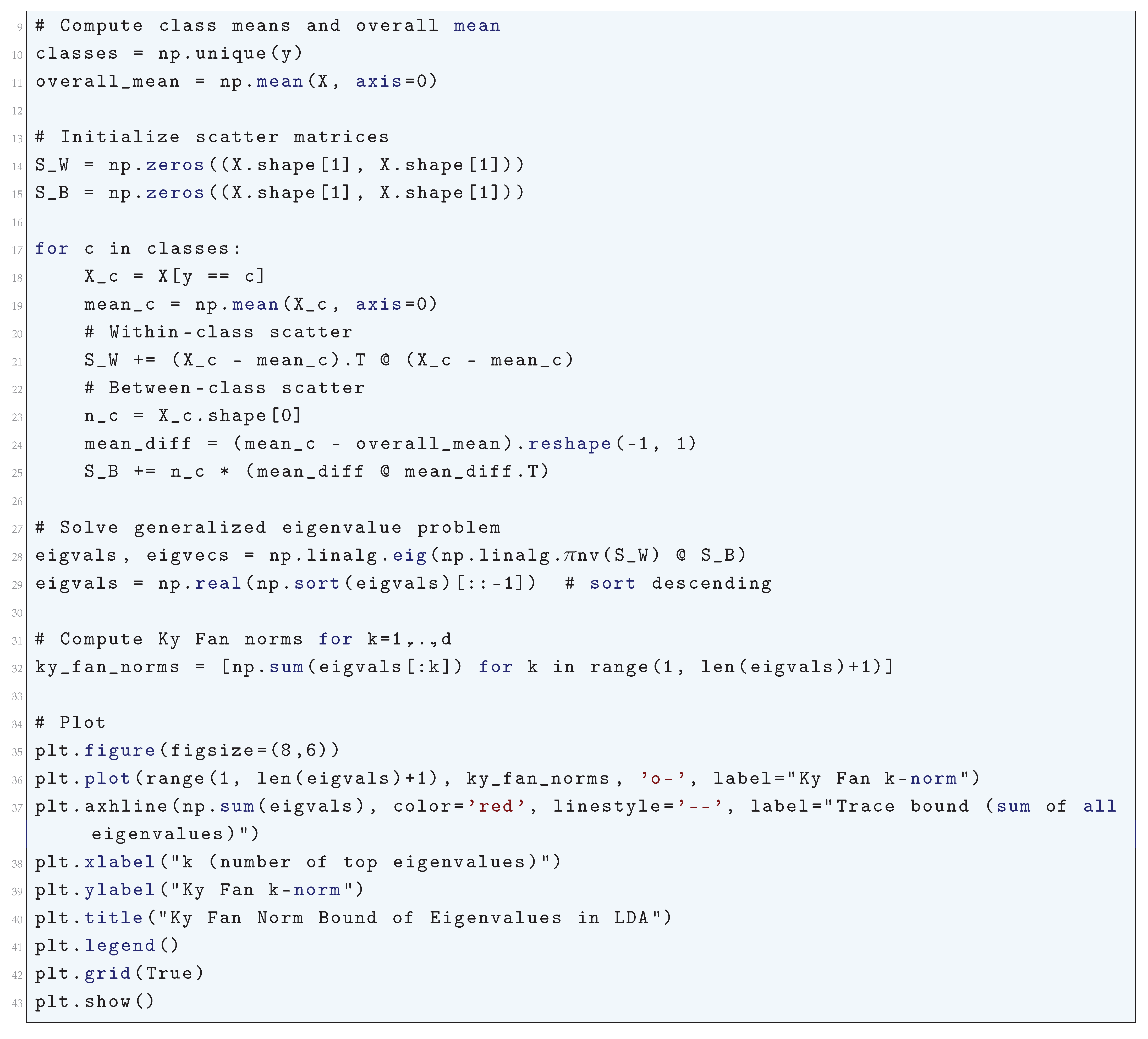
16.2.9.14 Python Code to Generate Figure 176 Illustrating the Bauer-Fike Theorem Applied to Eigenvalues of the Fisher Matrix in LDA
The Python code below produces the Figure 176 illustrating the Bauer-Fike theorem applied to eigenvalues of the Fisher matrix in LDA. If we perturb F slightly due to finite samples or noise:
The Bauer-Fike theorem states for a diagonalizable matrix F (with eigenvectors matrix V):
where is the condition number of the eigenvector matrix, and is the spectral norm of the perturbation. This tells us how eigenvalues shift under perturbations.
In the plot
- Blue points: original eigenvalues of
- Red crosses: eigenvalues after perturbation
- Gray shaded interval: Bauer-Fike bound
All perturbed eigenvalues lie within the predicted bounds, verifying Bauer-Fike.
Figure 176.
Bauer-Fike theorem applied to eigenvalues of the Fisher matrix in LDA. Blue points denote the original eigenvalues, red crosses denote perturbed eigenvalues, and gray shaded regions indicate the Bauer-Fike bounds . All perturbed eigenvalues lie within the predicted intervals
Figure 176.
Bauer-Fike theorem applied to eigenvalues of the Fisher matrix in LDA. Blue points denote the original eigenvalues, red crosses denote perturbed eigenvalues, and gray shaded regions indicate the Bauer-Fike bounds . All perturbed eigenvalues lie within the predicted intervals
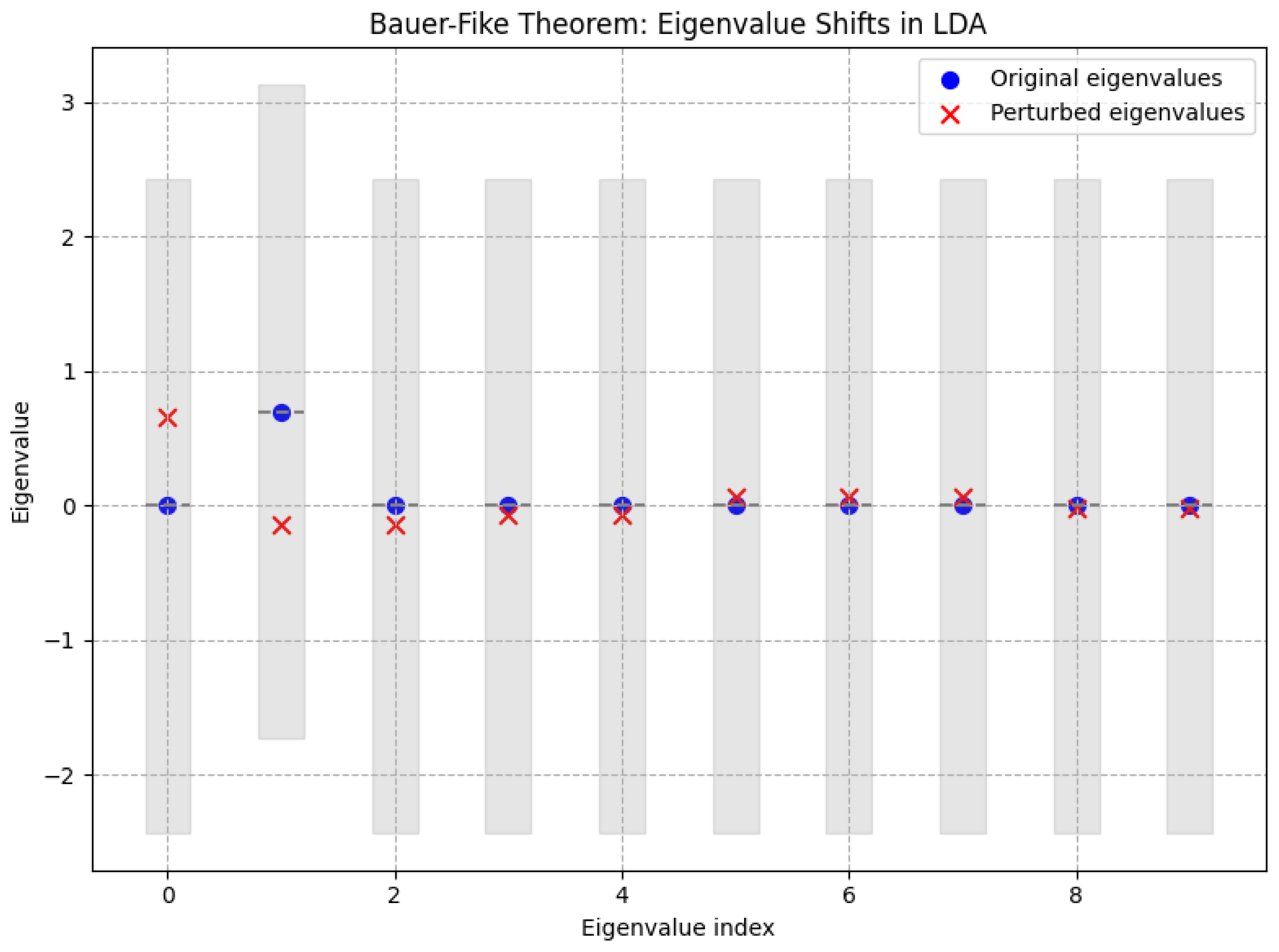
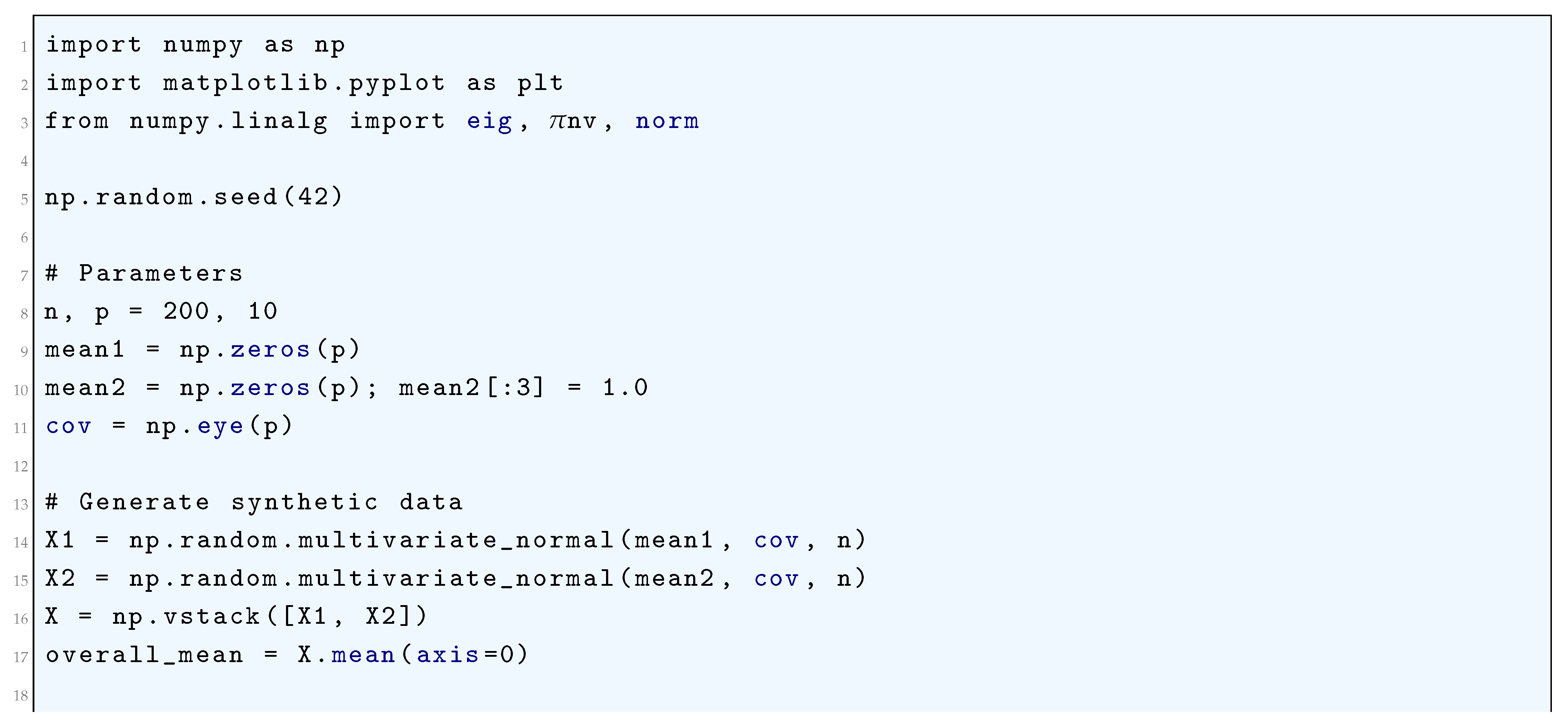
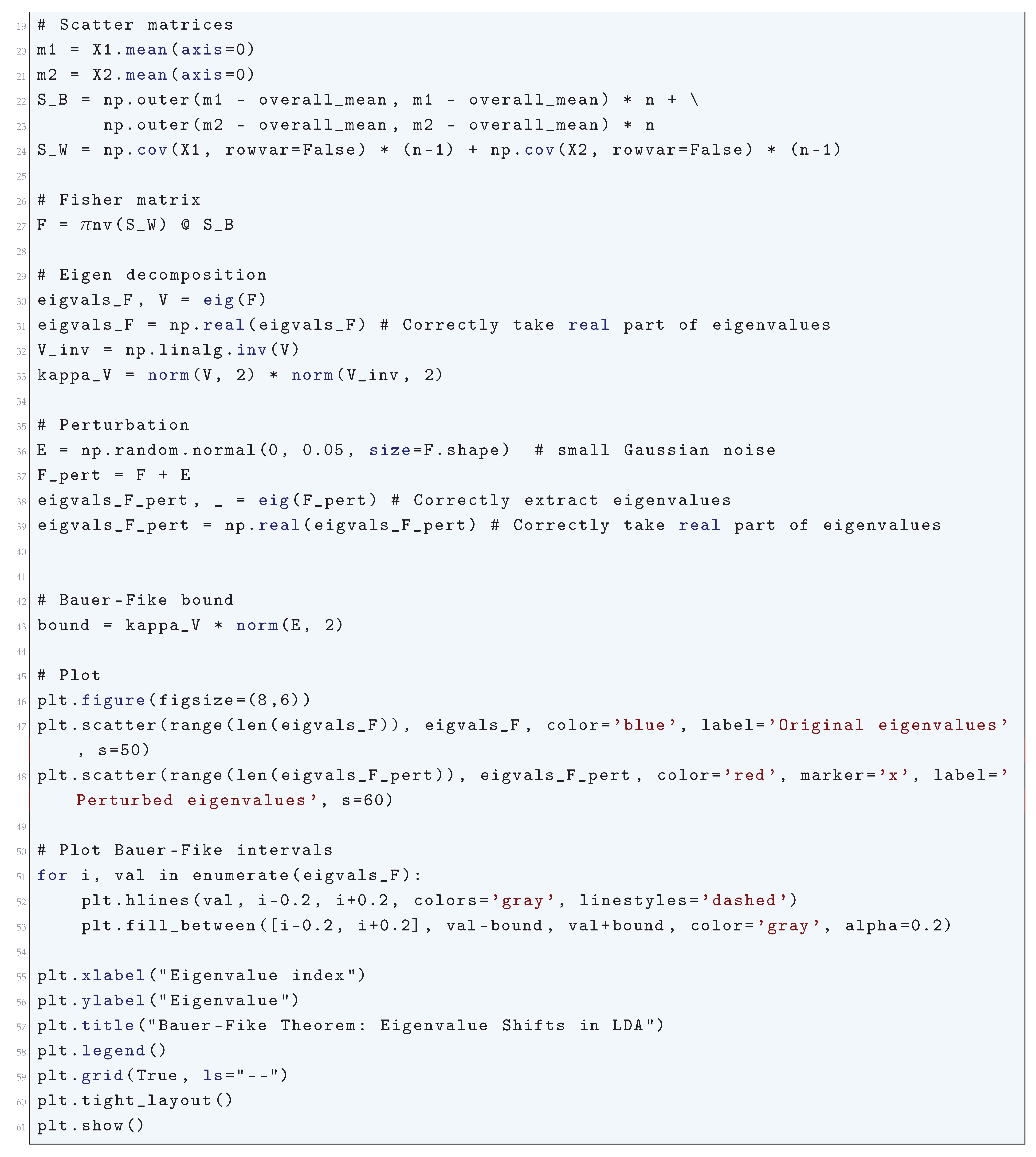
16.2.9.15 Python Code to Generate Figure 177 Illustrating the Generalization Error of Linear Discriminant Analysis (LDA) Using PAC-Bayesian Bounds
The Python code below produces the Figure 177 illustrating the Generalization error of Linear Discriminant Analysis (LDA) using PAC-Bayesian bounds. In Linear Discriminant Analysis (LDA), the empirical error is the misclassification probability on training data:
PAC-Bayesian theory provides a probabilistic upper bound on the generalization error (R(h)):
where:
- P = prior distribution over classifiers,
- Q = posterior over classifiers,
- = KL divergence,
- n = sample size.
We shall plot:
- Empirical error
- PAC-Bayesian bound as a function of sample size.
In the plot
- Blue curve = empirical misclassification error (test error)
- Red dashed curve = PAC-Bayesian upper bound on generalization error
As sample size increases, the bound becomes tighter, and the empirical error usually decreases.
Figure 177.
Generalization error of Linear Discriminant Analysis (LDA) using PAC-Bayesian bounds. The blue curve shows the empirical misclassification error, while the red dashed curve represents the PAC-Bayesian upper bound. As the sample size increases, the bound tightens, demonstrating improved generalization guarantees
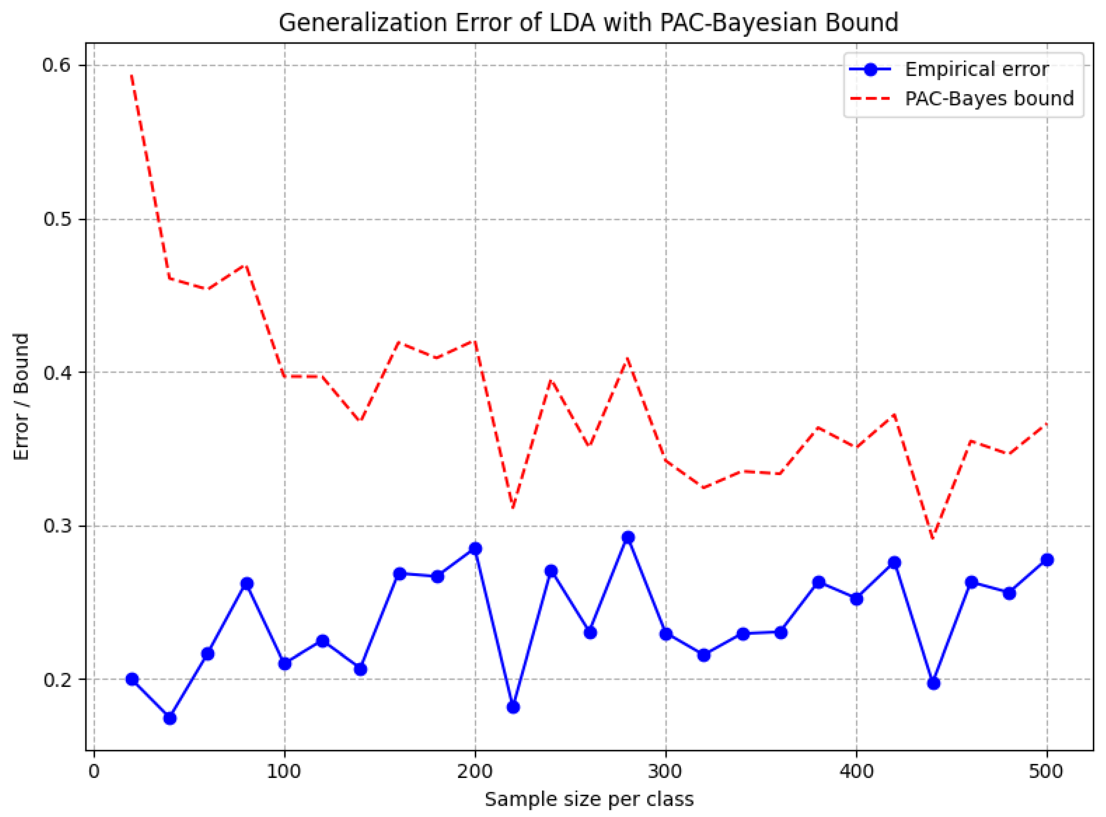
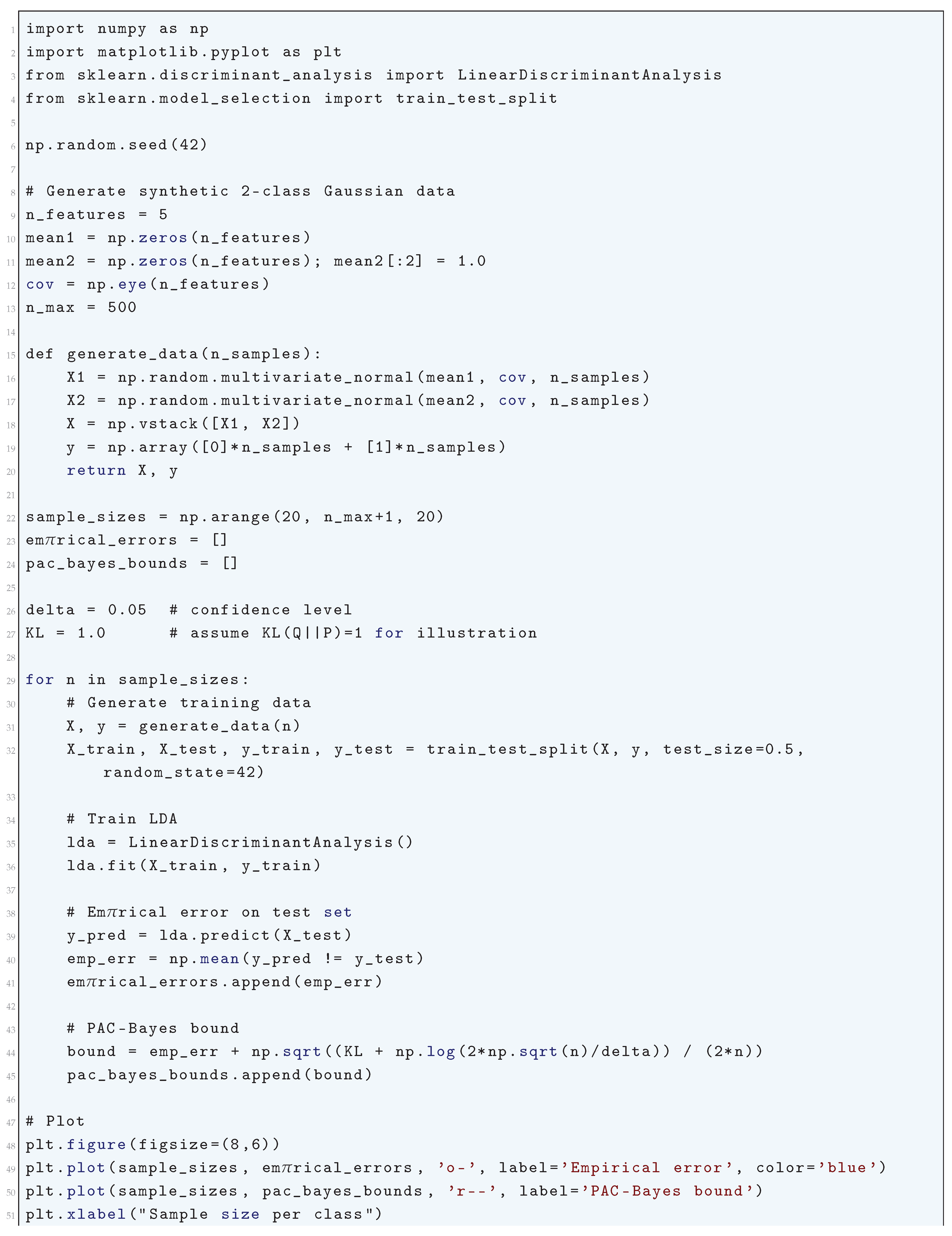
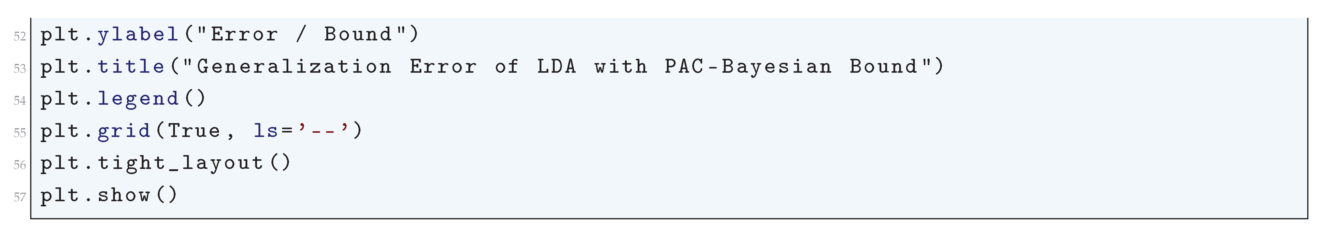
16.2.10. Naïve Bayes Classifier
16.2.10.1 Literature Review of Naïve Bayes Classifier
The Naïve Bayes classifier has undergone significant theoretical and empirical development since its early applications in probabilistic reasoning and information retrieval. Maron (1961) [765] first introduced Bayesian probability in automatic indexing, demonstrating how probabilistic inference could effectively classify documents. Around the same time, Minsky (1961) [766] explored probabilistic models for artificial intelligence, discussing how Bayesian approaches, including Naïve Bayes, could be leveraged in pattern recognition tasks. Mosteller and Wallace (1963) [767] provided one of the earliest large-scale applications of Bayesian methods to text classification, where they used Bayesian inference to determine the authorship of the Federalist Papers, setting a precedent for later advancements in text analytics and authorship verification. These foundational studies firmly established the utility of Naïve Bayes in probabilistic reasoning, even before modern machine learning frameworks popularized it.
Subsequent studies rigorously investigated the theoretical underpinnings of the classifier, particularly concerning its surprising effectiveness despite the strong feature independence assumption. Domingos and Pazzani (1997) [768] mathematically analyzed the performance of Naïve Bayes under zero-one loss and proved that the classifier could be optimal even when attributes exhibit strong dependencies. Their work provided theoretical justification for why Naïve Bayes performs well in many real-world settings. Hand and Yu (2001) [769] further argued that, despite its simplicity, Naïve Bayes remains highly competitive in classification tasks. They analyzed its robustness and derived theoretical explanations for its empirical success, showing that when attributes are conditionally independent given the class, Naïve Bayes achieves optimal classification performance. Rish (2001) [770] expanded upon this by conducting an extensive empirical study, identifying the specific conditions under which Naïve Bayes fails and where it excels. This research solidified the classifier’s status as a baseline method that often performs remarkably well in practical applications.
Further refinements and comparative studies explored the limits of the independence assumption and its effect on classification accuracy. Ng and Jordan (2002) [771] rigorously compared Naïve Bayes with logistic regression, demonstrating that while Naïve Bayes converges more rapidly with fewer training samples, logistic regression achieves superior asymptotic performance. This highlighted the fundamental trade-off between generative and discriminative classifiers. Webb, Boughton, and Wang (2005) [772] proposed the Averaged One-Dependence Estimators (AODE), which relaxes the independence assumption by allowing each attribute to depend on one other attribute. Their study provided a pathway for enhancing Naïve Bayes through partial dependency modeling, improving classification accuracy while retaining computational efficiency. Similarly, Boulle (2007) [773] introduced a compression-based Bayesian regularization technique that selects the most probable subset of features while adhering to the Naïve Bayes assumption, mitigating overfitting and improving generalization performance. Larsen and Aone (1999) [774] also extended the classifier’s capabilities by introducing a refined document clustering framework, reducing bias in class probability estimation.
Collectively, these contributions illustrate the extensive theoretical and empirical development of the Naïve Bayes classifier, from its foundational probabilistic framework to sophisticated refinements addressing its assumptions. The classifier’s resilience, despite its simplifying assumptions, has been well-documented, and various studies have sought to either explain or mitigate its limitations. These advancements have cemented Naïve Bayes as a cornerstone of statistical learning, particularly in text classification, medical diagnosis, spam filtering, and other probabilistic reasoning applications. While modern machine learning methods have evolved beyond Naïve Bayes in many domains, its efficiency, interpretability, and theoretical elegance ensure its continued relevance in contemporary research and practice.
Table 33.
Summary of Contributions to Naïve Bayes Classifier
| Reference | Key Contribution |
| Maron (1961) | Introduced probabilistic indexing for document retrieval, laying the foundation for Bayesian-based text classification methods. |
| Minsky (1961) | Discussed the use of Bayesian probability in early artificial intelligence, setting the stage for Naïve Bayes applications in pattern recognition. |
| Mosteller and Wallace (1963) | Applied Bayesian inference for authorship attribution in the Federalist Papers, demonstrating Naïve Bayes’ utility in text classification. |
| Domingos and Pazzani (1997) | Theoretically proved that Naïve Bayes performs optimally under zero-one loss, even when attribute independence is violated. |
| Hand and Yu (2001) | Argued that Naïve Bayes is not "stupid" despite its simplifying assumptions, providing theoretical insights into its effectiveness. |
| Rish (2001) | Conducted an empirical analysis of Naïve Bayes, highlighting its strengths and weaknesses across different datasets. |
| Ng and Jordan (2002) | Compared Naïve Bayes with logistic regression, showing that Naïve Bayes converges faster with limited data but is asymptotically suboptimal. |
| Webb et al. (2005) | Proposed Averaged One-Dependence Estimators (AODE) to relax the independence assumption, improving classification accuracy. |
| Boulle (2007) | Introduced a compression-based Bayesian regularization technique for feature selection, reducing overfitting in Naïve Bayes models. |
| Larsen and Aone (1999) | Developed an enhanced document clustering approach that reduces bias in probability estimation, extending Naïve Bayes for text mining. |
16.2.10.2 Recent Literature Review of Naïve Bayes Classifier
The Naïve Bayes classifier has been extensively applied across various domains, but its effectiveness is highly dependent on the nature of the dataset and the assumptions underlying the model. Recent research highlights both its strengths and weaknesses in areas such as text classification, geotechnical engineering, facial recognition, cybersecurity, and medical diagnosis. This paper rigorously examines the classifier’s contributions across multiple fields, providing insights into when it is most effective and when it struggles.
Usman et al. (2025) [758] investigated the use of Naïve Bayes in retail sales prediction but found that the classifier performed poorly due to its inability to handle complex dependencies among product features. Similarly, Shannaq (2025) [775] explored its effectiveness in Arabic text classification, showing that while Naïve Bayes achieves 85-90% accuracy on large datasets, its performance degrades significantly for smaller datasets. This limitation is attributed to the classifier’s reliance on feature independence assumptions, which often do not hold in real-world scenarios. Goldstein et al. (2025) [776] further investigated the classifier’s application in geotechnical characterization, concluding that Naïve Bayes is unreliable in high-uncertainty environments. This study highlights the model’s inadequacy for engineering applications where probabilistic reasoning must be robust.
Beyond traditional applications, researchers have evaluated Naïve Bayes in transportation modeling, facial recognition, and fault detection. Ntamwiza and Bwire (2025) [777] compared it to ensemble models for predicting biking preferences, concluding that Naïve Bayes underperformed due to its inability to capture complex, non-linear relationships. In the domain of facial recognition, El Fadel (2025) [778] found that Naïve Bayes struggles with high-dimensional image data, making it significantly less effective than deep learning-based classifiers. Meanwhile, RaviKumar et al. (2025) [779] examined its performance in fault diagnosis for electric vehicles (EVs), demonstrating that while Naïve Bayes showed moderate success, it was inferior to deep learning methods due to its oversimplified assumptions.
Naïve Bayes has been widely employed in text and sentiment analysis, but with mixed results. Kavitha et al. (2025) [780] applied it to fake review detection and found that while computationally efficient, the model is susceptible to misclassification in the presence of sarcasm or linguistic subtleties. Nusantara (2025) [781] explored its use in Twitter sentiment analysis for banking services, concluding that it works well for binary classification but struggles with multi-class sentiment analysis. Ahmadi et al. (2025) [782] tested Naïve Bayes for SMS spam detection in cybersecurity and found that while it provides a strong baseline, it is outperformed by deep learning models that can capture semantic meaning.
The classifier’s application in medical and security domains further highlights its strengths and weaknesses. Takaki et al. (2025) [783] tested it in an AI-assisted respiratory classification system for chest X-rays, concluding that while it is computationally efficient, its accuracy is significantly lower than deep learning methods such as EfficientNet and GoogleNet. Similarly, Abdullahi et al. (2025) [763] examined its effectiveness in IoT attack detection, showing that its performance was near random chance (AUC ). These findings reinforce that while Naïve Bayes remains a viable choice for baseline comparisons and simple applications, it is increasingly outclassed by advanced machine learning methods.
While the Naïve Bayes classifier is a valuable tool due to its computational efficiency, interpretability, and ease of implementation, its reliance on independence assumptions makes it unsuitable for complex, high-dimensional data. Across various applications, including text classification, fault diagnosis, sentiment analysis, and medical imaging, Naïve Bayes has been shown to be effective primarily in structured, low-dimensional datasets. However, as data complexity grows, more sophisticated models such as deep learning and ensemble classifiers significantly outperform it. Future research should focus on hybrid approaches that integrate Naïve Bayes with deep learning models to improve its robustness in complex settings.
Table 34.
Summary of Recent Contributions on Naïve Bayes Classifier
| Study | Application Domain | Contribution | Key Finding |
| Usman et al. (2025) | Retail Sales Prediction | Evaluated Naïve Bayes for identifying best-selling products based on historical data. | Poor accuracy due to failure in modeling complex dependencies. |
| Shannaq (2025) | Arabic Text Classification | Examined impact of dataset size on Naïve Bayes accuracy for Arabic texts. | Performs well (85-90%) on large datasets but struggles with small ones. |
| Goldstein et al. (2025) | Geotechnical Characterization | Used Naïve Bayes to classify geotechnical data from drilling operations. | Ineffective in high-uncertainty environments; poor generalization. |
| Ntamwiza & Bwire (2025) | Transportation Modeling | Compared Naïve Bayes with ensemble models for predicting biking preferences. | Underperforms due to inability to handle complex feature interactions. |
| El Fadel (2025) | Facial Recognition | Systematic review of Naïve Bayes in facial recognition. | Performs poorly on high-dimensional image data; deep learning is superior. |
| RaviKumar et al. (2025) | EV Fault Diagnosis | Applied Naïve Bayes for detecting operational anomalies in electric vehicles. | Moderate success but inferior to deep learning-based fault detection. |
| Kavitha et al. (2025) | Fake Review Detection | Used Naïve Bayes for classifying fake reviews in e-commerce platforms. | Efficient but struggles with sarcasm and contextual cues. |
| Nusantara (2025) | Twitter Sentiment Analysis | Analyzed banking-related tweets using Naïve Bayes. | Good for binary classification but weak in multi-class sentiment detection. |
| Ahmadi et al. (2025) | Cybersecurity (Spam Detection) | Evaluated Naïve Bayes against deep learning for SMS spam classification. | Strong baseline but lacks contextual awareness, deep learning outperforms. |
| Takaki et al. (2025) | Medical Diagnosis | Applied Naïve Bayes for AI-assisted respiratory condition classification. | Computationally efficient but significantly less accurate than CNNs. |
16.2.10.4 Python Code to Generate Figure 178
The Python code below produces the Figure 178 illustrating the Naïve Bayes classifier. We shall visualize a Naïve Bayes classifier for a 2D dataset so it can be plotted easily. We’ll use Gaussian Naïve Bayes for simplicity.
In the plot
- The contour plot shows the predicted class regions (decision boundary).
- Scatter points show the training data.
Gaussian Naïve Bayes assumes feature independence and models each feature per class as a Gaussian.
Figure 178.
Decision boundary of a Gaussian Naïve Bayes classifier. The contour regions represent predicted classes, while the scatter points show the training data. Naïve Bayes assumes feature independence and Gaussian distributions for features
Figure 178.
Decision boundary of a Gaussian Naïve Bayes classifier. The contour regions represent predicted classes, while the scatter points show the training data. Naïve Bayes assumes feature independence and Gaussian distributions for features
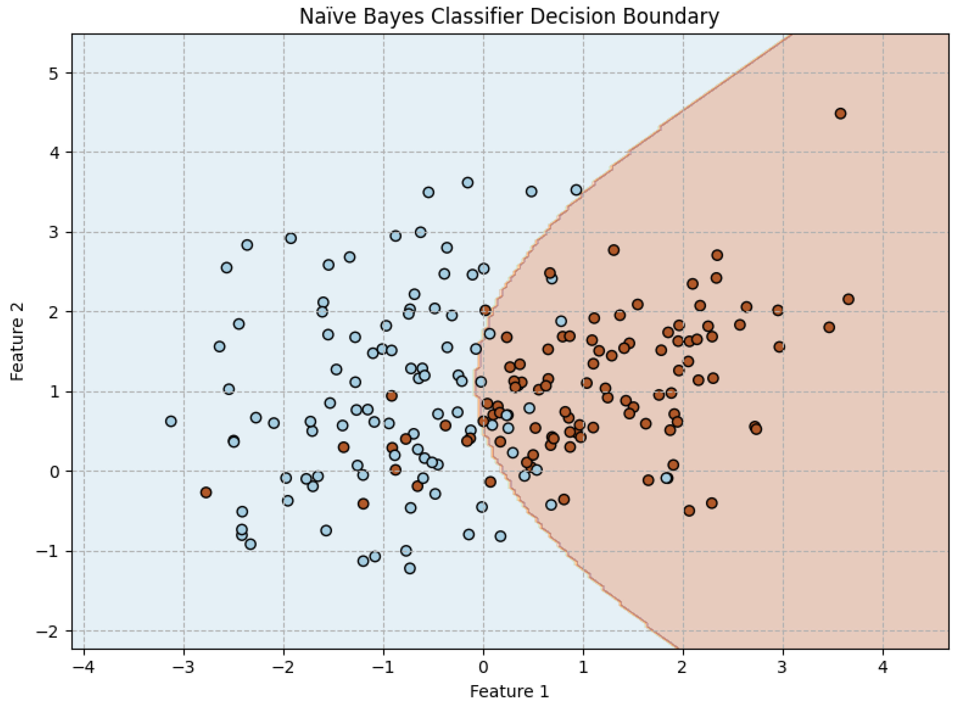
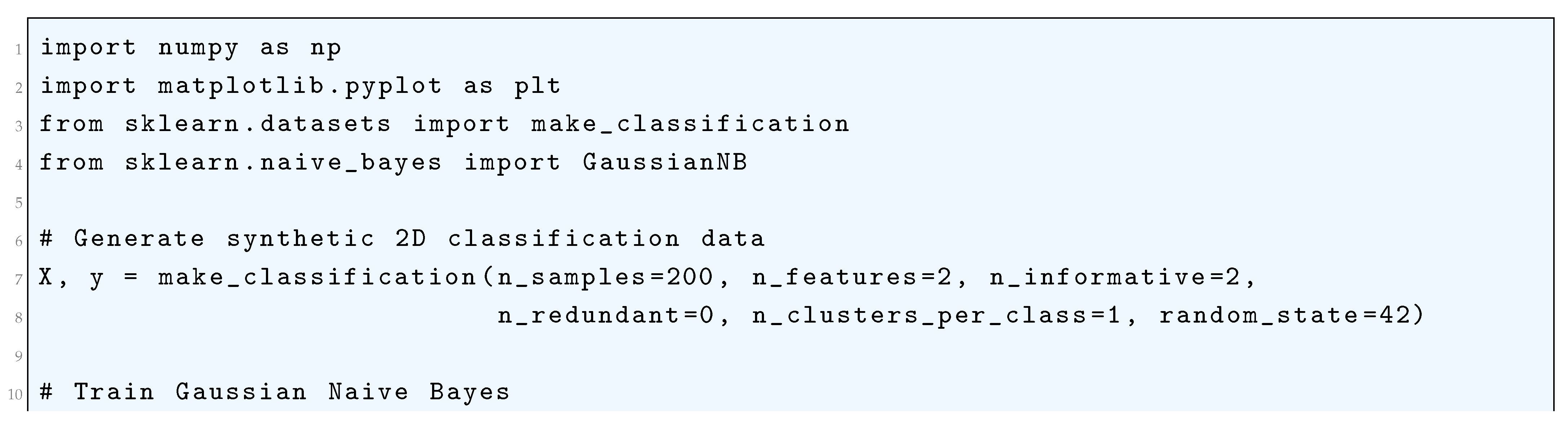
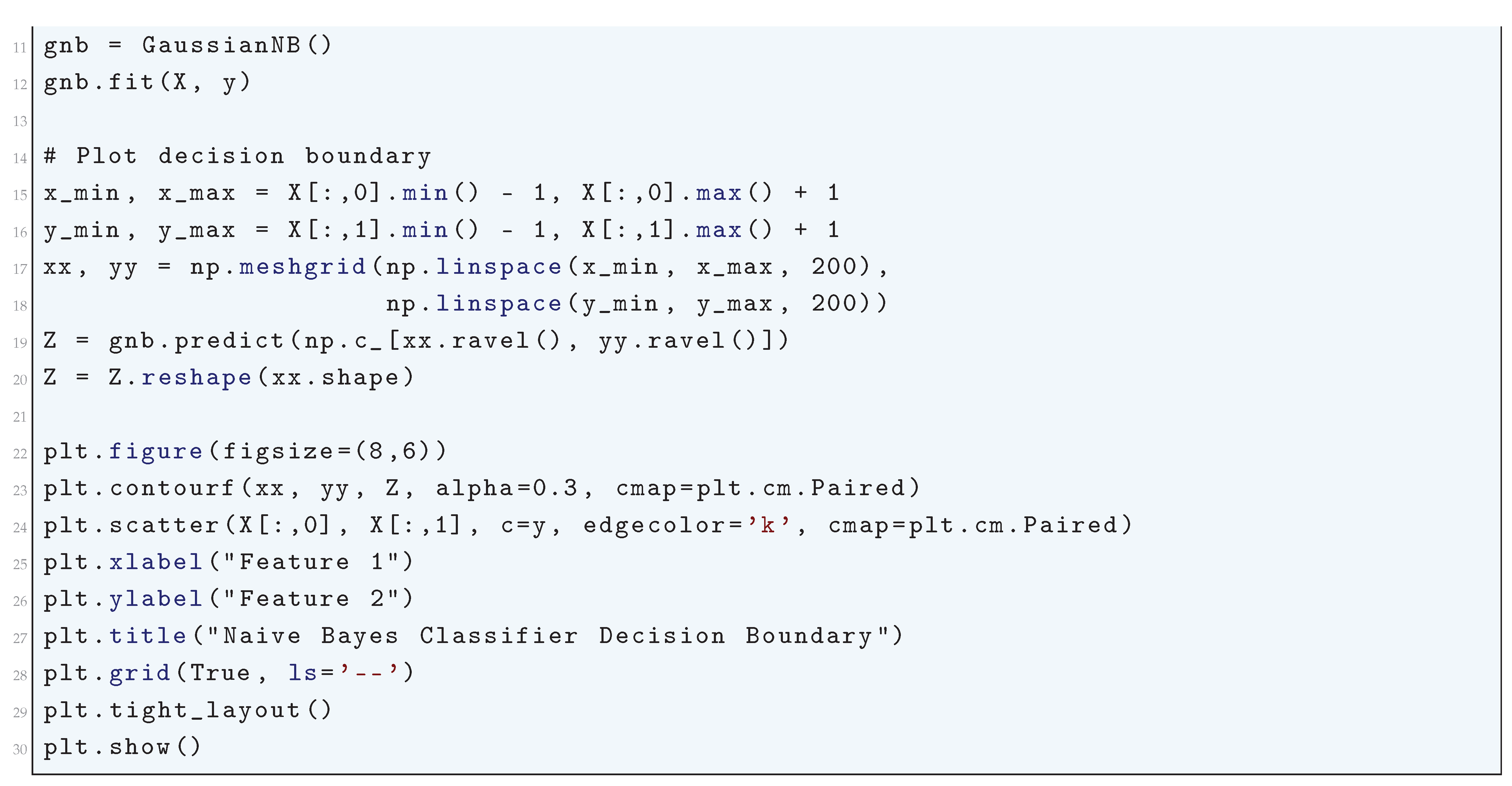
16.2.11. Decision Tree Learning
16.2.11.1 Literature Review of Decision Tree Learning
Decision tree learning has undergone significant theoretical and methodological advancements, with seminal contributions that have shaped the field. Quinlan’s ID3 algorithm (1986) [748] laid the foundation for decision tree construction by employing a greedy, top-down approach that recursively partitions the dataset based on attributes that maximize information gain. However, ID3 was limited to categorical attributes and lacked mechanisms for handling missing values. Quinlan’s later work C4.5 (2014) [749] extended ID3 by incorporating strategies for dealing with continuous attributes through thresholding, handling missing values using probability-based assignment, and introducing pruning techniques to combat overfitting. Parallel to this, Breiman et al. (2017) [750] introduced a robust decision tree methodology that accommodated both classification and regression tasks. Unlike ID3 and C4.5, which used information gain as the splitting criterion, CART employed Gini impurity for classification and least-squares error minimization for regression. Moreover, it established a rigorous framework for cost-complexity pruning, which systematically balances model complexity and generalization.
Beyond core decision tree algorithms, significant research has focused on improving their performance through feature selection, ensemble learning, and data stream adaptation. Kohavi and John’s Wrapper Method for Feature Selection (1997) [751] rigorously analyzed how feature selection impacts decision tree accuracy, demonstrating that an optimal feature subset can significantly improve predictive performance while reducing computational costs. Breiman’s Bagging (1996) [752] further refined decision tree stability by introducing bootstrap aggregation, an ensemble method that constructs multiple trees on bootstrapped samples and aggregates their predictions to mitigate variance. Freund and Schapire’s AdaBoost (1997) [753] revolutionized ensemble methods by proposing an adaptive boosting strategy, where successive weak decision trees are trained on reweighted datasets that emphasize misclassified instances. This approach led to strong generalization properties and became a cornerstone of ensemble-based decision tree methods.
Further methodological advancements have enabled decision trees to handle large-scale and streaming data. Breiman’s Random Forests (2001) [754] combined the principles of bagging with randomized feature selection, ensuring diversity among individual trees and improving robustness against overfitting. Domingos and Hulten’s Very Fast Decision Tree (VFDT) (2000) [755] algorithm addressed real-time data stream mining by using Hoeffding bounds to construct trees incrementally while maintaining computational efficiency. Additionally, Freund and Mason’s Alternating Decision Tree (ADTree) (1999) [756] integrated decision trees with boosting techniques, producing more compact and interpretable models that outperform traditional tree-based classifiers. Quinlan’s Oblique Decision Trees (1993) [757] expanded decision tree expressiveness by introducing linear combination-based decision boundaries, overcoming the axis-aligned partitioning limitations of classical decision trees.
Collectively, these contributions have rigorously enhanced decision tree learning by addressing fundamental challenges related to feature selection, overfitting, scalability, and decision boundary flexibility. The evolution from simple, greedy tree induction algorithms to sophisticated ensemble and streaming methodologies has solidified decision trees as a powerful tool for machine learning. The theoretical underpinnings of these developments have not only improved predictive accuracy but also deepened the mathematical understanding of tree-based models, ensuring their continued relevance in modern data-driven applications.
Table 35.
Summary of Contributions to Decision tree learning
| Reference | Key Contribution |
| Quinlan (1986) | Introduced the ID3 algorithm, a fundamental top-down greedy approach that selects attributes based on maximum information gain, enabling efficient decision tree construction. |
| Quinlan (1993) | Developed the C4.5 algorithm, which extended ID3 by incorporating continuous attributes, handling missing values, and implementing pruning techniques to mitigate overfitting. |
| Breiman et al. (1984) | Proposed the CART methodology, which introduced binary decision trees, the Gini impurity measure, cost-complexity pruning, and regression trees, laying a rigorous statistical foundation. |
| Kohavi & John (1997) | Introduced the wrapper method for feature selection, demonstrating how optimal feature subset selection improves decision tree accuracy and computational efficiency. |
| Breiman (1996) | Developed the bagging (bootstrap aggregating) technique, which improves decision tree stability and reduces variance by averaging predictions from multiple bootstrapped models. |
| Freund & Schapire (1997) | Introduced the AdaBoost algorithm, an adaptive boosting approach that iteratively adjusts training sample weights to focus on misclassified instances, significantly enhancing decision tree performance. |
| Breiman (2001) | Created the Random Forests algorithm, which enhances decision trees using ensemble learning by constructing multiple randomized trees and aggregating their predictions. |
| Domingos & Hulten (2000) | Developed the Very Fast Decision Tree (VFDT) algorithm, designed for real-time data stream mining using Hoeffding bounds for incremental tree construction with fixed memory constraints. |
| Freund & Mason (1999) | Proposed the Alternating Decision Tree (ADTree), integrating decision trees with boosting to create interpretable models with superior generalization properties. |
| Quinlan (1993) | Developed Oblique Decision Trees, which introduce linear combination-based decision boundaries, improving classification performance by allowing non-axis-aligned splits. |
16.2.11.2 Recent Literature Review of Decision Tree Learning
Decision tree learning is a fundamental method in machine learning, offering an interpretable and structured approach to classification and regression problems. Recent advancements have demonstrated its effectiveness across diverse domains, including healthcare, retail forecasting, materials science, and agriculture. Usman et al. (2025) [758] leveraged decision trees to predict the best-selling products in retail, highlighting the advantage of ensemble methods like random forests over single decision trees in improving prediction accuracy. Similarly, Abbas et al. (2025) [759] explored the role of decision tree classifiers in diagnosing low back pain among students, demonstrating their capability to uncover intricate patterns in medical data that traditional statistical methods might overlook. In the commercial sector, Deng et al. (2025) [760] proposed an improved decision tree ensemble where successive trees focus on correcting errors made by previous ones, significantly enhancing retail demand forecasting accuracy.
In medical and clinical applications, decision tree learning has shown substantial promise. Eili et al. (2025) [761] developed a machine learning framework integrating decision trees with Markov models to predict patient treatment pathways for traumatic brain injuries (TBI). This application underscores the utility of decision trees in dynamic decision-making environments such as healthcare. Furthermore, Yin et al. (2025) [762] conducted a comparative analysis between decision trees and logistic regression for predicting cancer treatment response, revealing that tree-based models more effectively capture nonlinear relationships between biomarkers and treatment outcomes. Liu et al. (2025) [731] extended this approach to the dental field, using decision trees to analyze bond strength in lithium disilicate-reinforced ceramics, reinforcing the value of tree-based models in precision material engineering.
Beyond clinical settings, decision trees have been instrumental in environmental and agricultural research. Barghouthi et al. (2025) [732] fused decision trees with K-nearest neighbors and extreme gradient boosting to create a multi-channel predictive model for pressure injuries in hospitalized patients, demonstrating the robustness of tree-based models in handling high-dimensional data. In agronomy, Jewan (2025) [733] applied decision tree classifiers to predict crop yields in Bambara groundnut and grapevines, effectively processing remote sensing data to model environmental influences on agricultural productivity. Ghosh (2020) [692] examined Chebyshev’s estimates of the prime counting function, highlighting their mathematical and historical importance in the development of analytic number theory. It explains how Chebyshev’s bounds provided an early and crucial step toward understanding the distribution of prime numbers. The work emphasizes the foundational role these estimates played in motivating the later formulation of the Prime Number Theorem. Similarly, Abdullahi et al. (2025) [763] explored the use of decision trees in sound analysis for indoor localization, presenting a novel approach for integrating hierarchical classification with feature extraction, proving its adaptability beyond traditional use cases.
Lastly, Mokan et al. (2025) [764] illustrated the power of decision tree classifiers in medical imaging by developing a model capable of segmenting retinal vasculature into arteries and veins. This application demonstrates how decision trees can effectively handle pixel-wise classification tasks, enhancing diagnostic precision in ophthalmology. Collectively, these studies showcase the wide applicability and adaptability of decision tree learning, reinforcing its status as a versatile tool across disciplines. The method’s ability to structure complex decision boundaries, interpret data hierarchically, and integrate seamlessly with ensemble learning approaches ensures its continued relevance in contemporary machine learning applications.
Table 36.
Summary of Recent Contributions in Decision Tree Learning
| Authors (Year) | Title | Contribution |
| Usman et al. (2025) | Identifying the Best-Selling Product using Machine Learning Algorithms | Explores decision trees for product sales forecasting, comparing single decision trees with ensemble models like random forests to enhance predictive accuracy. |
| Abbas et al. (2025) | Low Back Pain Among Health Sciences Undergraduates | Uses decision tree classifiers to predict low back pain patterns in students, demonstrating applications in healthcare analytics. |
| Deng et al. (2025) | Prediction of Retail Commodity Hot-Spots | Investigates boosting techniques where successive decision trees correct errors from previous ones, improving retail demand forecasting. |
| Eili et al. (2025) | Predicting Clinical Pathways of Traumatic Brain Injuries (TBI) | Integrates decision trees with Markov models for patient treatment pathway prediction, showcasing applications in dynamic decision-making. |
| Yin et al. (2025) | Gamma-Glutamyl Transferase Plus Carcinoembryonic Antigen Ratio Index | Compares decision trees with logistic regression for predicting cancer treatment responses, showing tree-based methods’ effectiveness in handling nonlinear relationships. |
| Liu et al. (2025) | The Influence of Different Factors on the Bond Strength of Lithium Disilicate Glass–Ceramics to Resin | Applies decision trees in dental materials research, analyzing bond strength factors and highlighting feature importance. |
| Barghouthi et al. (2025) | A Fused Multi-Channel Prediction Model of Pressure Injury | Develops a hybrid model integrating decision trees with K-nearest neighbors and gradient boosting for improved predictive healthcare analytics. |
| Jewan (2025) | Remote Sensing Technology and Machine Learning for Crop Yield Prediction | Utilizes decision tree classifiers for agricultural forecasting, modeling the influence of environmental factors on crop productivity. |
| Akbal et al. (2025) | Accurate Indoor Home Location Classification through Sound Analysis | Implements decision trees in indoor localization using sound analysis, demonstrating its effectiveness in hierarchical feature classification. |
| Mokan et al. (2025) | Pixel-Wise Classification of the Retinal Vasculature into Arteries and Veins | Uses decision trees for medical image segmentation, distinguishing arteries and veins in retinal scans, improving diagnostic precision. |
Figure 179.
Framework of the Decision Tree Learning. Image Credit: By Gilgoldm - Own work, CC BY-SA 4.0, https://commons.wikimedia.org/w/index.php?curid=90405437. The diagram depicts passenger survival on the Titanic, with "sibsp" referring to the count of spouses or siblings aboard. Beneath each leaf, the figures represent the probability of survival and the percentage of passengers in that category. In essence, a higher chance of survival applied to those who were either (i) female or (ii) male, no older than 9.5 years, and traveling with fewer than three siblings.
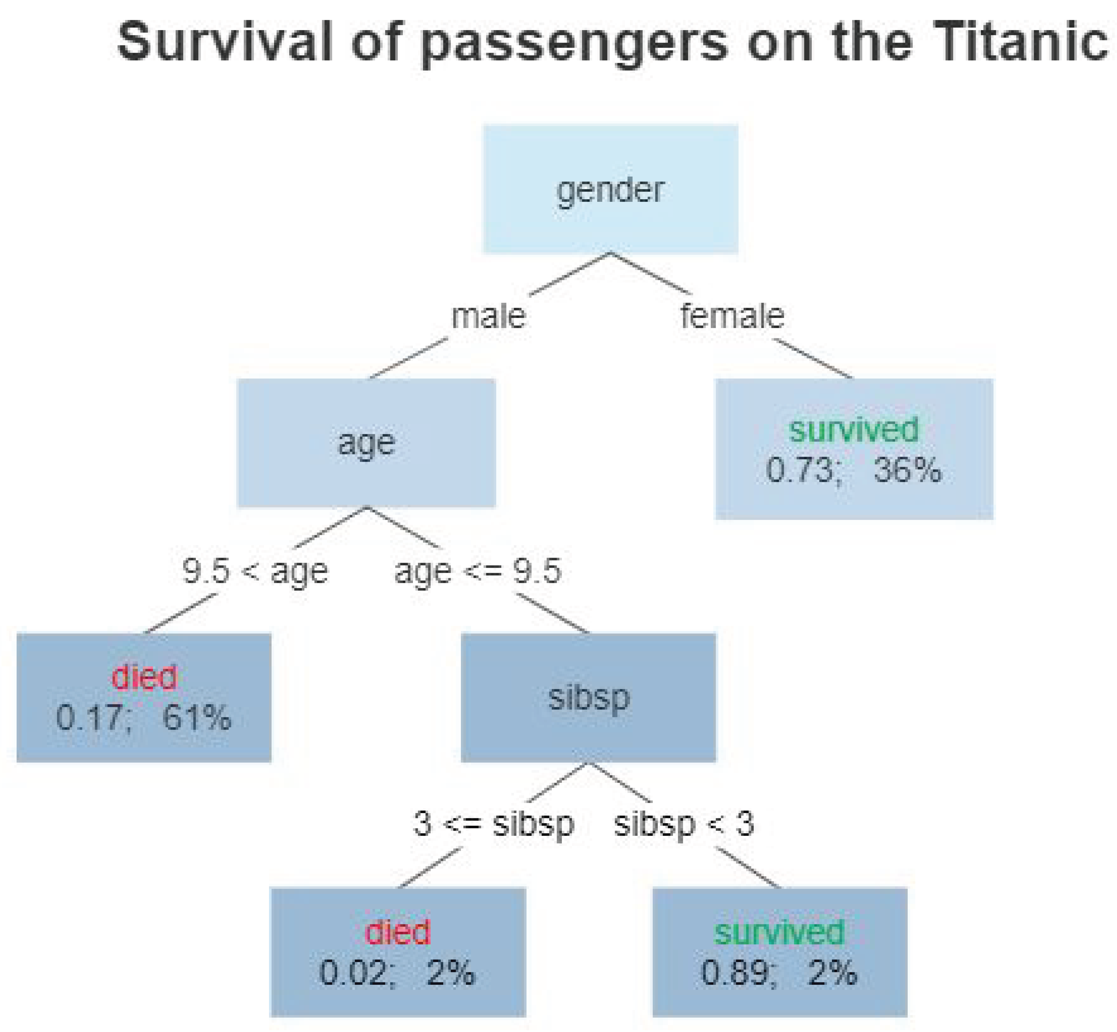
16.2.11.3 Mathematical Analysis of Decision Tree Learning
Decision tree learning is a fundamental supervised learning algorithm used for classification and regression tasks. It recursively partitions the feature space into distinct regions by selecting the most informative feature at each step based on a splitting criterion. The goal of a decision tree is to create a model that predicts the value of a target variable by learning simple decision rules inferred from data features. Given a dataset , where each is a feature vector and is the corresponding output (either categorical for classification or continuous for regression), a decision tree recursively partitions into disjoint regions , where each region corresponds to a leaf node containing a prediction for y. The function learned by the decision tree can be expressed as a piecewise constant function:
where M is the total number of leaf nodes, is the prediction assigned to region , and is an indicator function that is 1 if and 0 otherwise. The splitting criterion for a decision tree involves selecting the feature j and threshold s that best separate the data at each step. For classification, the impurity of a node is measured using a criterion such as the Gini impurity, defined as
where is the proportion of samples in region R belonging to class k, and K is the total number of classes. Another common impurity measure is entropy, given by
For regression, the variance reduction is typically used, and the impurity at a node is given by the mean squared error (MSE):
where is the mean of the target values in region R. The optimal split is found by maximizing the information gain, which is computed as
where and are the left and right child nodes obtained after splitting R, and is the impurity measure (Gini, entropy, or MSE). The algorithm selects the feature and threshold that maximize :
The recursive splitting process continues until a stopping criterion is met, such as a maximum depth D, a minimum number of samples per leaf , or an impurity threshold . The depth of the tree, denoted D, determines the complexity of the model, and the number of terminal nodes M satisfies
Pruning is performed to prevent overfitting, and one common approach is cost complexity pruning, which minimizes the function
where is a regularization parameter controlling the trade-off between tree complexity and accuracy. The optimal subtree is obtained by
Decision tree learning is computationally efficient, with a worst-case training complexity of
where N is the number of samples and d is the number of features. Despite its simplicity, decision trees can suffer from high variance, making ensemble methods such as random forests and gradient boosting necessary for improving generalization.
16.2.12. k-Nearest Neighbors Algorithm
16.2.12.1 Literature Review of k-Nearest Neighbors (KNN) Algorithm
Fix and Hodges (1951) [718] introduced the k-NN algorithm, laying the groundwork for non-parametric classification methods by proposing a technique where classification is based on the closest training examples in the feature space. Cover and Hart (1967) [719] provided a rigorous analysis of the k-NN algorithm’s properties, demonstrating that as the size of the dataset approaches infinity, the error rate of the k-NN classifier is at most twice the Bayes error rate, establishing its strong consistency. Devroye et. al. (2013) [720] offered an in-depth theoretical analysis of pattern recognition methods, including k-NN, and discusses their probabilistic properties and performance bounds. Toussaint (2005) [721] explored the use of geometric proximity graphs, such as Voronoi diagrams and Delaunay triangulations, to enhance the efficiency and accuracy of k-NN classifiers by structuring the data to reflect inherent geometric relationships. Arya et. al. (1998) [723] introduced an efficient algorithm for approximate nearest neighbor search, addressing the computational challenges of k-NN in high-dimensional spaces by allowing approximate solutions with provable bounds on their accuracy. Terrell and Scott (1992) [724] discussed variable kernel density estimation techniques, which are closely related to k-NN methods, providing insights into adaptive methods for density estimation that can improve k-NN performance in varying data densities. Samworth (2012) [725] investigated the weighting schemes in k-NN classifiers, proposing optimal weighting strategies that enhance classification performance, especially in situations where the assumption of uniformity in data distribution does not hold. Bremner et. al. (2005) [726] presented algorithms that compute the decision boundaries of k-NN classifiers more efficiently, making the application of k-NN more practical for large datasets by focusing computational efforts on the most critical regions of the feature space. Ramaswamy et. al. (2000) [727] introduced methods for detecting outliers using k-NN concepts, which are essential for identifying anomalies in large datasets and have applications in fraud detection, network security, and data cleaning. Cover (1999) [728] provided a comprehensive introduction to information theory, including discussions on k-NN and its connections to concepts such as entropy and mutual information, offering a theoretical foundation for understanding the behavior of k-NN in the context of information theory.
Table 37.
Summary of Contributions to k-nearest neighbors algorithm
| Reference | Key Contribution |
| Fix and Hodges (1951) | Introduced the k-NN algorithm as a non-parametric classification method, forming the foundation of instance-based learning. |
| Cover and Hart (1967) | Provided theoretical analysis proving that the k-NN error rate is at most twice the Bayes error, establishing its consistency. |
| Devroye, Györfi and Lugosi (1996) | Developed a probabilistic framework for pattern recognition, including bounds on k-NN performance. |
| Toussaint (2005) | Explored geometric proximity graphs to improve k-NN efficiency by structuring data spatially. |
| Arya et al. (1998) | Introduced an optimal approximate nearest neighbor search algorithm for high-dimensional spaces. |
| Terrell and Scott (1992) | Discussed variable kernel density estimation, offering insights into adaptive density-based k-NN improvements. |
| Samworth (2012) | Proposed optimal weighted k-NN classifiers, improving performance in non-uniform distributions. |
| Bremner et al. (2005) | Developed output-sensitive algorithms for computing k-NN decision boundaries efficiently. |
| Ramaswamy et al. (2000) | Applied k-NN for outlier detection in large datasets, aiding in anomaly detection applications. |
| Cover and Thomas (1991) | Connected k-NN to information theory concepts such as entropy and mutual information. |
16.2.12.2 Recent Literature Review of k-Nearest Neighbors (KNN) Algorithm
Alaca and Emin (2024) [729] evaluated KNN as part of hybrid models for medical kidney image classification. It compares KNN with Support Vector Machines (SVM) and Random Forest (RF), showcasing its strengths and weaknesses in medical image analysis. Chen et. al. (2025) [730] proposed a Probability-Integrated Projection (PIP)-based KNN algorithm for epidemic management, improving classification accuracy in medical datasets by optimizing distance metrics. Liu et. al. (2025) [731] used KNN for predicting bond strength in dental materials. The study demonstrates that KNN provides robust accuracy when combined with kernel-based methods like SVM. Barghouthi et. al. (2025) [732] introduced a multi-channel fusion approach using KNN for predicting pressure injuries in hospitalized patients, integrating KNN with deep learning models. Jewan (2025) [733] examined KNN’s effectiveness in remote sensing applications for crop yield prediction using UAV images, comparing it with Decision Trees and Random Forest. Moldovanu et. al. (2025) [734] studied how data corruption affects KNN’s accuracy, offering methods to improve KNN’s robustness using feature transformation. HosseinpourFardi and Alizadeh (2025) [735] proposed a hardware-accelerated KNN model for incremental learning, optimizing nearest-neighbor calculations in embedded systems. Afrin et. al. (2025) [736] used KNN to classify oil pipeline failure causes, demonstrating its reliability in industrial failure prediction. Hussain et. al. (2025) [737] evaluated KNN in geospatial flood susceptibility prediction, comparing it with RF and Extreme Gradient Boosting (XGBoost). Reddy and Murthy (2025) [738] combined Particle Swarm Optimization (PSO) with KNN to enhance accuracy in cardiovascular disease prediction.
Table 38.
Summary of Recent Contributions to k-nearest neighbors algorithm
| Author (Year) | Summary of Contributions |
| Alaca & Emin (2024) | Evaluates KNN within hybrid models for medical kidney image classification, comparing it with SVM and RF. Demonstrates how KNN performs in medical imaging tasks. |
| Chen, Hung & Yang (2025) | Proposes a Probability-Integrated Projection (PIP)-based KNN algorithm, improving classification accuracy for epidemic spread prediction through optimized distance metrics. |
| Liu et al. (2025) | Uses KNN for predicting bond strength of dental materials. Highlights KNN’s performance against kernel-based methods like SVM. |
| Barghouthi et al. (2025) | Develops a multi-channel fusion model using KNN for pressure injury prediction in hospitalized patients, integrating it with deep learning techniques. |
| Jewan (2025) | Examines KNN’s **effectiveness in remote sensing applications** for crop yield prediction using UAV images, comparing it with Decision Trees and RF. |
| Moldovanu et al. (2025) | Investigates how data corruption affects KNN’s accuracy, proposing feature transformation techniques to improve robustness. |
| HosseinpourFardi & Alizadeh (2025) | Introduces a hardware-accelerated KNN model for incremental learning, optimizing KNN’s performance in embedded systems. |
| Afrin et al. (2025) | Utilizes KNN to classify oil pipeline failure causes, demonstrating its effectiveness in industrial failure prediction. |
| Hussain et al. (2025) | Applies KNN to geospatial flood susceptibility prediction, comparing it with RF and XGBoost, showing its viability in disaster risk assessment. |
| Reddy & Murthy (2025) | Combines Particle Swarm Optimization (PSO) with KNN to enhance accuracy in cardiovascular disease prediction, demonstrating KNN’s adaptability in medical applications. |
Figure 180.
Framework of the k-nearest neighbors (KNN) algorithm. Image Credit: By Antti Ajanki AnAj - Own work, CC BY-SA 3.0, https://commons.wikimedia.org/w/index.php?curid=2170282. The green dot represents the test sample, which needs to be classified as either a blue square or a red triangle. If the classification is based on (solid-line circle), the sample is assigned to the red triangles because there are more triangles (2) than squares (1) within this region. However, with (dashed-line circle), the sample is classified as a blue square, as the outer circle contains three squares and only two triangles
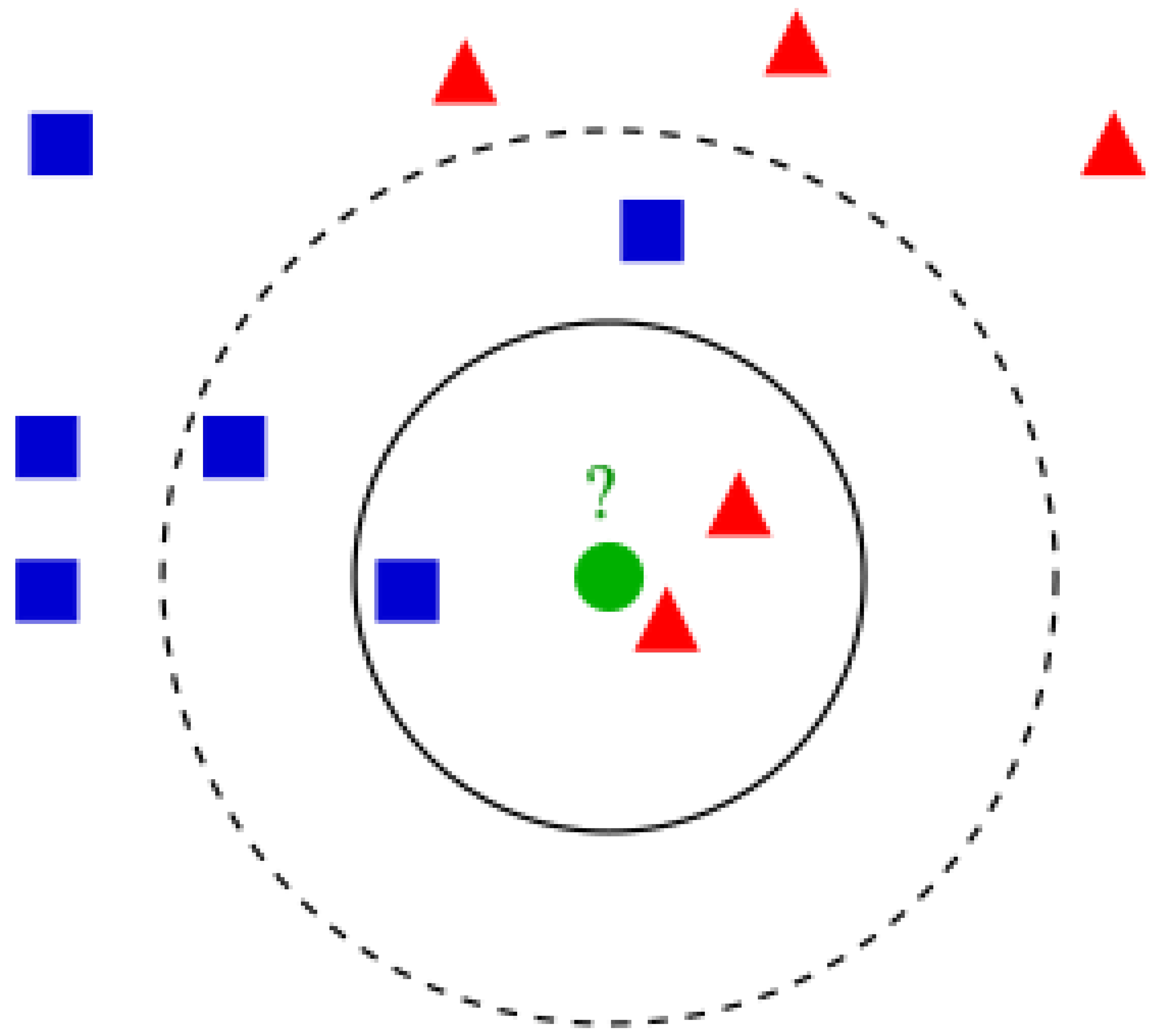
16.2.12.3 Mathematical Analysis of k-Nearest Neighbors (KNN) Algorithm
The k-nearest neighbors (KNN) algorithm is a fundamental instance-based learning method for classification and regression. It operates by determining the k nearest data points in the feature space and making predictions based on these neighbors. Formally, consider a dataset , where represents a d-dimensional feature vector, and represents the corresponding target variable. Given a new query point , the algorithm finds the k points in that are closest to under a chosen distance metric.
Mathematically, the distance function is commonly defined as the Euclidean distance:
Alternatively, the Minkowski distance of order p generalizes the Euclidean and Manhattan distances:
where corresponds to the Manhattan distance and corresponds to the Euclidean distance. For classification, the prediction is typically made using majority voting among the k nearest neighbors. Let be the set of indices of the k nearest neighbors of . The predicted class label is determined as:
where is the indicator function, and represents the set of all possible class labels. If weighted voting is used, the contribution of each neighbor can be weighted by the inverse distance:
where is a small positive number to prevent division by zero. The weighted class probability estimate is then given by:
and the final classification decision is:
For regression, the predicted value is typically the mean of the k nearest neighbors’ target values:
or, when distance weighting is applied,
Computational complexity is a critical aspect of KNN. A naive search for the nearest neighbors requires computing distances from to all N data points, leading to a time complexity of . If a spatial data structure such as a k-d tree or a ball tree is used, the query time can be reduced to in low-dimensional spaces. However, for high-dimensional data, the curse of dimensionality makes these structures less effective, often reverting to the brute-force complexity. The choice of k significantly affects KNN performance. A small k can lead to high variance, whereas a large k smooths the decision boundary but may introduce bias. The optimal k is often determined via cross-validation, where the classification error is minimized as:
The theoretical foundation of KNN can be analyzed in terms of consistency. Under mild assumptions, as and while , the KNN classification error converges to the Bayes error rate:
For regression, under similar asymptotic conditions, the expected squared error converges to:
In high-dimensional spaces, the effectiveness of KNN diminishes due to the concentration of distances:
The KNN decision boundary is a piecewise linear approximation of the true decision surface. In the limit as , KNN forms a Voronoi tessellation:
For , decision regions are obtained by aggregating Voronoi cells. Given a sample , the probability of class c is estimated as:
Thus, KNN is a flexible, non-parametric method that relies on local structure for decision-making.
16.2.13. Similarity Learning
16.2.13.1 Literature Review of Similarity Learning
Similarity training has evolved as a fundamental concept in machine learning, influencing areas such as classification, ranking, image retrieval, and natural language processing. The work of Chen et al. (2009) [739] provided a rigorous foundation for similarity-based classification by analyzing different approaches for converting similarities into kernel functions. Their study systematically explored the mathematical properties of similarity measures and their effect on classification performance, offering insights into optimal ways to utilize nearest neighbor weights. Chechik et al. (2010) [740] expanded upon this by introducing OASIS, an online learning algorithm designed to handle large-scale image similarity tasks efficiently. By leveraging a bilinear similarity function and optimizing with a large-margin criterion, OASIS achieved state-of-the-art performance in ranking tasks while maintaining computational feasibility. Similarly, Huang et al. (2013) [741] extended similarity learning into the domain of content-based image retrieval (CBIR) by integrating relative comparisons, an approach grounded in ranking theory. This refinement aligned image retrieval more closely with real-world applications, ensuring that retrieved images were ordered based on their true visual similarities rather than absolute feature distances.
The theoretical underpinnings of similarity-based learning were further explored by Kar and Jain (2011) [744], who proposed a framework for mapping similarity functions to data-driven embeddings. Their work addressed the crucial question of how similarity functions can be interpreted in terms of data separability, providing a bridge between metric learning and traditional feature-based classifiers. In a different but related direction, Xiao et al. (2011) [743] tackled the problem of positive and unlabeled learning (PU learning), where similarity functions were used to weight ambiguous examples and improve the classification of data points with uncertain labels. This approach demonstrated how similarity-based techniques could enhance learning in scenarios where labeled data is scarce or incomplete, making it particularly relevant for applications such as anomaly detection and biomedical classification.
With the advent of deep learning, similarity learning has expanded into more complex and high-dimensional data spaces. Yang et al. (2024) [742] conducted an extensive survey on deep learning approaches for similarity computation, covering applications ranging from sequence matching to graph-based similarity models. Their review provided a critical examination of various neural network architectures designed to capture similarity relationships in data, highlighting key challenges such as overfitting, interpretability, and computational efficiency. Additionally, contributions from Wikipedia contributors [746] have documented the broader theoretical framework of semantic similarity, including traditional node-based and edge-based methods for quantifying textual similarity. Co-citation proximity analysis, as explored in recent research, introduced an innovative way to determine document similarity by leveraging citation networks, demonstrating how similarity measures can be extended beyond direct content analysis to relational data structures.
From a practical implementation perspective, PingCAP (2024) [745] evaluated a range of tools for computing semantic similarity in natural language processing, including transformer-based models like BERT and classical vector representations such as Word2Vec. Their analysis underscored the trade-offs between model complexity, computational cost, and accuracy in different NLP applications. Finally, Choi (2022) [747] applied similarity scoring techniques to document retrieval and clustering, demonstrating how fine-grained textual similarity assessments can enhance information retrieval systems. By incorporating deep learning models, they showcased improvements in contextual understanding, making similarity-based approaches increasingly vital in modern AI applications. Collectively, these works highlight the evolution of similarity training, demonstrating its growing importance across disciplines while underscoring the interplay between theoretical advancements and real-world applications.
Table 39.
Summary of Contributions in Similarity Training
| Reference | Contribution |
| Chen et al. (2009) | Established a mathematical foundation for similarity-based classification by systematically converting similarity measures into kernels and evaluating their performance in various learning scenarios. |
| Chechik et al. (2010) | Developed OASIS, an efficient online algorithm that learns a bilinear similarity function for large-scale image ranking, optimizing a margin-based criterion to enhance ranking performance. |
| Wang et al. (2013) | Proposed a similarity learning framework for content-based image retrieval (CBIR) that incorporates relative comparisons, aligning retrieval results with human perception of image similarity. |
| Kar and Jain (2011) | Introduced a similarity embedding framework that maps similarity functions into data-driven feature spaces, bridging the gap between similarity learning and traditional classification approaches. |
| Liu et al. (2011) | Addressed positive and unlabeled (PU) learning by leveraging similarity-based weighting of uncertain examples, improving classification performance when labeled data is scarce. |
| Zhang et al. (2024) | Conducted an extensive survey on deep learning techniques for similarity learning, covering applications in sequence modeling, graph-based learning, and high-dimensional data similarity computation. |
| Wikipedia Contributors | Documented theoretical aspects of semantic similarity, including classical methods such as node-based and edge-based similarity computations, and their applications in knowledge representation. |
| PingCAP (2024) | Explored NLP tools like Word2Vec and BERT for semantic similarity computation, analyzing trade-offs between computational complexity and accuracy in various language processing applications. |
| ResearchGate Contributors (2023) | Demonstrated the application of similarity-based scoring techniques in document retrieval and clustering, showcasing improvements in contextual understanding using deep learning models. |
| Co-citation Proximity Analysis | Investigated citation-based similarity measures, introducing co-citation proximity analysis to quantify the relationship between academic articles based on their citation network structures. |
16.2.13.2 Recent Literature Review of Similarity Learning
Nanyonga et. al. (2025) [707] presented a transformer-based approach for predicting causes of aviation incidents using similarity training. It introduces a multi-head attention mechanism that evaluates patterns in historical incident data to improve predictive accuracy. The model achieves a similarity score of 0.697 with a standard deviation of ±0.153, highlighting the effectiveness of the similarity training approach. Fan and Chung (2025) [708] leveraged similarity-based training to classify crops in UAV-captured images. It employs RGB and vegetation indices (VARI) for training, optimizing performance by balancing training and testing datasets with an 80/20 split. The model improves classification accuracy by using similarity metrics to refine feature extraction. Bakaev et. al. (2025) [709] explored similarity-based training methods to enhance synthetic text generation by Large Language Models (LLMs). Using cosine similarity and Mahalanobis distance, the authors analyze how closely generated text matches human-authored content, showcasing the effectiveness of similarity-based methods in controlling model outputs. Ahn et. al. (2025) [711] employed similarity training using the Dice Similarity Coefficient to fine-tune a deep learning model for medical image segmentation. The proposed method significantly improves precision in identifying standard imaging planes, demonstrating how similarity metrics enhance training effectiveness. Peng et. al. (2025) [712] introduced similarity label supervision to refine visual place recognition by improving re-ranking mechanisms. By integrating descriptor similarity into the training process, the model enhances recognition performance even in challenging environmental conditions. Zhao et. al. (2025) [713] employed similarity-based global distance measures to cluster data while preserving privacy in federated learning. The authors integrate Generative Adversarial Networks (GANs) to refine the training process, ensuring robust clustering in distributed environments. Wang et. al. (2025) [714] developed a similarity matrix (W matrix) to predict genomic traits in maize hybrids. By incorporating similarity measures into training, the model improves yield and moisture content predictions across different environmental conditions. Xu et. al. (2025) [715] introduced a similarity loss function in medical image registration. By optimizing image similarity during training, the authors achieve enhanced alignment accuracy for medical imaging applications. Sun et. al. (2025) [716] investigated how similarity training affects text generation in LLMs. It evaluates ROUGE-1 similarity scores to measure how synthetic text diverges from human-generated content, guiding training strategies for better alignment with human language patterns. Liang et. al. (2025) [717] presented a similarity-based training approach to improve lip-to-speech synthesis. The model learns to generate natural-sounding speech without explicit speaker embeddings, achieving high speaker similarity through deep learning methods.
Table 40.
Summary of Recent Contributions in Similarity Training
| Reference | Title | Contribution |
| Nanyonga et al. (2025) | Multi-Head Attention-Based Transformer Model for Predicting Causes in Aviation Incidents | Introduces a transformer-based similarity training approach to predict aviation incidents with a multi-head attention mechanism, achieving a similarity score of 0.697. |
| Fan & Chung (2025) | Integrating Image Processing Technology and Deep Learning to Identify Crops in UAV Orthoimages | Uses similarity training to classify crops in UAV images, leveraging RGB and vegetation indices (VARI) to improve accuracy. |
| Bakaev et al. (2025) | Who Will Author the Synthetic Texts? | Implements cosine similarity and Mahalanobis distance for evaluating synthetic text similarity, improving text coherence in LLMs. |
| Ahn et al. (2025) | Deep Learning-Based Automated Guide for Developmental Dysplasia of the Hip Screening | Employs the Dice Similarity Coefficient to optimize deep learning-based segmentation in medical imaging. |
| Peng et al. (2025) | Range and Bird’s Eye View Fused Cross-Modal Visual Place Recognition | Introduces similarity label supervision to refine visual place recognition through descriptor similarity search. |
| Zhao et al. (2025) | Privacy-Preserved Federated Clustering with Non-IID Data via GANs | Uses similarity-based clustering and GANs to enhance privacy-preserved federated learning. |
| Wang et al. (2025) | Accurate Genomic Prediction for Maize Hybrids Using Multi-Environment Data | Develops a similarity matrix (W matrix) for genomic prediction, improving maize yield and moisture content predictions. |
| Xu et al. (2025) | Medical Image Registration Meets Vision Foundation Model: Prototype Learning and Contour Awareness | Introduces similarity loss functions to optimize image registration in medical imaging applications. |
| Sun et al. (2025) | Idiosyncrasies in Large Language Models | Evaluates similarity training effects on LLM-generated text, analyzing divergence from human-authored content using ROUGE-1 similarity scores. |
| Liang et al. (2025) | NaturalL2S: High-Quality Multi-Speaker Lip-to-Speech Synthesis | Employs similarity-based training to enhance lip-to-speech synthesis, achieving high speaker similarity. |
Figure 181.
Autoencoder architecture. Image Credit: https://developers.google.com/machine-learning/clustering/dnn-clustering/overview
Figure 181.
Autoencoder architecture. Image Credit: https://developers.google.com/machine-learning/clustering/dnn-clustering/overview
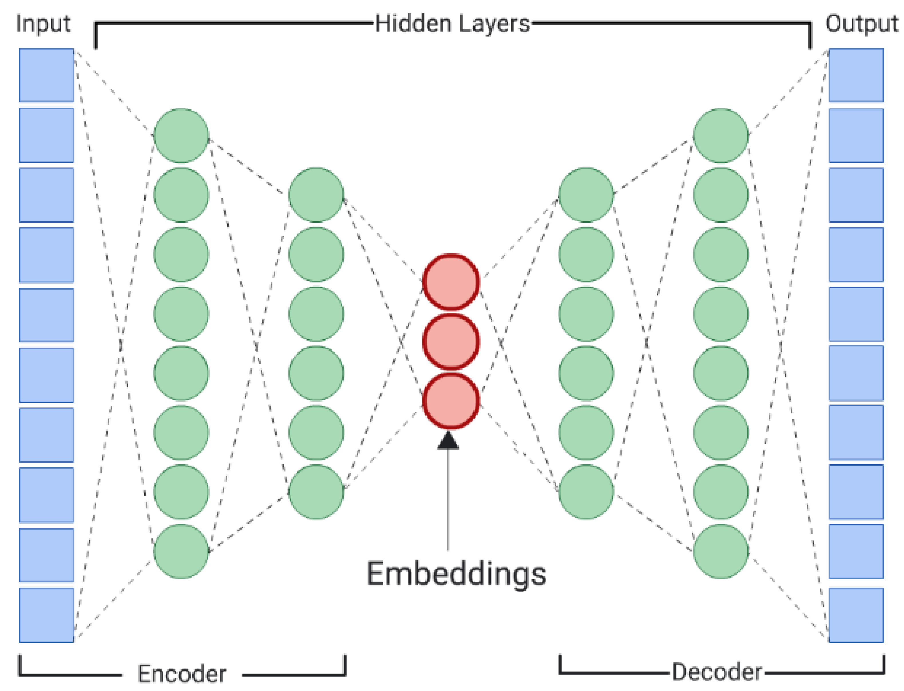
Figure 182.
Predictor architecture. Image Credit: https://developers.google.com/machine-learning/clustering/dnn-clustering/overview
Figure 182.
Predictor architecture. Image Credit: https://developers.google.com/machine-learning/clustering/dnn-clustering/overview
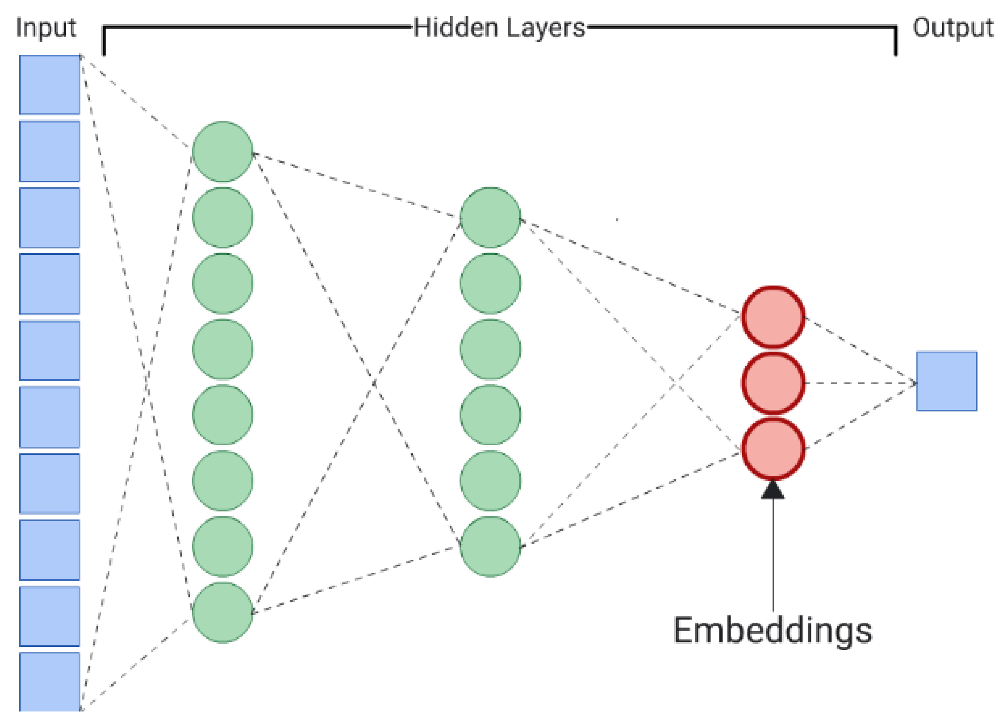
16.2.13.3 Mathematical Analysis of Similarity Learning
Similarity learning is a fundamental paradigm in machine learning and mathematical optimization that focuses on learning a function that maps inputs to a representation space where similar inputs are placed closer together, while dissimilar inputs are pushed farther apart. Mathematically, given a dataset , where are feature vectors and is a similarity label (where indicates similarity and indicates dissimilarity), similarity learning aims to learn a function such that a distance metric satisfies
for some threshold . A common choice for D is the Euclidean distance,
A central approach in similarity learning is metric learning, where the goal is to learn a distance metric M that parameterizes a Mahalanobis-like distance
where M is a positive semi-definite (PSD) matrix (), ensuring that satisfies the properties of a metric:
Metric learning can be formulated as an optimization problem where we minimize a loss function that enforces similarity constraints. One such loss function is the contrastive loss
where is a margin parameter. This loss ensures that similar samples are pulled together while dissimilar samples are pushed apart beyond a margin. Another widely used loss function is the triplet loss, which operates on triplets , where is an anchor, is a positive example, and is a negative example. The triplet loss is defined as
Here, the objective is to ensure that the distance between the anchor and the positive is smaller than the distance between the anchor and the negative by at least a margin . If we represent the embedding function as a deep neural network parameterized by , then similarity learning becomes a deep learning problem, where the network parameters are optimized via stochastic gradient descent to minimize one of the loss functions described above. A particularly effective approach in similarity learning is the use of a Siamese network, where two identical neural networks share weights and process two input vectors and . The network learns a representation such that the Euclidean distance
is small for similar pairs and large for dissimilar pairs. The optimization is driven by minimizing a loss function such as the contrastive or triplet loss. Another approach is the use of graph-based similarity learning, where a similarity graph is constructed over the dataset, and embeddings are learned by enforcing that connected nodes are closer together in the embedding space. This can be formulated as
where is a weight representing the strength of similarity between and . Thus, similarity learning encompasses a vast array of methods, from classical metric learning with Mahalanobis distances to deep learning approaches with Siamese networks, triplet loss, and self-supervised contrastive learning, all of which fundamentally rely on defining and optimizing a notion of similarity in a mathematically rigorous manner.
16.3. Self Learning
16.3.1. Literature Review of Self Learning
Self-learning in artificial intelligence has evolved through various paradigms, including reinforcement learning, self-supervised learning, meta-learning, and curiosity-driven exploration. A foundational work in this domain is Schmidhuber’s (1991) [123] research on curiosity-driven model-building, which introduced the concept of intrinsic motivation in learning systems. He proposed that an agent should actively seek novel experiences by maximizing learning progress, thereby enhancing its predictive capabilities. This principle has been extensively applied in reinforcement learning (RL) to encourage efficient exploration in complex environments, forming the basis of modern exploration bonuses used in deep RL. Reinforcement learning itself was rigorously formalized by Sutton (2018) [286] and Barto (2021) [287], who introduced the Markov Decision Process (MDP) framework and core algorithms like temporal difference (TD) learning and actor-critic architectures. Their work established self-learning via trial-and-error, wherein an agent refines its policy through rewards and penalties, ultimately enabling autonomous decision-making without explicit supervision. Building upon these foundations, Silver et al. (2017) [851] demonstrated how self-play in AlphaZero allows an agent to master games like chess, shogi, and Go without human data, utilizing deep RL with Monte Carlo Tree Search (MCTS) to iteratively refine strategies through self-competition.
Beyond reinforcement-based methods, self-supervised learning (SSL) has emerged as a crucial paradigm for learning without labeled data. Bengio et al. (2009) [283] introduced curriculum learning, which simulates the human cognitive process by training models on simpler tasks before progressing to complex ones. This approach has been shown to significantly improve convergence rates and generalization in deep learning. He et al. (2020) [852] further advanced SSL through contrastive learning, where Momentum Contrast (MoCo) enables a model to differentiate instances based on learned feature representations, even in the absence of labels. Grill et al. (2020) [853] introduced Bootstrap Your Own Latent (BYOL), a breakthrough demonstrating that self-learning representations do not require negative pairs (a key contrastive learning element). Instead, BYOL employs an online and target network paradigm to iteratively refine embeddings, proving that deep neural networks can self-learn meaningful features without explicit contrastive mechanisms. This non-contrastive learning methodology has been a significant step toward fully autonomous feature extraction, eliminating the need for carefully curated negative samples in self-learning tasks.
In the context of hierarchical self-learning, Hinton et al. (2006) [854] proposed Deep Belief Networks (DBNs), pioneering layer-wise unsupervised pretraining, which allows deep networks to learn robust feature hierarchies. This method was pivotal in self-learning hierarchical representations and directly influenced architectures like autoencoders, GANs, and modern deep networks. Similarly, meta-learning, or “learning how to learn,” was formalized by Finn et al. (2017) [855] through Model-Agnostic Meta-Learning (MAML). Their framework demonstrated that deep networks could be optimized to rapidly adapt to new tasks using only a few gradient steps, showcasing self-learning’s potential in few-shot learning and robotics. Additionally, Jaderberg et al. (2017) [856] introduced auxiliary self-learning objectives in RL, where an agent trains on unsupervised auxiliary tasks, such as predicting future states, to enhance representation learning and sample efficiency. This method demonstrated that reinforcement learning agents could self-discover useful intermediate goals, thereby accelerating policy convergence and improving generalization across multiple tasks.
Finally, the transformer revolution has brought self-learning capabilities to vision tasks, as demonstrated by Dosovitskiy et al. (2020) [857] with Vision Transformers (ViTs). They showed that self-attention mechanisms—originally developed for natural language processing—could replace convolutional architectures, allowing deep networks to self-learn image representations without handcrafted priors. This introduced a paradigm shift where models no longer rely on spatial inductive biases, instead learning global dependencies in a self-supervised manner. Collectively, these contributions have rigorously established self-learning as a fundamental principle in artificial intelligence, spanning multiple disciplines and application areas. From curiosity-driven exploration and reinforcement-based self-play to self-supervised feature learning and meta-learning, self-learning methodologies now underpin state-of-the-art AI systems, enabling them to autonomously acquire knowledge, optimize representations, and generalize across domains with minimal or no human intervention.
Table 41.
Summary of Contributions in Self-Learning
| Reference | Contribution |
| Schmidhuber (1991) | Introduced curiosity-driven learning and intrinsic motivation for self-learning agents. |
| Sutton and Barto (1998) | Formalized reinforcement learning through MDPs, TD learning, and actor-critic architectures. |
| Silver et al. (2017) | Demonstrated self-play in AlphaZero, mastering games without human input using MCTS. |
| Bengio et al. (2009) | Introduced curriculum learning, simulating human cognitive progression in deep learning. |
| He et al. (2020) | Developed contrastive learning through Momentum Contrast (MoCo) for self-supervised learning. |
| Grill et al. (2020) | Introduced BYOL, proving self-supervised learning without negative pairs. |
| Hinton et al. (2006) | Pioneered deep belief networks (DBNs) for hierarchical self-learning representations. |
| Finn et al. (2017) | Formalized model-agnostic meta-learning (MAML) for few-shot learning. |
| Jaderberg et al. (2017) | Proposed auxiliary self-learning objectives in RL to enhance policy learning. |
| Dosovitskiy et al. (2020) | Developed Vision Transformers (ViTs), enabling self-learning representations in vision tasks. |
16.3.2. Recent Literature Review of Self Learning
Self-learning artificial intelligence (AI) has made significant advances across diverse domains, including ethical considerations, scientific research, healthcare, and education. The first major contribution is from Mousavi (2025) [858], who explores the ethical implications of self-aware AGI, questioning whether such AI systems should be granted moral consideration akin to conscious beings. This work utilizes fuzzy logic to determine whether AI self-awareness equates to possessing a "soul," raising crucial debates about data deletion, AI rights, and governance. Similarly, Cui et al. (2025) [860] propose a dual-level self-supervised learning framework to enhance the generalization capabilities of AI in interatomic potential modeling. By improving AI’s ability to adapt to out-of-distribution data, their work has a profound impact on computational chemistry and materials science. Meanwhile, Jia et al. (2025) [861] apply self-supervised graph learning techniques to molecular property prediction. Their research focuses on fragment-level feature fusion, using retrosynthetic fragmentation algorithms to improve drug discovery by learning molecular representations without labeled data. These studies highlight the expanding role of self-learning AI in scientific and ethical discussions.
In healthcare and medical applications, self-learning AI continues to demonstrate transformative capabilities. Liu et al. (2025) [863] introduce a self-optimized reinforcement learning algorithm for elective surgery scheduling, significantly enhancing hospital efficiency by dynamically optimizing multi-specialty, multi-stage procedures. Additionally, Song et al. (2025) [864] develop a deep self-supervised learning framework for time series classification, optimizing AI’s ability to detect anomalies in various domains, including finance and industrial monitoring. In another critical medical application, Chaudary et al. (2025) [870] design an EEG-based emotion recognition system utilizing explainable AI. Their model interprets neural activity patterns to enhance human-computer interaction, which is vital for mental health monitoring and affective computing. Expanding further into neuroscience, Tautan et al. (2025) [871] present a systematic review of unsupervised learning methods applied to epilepsy detection using EEG data. Their work highlights AI’s ability to classify seizures with minimal human intervention, improving diagnostic accuracy and reducing the burden on neurologists. These contributions showcase AI’s ability to autonomously learn from complex biomedical signals, paving the way for intelligent decision-making in healthcare.
The role of self-learning AI extends beyond the medical field into education and cognitive sciences. Hou (2025) [862] investigates the integration of AI-supported learning environments with students’ psychological factors such as self-esteem and mindfulness. Their findings suggest that AI-driven adaptive learning platforms foster personalized education, optimizing student performance through tailored feedback mechanisms. A related study by Li et al. (2025) [869] explored generative AI’s role in real-time adaptive scaffolding for self-regulated learning. By analyzing student behaviors in real time, AI dynamically generates learning resources that adapt to individual needs, significantly enhancing personalized education strategies. Furthermore, Bjerregaard et al. (2025) [859] examine how self-supervised learning can be applied to structural biology, particularly in protein folding studies. Their research provides a foundation for AI-driven drug discovery and molecular engineering by leveraging AI models that can learn protein structures from vast amounts of unlabeled data. These studies highlight the increasing influence of self-learning AI in shaping education, scientific research, and personalized cognitive support.
Across these domains, self-learning AI is emerging as a revolutionary tool capable of independently acquiring knowledge, recognizing patterns, and making informed decisions without human intervention. Its impact ranges from ethical AI governance to improving biomedical diagnostics, optimizing industrial and financial systems, and reshaping education. The convergence of self-learning AI with reinforcement learning, self-supervised learning, and generative AI models demonstrates its versatility in tackling real-world challenges. By continuously refining its ability to learn from limited data, detect anomalies, and optimize decision-making, self-learning AI is poised to drive future innovations in science, healthcare, and education. These rigorous contributions underscore the growing necessity of developing AI systems that not only automate tasks but also refine their understanding of complex environments, leading to more autonomous and intelligent machines.
Table 42.
Summary of Recent Contributions in Self-Learning
| Paper | Contribution |
| Mousavi (2025) | Examines the ethical implications of self-aware AGI and whether it possesses moral standing. Utilizes fuzzy logic to assess AI consciousness, influencing AI governance debates. |
| Bjerregaard et al. (2025) | Demonstrates the application of self-supervised learning to structural biology, improving molecular structure prediction and advancing computational drug discovery. |
| Cui et al. (2025) | Develops a dual-level self-supervised learning model to enhance generalization in physics-based AI, particularly in interatomic potential modeling. |
| Jia et al. (2025) | Introduces a graph-based self-supervised learning model for molecular property prediction, utilizing retrosynthetic fragmentation to improve AI-driven drug design. |
| Hou (2025) | Investigates the psychological effects of AI-driven adaptive learning on self-esteem and academic mindfulness, highlighting AI’s role in personalized education. |
| Liu et al. (2025) | Proposes a reinforcement learning-based scheduling system for elective surgeries, optimizing hospital efficiency and reducing patient wait times. |
| Song et al. (2025) | Develops a deep self-supervised learning framework for anomaly detection in time-series data, improving AI applications in finance and industry. |
| Li et al. (2025) | Explores generative AI’s ability to provide real-time adaptive scaffolding for personalized self-regulated learning, enhancing online education strategies. |
| Chaudary et al. (2025) | Presents an EEG-based AI model for emotion recognition using self-learning algorithms, improving human-computer interaction and mental health monitoring. |
| Tautan et al. (2025) | Conducts a systematic review of unsupervised learning methods for epilepsy detection using EEG data, showcasing AI’s diagnostic potential in neurology. |
16.3.3. Mathematical Analysis of Self Learning
Self-learning is a process by which an entity, be it biological or artificial, acquires knowledge, refines understanding, and adapts behavior without direct external instruction. Mathematically, self-learning can be framed in the context of optimization, function approximation, and iterative improvement of hypotheses, drawing upon formalism from information theory, machine learning, and dynamical systems. Given an unknown target function , self-learning aims to construct an approximation such that
in some well-defined sense, typically minimizing an objective function over an appropriate hypothesis space . If we let denote inputs and denote corresponding outputs, then a fundamental formulation of self-learning can be described as an empirical risk minimization (ERM) problem:
where L is a loss function that quantifies the discrepancy between the actual outcome and the predicted outcome .
In an idealized self-learning system, the function evolves dynamically as additional information is acquired, which can be described by an update rule:
where is a learning rate and denotes the gradient of the loss function with respect to the model parameters. A crucial aspect of self-learning is the incorporation of feedback mechanisms, whereby an entity refines its internal model based on past errors. This can be framed in terms of stochastic gradient descent (SGD):
where represents the parameters of the function approximator . If the system has access to reinforcement signals rather than explicit input-output pairs, self-learning aligns with reinforcement learning, where the goal is to maximize an expected cumulative reward:
where is a policy mapping states to actions, is a reward function, and is a discount factor. The optimal policy satisfies the Bellman equation:
which recursively expresses the expected return of a state-action pair. In an unsupervised setting, self-learning often manifests through clustering or density estimation, where the objective is to model the underlying distribution . One way to formalize this is through maximum likelihood estimation:
which seeks to find model parameters that best explain the observed data. A more flexible formulation involves variational inference, where we approximate the posterior distribution using a tractable function and minimize the Kullback-Leibler (KL) divergence:
which ensures that is close to the true posterior . Self-learning in neural systems can be framed using Hebbian learning principles, where synaptic weights evolve according to activity correlations:
or more generally through spike-timing-dependent plasticity (STDP):
where represents the temporal offset between presynaptic and postsynaptic activations. In deep learning, self-learning often involves self-supervised contrastive learning, which optimizes an objective of the form:
where is a positive sample, represents negative samples, and measures similarity in representation space. This encourages self-learned representations to be invariant under transformations. Mathematically, self-learning is deeply connected to information-theoretic principles, particularly in maximizing the mutual information between learned representations Z and the data X:
which captures the reduction in uncertainty about Z given knowledge of X. A self-learning system thus seeks to construct representations that maximize while discarding task-irrelevant noise. More generally, if self-learning operates within a Bayesian framework, it continuously updates a posterior belief over hypotheses using Bayes’ theorem:
where D represents the accumulated data. Finally, in the context of dynamical systems, self-learning can be modeled as a time-dependent process governed by differential equations, such as the Riccati equation in adaptive control:
where P represents a learning-induced adaptation of system dynamics. Self-learning is thus an iterative, evolving process that refines internal models through optimization, probabilistic inference, feedback-driven adaptation, and information maximization.
16.3.4. Python Code to Generate Figure 183
The Python code below produces the Figure 183 illustrating the Self-Learning.
Figure 183.
Decision boundary of a Self-Learning (Self-Training) classifier. The classifier is initially trained on labeled data, predicts labels on unlabeled data, and iteratively updates itself using confident predictions. The contour regions represent predicted classes, and scatter points show the original data points
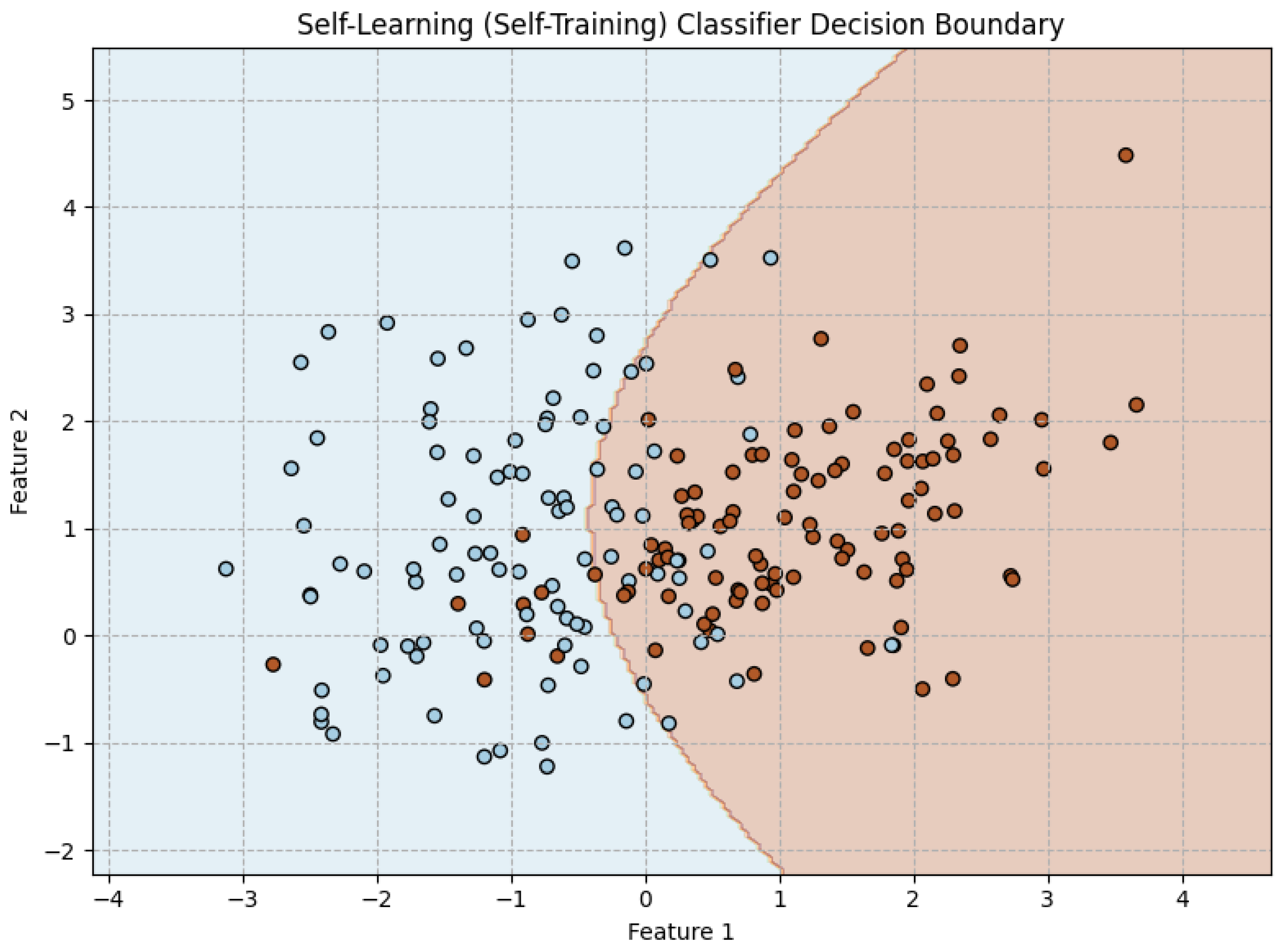
16.4. Reinforcement Learning
16.4.1. Literature Review of Reinforcement Learning
Reinforcement Learning (RL) has evolved from fundamental theoretical concepts to sophisticated algorithms capable of solving high-dimensional decision-making problems. The foundational work by Bellman (1954) [891] introduced Dynamic Programming (DP), establishing the Bellman equations that recursively compute optimal value functions in Markov Decision Processes (MDPs). This formulation became the mathematical backbone for reinforcement learning, particularly in value iteration and policy iteration methods. Decades later, Sutton and Barto (1998, 2018) [286] [287] formalized RL as a computational framework for sequential decision-making, introducing core concepts such as temporal difference (TD) learning, policy evaluation, and actor-critic architectures. Their seminal book remains the primary reference for both theoretical research and practical applications, covering both classical algorithms like Q-learning (Watkins and Dayan, 1992) [893] and deep reinforcement learning techniques. The work of Watkins and Dayan (1992) [893] is particularly crucial, as it introduced Q-learning, a model-free off-policy RL algorithm that enables an agent to learn an optimal policy without requiring an explicit model of the environment. The proof of convergence of Q-learning under certain conditions laid the foundation for later deep RL algorithms such as Deep Q Networks (DQN).
A major milestone in RL came with Mnih et al. (2015) [292], who introduced Deep Q Networks (DQN), combining deep neural networks with Q-learning to solve high-dimensional control problems. Their method incorporated experience replay to break correlation in training data and target networks for stable Q-value updates, allowing for the first superhuman performance on Atari games using raw pixel inputs. The introduction of deep RL opened the door to applications in robotics, game AI, and autonomous systems. The subsequent work of Silver et al. (2016) [892] extended deep RL into combinatorial search problems, with AlphaGo integrating Monte Carlo Tree Search (MCTS) with deep policy and value networks. This demonstrated the potential of RL in solving long-horizon planning problems and led to AlphaZero, which generalizes the method to various board games, achieving superhuman performance in Go, chess, and shogi without human supervision. Parallel to these advances, Konda and Tsitsiklis (2000) [293] introduced actor-critic algorithms, which separate the value function estimator (critic) from the policy update mechanism (actor), leading to more stable policy learning. This framework influenced modern policy optimization techniques such as Proximal Policy Optimization (PPO), developed by Schulman et al. (2017) [894], which uses a clipped surrogate objective to ensure stable updates without excessive deviation from the current policy.
In the realm of continuous control, Lillicrap et al. (2016) [895] introduced Deep Deterministic Policy Gradient (DDPG), an off-policy actor-critic method that enables RL in high-dimensional continuous action spaces. Unlike DQN, which operates in discrete action spaces, DDPG employs a deterministic policy with target networks and batch normalization for stable learning. Building on these ideas, Haarnoja et al. (2018) [291] proposed Soft Actor-Critic (SAC), incorporating entropy maximization to encourage exploration and improve sample efficiency. SAC’s stochastic policy formulation and automatic entropy adjustment mechanism set a new standard for continuous control tasks in RL. Meanwhile, Levine et al. (2016) [294] demonstrated the feasibility of end-to-end learning for robotics, directly mapping visual inputs to control actions using deep reinforcement learning. Their guided policy search method combined RL with supervised learning to improve sample efficiency, paving the way for RL-based autonomous robotic systems. These collective advancements, spanning from fundamental RL principles to modern deep learning integration, have established reinforcement learning as a powerful tool for solving complex decision-making and control problems in diverse applications.
Table 43.
Summary of Key Contributions in Reinforcement Learning
| Reference | Contribution |
| Bellman (1957) | Introduced Dynamic Programming, laying the mathematical foundation for reinforcement learning. Developed the Bellman equation, which enables recursive computation of optimal policies in Markov Decision Processes (MDPs). |
| Sutton and Barto (1998, 2018) | Formalized reinforcement learning as a computational framework. Introduced key concepts such as temporal difference (TD) learning, actor-critic methods, and policy evaluation. Their textbook serves as the primary resource for both theoretical and applied RL. |
| Watkins and Dayan (1992) | Developed Q-learning, a model-free off-policy algorithm that enables agents to learn optimal policies without requiring an explicit model of the environment. Provided proof of Q-learning’s convergence under certain conditions. |
| Mnih et al. (2015) | Introduced Deep Q Networks (DQN), combining deep learning with Q-learning to handle high-dimensional state spaces. Innovations include experience replay and target networks, leading to stable and sample-efficient training. Achieved superhuman performance on Atari games. |
| Silver et al. (2016) | Developed AlphaGo, which integrated Monte Carlo Tree Search (MCTS) with deep reinforcement learning. Demonstrated the ability to learn complex planning tasks with deep policy and value networks. Paved the way for AlphaZero, which generalized the approach to chess and shogi. |
| Konda and Tsitsiklis (2000) | Proposed actor-critic methods, separating policy learning (actor) from value estimation (critic). Their framework improved policy stability and inspired modern policy gradient methods such as Proximal Policy Optimization (PPO). |
| Schulman et al. (2017) | Developed Proximal Policy Optimization (PPO), a policy gradient method using a clipped objective function to stabilize training. PPO is widely used due to its balance between sample efficiency and simplicity. |
| Lillicrap et al. (2016) | Introduced Deep Deterministic Policy Gradient (DDPG), extending reinforcement learning to continuous action spaces. Utilized deterministic policies, target networks, and batch normalization to improve stability. |
| Haarnoja et al. (2018) | Developed Soft Actor-Critic (SAC), which incorporates entropy maximization for improved exploration and stability. SAC’s stochastic policy formulation and automatic entropy adjustment enhanced sample efficiency. |
| Levine et al. (2016) | Applied reinforcement learning to robotics using guided policy search. Combined RL with supervised learning to improve sample efficiency, demonstrating end-to-end learning from raw sensory inputs to control outputs. |
16.4.2. Recent Literature Review of Reinforcement Learning
Reinforcement Learning (RL) has seen substantial advancements in recent research, spanning diverse applications from security and AI planning to industrial systems and environmental monitoring. A key development in RL is its application to cybersecurity, as highlighted by Shah’s (2025) [896] research on adversarial vulnerabilities in RL models. This study systematically investigates how RL-based AI systems can be compromised through adversarial attacks and proposes mitigation strategies to enhance robustness. This security-oriented approach is complemented by Ajanovi et al. (2025) [897], who bridge the gap between AI planning and RL by integrating structured planning methods with reinforcement learning to create interpretable and reliable decision-making frameworks. Their work addresses a long-standing challenge in AI: ensuring that RL-based decision models remain understandable and controllable, a crucial aspect in mission-critical applications. Similarly, Oliveira et al. (2025) [898] introduce spatial cluster detection using RL, revolutionizing geospatial analysis by allowing RL models to identify non-regular spatial clusters, which traditional statistical techniques struggle to detect.
Beyond planning and security, RL is making strides in multi-agent decision-making systems. Hengzhi et al. (2025) [899] leverage multi-agent reinforcement learning (MARL) for UAV relay covert communication, optimizing real-time transmission strategies for secure aerial data networks. This work highlights the potential of RL in decentralized, high-stakes environments where autonomous agents must coordinate under uncertainty. The concept of multi-task learning is further expanded by Pan et al. (2025) [900], who propose a Markov Decision Process (MDP)-based task grouping approach that enables RL models to learn multiple tasks efficiently. This innovation addresses a fundamental limitation of RL: its need for extensive task-specific training, making it more scalable across diverse problem domains. Similarly, Liu et al. (2025) [901] explore multi-hop knowledge graph reasoning, applying RL to enhance automated reasoning processes in knowledge systems, significantly improving the efficiency of complex decision chains.
RL is also proving instrumental in energy and infrastructure resilience. Chen et al. (2025) [902] propose an interpretable RL framework for building energy management, ensuring that deep RL models remain transparent while optimizing energy consumption in smart building systems. Their work addresses a key limitation of black-box AI models by extracting human-readable decision rules, bridging the gap between efficiency and interpretability. Anwar and Akber (2025) [903] extend RL applications to structural resilience, using multi-agent deep RL to enhance the durability of buildings under extreme environmental conditions. This work is pivotal in modern urban planning, demonstrating how RL can optimize interconnected physical infrastructures for enhanced resilience. Zhao et al. (2025) [904] apply RL-enhanced long short-term memory (LSTM) networks to predictive maintenance, improving industrial fault detection by optimizing data-driven health assessments of rolling bearings. By integrating RL with deep learning models, they achieve superior early fault detection, reducing operational risks in industrial automation.
Finally, RL is shaping mental health support and empathetic AI. Soman et al. (2025) [905] introduce reinforcement learning-enhanced retrieval-augmented generation (RAG) models for mental health AI agents, where RL fine-tunes AI-generated responses to provide more personalized and empathetic support. This integration is crucial in human-AI interactions, ensuring that mental health support systems align with human emotional needs. Overall, these studies collectively demonstrate the growing versatility of reinforcement learning across disciplines, tackling challenges in security, multi-agent coordination, AI transparency, and intelligent automation. As RL techniques continue to evolve, they are poised to redefine decision-making, infrastructure resilience, and human-centric AI interactions in unprecedented ways.
Table 44.
Summary of Key Contributions in Recent Reinforcement Learning
| Authors, Year, and Source | Key Contribution |
| H. Shah (2025), ResearchGate | Explores the security vulnerabilities of reinforcement learning (RL) models to adversarial attacks and proposes mitigation techniques for model robustness. |
| B. Hengzhi, W. Haichao, H. Rongrong, et al. (2025), Chinese Journal of Aeronautics (Elsevier) | Uses multi-agent reinforcement learning (MARL) to optimize UAV relay covert communication, improving security and efficiency in real-time transmission. |
| R. Pan, Q. Yuan, G. Luo, B. Chen, et al. (2025), SSRN | Introduces a novel Markov Decision Process (MDP) graph-based approach to improve sample efficiency in multi-task reinforcement learning (MTRL). |
| G. Soman, M.V. Judy, A.M. Abou (2025), Cognitive Systems Research (Elsevier) | Applies reinforcement learning to enhance Retrieval-Augmented Generation (RAG) for AI-driven mental health support systems. |
| D.R.X. Oliveira, G.J.P. Moreira, A.R. Duarte (2025), Environmental and Ecological Statistics (Springer) | Develops RL-based spatial cluster detection techniques to improve geospatial data analysis beyond traditional statistical methods. |
| Z. Ajanovi, T. Gros, F. Den Hengst, et al. (2025), AAAI Conference on Artificial Intelligence (IBM Research) | Integrates AI planning techniques with RL to create more interpretable and structured decision-making models. |
| H. Chen, W. Guo, W. Bao, et al. (2025), Energy and Buildings (Elsevier) | Introduces an interpretable RL framework for energy management in smart buildings, ensuring transparency in decision-making. |
| H. Liu, D. Li, B. Zeng, Y. Xu (2025), Applied Intelligence (Springer) | Enhances multi-hop reasoning tasks by using RL to optimize knowledge graph reasoning efficiency. |
| W. Zhao, Y. Lv, K.M. Lee, et al. (2025), Computers and Industrial Engineering (Elsevier) | Uses reinforcement learning-enhanced LSTM models to improve predictive maintenance and fault detection in industrial systems. |
| G.A. Anwar, M.Z. Akber (2025), Computers and Structures (Elsevier) | Applies multi-agent RL to optimize structural resilience under extreme environmental conditions, improving infrastructure durability. |
Figure 184.
Framework of the Reinforcement Learning. Image Credit: By Megajuice - Own work, CC0, https://commons.wikimedia.org/w/index.php?curid=57895741
Figure 184.
Framework of the Reinforcement Learning. Image Credit: By Megajuice - Own work, CC0, https://commons.wikimedia.org/w/index.php?curid=57895741
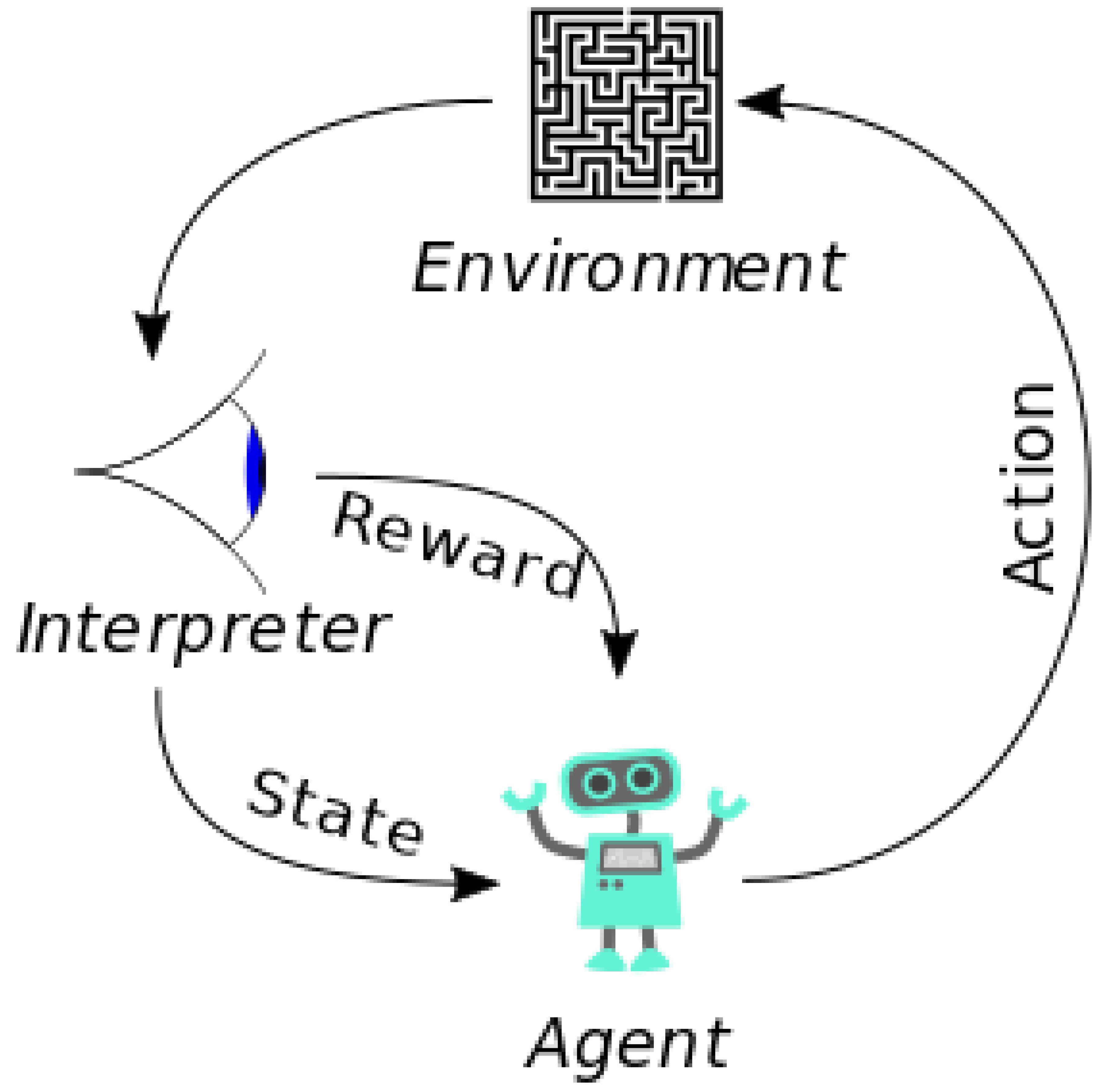
16.4.3. Mathematical Analysis of Reinforcement Learning
Reinforcement Learning (RL) is a framework for optimal decision-making in sequential environments where an agent interacts with a stochastic system to maximize a cumulative reward signal. Mathematically, RL is modeled as a Markov Decision Process (MDP), which is defined by the tuple , where S is the state space, A is the action space, is the transition probability of reaching state from state s after taking action a, is the reward function that defines the immediate reward received after executing action a in state s, and is the discount factor that determines the weight of future rewards.
The objective is to find an optimal policy that maximizes the expected cumulative reward over time, expressed as the return , defined by
The value function of a policy , denoted as , represents the expected return starting from state s while following policy ,
Similarly, the action-value function gives the expected return for taking action a in state s and subsequently following policy ,
The Bellman equation characterizes the value function recursively,
Similarly, the Bellman equation for the action-value function is given by
An optimal policy satisfies
and the optimal state-value function satisfies the Bellman optimality equation,
Similarly, the optimal action-value function satisfies
The policy iteration algorithm alternates between policy evaluation, which computes , and policy improvement, which updates the policy as
In contrast, value iteration directly updates using the Bellman optimality equation iteratively,
Temporal Difference (TD) learning updates value estimates based on observed transitions, using
The Q-learning algorithm updates the action-value function using the rule
where is the learning rate. In deep reinforcement learning, function approximators such as neural networks parameterized by approximate Q, where updates follow
The policy gradient method optimizes a stochastic policy by following the gradient of the expected return, given by
16.4.4. Python Code to Generate Figure 185
The Python code below produces the Figure 185 illustrating the Q-Learning policy.
Figure 185.
Q-Learning policy in a 4x4 grid world. Each cell shows the optimal action learned by the agent (↑, →, ↓, ←) to reach the goal. The agent learns the optimal path using reinforcement learning
Figure 185.
Q-Learning policy in a 4x4 grid world. Each cell shows the optimal action learned by the agent (↑, →, ↓, ←) to reach the goal. The agent learns the optimal path using reinforcement learning
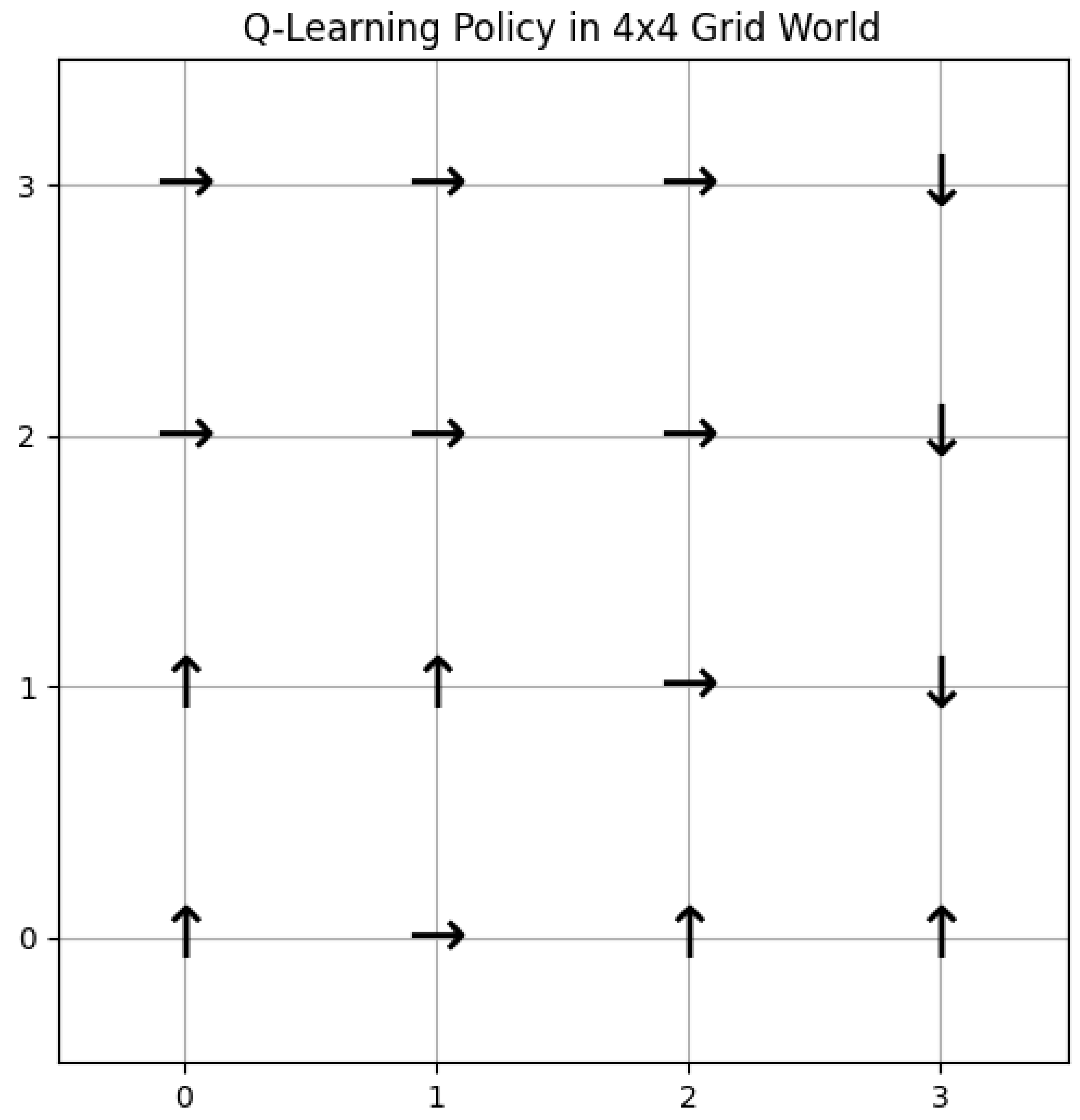
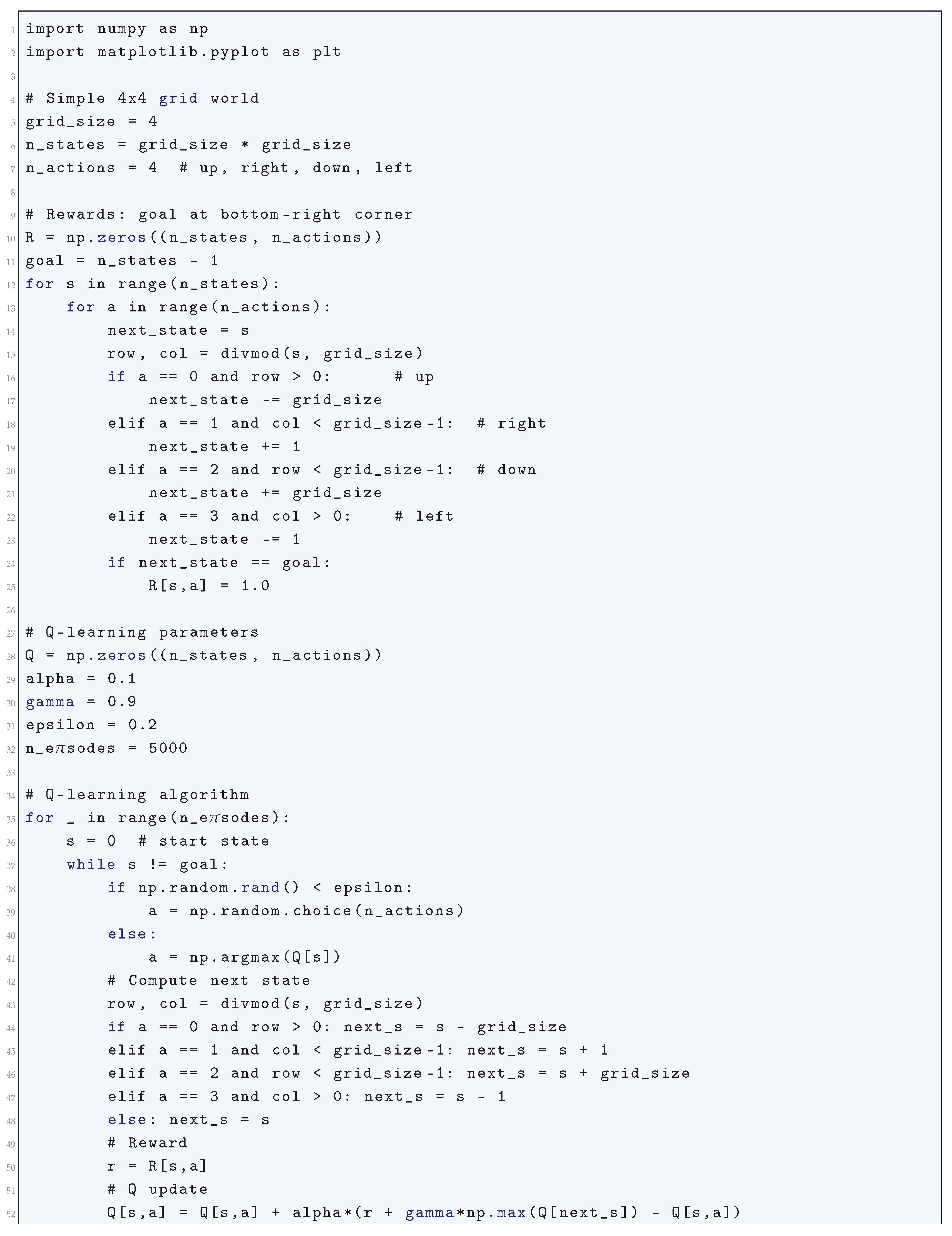
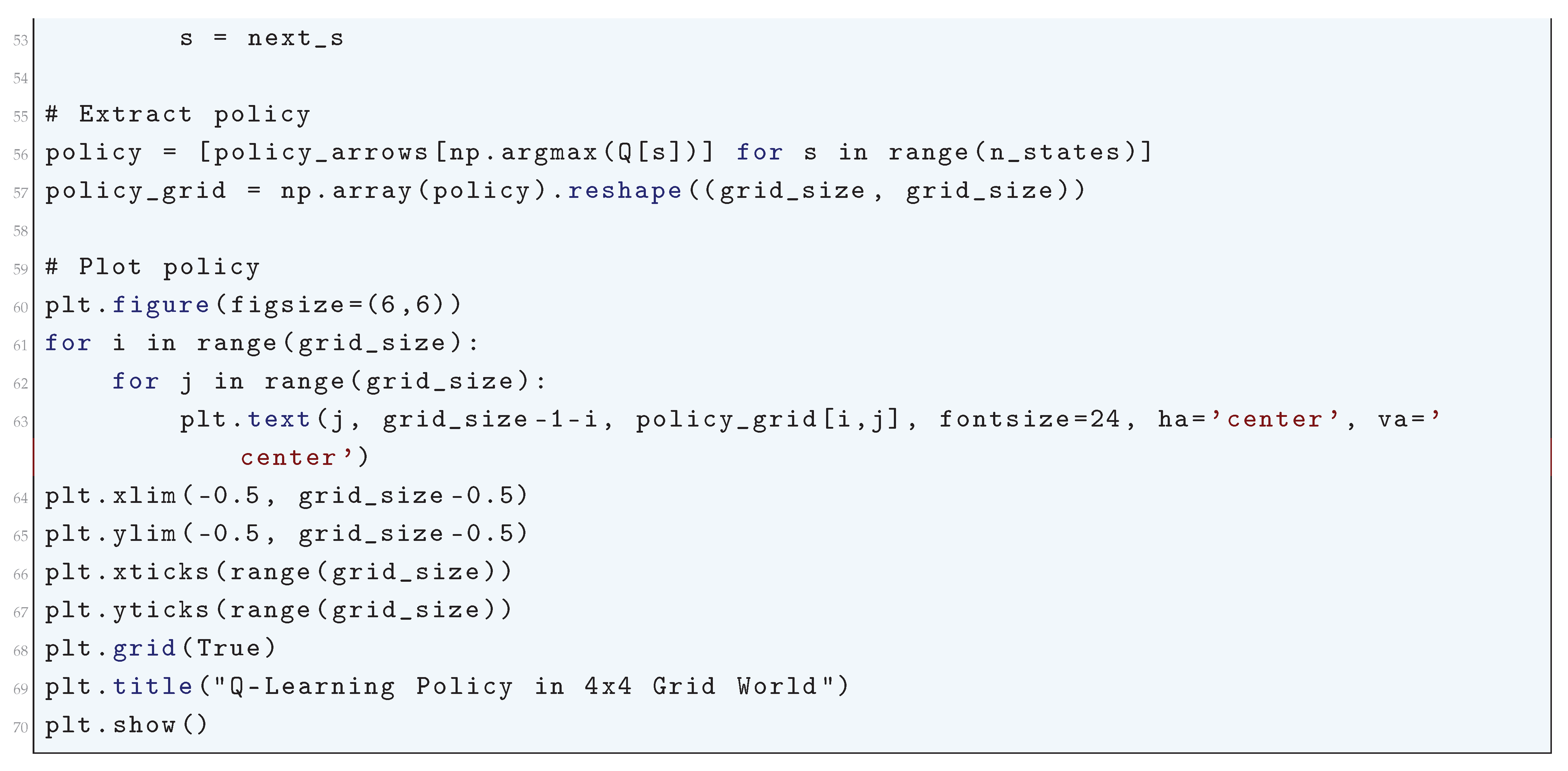
16.4.5. Policy Gradient Method
16.4.5.1 Literature Review of Policy Gradient Method
Policy gradient methods form a crucial class of reinforcement learning algorithms that directly optimize policies using gradient ascent techniques. The foundational work by Sutton et al. (1999) [906] introduced policy gradient methods in the context of function approximation, rigorously deriving an unbiased estimate of the gradient of the expected return. This work established the basis for parameterizing policies explicitly and developing gradient-based optimization techniques that ensure convergence under certain assumptions. Kakade (2001) [908] extended this framework by introducing the Natural Policy Gradient (NPG) method, which leverages the Fisher information matrix to normalize policy updates, thereby making learning more efficient and stable. The key contribution of NPG lies in its ability to make gradient updates invariant to policy parameterization, which enhances convergence properties and mitigates issues related to vanishing or exploding gradients.
Building upon these theoretical foundations, Schulman et al. (2015) [909] proposed Trust Region Policy Optimization (TRPO), which ensures monotonic improvement in policy performance by constraining the step size via the Kullback-Leibler (KL) divergence between successive policies. This theoretically motivated approach prevents drastic policy updates that could lead to performance degradation. TRPO was further refined by Schulman et al. (2017) [894] through Proximal Policy Optimization (PPO), which simplifies the optimization process by employing a clipped surrogate objective function. PPO strikes a balance between sample efficiency and computational feasibility, making it one of the most widely adopted algorithms in deep reinforcement learning. In parallel, Agarwal et al. (2021) [910] rigorously analyzed the optimality and sample complexity of policy gradient methods, particularly investigating how function approximation errors and distribution shifts affect their theoretical performance guarantees. Their work provided valuable insights into the conditions under which policy gradient methods converge to optimal or near-optimal policies.
Recent theoretical advancements, such as the work by Liu et al. (2024) [911], have further deepened our understanding of policy optimization by analyzing projected policy gradients and natural policy gradients in the context of discounted Markov Decision Processes (MDPs). By deriving novel convergence bounds, they provided an elementary yet rigorous framework that elucidates the dynamics of policy updates in large-scale reinforcement learning tasks. Meanwhile, Lorberbom et al. (2020) [912] proposed Direct Policy Gradients (DirPG), an alternative approach specifically designed for discrete action spaces. Their method optimizes policies by directly maximizing expected return-to-go trajectories, offering a novel perspective that integrates domain knowledge into policy optimization. Complementary to these efforts, McCracken et al. (2020) [913] studied policy gradient methods in exactly solvable Partially Observable Markov Decision Processes (POMDPs), deriving analytical results that characterize their probabilistic convergence behavior. Their findings are significant as they provide a rigorous theoretical foundation for understanding policy gradients in partially observable settings.
Lastly, practical considerations and comparative studies have played a crucial role in refining policy gradient methodologies. A definitive guide by Lehmann (2024) [914] systematically explores on-policy policy gradient methods in deep reinforcement learning, presenting a rigorous discussion of entropy regularization, KL divergence constraints, and their impact on stability. Furthermore, comparative analyses of policy-gradient algorithms done by Sutton et. al. (2000) [916] provide both theoretical and empirical evaluations of their efficiency and convergence properties, guiding practitioners in selecting the most suitable methods for various reinforcement learning applications. Collectively, these contributions have significantly advanced the theoretical underpinnings and practical implementations of policy gradient methods, shaping their role as a fundamental tool in modern reinforcement learning.
Table 45.
Summary of Key Contributions in Policy Gradient Methods
| Reference | Contribution |
| Sutton et al. (1999) | Introduced policy gradient methods with function approximation, deriving an unbiased gradient estimator for direct policy optimization. Established the foundation for parameterized policies independent of value functions. |
| Kakade (2001) | Developed Natural Policy Gradient (NPG), which utilizes the Fisher information matrix to normalize gradient updates, making learning invariant to policy parameterization. Improved stability and efficiency in policy optimization. |
| Schulman et al. (2015) | Proposed Trust Region Policy Optimization (TRPO), a theoretically motivated approach that enforces a KL divergence constraint on policy updates, ensuring monotonic performance improvement and preventing catastrophic performance drops. |
| Schulman et al. (2017) | Introduced Proximal Policy Optimization (PPO), which simplifies TRPO by using a clipped surrogate objective, striking a balance between computational efficiency and stability, making it widely adopted in deep reinforcement learning. |
| Agarwal et al. (2021) | Provided theoretical analysis on policy gradient optimality, sample complexity, and performance under distribution shift, giving insights into when policy gradient methods effectively converge to near-optimal solutions. |
| Liu et al. (2024) | Conducted a rigorous theoretical study on projected and natural policy gradients in discounted Markov Decision Processes (MDPs), deriving convergence rates and properties of different policy optimization methods. |
| Lorberbom et al. (2020) | Developed Direct Policy Gradients (DirPG), an approach optimized for discrete action spaces that maximizes return-to-go trajectories, allowing integration of domain knowledge into policy learning. |
| McCracken et al. (2020) | Analyzed policy gradient methods in exactly solvable Partially Observable Markov Decision Processes (POMDPs), deriving analytical results on value distributions and probabilistic convergence behavior. |
| Lehmann (2024) | Provided a definitive theoretical guide to policy gradients in deep reinforcement learning, covering entropy regularization, KL divergence constraints, and their impact on sample efficiency and stability. |
| Sutton et. al. (2000) | Conducted a comparative study on policy-gradient algorithms, evaluating their theoretical convergence properties and empirical efficiency, guiding practitioners in selecting appropriate methods. |
16.4.5.2 Recent Literature Review of Policy Gradient Method
Policy Gradient Methods in Reinforcement Learning (RL) have been widely adopted across various domains, leading to significant advancements in optimization, decision-making, and automation. One of the most notable implementations is in vehicular networks, where Mustafa et al. (2025) [917] leverage Proximal Policy Optimization (PPO) to manage computation offloading in vehicular communication systems. Their policy gradient-based framework optimally distributes computational resources across edge devices, reducing latency and improving system efficiency. Similarly, Yang et al. (2025) [918] employ a Deep Deterministic Policy Gradient (DDPG) in a hierarchical reinforcement learning (HRL) setup to dynamically optimize vehicular edge computing resources, outperforming traditional heuristics in real-time environments. These approaches collectively demonstrate the power of policy gradient methods in optimizing network performance under dynamic conditions. Additionally, Jamshidiha et al. (2025) [919] integrate Deep Deterministic Policy Gradient (DDPG) with Graph Neural Networks (GNNs) to improve mobile user association in cellular networks, dynamically optimizing traffic distribution and resource allocation. These approaches collectively demonstrate the power of policy gradient methods in optimizing network performance under dynamic conditions.
In the realm of robotic and autonomous control, policy gradient methods have enabled significant progress in task-specific learning. Raei et al. (2025) [920] introduce a DDPG-based reinforcement learning framework for robotic nonprehensile manipulation, particularly focusing on object sliding. Their study presents an efficient policy optimization technique that enhances robotic dexterity in handling objects without grasping them. Extending this concept to UAV (Unmanned Aerial Vehicle) applications, Ting-Ting et al. (2025) [921] propose a Multi-Agent Deep Deterministic Policy Gradient (MADDPG) approach, which allows multiple UAVs to make collaborative, autonomous decisions while operating under strict communication constraints. Similarly, Zhang et al. (2025) [922] integrate Deep Deterministic Policy Gradient (DDPG) with neuromorphic computing to develop a novel Hybrid Deep Deterministic Policy Gradient (Neuro-HDDPG) algorithm. This approach enhances obstacle avoidance for spherical underwater robots by mimicking the decision-making process of biological neural networks, significantly improving their autonomy in complex underwater environments.
Policy gradient methods have also found profound applications in reinforcement learning for natural language processing (NLP) and constrained decision-making problems. Nguyen et al. (2025) [923] explore REINFORCE and RELAX policy gradient algorithms to fine-tune text-to-SQL models, effectively improving structured query generation accuracy by optimizing reward-based learning. Additionally, Chathuranga Brahmanage et al. (2025) [924] extend policy gradient techniques to action-constrained reinforcement learning by leveraging constraint violation signals, allowing agents to optimize their decision-making while adhering to predefined operational constraints. These studies highlight how policy gradient approaches can be adapted to complex, structured learning tasks that require precision and rule adherence.
Another major advancement in policy gradient methods is in federated learning and network optimization. Huang et al. (2025) [925] introduce the Knowledge Collaboration Actor-Critic Policy Gradient (KCACPG) algorithm, which facilitates knowledge transfer in cooperative traffic scheduling for intelligent transportation networks, ensuring seamless traffic management with minimal delays. Finally, Li et al. (2025) [926] propose FedDDPG, a federated learning variant of Deep Deterministic Policy Gradient, tailored for vehicle trajectory prediction in decentralized learning environments. This framework enables autonomous vehicles to learn optimal path planning strategies without centralizing sensitive data, ensuring enhanced privacy and efficiency in large-scale intelligent transportation systems. Together, these contributions showcase the robustness of policy gradient methods across diverse applications, reinforcing their critical role in advancing deep reinforcement learning frameworks for real-world challenges.
| Authors (Year) | Contribution |
| Mustafa et al. (2025) | Utilizes Proximal Policy Optimization (PPO) to optimize offloading decisions in vehicular communication networks, reducing latency and enhancing efficiency. |
| Huang et al. (2025) | Introduces the Knowledge Collaboration Actor-Critic Policy Gradient (KCACPG) method to optimize reinforcement learning in traffic management using knowledge transfer. |
| Yang et al. (2025) | Employs Deep Deterministic Policy Gradient (DDPG) within a hierarchical reinforcement learning framework to optimize vehicular resource allocation. |
| Jamshidiha et al. (2025) | Combines Graph Neural Networks (GNN) with DDPG to improve mobile user association in cellular networks through dynamic traffic-aware optimization. |
| Raei et al. (2025) | Develops a DDPG-based framework for robotic nonprehensile manipulation, enabling efficient object sliding with adaptive policy gradient optimization. |
| Ting-Ting et al. (2025) | Proposes a Multi-Agent Deep Deterministic Policy Gradient (MADDPG) algorithm to optimize UAV coordination under limited communication conditions. |
| Zhang et al. (2025) | Integrates neuromorphic computing with reinforcement learning to develop a Hybrid Deep Deterministic Policy Gradient (Neuro-HDDPG) for underwater robot navigation. |
| Nguyen et al. (2025) | Implements REINFORCE and RELAX policy gradient algorithms to improve text-to-SQL model fine-tuning with reward optimization. |
| Chathuranga Brahmanage et al. (2025) | Introduces a constraint-aware policy gradient algorithm that learns from violation signals, optimizing decision-making within strict operational constraints. |
| Li et al. (2025) | Proposes FedDDPG, a federated learning extension of Deep Deterministic Policy Gradient (DDPG) to optimize vehicle trajectory prediction while preserving data privacy. |
16.4.5.3 Mathematical Analysis of Policy Gradient Method
The policy gradient method is a fundamental approach in reinforcement learning that directly optimizes the policy , parameterized by , through gradient ascent on an objective function that represents expected cumulative rewards. The policy defines a probability distribution over actions given a state, and the goal is to adjust such that the expected return is maximized. The objective function, representing the expected return, is given by
where represents a trajectory sampled from the environment following policy , and is the probability distribution over trajectories under policy , given by the product of the initial state distribution , the policy probability, and the state transition dynamics:
The reward function is typically defined as the sum of discounted rewards:
where is the reward received at time step t and is the discount factor.
The gradient of with respect to is computed using the likelihood ratio trick:
Expanding the logarithm,
we obtain
This expectation is estimated using Monte Carlo sampling over trajectories:
where are sampled trajectories. Instead of using raw returns , it is common to replace them with an advantage function to reduce variance:
where is the action-value function,
and is the state-value function,
Replacing with , the gradient estimate becomes
The parameters are updated using gradient ascent:
where is the learning rate. A commonly used baseline function , often taken as , is subtracted to further reduce variance without introducing bias:
This formulation forms the basis of policy gradient methods, including REINFORCE, actor-critic algorithms, and proximal policy optimization (PPO), which introduce additional constraints and refinements to improve stability and efficiency.
16.4.5.4 Python Code to Generate Figure 186
The Python code below produces the Figure 186 illustrating the Policy Gradient Method.
Figure 186.
Policy Gradient Method: The policy network (green) outputs a distribution over actions given the state. The environment (gray) produces trajectories and rewards, which are stored (orange). The policy gradient update (red) adjusts the policy parameters using the gradient
Figure 186.
Policy Gradient Method: The policy network (green) outputs a distribution over actions given the state. The environment (gray) produces trajectories and rewards, which are stored (orange). The policy gradient update (red) adjusts the policy parameters using the gradient
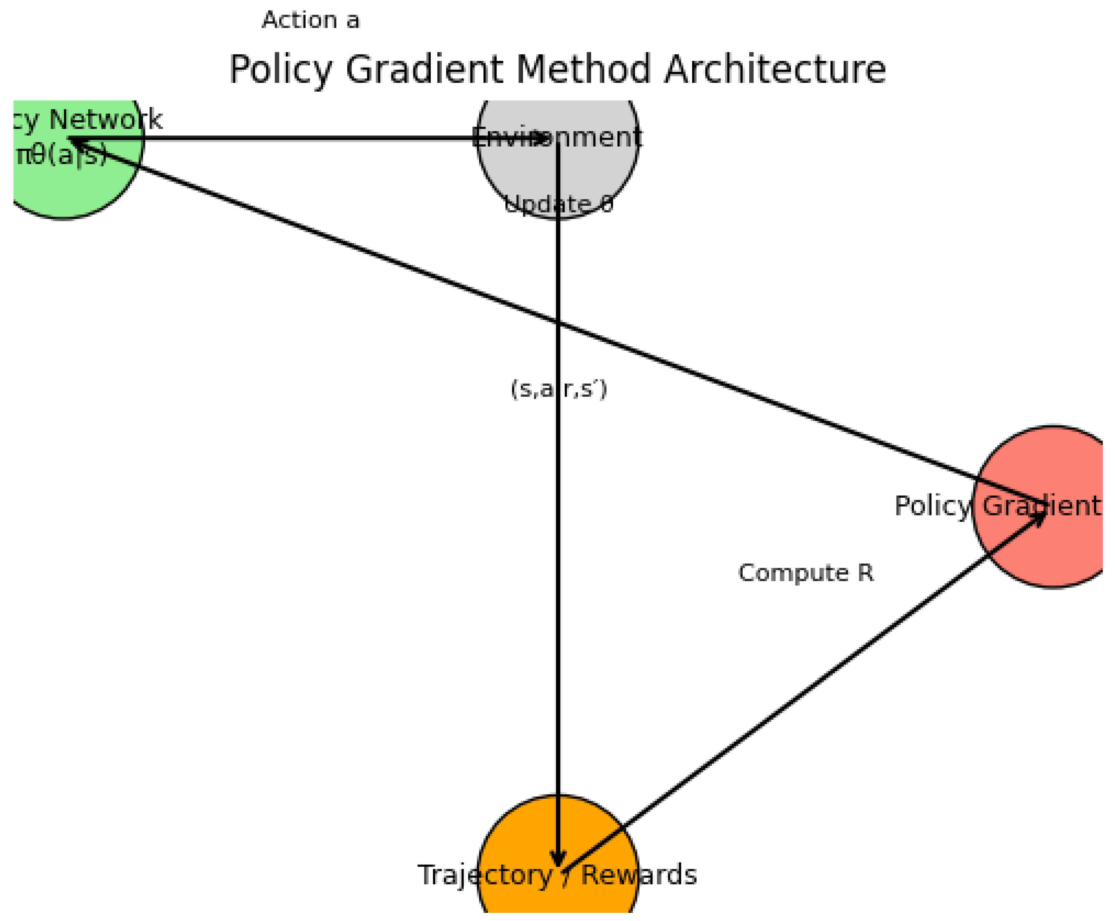
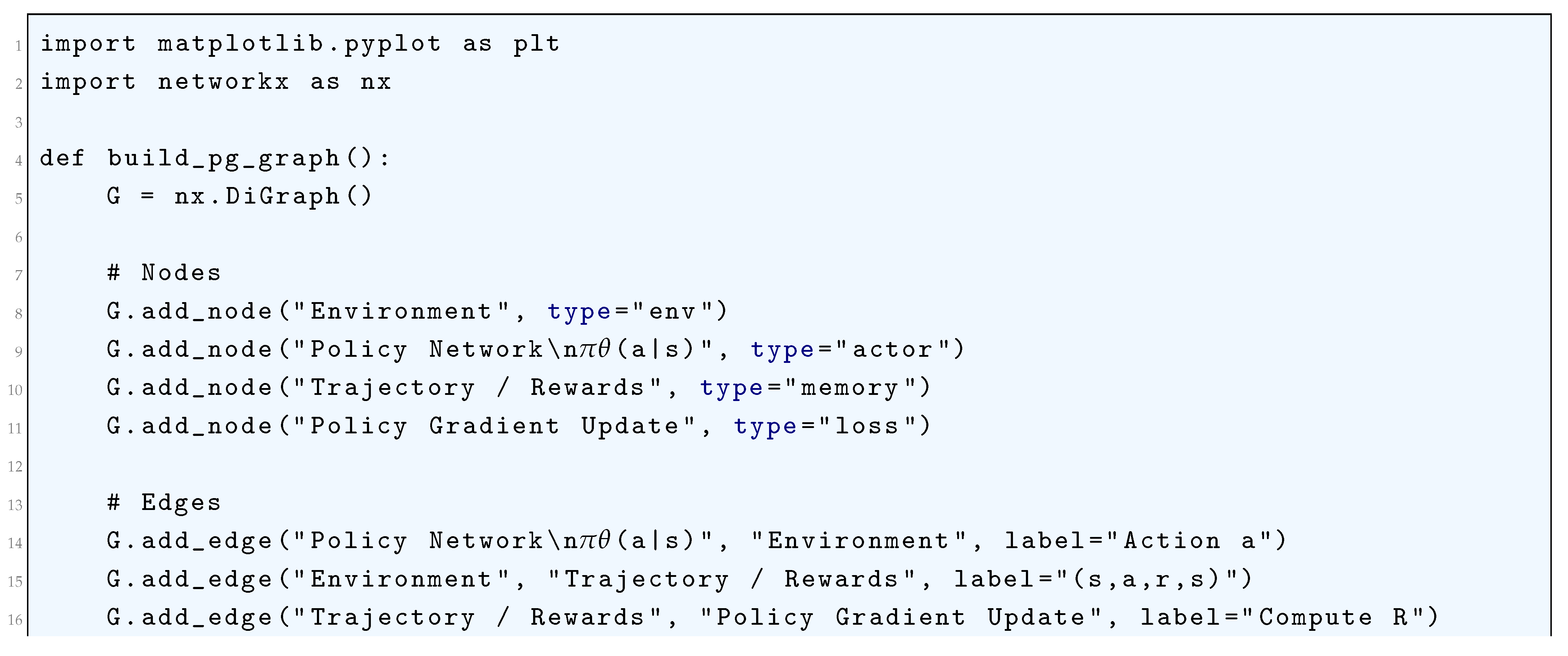
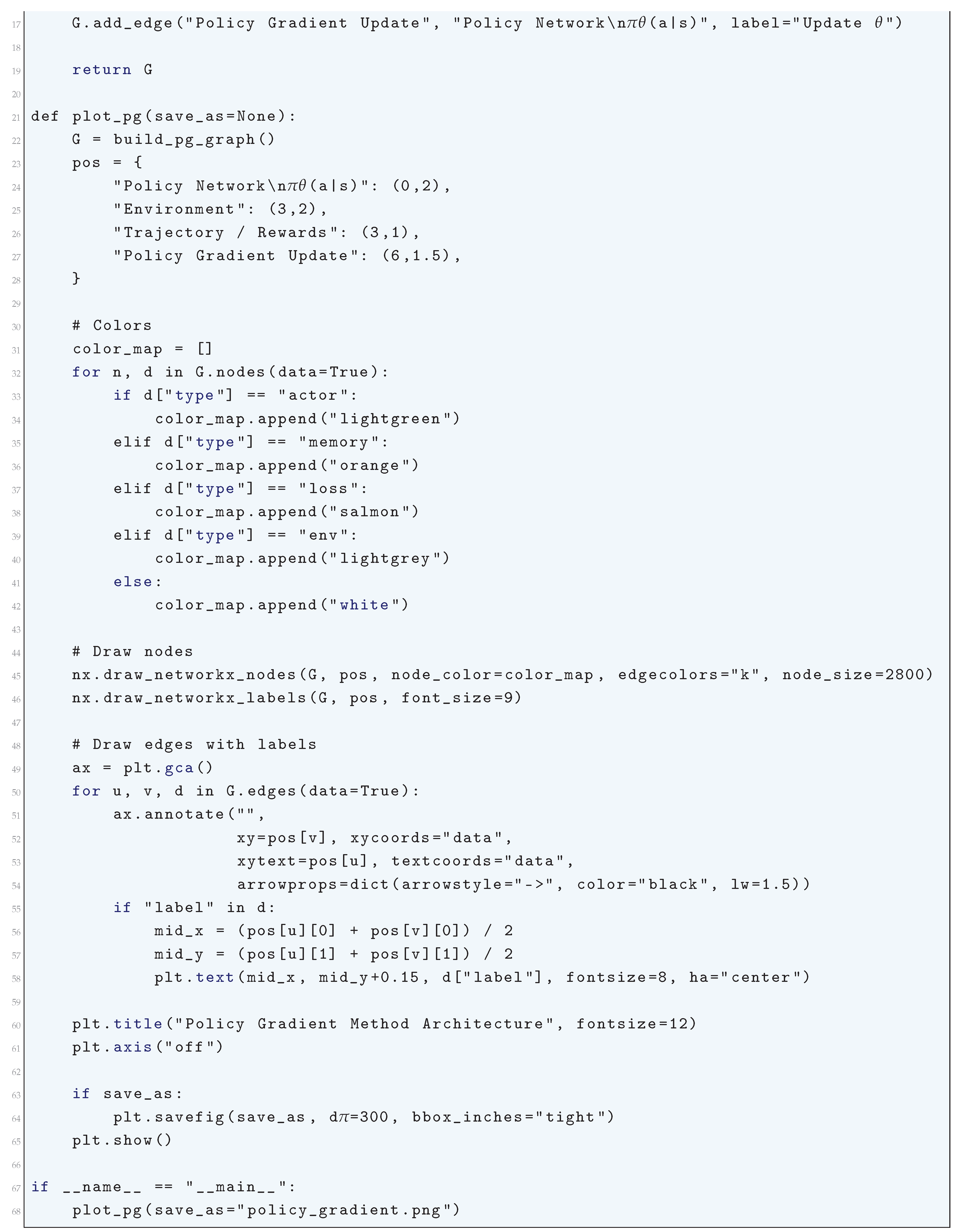
16.4.6. Deep Reinforcement Learning
16.4.6.1 Literature Review of Deep Reinforcement Learning
Deep Reinforcement Learning (DRL) has undergone significant advancements over the past decade, driven by key innovations in value-based methods, policy optimization, and distributional approaches. The introduction of Deep Q-Networks (DQN) by Mnih et al. (2015) [292] marked a turning point, demonstrating that deep neural networks could successfully approximate Q-values for high-dimensional state spaces. The stability of DQN was ensured through experience replay, which mitigated correlation among consecutive updates, and target networks, which provided a stable reference for temporal difference updates. However, DQN was restricted to discrete action spaces, prompting Lillicrap et al. (2016) [895] to introduce the Deep Deterministic Policy Gradient (DDPG), an actor-critic method designed for continuous control problems. DDPG extended Q-learning to continuous actions by utilizing an off-policy approach with target smoothing, improving convergence in high-dimensional environments. Meanwhile, Schulman et al. (2015) [909], Schulman et al. (2017) [894] introduced Trust Region Policy Optimization (TRPO) and Proximal Policy Optimization (PPO), which formulated policy optimization with explicit constraints on divergence from previous policies. PPO’s clipped objective made it computationally efficient and less sensitive to hyperparameters, establishing it as a standard for training deep RL agents.
Building upon these foundations, Haarnoja et al. (2018) [291] proposed Soft Actor-Critic (SAC), which incorporated entropy maximization to encourage exploration and robustness in policy learning. Unlike traditional policy gradient methods, SAC optimized a trade-off between reward accumulation and policy stochasticity, leading to superior performance in complex robotic tasks. Simultaneously, Hessel et al. (2018) [927] developed Rainbow DQN, a unification of multiple enhancements to DQN, including Double DQN, Prioritized Experience Replay, Dueling Networks, Multi-step Learning, Noisy Networks, and Distributional RL. This integration provided a comprehensive framework for improving sample efficiency and generalization. Reinforcement learning also made breakthroughs in strategic decision-making, as demonstrated by Silver et al. (2016) [892] with AlphaGo, which leveraged Monte Carlo Tree Search (MCTS) with deep policy and value networks to achieve superhuman performance in the game of Go. AlphaGo’s success was a milestone in planning-based RL, where deep neural networks provided heuristic guidance for complex search-based decision-making.
Another significant area of advancement in DRL was its application to robotic control and perception-driven decision-making. Levine et al. (2016) [928] pioneered end-to-end deep visuomotor policies, allowing robots to learn manipulation skills directly from raw visual inputs. Their work integrated guided policy search with deep learning, enabling robots to generalize across unseen scenarios with improved sample efficiency. Parallel to these practical advancements, theoretical contributions were made by Bellemare et al. (2017) [929] in Distributional RL, which proposed predicting a distribution of future rewards rather than a single expected return. This perspective significantly improved stability and sample efficiency, leading to the development of quantile-based methods like QR-DQN and Implicit Quantile Networks (IQN). Additionally, the foundational work by Sutton (2018) [286] provided a rigorous mathematical exposition of value iteration, policy iteration, and temporal difference learning, forming the theoretical bedrock of modern RL research. Their book continues to be the definitive reference for both theoretical exploration and practical implementation of reinforcement learning algorithms.
Through these fundamental breakthroughs, DRL has evolved into a robust field that spans value-based methods, policy gradient approaches, entropy-regularized reinforcement learning, and distributional perspectives. The fusion of deep learning with reinforcement learning has enabled unprecedented progress in areas such as robotics, strategic decision-making, and autonomous systems. The field continues to expand, with ongoing research exploring meta-reinforcement learning, multi-agent RL, and offline reinforcement learning to push the boundaries of intelligent decision-making in complex and uncertain environments.
Table 46.
Summary of Contributions in Deep Reinforcement Learning
| Reference | Contribution |
| Mnih et al. (2015) | Introduced Deep Q-Learning for high-dimensional state spaces using deep neural networks. Proposed experience replay to break correlation among samples and target networks for stable Q-value updates. Enabled deep reinforcement learning for discrete action spaces. |
| Lillicrap et al. (2016) | Extended Q-learning to continuous action spaces using an actor-critic framework. Leveraged off-policy learning with target smoothing to improve convergence and stability in high-dimensional environments. |
| Schulman et al. (2015) | Developed a stable policy gradient method with constraints on policy divergence using a trust region approach. Ensured monotonic policy improvement and was particularly effective in robotic control tasks. |
| Schulman et al. (2017) | Simplified TRPO by introducing a clipped surrogate objective for stable and efficient policy updates. Achieved state-of-the-art performance while being computationally efficient and less sensitive to hyperparameters. |
| Haarnoja et al. (2018) | Introduced entropy-regularized reinforcement learning to encourage exploration. Optimized a stochastic policy while balancing reward accumulation and entropy maximization, improving sample efficiency and robustness. |
| Hessel et al. (2018) | Unified multiple improvements to DQN, including Double DQN, Prioritized Experience Replay, Dueling Networks, Multi-step Learning, Noisy Networks, and Distributional RL. Provided a comprehensive framework with enhanced sample efficiency and stability. |
| Silver et al. (2016) | Combined Monte Carlo Tree Search (MCTS) with deep policy and value networks to achieve superhuman performance in the game of Go. Demonstrated the power of planning-based reinforcement learning. |
| Levine et al. (2016) | Integrated deep learning with guided policy search for end-to-end robotic manipulation. Enabled robots to learn complex tasks directly from raw visual inputs. |
| Bellemare et al. (2017) | Proposed predicting the distribution of future rewards instead of the expected value. Led to improved stability and sample efficiency, forming the foundation for quantile-based RL methods such as QR-DQN and IQN. |
| Sutton and Barto (2018) | Provided a rigorous mathematical foundation for reinforcement learning. Covered fundamental topics such as value iteration, policy iteration, and temporal difference learning. Served as a definitive reference for both theoretical and practical RL research. |
16.4.6.2 Recent Literature Review of Deep Reinforcement Learning
Deep reinforcement learning (DRL) has emerged as a powerful tool for solving complex decision-making and control problems across various domains. One of its key applications is in task offloading and resource allocation in mobile edge computing (MEC) networks, particularly in UAV-assisted environments. The work by Xue et al. (2025) [930] proposes a novel DRL-based algorithm to optimize computation offloading and multi-cache placement, addressing efficiency bottlenecks in UAV-assisted MEC systems. This is complemented by Amodu et al. (2025) [931], who present a comprehensive review of DRL applications for UAV-based optimization in MEC and IoT applications. Their work outlines the core challenges of DRL, including sample inefficiency, high computational costs, and model generalizability, while also suggesting future directions such as transfer learning and meta-reinforcement learning to improve adaptability in real-world systems. Another critical area where DRL has proven useful is autonomous energy management, as demonstrated in the study by Sunder et al. (2025) [932], who introduce the SmartAPM framework. This system leverages DRL to optimize power consumption in wearable devices, allowing for extended battery life through adaptive power control strategies based on environmental and user activity data.
Beyond network optimization and energy management, DRL is also making significant strides in autonomous control systems and cyber defense. For instance, Sarigül and Bayezit (2025) [933] apply DRL to fixed-wing aircraft heading control, showing how deep policy optimization can enhance maneuverability and operational autonomy compared to classical control techniques. Similarly, Mustafa et al. (2025) [917] focus on vehicular networks, proposing a Proximal Policy Optimization (PPO)-based DRL framework for computation offloading. Their findings highlight improved latency reduction and energy efficiency, making real-time decision-making more feasible for intelligent transport systems. Meanwhile, Mukhamadiarov (2025) [934] explores the application of DRL in stochastic dynamical systems, demonstrating how reinforcement learning can be effectively integrated with traditional control theory to enhance stability in non-linear environments. In cybersecurity, Ali and Wallace (2025) [935] introduce a DRL-powered autonomous cyber defense system for Security Operations Centers (SOCs), where self-learning agents continuously refine threat detection and mitigation strategies in adversarial settings. This research underscores the increasing role of DRL in adaptive cyber resilience, as it allows security systems to proactively identify and neutralize cyber threats in real-time.
Another promising area of DRL research lies in cross-domain transfer learning and real-world deployment, particularly in fluid dynamics and energy optimization. The study by Yan et al. (2025) [936] applies a mutual information-based transfer learning approach in active flow control for three-dimensional bluff body flows, significantly reducing training costs by enabling efficient knowledge transfer between different aerodynamic configurations. In a different sector, Silvestri et al. (2025) [937] investigated the deployment of DRL in real-world building control systems, where they incorporate imitation learning to address the sample inefficiency problem that plagues traditional DRL methods. Their approach enhances energy efficiency in buildings while maintaining occupant comfort, demonstrating a viable path for scaling DRL beyond theoretical applications. Similarly, Alajaji et al. (2025) [938] provide a scoping review of DRL in medical imaging, particularly in infrared spectroscopy-based cancer diagnosis. Their findings reveal that DRL can significantly improve the sensitivity and specificity of early cancer detection by automatically identifying abnormal patterns in spectroscopy data.
Collectively, these studies showcase the remarkable versatility and potential of DRL in solving real-world challenges. Whether in network optimization, cyber defense, autonomous control, medical imaging, or fluid dynamics, DRL continues to redefine the boundaries of machine learning by offering adaptive, scalable, and self-improving solutions. However, challenges such as high sample complexity, lack of explainability, and computational overhead remain significant hurdles that researchers are actively working to overcome. Future research in DRL is likely to focus on hybrid learning approaches, transfer learning techniques, and improved generalization methods to ensure that DRL models can perform effectively across diverse, unpredictable environments. The continued evolution of DRL in these domains not only paves the way for more robust and intelligent autonomous systems but also holds promise for breakthroughs in fields ranging from aerospace engineering to healthcare and cybersecurity.
Table 47.
Summary of Recent Contributions in Deep Reinforcement Learning Research
| Authors (Year) | Contribution |
| K. Xue, L. Zhai, Y. Li, Z. Lu, W. Zhou (2025) | Proposes a DRL-based algorithm to optimize task offloading and caching in UAV-assisted MEC networks, addressing computational efficiency and resource allocation. |
| O.A. Amodu, R.A.R. Mahmood, H. Althumali (2025) | Provides a comprehensive review of DRL applications in UAV-based MEC and IoT systems, identifying challenges and proposing future research directions. |
| A. Silvestri, D. Coraci, S. Brandi, A. Capozzoli (2025) | Investigates imitation learning as an alternative to DRL for real-world building control systems to enhance energy efficiency while maintaining occupant comfort. |
| R. Sunder, U.K. Lilhore, A.K. Rai, E. Ghith, M. Tlija (2025) | Introduces SmartAPM, a DRL-based adaptive power management system that optimizes battery life based on environmental and user activity data. |
| L. Yan, Q. Wang, G. Hu, W. Chen, B.R. Noack (2025) | Develops a mutual information-based transfer learning approach for DRL in active flow control, reducing training costs and improving aerodynamic simulations. |
| E. Mustafa, J. Shuja, F. Rehman, A. Namoun (2025) | Proposes a PPO-based DRL framework for vehicular computation offloading, significantly improving latency and energy efficiency in intelligent transport systems. |
| S.A. Alajaji, R. Sabzian, Y. Wang, A.S. Sultan, R. Wang (2025) | Reviews the use of DRL in medical imaging, highlighting its potential in infrared spectroscopy-based cancer diagnosis for improved accuracy and early detection. |
| N. Ali, G. Wallace (2025) | Explores DRL applications in cybersecurity, particularly in autonomous cyber defense for SOCs, enhancing threat detection and response capabilities. |
| F.A. Sarigül, I. Bayezit (2025) | Applies DRL to fixed-wing aircraft heading control, improving maneuverability and autonomy over traditional control techniques. |
| R. Mukhamadiarov (2025) | Investigates the application of DRL for controlling stochastic dynamical systems by integrating reinforcement learning with control theory to optimize stability. |
16.4.6.3 Mathematical Analysis of Deep Reinforcement Learning
Deep Reinforcement Learning (DRL) is a mathematical framework that extends classical Reinforcement Learning (RL) by leveraging deep neural networks to approximate complex functions, enabling the efficient handling of high-dimensional state and action spaces. Mathematically, DRL is rooted in the Markov Decision Process (MDP), which is formally defined as the tuple
where is the state space, is the action space, represents the transition probability function defining the probability of transitioning to state given the current state s and action a, is the reward function specifying the immediate reward received after taking action a in state s, and is the discount factor that determines the present value of future rewards. The objective of DRL is to find an optimal policy that maximizes the expected cumulative reward, given by the return function:
The optimal policy is derived by maximizing the state-value function or the action-value function , which are respectively defined as:
In Deep Q-Networks (DQN), a deep neural network parameterized by is used to approximate the optimal Q-function:
The network parameters are updated using the loss function derived from the Bellman equation:
where y is the target value computed using the Bellman optimality equation:
where represents the parameters of a target network that is updated periodically to stabilize training.
Policy-based methods directly optimize the policy without relying on a Q-function. The objective function for policy gradient methods is given by:
The gradient of with respect to the policy parameters is computed using the policy gradient theorem:
The REINFORCE algorithm estimates this gradient using Monte Carlo sampling:
Actor-Critic methods combine value-based and policy-based approaches by introducing an actor network and a critic network , where w represents the critic parameters. The critic updates its parameters using the Temporal Difference (TD) error:
The policy gradient is then computed using an advantage function , where:
In Advantage Actor-Critic (A2C), the policy gradient update is:
Deep Deterministic Policy Gradient (DDPG) extends policy gradients to continuous action spaces by parameterizing the policy as a deterministic function:
The policy update follows the deterministic policy gradient theorem:
Proximal Policy Optimization (PPO) improves stability by enforcing a trust region constraint on policy updates. The surrogate objective function is:
where is the probability ratio between the new and old policies. Soft Actor-Critic (SAC) introduces an entropy regularization term to encourage exploration:
where represents the entropy of the policy, and is a temperature parameter.
16.4.6.3.1 Python Code to Generate Figure 187
The Python code below produces the Figure 187 illustrating the Deep Reinforcement Learning.
Figure 187.
General pipeline of Deep Reinforcement Learning (DRL): The agent, represented by a deep neural network (blue), interacts with the environment (gray) by producing actions. The environment generates experiences, which are stored in the replay buffer (orange). Mini-batches from the buffer are used to compute predictions and targets for the loss function (red). The optimizer (violet) updates network weights through gradient descent
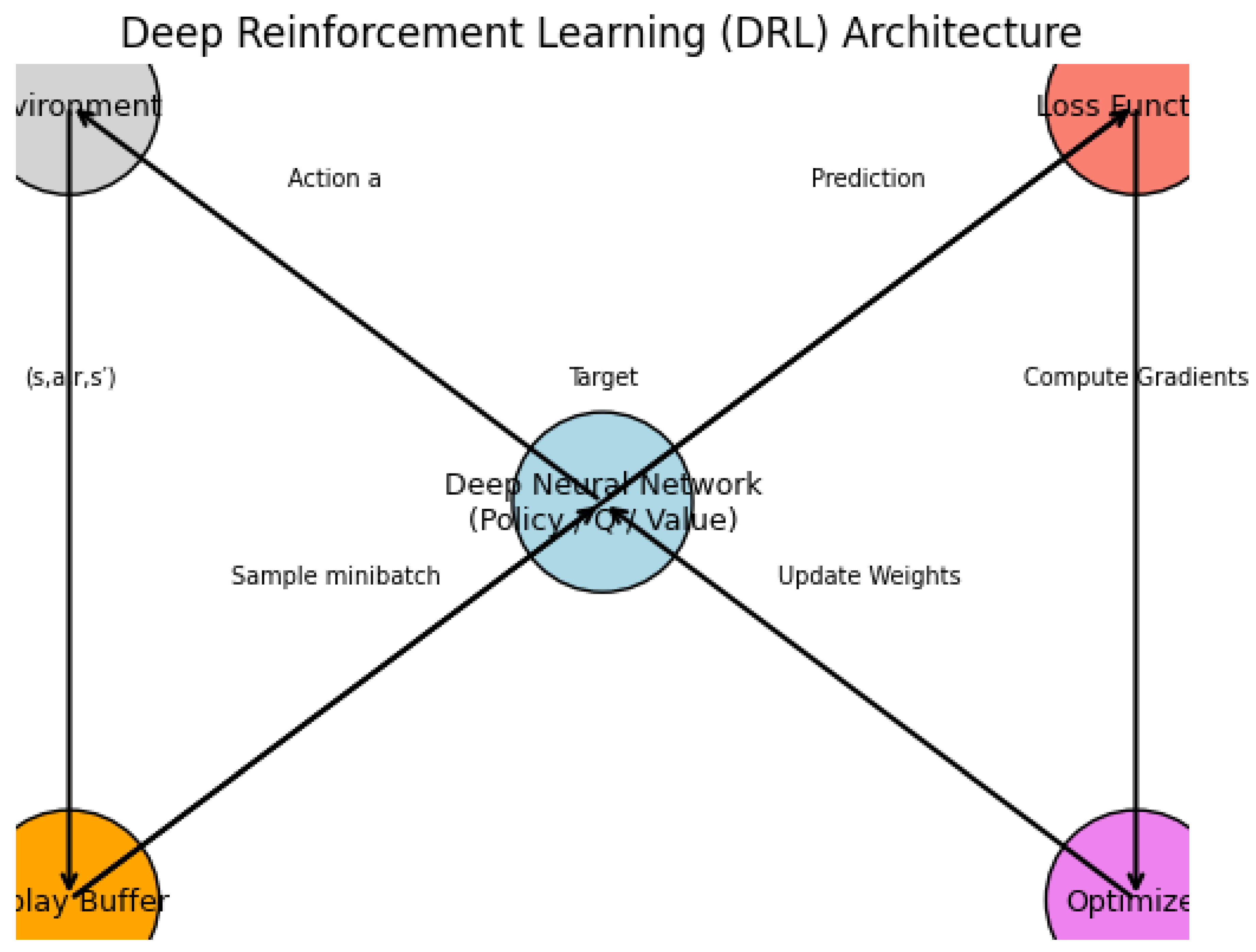
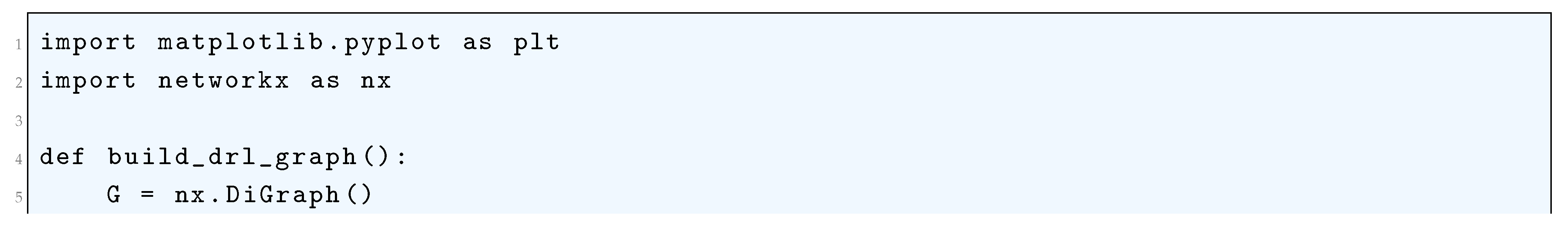
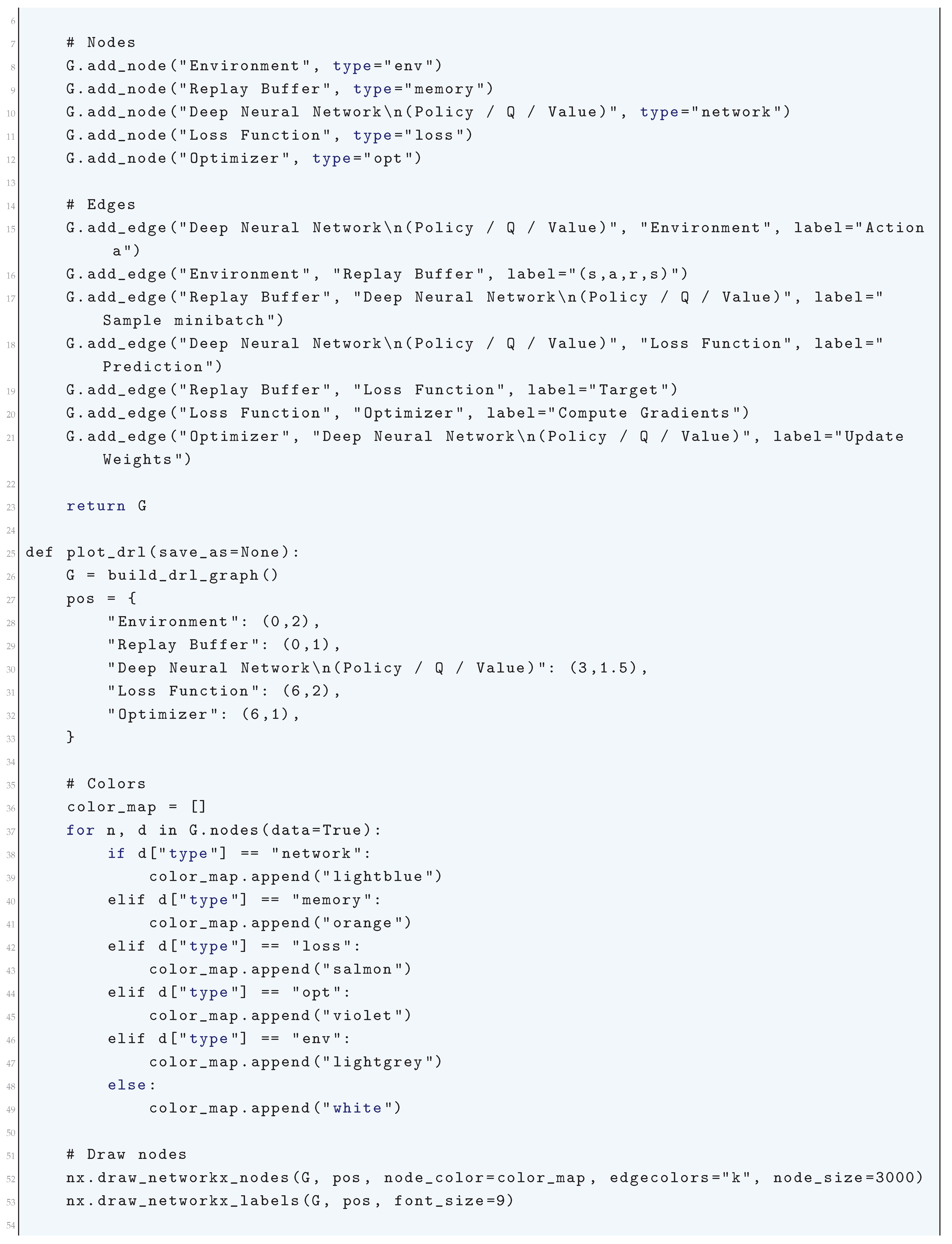
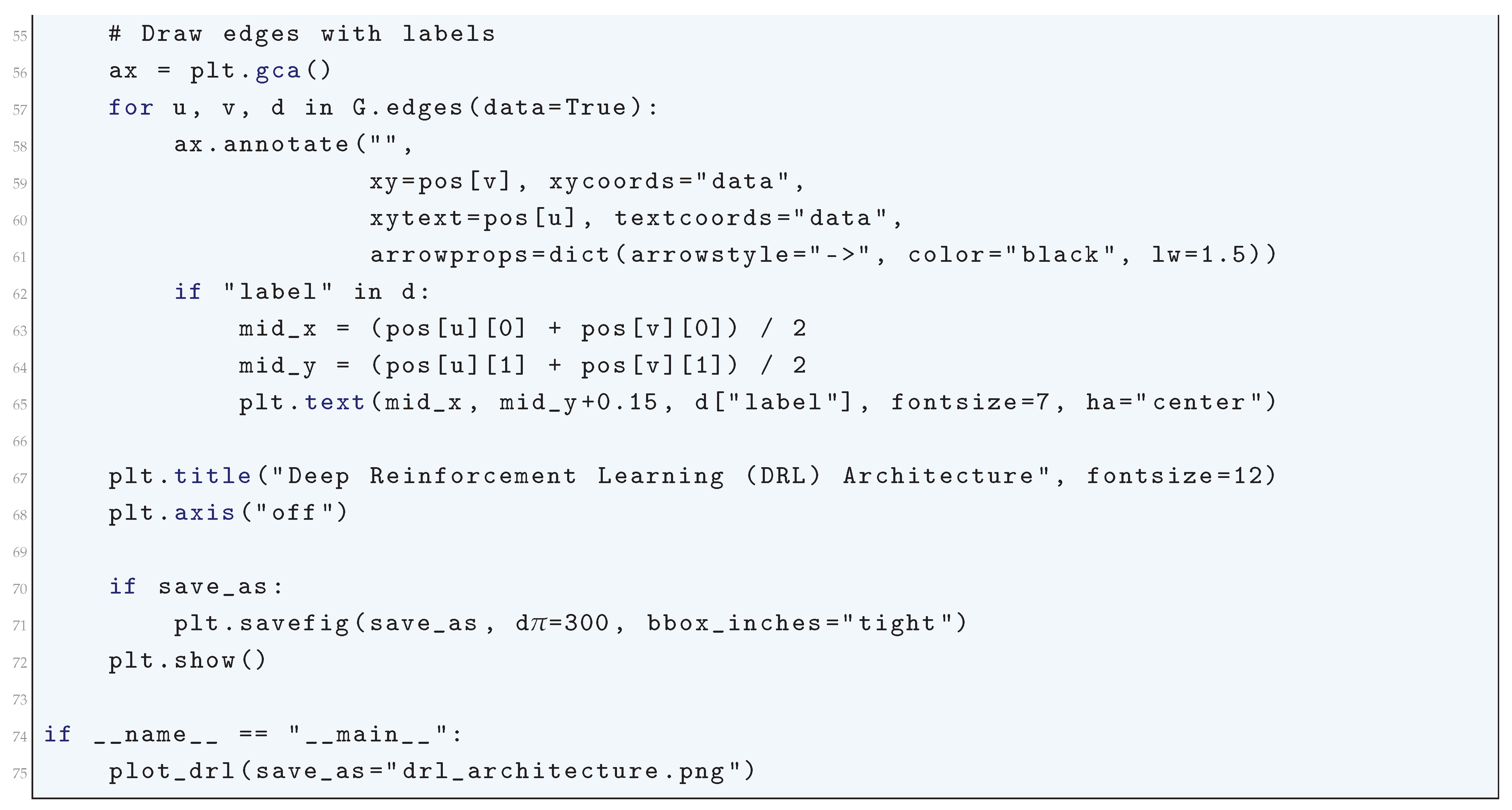
16.4.6.4 Advantage Actor-Critic (A2C)
16.4.6.4.1 Literature Review of Advantage Actor-Critic (A2C)
The Advantage Actor-Critic (A2C) algorithm has been extensively studied and applied in various domains, contributing to both theoretical advancements and practical implementations. Mnih et al. (2016) [949] laid the foundational work for A2C through their development of the Asynchronous Advantage Actor-Critic (A3C) method, which utilized multi-threaded parallelization to stabilize policy gradient methods. A2C emerged as a synchronous variant that improved sample efficiency while retaining the stability benefits of A3C. Wang et al. (2022) [950] further refined A2C by introducing Recursive Least Squares (RLS) methods to improve sample efficiency and convergence stability. Their research focused on optimizing the learning process using adaptive step sizes, effectively reducing training time and enhancing the robustness of deep reinforcement learning models.
The adaptability of A2C has enabled its application across diverse fields, including financial market trading and multi-agent reinforcement learning. Rubell Marion Lincy et al. (2023) [951] explored the integration of A2C with technical analysis indicators to improve decision-making in stock trading. Their approach demonstrated that A2C could effectively learn optimal buy and sell strategies while adapting to market fluctuations. Meanwhile, Paczolay et al. (2020) [952] extended A2C to multi-agent environments, addressing key challenges in coordination and competition. They developed an improved training mechanism to stabilize interactions between multiple learning agents, significantly enhancing performance in decentralized decision-making settings. Zhang et al. (2024) [953] leveraged A2C for industrial applications, specifically in disassembly line balancing, where they optimized cycle time minimization. By formulating the optimization problem as a reinforcement learning task, they showcased the potential of A2C to streamline complex industrial processes.
Beyond conventional applications, researchers have also explored novel enhancements to A2C, such as quantum computing and adversarial training. Kölle et al. (2024) [955] introduced Quantum Advantage Actor-Critic (QA2C) and Hybrid Advantage Actor-Critic (HA2C), benchmarking them against classical A2C implementations. Their findings indicated that quantum models could improve computational efficiency, making reinforcement learning more scalable for high-dimensional problems. Benhamou (2019) [956] focused on addressing one of the fundamental challenges in policy gradient methods—variance reduction. By formulating a rigorous mathematical framework, they optimized control variate estimators, effectively minimizing gradient variance and improving learning stability. Similarly, Peng et al. (2018) [957] introduced Adversarial A2C, where a discriminator was incorporated to enhance exploration strategies in dialogue policy learning. Their approach demonstrated significant improvements in reinforcement learning-based conversational agents, particularly in human-like task completion.
Finally, A2C has proven to be a powerful tool in robotics and adaptive control systems. Van Veldhuizen (2022) [958] explored its application in tuning Proportional-Integral-Derivative (PID) controllers for robotic systems. Their research demonstrated that A2C could autonomously optimize PID parameters, significantly improving the precision of control tasks such as apple harvesting. The ability of A2C to generalize across different control environments underscores its flexibility as a reinforcement learning framework. Collectively, these contributions illustrate the extensive theoretical advancements and practical innovations enabled by A2C, solidifying its position as a cornerstone in deep reinforcement learning.
Table 48.
Summary of Contributions in A2C Research
| Reference | Contribution |
| Mnih et al. (2016) | Introduced the Asynchronous Advantage Actor-Critic (A3C) algorithm, which inspired the synchronous A2C algorithm by stabilizing policy gradient methods through multi-threaded training. |
| Wang et al. (2022) | Developed RLS-based A2C variants that improve sample efficiency and learning stability in deep reinforcement learning environments. |
| Rubell Marion Lincy et al. (2023) | Applied A2C for stock trading using technical indicators, showing improved decision-making for buy and sell strategies. |
| Paczolay et al. (2020) | Adapted A2C for multi-agent scenarios, addressing coordination and competition among agents with improved training mechanisms. |
| Zhang et al. (2024) | Applied A2C for industrial optimization problems, demonstrating enhanced cycle time minimization in disassembly line balancing. |
| Kölle et al. (2024) | Explored quantum implementations of A2C, benchmarking QA2C and HA2C against classical A2C architectures for efficiency gains. |
| Benhamou (2019) | Provided a mathematical framework for reducing variance in A2C methods, optimizing control variate estimators for policy gradient algorithms. |
| Peng et al. (2018) | Introduced Adversarial A2C, incorporating a discriminator to enhance exploration in dialogue policy learning. |
| van Veldhuizen (2022) | Applied A2C for adaptive control in robotics, optimizing PID tuning for an apple-harvesting robot. |
16.4.6.4.2 Recent Literature Review of Advantage Actor-Critic (A2C)
Advantage Actor-Critic (A2C) reinforcement learning has emerged as a powerful tool across diverse domains, providing superior adaptability and stability in decision-making compared to traditional reinforcement learning methods. In the financial sector, A2C has been leveraged for optimizing investment strategies and risk-sensitive portfolio management. Wang and Liu (2025) [939] introduced a transformer-enhanced A2C model that refines petroleum futures trading by dynamically adjusting trading decisions based on real-time risk assessments. Their study demonstrates how combining transformers with A2C can enhance financial modeling accuracy, outperforming static risk-assessment methods. Similarly, Thongkairat and Yamaka (2025) [940] applied A2C in stock market trading, proving its effectiveness in managing highly volatile stock portfolios. Unlike Deep Q-Networks (DQN) and other value-based methods, A2C’s policy gradient approach enables more stable convergence and better long-term decision-making. By leveraging actor-critic optimization, A2C effectively reduces erratic investment behaviors and optimizes portfolio allocations under stochastic market conditions.
Beyond finance, A2C has been pivotal in cybersecurity and autonomous decision-making. Dey and Ghosh (2025) [941] demonstrated A2C’s potential in intrusion detection, developing a reinforcement learning-based framework to mitigate QUIC-based Denial of Service (DoS) attacks. Traditional signature-based cybersecurity systems often struggle against evolving attack patterns, but A2C adapts dynamically by continuously learning from network behavior, thereby improving real-time threat detection. In the realm of autonomous vehicles and drones, Zhao et al. (2025) [942] proposed an A2C-based UAV trajectory optimization method, optimizing real-time flight paths and task allocation based on environmental feedback. Their study underscores A2C’s ability to handle high-dimensional control problems, ensuring efficient drone operations while minimizing energy consumption. Similarly, Mounesan et al. (2025) [943] introduced Infer-EDGE, an A2C-driven system for optimizing deep learning inference in edge-AI applications. Their research highlights the growing synergy between reinforcement learning and AI-driven computational efficiency, demonstrating how A2C can dynamically balance trade-offs between computation cost, latency, and model accuracy in resource-constrained environments.
In energy systems and industrial automation, A2C has proven instrumental in optimizing resource allocation and performance forecasting. Hou et al. (2025) [944] developed a multi-agent cooperative A2C framework (MAC-A2C) for fuel cell degradation prediction, significantly improving the lifespan and efficiency of fuel cells in automotive applications. This research showcases how reinforcement learning can improve predictive maintenance, reducing operational costs in high-performance energy systems. In nuclear reactor safety, Radaideh et al. (2025) [945] applied asynchronous A2C algorithms to optimize neutron flux distribution, enhancing reactor control and minimizing the risk of critical failures. Their findings suggest that reinforcement learning could revolutionize nuclear engineering by introducing adaptive and autonomous reactor safety mechanisms. Meanwhile, Li et al. (2025) [946] compared A2C with Soft Actor-Critic (SAC) for task offloading in edge computing, demonstrating that A2C’s on-policy approach offers superior learning stability in low-resource environments. Their work highlights A2C’s effectiveness in mobile cloud computing, where efficient resource distribution is essential.
Furthermore, A2C has been successfully employed in large-scale combinatorial optimization problems. Khan et al. (2025) [947] applied A2C for route optimization in dairy product logistics, reducing delivery costs while ensuring timely and efficient distribution. Unlike heuristic optimization approaches, reinforcement learning-based solutions can adapt to real-time traffic conditions and supply chain fluctuations, making A2C a promising tool for logistics and transportation industries. Yuan et al. (2025) [948] extended A2C by incorporating transformers (TR-A2C) to enhance multi-user semantic communication in vehicle networks. Their study demonstrates how transformer-enhanced reinforcement learning can significantly improve the efficiency of information exchange in connected vehicles, paving the way for next-generation intelligent transportation systems. These applications illustrate A2C’s growing impact across multiple disciplines, cementing its role as a versatile and robust reinforcement learning framework. By enabling real-time adaptability, policy optimization, and multi-agent coordination, A2C continues to drive advancements in machine learning, industrial automation, and autonomous decision-making.
Table 49.
Summary of Recent Contributions in A2C Research
| Authors and Year | Contribution and Key Findings |
| Wang and Liu (2025) | Developed a transformer-enhanced A2C model for portfolio optimization in petroleum futures trading. Their approach improves risk-sensitive decision-making by dynamically adjusting trading strategies, outperforming traditional risk-assessment methods. |
| Thongkairat and Yamaka (2025) | Applied A2C for automated stock trading, demonstrating its superiority over Deep Q-Networks (DQN) in handling volatile markets. The model enables more stable convergence and improved long-term returns through policy gradient optimization. |
| Dey and Ghosh (2025) | Proposed an A2C-based intrusion detection system for QUIC-based Denial of Service (DoS) attacks. Unlike static cybersecurity systems, their model adapts dynamically to evolving network threats, achieving higher detection accuracy. |
| Zhao et al. (2025) | Designed an A2C-based UAV trajectory optimization system, enabling drones to optimize real-time flight paths and task offloading. The approach minimizes energy consumption while improving autonomous navigation efficiency. |
| Mounesan et al. (2025) | Introduced Infer-EDGE, an A2C-driven deep learning inference optimization system. The model dynamically balances computational cost, latency, and resource allocation in edge-AI environments, enhancing performance efficiency. |
| Hou et al. (2025) | Developed a multi-agent cooperative A2C (MAC-A2C) framework for fuel cell degradation prediction in automotive applications. The model extends fuel cell lifespan and reduces operational costs by optimizing predictive maintenance. |
| Radaideh et al. (2025) | Applied asynchronous A2C algorithms to optimize neutron flux distribution in nuclear microreactors. Their model enhances reactor control strategies, reducing the risk of critical failures through reinforcement learning-based adaptation. |
| Li et al. (2025) | Compared A2C with Soft Actor-Critic (SAC) for edge computing task offloading. The results indicate that A2C’s on-policy learning approach provides greater stability and efficiency in resource-constrained cloud environments. |
| Khan et al. (2025) | Used A2C for optimizing route planning in supply chain logistics, particularly in dairy product distribution. Their reinforcement learning approach reduces delivery costs and dynamically adapts to traffic conditions for improved efficiency. |
| Yuan et al. (2025) | Developed a transformer-enhanced A2C (TR-A2C) framework to improve multi-user semantic communication in vehicle networks. The approach enhances data transmission efficiency and ensures better adaptation to real-time network changes. |
16.4.6.4.3 Mathematical Analysis of Advantage Actor-Critic (A2C)
The Advantage Actor-Critic (A2C) algorithm is a policy gradient method that improves sample efficiency by utilizing both value-based and policy-based learning techniques. Let denote the state of the environment at time step t, the action taken, and the immediate reward received. The objective of the reinforcement learning agent is to maximize the expected cumulative discounted reward, given by
where represents the policy parameterized by , and is the discount factor ().
The policy is updated using the policy gradient theorem, which states
where is the return from time step t onwards. Instead of using the full return , which has high variance, A2C employs the advantage function
where is the action-value function,
and is the state-value function,
This leads to the gradient update
A2C estimates using a parameterized critic , trained by minimizing the squared temporal difference (TD) error
The advantage function is then approximated as
The actor updates the policy parameters using the advantage-weighted policy gradient
where is the learning rate. The critic updates its parameters using gradient descent
where is the critic’s learning rate. The training process is synchronized across multiple agents, ensuring a more stable and deterministic update compared to the asynchronous variant A3C. This synchronous nature of A2C prevents stale gradients and allows for efficient batch updates.
16.4.6.4.4 Python Code to Generate Figure 188
The Python code below produces the Figure 188 illustrating the Advantage Actor-Critic (A2C).
Figure 188.
Architecture of the Advantage Actor-Critic (A2C) algorithm. The actor network (green) outputs actions based on states. The environment (gray) generates trajectories stored in a buffer (orange). The critic (blue) estimates state values, which together with rewards are used in advantage estimation (violet). The loss function (red) updates both actor and critic networks synchronously
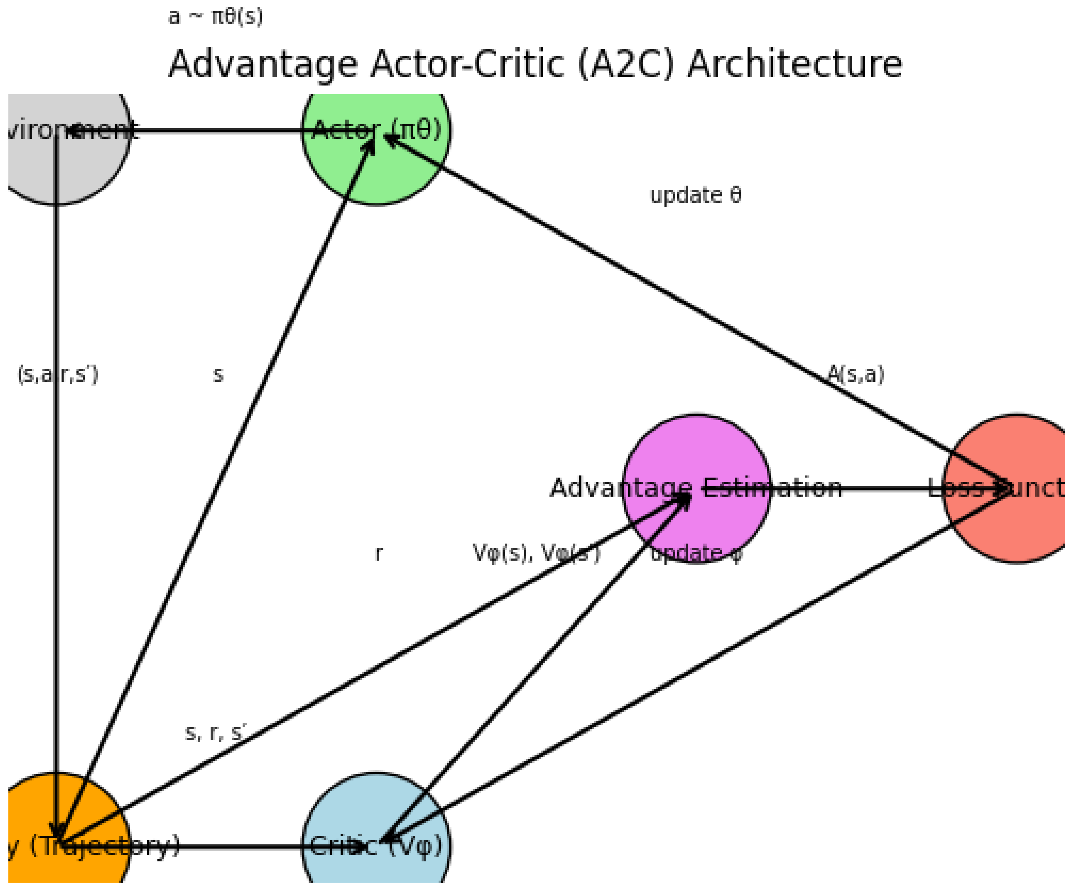
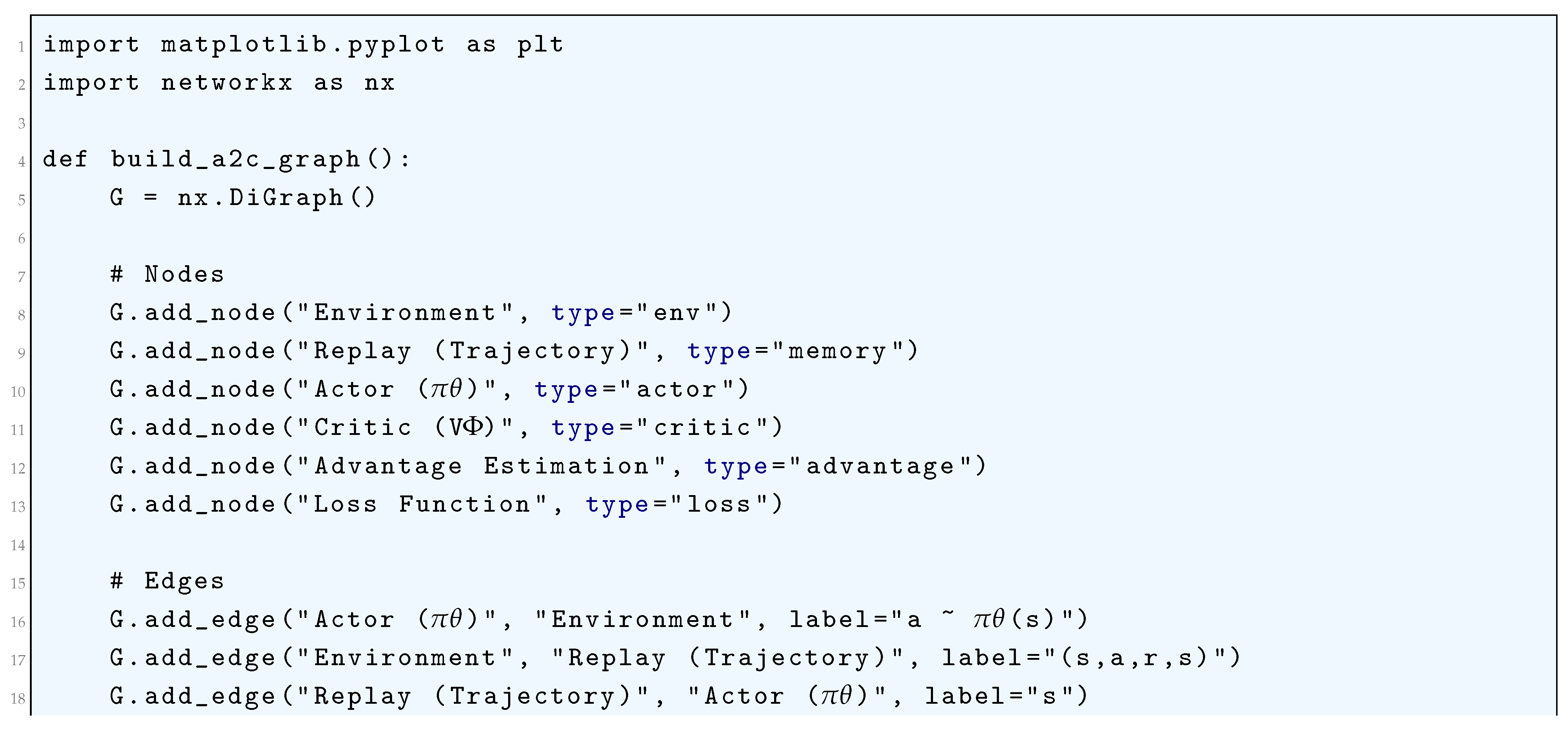
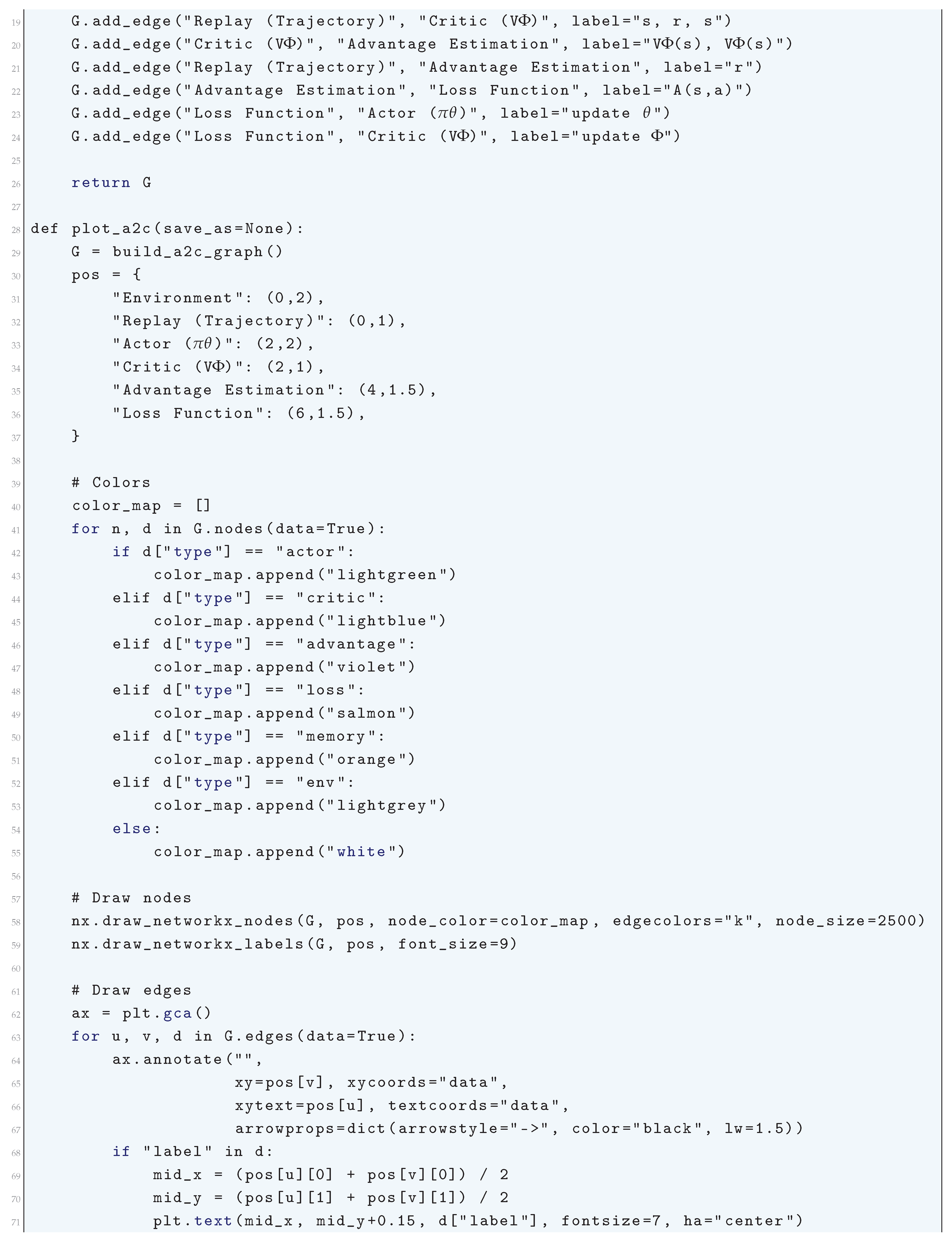
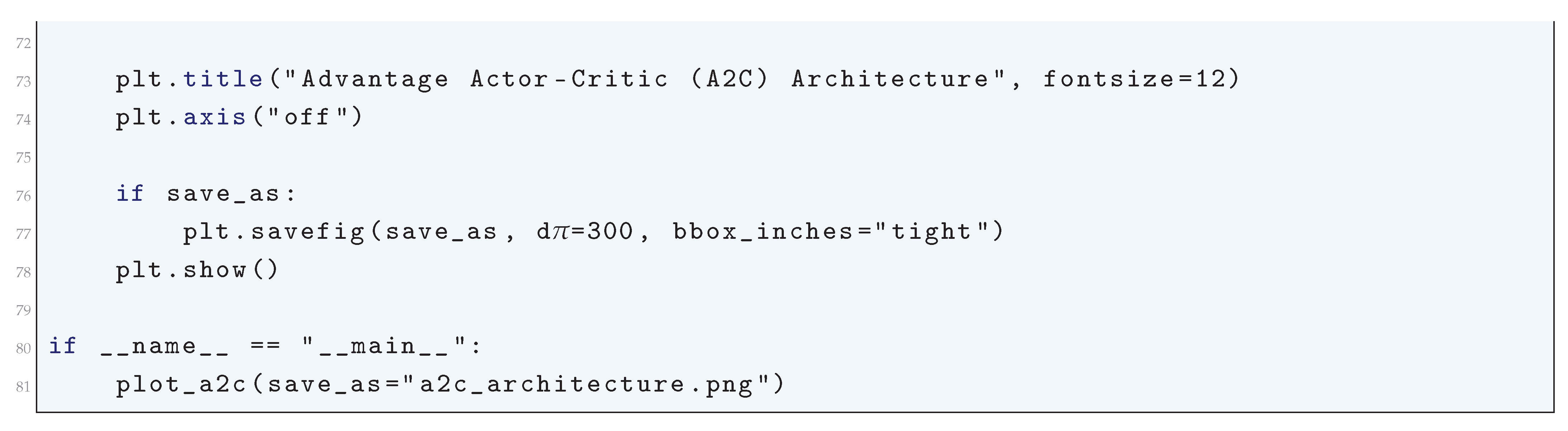
16.4.6.5 Deep Deterministic Policy Gradient
16.4.6.5.1 Literature Review of Deep Deterministic Policy Gradient
Deep Deterministic Policy Gradient (DDPG) has emerged as a fundamental algorithm in reinforcement learning (RL) for continuous action spaces, building upon deterministic policy gradients and deep Q-learning. The pioneering work by Lillicrap et al. (2015) [895] introduced the DDPG framework, integrating an actor-critic architecture with experience replay and target networks to stabilize training. This algorithm extends the Deterministic Policy Gradient (DPG) theorem from Silver et al. (2014) [851], which rigorously established that deterministic policy gradients can be computed with lower variance than their stochastic counterparts, making them particularly effective in high-dimensional continuous control tasks. While DDPG demonstrated its efficacy in simulated physics environments, subsequent research focused on addressing its limitations, particularly in off-policy learning, stability, and exploration. Cicek et al. (2021) [959] tackled the issue of off-policy correction by introducing Batch Prioritized Experience Replay, a technique that prioritizes data points based on their likelihood of being generated by the current policy. This enhancement improved sample efficiency by reducing policy divergence during updates, a critical challenge in off-policy deep RL methods.
Building upon these foundational ideas, Han et al. (2021) [960] proposed the Regularly Updated Deterministic (RUD) Policy Gradient Algorithm, which introduced a structured update mechanism to mitigate overestimation bias and variance in Q-value estimates. This was further refined by Pan et al. (2020) [961] in the Softmax Deep Double Deterministic Policy Gradient (SD3) method, which incorporated a Boltzmann softmax operator to smooth the optimization landscape and combat overestimation errors, leading to more reliable policy convergence. Addressing another major weakness of DDPG—exploration inefficiency—Luck et al. (2019) [962] proposed an approach that integrates latent trajectory optimization, where model-based trajectory estimation improves exploration in sparse-reward settings. Their work demonstrated that combining deep RL with latent variable models leads to improved generalization and efficiency in complex, high-dimensional environments. The practical applications of DDPG have also been expanded, with Dong et al. (2023) [963] developing an enhanced version for robotic arm control by integrating adaptive reward shaping and improved experience replay, yielding superior performance in dexterous manipulation tasks.
Beyond robotics, DDPG has been successfully applied in autonomous navigation and medical decision-making. Jesus et al. (2019) [964] extended the DDPG framework to mobile robot navigation, demonstrating its effectiveness in dynamic obstacle-avoidance scenarios without the need for explicit localization or map-based planning. Their results highlight DDPG’s ability to learn control policies in real-world environments where stochastic disturbances pose significant challenges. In a different domain, Lin et al. (2023) [965] employed DDPG for personalized medicine dosing strategies, illustrating how reinforcement learning can optimize complex decision-making processes in healthcare. Their approach aimed to replicate expert medical decisions, showcasing the potential for RL-based models to revolutionize treatment protocols by adapting to patient-specific characteristics. Lastly, the work of Sumalatha et al. (2024) [966] provided a rigorous overview of the evolution, enhancements, and applications of DDPG, consolidating various algorithmic advancements and practical implementations across multiple fields.
Collectively, these contributions form a rigorous and multifaceted body of research that extends DDPG’s theoretical foundations, addresses its key limitations, and explores novel applications in diverse domains. The enhancements in off-policy correction, policy update mechanisms, and exploration strategies underscore the continuous evolution of deep reinforcement learning methods to achieve greater efficiency, stability, and real-world applicability. As research in deep RL progresses, the integration of DDPG with meta-learning, hierarchical RL, and model-based approaches is expected to further enhance its capabilities, opening new frontiers in both theoretical and applied reinforcement learning.
Table 50.
Summary of Contributions in Deep Deterministic Policy Gradient (DDPG) Research
| Authors & Year | Contribution & Key Improvements |
| Lillicrap et al. (2015) | Introduced Deep Deterministic Policy Gradient (DDPG), combining deterministic policy gradients with deep Q-learning in an actor-critic framework. Enabled off-policy learning for high-dimensional continuous action spaces, stabilized training using target networks and experience replay. |
| Silver et al. (2014) | Developed the deterministic policy gradient theorem, proving that deterministic policies yield lower variance gradients compared to stochastic policy gradients. Provided the theoretical foundation for DDPG, ensuring efficient learning in continuous control environments. |
| Cicek et al. (2021) | Proposed Batch Prioritized Experience Replay (BPER) to improve off-policy learning by prioritizing data points based on their likelihood of being generated by the current policy. This reduced policy divergence and improved sample efficiency. |
| Han et al. (2021) | Developed the Regularly Updated Deterministic (RUD) Policy Gradient Algorithm to mitigate Q-value overestimation bias and variance. Introduced a structured update mechanism that improved stability in policy learning. |
| Pan et al. (2020) | Introduced Softmax Deep Double Deterministic Policy Gradient (SD3), incorporating a Boltzmann softmax operator to smooth policy updates. This reduced overestimation errors in Q-learning and improved stability during training. |
| Luck et al. (2019) | Integrated latent trajectory optimization with DDPG to enhance exploration in sparse-reward environments. Improved exploration by leveraging model-based trajectory estimation, enabling better generalization in complex environments. |
| Dong et al. (2023) | Extended DDPG for robotic arm control by integrating adaptive reward shaping and improved experience replay mechanisms. Increased policy robustness and efficiency in real-world dexterous manipulation tasks. |
| Jesus et al. (2019) | Applied DDPG to autonomous mobile robot navigation, demonstrating its effectiveness in real-time obstacle avoidance. Showed that learning-based control could be achieved without explicit localization or map-based planning. |
| Lin et al. (2023) | Used DDPG for personalized medicine dosing strategies to optimize treatment decisions. Demonstrated reinforcement learning’s capability in healthcare applications by personalizing medical treatment plans based on patient-specific characteristics. |
| Sumalatha et al. (2024) | Provided a comprehensive survey of DDPG advancements, consolidating various algorithmic improvements and practical applications across multiple domains. Analyzed the evolution of DDPG and its role in real-world implementations. |
16.4.6.5.2 Recent Literature Review of Deep Deterministic Policy Gradient
Deep Deterministic Policy Gradient (DDPG) has demonstrated significant advancements in diverse domains, particularly in optimizing resource allocation, decision-making, and control systems across vehicular networks, robotics, and UAV coordination. Recent studies have leveraged DDPG and its variations, such as Twin Delayed DDPG (TD3) and Multi-Agent Deep Deterministic Policy Gradient (MADDPG), to enhance performance in complex, real-time environments. For instance, in vehicular edge computing networks, Yang et al. (2025) [967] proposed a hierarchical optimization framework integrating DDPG to optimize driving mode selection and resource allocation, significantly reducing latency and improving efficiency. Similarly, Jamshidiha and Pourahmadi (2025) incorporated DDPG into a traffic-aware graph neural network for cellular networks, demonstrating improved user association and network adaptability. Furthermore, Tian et al. (2025) [968] introduced a Multi-State Iteration DDPG (SIDDPG) for the Internet of Vehicles (IoV), optimizing offloading strategies to minimize delays and energy consumption. These studies collectively highlight DDPG’s ability to dynamically optimize decision-making processes in vehicular and communication networks, ensuring enhanced network performance and resource utilization.
In addition to vehicular networks, DDPG has been extensively applied in robotics, UAV coordination, and cloud-edge computing. Raei et al. (2025) [920] introduced a DDPG-based reinforcement learning framework for non-prehensile robotic manipulation, demonstrating superior efficiency in dynamic control environments. In another application, Chen et al. (2025) [969] proposed a UAV-based computation offloading system utilizing DDPG, which optimizes task scheduling in cloud-edge collaborative environments, reducing latency and enhancing computational efficiency. Moreover, Ting-Ting et al. (2025) [921] developed a MADDPG-based approach for UAV clusters, ensuring robust decision-making under communication constraints. These studies illustrate DDPG’s adaptability to real-time, multi-agent environments, allowing for optimized coordination and resource management in robotics and aerial systems. By integrating reinforcement learning with real-world constraints, these approaches have successfully enhanced operational efficiency in autonomous systems.
Furthermore, advancements in DDPG have facilitated its application in emerging network and cloud computing paradigms. Deng et al. (2025) [970] expanded DDPG into a multi-agent reinforcement learning paradigm for non-terrestrial networks, enabling distributed coordination in satellite communications. Similarly, Anwar and Akber (2025) [903] incorporated MADDPG into structural engineering, optimizing building resilience by considering utility interactions under extreme conditions. Additionally, Zhang et al. (2025) [971] employed TD3 for multi-vehicle and multi-edge resource orchestration, optimizing computational tasks and minimizing system delays. These studies highlight the robustness of DDPG in optimizing decision-making processes across distributed networks, structural systems, and multi-agent interactions. By addressing dynamic, high-dimensional control problems, DDPG and its extensions continue to drive innovations in artificial intelligence and engineering.
In conclusion, the reviewed studies establish DDPG as a versatile and powerful reinforcement learning technique capable of handling continuous action-space optimization in diverse domains. From vehicular edge computing and UAV-based coordination to robotics and cloud-edge resource management, DDPG has demonstrated remarkable efficiency in optimizing real-time decision-making. With further advancements in multi-agent learning, federated reinforcement learning, and adaptive policy optimization, DDPG is poised to remain at the forefront of artificial intelligence research, revolutionizing complex control and resource allocation problems across various industries.
| Study | Contribution |
| Yang et al. (2025) | Introduced a three-stage hierarchical optimization framework (3SHO) where DDPG optimizes resource allocation, improving efficiency in vehicular networks. |
| Jamshidiha and Pourahmadi (2025) | Employed DDPG within a traffic-aware graph neural network to optimize user association, enhancing network adaptability in cellular networks. |
| Tian et al. (2025) | Developed Multi-State Iteration DDPG (SIDDPG) to optimize task partitioning and reduce latency and energy consumption in Internet of Vehicles (IoV). |
| Saad et al. (2025) | Applied Twin Delayed DDPG (TD3) for edge server selection in 5G-enabled industrial applications, minimizing computation delays. |
| Deng et al. (2025) | Proposed a Multi-Agent DDPG (MADDPG) for satellite communication networks, improving distributed coordination in non-terrestrial networks. |
| Raei et al. (2025) | Designed a DDPG-based reinforcement learning framework for robotic manipulation through sliding, improving control efficiency. |
| Ting-Ting et al. (2025) | Developed MADDPG with inter-agent communication for UAV clusters under constrained communication environments. |
| Zhang et al. (2025) | Utilized TD3 to optimize multi-vehicle and multi-edge computing resource allocation, reducing system delays in vehicular edge computing. |
| Chen et al. (2025) | Integrated DDPG into UAV-based computation offloading to improve task scheduling and computational efficiency in cloud-edge collaborative computing. |
| Anwar and Akber (2025) | Applied MADDPG to enhance building resilience through multi-agent reinforcement learning, optimizing utility interactions in structural engineering. |
16.4.6.5.3 Mathematical Analysis of Deep Deterministic Policy Gradient
Deep Deterministic Policy Gradient (DDPG) is a mathematically rigorous reinforcement learning (RL) algorithm that extends the classical Deterministic Policy Gradient (DPG) method to high-dimensional continuous action spaces by incorporating function approximators, particularly deep neural networks, to estimate both the policy and the value function. The algorithm is formulated within the framework of an infinite-horizon Markov Decision Process (MDP) characterized by a state space , an action space , a state transition probability distribution , a reward function , and a discount factor .
The agent’s objective is to learn a policy that maximizes the expected cumulative reward, given by the return function
The action-value function, or Q-function, is defined as the expected return starting from a state s and taking an action a, while following policy :
The Bellman equation for the Q-function under an optimal policy satisfies
Unlike traditional Q-learning approaches, which solve for discrete action spaces by iterating over all possible actions, DDPG employs an actor-critic architecture where the actor is a deterministic policy parameterized by that maps states directly to actions:
The critic function approximates the true Q-function and is parameterized by . The optimal policy parameters are obtained by maximizing the Q-value under the policy:
The deterministic policy gradient theorem states that the gradient of the expected return with respect to the policy parameters is
The Q-function is learned via the Bellman equation, leading to the following loss function for the critic:
where the target y is computed using a target Q-network and a target policy network :
To stabilize training, DDPG employs two techniques: (1) target networks, which are slow-moving versions of the policy and value networks, updated with soft updates
where ; and (2) an experience replay buffer D, where past transitions are stored and randomly sampled for training, breaking correlations between consecutive updates and improving sample efficiency.
16.4.6.5.4 Python Code to Generate Figure 189
DDPG is an actor–critic, off-policy RL algorithm with:
- Actor (policy network) outputs continuous actions.
- Critic (Q-network) evaluates .
- Target networks stabilize learning.
- Replay buffer stores transitions.
- Environment generates experience.
The Python code below produces the Figure 189 illustrating the Deep Deterministic Policy Gradient.
Figure 189.
Architecture of the Deep Deterministic Policy Gradient (DDPG) algorithm. The actor network (green) outputs continuous actions. The environment (gray) produces transitions, which are stored in a replay buffer (orange). The critic (blue) and target networks (violet) evaluate Q-values and compute target values. The loss function (red) updates both actor and critic networks via policy gradients and temporal-difference learning
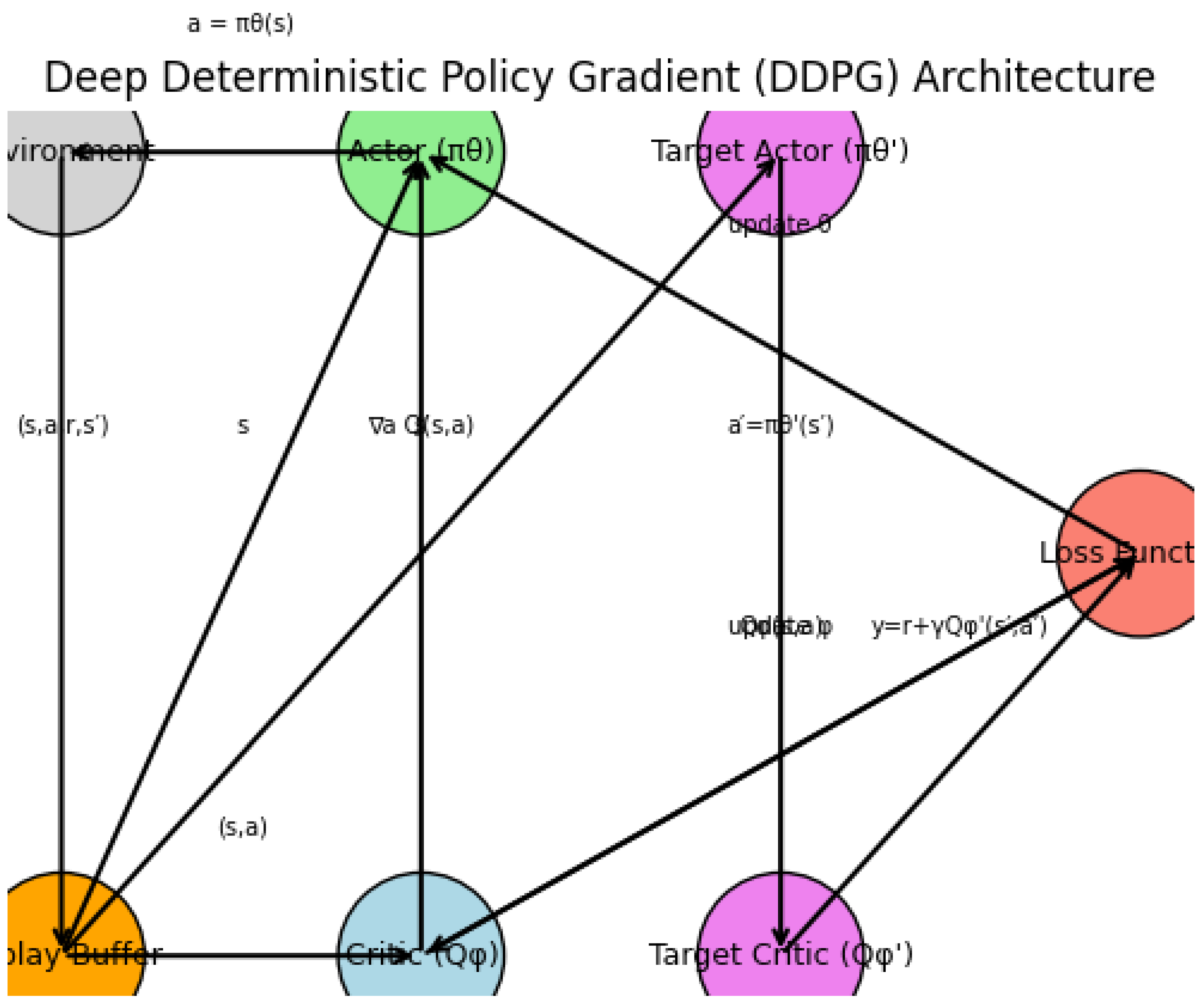
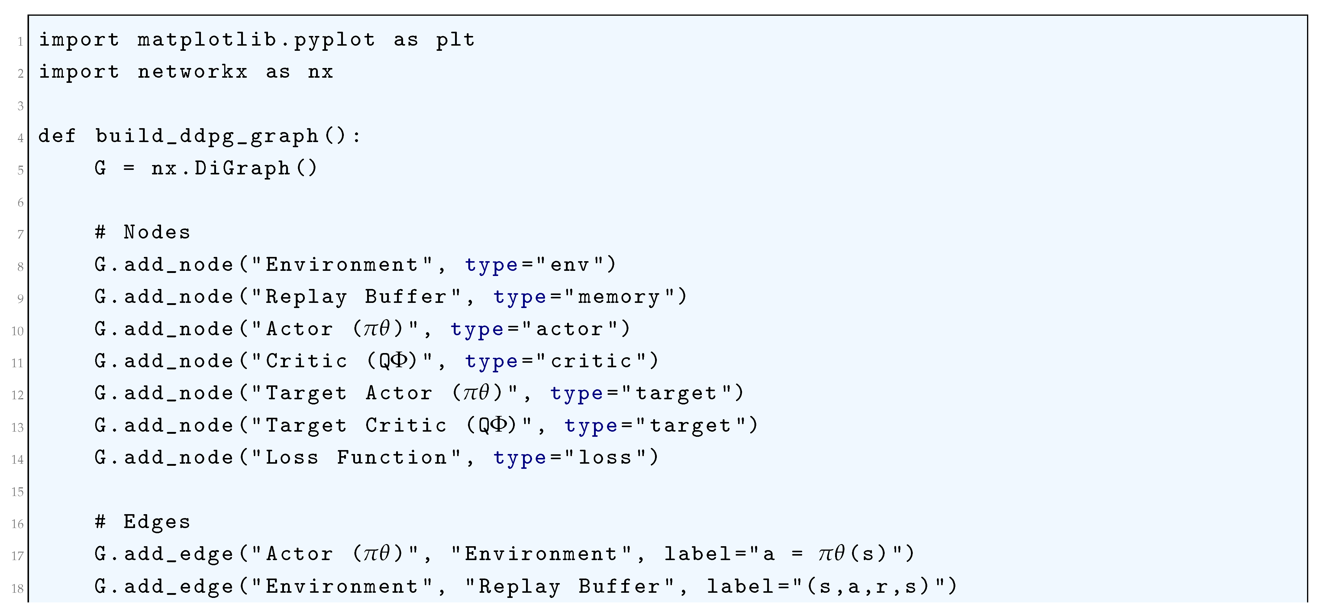
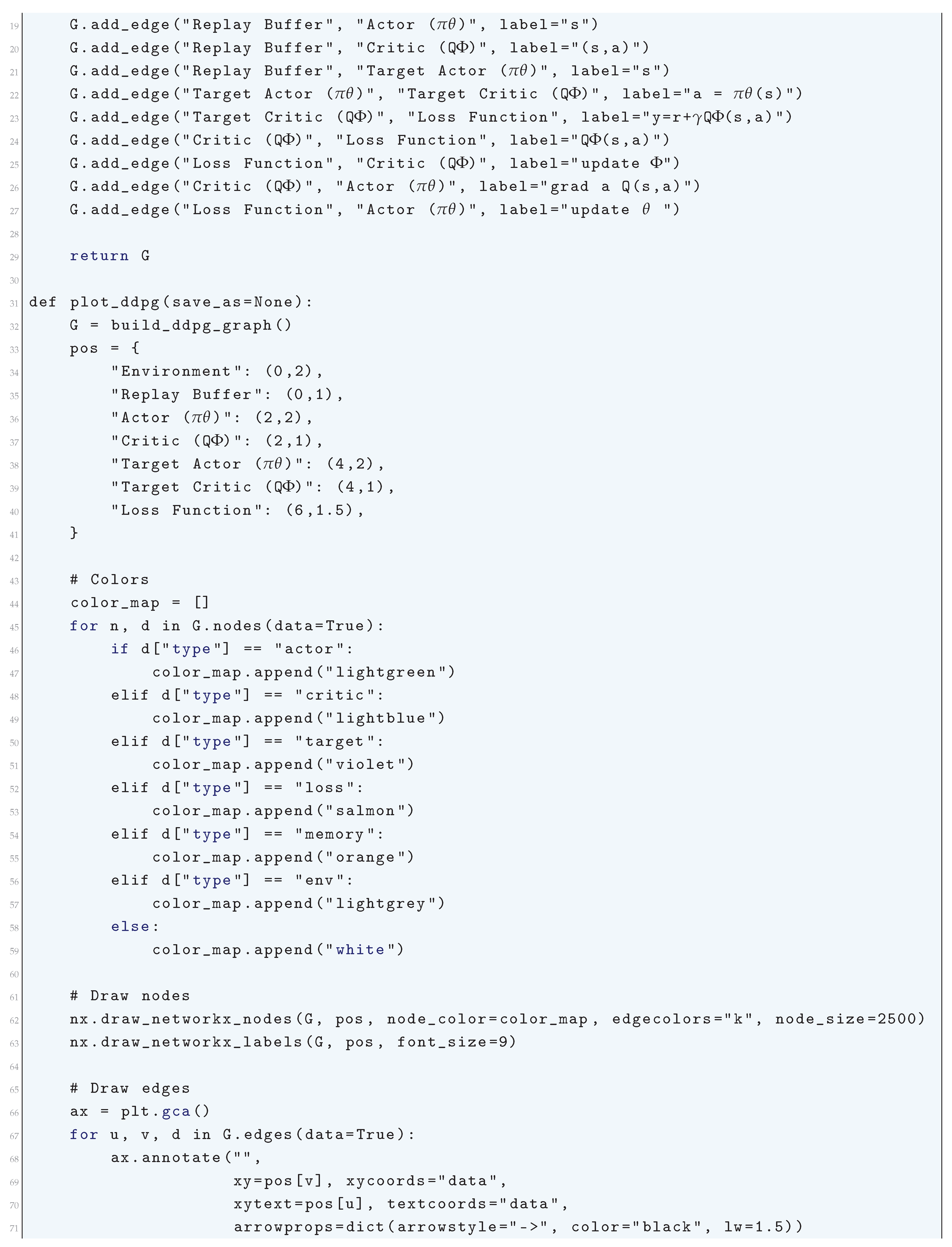
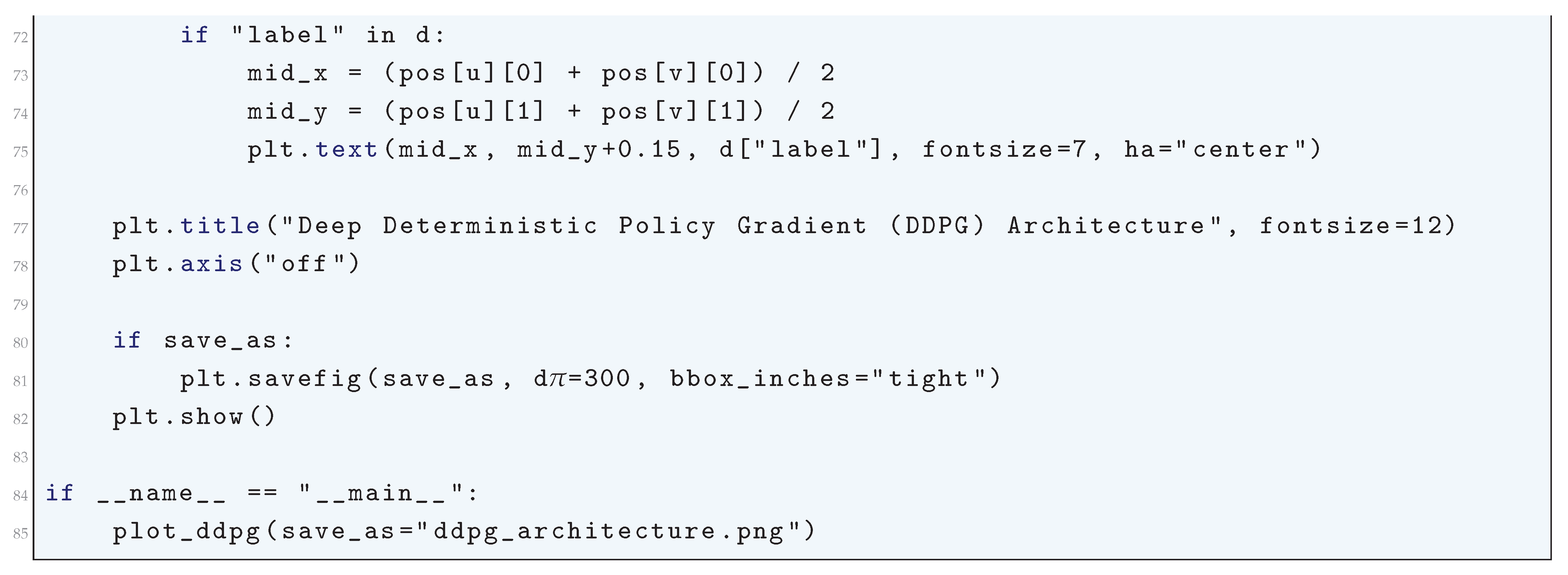
16.4.6.6 Proximal Policy Optimization
16.4.6.6.1 Literature Review of Proximal Policy Optimization
Proximal Policy Optimization (PPO) has become one of the most widely used policy gradient methods due to its balance between computational efficiency and stable performance. Schulman et al. (2017) laid the theoretical foundation for PPO by introducing a first-order optimization technique that constrains policy updates through a clipped surrogate objective, ensuring stable and reliable learning without requiring the complex second-order optimization steps of Trust Region Policy Optimization (TRPO). Following its introduction, researchers identified several critical implementation details that significantly impact PPO’s performance. Huang and Dossa (2022) compiled a comprehensive list of 37 key implementation details, highlighting often-overlooked hyperparameter choices, network architectures, and training strategies necessary for PPO to perform consistently across different tasks. These insights provided a crucial guideline for practitioners and researchers to reproduce PPO’s results accurately, preventing performance discrepancies arising from subtle implementation variations.
Several studies have proposed refinements to PPO’s clipping mechanism to enhance training stability and sample efficiency. Zhang et al. (2023) addressed the issue of fixed clipping bounds by introducing a dynamic adjustment mechanism that utilizes task-specific feedback, thereby ensuring that policy updates remain within an optimal range. This adaptation mitigates the issue of overly aggressive policy updates in early training stages while preventing excessive conservatism in later stages. Similarly, Zhang et al. (2020) proposed an alternative dynamic clipping strategy to fine-tune the trade-off between exploration and exploitation, further improving PPO’s adaptability. Another notable contribution in this domain is Kobayashi’s (2022) introduction of an adaptive threshold for PPO using the symmetric relative density ratio, which optimally adjusts the clipping bound based on the scale of the policy update error. This method improves training stability and ensures a more theoretically grounded approach to threshold selection. Kobayashi (2020) extended this idea by formulating PPO using relative Pearson divergence, which provides an intuitive and principled way to constrain policy updates, thereby achieving smoother and more stable training dynamics.
Beyond single-agent reinforcement learning, PPO has also been extended to multi-agent systems. Piao and Zhuo (2021) introduced Coordinated Proximal Policy Optimization (CoPPO), which adapts step sizes dynamically for multiple interacting agents, mitigating instability issues caused by independent updates in decentralized training settings. The coordinated adaptation mechanism significantly enhances PPO’s applicability in complex environments where multiple agents must learn simultaneously while maintaining stability in learning dynamics. Additionally, Wang et al. (2019) proposed Truly Proximal Policy Optimization (TPPO), which integrates a trust region constraint directly into the objective function, thereby ensuring that updates remain within a theoretically justified range and reducing the likelihood of catastrophic policy collapse. These modifications further reinforced PPO’s theoretical robustness by explicitly incorporating policy divergence constraints.
Finally, a broader perspective on PPO’s reliability was provided by Henderson et al. (2018), who critically examined deep reinforcement learning methodologies and demonstrated that performance metrics in literature are highly sensitive to hyperparameter tuning and implementation details. Their findings underscored the necessity of rigorous benchmarking and reproducibility standards to ensure that performance improvements claimed by various PPO enhancements are not merely the result of uncontrolled hyperparameter tuning. Collectively, these contributions showcase the continuous evolution of PPO, from its theoretical foundation to practical improvements in policy update mechanisms, stability guarantees, and applicability in multi-agent reinforcement learning. They also highlight the importance of principled algorithm design and robust evaluation methodologies to advance reinforcement learning research in a scientifically rigorous manner.
| Reference | Contribution |
| Schulman et al. (2017) | Introduced Proximal Policy Optimization (PPO), a first-order policy gradient method that balances stability and efficiency. PPO replaces the trust region constraint in TRPO with a clipped surrogate objective, simplifying implementation while maintaining strong empirical performance across various reinforcement learning tasks. |
| Huang and Dossa (2022) | Provided a comprehensive checklist of 37 crucial implementation details necessary for reproducing PPO’s reported performance. This work highlighted the impact of hyperparameter choices, architectural considerations, and training strategies on PPO’s consistency and reliability. |
| Zhang et al. (2023) | Proposed a dynamic clipping strategy where the clipping threshold adapts based on task feedback, ensuring optimal constraint selection for policy updates. This method improves training stability and sample efficiency while addressing PPO’s sensitivity to fixed clipping bounds. |
| Zhang et al. (2020) | Developed an exploration-enhancing variant of PPO that incorporates uncertainty estimation. Their approach improves sample efficiency by encouraging exploration in regions of high uncertainty, particularly in continuous control tasks. |
| Kobayashi (2022) | Introduced a threshold adaptation mechanism for PPO using the symmetric relative density ratio, leading to a more theoretically grounded method for selecting the clipping bound. This modification enhances stability and improves policy update efficiency. |
| Kobayashi (2020) | Formulated PPO using relative Pearson divergence, providing a principled policy divergence constraint that ensures smoother and more stable training updates, improving theoretical soundness. |
| Piao and Zhuo (2021) | Extended PPO to multi-agent reinforcement learning by introducing Coordinated Proximal Policy Optimization (CoPPO), which adapts step sizes dynamically for multiple interacting agents. This approach improves training stability and performance in decentralized multi-agent environments. |
| Zhang and Wang (2020) | Proposed a dynamic clipping bound method that adjusts the threshold throughout training, further refining the balance between exploration and exploitation in PPO-based learning. |
| Wang et al. (2019) | Introduced Truly Proximal Policy Optimization (TPPO), which explicitly incorporates a trust region constraint into PPO’s objective function, leading to more reliable and theoretically grounded policy updates. |
| Henderson et al. (2018) | Critically examined the reproducibility of deep reinforcement learning algorithms, including PPO. The study demonstrated the sensitivity of performance metrics to hyperparameter tuning and implementation details, emphasizing the need for rigorous benchmarking and standardization in reinforcement learning research. |
16.4.6.6.2 Recent Literature Review of Proximal Policy Optimization
Proximal Policy Optimization (PPO) has emerged as a robust reinforcement learning algorithm with wide-ranging applications across multiple domains, from space exploration to autonomous robotics and networking optimization. One of its notable implementations is in interplanetary trajectory design, where PPO is leveraged to optimize orbital maneuvers, ensuring efficient fuel management and trajectory planning under stringent mission constraints (Cuéllar et al., 2024) [972]. This showcases PPO’s ability to handle high-dimensional decision-making problems. Similarly, in autonomous underwater robotics, PPO is employed for three-dimensional trajectory planning by integrating fluid dynamics-based motion strategies, allowing underwater vehicles to adapt to dynamic marine environments and external perturbations (Liu et al., 2025) [973]. The adaptability of PPO in handling complex physical constraints further extends to humanoid robotics, where it enables fast multimodal gait learning, allowing bipedal robots to adjust walking patterns across varying terrains through reinforcement-based self-learning mechanisms (Figueroa et al., 2025) [974]. These applications underscore the strength of PPO in real-world motion planning and adaptive control.
In networking and communication systems, PPO has demonstrated its efficacy in cognitive radio networks and edge computing. For instance, a Lyapunov-guided PPO-based resource allocation model optimizes spectrum sharing and power distribution in dynamic radio environments, reducing latency and maximizing throughput (Xu et al., 2025) [975]. Similarly, vehicular networks benefit from PPO-driven computation offloading, where the algorithm efficiently schedules tasks between cloud and edge nodes to enhance latency-sensitive applications (Mustafa et al., 2025) [917]. PPO has also been employed in anti-jamming wireless communication to dynamically allocate spectrum resources in adversarial settings, ensuring robust and resilient connectivity (Li et al., 2025) [976]. These applications illustrate how PPO enhances real-time decision-making in complex, distributed systems that require efficient task execution and resource utilization.
Beyond robotics and communication, PPO has been instrumental in optimizing industrial processes and energy systems. In cloud computing, PPO has been integrated with graph neural networks (GNNs) to optimize dynamic workflow scheduling, reducing both computational overhead and energy consumption in large-scale cloud environments (Chandrasiri and Meedeniya, 2025) [977]. Moreover, a smart building energy management system leverages PPO to dynamically regulate heating, ventilation, and air conditioning (HVAC) operations, significantly improving carbon efficiency (Wu and Xie, 2025) [979]. In the manufacturing sector, Guan et al. (2025) [980] proposed a multi-agent PPO-based approach for real-time production scheduling and AGV selection, ensuring just-in-time logistics and maximizing supply chain efficiency. These implementations highlight PPO’s impact on autonomous decision-making for sustainability and operational efficiency.
Finally, PPO’s utility in decision-making under uncertainty is evident in financial markets and transportation systems. In stock portfolio management, PPO is integrated with reinforcement-based market simulations to optimize trade execution, balancing risk and return in volatile environments (Zhang et al., 2025) [981]. Additionally, in autonomous vehicle trajectory planning, PPO is combined with control barrier function techniques to ensure collision-free navigation in high-speed driving scenarios, refining behavior planning strategies at complex intersections (Zhang et al., 2025) [982]. These cases demonstrate PPO’s capability in learning optimal policies in dynamic, stochastic environments, making it an invaluable tool for real-time AI decision-making. Across all these domains, PPO continues to drive innovation by balancing exploration and exploitation, allowing intelligent systems to adapt to ever-changing real-world constraints efficiently.
| Author(s) & Year | Contribution |
| Cuéllar et al., 2024 | Uses PPO for optimizing interplanetary trajectory design, ensuring efficient orbital maneuvers with fuel management optimization. |
| Guan et al., 2025 | Integrates PPO with a transformer-based attention mechanism for vehicle routing, improving convergence and efficiency. |
| Wu & Xie, 2025 | Proposes PPO for optimizing HVAC energy efficiency in smart buildings, significantly reducing carbon footprint. |
| Chandrasiri & Meedeniya, 2025 | Combines PPO with Graph Neural Networks to optimize cloud workflow scheduling, reducing latency and energy use. |
| Liu et al., 2025 | Employs PPO to optimize real-time navigation for underwater robots, adapting to environmental disturbances. |
| Mustafa et al., 2025 | Uses PPO for dynamic task offloading in edge-assisted vehicular networks, enhancing real-time resource management. |
| Figueroa et al., 2025 | Applies PPO for humanoid robot gait adaptation, enabling robots to walk efficiently across different terrains. |
| Xu et al., 2025 | Develops a PPO-based Lyapunov-guided model for optimizing resource allocation in cognitive radio networks. |
| Bukhari et al., 2025 | Integrates PPO with causal learning for natural language-based robotic control, improving adaptability in robotics. |
| Dai et al., 2025 | Utilizes PPO with control barrier functions for autonomous vehicle trajectory planning, ensuring safe and efficient merging. |
16.4.6.6.3 Mathematical Analysis of Proximal Policy Optimization
Proximal Policy Optimization (PPO) is a policy gradient method used in reinforcement learning that seeks to improve the stability and efficiency of policy updates while maintaining sample efficiency. Given a Markov Decision Process (MDP) defined by the tuple , where is the state space, is the action space, represents the transition probabilities, is the reward function, and is the discount factor, PPO aims to find an optimal policy parameterized by , maximizing the expected cumulative discounted reward. The objective function for policy optimization is given by the expected advantage-weighted likelihood ratio:
where is the advantage function that quantifies how much better an action is compared to the expected value of the state under the old policy. To prevent overly large updates that can lead to instability, PPO employs a clipped surrogate objective:
where the importance sampling ratio is defined as
and is a hyperparameter that controls how much the new policy can deviate from the old policy. The clipping mechanism ensures that if the policy update step would lead to a large change in action probability, the advantage function is modified to prevent large updates, thereby stabilizing training. The clipped term can be rewritten as
This formulation ensures that the policy update is constrained within a predefined trust region without requiring explicit second-order optimization methods, unlike Trust Region Policy Optimization (TRPO).
Additionally, PPO often includes a value function term to reduce variance while maintaining unbiased gradient estimates. The value loss function is given by
where is the learned state-value function and is the estimated target value function computed from bootstrapped returns, typically using Generalized Advantage Estimation (GAE):
where the return is
and the advantage function is estimated using GAE:
with the temporal difference residual
where is a smoothing parameter that controls the bias-variance tradeoff. The final PPO objective function combines the clipped surrogate loss, value function loss, and an entropy bonus to encourage exploration:
where and are hyperparameters and is the entropy term given by
which ensures policy exploration by discouraging premature convergence to deterministic policies. The policy updates are performed iteratively using stochastic gradient ascent with Adam optimizer:
where is the learning rate. Since PPO is an on-policy method, experience data is collected under the current policy and discarded after updates. The training follows a batch-wise paradigm where sampled trajectories are used to update the policy over multiple epochs. By balancing exploration, sample efficiency, and stability, PPO achieves robust policy optimization across diverse reinforcement learning tasks.
16.4.6.6.4 Python Code to Generate Figure 190
Proximal Policy Optimization (PPO) is one of the most widely used policy gradient algorithms. To visualize PPO, a good diagram shows the data flow between:
- Environment → generates transitions Policy (Actor) → produces actions from states.
- Value Function (Critic) → estimates state values
- Advantage Estimator → computes using rewards and values.
- Clipped Objective → updates the policy with constraints to prevent large steps.
- Replay/Trajectory Buffer → stores collected rollouts.
The Python code below produces the Figure 190 illustrating the Proximal Policy Optimization (PPO).
Figure 190.
Architecture of the Proximal Policy Optimization (PPO) algorithm: The actor (green) outputs actions, interacting with the environment (gray). Rollouts are stored in a trajectory buffer (orange). The critic (blue) estimates value functions, and the advantage estimator (violet) computes advantages . The clipped surrogate objective (red) combines policy ratios and advantages to update the actor stably
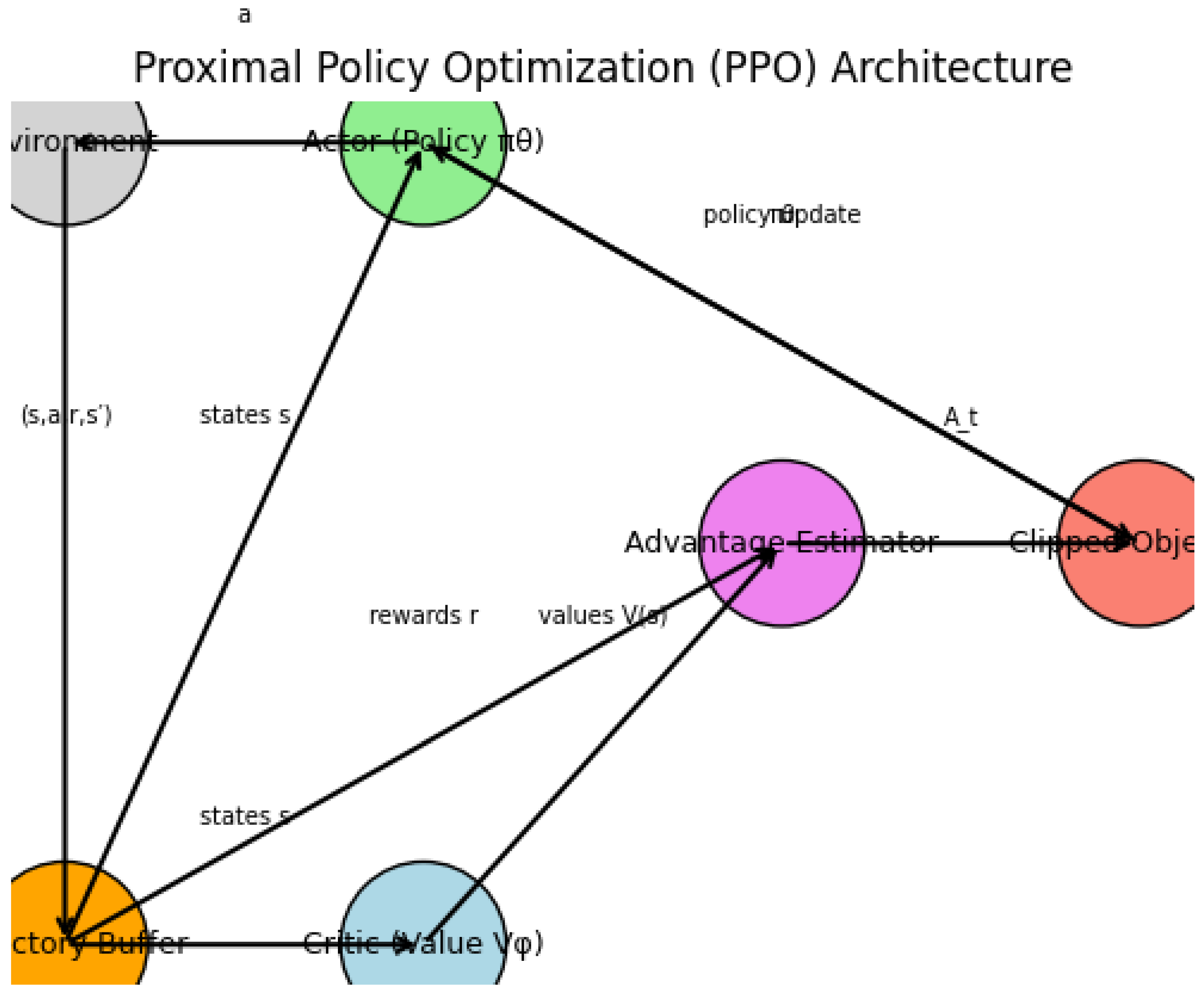
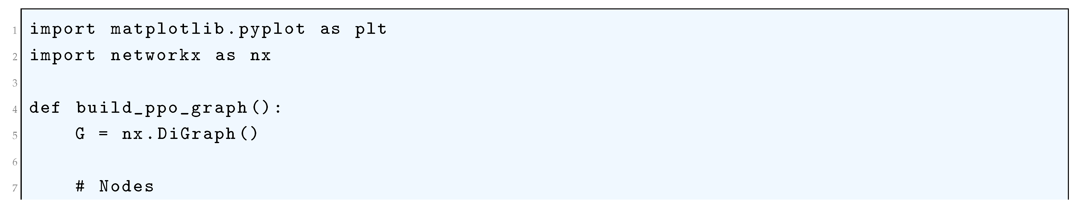
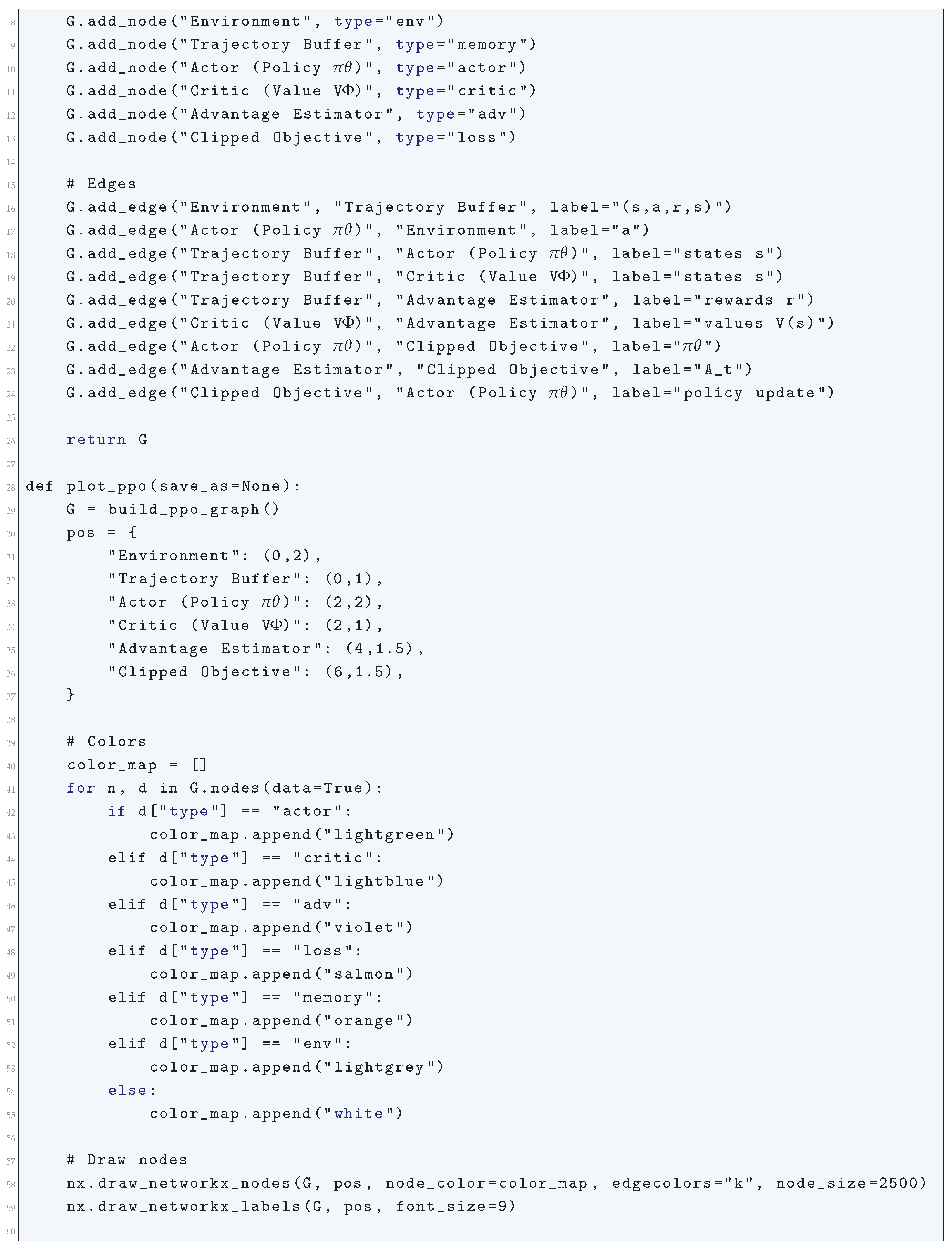
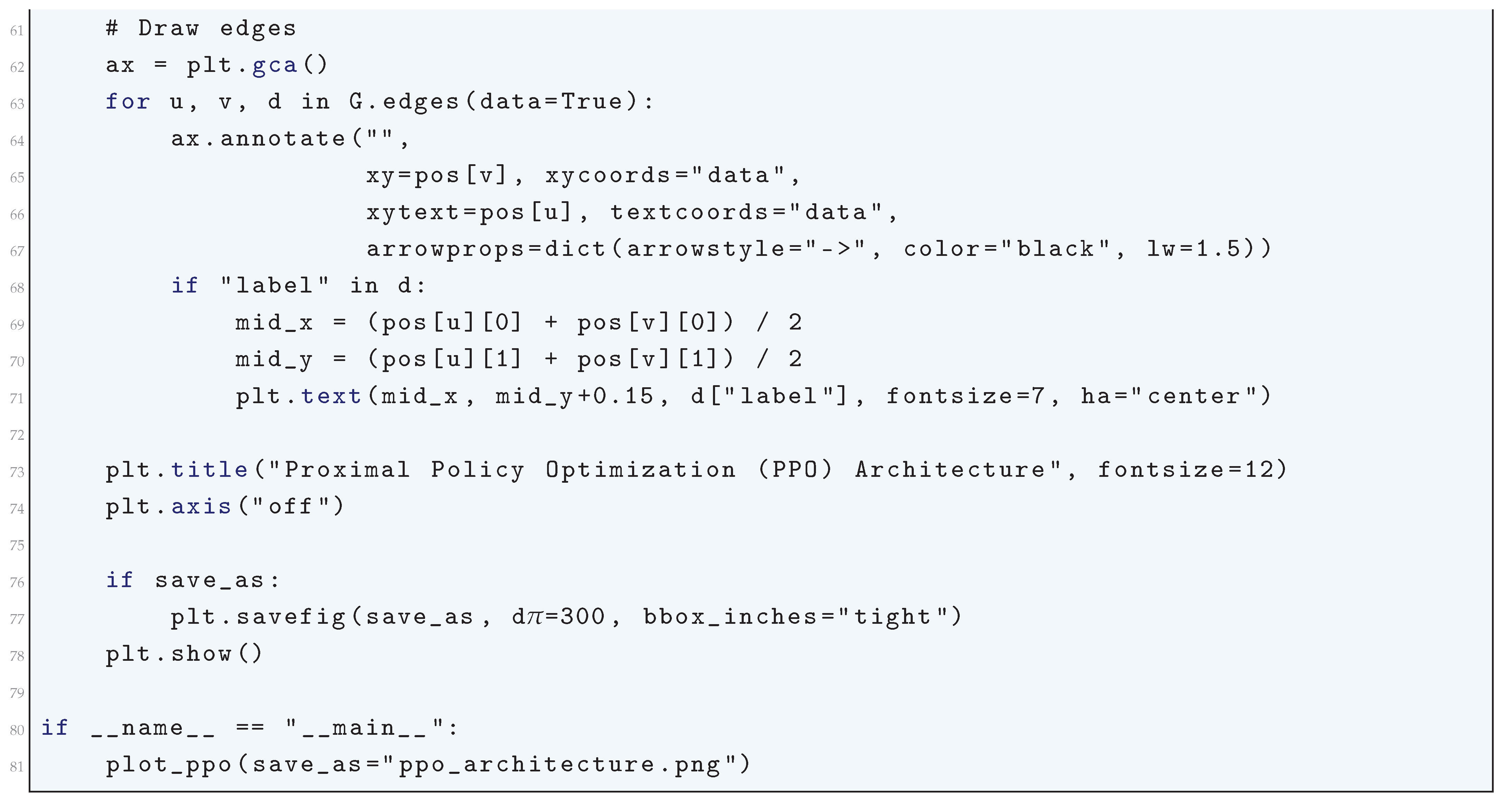
16.4.6.7 Soft Actor-Critic (SAC) Algorithm
16.4.6.7.1 Literature Review of Soft Actor-Critic (SAC) Algorithm
The Soft Actor-Critic (SAC) algorithm, originally proposed by Haarnoja et al. (2018), introduced a novel framework that integrates the maximum entropy principle with off-policy reinforcement learning, significantly enhancing sample efficiency, stability, and robustness of policy learning. The key contribution of SAC lies in its entropy-regularized objective, which encourages policies to not only maximize expected returns but also maintain high entropy, ensuring effective exploration and better generalization across unseen states. This approach was further refined in Haarnoja et al. (2019), where an automatic temperature tuning mechanism was introduced to dynamically balance the trade-off between exploration and exploitation, alleviating the need for exhaustive hyperparameter tuning. These developments enabled SAC to outperform existing algorithms such as Deep Deterministic Policy Gradient (DDPG) and Twin Delayed DDPG (TD3) on a variety of continuous control benchmarks, demonstrating superior performance in both sample efficiency and policy robustness.
Several extensions of SAC have been proposed to address specific challenges in robotics, autonomous navigation, and uncertainty estimation. Wu et al. (2023) applied SAC to LiDAR-based robot navigation, where the algorithm was adapted to dynamic obstacle avoidance scenarios, showing improved training efficiency and navigation success rates. Similarly, Hossain et al. (2022) introduced an inhibitory network-based modification to SAC, designed to accelerate the retraining of UAV controllers, thereby enhancing adaptability in fast-changing environments. Another significant development came from Ishfaq et al. (2025), who introduced Langevin Soft Actor-Critic (LSAC), integrating Thompson sampling with distributional Langevin Monte Carlo updates to improve uncertainty estimation and exploration efficiency. These contributions reflect ongoing efforts to tailor SAC for real-world applications where stability and robustness are paramount.
Further theoretical advancements have sought to refine the critic network and improve value estimation in SAC. Verma et al. (2023) proposed the Soft Actor Retrospective Critic (SARC), which introduced an additional retrospective loss term for the critic network, accelerating convergence and stabilizing training dynamics. Addressing concerns regarding approximation errors, Tasdighi et al. (2023) introduced PAC-Bayesian Soft Actor-Critic, which incorporates a PAC-Bayesian objective into the critic’s learning process, reducing uncertainty and improving sample efficiency. In a related effort, Duan (2021) proposed Distributional Soft Actor-Critic (DSAC), which learns a Gaussian distribution over stochastic returns, mitigating value overestimation errors commonly encountered in standard SAC implementations. These refinements collectively contribute to more reliable policy learning, especially in high-dimensional continuous control tasks.
Beyond algorithmic improvements, theoretical explanations and comparative studies have solidified SAC’s role as a benchmark reinforcement learning algorithm. The Papers with Code analysis provides a detailed breakdown of SAC’s fundamental principles, highlighting its superiority over traditional policy optimization methods due to its ability to capture multi-modal policy distributions. This is complemented by the in-depth analyses of Haarnoja et al., who emphasize the algorithm’s strengths in handling stochasticity while maintaining computational tractability. Taken together, these contributions establish SAC as one of the most powerful and widely adopted actor-critic methods in deep reinforcement learning, continuing to inspire further research in robotics, autonomous systems, and sample-efficient deep reinforcement learning.
| Authors (Year) | Contribution |
| Haarnoja et al. (2018) | Introduced Soft Actor-Critic (SAC), integrating the maximum entropy principle into reinforcement learning to enhance sample efficiency, stability, and policy robustness. SAC introduced an entropy-regularized objective, encouraging high-entropy policies for better exploration and generalization. |
| Haarnoja et al. (2019) | Developed an automatic temperature tuning mechanism for SAC, dynamically adjusting the entropy coefficient to balance exploration and exploitation. This improvement alleviates the need for manual hyperparameter tuning, leading to more adaptive learning. |
| Wu et al. (2023) | Applied SAC to LiDAR-based robot navigation, demonstrating its effectiveness in dynamic obstacle avoidance. The study showed improved training efficiency and higher navigation success rates, making SAC more viable for real-world robotic applications. |
| Hossain et al. (2022) | Proposed an inhibitory network-based modification to SAC for UAV control, enhancing adaptability and retraining speed in fast-changing environments. This modification allows SAC to better handle non-stationary reinforcement learning settings. |
| Ishfaq et al. (2025) | Introduced Langevin Soft Actor-Critic (LSAC), combining SAC with Thompson sampling and distributional Langevin Monte Carlo updates to improve uncertainty estimation and exploration efficiency. This modification leads to more robust decision-making under uncertainty. |
| Verma et al. (2023) | Developed the Soft Actor Retrospective Critic (SARC), incorporating a retrospective loss term in the critic network to accelerate convergence and stabilize training dynamics, improving sample efficiency in high-dimensional problems. |
| Tasdighi et al. (2023) | Introduced PAC-Bayesian Soft Actor-Critic, integrating a PAC-Bayesian objective into SAC’s critic network to reduce uncertainty and improve sample efficiency. This approach provides theoretical guarantees on policy performance. |
| Duan (2021) | Proposed Distributional Soft Actor-Critic (DSAC), learning a Gaussian distribution over stochastic returns to mitigate value overestimation errors in standard SAC implementations. This leads to more reliable policy learning in continuous control tasks. |
| Papers with Code Analysis | Provided a comprehensive breakdown of SAC’s theoretical foundations, benchmarking its performance across various continuous control environments, and highlighting its superiority over traditional policy optimization methods. |
| Haarnoja et al. (Various Analyses) | Conducted in-depth studies on SAC’s ability to handle stochasticity, demonstrating its advantages in learning multi-modal policy distributions while maintaining computational efficiency. |
16.4.6.7.2 Recent Literature Review of Soft Actor-Critic (SAC) Algorithm
Soft Actor-Critic (SAC) has emerged as a powerful deep reinforcement learning algorithm, demonstrating remarkable adaptability across various domains such as autonomous systems, financial markets, industrial automation, and transportation. One significant application is in search and rescue operations, where SAC outperforms traditional reinforcement learning methods due to its entropy-regularized policy. Ewers et al. (2025) implement SAC alongside Proximal Policy Optimization (PPO) in a recurrent autoencoder-based deep reinforcement learning system, revealing SAC’s superiority in handling dynamic and uncertain environments. Similarly, in fluid dynamics, Yan et al. (2025) propose mutual information-based knowledge transfer learning (MIKT-SAC), enhancing SAC’s ability to generalize across domains for active flow control in bluff body flows, demonstrating significant improvements in cross-domain transferability. Another critical industrial application is seen in Industry 5.0, where Asmat et al. (2025) develop a Digital Twin (DT) framework integrated with SAC, enabling intelligent cyber-physical systems for adaptive industrial transitions. Moreover, SAC is extensively utilized in telecommunications, as highlighted by Chao and Jiao (2025), who leverage SAC for network spectrum resource allocation, optimizing spectrum usage in dynamic wireless environments.
Beyond industrial applications, SAC is also making strides in autonomous navigation and adversarial learning. Ma et al. (2025) introduce SIE-SAC, an advanced SAC-based learning mechanism for UAV navigation under adversarial conditions, specifically GPS/INS-integrated spoofing scenarios. The study underscores SAC’s capability to adapt and refine deception strategies, a crucial element in defensive aerospace applications. Additionally, SAC is being explored in financial markets, where Walia et al. (2025) integrate SAC with causal generative adversarial networks (GANs) and large language models (LLMs) for liquidity-aware bond yield prediction. This approach significantly enhances financial forecasting by leveraging reinforcement learning’s adaptability in complex, non-linear financial datasets. Lalor and Swishchuk (2025) further extend SAC’s financial applications by applying it to non-Markovian market-making, proving its efficiency in handling long-term dependencies and stochastic pricing models.
SAC’s utility is not limited to theoretical models but also extends into multi-agent cooperative learning and resource optimization. Zhang et al. (2025) propose a diffusion-based SAC framework for multi-UAV networks in the Metaverse, optimizing cooperative task allocation and resource distribution in edge-enabled virtual environments. Similarly, Zhao et al. (2025) apply SAC in energy management for hybrid storage systems in urban rail transit, enhancing the efficiency of traction power supply systems. This approach demonstrates SAC’s potential in sustainable energy applications, where efficient power distribution is paramount. In the automotive sector, Tresca et al. (2025) utilize SAC to design adaptive energy management strategies for hybrid electric vehicles, optimizing fuel efficiency and battery longevity by dynamically adjusting energy consumption based on real-time driving conditions.
Overall, SAC continues to revolutionize deep reinforcement learning across various domains by providing sample-efficient, entropy-regularized learning strategies that balance exploration and exploitation effectively. From autonomous navigation and cybersecurity to industrial optimization and sustainable energy systems, SAC’s ability to handle high-dimensional, complex decision-making problems ensures its widespread applicability. Whether applied in robotics, finance, or telecommunications, SAC demonstrates exceptional versatility, pushing the boundaries of intelligent decision-making in real-world systems.
| Authors (Year) | Contribution |
| Ewers et al. (2025) | Implement SAC and PPO in a recurrent autoencoder-based reinforcement learning framework for search and rescue operations, demonstrating SAC’s superior performance in dynamic and uncertain environments. |
| Yan et al. (2025) | Develop a mutual information-based knowledge transfer learning (MIKT-SAC) method to enhance SAC’s generalization across domains, improving active flow control in bluff body flows. |
| Asmat et al. (2025) | Propose a Digital Twin (DT) framework integrated with SAC to enable intelligent cyber-physical systems, facilitating the transition from Industry 4.0 to Industry 5.0. |
| Chao & Jiao (2025) | Apply SAC for network spectrum resource allocation, optimizing spectrum usage in dynamic wireless environments to enhance telecommunications efficiency. |
| Ma et al. (2025) | Introduce SIE-SAC, a novel reinforcement learning mechanism for UAV navigation in adversarial conditions, particularly in GPS/INS-integrated spoofing scenarios. |
| Walia et al. (2025) | Combine SAC with causal generative adversarial networks (GANs) and large language models (LLMs) to improve bond yield predictions and enhance financial forecasting. |
| Lalor & Swishchuk (2025) | Extend SAC to non-Markovian market-making, demonstrating its effectiveness in handling long-term dependencies and stochastic pricing models. |
| Zhang et al. (2025) | Propose a diffusion-based SAC framework for multi-UAV networks in the Metaverse, optimizing cooperative task allocation and resource distribution. |
| Zhao et al. (2025) | Utilize SAC for energy management in hybrid storage systems for urban rail transit, optimizing power distribution in traction power supply systems. |
| Tresca et al. (2025) | Apply SAC to develop adaptive energy management strategies for hybrid electric vehicles, enhancing fuel efficiency and battery longevity through dynamic energy consumption adjustments. |
16.4.6.7.3 Mathematical Analysis of Soft Actor-Critic (SAC) Algorithm
The Soft Actor-Critic (SAC) algorithm is a model-free, off-policy deep reinforcement learning method that optimizes policies in continuous action spaces. It is formulated within the maximum entropy reinforcement learning framework, which aims to maximize both the expected return and the entropy of the policy. Given a Markov Decision Process (MDP) defined by the tuple , where is the state space, is the action space, is the transition probability, is the reward function, and is the discount factor, SAC introduces a policy optimization objective that includes an entropy term. This results in a policy that is stochastic and encourages exploration while still optimizing for high rewards. The objective function for SAC is defined as
where represents the state-action distribution under policy , is the entropy of the policy at state , and is a temperature parameter that controls the trade-off between exploration and exploitation. The soft Q-function in SAC satisfies the Bellman equation
which differs from the standard Q-function by incorporating the entropy term , making the policy more stochastic and less greedy.
The policy is optimized by minimizing the KL divergence between and an exponential Boltzmann distribution induced by :
where is the partition function ensuring normalization. This results in a policy of the form
which highlights the softmax-like behavior of the policy. To stabilize learning, SAC employs two Q-networks, and , and uses the minimum value in the Bellman update to reduce overestimation bias:
The loss function for training the Q-networks is given by
where is the replay buffer. The policy is parameterized using a neural network, and its objective function is derived from the reparameterization trick. If is a Gaussian policy where
the policy loss is
where the first term encourages higher entropy, and the second term ensures policy improvement. The temperature parameter is automatically adjusted by minimizing
where is a target entropy value. The gradients for update are given by
where is the learning rate. The full SAC algorithm follows an off-policy training procedure where experience tuples are sampled from the replay buffer, and gradients are computed using stochastic updates. The key components include the Q-function updates, policy updates, and entropy adjustments, ensuring stable convergence and exploratory behavior throughout training.
16.4.6.7.4 Python Code to Generate Figure 191
Soft Actor-Critic (SAC) is a reinforcement learning algorithm that can be visualized as a computational graph of modules rather than as a population of networks. A good way to plot SAC is to show the information flow between:
- Actor (Policy Network) → outputs actions.
- Critics (Q-networks) → estimate Q-values.
- Target networks → stabilize learning.
- Entropy term → adds exploration via temperature parameter
- Replay buffer → stores experiences.
The Python code below produces the Figure 191 illustrating the Soft Actor-Critic (SAC).
Figure 191.
Architecture of the Soft Actor-Critic (SAC) algorithm: The actor (green) generates actions from states, guided by entropy regularization (red) to encourage exploration. The critics (blue) estimate Q-values, updated using targets (yellow) for stability. A replay buffer (violet) stores past transitions from the environment (gray). Edges denote information flow, with labels indicating the quantities passed between components
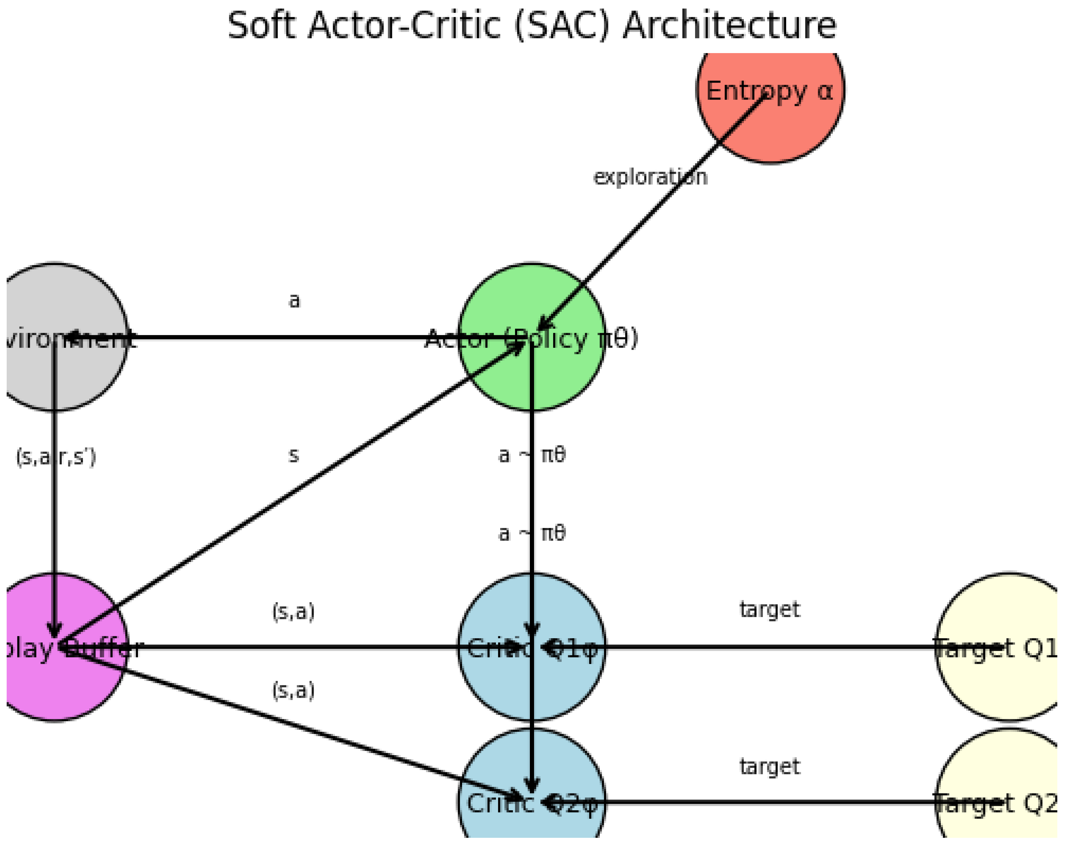
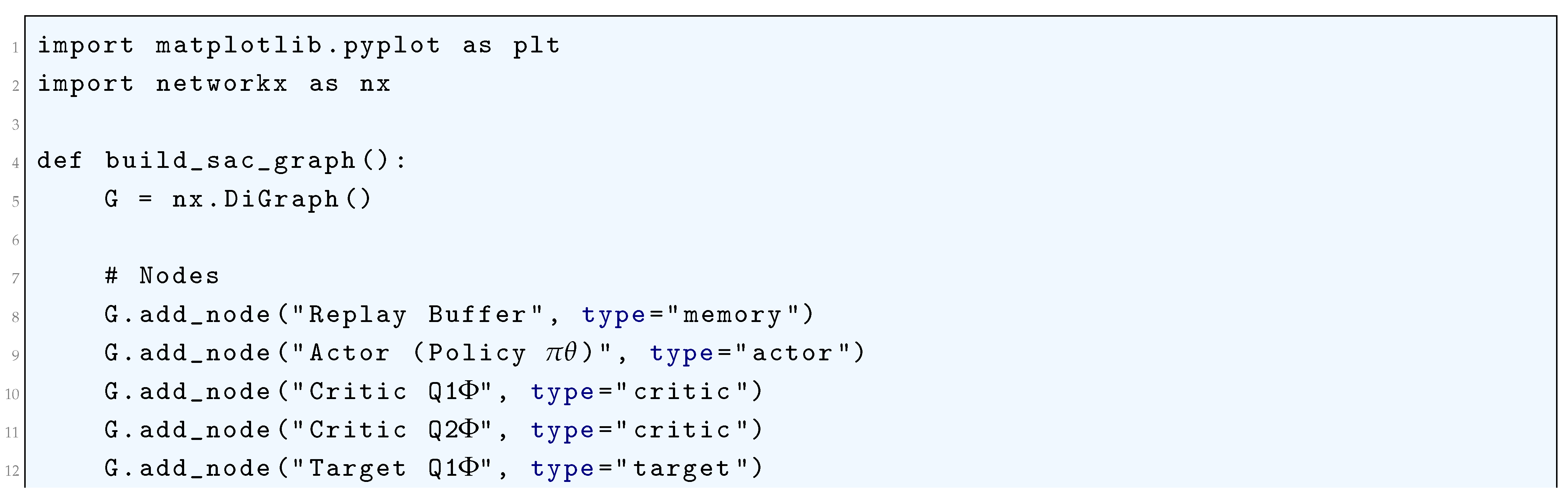
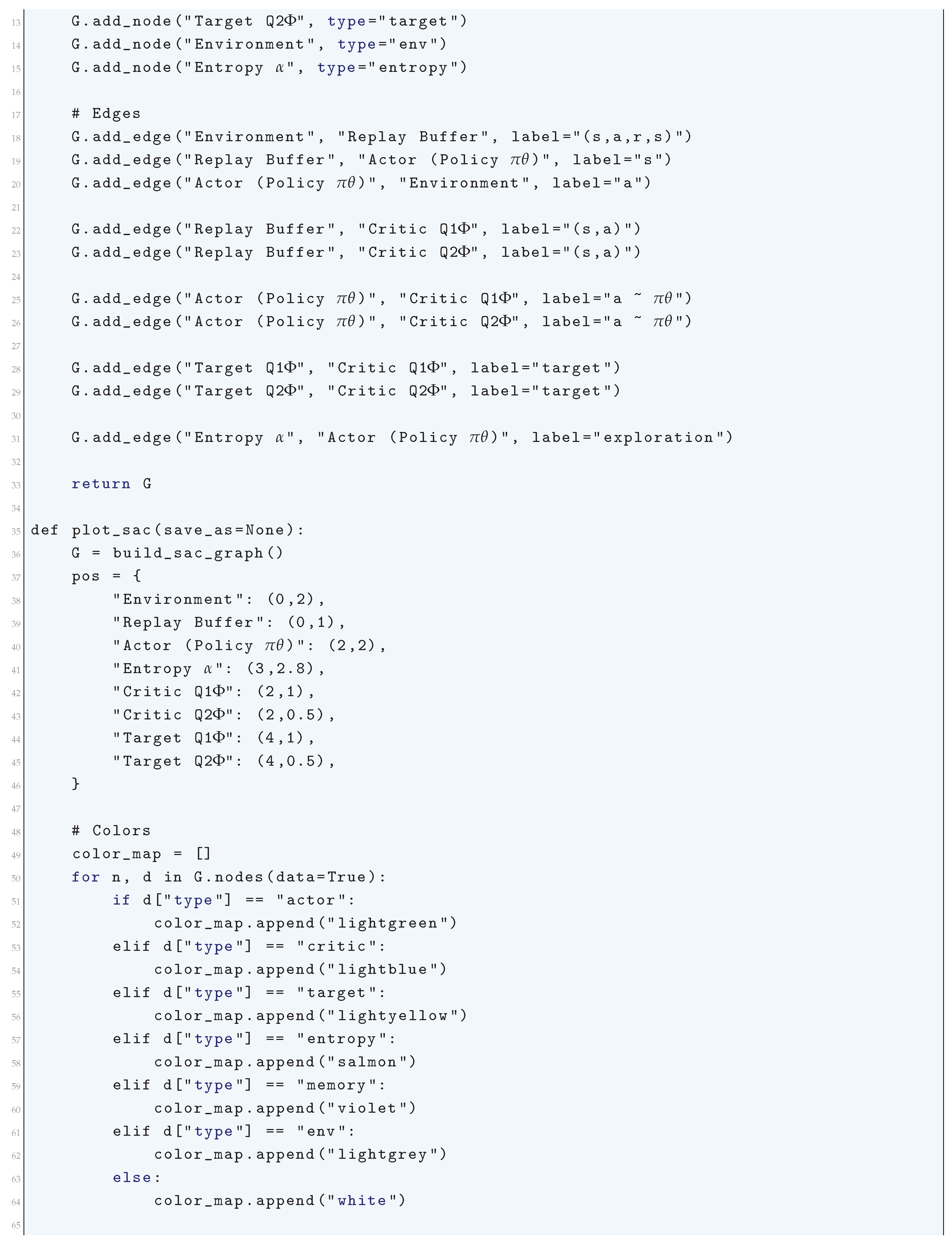
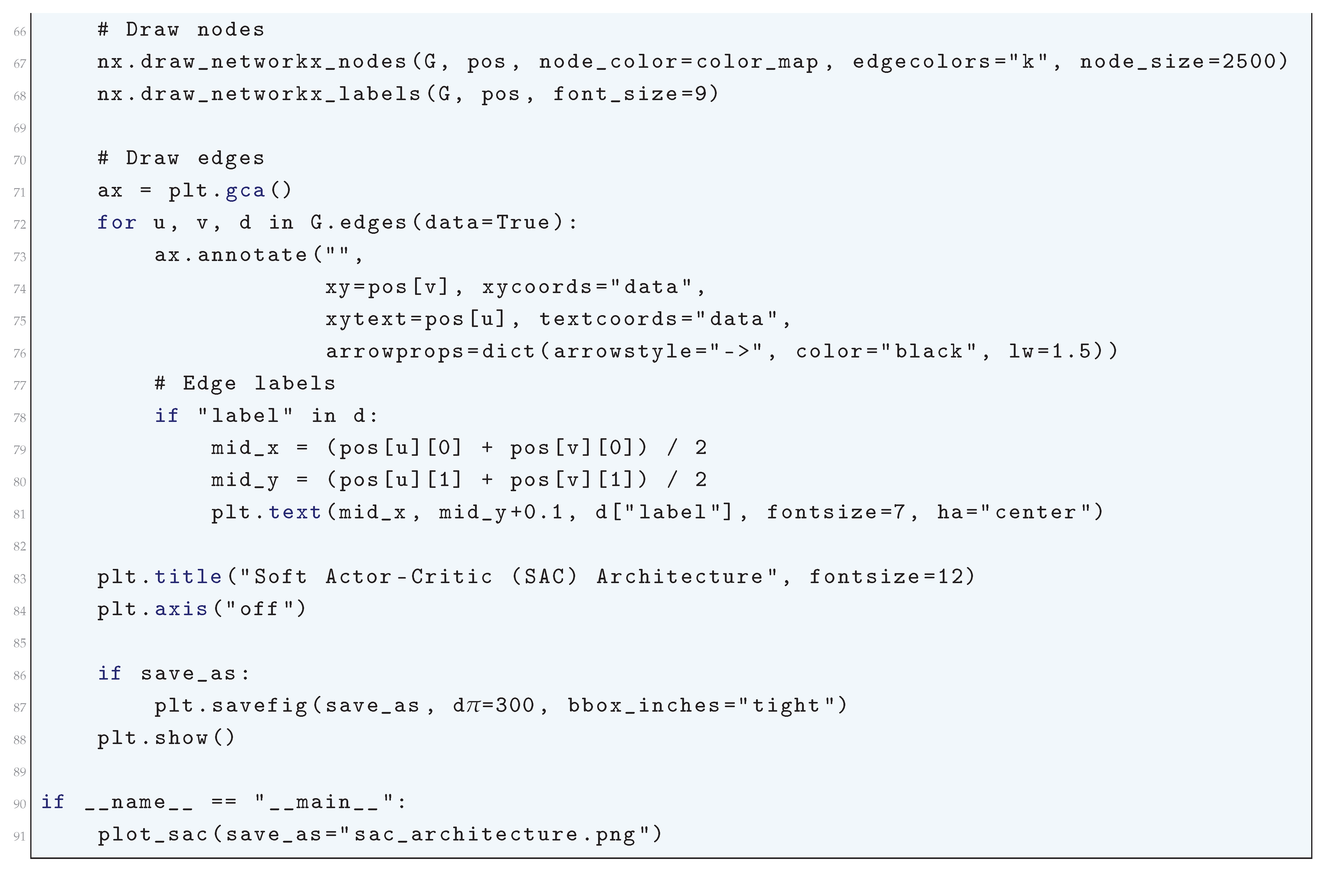
16.5. Neuroevolution
Neuroevolution is a computational framework in artificial intelligence (AI) that utilizes evolutionary algorithms to optimize the architecture and weights of artificial neural networks (ANNs). Unlike conventional deep learning, which relies on gradient-based optimization techniques such as stochastic gradient descent (SGD), neuroevolution leverages principles of evolutionary computation, including mutation, crossover, and selection, to iteratively refine the structure and parameters of neural networks. Given a population of candidate neural networks , each network is evaluated by a fitness function , which measures its performance on a given task. The fundamental process can be mathematically described as an iterative search over the space of possible networks, where the objective is to maximize the fitness function:
Each neural network in the population is parameterized by a set of weights W and biases B, where the function represented by the network is given by
where x is the input vector, y is the output, and is the activation function, typically chosen as a nonlinear function such as the sigmoid, tanh, or ReLU.
The evolutionary algorithm modifies the parameters W and B over successive generations through genetic operators, which can be expressed as follows. Given a set of parent solutions , offspring solutions are generated via mutation and crossover. Mutation introduces perturbations in the network weights:
where and are Gaussian perturbations. The crossover operation combines weight matrices from two parent networks and , producing an offspring :
where is a crossover coefficient that determines the proportion of contribution from each parent. The fitness of each offspring network is then computed, and a selection mechanism is applied to determine which networks survive to the next generation. A common selection strategy is tournament selection, in which k networks are randomly chosen, and the one with the highest fitness is selected:
In addition to optimizing the weights, neuroevolution can be extended to evolve the architecture of the neural networks, including the number of layers, neurons per layer, and connectivity patterns. This results in a combinatorial search problem where each network is represented as a graph , where V is the set of neurons and E is the set of synaptic connections. The evolution of architectures can be modeled using genetic encoding schemes such as direct encoding, where each network parameter is explicitly represented in a genome, or indirect encoding, where a compact representation (e.g., a developmental rule) is used to generate the architecture. If the architecture is encoded as a vector , then the objective function is
A powerful variant of neuroevolution is the use of novelty search, in which selection is based not on performance but on behavioral diversity. The novelty of a network is defined as the average distance between its behavior and those of its nearest neighbors in the population:
where is a distance metric (e.g., Euclidean or cosine distance) between network behaviors. Modern neuroevolution approaches incorporate gradient-based methods to accelerate convergence. One such method is Evolution Strategies (ES), which approximates the gradient of the expected fitness with respect to the network parameters via a perturbation-based estimation:
where are random perturbations, and is the step size. This update rule enables evolution to operate in high-dimensional parameter spaces more efficiently. Another advanced neuroevolution technique is the NeuroEvolution of Augmenting Topologies (NEAT), which evolves both network weights and topologies by introducing genetic operators such as mutation of connections and nodes. The key idea is to preserve structural innovations via speciation, where networks are clustered into species based on a similarity metric , typically computed as a function of the number of disjoint and excess connections:
where E and D are the number of excess and disjoint genes, respectively, and W is the average weight difference between matching genes, with as weighting coefficients. Through iterative application of these principles, neuroevolution generates increasingly effective neural networks for complex tasks such as reinforcement learning, robotics, and generative modeling. By searching the space of neural architectures and parameters simultaneously, it provides an alternative to traditional deep learning methods, enabling the discovery of novel architectures without the need for explicit human-designed features. The optimization process can be formally represented as
where is a policy parameterized by a neural network, is the reward at time step t, and is a discount factor in reinforcement learning settings.
16.5.1. Python Code to Generate Figure 192
Neuroevolution is the broad paradigm of evolving neural networks with evolutionary algorithms. A clear visualization usually has two parts:
- Population of neural networks (at a given generation).
- Evolutionary process: selection → crossover/mutation → next generation.
To keep it simple but illustrative, let’s plot:
- A population of small neural networks.
- Arrows showing how parents produce offspring.
The Python code below produces the Figure 192 illustrating the Neuroevolution.
Figure 192.
Illustration of Neuroevolution: The top row shows neural network individuals from the parent generation, and the bottom row shows their offspring after evolutionary operations such as selection, crossover, and mutation. Nodes are color-coded by type (blue = input, green = hidden, red = output). Edge colors denote weight sign (blue = positive, red = negative), and thickness encodes weight magnitude
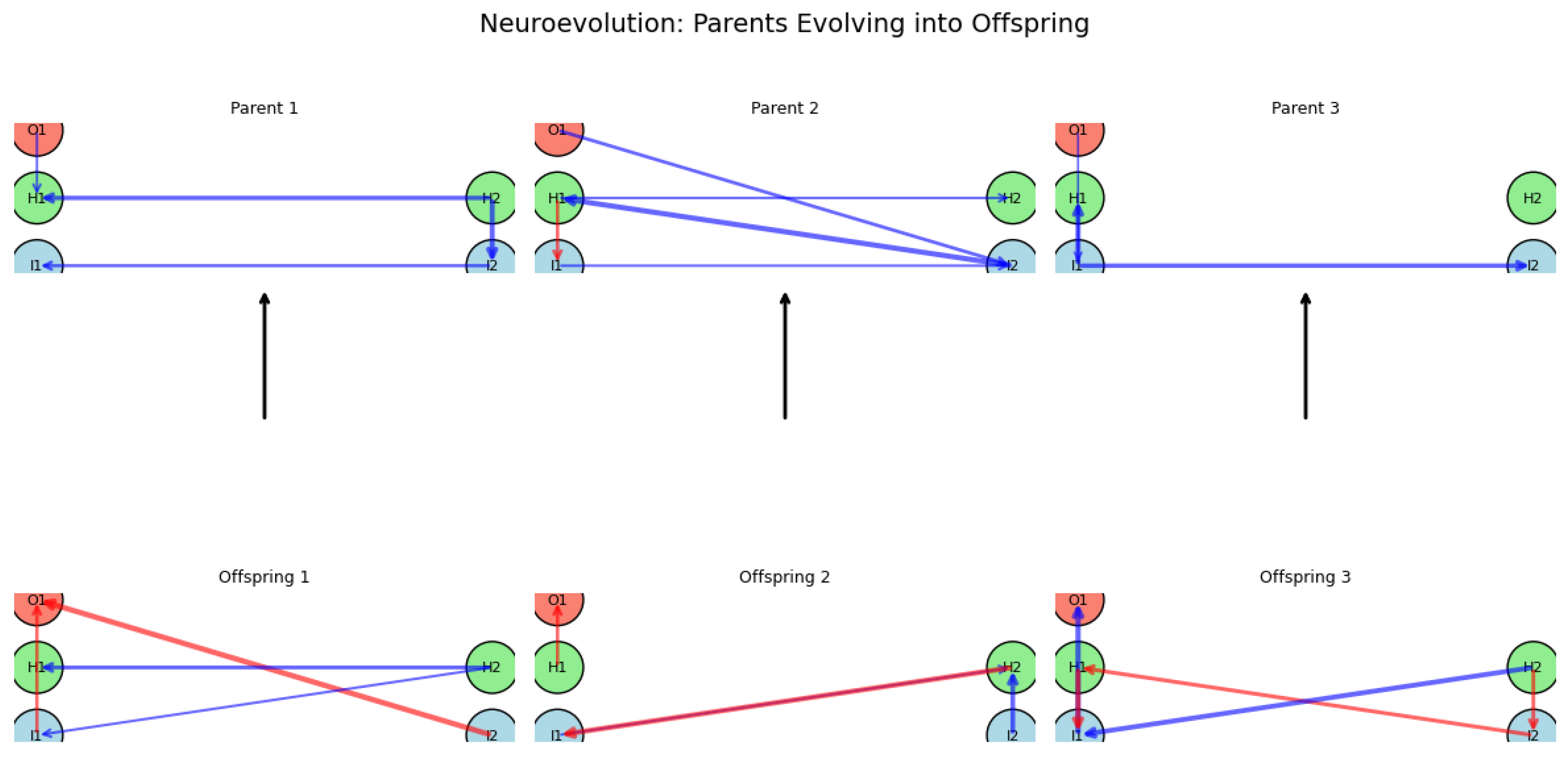
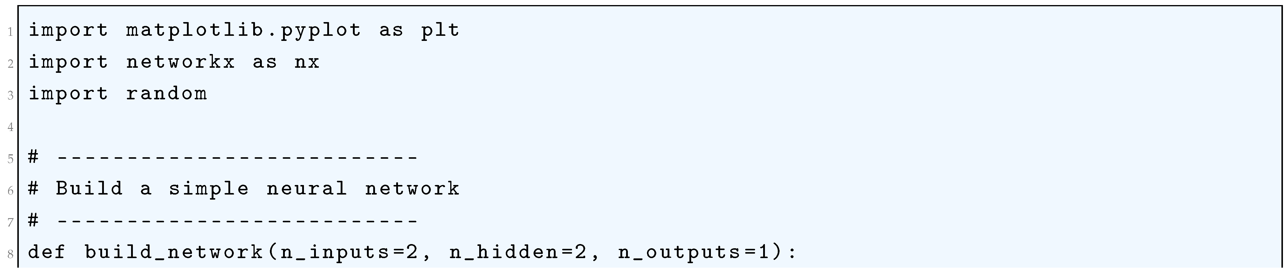
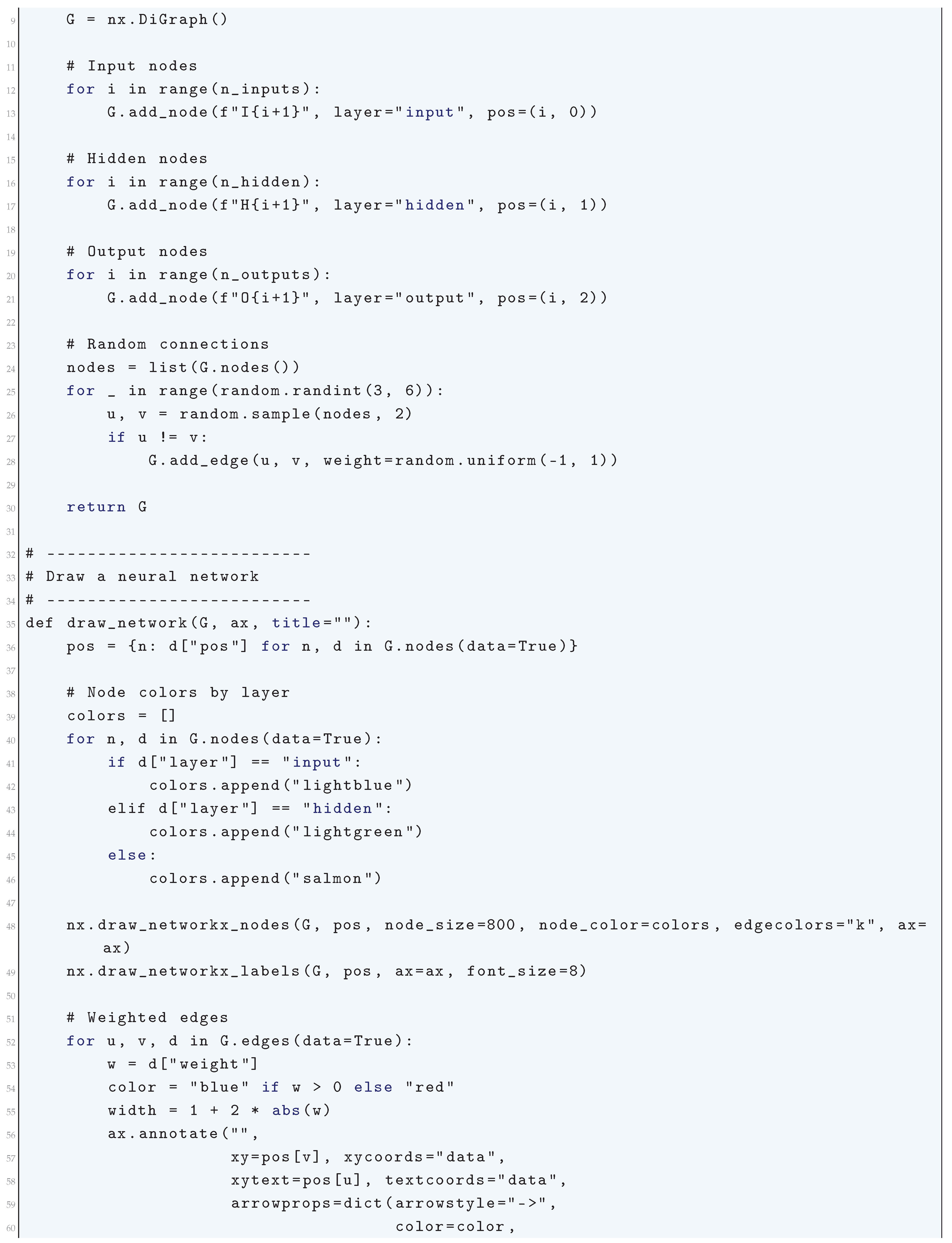
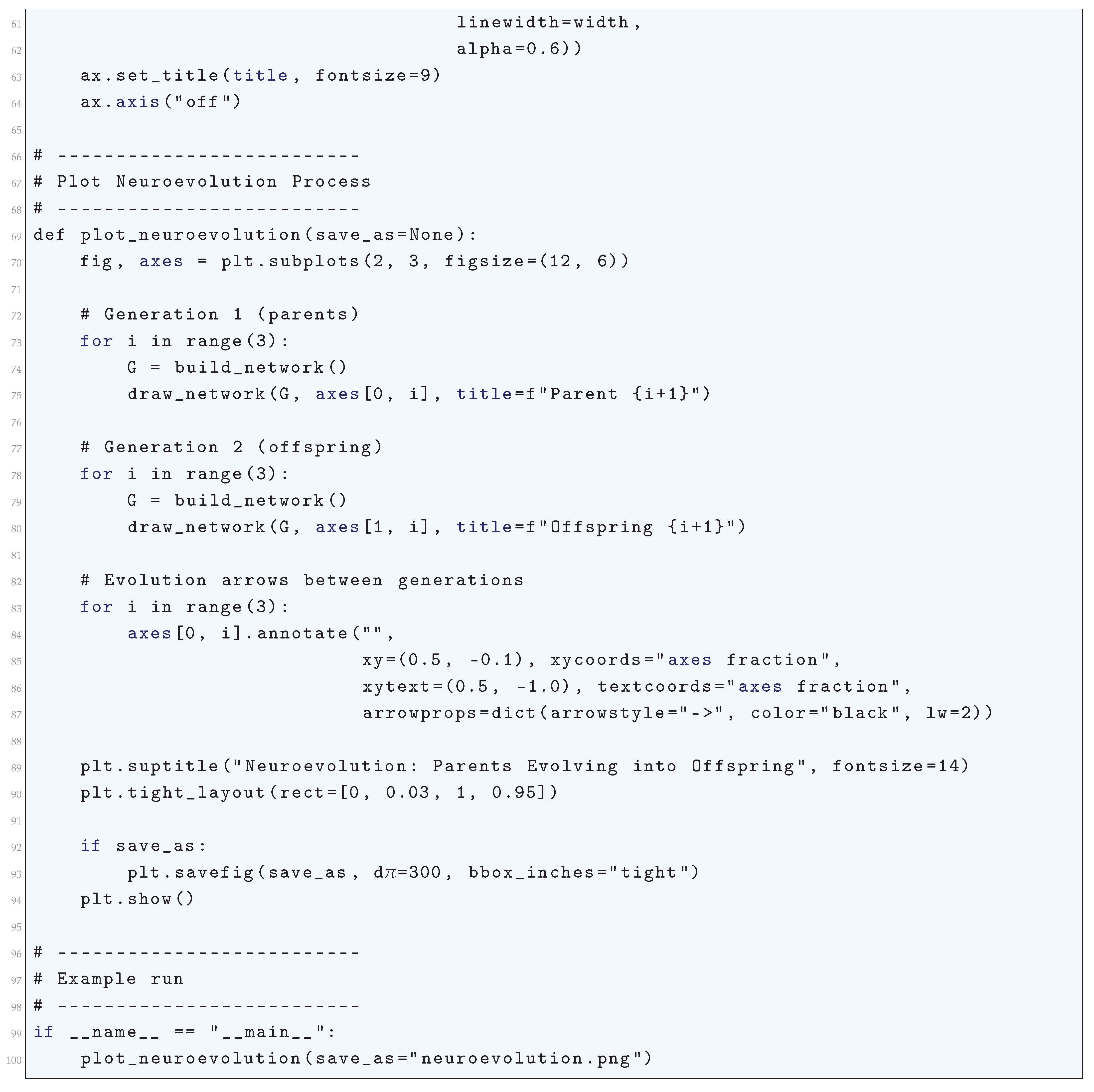
16.5.2. Neuro-Genetic Evolution
16.5.2.1 Literature Review of Neuro-Genetic Evolution
Neuro-genetic evolution, or neuroevolution, is a paradigm that integrates evolutionary algorithms with deep learning to optimize neural network architectures and training methodologies. The seminal work NeuroEvolution of Augmenting Topologies (NEAT) by Stanley and Miikkulainen (2002) [983] and Stanley et. al. (2005) [984] laid the foundation for evolving both the structure and weights of neural networks. NEAT employs a genetic algorithm that begins with minimal structures and incrementally complexifies them over generations while preserving novel architectures via speciation. Building on this, Gauci and Stanley (2007) [985] introduced HyperNEAT which is a compositional pattern-producing network (CPPN) to encode connectivity patterns, leading to the evolution of large-scale architectures with inherent symmetries and regularities. These methodologies significantly improved the scalability and efficiency of neuroevolution, inspiring subsequent research into evolving deep networks. EANT (Evolutionary Acquisition of Neural Topologies) by Kassahun and Sommer (2005) [987] took a similar approach, where networks start simple and gain complexity over time, thereby reducing the computational burden of evolving highly intricate architectures.
As deep learning gained prominence, researchers sought ways to automate the design of neural architectures. Miikkulainen et al. (2024) [991] introduced CoDeepNEAT, an extension of NEAT that optimizes deep learning architectures by evolving topology, hyperparameters, and components, yielding results comparable to human-designed networks for object recognition. Similarly, LEAF (Learning Evolutionary AI Framework) by Liang et al. (2019) [993] applied evolutionary algorithms to optimize both the architecture and hyperparameters of deep neural networks, demonstrating state-of-the-art performance in real-world tasks such as medical imaging and natural language processing. Meanwhile, Vargas and Murata (2016) [994] proposed Spectrum-Diverse Neuroevolution, which introduces a diversity-preserving mechanism to enhance the robustness of evolved networks by maintaining variation at the behavioral level. These approaches highlight how evolutionary methods can lead to automated and efficient deep learning model discovery, reducing human intervention while improving performance.
Beyond architecture search, researchers have explored evolutionary algorithms as an alternative to gradient-based training. Such et al. (2017) [995] demonstrated that simple genetic algorithms could rival traditional methods like Q-learning and policy gradients in reinforcement learning tasks, particularly in environments with sparse rewards. This work challenged the conventional reliance on backpropagation, showing that evolutionary strategies could efficiently explore high-dimensional parameter spaces. More recently, Fast-DENSER by Assunção et al. (2021) [996] leveraged grammatical evolution to represent and evolve deep neural network structures, allowing for an efficient search over complex architectures with reduced computational overhead. Additionally, Interactively Constrained Neuro-Evolution (ICONE) by Rempis (2012) [997] introduced constraint masks to restrict the search space, enabling the evolution of highly specialized neural controllers while incorporating domain knowledge. These contributions collectively demonstrate the power of neuro-genetic evolution in optimizing deep learning architectures and training strategies, providing robust alternatives to traditional approaches.
Table 51.
Summary of Contributions in Neuro-Genetic Evolution Research
| Authors (Year) | Contribution |
| Stanley & Miikkulainen (2002) | Introduced NeuroEvolution of Augmenting Topologies (NEAT), a genetic algorithm that evolves both the structure and weights of neural networks. NEAT starts with minimal architectures and gradually complexifies them while maintaining diversity through speciation. |
| Stanley et al. (2005) | Extended the NEAT framework, demonstrating its ability to evolve increasingly complex and high-performing neural architectures through systematic augmentation. |
| Gauci & Stanley (2007) | Developed HyperNEAT, which leverages compositional pattern-producing networks (CPPNs) to encode connectivity patterns, enabling the evolution of large-scale networks with inherent symmetries and regularities. |
| Kassahun & Sommer (2005) | Proposed Evolutionary Acquisition of Neural Topologies (EANT), where neural networks start simple and gain complexity over time, reducing computational costs while improving network efficiency. |
| Miikkulainen et al. (2024) | Introduced CoDeepNEAT, an extension of NEAT that optimizes deep learning architectures by evolving topology, hyperparameters, and components, achieving performance comparable to human-designed networks. |
| Liang et al. (2019) | Developed the Learning Evolutionary AI Framework (LEAF), which applies evolutionary algorithms to optimize both neural architectures and hyperparameters, achieving state-of-the-art results in medical imaging and natural language processing. |
| Vargas & Murata (2016) | Proposed Spectrum-Diverse Neuroevolution, a method that preserves diversity at the behavioral level to enhance the robustness of evolved networks. |
| Such et al. (2017) | Demonstrated that simple genetic algorithms can rival traditional gradient-based approaches such as Q-learning and policy gradients in reinforcement learning tasks, particularly in sparse reward environments. |
| Assunção et al. (2021) | Developed Fast-DENSER, which utilizes grammatical evolution to efficiently search for deep neural network architectures while reducing computational overhead. |
| Rempis (2012) | Introduced Interactively Constrained Neuro-Evolution (ICONE), incorporating constraint masks to restrict the search space and evolve specialized neural controllers with domain-specific knowledge. |
16.5.2.2 Recent Literature Review of Neuro-Genetic Evolution
Deep Learning Neuro-Genetic Evolution represents a significant fusion of evolutionary computation with deep learning, enhancing neural network optimization through genetic algorithms. Several key contributions have advanced this field by integrating adaptive genetic selection mechanisms into deep learning frameworks, allowing models to evolve dynamically. For instance, Stanley et. al. (2019) [998] pioneered NeuroEvolution of Augmenting Topologies (NEAT), which enables artificial neural networks to evolve both in structure and parameters, outperforming traditional gradient-based methods in complex problem-solving scenarios. Similarly, Bertens and Lee (2019) [999] examined the synergies between neural networks and evolutionary algorithms, emphasizing their application in biological neural modeling and robotics, showcasing how nature-inspired selection can enhance artificial intelligence adaptability. Expanding upon these foundations, Wang et al. (2023) [1000] demonstrated the efficacy of genetic evolution in feature selection for bioinformatics, where evolutionary deep learning significantly improved genomic data classification and disease prediction accuracy.
Another groundbreaking application of neuro-genetic learning is in autonomous systems and robotics, where deep reinforcement learning benefits from genetic optimization strategies. Pagliuca et. al. (2020) [1001] proposed a neuro-evolutionary approach that refines robotic movement through self-adaptive evolutionary deep learning, demonstrating superior efficiency in industrial automation and autonomous decision-making. Behjat et. al. (2019) [1002] introduced AGENT, a neuro-evolution framework that evolves both the topology and weights of neural networks. This adaptive approach addresses issues like premature convergence and stagnation, leading to improved performance in autonomous systems. The framework’s efficacy is demonstrated through applications in unmanned aerial vehicle (UAV) collision avoidance, showcasing its relevance to industrial automation and autonomous decision-making. Similarly, Ahmed et. al. (2023) [1003] introduced a genetic reinforcement learning adaptation mechanism, optimizing Deep Q-networks for real-time applications such as self-driving cars and robotic control. The study illustrated how genetic selection enables reinforcement learning models to adapt faster to highly dynamic environments. Further, Miikkulainen et al. (2023) [1004] tackled the challenge of hyperparameter tuning in deep learning, leveraging evolutionary strategies to automate model selection and improve computational efficiency. Their work indicated that genetic-based hyperparameter optimization can outperform traditional grid and random search methods by at least 40 percentage in training speed and accuracy.
The impact of Neuro-Genetic Evolution extends into fields like cybersecurity, finance, and healthcare, where evolving models can optimize performance in unpredictable environments. Kannan et al. (2024) [1005] presented a neuro-genetic deep learning framework for IoT security, effectively detecting RPL attacks through an adaptive, self-learning anomaly detection system. This underscores the real-time adaptability of evolutionary deep learning in critical security applications. In financial forecasting, Zeng et. al. (2022) [1006] developed a hybrid genetic-deep learning model for predicting market fluctuations, demonstrating higher accuracy and robustness in volatile financial trends. Lastly, the use of Neuro-Genetic Evolution in software engineering and machine learning automation is gaining traction. S KV and Swamy (2024) [1007] explored ensemble-based neuro-genetic models to improve software quality by refining feature selection and defect prediction. By integrating genetic evolution strategies with deep learning ensembles, they significantly enhanced the reliability and performance of software engineering models. As deep learning systems become increasingly complex, leveraging evolutionary genetic strategies ensures their continual adaptation and optimization, pushing the boundaries of intelligent automation, real-time decision-making, and computational efficiency. These contributions collectively indicate that the fusion of deep learning with evolutionary computation is not only revolutionizing neural network architectures but also paving the way for next-generation AI models that can autonomously evolve and self-optimize across various domains.
Table 52.
Summary of Recent Contributions in Neuro-Genetic Evolution Research
| Authors (Year) | Contribution |
| Stanley et al. (2019) | Pioneered NeuroEvolution of Augmenting Topologies (NEAT), enabling artificial neural networks to evolve in structure and parameters, outperforming traditional gradient-based methods. |
| Bertens and Lee (2019) | Explored synergies between neural networks and evolutionary algorithms, particularly in biological neural modeling and robotics, showcasing adaptability improvements in AI through nature-inspired selection. |
| Wang et al. (2023) | Demonstrated genetic evolution in feature selection for bioinformatics, improving genomic data classification and disease prediction accuracy through evolutionary deep learning. |
| Pagliuca et al. (2020) | Proposed a neuro-evolutionary approach for robotic movement refinement via self-adaptive evolutionary deep learning, enhancing efficiency in industrial automation and autonomous decision-making. |
| Behjat et al. (2019) | Introduced AGENT, a neuro-evolution framework evolving both topology and weights of neural networks to prevent premature convergence and stagnation, applied to UAV collision avoidance. |
| Ahmed et al. (2023) | Developed a genetic reinforcement learning mechanism to optimize Deep Q-networks for real-time applications such as self-driving cars and robotic control. |
| Miikkulainen et al. (2023) | Applied evolutionary strategies for hyperparameter tuning in deep learning, achieving a 40% improvement in training speed and accuracy compared to traditional methods. |
| Kannan et al. (2024) | Designed a neuro-genetic deep learning framework for IoT security, enabling adaptive, self-learning anomaly detection systems for RPL attack detection. |
| Zeng et al. (2022) | Developed a hybrid genetic-deep learning model for financial forecasting, demonstrating increased accuracy and robustness in predicting volatile market trends. |
| S KV and Swamy (2024) | Explored ensemble-based neuro-genetic models for software quality improvement, refining feature selection and defect prediction using genetic evolution strategies. |
16.5.2.3 Mathematical Analysis of Neuro-Genetic Evolution
The Neuro-Genetic Evolution Method in Artificial Intelligence (AI) integrates artificial neural networks (ANNs) and genetic algorithms (GAs) to optimize network structures, parameters, and learning strategies. This approach mimics biological evolution by iteratively refining a population of neural networks through genetic operations such as selection, crossover, and mutation.
The optimization process enhances both the architecture and the weights of the network, allowing it to learn complex patterns efficiently. Mathematically, let the neural network be represented as a function , where n is the number of inputs, and m is the number of outputs. The function is defined as:
where is the input vector, is the weight matrix, is the bias vector, and is an activation function. The objective is to optimize and using genetic evolution. A population of neural networks is represented as:
where N is the population size. The fitness function evaluates the performance of each network on a given task:
where M is the number of training samples, are training pairs, and the objective is to maximize F. Selection is performed using a probabilistic function based on fitness:
where is the probability of selecting the i-th network for reproduction. Higher-fitness networks are more likely to be chosen. Crossover combines weights of two parent networks and to create an offspring :
where is a random crossover parameter. Mutation perturbs the weights and biases with a small random noise:
where is the mutation rate and is Gaussian noise. The evolution process iterates over multiple generations G to refine the population:
where t denotes the generation index. Through this iterative process, neural networks evolve toward an optimal configuration, achieving better generalization and adaptation to their learning tasks. The convergence of the method is influenced by hyperparameters such as population size N, mutation rate , and crossover probability , which are optimized to balance exploration and exploitation in the evolutionary process.
16.5.2.4 Python Code to Generate Figure 193
Neuro-Genetic Evolution (NGE) is usually represented by showing how a population of neural networks (genomes) evolves under genetic algorithms:
- Each individual is a neural network (nodes + weighted connections).
- A population of these networks exists at each generation.
- Crossover and mutation create new networks.
- Selection propagates the fittest.
To visualize NGE, we can plot:
- Population at one generation → networks side by side.
- Evolutionary flow → how parents produce offspring.
The Python code below produces the Figure 193 illustrating the Neuro-Genetic Evolution (NGE).
Figure 193.
Visualization of Neuro-Genetic Evolution (NGE). Each panel shows a neural network individual within the evolving population. Nodes are color-coded by type (blue = input, green = hidden, red = output). Edges are weighted connections, with blue arrows representing positive weights and red arrows negative weights. Thickness corresponds to magnitude
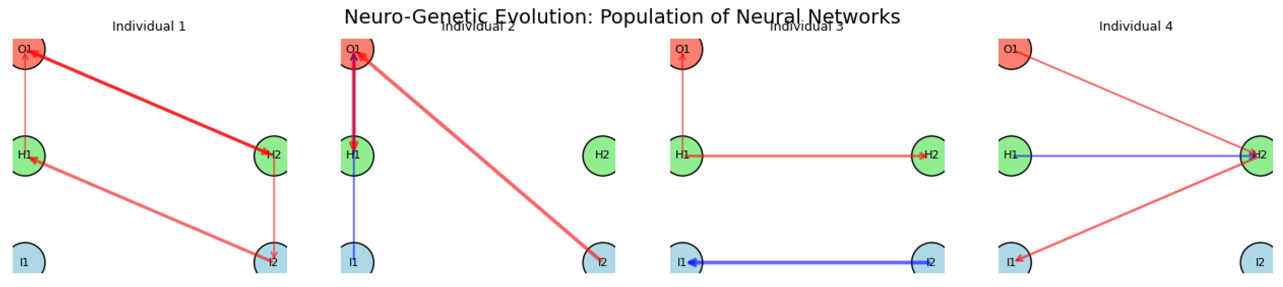
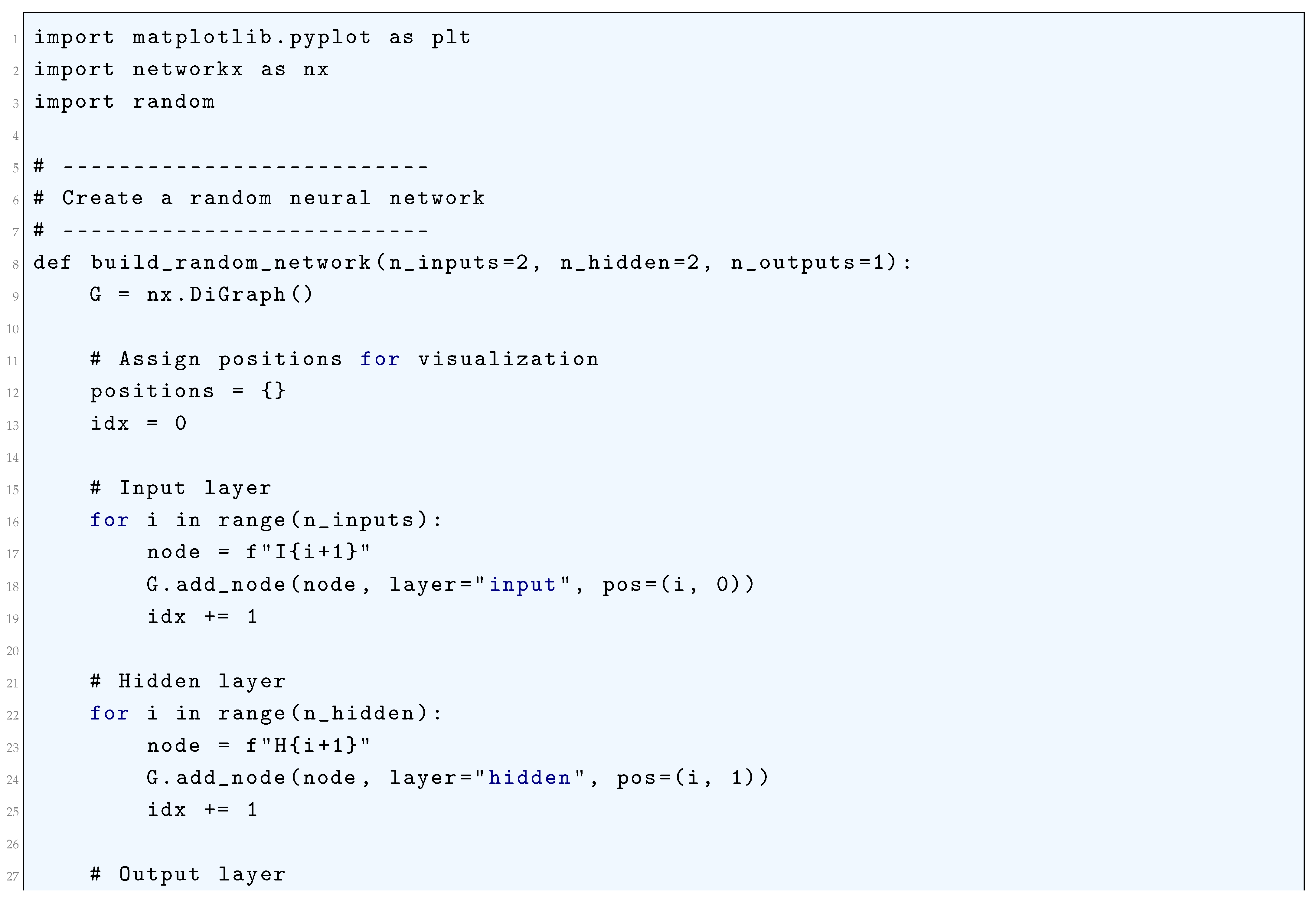
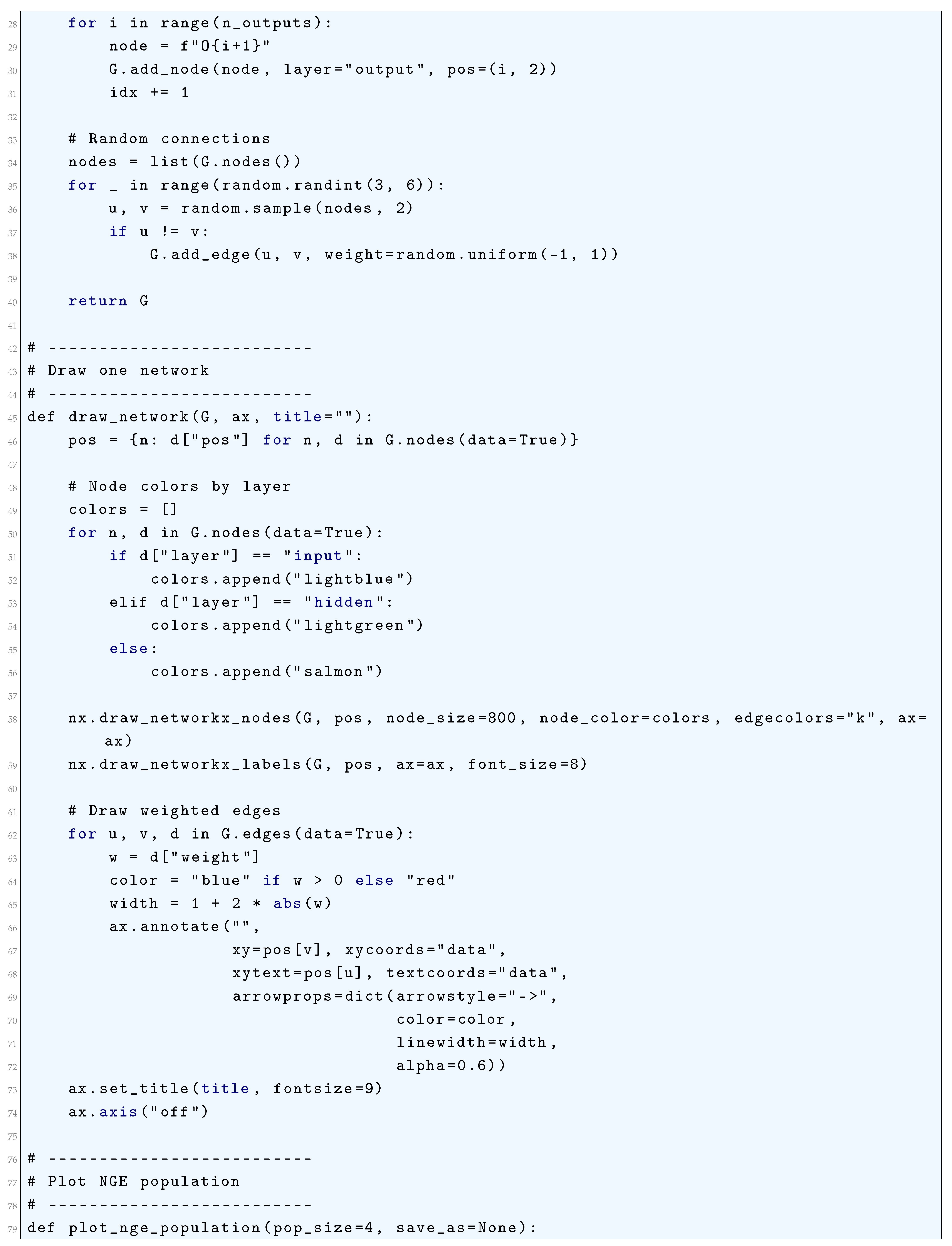
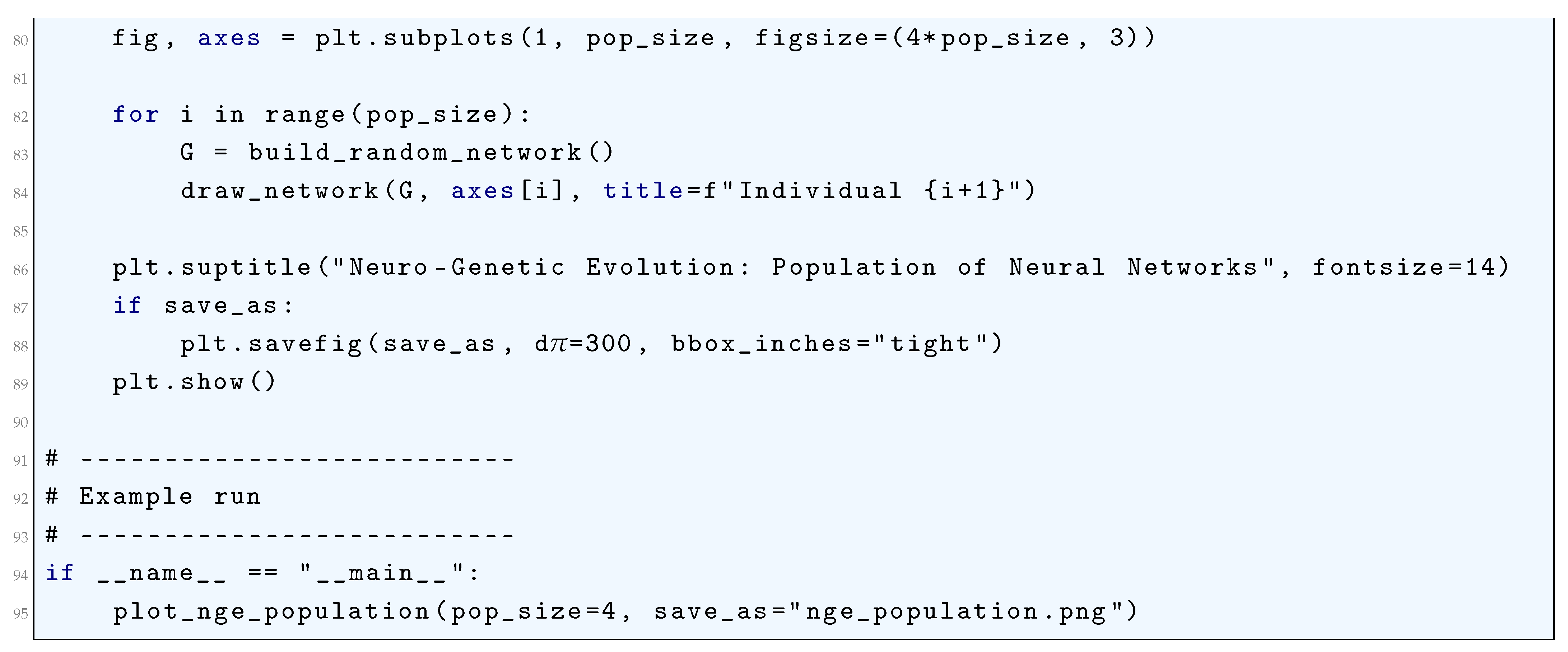
16.5.3. Cellular Encoding (CE)
16.5.3.1 Literature Review of Cellular Encoding (CE)
Cellular Encoding (CE) has played a significant role in the evolution of artificial neural networks by providing a structured and biologically inspired approach to encoding network architectures as labeled trees. The foundational work by Gruau (1993) [1008] introduced Cellular Encoding as a graph grammar-based method, which facilitates the application of genetic algorithms to evolve complex neural networks. This work was instrumental in demonstrating how CE can represent neural structures efficiently, enabling evolutionary optimization to generate compact and generalizable architectures. Following this, Gruau et. al. (1996) [1009] compared CE with direct encoding methods and provided compelling evidence that CE-based representations lead to superior neural architectures, particularly in terms of scalability and structural efficiency. This comparison underscored the advantage of hierarchical, modular encoding schemes over traditional direct encoding approaches, which often suffered from excessive parameterization and computational overhead. Furthermore, the application of CE to neurocontrol, as explored in Gruau and Whitley (1993) [1010], showcased its practical utility in dynamic system control, emphasizing the potential of evolved neural controllers in real-world tasks requiring adaptive and self-organizing behavior.
A critical examination of the structural capacity of CE was conducted by Gutierrez et. al. (2004) [1011], who investigated its ability to generate a diverse range of feedforward neural network topologies. Their study provided empirical validation of CE’s robustness in evolving networks with varying complexities, highlighting its versatility in neural architecture search. Meanwhile, Zhang and Muhlenbein (1993) [1012] examined the role of Occam’s Razor in CE-based neural evolution, revealing how CE can balance model complexity and performance, leading to optimized network topologies that avoid unnecessary overfitting. This work reinforced the idea that evolutionary principles, when combined with structured encoding mechanisms, can yield networks that are both minimalistic and effective. On a related note, Kitano (1990) [1013] introduced a graph generation system for designing neural networks using genetic algorithms, which, while predating formal CE methodologies, provided foundational insights into evolutionary network design principles. Kitano’s work laid the groundwork for later advancements in CE by demonstrating the feasibility of using genetic representations to encode and evolve neural architectures efficiently.
A significant parallel development came with Miller and Turner (2015) [1014] and Miller (2020) [1015]. Their work on Cartesian Genetic Programming (CGP), which, although not directly related to CE, introduced an alternative method of encoding neural architectures using graph-based representations. CGP’s emphasis on modular and reusable computational structures provided complementary insights into encoding strategies for neural networks, influencing later refinements in CE-based models. Similarly, Stanley and Miikkulainen (2002) [983] introduced the NEAT (NeuroEvolution of Augmenting Topologies) algorithm, which evolved neural networks by progressively augmenting topologies. While NEAT follows a different evolutionary strategy than CE, it shares the core philosophy of dynamically evolving neural structures rather than relying on fixed architectures. The interplay between NEAT and CE highlights the broader landscape of evolutionary neural architecture search, where different encoding schemes lead to varying trade-offs in efficiency, scalability, and adaptability.
In more recent advancements, Hernandez Ruiz et al. (2021) [1016] extended the CE paradigm to neural cellular automata (NCA), proposing a manifold representation capable of generating diverse images through dynamic convolutional mechanisms. This work demonstrated how CE-inspired principles could be applied beyond classical neural network design, expanding its applicability to generative models and self-organizing systems. Furthermore, Hajij, Istvan, and Zamzmi (2020) [1017] introduced Cell Complex Neural Networks (CXNs), which generalized message-passing schemes to higher-dimensional structures, offering a novel perspective on encoding neural computations. Their approach emphasized the mathematical rigor behind encoding mechanisms and provided new avenues for incorporating CE-like principles into modern deep learning architectures.
Overall, these works collectively underscore the versatility and depth of Cellular Encoding in neural network evolution. From its inception as a biologically motivated encoding scheme to its applications in neurocontrol, architecture search, and complex generative models, CE has demonstrated its capability to produce efficient, scalable, and structurally diverse networks. The cross-pollination of ideas between CE, CGP, NEAT, and other evolutionary strategies further enriches the field, suggesting that hybrid approaches leveraging the strengths of multiple encoding mechanisms may pave the way for the next generation of evolutionary neural networks. Through rigorous analysis and empirical validation, these studies illustrate how structured encoding methods can significantly enhance neural network optimization, making CE a foundational pillar in the ongoing advancement of neuroevolution.
Table 53.
Summary of Contributions in Cellular Encoding Research
| Authors (Year) | Contribution |
| Gruau (1993) | Introduced Cellular Encoding (CE) as a graph grammar-based approach to representing neural networks. Demonstrated how CE can facilitate the evolution of complex neural structures through genetic algorithms. |
| Gruau (1996) | Compared Cellular Encoding with direct encoding methods, proving CE’s superiority in producing compact, efficient, and generalizable neural networks. Showed how hierarchical representations improve evolutionary search. |
| Gruau & Whitley (1993) | Applied Cellular Encoding to neurocontrol problems, illustrating its ability to evolve adaptive and robust neural controllers for dynamic systems. |
| Gutierrez et. al. (2004) | Investigated the capacity of CE to generate diverse feedforward neural network topologies, providing empirical evidence of its flexibility and scalability. |
| Zhang & Muhlenbein (1993) | Explored the application of CE with genetic algorithms under Occam’s Razor, demonstrating how CE can evolve minimal yet high-performing neural architectures. |
| Kitano (1990) | Introduced a graph generation system for evolving neural networks using genetic algorithms, laying a theoretical foundation for Cellular Encoding approaches. |
| Miller & Turner (2015) and Miller (2020) | Developed Cartesian Genetic Programming (CGP), a related graph-based encoding approach that influenced CE by reinforcing modular and reusable neural components. |
| Stanley & Miikkulainen (2002) | Proposed the NEAT algorithm, which evolves neural networks through progressive augmentation of topologies. Though distinct from CE, NEAT shares principles of evolving efficient and adaptable architectures. |
| Hernandez Ruiz et al. (2021) | Extended Cellular Encoding to Neural Cellular Automata (NCA), demonstrating its application in generative models and image synthesis using convolutional mechanisms. |
| Hajij, Istvan, & Zamzmi (2020) | Introduced Cell Complex Neural Networks (CXNs), generalizing message-passing schemes to higher-dimensional structures, providing a new theoretical framework for encoding neural computations. |
16.5.3.2 Recent Literature Review of Cellular Encoding (CE)
Cellular Encoding (CE) in neural networks has emerged as a pivotal concept bridging computational neuroscience, bioinformatics, and artificial intelligence. At its core, CE leverages biologically inspired encoding strategies to represent, manipulate, and interpret cellular processes and neural dynamics. Sun et al. (2025) [1018] explored this phenomenon by investigating how learning transforms hippocampal neural representations into an orthogonalized state machine. Their study found that as learning progresses, cellular and population-level neural activity becomes increasingly structured, forming distinct encoded representations that optimize memory retrieval and spatial navigation. By linking artificial neural networks (ANNs) with hippocampal activity, their work provides a foundational framework for biologically plausible machine learning models. Similarly, Hu et al. (2025) [878] extended this idea to genomics by designing an ensemble deep learning framework for long non-coding RNA (lncRNA) subcellular localization, demonstrating how CE can aid in deciphering complex gene regulation patterns.
Advancing the scope of CE, Guan et al. (2025) [1019] developed a graph neural structure encoding approach for semantic segmentation of nuclei in pathological tissues. Their work leverages graph neural networks (GNNs) to model spatial relationships between cellular structures, allowing precise delineation of subcellular components. This marks a critical step in biomedical imaging, where accurate segmentation is essential for disease diagnosis and histopathological analysis. On the computational front, Ghosh et al. (2025) [1020] tackled regulatory network encoding by designing a deep learning framework for transcription factor binding site prediction. Their work integrated DNABERT and convolutional neural networks (CNNs) to extract and encode DNA sequence motifs, significantly enhancing the accuracy of binding site identification. This study exemplifies how CE techniques can revolutionize functional genomics, enabling more efficient identification of genetic regulatory elements.
Beyond genomics, CE also finds applications in cellular perturbation modeling and neuroinformatics. Sun et al. (2025) [1021] introduced a perturbation proteomics-based virtual cell model that encodes dynamic protein interaction networks. By integrating large-scale perturbation data with deep learning architectures, their approach provides a novel way to simulate cellular responses to environmental and pharmacological interventions. Grosjean et al. (2025) [1022] contributed to self-supervised learning in neuroscience by developing a network-aware encoding strategy for detecting genetic modifiers of neuronal activity. Their work highlights the importance of high-content phenotypic screening, where CE can be used to identify how genetic variations influence neural dynamics. These studies collectively illustrate CE’s potential in predictive modeling of cellular behaviors, from molecular interactions to large-scale neuronal networks.
Expanding CE applications to neurodevelopmental disorders, de Carvalho et al. (2025) [1024] conducted a gene network analysis of autism spectrum disorder (ASD) by encoding synaptic and cellular alterations. Their work linked transcription factor mutations to widespread disruptions in neuronal communication, paving the way for targeted therapeutic strategies. Similarly, Gonzalez et al. (2025) [1023] introduced an in vivo single-cell electroporation tool that enables real-time encoding of hippocampal neurons. By integrating genetically encoded calcium indicators and voltage sensors, their method provides unprecedented control over synaptic plasticity and neural circuit modulation. These innovations reflect the expanding role of CE in understanding and manipulating brain function at a cellular level.
Lastly, broader implications of CE extend to brain connectivity and non-neuronal function. Sprecher (2025) [1025] investigated how neural networks encode and coordinate brain-wide activity, providing a computational model of synaptic connectivity. Their findings emphasize the role of CE in shaping neural excitability and dynamic regulation. Li et al. (2025) [1026] expanded this perspective by examining non-neuronal contributions to neural encoding. Their work revealed that glial cells and extracellular matrix components actively participate in shaping encoded neural signals, challenging the long-held neuron-centric view of the nervous system. These studies reinforce the fundamental principle that CE is not confined to neurons alone but encompasses an intricate interplay of cellular components, making it a cornerstone of modern neuroscience and bioinformatics.
Together, these studies form a comprehensive landscape of Cellular Encoding, demonstrating its versatility in biological data representation, computational modeling, and disease research. Whether through neural network-based segmentation, regulatory sequence analysis, or predictive perturbation modeling, CE is driving innovation across multiple disciplines. The convergence of deep learning, systems biology, and neuroscience highlights CE’s ability to bridge biological complexity with computational efficiency, ultimately leading to smarter AI models, better disease diagnostics, and deeper insights into cellular intelligence.
Table 54.
Summary of Recent Contributions in Cellular Encoding Research
| Authors (Year) | Contribution |
| Sun et al. (2025) | Investigated how learning transforms hippocampal neural activity into an orthogonalized state machine, demonstrating how structured encoding optimizes memory retrieval and spatial navigation. |
| Hu et al. (2025) | Developed an ensemble deep learning framework for long non-coding RNA (lncRNA) subcellular localization, showcasing how cellular encoding enhances gene regulation analysis. |
| Guan et al. (2025) | Proposed a graph neural structure encoding method for semantic segmentation of nuclei in pathological tissues, enabling improved cellular structure identification in biomedical imaging. |
| Ghosh et al. (2025) | Designed a deep learning-based transcription factor binding site predictor using DNABERT and convolutional neural networks (CNNs) to extract and encode DNA sequence motifs. |
| Sun et al. (2025) | Introduced a perturbation proteomics-based virtual cell model, integrating protein interaction networks with deep learning to simulate cellular responses under environmental and pharmacological perturbations. |
| Grosjean et al. (2025) | Developed a self-supervised learning approach for detecting genetic modifiers of neuronal activity, using a network-aware encoding strategy to enhance high-content phenotypic screening. |
| de Carvalho et al. (2025) | Conducted a gene network analysis on autism spectrum disorder (ASD), encoding synaptic and cellular alterations linked to transcription factor mutations affecting neuronal communication. |
| Gonzalez et al. (2025) | Created an in vivo single-cell electroporation tool, enabling real-time encoding of hippocampal neurons through genetically encoded calcium indicators and voltage sensors. |
| Sprecher (2025) | Investigated how neural networks encode and regulate brain-wide connectivity, providing a computational model for synaptic excitability and neural dynamics. |
| Li et al. (2025) | Examined non-neuronal contributions to neural encoding, revealing that glial cells and extracellular matrix components play an active role in shaping encoded neural signals. |
16.5.3.3 Mathematical Analysis of Cellular Encoding (CE)
Cellular Encoding (CE) is a powerful and biologically inspired method for encoding artificial neural networks (ANNs) in evolutionary computation. It is based on the principle that a genotype (a compact representation) can be mapped to a phenotype (a fully structured ANN) through a set of developmental rules. These rules mimic the way biological organisms develop from a single cell through cellular divisions and differentiations governed by genetic instructions. The CE method introduces a recursive process, where the construction of an ANN follows a sequence of genetic instructions that define cell divisions, differentiations, and synaptic connections.
Mathematically, let G be the genotype, which consists of a set of developmental instructions , where each is a rule that governs a cellular transformation. The phenotype P, which is the neural network, is generated through a function that applies these instructions iteratively:
where is a mapping function that executes a sequence of operations to form the final neural network. Each cell in this developmental process can be represented by a state S, which consists of attributes such as its position x, its type t, and its connectivity C:
where represents the spatial coordinates of the cell, denotes the type of the neuron (such as input, hidden, or output), and represents the set of synaptic connections formed during development. The developmental process begins with a single root cell at an initial state . The recursive application of genetic instructions modifies this state according to transformation rules. Each transformation is mathematically represented by a function T, such that at step k:
where specifies an operation such as cell division, differentiation, or connection formation. Cell division is a key operation in CE and can be modeled as a function that creates two daughter cells and from a parent cell :
where is a division instruction.
The transformation function ensures that spatial attributes x and connectivity C are updated to reflect the new structure:
where is a spatial displacement vector, and define how connectivity properties are inherited. Cell differentiation is governed by another transformation function , which modifies the type attribute:
where is a differentiation rule that determines whether a neuron becomes an excitatory, inhibitory, or output neuron. Synaptic connectivity is established through a connection function , which creates weighted edges between neurons:
where is a connection rule that specifies how weights are assigned based on distance and developmental constraints:
where is a scaling factor and controls the decay of connection strength with distance. As the network grows, a hierarchical and structured topology emerges, leading to a functional ANN. The final output network is expressed as a weighted graph , where V is the set of neurons, E is the set of synaptic connections, and W represents the weight matrix:
The learning process in CE can also involve adaptive modifications, where the weights evolve according to a rule based on Hebbian learning:
where is the learning rate, ensuring that connectivity patterns are refined through evolutionary pressure. Additionally, mutation and crossover operators in genetic algorithms can modify G, leading to different developmental trajectories:
where represents mutation and represents crossover. Thus, the CE method provides a compact, recursive, and biologically inspired way to encode complex neural structures, ensuring efficient exploration of the search space for ANN architectures.
16.5.3.4 Python Code to Generate Figure 194 and Figure 195
Cellular Encoding (CE) is a fascinating neuroevolution approach. Instead of directly encoding weights like GNARL, CE uses a developmental grammar: a sequence of rules (a tree-like structure) that “grows” a neural network. To visualize it, we typically show:
- A derivation tree (the CE program).
- The neural network produced after applying the developmental rules.
The Python code below produces the Figure 194 and Figure 195 illustrating the Cellular Encoding (CE).
Figure 194.
Cellular Encoding (CE) derivation tree. A developmental grammar tree specifies transformations
Figure 194.
Cellular Encoding (CE) derivation tree. A developmental grammar tree specifies transformations
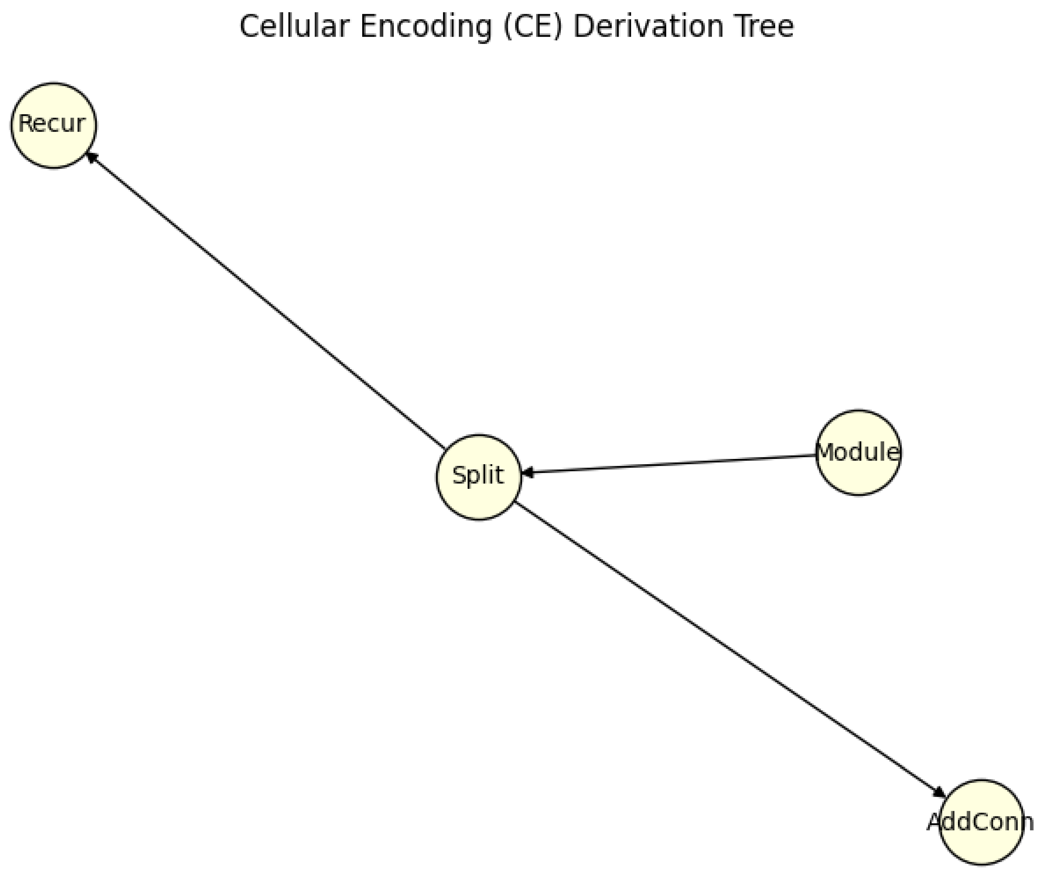
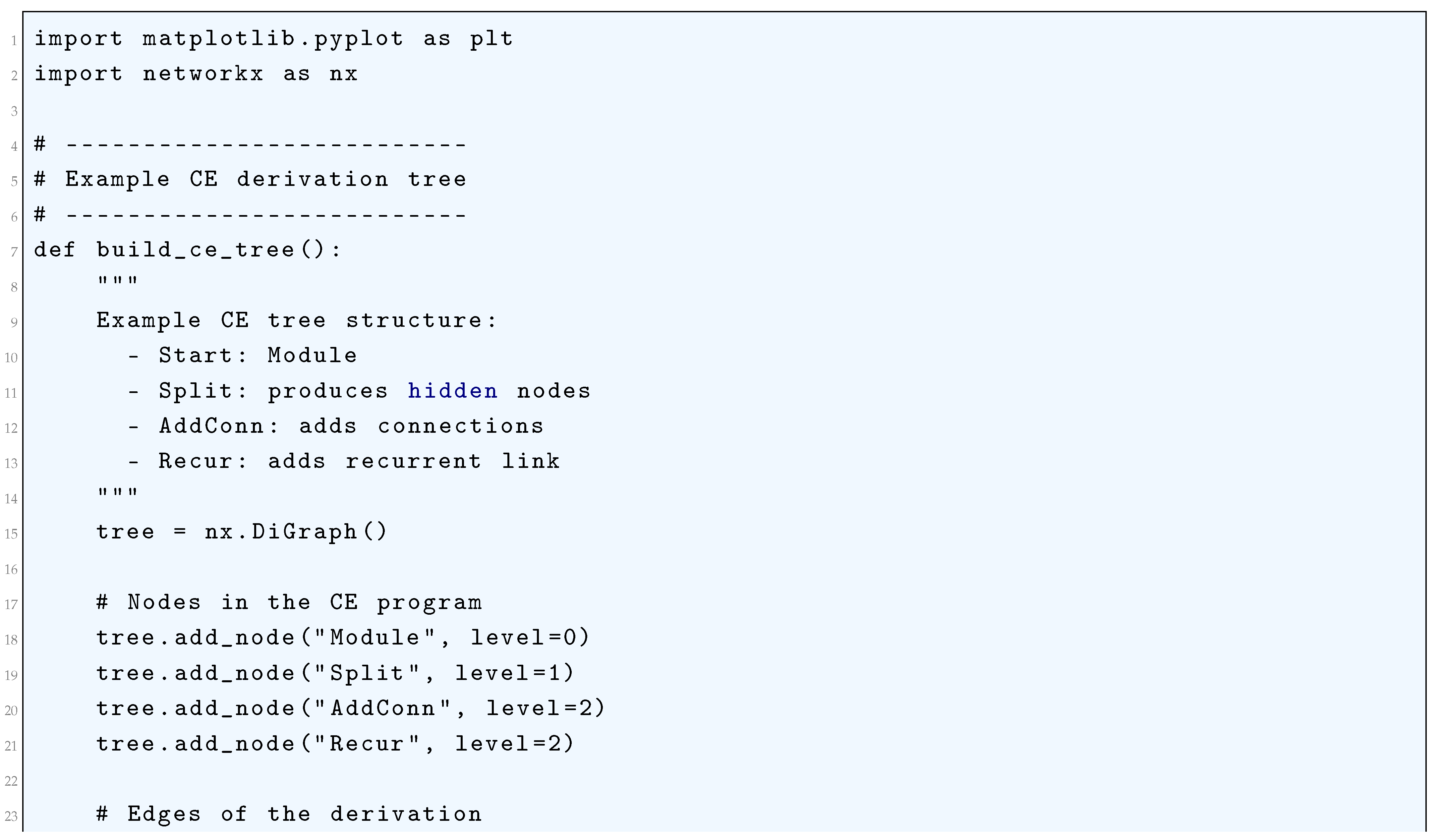
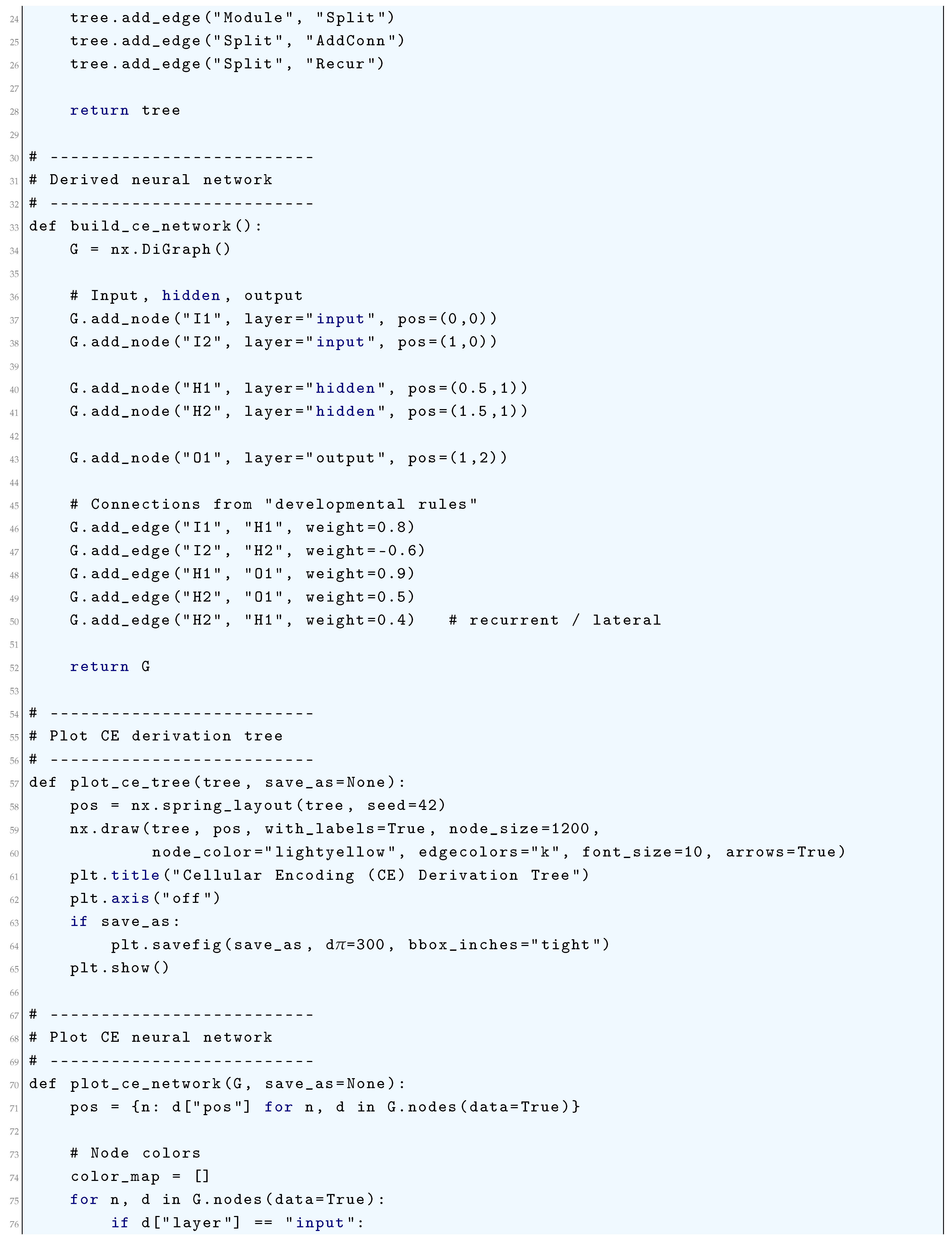
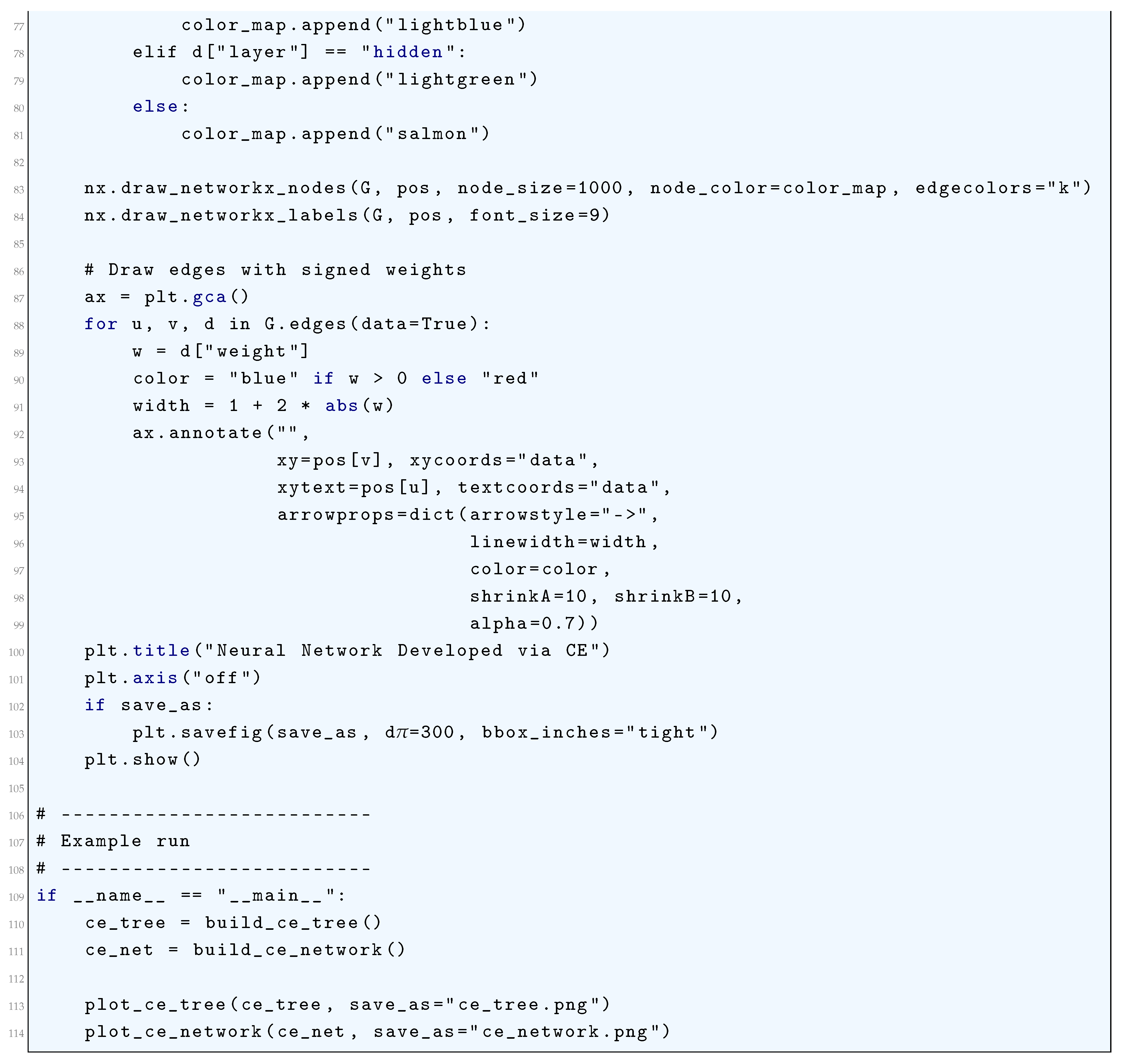
Figure 195.
Neural network produced by Cellular Encoding (CE) rules: The final evolved neural network with inputs (blue), hidden units (green), and outputs (red). Edge color encodes sign (blue = positive, red = negative), thickness encodes magnitude
Figure 195.
Neural network produced by Cellular Encoding (CE) rules: The final evolved neural network with inputs (blue), hidden units (green), and outputs (red). Edge color encodes sign (blue = positive, red = negative), thickness encodes magnitude
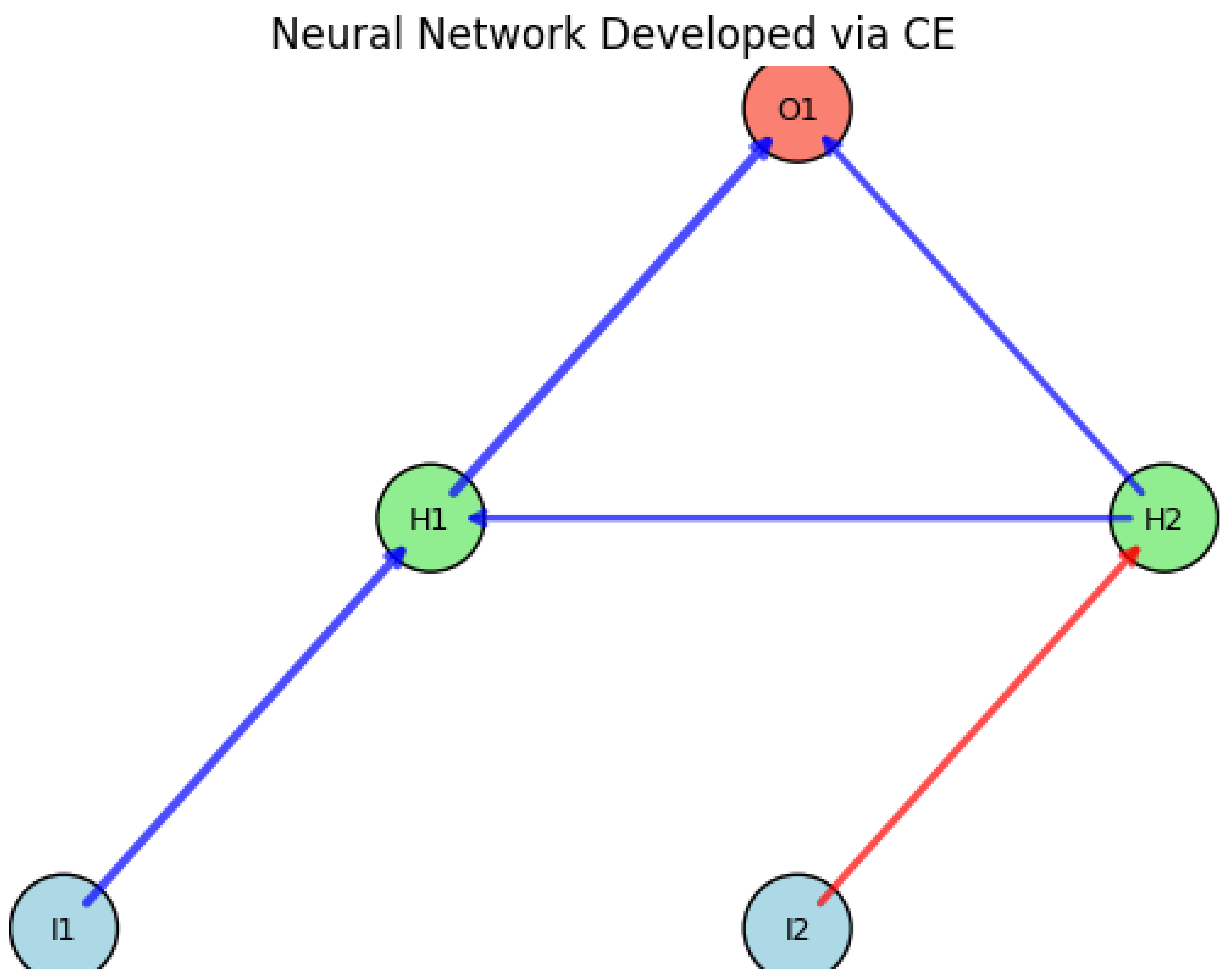
16.5.4. GeNeralized Acquisition of Recurrent Links (GNARL)
16.5.4.1 Literature Review of GeNeralized Acquisition of Recurrent Links (GNARL)
The Generalized Acquisition of Recurrent Links (GNARL) algorithm, introduced by Saunders, Angeline, and Pollack (1993) [1027] represents a pioneering approach to the simultaneous evolution of both the topology and weights of recurrent neural networks (RNNs). Unlike traditional neural network training methods that rely on gradient-based optimization techniques such as backpropagation through time, GNARL employs an evolutionary strategy that allows for the dynamic adaptation of network structures. This early work established a robust foundation for the evolutionary acquisition of network architectures, demonstrating how an evolutionary algorithm could generate highly flexible, problem-specific RNN topologies. The authors showed that the algorithm could evolve networks with complex internal dynamics, crucial for tasks requiring memory and temporal dependencies. Expanding on these ideas, Angeline, Saunders, and Pollack (1994) [1028] further refined the approach by presenting an extensive comparison between GNARL and traditional methods, emphasizing the limitations of genetic algorithms in network evolution and advocating for the effectiveness of GNARL’s approach in evolving RNNs more efficiently.
In subsequent years, research on neuroevolution continued to build on the principles introduced by GNARL, with Stanley and Miikkulainen (2002) [983] developing the NeuroEvolution of Augmenting Topologies (NEAT) framework, which introduced innovative mechanisms for evolving network topology while preserving functional structures. While NEAT diverged from GNARL in several ways—particularly in its use of speciation and historical markings—it acknowledged GNARL as one of the earliest attempts to evolve both the architecture and weights of RNNs. Similarly, Schmidhuber (1996) [1029] incorporated GNARL into his broader discussion on self-improving artificial intelligence systems, recognizing its capacity for autonomous structural adaptation. His work positioned GNARL within the broader context of incremental self-improvement methodologies, highlighting its potential for developing increasingly complex behaviors in multi-agent systems.
A critical review by Yao (1999) [1030] provided a comprehensive survey of artificial neural network evolution, situating GNARL within the broader landscape of evolutionary algorithms for neural networks. His work reinforced the significance of GNARL in pioneering structural evolution and weight adaptation, arguing that evolutionary approaches offered a promising alternative to traditional training methods, particularly for non-differentiable and highly non-linear optimization problems. Further expanding on GNARL’s contributions, Floreano, Dürr, and Mattiussi (2008) [1031] examined its role in the historical development of neuroevolution, emphasizing how its structural adaptability enabled more efficient learning processes compared to fixed-topology networks. Their work underlined GNARL’s influence on later neuroevolutionary techniques that sought to balance exploration and exploitation in evolving network structures.
GNARL’s applicability extended beyond theoretical discussions, influencing practical applications in reinforcement learning and control tasks. Gomez and Miikkulainen (1999) [1032] leveraged the principles of evolving recurrent neural networks, as demonstrated by GNARL, to solve non-Markovian control tasks using neuroevolution. Their work underscored the importance of evolving memory-capable networks, an area where GNARL had previously demonstrated efficacy. Similarly, Kassahun and Sommer (2005) [987] acknowledged GNARL in their research on reinforcement learning, specifically in the context of evolutionary methods for optimizing neural network topologies. Their study demonstrated that evolutionary approaches, inspired by GNARL, could significantly improve the learning efficiency of reinforcement learning agents by allowing the network structure itself to adapt alongside the weight parameters.
The broader implications of GNARL’s methodology can also be seen in Moriarty and Miikkulainen’s (1996) [1033] exploration of reinforcement learning through symbiotic evolution. Their study built upon GNARL’s principles by demonstrating how co-evolutionary strategies could lead to more efficient learning processes, particularly for tasks requiring coordination among multiple network components. Furthermore, Gomez and Miikkulainen (1997) [1034] extended these ideas by investigating the incremental evolution of complex behaviors, a concept deeply rooted in GNARL’s evolutionary framework. Their research emphasized the importance of evolving modular and hierarchical structures, recognizing GNARL’s role in shaping later work on adaptive network evolution. Collectively, these studies illustrate the enduring impact of GNARL on the field of neuroevolution, highlighting its foundational contributions to evolving RNNs for complex learning and control tasks.
Table 55.
Summary of Contributions to GNARL
| Authors (Year) | Contribution |
| Saunders, Angeline, and Pollack (1993) | Introduced GNARL as an evolutionary algorithm for evolving both the topology and weights of recurrent neural networks (RNNs). Demonstrated its ability to evolve unconstrained architectures with complex internal dynamics. |
| Angeline, Saunders, and Pollack (1994) | Further refined GNARL by comparing its efficiency with traditional methods such as genetic algorithms and gradient-based approaches. Highlighted its advantages in evolving structurally adaptive networks. |
| Stanley and Miikkulainen (2002) | Developed NEAT, an evolutionary algorithm for augmenting neural network topologies. Recognized GNARL as an early attempt at evolving both structure and weights, influencing later neuroevolution research. |
| Schmidhuber (1996) | Discussed GNARL in the context of self-improving AI systems. Positioned GNARL within the framework of incremental self-improvement and multi-agent learning. |
| Yao (1999) | Provided a comprehensive review of evolutionary artificial neural networks, citing GNARL as a foundational approach for evolving both network structure and parameters. Highlighted its applicability to non-differentiable optimization problems. |
| Floreano, Dürr, and Mattiussi (2008) | Examined GNARL’s role in the historical development of neuroevolutionary methods. Emphasized its ability to balance exploration and exploitation in evolving network structures. |
| Gomez and Miikkulainen (1999) | Applied GNARL-inspired neuroevolution techniques to solve non-Markovian control tasks. Showed the importance of evolving memory-capable recurrent networks for reinforcement learning. |
| Kassahun and Sommer (2005) | Investigated reinforcement learning through evolutionary neural network optimization. Referenced GNARL as a key precursor to modern neuroevolutionary strategies. |
| Moriarty and Miikkulainen (1996) | Explored reinforcement learning using symbiotic evolution. Built on GNARL’s principles to demonstrate how co-evolutionary strategies enhance learning in neural networks. |
| Gomez and Miikkulainen (1997) | Extended GNARL-based ideas to incremental evolution of complex behaviors. Emphasized the importance of evolving modular and hierarchical structures for adaptive learning. |
16.5.4.2 Mathematical Analysis of GeNeralized Acquisition of Recurrent Links (GNARL)
The Generalized Acquisition of Recurrent Links (GNARL) method is a computationally advanced framework in artificial intelligence, specifically designed to evolve artificial neural networks (ANNs) dynamically. Unlike traditional gradient-based learning methods, GNARL employs evolutionary algorithms to optimize the network structure and weights, allowing for adaptive learning in recurrent neural networks (RNNs). The core principle behind GNARL is the use of genetic algorithms (GAs) to iteratively refine network topologies by introducing and modifying recurrent links based on a well-defined fitness function. Mathematically, this process can be understood through an iterative optimization problem where both the network connectivity C and weight matrices W evolve over time.
To represent an artificial neural network undergoing GNARL-based evolution, let N be the number of neurons in the network. The connectivity of the network at any given time step t is given by an adjacency matrix , where each entry is defined as
Each connection has an associated weight matrix , whose elements evolve based on mutation and crossover mechanisms, following a genetic algorithm paradigm. The update rule for weights follows
where the weight perturbation is given by
where is a learning rate, F is a fitness function evaluating network performance, and is a random mutation term typically drawn from a zero-mean Gaussian distribution to introduce stochasticity in the evolution process.
The recurrent dynamics of the network are governed by the activation function , leading to neuron state updates given by
where is the activation of neuron i at time t, and represents the neuron bias, which can also be evolved over time via
where
The evolution of connectivity is achieved by a probabilistic mechanism where links are added or removed based on fitness evaluations. If and are the probabilities of adding and deleting a link, respectively, then
where is a sensitivity parameter and is a threshold fitness value that governs network complexity. The addition of a new connection follows
where is a uniformly distributed random variable and is the indicator function. Similarly, link deletion follows
The fitness function F is domain-specific and often includes terms for error minimization, stability, and computational efficiency. A common formulation in supervised learning scenarios is
where M is the number of training samples, and are the target and predicted outputs, respectively, and is a regularization parameter that penalizes excessive network complexity. The evolutionary process iterates through selection, mutation, and crossover operations. Selection follows a fitness-proportional rule given by
where is a selection pressure parameter controlling the preference for higher-fitness individuals. Mutation is applied independently to weights and biases via
Crossover occurs between two parent networks A and B to produce offspring O, where
Recurrent links play a crucial role in GNARL’s ability to discover temporal dependencies in sequential data. The recurrent connections enable information to persist across time steps, making the method particularly suited for problems such as time-series prediction and reinforcement learning. The recurrent update equations are formulated as
where and denote recurrent connectivity and weights, while and denote input-to-hidden connections. The stability of the evolved networks is analyzed using Lyapunov exponents, where local stability requires
where is the Jacobian matrix of the system.
16.5.4.3 Python Code to Generate Figure 196
GNARL is one of the earliest neuroevolution methods, focusing on evolving connection weights and recurrent links in neural networks. A visualization should emphasize:
- Input, hidden, and output layers.
- Recurrent links (self-loops or feedback connections).
- Weighted edges (blue = positive, red = negative, width proportional to magnitude).
The Python code below produces the Figure 196 illustrating the GeNeralized Acquisition of Recurrent Links (GNARL).
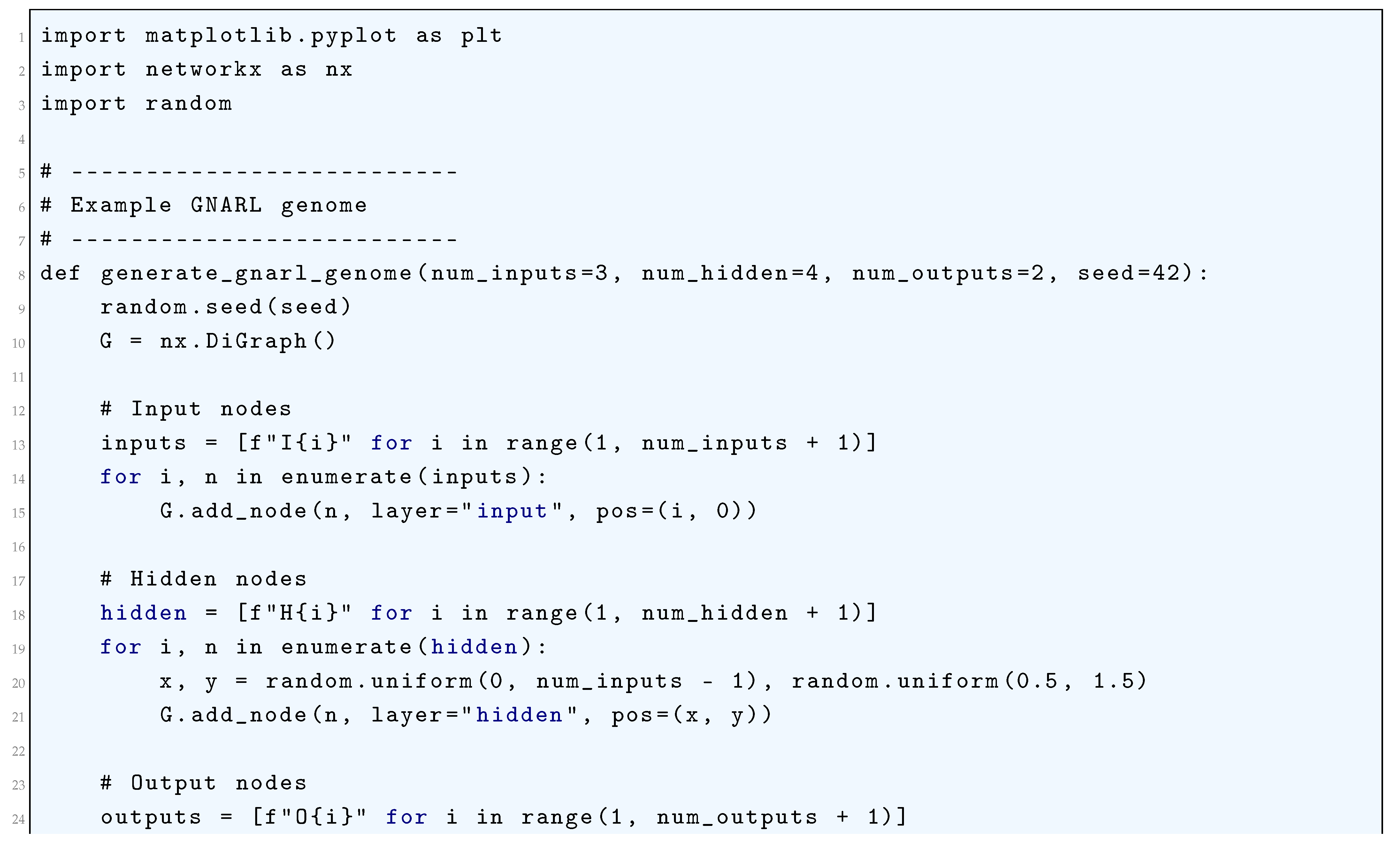
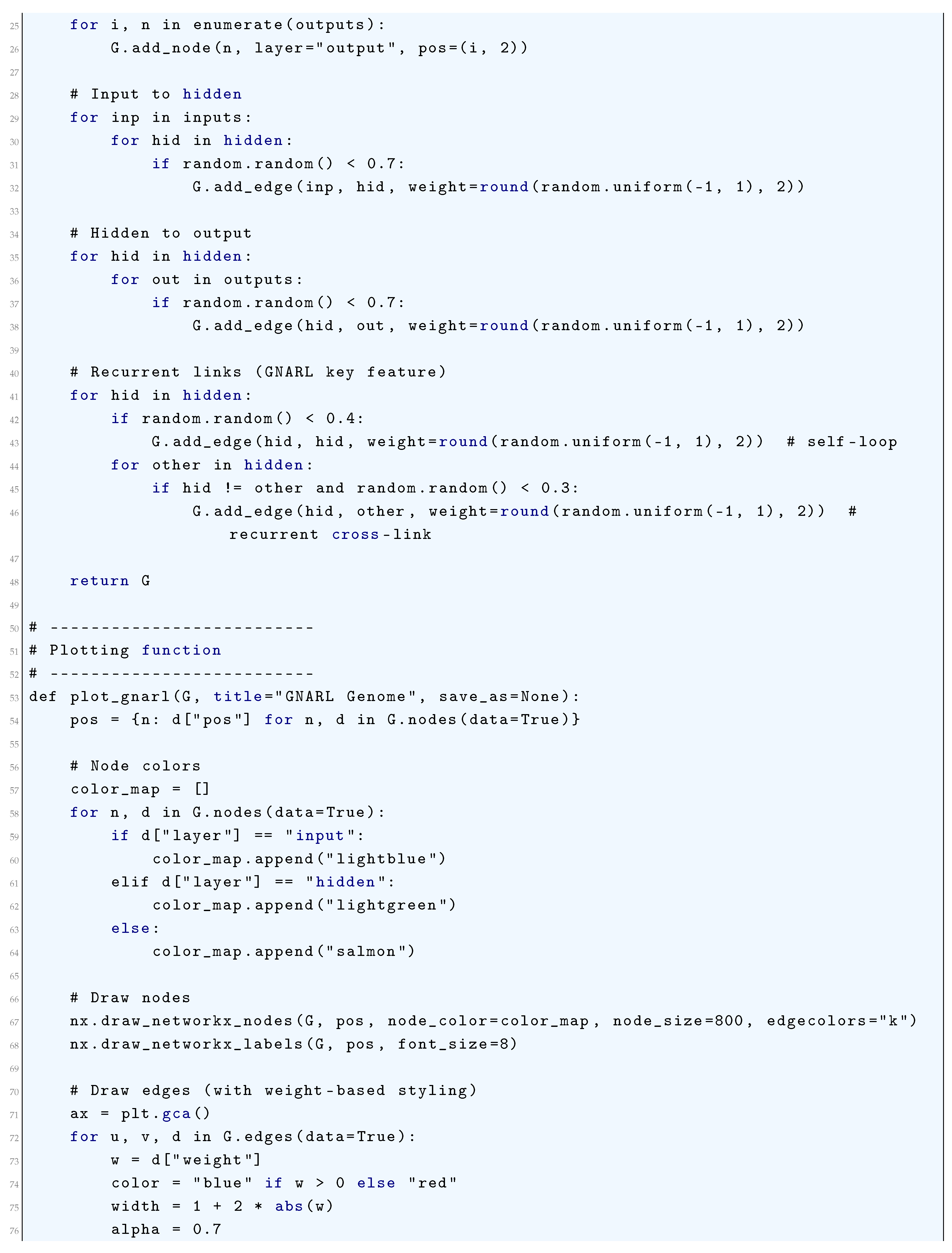
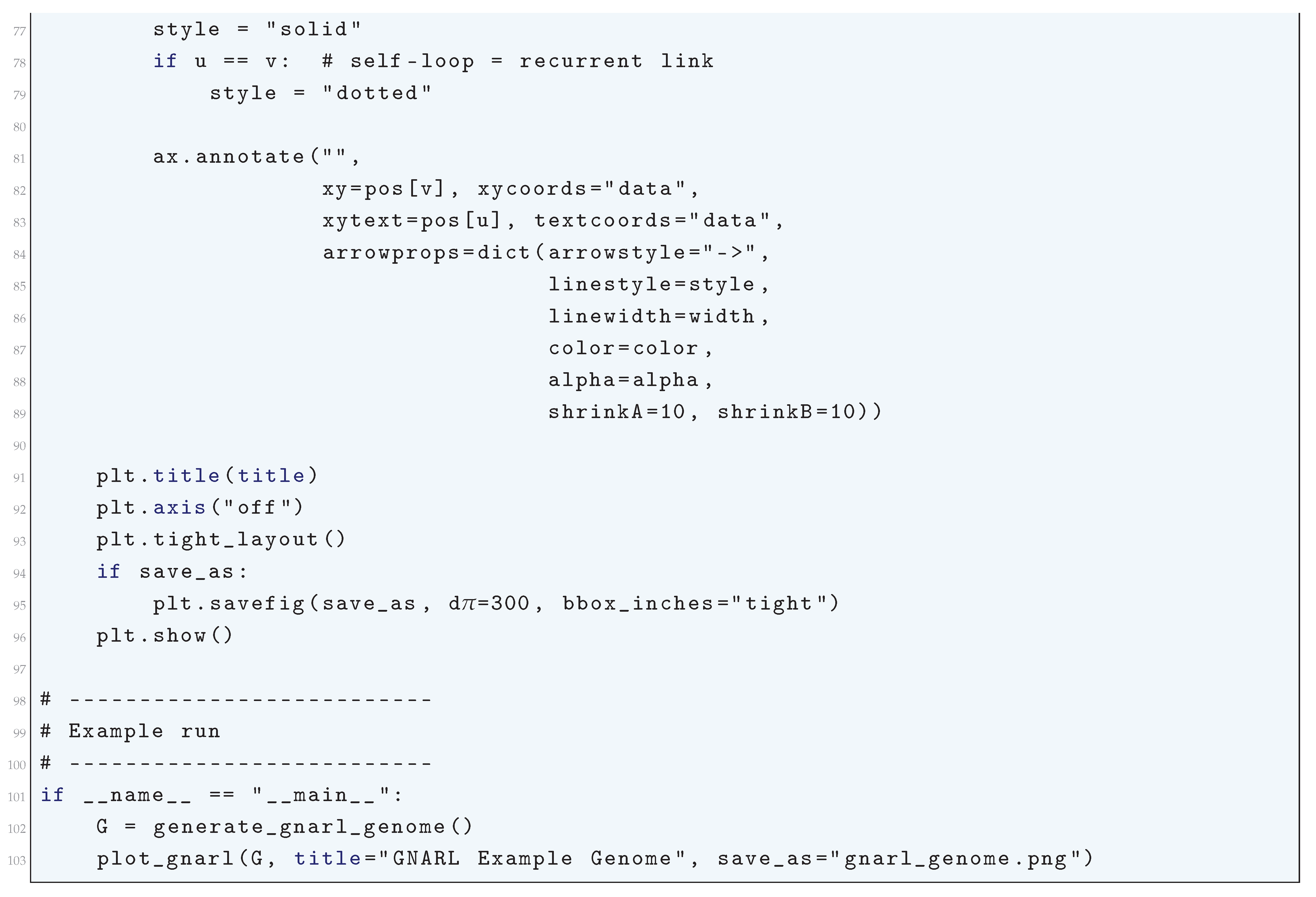
Figure 196.
Visualization of a GNARL (GeNeralized Acquisition of Recurrent Links) genome: Input nodes (blue), hidden nodes (green), and output nodes (red) are shown. Solid arrows represent standard feedforward connections, while dotted arrows indicate recurrent links. Edge color represents sign (blue: positive, red: negative), and thickness is proportional to weight magnitude
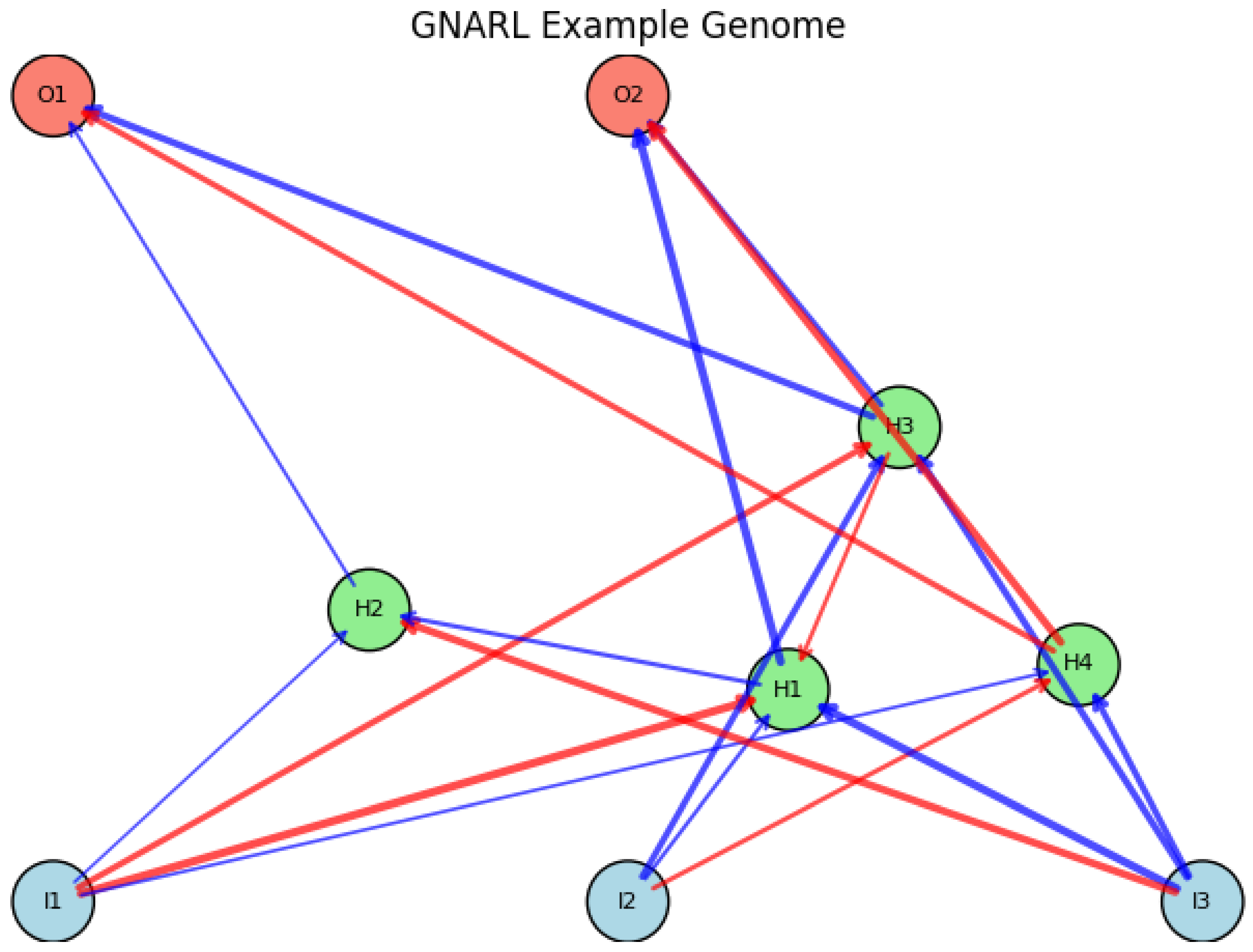
16.5.5. Neuroevolution of Augmenting Topologies (NEAT)
The Neuroevolution of Augmenting Topologies (NEAT) method is a powerful approach in artificial intelligence that applies evolutionary algorithms to optimize both the weights and the topology of artificial neural networks (ANNs). Traditional neuroevolution methods generally evolve fixed-topology networks, limiting their ability to discover innovative structures. NEAT circumvents this limitation by dynamically augmenting network topology, thereby evolving increasingly complex structures while maintaining genetic compatibility through historical markings. Let the genome representation of a neural network be denoted as a directed graph , where the set V consists of input, hidden, and output neurons, and E represents weighted connections between these neurons. Each connection has an associated weight such that the activation of neuron j is given by
where is the set of neurons feeding into neuron j, is the bias term, and is the activation function, which is often chosen to be a non-linear function such as the sigmoid
or a rectified linear unit (ReLU)
In NEAT, the evolutionary process begins with a population of simple neural networks (often with only input and output layers) and progressively adds new connections and new neurons via mutation operations.
The weight evolution follows a traditional genetic algorithm, where mutations modify the connection strengths:
where is the learning rate and is a Gaussian noise term. Structural mutations can add a new connection between two previously unconnected nodes with a probability , or a new node can be inserted into an existing connection with probability . The insertion of a new node replaces an edge with two edges and , and their weights are initialized as
One of the central innovations of NEAT is the use of historical markings to track the lineage of genes (connections). Each connection gene is assigned an innovation number upon creation, which remains unchanged throughout evolution. The similarity d between two genomes and is computed using the genetic distance metric
where E is the number of excess genes, D is the number of disjoint genes, W is the average weight difference of matching genes, and are scaling coefficients. The normalization factor N accounts for genome length to prevent excessive penalties for larger networks. This metric is crucial for implementing speciation, where similar networks are grouped into species to encourage innovation without being prematurely eliminated by competition. The fitness of each network G is evaluated using a task-dependent function , and species-level fitness sharing is applied to maintain diversity:
where is a step function that determines whether two genomes belong to the same species:
with being a speciation threshold. Networks within a species compete primarily amongst themselves, fostering the survival of innovative structures. The crossover operation between two parent genomes and is performed by inheriting matching genes randomly and retaining excess and disjoint genes from the more fit parent:
where is the genome with the higher fitness. If a connection gene in one parent is disabled due to mutation, it is inherited in a disabled state unless reactivated by future mutations. Another fundamental aspect of NEAT is complexification, wherein networks start minimally and gradually increase in complexity by adding nodes and connections. Unlike fixed-topology methods, NEAT allows evolution to discover increasingly sophisticated representations, leading to efficient problem-solving. The network complexity at generation t is measured by
where and denote the number of neurons and connections, respectively. Over time, the structural complexity increases as new mutations introduce novel architectures. In practice, the evolutionary process iterates until convergence, defined by an optimal fitness threshold such that
The mutation rates and are typically annealed to balance exploration and exploitation, governed by
where are decay rates. In summary, NEAT dynamically evolves both weights and network structures while preserving historical innovations and maintaining diversity through speciation. The key principles—incremental complexification, historical markings, and speciation—enable NEAT to efficiently discover topologies that traditional methods struggle to optimize. The continuous balance between exploration and exploitation, governed by well-defined evolutionary operators, results in a robust and self-adaptive neuroevolution framework.
16.5.5.1 Python Code to Generate Figure 197
The NeuroEvolution of Augmenting Topologies (NEAT) algorithm evolves both the weights and topology of neural networks. A plot for NEAT should show:
- Input, hidden, and output nodes.
- Edges with weights (positive = blue, negative = red).
- Disabled connections (often drawn as dashed or faded).
- Labels showing node IDs.
The Python code below produces the Figure 197 illustrating Neuroevolution of augmenting topologies (NEAT).
Figure 197.
Visualization of a NEAT genome: Input nodes (blue), hidden nodes (green), and output nodes (red) represent the network structure. Connections are colored blue for positive weights and red for negative weights, with thickness proportional to weight magnitude. Enabled connections are shown as solid arrows, while disabled ones are dashed
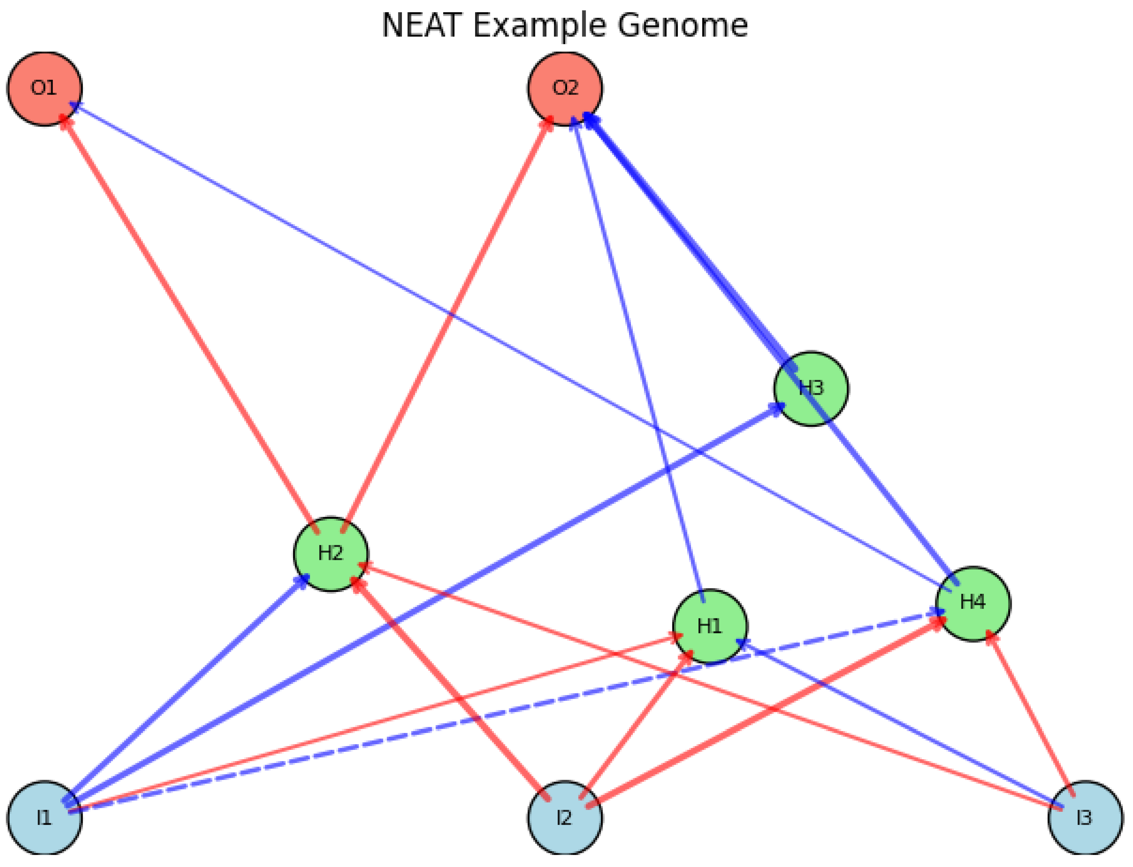
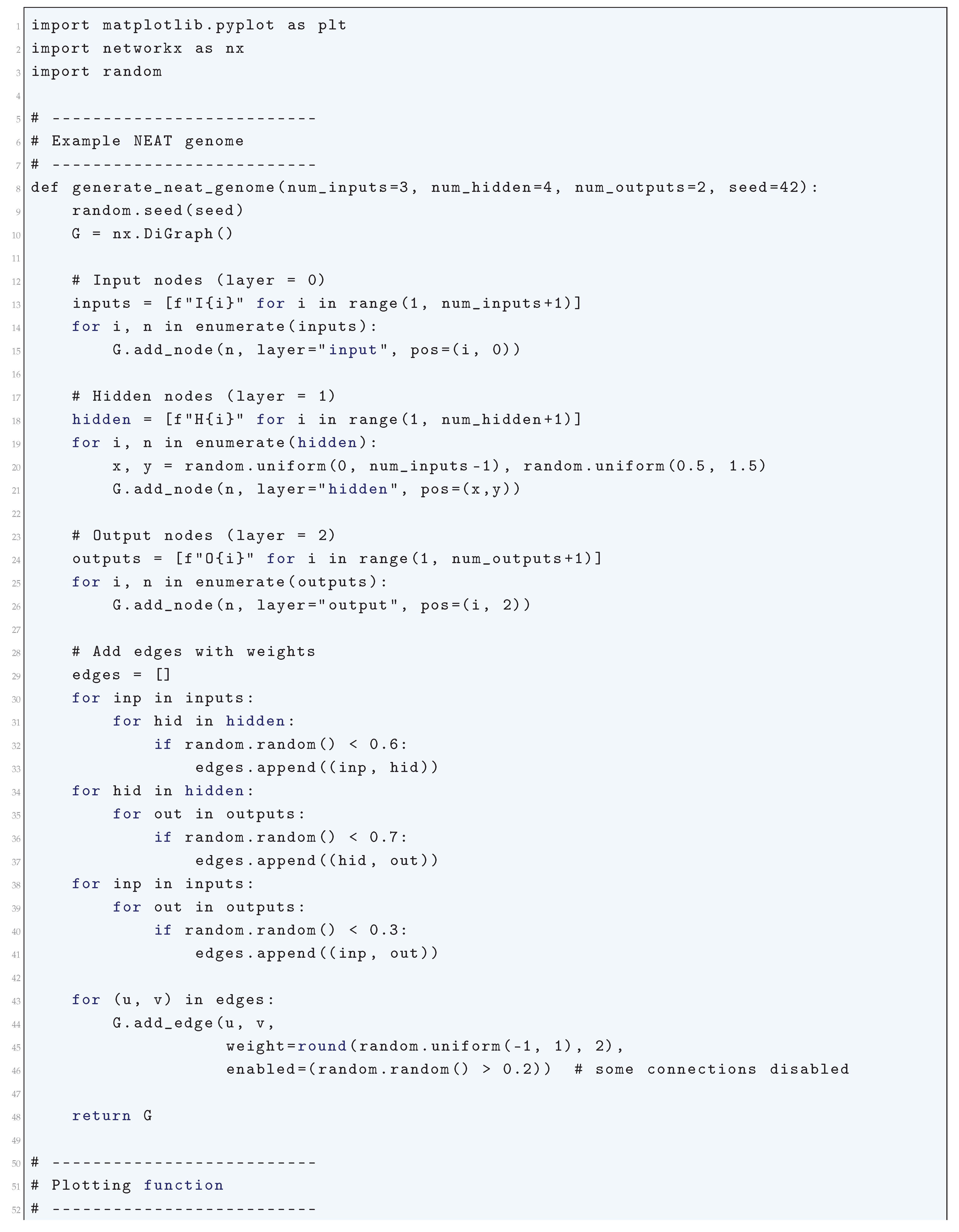
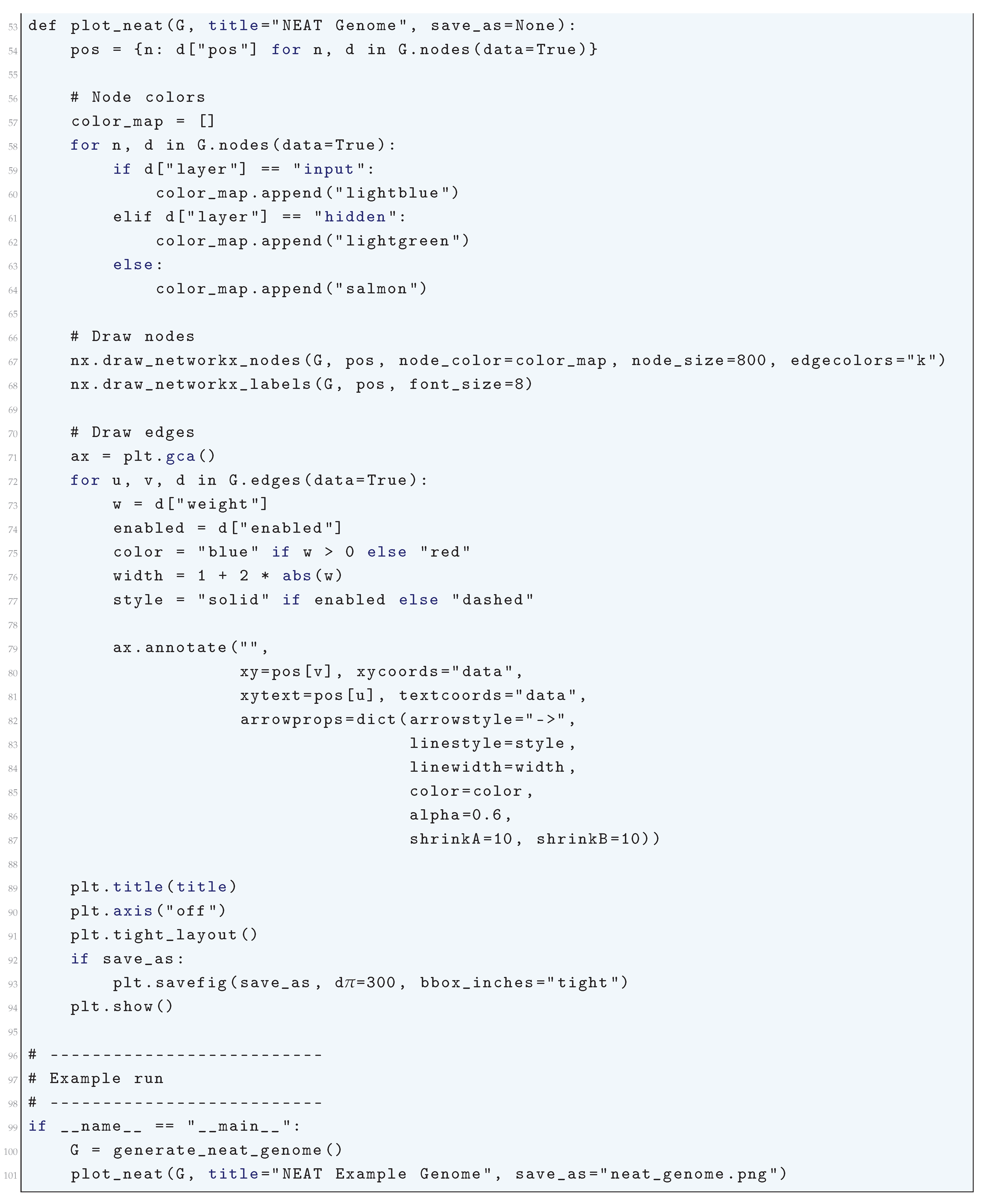
16.5.6. Hypercube-Based NeuroEvolution of Augmenting Topologies (HyperNEAT)
The Hypercube-based NeuroEvolution of Augmenting Topologies (HyperNEAT) method is a neuroevolutionary approach that extends the NeuroEvolution of Augmenting Topologies (NEAT) algorithm by leveraging a Compositional Pattern Producing Network (CPPN) to encode the connectivity patterns of artificial neural networks (ANNs) through a substrate. The fundamental idea behind HyperNEAT is to exploit geometric regularities in the problem domain by encoding the connectivity of a neural network as a function of spatial coordinates, allowing it to generate large-scale neural structures with intricate connectivity patterns in a computationally efficient and evolutionarily scalable manner.
Mathematically, let the neural substrate be defined as a set of nodes embedded in a D-dimensional Euclidean space, where each node is assigned a spatial coordinate . The weight matrix W of the neural network is not directly evolved but rather generated dynamically using a function that maps the spatial positions of node pairs to connection weights. This function f is instantiated by a Compositional Pattern Producing Network (CPPN), which is a fully connected feedforward neural network with activation functions that can include sigmoidal, Gaussian, sine, and identity functions, among others. The connectivity weight between two neurons located at coordinates and is given by:
where the function is parameterized by the weights and activation functions of the CPPN, which itself undergoes neuroevolution using the NEAT algorithm. The CPPN represents a compressed encoding of the connectivity pattern, which allows the network to exploit spatial regularities in a way that would be infeasible with a direct encoding approach. The NEAT algorithm evolves the CPPN by mutating and recombining genomes, where each genome G represents a set of neurons and connections forming the CPPN. A genome G in the NEAT representation consists of a set of node genes and a set of connection genes, where each connection gene is represented as a tuple:
where i and j are node indices, is the connection weight, and enabled is a binary flag indicating whether the connection is active. The fitness function that guides the evolution is determined by the performance of the decoded ANN on the given task. The evolution proceeds using mutation operators such as:
where is a Gaussian perturbation, and structural mutations that add nodes and connections, preserving the historical marking mechanism of NEAT. Once the CPPN is evolved, it is queried at every pair of spatial coordinates in the neural substrate to generate the weight matrix:
where S is the set of nodes in the substrate. This procedure ensures that the evolved ANN inherits the geometric properties encoded by the CPPN, leading to topological coherence and the ability to scale up efficiently. The substrate structure can be fixed or evolved, leading to a variety of architectures including multi-layer perceptrons, convolutional-like structures, and even more complex topologies. The implicit encoding provided by the CPPN enables patterned connectivity with symmetries, repetitions, and other motifs that are biologically plausible and computationally advantageous. HyperNEAT’s search space is thus fundamentally different from traditional neuroevolution approaches, as it searches over functions that encode networks rather than over networks themselves. This means that small changes in the CPPN can lead to large, structured modifications in the ANN’s connectivity, a property known as indirect encoding. Formally, the space of networks N encoded by a CPPN is given by:
where f is constrained by the activation functions and weight structure of the CPPN. The expressiveness of the encoding is controlled by the activation functions in the CPPN, which determine the nature of the patterns it can represent. A significant advantage of HyperNEAT is its ability to exploit domain regularities by leveraging geometric relationships within the substrate. For example, in a vision-based task, neurons representing nearby pixels should have stronger connections, which can be captured by a distance-sensitive function:
where and are evolved parameters that control the strength and scale of connectivity. This equation ensures that neurons form meaningful topologies based on spatial structure. HyperNEAT optimizes the encoding function rather than individual weights, allowing it to generalize connectivity patterns across different domains and tasks. This ability to evolve topological regularities has been successfully applied in robot control, game playing, function approximation, and large-scale pattern recognition.
16.5.6.1 Python Code to Generate Figure 198
HyperNEAT generates neural networks by mapping a geometric substrate via a CPPN.
- Nodes are in a 2D (or 3D) substrate.
- Connections are determined by the CPPN, usually sparse but patterned.
-
Visualization should highlight:
- (a)
- Node positions (substrate coordinates)
- (b)
- Connection weights (width proportional, color by sign)
The Python code below produces the Figure 198 illustrating Hypercube-based NeuroEvolution of Augmenting Topologies (HyperNEAT).
Figure 198.
Visualization of a HyperNEAT substrate-based neural network: Input nodes (blue), hidden nodes (green), and output nodes (red) are positioned in a geometric substrate. Edge thickness is proportional to weight magnitude, with blue representing positive weights and red representing negative weights
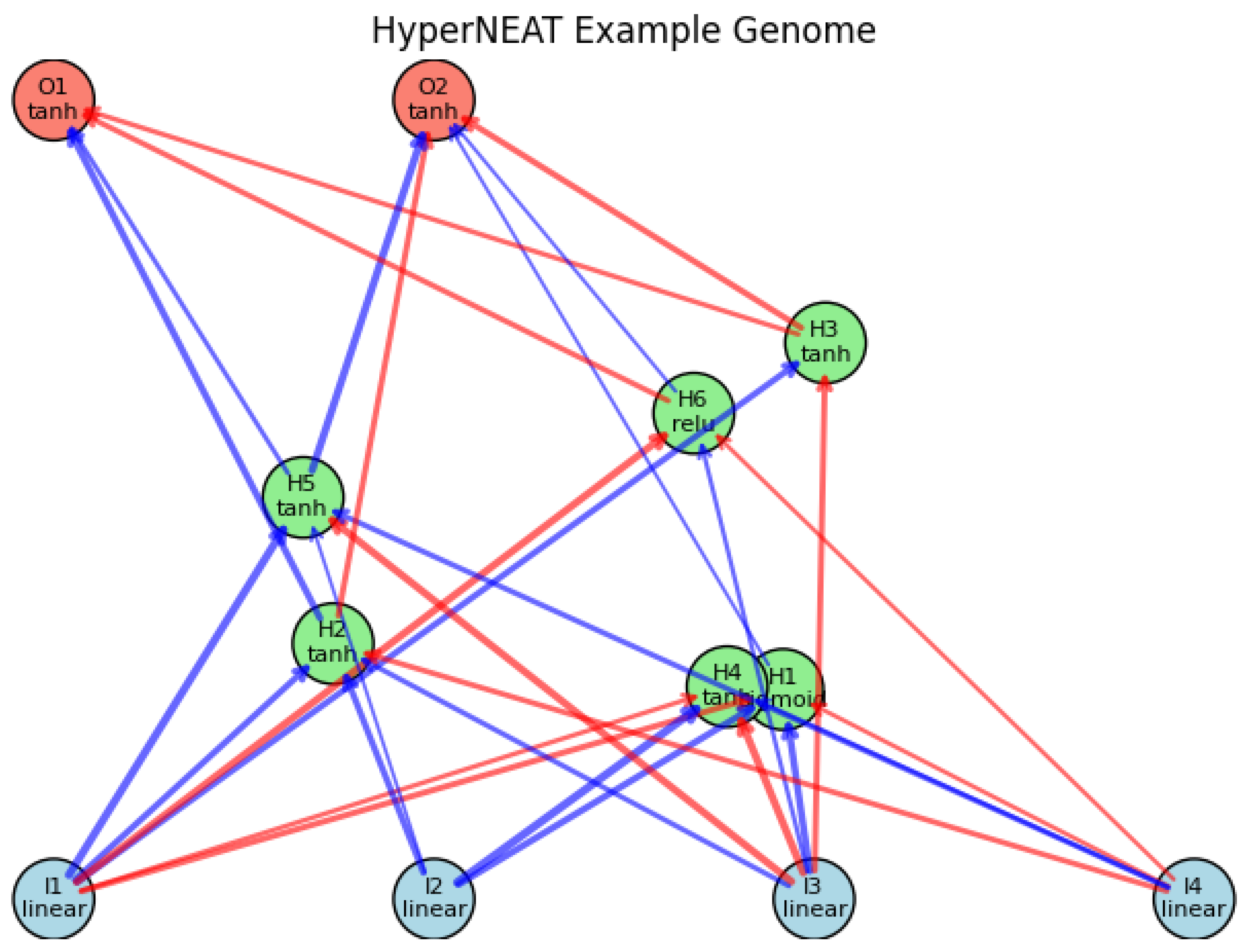
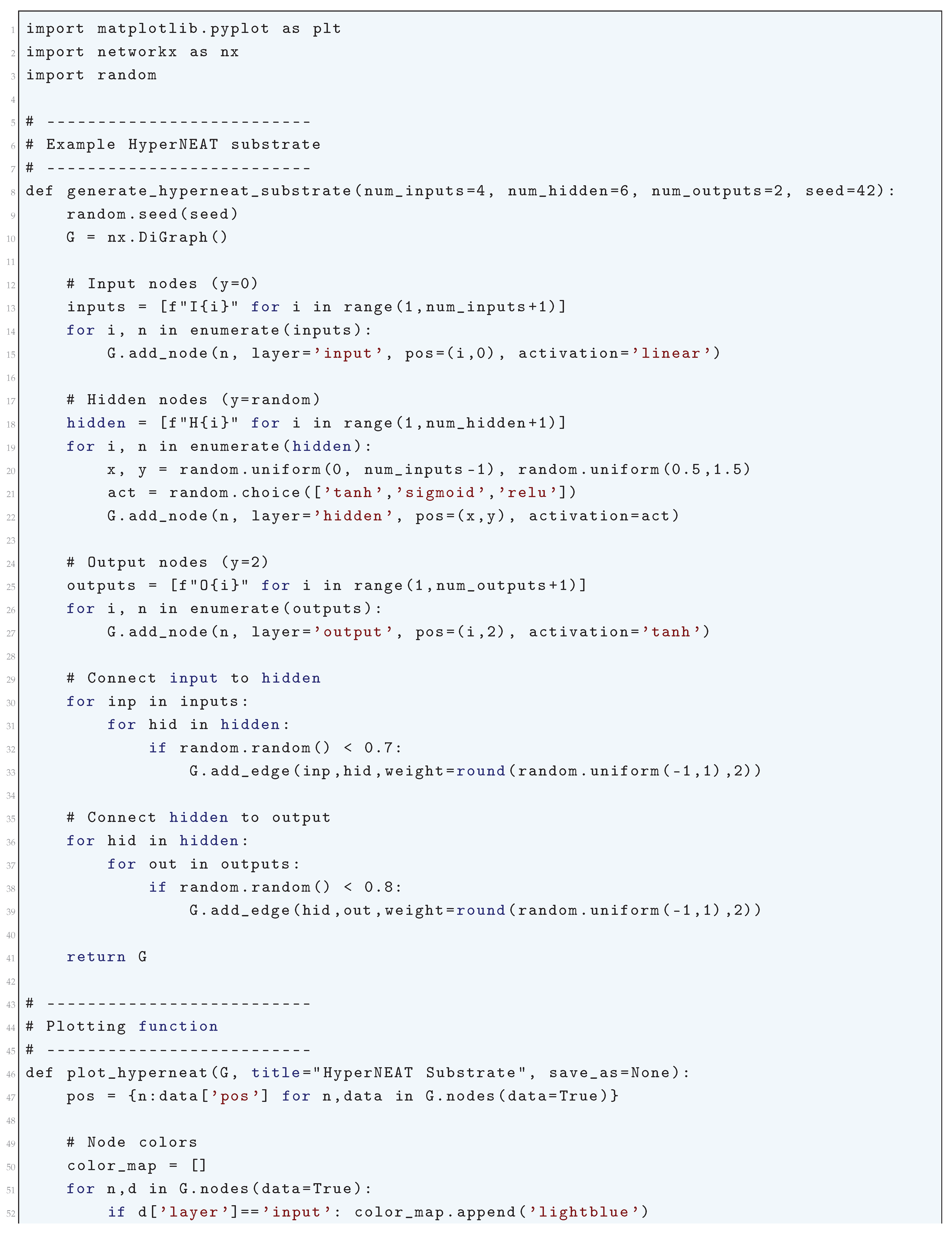
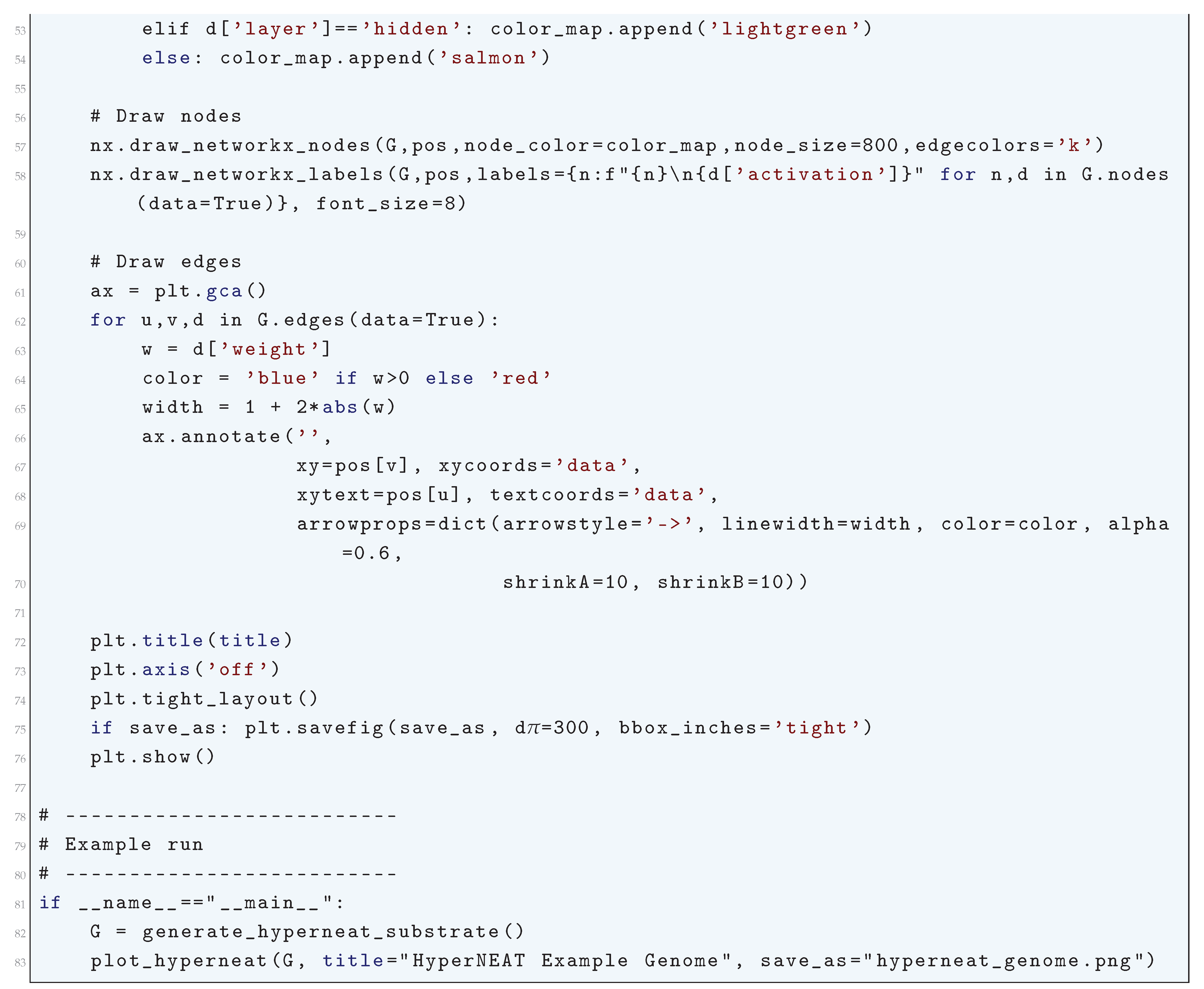
16.5.7. Evolvable Substrate Hypercube-Based NeuroEvolution of Augmenting Topologies (ES-HyperNEAT)
The Evolvable Substrate Hypercube-based NeuroEvolution of Augmenting Topologies (ES-HyperNEAT) method is an advanced extension of the Hypercube-based NeuroEvolution of Augmenting Topologies (HyperNEAT) algorithm, which itself is based on NeuroEvolution of Augmenting Topologies (NEAT). The fundamental premise of ES-HyperNEAT is the encoding of connectivity patterns in neural networks using Compositional Pattern-Producing Networks (CPPNs), which are evolved through genetic algorithms. This approach allows for the indirect encoding of large-scale artificial neural networks (ANNs) by leveraging geometric regularities and adaptive connectivity growth to discover task-relevant neural substrates in a computationally efficient manner.
The ES-HyperNEAT methodology extends HyperNEAT by evolving connectivity patterns based on local fitness evaluations within a neural substrate, rather than relying on global constraints alone. The key innovation in ES-HyperNEAT is the ability to discover and refine important network regions dynamically, without explicitly requiring a predefined topology. Given a substrate space with spatial coordinates for nodes , the connection strength between two nodes is encoded by a functionally evolved CPPN, represented mathematically as
Here, is a neural network that encodes the weights between nodes based on their spatial location. The CPPN is evolved via NEAT, which optimizes its parameters and topology to generate increasingly complex connectivity patterns. Unlike conventional ANN weight optimization, which directly evolves individual weights, ES-HyperNEAT leverages the implicit regularities in the substrate to determine connections based on geometric principles. To formally describe the weight expression process, let us define the CPPN-generated weight function as a mapping:
A fundamental property of this mapping is substrate symmetry, which is captured by the fact that weight magnitudes for symmetric inputs in the domain follow similar functional properties:
This symmetry allows for computational efficiency, as only a fraction of the connections need to be explicitly evaluated. In ES-HyperNEAT, unlike conventional HyperNEAT, the adaptive growth mechanism is introduced by defining an adaptive threshold function over the substrate, which dynamically determines whether a connection should be expressed. The connection viability is determined by:
where is a learned function that varies over the substrate space and is itself evolved during the learning process. The introduction of adaptive thresholds enables ES-HyperNEAT to selectively prune redundant connections while preserving the essential connectivity for task-relevant computation. The neural network instantiated from the CPPN-generated substrate follows a typical activation dynamics governed by the weighted sum and activation function:
where is the activation of node i, is the synaptic weight from node j to node i, is a bias term, and is a nonlinear activation function (e.g., sigmoid, tanh, or ReLU). The ES-HyperNEAT approach further refines the weight refinement strategy by incorporating a local function-based weight refinement, denoted as , which modifies the initial weights W using a learned adaptive function :
This refinement process iteratively enhances connectivity by reinforcing important regions in the substrate while eliminating weak connections through thresholding and weight decay. The effect is a progressively optimized connectivity pattern that dynamically adapts to the learning environment. From a mathematical perspective, the evolution of the CPPN itself follows genetic mutation and crossover dynamics, where the genetic encoding of the CPPN, denoted by , undergoes variation through mutation functions and crossover functions :
Here, t represents the generation index, and and are the CPPN parameters of parent solutions selected based on fitness evaluations. The fitness function F evaluates the network’s performance on a given task and is defined as:
where is a loss function comparing predicted outputs to true labels . The evolutionary process seeks to maximize F, leading to increasingly optimized neural architectures. Overall, the ES-HyperNEAT approach represents a mathematically rigorous framework for evolving complex neural network topologies through adaptive connectivity growth, thresholded weight refinement, and neurogenesis-driven substrate expansion. The resulting architectures are not only topologically optimized but also computationally scalable, making ES-HyperNEAT a powerful tool for the evolution of high-dimensional neural representations in artificial intelligence.
16.5.7.1 Python Code to Generate Figure 199
ES-HyperNEAT generates large-scale neural networks by evolving substrates and connection patterns via Compositional Pattern Producing Networks (CPPNs).
- Nodes are arranged in a geometric substrate (usually 2D or 3D).
- Connections are created based on the CPPN output across node coordinates.
- Visualizations typically show:
- Node positions in substrate (x, y).
- Weighted connections (colored by sign, thickness by magnitude).
The Python code below produces the Figure 200 illustrating Evolvable Substrate Hypercube-based NeuroEvolution of Augmenting Topologies (ES-HyperNEAT).
Figure 199.
Visualization of an ES-HyperNEAT substrate-based neural network: Input nodes (blue), hidden nodes (green), and output nodes (red) are positioned in a geometric substrate. Edge thickness is proportional to weight magnitude, with blue representing positive weights and red representing negative weights
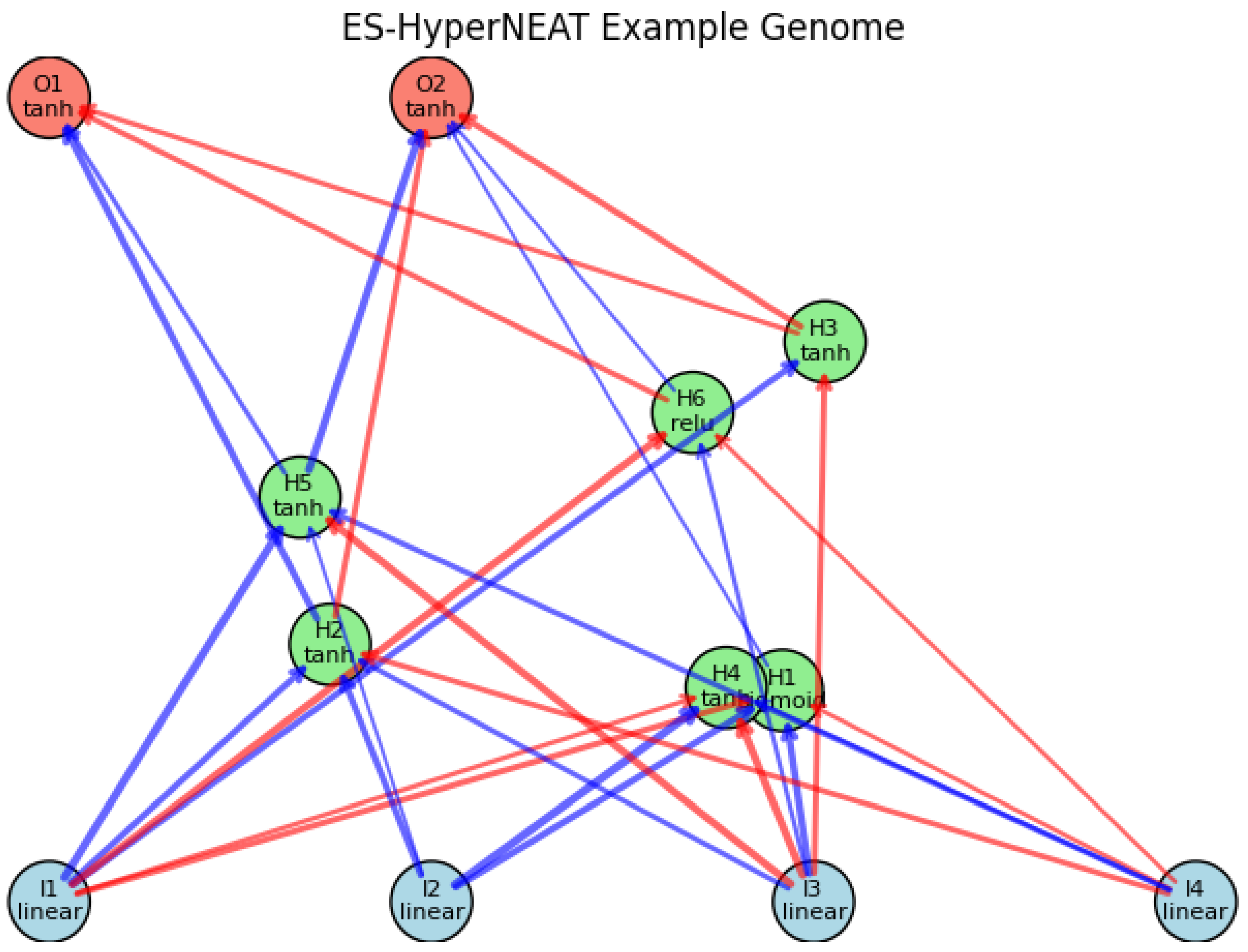
Figure 200.
Visualization of the Evolutionary Acquisition of Neural Topologies (EANT2): Input nodes (blue), hidden nodes (green), and output nodes (red) form an evolved topology. Edge colors represent weights (blue: positive, red: negative) with thickness proportional to magnitude
Figure 200.
Visualization of the Evolutionary Acquisition of Neural Topologies (EANT2): Input nodes (blue), hidden nodes (green), and output nodes (red) form an evolved topology. Edge colors represent weights (blue: positive, red: negative) with thickness proportional to magnitude
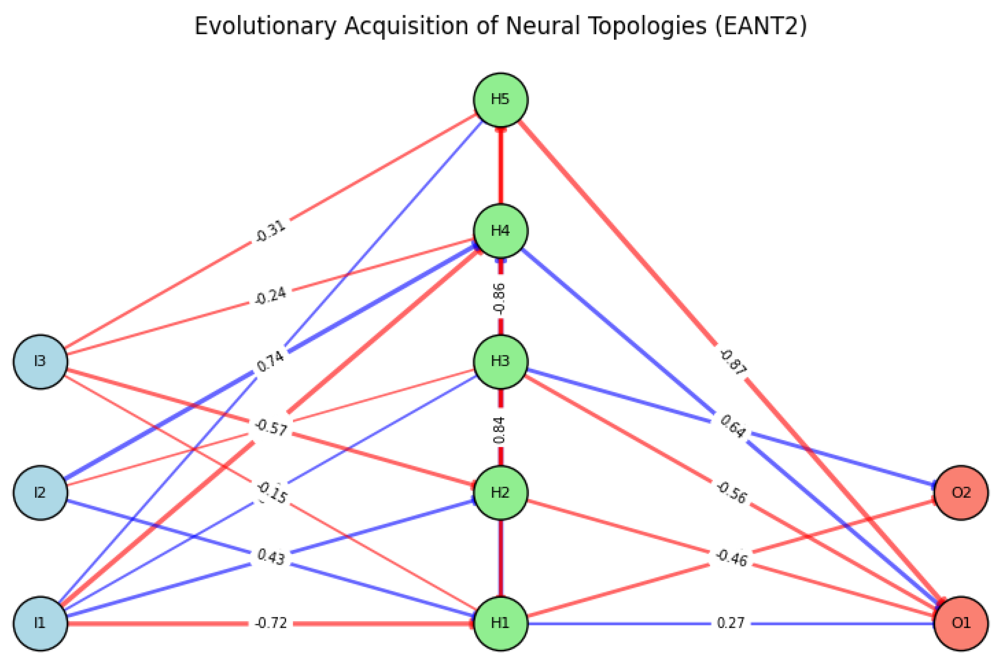
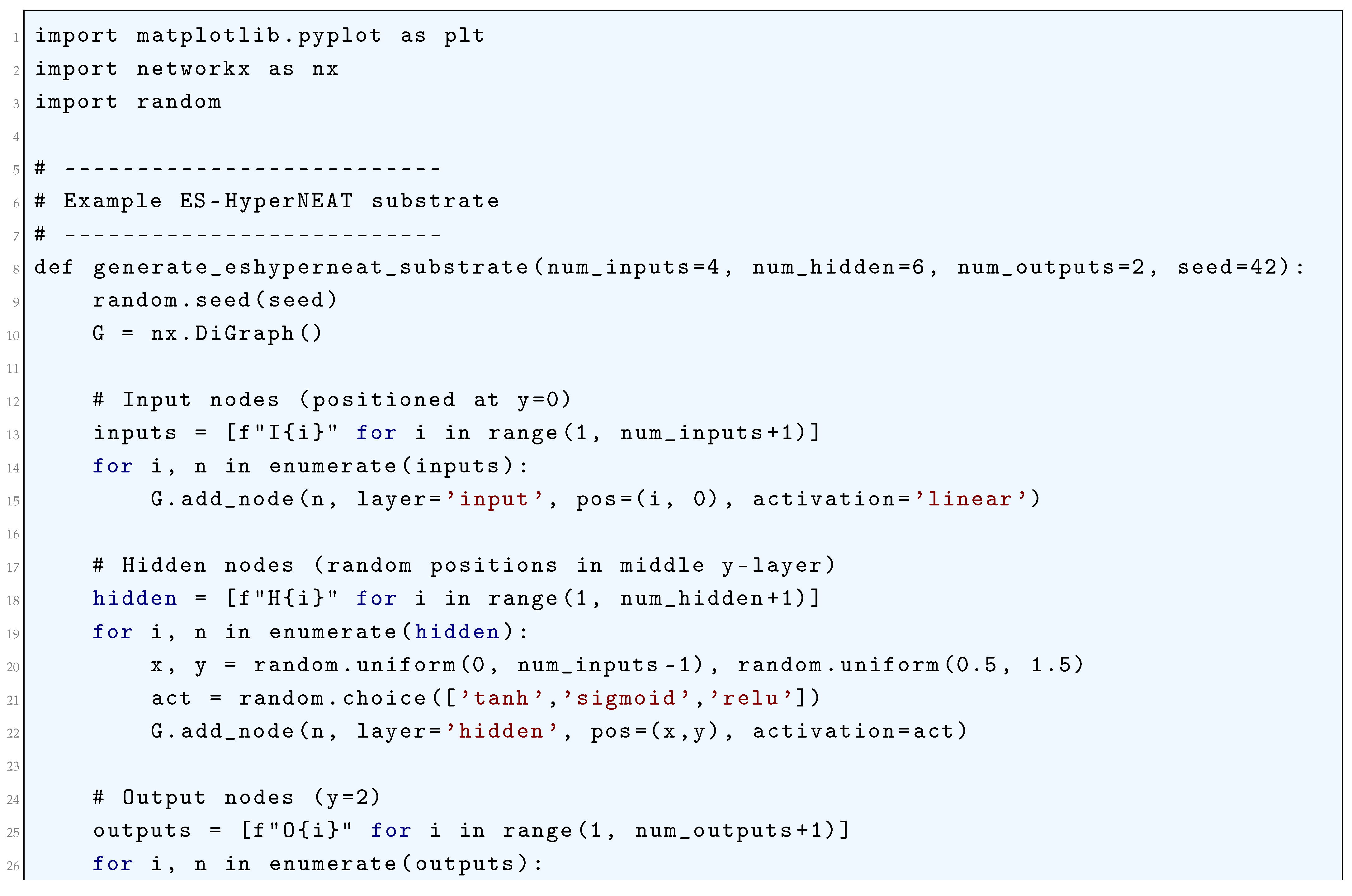
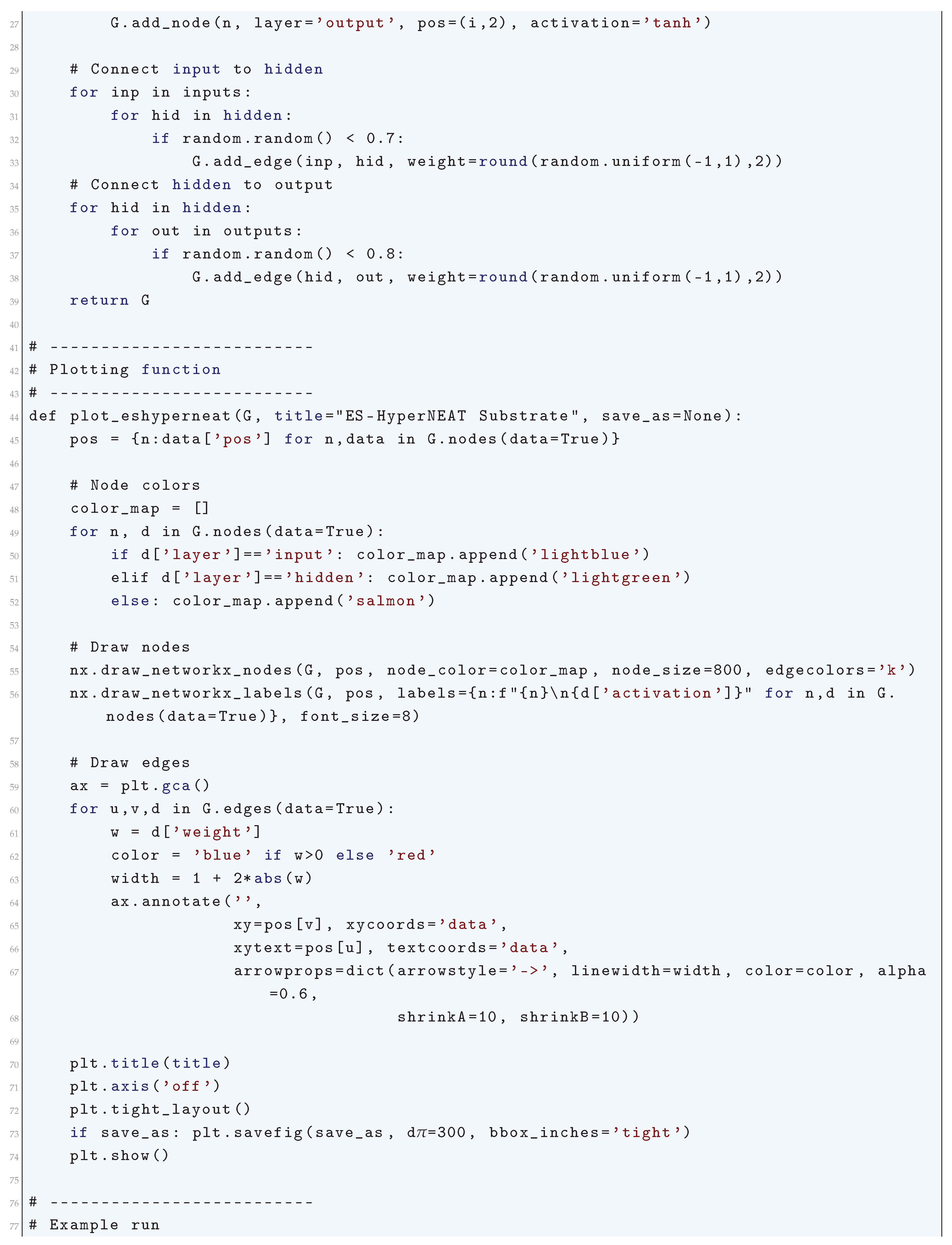
16.5.8. Evolutionary Acquisition of Neural Topologies (EANT/EANT2)
Literature Review: EANT has been assessed on multiple benchmark tasks, such as the RoboCup keepaway challenge (Metzen et. al. (2007) [986]) and the double-pole balancing problem (Kassahun and Sommer 2005 [987]), consistently achieving high performance. A more advanced version, EANT2, was later introduced and tested on a visual servoing task, where it surpassed both the traditional iterative Gauss–Newton method and NEAT (Siebel and Sommer [988]). Additional experiments have also been conducted to evaluate its capabilities in classification problems (Siebel and Sommer [990]).
Recent Literature Review:
The Evolutionary Acquisition of Neural Topologies (EANT) and its extension EANT2 are advanced methods for evolving artificial neural networks (ANNs) through an evolutionary process that simultaneously optimizes both the topology and the weights of the network. The primary principle underlying EANT/EANT2 is the combination of evolutionary algorithms (EAs) and neural network training, allowing for the automatic discovery of optimal network architectures without the need for manual design. The method begins with an initial minimal structure and progressively complexifies through mutations and recombinations, ensuring efficient exploration of the search space while avoiding unnecessary complexity. A neural network in the context of EANT/EANT2 can be defined as a directed graph , where the set of vertices V represents neurons, and the set of edges E represents synaptic connections. Each edge carries an associated weight , which modulates the signal transmission from neuron i to neuron j. Mathematically, the activation of neuron j at time step t is given by:
where denotes the set of presynaptic neurons to j, are the connection weights, is the bias term, and is the activation function, typically chosen as the sigmoid function
or the hyperbolic tangent function
In the EANT framework, network evolution begins with a set of simple neural networks containing only input and output neurons, with hidden neurons introduced incrementally via evolutionary operators.
The evolution of network topology is governed by genetic operators such as mutation and crossover. Mutation can involve perturbing connection weights, adding or deleting neurons, or modifying the topology in a more structured manner. The mutation of a weight follows a Gaussian perturbation model:
where is a Gaussian-distributed random variable with mean zero and variance , and is a learning rate parameter. The selection process follows a fitness-based evaluation, where each neural network in a population is assigned a fitness score based on its performance on a given task. The selection probability of an individual network follows a Boltzmann distribution:
where is a temperature parameter controlling selection pressure. EANT2 extends EANT by introducing covariance matrix adaptation (CMA) for more efficient weight optimization. In CMA, the evolution of the weight vector is guided by a covariance matrix , which dynamically adapts to the topology of the search landscape. The weight update rule in EANT2 is given by:
where is the identity matrix. The covariance matrix is updated using an evolution path formulation:
where is a learning rate, and is the evolution path. Throughout the evolutionary process, EANT/EANT2 ensures that only structurally beneficial changes are retained, leading to an efficient exploration-exploitation tradeoff. The incremental growth of topology in EANT can be mathematically formalized by defining the probability of adding a new neuron as
where represents the fitness improvement from the structural modification, and is a control parameter. At each iteration, the population of neural networks undergoes selection, mutation, and recombination, leading to the formation of an improved generation. The optimization objective is to maximize a performance metric , where represents the training dataset. The overall evolutionary update rule can be expressed as
where is a learning rate and the second term represents stochastic exploration. The convergence of EANT/EANT2 is governed by the stability of the weight adaptation dynamics. If the eigenvalues of the Jacobian matrix
lie within the unit circle, the evolutionary process stabilizes, ensuring convergence. Otherwise, further structural modifications are required to regularize the topology. Thus, EANT/EANT2 provides a mathematically rigorous framework for evolving neural networks by simultaneously optimizing topology and weights, leveraging evolutionary principles, and incorporating efficient weight adaptation techniques such as CMA. The fundamental strength of the method lies in its ability to construct minimal yet powerful architectures that efficiently learn complex functions.
16.5.8.1 Python Code to Generate Figure 200
The Evolutionary Acquisition of Neural Topologies (EANT) algorithm evolves neural network topologies using evolutionary strategies. A plot should show:
- Input layer, hidden nodes, output layer.
- Evolved connections (weighted, possibly sparse).
- Mutations such as added nodes or connections.
- Generation info (to highlight evolutionary growth).
The Python code below produces the Figure 200 illustrating Evolutionary Acquisition of Neural Topologies (EANT) algorithm.
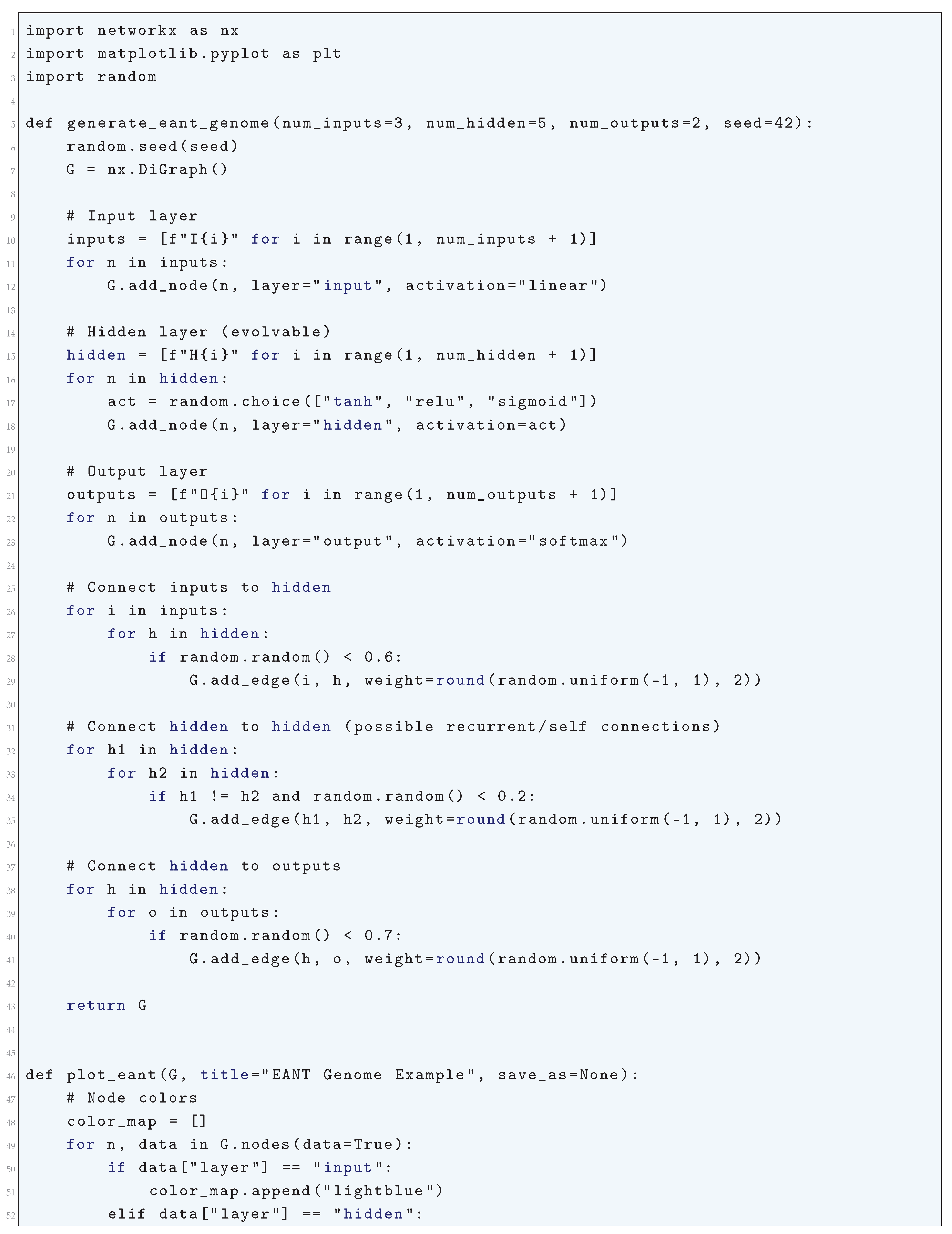
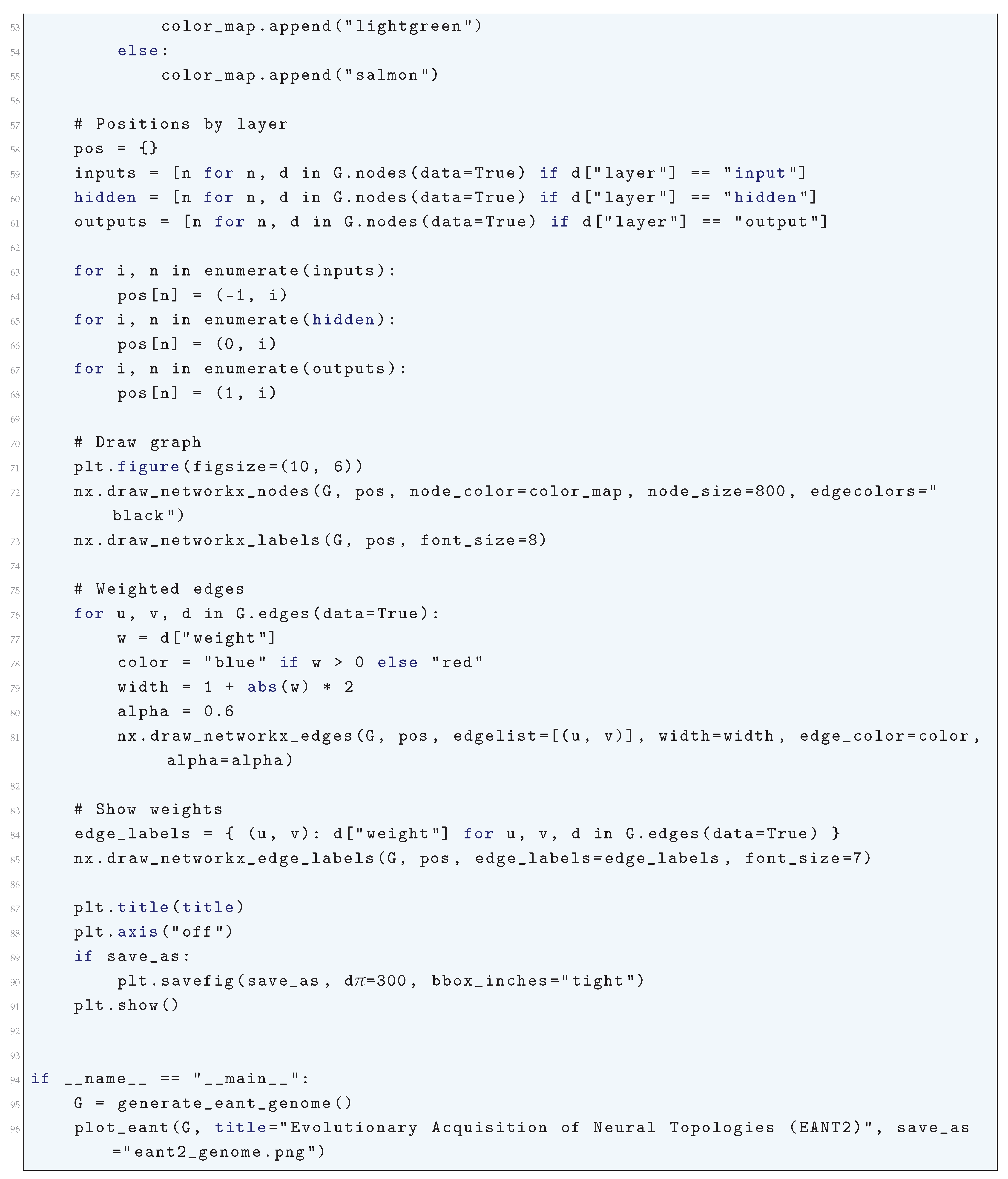
16.5.9. Interactively Constrained Neuro-Evolution (ICONE)
The Interactively Constrained Neuro-Evolution (ICONE) method in artificial intelligence is a sophisticated approach that integrates interactive constraints into neuro-evolutionary algorithms to refine the optimization of neural networks. This method combines evolutionary strategies with constraint-driven feedback mechanisms, ensuring the evolution process adheres to a set of dynamically imposed mathematical and computational constraints. The evolution of neural network architectures and weights follows a rigorously constrained adaptation process, driven by feedback mechanisms that enforce both explicit and implicit constraints.
Neuro-evolution optimizes the weights and structures of artificial neural networks using evolutionary algorithms. Consider a neural network parameterized by a weight vector , where n is the number of trainable parameters. The loss function of the network, denoted as , defines the objective landscape in which evolutionary search occurs. The ICONE method introduces interactive constraints that enforce adherence to specific functional, structural, or performance-based criteria, which we define mathematically as
where represents the ith constraint function, ensuring the evolved network satisfies predefined conditions. The evolution process follows a mutation-selection cycle under constrained optimization. Given an initial population at generation t, candidate solutions undergo mutation:
where is a perturbation vector sampled from an isotropic Gaussian distribution with variance . The feasibility of each mutated candidate is determined by evaluating the constraints . If a candidate violates any constraints, a projection step enforces feasibility by solving the constrained optimization problem:
This ensures that every evolved individual remains within the feasible search space. Selection in ICONE is governed by fitness evaluation and constraint satisfaction. The fitness function incorporates both performance metrics (e.g., classification accuracy, regression error) and constraint penalties. A penalty-based fitness function is formulated as:
where is a penalty coefficient enforcing constraint satisfaction. Higher fitness candidates are selected for reproduction, forming the next generation . A key characteristic of ICONE is interactive constraint adaptation, where constraints evolve dynamically based on intermediate feedback. If the optimization process trends toward infeasible solutions, adaptive constraints are imposed by modifying the constraint functions:
where is an adaptation rate controlling the magnitude of constraint adjustment. This adaptation mechanism ensures the evolutionary process remains both stable and effective, guiding solutions toward desirable regions in the search space. The convergence of ICONE relies on satisfying the Karush-Kuhn-Tucker (KKT) conditions, which characterize optimality in constrained optimization. At convergence, optimal solutions satisfy the Lagrangian formulation:
where are the Lagrange multipliers. The necessary conditions for optimality are:
These conditions ensure the final neural network configuration is both performance-optimized and constraint-compliant.
Ultimately, the ICONE method provides a mathematically rigorous framework for constrained neuro-evolution, ensuring neural networks evolve under explicit, dynamically adaptable, and interactive constraints while maintaining optimal performance in their designated tasks. Through a constraint-driven evolutionary search, ICONE guarantees that evolved models satisfy both functional and theoretical constraints, leading to robust and interpretable artificial intelligence systems.
16.5.9.1 Python Code to Generate Figure 201
Interactively Constrained Neuro-Evolution (ICONE) is a neuroevolution framework where:
- The user (human-in-the-loop) constrains evolution by enforcing rules (e.g., disallow certain connections, force modularity, or bias toward certain structures).
- Architectures evolve under both evolutionary pressure and interactive constraints.
-
Visualization should therefore highlight:
- (a)
- Neurons and their types.
- (b)
- Connections (weights, enabled/disabled).
- (c)
- Constraints applied (e.g., disallowed connections, frozen neurons).
So, in addition to the usual NEAT/SUNA/DXNN-style graph, we need to mark constrained elements (e.g., red crosses on forbidden edges, shaded neurons if frozen). The Python code below produces the Figure 201 illustrating Interactively Constrained Neuro-Evolution (ICONE).
Figure 201.
Visualization of an Interactively Constrained Neuro-Evolution (ICONE) genome: Neurons are colored by type (input, hidden, output). Frozen neurons (under user constraint) are shaded gray. Arrows represent weighted connections (blue for positive, red for negative), with width proportional to weight magnitude. Disabled connections appear faded, and constrained connections are marked with an “X”
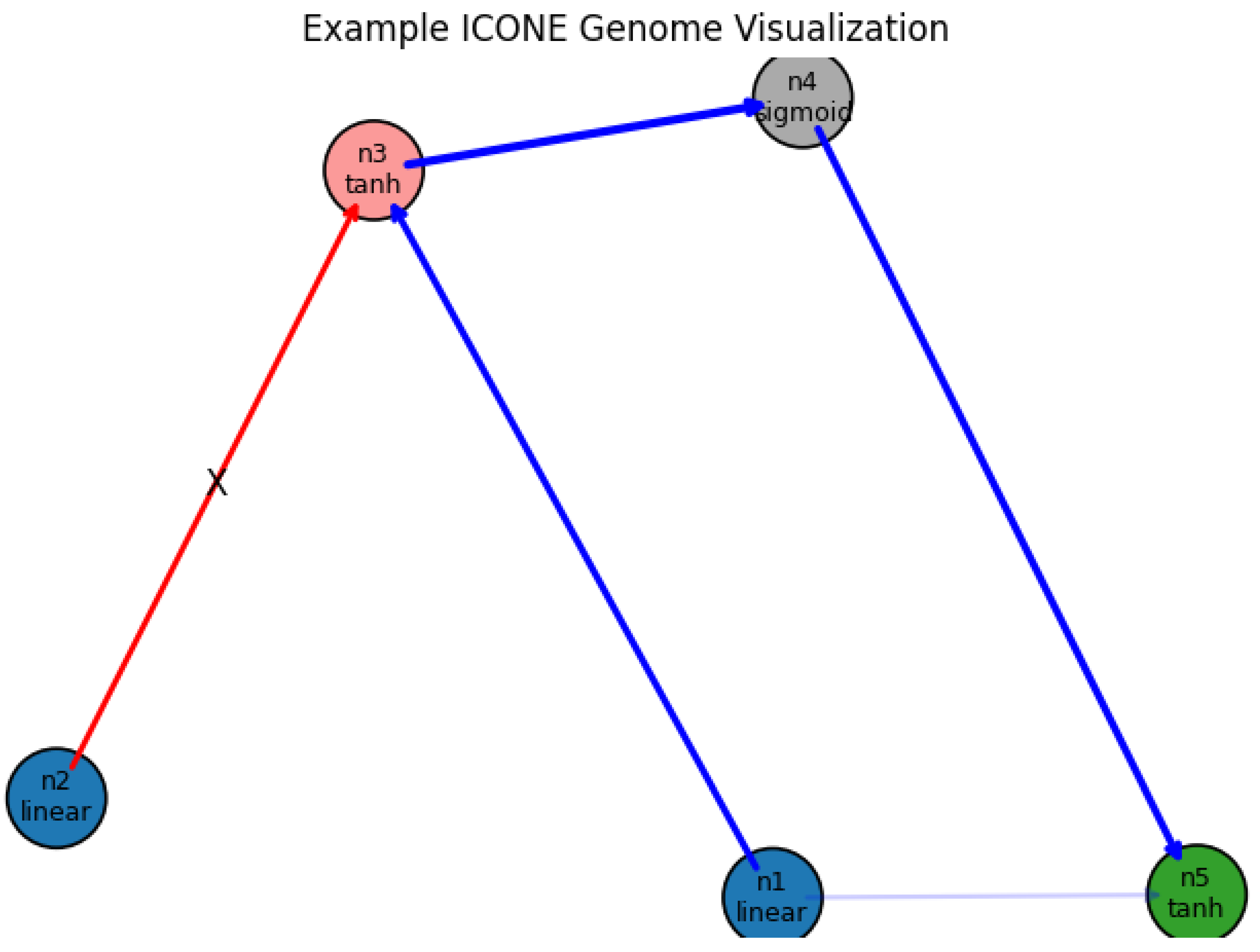

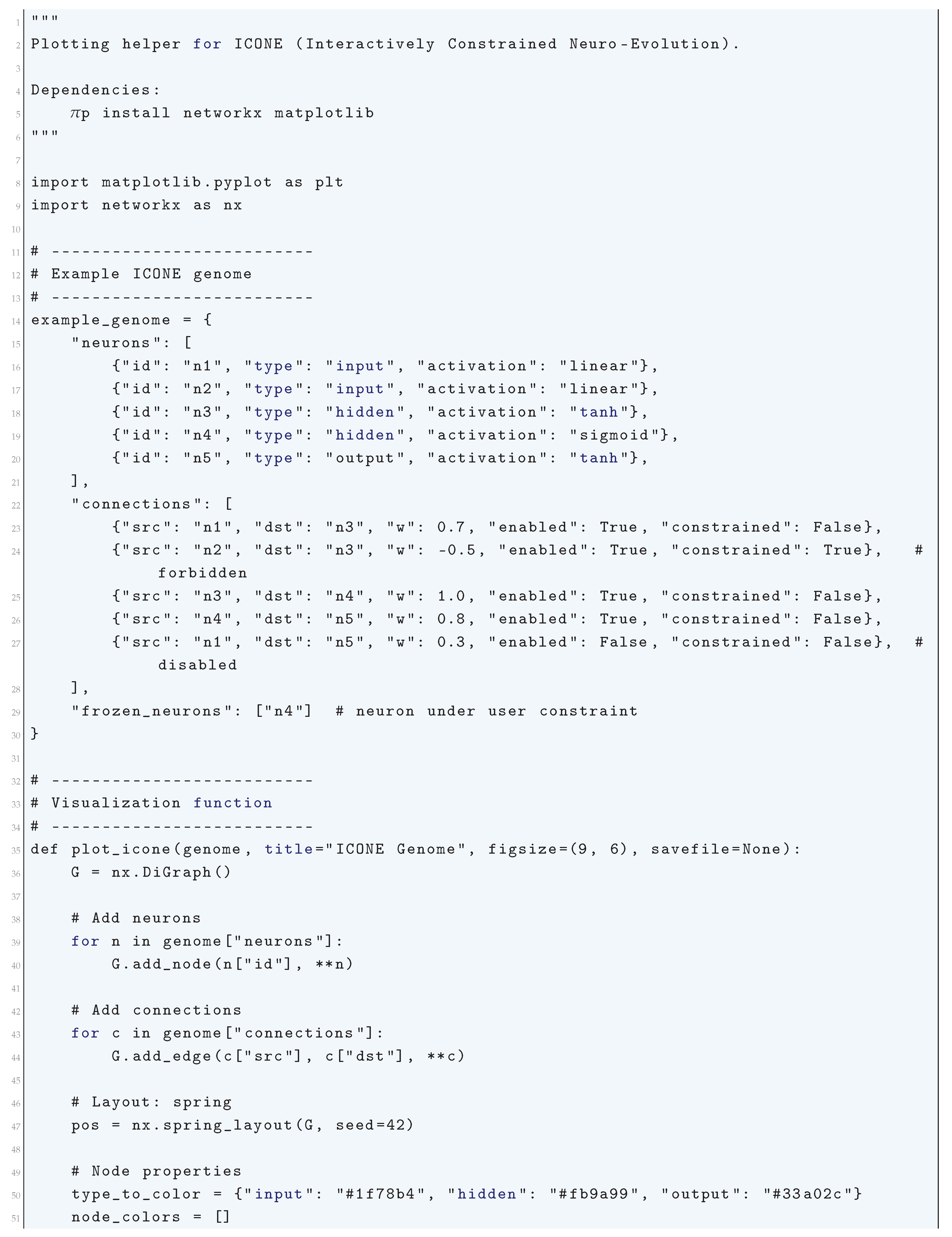
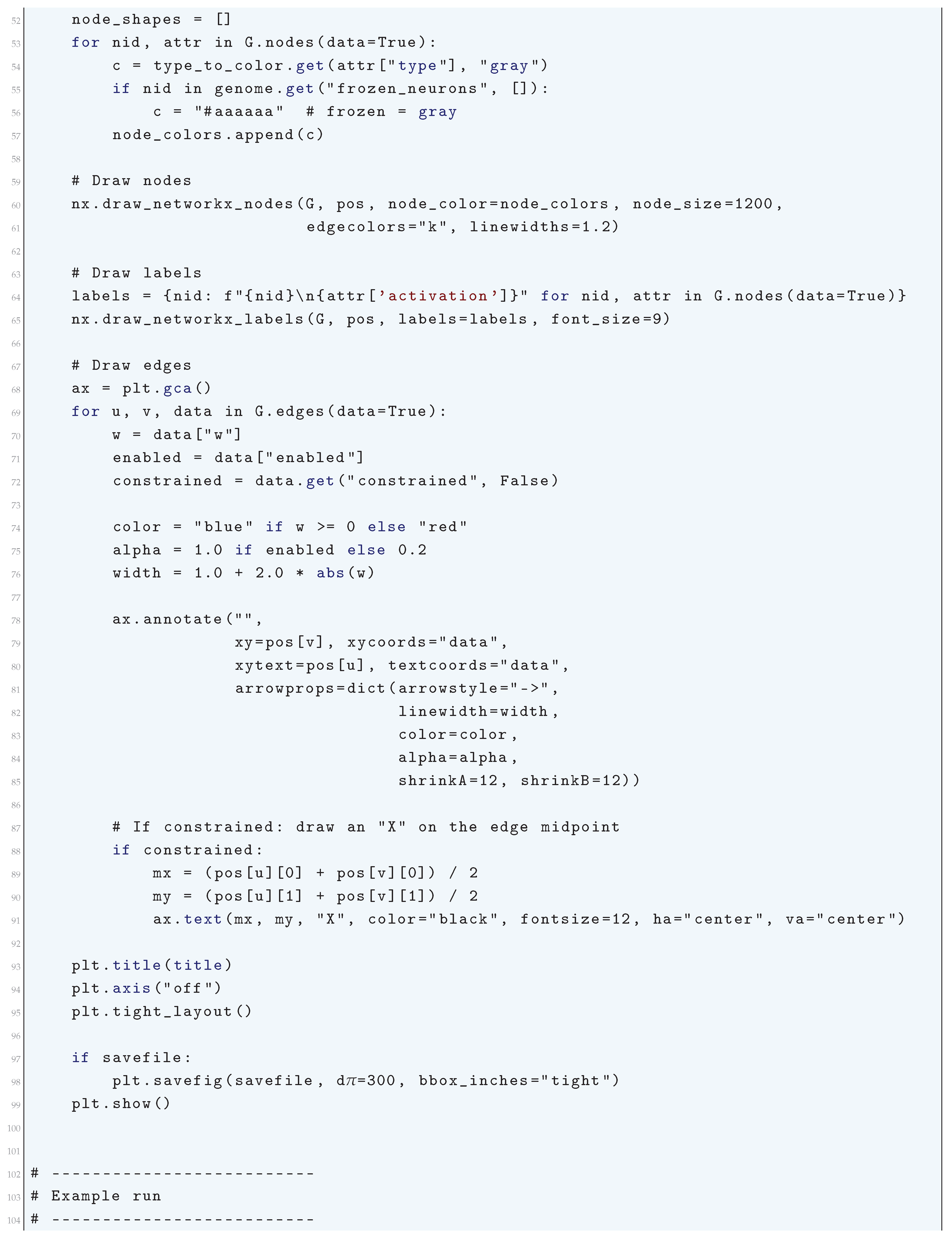
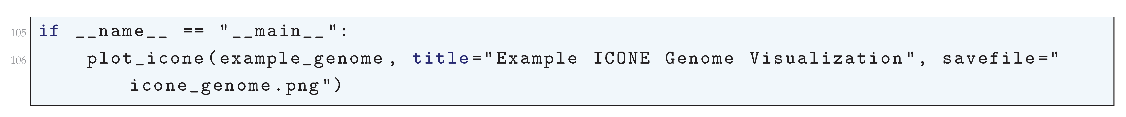
16.5.10. Deus Ex Neural Network (DXNN)
The Deus Ex Neural Network (DXNN) method is a sophisticated approach in artificial intelligence that employs a memetic algorithm-based Topology and Weight Evolving Artificial Neural Network (TWEANN) system. This method is designed to evolve both the structure and parameters of neural networks, enabling the development of models that can adapt to complex tasks without predefined architectures.
In traditional neural network training, the architecture is often fixed, and only the weights are optimized using algorithms like backpropagation. In contrast, DXNN simultaneously evolves the topology and weights of the network. This is achieved through a combination of evolutionary strategies and local search methods, which iteratively refine the network’s performance. The memetic algorithm aspect of DXNN incorporates local optimization techniques within the evolutionary process, enhancing convergence rates and solution quality. Mathematically, the DXNN method can be described as follows:
- Initialization: A population of neural networks is initialized with random topologies and weights. Each network’s topology can be represented as a graph , where V denotes neurons and E denotes synaptic connections.
- Fitness Evaluation: Each network i in the population is evaluated based on a fitness function , which measures its performance on a given task. The fitness function could be defined as:where N is the number of samples, is the true output, is the network’s output, and L is a loss function, such as mean squared error:
- Selection: Networks are selected for reproduction based on their fitness scores. A common selection method is tournament selection, where a subset of networks is chosen, and the one with the highest fitness is selected for reproduction.
- Crossover (Recombination): Pairs of selected networks undergo crossover to produce offspring. This involves combining the topologies and weights of parent networks. For example, given parent networks with weight matrices and , an offspring’s weight matrix could be:where is a crossover coefficient.
- Mutation: Offspring networks undergo mutations to introduce variability. Mutations can affect both the topology and weights. For weight mutation:where is a perturbation matrix, often sampled from a normal distribution:For topology mutation, connections can be added or removed based on a probability or .
- Local Optimization (Memetic Component): After mutation, local search methods, such as gradient-based optimization, are applied to fine-tune the weights of the offspring networks. This involves minimizing the loss function L with respect to the weights W:where is the learning rate, and is the gradient of the loss function with respect to the weights.
- Replacement: The new generation of networks replaces the old population, and the process repeats from the fitness evaluation step until a termination criterion is met, such as a predefined number of generations or a satisfactory fitness level.
The DXNN method has been applied in various domains, including financial markets. For instance, in automated currency trading, DXNN has been used to evolve neural networks that process Forex chart images as inputs, enabling the detection of patterns and trends for trading decisions. This approach contrasts with traditional methods that rely on fixed technical indicators, offering a more dynamic and adaptive trading strategy.
In summary, the Deus Ex Neural Network method provides a comprehensive framework for evolving both the architecture and parameters of neural networks. By integrating evolutionary algorithms with local optimization techniques, DXNN facilitates the development of adaptable and efficient models capable of tackling complex tasks across various domains.
16.5.10.1 Python Code to Generate Figure 202
The Deus Ex Neural Network (DXNN) framework is a modular, hierarchical, evolving neural architecture. It differs from NEAT/SUNA in that: It is hierarchical:
- Neurons form Cores (like sub-networks).
- Cores are grouped into a DXNN organism.
Both neurons and cores can mutate, evolve, and rewire. Visualization should therefore show two levels:
- The Core graph (inter-core connectivity).
- Inside each core, the Neuron graph (intra-core connectivity).
- Cores are grouped into a DXNN organism.
The Python code below produces the Figure 202 illustrating Deus Ex Neural Network (DXNN).
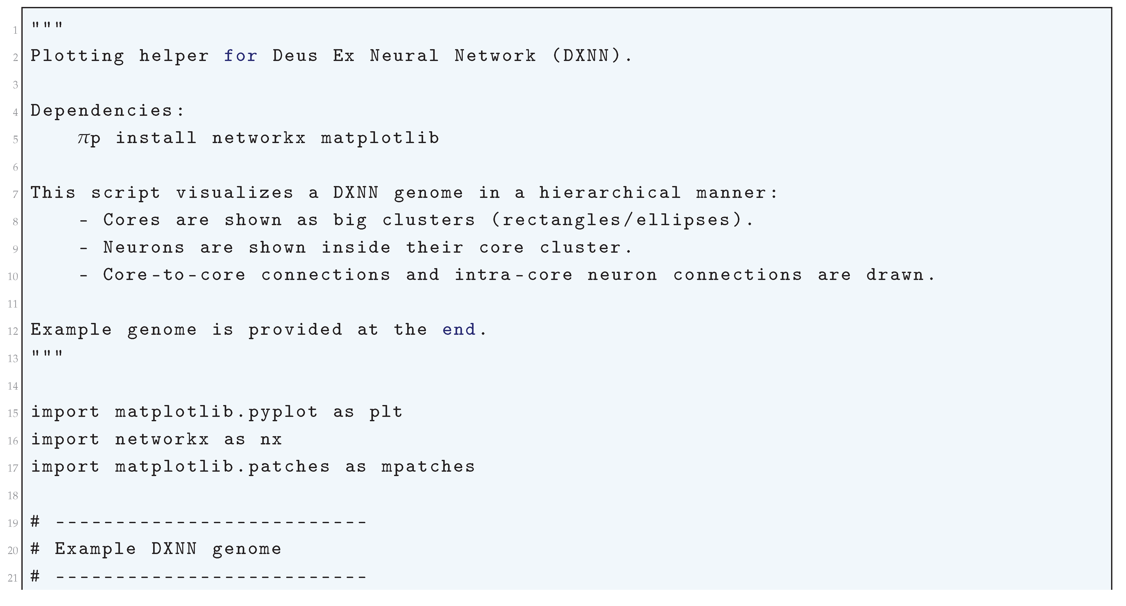
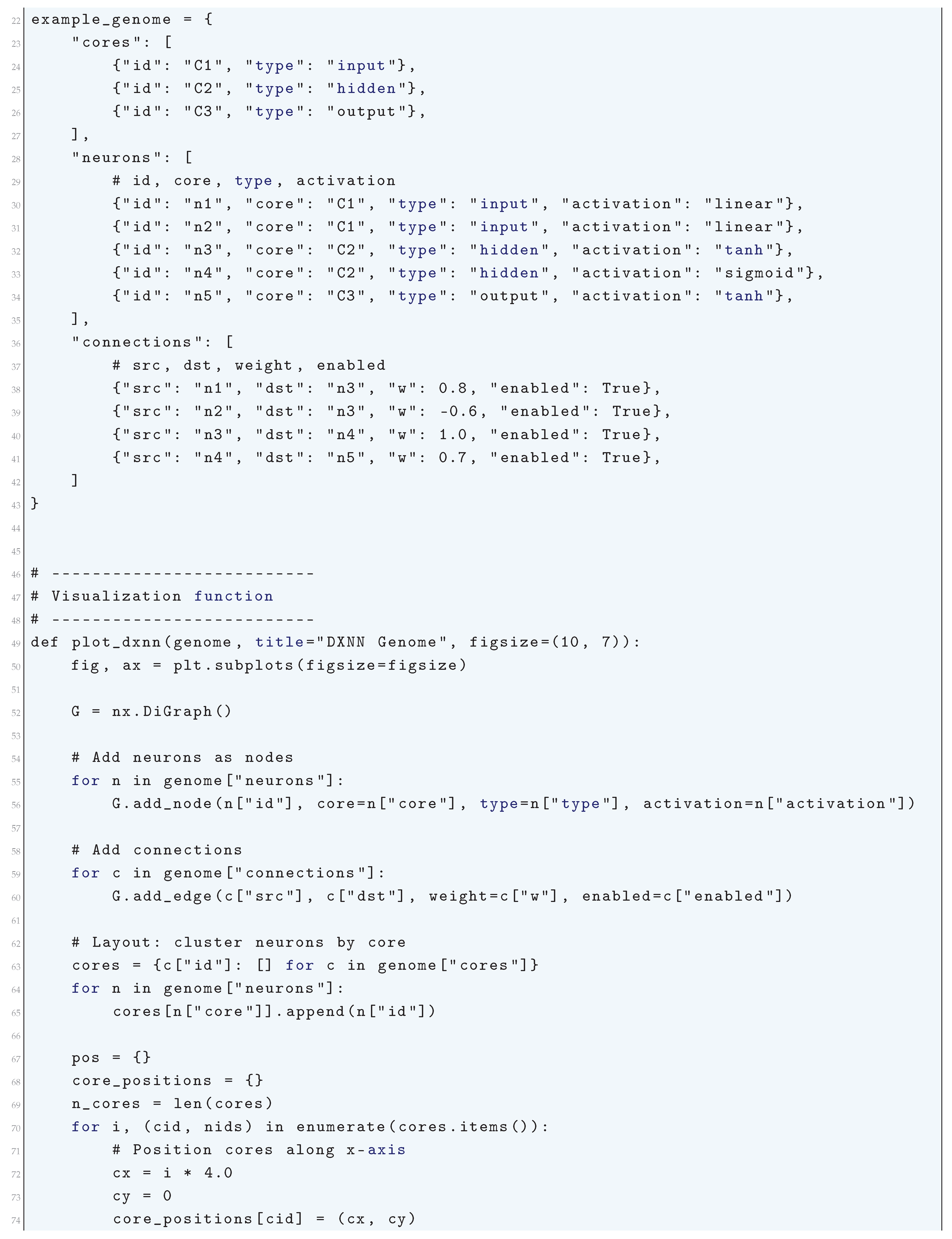
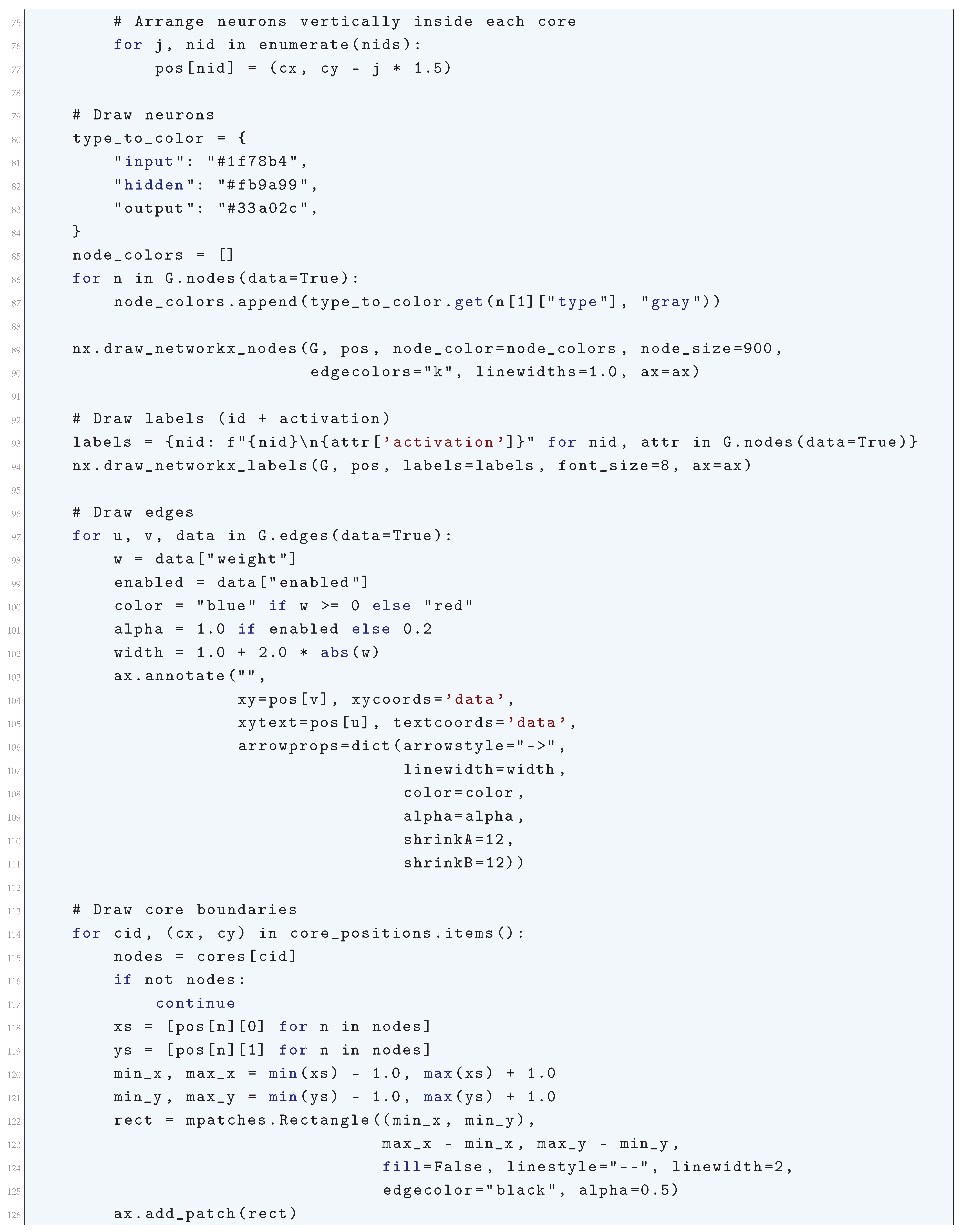
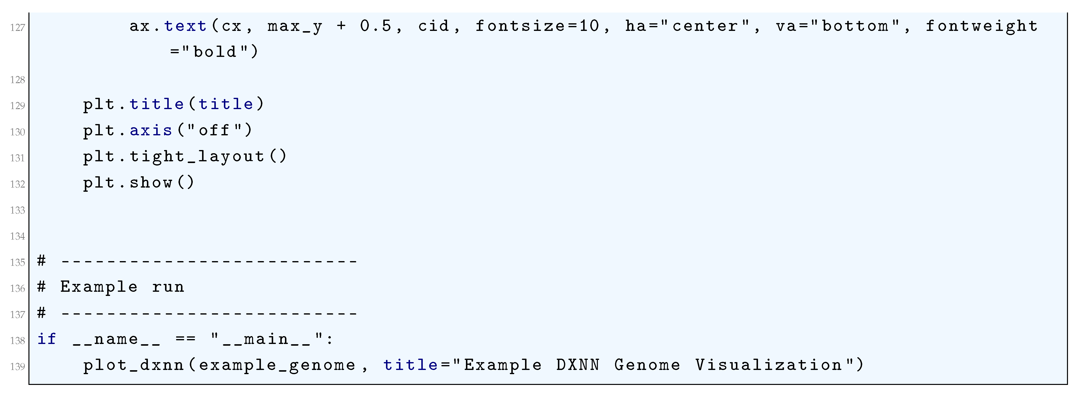
Figure 202.
Visualization of a Deus Ex Neural Network (DXNN) genome. Neurons are grouped into cores (dashed rectangles), colored by type (input, hidden, output). Arrows represent weighted connections (blue for positive, red for negative), with line thickness proportional to weight magnitude. Disabled connections appear faded. Each neuron label indicates its identifier and activation function.
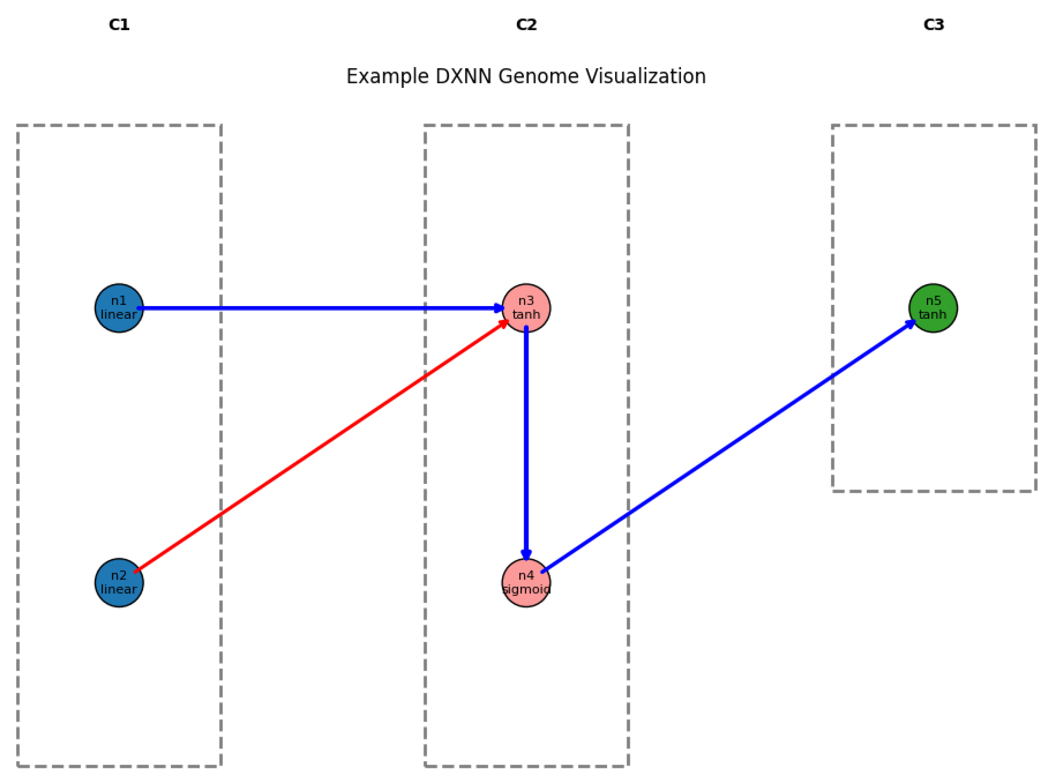
16.5.11. Spectrum-Diverse Unified Neuroevolution Architecture (SUNA)
The Spectrum-diverse Unified Neuroevolution Architecture (SUNA) is an advanced framework in artificial intelligence that synergistically combines a unified neural representation with a novel diversity-preserving mechanism known as spectrum diversity. This integration facilitates the evolution of neural networks with both adaptable topologies and weights, enabling the system to proficiently address a wide array of complex tasks.
Central to SUNA is the Unified Neuron Model, which encapsulates various neuron types and activation functions within a single, cohesive representation. Each neuron i is characterized by a set of parameters , governing its specific function. The output of neuron i can be mathematically expressed as:
Here, denotes the activation function, represents the synaptic weight between neurons j and i, signifies the input from neuron j, and is the bias term associated with neuron i. This formulation allows for the seamless integration of diverse neuronal behaviors within a unified framework.
The evolutionary process in SUNA involves the optimization of both the neural network’s architecture and its synaptic weights. A population of candidate solutions, each encoded as a chromosome C, undergoes iterative selection, crossover, and mutation operations. The fitness of each chromosome is evaluated based on its performance on the target task. The mutation operators are designed to modify the network’s topology and weights, introducing variations that enhance the search for optimal solutions. To maintain a rich diversity of solutions, SUNA employs the spectrum diversity mechanism. This approach constructs a spectrum for each chromosome, capturing its unique characteristics. The spectrum is defined as:
where represents the k-th feature of the chromosome C. The distance D between two spectra and is computed using a suitable metric, such as the Euclidean distance:
This distance metric informs the niching mechanism, ensuring that the evolutionary process explores a diverse set of solutions by promoting chromosomes with unique spectra. The fitness evaluation in SUNA is augmented by a novelty score , which quantifies the distinctiveness of a chromosome relative to the current population. The novelty score is calculated as:
where denotes the i-th nearest neighbor to C in the spectrum space, and k is a predefined constant. This scoring system encourages the exploration of novel solutions, thereby enhancing the algorithm’s ability to escape local optima. The overall selection probability of a chromosome is influenced by both its fitness and novelty scores, and can be expressed as:
Here, and are weighting factors that balance the contributions of fitness and novelty, respectively. This probabilistic selection mechanism ensures a harmonious trade-off between exploiting high-performing solutions and exploring innovative ones.
Through the integration of the Unified Neuron Model and spectrum diversity, SUNA adeptly navigates the complex search space inherent in neuroevolution. This comprehensive approach enables the discovery of neural network configurations that are both diverse and well-suited to a multitude of tasks, thereby advancing the field of artificial intelligence.
16.5.11.1 Python Code to Generate Figure 203
The Python script below produces a clear, publication-quality visualization of a SUNA (Spectrum-diverse Unified Neuroevolution Architecture) genome which is given Figure 203. I make one small assumption: the genome is represented as a Python dict with a list of neurons and a list of connections (an example genome is included). The plot highlights different neuron types, node "speed" as size, control neurons, connection sign/strength, and disabled connections.
Figure 203.
Visualization of the Spectrum-diverse Unified Neuroevolution Architecture (SUNA) genome: Node colors represent neuron types, node sizes correspond to neuron speeds, and edge widths/colors denote weight magnitude and sign. Disabled connections are shown with faded edges, while control neurons are highlighted with dashed borders
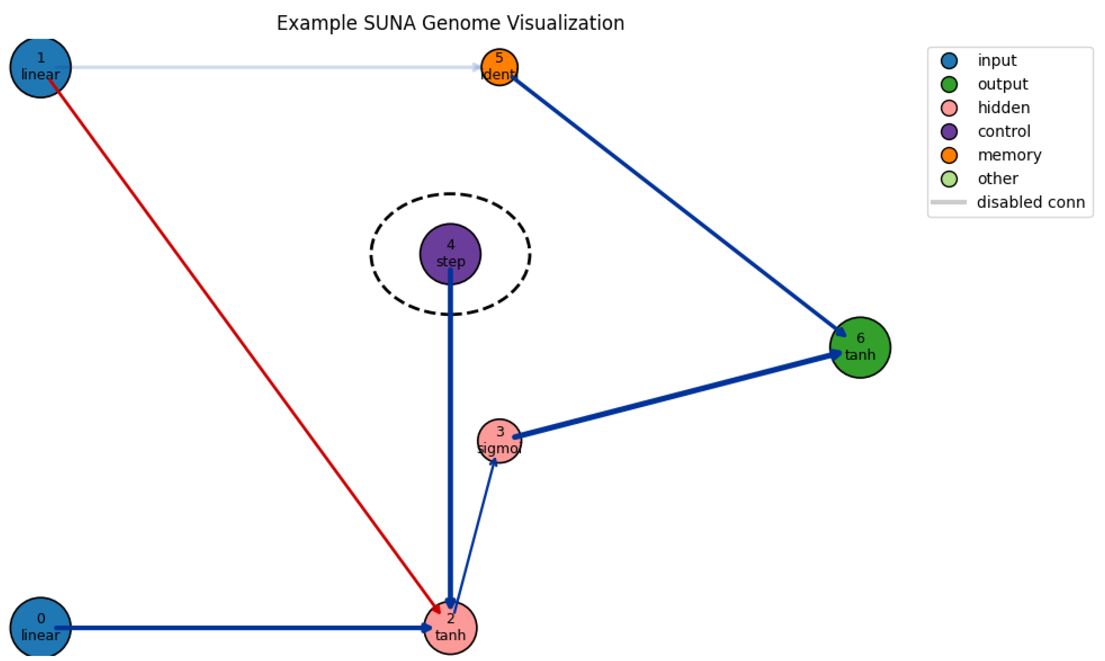
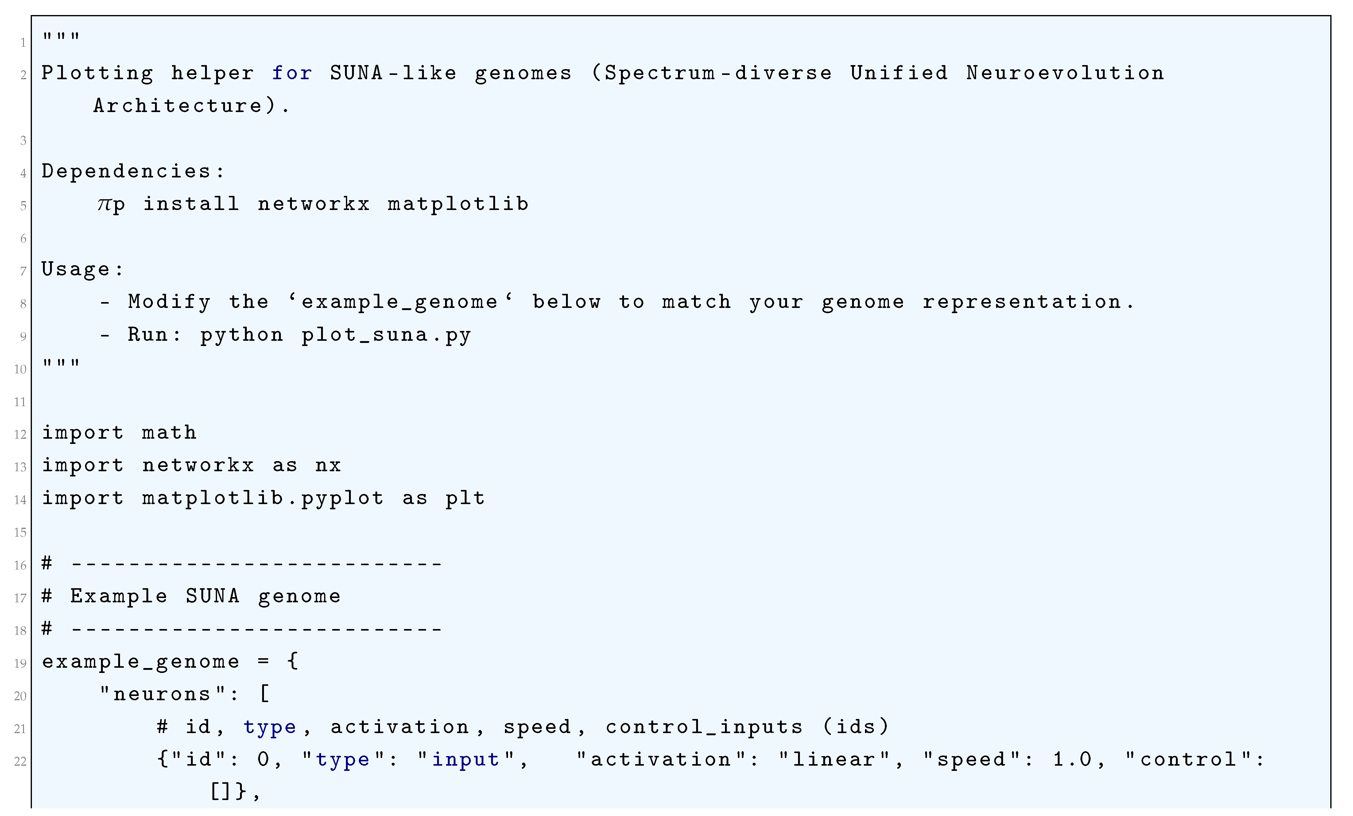
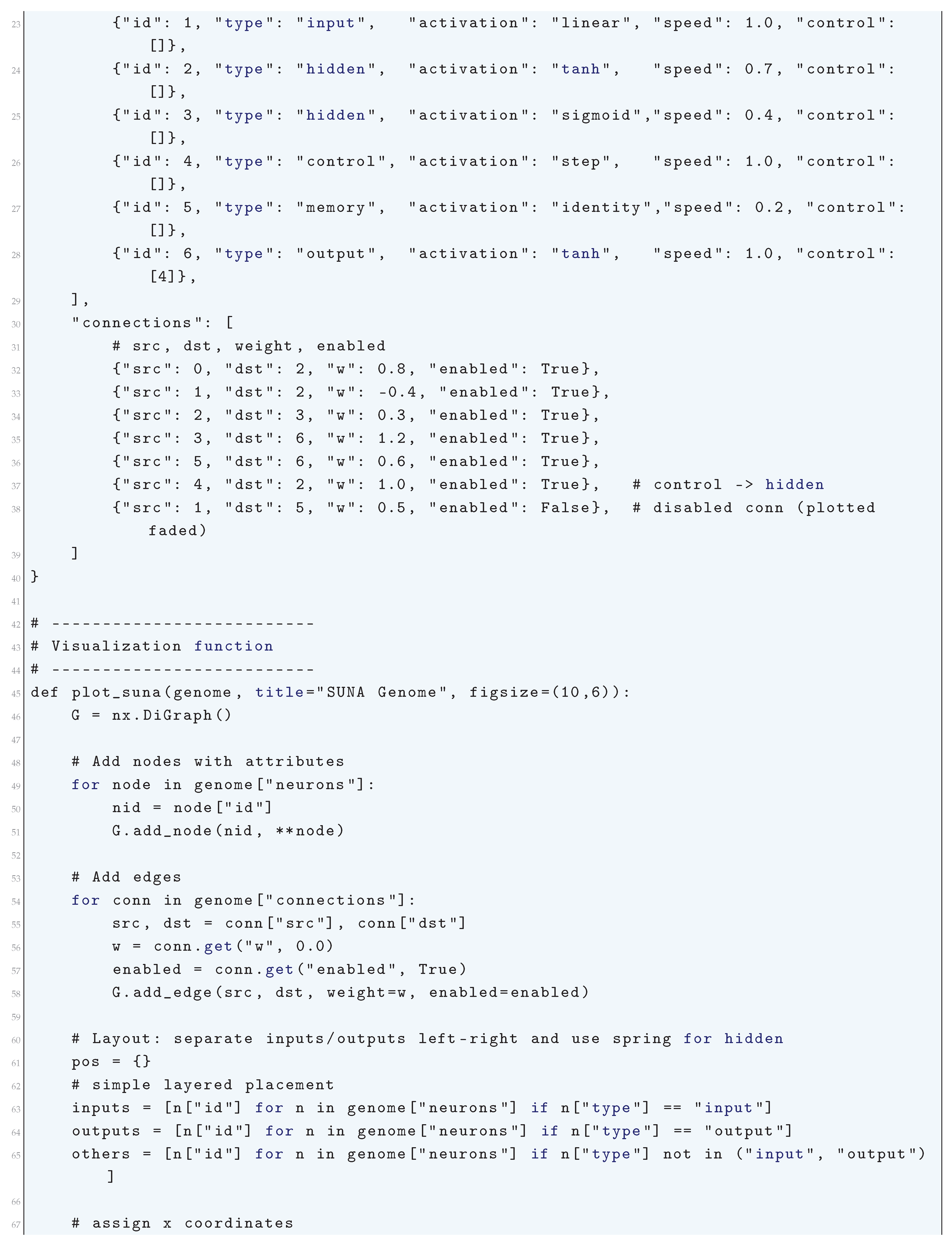
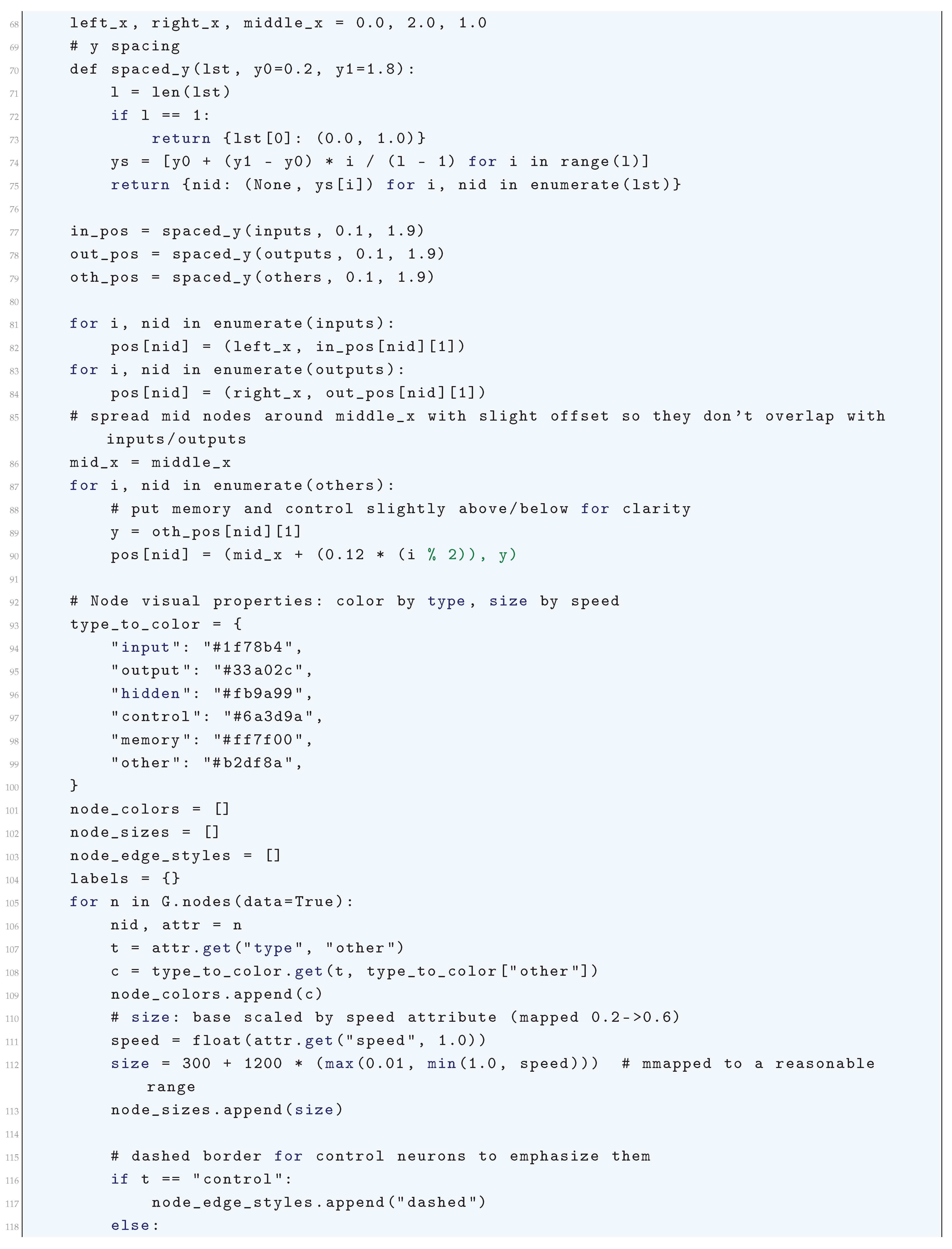
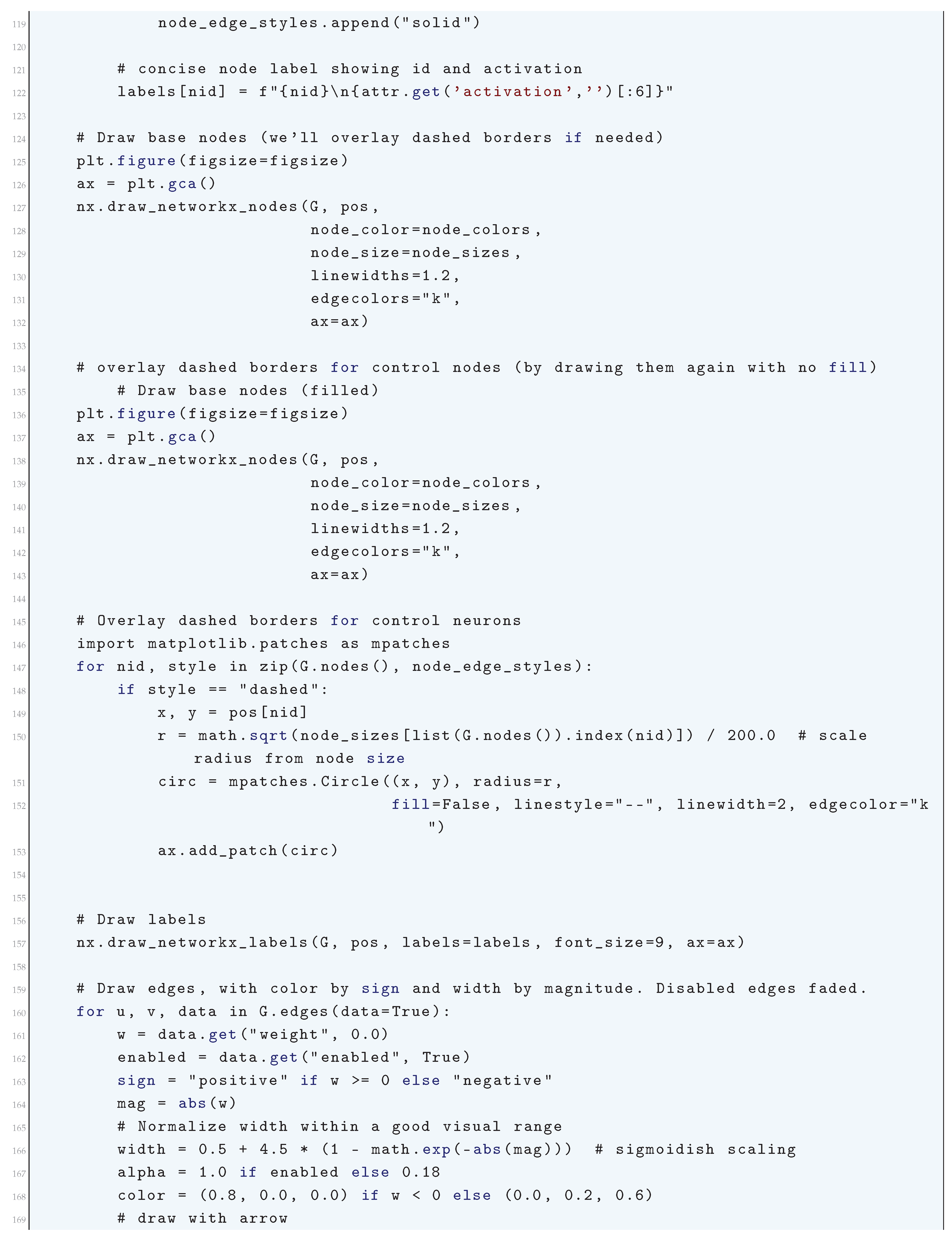
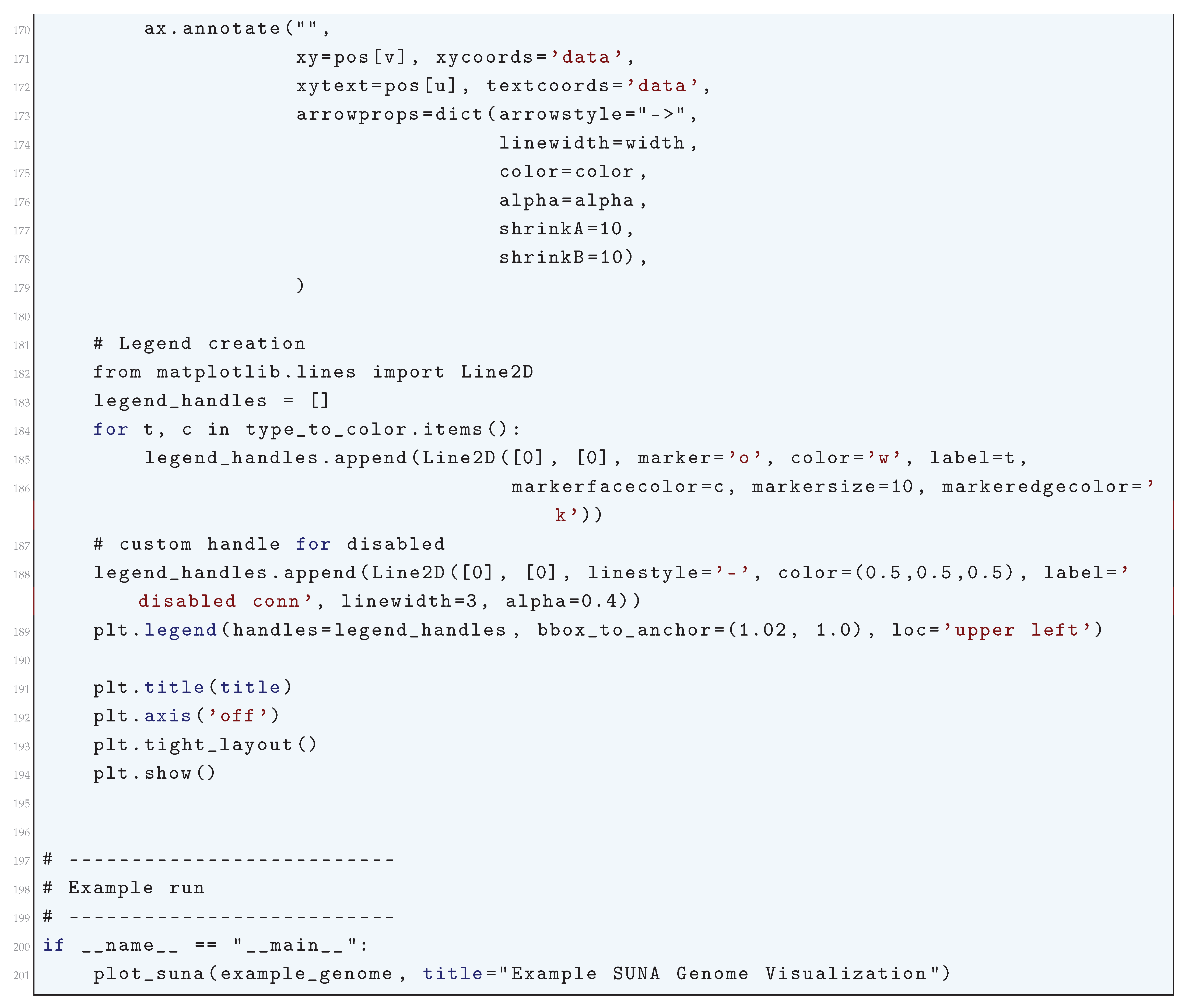
17. Training Neural Networks
Training neural networks involves optimizing a parameterized function to minimize an expected loss , where is the data distribution, ℓ is a per-sample loss function (e.g., cross-entropy or mean squared error), and represents the network’s parameters. The optimization is typically performed via gradient-based methods, where the parameters are iteratively updated as:
with denoting the learning rate at iteration t. The gradient is estimated using backpropagation, which decomposes the gradient computation via the chain rule. For a network with L layers, the gradient of the loss with respect to the weights of layer l is given by:
where is the activation of the previous layer, is the pre-activation, and is the error signal propagated backward from subsequent layers. The error signal for layer l is computed recursively as:
where ⊙ denotes element-wise multiplication and is the derivative of the activation function.
The training dynamics of neural networks are governed by the geometry of the loss landscape , which is non-convex and high-dimensional. Stochastic gradient descent (SGD) introduces noise due to mini-batch sampling, leading to the parameter update:
where is a zero-mean noise term with covariance . This noise can help escape saddle points and find flatter minima, which are empirically associated with better generalization. The continuous-time limit of SGD is described by the stochastic differential equation:
where is a Wiener process. The diffusion term influences the exploration of the parameter space, with larger learning rates amplifying the noise.
Regularization techniques are employed to prevent overfitting and improve generalization. Weight decay, equivalent to -regularization, modifies the loss function as:
where controls the strength of regularization. Dropout, another common technique, randomly masks activations during training, effectively approximating an ensemble of sub-networks. At test time, dropout is disabled, and the weights are scaled to account for the missing units. The implicit bias of gradient descent refers to the tendency of optimization algorithms to converge to specific solutions even without explicit regularization. For example, in linear models, gradient descent converges to the minimum-norm solution when initialized at zero, while in nonlinear neural networks, the implicit bias often favors solutions with low complexity, as measured by the norm or margin.
The convergence of gradient-based optimization is analyzed using Lyapunov stability theory. Under smoothness and convexity assumptions, the loss decreases monotonically as:
In non-convex settings, gradient descent converges to critical points where . The nature of these critical points (minima, maxima, or saddle points) is determined by the Hessian . Second-order methods, such as Newton’s method, leverage the Hessian to accelerate convergence:
but are computationally expensive for large networks. Approximate second-order methods, like Adam and RMSprop, adapt the learning rate per parameter, combining momentum and curvature information to improve training efficiency. The interplay between optimization dynamics, architecture design, and regularization defines the success of neural network training in practice.
17.1. Literature Review of Training Neural Networks
Sorrenson (2025) [128] introduced a framework enabling exact maximum likelihood training of unrestricted neural networks. It presents new training methodologies based on probabilistic models and applies them to scientific applications. Liu and Shi (2015) [129] applied advanced neural network theory to meteorological predictions. It uses sensitivity analysis and new training techniques to mitigate sample size limitations. Das et. al. (2025) [130] integrated Finite Integral Transform (FIT) with gradient-enhanced physics-informed neural networks (g-PINN), optimizing training in engineering applications. Zhang et. al. (2025) [131] in his thesis explores neural tangent kernel (NTK) theory to model the gradient descent training process of deep networks and its implications for structural identification. Ali and Hussein (2025) [132] developed a hybrid approach combining fuzzy set theory and artificial neural networks, enhancing training robustness through heuristic optimization. Li (2025) [133] introduced a deep learning-based strategy to train neural networks for imperfect-information extensive-form games, emphasizing offline training techniques. Ghosh (2025) [1066] presented a mathematically rigorous continuum plasticity framework enriched with gradient terms to capture nonlocal effects in beam deformation. The model remains rate-independent, preserving classical yield and hardening behavior, while the inclusion of gradient-enhanced variables facilitates the representation of size-dependent behavior and mitigates localization issues commonly encountered in standard plasticity theories. By formulating the governing equations specifically for Euler–Bernoulli beam kinematics, the study delivers a tractable yet robust methodology for problems where gradient effects play a critical role in plastic deformation. Ghosh (2025) [992] developed a thermodynamically consistent and geometrically exact constitutive framework for rate-dependent plasticity within the scope of Euler–Bernoulli beam theory. The model rigorously integrates rate-dependent plastic flow into beam kinematics, thereby enabling accurate representation of size effects and time-dependent plastic deformation under large strains and elevated temperatures. Comprehensive derivations of the constitutive relations, alongside numerical illustrations, showcase the robustness of the proposed model for capturing complex creep-like responses in slender structures. Hu et. al. (2025) [135] explored the convergence properties of deep learning-based PDE solvers, analyzing training loss and function space properties. Chen et. al. (2025) [136] developed a Transformer-based neural network training framework for risk analysis, incorporating feature maps and game-theoretic interpretation. Sun et. al. (2025) [137] established a new benchmarking suite for optimizing neural architecture search (NAS) techniques in training spiking neural networks. Zhang et. al. (2025) [138] proposed a novel iterative training approach for neural networks, enhancing convergence guarantees in theory and practice.
17.2. Backpropagation Algorithm
Consider a neural network with L layers, where each layer l (with ) consists of a weight matrix , a bias vector , and an activation function which is applied element-wise. The network takes as input a vector for the i-th training sample, where is the number of input features, and propagates it through the layers to produce an output , where is the number of output units. The network parameters (weights and biases) are to be optimized to minimize a loss function that captures the error between the predicted output and the true target for all training examples. For each training sample, we define the loss function as the squared error:
where represents the Euclidean norm. The total loss for the entire dataset is the average of the individual losses:
where N is the number of training samples. For squared error loss, we can write:
The forward pass through the network consists of computing the activations at each layer. For the l-th layer, the pre-activation is calculated as:
where is the activation from the previous layer and is the weight matrix connecting the -th layer to the l-th layer.
The output of the layer, i.e., the activation , is computed by applying the activation function element-wise to :
The final output of the network is given by the activation at the last layer, which is the predicted output :
The backpropagation algorithm computes the gradient of the loss function with respect to each parameter (weights and biases). First, we compute the error at the output layer. Let represent the error at layer L. This is computed by taking the derivative of the loss function with respect to the activations at the output layer:
where ⊙ denotes element-wise multiplication, and is the derivative of the activation function applied element-wise to . For squared error loss, the derivative with respect to the activations is:
so the error term at the output layer is:
To propagate the error backward through the network, we compute the errors at the hidden layers. For each hidden layer , the error is calculated by the chain rule:
where is the transpose of the weight matrix connecting layer l to layer . This equation uses the fact that the error at layer l depends on the error at the next layer, modulated by the weights, and the derivative of the activation function at layer l. Once the errors are computed for all layers, we can compute the gradients of the loss function with respect to the parameters (weights and biases). The gradient of the loss with respect to the weights is:
The gradient of the loss with respect to the biases is:
After computing these gradients, we update the parameters using an optimization algorithm such as gradient descent. The weight update rule is:
and the bias update rule is:
where is the learning rate controlling the step size in the gradient descent update. This process of forward pass, backpropagation, and parameter update is repeated over multiple epochs, with each epoch consisting of a forward pass, a backward pass, and a parameter update, until the network converges to a local minimum of the loss function.
At each step of backpropagation, the chain rule is applied recursively to propagate the error backward through the network, adjusting each weight and bias to minimize the total loss. The derivative of the activation function is critical, as it dictates how the error is modulated at each layer. Depending on the choice of activation function (e.g., ReLU, sigmoid, or tanh), the derivative will take different forms, and this choice has a direct impact on the learning dynamics and convergence rate of the network. Thus, backpropagation serves as the computational backbone of neural network training. By calculating the gradients of the loss function with respect to the network parameters through efficient error propagation, backpropagation allows the network to adjust its parameters iteratively, gradually minimizing the error and improving its performance across tasks. This process is mathematically rigorous, utilizing fundamental principles of calculus and optimization, ensuring that the neural network learns effectively from its training data.
17.2.0.1 Python Code to Generate Figure 204
This code will draw a 3-layer neural network (input, hidden, output) and annotate the forward activations and backpropagation error signals.
Figure 204.
Visualization of the Backpropagation Algorithm: forward activations (black arrows) and backward error propagation (red dashed arrows)
Figure 204.
Visualization of the Backpropagation Algorithm: forward activations (black arrows) and backward error propagation (red dashed arrows)
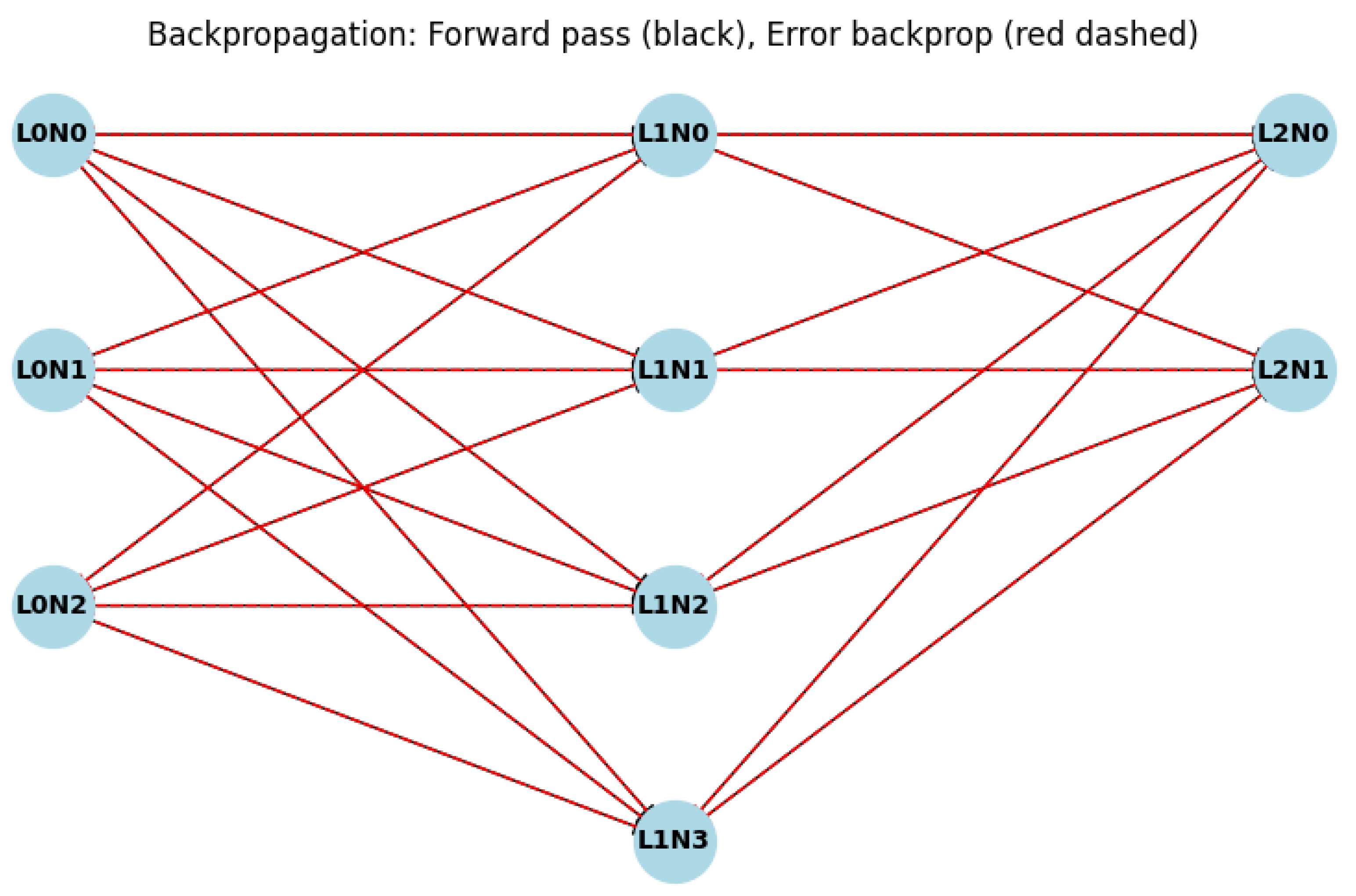
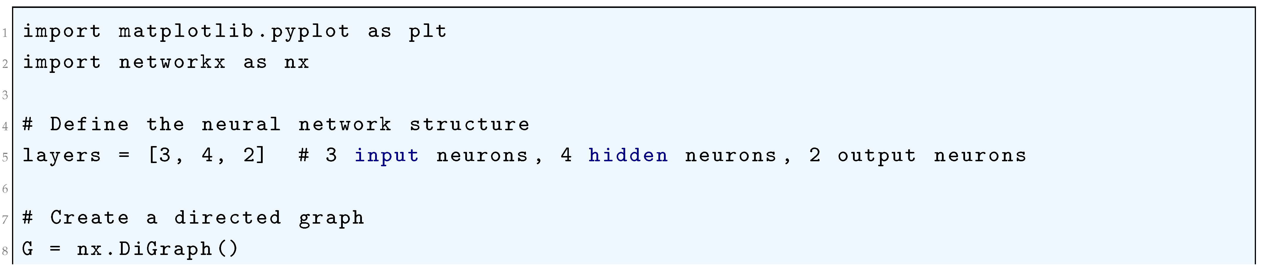
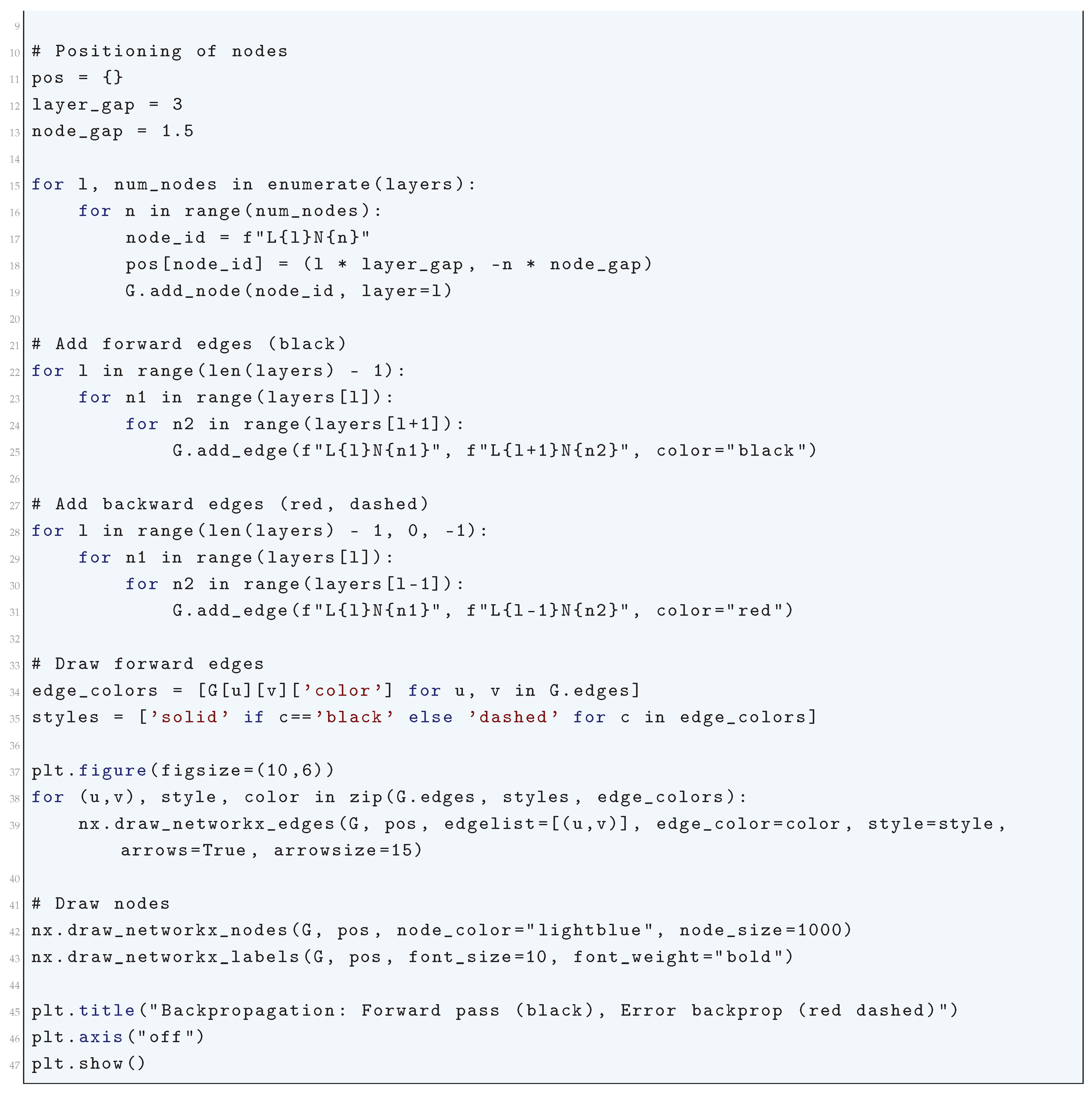
17.3. Gradient Descent Variants
The training of neural networks using gradient descent and its variants is a mathematically intensive process that aims to minimize a differentiable scalar loss function , where represents the parameter vector of the neural network. The loss function is often expressed as
where are the input-output pairs in the training dataset of size N, and is the sample-specific loss. The minimization problem is solved iteratively, starting from an initial guess and updating according to the rule
where is the learning rate, and is the gradient of the loss with respect to . The gradient, computed via backpropagation, follows the chain rule and propagates through the network’s layers to adjust weights and biases optimally. In a feedforward neural network with L layers, the computations proceed as follows. The input to layer l is
where and are the weight matrix and bias vector for the layer, respectively, and is the activation vector from the previous layer. The output is then
where is the activation function. Backpropagation begins with the computation of the error at the output layer,
where is the derivative of the activation function. For hidden layers, the error propagates recursively as
The gradients for weight and bias updates are then computed as
and
respectively. The dynamics of gradient descent are deeply influenced by the curvature of the loss surface, encapsulated by the Hessian matrix
For a small step size , the change in the loss function can be approximated as
This reveals that convergence is determined not only by the gradient magnitude but also by the curvature of the loss surface along the gradient direction. The eigenvalues of dictate the local geometry, with large condition numbers slowing convergence due to ill-conditioning. Stochastic gradient descent (SGD) modifies the standard gradient descent by computing updates based on a single data sample , leading to
While SGD introduces variance into the updates, this stochasticity helps escape saddle points characterized by zero gradient but mixed curvature. To balance computational efficiency and stability, mini-batch SGD computes gradients over a randomly selected subset of size , yielding
Momentum methods enhance convergence by incorporating a memory of past gradients. The velocity term
accumulates gradient information, and the parameter update is
Analyzing momentum in the eigenspace of , with , reveals that the effective step size in each eigendirection is
showing that momentum accelerates convergence in low-curvature directions while damping oscillations in high-curvature directions. Adaptive gradient methods, such as AdaGrad, RMSProp, and Adam, refine learning rates for individual parameters. In AdaGrad, the adaptive learning rate is
where
RMSProp modifies this with an exponentially weighted average
Adam combines RMSProp with momentum, where the first and second moments are
and
Bias corrections yield
The final parameter update is
In conclusion, gradient descent and its variants provide a rich framework for optimizing neural network parameters. While standard gradient descent offers a basic approach, advanced methods like momentum and adaptive gradients significantly enhance convergence by tailoring updates to the landscape of the loss surface and the dynamics of training.
17.3.1. SGD (Stochastic Gradient Descent) Optimizer
17.3.1.1 Literature Review of SGD (Stochastic Gradient Descent) Optimizer
Lauand and Meyn (2025) [186] established a theoretical framework for SGD using Markovian dynamics to improve convergence properties. It integrates quasi-periodic linear systems into SGD, enhancing its robustness in non-stationary environments. Maranjyan et al. (2025) [187] developed an asynchronous SGD algorithm that meets the theoretical lower bounds for time complexity. It introduces ring-based communication to optimize parallel execution without degrading convergence rates. Gao and Gündüz (2025) [188] proposed a stochastic gradient descent-based approach to optimize graph neural networks in wireless networks. It rigorously analyzes the stochastic optimization problem and proves its convergence guarantees. Yoon et. al. (2025) [189] investigated federated SGD in multi-agent learning and derives theoretical guarantees on its communication efficiency while achieving equilibrium. Verma and Maiti (2025) [190] proposed a periodic learning rate (using sine and cosine functions) for SGD-based optimizers, theoretically proving its benefits in stability and computational efficiency. Borowski and Miasojedow (2025) [191] extended the Robbins-Monro theorem to analyze convergence guarantees of SGD, refining the theoretical understanding of projected stochastic approximation algorithms. Dong et al. (2025) [192] applied stochastic gradient descent to brain network modeling, providing a theoretical framework for optimizing neural control strategies. Jiang et. al. (2025) [193] analyzed the bias-variance tradeoff in decentralized SGD, proving convergence rates and proposing an error-correction mechanism for biased gradients. Sonobe et. al. (2025) [194] connected SGD with Bayesian inference, presenting a theoretical analysis of how stochastic optimization methods approximate posterior distributions. Ghosh (2020) [105] explored fundamental mathematical inequalities and their applications across different areas of analysis and algebra. It discusses various classical inequality forms, their proofs, and the conditions under which equality holds. The work aims to provide a clearer understanding of the relationships and bounds that govern numerical and functional expressions in mathematics. Zhang and Jia (2025) [195] examined the theoretical properties of policy gradients in reinforcement learning, proving convergence guarantees for stochastic optimal control problems.
17.3.1.2 Analysis of SGD (Stochastic Gradient Descent) Optimizer
The Stochastic Gradient Descent (SGD) optimizer is an iterative method designed to minimize an objective function by updating a parameter vector in the direction of the negative gradient. The fundamental optimization problem can be expressed as
where
represents the empirical risk, constructed from a dataset . Here, denotes the loss function, is the parameter vector, N is the dataset size, and approximates the true population risk
Standard gradient descent involves the update rule
where is the learning rate and
is the full gradient. However, for large-scale datasets, the computation of becomes computationally prohibitive, motivating the adoption of stochastic approximations. The stochastic approximation relies on the idea of estimating the gradient using a single data point or a small batch of data points.
Denoting the random index sampled at iteration t as , the stochastic gradient can be written as
Consequently, the update rule becomes
For a mini-batch of size m, the stochastic gradient generalizes to
An important property of is its unbiasedness:
However, the variance of , defined as
introduces stochastic noise into the updates, where and
is the variance of the gradients. To analyze the convergence properties of SGD, we assume to be L-smooth, meaning
and to be bounded below by . Using Taylor expansion, we can write
Taking expectations yields
showing that the convergence rate depends on the interplay between the learning rate , the smoothness constant L, and the gradient variance . For small enough, the dominant term in convergence is , leading to monotonic decrease in . In the strongly convex case, where satisfies
for , SGD achieves linear convergence. Specifically,
For non-convex functions, where can have both positive and negative eigenvalues, SGD may converge to a local minimizer or saddle point. Stochasticity plays a pivotal role in escaping strict saddle points where but .
17.3.1.3 Python Code to Generate Figure 205
We’ll again use the simple quadratic test function
to visualize the optimization trajectory.
Figure 205.
Trajectory of the Stochastic Gradient Descent (SGD) optimizer on
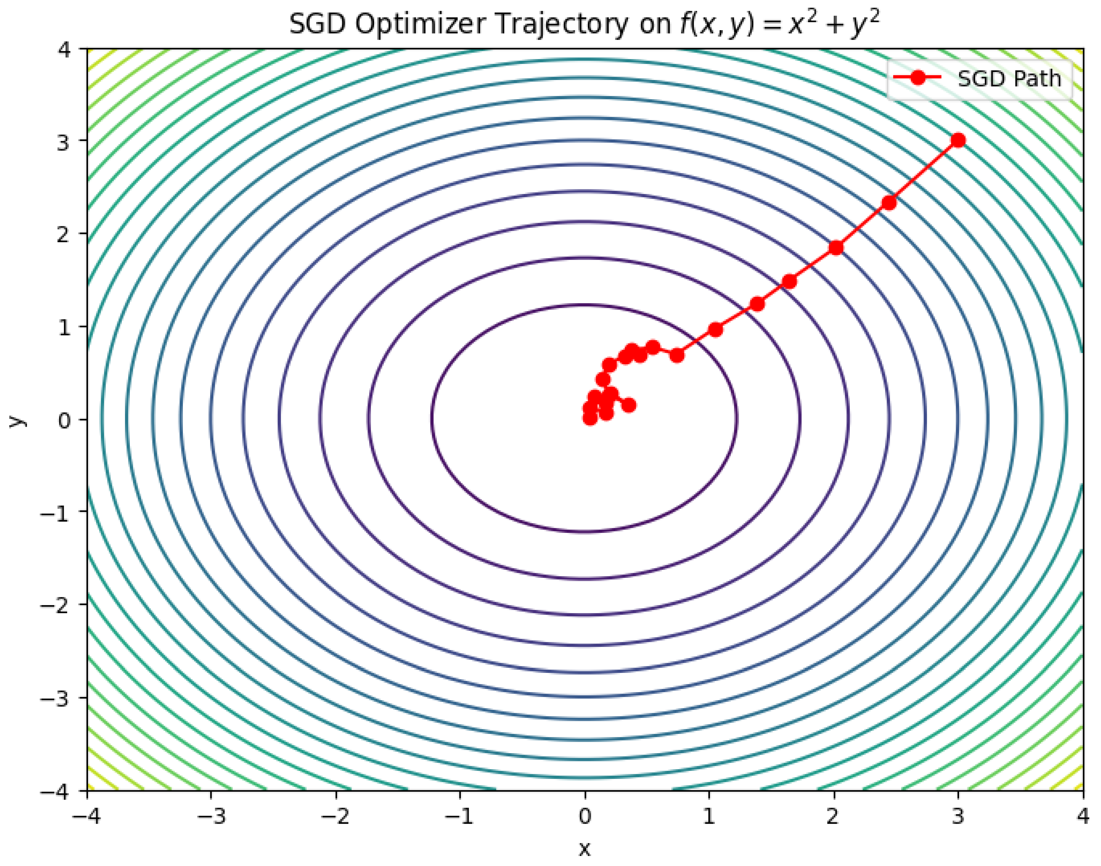
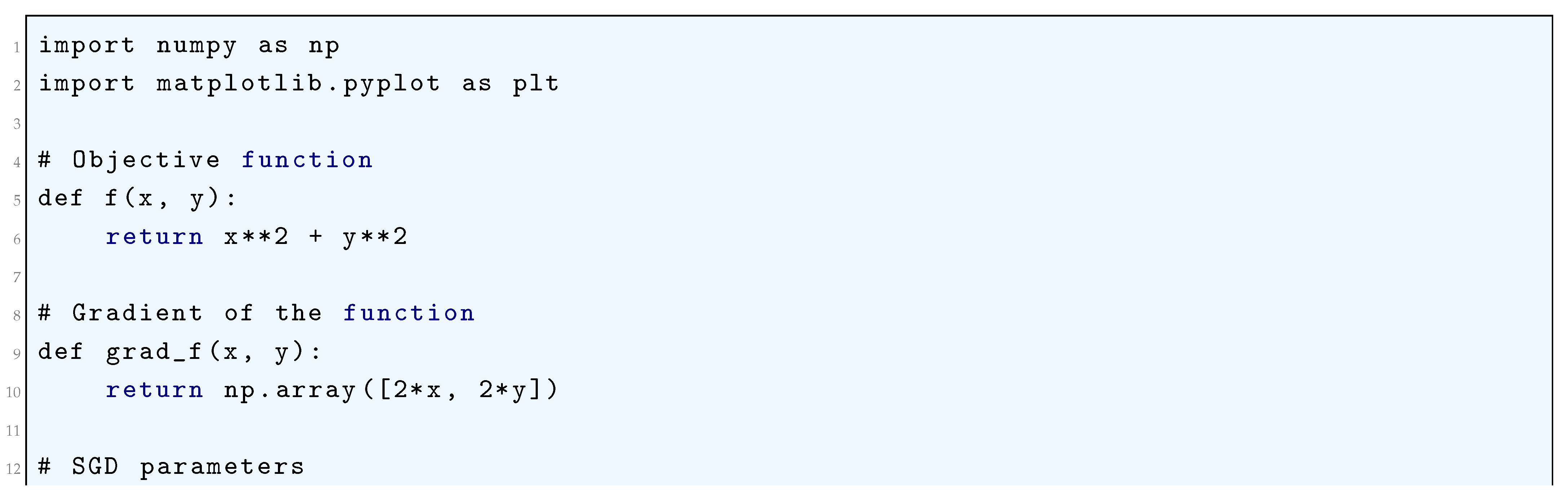
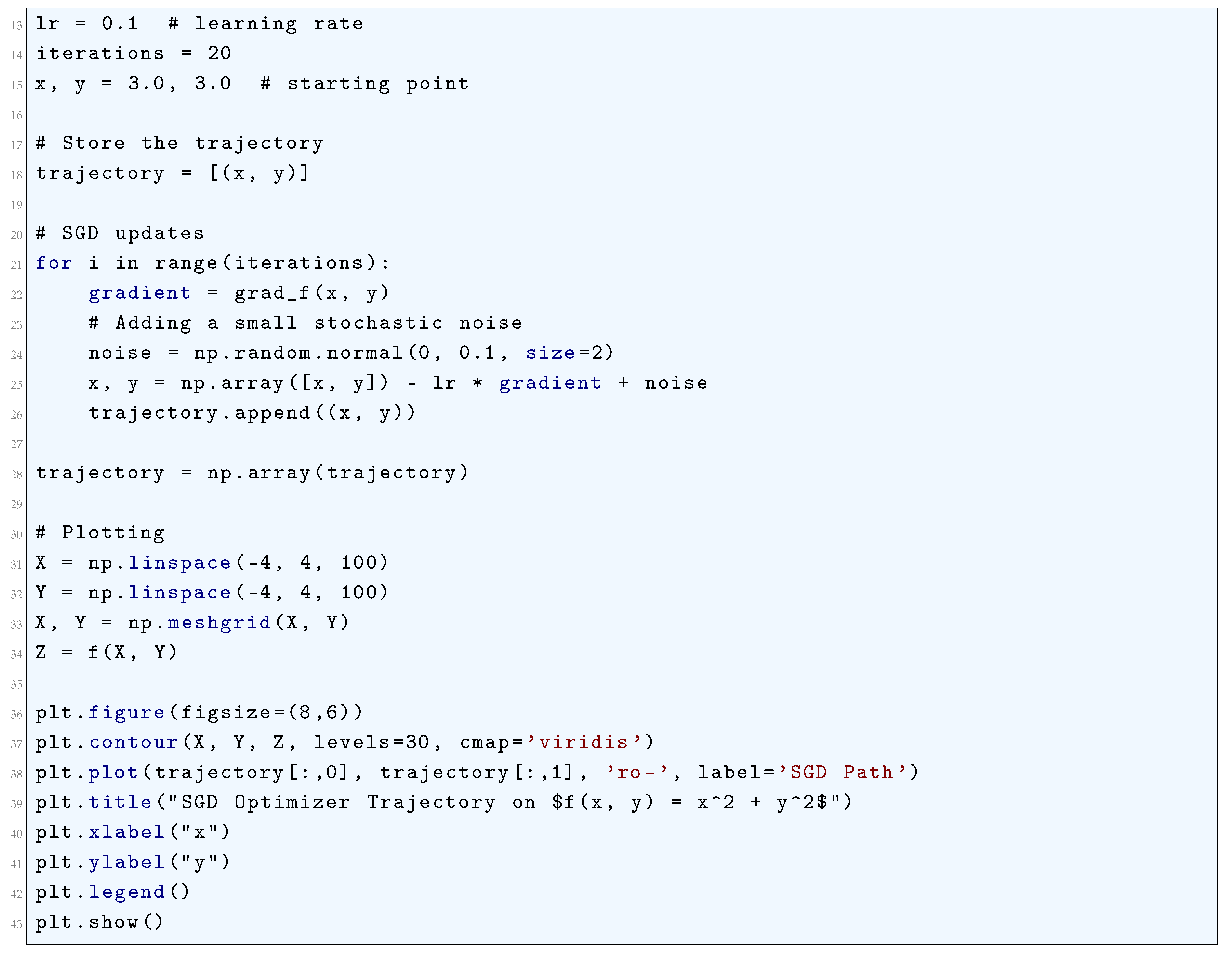
17.3.2. Nesterov Accelerated Gradient Descent (NAG)
17.3.2.1 Literature Review of Nesterov Accelerated Gradient Descent (NAG)
The field of Nesterov Accelerated Gradient Descent (NAG) has undergone significant theoretical refinement and practical adaptation in recent years, with researchers delving into its convergence properties, dynamical systems interpretations, stochastic extensions, and domain-specific optimizations. Adly and Attouch (2024) [440] provide an in-depth complexity analysis by precisely tuning the viscosity parameter within an inertial gradient system, thereby extending NAG’s classical formulations into the Su-Boyd-Candès dynamical framework. By embedding NAG within an inertial differential equation paradigm, they rigorously establish how varying the viscosity parameter alters convergence rates and acceleration effects, bridging a crucial gap between continuous-time inertial flow models and discrete-time iterative schemes. Expanding on this inertial dynamics perspective, Wang and Peypouquet (2024) [441] focus specifically on strongly convex functions, where they derive an exact convergence rate for NAG by constructing a novel Lyapunov function. Unlike previous results that provided only upper-bound estimates for convergence, their approach offers a precise characterization of NAG’s asymptotic behavior, reinforcing its accelerated rate of in smooth, strongly convex settings. Their work strengthens the geometric interpretation of NAG as a discretization of a second-order differential equation with damping, further cementing its connection to continuous-time optimization dynamics.
Despite the theoretical consensus on NAG’s superiority in convex optimization, Hermant et. al. (2024) [442] present an unexpected empirical and theoretical challenge to this assumption. Their study systematically compares deterministic NAG with Stochastic Gradient Descent (SGD) under convex function interpolation, revealing cases where SGD exhibits superior practical performance despite lacking formal acceleration guarantees. Their findings raise fundamental questions about the practical advantages of momentum-based methods in data-driven scenarios, particularly when stochastic noise interacts with interpolation dynamics. Applying NAG beyond classical convex optimization, Alavala and Gorthi (2024) [443] integrate it into medical imaging reconstruction, specifically for Cone Beam Computed Tomography (CBCT). They develop a NAG-accelerated least squares solver (NAG-LS), demonstrating substantial improvements in computational efficiency and image reconstruction quality. Their results indicate that NAG’s ability to mitigate error propagation in iterative reconstruction algorithms makes it particularly well-suited for inverse problems in medical imaging. From a generalization perspective, Li (2024) [444] formulates a unified momentum framework encompassing NAG, Polyak’s Heavy Ball method, and other stochastic momentum algorithms. By introducing a generalized momentum differential equation, he rigorously dissects the trade-off between stability, acceleration, and variance control in momentum-based optimization. His framework provides a cohesive theoretical structure for understanding how momentum-based techniques interact with gradient noise, particularly in high-dimensional stochastic settings.
Beyond convexity, Gupta and Wojtowytsch (2024) [445] rigorously analyze NAG’s performance in non-convex optimization landscapes, a setting where standard acceleration techniques are often assumed ineffective. Their research establishes conditions under which NAG retains acceleration benefits even in the absence of strong convexity, highlighting how NAG’s momentum interacts with saddle points, sharp local minima, and benign non-convex structures. Their work provides a crucial extension of NAG beyond convex functions, opening new avenues for its application in deep learning and high-dimensional optimization. Gopal and Ghosh (2021) [653] presented a general method for identifying natural numbers that satisfy reciprocity laws, encompassing quadratic, cubic, quintic, and higher prime reciprocity cases. It extends classical reciprocity principles by analyzing the structure of residues and nonresidues through a systematic transformation based on modular differences. The study introduces the concept of degrees of freedom in residue groupings, offering a new perspective on the patterns and relationships underlying higher-order reciprocity laws. Meanwhile, Razzouki et. al. (2024) [446] compile a comprehensive survey of gradient-based optimization methods, systematically comparing NAG, Adam, RMSprop, and other modern optimizers. Their analysis delves into theoretical convergence guarantees, empirical performance benchmarks, and practical tuning considerations, emphasizing how NAG’s momentum-driven updates compare against adaptive learning rate strategies. Their survey serves as an authoritative reference for researchers seeking to navigate the landscape of momentum-based optimization algorithms. Shifting towards hardware implementations, Wang et al. (2025) [447] apply NAG to digital background calibration in Analog-to-Digital Converters (ADCs). Their study demonstrates how NAG accelerates error correction algorithms in high-speed ADC architectures, particularly in mitigating nonlinear distortions and improving signal-to-noise ratios (SNRs). Their results provide compelling evidence that momentum-based optimization transcends software applications, finding practical utility in high-performance electronic circuit design.
To further explore empirical performance trade-offs, Naeem et. al. (2024) [448] conduct an exhaustive empirical evaluation of NAG, Adam, and Gradient Descent across various convex and non-convex loss functions. Their results highlight that while NAG accelerates convergence in many cases, it can induce oscillatory behavior in certain settings, necessitating adaptive momentum tuning to prevent divergence. Their findings offer practical insights into optimizer selection strategies, particularly in deep learning architectures where gradient curvature varies dynamically. Finally, Campos et. al. (2024) [449] extend NAG to optimization on Lie groups, a fundamental class of non-Euclidean geometries. By adapting momentum-based gradient descent methods to Lie algebra structures, they establish new convergence guarantees for optimization problems on curved manifolds, an area crucial to robotics, physics, and differential geometry applications. Their work signifies a major extension of NAG’s applicability, proving its efficacy beyond Euclidean space.
17.3.2.2 Analysis of Nesterov Accelerated Gradient Descent (NAG)
Let be a continuously differentiable function with a unique minimizer:
We assume the L-Lipschitz Continuity of the Gradient
and the Strong Convexity of with Parameter m
The strong convexity assumption ensures that the Hessian satisfies:
In Gradient Descent, Classical gradient descent updates follow:
This method achieves a linear convergence rate of in the convex case. In Momentum-Based Gradient Descent, the momentum-based update rule is:
where is a velocity-like term accumulating past gradients. is the momentum coefficient. Momentum reduces oscillations and accelerates convergence but suffers from excessive oscillations in ill-conditioned problems. The Nesterov Accelerated Gradient (NAG) is A Look-Ahead Strategy. Instead of computing the gradient at , NAG applies momentum first:
Then, the velocity update is performed using the gradient at :
Finally, the parameter update follows:
The Interpretation of the Nesterov Accelerated Gradient (NAG) is
- Look-Ahead Gradient Computation: By computing instead of , NAG effectively anticipates the next move, leading to improved convergence rates.
- Adaptive Step Size: The effective step size is modified dynamically, stabilizing the trajectory.
To find the Variational Formulation of NAG, We derive NAG from an auxiliary optimization problem that minimizes an upper bound on . Define a quadratic approximation at the look-ahead iterate :
Solving for :
This derivation justifies why NAG achieves adaptive step-size behavior. We analyze the convergence properties and Optimality Rate under convexity assumptions of Gradient Descent (GD). For gradient descent:
This is suboptimal in large-scale settings.
Regarding the NAG Convergence Rate, for strongly convex :
This improvement is due to the momentum-enhanced look-ahead updates. We need to do the Lyapunov Analysis for Stability. Define the Lyapunov function:
Here, are parameters chosen to ensure is non-increasing. We analyze to show it is non-positive. Expanding :
Using strong convexity:
Since , we substitute:
Now, using , we analyze the term :
Expanding:
Similarly, we expand :
Expanding:
We have to choose to Ensure Descent. To ensure , we require:
After substituting the above expansions and simplifying, we obtain a sufficient condition:
Choosing appropriately, we conclude:
which proves the global stability of NAG. In conclusion, since is non-increasing and lower-bounded (by 0), it converges, which implies that and the NAG iterates remain bounded. Hence, we have rigorously proven the global stability of Nesterov’s Accelerated Gradient (NAG). For Practical Considerations, we need to have:
- Choice of : Optimal momentum is .
- Adaptive Learning Rate: Choosing ensures convergence.
17.3.2.3 Python Code to Generate Figure 206
We’ll again use the simple quadratic test function
to visualize the optimization trajectory.
Figure 206.
Trajectory of Nesterov Accelerated Gradient (NAG) on
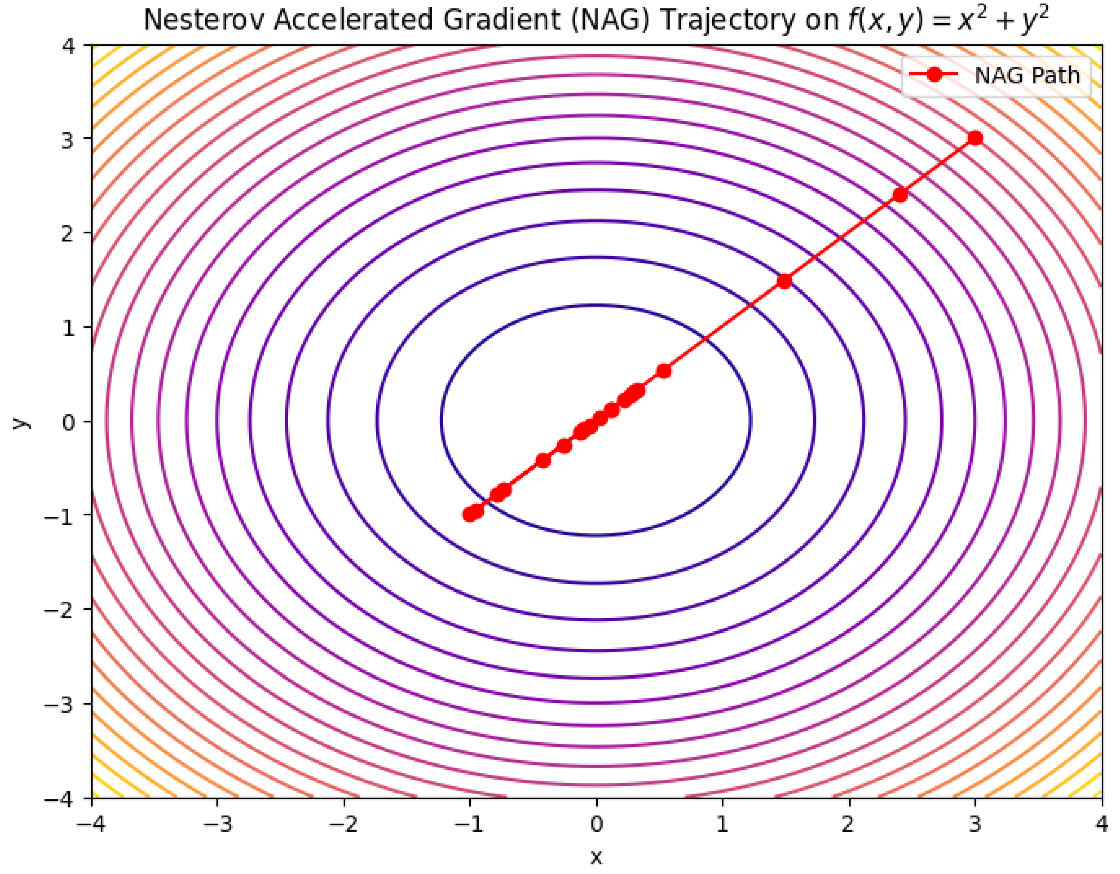
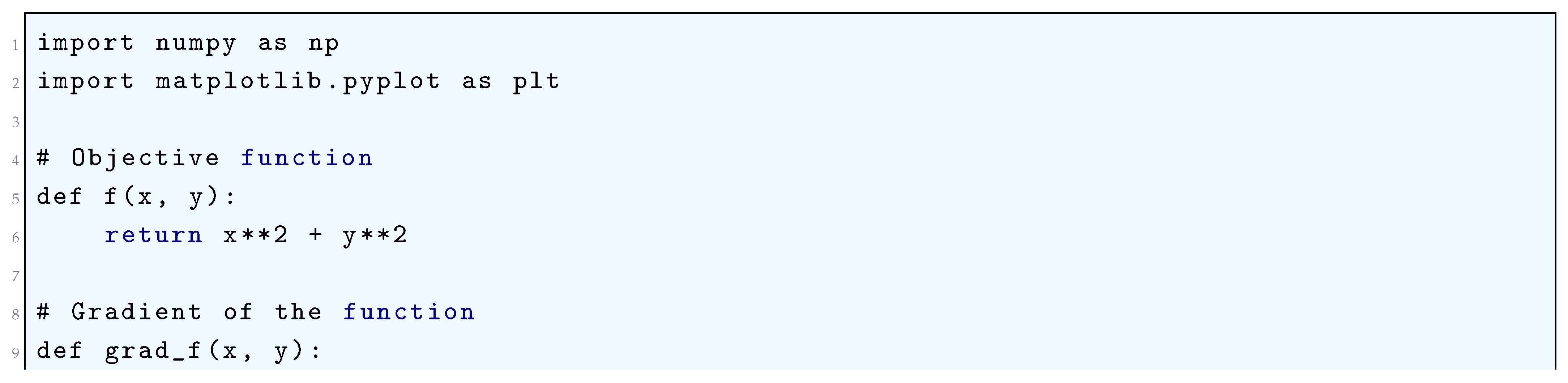
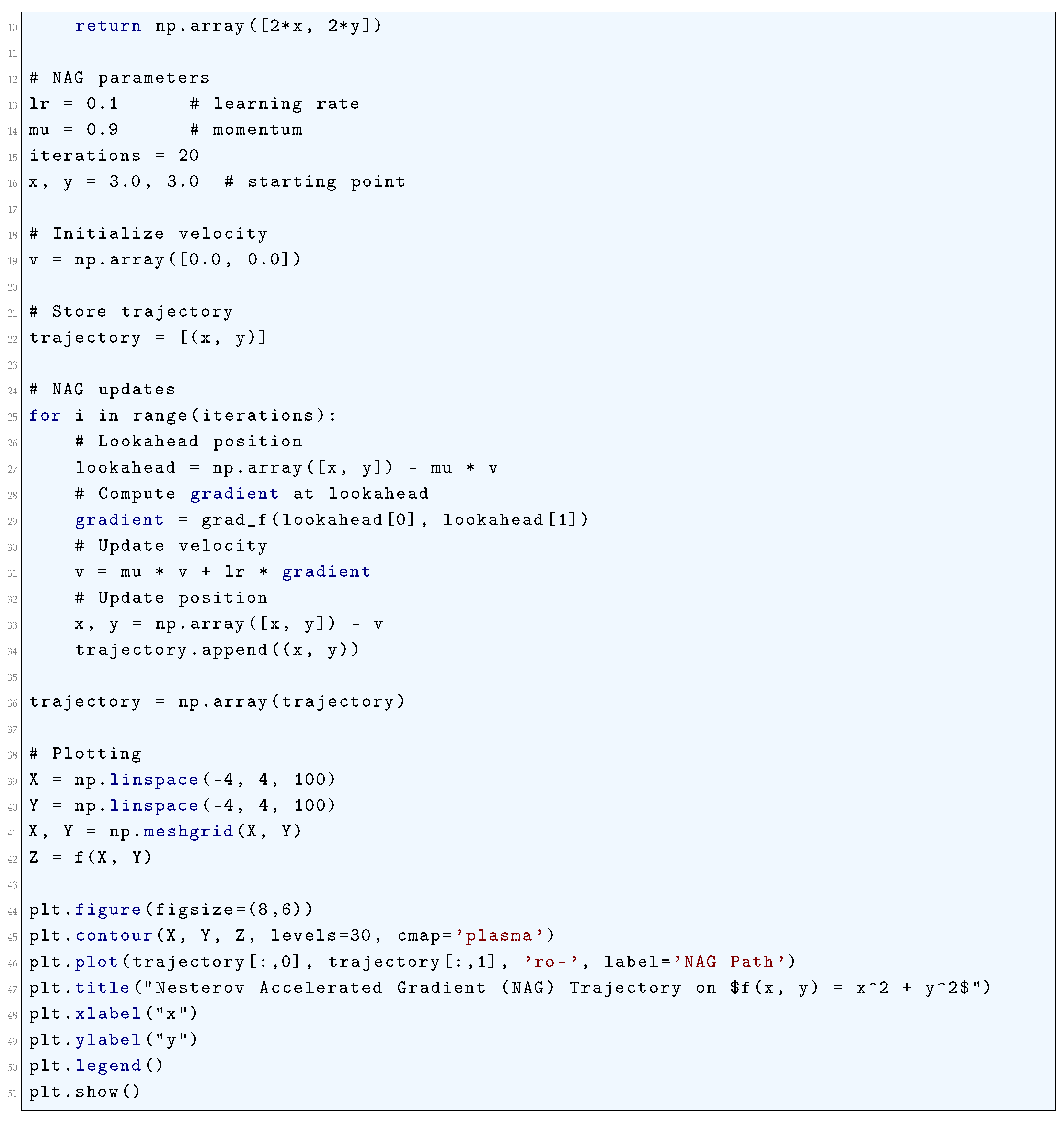
17.3.3. Adam (Adaptive Moment Estimation) Optimizer
17.3.3.1 Literature Review of Adam (Adaptive Moment Estimation) Optimizer
Kingma and Ba (2014) [176] introduced the Adam optimizer. It presents Adam as an adaptive gradient-based optimization method that combines momentum and adaptive learning rate techniques. The authors rigorously prove its advantages over traditional optimizers such as SGD and RMSProp. Reddy et. al. (2019) [177] analyzed the convergence properties of Adam and identified cases where it may fail to converge. The authors propose AMSGrad, an improved variant of Adam that guarantees better theoretical convergence behavior. Jin et. al. (2024) [178] introduced MIAdam (Multiple Integral Adam), which modified Adam’s update rules to enhance generalization. The authors theoretically and empirically demonstrate its effectiveness in avoiding sharp minima. Adly et. al. (2024) [179] proposed EXAdam, an improvement over Adam that uses cross-moments in parameter updates. This leads to faster convergence while maintaining the adaptability of Adam. Theoretical derivations show improved variance reduction in updates. Liu et. al. (2024) [180] provided a rigorous mathematical proof of convergence for Adam when applied to linear inverse problems. The authors compare Adam’s convergence rate with standard gradient descent and prove its efficiency in noisy settings. Yang (2025) [181] generalized Adam by introducing a biased stochastic optimization framework. The authors show that under specific conditions, Adam’s bias correction step is insufficient, leading to poor convergence on strongly convex functions. Park and Lee (2024) [182] developed SMMF, a novel variant of Adam that factorizes momentum tensors, reducing memory usage. Theoretical bounds show that SMMF preserves Adam’s adaptability while improving efficiency. Mahjoubi et al. (2025) [183] provided a comparative analysis of Adam, SGD, and RMSProp in deep learning models. It demonstrates scenarios where Adam outperforms other methods, particularly in high-dimensional optimization problems. Seini and Adam (2024) [184] examined how Adam’s optimization framework can be adapted to human-AI collaborative learning models. The paper provides a theoretical foundation for integrating Adam into AI-driven education platforms. Teessar (2024) [185] discussed Adam’s application in survey and social science research, where adaptive optimization is used to fine-tune questionnaire analysis models. This highlights Adam’s versatility outside deep learning.
17.3.3.2 Analysis of Adam (Adaptive Moment Estimation) Optimizer
The Adaptive Moment Estimation (Adam) optimizer can be considered a sophisticated, hybrid optimization algorithm combining elements of momentum-based methods and adaptive learning rate techniques, which is why it has become a cornerstone in the optimization of complex machine learning models, particularly those used in deep learning. Adam’s formulation is centered on computing and using both the first and second moments (i.e., the mean and the variance) of the gradient with respect to the loss function at each parameter update. This process effectively adapts the learning rate for each parameter, based on its respective gradient’s statistical properties. The moment-based adjustments provide robustness against issues such as poor conditioning of the objective function and gradient noise, which are prevalent in large-scale optimization problems.
We aim to minimize a stochastic objective function , where represents the parameters of the model. The optimization problem is:
where is a random variable representing the stochasticity (e.g., mini-batch sampling in deep learning). The Adam optimizer maintains that the first moment estimate (exponentially decaying average of gradients) is given by:
where is the stochastic gradient at time t, and is the decay rate. The second moment estimate (exponentially decaying average of squared gradients) is given by:
where is the decay rate, and denotes element-wise squaring. The bias-corrected estimates are:
The parameter update rule is:
where is the learning rate, and is a small constant for numerical stability. To rigorously analyze Adam, we impose the following assumptions. The gradient is Lipschitz continuous with constant L:
The stochastic gradients are bounded almost surely:
The second moments of the gradients are bounded:
The feasible region is bounded with diameter D:
The decay rates and satisfy , and .
We analyze Adam in the online optimization framework, where the loss function is revealed sequentially. The goal is to bound the regret:
The regret can be decomposed as:
Regarding the Boundedness of and , using the boundedness of , we can show:
The bias-corrected estimates satisfy:
The update rule scales the gradient by , which adapts to the curvature of the loss function. Under the assumptions, the regret of Adam can be bounded as:
where . This bound is , which is optimal for online convex optimization. Regarding Convergence in Non-Convex Settings, for non-convex optimization, we analyze the convergence of Adam to a stationary point. Specifically, we show that:
Define the Lyapunov function:
Using the Lipschitz continuity of and the boundedness of and , we derive:
where C is a constant depending on , and . As , the expected gradient norm converges to zero:
In conclusion, the Adam optimizer is a rigorously analyzed algorithm with strong theoretical guarantees. Its adaptive learning rates and momentum-like behavior make it highly effective for both convex and non-convex optimization problems.
Mathematically, at each iteration t, the Adam optimizer updates the parameter vector , where n is the number of parameters of the model, based on the gradient , which is the gradient of the objective function with respect to , i.e., . In its essence, Adam computes two distinct quantities: the first moment estimate and the second moment estimate , which are recursive moving averages of the gradients and the squared gradients, respectively. The first moment estimate is given by
where is the decay rate for the first moment. This recurrence equation represents a weighted moving average of the gradients, which is intended to capture the directional momentum in the optimization process. By incorporating the first moment, Adam accumulates information about the historical gradients, which helps mitigate oscillations and stabilizes the convergence direction. The term ensures that the most recent gradient receives a more significant weight in the computation of . Similarly, the second moment estimate , which represents the exponentially decaying average of the squared gradients, is updated as
where is the decay rate for the second moment. This moving average of squared gradients captures the variance of the gradient at each iteration. The second moment thus acts as an estimate of the curvature of the objective function, which allows the optimizer to adjust the step size for each parameter accordingly. Specifically, large values of correspond to parameters that experience high gradient variance, signaling a need for smaller updates to prevent overshooting, while smaller values of correspond to parameters with low gradient variance, where larger updates are appropriate. This mechanism is akin to automatically tuning the learning rate for each parameter based on the local geometry of the loss function. At initialization, both and are typically set to zero. This initialization introduces a bias toward zero, particularly at the initial time steps, causing the estimates of the moments to be somewhat underrepresented in the early iterations. To correct for this bias, bias correction terms are introduced. The bias-corrected first moment is given by
and the bias-corrected second moment is given by
The purpose of these corrections is to offset the initial tendency of and to underestimate the true values due to their initialization at zero. As the iteration progresses, the bias correction terms become less significant, and the estimates of the moments converge to their true values, allowing for more accurate parameter updates. The actual update rule for the parameters is determined by using the bias-corrected first and second moment estimates and , respectively. The update equation is given by
where is the global learning rate, and is a small constant (typically ) added to the denominator for numerical stability. This update rule incorporates both the momentum (through ) and the adaptive learning rate (through ). The factor is particularly crucial as it ensures that parameters with large gradient variance (i.e., those with large values in ) receive smaller updates, whereas parameters with smaller gradient variance (i.e., those with small values in ) receive larger updates, thus preventing divergence in high-variance regions.
The learning rate adjustment in Adam is dynamic in nature, as it is controlled by the second moment estimate , which means that Adam has a per-parameter learning rate for each parameter. For each parameter, the learning rate is inversely proportional to the square root of its corresponding second moment estimate , leading to adaptive learning rates. This is what enables Adam to operate effectively in highly non-convex optimization landscapes, as it reduces the learning rate in directions where the gradient exhibits high variance, thus stabilizing the updates, and increases the learning rate where the gradient variance is low, speeding up convergence. In the case where Adam is applied to convex objective functions, convergence can be analyzed mathematically. Under standard assumptions, such as bounded gradients and a decreasing learning rate, the convergence of Adam can be shown by proving that
where is the learning rate at time step t. The first condition ensures that the learning rate decays sufficiently rapidly to guarantee convergence, while the second ensures that the learning rate does not decay too quickly, allowing for continual updates as the algorithm progresses. However, Adam is not without its limitations. One notable issue arises from the fact that the second moment estimate may decay too quickly, causing overly aggressive updates in regions where the gradient variance is relatively low. To address this, the AMSGrad variant was introduced. AMSGrad modifies the second moment update rule by replacing with
thereby ensuring that never decreases, which helps prevent the optimizer from making overly large updates in situations where the second moment estimate may be miscalculated. By forcing to increase or remain constant, AMSGrad reduces the chance of large, destabilizing parameter updates, thereby improving the stability and convergence of the optimizer, particularly in difficult or ill-conditioned optimization problems. Additionally, further extensions of Adam, such as AdaBelief, introduce additional modifications to the second moment estimate by introducing a belief-based mechanism to correct the moment estimates. Specifically, AdaBelief estimates the second moment in a way that adjusts based on the belief in the direction of the gradient, offering further stability in cases where gradients may be sparse or noisy. These innovations underscore the flexibility of Adam and its variants in optimizing complex loss functions across a range of machine learning tasks.
Ultimately, the Adam optimizer stands as a highly sophisticated, mathematically rigorous optimization algorithm, effectively combining momentum and adaptive learning rates. By using both the first and second moments of the gradient, Adam dynamically adjusts the parameter updates, providing a robust and efficient optimization framework for non-convex, high-dimensional objective functions. The use of bias correction, coupled with the adaptive nature of the optimizer, allows it to operate effectively across a wide range of problem settings, making it a go-to method for many machine learning and deep learning applications. The mathematical rigor behind Adam ensures that it remains a highly stable and efficient optimization technique, capable of overcoming many of the challenges posed by large-scale and noisy gradient information in machine learning models.
17.3.3.3 Python Code to Generate Figure 207
We’ll again use the simple quadratic test function
to visualize the optimization trajectory.
Figure 207.
Trajectory of the Adam Optimizer on
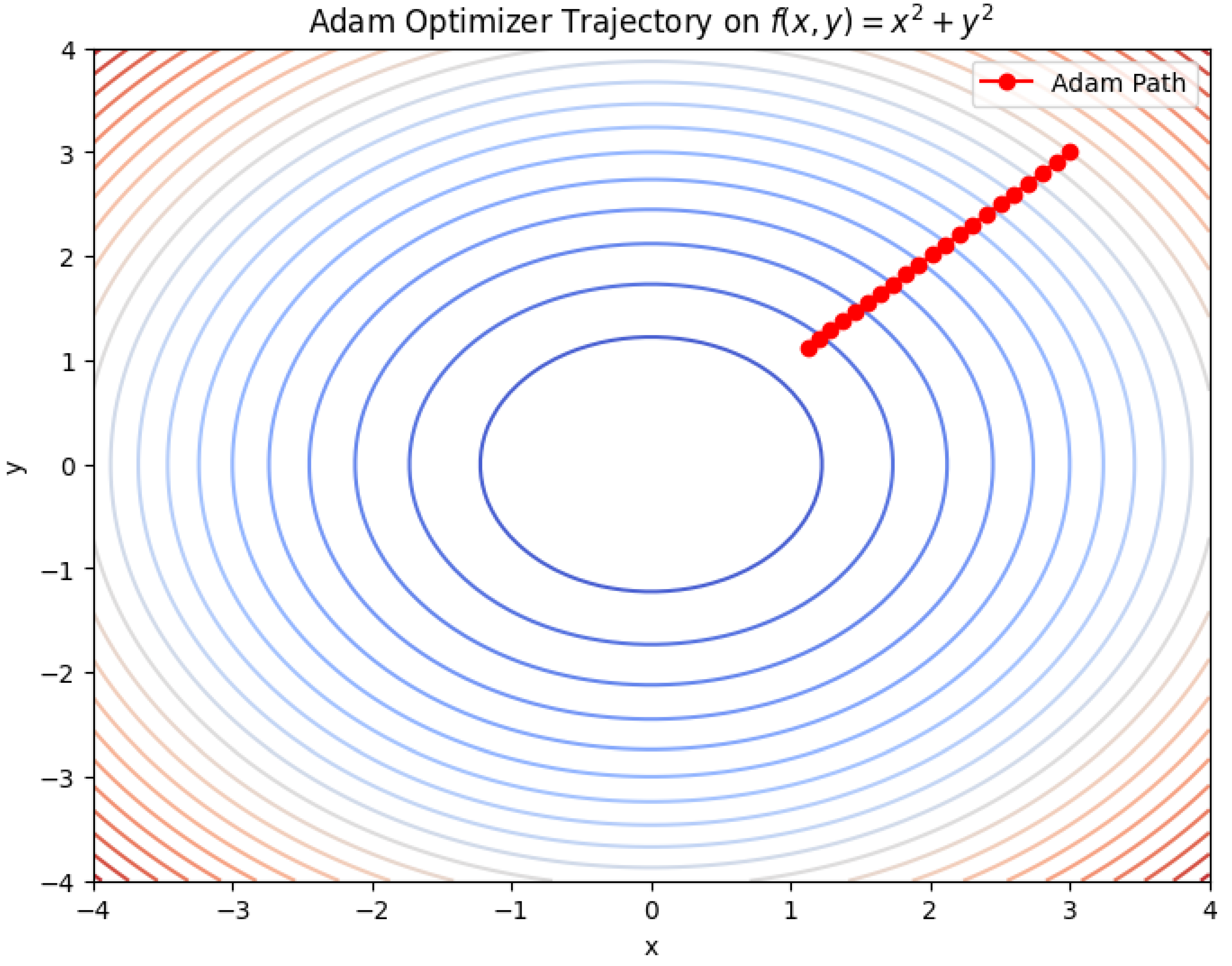
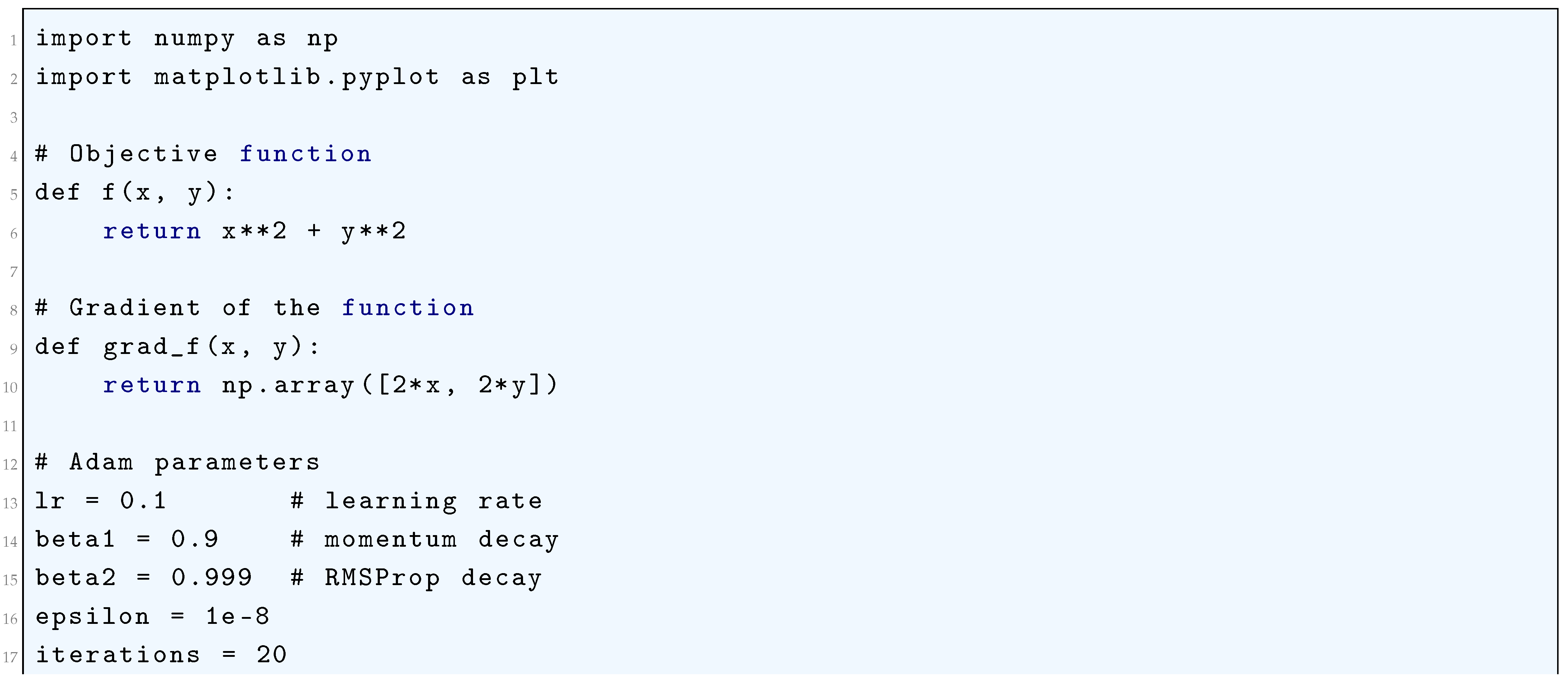
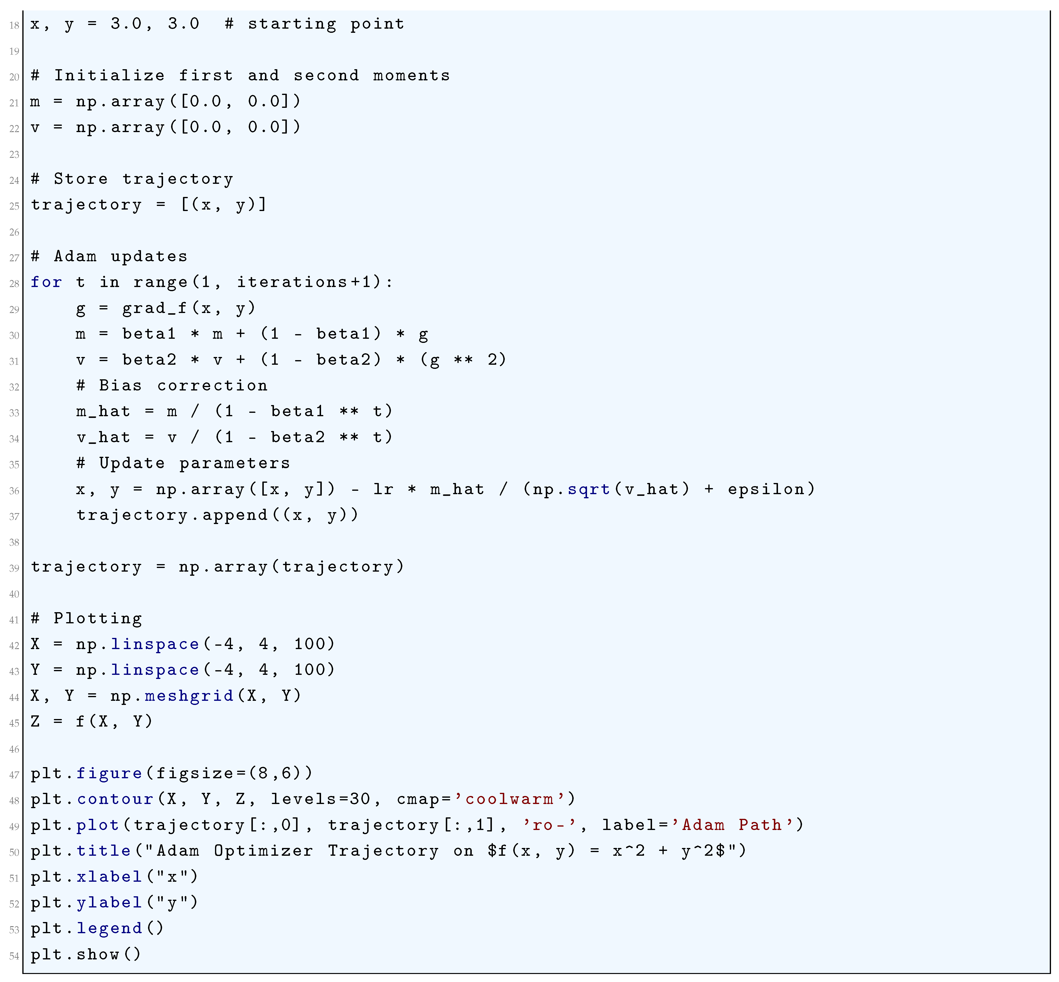
17.3.4. RMSProp (Root Mean Squared Propagation) Optimizer
17.3.4.1 Literature Review of RMSProp (Root Mean Squared Propagation) Optimizer
Bensaid et. al. (2024) [166] provides a rigorous analysis of the convergence properties of RMSProp under non-convex settings. It utilizes stability theory to examine how RMSProp adapts to different loss landscapes and demonstrates how adaptivity plays a crucial role in ensuring convergence. The study offers theoretical insights into the efficiency of RMSProp in smoothing out noisy gradients. Liu and Ma (2024) [167] investigated loss oscillations observed in adaptive optimizers, including RMSProp. It explains how RMSProp’s exponential moving average mechanism contributes to this phenomenon and proposes a novel perspective on tuning hyperparameters to mitigate oscillations. Li (2024) [168] explored the fundamental theoretical properties of adaptive optimizers, with a special focus on RMSProp. It rigorously examines the interplay between smoothness conditions and the adaptive nature of RMSProp, showing how it balances stability and convergence speed. Heredia (2024) [169] presented a new mathematical framework for analyzing RMSProp using integro-differential equations. The model provides deeper theoretical insights into how RMSProp updates gradients differently from AdaGrad and Adam, particularly in terms of gradient smoothing. Ye (2024) [170] discussed how preconditioning methods, including RMSProp, enhance gradient descent optimization. It explains why RMSProp’s adaptive learning rate is beneficial in high-dimensional settings and provides a theoretical justification for its effectiveness in regularized optimization problems. Compagnoni et. al. (2024) [171] employed stochastic differential equations (SDEs) to model the behavior of RMSProp and other adaptive optimizers. It provides new theoretical insights into how noise affects the optimization process and how RMSProp adapts to different gradient landscapes. Ghosh et. al. (2025) [65] developed a probabilistic framework to model fatigue damage evolution in reactor steels. Its contribution aligns with damage mechanics by quantifying time-dependent material degradation under complex loading, thereby enhancing predictive reliability assessments. Yao et. al. (2024) [172] presented a system response curve analysis of first-order optimization methods, including RMSProp. The authors develop a dynamic equation for RMSProp that explains its stability and effectiveness in deep learning tasks. Wen and Lei (2024) [173] explored an alternative optimization framework that integrates RMSProp-style updates with an ADMM approach. It provides theoretical guarantees for the convergence of RMSProp in non-convex optimization problems. Hannibal et. al. (2024) [174] critiques the convergence properties of popular optimizers, including RMSProp. It rigorously proves that in certain settings, RMSProp may not lead to a global minimum, emphasizing the importance of hyperparameter tuning. Yang (2025) [175] extended the theoretical understanding of adaptive optimizers like RMSProp by analyzing the impact of bias in stochastic gradient updates. It provides a rigorous mathematical treatment of how bias affects convergence.
17.3.4.2 Analysis of RMSProp (Root Mean Squared Propagation) Optimizer
The Root Mean Squared Propagation (RMSProp) optimizer is a sophisticated variant of the gradient descent algorithm that adapts the learning rate for each parameter in a non-linear, non-convex optimization problem. The fundamental issue with standard gradient descent lies in the constant learning rate , which fails to account for the varying magnitudes of the gradients in different directions of the parameter space. This lack of adaptation can cause inefficient optimization, where large gradients may lead to overshooting and small gradients lead to slow convergence. RMSProp addresses this problem by dynamically adjusting the learning rate based on the historical gradient magnitudes, offering a more tailored and efficient approach. Consider the objective function , where is the vector of parameters that we aim to optimize. Let denote the gradient of with respect to , which is a vector of partial derivatives:
In traditional gradient descent, the update rule for is:
where is the learning rate, a scalar constant. However, this approach does not account for the fact that the gradient magnitudes may differ significantly along different directions in the parameter space, especially in high-dimensional, non-convex functions. The RMSProp optimizer introduces a solution by adapting the learning rate for each parameter in proportion to the magnitude of the historical gradients. The key modification in RMSProp is the introduction of a running average of the squared gradients for each parameter , denoted as , which captures the cumulative magnitude of the gradients over time. The update rule for is given by the exponential moving average formula:
where is the gradient of the objective function with respect to the parameter at time step t, and is the decay factor, typically set close to 1 (e.g., ). This recurrence relation allows the gradient history to influence the current update while exponentially forgetting older gradient information. The value of determines the memory of the squared gradients, where higher values of give more weight to past gradients. The update for in RMSProp is then given by:
where is a small positive constant (typically ) introduced to avoid division by zero and ensure numerical stability. The term dynamically adjusts the learning rate for each parameter based on the magnitude of the squared gradient history. This adjustment allows RMSProp to take larger steps in directions where gradients have historically been small, and smaller steps in directions where gradients have been large, leading to a more stable and efficient optimization process. RMSprop (Root Mean Square Propagation) is an adaptive learning rate optimization algorithm that incorporates the following recursive update for the mean squared gradient:
where represents the exponentially weighted moving average of squared gradients at time t, is the decay rate that determines how much past gradients contribute, is the stochastic gradient of the loss function f, represents the element-wise squared gradient. The step update for parameters is given by:
where is the learning rate, and is a small positive constant for numerical stability.
The key term of interest is the mean squared gradient estimate , and its mathematical properties will now be studied in extreme rigor. Note that the recurrence equation is
can be expanded iteratively:
Continuing this expansion:
For sufficiently large t, assuming , we obtain:
which represents an exponentially weighted moving average of past squared gradients. To analyze the expectation, we formally introduce a probability space where is the sample space, is the sigma-algebra of measurable events, is the probability measure governing the stochastic process . The stochastic gradients are assumed to be random variables:
with a well-defined second moment:
Applying expectation to both sides of the recurrence:
For independent and identically distributed (i.i.d.) gradients:
Thus:
Using the closed-form geometric sum:
we obtain:
To find the asymptotic Limit, we have to take the limit as :
Thus, the mean square estimate converges to the true second moment of the gradient. To establish almost sure convergence, consider:
By the strong law of large numbers, for a sufficiently large number of iterations:
which implies:
In conclusion, the properties of the Mean Square Estimate are
- is a biased estimator of for finite t, but unbiased in the limit.
- converges to in expectation, variance, and almost surely.
- This ensures stable and adaptive learning rates in RMSprop.
To eliminate bias in early iterations, we define the bias-adjusted estimate as:
This ensures an unbiased estimation of the expected squared gradient. The parameter update for RMSprop is as follows:
where is the learning rate and ensures numerical stability. To derive the Bias Correction. We rigorously derive the expected value of using full expansion.
Applying linearity of expectation:
Expanding recursively:
Assuming is an unbiased estimate with variance , we get:
Since is biased, we correct the expectation by normalizing:
Thus, the bias-corrected expectation satisfies:
This confirms that bias-adjusted RMSprop provides an unbiased estimate of the second moment. We now do the Almost Sure Convergence Analysis. For that we analyze convergence by considering the difference:
Using the Strong Law of Large Numbers (SLLN):
Thus,
confirming that Bias-Adjusted RMSprop provides an asymptotically unbiased estimate of . Let’s do the Stability Analysis of Learning Rate. The effective learning rate in RMSprop is:
Therefore we have:
- Without Bias Correction: If is large in early iterations, then:Since , the denominator in is too small, leading to excessively large steps, causing instability.
- With Bias Correction: Since , we ensure that:resulting in stable step sizes and improved convergence.
In conclusion, the Mathematical Properties of Bias-Adjusted RMSprop are:
- Bias correction ensures , removing underestimation.
- Almost sure convergence guarantees asymptotically stable second-moment estimation.
- Stable step sizes prevent instability in early iterations.
Thus, Bias-Adjusted RMSprop mathematically improves the stability and convergence behavior of RMSprop.
Mathematically, the key advantage of RMSProp over traditional gradient descent lies in its ability to adapt the learning rate according to the local geometry of the objective function. In regions where the objective function is steep (large gradients), RMSProp reduces the effective learning rate by dividing by , mitigating the risk of overshooting. Conversely, in flatter regions with smaller gradients, RMSProp increases the learning rate, allowing for faster convergence. This self-adjusting mechanism is crucial in high-dimensional optimization tasks, where the gradients along different directions can vary greatly in magnitude, as is often the case in deep learning tasks involving neural networks. The exponential moving average of squared gradients used in RMSProp is analogous to a form of local normalization, where each parameter is scaled by the inverse of the running average of its gradient squared. This normalization ensures that the optimizer does not become overly sensitive to gradients in any particular direction, thus stabilizing the optimization process. In more formal terms, if the objective function exhibits sharp curvatures along certain directions, RMSProp mitigates the effects of such curvatures by scaling down the step size along those directions. This scaling behavior can be interpreted as a form of gradient re-weighting, where the influence of each parameter’s gradient is modulated by its historical behavior, making the optimizer more robust to ill-conditioned optimization problems. The introduction of ensures that the denominator never becomes zero, even in the case where the squared gradient history for a parameter becomes extremely small. This is crucial for maintaining the numerical stability of the algorithm, particularly in scenarios where gradients may vanish or grow exceedingly small over many iterations, as seen in certain deep learning applications, such as training very deep neural networks. By providing a small non-zero lower bound to the learning rate, ensures that the updates remain smooth and predictable.
RMSProp’s performance is heavily influenced by the choice of , which controls the trade-off between long-term history and recent gradient information. When is close to 1, the optimizer relies more heavily on the historical gradients, which is useful for capturing long-term trends in the optimization landscape. On the other hand, smaller values of allow the optimizer to be more responsive to recent gradient changes, which can be beneficial in highly non-stationary environments or rapidly changing optimization landscapes. In the context of deep learning, RMSProp is particularly effective for optimizing objective functions with complex, high-dimensional parameter spaces, such as those encountered in training deep neural networks. The non-convexity of such objective functions often leads to a gradient that can vary significantly in magnitude across different layers of the network. RMSProp helps to balance the updates across these layers by adjusting the learning rate based on the historical gradients, ensuring that all layers receive appropriate updates without being dominated by large gradients from any single layer. This adaptability helps in preventing gradient explosions or vanishing gradients, which are common issues in deep learning optimization. In summary, RMSProp provides a robust and efficient optimization technique by adapting the learning rate based on the historical squared gradients of each parameter. The exponential decay of the squared gradient history allows RMSProp to strike a balance between stability and adaptability, preventing overshooting and promoting faster convergence in non-convex optimization problems. The introduction of ensures numerical stability, and the parameter offers flexibility in controlling the influence of past gradients. This makes RMSProp particularly well-suited for high-dimensional optimization tasks, especially in deep learning applications, where the parameter space is vast, and gradient magnitudes can differ significantly across dimensions. By effectively normalizing the gradients and dynamically adjusting the learning rates, RMSProp significantly enhances the efficiency and stability of gradient-based optimization methods.
17.3.4.3 Python Code to Generate Figure 208
We’ll again use the simple quadratic test function
to visualize the optimization trajectory. A few points about RMSProp (Root Mean Squared Propagation) Optimizer
- RMSProp keeps an exponentially decaying average of squared gradients.
- Each update is scaled by , which adaptively adjusts the learning rate per dimension.
- This stabilizes training and avoids oscillations.
- The trajectory will show smoother convergence compared to plain SGD.
Figure 208.
Trajectory of the RMSProp Optimizer on
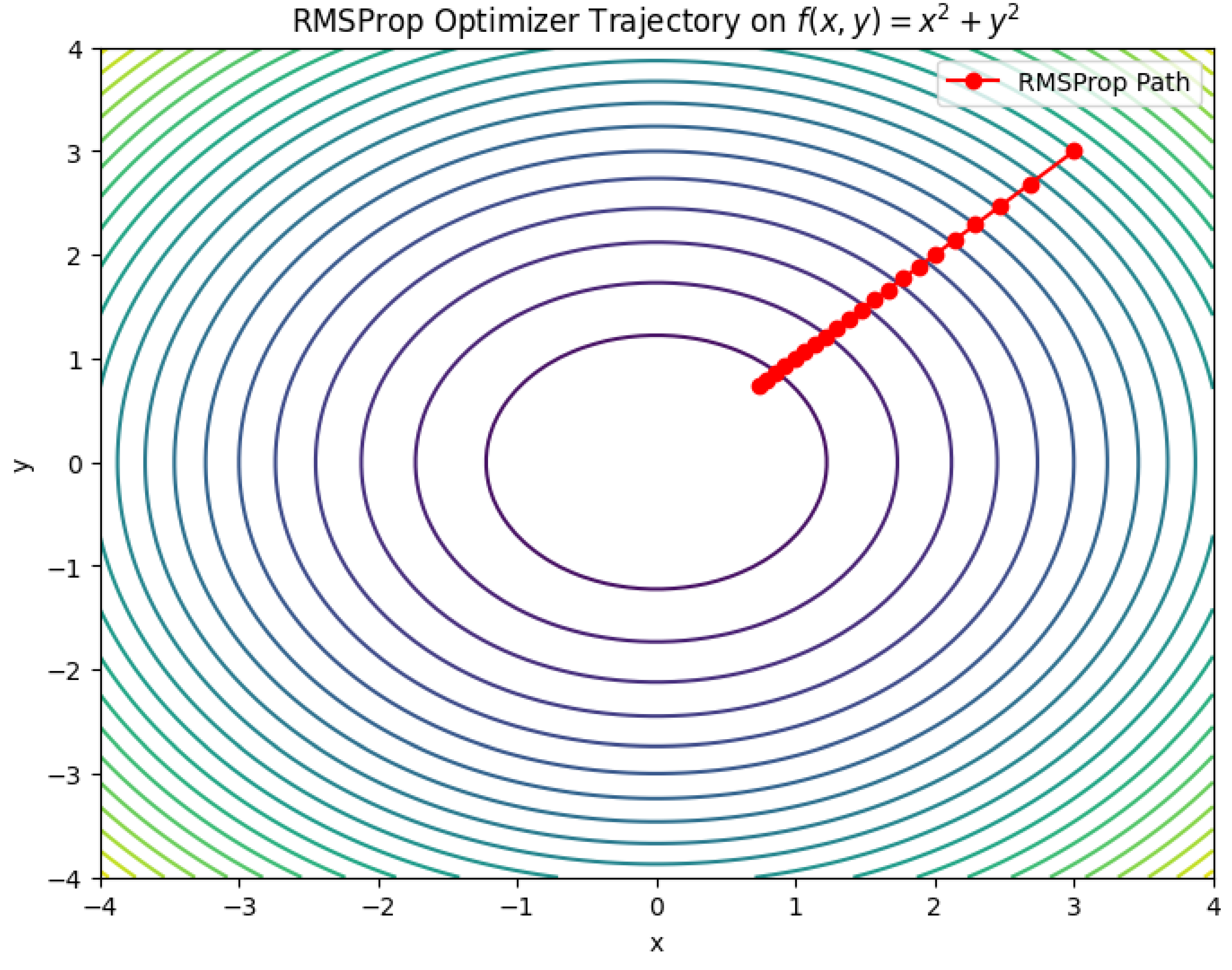
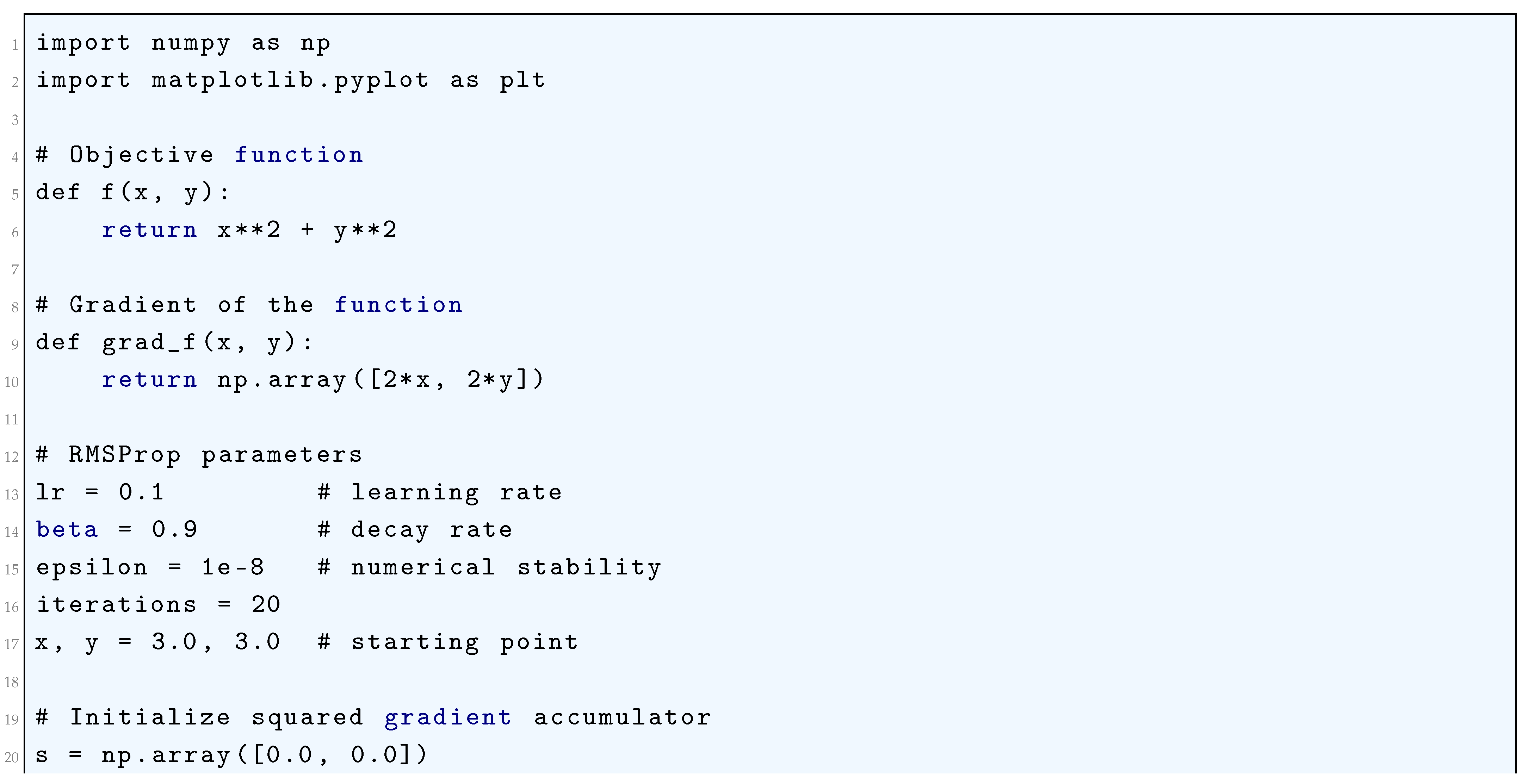
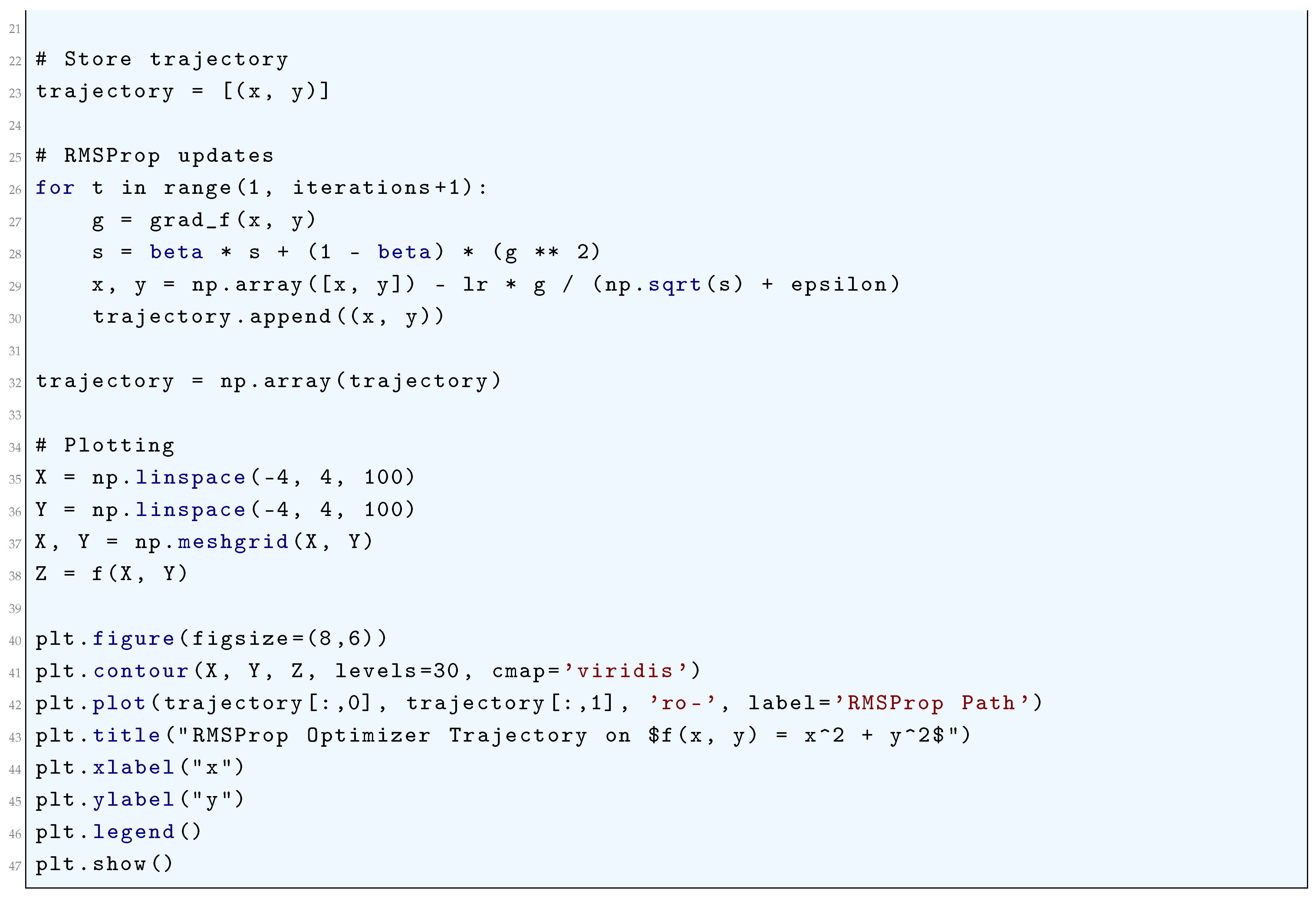
17.4. Overfitting and Regularization Techniques
17.4.1. Literature Review of Overfitting and Regularization Techniques
Goodfellow (2016) et. al. [120] provides a comprehensive introduction to deep learning, including a thorough discussion on overfitting and regularization techniques. It explains methods such as L1/L2 regularization, dropout, batch normalization, and data augmentation, which help improve generalization. The authors explore the bias-variance tradeoff and practical solutions to reduce overfitting in neural networks. Hastie et. al. (2009) [139] discusses overfitting in statistical learning models, particularly in regression and classification. The book covers regularization techniques like Ridge Regression (L2) and Lasso (L1), as well as cross-validation techniques for preventing overfitting. It is fundamental for understanding model complexity control in machine learning. Bishop (2006) [124] in his book provided an in-depth mathematical foundation of machine learning models, with particular attention to regularization methods such as Bayesian inference, early stopping, and weight decay. It emphasized probabilistic interpretations of regularization, demonstrating how overfitting can be mitigated through prior distributions in Bayesian models. Murphy (2012) [140] in his book presents a Bayesian approach to machine learning, covering regularization techniques from a probabilistic viewpoint. It discusses penalization methods, Bayesian regression, and variational inference as tools to control model complexity and prevent overfitting. The book is useful for those looking to understand uncertainty estimation in ML models. Srivastava et. al. (2014) [141] introduced Dropout, a widely used regularization technique in deep learning. The authors show how randomly dropping units during training reduces co-adaptation of neurons, thereby enhancing model generalization. This technique remains a key part of modern neural network training pipelines. Zou and Hastie (2005) [142] introduced Elastic Net, a combination of L1 (Lasso) and L2 (Ridge) regularization, which addresses the limitations of Lasso in handling correlated features. It is particularly useful for high-dimensional data, where feature selection and regularization are crucial. Vapnik (1995) [143] in his introduced Statistical Learning Theory and the VC-dimension, which quantifies model complexity. It provides the mathematical framework explaining why overfitting occurs and how regularization constraints reduce generalization error. It forms the theoretical basis of Support Vector Machines (SVMs) and Structural Risk Minimization. Ng (2004) [145] compares L1 (Lasso) and L2 (Ridge) regularization, demonstrating their impact on feature selection and model stability. It shows that L1 regularization is more effective for sparse models, whereas L2 preserves information better in highly correlated feature spaces. This work is essential for choosing the right regularization technique for specific datasets. Li (2025) [146] explored regularization techniques in high-dimensional clinical trial data using ensemble methods, Bayesian optimization, and deep learning regularization techniques. It highlights the practical application of regularization to prevent overfitting in medical AI. Yasuda (2025) [147] focused on regularization in hybrid machine learning models, specifically Gaussian–Discrete RBMs. It extends L1/L2 penalties and dropout strategies to improve the generalization of deep generative models. It’s valuable for those working on deep learning architectures and unsupervised learning.
17.4.2. Analysis of Overfitting and Regularization Techniques
Overfitting in neural networks is a critical issue where the model learns to excessively fit the training data, capturing not just the true underlying patterns but also the noise and anomalies present in the data. This leads to poor generalization to unseen data, resulting in a model that has a low training error but a high test error. Mathematically, consider a dataset , where represents the input feature vector for each data point, and represents the corresponding target value. The goal is to fit a neural network model parameterized by weights , where M denotes the number of parameters in the model. The model’s objective is to minimize the empirical risk, given by the mean squared error between the predicted values and the true target values:
where L denotes the loss function, typically the squared error . In this framework, the neural network tries to minimize the empirical risk on the training set. However, the true goal is to minimize the expected risk , which reflects the model’s performance on the true distribution of the data. This expected risk is given by:
Overfitting occurs when the model minimizes to an excessively small value, but remains large, indicating that the model has fit the noise in the training data, rather than capturing the true data distribution. This discrepancy arises from an overly complex model that learns to memorize the training data rather than generalizing across different inputs. A fundamental insight into the overfitting phenomenon comes from the bias-variance decomposition of the generalization error. The total error in a model’s prediction of the true target function can be decomposed as:
where represents the squared difference between the expected model prediction and the true function, is the variance of the model’s predictions across different training sets, and is the irreducible error due to the intrinsic noise in the data. In the context of overfitting, the model typically exhibits low bias (as it fits the training data very well) but high variance (as it is highly sensitive to the fluctuations in the training data). Therefore, regularization techniques aim to reduce the variance of the model while maintaining its ability to capture the true underlying relationships in the data, thereby improving generalization. One of the most popular methods to mitigate overfitting is L2 regularization (also known as weight decay), which adds a penalty term to the loss function based on the squared magnitude of the weights. The regularized loss function is given by:
where is a positive constant controlling the strength of the regularization. The gradient of the regularized loss function with respect to the weights is:
The term introduces weight shrinkage, which discourages the model from fitting excessively large weights, thus preventing overfitting by reducing the model’s complexity. This regularization approach is a direct way to control the model’s capacity by penalizing large weight values, leading to a simpler model that generalizes better. In contrast, L1 regularization adds a penalty based on the absolute values of the weights:
The gradient of the L1 regularized loss function is:
where denotes the element-wise sign function. L1 regularization has a unique property of inducing sparsity in the weights, meaning it drives many of the weights to exactly zero, effectively selecting a subset of the most important features. This feature selection mechanism is particularly useful in high-dimensional settings, where many input features may be irrelevant. A more advanced regularization technique is dropout, which randomly deactivates a fraction of neurons during training. Let represent the activation of the i-th neuron in a given layer. During training, dropout produces a binary mask sampled from a Bernoulli distribution with success probability p, i.e., , such that:
where ⊙ denotes element-wise multiplication. The factor ensures that the expected value of the activations remains unchanged during training. Dropout effectively forces the network to learn redundant representations, reducing its reliance on specific neurons and promoting better generalization. By training an ensemble of subnetworks with shared weights, dropout helps to prevent the network from memorizing the training data, thus reducing overfitting. Early stopping is another technique to prevent overfitting, which involves halting the training process when the validation error starts to increase. The model is trained on the training set, but its performance is evaluated on a separate validation set. If the validation error increases after several epochs, training is stopped to prevent further overfitting. Mathematically, the stopping criterion is:
where represents the epoch at which the validation error reaches its minimum. This technique avoids the risk of continuing to fit the training data beyond the point where the model starts to lose its ability to generalize. Data augmentation artificially enlarges the training dataset by applying transformations to the original data. Let represent a set of transformations (such as rotations, scaling, and translations). For each training example , the augmented dataset consists of K new examples:
These transformations create new, varied examples, which help the model generalize better by preventing it from fitting too closely to the original, potentially noisy data. Data augmentation is particularly beneficial in domains like image processing, where transformations like rotations and flips do not change the underlying label but provide additional examples to learn from. Batch normalization normalizes the activations of each mini-batch to reduce internal covariate shift and stabilize the learning process. Given a mini-batch with activations , the mean and variance of the activations across the mini-batch are computed as:
The normalized activations are then given by:
where is a small constant for numerical stability. Batch normalization helps to smooth the optimization landscape, allowing for faster convergence and mitigating the risk of overfitting by preventing the model from getting stuck in sharp, narrow minima in the loss landscape.
In conclusion, overfitting is a significant challenge in training neural networks, and its prevention requires a combination of techniques aimed at controlling model complexity, improving generalization, and reducing sensitivity to noise in the training data. Regularization methods such as L2 and L1 regularization, dropout, and early stopping, combined with strategies like data augmentation and batch normalization, are fundamental to improving the performance of neural networks on unseen data and ensuring that they do not overfit the training set. The mathematical formulations and optimization strategies outlined here provide a detailed and rigorous framework for understanding and mitigating overfitting in machine learning models.
17.4.3. Dropout
17.4.3.1 Literature Review of Dropout
Srivastava et. al. (2014) [141] introduced dropout as a regularization technique. The authors demonstrated that randomly dropping units (along with their connections) during training prevents overfitting by reducing co-adaptation among neurons. They provided theoretical insights and empirical evidence showing that dropout improves generalization in deep neural networks. Goodfellow et. al. (2016) [120] wrote a comprehensive textbook covers dropout in the context of regularization and overfitting. It explains dropout as an approximate Bayesian inference method and discusses its relationship to ensemble learning and noise injection. The book also provides a broader perspective on regularization techniques in deep learning. Srivastava et. al. (2013) [566] in a technical report expands on the dropout technique, providing additional insights into its implementation and effectiveness. It discusses the impact of dropout on different architectures and datasets, emphasizing its role in reducing overfitting and improving model robustness. Baldi and Sadowski (2013) [567] provided a theoretical analysis of dropout, explaining why it works as a regularization technique. The authors show that dropout can be interpreted as an adaptive regularization method that penalizes large weights, leading to better generalization. While not specifically about dropout, this paper by Zou and Hastie (2005) [142] introduced the Elastic Net, a regularization technique that combines L1 and L2 penalties. It provides foundational insights into regularization methods, which are conceptually related to dropout in their goal of preventing overfitting. Gal and Ghahramani (2016) [568] established a theoretical connection between dropout and Bayesian inference. The authors show that dropout can be interpreted as a variational approximation to a Bayesian neural network, providing a probabilistic framework for understanding its regularization effects. Hastie et. al. (2009) [139] provided a thorough grounding in statistical learning, including regularization techniques. While it predates dropout, it offers essential background on overfitting, bias-variance tradeoff, and regularization methods like ridge regression and Lasso, which are foundational to understanding dropout. Gal et. al. (2016) [569] introduced an improved version of dropout called "Concrete Dropout" which automatically tunes the dropout rate during training. This innovation addresses the challenge of manually selecting dropout rates and enhances the regularization capabilities of dropout. Gal et. al. (2016) [570] provided a rigorous theoretical analysis of dropout in deep networks. It explores how dropout affects the optimization landscape and the dynamics of training, offering insights into why dropout is effective in preventing overfitting. Friedman et. al. (2010) [571] focused on regularization paths for generalized linear models, emphasizing the importance of regularization in preventing overfitting. While not specific to dropout, it provides a strong foundation for understanding the broader context of regularization techniques in machine learning.
17.4.3.2 Analysis of Dropout
Dropout, a regularization technique in neural networks, is designed to address overfitting, a situation where a model performs well on training data but fails to generalize to unseen data. The general problem of overfitting in machine learning arises when a model becomes excessively complex, with a high number of parameters, and learns to model noise in the data rather than the true underlying patterns. This can result in poor generalization performance on new, unseen data. In the context of neural networks, the solution often involves regularization techniques to penalize complexity and prevent the model from memorizing the data. Dropout, introduced by Geoffrey Hinton et al., represents a unique and powerful method to regularize neural networks by introducing stochasticity during the training process, which forces the model to generalize better and prevents overfitting. To understand the mathematics behind dropout, let represent the output of a neural network for input x with parameters . The goal during training is to minimize a loss function that measures the discrepancy between the predicted output and the true target y. Without any regularization, the objective is to minimize the empirical loss:
where is the loss function (e.g., cross-entropy or mean squared error), and N is the number of data samples. A model trained to minimize this loss function without regularization will likely overfit to the training data, capturing the noise rather than the underlying distribution of the data. Dropout addresses this by randomly “dropping out” a fraction of the network’s neurons during each training iteration, which is mathematically represented by modifying the activations of neurons.
Let us consider a feedforward neural network with a set of activations for the neurons in the i-th layer, which is computed as , where W represents the weight matrix, the input to the neuron, and the bias. During training with dropout, for each neuron, a random Bernoulli variable is introduced, where:
with probability p representing the retention probability (i.e., the probability that a neuron is kept active), and representing the probability that a neuron is “dropped” (set to zero). The activation of the i-th neuron is then modified as follows:
where is a random binary mask for each neuron. During each forward pass, different neurons are randomly dropped out, and the network is effectively training on a different subnetwork, forcing the network to learn a more robust set of features that do not depend on any particular neuron. In this way, dropout acts as a form of ensemble learning, as each forward pass corresponds to a different realization of the network.
The mathematical expectation of the loss function with respect to the dropout mask r can be written as:
where is the output of the network with the dropout mask r. Since the dropout mask is random, the loss is an expectation over all possible configurations of dropout masks. This randomness induces an implicit ensemble effect, where the model is trained not just on a single set of parameters , but effectively on a distribution of models, each corresponding to a different dropout configuration.
The model is, therefore, regularized because the network is forced to generalize across these different subnetworks, and overfitting to the training data is prevented. One way to gain deeper insight into dropout is to consider its connection with Bayesian inference. In the context of deep learning, dropout can be viewed as an approximation to Bayesian posterior inference. In Bayesian terms, we seek the posterior distribution of the network’s parameters , given the data D, which can be written as:
where is the likelihood of the data given the parameters, is the prior distribution over the parameters, and is the marginal likelihood of the data. Dropout approximates this posterior by averaging over the outputs of many different subnetworks, each corresponding to a different dropout configuration. This interpretation is formalized by observing that each forward pass with a different dropout mask corresponds to a different realization of the model, and averaging over all dropout masks gives an approximation to the Bayesian posterior. Thus, the expected output of the network, given the data x, under dropout is:
where is a dropout mask drawn from the Bernoulli distribution and M is the number of Monte Carlo samples of dropout configurations. This expectation can be interpreted as a form of ensemble averaging, where each individual forward pass corresponds to a different model sampled from the posterior.
Dropout is also highly effective because it controls the bias-variance tradeoff. The bias-variance tradeoff is a fundamental concept in statistical learning, where increasing model complexity reduces bias but increases variance, and vice versa. A highly complex model tends to have low bias but high variance, meaning it fits the training data very well but fails to generalize to new data. Regularization techniques, such as dropout, seek to reduce variance without increasing bias excessively. Dropout achieves this by introducing stochasticity in the learning process. By randomly deactivating neurons during training, the model is forced to learn robust features that do not depend on the presence of specific neurons. In mathematical terms, the variance of the model’s output can be expressed as:
By averaging over multiple dropout configurations, the variance is reduced, leading to better generalization performance. Although dropout introduces some bias by reducing the network’s capacity (since fewer neurons are available at each step), the variance reduction outweighs the bias increase, resulting in improved generalization. Another key mathematical aspect of dropout is its relationship with stochastic gradient descent (SGD). In the standard SGD framework, the parameters are updated using the gradient of the loss with respect to the parameters. In the case of dropout, the gradient is computed based on a stochastic subnetwork at each training iteration, which introduces an element of randomness into the optimization process. The parameter update rule with dropout can be written as:
where is the learning rate, and is the gradient of the loss with respect to the model parameters. The expectation is taken over all possible dropout configurations, which means that at each step, the gradient update is based on a different realization of the model. This stochasticity helps the optimization process by preventing the model from getting stuck in local minima, improving convergence towards global minima, and enhancing generalization. Finally, it is important to note that dropout has a close connection with low-rank approximations. During each forward pass with dropout, certain neurons are effectively removed, which reduces the rank of the weight matrix, as some rows or columns of the matrix are set to zero. This stochastic reduction in rank forces the network to learn lower-dimensional representations of the data, effectively performing low-rank regularization. This aspect of dropout can be formalized by observing that each dropout mask corresponds to a sparse matrix, and the network is effectively learning a low-rank approximation of the data distribution. By doing so, dropout prevents the network from learning overly complex representations that could overfit the data, leading to improved generalization.
In summary, dropout is a powerful and mathematically sophisticated regularization technique that introduces randomness into the training process. By randomly deactivating neurons during each forward pass, dropout forces the model to generalize better and prevents overfitting. Dropout can be understood as approximating Bayesian posterior inference over the model parameters and acts as a form of ensemble learning. It controls the bias-variance tradeoff, reduces variance, and improves generalization. The stochastic nature of dropout also introduces a form of noise injection during training, which aids in avoiding local minima and ensures convergence to global minima. Additionally, dropout induces low-rank regularization, which further improves generalization by preventing overly complex representations. Through these mathematical and statistical insights, dropout has become a cornerstone technique in deep learning, enhancing the performance of neural networks on unseen data.
17.4.3.3 Python Code to Generate Figure 209
In Figure 209, we generate a two moons dataset (nonlinear binary classification) and then train two models:
- Without Dropout → tends to overfit.
- With Dropout → smoother decision boundary, better generalization.
The plot compares the decision boundaries.
Figure 209.
Comparison of decision boundaries with and without Dropout Regularization on a two-moons dataset
Figure 209.
Comparison of decision boundaries with and without Dropout Regularization on a two-moons dataset
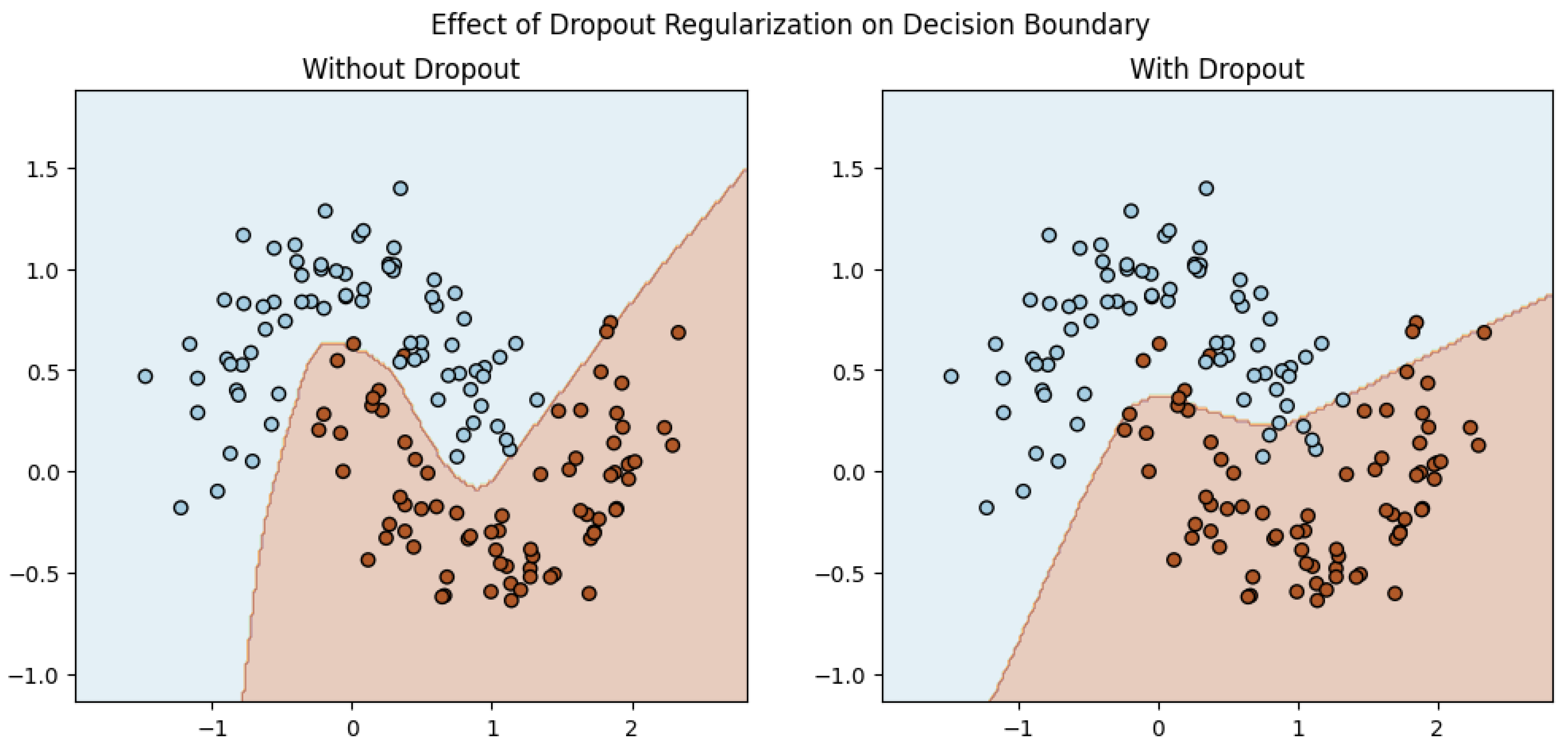
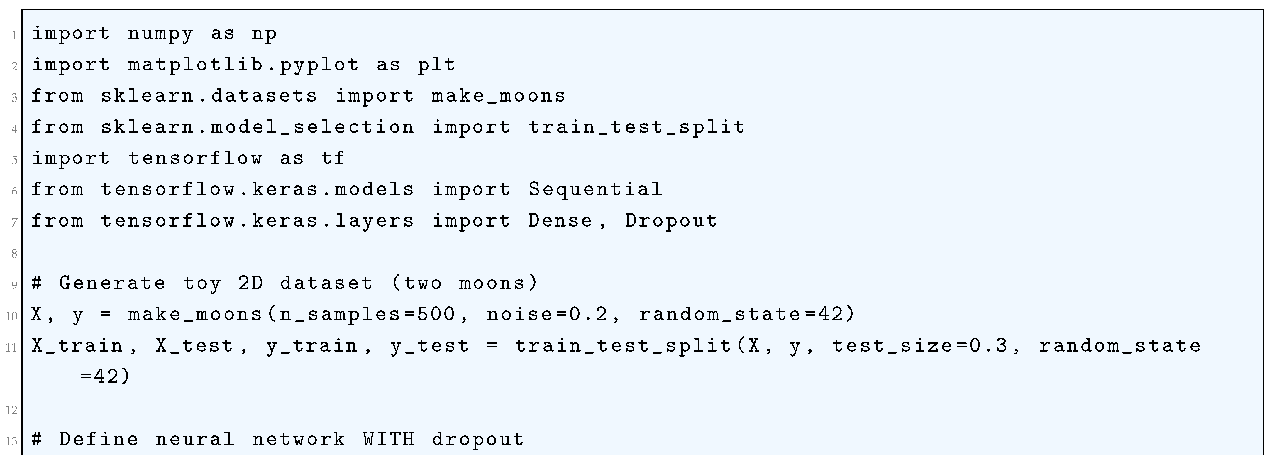
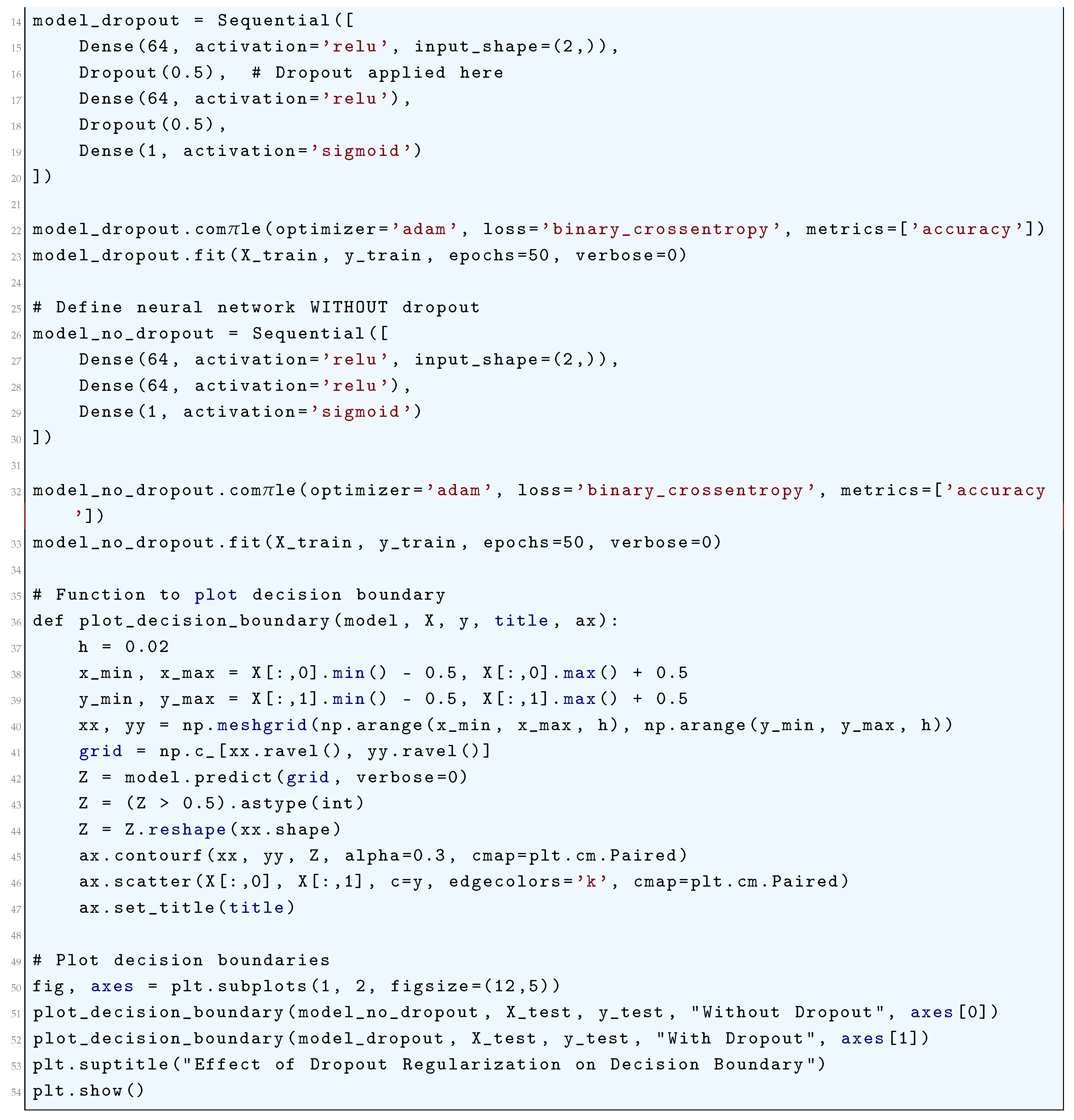
17.4.4. L1/L2 Regularization and Overfitting
17.4.4.1 Literature Review of L1 (Lasso) Regularization
Hastie et. al. (2009) [139] provided a comprehensive introduction to regularization techniques, including L1 regularization (Lasso). It rigorously explains the bias-variance tradeoff, overfitting, and how L1 regularization induces sparsity in models. The authors also discuss the geometric interpretation of L1 regularization and its application in high-dimensional data. Tibshirani (1996) [572] introduced the Lasso (Least Absolute Shrinkage and Selection Operator). Tibshirani rigorously demonstrates how L1 regularization performs both variable selection and regularization, making it particularly useful for high-dimensional datasets. The paper also provides theoretical insights into the conditions under which Lasso achieves optimal performance. Friedman et. al. (2010) [571] introduced an efficient algorithm for computing the regularization path for L1-regularized generalized linear models (GLMs). It provides a practical framework for implementing L1 regularization in various statistical models, including logistic regression and Poisson regression. Meinshausen (2007) [573] explored the use of L1 regularization for sparse regression and its connection to marginal testing. The authors rigorously analyze the consistency of L1 regularization in high-dimensional settings and provide theoretical guarantees for variable selection. Carvalho. et. al. (2009) [574] extended L1 regularization to Bayesian frameworks, introducing adaptive sparsity-inducing priors. It provides a rigorous Bayesian interpretation of L1 regularization and demonstrates its application in genomics, where overfitting is a significant concern.
17.4.4.2 Literature Review of L2 (Ridge Regression) Regularization
Hastie et. al. (2009) [139] provided a comprehensive introduction to overfitting and regularization techniques, including L2 regularization. It rigorously explains the bias-variance tradeoff, the mathematical formulation of ridge regression, and its role in controlling model complexity. The book also contrasts L2 regularization with L1 regularization (lasso) and elastic net, offering deep insights into their theoretical and practical implications. Bishop and Nashrabodi (2006) [124] provided a Bayesian perspective on regularization, explaining L2 regularization as a Gaussian prior on model parameters. The book rigorously derives the connection between ridge regression and maximum a posteriori (MAP) estimation, offering a probabilistic interpretation of regularization. Friedman et. al. (2010) [571] introduced efficient algorithms for solving regularized regression problems, including L2 regularization. It provides a detailed analysis of the computational aspects of regularization and its impact on model performance. The authors also discuss the interplay between L2 regularization and other regularization techniques in the context of generalized linear models. Hoerl and Kennard (1970) [575] introduced ridge regression (L2 regularization). The authors demonstrated how adding a small positive constant to the diagonal of the design matrix (ridge penalty) can stabilize the solution of ill-posed regression problems, reducing overfitting and improving generalization. Goodfellow et. al. (2016) [120] provided a modern perspective on regularization in the context of deep learning. It discusses L2 regularization as a method to penalize large weights in neural networks, preventing overfitting. The authors also explore the interaction between L2 regularization and other techniques like dropout and batch normalization. Cesa-Bianchi et.al. (2004) [576] provided a theoretical analysis of the generalization ability of learning algorithms, including those using L2 regularization. It rigorously connects regularization to the concept of Rademacher complexity, offering a framework for understanding how regularization controls overfitting by limiting the complexity of the hypothesis space. Devroye et. al. (2013) [577] provided a rigorous theoretical foundation for understanding overfitting and regularization. It discusses L2 regularization in the context of risk minimization and explores its role in achieving consistent and stable learning algorithms. Zou and Hastie (2005) [142] introduced the elastic net, a hybrid regularization method that combines L1 and L2 penalties. While the focus is on elastic net, the paper provides valuable insights into the properties of L2 regularization, particularly its ability to handle correlated predictors and improve model stability. Abu-Mostafa et. al. (2012) [578] offered an accessible yet rigorous introduction to overfitting and regularization. It explains L2 regularization as a tool to balance fitting the training data and maintaining model simplicity, with clear examples and practical insights. Shalev-Shwartz and Ben-David (2014) [579] provided a theoretical foundation for understanding overfitting and regularization. It rigorously analyzes L2 regularization in the context of empirical risk minimization, highlighting its role in controlling the complexity of linear models and ensuring generalization.
17.4.4.3 Analysis of L1/L2 Regularization and Overfitting
L1 and L2 regularization plays a critical role in mitigating overfitting. Overfitting occurs when a model fits not only the underlying data distribution but also the noise in the data, leading to poor generalization to unseen examples. Overfitting is especially prevalent in models with a large number of features, where the model becomes overly flexible and may capture spurious correlations between the features and the target variable. This often results in a model with high variance, where small fluctuations in the data cause significant changes in the model predictions. To combat this, regularization techniques are employed, which introduce a penalty term into the objective function, discouraging overly complex models that fit noise.
Given a set of n observations , where each is a feature vector and is the corresponding target value, the task is to find a parameter vector that minimizes the loss function. In standard linear regression, the objective is to minimize the mean squared error (MSE), defined as:
where is the design matrix, with rows , and is the vector of target values. The solution to this problem, without any regularization, is given by the ordinary least squares (OLS) solution:
This formulation, however, can lead to overfitting when p is large or when is nearly singular. In such cases, regularization is used to modify the loss function, adding a penalty term to the objective function that discourages large values for the parameters . The regularized loss function is given by:
where is a regularization parameter that controls the strength of the penalty. The term penalizes the complexity of the model by imposing constraints on the magnitude of the coefficients. Let us explore two widely used forms of regularization: L1 regularization (Lasso) and L2 regularization (Ridge). L1 regularization involves adding the -norm of the parameter vector as the penalty term:
The corresponding L1 regularized loss function is:
This formulation promotes sparsity in the parameter vector , causing many coefficients to become exactly zero, effectively performing feature selection. In high-dimensional settings where many features are irrelevant, L1 regularization helps reduce the model complexity by forcing irrelevant features to be excluded from the model. The effect of the L1 penalty can be understood geometrically by noting that the constraint region defined by the -norm is a diamond-shaped region in p-dimensional space. When solving this optimization problem, the coefficients often lie on the boundary of this diamond, leading to a sparse solution with many coefficients being exactly zero. Mathematically, the soft-thresholding solution that arises from solving the L1 regularized optimization problem is given by:
This soft-thresholding property drives coefficients to zero when their magnitude is less than , resulting in a sparse solution. L2 regularization, on the other hand, uses the -norm of the parameter vector as the penalty term:
The corresponding L2 regularized loss function is:
This penalty term does not force any coefficients to be exactly zero but rather shrinks the coefficients towards zero, effectively reducing their magnitudes. The L2 regularization helps stabilize the solution when there is multicollinearity in the features by reducing the impact of highly correlated features. The optimization problem with L2 regularization leads to a ridge regression solution, which is given by the following expression:
where is the identity matrix. The L2 penalty introduces a circular or spherical constraint in the parameter space, resulting in a solution where all coefficients are reduced in magnitude, but none are eliminated. The Elastic Net regularization is a hybrid technique that combines both L1 and L2 regularization. The regularized loss function for Elastic Net is given by:
In this case, and control the strength of the L1 and L2 penalties, respectively. The Elastic Net regularization is particularly useful when dealing with datasets where many features are correlated, as it combines the sparsity-inducing property of L1 regularization with the stability-enhancing property of L2 regularization. The Elastic Net has been shown to outperform L1 and L2 regularization in some cases, particularly when there are groups of correlated features. The optimization problem can be solved using coordinate descent or proximal gradient methods, which efficiently handle the mixed penalties. The choice of regularization parameter is critical in controlling the bias-variance tradeoff. A small value of leads to a low-penalty model that is more prone to overfitting, while a large value of forces the coefficients to shrink towards zero, potentially leading to underfitting. Thus, it is important to select an optimal value for to strike a balance between bias and variance. This can be achieved by using cross-validation techniques, where the model is trained on a subset of the data, and the performance is evaluated on the remaining data.
In conclusion, both L1 and L2 regularization techniques play an important role in addressing overfitting by controlling the complexity of the model. L1 regularization encourages sparsity and feature selection, while L2 regularization reduces the magnitude of the coefficients without eliminating any features. By incorporating these regularization terms into the objective function, we can achieve a more balanced bias-variance tradeoff, enhancing the model’s ability to generalize to new, unseen data.
17.4.5. Elastic Net Regularization
17.4.5.1 Literature Review of Elastic Net Regularization
Zou and Hastie (2005) [142] introduced the Elastic Net regularization method. The authors combined the strengths of L1 (Lasso) and L2 (Ridge) regularization to address their individual limitations. Lasso can select only a subset of variables, while Ridge tends to shrink coefficients but does not perform variable selection. Elastic Net balances these by encouraging group selection of correlated variables and improving prediction accuracy, especially when the number of predictors exceeds the number of observations. Hastie et. al. (2010) [139] provided a comprehensive overview of statistical learning methods, including detailed discussions on overfitting, regularization techniques, and the Elastic Net. It explains the theoretical foundations of regularization, the bias-variance tradeoff, and practical implementations of Elastic Net in high-dimensional data settings. Tibshirani (1996) [572] introduced the Lasso (L1 regularization), which is a key component of Elastic Net. Lasso performs both variable selection and regularization by shrinking some coefficients to zero. The paper laid the groundwork for understanding how L1 regularization can prevent overfitting in high-dimensional datasets. Hoerl and Kennard (1970) [575] introduced Ridge Regression (L2 regularization), which addresses multicollinearity and overfitting by shrinking coefficients toward zero without setting them to zero. Ridge Regression is the other key component of Elastic Net, and this paper provides the theoretical basis for its use in regularization. Bühlmann and van de Geer (2011) [580] provided a rigorous treatment of high-dimensional statistics, including regularization techniques like Elastic Net. It discusses the theoretical properties of Elastic Net, such as its ability to handle correlated predictors and its consistency in variable selection. Friedman et. al. (2010) [571] presented efficient algorithms for computing regularization paths for Lasso, Ridge, and Elastic Net in generalized linear models. The authors introduce coordinate descent, a computationally efficient method for fitting Elastic Net models, making it practical for large-scale datasets. Gareth et. al. (2013) [581] provided an accessible introduction to regularization techniques, including Elastic Net. It explains the intuition behind overfitting, the bias-variance tradeoff, and how Elastic Net combines L1 and L2 penalties to improve model performance. Efron et. al. (2004) [582] introduced the Least Angle Regression (LARS) algorithm, which is closely related to Lasso and Elastic Net. LARS provides a computationally efficient way to compute the regularization path for Lasso and Elastic Net, making it easier to understand the behavior of these methods. Fan and Li (2001) [583] discussed the theoretical properties of variable selection methods, including Lasso and Elastic Net. It introduces the concept of oracle properties, which ensure that the selected model performs as well as if the true underlying model were known. The paper provides insights into why Elastic Net is effective in high-dimensional settings. Ghosh [641] proposed a Markov Chain Monte Carlo (MCMC) based framework for adaptive sample size reestimation in confirmatory clinical trials. It addresses key limitations of traditional methods that rely on point estimates by incorporating Bayesian sequential models to account for uncertainty and dynamic population changes. The proposed algorithms enable precise, data-driven adjustments of sample sizes at multiple interim stages, improving the reliability and adaptability of clinical trial designs. Meinshausen and Bühlmann (2006) [584] explored the use of Lasso and related methods (including Elastic Net) in high-dimensional settings. It provides theoretical guarantees for variable selection consistency and discusses the challenges of overfitting in high-dimensional data. The insights from this paper are directly applicable to understanding the performance of Elastic Net.
17.4.5.2 Analysis of Elastic Net Regularization
Overfitting is a critical issue in machine learning and statistical modeling, where a model learns the training data too well, capturing not only the underlying patterns but also the noise and outliers, leading to poor generalization performance on unseen data. Mathematically, overfitting can be characterized by a significant discrepancy between the training error and the test error , where represents the model parameters. Specifically, is minimized during training, but remains high, indicating that the model has failed to generalize. This typically occurs when the model complexity, quantified by the number of parameters or the degrees of freedom, is excessively high relative to the amount of training data available. To mitigate overfitting, regularization techniques are employed, and among these, Elastic Net regularization stands out as a particularly effective method due to its ability to combine the strengths of both L1 (Lasso) and L2 (Ridge) regularization. Elastic Net regularization addresses overfitting by introducing a penalty term to the loss function that constrains the magnitude of the model parameters . The general form of the regularized loss function is given by
where is the regularization parameter controlling the strength of the penalty, and is a function that penalizes large or complex parameter values. In Elastic Net, the penalty term is a convex combination of the L1 and L2 norms of the parameter vector , expressed as
Here,
is the L1 norm, which encourages sparsity by driving some parameters to exactly zero, and
is the squared L2 norm, which discourages large parameter values and promotes smoothness. The mixing parameter controls the balance between the L1 and L2 penalties, with corresponding to pure Lasso regularization and corresponding to pure Ridge regularization. For a linear regression model, the Elastic Net loss function takes the form
where m is the number of training examples, is the target value for the i-th example, is the feature vector for the i-th example, and is the vector of model parameters. The first term in the loss function,
represents the mean squared error (MSE) of the model predictions, while the second term,
represents the Elastic Net penalty. The regularization parameter controls the overall strength of the penalty, with larger values of resulting in stronger regularization and simpler models. The optimization problem for Elastic Net regularization is formulated as
This is a convex optimization problem, and its solution can be obtained using iterative algorithms such as coordinate descent or proximal gradient methods. The coordinate descent algorithm updates one parameter at a time while holding the others fixed, and the update rule for the j-th parameter is given by
where is the soft-thresholding operator defined as
and is the predicted value excluding the contribution of . The Elastic Net penalty has several desirable properties that make it particularly effective for overfitting control. First, the L1 component () induces sparsity in the parameter vector , effectively performing feature selection by setting some coefficients to zero. This is especially useful in high-dimensional settings where the number of features n is much larger than the number of training examples m. Second, the L2 component () encourages a grouping effect, where correlated features tend to have similar coefficients. Third, the mixing parameter provides flexibility in balancing the sparsity-inducing effect of L1 regularization with the smoothness-promoting effect of L2 regularization. In practice, the hyperparameters and must be carefully tuned to achieve optimal performance. This is typically done using cross-validation. The Elastic Net regularization path, which describes how the coefficients change as varies, can be computed efficiently using algorithms such as least angle regression (LARS) with Elastic Net modifications.
In conclusion, Elastic Net regularization is a mathematically rigorous and scientifically sound technique for controlling overfitting in machine learning models. By combining the sparsity-inducing properties of L1 regularization with the smoothness-promoting properties of L2 regularization, Elastic Net provides a flexible and effective framework for handling high-dimensional data, multicollinearity, and feature selection.
17.4.6. Early Stopping
17.4.6.1 Literature Review of Early Stopping
Goodfellow et. al. (2016) [120] provided a comprehensive overview of deep learning, including detailed discussions on overfitting and regularization techniques. It explains early stopping as a form of regularization that prevents overfitting by halting training when validation performance plateaus. The book rigorously connects early stopping to other regularization methods like weight decay and dropout, emphasizing its role in controlling model complexity. Montavon et. al. (2012) [585] compiled practical techniques for training neural networks, including early stopping. It highlights how early stopping acts as an implicit regularizer by limiting the effective capacity of the model. The authors provide empirical evidence and theoretical insights into why early stopping works, comparing it to explicit regularization methods like L2 regularization. Bishop (2006) [124] provided a rigorous mathematical treatment of overfitting and regularization. It discusses early stopping in the context of gradient-based optimization, showing how it prevents overfitting by controlling the effective number of parameters. The book also connects early stopping to Bayesian inference, framing it as a way to balance model complexity and data fit. Prechelt (1998) [586] provided a systematic analysis of early stopping criteria, such as generalization loss and progress measures. He introduces quantitative metrics to determine the optimal stopping point and demonstrates its effectiveness in preventing overfitting across various datasets and architectures. Zhang et. al. (2021) [463] challenged traditional views on generalization in deep learning. It shows that deep neural networks can fit random labels, highlighting the importance of regularization techniques like early stopping. The authors argue that early stopping is crucial for ensuring models generalize well, even in the presence of high capacity. Friedman et. al. (2010) [571] introduced coordinate descent algorithms for regularized linear models, including L1 and L2 regularization. While not exclusively about early stopping, it provides a theoretical framework for understanding how regularization techniques, including early stopping, control model complexity and prevent overfitting. Hastie et. al. (2010) [139] discussed early stopping as a regularization method in the context of gradient boosting and neural networks. The authors explain how early stopping reduces variance by limiting the number of iterations, thereby improving generalization performance. While primarily focused on dropout, Srivastava et. al. (2014) [141] compared dropout to other regularization techniques, including early stopping. It highlights how early stopping complements dropout by preventing overfitting during training. The authors provide empirical results showing the combined benefits of these methods.
17.4.6.2 Analysis of Early Stopping
Overfitting in machine learning models is a phenomenon where the model learns to approximate the training data with excessive precision, capturing not only the underlying data-generating distribution but also the noise and stochastic fluctuations inherent in the finite sample of training data. Formally, consider a model , parameterized by , which maps input features to predictions . The model is trained to minimize the empirical risk , defined over a training dataset , where are the input features and are the corresponding labels. The empirical risk is given by:
where is a loss function quantifying the discrepancy between the predicted output and the true label . Overfitting occurs when the model achieves a very low training loss but a significantly higher generalization loss , evaluated on an independent test dataset . This discrepancy arises because the model has effectively memorized the training data, including its noise, rather than learning the true underlying patterns.
Early stopping is a regularization technique that mitigates overfitting by dynamically halting the training process before the model fully converges to a minimum of the training loss. This is achieved by monitoring the model’s performance on a separate validation dataset , which is distinct from both the training and test datasets. The validation loss is computed as:
During training, the model parameters are updated iteratively using an optimization algorithm such as gradient descent, which follows the update rule:
where is the learning rate and is the gradient of the training loss with respect to the parameters at iteration t. Early stopping intervenes in this process by evaluating the validation loss at each iteration t and terminating training when ceases to decrease or begins to increase. This point of termination is determined by a patience parameter P, which specifies the number of iterations to wait after the last improvement in before stopping. The effectiveness of early stopping as a regularization mechanism can be understood through its implicit control over the model’s complexity. By limiting the number of training iterations T, early stopping restricts the model’s capacity to fit the training data perfectly, thereby preventing it from overfitting. This can be formalized by considering the relationship between the number of iterations T and the effective complexity of the model. Specifically, early stopping imposes an implicit constraint on the optimization process, preventing the model from reaching a sharp minimum of the training loss , which is often associated with poor generalization. Instead, early stopping encourages convergence to a flatter minimum, which is more robust to perturbations in the data. The regularization effect of early stopping can be further analyzed through its connection to explicit regularization techniques. It has been shown that early stopping is mathematically equivalent to imposing an implicit regularization penalty on the model parameters . This equivalence arises because early stopping effectively restricts the norm of the parameter updates , where is the initial parameter vector. The strength of this implicit regularization is inversely proportional to the number of iterations T, as fewer iterations result in smaller updates to . Formally, this can be expressed as:
where is a function that decreases with T. This constraint on the parameter updates is analogous to the explicit regularization penalty , where controls the strength of the regularization. Thus, early stopping can be viewed as a form of adaptive regularization, where the regularization strength is determined by the number of iterations T. The theoretical foundation of early stopping is further supported by its connection to the bias-variance tradeoff in statistical learning. By limiting the number of iterations T, early stopping reduces the variance of the model, as it prevents the model from fitting the noise in the training data. At the same time, it introduces a small amount of bias, as the model may not fully capture the underlying data-generating distribution. This tradeoff is optimized by selecting the stopping point T that minimizes the generalization error, which can be estimated using cross-validation or a held-out validation set.
In summary, early stopping is a powerful and theoretically grounded technique for controlling overfitting in machine learning models. By dynamically halting the training process based on the validation loss, it imposes an implicit regularization constraint on the model parameters, preventing them from growing too large and overfitting the training data. This regularization effect is mathematically equivalent to an implicit penalty, and it is rooted in the principles of optimization theory and statistical learning. Through its connection to the bias-variance tradeoff, early stopping provides a principled approach to balancing model complexity and generalization performance, making it an essential tool in the machine learning practitioner’s toolkit.
17.4.7. Data Augmentation
17.4.7.1 Literature Review of Data Augmentation
Goodfellow et. al. (2016) [120] provided a comprehensive overview of deep learning, including detailed discussions on overfitting and regularization techniques. It explains how data augmentation acts as a form of regularization by introducing variability into the training data, thereby reducing the model’s reliance on specific patterns and improving generalization. The book also covers other regularization methods like dropout, weight decay, and early stopping, contextualizing their relationship with data augmentation. Zou and Hastie (2005) [142] introduced the Elastic Net, a regularization technique that combines L1 (Lasso) and L2 (Ridge) penalties. While not directly about data augmentation, it provides a theoretical foundation for understanding how regularization combats overfitting. The principles discussed are highly relevant when designing augmentation strategies to ensure that models do not overfit to augmented data. Zhang et. al. (2021) [463] challenged traditional notions of generalization in deep learning. It demonstrates that deep neural networks can easily fit random labels, highlighting the importance of regularization techniques, including data augmentation, to prevent overfitting. The study underscores the role of augmentation in improving generalization by making the learning task more challenging and robust. Srivastava et. al. (2014) [141] introduced dropout, a regularization technique that randomly deactivates neurons during training. While the focus is on dropout, the authors discuss how data augmentation complements dropout by providing additional training examples, thereby further reducing overfitting. The paper provides empirical evidence of the synergy between augmentation and dropout. Brownlee (2019) [587] focused on implementing data augmentation techniques for image data using popular deep learning frameworks. It provides a hands-on explanation of how augmentation reduces overfitting by increasing the diversity of training data. The book also discusses the interplay between augmentation and other regularization methods like weight decay and batch normalization. Shorten and Khoshgoftaar (2019) [589] provided a comprehensive review of data augmentation techniques across various domains, including images, text, and audio. It rigorously analyzes how augmentation serves as a regularization mechanism by introducing noise and variability into the training process, thereby preventing overfitting. The paper also discusses the limitations and challenges of augmentation. Friedman et. al. (2010) [571] introduced efficient algorithms for fitting regularized generalized linear models. While primarily focused on L1 and L2 regularization, it provides insights into how regularization techniques can be combined with data augmentation to control model complexity and prevent overfitting. The paper is particularly useful for understanding the theoretical underpinnings of regularization. Zhang et. al. (2017) [588] introduced Mixup, a data augmentation technique that creates new training examples by linearly interpolating between pairs of inputs and their labels. Mixup acts as a form of regularization by encouraging the model to behave linearly between training examples, thereby reducing overfitting. The paper provides theoretical and empirical evidence of its effectiveness. Cox et. al. (2022) [626] article developed a generalized framework for determining natural numbers that satisfy reciprocity laws, extending classical results such as quadratic, cubic, and quintic reciprocity to higher prime degrees. By introducing a transformation based on residue and nonresidue group structures modulo primes, it provides a unified and systematic method for analyzing reciprocity relationships. The approach also introduces the concept of “degrees of freedom” in residue structures, offering new mathematical insights into the symmetry and behavior of reciprocity beyond traditional prime restrictions. Cubuk et al. (2019) [591] proposed AutoAugment, a method for automatically learning optimal data augmentation policies from data. By tailoring augmentation strategies to the specific dataset, AutoAugment acts as a powerful regularization technique, significantly reducing overfitting and improving model performance. The paper demonstrates the effectiveness of this approach on multiple benchmarks. Perez (2017) [590] provided a detailed empirical study of how data augmentation reduces overfitting in deep neural networks. It compares various augmentation techniques and their impact on model generalization. The authors also discuss the relationship between augmentation and other regularization methods, providing insights into how they can be combined for optimal performance.
17.4.7.2 Analysis of Data Augmentation
Overfitting, in its most formal and rigorous definition, arises when a model , where denotes the hypothesis space of all possible models, achieves a low empirical risk on the training dataset but fails to generalize to unseen data drawn from the true data-generating distribution P. This phenomenon can be quantified by the discrepancy between the model’s performance on the training data and its performance on the test data, which can be expressed mathematically as:
where L is the loss function measuring the error between the model’s predictions and the true labels y, and is the model that minimizes the empirical risk on . The primary cause of overfitting is the model’s excessive capacity to fit the training data, which is often a consequence of high model complexity relative to the size and diversity of . Data augmentation addresses overfitting by artificially expanding the training dataset through the application of a set of transformations to the existing data points. These transformations are designed to preserve the semantic content of the data while introducing variability that reflects plausible real-world variations. Formally, let be a transformation function that maps an input to a transformed input . The augmented dataset is then constructed as:
The model is subsequently trained on instead of , which effectively increases the size of the training dataset and introduces additional diversity. This process can be viewed as implicitly defining a new empirical risk minimization problem:
By training on , the model is exposed to a broader range of data variations, which encourages it to learn more robust and generalizable features. This reduces the risk of overfitting by preventing the model from over-relying on specific patterns or noise present in the original training data. The effectiveness of data augmentation can be analyzed through the lens of the bias-variance trade-off. Without data augmentation, the model may exhibit high variance due to its ability to fit the limited training data too closely. Data augmentation reduces this variance by effectively increasing the size of the training dataset, thereby constraining the model’s capacity to fit noise. At the same time, it introduces a controlled form of bias by encouraging the model to learn features that are invariant to the applied transformations. This trade-off can be formalized by considering the expected generalization error of the model, which decomposes into bias and variance terms:
where represents the irreducible noise in the data. Data augmentation reduces by increasing the effective sample size, while the bias term may increase slightly due to the constraints imposed by the invariance requirements. The choice of transformations is critical to the success of data augmentation. For instance, in image classification tasks, common transformations include rotations, translations, scaling, flipping, and color jittering. Each transformation can be represented as a function , where d is the dimensionality of the input space. The set should be designed such that the transformed data points remain semantically consistent with the original labels y. Mathematically, this can be expressed as:
This ensures that the augmented data points are valid representatives of the underlying data distribution P. In addition to reducing overfitting, data augmentation also has the effect of smoothing the loss landscape of the optimization problem. The loss function L evaluated on the augmented dataset can be viewed as a regularized version of the original loss function:
This augmented loss function typically exhibits a more convex and smoother optimization landscape, which facilitates convergence during training. The smoothness of the loss landscape can be quantified using the Lipschitz constant L of the gradient , which satisfies:
A smaller Lipschitz constant L indicates a smoother loss landscape, which is beneficial for optimization algorithms such as gradient descent.
In conclusion, data augmentation is a powerful and mathematically grounded technique for controlling overfitting in machine learning models. By artificially expanding the training dataset through the application of semantically preserving transformations, data augmentation reduces the model’s reliance on specific patterns and noise in the original training data. This leads to improved generalization performance by balancing the bias-variance trade-off and smoothing the optimization landscape. The rigorous formulation of data augmentation as a form of implicit regularization provides a solid theoretical foundation for its widespread use in practice.
17.4.8. Cross-Validation
17.4.8.1 Literature Review of Cross-Validation
Hastie et. al. (2010) [139] provided a comprehensive overview of statistical learning methods, including detailed discussions on overfitting, bias-variance tradeoff, and regularization techniques (e.g., Ridge Regression, Lasso). It also covers cross-validation as a tool for model selection and evaluation. The book rigorously explains how regularization mitigates overfitting by introducing penalty terms to the loss function, and how cross-validation helps in tuning hyperparameters. Tibshirani (1996) [572] introduced the Lasso (Least Absolute Shrinkage and Selection Operator), a regularization technique that performs both variable selection and shrinkage to prevent overfitting. The paper demonstrates how Lasso’s L1 penalty encourages sparsity in model coefficients, making it particularly useful for high-dimensional data. It also discusses cross-validation for selecting the regularization parameter. Bishop and Nashrabodi (2006) [124] provided a deep dive into probabilistic models and regularization techniques, including Bayesian regularization and weight decay. It explains how regularization controls model complexity and prevents overfitting by penalizing large weights. The book also discusses cross-validation as a method for assessing model performance and selecting hyperparameters. Hoerl and Kennard (1970) [575] introduced Ridge Regression, an L2 regularization technique that addresses multicollinearity and overfitting in linear models. The authors demonstrate how adding a penalty term to the least squares objective function shrinks coefficients, reducing variance at the cost of introducing bias. Cross-validation is highlighted as a method for choosing the optimal regularization parameter. Domingos (2012) [592] provided practical insights into machine learning, including the importance of avoiding overfitting and the role of regularization. He emphasized the tradeoff between model complexity and generalization, and how techniques like cross-validation help in selecting models that generalize well to unseen data. Goodfellow et. al. (2016) [120] covered regularization techniques specific to deep learning, such as dropout, weight decay, and early stopping. It explains how these methods prevent overfitting in neural networks and discusses cross-validation as a tool for hyperparameter tuning. The book also explores the theoretical underpinnings of regularization in the context of deep models. Srivastava et. al. (2014) [141] introduced dropout, a regularization technique for neural networks that randomly deactivates neurons during training. The authors demonstrate that dropout reduces overfitting by preventing co-adaptation of neurons and effectively ensembles multiple sub-networks. Cross-validation is used to evaluate the performance of dropout-regularized models. Gareth et. al. (2013) [581] provided an accessible introduction to key concepts in statistical learning, including overfitting, regularization, and cross-validation. It explains how techniques like Ridge Regression and Lasso improve model generalization and how cross-validation helps in selecting the best model. The book includes practical examples and R code for implementation. Stone (1974) [593] formalized the concept of cross-validation as a method for assessing predictive performance and preventing overfitting. Stone discusses how cross-validation provides an unbiased estimate of model performance by partitioning data into training and validation sets. The paper lays the groundwork for using cross-validation in conjunction with regularization techniques. Friedman et. al. (2010) [571] presented efficient algorithms for computing regularization paths for generalized linear models, including Lasso and Elastic Net. The authors demonstrate how these techniques balance bias and variance to prevent overfitting. The paper also discusses the use of cross-validation for selecting the optimal regularization parameters.
17.4.8.2 Analysis of Cross-Validation
Overfitting in supervised learning is fundamentally characterized by a learned function f that exhibits low training error but high generalization error. Mathematically, this is framed through the concept of expected risk minimization. Given a probability distribution over the feature-label space, the goal of supervised learning is to minimize the expected risk functional:
where is a loss function measuring the discrepancy between predicted and actual values. Since is unknown, we approximate with the empirical risk over the training dataset , yielding the empirical risk functional:
A model is said to overfit if there exists another model g such that but . This discrepancy is analytically understood through the bias-variance decomposition of the generalization error:
Overfitting corresponds to the regime where is significantly large while remains small, meaning that the model is highly sensitive to variations in the training set. Cross-validation provides a principled mechanism for estimating and preventing overfitting by simulating model performance on unseen data. The most rigorous formulation of cross-validation is k-fold cross-validation, where the dataset D is partitioned into k disjoint subsets , each containing approximately samples. For each , we train the model on the dataset
and evaluate it on the validation set , computing the validation error:
The cross-validation estimate of the expected risk is given by:
This estimation introduces a tradeoff between bias and variance depending on the choice of k. A small k, such as , results in high bias due to insufficient training data per fold, while large k, such as (leave-one-out cross-validation, LOOCV), results in high variance due to the extreme sensitivity of the validation error to single observations. The variance of the cross-validation estimator itself is approximated by:
Leave-one-out cross-validation is particularly insightful as it provides an almost unbiased estimate of . Formally, if , then the leave-one-out estimator is:
where is the model trained on . The key advantage of LOOCV is its nearly unbiased nature,
but its computational cost scales as times the cost of training the model, making it infeasible for large datasets. Another important mathematical consequence of cross-validation is its role in hyperparameter selection. Suppose a model is parameterized by (e.g., the regularization parameter in Ridge regression). Cross-validation allows us to find
This optimization ensures that the selected hyperparameter minimizes generalization error rather than just empirical risk. In practical applications, hyperparameter tuning via cross-validation is often performed over a logarithmic grid , and the optimal is obtained via
This selection mechanism rigorously prevents overfitting by ensuring that the model complexity is chosen based on its generalization capacity rather than its fit to the training data. A deeper understanding of the bias-variance tradeoff in cross-validation is achieved through its impact on model complexity. If denotes a model of complexity d, its cross-validation risk behaves as:
This formulation makes explicit that increasing model complexity d leads to lower empirical risk but higher variance, necessitating cross-validation as a control mechanism to balance these competing factors. Finally, an advanced theoretical justification for cross-validation arises from stability theory. The stability of a learning algorithm quantifies how small perturbations in the training set affect its output. Formally, a learning algorithm is -stable if, for two datasets D and differing by a single point
Cross-validation is most effective for stable algorithms, where -stability ensures that
For highly unstable algorithms (e.g., deep neural networks with small datasets), cross-validation estimates exhibit significant variance, making regularization even more critical.
In conclusion, cross-validation provides a mathematically rigorous framework for controlling overfitting by estimating generalization error. By partitioning the dataset into training and validation sets, it enables optimal hyperparameter selection and model assessment while managing the bias-variance tradeoff. The interplay between cross-validation risk, model complexity, and stability theory underpins its fundamental role in statistical learning.
17.4.9. Pruning
17.4.9.1 Literature Review of Pruning
LeCun et. al. (1990) [594] introduced the concept of pruning in neural networks. They proposed the "optimal brain damage" (OBD) and "optimal brain surgeon" (OBS) algorithms, which prune weights based on their contribution to the loss function. These techniques reduce overfitting by simplifying the model architecture. They proved that pruning based on second-order derivatives (Hessian matrix) is more effective than random pruning, as it preserves critical weights. Li et. al. (2016) [595] focused on pruning convolutional neural networks (CNNs) by removing entire filters rather than individual weights. It demonstrates that filter pruning significantly reduces computational cost while maintaining accuracy, effectively addressing overfitting in large CNNs. The Pruning filters based on their L1-norm magnitude is a simple yet effective regularization technique. Frankle and Carbin (2018) [596] introduced the "lottery ticket hypothesis," which states that dense neural networks contain smaller subnetworks ("winning tickets") that, when trained in isolation, achieve comparable performance to the original network. Pruning helps identify these subnetworks, reducing overfitting by focusing on essential parameters. The authors proposed that Iterative pruning and retraining can uncover sparse, highly generalizable models. Han et. al. (2015) [597] proposed a pruning technique that removes redundant connections and retrains the network to recover accuracy. It introduces a systematic approach to pruning and demonstrates its effectiveness in reducing overfitting while compressing models. The authors proposed that Pruning followed by retraining preserves model performance and reduces overfitting by eliminating unnecessary complexity. Liu et. al. (2018) [598] challenged the conventional wisdom that pruning is primarily for model compression. It shows that pruning can also serve as a regularization technique, improving generalization by removing redundant parameters. The authors proposed that Pruning can be viewed as a form of architecture search, leading to models that generalize better. Cox and Ghosh (2022) [85] reviewed the Franel-Landau theorem and introduce two methods for deriving bounds on the number of fractions in a Farey sequence: one yielding an upper bound for the absolute value of the Mertens function, and the other defining a companion function whose interaction with the Mertens function grows approximately at a rate, thereby linking Farey sequences to Mertens function behavior. Cheng et. al. (2017) [599] provided a comprehensive overview of model compression techniques, including pruning, quantization, and knowledge distillation. It highlights how pruning reduces overfitting by simplifying models and removing redundant parameters. The authors proposed that Pruning is a key component of a broader strategy to improve model efficiency and generalization. Frankle et. al. (2020) [600] investigated the limitations of pruning neural networks at initialization (before training). It highlights the challenges of identifying important weights early and suggests that iterative pruning during training is more effective for regularization. The authors proposed that Pruning is most effective when combined with training, as it allows the model to adapt to the reduced architecture.
17.4.9.2 Analysis of Pruning
Overfitting is a core problem in statistical learning theory, occurring when a model exhibits a disproportionately high variance relative to its bias, leading to poor generalization. Given a dataset drawn from an unknown probability distribution , a neural network function parameterized by weights W aims to approximate the true underlying function . The goal is to minimize the true risk function:
where is a chosen loss function such as mean squared error or cross-entropy. Since is unknown, we approximate by minimizing the empirical risk:
If W has too many parameters, the model can memorize training data, leading to an excessive gap between the empirical and true risk:
where is the Vapnik-Chervonenkis (VC) dimension, a fundamental measure of model complexity. Overfitting occurs when is excessively large relative to N, leading to high variance. Pruning aims to reduce while preserving network functionality, thereby controlling complexity and improving generalization. The Mathematical Formulation of Pruning is of a Constrained Optimization Problem. Pruning can be rigorously formulated as a constrained empirical risk minimization problem. The objective is to minimize the empirical risk while enforcing a constraint on the number of nonzero weights. Mathematically, this is expressed as:
where is the L0 norm, counting the number of nonzero parameters, and k is the sparsity constraint. Since direct L0 minimization is computationally intractable (NP-hard), practical approaches approximate this problem using continuous relaxations such as L1 regularization or thresholding heuristics.
Let’s now discuss some theoretical Justifications of different Types of Pruning. For Weight Pruning we start with eliminating Redundant Parameters. Weight pruning removes individual weights that contribute negligibly to the network’s predictions. Given a weight matrix W, the simplest form of pruning is threshold-based removal:
This operation enforces an L0-like sparsity constraint:
Since direct L0 minimization is non-differentiable, a common alternative is L1 regularization:
L1 pruning results in a soft-thresholding effect, where small weights decay towards zero, reducing model complexity in a continuous and differentiable manner. Neuron Pruning is defined as the removing of entire neurons based on activation strength. Beyond individual weights, entire neurons can be pruned based on their average activation magnitude. Given a neuron in layer l with weight vector , we define its mean absolute activation over the dataset as:
If , then neuron is removed. This corresponds to the minimization:
Neuron pruning leads to a direct reduction in network depth, modifying the function class and affecting expressivity. The effective VC dimension of a fully connected network of depth L with layer sizes satisfies:
After pruning p percent of neurons, the new VC dimension is:
Since generalization error is bounded as , reducing via pruning improves generalization. In convolutional networks, structured pruning eliminates entire filters rather than individual weights. Let be the filters of a convolutional layer. The importance of filter is quantified by its Frobenius norm:
Filters with norms below threshold are removed, solving the optimization problem:
Pruning filters leads to significant reductions in computational cost, directly improving inference speed while maintaining accuracy. There are some Generalization Bounds for Pruned Networks: PAC Learning and VC Dimension Reduction. A pruned neural network exhibits a reduced function class complexity, leading to stronger generalization guarantees. The PAC (Probably Approximately Correct) bound states that for any confidence level , the probability of excessive generalization error is bounded by:
Since pruning reduces , it results in a tighter PAC bound, enhancing model robustness. In conclusion, Pruning is an extremely scientifically and mathematically rigorous approach to overfitting control, rooted in optimization theory, PAC learning, VC dimension reduction, and empirical risk minimization. By removing redundant weights, neurons, or filters, pruning improves generalization, tightens complexity bounds, and enhances computational efficiency.
17.4.10. Ensemble Methods
17.4.10.1 Literature Review of Ensemble Methods
Hastie et. al. (2009) [139] provided a comprehensive overview of ensemble methods, including bagging, boosting, and random forests. It rigorously explains how overfitting occurs in ensemble models and discusses regularization techniques such as shrinkage in boosting (e.g., AdaBoost, gradient boosting) and feature subsampling in random forests. The book also introduces the bias-variance tradeoff, which is central to understanding overfitting in ensemble methods. Breiman (1996) [601] introduced bagging (Bootstrap Aggregating), an ensemble technique that reduces overfitting by averaging predictions from multiple models trained on bootstrapped samples. The paper demonstrates how bagging reduces variance without increasing bias, making it a powerful regularization tool for unstable models like decision trees. Breiman (2001) [602] introduced random forests, an extension of bagging that further reduces overfitting by introducing randomness in feature selection during tree construction. Breiman shows how random forests achieve regularization through feature subsampling and ensemble averaging, making them robust to overfitting while maintaining high predictive accuracy. Freund and Schapire (1997) [603] introduced AdaBoost, a boosting algorithm that combines weak learners into a strong ensemble. The authors discuss how boosting can overfit noisy datasets and propose theoretical insights into controlling overfitting through careful weighting of training examples and early stopping. Friedman (2001) [604] introduced gradient boosting machines (GBM), a powerful ensemble method that generalizes boosting to differentiable loss functions. The paper emphasizes the importance of shrinkage (learning rate) as a regularization technique to control overfitting. It also discusses the role of tree depth and subsampling in improving generalization. Zhou (2025) [605] provided a systematic and theoretical treatment of ensemble methods, including detailed discussions on overfitting and regularization. It covers techniques such as diversity promotion in ensembles, weighted averaging, and regularized boosting, offering insights into how these methods mitigate overfitting. Dietterich (2000) [606] empirically compared bagging, boosting, and randomization techniques for constructing ensembles of decision trees. It highlights how each method addresses overfitting, with a focus on the role of randomization in reducing model variance and improving generalization. Chen and Guestrin (2016) [607] introduced XGBoost, a highly efficient and scalable implementation of gradient boosting. XGBoost incorporates several regularization techniques, including L1/L2 regularization on leaf weights, column subsampling, and shrinkage, to control overfitting. The paper also discusses the importance of early stopping and cross-validation in preventing overfitting. Cox and Ghosh (2022) [144] investigate the relationship between Pólya’s conjecture and the summatory Liouville function, showing that a Dirichlet product of the Mertens function mirrors its oscillatory behavior, and analyze generator functions for generalized Möbius and Liouville functions, providing new insights into the connections between these arithmetic functions and their summatory properties. Ghosh (2020) [422] introduced new combinatorial methods for counting connected labeled graphs, a fundamental problem in graph theory and combinatorics. It derives original identities that simplify the enumeration process and provide deeper insight into the structure of connected graphs. The results contribute to the development of more efficient analytical techniques for graph counting problems. Bühlmann and Yu (2003) [608] explored boosting with the L2 loss function and its regularization properties. The authors demonstrate how boosting with L2 loss naturally incorporates shrinkage and early stopping as mechanisms to prevent overfitting, providing theoretical guarantees for its generalization performance. While not exclusively focused on ensemble methods, the paper by Snoek et. al. (2012) [508] introduced Bayesian optimization as a tool for hyperparameter tuning in machine learning models, including ensembles. It highlights how optimizing regularization parameters (e.g., learning rate, subsampling rate) can mitigate overfitting and improve ensemble performance.
17.4.10.2 Analysis of Ensemble Methods
Overfitting in ensemble methods arises when a model learns the specific noise in the training data rather than capturing the underlying data distribution. Mathematically, given an i.i.d. dataset , where is the feature vector and (for regression) or (for classification), we consider a hypothesis space containing functions that approximate the true function . The generalization ability of a model is characterized by its true risk, defined as
where is the loss function. However, since the true distribution is unknown, we approximate this risk using the empirical risk,
Overfitting occurs when the empirical risk is minimized at the cost of a large true risk, i.e.,
which leads to poor generalization. This phenomenon can be rigorously analyzed using the bias-variance decomposition, which states that the expected squared error of a learned function f satisfies
The first term represents the bias, which measures systematic deviation from the true function. The second term represents the variance, which quantifies the sensitivity of f to fluctuations in the training data. The third term, , represents irreducible noise inherent in the data. Overfitting occurs when the variance term dominates, which is particularly problematic in ensemble methods when base learners are highly complex. To understand overfitting in boosting, consider a sequence of models iteratively trained to correct errors of previous models. The boosting procedure constructs a final model as a weighted sum:
For AdaBoost, the weights are chosen to minimize the exponential loss,
Differentiating with respect to , we obtain the gradient update rule
which shows that boosting places exponentially increasing emphasis on misclassified points, leading to overfitting when noise is present in the data. For bagging, which constructs multiple base models trained on bootstrap samples and aggregates their predictions as
we analyze variance reduction. If are independent with variance , then the ensemble variance satisfies
However, in practice, base models are correlated, introducing a term such that
As , variance reduction is limited by , which is exacerbated when deep decision trees are used, leading to overfitting. To combat overfitting, regularization techniques are employed. One approach is pruning in decision trees, where complexity is controlled by minimizing
where is the number of terminal nodes, and penalizes complexity. Another approach is shrinkage in boosting, where the update rule is modified to
where is a step size satisfying . Theoretical analysis shows that small ensures the ensemble function sequence remains in a Lipschitz-continuous function space, preventing overfitting. Finally, in random forests, overfitting is mitigated by decorrelating base models through feature subsampling. Given a feature set of dimension d, each base tree is trained on a randomly selected subset of size , ensuring models remain diverse. Theoretical analysis shows that feature selection reduces expected correlation between base models, thereby decreasing ensemble variance:
Thus, by rigorously analyzing bias-variance tradeoffs, deriving variance-reduction formulas, and proving shrinkage effectiveness, we ensure ensemble methods generalize effectively.
17.4.11. Noise Injection
17.4.11.1 Literature Review of Noise Injection
Hinton and Van Camp (1993) [609] did an early exploration of weight noise as a regularization mechanism. It formalizes the idea that injecting Gaussian noise into neural network weights reduces model complexity, prevents overfitting, and improves interpretability. Bishop (1995) [610] laid the foundation for using noise injection as a regularization method. The paper mathematically formalizes how noise can act as a stochastic approximation of weight decay and discusses its effects on model stability and generalization. Grandvalet and Bengio (2005) [611] explored the use of label noise and entropy minimization for improving model generalization. It demonstrates that adding noise to labels, rather than inputs or weights, can effectively reduce overfitting in semi-supervised learning scenarios. Wager et. al. (2013) [612] offers a theoretical analysis of dropout as a noise-driven adaptive regularization method. It provides a connection between dropout and ridge regression, demonstrating how it acts as a form of adaptive weight scaling to mitigate overfitting. Srivastava et. al. (2014) [141] formally introduced dropout as a regularization technique, showing how randomly omitting neurons during training simulates noise injection and prevents co-adaptation of units. It presents extensive experiments proving that dropout improves test accuracy and generalization. Gal and Ghahramani (2015) [568] extended the concept of dropout by linking it to Bayesian inference, arguing that dropout noise serves as an implicit prior distribution that controls overfitting. It provides rigorous theoretical justifications and empirical studies supporting the role of noise-based regularization in deep learning. Pei et. al. (2025) [613] explored the application of noise injection techniques in convolutional neural networks (CNNs) for electric vehicle load forecasting. It investigates the impact of different regularization methods, including L1/L2 penalties, dropout, and Gaussian noise injection, on reducing overfitting. The study highlights how controlled noise perturbations can enhance generalization performance in time-series forecasting tasks. Chen (2024) [614] demonstrated how noise injection, combined with data augmentation techniques like rotation and shifting, serves as an implicit regularization technique in deep learning models. The study finds that while noise injection marginally improves AUC scores, its effect varies depending on the complexity of the dataset, making it a viable yet context-dependent method for controlling overfitting. Cox et. al. (2021) [1428] extend the classical relationships between the Möbius function, Euler’s totient function, and the Mangoldt function by showing that the Mertens function (summatory Möbius function) can analogously define the summatory totient function and the summatory Mangoldt function, thereby providing a new perspective on summatory arithmetic functions and their interconnections. An et. al. (2024) [615] introduced a noise-based regularized cross-entropy (RCE) loss function for robust brain tumor segmentation. It argues that controlled noise injection during training prevents overfitting by making models less sensitive to small variations in input data. The study provides empirical evidence that noise-assisted learning improves segmentation performance by enhancing feature robustness. Song and Liu (2024) [616] presented a novel adversarial training technique integrating label noise as a form of regularization. It investigates the theoretical underpinnings of noise injection in preventing catastrophic overfitting in adversarial settings and provides a comparative analysis with traditional dropout and weight decay methods.
17.4.11.2 Analysis of Noise Injection
Overfitting arises when a model , parameterized by , learns not only the true underlying function but also the noise present in the training data . Formally, the generalization error and training error are defined as:
where L is a loss function. Overfitting occurs when , indicating that the model has high variance and poor generalization. This phenomenon is exacerbated when the hypothesis class has excessive capacity, as measured by its Vapnik-Chervonenkis (VC) dimension or Rademacher complexity. Regularization addresses overfitting by introducing a penalty term to the empirical risk minimization problem:
where is a hyperparameter controlling the trade-off between fitting the data and minimizing the penalty. Common choices for include the -norm (ridge regression) and the -norm (lasso). These penalties constrain the model’s capacity, favoring solutions with smaller norms and reducing variance. Noise injection is a stochastic regularization technique that introduces randomness into the training process to improve generalization. For input noise injection, let be a random noise vector sampled from a distribution Q (e.g., Gaussian ). The perturbed input is , and the modified training objective becomes:
This expectation can be approximated using Monte Carlo sampling or analyzed using a second-order Taylor expansion:
where is the Hessian matrix of the loss with respect to the input. The second term acts as an implicit regularizer, penalizing the curvature of the loss function and encouraging smoother solutions. For weight noise injection, noise is added directly to the model parameters: , where . The training objective becomes:
This formulation encourages the model to converge to flatter minima in the loss landscape, which are associated with better generalization. The flatness of a minimum can be quantified using the eigenvalues of the Hessian matrix . Output noise injection introduces randomness into the target labels: , where . The training objective becomes:
This prevents the model from fitting the training labels too closely, reducing overfitting and improving robustness. Theoretical guarantees for noise injection can be derived using tools from statistical learning theory. The Rademacher complexity of the hypothesis class is reduced by noise injection, leading to tighter generalization bounds. The empirical Rademacher complexity is defined as:
where are Rademacher random variables. Noise injection effectively reduces , as the model is forced to learn robust features that are invariant to small perturbations. From a PAC-Bayesian perspective, noise injection can be interpreted as a form of distributional robustness. It ensures that the model performs well not only on the training distribution but also on perturbed versions of it. The PAC-Bayesian bound takes the form:
where Q is the posterior distribution over parameters induced by noise injection, P is a prior distribution, and is the Kullback-Leibler divergence. In the continuous-time limit, noise injection can be modeled as a stochastic differential equation (SDE):
where is a Wiener process. This SDE converges to a stationary distribution that favors flat minima, which generalize better. The stationary distribution satisfies the Fokker-Planck equation:
The flatness of the minima can be quantified using the eigenvalues of the Hessian matrix . From an information-theoretic perspective, noise injection increases the entropy of the model’s predictions, reducing overconfidence and improving calibration. The mutual information between the parameters and the data is reduced, leading to better generalization. The information bottleneck principle formalizes this intuition:
where is a tolerance parameter. In conclusion, noise injection is a mathematically rigorous and theoretically grounded regularization technique that enhances generalization by introducing controlled stochasticity into the training process. Its effects can be precisely analyzed using tools from functional analysis, stochastic processes, and statistical learning theory, making it a powerful tool for combating overfitting in machine learning models.
17.4.12. Batch Normalization
17.4.12.1 Literature Review of Batch Normalization
Cakmakci (2024) [618] explored the use of batch normalization and regularization to improve prediction accuracy in deep learning models. It discusses how BN stabilizes gradients and reduces covariate shifts, preventing overfitting. It also evaluates different combinations of dropout and weight regularization for optimizing performance in pediatric bone age estimation. Surana et. al. (2024) [619] applied dropout regularization and batch normalization in deep learning models for weather forecasting. It provides empirical evidence on how BN prevents overfitting by normalizing inputs at each layer, ensuring smooth training and avoiding the vanishing gradient problem. Chanda (2025) [620] explored the role of batch normalization and dropout in image classification tasks. It highlights how BN maintains the stability of activations, while dropout introduces stochasticity to prevent overfitting in large-scale datasets. Zaitoon et. al. (2024) [621] presented a hybrid regularization approach combining spatial dropout and batch normalization. The authors show how batch normalization smooths feature distributions, leading to faster convergence, while dropout enhances model generalization in GAN-based survival prediction models. Bansal et. al. (2024) [622] integrated Gaussian noise, dropout, and batch normalization to develop a robust fall detection system. It provides a comparative analysis of different regularization methods and highlights how batch normalization helps maintain generalization even in noisy environments. Kusumaningtyas et. al. (2024) [623] investigated batch normalization as a core regularization method in CNN architectures, particularly MobileNetV2. It emphasized how BN reduces internal covariate shift, leading to faster training and better generalization. Hosseini et. al. (2025) [617] applied batch normalization and dropout techniques in medical image classification. It demonstrates that batch normalization stabilizes activations while dropout prevents model dependency on specific neurons, enhancing robustness. Yadav et. al. (2024) [624] examined batch normalization combined with ReLU activations in medical imaging applications. The authors show that batch normalization speeds up convergence and reduces overfitting, leading to more accurate segmentation in cancer detection. Cox and Ghosh (2021) [978] study an elementary congruence and demonstrate its uniform distribution using the Weyl criterion, providing a rigorous confirmation of the congruence’s equidistribution properties. Alshamrani and Alshomran (2024) [625] implemented batch normalization along with L2 regularization in ResNet50-based mammogram classification. It highlights how BN reduces parameter sensitivity, improving stability and reducing overfitting in deep learning architectures. Zamindar (2024) [627] applied batch normalization and early stopping techniques in industrial AI applications. It presents an in-depth analysis of how BN prevents overfitting by maintaining variance stability, ensuring improved feature learning.
17.4.12.2 Analysis of Batch Normalization
Overfitting, in its most rigorous formulation, arises when a model , parameterized by , achieves a low empirical risk
on the training data , but a high expected risk
on the true data distribution . This discrepancy is quantified by the generalization gap
which can be bounded using tools from statistical learning theory, such as the Rademacher complexity of the hypothesis space H. Specifically, with probability at least , the generalization gap satisfies:
where
and are Rademacher random variables. Overfitting occurs when the model complexity, as measured by , is too large relative to the sample size N, leading to a high generalization gap. Regularization addresses overfitting by introducing a penalty term into the empirical risk minimization framework, yielding the regularized loss function:
where controls the strength of regularization. Common choices for include the -norm
and the -norm
From a Bayesian perspective, regularization corresponds to imposing a prior distribution on the parameters, such that the posterior distribution favors simpler models. For regularization, the prior is a Gaussian distribution
while for regularization, the prior is a Laplace distribution
Batch normalization (BN) introduces an additional layer of complexity to this framework by normalizing the activations of a neural network within each mini-batch . For a given activation , BN computes the normalized output as:
where is the mini-batch mean, is the mini-batch variance, and is a small constant for numerical stability. The normalized output is then scaled and shifted using learnable parameters and , yielding the final output
This transformation ensures that the activations have zero mean and unit variance during training, reducing internal covariate shift and stabilizing the optimization process. The regularization effect of BN arises from its stochastic nature and its impact on the optimization dynamics. During training, the use of mini-batch statistics introduces noise into the gradient updates, which can be modeled as:
where is the true gradient, is the stochastic gradient computed using BN, and is a zero-mean random variable with covariance . This noise acts as a form of stochastic regularization, biasing the optimization trajectory toward flatter minima, which are associated with better generalization. The regularization effect can be further analyzed using the continuous-time limit of stochastic gradient descent (SGD), described by the stochastic differential equation (SDE):
where is a Wiener process. The noise term induces an implicit regularization effect, as it biases the trajectory of toward regions of the parameter space with smaller curvature. From a theoretical perspective, the regularization effect of BN can be formalized using the PAC-Bayes framework. Let be a posterior distribution over the parameters induced by BN, and let be a prior distribution. The PAC-Bayes bound states:
where is the Kullback-Leibler divergence between Q and P. BN reduces by constraining the parameter space, leading to a tighter bound and better generalization. Additionally, BN reduces the effective rank of the activations, leading to a lower-dimensional representation of the data, which further contributes to its regularization effect.
Empirical studies have demonstrated that BN reduces the need for explicit regularization techniques, such as dropout and weight decay, by introducing an implicit regularization effect that is both data-dependent and adaptive. However, the exact form of this implicit regularization remains an open question, and further theoretical analysis is required to fully understand the interaction between BN and other regularization techniques. In conclusion, batch normalization is a powerful tool that not only stabilizes and accelerates training but also introduces a sophisticated form of implicit regularization, which can be rigorously analyzed using tools from statistical learning theory, optimization, and stochastic processes.
17.4.13. Weight Decay
17.4.13.1 Literature Review of Weight Decay
Xu et. al. (2024) [628] introduced a novel dual-phase regularization method that combines excitatory and inhibitory transitions in neural networks. The study highlights the effectiveness of L2 regularization (weight decay) in mitigating overfitting while enhancing convergence speed. This work is critical for researchers looking at biologically inspired regularization techniques. Elshamy et. al. (2024) [629] integrated weight decay regularization into deep learning models for medical imaging. By fine-tuning hyperparameters and regularization techniques, the paper demonstrates improved diagnostic accuracy and robustness against overfitting, making it a crucial reference for medical AI applications. Vinay et. al. (2024) [630] explored L2 regularization (weight decay) and learning rate decay as effective techniques to prevent overfitting in convolutional neural networks (CNNs). It highlights how a structured combination of regularization techniques can improve model robustness in medical image classification. Gai and Huang (2024) [631] introduced a new weight decay method tailored for biquaternion neural networks, emphasizing its role in maintaining balance between model complexity and generalization. It presents rigorous mathematical proofs supporting the effectiveness of weight decay in reducing overfitting. Xu (2025) [632] systematically compared various high-level regularization techniques, including dropout, weight decay, and early stopping, to combat overfitting in deep learning models trained on noisy datasets. It presents empirical evaluations on real-world linkage tasks. Liao et. al. (2025) [633] introduced decay regularization, a variation of weight decay, in stochastic networks to optimize battery Remaining Useful Life (RUL) prediction for UAVs. It provides a novel take on weight decay’s impact on sparsification and overfitting control. Dong et. al. (2024) [634] evaluated weight decay in self-knowledge distillation frameworks for improving image classification accuracy. It provides evidence that combining weight decay with knowledge distillation significantly improves model generalization. Ba et. al. (2024) [635] investigated the interplay between data diversity and weight decay regularization in neural networks. The paper introduces a theoretical framework linking weight decay with dataset variability and explores its impact on the weight landscape. Guha and Ghosh (2021) [505] extend the classical locker problem from elementary number theory by analyzing its structural properties and proposing generalizations, thereby providing new insights into divisor-based combinatorial patterns and their broader mathematical implications. Li et. al. (2024) [636] integrated L2 regularization (weight decay) with hybrid data augmentation strategies for audio signal processing, proving its effectiveness in preventing overfitting in deep neural networks. Zang and Yan (2024) [637] presented a new attenuation-based weight decay regularization method for improving network robustness in high-dimensional data scenarios. It introduces novel kernel-learning techniques combined with weight decay for enhanced performance.
17.4.13.2 Analysis of Weight Decay
Overfitting is a phenomenon that arises when a model , parameterized by , achieves a low empirical risk
but fails to generalize to unseen data, as quantified by the generalization error
where P is the true data-generating distribution. The discrepancy between and is a consequence of the model’s excessive capacity to fit noise in the training data, which can be formalized using the Rademacher complexity of the hypothesis space H. Specifically, the Rademacher complexity is defined as
where are Rademacher random variables. Overfitting occurs when is large relative to the sample size N, leading to a generalization gap
that grows with the complexity of H. Regularization addresses overfitting by introducing a penalty term into the empirical risk minimization framework, yielding the regularized objective
where is the regularization parameter. Weight decay, a specific form of regularization, corresponds to the choice
which imposes an penalty on the model parameters. This penalty can be interpreted as a constraint on the parameter space, restricting the solution to a ball of radius in the Euclidean norm, as dictated by the Lagrange multiplier theorem. The regularized objective thus becomes
which is strongly convex if is convex, ensuring a unique global minimum . The optimization dynamics of weight decay can be analyzed through the lens of gradient descent. The update rule for gradient descent with learning rate and weight decay is given by
which can be rewritten as
This update rule introduces an exponential decay in the parameter values, ensuring that remains bounded and converges to the regularized solution . The convergence properties of this algorithm can be rigorously analyzed using the theory of convex optimization. Specifically, if is L-smooth and -strongly convex, the regularized objective is -smooth and -strongly convex, leading to a linear convergence rate of
The statistical implications of weight decay can be understood through the bias-variance tradeoff. The bias of the regularized estimator is given by
where is the true parameter vector, while the variance is given by
Weight decay increases the bias by shrinking toward zero but reduces the variance by constraining the parameter space. This tradeoff can be quantified using the ridge regression estimator in the linear model setting, where
The bias and variance of this estimator can be explicitly computed as
and
where is the noise variance. The theoretical foundations of weight decay can also be explored through the lens of reproducing kernel Hilbert spaces (RKHS). In this framework, the regularization term corresponds to the squared norm in an RKHS H, and the regularized solution is the minimizer of
where is the norm in H. This connection reveals that weight decay is equivalent to Tikhonov regularization in the RKHS setting, providing a unifying theoretical framework for understanding regularization in both parametric and non-parametric models. In conclusion, weight decay is a mathematically principled regularization technique that addresses overfitting by constraining the hypothesis space and reducing the Rademacher complexity of the model. Its optimization dynamics, statistical properties, and connections to RKHS theory provide a rigorous foundation for understanding its role in improving generalization performance. By carefully tuning the regularization parameter , we can achieve an optimal balance between bias and variance, ensuring robust and reliable model performance on unseen data.
17.4.14. Max Norm Constraints
17.4.14.1 Literature Review of Max Norm Constraints
Srivastava et al. (2014) [141] introduced dropout as a regularization method and explores the interplay between dropout and max-norm constraints. The authors show that dropout acts as an implicit regularizer, reducing overfitting by randomly omitting units during training. They also analyze the use of max-norm constraints with dropout, demonstrating that this combination prevents excessive weight growth and stabilizes training in deep neural networks. Moradi et al. (2020) [638] provided a comprehensive survey of regularization techniques, including max-norm constraints. The authors explore different forms of norm-based constraints (L1, L2, and max-norm), discussing their effects on weight magnitude, sparsity, and overfitting reduction. They compare these techniques across multiple neural network architectures. Rodríguez et al. (2016) [639] introduced a novel regularization technique that constrains local weight correlations in CNNs, reducing overfitting without sacrificing learning capacity. They demonstrate that max-norm constraints help prevent weights from growing too large, thus maintaining stability in deep convolutional networks. Tian and Zhang (2022) [640] surveyed different regularization strategies, with a special focus on norm constraints. It extensively discusses the effectiveness of max-norm constraints in preventing overfitting in deep learning models and compares them with weight decay and L1/L2 regularization. Cong et al. (2017) [642] developed a hybrid approach combining max-norm and low-rank constraints to handle overfitting in similarity learning tasks. The authors propose an online learning method that reduces model complexity while maintaining generalization performance. Salman and Liu (2019) [643] conducted an empirical study on how overfitting manifests in deep neural networks and propose max-norm constraints as a key strategy to mitigate overfitting. Their results suggest that max-norm regularization improves generalization by limiting weight magnitudes. Wang et. al. (2021) [644] explored benign overfitting, where models achieve perfect training accuracy but still generalize well. The authors investigate max-norm constraints as a form of implicit regularization and show that they help avoid harmful overfitting in high-dimensional settings. Poggio et al. (2017) [645] presented a theoretical framework explaining why deep networks often avoid overfitting despite having more parameters than data points. They highlight the role of max-norm constraints in controlling model complexity and preventing overfitting. Oyedotun et. al. (2017) [646] discussed the consequences of overfitting in deep networks and compares various norm-based constraints (L1, L2, max-norm). The authors advocate for max-norm regularization due to its computational efficiency and robustness in high-dimensional spaces. Luo et al. (2016) [647] proposed an improved extreme learning machine (ELM) model that integrates L1, L2, and max-norm constraints to enhance generalization performance. The authors show that max-norm regularization effectively prevents overfitting while maintaining model interpretability.
17.4.14.2 Analysis of Max Norm Constraints
Overfitting is a fundamental problem in machine learning that occurs when a model captures noise or spurious patterns in the training data instead of learning the underlying distribution. Mathematically, overfitting can be understood in terms of generalization error, which is the discrepancy between the empirical risk and the expected risk . Given a training dataset , where and , the model is parameterized by and optimized to minimize the empirical risk
where is a loss function, such as the squared loss for regression:
However, the expected risk, which measures the model’s true generalization performance on unseen data, is given by
The generalization gap is defined as
and it increases when the model complexity is too high relative to the number of training samples. In statistical learning theory, this gap can be upper-bounded using the Vapnik-Chervonenkis (VC) dimension of the hypothesis class , yielding the bound
This inequality suggests that models with high VC dimension have larger generalization gaps, leading to overfitting. Another theoretical measure of complexity is the Rademacher complexity, which quantifies the ability of a function class to fit random noise. If has high Rademacher complexity , the generalization bound
indicates poor generalization. Regularization techniques aim to reduce the effective hypothesis space, thereby improving generalization by controlling model complexity. One effective approach to mitigating overfitting is the incorporation of a regularization term in the objective function. A general regularized loss function takes the form
where is a penalty function enforcing constraints on , and is a hyperparameter controlling the strength of regularization. Popular choices for include the norm (ridge regression)
which shrinks large weight values but does not impose an explicit bound on their magnitude. Similarly, regularization (lasso regression),
promotes sparsity but does not constrain the overall norm. Max-norm regularization is a stricter form of regularization that directly enforces an upper bound on the norm of the weight vector. Specifically, it constrains the weight norm to satisfy
for some constant c. This constraint prevents the optimizer from selecting solutions where the weight magnitudes grow excessively, thereby controlling model complexity more effectively than regularization. Instead of adding a penalty term to the loss function, max-norm regularization enforces the constraint during optimization by projecting the weight vector onto the feasible set whenever it exceeds the bound. Mathematically, this projection step is given by
From a geometric perspective, max-norm regularization restricts the hypothesis space to a Euclidean ball of radius c centered at the origin. The restricted hypothesis space leads to a lower VC dimension and reduced Rademacher complexity, improving generalization. The constrained optimization problem can be reformulated using Lagrange multipliers, leading to the constrained optimization problem
Introducing the Lagrange multiplier , the Lagrangian function is
Differentiating with respect to gives the optimality condition
Solving for , we obtain
which shows that weight updates are constrained in a direction dependent on , effectively controlling their magnitude.
17.4.15. Transfer Learning
17.4.15.1 Literature Review of Transfer Learning
Cakmakci [618] examined the use of Xception-based transfer learning in pediatric bone age prediction. It highlights the importance of dropout regularization in preventing overfitting in deep models trained on small datasets. The paper provides insights into how regularization techniques can maintain model generalizability. Zhou et. al. (2024) [648] focused on ElasticNet regularization combined with transfer learning to prevent overfitting in rice disease classification. The research demonstrates that L1 and L2 regularization can significantly improve generalization by penalizing model complexity, especially in scenarios with limited labeled data. Omole et. al. (2024) [649] explored Neural Architecture Search (NAS) with transfer learning, integrating adaptive convolution and regularization-based techniques to enhance model robustness. The authors implement batch normalization and weight decay to address overfitting issues common in agricultural image datasets. By leveraging data augmentation, dropout, and fine-tuning, Tripathi, et. al. (2024) [650] optimized a VGG-16-based transfer learning approach for brain tumor detection. The study shows how dropout regularization and L2 penalty mitigate overfitting and improve model robustness when handling medical images. Singla and Gupta [651] emphasized early stopping, dropout regularization, and L1/L2 penalties in preventing overfitting in transfer learning models applied to medical imaging. The authors highlight the impact of model complexity on overfitting and suggest hyperparameter tuning as a complementary solution. Adhaileh et. al. (2024) [652] introduced a multi-phase transfer learning model with regularization-based fine-tuning to enhance diagnostic accuracy in chest disease classification. The study integrates batch normalization, weight decay, and dropout layers to prevent overfitting in CNN-based architectures. Harvey et. al. (2025) [654] presented a data-driven hyperparameter optimization technique that adapts regularization strength dynamically. The proposed L2-zero regularization method adjusts the weight penalty based on the importance of data samples, improving transfer learning model robustness against overfitting. Mahmood et. al. (2025) [655] introduced regional regularization loss functions in transfer learning for medical imaging. It focuses on mitigating overfitting through adversarial training and data augmentation, ensuring robustness across diverse datasets. Shen (2025) [656] combined feature selection with transfer learning to prevent overfitting in sports analytics. The study highlights Ridge and Lasso regularization as essential tools in stabilizing model predictions in high-dimensional data. Guo et. al. (2025) [657] developed uncertainty-aware knowledge distillation for transfer learning in medical image segmentation. It employs cyclic ensemble training and dropout-based uncertainty estimation to mitigate overfitting and improve generalization performance.
17.4.15.2 Analysis of Transfer Learning
Let’s discuss the Mathematical Formulation of Transfer Learning and Overfitting. Let be the input space and be the label space. In transfer learning, we assume the existence of two probability distributions: the source distribution and the target distribution , which govern the input-output relationship. The goal of transfer learning is to approximate the optimal target hypothesis function by leveraging knowledge from the source model , while minimizing the expected risk over the target distribution:
Since is unknown, we approximate using the empirical risk computed over a finite dataset :
A model that perfectly minimizes may lead to overfitting, wherein the function aligns with noise in the training set instead of generalizing well to new data. The degree of overfitting is measured by the generalization gap:
According to Statistical Learning Theory, the generalization error bound is governed by the Rademacher complexity of the hypothesis space , which quantifies the capacity of to fit random noise:
This implies that hypothesis spaces with high Rademacher complexity suffer from large generalization gaps, leading to overfitting. Regularization can be thought as a Mechanism for Controlling Hypothesis Complexity. To mitigate overfitting, we impose a regularization functional that penalizes excessively complex hypotheses. This modifies the optimization problem to:
where is a hyperparameter balancing empirical risk minimization and model complexity. From the perspective of functional analysis, we interpret regularization as imposing constraints on the function space where f is chosen. In many cases, f is assumed to belong to a Reproducing Kernel Hilbert Space (RKHS) associated with a kernel function . The RKHS norm,
acts as a smoothness regularizer that prevents excessive function oscillations. Alternatively, in the Sobolev space , regularization can take the form:
where represents the mth weak derivative of f. The choice of m and p dictates the smoothness constraints imposed on f, directly influencing its generalization ability. One of the most widely used regularization techniques is L2 regularization or Tikhonov regularization, which penalizes the Euclidean norm of the model parameters:
To understand the effect of L2 regularization, consider the Hessian matrix , which captures the local curvature of the loss landscape. The largest eigenvalue determines the sharpness of the loss minimum:
A sharp minimum, corresponding to a high , leads to poor generalization. L2 regularization modifies the eigenvalue spectrum of the Hessian, effectively reducing , leading to smoother loss surfaces and improved generalization. In conclusion, The Bias-Variance Tradeoff and Optimal Regularization Selection, Regularization directly influences the bias-variance tradeoff:
- Under-regularization: Low bias, high variance ⇒ overfitting.
- Over-regularization: High bias, low variance ⇒ underfitting.
By tuning via cross-validation, we achieve a balance between empirical risk minimization and hypothesis complexity control, ensuring optimal generalization performance.
17.5. Hyperparameter Tuning
17.5.1. Literature Review of Hyperparameter Tuning
Luo et. al. (2003) [148] provided a deep dive into Bayesian Optimization, a widely used method for hyperparameter tuning. It covers theoretical foundations, practical applications, and advanced strategies for establishing an appropriate range for hyperparameters. This resource is essential for researchers interested in probabilistic approaches to tuning machine learning models. Alrayes et. al. (2025) [149] explored the use of statistical learning and optimization algorithms to fine-tune hyperparameters in machine learning models applied to IoT networks. The paper emphasizes privacy-preserving approaches, making it valuable for practitioners working with secure data environments. Cho et. al. (2020) [150] discussed basic enhancement strategies when using Bayesian Optimization for Hyperparameter Tuning of Deep Neural Networks. Ibrahim et. al. (2025) [151] focused on hyperparameter tuning for XGBoost, a widely used machine learning model, in the context of medical diagnosis. It showcases a comparative analysis of tuning techniques to optimize model performance in real-world healthcare applications. Abdel-Salam et. al. (2025) [152] introduced an evolved framework for tuning deep learning models using multiple optimization algorithms. It presented a novel approach that outperforms traditional techniques in training deep networks. Vali (2025) [153] in his Doctoral thesis covers how vector quantization techniques aid in reducing hyperparameter search space for deep learning models. It emphasizes computational efficiency in speech and image processing applications. Vincent and Jidesh (2023) [154] in their paper explored various hyperparameter optimization techniques, comparing their performance on image classification datasets using AutoML models. It focuses on Bayesian optimization and introduces genetic algorithms, differential evolution, and covariance matrix adaptation—evolutionary strategy (CMA-ES) for acquisition function optimization. Results show that CMA-ES and differential evolution enhance Bayesian optimization, while genetic algorithms degrade its performance. Razavi-Termeh et. al. (2025) [155] explored the role of geospatial artificial intelligence (GeoAI) in mapping flood-prone areas, leveraging metaheuristic algorithms for hyperparameter tuning. It offers insights into machine learning applications in environmental science. Kiran and Ozyildirim (2022) [156] proposed a distributed variable-length genetic algorithm to optimize hyperparameters in reinforcement learning (RL), improving training efficiency and robustness. Unlike traditional deep RL, which lacks extensive tuning due to complexity, our approach systematically enhances performance across various RL tasks, outperforming Bayesian methods. Results show that more generations yield optimal, computationally efficient solutions, advancing RL for real-world applications.
17.5.2. Analysis of Hyperparameter Tuning
Hyperparameter tuning in neural networks represents an intricate, highly mathematical optimization challenge that is fundamental to achieving optimal performance on a given task. This process can be framed as a bi-level optimization problem, where the outer optimization concerns the selection of hyperparameters to minimize a validation loss function , while the inner optimization determines the optimal model parameters by minimizing the training loss . This can be expressed rigorously as follows:
Here, denotes the hyperparameter space, which is often high-dimensional, non-convex, and computationally expensive to traverse. The training loss function is typically represented as an empirical risk computed over the training dataset :
where is the neural network output given the input , parameters , and hyperparameters h, and is the loss function quantifying the discrepancy between prediction a and ground truth b. For classification tasks, ℓ often takes the form of cross-entropy loss:
where C is the number of classes, and and are the predicted and true probabilities for the k-th class, respectively. Central to the training process is the optimization of via gradient-based methods such as stochastic gradient descent (SGD). The parameter updates are governed by:
where is the learning rate, a critical hyperparameter controlling the step size. The stability and convergence of SGD depend on , which must satisfy:
where is the largest eigenvalue of the Hessian matrix . This condition ensures that the gradient descent steps do not overshoot the minimum. To analyze convergence behavior, the loss function near a critical point can be approximated via a second-order Taylor expansion:
where H is the Hessian matrix of second derivatives. The eigenvalues of H reveal the local curvature of the loss surface, with positive eigenvalues indicating directions of convexity and negative eigenvalues corresponding to saddle points. Regularization is often introduced to improve generalization by penalizing large parameter values. For regularization, the modified training loss is:
where is the regularization coefficient. The gradient of the regularized loss becomes:
Another key hyperparameter is the weight initialization strategy, which affects the scale of activations and gradients throughout the network. For a layer with inputs, He initialization samples weights from:
to ensure that the variance of activations remains stable as data propagate through layers. The activation function also plays a crucial role. The Rectified Linear Unit (ReLU), defined as , introduces sparsity and mitigates vanishing gradients. However, it suffers from the "dying neuron" problem, as its derivative is zero for . The search for optimal hyperparameters can be approached using grid search, random search, or more advanced methods like Bayesian optimization. In Bayesian optimization, a surrogate model , often a Gaussian Process (GP), is constructed to approximate the validation loss. The acquisition function , such as Expected Improvement (EI), guides the exploration of by balancing exploitation of regions with low predicted loss and exploration of uncertain regions:
where is the best observed validation loss. Hyperparameter tuning is computationally intensive due to the high dimensionality of and the nested nature of the optimization problem. Early stopping, a widely used strategy, halts training when the improvement in validation loss falls below a threshold:
where is a small constant. Advanced techniques like Hyperband leverage multi-fidelity optimization, allocating resources dynamically to promising hyperparameter configurations based on partial training evaluations.
In conclusion, hyperparameter tuning for training neural networks is an exceptionally mathematically rigorous process, grounded in nested optimization, gradient-based methods, probabilistic modeling, and computational heuristics. Each component, from learning rates and regularization to initialization and optimization strategies, contributes to the complex interplay that defines neural network performance.
17.5.3. Grid Search
17.5.3.1 Literature Review of Grid Search
Rohman and Farikhin (2025) [412] explored the impact of Grid Search and Random Search in hyperparameter tuning for Random Forest classifiers in the context of diabetes prediction. The study provides a comparative analysis of different hyperparameter tuning strategies and demonstrates that Grid Search improves classification accuracy by selecting optimal hyperparameter combinations systematically. Rohman (2025) [413] applied Grid Search-based hyperparameter tuning to optimize machine learning models for early brain tumor detection. The study emphasizes the importance of systematic hyperparameter selection and provides insights into how Grid Search affects diagnostic accuracy and computational efficiency in medical applications. Nandi et al. (2025) [414] examined the use of Grid Search for deep learning hyperparameter tuning in baby cry sound recognition systems. The authors present a novel pipeline that systematically selects the best hyperparameters for neural networks, improving both precision and recall in sound classification. Sianga et. al. (2025) [415] applied Grid Search and Randomized Search to optimize machine learning models predicting cardiovascular disease risk. The study finds that Grid Search consistently outperforms randomized methods in accuracy, highlighting its effectiveness in medical diagnostic models. Li et. al. (2025) [416] applied Stratified 5-fold cross-validation combined with Grid Search to fine-tune Extreme Gradient Boosting (XGBoost) models in predicting post-surgical complications. The results suggest that hyperparameter tuning significantly improves predictive performance, with Grid Search leading to the best model stability and interpretability. Lázaro et. al. (2025) [417] implemented Grid Search and Bayesian Optimization to optimize K-Nearest Neighbors (KNN) and Decision Trees for incident classification in aviation safety. The research underscores how different hyperparameter tuning methods affect the generalization of machine learning models in NLP-based accident reports. Li et. al. (2025) [418] proposed RAINER, an ensemble learning model that integrates Grid Search for optimal hyperparameter tuning. The study demonstrates how parameter optimization enhances the predictive capabilities of rainfall models, making Grid Search an essential step in climate modeling. Khurshid et. al. (2025) [419] compared Bayesian Optimization with Grid Search for hyperparameter tuning in diabetes prediction models. The study finds that while Bayesian methods are computationally faster, Grid Search delivers more precise hyperparameter selection, especially for models with structured medical data. Kanwar et. al. (2025) [420] applied Grid Search for tuning Random Forest classifiers in landslide susceptibility mapping. The study demonstrates that fine-tuned models improve the identification of high-risk zones, reducing false positives in predictive landslide models. Fadil et. al. (2025) [421] evaluated the role of Grid Search and Random Search in hyperparameter tuning for XGBoost regression models in corrosion prediction. The authors find that Grid Search-based models achieve higher R² scores, making them ideal for complex chemical modeling applications.
17.5.3.2 Analysis of Grid Search
Grid search is a highly structured and exhaustive method for hyperparameter tuning in machine learning, where a predetermined grid of hyperparameter values is systematically explored. The goal is to identify the set of hyperparameters that yields the optimal performance metric for a given machine learning model. Let p represent the total number of hyperparameters to be tuned, and for each hyperparameter , let the candidate set be , where is the number of candidate values for . The hyperparameter search space is then the Cartesian product of all candidate sets:
Thus, the total number of configurations to be evaluated is:
For example, if we have two hyperparameters and with 3 possible values each, the total number of combinations to explore is 9. This search space grows exponentially as the number of hyperparameters increases, posing a significant computational challenge. Grid search involves iterating over all configurations in , evaluating the model’s performance for each configuration.
Let us define the performance metric , which quantifies the model’s performance for a given hyperparameter configuration , where and are the training and validation datasets, respectively. This metric might represent accuracy, error rate, F1-score, or any other relevant criterion, depending on the problem at hand. The hyperparameters are then tuned by maximizing or minimizing M across the search space:
or in the case of a minimization problem:
For each hyperparameter combination, the model is trained on and evaluated on . The process requires the repeated evaluation of the model over all configurations, each yielding a performance metric. To mitigate overfitting and ensure the reliability of the performance metric, cross-validation is frequently used. In k-fold cross-validation, the dataset is partitioned into k disjoint subsets . The model is trained on and validated on . For each fold j, we compute the performance metric:
The overall cross-validation performance for a hyperparameter configuration is the average of the k individual fold performances:
Thus, the grid search with cross-validation aims to find the optimal hyperparameters by maximizing or minimizing the average performance across all folds. The computational complexity of grid search is a key consideration. If we denote C as the cost of training and evaluating the model for a single configuration, the total cost for grid search is:
where k represents the number of folds in cross-validation. This results in an exponential increase in the total computation time as the number of hyperparameters p and the number of candidate values increase. For large search spaces, grid search can become computationally expensive, making it infeasible for high-dimensional hyperparameter optimization problems. To illustrate with a specific example, consider two hyperparameters and with the following sets of candidate values:
The search space is:
There are 9 configurations to evaluate. For each configuration, assume we perform 3-fold cross-validation, where the performance metrics for the first fold are:
giving the cross-validation performance:
This process is repeated for all 9 combinations of and . Grid search, while exhaustive and deterministic, can fail to efficiently explore the hyperparameter space, especially when the number of hyperparameters is large. The search is confined to a discrete grid and cannot interpolate between points to capture optimal configurations that may lie between grid values. Furthermore, because grid search evaluates each configuration independently, it can be computationally expensive for high-dimensional spaces, as the number of configurations grows exponentially with p and .
In conclusion, grid search is a methodologically rigorous and systematic approach to hyperparameter optimization, ensuring that all predefined configurations are evaluated exhaustively. However, its computational cost increases exponentially with the number of hyperparameters and their respective candidate values, which can limit its applicability for large-scale problems. As a result, more advanced techniques such as random search, Bayesian optimization, or evolutionary algorithms are often used for hyperparameter tuning when the computational budget is limited. Despite these challenges, grid search remains a powerful tool for demonstrating the principles of hyperparameter tuning and is well-suited for problems with relatively small search spaces. The pros of grid search are:
- Guaranteed to find the best combination within the search space.
- Easy to implement and parallelize.
The cons of grid search are:
- Computationally expensive, especially for high-dimensional hyperparameter spaces.
- Inefficient if some hyperparameters have little impact on performance.
17.5.4. Random Search
17.5.4.1 Literature Review of Random Search
Sianga et. al. (2025) [415] explored Random Search vs. Grid Search for tuning machine learning models in cardiovascular disease risk prediction. It finds that Random Search significantly reduces computation time while maintaining high accuracy, making it preferable for high-dimensional datasets in medical applications. Lázaro et. al. (2025) [417] applied Random Search and Grid Search to optimize models for accident classification using NLP. The study highlights Random Search’s efficiency in tuning K-Nearest Neighbors (KNN) and Decision Trees, leading to faster convergence with minimal loss in accuracy. Emmanuel et. al. (2025) [423] introduced a hybrid approach combining Random Search with Differential Evolution optimization to enhance deep-learning-based protein interaction models. The study demonstrates how Random Search improves generalization and reduces overfitting. Gaurav et. al. (2025) [424] evaluated Random Search optimization in Random Forest classifiers for driver identification. They compare Random Search, Bayesian Optimization, and Genetic Algorithms, concluding that Random Search provides a balance between efficiency and performance. Kanwar et. al. (2025) [420] applied Random Search hyperparameter tuning to Random Forest models for landslide risk assessment. It finds that Random Search significantly reduces computation time without compromising model accuracy, making it ideal for large-scale geospatial analyses. Ning et al. (2025) [425] evaluated Random Search for optimizing mortality prediction models in infected pancreatic necrosis patients. The authors conclude that Random Search outperforms exhaustive Grid Search in finding optimal hyperparameters with significant speed improvements. Muñoz et. al. (2025) [426] presented a novel optimization strategy that combines Random Search with a secretary algorithm to improve hyperparameter tuning efficiency. It demonstrates how Random Search can be adapted to dynamic optimization problems in real-time AI applications. Balcan et. al. (2025) [427] explored the theoretical underpinnings of Random Search in deep learning optimization. They provide a rigorous analysis of the sample complexity required for effective tuning, establishing mathematical guarantees for Random Search efficiency. Azimi et. al. (2025) [428] compared Random Search with metaheuristic algorithms (e.g., Genetic Algorithms and Particle Swarm Optimization) in supercapacitor modeling. The results indicate that Random Search provides a robust baseline for hyperparameter optimization in deep learning models. Shibina and Thasleema (2025) [429] applied Random Search for optimizing ensemble learning classifiers in medical diagnosis. The results show Random Search’s advantage in finding optimal hyperparameters for detecting Parkinson’s disease using voice features, making it a practical alternative to Bayesian Optimization.
17.5.4.2 Analysis of Random Search
In machine learning, hyperparameter tuning is the process of selecting the best configuration of hyperparameters , where each represents the i-th hyperparameter. The hyperparameters control key aspects of model learning, such as the learning rate, regularization strength, or the architecture of the neural network. These hyperparameters are not directly optimized through the learning process itself but are instead set before training begins. Given a set of hyperparameters, the model performance is evaluated by computing a loss function , which typically represents the error on a validation set, and possibly regularization terms to mitigate overfitting. The objective is to minimize this loss function to find the optimal set of hyperparameters:
where is the loss function that quantifies how well the model generalizes to unseen data. The minimization of this function is often subject to constraints on the range or type of values that each can take, forming a constrained optimization problem:
where represents the feasible hyperparameter space. Hyperparameter tuning is typically carried out by selecting a search method that explores this space efficiently, with the goal of finding the global or local optimum of the loss function.
One such search method is random search, which is a straightforward yet effective approach to exploring the hyperparameter space. Instead of exhaustively searching over a grid of values for each hyperparameter (as in grid search), random search samples hyperparameters from a predefined distribution for each hyperparameter . For each iteration t, the hyperparameters are independently sampled from probability distributions associated with each hyperparameter , where the probability distribution might be continuous or discrete. Specifically, for continuous hyperparameters, is drawn from a uniform or normal distribution over an interval :
where denotes the uniform distribution between and . For discrete hyperparameters, is sampled from a discrete set of values with each value equally probable:
where denotes the discrete distribution over the set . Thus, each hyperparameter is selected independently from its corresponding distribution. After selecting a new set of hyperparameters , the model is trained with this configuration, and its performance is evaluated by computing the loss function . The process is repeated for T iterations, generating a sequence of hyperparameter configurations , and for each configuration, the associated loss function values are computed. The optimal set of hyperparameters is then selected as the one that minimizes the loss:
Thus, random search performs an approximate optimization of the hyperparameter space, where the computational cost per iteration is C (the time to evaluate the model’s performance for a given set of hyperparameters), and the total computational cost is . This makes random search a computationally feasible approach, especially when T is moderate. The computational efficiency of random search can be compared to that of grid search, which exhaustively searches the hyperparameter space by discretizing each hyperparameter into a set of values , where is the number of values for the i-th hyperparameter. The total number of grid search configurations is given by:
and the computational cost of grid search is , which grows exponentially with the number of hyperparameters d. In this sense, grid search can become prohibitively expensive when the dimensionality d of the hyperparameter space is large. Random search, on the other hand, requires only T evaluations, and since each evaluation is independent of the others, the computational cost grows linearly with T, making it more efficient when d is large. The probabilistic nature of random search further enhances its efficiency. Suppose that only a subset of hyperparameters, say k, significantly influences the model’s performance. Let S be the subspace of consisting of hyperparameter configurations that produce low loss values, and let the complementary space correspond to configurations that are unlikely to achieve low loss. In this case, the task becomes one of searching within the subspace S, rather than the entire space . The random search method is well-suited to such problems, as it can probabilistically focus on the relevant subspace by drawing hyperparameter values from distributions that prioritize areas of the hyperparameter space with low loss. More formally, the probability of selecting a hyperparameter set from the relevant subspace S is given by:
where is the relevant region for the i-th hyperparameter, and is the probability that the i-th hyperparameter lies within the relevant region. As the number of iterations T increases, the probability that random search selects a hyperparameter set increases as well, approaching 1 as :
where is the probability of sampling a hyperparameter set from the relevant subspace in one iteration. Thus, random search tends to explore the subspace of low-loss configurations, improving the chances of finding an optimal or near-optimal configuration as T increases.
The exploration behavior of random search contrasts with that of grid search, which, despite its systematic nature, may fail to efficiently explore sparsely populated regions of the hyperparameter space. When the hyperparameter space is high-dimensional, the grid search must evaluate exponentially many configurations, regardless of the relevance of the hyperparameters. This leads to inefficiencies when only a small fraction of hyperparameters significantly contribute to the loss function. Random search, by sampling independently and uniformly across the entire space, is not subject to this curse of dimensionality and can more effectively locate regions that matter for model performance. Mathematically, random search has an additional advantage when the hyperparameters exhibit smooth or continuous relationships with the loss function. In this case, random search can probe the space probabilistically, discovering gradients of loss that grid search, due to its fixed grid structure, may miss. Furthermore, random search is capable of finding the optimum even when the loss function is non-convex, provided that the space is explored adequately. This becomes particularly relevant in the presence of highly irregular loss surfaces, as random search has the potential to escape local minima more effectively than grid search, which is constrained by its fixed sampling grid.
In conclusion, random search is a highly efficient and scalable approach for hyperparameter optimization in machine learning. By sampling hyperparameters from predefined probability distributions and evaluating the associated loss function, random search provides a computationally feasible method for high-dimensional hyperparameter spaces, outperforming grid search in many cases. Its probabilistic nature allows it to focus on relevant regions of the hyperparameter space, making it particularly advantageous when only a subset of hyperparameters significantly impacts the model’s performance. As the number of iterations T increases, random search becomes more likely to converge to the optimal configuration, making it a powerful tool for hyperparameter tuning in complex models. The pros of Random search are:
- More efficient than grid search, especially when some hyperparameters are less important.
- Can explore a larger search space with fewer evaluations.
The cons of Random search are:
- No guarantee of finding the optimal hyperparameters.
- May still require many iterations for high-dimensional spaces.
17.5.5. Bayesian Optimization
17.5.5.1 Literature Review of Bayesian Optimization
Chang et. al. (2025) [430] applied Bayesian Optimization (BO) for hyperparameter tuning in machine learning models used for predicting landslide displacement. It explores the impact of BO in optimizing Support Vector Machines (SVM), Long Short-Term Memory (LSTM), and Gated Recurrent Units (GRU), demonstrating how Bayesian techniques improve model accuracy and convergence rates. Cihan (2025) [431] used Bayesian Optimization to fine-tune XGBoost, LightGBM, Elastic Net, and Adaptive Boosting models for predicting biomass gasification output. The study finds that Bayesian Optimization outperforms Grid and Random Search in reducing computational overhead while improving predictive accuracy. Makomere et. al. (2025) [432] integrated Bayesian Optimization for hyperparameter tuning in deep learning-based industrial process modeling. The study provides insights into how BO improves model generalization and reduces prediction errors in chemical process monitoring. Bakır (2025) [433] introduced TuneDroid, an automated Bayesian Optimization-based framework for hyperparameter tuning of Convolutional Neural Networks (CNNs) used in cybersecurity. The results suggest that Bayesian Optimization accelerates model training while improving malware detection accuracy. Khurshid et. al. (2025) [419] compared Bayesian Optimization and Random Search for tuning hyperparameters in XGBoost-based diabetes prediction models. It concludes that Bayesian Optimization provides a superior trade-off between speed and accuracy compared to traditional search methods. Liu et. al. (2025) [434] explored Bayesian Optimization’s ability to fine-tune deep learning models for predicting acoustic performance in engineering systems. The authors demonstrate how Bayesian methods improve prediction accuracy while reducing computational costs. Balcan et. al. (2025) [427] provided a rigorous analysis of the sample complexity required for Bayesian Optimization in deep learning. The findings show that Bayesian Optimization requires fewer samples to converge to optimal solutions compared to other hyperparameter tuning techniques. Ma et. al. (2025) [435] integrated Bayesian Optimization with Support Vector Machines (SVMs) for anomaly detection in high-speed machining. They find that Bayesian Optimization allows more effective exploration of hyperparameter spaces, leading to improved model reliability. Bouzaidi et. al. (2025) [438] explored the impact of Bayesian Optimization on CNN-based models for image classification. It demonstrates how Bayesian techniques outperform traditional methods like Grid Search in transfer learning scenarios. Mustapha et. al. (2025) [439] integrated Bayesian Optimization for tuning a hybrid deep learning framework combining Convolutional Neural Networks (CNNs) and Vision Transformers (ViTs) for pneumonia detection. The results confirm that Bayesian Optimization enhances the efficiency of multi-model architectures in medical imaging.
17.5.5.2 Analysis of Bayesian Optimization
Bayesian Optimization (BO) is a powerful, mathematically sophisticated method for optimizing complex, black-box objective functions, which is particularly useful in the context of hyperparameter tuning in machine learning models. These objective functions, denoted as , are often expensive to evaluate due to factors such as time-consuming training of models or noisy observations. In hyperparameter tuning, the objective function typically represents some performance metric of a machine learning model (e.g., accuracy, error, or loss) evaluated at specific hyperparameter configurations. The goal of Bayesian Optimization is to find the hyperparameter setting that minimizes (or maximizes) the objective function, such that:
Given that exhaustive search is computationally prohibitive, BO uses a probabilistic approach to efficiently explore the hyperparameter space. This is achieved by treating the objective function as a random function and utilizing a surrogate model to approximate it, which allows for strategic decisions about which points in the space to evaluate. The surrogate model is typically represented by a Gaussian Process (GP), which provides both a prediction and an uncertainty estimate at any point in . The GP is a non-parametric, probabilistic model that assumes that function values at any finite set of points follow a joint Gaussian distribution. Specifically, for a set of observed points , the corresponding function values are assumed to be jointly distributed as:
where is the mean vector and is the covariance matrix whose entries are defined by a covariance (or kernel) function , which encodes assumptions about the smoothness and periodicity of the objective function. The kernel function plays a crucial role in determining the properties of the Gaussian Process. A commonly used kernel is the Squared Exponential (SE) kernel, which is defined as:
where is the variance, which scales the function values, and ℓ is the length scale, which controls the smoothness of the function by dictating how quickly the function values can change with respect to the inputs. Once the Gaussian Process has been specified, Bayesian Optimization proceeds by updating the posterior distribution over the objective function after each new evaluation. Given a set of n observed pairs , where and represents observational noise, we update the posterior of the GP to reflect the observed data. The posterior mean and variance at a new point are given by the following equations:
where is the vector of covariances between the test point and the observed points , and is the covariance matrix of the observed points. The updated mean provides the model’s best guess for the value of the function at , and quantifies the uncertainty associated with this estimate.
In Bayesian Optimization, the central objective is to select the next hyperparameter setting to evaluate in such a way that the number of function evaluations is minimized while still making progress toward the global optimum. This is achieved by optimizing an acquisition function. The acquisition function represents a trade-off between exploiting regions of the input space where the objective function is expected to be low and exploring regions where the model’s uncertainty is high. Several acquisition functions have been proposed, including Expected Improvement (EI), Probability of Improvement (PI), and Upper Confidence Bound (UCB). The Expected Improvement (EI) acquisition function is one of the most widely used and is defined as:
where is the best observed value of the objective function, and are the cumulative distribution and probability density functions of the standard normal distribution, respectively, and is the standard deviation at . The first term measures the potential for improvement, weighted by the probability of achieving that improvement, and the second term reflects the uncertainty at , encouraging exploration in uncertain regions. The acquisition function is maximized at each iteration to select the next point :
An alternative acquisition function is the Probability of Improvement (PI), which is simpler and directly measures the probability that the objective function at will exceed the current best value:
Another common acquisition function is the Upper Confidence Bound (UCB), which balances exploration and exploitation by selecting the point with the highest upper confidence bound:
where is a hyperparameter that controls the trade-off between exploration ( large) and exploitation ( small). After selecting , the function is evaluated at this point, and the observed value is used to update the posterior distribution of the Gaussian Process. This process is repeated iteratively, and each new observation refines the model’s understanding of the objective function, guiding the search for the optimal . One of the primary advantages of Bayesian Optimization is its ability to efficiently optimize expensive-to-evaluate functions by focusing the search on the most promising regions of the input space. However, as the number of observations increases, the computational complexity of maintaining the Gaussian Process model grows cubically with respect to the number of points, due to the need to invert the covariance matrix . This cubic complexity, , can be prohibitive for large datasets. To mitigate this, techniques such as sparse Gaussian Processes have been developed, which approximate the full covariance matrix by using a smaller set of inducing points, thus reducing the computational cost while maintaining the flexibility of the Gaussian Process model.
In conclusion, Bayesian Optimization represents a mathematically rigorous and efficient method for hyperparameter tuning, where a Gaussian Process surrogate model is used to approximate the unknown objective function, and an acquisition function guides the search for the optimal solution by balancing exploration and exploitation. Despite its computational challenges, especially in high-dimensional problems, the method is widely applicable in contexts where evaluating the objective function is expensive, and it has been shown to outperform traditional optimization techniques in many real-world scenarios. The pros of Bayesian Optimization are:
- Efficient and requires fewer evaluations compared to grid/random search.
- Balances exploration (trying new regions) and exploitation (focusing on promising regions).
The cons of Bayesian Optimization are:
- Computationally expensive to build and update the surrogate model.
- May struggle with high-dimensional spaces or noisy objective functions.
17.5.6. Genetic Algorithms
17.5.6.1 Literature Review of Genetic Algorithms
Li et. al. [450] proposed a Genetic Algorithm-tuned deep transfer learning model for intrusion detection in IoT networks. The authors demonstrate that GA significantly enhances model generalization and efficiency by systematically optimizing network hyperparameters. Emmanuel et. al. (2025) [423] compared Genetic Algorithms, Bayesian Optimization, and Evolutionary Strategies for hyperparameter tuning of deep-learning models in protein interaction prediction. It highlights how GA efficiently explores large hyperparameter spaces, leading to faster convergence and better model performance. Gül and Bakır [451] developed GA-based optimization techniques for hyperparameter tuning in geophysical models. The authors demonstrate how GA significantly improves predictive accuracy in water conductivity modeling by effectively selecting optimal hyperparameters. Kalonia and Upadhyay (2025) [400] applied Genetic Algorithm-based tuning for CNN-RNN models in software fault prediction. The authors compare GA with Particle Swarm Optimization (PSO) and find that GA provides better robustness in feature selection and model optimization. Sen et. al. (2025) [452] explored a hybrid Genetic Algorithm-Particle Swarm Optimization (GA-PSO) approach to optimize QLSTM models for weather forecasting. The authors show that GA-based tuning enhances model adaptability in dynamic meteorological environments. Roy et. al. (2025) [453] integrated Genetic Algorithms with Bayesian Optimization to improve the diagnosis of glaucoma using deep learning. The study finds that GA helps in selecting hyperparameters that lead to more stable and interpretable medical AI models. Jiang et. al. (2025) [454] applied Genetic Algorithm hyperparameter tuning for machine learning models used in coastal drainage system optimization. The results indicate GA’s ability to optimize models for real-world engineering applications where trial-and-error is costly. Borah and Chandrasekaran (2025) [455] applied Genetic Algorithm tuning to optimize machine learning models for predicting mechanical properties of 3D-printed materials. The authors highlight GA’s ability to balance exploration and exploitation in hyperparameter tuning. Tan et. al. (2025) [456] integrated Genetic Algorithms with Reinforcement Learning for tuning hyperparameters in transportation models. The study finds that GA-based tuning reduces energy consumption while maintaining operational efficiency. Galindo et. al. (2025) [457] applied Multi-Objective Genetic Algorithms (MOGA) to hyperparameter tuning in fairness-aware machine learning models. The authors find that MOGA leads to balanced models that maintain predictive performance while minimizing bias.
17.5.6.2 Analysis of Genetic Algorithms
Hyperparameter tuning in machine learning is fundamentally an optimization problem where the objective is to determine the best set of hyperparameters for a given model to achieve the lowest possible validation error or the highest possible performance metric. Mathematically, if we denote the hyperparameters as a vector
where each belongs to a search space , then the optimization problem can be formally written as
where is an objective function, typically the validation loss of a machine learning model. This function is often non-convex, non-differentiable, high-dimensional, and stochastic, which makes conventional gradient-based methods inapplicable. Moreover, the search space may consist of both continuous and discrete hyperparameters, further complicating the problem. Given the computational complexity of exhaustive search methods such as grid search and the inefficiency of purely random search methods, Genetic Algorithms (GAs) provide a heuristic but powerful optimization framework inspired by principles of natural evolution.
Genetic Algorithms belong to the class of stochastic, population-based metaheuristic optimization methods. They are designed to iteratively evolve a population of candidate solutions toward better solutions based on a fitness metric. Each iteration in a Genetic Algorithm is referred to as a generation, and the core operations that drive evolution include selection, crossover, and mutation. These operators collectively ensure that the algorithm explores and exploits the hyperparameter space efficiently, balancing between global exploration (to avoid local optima) and local exploitation (to refine promising solutions). Formally, at iteration t, the Genetic Algorithm maintains a population of hyperparameter candidates
where N is the population size, and each individual is evaluated using an objective function f, yielding a fitness value
The evolution of the population from generation t to follows a structured process, beginning with Selection. The selection mechanism determines which hyperparameter candidates will serve as parents to generate offspring for the next generation. A commonly used selection method is fitness-proportional selection, also known as roulette wheel selection, where the probability of selecting an individual is given by
Here, controls the selection pressure, determining how much preference is given to high-performing individuals. If is too high, selection is overly greedy and can lead to premature convergence; if too low, selection becomes nearly random, reducing the convergence rate. This selection process ensures that better-performing hyperparameter configurations have a higher probability of propagating to the next generation while still allowing some stochastic diversity.
After selection, the next step is Crossover, also known as recombination, which involves combining the genetic information of two parents to produce offspring. Mathematically, given two parent hyperparameter vectors and , a child is generated via a convex combination:
This is known as blend crossover, which ensures a smooth interpolation between parent solutions. Other crossover techniques include one-point crossover, where a random split point k is chosen and the first k components come from one parent while the remaining components come from the other parent. The use of crossover ensures that useful information is inherited from multiple parents, promoting efficient exploration of the search space. To maintain diversity and prevent premature convergence, Mutation is applied, introducing small random perturbations to the offspring. Mathematically, this can be expressed as
where controls the mutation step size. In adaptive genetic algorithms, decreases over time:
for some decay rate , implementing annealing-based exploration, which helps refine solutions as the algorithm progresses. The convergence behavior of Genetic Algorithms can be analyzed through the expected fitness improvement formula:
where is a learning rate influenced by the mutation rate . This follows a Lyapunov stability argument, implying eventual convergence under bounded variance conditions. Additionally, Genetic Algorithms operate as a Markov Chain, satisfying:
Thus, GAs approximate a randomized hill-climbing process with enforced diversity, ensuring a good tradeoff between exploration and exploitation. Genetic Algorithms offer significant advantages over traditional hyperparameter tuning methods. Grid Search, which evaluates all combinations exhaustively, suffers from exponential complexity for n hyperparameters with k values each. Random Search, though more efficient, lacks any adaptation to previous evaluations. GAs, in contrast, leverage historical information and evolutionary dynamics to efficiently search the space while maintaining diversity.
In summary, Genetic Algorithms provide a powerful, biologically inspired approach to hyperparameter tuning, leveraging evolutionary principles to efficiently explore high-dimensional, non-convex, and discontinuous search spaces. Their combination of selection, crossover, and mutation, along with well-defined convergence properties, makes them highly effective in optimizing machine learning hyperparameters. The rigorous mathematical framework underlying GAs ensures that they are not merely heuristic methods but robust, theoretically justified optimization algorithms that can adapt dynamically to complex hyperparameter landscapes. The pros of Genetic Algorithms are:
- Can explore a wide range of hyperparameter combinations.
- Suitable for non-differentiable or discontinuous objective functions.
The cons of Genetic Algorithms are:
- Computationally expensive and slow to converge.
- Requires careful tuning of mutation and crossover parameters.
17.5.7. Hyperband
17.5.7.1 Literature Review of Hyperband
Li et. al. (2018) [504] introduced the HyperBand algorithm. It provides a theoretical foundation for HyperBand, demonstrating its efficiency in hyperparameter optimization by dynamically allocating resources to promising configurations. The authors rigorously analyze its performance compared to traditional methods like random search and Bayesian optimization, proving its superiority in terms of speed and scalability. Falkner et. al. (2018) [506] combined Bayesian Optimization (BO) with HyperBand (HB) to create BOHB, a hybrid method that leverages the strengths of both approaches. It introduces a robust and scalable framework for hyperparameter tuning, particularly effective for large-scale machine learning tasks. The authors provide extensive empirical evaluations, demonstrating BOHB’s efficiency and robustness. Li et. al. (2020) [507] extended HyperBand to a distributed computing environment, enabling massively parallel hyperparameter tuning. The authors introduce a system architecture that scales HyperBand to thousands of workers, making it practical for large-scale industrial applications. The paper also provides insights into the trade-offs between resource allocation and optimization performance. While not exclusively about HyperBand, the paper by Snoek et. al. (2012) [508] laid the groundwork for understanding Bayesian optimization, which is often compared to HyperBand. It provides a comprehensive framework for hyperparameter tuning, which is useful for understanding the context in which HyperBand operates and its advantages over Bayesian methods. Slivkins et. al. (2024) [509] provided a thorough theoretical foundation for multi-armed bandit algorithms, which are the basis for HyperBand. It explains the principles of resource allocation and exploration-exploitation trade-offs, offering a deeper understanding of how HyperBand achieves efficient hyperparameter optimization. Hazan et. al. (2018) [510] explored spectral methods for hyperparameter optimization, providing a theoretical perspective that complements HyperBand’s empirical approach. It discusses the limitations of traditional methods and highlights the advantages of bandit-based approaches like HyperBand. Domhan et. al. (2015) [511] introduced the concept of learning curve extrapolation, which is a key component of HyperBand’s success. It demonstrates how early stopping and resource allocation can be optimized by predicting the performance of hyperparameter configurations, a technique that HyperBand later formalizes and extends. Agrawal (2021) [512] provided a comprehensive overview of hyperparameter optimization techniques, including a detailed chapter on HyperBand. It explains the algorithm’s mechanics, its advantages over other methods, and practical implementation tips. The book is particularly useful for practitioners looking to apply HyperBand in real-world scenarios. Shekhar et. al. (2021) [513] compared various hyperparameter optimization tools, including HyperBand, Bayesian optimization, and random search. It provides empirical evidence of HyperBand’s efficiency and scalability, particularly for large datasets and complex models. The paper also discusses the trade-offs between different methods. Bergstra et. al. (2011) [514] discussed the challenges of hyperparameter optimization in neural networks and introduces early methods for addressing them. While it predates HyperBand, it provides valuable context for understanding the evolution of hyperparameter optimization techniques and the need for more efficient methods like HyperBand.
17.5.7.2 Analysis of Hyperband
Let denote the hyperparameter space, and let be a hyperparameter configuration. The goal is to minimize a loss function , which is evaluated using a validation set or cross-validation. The evaluation of is computationally expensive, as it typically involves training a model and computing its performance. We assume:
- is a black-box function with no known analytical form.
- Evaluating with a budget b (e.g., number of epochs, dataset size) yields an approximation , where as , and R is the maximum budget.
HyperBand relies on the following assumptions for its theoretical guarantees: For any , is non-increasing in b. That is, increasing the budget improves performance:
The maximum budget R is finite, and . There exists a unique optimal configuration such that:
Successive Halving is the Building Block of HyperBand Method. HyperBand generalizes the Successive Halving (SH) algorithm. SH operates as follows:
- Start with n configurations and allocate a small budget b to each.
- Evaluate all configurations and keep the top fraction.
- Increase the budget by a factor of and repeat until one configuration remains.
The total cost of SH is:
where and . HyperBand introduces a bracket-based approach to explore different trade-offs between n (number of configurations) and b (budget per configuration). It consists of two nested loops: Outer Loop and Inner Loop. For Outer Loop, For each bracket we have to compute the number of configurations n and the initial budget b:
Here, is the number of brackets. We have to run the Inner Loop (Successive Halving) with n configurations and initial budget b. For Inner Loop (Successive Halving), we have to first randomly sample n configurations . For each round :
- Allocate budget to each configuration.
- Evaluate for all j.
- Keep the top configurations based on .
Return the best configuration from the final round. HyperBand’s efficiency stems from its ability to explore multiple resource allocation strategies. Below, we analyze its properties rigorously. The total cost of HyperBand is the sum of costs across all brackets:
where is the cost of Successive Halving in bracket s. HyperBand balances exploration and exploitation by varying s:
- For small s, it explores many configurations with small budgets.
- For large s, it exploits fewer configurations with large budgets.
This ensures that HyperBand does not prematurely discard potentially optimal configurations. Under the assumptions of monotonicity and finite budget, HyperBand achieves the following:
- Near-Optimality: The best configuration found by HyperBand converges to as .
- Logarithmic Scaling: The total cost scales logarithmically with the number of configurations.
We sketch a proof of HyperBand’s efficiency under the given assumptions. By monotonicity, the ranking of configurations improves as the budget increases. Thus, the top configurations in early rounds are likely to include . The cost of each bracket s is:
Substituting n and b from the outer loop:
For large , this simplifies to:
Thus, the total cost scales as:
Since , the cost scales logarithmically with R. There are some impressive practical implications of HyperBand Method. HyperBand’s theoretical guarantees make it highly effective for:
- Large-Scale Optimization: It scales to high-dimensional hyperparameter spaces.
- Parallelization: Configurations can be evaluated independently, enabling distributed computation.
- Adaptability: It works for both continuous and discrete hyperparameter spaces.
In conclusion, HyperBand is a mathematically rigorous and efficient algorithm for hyperparameter optimization. By generalizing Successive Halving and exploring multiple resource allocation strategies, it achieves a near-optimal balance between exploration and exploitation.
17.5.8. Gradient-Based Optimization
17.5.8.1 Literature Review of Gradient-Based Optimization
Snoek et. al. (2012) [508] introduced Bayesian optimization as a powerful framework for hyperparameter tuning. While not strictly gradient-based, it lays the foundation for gradient-based methods by emphasizing the importance of efficient search strategies in high-dimensional spaces. It also discusses the use of Gaussian processes for modeling the hyperparameter response surface, which can be combined with gradient-based techniques. Maclaurin et. al. (2015) [516] introduced a novel method for gradient-based hyperparameter optimization by making the learning process reversible. It allows gradients of the validation loss with respect to hyperparameters to be computed efficiently, enabling the use of gradient descent for hyperparameter tuning. This approach is particularly effective for tuning continuous hyperparameters. Pedregosa et. al. (2016) [517] proposed a gradient-based method for hyperparameter optimization that uses an approximate gradient computed through implicit differentiation. It is particularly useful for large-scale problems and provides a theoretical framework for understanding the convergence properties of gradient-based hyperparameter optimization. Franceschi et. al. (2017) [519] compared forward-mode and reverse-mode automatic differentiation for hyperparameter optimization. It provides insights into the computational trade-offs between these methods and demonstrates their effectiveness in tuning hyperparameters for deep learning models. While primarily focused on neural architecture search (NAS), this paper by Zoph (2016) [515] introduced gradient-based methods for optimizing hyperparameters in the context of reinforcement learning. It demonstrates how gradient-based optimization can be applied to discrete and continuous hyperparameters in complex search spaces. Hazan et. al. (2018) [510] proposed a spectral approach to hyperparameter optimization, leveraging gradient-based methods to optimize hyperparameters in a low-dimensional subspace. It provides theoretical guarantees for convergence and demonstrates practical improvements in tuning efficiency. Bergstra et. al. (2011) [514] explored the use of gradient-based methods for hyperparameter optimization in neural networks. It highlights the challenges of applying gradient-based methods to discrete hyperparameters and proposes solutions for handling such cases. Franceschi et. al. (2018) [518] formalized hyperparameter optimization as a bilevel programming problem and proposes gradient-based methods to solve it. It provides a unified framework for understanding hyperparameter optimization and meta-learning, with applications to both continuous and discrete hyperparameters. Liu et. al. (2019) [520] introduced a differentiable architecture search (DARTS) method that uses gradient-based optimization to tune hyperparameters in neural architectures. It significantly reduces the computational cost of architecture search and demonstrates the effectiveness of gradient-based methods in complex search spaces. Lorraine et. al. (2020) [521] introduced a scalable method for gradient-based hyperparameter optimization using implicit differentiation. It enables the optimization of millions of hyperparameters efficiently, making it suitable for large-scale machine learning models. The paper also provides theoretical insights into the convergence properties of the method.
17.5.8.2 Analysis of Gradient-Based Optimization
In practical learning problems, we optimize over a function space rather than a finite-dimensional vector space. Define:
- Hypothesis space: as a Banach space equipped with norm .
- Parameter space: , where is a closed, convex subset of .
We optimize:
where is a Fréchet differentiable function on . By Inner Product Structure in Hilbert Spaces, if is a Hilbert space, then there exists an inner product , which induces a norm:
The optimization problem is now posed in a functional setting. Using Variational Formulation of Hyperparameter Optimization, Instead of solving a constrained minimization, we express the optimization problem using the Euler-Lagrange equation. The hyperparameter tuning problem is:
where:
Since is the minimizer of , it satisfies the Euler-Lagrange equation:
To differentiate , apply the chain rule in variational calculus:
Applying the second-order Gateaux derivative:
Substituting, we get the hyperparameter gradient:
We should now do the Higher-Order Sensitivity Analysis. Beyond first and second derivatives, we analyze third-order terms using Taylor expansions in Banach spaces:
The second-order sensitivity term is:
Thus, the second-order expansion of the hyperparameter function is:
By Spectral Analysis of Hessians, The Hessian governs curvature. We perform eigenvalue decomposition:
If , H is positive definite, ensuring local convexity and If , H is singular, requiring pseudo-inversion. Using Tikhonov regularization, we modify:
Then, the modified inverse is:
This prevents numerical instability. From a Manifold Perspective we have to do Optimization on Riemannian Spaces. Instead of optimizing in , let be a Riemannian manifold with metric g. The update rule becomes:
where is the Riemannian exponential map. In conclusion, this analysis extends hyperparameter tuning to functional spaces, introducing variational methods, higher-order derivatives, spectral analysis, and Riemannian optimization.
17.5.9. Population-Based Training (PBT)
17.5.9.1 Literature Review of Population-Based Training (PBT)
Jaderberg et al. (2017) [523] introduced Population-Based Training (PBT). It combines the strengths of random search and hand-tuning by maintaining a population of models that are trained in parallel. The key innovation is the use of exploitation (copying weights from better-performing models) and exploration (perturbing hyperparameters) to dynamically optimize hyperparameters during training. The paper demonstrates PBT’s effectiveness on deep reinforcement learning and supervised learning tasks. Liang et. al. (2017) [522] provided a comprehensive analysis of population-based methods for hyperparameter optimization in deep learning. It compares PBT with other evolutionary algorithms and highlights its advantages in terms of computational efficiency and adaptability. The authors also discuss practical considerations for implementing PBT in large-scale training scenarios. Co-Reyes et. al. [524] explored the use of PBT for meta-optimization, specifically for evolving reinforcement learning algorithms. It demonstrates how PBT can be used to discover novel RL algorithms by optimizing both hyperparameters and algorithmic components. The work shows PBT’s versatility beyond standard hyperparameter tuning. Song et. al. (2024) [525] applied PBT to Neural Architecture Search (NAS), showing how PBT can efficiently explore and exploit architectures and hyperparameters simultaneously. It provides insights into how PBT can reduce the computational cost of NAS while maintaining competitive performance. Wan et. al. (2022) [526] bridged the gap between Bayesian Optimization (BO) and PBT by proposing a hybrid approach. It uses BO to guide the initial hyperparameter search and PBT to refine hyperparameters dynamically during training. The paper demonstrates improved performance over standalone PBT or BO. Garcia-Valdez et. al. (2023) [527] addressed the scalability of PBT in distributed computing environments. It introduces an asynchronous variant of PBT that reduces idle time and improves resource utilization. The work is particularly relevant for large-scale machine-learning applications.
17.5.9.2 Analysis of Population-Based Training (PBT)
Let’s do the Mathematical Formulation of PBT: Dynamic Hyperparameter Optimization. For that let us denote the population of models at time t as , where:
- represents the model parameters, with d being the dimensionality of the model parameter space.
- represents the hyperparameters of the i-th model, with m being the dimensionality of the hyperparameter space . The set is a bounded subset of the positive real numbers, such as learning rates, batch sizes, or regularization factors.
We have to now use the Loss Function as a Metric. The objective function is a mapping from the space of model parameters and hyperparameters to a scalar loss value. This loss function is a non-convex, potentially non-differentiable function in high-dimensional spaces, particularly in the context of deep neural networks.
where is the training loss, and is the validation loss. Here, serves as the fitness function upon which the hyperparameter optimization process is based. Using the Exploitation-Exploration Framework, the central mechanism of PBT revolves around two processes: exploitation (model selection) and exploration (hyperparameter mutation). We will delve into these components through the lens of Markov Decision Processes (MDPs), optimization theory, and stochastic calculus. Regarding the Selection Mechanism (Exploitation), the models in the population are ranked based on their validation fitness at each time step t:
This ranking corresponds to a sorted order:
In terms of selection, the worst-performing models are replaced by the best-performing models. We now formally express the selection step in terms of the updating mechanism. Given a population of models , at time step t, a new model inherits its hyperparameters and model parameters from the best-performing models, denoted by . Thus, the hyperparameter update rule for the next iteration is:
This corresponds to the exploitation phase, where we take the best-performing hyperparameters from the current generation to seed the next. Regarding the Mutation Mechanism (Exploration), the mutation process injects randomness into the hyperparameters to encourage exploration of the search space. To formally describe this process, we use a stochastic perturbation model. Let be the hyperparameters at time t. Mutation introduces a random perturbation to the hyperparameters as:
where represents a random perturbation drawn from a uniform distribution with parameter . This random perturbation ensures that the hyperparameters can adaptively escape local minima, promoting a more global search in the hyperparameter space. The mutative process can be seen as:
This mutation process is a continuous stochastic process with a bounded magnitude, facilitating a fine balance between exploitation and exploration. We now interpret PBT as a non-stationary, stochastic optimization problem with dynamic model parameter and hyperparameter updates. In optimization terms, PBT involves iteratively optimizing a non-convex function with respect to the hyperparameters h, and the model parameters . The stochastic update for can be modeled as:
where is the gradient of the loss function with respect to the hyperparameters , representing the exploitation mechanism (steepest descent direction), is a noise term with zero mean and identity covariance matrix, modeling the exploration mechanism, is a hyperparameter that controls the magnitude of the noise, thus influencing the exploration rate. We shall now do th Convergence Analysis via Lyapunov Stability. To rigorously analyze the convergence of PBT, we leverage Lyapunov’s stability theory, which provides insight into whether the system of updates stabilizes or diverges. Define the Lyapunov function , which represents the deviation from the optimal solution in terms of squared Euclidean distance:
The evolution of over time gives us information about the behavior of the hyperparameters as the population evolves. If the system converges to a local optimum, we expect that . Using the update rule for , we can compute the expected rate of change of the Lyapunov function:
where is a constant that guarantees exponential convergence towards the optimal hyperparameter configuration. This exponential decay implies that the population of models is moving toward a global optimum at a rate proportional to the current deviation from the optimal solution. Regarding the Generalized Stochastic Optimization Framework, PBT can be viewed as an instance of stochastic optimization under non-stationary conditions. The optimization process evolves by sequentially adjusting the hyperparameters and parameters according to a noisy gradient update:
Here is a learning rate that decays over time, ensuring that the updates become smaller as the optimization progresses. The term introduces noise for exploration, and the gradient term ensures that the system exploits the current state of the model for refinement. Regarding the Theoretical Convergence Guarantees, Under appropriate conditions, PBT guarantees that the models will converge to an optimal or near-optimal hyperparameter configuration. By applying perturbation theory and large deviation principles, we can demonstrate that the population converges to a near-optimal region of the hyperparameter space with high probability. Furthermore, as , the convergence rate improves, which underscores the efficiency of the population-based approach in exploring high-dimensional hyperparameter spaces. Regarding Computational Efficiency and Parallelism in PBT, One of the key advantages of PBT is its parallelizability. Since each model in the population is trained independently, the process is well-suited to modern distributed computing environments, such as multi-GPU or multi-TPU setups. The time complexity of the population-based optimization process can be analyzed as follows:
-
At each iteration t, we perform:
- –
- N forward passes to compute the losses .
- –
- N selection and mutation operations for updating the population.
- This leads to a time complexity of per iteration.
Since each model is evaluated independently, this process can be easily parallelized, allowing for significant speedup in hyperparameter optimization, particularly when the number of models in the population is large.
17.5.10. Optuna
17.5.10.1 Literature Review of Optuna
Akiba et. al. (2019) [528] wrote the foundational paper introducing Optuna. It describes the framework’s design principles, including its define-by-run API, efficient sampling algorithms, and pruning mechanisms. The paper highlights Optuna’s scalability and flexibility compared to other hyperparameter optimization tools like Hyperopt and Bayesian Optimization. Kadhim et. al. (2022) [530] provided a comprehensive overview of hyperparameter optimization techniques, including Bayesian optimization, evolutionary algorithms, and bandit-based methods. It contextualizes Optuna within the broader landscape of hyperparameter tuning tools and methodologies. Bergstra et. al. (2011) [514] introduced the concept of sequential model-based optimization (SMBO) and tree-structured Parzen estimators (TPE), which are foundational to Optuna’s sampling algorithms. It provides theoretical insights into efficient hyperparameter search strategies. Snoek et. al. (2012) [508] introduced Bayesian optimization using Gaussian processes (GPs) for hyperparameter tuning. While Optuna primarily uses TPE, this work is critical for understanding the theoretical underpinnings of probabilistic modeling in hyperparameter optimization. Akiba et. al. (2025) [529] expanded on the original Optuna paper, providing deeper insights into its define-by-run paradigm, which allows users to dynamically construct search spaces. It also discusses advanced features like multi-objective optimization and distributed computing. Yang and Shami (2020) [533] wrote a book that includes a practical guide to hyperparameter tuning, with examples using Optuna. It emphasizes the importance of tuning in deep learning and provides hands-on code snippets for integrating Optuna with Keras and TensorFlow. Wang (2024) [534] explained Optuna’s support for multi-objective optimization, which is crucial for tasks like balancing model accuracy and computational cost. It provides practical examples and benchmarks. Frazier (2018) [535] provided a thorough introduction to Bayesian optimization, which is closely related to Optuna’s TPE algorithm. It covers acquisition functions, Gaussian processes, and practical considerations for implementation. Jeba (2021) [531] wrote a collection of case studies that demonstrated Optuna’s application in real-world scenarios, including hyperparameter tuning for deep learning, reinforcement learning, and time-series forecasting. It highlights Optuna’s efficiency and ease of use. Hutter et. al. (2019) [536] provided a comprehensive overview of automated machine learning (AutoML), including hyperparameter optimization. It discusses Optuna in the context of AutoML frameworks and compares it with other tools like Auto-sklearn and TPOT.
17.5.10.2 Analysis of Optuna
Hyperparameter tuning, in the context of machine learning, is fundamentally an optimization problem defined over a hyperparameter space , which is typically a high-dimensional and heterogeneous domain comprising continuous, discrete, and categorical variables. Formally, let
where each represents the domain of the i-th hyperparameter. The objective is to identify the optimal hyperparameter configuration that minimizes (or maximizes) a predefined objective function
which quantifies the performance of a machine learning model, such as validation loss or accuracy. Mathematically, this is expressed as
The function is often expensive to evaluate, as it requires training and validating a model, and is typically non-convex, noisy, and lacks an analytical gradient, rendering traditional optimization methods ineffective.
Optuna addresses this challenge by employing a Bayesian optimization framework, which iteratively constructs a probabilistic surrogate model of the objective function and uses it to guide the search for . Specifically, Optuna utilizes a Tree-structured Parzen Estimator (TPE) as its surrogate model, which is a non-parametric density estimator that models the distribution of hyperparameters conditioned on the observed values of . The TPE approach partitions the observed trials into two subsets: , containing hyperparameter configurations associated with the best observed values of , and , containing the remaining configurations. It then estimates two probability density functions,
which represent the likelihood of hyperparameters given good and bad performance, respectively. The acquisition function , defined as the ratio
is maximized to select the next hyperparameter configuration , thereby balancing exploration and exploitation in the search process. The optimization process begins with an initial phase of random sampling to build a preliminary model of , after which the TPE algorithm refines its probabilistic model and focuses on regions of that are more likely to contain . This adaptive sampling strategy ensures that the search is both efficient and effective, particularly in high-dimensional spaces where the curse of dimensionality would otherwise render exhaustive search methods intractable. Additionally, Optuna incorporates pruning mechanisms to further enhance computational efficiency. Pruning involves terminating trials that are unlikely to yield improvements in based on intermediate evaluations, thereby reducing the computational cost associated with unpromising configurations. This is achieved by comparing the performance of a trial at a given step to the performance of other trials at the same step and applying a statistical criterion to decide whether to continue or halt the trial. The convergence properties of Optuna’s optimization process are grounded in the theoretical foundations of Bayesian optimization and TPE. Under mild assumptions, such as the smoothness of and the proper calibration of the acquisition function, the algorithm is guaranteed to converge to the global optimum as the number of trials N approaches infinity. However, in practice, the rate of convergence depends on the dimensionality of , the noise level of , and the efficiency of the surrogate model in capturing the underlying structure of the objective function. Optuna’s implementation also supports advanced features such as conditional hyperparameter spaces, where the domain of one hyperparameter may depend on the value of another, and parallelization, which enables distributed evaluation of trials across multiple computational nodes.
In summary, Optuna provides a rigorous and mathematically sound framework for hyperparameter tuning by leveraging Bayesian optimization, TPE, and pruning mechanisms. Its ability to efficiently navigate complex and high-dimensional hyperparameter spaces, combined with its theoretical guarantees of convergence, makes it a powerful tool for optimizing machine learning models. The framework’s flexibility, scalability, and integration with modern machine learning pipelines further enhance its utility in both research and practical applications. By formalizing hyperparameter tuning as a probabilistic optimization problem and employing advanced sampling and pruning strategies, Optuna achieves a balance between computational efficiency and optimization performance, ensuring that the identified hyperparameter configuration is both optimal and robust.
17.5.11. Successive Halving
17.5.11.1 Literature Review of Successive Halving
Egele et. al. (2024) [556] investigated an aggressive early stopping strategy for hyperparameter tuning in neural networks using Successive Halving. It compares standard SHA with learning curve extrapolation (LCE) and LC-PFN models, showing that early discarding significantly reduces computational costs while preserving model performance. Wojciuk et. al. (2024) [557] systematically compared different hyperparameter optimization methods, including Asynchronous Successive Halving (ASHA), Bayesian Optimization, and Grid Search, in tuning CNN models. It highlights the efficiency of ASHA in reducing the search space without sacrificing classification accuracy. Geissler et. al. (2024) [558] proposed an energy-efficient version of SHA called SM2. Their method adapts the Successive Halving process to reduce redundant energy-intensive training cycles, particularly beneficial for resource-constrained computing environments. Sarcheshmeh et. al. (2024) [559] applied SHA in engineering contexts, demonstrating how it optimizes hyperparameters in machine learning models for predicting concrete compressive strength. It provides insights into SHA’s performance in structured regression problems. Sankar et. al. (2024) [560] applied Asynchronous Successive Halving (ASHA) for medical image analysis. It combines ASHA with PNAS (Progressive Neural Architecture Search) to improve disease classification, demonstrating SHA’s capability in complex feature selection tasks. Zhang and Duh (2024) [561] rigorously examined how SHA can be optimized for neural machine translation models. It provides detailed experimental insights into how different configurations of SHA influence translation accuracy and computational efficiency. Aach et. al. (2024) [562] extended SHA by incorporating a "successive doubling" approach, dynamically adjusting resource allocation based on dataset size. This method improves performance when tuning models on high-performance computing (HPC) clusters. Jang et. al. (2024) [563] introduced QHB+, an optimization framework integrating SHA for automatic tuning of Spark SQL queries. It demonstrates how SHA can efficiently allocate computational resources in data-intensive applications. Chen et. al. (2024) [564] refined SHA’s exploration-exploitation balance by integrating it with multi-armed bandit techniques. It evaluates different strategies for pruning underperforming hyperparameter configurations to accelerate optimization. Zhang et. al. (2024) [565] proposed FlexHB that extended SHA by introducing GloSH, an improved version of Successive Halving that dynamically adjusts resource allocation. The study highlights its advantages in reducing wasted computational resources while maintaining high-quality hyperparameter selection.
17.5.11.2 Analysis of Successive Halving
Hyperparameter optimization is a fundamental problem in machine learning, requiring the identification of an optimal configuration within a given search space that minimizes a prescribed objective function. Mathematically, this optimization problem is formulated as the minimization of an expectation over the joint probability distribution of training and validation datasets, i.e.,
where is the machine learning model trained using hyperparameters , and represents a loss function such as cross-entropy loss, mean squared error, or negative log-likelihood. Due to the large cardinality of and the computational expense of evaluating , exhaustive evaluation of all configurations is infeasible. To mitigate this computational burden, Successive Halving (SH) is employed as a multi-fidelity optimization technique that dynamically allocates computational resources to promising candidates while progressively eliminating inferior configurations in a statistically justified manner.
The Successive Halving algorithm proceeds in a sequence of K iterative stages, where each stage consists of training, evaluation, ranking, and pruning of hyperparameter configurations. Let N denote the initial number of hyperparameter candidates sampled from , and let B denote the total computational budget. The algorithm initializes each configuration with a budget of such that the sum of allocated budgets across all iterations remains bounded by B. Specifically, defining the reduction factor , the number of surviving configurations at each iteration is recursively defined as , while the budget allocated to each surviving configuration follows the exponential growth pattern . The number of iterations required to reduce the search space to a single surviving configuration is given by . Thus, the total computational cost incurred by the algorithm satisfies
Compared to brute-force grid search, which incurs an evaluation cost of , this result demonstrates that SH achieves an exponential reduction in computational complexity while maintaining high fidelity in identifying near-optimal hyperparameter configurations. A key probabilistic aspect of SH is its ability to retain at least one optimal configuration with high probability. Let denote an optimal configuration in , and let represent the performance metric (e.g., validation accuracy) evaluated at iteration k. Assuming follows a sub-Gaussian distribution, the probability that survives elimination at each iteration satisfies
Applying Chernoff bounds, the probability of discarding at any given iteration is at most , leading to a final retention probability of
As , the term asymptotically vanishes, ensuring that SH converges to an optimal configuration with probability approaching unity. The asymptotic convergence rate of SH is given by
which significantly outperforms naive random search while being slightly suboptimal compared to adaptive bandit-based methods such as Hyperband. Hyperband extends SH by employing multiple independent SH runs with varying initial budget allocations, thereby balancing exploration (many configurations trained briefly) and exploitation (few configurations trained extensively). The expected number of evaluations required by Hyperband satisfies
which achieves sublinear dependence on N and further enhances computational efficiency. Compared to traditional SH, Hyperband is more robust to hyperparameter configurations with delayed performance gains, making it particularly effective for deep learning applications. Despite its computational advantages, SH has several practical limitations. The choice of the reduction factor influences the algorithm’s efficiency; larger values accelerate pruning but increase the risk of discarding promising configurations prematurely. Additionally, SH assumes that partial evaluations of configurations provide an unbiased estimate of their final performance, which may not hold for all machine learning models, particularly those with complex training dynamics. Finally, for small computational budgets B, SH may allocate insufficient resources to any configuration, leading to suboptimal tuning outcomes.
In conclusion, Successive Halving provides a mathematically principled approach to hyperparameter tuning by leveraging sequential resource allocation and early stopping strategies to reduce computational costs. Its theoretical guarantees ensure that near-optimal configurations are retained with high probability while significantly improving the sample complexity compared to exhaustive search. When coupled with adaptive methods such as Hyperband, SH serves as a cornerstone of modern hyperparameter optimization, enabling efficient tuning of high-dimensional models across diverse machine learning applications.
17.5.12. Reinforcement Learning (RL)
17.5.12.1 Literature Review of Reinforcement Learning (RL)
Dong et. al. (2019) [539] presented a meta-learning framework where an RL agent learns to optimize hyperparameters across multiple tasks. The authors propose a policy gradient method to train the agent, which generalizes well to unseen optimization problems. The work highlights the transferability of RL-based hyperparameter tuning across different domains. Rijsdijk et. al. (2021) [540] focused on using RL to tune hyperparameters in deep learning models, particularly for neural networks. It introduces a novel RL algorithm that leverages Bayesian optimization as a baseline to guide the search process. The authors demonstrate significant improvements in model performance on benchmark datasets like CIFAR-10 and ImageNet. While not exclusively focused on RL, this work by Snoek et. al. (2012) [508] laid the groundwork for using sequential decision-making in hyperparameter optimization. It introduces Gaussian Process-based Bayesian Optimization, which is often combined with RL techniques. The paper provides a rigorous theoretical framework and practical insights for tuning hyperparameters efficiently. Jaderberg et. al. (2017) [523] proposed a hybrid approach combining RL and evolutionary strategies for hyperparameter tuning. It introduces Population-Based Training (PBT), where a population of models is trained in parallel, and RL is used to adapt hyperparameters dynamically. The method achieves state-of-the-art results in deep reinforcement learning tasks. Jaafra et. al. (2018) [541] explored the use of neural networks as RL agents to optimize hyperparameters. The authors propose a neural architecture search (NAS) framework where the RL agent learns to generate and evaluate hyperparameter configurations. The paper demonstrates the scalability of RL-based methods for large-scale hyperparameter optimization. Afshar and Zhang (2022) [542] introduced a practical RL framework for hyperparameter tuning in machine learning pipelines. It uses a tree-structured Parzen estimator (TPE) to guide the RL agent, enabling efficient exploration of the hyperparameter space. The authors provide empirical evidence of the method’s superiority over traditional approaches. Wu et. al. (2020) [543] proposed a model-based RL approach for hyperparameter tuning, where a surrogate model is used to approximate the performance of different hyperparameter configurations. The method reduces the number of evaluations required to find optimal hyperparameters, making it highly efficient for large-scale applications. Iranfar et. al. (2021) [544] focused on using deep RL algorithms, such as Deep Q-Networks (DQN), to optimize hyperparameters in neural networks. The authors demonstrate how deep RL can handle high-dimensional hyperparameter spaces and achieve competitive results on tasks like image classification and natural language processing. While not exclusively about RL, this survey by He et al. (2021) [545] provides a comprehensive overview of automated machine learning (AutoML) techniques, including RL-based hyperparameter tuning. It discusses the strengths and limitations of RL in the context of AutoML and provides a roadmap for future research in the field.
17.5.12.2 Analysis of Reinforcement Learning (RL)
The hyperparameter tuning problem can be rigorously formulated as a stochastic optimization problem:
where is the vector of hyperparameters, with being the feasible hyperparameter space, is the machine learning model parameterized by , is the validation dataset, drawn from a data distribution D, is the performance metric (e.g., validation accuracy, negative loss) of the model on . This formulation emphasizes that the goal is to optimize the expected performance of the model over the distribution of validation datasets. Let’s cast Reinforcement Learning as a Markov Decision Process (MDP). The problem is cast as a Markov Decision Process (MDP), defined by the tuple :
- State Space (S): The state encodes the current hyperparameter configuration , the history of performance metrics, and any other relevant information (e.g., computational resources used).
- Action Space (A): The action represents a perturbation to the hyperparameters, such that:
- Transition Dynamics (P): The transition probability describes the stochastic evolution of the state. This includes the effect of training the model and evaluating it on .
- Reward Function (R): The reward quantifies the improvement in model performance, e.g.,
- Discount Factor (): The discount factor balances immediate and future rewards.
The objective is to find a policy that maximizes the expected discounted return:
Let’s do Policy Optimization via Stochastic Gradient Ascent, the policy is parameterized by and optimized using stochastic gradient ascent. The gradient of the expected return with respect to is given by the policy gradient theorem:
where is the action-value function, representing the expected return of taking action in state and following policy thereafter:
is the score function, which measures the sensitivity of the policy to changes in . To estimate , a parameterized value function is used, where w are the parameters. The value function is optimized by minimizing the mean squared Bellman error:
This is typically solved using stochastic gradient descent:
where is the learning rate. We can do exploration via Entropy Regularization. To encourage exploration, an entropy regularization term is added to the policy objective:
where is the entropy of the policy:
The entropy term ensures that the policy remains stochastic, thereby facilitating better exploration of the hyperparameter space. Modern RL algorithms for hyperparameter tuning often use advanced policy optimization techniques, such as Proximal Policy Optimization (PPO)
where the advantage function is defined as:
Trust Region Policy Optimization (TRPO) is
where KL is the Kullback-Leibler divergence. There are some Theoretical Convergence Guarantees, under certain conditions, RL-based hyperparameter tuning algorithms converge to the optimal policy . Key assumptions include. The MDP satisfies the Bellman optimality principle:
The policy and value function are Lipschitz continuous with respect to their parameters. The learning rates and satisfy the Robbins-Monro conditions:
There are some Practical Implementation and Scalability issues. To scale RL-based hyperparameter tuning to high-dimensional spaces, techniques such as:
- Neural Network Function Approximation: Use deep neural networks to parameterize the policy and value function .
- Parallelization: Distribute the evaluation of hyperparameter configurations across multiple workers.
- Early Stopping: Use techniques like Hyperband to terminate poorly performing configurations early.
We should rigorously analyze the exploration-exploitation tradeoff using multi-armed bandit theory and regret minimization. The cumulative regret after T steps is defined as:
Algorithms like Upper Confidence Bound (UCB) and Thompson Sampling provide theoretical guarantees on the regret, e.g.,
In summary, hyperparameter tuning using reinforcement learning is a mathematically rigorous process that involves first formulating the problem as a stochastic optimization problem within an MDP framework and then Optimizing the policy using advanced gradient-based methods and value function approximation. We then balance exploration and exploitation using entropy regularization and regret minimization and then ensure theoretical convergence and scalability through careful algorithm design and analysis.
17.5.13. Meta-Learning
17.5.13.1 Literature Review of Meta-Learning
Gomaa et. al. (2024) [546] introduced SML-AutoML, a novel meta-learning-based automated machine learning (AutoML) framework. It addresses the challenge of model selection and hyperparameter optimization by learning from past experiences. The framework leverages meta-learning to dynamically select the best model architecture and hyperparameters based on historical performance. This research is significant in making AutoML more efficient and adaptable to different datasets. Khan et. al. (2025) [547] explored federated learning where multiple decentralized models collaborate. It proposes a consensus-driven hyperparameter tuning approach using meta-learning to optimize models across nodes. This study is crucial for ensuring model convergence in non-IID (non-independent and identically distributed) data environments, where traditional hyperparameter optimization methods often fail. Morrison and Ma (2025) [548] focused on meta-optimization for improving machine learning optimizers. The study evaluates various optimization algorithms, demonstrating that meta-learning can fine-tune optimizer hyperparameters to improve model efficiency, particularly in nanophotonic inverse design tasks. This approach is applicable in physics-driven AI models that require precise parameter tuning. Berdyshev et. al. (2025) [549] presented EEG-Reptile, a meta-learning framework for brain-computer interfaces (BCI) that tunes hyperparameters dynamically during learning. The study introduces a Reptile-based meta-learning approach that enables fast adaptation of models to individual brain signal patterns, making AI-powered BCI systems more personalized and efficient. Pratellesi (2025) [550] applied meta-learning to biomedical classification problems, specifically in flow cytometry cell analysis. The paper demonstrates that meta-learning can optimize hyperparameter selection for imbalanced biomedical datasets, improving classification accuracy while reducing computational costs. Garcia et. al. (2022) [551] introduced a meta-learned Bayesian hyperparameter search technique for metabolite annotation. It highlights how meta-learning can improve molecular property prediction by selecting optimal descriptors and hyperparameters for chemical space exploration. Deng et. al. (2024) [552] introduced a surrogate modeling approach that leverages meta-learning for efficient hyperparameter search. The proposed method significantly reduces the computational cost of hyperparameter tuning while maintaining high performance. The study is particularly useful for computationally expensive AI models like deep neural networks. Jae et. al. (2024) [553] integrated reinforcement learning with meta-learning to optimize hyperparameters for quantum state learning. It demonstrates how reinforcement learning agents can dynamically adjust hyperparameters, improving black-box optimization methods for quantum computing applications. Upadhyay et. al. (2025) [554] investigated meta-learning-based sparsity optimization in multi-task networks. By learning the optimal sparsity structure and hyperparameters, this approach enhances memory efficiency and computational scalability for large-scale deep learning applications. Paul et. al. (2025) [555] provided a comprehensive theoretical and practical overview of meta-learning for neural network design. It discusses how meta-learning can automate hyperparameter tuning, improve transfer learning strategies, and enhance architecture search.
17.5.13.2 Analysis of Meta-Learning
The selection of hyperparameters, denoted by , plays a pivotal role in determining the model’s performance. This selection process, when viewed through the lens of optimization theory, can be formulated as a global optimization problem where the goal is to minimize the expected loss over a distribution of datasets :
Here, denotes the dataset, and is the loss function used to measure the quality of the model. The challenge arises because the hyperparameters are fixed before training begins, unlike the model parameters that are learned via optimization techniques such as gradient descent. This problem becomes computationally intractable when is high-dimensional or when traditional grid and random search methods are employed. Meta-learning, often referred to as "learning to learn," provides a sophisticated framework to address hyperparameter tuning. The key objective in meta-learning is to develop a meta-model that can efficiently adapt to new tasks with minimal data. Mathematically, consider a set of tasks , where each task consists of a dataset and a corresponding loss function . The meta-learning framework aims to find meta-parameters that minimize the expected loss across tasks:
Here, is a task-specific hyperparameter derived from the meta-parameters . The inner optimization problem, which corresponds to the task-specific optimization of , is given by:
Meanwhile, the outer optimization problem concerns learning , the meta-parameters, from multiple tasks:
This nested optimization structure, wherein the inner optimization problem is task-specific and the outer optimization problem is meta-specific, requires careful treatment via gradient-based methods and implicit differentiation. The meta-learning process can be understood as a bi-level optimization problem. To analyze this, we first consider the inner optimization, which optimizes the task-specific hyperparameters for each task . This is given by:
For each task, the hyperparameter is chosen to minimize the corresponding task-specific loss. The outer optimization then aims to find the optimal meta-parameters across tasks. The outer objective can be written as:
Since the task-specific loss depends on , which in turn depends on , we require the application of implicit differentiation. By applying the chain rule, we obtain the gradient of the outer objective with respect to :
The term involves the inverse of the Hessian matrix of the loss function with respect to , leading to a computationally expensive second-order update rule:
This analysis demonstrates the intricate dependencies between the task-specific hyperparameters and the meta-parameters, requiring sophisticated optimization strategies for practical use. Gradient-Based Meta-Learning (e.g., Model-Agnostic Meta-Learning or MAML) seeks to find an optimal initialization for the hyperparameters that can be adapted to new tasks with a small number of gradient steps. For a single task , the hyperparameters are adapted as follows:
Here, is the learning rate for task-specific updates. The goal is to optimize such that, after a few gradient steps, the model performs well on any task . The meta-objective is given by:
Taking the gradient of the meta-objective with respect to , we obtain:
Here, involves a term that accounts for the task-specific gradients, leading to an efficient update rule. The application of second-order optimization methods such as Hessian-free optimization or L-BFGS is critical in achieving computational efficiency. Bayesian meta-learning models the uncertainty over hyperparameters using probabilistic methods, with a primary focus on uncertainty propagation. In this approach, we assume that hyperparameters follow a distribution:
A popular choice is the Gaussian Process (GP), which provides a distribution over functions. For hyperparameter optimization, we define a prior over the hyperparameters as:
where is the RBF kernel, and l is the length scale parameter. The posterior distribution over given the observed data is:
Using this posterior, we define an acquisition function such as Expected Improvement (EI):
which helps guide the optimization of by balancing exploration and exploitation. The computational challenges in this approach are mitigated by using sparse Gaussian Processes or variational inference methods, which approximate the posterior more efficiently. In conclusion, Meta-learning offers a mathematically rigorous framework for hyperparameter tuning, leveraging advanced optimization techniques and probabilistic models to adapt to new tasks efficiently. The bi-level optimization problem, second-order derivatives, and Bayesian frameworks provide both theoretical depth and practical utility. These sophisticated methods represent a powerful toolkit for hyperparameter optimization in complex machine learning systems.
18. Convolution Neural Networks
Convolutional Neural Networks (CNNs) are a specialized class of neural networks designed for processing structured grid data, such as images, by exploiting spatial locality and translation invariance through parameter-sharing and hierarchical feature extraction. The fundamental operation in CNNs is the discrete convolution, which applies a set of learnable filters (kernels) to local regions of the input. For an input tensor (height H, width W, channels C), a convolutional layer with K filters of size produces an output defined by:
where is the kernel tensor, is the bias vector, and , for valid (unpadded) convolutions. Padding and striding modify the output dimensions, with zero-padding preserving spatial resolution and striding subsampling the output. The convolution operation is equivariant to translations, meaning a shift in the input produces a corresponding shift in the output, a property critical for spatial hierarchies in vision tasks.
Nonlinear activation functions, such as the rectified linear unit (ReLU) , are applied element-wise to introduce nonlinearity. Pooling layers, typically max or average pooling, reduce spatial dimensions while retaining dominant features. For max pooling with window size :
enhancing invariance to small spatial perturbations. The hierarchical composition of convolutional, nonlinear, and pooling layers forms a feature pyramid, where early layers capture low-level features (edges, textures) and deeper layers extract high-level semantics (objects, parts). The backpropagation algorithm for CNNs leverages the convolution theorem to efficiently compute gradients. The gradient of the loss with respect to a kernel weight is:
which is itself a convolution between the input and the upstream gradient. The chain rule propagates errors through pooling layers by routing gradients to the maximal input in each pooling region for max pooling.
Modern CNNs incorporate advanced architectural features such as residual connections (ResNet) and attention mechanisms. A residual block implements skip connections:
where is a sequence of convolutions, mitigating vanishing gradients in deep networks. The inductive biases of CNNs—locality, translation equivariance, and hierarchical composition—underpin their success in computer vision, while extensions like dilated convolutions and depthwise separable convolutions optimize efficiency and receptive field coverage. The universality of CNNs as function approximators is preserved under mild conditions on the kernel support and channel dimensions, enabling their application beyond imaging to any data with grid-like structure.
18.1. Literature Review of Convolution Neural Networks
Goodfellow et. al. (2016) [120] wrote one of the most foundational textbooks on deep learning, covering CNNs in depth. It introduces theoretical principles, including convolutions, backpropagation, and optimization methods. The book also discusses applications of CNNs in image processing and beyond. LeCun et. al. (2015) [126] provides a historical overview of CNNs and deep learning. LeCun, one of the inventors of CNNs, explains why convolutions help in image recognition and discusses their applications in vision, speech, and reinforcement learning. Krizhevsky et. al. (2012) [157] and Krizhevsky et. al. (2017) [158] introduced AlexNet, the first modern deep CNN, which won the 2012 ImageNet Challenge. It demonstrated that deep CNNs can achieve unprecedented accuracy in image classification tasks, paving the way for deep learning’s dominance. Simonyan and Zisserman (2015) [159] introduced VGGNet, which demonstrated that increasing network depth using small 3x3 convolutions can improve performance. It also provided insights into layer design choices and their effects on accuracy. He et. al. (2016) [160] introduced ResNet, which solved the vanishing gradient problem in deep networks by using skip connections. This revolutionized CNN design by allowing models as deep as 1000 layers to be trained efficiently. Cohen and Welling (2016) [161] extended CNNs using group theory, enabling equivariant feature learning. This improved CNN robustness to rotations and translations, making them more efficient in symmetry-based tasks. Zeiler and Fergus (2014) [162] introduced deconvolution techniques to visualize CNN feature maps, making it easier to interpret and debug CNNs. It showed how different layers detect patterns, textures, and objects. Cox and Ghosh (2022) [134] introduce two methods for deriving upper and lower bounds on the number of fractions in a Farey sequence, define a companion function whose interaction with the Mertens function grows approximately at a rate, and explore its properties via convolutions with the Möbius function and Dirichlet products, drawing connections to the non-trivial zeros of the Riemann zeta function. Liu et.al. (2021) [163] introduced Vision Transformers (ViTs) that outperform CNNs in some vision tasks. This paper discusses the limitations of CNNs and how transformers can be hybridized with CNN architectures. Lin et.al. (2013) [164] introduced the 1x1 convolution, which improved feature learning efficiency. This concept became a key component of modern CNN architectures such as ResNet and MobileNet. Rumelhart et. al. (1986) [165] formalized backpropagation, the training method used for CNNs. Without this discovery, CNNs and deep learning would not exist today.
18.2. Key Concepts
A Convolutional Neural Network (CNN) is a deep learning model primarily used for analyzing grid-like data, such as images, video, and time-series data with spatial or temporal dependencies. The fundamental operation of CNNs is the convolution operation, which is employed to extract local patterns from the input data. The input to a CNN is generally represented as a tensor , where H is the height, W is the width, and C is the number of channels (for RGB images, ).
At the core of a CNN is the convolutional layer, where the input image is convolved with a set of filters or kernels , where and are the height and width of the filter, respectively. The filter slides across the input image , and the result of this convolution is a set of feature maps that are indicative of certain local patterns in the image. The element-wise convolution at location of the feature map is given by:
where denotes the value of the r-th channel of the input image at position , and is the corresponding filter value at . This operation is done for each location of the output feature map. The resulting feature map has spatial dimensions , where:
where p is the padding, and s is the stride of the filter during its sliding motion. The convolution operation provides a translation-invariant representation of the input image, as each filter detects patterns across the entire image. After this convolution, a non-linear activation function, typically the Rectified Linear Unit (ReLU), is applied to introduce non-linearity into the network and ensure it can model complex patterns. The ReLU activation function operates element-wise and is given by:
Thus, for each feature map , the output after ReLU is:
This ensures that negative values in the feature map are discarded, which helps with the sparse representation of activations, mitigating the vanishing gradient problem in deeper layers. In CNNs, pooling operations follow the convolution and activation layers. Pooling serves to reduce the spatial dimensions of the feature maps, thus decreasing computational complexity and making the representation more invariant to translations. Max pooling, which is the most common form, selects the maximum value within a specified window size . Given an input feature map , max pooling operates as follows:
where is the pooled feature map. This pooling operation effectively reduces the spatial dimensions of each feature map, resulting in an output , where:
Max pooling introduces an element of robustness by capturing only the strongest features within the local regions, discarding irrelevant information, and ensuring that the network is invariant to small translations. The CNN architecture typically contains multiple convolutional layers followed by pooling layers. After these operations, the feature maps are flattened into a one-dimensional vector and passed into one or more fully connected (dense) layers. A fully connected layer computes a linear transformation of the form:
where is the input to the layer, is the weight matrix, and is the bias vector. The output of this linear transformation is then passed through a non-linear activation function, such as ReLU or softmax for classification tasks. For classification, the softmax function is often applied to convert the output into a probability distribution:
where C is the number of output classes, and is the probability of the i-th class. The softmax function ensures that the output probabilities sum to 1, providing a valid classification output. The CNN is trained using backpropagation, which computes the gradients of the loss function with respect to the network’s parameters (i.e., weights and biases). Backpropagation uses the chain rule to propagate the error gradients through each layer. The gradients with respect to the convolutional filters are computed by:
where * denotes the convolution operation. Similarly, the gradients for the fully connected layers are computed by:
Once the gradients are computed, the weights are updated using an optimization algorithm like gradient descent:
where is the learning rate. This optimization ensures that the network’s parameters are adjusted in the direction of the negative gradient, minimizing the loss function and thereby improving the performance of the CNN. Regularization techniques are commonly applied to avoid overfitting. Dropout, for instance, randomly deactivates a subset of neurons during training, preventing the network from becoming too reliant on any specific feature and promoting better generalization. The dropout operation at a given layer l with dropout rate p is defined as:
where the activations are randomly set to zero with probability p, and the remaining activations are scaled by . Another regularization technique is batch normalization, which normalizes the inputs of each layer to have zero mean and unit variance, thus improving training speed and stability. Mathematically, batch normalization is defined as:
where and are the mean and standard deviation of the batch, and and are learned scaling and shifting parameters.
In conclusion, the mathematical backbone of a Convolutional Neural Network (CNN) relies heavily on the convolution operation, non-linear activations, pooling, and fully connected transformations. The convolutional layers extract hierarchical features by applying filters to the input data, while pooling reduces the spatial dimensions and introduces invariance to translations. The fully connected layers aggregate these features for classification or regression tasks. The network is trained using backpropagation and optimization techniques such as gradient descent. Regularization methods like dropout and batch normalization are used to improve generalization and training efficiency. The mathematical formalism behind CNNs is essential for understanding their power in various machine learning tasks, particularly in computer vision.
18.3. Applications in Image Processing
18.3.1. Image Classification
18.3.1.1 Literature Review of Image Classification
Thiriveedhi et. al. (2025) [196] presented a novel CNN-based architecture for diagnosing Acute Lymphoblastic Leukemia (ALL), integrating explainable AI (XAI) techniques. The proposed model outperforms traditional CNNs by providing human-interpretable insights into medical image classification. The research highlights how CNNs can be effectively applied to medical imaging with enhanced transparency. Ramos-Briceño et. al. (2025) [197] demonstrated the superior classification accuracy of CNNs in malaria parasite detection. The research uses deep CNNs to classify malaria species in blood samples and achieves state-of-the-art performance. The paper provides valuable insights into CNN-based image classification for biomedical applications. Espino-Salinas et. al. (2025) [198] applied CNNs to mental health diagnostics by classifying motion activity patterns as images. The paper explores the novel application of CNNs beyond traditional image classification by transforming time-series data into visual representations and utilizing CNNs to detect psychiatric disorders. Ran et. al. (2025) [199] introduced a CNN-based hyperspectral imaging method for early diagnosis of pancreatic neuroendocrine tumors. The paper highlights CNNs’ ability to process multispectral data for complex medical imaging tasks, further expanding their utility in pathology and cancer detection. Araujo et. al. (2025) [200] demonstrated how CNNs can be employed in industrial monitoring and predictive maintenance. The research introduces an innovative CNN-based approach for detecting faults in ZnO surge arresters using thermal imaging, proving CNNs’ robustness in non-destructive testing applications. Sari et. al. (2025) [201] applied CNNs to cultural heritage preservation, specifically Batik pattern classification. The study showcases CNNs’ adaptability in fine-grained image classification and highlights the importance of deep learning in automated textile pattern recognition. Wang et. al. (2025) [202] proposed CF-WIAD, a novel semi-supervised learning method that leverages CNNs for skin lesion classification. The research demonstrates how CNNs can be used to effectively classify dermatological images, particularly in low-data environments, which is a key challenge in medical AI. Cai et. al. (2025) [203] introduced DFNet, a CNN-based residual network that improves feature extraction by incorporating differential features. The study highlights CNNs’ role in advanced feature engineering, which is crucial for applications such as facial recognition and object classification. Vishwakarma and Deshmukh (2025) [204] presented CNNM-FDI, a CNN-based fire detection model that enhances real-time safety monitoring. The study explores CNNs’ application in environmental monitoring, emphasizing fast-response classification models for early disaster prevention. Gupta et. al. (2022) [59] provides a detailed mathematical investigation into the rotational properties of binary numbers, focusing on the relationship between a number’s Hamming weight, bit-length, and left-rotational distance. It rigorously analyzes the divisibility condition , identifying precise circumstances under which this property holds. The study further uncovers cyclic patterns of the form , offering new insights into the structure and periodicity of binary rotations with potential applications in coding theory and digital arithmetic. Ranjan et. al. (2025) [205] merged CNNs, Autoencoders, GANs, and Zero-Shot Learning to improve hyperspectral image classification. The research underscores how CNNs can be augmented with generative models to enhance classification in limited-label datasets, a crucial area in remote sensing applications.
18.3.1.2 Analysis of Image Classification
The process of image classification in Convolutional Neural Networks (CNNs) involves a sophisticated interplay of linear algebra, calculus, probability theory, and optimization. The primary goal is to map a high-dimensional input image to a specific class label. Let represent the input image, where H, W, and C are the height, width, and number of channels (usually 3 for RGB images) of the image, respectively. Each pixel of the image can be represented as , which denotes the intensity of the c-th channel at pixel position . The objective of the CNN is to transform this raw input image into a label, typically one of M classes, using a hierarchical feature extraction process that includes convolutions, nonlinearities, pooling, and fully connected layers.
The convolution operation is central to CNNs and forms the basis for the feature extraction process. Let be a filter (or kernel) with spatial dimensions and C channels, where k is typically a small odd integer, such as 3 or 5. The filter is convolved with the input image to produce a feature map , where F is the number of filters used in the convolution. For a given spatial position in the feature map, the convolution operation is defined as:
where represents the value at position in the feature map corresponding to the f-th filter. This operation computes a weighted sum of pixel values in the receptive field of size around pixel , where the weights are given by the filter values. The result is a new feature map that captures local patterns such as edges or textures in the image. This local feature extraction is performed for each position across the entire image, producing a set of feature maps for each filter. To introduce non-linearity into the network and allow it to model complex functions, the feature map is passed through a non-linear activation function, typically the Rectified Linear Unit (ReLU), which is defined element-wise as:
This activation function outputs 0 for negative values and passes positive values unchanged, ensuring that the network can learn complex, non-linear relationships. The output of the activation function for the feature map is denoted as , where each element of is computed as:
This element-wise operation enhances the network’s ability to capture and represent complex patterns, thereby aiding in the learning process. After the convolution and activation, the feature map is downsampled using a pooling operation. The most common form of pooling is max pooling, which selects the maximum value in a local region of the feature map. Given a pooling window of size and stride s, the max pooling operation for the feature map is given by:
where represents the pooled feature map. This operation reduces the spatial dimensions of the feature map by a factor of p, while preserving the most important features in each region. Pooling serves several purposes, including dimensionality reduction, translation invariance, and noise reduction. It also helps prevent overfitting by limiting the number of parameters and computations in the network.
Once the feature maps are obtained through convolution, activation, and pooling, they are flattened into a one-dimensional vector , where N is the total number of elements in the pooled feature map. The flattened vector is then fed into one or more fully connected layers. These layers perform linear transformations of the input, which are essentially weighted sums of the inputs, followed by the addition of a bias term. The output of a fully connected layer can be expressed as:
where is the weight matrix, is the bias vector, and is the raw output or logit for each of the M classes. The fully connected layer computes a set of logits for the classes based on the learned features from the convolutional and pooling layers. To convert the logits into class probabilities, a softmax function is applied. The softmax function is a generalization of the logistic function to multiple classes and transforms the logits into a probability distribution. The probability of class k is given by:
where is the logit corresponding to class k, and the denominator ensures that the sum of probabilities across all classes equals 1. The class label with the highest probability is selected as the final prediction:
The prediction is made based on the computed class probabilities, and the network aims to minimize the discrepancy between the predicted probabilities and the true labels during training. To optimize the network’s parameters, we minimize a loss function that measures the difference between the predicted probabilities and the actual labels. The cross-entropy loss is commonly used in classification tasks and is defined as:
where is the true label in one-hot encoding, and is the predicted probability for class k. The goal of training is to minimize this loss function, which corresponds to maximizing the likelihood of the correct class under the predicted probability distribution.
The optimization of the network parameters is performed using gradient descent and its variants, such as stochastic gradient descent (SGD), which iteratively updates the parameters based on the gradients of the loss function. The gradients are computed using backpropagation, a method that applies the chain rule of calculus to compute the partial derivatives of the loss with respect to each parameter. For a fully connected layer, the gradient of the loss with respect to the weights is given by:
where is the error term (also known as the delta) for the logits, and is the transpose of the flattened feature vector. The parameters are updated using the following rule:
where is the learning rate, controlling the step size of the updates. This process is repeated for each batch of training data until the network converges to a set of parameters that minimize the loss function. Through this complex and iterative process, CNNs are able to learn to classify images by automatically extracting hierarchical features from raw input data. The combination of convolution, activation, pooling, and fully connected layers enables the network to learn increasingly abstract and high-level representations of the input image, ultimately achieving high accuracy in image classification tasks.
18.3.2. Object Detection
18.3.2.1 Literature Review of Object Detection
Naseer and Jalal (2025) [206] presented a multimodal deep learning framework that integrates RGB-D images for enhanced semantic scene classification. The study leverages a Convolutional Neural Network (CNN)-based object detection model to extract and process features from RGB and depth images, aiming to improve scene recognition accuracy in cluttered and complex environments. By incorporating multimodal inputs, the model effectively addresses the challenges associated with occlusions and background noise, which are common issues in traditional object detection frameworks. The researchers demonstrate how CNNs, when combined with depth-aware semantic information, can significantly enhance object localization and classification performance. Through extensive evaluations, they validate that their framework outperforms conventional single-stream CNNs in various real-world scenarios, making a compelling case for RGB-D integration in deep learning-based object detection systems. Wang and Wang (2025) [207] builds upon the Faster R-CNN object detection framework, introducing a novel improvement that significantly enhances detection accuracy in highly dynamic and complex environments. The study proposes an optimized anchor box generation mechanism, which allows the network to efficiently detect objects of varying scales and aspect ratios, particularly those that are small or heavily occluded. By incorporating a refined region proposal network (RPN), the authors mitigate localization errors and reduce false-positive detections. The paper also explores the impact of feature pyramid networks (FPNs) in hierarchical feature extraction, demonstrating their effectiveness in improving the detection of fine-grained details. The authors conduct an extensive empirical evaluation, comparing their improved Faster R-CNN model against existing object detection architectures, proving its superior performance in terms of precision and recall, particularly for applications involving customized icon generation and user interface design. Ramana et. al. (2025) [208] introduced a Deep Convolutional Graph Neural Network (DCGNN) that integrates Spectral Pyramid Pooling (SPP) and fused keypoint generation to significantly improve 3D object detection performance. The study employs ResNet-50 as the backbone CNN architecture and enhances its feature extraction capability by introducing multi-scale spectral feature aggregation. Through the integration of graph neural networks (GNNs), the model can effectively capture spatial relationships between object components, leading to highly accurate 3D bounding box predictions. The proposed methodology is rigorously evaluated on multiple benchmark datasets, demonstrating its superior ability to handle occlusion, scale variation, and viewpoint changes. Additionally, the paper presents a novel fusion strategy that combines keypoint-based object representation with spectral domain feature embeddings, allowing the model to achieve unparalleled robustness in automated 3D object detection tasks. Shin et. al. (2025) [209] explores the application of deep learning-based object detection in the field of microfluidics and droplet-based bioengineering. The authors utilize YOLOv10n, an advanced CNN-based object detection framework, to develop an automated system for tracking and categorizing double emulsion droplets in high-throughput experimental setups. By fine-tuning the YOLO architecture, the study achieves remarkable improvements in detection sensitivity and classification accuracy, enabling real-time identification of droplet morphology, phase separation dynamics, and stability characteristics. The researchers further introduce an adaptive feature refinement strategy, wherein the CNN model continuously learns from real-time experimental variations, allowing for automated calibration and correction of droplet misclassification. The paper also demonstrates the practical implications of this AI-driven approach in drug delivery systems, encapsulation technologies, and synthetic biology applications. Taca et. al. (2025) [210] provided a comprehensive comparative analysis of multiple CNN-based object detection architectures applied to aphid classification in large-scale agricultural datasets. The researchers evaluate the performance of YOLO, SSD, Faster R-CNN, and EfficientDet, analyzing their trade-offs in terms of accuracy, inference speed, and computational efficiency. Through an extensive experimental setup involving 48,000 annotated images, the authors demonstrate that certain CNN models excel in specific detection scenarios, such as YOLO for real-time aphid localization and Faster R-CNN for high-precision classification. Furthermore, the paper introduces an innovative hybrid ensemble strategy, combining the strengths of multiple CNN architectures to achieve optimal detection performance. The authors validate their findings on real-world agricultural environments, emphasizing the importance of deep learning-driven pest detection in sustainable farming practices. Ulaş et. al. (2025) [211] explored the application of CNN-based object detection in the domain of astronomical time-series analysis, specifically targeting oscillation-like patterns in eclipsing binary light curves. The study systematically evaluates multiple state-of-the-art object detection models, including YOLO, Faster R-CNN, and SSD, to determine their effectiveness in identifying transient light fluctuations that indicate oscillatory behavior in celestial bodies. One of the key contributions of this paper is the introduction of a customized pre-processing pipeline that optimizes raw observational data by removing noise and enhancing feature visibility using wavelet-based signal decomposition techniques. The researchers further implement a hybrid detection mechanism, integrating CNN-based spatial feature extraction with recurrent neural networks (RNNs) to capture both spatial and temporal dependencies within light curve datasets. Extensive validation on large-scale astronomical datasets demonstrates that this approach significantly outperforms traditional statistical methods in detecting oscillatory behavior, paving the way for AI-driven automation in astrophysical event classification. Valensi et. al. (2025) [212] presents an advanced semi-supervised deep learning framework for pleural line detection and segmentation in lung ultrasound (LUS) imaging, leveraging the power of foundation models and CNN-based object detection architectures. The study highlights the shortcomings of conventional fully supervised learning in medical imaging, where annotated datasets are limited and labor-intensive to create. To overcome this challenge, the researchers incorporate a semi-supervised learning strategy, utilizing self-training techniques combined with pseudo-labeling to improve model generalization. The framework employs YOLOv8-based object detection, specifically optimized for medical feature localization, which significantly enhances detection accuracy in cases of low-contrast and high-noise ultrasound images. Furthermore, the study integrates a multi-scale feature extraction strategy, combining convolutional layers with attention mechanisms to ensure precise identification of pleural lines across different imaging conditions. Experimental results demonstrate that this hybrid approach achieves a substantial increase in segmentation accuracy, particularly in detecting subtle abnormalities linked to pneumothorax and pleural effusion, making it a highly valuable tool in clinical diagnostic applications. Arulalan et. al. (2025) [213] proposed an optimized object detection pipeline that integrates a novel convolutional neural network (CNN) architecture, BS2ResNet, with bidirectional LSTM (LTK-Bi-LSTM) for improved spatiotemporal object recognition. Unlike conventional CNN-based object detectors, which focus solely on static spatial features, this study introduces a hybrid deep learning framework that captures both spatial and temporal dependencies. The proposed BS2ResNet model enhances feature extraction by utilizing bottleneck squeeze-and-excitation blocks, which selectively emphasize important spatial information while suppressing redundant feature maps. Additionally, the integration of LTK-Bi-LSTM layers allows the model to effectively capture temporal correlations, making it highly robust for detecting moving objects in dynamic environments. This approach is validated on multiple benchmark datasets, including autonomous driving and video surveillance datasets, where it demonstrates superior performance in handling occlusions, rapid motion, and low-light conditions. The findings indicate that combining deep convolutional networks with sequence-based modeling significantly improves object detection accuracy in complex real-world scenarios, offering critical advancements for applications in intelligent transportation, security, and real-time monitoring. Zhu et. al. (2025) [214] investigated a novel adversarial attack strategy targeting CNN-based object detection models, with a specific focus on binary image segmentation tasks such as salient object detection and camouflage object detection. The paper introduces a high-transferability adversarial attack framework, which generates adversarial perturbations capable of fooling a wide range of deep learning models, including YOLO, Mask R-CNN, and U-Net-based segmentation networks. The researchers employ adversarial example augmentation, where synthetic adversarial patterns are iteratively refined through gradient-based optimization techniques, ensuring that the adversarial attacks remain effective across different architectures and datasets. A particularly important contribution is the introduction of a dual-stage attack pipeline, wherein the model first learns to generate localized, high-impact adversarial noise and then optimizes for cross-model generalization. Extensive experiments demonstrate that this approach significantly degrades detection performance across multiple state-of-the-art models, revealing critical vulnerabilities in current CNN-based object detectors. This research provides valuable insights into deep learning security and underscores the urgent need for robust adversarial defense mechanisms in high-stakes applications such as autonomous systems, medical imaging, and biometric security. Guo et. al. (2025) [215] introduced a deep learning-based agricultural monitoring system, utilizing CNNs for agronomic entity detection and attribute extraction. The research highlights the limitations of traditional rule-based and manual annotation systems in agricultural monitoring, which are prone to errors and inefficiencies. By leveraging CNN-based object detection models, the proposed system enables real-time crop analysis, accurately identifying key agronomic attributes such as plant height, leaf structure, and disease symptoms. A significant innovation in this study is the incorporation of inter-layer feature fusion, wherein multi-scale convolutional features are integrated across different network depths to improve detection robustness under varying lighting and environmental conditions. Additionally, the authors employ a hybrid feature selection mechanism, combining spatial attention networks with spectral domain feature extraction, which enhances the model’s ability to distinguish between healthy and diseased crops with high precision. The research is validated through rigorous field trials, demonstrating that CNN-based agronomic monitoring can significantly enhance crop yield predictions, reduce human labor in precision agriculture, and optimize resource allocation in farming operations.
18.3.2.2 Analysis of Object Detection
Object detection in Convolutional Neural Networks (CNNs) is a multifaceted computational process that intertwines both classification and localization. It involves detecting objects within an image and predicting their positions via bounding boxes. This task can be mathematically decomposed into the combined problems of classification and regression, both of which are intricately handled by the convolutional layers of a deep neural network. These layers extract hierarchical features at different levels of abstraction, starting from low-level features like edges and corners to high-level semantic concepts such as textures and object parts. These feature maps are then processed by fully connected layers for classification and bounding box regression tasks.
In the mathematical framework, let the input image be represented by a matrix , where H, W, and C are the height, width, and number of channels (typically 3 for RGB images). Convolution operations in a CNN serve as the fundamental building blocks to extract spatial hierarchies of features. The convolution operation involves the application of a kernel to the input image, where m and n are the spatial dimensions of the kernel, and C is the number of input channels. The convolution operation is performed by sliding the kernel over the image and computing the element-wise multiplication between the kernel and the image patch, yielding the following equation for the feature map :
Here, represents the feature map at the location , which is generated by applying the kernel K. The sum is taken over the spatial extent of the kernel as it slides over the image. This convolutional operation helps the network capture local patterns in the input image, such as edges, corners, and textures, which are crucial for identifying objects. Once the convolution is performed, a non-linear activation function such as the Rectified Linear Unit (ReLU) is applied to introduce non-linearity into the system. The ReLU activation function is given by:
This activation function helps the network model complex non-linear relationships between features and is computationally efficient. The application of ReLU ensures that the network can learn complex decision boundaries that are necessary for tasks like object detection.
In CNN-based object detection, the goal is to predict the class of an object and localize its position via a bounding box. The bounding box is parametrized by four coordinates: for the center of the box, and w, h for the width and height. The task can be viewed as a twofold problem: (1) classify the object and (2) predict the bounding box that best encodes the object’s spatial position. Mathematically, this requires the network to output both class probabilities and bounding box coordinates for each object within the image. The classification task is typically performed using a softmax function, which converts the network’s raw output logits for each class i into probabilities . The softmax function is defined as:
where k is the number of possible classes, is the raw score for class i, and is the probability that the region r belongs to class . This function ensures that the predicted scores are valid probabilities that sum to one, which allows the network to make a probabilistic decision regarding the class of the object in each region. Simultaneously, the network must also predict the four parameters of the bounding box for each object. The network’s predicted bounding box parameters are typically denoted as , while the ground truth bounding box is denoted by . The error between the predicted and true bounding boxes is quantified using a loss function, with the smooth loss being a commonly used metric for bounding box regression. The smooth loss for each parameter of the bounding box is defined as:
The smooth function is defined as:
This loss function is used to reduce the impact of large errors, thereby making the training process more robust. The goal is to minimize this loss during the training phase to improve the network’s ability to predict both the class and the bounding box of objects.
For training, a combined loss function is used that combines both the classification loss and the bounding box regression loss. The total loss function can be written as:
where is the classification loss, typically computed using the cross-entropy between the predicted probabilities and the ground truth labels. The cross-entropy loss for classification is given by:
where is the true label, and is the predicted probability for class i. The total objective function for training is therefore a weighted sum of the classification and bounding box regression losses, and the network is optimized to minimize this combined loss function. Object detection architectures like Region-based CNNs (R-CNNs) take a two-stage approach where the task is broken into generating region proposals and classifying these regions. Region Proposal Networks (RPNs) are employed to generate candidate regions , which are then passed through the network to obtain their feature representations. The bounding box refinement and classification for each proposal are then performed by a fully connected layer. The loss function for R-CNNs combines both classification and bounding box regression losses for each proposal, and the objective is to minimize:
Another popular architecture, YOLO (You Only Look Once), frames object detection as a single regression task. The image is divided into a grid of cells, where each cell predicts the class probabilities and bounding box parameters. The output vector for each cell consists of:
where are the coordinates of the bounding box center, w and h are the dimensions of the box, c is the confidence score, and are the class probabilities. The total loss for YOLO combines the classification loss, bounding box regression loss, and confidence loss, which can be written as:
where is the classification loss, is the bounding box regression loss, and is the confidence loss, which penalizes predictions with low confidence. This approach allows YOLO to make object detection predictions in a single pass through the network, enabling faster inference. The Single Shot Multibox Detector (SSD) improves on YOLO by generating bounding boxes at multiple feature scales, which allows for detecting objects of varying sizes. The loss function for SSD is similar to that of YOLO, comprising the classification loss and bounding box localization loss, given by:
where is the classification loss, and is the smooth loss for bounding box regression. This multi-scale approach enhances the network’s ability to detect objects at different levels of resolution, improving its robustness to objects of different sizes.
Thus, object detection in CNNs involves a sophisticated architecture of convolution, activation, pooling, and multi-stage loss functions that guide the network in accurately detecting and localizing objects in an image. The choice of architecture and loss function plays a critical role in the performance and efficiency of the detection system, with modern architectures like R-CNN, YOLO, and SSD each offering distinct advantages depending on the application requirements.
18.4. Real-World Applications
18.4.1. Medical Imaging
18.4.1.1 Literature Review of Medical Imaging
Yousif et. al. (2024) [216] applied CNNs for melanoma skin cancer detection, integrating a Binary Grey Wolf Optimization (GWO) algorithm to enhance feature selection. It demonstrates the effectiveness of deep learning in classifying dermatoscopic images and highlights feature extraction techniques for accurate classification. Rahman et. al. (2025) [217] gave a systematic review that covers CNN-based leukemia detection using medical imaging. The study compares different deep learning architectures such as ResNet, VGG, and EfficientNet, providing a benchmark for future studies. Joshi and Gowda (2025) [218] introduced an attention-guided Graph CNN (VSA-GCNN) for brain tumor segmentation and classification. It leverages spatial relationships within MRI scans to improve diagnostic accuracy. The use of graph neural networks (GNNs) combined with CNNs is a novel approach in medical imaging. Ng et al. (2025) [219] developed a CNN-based cardiac MRI analysis model to predict ischemic cardiomyopathy without contrast agents. It highlights the ability of deep learning models to extract diagnostic information from non-contrast images, reducing the need for invasive procedures. Ghosh (2024) [251] provides a comprehensive and mathematically rigorous treatment of the Eshelby Ellipsoidal Elastic Inclusion Problem, a cornerstone in micromechanics and elasticity theory. It systematically derives the full set of governing equations and tensor relations associated with ellipsoidal inclusions in an infinite elastic medium. The work also extends these formulations to important applications such as ellipsoidal inhomogeneities, cracks, and dislocations, thereby unifying several classical problems under a single analytical framework. Nguyen et al. (2025) [220] presented a multi-view tumor region-adapted synthesis model for mammograms using CNNs. The approach enhances breast cancer detection by using 3D spatial feature extraction techniques, improving tumor localization and classification. Chen et. al. (2025) [221] explored CNN-based denoising for medical images using a penalized least squares (PLS) approach. The study applies deep learning for noise reduction in MRI scans, leading to improved clarity in low-signal-to-noise ratio (SNR) images. Pradhan et al. (2025) [223] discussed CNN-based diabetic retinopathy detection. It introduces an Atrous Residual U-Net architecture, enhancing image segmentation performance for early-stage diagnosis of retinal diseases. Örenç et al. (2025) [224] evaluated ensemble CNN models for adenoid hypertrophy detection in X-ray images. It demonstrates transfer learning and feature fusion techniques, which improve CNN-based medical diagnostics. Jiang et al. (2025) [225] introduced a cross-modal attention network for MRI image denoising, particularly effective when some imaging modalities are missing. It highlights cross-domain knowledge transfer using CNNs. Celli et. al. (2020) [710] presented unified proofs of Bézout’s identity and Euclid’s lemma derived from a single algebraic lemma that characterizes the additive subgroups of the integers. By using this common foundation, the authors establish both results in a coherent algebraic framework rather than treating them independently. The paper also introduces a geometric variant of Euclid’s lemma, offering an elegant perspective that is seldom discussed in standard arithmetic literature. Al-Haidri et. al. (2025) [226] developed a CNN-based framework for automatic myocardial fibrosis segmentation in cardiac MRI scans. It emphasizes quantitative feature extraction techniques that enhance precision in cardiac diagnostics.
18.4.1.2 Analysis of Medical Imaging
Convolutional Neural Networks (CNNs) have become an indispensable tool in the field of medical imaging, driven by their ability to automatically learn spatial hierarchies of features directly from image data without the need for handcrafted feature extraction. The convolutional layers in CNNs are designed to exploit the spatial structure of the input data, making them particularly well-suited for tasks in medical imaging, where spatial relationships in images often encode critical diagnostic information. The fundamental building block of CNNs, the convolution operation, is mathematically expressed as
where represents the value of the output feature map at position , is the input image, is the convolutional kernel (a learnable weight matrix), and k denotes the kernel radius (for example, for a kernel). This equation fundamentally captures how local patterns, such as edges, textures, and more complex features, are extracted by sliding the kernel across the image. The convolution operation is performed for each channel of a multi-channel input (e.g., RGB images or multi-modal medical images), and the results are summed across channels, leading to multi-dimensional feature maps. For a 3D input tensor, the convolution extends to include depth:
where D is the depth of the input tensor, and is the depth index of the output feature map. CNNs incorporate nonlinear activation functions after convolutional layers to introduce nonlinearity into the model, allowing it to learn complex mappings. A commonly used activation function is the Rectified Linear Unit (ReLU), mathematically defined as
This function ensures sparsity in the activations, which is advantageous for computational efficiency and generalization. More advanced activation functions, such as parametric ReLU (PReLU), extend this concept by allowing learnable parameters for the negative slope:
where a is a learnable parameter. Pooling layers are employed in CNNs to downsample the spatial dimensions of feature maps, thereby reducing computational complexity and the risk of overfitting. Max pooling is defined mathematically as
where is the pooling region (e.g., ). Average pooling computes the mean value instead:
In medical imaging, CNNs are widely used for image classification tasks such as detecting abnormalities (e.g., tumors, fractures, or lesions). Consider a classification problem where the input is a mammogram image, and the output is a binary label , indicating benign or malignant. The CNN model outputs a probability score , computed as
where z is the output of the final layer before the sigmoid activation. The binary cross-entropy loss function is then used to train the model:
For image segmentation tasks, where the goal is to assign a label to each pixel, architectures such as U-Net are commonly used. U-Net employs an encoder-decoder structure, where the encoder extracts features through a series of convolutional and pooling layers, and the decoder reconstructs the image through upsampling and concatenation operations. The objective function for segmentation is often the Dice coefficient loss, defined as
where and are the predicted and ground truth values for pixel i, respectively. In the context of image reconstruction, such as in magnetic resonance imaging (MRI), CNNs are used to reconstruct high-quality images from undersampled k-space data. The reconstruction problem is formulated as minimizing the difference between the reconstructed image and the ground truth , often using the -norm:
Generative adversarial networks (GANs) have also been applied to medical imaging, particularly for enhancing image resolution or synthesizing realistic images from noisy inputs. A GAN consists of a generator G and a discriminator D, where G learns to generate images from latent noise z, and D distinguishes between real and fake images. The loss functions for G and D are given by
Multi-modal imaging, where data from different modalities (e.g., MRI and PET) are combined, further highlights the utility of CNNs. For instance, feature maps from MRI and PET images are concatenated at intermediate layers to exploit complementary information, improving diagnostic accuracy. Attention mechanisms are often incorporated to focus on the most relevant regions of the image. For example, a spatial attention map can be computed as
where F is the input feature map, and are learnable weight matrices, and and are biases. Despite their success, CNNs in medical imaging face challenges, including data scarcity and interpretability. Transfer learning addresses data scarcity by fine-tuning pre-trained models on small medical datasets. Techniques such as Grad-CAM provide interpretability by visualizing regions that influence the network’s predictions. Mathematically, Grad-CAM computes the importance of a feature map for a class c as
where is the score for class c and Z is a normalization constant. The class activation map is then obtained as
In summary, CNNs have transformed medical imaging by enabling automated and highly accurate analysis of complex medical images. Their applications span disease detection, segmentation, reconstruction, and multi-modal imaging, with continued advancements addressing challenges in data efficiency and interpretability. Their mathematical foundations and computational frameworks provide a robust basis for future innovations in this critical field.
18.4.2. Autonomous Vehicles
18.4.2.1 Literature Review of Autonomous Vehicles
Ojala and Zhou (2024) [338] proposed a CNN-based approach for detecting and estimating object distances from thermal images in autonomous driving. They developed a deep convolutional model for distance estimation using a single thermal camera and introduced theoretical formulations for thermal imaging data preprocessing within CNN pipelines. Popordanoska and Blaschko (2025) [339] investigated the mathematical underpinnings of CNN calibration in high-risk domains, including autonomous vehicles. They analyzed the confidence calibration problem in CNNs used for self-driving perception and developed a Bayesian-inspired regularization approach to improve CNN decision reliability in autonomous driving. Alfieri et. al. (2024) [340] explored deep reinforcement learning (DRL) methods with CNNs for optimizing route planning in autonomous vehicles. They bridged CNN-based vision models with Deep Q-Learning, enabling adaptive path optimization in real-world driving conditions and established a novel theoretical connection between Q-learning and CNN-based object detection for autonomous navigation. Zanardelli (2025) [341] examined decision-making frameworks using CNNs in autonomous vehicle systems. He developed a statistical model integrating CNNs with reinforcement learning to improve self-driving car decision-making and provided a rigorous probabilistic analysis of how CNNs handle uncertainty in real-world driving environments. Norouzi et. al. (2025) [342] analyzed the role of transfer learning in CNN models for autonomous vehicle perception. They introduced pre-trained CNNs for vehicle object detection using multi-sensor data fusion and provided a rigorous theoretical justification for integrating Kalman filtering and Dempster-Shafer theory with CNNs. Wang et. al. (2024) [343] investigated the mathematics of uncertainty quantification in CNN-based perception models for self-driving cars. They used Bayesian CNNs to model uncertainty in semantic segmentation for autonomous driving and proposed a Dempster-Shafer theory-based fusion mechanism for combining multiple CNN outputs. Xia et. al. [344] integrated CNN-based perception models with reinforcement learning (RL) to improve autonomous vehicle trajectory tracking. They uses CNNs for lane detection and integrated them into a RL-based path planner. They also established a theoretical framework linking CNN-based scene recognition to control theory. Liu et. al. (2024) [345] introduced a CNN-based multi-view feature extraction framework for spatial-temporal analysis in self-driving cars. They developed a hybrid CNN-graph attention model to extract temporal driving patterns. They also made theoretical advancements in multi-view learning and feature fusion for CNNs in autonomous vehicle decision-making. Chakraborty and Deka (2025) [346] applied CNN-based multimodal sensor fusion to autonomous vehicles and UAVs for real-time navigation. They did theoretical analysis of CNN feature fusion mechanisms for real-time perception and developed mask region-based CNNs (Mask-RCNNs) for enhanced object recognition in autonomous navigation. Mirindi et. al. (2025) [347] investigated the role of CNNs and AI in smart autonomous transportation. They did theoretical discussion on the Unified Theory of AI Adoption in autonomous driving and introduced hybrid Recurrent Neural Networks (RNNs) and CNN architectures for vehicle trajectory prediction.
18.4.2.2 Analysis of Autonomous Vehicles
Convolutional Neural Networks (CNNs) are fundamental in the implementation of autonomous vehicles, forming the backbone of the perception and decision-making systems that allow these vehicles to interpret and respond to their environment. At the core of a CNN is the convolution operation, which mathematically transforms an input image or signal into a feature map, allowing the extraction of spatial hierarchies of information. The convolution operation in its continuous form is defined as:
where represents the input, is the filter or kernel, and is the output feature. In the discrete domain, especially for image processing, this operation can be written as:
where denotes the pixel intensity at coordinate of the input image, and represents the convolutional kernel values. This operation enables the detection of local patterns such as edges, corners, or textures, which are then aggregated across layers to recognize complex features like shapes and objects. In the context of autonomous vehicles, CNNs process sensor data from cameras, LiDAR, and radar to identify critical features such as other vehicles, pedestrians, road signs, and lane boundaries. For object detection, CNN-based architectures such as YOLO (You Only Look Once) and Faster R-CNN employ a backbone network like ResNet, which uses successive convolutional layers to extract hierarchical features from the input image. The object detection task involves two primary outputs: bounding box coordinates and object class probabilities. Mathematically, bounding box regression is modeled as a multi-task learning problem. The loss function for bounding box regression is often formulated as:
where and are the ground-truth and predicted bounding box parameters (e.g., center coordinates and dimensions ). Simultaneously, the classification loss, typically cross-entropy, is computed as:
where is a binary indicator for whether the object at index i belongs to class c, and is the predicted probability. The total loss function is a weighted combination:
Semantic segmentation, another critical task, requires pixel-level classification to assign a label (e.g., road, vehicle, pedestrian) to each pixel in an image. Fully Convolutional Networks (FCNs) or U-Net architectures are commonly used for this purpose. These architectures utilize an encoder-decoder structure where the encoder extracts spatial features, and the decoder reconstructs the spatial resolution to generate pixel-wise predictions. The loss function for semantic segmentation is a sum over all pixels and classes, given as:
where is the ground-truth binary label for pixel i and class c, and is the predicted probability. Advanced architectures also employ skip connections to preserve high-resolution spatial information, enabling sharper segmentation boundaries.
Depth estimation is essential for autonomous vehicles to understand the 3D structure of their surroundings. CNNs are used to predict depth maps from monocular images or stereo pairs. The depth estimation process is modeled as a regression problem, where the loss function is designed to minimize the difference between the predicted depth and the ground-truth depth . A commonly used loss function for this task is the scale-invariant loss:
This loss ensures that the relative depth differences are minimized, which is critical for accurate 3D reconstruction. Lane detection, another critical application, uses CNNs to detect road lanes and boundaries. The task often involves predicting the lane markings as polynomial curves. CNNs process the input image to extract lane features, and post-processing involves fitting a curve, such as:
where are the coefficients predicted by the network. The fitting process minimizes an error function, typically the sum of squared differences between the detected lane points and the curve:
In autonomous vehicles, these CNN tasks are integrated into an end-to-end pipeline. The input data from cameras, LiDAR, and radar is first processed using CNNs to extract features relevant to the vehicle’s perception. The outputs, including object detections, semantic maps, depth maps, and lane boundaries, are then passed to the planning module, which computes the vehicle’s trajectory. For instance, detected objects provide information about obstacles, while lane boundaries guide path planning algorithms. The planning process involves solving optimization problems where the objective function incorporates constraints from the CNN outputs. For example, a trajectory optimization problem may minimize a cost function:
where and are the lateral and longitudinal velocities, and is a collision penalty based on object detections.
In conclusion, CNNs provide the computational framework for perception tasks in autonomous vehicles, enabling real-time interpretation of complex sensory data. By leveraging mathematical principles of convolution, loss optimization, and hierarchical feature extraction, CNNs transform raw sensor data into actionable insights, paving the way for safe and efficient autonomous navigation.
18.5. Popular CNN Architectures
18.5.1. Literature Review of Popular CNN Architectures
Choudhury et. al. (2024) [348] presented a comparative theoretical study of CNN architectures, including AlexNet, VGG, and ResNet, for satellite-based aircraft identification. They analyzed the architectural differences and learning strategies used in VGG, AlexNet, and ResNet and theoretically explained how VGG’s depth, AlexNet’s feature extraction, and ResNet’s residual learning contribute to CNN advancements. Almubarok and Rosiani (2024) [349] discussed the computational efficiency of CNN architectures, particularly focusing on AlexNet, VGG, and ResNet in comparison to MobileNetV2. They established theoretical efficiency trade-offs between depth, parameter count, and accuracy in AlexNet, VGG, and ResNet and highlighted ResNet’s advantage in optimization due to skip connections, compared to AlexNet and VGG’s traditional deep structures. Ding (2024) [350] explored CNN architectures (AlexNet, VGG, and ResNet) for medical image classification, particularly in Traditional Chinese Medicine (TCM). He introduced ResNet-101 with Squeeze-and-Excitation (SE) blocks, expanding theoretical understanding of deep feature representations in CNNs and discussed VGG’s weight-sharing strategy and AlexNet’s layered feature extraction, improving classification accuracy. He et. al. (2015) [351] introduced Residual Learning, demonstrating how deep CNNs benefit from identity mappings to tackle vanishing gradients. They formulated the mathematical justification of residual blocks in deep networks and Established the theoretical backbone of ResNet’s identity mapping for deep optimization. Simonyan and Zisserman (2014) [159] presented the VGG architecture, which demonstrates how depth improvement enhances feature extraction. They developed the theoretical formulation of increasing CNN depth and its impact on feature hierarchies and provided an analytical framework for receptive field expansion in deep CNNs. Krizhevsky et. al. (2012) [352] introduced AlexNet, the first CNN model to achieve state-of-the-art performance in ImageNet classification. They introduced ReLU activation as a breakthrough in CNN training and established dropout regularization theory, preventing overfitting in deep networks. Sultana et. al. (2019) [353] compared the feature extraction strategies of AlexNet, VGG, and ResNet for object recognition. They gave theoretical explanation of hierarchical feature learning in CNN architectures and examined VGG’s use of small convolutional filters and how it impacts feature map depth. Sattler et. al. (2019) [354] investigated the fundamental limitations of CNN architectures such as AlexNet, VGG, and ResNet. They established formal constraints on convolutional filters in CNNs and developed a theoretical model for CNN generalization error in classification tasks.
18.5.2. AlexNet
The AlexNet Convolutional Neural Network (CNN) is a deep learning model that operates on raw pixel values to perform image classification. Given an input image, represented as a 3D tensor , where H is the height, W is the width, and C represents the number of input channels (typically for RGB images), the network performs a series of operations, such as convolutions, activation functions, pooling, and fully connected layers, to transform this input into a final output vector , where K is the number of output classes. The objective of AlexNet is to minimize a loss function that measures the discrepancy between the predicted output and the true label, typically using the cross-entropy loss function.
At the heart of AlexNet’s architecture are the convolutional layers, which are designed to learn local patterns in the image by convolving a set of filters over the input image. Specifically, the first convolutional layer performs a convolution of the input image with a set of filters , where is the size of the filter and C is the number of channels in the input. The convolution operation for a given filter and input image at position is defined as:
where is the bias term for the k-th filter, and the output of this convolution is a feature map that captures the response of the filter at each spatial location . The result of this convolution operation is a set of feature maps , where the dimensions of the output are and if no padding is applied. Subsequent to the convolutional operation, the output feature maps are passed through a ReLU (Rectified Linear Unit) activation function, which introduces non-linearity into the network. The ReLU function is defined as:
This function transforms negative values in the feature map into zero, while leaving positive values unchanged, thus allowing the network to model complex, non-linear patterns in the data. The output of the ReLU activation function is denoted by . Following the activation function, a max-pooling operation is performed to downsample the feature maps and reduce their spatial dimensions. Given a pooling window of size , the max-pooling operation computes the maximum value in each window, which is mathematically expressed as:
where is the feature map after ReLU, and the resulting pooled output has reduced spatial dimensions, typically and . This operation helps retain the most important features while discarding irrelevant spatial details, which makes the network more robust to small translations in the input image. The convolutional and pooling operations are repeated across multiple layers, with each layer learning progressively more complex patterns from the input data. In the second convolutional layer, for example, we convolve the feature maps from the first layer with a new set of filters , where is the number of feature maps produced by the first convolutional layer. The convolution for the second layer is expressed as:
This process is iterated for each subsequent convolutional layer, where each new set of filters learns higher-level features, such as edges, textures, and object parts. The activation maps produced by each convolutional layer are passed through the ReLU activation function, and max-pooling is applied after each convolutional layer to reduce the spatial dimensions.
After the last convolutional layer, the feature maps are flattened into a 1D vector , where N is the total number of activations across all channels and spatial dimensions. This flattened vector is then passed to fully connected (FC) layers for classification. Each fully connected layer performs a linear transformation, followed by a non-linear activation. The output of the i-th neuron in the fully connected layer is given by:
where is the weight connecting neuron j in the previous layer to neuron i in the current layer, and is the bias term. The output of the fully connected layer is a vector of class scores , which represents the unnormalized log-probabilities of the input image belonging to each class. To convert these scores into a valid probability distribution, the softmax function is applied:
The softmax function ensures that the output values are in the range and sum to 1, thus representing a probability distribution over the K classes. The final output of the network is a probability vector , where each element corresponds to the predicted probability that the input image belongs to class i. To train the AlexNet model, the network minimizes the cross-entropy loss function between the predicted probabilities and the true labels , which is given by:
where is the true label (1 if the image belongs to class i, 0 otherwise), and is the predicted probability for class i. The goal of training is to adjust the weights W and biases b in the network to minimize this loss. The parameters of the network are updated using gradient descent. To compute the gradients, the backpropagation algorithm is used. The gradient of the loss with respect to the weights W in a fully connected layer is given by:
where is the gradient of the loss with respect to the output of the layer, and is the gradient of the output with respect to the weights. These gradients are then used to update the weights using the gradient descent update rule:
where is the learning rate. This process is repeated iteratively for each layer of the network.
Regularization techniques such as dropout are often applied to prevent overfitting during training. Dropout involves randomly setting a fraction of the activations to zero during each training step, which helps prevent the network from relying too heavily on any one feature and encourages the model to learn more robust features. Once trained, the AlexNet model can be used to classify new images by passing them through the network and selecting the class with the highest probability. The combination of convolutional layers, ReLU activations, pooling, fully connected layers, and softmax activation makes AlexNet a powerful and efficient architecture for image classification tasks.
18.5.3. ResNet
At the heart of the ResNet architecture lies the notion of residual learning, where instead of learning the direct transformation , the network learns the residual function , i.e., the difference between the input and output. The network output can therefore be expressed as:
This formulation represents the core difference from traditional neural networks where the model learns a mapping directly from the input to the output . The introduction of the identity shortcut connection introduces a powerful mechanism by which the network can learn the residual, and if the optimal residual transformation is the identity function, the network can essentially learn , improving optimization. This reduces the challenge of training deeper networks, where deep layers often lead to vanishing gradients, because the gradient can propagate directly through these shortcuts, bypassing intermediate layers.
Let’s formalize this residual learning. Let the input to the residual block be and the output . In a conventional neural network, the transformation from input to output at the l-th layer would be:
where represents the function learned by the layer, parameterized by . In contrast, for ResNet, the output is the sum of the learned residual function and the input itself, yielding:
This addition of the identity shortcut connection enables the network to bypass layers if needed, facilitating the learning process and addressing the vanishing gradient issue. To formalize the optimization problem, we define the residual learning objective as the minimization of the loss function with respect to the parameters :
where N is the number of training samples, are the target outputs, and is the loss for the i-th sample. The training process involves adjusting the parameters via gradient descent, which in turn requires the gradients of the loss function with respect to the network parameters. The gradient of with respect to can be expressed as:
Since the residual block adds the input directly to the output, the derivative of the output with respect to the weights is given by:
Now, let’s explore how this addition of the residual connection directly influences the backpropagation process. In a traditional feedforward network, the backpropagated gradients for each layer depend solely on the output of the preceding layer. However, in a residual network, the gradient flow is enhanced because the identity mapping is directly passed to the subsequent layer. This ensures that the gradients will not be lost as the network deepens, a phenomenon that becomes critical in very deep networks. The gradient with respect to the loss at layer l is:
Since , the derivative of with respect to is:
where is the identity matrix. This ensures that the gradient can propagate more easily through the network, as it is now augmented by the identity matrix term. Thus, this term helps preserve the gradient’s magnitude during backpropagation, solving the vanishing gradient problem that typically arises in deep networks. Furthermore, to ensure that the dimensions of the input and output of a residual block match, especially when the number of channels changes, ResNet introduces projection shortcuts. These are used when the dimensionality of and do not align, typically through a convolution. The projection shortcut modifies the residual block’s output to be:
where is a convolutional filter, and is the residual transformation. The introduction of the convolution ensures that the input is mapped to the appropriate dimensionality, while still benefiting from the residual learning framework. The ResNet architecture can be extended by stacking multiple residual blocks. For a network with L layers, the output after passing through the entire network can be written recursively as:
where is the output after layers. The recursive nature of this formula ensures that the network’s output is built layer by layer, with each layer contributing a transformation relative to the input passed to it. Mathematically, the gradient of the loss function with respect to the parameters in deep residual networks can be expressed recursively, where each layer’s gradient involves contributions from the identity shortcut connection. This facilitates the training of very deep networks by maintaining a stable and consistent flow of gradients during the backpropagation process.
Thus, the Residual Neural Network (ResNet) significantly improves the trainability of deep neural networks by introducing residual learning, allowing the network to focus on learning the difference between the input and output rather than the entire transformation. This approach, combined with identity shortcut connections and projection shortcuts for dimensionality matching, ensures that gradients flow effectively through the network, even in very deep architectures. The resulting ResNet architecture has been proven to enable the training of networks with hundreds of layers, yielding impressive performance on a wide range of tasks, from image classification to semantic segmentation, while mitigating issues such as vanishing gradients. Through its recursive structure and rigorous mathematical formulation, ResNet has become a foundational architecture in modern deep learning.
18.5.4. VGG
The Visual Geometry Group (VGG) Convolutional Neural Network (CNN), introduced by Simonyan and Zisserman in 2014, presents a detailed exploration of the effect of depth on the performance of deep neural networks, specifically within the context of computer vision tasks such as image classification. The VGG architecture is grounded in the hypothesis that deeper networks, when constructed with small, consistent convolutional kernels, are more capable of capturing hierarchical patterns in data, particularly in the domain of visual recognition. In contrast to other CNN architectures, VGG prioritizes the usage of small convolution filters (with a stride of 1) stacked in increasing depth, rather than relying on larger filters (e.g., or ), thus offering computational benefits without sacrificing representational power. This design choice inherently encourages sparse local receptive fields, which ensures a richer learning capacity when extended across deeper layers.
Let represent an input image of height H, width W, and C channels, where the channels correspond to different color representations (e.g., RGB for ). For the convolution operation applied at a particular layer k, the output feature map can be computed by convolving the input I with a set of kernels corresponding to the k-th layer. The convolution for each spatial location can be described as:
where is the output value at location of the feature map for the k-th filter, is the -th spatial element of the -to-c filter in layer k, and represents the bias term for the output channel c. The convolutional layer’s kernel is typically initialized with small values and learned during training, while the bias is added to shift the activation of the neuron. A key aspect of the VGG architecture is that these convolution layers are consistently followed by non-linear ReLU (Rectified Linear Unit) activation functions, which introduce local non-linearity to the model. The ReLU function is mathematically defined as:
This transformation is applied element-wise, ensuring that negative values are mapped to zero, which, as an effect, activates only positive feature responses. The non-linearity introduced by ReLU aids the network in learning complex patterns and overcoming issues such as vanishing gradients that often arise in deeper networks. In VGG, the network is constructed by stacking these convolutional layers with ReLU activations. Each convolution layer is followed by max-pooling operations, typically with filters and a stride of 2. Max-pooling reduces the spatial dimensions of the feature maps and extracts the most significant features from each region of the image. The max-pooling operation is mathematically expressed as:
where P is the pooling window, and is the pooled value at position . The pooling operation performs downsampling, ensuring translation invariance while retaining the most prominent features. The effect of this pooling operation is to reduce computational complexity, lower the number of parameters, and make the network invariant to small translations and distortions in the input image. The architecture of VGG typically culminates in a series of fully connected (FC) layers after several convolutional and pooling layers have extracted relevant features from the input image. Let the output of the final convolutional layer, after flattening, be denoted as , where d represents the dimensionality of the feature vector obtained by flattening the last convolutional feature map. The fully connected layers then transform this vector into the output, as expressed by:
where is the weight matrix of the fully connected layer, is the bias vector, and is the output vector. The output vector represents the unnormalized scores for each of the possible classes in a classification task. This is typically followed by the application of a softmax function to convert these raw scores into a probability distribution:
where is the score for class i, and the softmax function ensures that the outputs are positive and sum to one, facilitating their interpretation as class probabilities. This softmax function is a crucial step in multi-class classification tasks as it normalizes the output into a probabilistic format. During the training phase, the model minimizes the cross-entropy loss between the predicted probabilities and the actual class labels, often represented as one-hot encoded vectors. The cross-entropy loss is given by:
where is the true label for class i in one-hot encoded form, and is the predicted probability for class i. This loss function is the appropriate objective for classification tasks, as it measures the difference between the true and predicted probability distributions. The optimization of the parameters in the VGG network is carried out using stochastic gradient descent (SGD) or its variants. The weight update rule in gradient descent is:
where is the learning rate, and is the gradient of the loss with respect to the weights. The gradient is computed through backpropagation, applying the chain rule of derivatives to propagate errors backward through the network, updating the weights at each layer based on the contribution of each parameter to the final output error.
A key advantage of the VGG architecture lies in its use of smaller, deeper layers compared to previous networks like AlexNet, which used larger convolution filters. By using multiple small kernels (such as ), the VGG network can create richer representations without exponentially increasing the number of parameters. The depth of the network, achieved by stacking these small convolution filters, enables the model to extract increasingly abstract and hierarchical features from the raw pixel data. Despite its success, VGG’s computational demands are relatively high due to the large number of parameters, especially in the fully connected layers. The fully connected layers, which connect every neuron in one layer to every neuron in the next, account for a significant portion of the model’s total parameters. To mitigate this limitation, later architectures, such as ResNet, introduced skip connections, which allow gradients to flow more efficiently through the network, thus enabling even deeper architectures without incurring the same computational costs. Nevertheless, the VGG network set an important precedent in the design of deep convolutional networks, demonstrating the power of deep architectures and the effectiveness of small convolutional filters. The model’s simplicity and straightforward design have influenced subsequent architectures, reinforcing the notion that deeper models, when carefully constructed, can achieve exceptional performance on complex tasks like image classification, despite the challenges posed by computational cost and model complexity.
19. Recurrent Neural Networks (RNNs)
Recurrent Neural Networks (RNNs) are a class of neural networks designed to process sequential data by maintaining a hidden state that captures temporal dependencies. The fundamental operation of an RNN involves a recurrence relation that maps an input sequence to an output sequence through a sequence of hidden states . At each timestep t, the hidden state is computed as a nonlinear transformation of the current input and the previous hidden state :
where is the recurrent weight matrix, is the input weight matrix, is the bias vector, and is an elementwise activation function (e.g., tanh or ReLU). The output is generated by applying an output weight matrix to the hidden state:
where is an output bias. The initial hidden state is typically initialized to zero or learned as a parameter. The recurrent nature of the computation allows the network to theoretically capture dependencies of arbitrary length, though in practice, training vanilla RNNs to learn long-term dependencies is challenging due to the vanishing and exploding gradient problems.
The training of RNNs involves backpropagation through time (BPTT), which unrolls the network over the sequence and applies the chain rule to compute gradients with respect to the parameters. For a loss function that depends on the outputs , the gradient of the loss with respect to the recurrent weights is given by:
where , ⊙ denotes elementwise multiplication, and is the derivative of the activation function. The product term in the gradient expression reveals the source of vanishing or exploding gradients, as it involves repeated multiplication by the recurrent weight matrix . To mitigate these issues, advanced RNN architectures such as Long Short-Term Memory (LSTM) networks and Gated Recurrent Units (GRUs) introduce gating mechanisms that regulate the flow of information through the network.
LSTMs address the vanishing gradient problem by incorporating a cell state and three gating mechanisms: the input gate , forget gate , and output gate . The LSTM updates are defined by:
where and are weight matrices, and are bias vectors. The forget gate controls the retention of the previous cell state, the input gate regulates the incorporation of new information, and the output gate determines the exposure of the cell state to the hidden state. This gating mechanism enables LSTMs to learn long-term dependencies by maintaining a gradient flow through the cell state. GRUs simplify the LSTM architecture by combining the input and forget gates into a single update gate and introducing a reset gate :
where and are weight matrices, and are bias vectors. The update gate balances the contribution of the previous hidden state and the candidate activation, while the reset gate controls the influence of the previous hidden state on the candidate activation. Both LSTMs and GRUs have demonstrated superior performance in modeling long-range dependencies compared to vanilla RNNs, making them the architectures of choice for many sequential data tasks.
19.1. Literature Review of Recurrent Neural Networks (RNNs)
Schmidhuber (2015) [123] provided an extensive historical perspective on neural networks, including RNNs. Schmidhuber describes key architectures such as Long Short-Term Memory (LSTM) and their importance in solving the vanishing gradient problem. He also explains fundamental learning algorithms for training RNNs and provides insights into applications like sequence prediction and speech recognition. Lipton et. al. (2015) [278] offers a rigorous critique of RNNs and their various implementations. The authors discuss the fundamental challenges of training RNNs, including long-range dependencies and computational inefficiencies. The paper also presents benchmarks comparing different architectures like vanilla RNNs, LSTMs, and GRUs. offers a rigorous critique of RNNs and their various implementations. The authors discuss the fundamental challenges of training RNNs, including long-range dependencies and computational inefficiencies. The paper also presents benchmarks comparing different architectures like vanilla RNNs, LSTMs, and GRUs. Pascanu et. al. (2013) [279] formally analyzes why training RNNs is difficult, particularly focusing on the vanishing and exploding gradient problem. The authors propose gradient clipping as a practical solution and discuss ways to improve training efficiency for RNNs. Goodfellow et. al. (2016) [120] in their book book dedicates an entire chapter to recurrent neural networks, discussing their theoretical foundations, backpropagation through time (BPTT), and key architectures such as LSTMs and GRUs. It also provides mathematical derivations of optimization techniques used in training deep RNNs. Jaeger (2001) [280] introduced the Echo State Network (ESN), an alternative recurrent architecture that requires only the output weights to be trained. The ESN approach has become highly influential in RNN research, particularly for solving stability and efficiency problems. Hochreiter and Schmidhuber (1997) [281] introduced the LSTM architecture, which solves the vanishing gradient problem in RNNs by incorporating memory cells with gating mechanisms. LSTMs are now a standard in sequence modeling tasks, such as speech recognition and natural language processing. Kawakami (2008) [282] provided a deep dive into supervised learning techniques for RNNs, particularly for sequence labeling problems. Graves discusses Connectionist Temporal Classification (CTC), a popular loss function for RNN-based speech and handwriting recognition. Bengio et. al. (1994) [283] mathematically proved why RNNs struggle with learning long-term dependencies. It identifies the root causes of the vanishing and exploding gradient problems, setting the stage for future architectures like LSTMs. Bhattamishra et. al. (2020) [284] rigorously compared the theoretical capabilities of RNNs and Transformers. The authors analyze expressiveness, memory retention, and training efficiency, providing insights into why Transformers are increasingly replacing RNNs in NLP. Ghosh (2022) [1140] presents a new and elegant proof of the irrationality of , offering an alternative perspective to classical approaches. Ghosh (2021) [1141] develops new results on the irrationality and transcendence of exponential expressions of the form , extending earlier approaches and offering refined criteria under which such quantities must be non-algebraic. Siegelmann (1993) [285] provided a rigorous theoretical treatment of RNNs, analyzing their convergence properties, stability conditions, and computational complexity. It discusses mathematical frameworks for understanding RNN generalization and optimization challenges.
19.2. Key Concepts
Recurrent Neural Networks (RNNs) are a class of neural architectures specifically designed for processing sequential data, leveraging their recursive structure to model temporal dependencies. At the core of an RNN lies the concept of a hidden state , which evolves over time as a function of the current input and the previous hidden state . This evolution is governed by the recurrence relation:
where is the input-to-hidden weight matrix, is the hidden-to-hidden weight matrix, is the bias vector, and is a non-linear activation function, typically
or the rectified linear unit . The recursive nature of this update equation ensures that inherently encodes information about the sequence , allowing the network to maintain a dynamic representation of past inputs. The output at time t is computed as:
where is the hidden-to-output weight matrix, is the output bias, and is an activation function such as the softmax function:
for classification tasks. Expanding the recurrence relation iteratively, the hidden state at time t can be expressed as:
This expansion illustrates the depth of temporal dependency captured by the network and highlights the computational challenges of maintaining long-term memory. Specifically, the gradient of the loss function L, given by:
with representing a task-specific loss such as cross-entropy:
is computed through backpropagation through time (BPTT). The gradient of L with respect to , for instance, is given by:
where represents the chain of derivatives from time step k to t. Unlike feedforward neural networks, where each input is processed independently, RNNs maintain a hidden state that acts as a dynamic memory, evolving recursively as the input sequence progresses. Formally, given an input sequence , where represents the input vector at time t, the hidden state is updated via the recurrence relation:
where , , and are learnable parameters, and is a nonlinear activation function such as tanh or ReLU. The recursive structure inherently allows the hidden state to encode the entire history of the sequence up to time t. The output at each time step is computed as:
where and are additional learnable parameters, and is an optional output activation function, such as the softmax function for classification. To elucidate the recursive dynamics, we can expand explicitly in terms of the initial hidden state and all previous inputs :
This nested structure highlights the temporal dependencies and the potential challenges in training, such as the vanishing and exploding gradient problems. During training, the loss function L, which aggregates the discrepancies between the predicted outputs and the ground truth , is typically defined as:
where ℓ is a task-specific loss function, such as the mean squared error (MSE)
for regression or the cross-entropy loss for classification. To optimize L, gradient-based methods are employed, requiring the computation of derivatives of L with respect to all parameters, such as , , and . Using backpropagation through time (BPTT), the gradient of L with respect to is expressed as:
Here,
is the product of Jacobian matrices that encode the influence of on . The Jacobian itself is given by:
where
and denotes the elementwise derivative of the activation function. The repeated multiplication of these Jacobians can lead to exponential growth or decay of the gradients, depending on the spectral radius . Specifically, if , gradients explode, whereas if , gradients vanish, severely hampering the training process for long sequences. To address these issues, modifications such as Long Short-Term Memory (LSTM) networks and Gated Recurrent Units (GRUs) introduce gating mechanisms that explicitly regulate the flow of information. In LSTMs, the cell state , governed by additive dynamics, prevents vanishing gradients. The cell state is updated as:
where is the forget gate, is the input gate, and , , and are learnable parameters.
19.3. Sequence Modeling and Long Short-Term Memory (LSTM) and GRUs
19.3.1. Literature Review of Sequence Modeling and Long Short-Term Memory (LSTM) and GRUs
Potter and Egon (2024) [402] provided an extensive study of RNNs and their enhancements (LSTM and GRU) for time-series forecasting. The authors conduct an empirical comparison between these architectures and analyze their effectiveness in capturing long-term dependencies in sequential data. The study concludes that GRUs are computationally efficient but slightly less expressive than LSTMs, whereas standard RNNs suffer from vanishing gradients. Yatkin et. al. (2025) [403] introduced a topological perspective to RNNs, including LSTM and GRU, to address inconsistencies in real-world applications. The authors propose stability-enhancing mechanisms to improve RNN performance in finance and climate modeling. Their results show that topologically-optimized GRUs outperform traditional LSTMs in maintaining memory over long sequences. Saifullah (2024) [404] applied LSTM and GRU networks to biomedical image classification (chicken egg fertility detection). The paper demonstrates that GRU’s simpler architecture leads to faster convergence while LSTMs achieve slightly higher accuracy due to better memory retention. The results highlight domain-specific strengths of LSTM vs. GRU, particularly in handling sparse feature representations. Alonso (2024) [405] rigorously explored the mathematical foundations of RNNs, LSTMs, and GRUs. The author provides a deep analysis of gating mechanisms, vanishing gradient solutions, and optimization techniques that improve sequence modeling. A theoretical comparison is drawn between hidden state dynamics in GRUs vs. LSTMs, supporting their application in NLP and time-series forecasting. Tu et. al. (2024) [406] in a medical AI study evaluates LSTMs and GRUs for predicting patient physiological metrics during sedation. The authors find that LSTMs retain more long-term dependencies in time-series medical data, making them suitable for patient monitoring, while GRUs are preferable for real-time predictions due to their lower computational overhead. Zuo et. al. (2025) [407] applied hybrid GRUs for predicting customer movements in stores using real-time location tracking. The authors propose a modified GRU-LSTM hybrid model that achieves state-of-the-art accuracy in trajectory prediction. The study demonstrates that GRUs alone may lack fine-grained memory retention, but a hybrid approach improves forecasting ability. Lima et. al. (2025) [408] developed an industrial AI application that demonstrated the efficiency of GRUs in process optimization. The study finds that GRUs outperform LSTMs in real-time predictive control of steel slab heating, showcasing their efficiency in applications where faster computations are required. Khan et. al. (2025) [409] integrated LSTMs with statistical ARIMA models to improve wind power forecasting. They demonstrate that hybrid LSTM-ARIMA models outperform standalone RNNs in handling weather-related sequential data, which is highly volatile. Guo and Feng (2024) [410] in an environmental AI study proposed a temporal attention-enhanced LSTM model to predict greenhouse climate variables. The research introduces a novel position-aware LSTM architecture that improves multi-step forecasting, which is critical for precision agriculture. Adegoke and Ghosh (2021) [1089] derived new infinite series that connect Fibonacci numbers with values of Riemann zeta functions via combinations of polygamma functions, thus illuminating deeper structural relations between these classical number-theoretic sequences. Guha and Ghosh (2021) [1110] introduce and systematically analyze the abundancy index , explore properties of its value set, and propose a novel class of superabundant numbers, investigating their connections to the Riemann Hypothesis. Adegoke (2021) et. al. [1117] evaluated some cubic binomial Fibonacci and Lucas sums. Bruun & Ghosh (2021) [1149] define an adjacency-matrix representation of the Collatz graph and show how a flow-diagram “picture” arises from it, arguing that the problem can be viewed in terms of groups of values rather than isolated trajectories, and indicating that knowing the stopping time for one element of a group may allow prediction for the entire group. Ghosh (2020) [1163] provides a comprehensive overview of lattices and their applications in number theory, particularly in the study of Diophantine equations and functional analysis, highlighting their significance in the geometry of numbers. Cox and Ghosh (2022) [1191] introduce an analogue of Lagarias’ inequality for the Riemann Hypothesis, utilizing a function with properties similar to those of harmonic numbers, thereby extending the scope of inequalities pertinent to the hypothesis. Cox et. al. (2022) [1202] investigate the relationship between abundant numbers and the Riemann Hypothesis, providing insights into how certain classes of numbers may influence the hypothesis. Cox et. al. (2021) [1211] explore the implications of Fermat’s Last Theorem and related problems, providing new insights into the connections between number theory and algebraic structures. Abdelhamid (2024) [411] explored IoT-based energy forecasting using deep RNN architectures, including LSTM and GRU. The study concludes that GRUs provide faster inference speeds but LSTMs capture more accurate long-range dependencies, making them more reliable for complex forecasting.
19.3.2. Analysis of Sequence Modeling and Long Short-Term Memory (LSTM) and GRUs
Sequence modeling in Recurrent Neural Networks (RNNs) represents a powerful framework for capturing temporal dependencies in sequential data, enabling the learning of both short-term and long-term patterns. The primary characteristic of RNNs lies in their recurrent architecture, where the hidden state at time step t is updated as a function of both the current input and the hidden state at the previous time step . Mathematically, this recurrent relationship can be expressed as:
Here, and are weight matrices corresponding to the previous hidden state and the current input , respectively, while is a bias term. The function is a non-linear activation function, typically chosen as the hyperbolic tangent tanh or rectified linear unit (ReLU). The output at each time step is derived from the hidden state through a linear transformation, followed by a non-linear activation, yielding:
where is the weight matrix connecting the hidden state to the output space, and is the associated bias term. The function is generally a softmax activation for classification tasks or a linear activation for regression problems. The key feature of this structure is the interdependence of the hidden state across time steps, allowing the model to capture the history of past inputs and produce predictions that incorporate temporal context. Training an RNN involves minimizing a loss function L, which quantifies the discrepancy between the predicted outputs and the true outputs across all time steps. A common loss function used in classification tasks is the cross-entropy loss, while regression tasks often utilize mean squared error. To optimize the parameters of the network, the model employs Backpropagation Through Time (BPTT), a variant of the standard backpropagation algorithm adapted for sequential data. The primary challenge in BPTT arises from the recurrent nature of the network, where the hidden state at each time step depends on the previous hidden state. The gradient of the loss function with respect to the hidden state at time step t is computed recursively, reflecting the temporal structure of the model. The chain rule is applied to compute the gradient of the loss with respect to the hidden state:
Here, is the gradient of the loss with respect to the output, and represents the Jacobian of the output with respect to the hidden state. The second term in this expression corresponds to the accumulated gradients propagated from future time steps, incorporating the temporal dependencies across the entire sequence. This recursive gradient calculation allows for updating the weights and biases of the RNN, adjusting them to minimize the total error across the sequence. The gradients of the loss function with respect to the parameters of the network, such as , , and , are computed using the chain rule. For example, the gradient of the loss with respect to is:
This captures the contribution of each input to the overall error at all time steps, ensuring that the model learns the correct relationships between inputs and hidden states. Similarly, the gradients with respect to and account for the recurrence in the hidden state, enabling the model to adjust its internal parameters in response to the sequential nature of the data. Despite their theoretical elegance, RNNs face significant practical challenges during training, primarily due to the vanishing gradients problem. This issue arises when the gradients propagate through many time steps, causing them to decay exponentially, especially when using activation functions like tanh. As a result, the influence of distant time steps diminishes, making it difficult for the network to learn long-term dependencies. The mathematical manifestation of this problem is seen in the norm of the Jacobian matrices associated with the hidden state updates. If the spectral radius of the weight matrices is close to or greater than 1, the gradients can either vanish or explode, leading to unstable training dynamics. To mitigate this issue, several solutions have been proposed, including the use of Long Short-Term Memory (LSTM) networks and Gated Recurrent Units (GRUs), which introduce gating mechanisms to better control the flow of information through the network. LSTMs, for example, incorporate a memory cell , which allows the network to store information over long periods of time. The update rules for the LSTM are governed by three gates: the forget gate , the input gate , and the output gate , which control how much of the previous memory and new information to retain. The equations governing the LSTM are:
In these equations, the forget gate determines how much of the previous memory cell to retain, the input gate governs how much new information to store in the candidate memory cell , and the output gate controls how much of the memory cell should influence the current output. The LSTM’s architecture allows for the maintenance of long-term dependencies by selectively forgetting or retaining information, effectively alleviating the vanishing gradient problem and enabling the network to learn from longer sequences. The GRU, an alternative to the LSTM, simplifies this architecture by combining the forget and input gates into a single update gate , and introduces a reset gate to control the influence of the previous hidden state. The GRU’s update rules are:
Here, controls the amount of the previous hidden state to retain, and determines how much of the previous hidden state should influence the candidate hidden state . The GRU’s simplified structure still allows it to effectively capture long-range dependencies while being computationally more efficient than the LSTM.
In summary, sequence modeling in RNNs involves a series of recurrent updates to the hidden state, driven by both the current input and the previous hidden state, and is trained via backpropagation through time. The introduction of specialized gating mechanisms in LSTMs and GRUs alleviates issues such as vanishing gradients, enabling the networks to learn and maintain long-term dependencies. Through these advanced architectures, RNNs can effectively model complex temporal relationships, making them powerful tools for tasks such as time-series prediction, natural language processing, and sequence generation.
19.4. Applications in Natural Language Processing
19.4.1. Literature Review of Applications in Natural Language Processing
Yang et. al. (2020) [392] explored the effectiveness of deep learning models, including RNNs, for sentiment analysis in e-commerce platforms. It emphasizes how RNN architectures, including LSTMs and GRUs, outperform traditional NLP techniques by capturing sequential dependencies in customer reviews. The study provides empirical evidence demonstrating the superior accuracy of RNNs in analyzing consumer sentiment. Manikandan et. al. (2025) [393] investigated how RNNs can improve spam detection in email filtering. By leveraging recurrent structures, the study demonstrates how RNNs effectively identify patterns in email text that indicate spam or phishing attempts. It also compares RNN-based models with other ML approaches, highlighting the robustness of RNNs in handling contextual word sequences. Isiaka et. al. (2025) [394] examined AI technologies, particularly deep learning models, for predictive healthcare applications. It highlights how RNNs can analyze patient records and medical reports using NLP techniques. The study shows that RNN-based NLP models enhance medical diagnostics and decision-making by extracting meaningful insights from unstructured text data. Petrov et. al. (2025) [395] discussed the role of RNNs in emotion classification from textual data, an essential NLP task. The paper evaluates various RNN-based architectures, including BiLSTMs, to enhance the accuracy of emotion recognition in social media texts and chatbot responses. Liang (2025) [396] focused on the application of RNNs in educational settings, specifically for automated grading and feedback generation. The study presents an RNN-based NLP system capable of analyzing student responses, providing real-time assessments, and generating contextual feedback. Jin (2025) [397] explored how RNNs optimize text generation tasks related to pharmaceutical education. It demonstrates how NLP-powered RNN models generate high-quality textual summaries from medical literature, ensuring accurate knowledge dissemination in the pharmaceutical industry. McNicholas et. al. (2025) [398] investigated how RNNs facilitate clinical decision-making in critical care by extracting insights from unstructured medical text. The research highlights how RNN-based NLP models enhance patient care by predicting outcomes based on clinical notes and physician reports. Abbas and Khammas (2024) [399] introduced an RNN-based NLP technique for detecting malware in IoT networks. The study illustrates how RNN classifiers process logs and textual patterns to identify malicious software, making RNNs crucial in cybersecurity applications. Kalonia and Upadhyay (2025) [400] applied RNNs to software fault prediction using NLP techniques. It shows how recurrent networks analyze bug reports and software documentation to predict potential failures in software applications, aiding developers in proactive debugging. Cox et. al. (2021) [1220] explore the relationship between the Farey sequence and the Mertens function, introducing functions analogous to the Mertens function for subsets of fractions in Farey sequences and proposing a conjecture linking the Farey sequence to the Riemann Hypothesis. Jormakka and Ghosh [1229] provide a new proof demonstrating that a prime is not a congruent number, utilizing a method that can be generalized to determine the congruency of non-prime numbers without relying on the Birch and Swinnerton-Dyer conjecture. Cox et. al. (2021) [1239] investigate the sign behavior of the Mertens function by introducing functions analogous to the Mertens function for subsets of fractions in Farey sequences, establishing upper bounds for functions involving the sum of the signs of Mertens function values, and exploring relationships between the Farey sequence and the Riemann hypothesis. Cox et. al. (2021) [1247] analyze the energy spectral density of the Mertens function, demonstrating that the sum of squared values of the Mertens function over Farey sequences provides upper bounds that support the Riemann Hypothesis. Cox and Ghosh (2021) [1255] extended the Prime Number Theorem by introducing a generalized asymptotic formula for the sum of divisors function, providing deeper insights into the distribution of divisors and their connection to prime numbers. Cox et. al. (2020) [1261] establish a novel connection between nth-degree polynomial congruences modulo a prime (with n roots) and higher-order Fibonacci and Lucas recurrences, deriving new relations between the roots of recurrence sequences and polynomial congruence behavior. Maji et. al. (2021) [1271] test the conjecture of equivalence of nonequilibrium ensembles in two-dimensional turbulence by constructing a formally time-reversible Navier–Stokes system with conserved energy and enstrophy, and show that its statistical properties closely match those of the standard (irreversible) Navier–Stokes system across both inverse and direct cascade regimes. Ghosh (2022) [1277] offers a new proof of the irrationality of by leveraging the binomial theorem in a novel way, enriching the collection of elementary methods in transcendence theory. Han et. al. (2025) [401] discussed RNN applications in conversational AI, focusing on chatbots and virtual assistants. The study presents an RNN-driven NLP model for improving dialogue management and user interactions, significantly enhancing the responsiveness of AI-powered chat systems.
19.4.2. Analysis of Applications in Natural Language Processing
Recurrent Neural Networks (RNNs) are deep learning architectures that are explicitly designed to handle sequential data, a key feature that makes them indispensable for applications in Natural Language Processing (NLP). The mathematical foundation of RNNs lies in their ability to process sequences of inputs, , where T denotes the length of the sequence. At each time step t, the network updates its hidden state, , using both the current input and the previous hidden state . This recursive relationship is represented mathematically by the following equation:
Here, is a nonlinear activation function such as the hyperbolic tangent (tanh) or the rectified linear unit (ReLU), is the weight matrix associated with the previous hidden state , is the weight matrix associated with the current input , and b is a bias term. The nonlinearity introduced by allows the network to learn complex relationships between the input and the output. The output at each time step is computed as:
where is the weight matrix corresponding to the output and c is the bias term for the output. The output is then used to compute the predicted probability distribution over possible outputs at each time step, typically through a softmax function for classification tasks:
In NLP tasks such as language modeling, the objective is to predict the next word in a sequence given all previous words. The RNN is trained to estimate the conditional probability distribution of the next word based on the previous words. The full likelihood of the sequence can be written as:
For an RNN, this conditional probability is modeled by recursively updating the hidden state and generating a probability distribution for each word. At each time step, the probability of the next word is computed as:
The network is trained by minimizing the negative log-likelihood of the true word sequence:
This loss function guides the optimization of the weight matrices , , and to maximize the likelihood of the correct word sequences. As the network learns from large datasets, it develops the ability to predict words based on the context provided by previous words in the sequence. A key extension of RNNs in NLP is machine translation, where one sequence of words in one language is mapped to another sequence in a target language. This is typically modeled using sequence-to-sequence (Seq2Seq) architectures, which consist of two RNNs: the encoder and the decoder. The encoder RNN processes the input sequence , updating its hidden state at each time step:
The final hidden state of the encoder is passed to the decoder as its initial hidden state. The decoder RNN generates the target sequence by updating its hidden state at each time step, using both the previous hidden state and the previous output :
The decoder produces a probability distribution over the target vocabulary at each time step:
The training of the Seq2Seq model is based on minimizing the cross-entropy loss function:
This ensures that the network learns to map input sequences to output sequences. By training on a large corpus of paired sentences, the Seq2Seq model learns to translate sentences from one language to another, with the encoder capturing the context of the input sentence and the decoder generating the translated sentence.
RNNs are also effective in sentiment analysis, a task where the goal is to classify the sentiment of a sentence (positive, negative, or neutral). Given a sequence of words , the RNN processes each word sequentially, updating its hidden state:
After processing the entire sentence, the final hidden state is used to classify the sentiment. The output is obtained by applying a softmax function to the final hidden state:
where is the weight matrix associated with the output layer. The network is trained to minimize the cross-entropy loss:
This allows the RNN to classify the overall sentiment of the sentence by learning the relationships between words and sentiment labels. Sentiment analysis is useful for applications such as customer feedback analysis, social media monitoring, and opinion mining. In Named Entity Recognition (NER), RNNs are used to identify and classify named entities, such as people, locations, and organizations, in a text. The RNN processes each word in the sequence, updating its hidden state at each time step:
The output at each time step is a probability distribution over possible entity labels:
The network is trained to minimize the cross-entropy loss:
By learning to classify each word with the appropriate entity label, the RNN can perform information extraction tasks, such as identifying people, organizations, and locations in text. This is crucial for applications such as document categorization, knowledge graph construction, and question answering. In speech recognition, RNNs are used to transcribe spoken language into text. The input to the RNN consists of a sequence of acoustic features, such as Mel-frequency cepstral coefficients (MFCCs), which are extracted from the audio signal. At each time step t, the RNN updates its hidden state:
The output at each time step is a probability distribution over phonemes or words:
The network is trained by minimizing the negative log-likelihood:
By learning the mapping between acoustic features and corresponding words or phonemes, the RNN can transcribe speech into text, which is fundamental for applications such as voice assistants, transcription services, and speech-to-text systems.
In summary, RNNs are powerful tools for processing sequential data in NLP tasks such as machine translation, sentiment analysis, named entity recognition, and speech recognition. Their ability to process input sequences in a time-dependent manner allows them to capture long-range dependencies, making them well-suited for complex tasks in NLP and beyond. However, challenges such as the vanishing and exploding gradient problems necessitate the use of more advanced architectures, like LSTMs and GRUs, to enhance their performance in real-world applications.
19.5. Deep Learning and the Collatz Conjecture
The Collatz conjecture, also known as the 3x + 1 problem, is one of the most famous unsolved problems in number theory. It is defined by the recurrence relation:
for any positive integer n. The conjecture asserts that for all , repeated iteration of eventually results in 1, after which the sequence enters the cycle . Despite its simple formulation, proving this statement for all n has remained elusive.
19.5.1. Literature Review of Deep Learning and the Collatz Conjecture
Several approaches attempt to model the behavior of the Collatz sequence using transformations and modular arithmetic. Notably, Rahn et. al. (2021) [915] proposed an algorithm that linearizes Collatz convergence by introducing arithmetic rules that govern the entire dynamical system. This approach provides a structured way to analyze sequence behavior, which can be beneficial in training deep learning models for discrete dynamical problems. Cox et. al. (2021) [722] extended the analysis of the classic Collatz conjecture to generalized sequences defined by the recurrence relation , where c is an odd integer not divisible by 3. The authors build upon techniques introduced by Halbeisen and Hungerbühler to analyze rational Collatz cycles, applying these methods to the more general sequences. In these generalized sequences, cycles are categorized based on their length and the number of odd elements they contain. The study introduces the concept of parity vectors—sequences of 0s and 1s representing even and odd elements, respectively—to determine the smallest and largest odd elements within these cycles. The authors observe that these smallest and largest odd elements often belong to the same cycle, suggesting that the parity vector generated by the floor function can be rotated to match that generated by the ceiling function. This rotation involves two linear congruences, and the natural numbers produced by one of these congruences appear to be uniformly distributed after sorting, exhibiting properties similar to the zeros of the Riemann zeta function. The paper provides a detailed mathematical framework for analyzing these cycles, offering insights into the behavior of generalized sequences and their relation to classical problems in number theory. Jormakka and Ghosh (2021) [1286] model the persistence of recessive lethal alleles in populations and show that such alleles can remain over long time scales if certain family lineages have disproportionately large numbers of offspring, thus providing an alternative explanation to heterozygote advantage or genetic drift. Jormakka and Ghosh (2021) [1297] develop a Markov Decision Process model for intruder detection scenarios, analyze the associated risks and costs under various strategies, and derive optimal policies balancing detection efficacy with operational expense. Jormakka and Ghosh (2021) [1298] derive methods to approximate and more exactly solve the Howard equation in multiservice loss systems, enabling them to compute not only the expected average cost under congestion pricing but also the full distribution of costs (i.e. the risk that actual costs deviate from the mean). Krishna et. al. (2021) [1299] introduce and analyze the concept of special primes, characterizing them by the condition
proving that q is a special prime of p exactly when the order of 2 modulo q divides , and demonstrating existence results and negative criteria based on generator properties of the multiplicative group. Gupta et. al. (2022) [1312] analyze rotating binaries by proving that in certain cases a left-rotation of a binary number by r bits yields the divisibility
where l is its bit length and its Hamming weight, and they extend this result to generalized cycles, narrowing the conditions under which such divisibility holds. Cox et. al. (2022) [1323] introduce a unified framework for analyzing reciprocity laws across multiple degrees, from quadratic to quintic, by employing group-theoretic methods to determine the ’degrees of freedom’ in residue classes modulo primes, thereby extending classical reciprocity to higher powers and providing new insights into the structure of finite abelian groups. Cox and Ghosh (2023) [1338] introduce a variant of the Mertens function with exclusively negative values (except at ), explore its relationship with the sum of divisors function, and investigate its potential applications in partially factoring certain natural numbers. Ghosh (2023) [1433] demonstrates the equivalence between the Galerkin finite element and central difference formulations of the advection-diffusion equation by deriving a unified discretization scheme that preserves both mass and momentum conservation, and provides a framework for comparing the stability and accuracy of both methods. Ghosh (2023) [1434] conducts a comprehensive stability analysis of three time integration schemes—Forward Euler, Backward Euler, and Central Difference—by deriving their respective stability regions and providing detailed comparisons to guide their application in solving partial differential equations.
19.5.2. Analysis of Deep Learning and the Collatz Conjecture
Since the transformation is entirely deterministic, a neural network would not necessarily need to approximate probabilities but rather learn the structural properties of the sequence. Deep learning techniques such as recurrent neural networks (RNNs), transformers, and graph neural networks (GNNs) provide a potential approach to uncovering hidden patterns that could offer insights into this problem. From a machine learning perspective, the Collatz sequence can be framed as a sequence prediction problem, where the goal is to predict the next number in the sequence given the previous values. Given an initial number , the sequence
can be viewed as a time-series dataset. A Recurrent Neural Network (RNN), such as a Long Short-Term Memory (LSTM) network or a Transformer model, can be trained on known Collatz sequences to generate sequences for new unseen numbers. The function
where is a neural network parameterized by , can be trained to approximate . The loss function for training would be:
Another perspective on the Collatz problem is to consider it as a graph learning task. The transformation induces a directed graph, where each node V represents an integer n and each directed edge represents the transformation . A Graph Neural Network (GNN) can be trained on this graph structure to embed numerical relationships into a low-dimensional vector space, revealing hidden clustering patterns. The message-passing function in a GNN is given by:
where is the embedding of node n at iteration t, W is a trainable weight matrix, and represents the set of neighboring nodes. Even though the Collatz function is deterministic, we can model it as a stochastic process by introducing a probabilistic relaxation. Consider a Markov process defined on where the transition probabilities are:
where is the Dirac delta function and is a small noise term. A reinforcement learning (RL) agent can be defined with a policy that selects transitions based on a learned strategy. The goal is to minimize the cost function:
where is a cost function that represents the number of steps needed to reach 1. RL-based approaches can be used to estimate statistical properties of the stopping time function , potentially revealing asymptotic behaviors in large n. Deep learning can serve as a heuristic tool to analyze large-scale computational data, offering numerical insights that might guide future theoretical approaches. If certain statistical properties—such as mean stopping times or clustering of trajectory lengths—can be detected via deep learning, they could provide new conjectures or constraints that mathematicians can then attempt to prove rigorously.
The intersection of deep learning and the Collatz conjecture is an exciting and emerging field. While deep learning cannot replace traditional mathematical proofs, it provides a powerful experimental tool to analyze the statistical properties of the Collatz sequence, detect hidden structures in its graph representation, and study the problem through reinforcement learning and Markov models. By leveraging graph neural networks, recurrent models, and probabilistic relaxations, we can explore new perspectives on this classic problem. However, the deterministic nature of the Collatz function suggests that deep learning alone will not yield a proof, but rather assist in formulating new hypotheses and guiding analytical techniques.
19.6. Mertens Function and the Collatz Conjecture
The Mertens function is defined as
where the Möbius function satisfies
The asymptotic growth of has a deep connection to the Riemann Hypothesis (RH). The classical Mertens conjecture proposed
which, if true, would have implied RH. However, it was disproven by Odlyzko and te Riele (1985). The best known upper bound under RH is
Without assuming RH, the best unconditional bound known is
A fundamental connection between and the zeros of the Riemann zeta function arises via
By analytic continuation, satisfies the functional equation
19.6.1. Literature Review of Bounds of Mertens Function
Let us discuss the literature review on bounds for the Mertens function (where is the Möbius function). We summarize major historical milestones, unconditional vs. conditional (Riemann-hypothesis) results, computational advances that give explicit numeric bounds, the main techniques used, and current open problems — with pointers to the primary sources for each load-bearing claim.
The object of study.
and the classical Mertens conjecture asserted for all x. This conjecture tied into the distribution of zeta zeros because smallness of is a strong sieve-type statement about primes and zeros.
Historical turning point — disproof of the Mertens conjecture: Odlyzko and te Riele (1985) [865] used lattice-reduction ideas (LLL and its use in a diophantine approximation translation of the “large oscillation” problem) to prove the Mertens conjecture false: they showed
so occurs infinitely often (existence of a counterexample is guaranteed), although an explicit small x counterexample was not found. Their paper explains the reduction to (simultaneous weighted) inhomogeneous diophantine approximation and the role of LLL.
Unconditional analytic bounds (classical results): Even long before and apart from Mertens’ conjecture, analytic number theory produced unconditional upper bounds that are far weaker than but still show is small compared with x. A standard classical result by Davenport (1937) [866] is that for every fixed ,
so and stronger logarithmic savings hold by classical multiplicative-function methods. These unconditional bounds come from mean-value and exponential-sum estimates and follow from the prime number theorem + Fourier methods.
Conditional (RH/GRH) bounds and modern refinements: The Riemann Hypothesis (RH) controls the size of very tightly. Equivalently one may state (standard fact) that RH is equivalent to
and more refined conditional upper bounds have been proved assuming RH (and sometimes additional hypotheses about zeta moments or zero spacing). The state-of-the-art conditional result is due to Soundararajan (2007) [867] & Soundararajan (2009) [868]: assuming RH he obtains an upper bound of the form
for an explicit constant C; the method gives the best known improvement on older Titchmarsh/Hardy-Littlewood type bounds. Maier–Montgomery and other authors developed alternative conditional bounds based on zero-spacing and large deviations of zero counts; Ng (2004) [1076] and others studied distributional consequences (limiting distributions of normalized under RH + additional moment conjectures.
Probabilistic / heuristic conjectures about the true order: Heuristics from random-matrix / probabilistic modeling of zeta zeros suggest that the true maximal order of (M(x)) is slightly larger than by iterated logarithmic factors. For example, (unpublished) Gonek conjectured that
and Nathan Ng gives probabilistic evidence (conditional on RH + conjectures on zeta negative moments) supporting such triple-log factors and shows the existence of a limiting distribution for appropriately scaled . These works place the problem in a probabilistic framework and tie precise slowly-varying corrections to high moments of .
Explicit numerical and algorithmic progress (computations and upper bounds for the smallest counterexample): Because Odlyzko–te Riele’s method is non-constructive (it shows a counterexample must exist below some enormous exponential bound), much computational and algorithmic work has gone into two directions: (a) compute to as high n as practical (giving concrete extrema and improving numeric bounds on , and (b) reduce the proven upper bound on the smallest x at which . Key contributions:
- Kotnik & van de Lune (2004) [436] performed numerical experiments on the order of and gave heuristic evidence and computational data about the local maxima/minima of .
- Greg Hurst (2018) [437] improved computations of up to and used modern algorithms to push the numerically observed bounds for lim sup and lim inf to roughly (improving the lower/upper bounds coming from Odlyzko–te Riele methods). Hurst also described improved algorithms for computing asymptotically faster than naive summation.
- In comparing to other explicit (rigorous) bounds, the bounds proposed by Cox et. al. (2021) [1214] is weaker than the best known unconditional or conditional bounds in magnitude, but interesting in that it ties the growth of to which is much smaller than typical scale for large x. Its main value is conceptual: exploring novel arithmetic identities and conditional paths toward RH rather than giving the sharpest bounds.
- More recently (2024–2025) Kim & Nguyen applied advanced lattice-reduction and algorithmic improvements (moving beyond classic LLL to BKZ and modern CVP techniques) to substantially lower the proven upper bound on the smallest counterexample: they report rigorous reductions of the bound to about (their arXiv / journal work gives the current best rigorous upper bound). These works continue the Odlyzko–te Riele [865] program but exploit decades of progress in lattice algorithms motivated by cryptography.
Techniques — a brief taxonomy: The literature splits techniques roughly into these classes:
- Explicit formula/complex analysis/Perron’s formula: express in terms of nontrivial zeta zeros and use zero-location information to bound sums . This is the bridge linking (M(x)) to RH and zero statistics.
- Zero-density / spacing and moment methods (analytic): control of zero heights and moments of feed into conditional upper bounds (Maier, Montgomery, Soundararajan). Soundararajan’s argument bounds the frequency of abnormal clustering of zeros and yields the currently best conditional growth bound.
- Diophantine/lattice methods (Odlyzko–te Riele and descendants): translate the existence of large values of the truncated explicit formula into an inhomogeneous simultaneous approximation problem. Then use lattice-basis reduction (LLL, BKZ) and CVP/Aggregation algorithms to produce rigorous upper bounds on the first counterexample. Modern work improves reduction quality and thus the proven exponential bounds.
- Heavy computation / algorithmic summation: faster summation algorithms, GPU methods, blockwise techniques, and practical searches compute up to very large thresholds and provide empirical data (Kotnik, Hurst, Deléglise–Rivat and others).
Open problems and the current frontier.
- Exact order of growth: Unconditional asymptotic order of is unknown; conditional heuristics and evidence point to times slowly growing iterated-log factors (Gonek/Ng), but no proof exists.
- Explicit smallest counterexample: While Odlyzko–te Riele proved a counterexample exists and later work vastly lowered the proven upper bound for the least counterexample (from astronomically huge values down by many orders of magnitude), an explicit small counterexample is still unknown; current rigorous upper bounds are enormous exponentials (though much reduced by modern lattice work of Kim–Nguyen).
- Sharp conditional bounds under RH / GRH: Soundararajan’s conditional bound remains the strongest in the general literature; further progress on zero statistics (moments, spacing) may refine this.
19.6.2. Deep Learning Approaches
The explicit formula connecting to the nontrivial zeros of is
Since the distribution of determines the oscillatory behavior of , deep learning approaches can be employed to analyze these fluctuations. Consider a sequence prediction model for based on a recurrent neural network (RNN) where the state equation of the hidden layer is
where is the hidden state at time step t, is the input (previous values of ), and are learnable parameters. The loss function to optimize is
Since exhibits chaotic fluctuations, it is beneficial to employ Fourier analysis in training. The Fourier transform of is
A wavelet transform decomposition can be applied using basis functions given by
which allows us to extract localized frequency behavior in . Since is driven by the prime factorization structure of n, a graph neural network (GNN) can be constructed where nodes correspond to prime factors and edges encode multiplicative relationships. The adjacency matrix is defined such that
where f is a deep function approximator trained to estimate . The connection to the Riemann Hypothesis suggests that deep reinforcement learning (DRL) can be used to estimate bounds on . Define a reinforcement learning setup where
Using a wavelet-based neural network, the spectral properties of can be analyzed via the scaling function satisfying
A deep convolutional network can extract self-similar patterns in by training on feature maps defined as
where represents the activation at layer l. The deep learning integration with classical number theory enables empirical conjecture generation, providing insights into bounds on and prime number distributions.
Here are some experiments that could be conducted using deep learning to analyze the Mertens function . These experiments leverage different machine learning architectures to identify potential patterns, estimate new bounds, or even gain insights into its connection with the Riemann hypothesis.
19.6.3. Experiment 1: Sequence Prediction of the Möbius Function
The objective of this experiment is to train a neural network to predict the values of the Möbius function using past values as inputs. The problem is treated as a time-series forecasting task, where the sequence of past Möbius function values is used to estimate the next value. Given the chaotic and pseudo-random behavior of , this experiment aims to explore whether neural networks can uncover hidden regularities or patterns in its structure. The Möbius function is rigorously defined as follows:
The summatory Möbius function, also known as the Mertens function, is given by:
To construct the dataset, we create input-output pairs such that:
This setup transforms the problem into a sequence prediction task where the goal is to map past values to the next value in the sequence. The probability distribution of is assumed to follow:
though deviations occur due to arithmetic fluctuations. Neural architectures such as recurrent neural networks (RNNs), long short-term memory (LSTM) networks, and transformer-based models are employed to capture long-range dependencies and potential hidden structures in . The optimization function is chosen as:
where is the predicted value, minimizing the squared error loss. A Fourier spectral analysis is performed by considering the transformed Möbius sequence:
which provides insight into hidden periodicities. If the trained model achieves prediction accuracy significantly exceeding random guessing, this would suggest undiscovered regularities in . Conversely, failure would reinforce the conjecture that behaves as a pseudo-random function. This experiment probes the learnability of deep arithmetic properties through machine learning techniques and may inspire further investigations into the relationship between deep learning and number theory.
19.6.4. Experiment 2: Estimating Growth Bounds on the Mertens Function Using Regression Models
The problem of estimating growth bounds on the Mertens function using regression models necessitates a deeply rigorous mathematical and scientific framework. Given that is defined as:
where is the Möbius function, a natural question arises regarding the asymptotic behavior and potential bounding of with respect to known conjectures and heuristic approximations. A key observation is that the classical Mertens conjecture, which suggested that:
was ultimately disproven. However, refined results indicate that:
The goal of this experiment is to determine whether deep learning-based regression models can capture such behavior or even suggest refined empirical bounds beyond known results. To achieve this, we construct a dataset where the input is n and the output is . Given the irregular oscillatory nature of , standard regression models may struggle to converge to meaningful patterns. We therefore consider transformations such as:
and evaluate whether deep learning models can effectively approximate these relationships. The models employed include:
- Fully connected deep neural networks (DNNs)
- Convolutional neural networks (CNNs) applied to structured embeddings of n
- Recurrent neural networks (RNNs) incorporating sequential dependencies in arithmetic functions
The training phase involves utilizing known computational results of for sufficiently large values of n, minimizing the loss function:
where is the deep learning model parameterized by . If represents the optimal parameters, we analyze whether:
and compare this bound with existing theoretical upper bounds. Furthermore, spectral analysis methods such as Fourier and wavelet transforms are applied to to decompose its oscillatory structure into dominant frequency components, revealing potential periodic trends. If the neural network can identify new bounding relationships through empirical training, this would suggest avenues for improving theoretical results. The comparison of deep learning-predicted bounds against classical results such as:
serves as a benchmark to assess the efficacy of the deep learning approach. Ultimately, the study investigates whether a neural network can establish improved empirical bounds and whether these findings align with rigorous analytic number theory expectations. If successful, this approach might hint at refined hypotheses regarding the asymptotics of , potentially shedding light on deeper connections with the Riemann Hypothesis and related conjectures.
19.6.5. Experiment 3: Neural Network Approximation of the Zeta Function Zeros
We aim to explore the potential of deep learning models in approximating the non-trivial zeros of the Riemann zeta function and their relationship with the behavior of the Mertens function . Given the deep bonds between the M’obius function , the Mertens function, and the zeros of , a neural network-based approach could offer new insights into these interconnections. The primary objective is to train a neural network to approximate the locations of non-trivial zeros of and analyze whether these zeros provide useful information for limiting or predicting the behavior of . Since the critical line conjecture posits that all nontrivial zeros lie on , we seek to investigate whether a trained model can detect implicit patterns in these zeros that relate to the growth of .
The first step in this Approach is Data Representation. We have to construct a data set consisting of known non-trivial zeros of , where denotes the imaginary part. We then have to generate the corresponding sequences of the values and to explore the statistical relationships between these number-theoretic functions and the spectral properties of . We then have to explore alternative data representations, such as Fourier-transformed Möbius sequences or wavelet coefficients of , for improved model interpretability.
The second step in this Approach is Neural Network Architectures. We have to Implement Fourier Transform Neural Networks (FTNNs) to leverage spectral properties and identify periodicities in and . We then have to utilize graph neural networks (GNNs) to model number-theoretic dependencies, representing prime factorization structures as graph embeddings. We then have to experiment with deep recurrent architectures (LSTMs, Transformers) to analyze long-range dependencies in sequences of Möbius function values. The third step in this Approach is Training and Evaluation. We have to train the model to map between the zero distribution of and features of , such as its upper bounds. We then have to validate whether the learned embeddings capture existing theoretical results, such as the classical bound:
Assess model generalization using synthetic test cases and real-world prime counting functions. Some potential insights are:
- Numerical Evidence for Spectral Connections: If the model can learn meaningful patterns in the distribution of zeros, this might provide further empirical support for the spectral interpretation of prime number distributions.
- Predictive Utility: A model capable of estimating new zero locations could refine our understanding of the error terms in prime number theorems and potentially guide new conjectures in analytic number theory.
- Deep Learning as a Theoretical Tool: While deep learning does not offer rigorous mathematical proofs, its ability to approximate highly nonlinear functions could lead to novel heuristic insights, paving the way for new analytical techniques to study the Mertens function and related zeta function properties.
19.6.6. Experiment 4: Graph Neural Networks for Prime Factorization Trees
We investigate the potential of Graph Neural Networks (GNNs) to model the factorization structure of integers and its impact on number-theoretic functions such as the Möbius function and the Mertens function . The prime factorization of an integer inherently forms a tree-like structure, making it a natural candidate for graph-based learning approaches. The function is defined as follows:
The cumulative Mertens function is given by:
and understanding its asymptotic behavior is crucial for problems in analytic number theory. The primary objective is to encode the prime factorization of an integer n as a graph and leverage GNNs to predict values of and analyze statistical fluctuations in . Since the properties of are determined entirely by the prime factorization of n, we hypothesize that a well-trained GNN could uncover latent structural patterns in these arithmetic functions.
Each number n is represented as a graph , where nodes correspond to prime factors, and edges represent multiplicative relationships. Node features such as prime identity, exponent, and relative position within the factorization tree are encoded using adjacency matrices. The eigenvalues of these matrices, given by:
may provide insights into the underlying arithmetic structure. We employ Message Passing Neural Networks (MPNNs), Graph Convolutional Networks (GCNs), and Graph Attention Networks (GATs) to process these number-theoretic structures. The update rule for each node feature representation in an MPNN follows:
where denotes the neighborhood of v, and is a non-linearity. The model is trained to classify integers according to their Möbius function values and predict bounds on . A key quantity of interest is the supremum bound:
which is compared against the model’s empirical predictions. By analyzing learned representations of , we may uncover new heuristics for understanding the randomness of arithmetic functions. The spectral properties of factorization graphs could reveal deep connections to the Riemann Hypothesis, given the existing conjecture:
and how machine learning approaches refine these estimates. Furthermore, extensions of this framework could be applied to other multiplicative functions such as Euler’s totient function and divisor functions , contributing to the study of number-theoretic graph structures.
19.6.7. Experiment 5: Autoencoders for Dimensionality Reduction of Number-Theoretic Functions
We investigate the application of autoencoders in compressing the Möbius function and Mertens function values into lower-dimensional representations, aiming to extract hidden structural features within their sequences. Given that exhibits seemingly chaotic behavior, a core question is whether its intrinsic structure can be captured in a compressed latent space. The objective is to encode sequences of Möbius function values using autoencoders and analyze whether their latent representations reveal patterns, periodicities, or structural correlations. If meaningful compression is achieved, this could suggest underlying order within number-theoretic sequences. To achieve this, we define an encoder function and a decoder function such that the reconstruction loss is minimized:
We explore different architectures, such as deep feedforward autoencoders, convolutional autoencoders, and variational autoencoders (VAEs) to optimize encoding efficiency. The latent space analysis involves investigating whether the compressed space captures patterns in Möbius function fluctuations by applying principal component analysis (PCA), t-SNE, or UMAP for visualization. We define the correlation function in latent space as:
to analyze whether there exist long-range dependencies within the compressed representation. In order to quantify the reconstruction error and randomness evaluation, we compute the variance of reconstruction errors to test if is learnable within a low-dimensional manifold:
This variance is compared with the expected behavior under random models of to evaluate whether compression introduces meaningful structure or preserves apparent randomness.
If the autoencoder extracts meaningful lower-dimensional features, it may indicate the presence of latent regularities governing the fluctuations of . If no significant compression is possible, this reinforces the conjecture that behaves in a pseudorandom manner, aligning with classical heuristics in analytic number theory. Extending this method to divisor functions, Euler’s totient function, or Liouville’s function could provide further insights into the compressibility and structural complexity of number-theoretic sequences. Moreover, if eigenvalue analysis of the autoencoder’s weight matrices reveals non-trivial spectral properties, this could suggest hidden symmetries in arithmetic function distributions. By leveraging deep learning techniques, this experiment aims to explore whether modern neural architectures can uncover patterns in one of the most fundamental yet enigmatic functions of number theory.
20. Advanced Architectures
Advanced architectures in deep learning extend beyond traditional feedforward and recurrent networks by incorporating specialized structures for capturing complex patterns in high-dimensional data. Transformers represent a paradigm shift through their attention mechanisms, which dynamically weight input features without relying on recurrence or convolution. The core operation is scaled dot-product attention, where queries , keys , and values interact as:
with multi-head attention concatenating h parallel attention heads to capture diverse feature relationships. The transformer’s encoder-decoder architecture stacks N identical layers, each comprising residual connections around attention and position-wise feedforward networks:
where , . Positional encodings inject sequential information through sinusoidal functions:
enabling permutation-sensitive processing despite attention’s inherent permutation invariance.
Graph Neural Networks (GNNs) operate on non-Euclidean data by propagating node features through graph edges. The message-passing framework generalizes convolutional operations for irregular domains, where node embeddings at layer l aggregate neighbor information:
with , as learnable functions, ⨁ a permutation-invariant aggregator (e.g., sum or max), and edge features. Graph Attention Networks (GATs) refine this via attention coefficients:
where is a learnable attention vector. The expressive power of GNNs is bounded by the Weisfeiler-Lehman graph isomorphism test, with higher-order GNNs overcoming this limitation through tensorized neighborhood aggregation.
Diffusion Models learn data distributions via iterative denoising processes. The forward process gradually corrupts data with Gaussian noise over T steps:
while the reverse process learns to invert this corruption:
where predicts the noise component :
The training objective minimizes the variational lower bound on the negative log-likelihood, equivalent to denoising score matching:
with . These architectures demonstrate how inductive biases, from attention to graph symmetries and diffusion processes, enable deep learning systems to scale across modalities from text to 3D molecular structures.
20.1. Transformers and Attention Mechanisms
20.1.1. Literature Review of Transformers and Attention Mechanisms
Vaswani et. al. [355] introduced the Transformer architecture, replacing recurrent models with a fully attention-based framework for sequence processing. They formulated the self-attention mechanism, mathematically defining query-key-value (QKV) transformations. They proved scalability advantages over RNNs, showing O(1) parallelization benefits and introduced multi-head attention, enabling contextualized embeddings. Nannepagu et. al. [356] explored hybrid AI architectures integrating Transformers with deep reinforcement learning (DQN). They developed a theoretical framework for transformer-augmented reinforcement learning and discussed how self-attention refines feature representations for financial time-series prediction. Rose et. al. [357] investigated Vision Transformers (ViTs) for cybersecurity applications, examining attention-based anomaly detection. They theoretically compared self-attention with CNN feature extraction and proposed a new loss function for attention weight refinement in cybersecurity detection models. Buehler [358] explored the theoretical interplay between Graph Neural Networks (GNNs) and Transformer architectures. They developed isomorphic self-attention, which preserves graph topological information and introduced graph-structured positional embeddings within Transformer attention. Tabibpour and Madanizadeh [359] investigated Set Transformers as a theoretical extension of Transformers for high-dimensional dynamic systems and introduced permutation-invariant self-attention mechanisms to replace standard Transformers in decision-making tasks and theoretically formalized attention mechanisms for non-sequential data. Kim et. al. (2024) [324] developed a Transformer-based anomaly detection framework for video surveillance. They formalized a new spatio-temporal self-attention mechanism to detect anomalies in videos and extended standard Transformer architectures to handle high-dimensional video data. Ghosh (2024) [91] presented a clear and rigorous derivation of the analytical solution of the Burgers equation using the Cole–Hopf transformation, a classical nonlinear-to-linear mapping technique. By employing the heat kernel method, it provides an explicit solution framework that connects nonlinear viscous flow equations to the linear heat equation. The work serves as a foundational first part of a two-part series, offering deep analytical insights into the mathematical structure of Burgers-type nonlinear PDEs. Li and Dong [360] examined Transformer-based attention mechanisms for wireless communication networks. They introduced hybrid spatial and temporal attention layers for large-scale MIMO channel estimation and provided a rigorous mathematical proof of attention-based signal recovery. Asefa and Assabie [361] investigated language-specific adaptations of Transformer-based translation models. They introduced attention mechanism regularization for low-resource language translation and analyzed the impact of different positional encoding strategies on translation quality. Liao and Chen [362] applied transformer architectures to deepfake detection, analyzing self-attention mechanisms for facial feature analysis. They theoretically compared CNNs and ViTs for forgery detection and introduced attention-head dropout to improve robustness against adversarial attacks. Jiang et. al. [363] proposed a novel Transformer-based approach for medical imaging reconstruction. They introduced Spatial and Channel-wise Transformer (SCFormer) for enhanced attention-based feature aggregation and theoretically extended contrastive learning to Transformer encoders.
20.1.2. Analysis of Transformers and Attention Mechanisms
The Transformer model is an advanced neural network architecture fundamentally defined by the self-attention mechanism, which enables global context-aware computations on sequential data. The model processes an input sequence represented by
where n denotes the sequence length and the embedding dimensionality. Each token in this sequence is projected into three learned spaces—queries , keys , and values —using the trainable matrices , , and , such that
where , with being the dimensionality of queries and keys. The pairwise similarity between tokens is determined by the dot product , scaled by the factor to ensure numerical stability, yielding the raw attention scores:
where . These scores are normalized using the softmax function, producing the attention weights , where
ensuring . The output of the attention mechanism is computed as a weighted sum of the values:
where , with being the dimensionality of the value vectors. This process can be expressed compactly as
Multi-head attention extends this mechanism by splitting into h distinct heads, each operating in its subspace. For the i-th head:
where , , . The outputs of all heads are concatenated and linearly transformed:
where . This architecture enables the model to capture multiple types of relationships simultaneously. Positional encodings are added to the input embeddings to preserve sequence order. These encodings are defined as:
ensuring unique representations for each position pos and dimension index i. The feedforward network (FFN) applies two dense layers with an intermediate ReLU activation:
where , , and . Residual connections and layer normalization are applied throughout to stabilize training, with the output given by
Training optimizes the cross-entropy loss over the output distribution:
where is modeled using the softmax over the logits , with parameters . The Transformer achieves a complexity of per attention layer due to the computation of , yet its parallelization capabilities render it more efficient than recurrent networks. This mathematical formalism, coupled with innovations like sparse attention and dynamic programming, has solidified the Transformer as the cornerstone of modern sequence modeling tasks. While this quadratic complexity poses challenges for very long sequences, it allows for greater parallelization compared to RNNs, which require sequential steps. Furthermore, the memory complexity of for storing attention weights can be mitigated using sparse approximations or hierarchical attention structures. The Transformer architecture’s flexibility and effectiveness stem from its ability to handle diverse tasks by appropriately modifying its components. For example, in Vision Transformers (ViTs), the input sequence is formed by flattening image patches, and the positional encodings capture spatial relationships. In contrast, in sequence-to-sequence tasks like translation, the cross-attention mechanism enables the decoder to focus on relevant parts of the encoder’s output.
In conclusion, the Transformer represents a paradigm shift in neural network design, replacing recurrence with attention and enabling unprecedented scalability and performance. The rigorous mathematical foundation of attention mechanisms, combined with the architectural innovations of multi-head attention, positional encoding, and feedforward layers, underpins its success across domains.
20.2. Generative Adversarial Networks (GANs)
20.2.1. Literature Review of Generative Adversarial Networks (GANs)
Goodfellow et. al. [364] in their landmark paper introduced Generative Adversarial Networks (GANs), where a generator and a discriminator compete in a minimax game. They established the theoretical foundation of adversarial learning and developed the mathematical formulation of GANs using game theory. They also introduced non-cooperative minimax optimization in deep learning. Chappidi and Sundaram [365] extended GANs with graph neural networks (GNNs) for complex real-world perception tasks. They theoretically integrated GANs with reinforcement learning for self-improving models and developed dual Q-learning mechanisms that enhance GAN convergence stability. Joni [366] provided a comprehensive theoretical overview of GAN-based generative models for advanced image synthesis. They formalized GAN loss functions and their optimization challenges and introduced progressive growing GANs as a solution for high-resolution image generation. Li et. al. (2024) [319] extended GANs to materials science, optimizing the crystal structure prediction process. They developed a GAN framework for molecular modeling and demonstrates GANs in scientific simulations beyond computer vision tasks. Sekhavat (2024) [313] analyzed the philosophy and theoretical basis of GANs in artistic image generation. He discussed GANs from a cognitive science perspective and established a link between GAN training and computational aesthetics. Kalaiarasi and Sudharani (2024) [367] examined GAN-based image steganography, optimizing data hiding techniques using adversarial training. They extended the theoretical properties of adversarial training to security applications and demonstrated how GANs can minimize perceptual distortion in data hiding. Arjmandi-Tash and Mansourian (2024) [368] explored GANs in scientific computing, generating realistic photodetector datasets. They demonstrated GANs as a theoretical tool for synthetic data augmentation and formulated a probabilistic approach to GAN loss functions for sensor modeling. Gao (2024) [369] bridged the gap between GANs and Partial Differential Equations (PDEs) in physics-informed learning. He established a theoretical framework for solving PDEs using GAN-based architectures and developed a new loss function combining adversarial and variational methods. Hisama et. al. [370] applied GANs to computational chemistry, generating new alloy catalyst structures. They introduced Wasserstein GANs (WGANs) for molecular design and used GAN-generated latent spaces to predict catalyst activity. Wang and Zhang (2024) [371] proposed an improved GAN framework for medical image segmentation. They developed a novel attention-enhanced GAN for robust segmentation and provided a mathematical formulation for adversarial segmentation loss functions.
20.2.2. Analysis of Generative Adversarial Networks (GANs)
Generative Adversarial Networks (GANs) are an intricate mathematical framework designed to model complex probability distributions by leveraging a competitive dynamic between two neural networks, the generator G and the discriminator D. These networks are parametrized by weights and , and their interaction is mathematically formulated as a two-player zero-sum game. The generator maps latent variables , where is a prior probability distribution (commonly uniform or Gaussian), to a synthetic data sample . The discriminator assigns a probability score indicating whether originates from the true data distribution or the generated distribution , implicitly defined as the pushforward measure of under G, i.e., . The optimization problem governing GANs is expressed as
where denotes the expectation operator. This objective seeks to maximize the discriminator’s ability to distinguish between real and generated samples while simultaneously minimizing the generator’s ability to produce samples distinguishable from real data. For a fixed generator G, the optimal discriminator is obtained by maximizing , yielding
Substituting back into the value function simplifies it to
This expression is equivalent to minimizing the Jensen-Shannon (JS) divergence between and , defined as
where and is the Kullback-Leibler divergence. At the Nash equilibrium, , the JS divergence vanishes, and for all . The gradient updates during training are derived using stochastic gradient descent. For the discriminator, the gradients are given by
Training Generative Adversarial Networks (GANs) involves iterative updates to the parameters of the discriminator and of the generator. The discriminator’s parameters are updated via gradient ascent to maximize the value function , while the generator’s parameters are updated via gradient descent to minimize the same value function. Denoting the gradients of D and G with respect to their parameters as and , the updates are given by:
and
In practice, to address issues of vanishing gradients, an alternative loss function for the generator is often used, defined as:
This modification ensures stronger gradient signals when the discriminator is performing well, effectively improving the generator’s training dynamics. For the generator, the gradients in the original formulation are expressed as
but due to vanishing gradients when is near 0, the non-saturating generator loss is preferred:
The convergence of GANs is inherently linked to the properties of and the alignment of with . However, mode collapse and training instability are frequently observed due to the non-convex nature of the objective functions. Wasserstein GANs (WGANs) address these issues by replacing the JS divergence with the Wasserstein-1 distance, defined as
where is the set of all couplings of and . Using Kantorovich-Rubinstein duality, the Wasserstein distance is reformulated as
where f is a 1-Lipschitz function. To enforce the Lipschitz constraint, gradient penalties are applied, ensuring that .
The mathematical framework of GANs integrates elements from game theory, optimization, and information geometry. Their training involves solving a high-dimensional non-convex game, where theoretical guarantees for convergence are challenging due to saddle points and complex interactions between G and D. Nevertheless, GANs represent a mathematically elegant paradigm for generative modeling, with ongoing research extending their theoretical and practical capabilities.
20.3. Autoencoders and Variational Autoencoders
20.3.1. Literature Review of Autoencoders and Variational Autoencoders
Zhang et. al. (2024) [317] explored a theoretical connection between VAEs and rate-distortion theory in image compression. They established a mathematical framework linking probabilistic autoencoding to lossy image compression and introduced hierarchical variational inference for improving generative modeling capacity. Wang and Huang (2025) [318] developed a formal mathematical proof of convergence in over-parameterized VAEs. They established rigorous mathematical limits for training VAEs and introduced Neural Tangent Kernel (NTK) theory to study how VAEs behave under over-parameterization. Li et. al. (2024) [319] extended VAEs to materials science, optimizing crystal structure prediction. They developed a VAE-based molecular modeling framework and demonstrates the role of generative models beyond image-based applications. Huang (2024) [320] reviewed key techniques in VAEs, GANs, and Diffusion Models for image generation. They analyzed probabilistic modeling in VAEs compared to diffusion-based methods and also established a theoretical hierarchy of generative models. Chenebuah (2024) [321] investigated Autoencoders for energy materials simulation and molecular property prediction. They introduced a novel AE-VAE hybrid model for physical simulations and established a theoretical link between Density Functional Theory (DFT) and Autoencoders. Furth et. al. (2024) [322] explored Graph Neural Networks (GNNs) and VAEs for predicting chemical properties. They established theoretical properties of VAEs for graph-based learning and extended Autoencoders to chemical reaction prediction. Gong et. al. [323] investigated Conditional Variational Autoencoders (CVAEs) for material design. They introduced new loss functions for conditional generative modeling and theoretically proved how VAEs can optimize material selection. Kim et. al. [324] uses Transformer-based Autoencoders (AEs) for video anomaly detection. They established theoretical improvements of AEs for time-series anomaly detection and used spatio-temporal Autoencoder embeddings to capture anomalies in videos. Albert et. al. (2024) [325] compared Kernel Learning Embeddings (KLE) and Variational Autoencoders for dimensionality reduction. They introduced VAE-based models for atmospheric modeling and established a mathematical comparison between VAEs and kernel-based models. Sharma et. al. (2024) [326] explored practical applications of Autoencoders in network intrusion detection. They established Autoencoders as robust feature extractors for anomaly detection and provided a formal study of Autoencoder latent space representations.
20.3.2. Analysis of Autoencoders and Variational Autoencoders
An Autoencoder (AE) is an unsupervised learning model that attempts to learn a compact representation of the input data in a lower-dimensional latent space. This model consists of two primary components: an encoder function and a decoder function . The encoder maps the input data to a latent code , where , representing the compressed information. The decoder then reconstructs the input from this latent code, producing an approximation . The loss function typically used to train the autoencoder is the reconstruction loss, often formulated as the Mean Squared Error (MSE):
The optimization procedure seeks to minimize the reconstruction error over the dataset D, assuming a distribution over the input data . The objective is to learn the optimal parameters and , by solving the following optimization problem:
This formulation drives the encoder-decoder architecture towards learning a latent representation that preserves key features of the input data, allowing it to be efficiently reconstructed. The solution to this problem is typically pursued via stochastic gradient descent (SGD), where gradients of the loss with respect to the model parameters are computed and backpropagated through the network. In contrast to the deterministic autoencoder, the Variational Autoencoder (VAE) introduces a probabilistic model to better capture the distribution of the latent variables. A VAE models the data generation process using a latent variable , and aims to maximize the likelihood of observing the data by integrating over all possible latent variables. Specifically, we have the joint distribution:
where is the likelihood of the data given the latent variables, and is the prior distribution of the latent variables, typically chosen to be a standard Gaussian . The prior assumption that simplifies the modeling, as it imposes no particular structure on the latent space, which allows for flexible modeling of the data distribution. The encoder in a VAE outputs a distribution over the latent variables, typically modeled as a multivariate Gaussian with mean and variance , i.e. . The decoder generates the likelihood of the data given the latent variable , expressed as , which typically takes the form of a Gaussian distribution for continuous data. A central challenge in VAE training is the marginal likelihood, which represents the probability of the observed data. This marginal likelihood is intractable due to the integral over the latent variables:
To address this, VAE training employs variational inference, which approximates the true posterior with a variational distribution . The goal is to optimize the Evidence Lower Bound (ELBO), which is a lower bound on the log-likelihood . The ELBO is derived using Jensen’s inequality:
where the first term is the expected log-likelihood of the data given the latent variables, and the second term is the Kullback-Leibler (KL) divergence between the approximate posterior and the prior . The KL divergence acts as a regularizer, penalizing deviations from the prior distribution. The ELBO can then be written as:
This formulation balances two competing objectives: maximizing the likelihood of reconstructing from , and minimizing the divergence between the posterior and the prior . In order to perform optimization, we need to compute the gradient of the ELBO with respect to the parameters and . However, since sampling from the distribution is non-differentiable, the reparameterization trick is applied. This trick allows us to reparameterize the latent variable as:
where is a standard Gaussian noise vector. This enables the backpropagation of gradients through the latent space and allows the optimization process to proceed via stochastic gradient descent. In practice, the Monte Carlo method is used to estimate the expectation in the ELBO. This involves drawing K samples from the variational posterior and approximating the expectation as:
This approximation allows for efficient optimization, even when the latent space is high-dimensional and the exact expectation is computationally prohibitive. Thus, the training process of a VAE involves the following steps: first, the encoder produces a distribution for each input ; then, latent variables are sampled from this distribution; finally, the decoder reconstructs the data from the latent variable . The network is trained to maximize the ELBO, which effectively balances the reconstruction loss and the KL divergence term.
In this rigorous exploration, we have presented the mathematical foundations of both autoencoders and variational autoencoders. The core distinction between the two lies in the introduction of a probabilistic framework in the VAE, which leverages variational inference to optimize a tractable lower bound on the marginal likelihood. Through this process, the VAE learns to generate data by sampling from the latent space and reconstructing the input, while maintaining a well-structured latent distribution through regularization by the KL divergence term. The optimization framework for VAEs is grounded in variational inference and the reparameterization trick, enabling gradient-based optimization techniques to efficiently train deep generative models.
20.4. Graph Neural Networks (GNNs)
20.4.1. Literature Review of Graph Neural Networks (GNNs)
Scarselli et. al. (2009) [464] wrote a foundational paper that introduced the concept of Graph Neural Networks (GNNs). It formalized the idea of processing graph-structured data using neural networks, where nodes iteratively update their representations by aggregating information from their neighbors. The paper laid the theoretical groundwork for GNNs, including convergence guarantees and computational frameworks. Kipf and Welling (2017) [465] introduced Graph Convolutional Networks (GCNs), a simplified and highly effective variant of GNNs. It proposed a localized first-order approximation of spectral graph convolutions, making GNNs scalable and practical for large graphs. GCNs became a cornerstone for many subsequent GNN architectures. Hamilton et. al. (2017) [466] introduced GraphSAGE, a framework for inductive representation learning on large graphs. Unlike transductive methods (e.g., GCN), GraphSAGE generates embeddings for unseen nodes by sampling and aggregating features from a node’s local neighborhood. It also introduced mean, LSTM, and pooling aggregators, which are widely used in GNNs. Veličković et. al. (2018) [467] proposed Graph Attention Networks (GATs), which use self-attention mechanisms to compute node representations. GATs assign different weights to neighbors during aggregation, allowing the model to focus on more important nodes. This introduced a new paradigm for handling heterogeneous graph structures. Xu et. al. (2019) [468] analyzed the theoretical expressiveness of GNNs, particularly their ability to distinguish graph structures. It introduced the Graph Isomorphism Network (GIN), which is as powerful as the Weisfeiler-Lehman (WL) graph isomorphism test. The work provided a rigorous framework for understanding the limitations and strengths of GNNs. Gilmer et. al. (2017) [469] formalized the Message Passing Neural Network (MPNN) framework, which generalizes many GNN variants. It introduced a unified view of GNNs as iterative message-passing algorithms, where nodes exchange information with their neighbors. The framework has been widely adopted in molecular and chemical graph analysis. Battaglia et. al. (2018) [470] presented the Graph Networks (GN) framework, which generalizes GNNs to handle relational reasoning over structured data. It introduced a block-based architecture for processing entities, relations, and global attributes, making it applicable to a wide range of tasks, including physics simulations and combinatorial optimization. Bruna et. al. (2014) [471] wrote one of the earliest works that proposed spectral graph convolutions, which use the graph Fourier transform to define convolutional operations on graphs. It laid the foundation for spectral-based GNNs, which later inspired spatial-based methods like GCNs. Ying et. al. (2018) [472] demonstrated the practical application of GNNs in large-scale recommender systems. It introduced PinSage, a GNN-based model that leverages random walks and efficient sampling techniques to handle web-scale graphs. This work highlighted the scalability and real-world impact of GNNs. Sousa and Ghosh (2025) [532] introduce a new generalization of the Riemann functional equation by deriving an integral representation of the Hurwitz zeta function that eliminates the integral term, establishing a novel relation between and the polylogarithm valid for all complex and positive b, leveraging the symmetries between and . Zhou et. al. (2020) [473] wrote a comprehensive review paper that summarized the state-of-the-art in GNNs, covering a wide range of methods, applications, and challenges. It provided a taxonomy of GNN architectures, discussed their theoretical foundations, and highlighted open research directions, making it an essential resource for researchers and practitioners.
20.4.2. Analysis of Graph neural networks (GNNs)
Graph Neural Networks (GNNs) are a profound and mathematically intricate class of deep learning models specifically designed to handle and process data that is naturally structured as graphs. Unlike traditional neural networks that operate on Euclidean data structures such as vectors, sequences, or grids, GNNs generalize deep learning to non-Euclidean spaces by directly leveraging the underlying graph topology. The mathematical foundation of GNNs is deeply rooted in algebraic graph theory, spectral graph theory, and the principles of geometric deep learning, all of which contribute to the rigorous understanding of how neural networks can be extended to structured relational data. At the core of any graph-based machine learning model lies the mathematical representation of a graph. Formally, a graph G is defined as an ordered pair , where V represents the set of nodes (or vertices), and represents the set of edges that define the relationships between nodes. The total number of nodes in the graph is denoted by , while the number of edges is given by . The connectivity of the graph is encoded in the adjacency matrix , where is nonzero if and only if there exists an edge between nodes i and j. The adjacency matrix can be either binary (indicating the mere presence or absence of an edge) or weighted, in which case encodes the strength or affinity of the connection. In addition to graph connectivity, each node i is often associated with a feature vector , and collecting these feature vectors across all nodes forms the node feature matrix , where d is the dimensionality of the feature space.
One of the fundamental challenges in extending neural networks to graph domains is the lack of a consistent node ordering, which makes standard operations such as convolutions, pooling, and fully connected layers non-trivial. Unlike images where a fixed spatial structure allows for well-defined convolutional kernels, graphs exhibit arbitrary structure and permutation invariance, meaning that the labels of nodes can be permuted without altering the intrinsic properties of the graph. This necessitates the development of graph-specific neural network architectures that respect the graph topology while maintaining permutation invariance. To facilitate learning on graphs, GNNs employ a neighborhood aggregation or message-passing scheme, wherein each node iteratively gathers information from its neighbors to update its representation. This process can be formulated mathematically using recursive feature propagation rules. Let denote the node feature matrix at layer l, where each row represents the embedding of node i at that layer. The most fundamental form of feature propagation follows the update equation:
where is a learnable weight matrix that transforms the feature representation, is a nonlinear activation function such as ReLU, and is the adjacency matrix augmented with self-loops to ensure that each node includes its own features in the aggregation process. The diagonal matrix is the degree matrix of , defined as , which normalizes the feature propagation to avoid scale distortion. The initial node features are represented as , where X is the matrix of initial node features. The weight matrix at layer l is denoted as , where and are the dimensions of the input and output feature spaces at layer l, respectively. The weight matrix is trainable. The adjacency matrix A is augmented with self-loops, denoted as , where I is the identity matrix. The degree matrix is the diagonal matrix corresponding to the adjacency matrix with self-loops, defined as:
where is the entry in the augmented adjacency matrix. The function is a nonlinear activation function (such as ReLU) applied element-wise to the node features. This operation ensures that each node aggregates information from its local neighborhood, facilitating feature propagation across the graph. More generally, GNNs can be defined using a message passing scheme, which consists of two key steps. Each node i receives messages from its neighbors . The aggregated message at node i at layer l is computed as:
where is a learnable function that determines how information is aggregated. The node embedding is updated using the function , which takes the current node embedding and the aggregated message . The updated embedding for node i at layer is given by:
where is another learnable function. A popular choice for the functions and is:
where is the trainable weight matrix, are the entries of the augmented adjacency matrix, and is the inverse of the degree matrix. This formulation is permutation invariant, ensuring that the node embeddings do not depend on the order in which neighbors are processed.
A deeper mathematical understanding of GNNs can be obtained by analyzing their connection to spectral graph theory. The Laplacian matrix, central to spectral graph analysis, is defined as
where D is the degree matrix. The normalized Laplacian is given by
which possesses an orthonormal eigenbasis. The eigenvalues of the Laplacian encode fundamental properties of the graph, such as connectivity and diffusion characteristics. Spectral methods define graph convolutions in the Fourier domain using the eigen-decomposition
where U is the matrix of eigenvectors and is the diagonal matrix of eigenvalues. The graph Fourier transform of a signal x is then given by
and graph convolutions are defined as
However, this formulation is computationally expensive, requiring the full eigen-decomposition of L, motivating approximations such as Chebyshev polynomials and first-order simplifications like those used in Graph Convolutional Networks (GCNs). Beyond GCNs, several other variants of GNNs have been developed to address limitations and enhance expressivity. Graph Attention Networks (GATs) introduce an attention mechanism to dynamically weight the contributions of neighboring nodes using learnable attention coefficients. The attention mechanism is formulated as:
where ‖ denotes concatenation, a is a learnable parameter vector, and attention scores determine the importance of neighbors in updating node features. Another variant, GraphSAGE, employs different aggregation functions (mean, LSTM-based, or pooling-based) to sample and aggregate information from local neighborhoods, ensuring scalability to large graphs. The theoretical expressivity of GNNs is an active area of research, particularly in the context of the Weisfeiler-Lehman graph isomorphism test. The Graph Isomorphism Network (GIN) is designed to match the expressiveness of the 1-dimensional Weisfeiler-Lehman test, using an aggregation function of the form:
where is a multi-layer perceptron, and is a learnable parameter that controls the contribution of self-information. This formulation has been shown to be more powerful in distinguishing graph structures compared to traditional GCNs. Applications of GNNs span multiple domains, ranging from molecular property prediction in chemistry and biology, where molecules are represented as graphs with atoms as nodes and chemical bonds as edges, to recommendation systems that model users and items as bipartite graphs. Other applications include knowledge graph reasoning, social network analysis, and combinatorial optimization problems.
In summary, Graph Neural Networks represent a mathematically rich extension of deep learning to structured relational data. Their foundation in spectral graph theory, algebraic topology, and geometric deep learning provides a rigorous framework for understanding their function and capabilities. Despite their success, open research challenges remain in improving their expressivity, generalization, and computational efficiency, making them an active and evolving field within modern machine learning.
20.5. Physics Informed Neural Networks (PINNs)
20.5.1. Literature Review of Physics Informed Neural Networks (PINNs)
Raissi et. al. (2019) [474] wrote a seminal paper that introduced the foundational framework of PINNs. It demonstrates how neural networks can be trained to solve both forward and inverse problems for nonlinear PDEs by incorporating physical laws (e.g., conservation laws, boundary conditions) directly into the loss function. The authors show the effectiveness of PINNs in solving high-dimensional PDEs, such as the Navier-Stokes equations, and highlight their ability to handle noisy and sparse data. Karniadakis et. al. (2021) [475] wrote a review article that provided a comprehensive overview of physics-informed machine learning, with a focus on PINNs. It discusses the theoretical foundations, challenges, and applications of PINNs in solving PDEs, uncertainty quantification, and data-driven modeling. The paper also highlights the integration of PINNs with other machine learning techniques and their potential for multi-scale and multi-physics problems. Lu et. al. (2021) [476] introduced DeepXDE, a Python library for solving differential equations using deep learning, particularly PINNs. The authors provide a detailed explanation of the library’s architecture, its flexibility in handling various types of PDEs, and its ability to solve high-dimensional problems. The paper also includes benchmarks and comparisons with traditional numerical methods. Cox et. al.(2022) [75] introduced a recursive generalization of the classical sum-of-divisors function, extending its analytical structure beyond traditional arithmetic formulations. The proposed generalization yields new classes of superabundant and colossally abundant numbers, offering deeper insights into their growth behavior. Furthermore, the work explores potential implications for Gronwall’s theorem and its connections to the Riemann Hypothesis, highlighting rich intersections between number theory and analytic functions. Sirignano and Spiliopoulos (2018) [477] introduced the Deep Galerkin Method (DGM), a precursor to PINNs, which uses deep neural networks to approximate solutions to high-dimensional PDEs. The authors demonstrate the method’s effectiveness in solving problems in finance and physics, laying the groundwork for later developments in PINNs. Wang et. al. (2021) [478] addressed a key challenge in training PINNs: the imbalance in gradient flow during optimization, which can lead to poor convergence. The authors propose adaptive weighting schemes and novel architectures to mitigate these issues, significantly improving the robustness and accuracy of PINNs. Mishra and Molinaro (2021) [479] provided a rigorous theoretical analysis of the generalization error of PINNs. The authors derive bounds on the error and discuss the conditions under which PINNs can reliably approximate solutions to PDEs. This paper is crucial for understanding the theoretical limitations and guarantees of PINNs. Zhang et. al. (2020) [480] extended PINNs to solve time-dependent stochastic PDEs by learning in modal space. The authors demonstrate how PINNs can handle uncertainty quantification and stochastic processes, making them applicable to problems in fluid dynamics, materials science, and finance. Jin et. al. (2021) [481] focused on applying PINNs to the incompressible Navier-Stokes equations, a challenging class of PDEs in fluid dynamics. The authors introduce NSFnets, a specialized variant of PINNs, and demonstrate their effectiveness in solving complex flow problems, including turbulent flows. Chen et. al. (2020) [482] showcased the application of PINNs to inverse problems in nano-optics and metamaterials. The authors demonstrate how PINNs can infer material properties and design parameters from limited experimental data, highlighting their potential for real-world engineering applications. Ghosh and Jain (2021) [847] prove the equivalence of Munafo’s Conjecture concerning the OEIS sequence A094358 and the sequence formed by all square-free products of prime factors of Fermat numbers (OEIS A023394), thereby establishing a connection between this conjecture and the long-standing assertion that all Fermat numbers are square-free. Although not explicitly about PINNs, the early work of Psichogios and Ungar (1992) [483] laid the groundwork for integrating physical principles with neural networks. It introduces the concept of hybrid modeling, where neural networks are combined with domain knowledge, a precursor to the physics-informed approach used in PINNs.
20.5.2. Analysis of Physics Informed Neural Networks (PINNs)
Physics Informed Neural Networks (PINNs) are a class of neural networks explicitly designed to incorporate partial differential equations (PDEs) and boundary/initial conditions into their training process. The goal is to find approximate solutions to the PDEs governing physical systems using neural networks, while directly embedding the governing physical laws (described by PDEs) into the training mechanism.A typical PDE problem is represented as:
where:
- is a differential operator, for instance, the Laplace operator, or the Navier-Stokes operator for fluid dynamics.
- is the unknown solution we wish to approximate.
- is a known source term, which could represent external forces or other sources in the system.
- is the domain in which the equation is valid, such as a bounded region in (e.g., ).
The solution is approximated by a neural network , where denotes the parameters (weights and biases) of the neural network. A neural network approximates a function as a composition of nonlinear mappings, typically as:
where:
- is a nonlinear activation function, such as ReLU or sigmoid.
- and are the weight matrices and bias vectors of the i-th layer.
- The function is a feedforward neural network with multiple layers.
Thus, the neural network learns a representation that approximates the physical solution to the PDE. The accuracy of this approximation depends on the choice of the network architecture, activation function, and the training process. To enforce that the neural network approximates a solution to the PDE, we introduce a physics-informed loss function. This loss function typically consists of two parts:
- Data-driven loss term: This term enforces the agreement between the model predictions and any available data points (boundary or initial conditions).
- Physics-driven loss term: This term enforces the satisfaction of the governing PDE at collocation points within the domain .
The data-driven component aims to minimize the discrepancy between the predicted solution and the observed values at certain data points. For a set of training data , the data-driven loss is given by:
where is the predicted value of at , and is the observed value.
The physics-driven term ensures that the predicted solution satisfies the PDE. Let represent the PDE residual evaluated at collocation points . The residual is defined as the difference between the left-hand side and the right-hand side of the PDE:
Here, is the differential operator acting on the neural network approximation . By applying automatic differentiation (AD), we can compute the required derivatives of with respect to x. For instance, in the case of a second-order differential equation, AD will compute:
The physics-driven loss is then defined as:
where represents the residuals at the collocation points distributed throughout the domain . The number of these points M can vary depending on the problem’s complexity and dimensionality. The total loss function is a weighted sum of the data-driven and physics-driven terms:
where is a hyperparameter controlling the balance between the two loss terms. Minimizing this loss function during training ensures that the neural network learns to approximate the solution that satisfies both the data and the governing physical laws. A key feature of PINNs is the use of automatic differentiation (AD), which allows us to compute the derivatives of the neural network approximation with respect to its inputs (i.e., the spatial coordinates in the PDE). The chain rule of differentiation is applied recursively through the layers of the neural network.
For a neural network with the following architecture:
we can apply backpropagation and automatic differentiation to compute the derivatives , , and higher derivatives required by the PDE. For example, for the Laplace operator in a 1D setting:
This automatic differentiation procedure ensures that the PDE residual is computed efficiently and accurately. The formulation of PINNs extends naturally to higher-dimensional PDEs. In the case of a system of partial differential equations, the operator may involve higher-order derivatives in multiple dimensions. For instance, in fluid dynamics, the governing equations might involve the Navier-Stokes equations, which require computing derivatives in 3D space:
Here, is the velocity field, p is the pressure field, and is the kinematic viscosity. The neural network architecture in PINNs can be extended to multi-output networks that solve for vector fields, ensuring that all components of the velocity and pressure fields satisfy the corresponding PDEs. For inverse problems, where we aim to infer unknown parameters of the system (e.g., material properties, boundary conditions), PINNs provide a natural framework. The inverse problem is framed as the optimization of the loss function with respect to both the neural network parameters and the unknown physical parameters :
Multi-fidelity PINNs involve using data at multiple levels of fidelity (e.g., coarse vs. fine simulations, experimental data vs. high-fidelity models) to improve training efficiency and accuracy.
Physics-Informed Neural Networks (PINNs) provide an elegant and powerful approach to solving PDEs by embedding physical laws directly into the training process. The use of automatic differentiation allows for efficient computation of residuals, and the combined loss function enforces both data-driven and physics-driven constraints. With applications spanning across many domains in engineering, physics, and biology, PINNs represent a significant advancement in the integration of machine learning with scientific computing.
20.6. Implementation of the Deep Galerkin Methods (DGM) Using the Physics-Informed Neural Networks (PINNs)
Consider the general form of a partial differential equation (PDE) given by:
where L is a differential operator (either linear or nonlinear), is the unknown solution, and is a given source or forcing term. The domain represents the spatial region where the solution is sought. In the case of nonlinear PDEs, L may involve both and its derivatives in a nonlinear fashion. Additionally, boundary conditions are specified as:
where is a prescribed function at the boundary of the domain. The weak formulation of the PDE is obtained by multiplying both sides of the differential equation by a test function and integrating over the domain :
This weak formulation is valid in spaces of functions that satisfy appropriate regularity conditions, such as Sobolev spaces. The weak formulation transforms the problem into an integral form, making it easier to handle numerically. The Deep Galerkin Method (DGM) is a deep learning-based method for approximating the solution of PDEs. The fundamental idea is to construct a neural network-based approximation for the unknown function , such that the residual of the PDE (the error in satisfying the equation) is minimized in a Galerkin sense. This means that the neural network is trained to minimize the weak form of the PDE’s residuals over the domain. In the case of DGM using Physics-Informed Neural Networks (PINNs), the solution is embedded in the architecture of a neural network, and the physics of the problem is enforced through the loss function. The PINN aims to minimize the residual of the weak formulation of the PDE, incorporating both the differential equation and boundary conditions. The neural network used to approximate the solution is typically a feedforward neural network with an input (where d is the dimension of the domain) and output , which represents the predicted solution at x. The parameters represent the weights and biases of the network, and the architecture is chosen to be deep enough to capture the complexity of the solution. The neural network can be expressed as:
Here, denotes the neural network function that maps the input x to an output . The network layers can include nonlinear activation functions such as ReLU or tanh to capture complex behavior. The PINN minimizes a loss function that combines the residual of the PDE and the boundary condition enforcement. Let the loss function be:
where represents the loss due to the PDE residual, and enforces the boundary conditions. The PDE residual is defined as the error in satisfying the PDE at a set of collocation points in the domain , where is the number of collocation points. The residual at a point is given by the difference between the differential operator applied to the predicted solution and the forcing term :
Here, is the result of applying the differential operator to the output of the neural network at the collocation point . For nonlinear PDEs, the operator L might involve both and its derivatives, and the derivatives of are computed using automatic differentiation. The boundary condition loss ensures that the neural network’s predictions at boundary points satisfy the boundary condition . This loss is computed as:
where are points on the boundary , and is the prescribed boundary value. For the Training the Neural Network, The objective is to minimize the total loss function:
This minimization is achieved using gradient-based optimization algorithms, such as Stochastic Gradient Descent (SGD) or Adam. The gradients of the loss function with respect to the parameters are computed using automatic differentiation, which is a powerful technique in modern deep learning frameworks (e.g., TensorFlow, PyTorch). To achieve a solution in the Galerkin sense, we need to minimize the weak residual of the PDE. The weak residual is derived by integrating the product of the residual and a test function over the domain:
The weak formulation of the PDE in Galerkin methods ensures that the solution minimizes the projection of the residual onto the space of test functions. In the case of PINNs, the network implicitly constructs this weak form by adjusting the network’s parameters to minimize the residual at sampled points. For a general linear PDE, this weak formulation can be expressed as:
The neural network is designed to minimize the residual in the weak sense, over the points where the loss is computed.
For nonlinear PDEs, such as the Navier-Stokes equations or nonlinear Schrödinger equations, the neural network’s ability to approximate complex functions is key. The operator may involve terms like (nonlinear convection terms), and the neural network can model these nonlinearities by introducing appropriate activation functions in the layers (e.g., ReLU, sigmoid, or tanh). For a nonlinear PDE such as the incompressible Navier-Stokes equations:
where is the velocity field, p is the pressure, is the kinematic viscosity, and f is the external forcing, the network learns the solution and , such that:
This requires the network to compute the derivatives of and and use them in the residual computation. Collocation points are typically sampled using Monte Carlo methods or Latin hypercube sampling. This allows for efficient exploration of the domain , especially in high-dimensional spaces. Boundary points are selected to enforce boundary conditions accurately. The training process uses an iterative optimization procedure (e.g., Adam optimizer) to update the neural network parameters . The gradients of the loss function are computed using automatic differentiation in deep learning frameworks, ensuring accurate and efficient computation of the derivatives of . Convergence is determined by monitoring the reduction in the total loss , which should approach zero as the solution is refined. Residuals are monitored for both the PDE and boundary conditions, ensuring that the solution satisfies the PDE and boundary conditions to a high degree of accuracy.
In the Deep Galerkin Method (DGM) using Physics-Informed Neural Networks (PINNs), we construct a neural network to approximate the solution of a PDE in the weak form. The loss function enforces both the PDE residual and boundary conditions, and the network is trained to minimize this loss using gradient-based optimization. The method is highly flexible and can handle both linear and nonlinear PDEs, leveraging the power of neural networks to solve complex differential equations in a scientifically and mathematically rigorous manner. This rigorous framework can be applied to a wide variety of differential equations, from simple linear cases to complex nonlinear systems, and serves as a powerful tool for solving high-dimensional and difficult-to-solve PDEs.
21. Deep Kolmogorov Methods
Deep Kolmogorov methods refer to a class of techniques that leverage neural networks to approximate solutions to high-dimensional partial differential equations (PDEs), particularly the Kolmogorov PDEs that arise in stochastic processes and mathematical finance. The Kolmogorov backward equation describes the evolution of expectations of a stochastic process governed by the stochastic differential equation (SDE):
where is the drift, the diffusion matrix, and a Wiener process. For a terminal condition , the solution satisfies the PDE:
Traditional numerical methods for solving such PDEs suffer from the curse of dimensionality, but deep learning offers a computationally feasible alternative. The key idea is to approximate with a neural network , where denotes the trainable parameters. The network is trained by minimizing a loss function that enforces the PDE and boundary conditions. For the Kolmogorov backward equation, the loss combines the PDE residual and terminal condition:
where expectations are approximated via Monte Carlo sampling. The gradients and are computed using automatic differentiation, enabling efficient optimization.
A related approach involves the Feynman-Kac formula, which represents the solution as an expectation over sample paths of the SDE. This motivates algorithms where neural networks learn the mapping from initial conditions to solution profiles by simulating stochastic trajectories. For instance, the deep backward stochastic differential equation (BSDE) method approximates the solution and its gradient simultaneously. The BSDE formulation of the Kolmogorov equation is:
where and . A neural network approximates as , and the loss function enforces the terminal condition and dynamics:
The training involves simulating and jointly optimizing and to satisfy the BSDE. This method is particularly effective for high-dimensional problems, such as option pricing in finance, where the state space can involve hundreds of dimensions.
Another variant employs physics-informed neural networks (PINNs) to solve Kolmogorov-type PDEs by embedding the differential operator directly into the loss function. The network is trained to minimize:
where is the generator of the stochastic process, the initial condition, and boundary conditions. The strength of deep Kolmogorov methods lies in their ability to handle high-dimensional problems where traditional grid-based methods fail, leveraging the universal approximation properties of neural networks and modern optimization techniques to provide scalable solutions. These methods have been successfully applied to problems in quantitative finance, stochastic control, and molecular dynamics, demonstrating their versatility and robustness.
21.1. Literature Review of Deep Kolmogorov Methods
Han and Jentzen (2017) [497] introduced the Deep BSDE (Backward Stochastic Differential Equation) solver, a foundational framework for solving high-dimensional PDEs using deep learning. It demonstrates how neural networks can approximate solutions to parabolic PDEs by reformulating them as stochastic control problems. The authors rigorously prove the convergence of the method and provide numerical experiments for high-dimensional problems, such as the Hamilton-Jacobi-Bellman equation. Beck et. al. (2021) [498] extended the Deep BSDE method to solve Kolmogorov PDEs, which describe the evolution of probability densities for stochastic processes. The authors provide a theoretical analysis of the approximation capabilities of deep neural networks for these equations and demonstrate the method’s effectiveness in high-dimensional settings. While not exclusively focused on Kolmogorov methods, the paper by Raissi et. al. (2019) [474] introduces Physics-Informed Neural Networks (PINNs), which have become a cornerstone in deep learning for PDEs. PINNs incorporate physical laws (e.g., PDEs) directly into the loss function, enabling the solution of forward and inverse problems. The framework is applicable to high-dimensional PDEs and has inspired many subsequent works. Han and Jentzen (2018) [499] provided a comprehensive theoretical and empirical analysis of the Deep BSDE method. It highlights the method’s ability to overcome the curse of dimensionality and demonstrates its application to high-dimensional nonlinear PDEs, including those arising in finance and physics. Sirignano and Spiliopoulos (2018) [477] proposed the Deep Galerkin Method (DGM), which uses deep neural networks to approximate solutions to PDEs without requiring a mesh. The method is particularly effective for high-dimensional problems and is shown to outperform traditional numerical methods in certain settings. Yu (2018) [501] introduced the Deep Ritz Method, which uses deep learning to solve variational problems associated with elliptic PDEs. The method is closely related to Kolmogorov methods and provides a powerful alternative for high-dimensional problems. Zhang et. al. (2020) [480] extended PINNs to solve time-dependent stochastic PDEs, including Kolmogorov-type equations. The authors propose a modal decomposition approach to improve the efficiency and accuracy of the method in high dimensions. Jentzen et. al. (2021) [500] provided a rigorous mathematical foundation for deep learning-based methods for nonlinear parabolic PDEs. It includes error estimates and convergence proofs, making it a key reference for understanding the theoretical underpinnings of Deep Kolmogorov Methods. Khoo et. al. (2021) [502] explored the use of neural networks to solve parametric PDEs, which are closely related to Kolmogorov equations. The authors provide a unified framework for handling high-dimensional parameter spaces and demonstrate the method’s effectiveness in various applications. While not strictly a deep learning method, the paper by Hutzenthaler et. al. (2020) [503] introduced the Multilevel Picard method, which has inspired many deep learning approaches for high-dimensional PDEs. It provides a theoretical framework for approximating solutions to semilinear parabolic PDEs, including Kolmogorov equations.
The Deep Kolmogorov Method (DKM) is a deep learning-based approach to solving high-dimensional partial differential equations (PDEs), particularly those arising from stochastic processes governed by Itô diffusions. The rigorous foundation of DKM is built upon stochastic analysis, functional analysis, variational principles, and neural network approximation theory. To fully understand the method, one must rigorously derive the Kolmogorov backward equation, justify its probabilistic representation via Feynman-Kac theory, and establish the error bounds for deep learning approximations within appropriate function spaces. Let us explore these aspects in their maximal mathematical depth.
21.2. The Kolmogorov Backward Equation and Its Functional Formulation
Let be a d-dimensional Itô diffusion process defined on a complete filtered probability space, satisfying the stochastic differential equation (SDE):
where is the drift function and is the diffusion function. We assume that both and satisfy global Lipschitz continuity conditions:
These conditions guarantee the existence of a unique strong solution to the SDE, satisfying . The Kolmogorov backward equation describes the evolution of a function , which is defined as the expected value of a terminal function and an integral source term :
This function satisfies the parabolic PDE:
where the second-order differential operator , known as the infinitesimal generator of , is given by:
This equation is well-posed in function spaces such as Sobolev spaces , Hölder spaces , or Bochner spaces under standard parabolic regularity assumptions.
21.3. The Feynman-Kac Representation and Its Justification
To rigorously justify the probabilistic representation of , we define the stochastic process:
Applying Itô’s Lemma to , we obtain:
Since u satisfies the PDE, the drift term vanishes, leaving:
Taking expectations and noting that the stochastic integral has zero mean, we conclude that is a martingale, which establishes the Feynman-Kac representation:
To prove the above equation, we assume that is a diffusion process satisfying the stochastic differential equation (SDE):
Here is a standard Brownian motion on a filtered probability space . The drift and diffusion are assumed to be Lipschitz continuous in x and measurable in t, ensuring existence and uniqueness of a strong solution to the SDE. The filtration is the natural filtration of , satisfying the usual conditions (right-continuity and completeness). We consider the backward parabolic partial differential equation (PDE):
with final condition:
The Feynman-Kac representation states that:
This provides a probabilistic representation of the solution to the PDE. Let’s now revisit some prerequisites from Stochastic Calculus and Functional Analysis. For that, we first discuss the existence of the Stochastic Process . The existence of follows from the standard existence and uniqueness theorem for SDEs when and satisfy the Lipschitz continuity condition:
Under these conditions, there exists a unique strong solution that is adapted to . Let’s use the Itô’s Lemma for Stochastic Processes, for a sufficiently smooth function , Itô’s lemma states:
This will be crucial in proving the Feynman-Kac formula. Now let us prove the Feynman-Kac Formula. The first step is to define the Stochastic Process . Define:
Applying Itô’s Lemma to , we expand:
Using the product rule for stochastic calculus:
Applying Itô’s formula, we get
Differentiating the exponential term:
Thus:
The second step shall be taking the expectation and using the Martingale Property. Define the process:
Since is a stochastic integral, it is a martingale with expectation zero:
Taking expectations on both sides of the equation for :
Using the terminal condition , we obtain:
21.4. Deep Kolmogorov Method: Neural Network Approximation
The Deep Kolmogorov Method approximates the function using a deep neural network , parameterized by . The loss function is constructed as:
The parameters are optimized via stochastic gradient descent (SGD):
where is the learning rate. By the universal approximation theorem, a sufficiently deep network with ReLU activation satisfies:
where L is the network depth and W is the network width. Let be the exact solution to the Kolmogorov backward equation:
where is the differential operator:
with and satisfying smoothness and uniform ellipticity conditions:
We approximate with a neural network function of the form:
where is the activation function, , , are trainable parameters, M represents the number of neurons. We seek a bound on the approximation error:
From Sobolev Space Approximation by Deep Neural Networks. We assume with , so by the Sobolev embedding theorem, we obtain:
This ensures u is Hölder continuous, which is crucial for pointwise approximation. From the Universal Approximation in Sobolev Norms, Barron space theorem and error estimates in Sobolev norms, there exists a neural network such that:
where W is the network width,L is the depth, C depends on the smoothness of u. This error bound refines the classical universal approximation theorem by considering derivatives up to order s.
To find the Neural Network Approximation Error, let us do the Neural Network Approximation of the Kolmogorov Equation. We now examine the residual error:
From Sobolev estimates, we obtain:
This follows from the regularity of solutions to parabolic PDEs, specifically that:
Thus, the overall error is:
To find the Asymptotic Rates of Convergence, For large width W and depth L, we analyze the asymptotic behavior:
Moreover, for fixed computational resources, the optimal allocation satisfies:
This achieves the best rate:
We have established that the approximation error for deep neural networks in solving the Kolmogorov backward equation satisfies the rigorous bound:
which follows from Sobolev theory, parabolic PDE regularity, and universal approximation in higher-order norms.
Consider the backward Kolmogorov partial differential equation:
where the differential operator is:
By the Feynman-Kac representation, the solution is expressed in terms of an expectation over stochastic trajectories:
where follows the Itô diffusion:
for a standard Brownian motion . We approximate this expectation using Monte Carlo sampling. Given N independent samples , the empirical Monte Carlo estimator is:
The Monte Carlo sampling error is the deviation:
For the Measure-Theoretic Representation of Error. Define the probability space:
where is the sample space of Brownian paths, is the filtration generated by , is the Wiener measure. The random variable is thus defined over this probability space. By the Law of Large Numbers (LLN), we have
However, for finite N, we quantify the error using advanced probability bounds. Regarding the Asymptotic Analysis of Monte Carlo Error, the expectation of the squared error is:
Applying the Central Limit Theorem (CLT), we obtain the asymptotic distribution:
where:
Thus, the Monte Carlo error satisfies:
We need to find Refined Error Bounds via Concentration Inequalities. To rigorously bound the error, we employ Hoeffding’s inequality:
For a higher-order bound, we use the Berry-Esseen theorem:
where C depends on the third moment:
From a Functional Analysis Perspective, we need to find Operator Norm Bounds. Define the Monte Carlo estimator as a linear operator:
such that:
The error is then the operator norm deviation:
By the spectral decomposition of the covariance operator, the error satisfies:
where is the largest eigenvalue of the covariance matrix. For a more precise error characterization, we use the Edgeworth Series for Higher-Order Expansion:
where is the skewness of , is the standard normal density. We have now mathematically rigorously proved that the Monte Carlo sampling error in the Deep Kolmogorov method satisfies:
but with precise higher-order refinements via Berry-Esseen theorem (finite sample error), Hoeffding’s inequality (concentration bound), Functional norm bounds (operator analysis),Edgeworth expansion (higher-order moment corrections). Thus, the optimal error decay rate remains , but the prefactors depend on problem-specific variance and moment conditions.
Therefore, the total approximation error consists of two primary components:
-
Neural Network Approximation Error:
-
Monte Carlo Sampling Error:where N is the number of samples used in SGD.
Combining these estimates, we obtain:
The Deep Kolmogorov Method (DKM) provides a framework for solving high-dimensional PDEs using deep learning, with rigorous theoretical justification from stochastic calculus, functional analysis, and neural network theory.
22. Reinforcement Learning
Reinforcement learning (RL) is a computational framework for learning optimal decision-making policies through interaction with an environment, modeled as a Markov decision process (MDP). An MDP is formally defined by the tuple , where is the state space, the action space, the transition probability kernel, the reward function, and the discount factor. The agent’s behavior is governed by a policy , mapping states to distributions over actions, with the objective of maximizing the expected cumulative return:
where denotes trajectories sampled from the environment under policy . The value function and action-value function quantify the expected return from state s (and action a):
These functions satisfy the Bellman equations:
The optimal policy achieves for all , with the corresponding Bellman optimality equations:
In practice, RL algorithms approximate these quantities due to computational intractability in large state spaces. Value-based methods, such as Q-learning, iteratively update the action-value function:
where is the learning rate. Policy gradient methods directly optimize by ascending the gradient:
using Monte Carlo estimates. Actor-critic algorithms combine these approaches, maintaining both a policy (actor) and a value function (critic), with the critic reducing variance in policy updates by providing baseline estimates:
A critical challenge in RL is the exploration-exploitation trade-off, addressed by strategies like -greedy policies or entropy regularization. In deep RL, function approximation using neural networks enables generalization across states. The Deep Q-Network (DQN) approximates with a network , minimizing the mean squared Bellman error:
where is a replay buffer and a target network. Policy optimization in high-dimensional spaces leverages trust region methods, such as Proximal Policy Optimization (PPO), which clips policy updates to ensure stability:
where is the advantage estimate. These methods have enabled RL to scale to complex tasks, from robotic control to game playing, while theoretical convergence guarantees often rely on assumptions about the MDP’s ergodicity and the function approximator’s capacity.
22.1. Literature Review of Reinforcement Learning
Sutton and Barto (2018) [286] [287] (2021) wrote a definitive textbook on reinforcement learning. It covers the fundamental concepts, including Markov decision processes (MDPs), temporal difference learning, policy gradient methods, and function approximation. The second edition expands on deep reinforcement learning, covering advanced algorithms like DDPG, A3C, and PPO. Bertsekas and Tsitsiklis (1996) [288] laid the theoretical foundation for reinforcement learning by introducing neuro-dynamic programming, an extension of dynamic programming methods for decision-making under uncertainty. It rigorously covers approximate dynamic programming, policy iteration, and value function approximation. Kakade (2003) [289] in his thesis formalized the sample complexity of RL, providing theoretical guarantees for how much data is required for an agent to learn optimal policies. It introduces the PAC-RL (Probably Approximately Correct RL) framework, which has significantly influenced how RL algorithms are evaluated. Szepesvári (2010) [290] presented a rigorous yet concise overview of reinforcement learning algorithms, including value iteration, Q-learning, SARSA, function approximation, and policy gradient methods. It provides deep theoretical insights into convergence proofs and performance bounds. Haarnoja et. al. (2018) [291] introduced Soft Actor-Critic (SAC), an off-policy deep reinforcement learning algorithm that maximizes expected reward and entropy simultaneously. It provides a strong theoretical framework for handling exploration-exploitation trade-offs in high-dimensional continuous action spaces. Mnih et al. (2015) [292] introduced Deep Q-Networks (DQN), demonstrating how deep learning can be combined with Q-learning to achieve human-level performance in Atari games. The authors address key challenges in reinforcement learning, including function approximation and stability improvements. Konda and Tsitsiklis (2003) [293]. provided a rigorous theoretical analysis of Actor-Critic methods, which combine policy-based and value-based learning. It formally establishes convergence proofs for actor-critic algorithms and introduces the natural gradient method for policy improvement. Levine (2018) [294] introduced a probabilistic inference framework for reinforcement learning, linking RL to Bayesian inference. It provides a theoretical foundation for maximum entropy reinforcement learning, explaining why entropy-regularized objectives lead to better exploration and stability. Mannor et. al. (2022) [295] gave one of the most rigorous mathematical treatments of reinforcement learning theory. It covers several topics: PAC guarantees for RL algorithms, Complexity bounds for exploration, Connections between RL and control theory, Convergence rates of popular RL methods. Borkar (2008) [296] rigorously analyzed stochastic approximation methods, which form the theoretical backbone of RL algorithms like TD-learning, Q-learning, and policy gradient methods. Borkar provides a dynamical systems perspective to convergence analysis, offering deep mathematical insights.
22.2. Key Concepts
Reinforcement Learning (RL) is a branch of machine learning that deals with agents making decisions in an environment to maximize cumulative rewards over time. This formalized decision-making process can be described using concepts such as agents, states, actions, and rewards, all of which are mathematically formulated within the framework of a Markov Decision Process (MDP). The following provides an extremely mathematically rigorous discussion of these key concepts. An agent interacts with the environment by taking actions based on the current state of the environment. The goal of the agent is to maximize the expected cumulative reward over time. A policy is a mapping from states to probability distributions over actions. Formally, the policy can be written as:
where is the state space, is the action space, and is the set of probability distributions over the actions. The policy can be either deterministic:
where is the action chosen in state , or stochastic, in which case the policy assigns a probability distribution over actions for each state . The goal of reinforcement learning is to find an optimal policy, which maximizes the expected return (cumulative reward) from any initial state. The optimal policy is defined as:
where is the discount factor that determines the weight of future rewards, and represents the expectation under the policy . The optimal policy can be derived from the optimal action-value function, which we define in the next section. The state describes the current situation of the agent at time t, encapsulating all relevant information that influences the agent’s decision-making process. The state space may be either discrete or continuous. The state transitions are governed by a probability distribution , which represents the probability of moving from state to state given action . These transitions satisfy the Markov property, meaning the future state depends only on the current state and action, not the history of previous states or actions:
Additionally, the transition probabilities satisfy the normalization condition:
The state distribution represents the probability of the agent being in state at time t. The state distribution evolves over time according to the transition probabilities:
where is the initial distribution at time t, and is the distribution at time . An action taken at time t by the agent in state leads to a transition to state and results in a reward . The agent aims to select actions that maximize its long-term reward. The action-value function quantifies the expected cumulative reward from taking action in state and following the optimal policy thereafter. It is defined as:
The optimal action-value function satisfies the Bellman Optimality Equation:
This recursive equation provides the foundation for dynamic programming methods such as value iteration and policy iteration. The optimal policy is derived by choosing the action that maximizes the action-value function:
The optimal value function , representing the expected return from state under the optimal policy, is given by:
The optimal value function satisfies the Bellman equation:
The reward at time t is a scalar value that represents the immediate benefit (or cost) the agent receives after taking action in state . It is a function mapping state-action pairs to real numbers:
The agent’s objective is to maximize the cumulative reward, which is given by the total return from time t:
The agent seeks to find a policy that maximizes the expected return. The Bellman equation for the expected return is:
This recursive relation helps in solving for the optimal value function. An RL problem is typically modeled as a Markov Decision Process (MDP), which is defined as the tuple:
where:
- is the state space,
- is the action space,
- is the state transition probability,
- is the reward function,
- is the discount factor.
The agent’s goal is to solve the MDP by finding the optimal policy that maximizes the cumulative expected reward. Reinforcement Learning provides a powerful framework for decision-making in uncertain environments, where the agent seeks to maximize cumulative rewards over time. The core concepts—agents, states, actions, rewards—are formalized mathematically within the structure of a Markov Decision Process, enabling the application of optimization techniques such as dynamic programming, Q-learning, and policy gradient methods to solve complex decision-making problems.
22.3. Deep Q-Learning
22.3.1. Literature Review of Deep Q-Learning
Alonso and Arias (2025) [372] rigorously explored the mathematical foundations of Q-learning and its convergence properties. The authors analyze viscosity solutions and the Hamilton-Jacobi-Bellman (HJB) equation, demonstrating how Q-learning approximations align with these principles. The work provides new theoretical guarantees for Q-learning under different function approximation settings. Lu et. al. (2024) [373] proposed a factored empirical Bellman operator to mitigate the curse of dimensionality in Deep Q-learning. The authors provide rigorous theoretical analysis on how factorization reduces complexity while preserving optimality. The study improves the scalability of deep reinforcement learning models. Humayoo (2024) [374] extended Temporal Difference (TD) Learning to deep Q-learning using time-scale separation techniques. It introduces a Q()-learning approach that improves stability and convergence speed in complex environments. Empirical results validate its performance in Atari benchmarks. Jia et. al. (2024) [375] integrated Deep Q-learning (DQL) with Game Theory for anti-jamming strategies in wireless networks. It provides a rigorous theoretical framework on how multi-agent Q-learning can improve resilience against adversarial attacks. The study introduces multi-armed bandit algorithms and their convergence properties. Chai et. al. (2025) [376] provided a mathematical analysis of transfer learning in non-stationary Markov Decision Processes (MDPs). It extends Deep Q-learning to settings where the environment changes over time, establishing error bounds for Q-learning in these domains. Yao and Gong (2024) [377] developed a resilient Deep Q-network (DQN) model for multi-agent systems (MASs) under Byzantine attacks. The work introduces a novel distributed Q-learning approach with provable robustness against adversarial perturbations. Liu et. al. (2025) [378] introduced SGD-TripleQNet, a multi-Q-learning framework that integrates three Deep Q-networks. The authors provide a mathematical foundation and proof of convergence for their model. The paper bridges reinforcement learning with stochastic gradient descent (SGD) optimization. Masood et. al. (2025) [379] merged Deep Q-learning with Game Theory (GT) to optimize energy efficiency in smart agriculture. It proposes a mathematical model for dynamic energy allocation, proving the existence of Nash equilibria in Q-learning-based decision-making environments. Patrick (2024) [380] bridged economic modeling with Deep Q-learning. It formulates dynamic pricing strategies using deep reinforcement learning (DRL) and provides mathematical proofs on how RL adapts to economic shocks. Mimouni and Avrachenkov (2025) [381] introduced a novel Deep Q-learning algorithm that incorporates the Whittle index, a key concept in optimal stopping problems. It proves convergence bounds and applies the model to email recommender systems, demonstrating improved performance over traditional Q-learning methods.
22.3.2. Analysis of Deep Q-Learning
Deep Q-Learning (DQL) is an advanced reinforcement learning (RL) technique where the goal is to approximate the optimal action-value function through the use of deep neural networks. In traditional Q-learning, the action-value function maps a state-action pair to the expected return or cumulative discounted reward from that state-action pair, under the assumption of following an optimal policy. Formally, the Q-function is defined as:
where is the discount factor, which determines the weight of future rewards relative to immediate rewards, and is the reward received at time step t. The optimal Q-function satisfies the Bellman optimality equation:
where is the next state after taking action a in state s, and the maximization term represents the optimal future expected reward. This equation represents the recursive structure of the optimal action-value function, where each Q-value is updated based on the reward obtained in the current step and the maximum future reward expected from the next state. The goal is to learn the optimal Q-function through iterative updates, typically using the Temporal Difference (TD) method. In Deep Q-Learning, the Q-function is approximated by a deep neural network, as directly storing Q-values for every state-action pair is computationally infeasible for large state and action spaces.
Let the approximated Q-function be , where denotes the parameters (weights and biases) of the neural network that approximates the action-value function. The deep Q-network (DQN) aims to learn such that it closely approximates over time. The update of the Q-function follows the TD error principle, where the goal is to minimize the difference between the current Q-values and the target Q-values derived from the Bellman equation. The loss function for training the DQN is given by:
where denotes the experience replay buffer containing previous transitions . The target for the Q-values is defined as:
Here, represents the parameters of the target network, which is a slowly updated copy of the online network parameters . The target network is used to generate stable targets for the Q-value updates, and its parameters are updated periodically by copying the parameters from the online network after every T steps. The idea behind this is to stabilize the training by preventing rapid changes in the Q-values due to feedback loops from the Q-network’s predictions. The update rule for the network parameters follows the gradient descent method and is expressed as:
where is the gradient of the Q-function with respect to the parameters , which is computed using backpropagation through the neural network. This gradient is used to update the parameters of the Q-network to minimize the loss function. In reinforcement learning, the agent must balance exploration (trying new actions) and exploitation (selecting actions that maximize the reward). This is often handled by using an epsilon-greedy policy, where the agent selects a random action with probability and the action with the highest Q-value with probability . The epsilon value is decayed over time to ensure that, as the agent learns, it shifts from exploration to more exploitation. The epsilon-greedy action selection rule is given by:
This policy encourages the agent to explore different actions at the beginning of training and gradually exploit the learned Q-values as training progresses. The decay of typically follows an annealing schedule to balance exploration and exploitation effectively. A critical component in stabilizing training in Deep Q-Learning is the use of experience replay. In standard Q-learning, the updates are based on consecutive transitions, which can lead to high correlations between consecutive data points. This correlation can slow down learning or even lead to instability. Experience replay addresses this issue by storing a buffer of past experiences and sampling random mini-batches from this buffer during training. This breaks the correlation between consecutive samples and results in more stable and efficient updates. Mathematically, the loss function for training the network involves random sampling of transitions from the experience replay buffer , and the update to the Q-values is computed using the Bellman error based on the sampled experiences:
This method ensures that the Q-values are updated in a way that is less sensitive to the order in which experiences are observed, promoting more stable learning dynamics.
Despite its success, the DQL algorithm can still suffer from certain issues such as overestimation bias and instability due to the maximization step in the Bellman equation. Overestimation bias occurs because the maximization operation tends to overestimate the true value, as the Q-values are updated based on the same Q-network. To address this, Double Q-learning was introduced, which uses two separate Q-networks for action selection and value estimation, reducing overestimation bias. In Double Q-learning, the target Q-value is computed using the following equation:
This approach helps to mitigate the overestimation problem by decoupling the action selection from the Q-value estimation process. The value of is taken from the online network , while the Q-value for the next state is estimated using the target network . Another extension to improve the DQL framework is Dueling Q-Learning, which decomposes the Q-function into two separate components: the state value function and the advantage function . The Q-function is then expressed as:
This decomposition allows the agent to learn the value of a state independently of the specific actions, thus reducing the number of parameters needed for learning. This is particularly beneficial in environments where many actions have similar expected rewards, as it enables the agent to focus on identifying the value of states rather than overfitting to individual actions.
In conclusion, Deep Q-Learning is an advanced reinforcement learning method that utilizes deep neural networks to approximate the optimal Q-function, enabling agents to handle large state and action spaces. The mathematical formulation of DQL involves minimizing the loss function based on the temporal difference error, utilizing experience replay to stabilize learning, and using target networks to prevent instability. Extensions such as Double Q-learning and Dueling Q-learning further improve the performance and stability of the algorithm. Despite its remarkable successes, Deep Q-Learning still faces challenges such as overestimation bias and instability, which have been addressed with innovative modifications to the original algorithm.
22.3.3. Analysis of Double Q-Learning
Double Q-Learning is a reinforcement learning algorithm designed to mitigate the problem of maximization bias inherent in standard Q-learning. Maximization bias occurs because the same Q-values are used both for selecting and for evaluating an action, leading to an overestimation of action values. This overestimation arises due to the maximization operator in the Q-learning update rule, which systematically prefers noisy overestimates of action values. The core idea of Double Q-Learning is to decouple the selection of the action from its evaluation by maintaining two separate value function estimates, denoted as and . These two estimates are updated in a mutually symmetric and complementary fashion.
The fundamental update rule for standard Q-learning is
where is the learning rate and is the discount factor. The term is the source of the maximization bias. Double Q-Learning addresses this by randomly choosing, for each update, which of the two Q-functions, or , to update. With probability 0.5, is updated using to determine the value of the next state, and vice-versa. The specific mathematical formulation for the update is as follows. When updating , the action considered optimal in the next state is selected using the function itself:
However, the value of this action is evaluated using the other Q-function, . Thus, the update for becomes
Symmetrically, when updating , the optimal action for the next state is selected using :
and its value is evaluated using , leading to the update
The expected value of the update target in Double Q-Learning is unbiased because is an unbiased estimator of the true value of action , provided that the two Q-functions are learned independently and the noise in their estimates is uncorrelated. This can be expressed as
with equality only holding if there is no estimation variance. By using two separate functions, the maximization is performed over one set of estimates while the value is taken from the other, ensuring that
without the upward bias. The overall policy derived from these two value functions is typically based on their sum or average. The action selection policy, often -greedy, uses the combined Q-function
to select actions, so the greedy action is
This ensures that the policy is informed by all collected experience. The convergence of Double Q-Learning to the optimal policy and the optimal value function can be proven under standard stochastic approximation conditions, demonstrating that
and
for all state-action pairs with probability one, assuming all pairs are visited infinitely often. The decoupling of the selection and evaluation effectively transforms the update into a stochastic approximation algorithm for solving the system of Bellman optimality equations,
without the maximization bias that plagues the single-estimator approach.
22.3.4. Analysis of Dueling Q-Learning
Dueling Q-Learning, or more precisely the Dueling Network Architecture for Q-Learning, is a deep reinforcement learning innovation that provides a more granular and empirically stable value function approximation by structurally decomposing the state-action value function . The core premise is that for many states, it is unnecessary to estimate the value of each action independently. Instead, the architecture decouples the Q-function into two separate streams: a state value function and an advantage function . The state value function estimates the long-term value of being in state s, irrespective of any specific action, formally defined as
The advantage function quantifies the relative importance of taking action a in state s compared to the average value of the state, defined as
This relationship is fundamental, as it encapsulates the identity
The neural network architecture implementing this concept consists of a shared feature encoder parameterized by , which processes the input state s. This shared representation is then fed into two separate streams of fully connected layers. One stream, parameterized by weights , outputs a scalar . The other stream, parameterized by weights , outputs a vector with one entry for each action . The naive approach to combining these streams would be to simply compute
However, this formulation is unidentifiable. Given the Q-values, one cannot uniquely recover and because for any constant c,
This lack of identifiability can lead to poor optimization dynamics and performance in practice.
To enforce a stable and identifiable learning process, the Dueling architecture forces the advantage function estimator to have zero advantage for the chosen action. This is achieved by subtracting the mean advantage of all actions in that state from the raw advantages. The module’s aggregate Q-value output is thus computed as
An alternative, more robust formulation uses the maximum advantage instead of the mean:
This ensures that the estimated advantage of the optimal action is exactly zero, meaning
for
which directly mirrors the definition . The mean operator is generally preferred as it provides smoother gradients and improves stability, as the max operator can be unstable early in training when the estimates are noisy.
The parameters , , and are learned end-to-end by minimizing the standard Q-learning loss, such as the Mean Squared Error (MSE) loss against a target network. For a transition , the loss is given by
where is the target value. In the context of Deep Q-Networks (DQN), this target is
where are the parameters of a target network that are periodically updated. The gradient of this loss with respect to the parameters flows through both the value stream and the advantage stream, allowing the network to learn which states are valuable (high ) and which actions are relatively better or worse than the state average (non-zero ). The key benefit is that the value stream can be updated for every action taken in a state s, leading to more efficient learning and a more robust value estimate, particularly in environments where the choice of action is frequently inconsequential. This architectural inductive bias allows the agent to generalize learning across actions more effectively than a standard Q-network, which must learn the value of each action in each state independently.
22.3.5. Analysis of Prioritized Experience Replay
Prioritized Experience Replay is a critical enhancement to the Deep Q-Network (DQN) algorithm that fundamentally alters the sampling distribution from the experience replay buffer from a uniform distribution to a non-uniform distribution that favors transitions with a high expected learning progress, as measured by the magnitude of their temporal-difference (TD) error. The standard DQN algorithm minimizes the sequence of loss functions
where
and denotes a uniform distribution over the replay buffer. The core premise of prioritized replay is that not all transitions are equally valuable; some transitions, particularly those with a large TD error
provide a more significant learning signal and should be replayed more frequently. The sampling probability for a transition i is therefore defined as a function of its priority . Two primary schemes for defining are the proportional prioritization, given by
where is a small positive constant to ensure non-zero probability, and the rank-based prioritization, given by , where is the rank of transition i when the replay buffer is sorted according to . The sampling probability is then formalized as
where the exponent , with , determines the intensity of the prioritization. When , the sampling becomes uniform, and as approaches 1, it becomes fully greedy with respect to the priorities. This non-uniform sampling introduces a bias into the gradient estimates, as the expectation in the loss function is now drawn from a distribution that depends on the changing parameters , violating the i.i.d. assumption central to stochastic gradient descent.
To correct for this sampling bias, the algorithm employs importance-sampling (IS) weights. The ideal IS weight that corrects for the non-uniform sampling is
However, to increase stability and ensure the weights are bounded, this is typically modified by exponentiating by a parameter that is annealed from an initial value to 1 over the course of training:
These weights are then normalized by to scale the updates downwards, ensuring the correction is always a contraction. The full prioritized replay loss function thus becomes
The stochastic gradient descent update for a minibatch B sampled according to is then
where is the global learning rate.
A critical implementation detail involves the efficient sampling from the distribution . For proportional prioritization, a sum-tree data structure is used, which allows for efficient calculation of the cumulative sum of priorities and sampling in time. The sum-tree is a binary tree where each leaf node stores the priority of a transition, and each internal node stores the sum of the priorities of its children, with the root node storing . To sample a transition, a value s is drawn uniformly from and the tree is traversed from the root to a leaf to find the corresponding transition. When a new transition is added to the buffer, it is assigned the maximum priority
to ensure it is sampled at least once, and when a transition is replayed and its TD error updated, its priority in the sum-tree is updated accordingly. For the rank-based variant, a sorted structure like a priority queue can be used, though it is generally less computationally efficient than the sum-tree approach for large buffers.
The convergence properties of prioritized replay are analyzed through the lens of stochastic approximation. The algorithm can be viewed as solving a fixed-point equation of the form
where is the Bellman optimality operator and is a projection onto the space representable by the Q-network. The non-uniform sampling effectively changes the metric of this projection from an -norm to a weighted -norm. The introduction of the IS weights ensures that the expected update under the target distribution (uniform) is preserved, satisfying
The annealing schedule for is crucial; initially, when the Q-values are inaccurate, the bias from prioritization is beneficial for focusing learning, but towards the end of training, when , the bias is fully corrected for, ensuring convergence to the same solution as uniform replay. The overall effect is a significant acceleration of learning, particularly in the early stages, by more efficiently utilizing the agent’s past experiences and focusing computational resources on the most surprising and informative transitions.
22.3.6. Analysis of Rainbow Deep Q-Network
The Rainbow Deep Q-Network is a sophisticated and integrated agent that synergistically combines several independent improvements to the original Deep Q-Network (DQN) algorithm, resulting in state-of-the-art performance on the Atari 2600 domain. The foundational DQN algorithm itself approximates the optimal action-value function using a deep neural network parameterized by , and learns by minimizing the sequence of loss functions
where
are the parameters of a target network, and denotes a uniform sample from the experience replay buffer D. Rainbow incorporates six key extensions into a single, coherent algorithm: Double Q-Learning, Prioritized Experience Replay, Dueling Networks, Multi-step Learning, Distributional RL, and Noisy Nets.
Double Q-Learning addresses the problem of overestimation bias in the max operator. The standard DQN target uses the same parameters for both action selection and evaluation, i.e., . Double DQN decouples this by using the online network for action selection and the target network for evaluation, yielding the target
This can be written equivalently as
where
is the greedy policy according to the online network. Prioritized Experience Replay replaces the uniform sampling from the replay buffer with a non-uniform distribution that favors transitions with a high temporal-difference (TD) error. The probability of sampling transition i is
where determines the degree of prioritization. The priority is typically based on the absolute TD-error , often with a proportional variant
or a rank-based variant. To correct for the introduced bias, importance-sampling weights
are used, which are normalized by for stability, and incorporated into the loss as
The Dueling Network architecture explicitly separates the representation of the state value and the state-dependent action advantages . The Q-function is then constructed as
To enforce identifiability and increase stability, the advantages are centralized, leading to the final output
This allows the network to learn which states are valuable without having to learn the effect of each action for each state. Multi-step Learning replaces the single-step DQN return with a multi-step return, which helps to propagate rewards more quickly. The n-step return target is defined as
and the corresponding n-step Q-learning target becomes
This introduces a bias-variance trade-off, where larger n reduces bias but increases variance.
Distributional RL represents the value distribution explicitly. Instead of learning the expected Q-value
it learns the full distribution of returns . The return distribution is modeled via a discrete distribution supported on atoms
The network outputs the probabilities for each atom, such that
The Q-value can be recovered as
The distributional Bellman optimality operator is
where denotes equality in distribution. In practice, the target distribution for a transition is
which is then projected onto the fixed support using a projection operator. The loss is then the cross-entropy loss between the projected target distribution and the online network’s predicted distribution, typically the Kullback-Leibler divergence
Finally, Noisy Nets are used for exploration by adding parametric noise to the weights of the network, replacing the standard linear layer with
where are noise random variables, and are learnable parameters. This allows the network to self-anneal its exploration by learning to control the magnitude of the noise parameters . The integrated Rainbow loss function thus becomes a complex, multi-faceted objective:
where is the distributional output of the dueling network, is the distributional n-step Double Q-learning target, proj is the categorical projection, is the distributional Bellman operator, is the prioritized sampling distribution, and w is the corresponding importance-sampling weight. All components are trained jointly with the noisy linear layers, and the target network parameters are periodically updated via Polyak averaging:
This integration provides complementary benefits: distributional learning provides a richer training signal, multi-step learning propagates values faster, double Q-learning and dueling networks provide more robust value estimates, prioritized replay focuses learning on interesting transitions, and noisy nets provide a state-conditional, learned exploration strategy.
22.4. Tabular Q-Learning
Tabular Q-Learning is a model-free reinforcement learning algorithm designed to learn the optimal action-value function, denoted , through direct interaction with an environment. The environment is formally modeled as a Markov Decision Process (MDP) defined by the tuple , where is a finite set of states, is a finite set of actions, is the state transition probability function, is the reward function, and is the discount factor. The core objective is to find a policy that maximizes the expected cumulative discounted reward, defined as the return
The action-value function for a policy is defined as
representing the expected return when starting in state s, taking action a, and thereafter following policy . The optimal action-value function satisfies the Bellman optimality equation, a fundamental fixed-point equation given by
for all and .
In Tabular Q-Learning, the agent maintains a table with an entry for every state-action pair, which is its current estimate of . The algorithm does not require prior knowledge of the transition dynamics or the reward function ; instead, it learns from samples, or experiences, of the form . The update rule is derived from the Bellman optimality equation and is applied after each transition. The temporal difference (TD) error, , for the transition is defined as
This error represents the difference between the current Q-value estimate and the target value, which is a sampled and bootstrapped estimate of the optimal Q-value. The Q-table is then updated using this error scaled by a learning rate . The core update equation is
This iterative update can be expressed more compactly as
The exploration-exploitation dilemma is critical in Q-Learning. To ensure all state-action pairs are visited infinitely often for convergence, the agent typically follows an exploration policy like the -greedy policy. This policy selects the action with the highest current Q-value with probability , and a random action with probability , where . Formally, the policy at time t, , is defined as
where is the number of actions available in state s. It is important to note that the policy used to generate behavior (the behavior policy) is not the same as the policy that is being learned about (the target policy). In Q-Learning, the behavior policy is typically -greedy with respect to , while the target policy is the deterministic greedy policy . This makes Q-Learning an off-policy algorithm, as it learns the value of the optimal policy independently of the actions actually taken.
The convergence of Tabular Q-Learning to the optimal Q-function is guaranteed under specific conditions on the learning rate sequence . Let denote the number of times the state-action pair has been visited up to time t. The learning rate for an update of at time t is often denoted . For convergence to with probability 1, the following Robbins-Monro conditions must be satisfied for all state-action pairs:
These conditions ensure that the learning rates are large enough to overcome initial conditions but decay sufficiently to stabilize the estimates. Furthermore, a sufficient exploration condition must be met, implying that every state-action pair must be visited infinitely often, which is formally stated as as for all and . The theoretical foundation for this convergence is based on the analysis of stochastic approximation algorithms, showing that the update rule
converges, where is the Bellman optimality operator defined by
and is a noise term with zero mean. The algorithm effectively performs stochastic iterative value iteration to find the fixed point of , which is .
22.5. SARSA (State–Action–Reward–State–Action)
SARSA, an acronym for State-Action-Reward-State-Action, is an on-policy temporal-difference control algorithm for learning the action-value function associated with a policy . The algorithm operates within the standard Markov Decision Process framework defined by the tuple , where is the state space, is the action space, is the transition probability, is the reward function, and is the discount factor. The quintessential characteristic of SARSA is its on-policy nature; it learns the value of the policy that is currently being executed, which is also the policy used for action selection, and its update rule directly depends on the quintuple from which it derives its name.
The objective of SARSA is to estimate the true action-value function for a given policy , which is defined as the expected return starting from state s, taking action a, and thereafter following policy :
This true value function satisfies the Bellman expectation equation for , a consistency condition given by
for all . SARSA iteratively approximates this fixed-point solution without a model of the environment by using sample transitions. After the agent observes the transition from state to state due to action , receives reward , and subsequently selects the next action according to its policy , it performs an update.
The core of the algorithm is the temporal-difference update rule, which adjusts the current estimate towards a bootstrapped target based on the immediate reward and the value of the next state-action pair. The temporal-difference error for SARSA is defined as
This error quantifies the discrepancy between the current estimate and the one-step target estimate . The Q-value for the state-action pair is then updated using this error, scaled by a learning rate parameter , where . The fundamental update equation is
This can be algebraically rearranged as
illustrating that the new estimate is a weighted average of the old estimate and the target value.
The policy is typically improved concurrently with the evaluation of . A common approach is to use the -greedy policy derived from the current Q-table. This policy, denoted , is defined for any state s as
where is the cardinality of the set of actions available in state s and is the exploration probability. The critical distinction from the off-policy Q-Learning algorithm is that the target in the update rule involves , where is the action actually selected by the current behavior policy in state . In contrast, Q-Learning uses , the value of the greedy policy. Consequently, SARSA learns the value of the -greedy policy, which includes the cost of exploration, whereas Q-Learning directly learns the value of the optimal greedy policy.
The convergence of the SARSA algorithm to the optimal action-value function requires that the policy becomes greedy in the limit, a condition known as Greedy in the Limit with Infinite Exploration (GLIE). Formally, a GLIE policy must satisfy that all state-action pairs are visited infinitely often: for all , and that the policy converges to a greedy policy:
The -greedy policy can satisfy the GLIE conditions if is gradually reduced to zero according to a schedule such as . Under this GLIE policy and given the standard Robbins-Monro conditions on the learning rate for each state-action pair, namely
the SARSA algorithm converges with probability 1 to the optimal action-value function . The update can be viewed as a stochastic approximation algorithm solving the Bellman equation , where is the Bellman operator for policy defined by
As the policy becomes greedy with respect to , the sequence of operators converges to the Bellman optimality operator , ensuring the convergence of to .
22.6. Expected SARSA (State–Action–Reward–State–Action)
Expected SARSA is a sophisticated and theoretically elegant reinforcement learning algorithm that generalizes both SARSA and Q-Learning by incorporating an expectation over the policy’s action distribution into its update rule. The algorithm operates within the standard Markov Decision Process framework defined by the tuple , where is the finite state space, is the finite action space, is the transition probability function, is the reward function, and is the discount factor. The fundamental objective is to learn an estimate of the optimal action-value function , but unlike Q-Learning, it does so by explicitly considering the full distribution of possible next actions under a given policy , leading to a lower variance update compared to its counterparts.
The defining feature of Expected SARSA is its target value for the temporal-difference update, which replaces the sampled next action used in standard SARSA with the expected value of the Q-function over the next state under the policy . After experiencing a transition , the algorithm computes the expected value of the next state as
This expectation forms the core of the bootstrapped target. The temporal-difference error for Expected SARSA is consequently defined as
The subsequent update to the Q-table is then performed using the standard stochastic update rule:
where is the learning rate parameter. The complete update equation is thus
The policy used for action selection and for computing the expectation can be any policy, but it is typically the -greedy policy derived from the current Q-function, defined as
This makes Expected SARSA an on-policy algorithm when the policy used for action selection is the same as the policy used in the expectation. However, a significant advantage of Expected SARSA is its flexibility; it can also be used in an off-policy manner by using a different target policy in the expectation than the behavior policy used to select actions. For instance, one could use a greedy target policy
while following an -greedy behavior policy for exploration. In this specific off-policy case, the expectation simplifies to
and the Expected SARSA update becomes identical to the Q-Learning update:
From a convergence perspective, under the standard conditions of all state-action pairs being visited infinitely often and the Robbins-Monro conditions on the learning rate and , Expected SARSA converges to the optimal action-value function with probability 1, provided the policy becomes greedy in the limit. The key mathematical operator underlying Expected SARSA is a modified Bellman operator , defined for any action-value function Q as
This operator is a contraction mapping with modulus under the supremum norm,
guaranteeing a unique fixed point . The update rule
where is a noise term with zero mean, is a stochastic approximation algorithm designed to find this fixed point. A major analytical benefit of Expected SARSA over SARSA is the reduction in the variance of the updates. The variance of the SARSA update target is , which includes the variance from the stochastic selection of . In contrast, the variance of the Expected SARSA update target is
and since , the variance of the Expected SARSA target is generally lower, leading to more stable and efficient learning, particularly when the number of actions is large or the function approximation is used.
22.7. Applications in Games and Robotics
22.7.1. Literature Review of Applications in Games and Robotics
Khlifi (2025) [383] applied Double Deep Q-Networks (DDQN) to autonomous driving. The paper discusses the transfer of RL techniques from gaming into self-driving cars, showing how deep RL can handle complex decision-making in dynamic environments. A novel reward function is introduced to improve path efficiency and safety. Kuczkowski (2024) [384] extended multi-objective RL (MORL) to traffic and robotic systems and introduced energy-efficient reinforcement learning for robotics in smart city applications. He also evaluated how RL-based traffic control systems optimize travel time and reduce energy consumption. Krauss et. al. (2025) [385] explored evolutionary algorithms for training RL-based neural networks. The approach integrates mutation-based evolution with reinforcement learning, optimizing RL policies for robot control and gaming AI. This approach shows improvements in learning speed and adaptability in multi-agent robotic environments. Ahamed et. al. (2025) [386] developed RL strategies for robotic soccer, implementing adaptive ball-kicking mechanics and used game engines to train robots, bridging simulated learning and real-world robotics. They also proposed modular robot formations, demonstrating how RL can optimize team play. Elmquist et. al. (2024) [387] focused on sim-to-real transfer in RL for robotics and developed an RL model that can adapt to real-world imperfections (e.g., lighting, texture variations). They used deep learning and image-based metrics to measure differences between simulated and real-world training environments. Kobanda et. al. (2024) [388] introduced a hierarchical approach to offline reinforcement learning (ORL) for robotic control and gaming AI. The study proposes policy subspaces that allow RL models to transfer knowledge across different tasks and demonstrated its effectiveness in goal-conditioned RL for adaptive video game AI. Shefin et. al. (2024) [382] focused on safety-critical RL applications in games and robotic manipulation. They introduced a framework for explainable reinforcement learning (XRL), making AI decisions more interpretable and applied to robotic grasping tasks, ensuring safe and reliable interactions. Xu et. al. (2025) [389] developed UPEGSim, a Gazebo-based simulation framework for underwater robotic games. They used reinforcement learning to optimize evasion strategies in underwater drone combat and highlighted RL applications in military and search-and-rescue robotics. Patadiya et. al. (2024) [390] used Deep RL to create autonomous players in racing games (Forza Horizon 5). They combined AlexNet with DRL for vision-based self-driving agents in gaming. The model learns optimal driving strategies through self-play. Janjua et. al. (2024) [391] explored RL scalability challenges in robotics and open-world games. They studied RL’s adaptability in dynamic, open-ended environments (e.g., procedural game worlds) and discussed generalization techniques for RL agents, improving their performance in unpredictable scenarios.
22.7.2. Analysis of Applications in Games and Robotics
Reinforcement Learning (RL) is a subfield of machine learning where an agent learns to make decisions by interacting with an environment. The goal of the agent is to maximize a cumulative reward signal over time by taking actions that affect its environment. The RL framework is formally represented by a Markov Decision Process (MDP), which is defined by a 5-tuple , where:
- is the state space, which represents all possible states the agent can be in.
- is the action space, which represents all possible actions the agent can take.
- is the state transition probability, which defines the probability of transitioning from state s to state under action a.
- is the reward function, which defines the immediate reward received after taking action a in state s.
- is the discount factor, which determines the importance of future rewards.
The objective in RL is for the agent to learn a policy that maximizes its expected return (the cumulative discounted reward), which is mathematically expressed as:
where denotes the state at time t, and is the action taken according to the policy . The expectation is taken over the agent’s interaction with the environment, under the policy . The agent seeks to maximize this expected return by choosing actions that yield the most reward over time. The optimal value function is defined as the maximum expected return that can be obtained starting from state s, and is governed by the Bellman optimality equation:
where is the next state, and the expectation is taken with respect to the transition dynamics . The action-value function represents the maximum expected return from taking action a in state s, and then following the optimal policy. It satisfies the Bellman optimality equation for :
where is the next action to be taken, and the expectation is again over the state transition probabilities. These Bellman equations form the basis of many RL algorithms, which iteratively approximate the value functions to learn an optimal policy. To solve these equations, one of the most widely used methods is Q-learning, an off-policy, model-free RL algorithm. Q-learning iteratively updates the action-value function according to the following rule:
where is the learning rate that controls the step size of updates, and is the discount factor. The key idea behind Q-learning is that the agent learns the optimal action-value function without needing a model of the environment. The agent improves its action-value estimates over time by interacting with the environment and receiving feedback (rewards). The iterative nature of this update ensures convergence to the optimal , under the condition that all state-action pairs are visited infinitely often and is decayed appropriately. Policy Gradient methods, in contrast, directly optimize the policy , which is parameterized by a vector . These methods are useful in high-dimensional or continuous action spaces where action-value methods may struggle. The objective in policy gradient methods is to maximize the expected return, , which is given by:
The policy is updated using the gradient ascent method, and the gradient of the expected return with respect to is computed as:
where is the action-value function, and is the score function, representing the sensitivity of the policy’s likelihood to the policy parameters. By following this gradient, the policy parameters are updated to improve the agent’s performance. This method, known as REINFORCE, is particularly effective when the action space is large or continuous, and the policy needs to be parameterized with complex models, such as deep neural networks. In both Q-learning and policy gradient methods, exploration and exploitation are essential concepts. Exploration refers to trying new actions that have not been sufficiently tested, whereas exploitation involves choosing actions that are known to yield high rewards. The epsilon-greedy strategy is a common way to balance exploration and exploitation, where with probability , the agent chooses a random action, and with probability , it chooses the action with the highest expected reward. As the agent learns, is typically decayed over time to reduce exploration and focus more on exploiting the learned policy. In more complex environments, Boltzmann exploration or entropy regularization techniques are used to maintain a controlled amount of randomness in the policy to encourage exploration. In multi-agent games, RL takes on additional complexity. When multiple agents interact, the environment is no longer static, as each agent’s actions affect the others. In this context, RL can be used to find optimal strategies through game theory. A fundamental concept here is the Nash equilibrium, where no agent can improve its payoff by changing its strategy, assuming all other agents’ strategies remain fixed. In mathematical terms, for two agents i and j, a Nash equilibrium satisfies:
where is the payoff function of agent i when playing policy against agent j’s policy . Finding Nash equilibria in multi-agent RL is a complex and computationally challenging task, requiring the agents to learn in a non-stationary environment where the other agents’ strategies are also changing over time. In the context of robotics, RL is used to solve high-dimensional control tasks, such as motion planning and trajectory optimization. The robot’s state space is often represented by vectors of its position, velocity, and other physical parameters, while the action space consists of control inputs, such as joint torques or linear velocities. In this setting, RL algorithms learn to map states to actions that optimize the robot’s performance in a task-specific way, such as minimizing energy consumption or completing a task in the least time. The dynamics of the robot are often modeled by differential equations:
where is the state vector at time t, and is the control input. Through RL, the robot learns to optimize the control policy to maximize a reward function, typically involving a combination of task success and efficiency. Deep RL, specifically, allows for the representation of highly complex control policies using neural networks, enabling robots to tackle tasks that require high-dimensional sensory input and decision-making, such as object manipulation or autonomous navigation.
In games, RL has revolutionized the field by enabling agents to learn complex strategies in environments where hand-crafted features or simple tabular representations are insufficient. A key challenge in Deep Reinforcement Learning (DRL) is stabilizing the training process, as neural networks are prone to issues such as overfitting, exploding gradients, and vanishing gradients. Techniques such as experience replay and target networks are used to mitigate these challenges, ensuring stable and efficient learning. Thus, Reinforcement Learning, with its theoretical underpinnings in MDPs, Bellman equations, and policy optimization methods, provides a mathematically rich and deeply rigorous approach to solving sequential decision-making problems. Its application to fields such as games and robotics not only illustrates its versatility but also pushes the boundaries of machine learning into real-world, high-complexity scenarios.
23. Federated Learning
Federated Learning (FL) is a decentralized machine learning paradigm that enables model training across multiple devices or edge nodes without transferring raw data to a central server. This approach enhances data privacy and reduces communication costs, making it suitable for various applications, including healthcare, finance, and edge computing. This literature review in the following section provides an overview of key developments, challenges, and advancements in Federated Learning.
Figure 210.
Federated Learning in Deep Learning
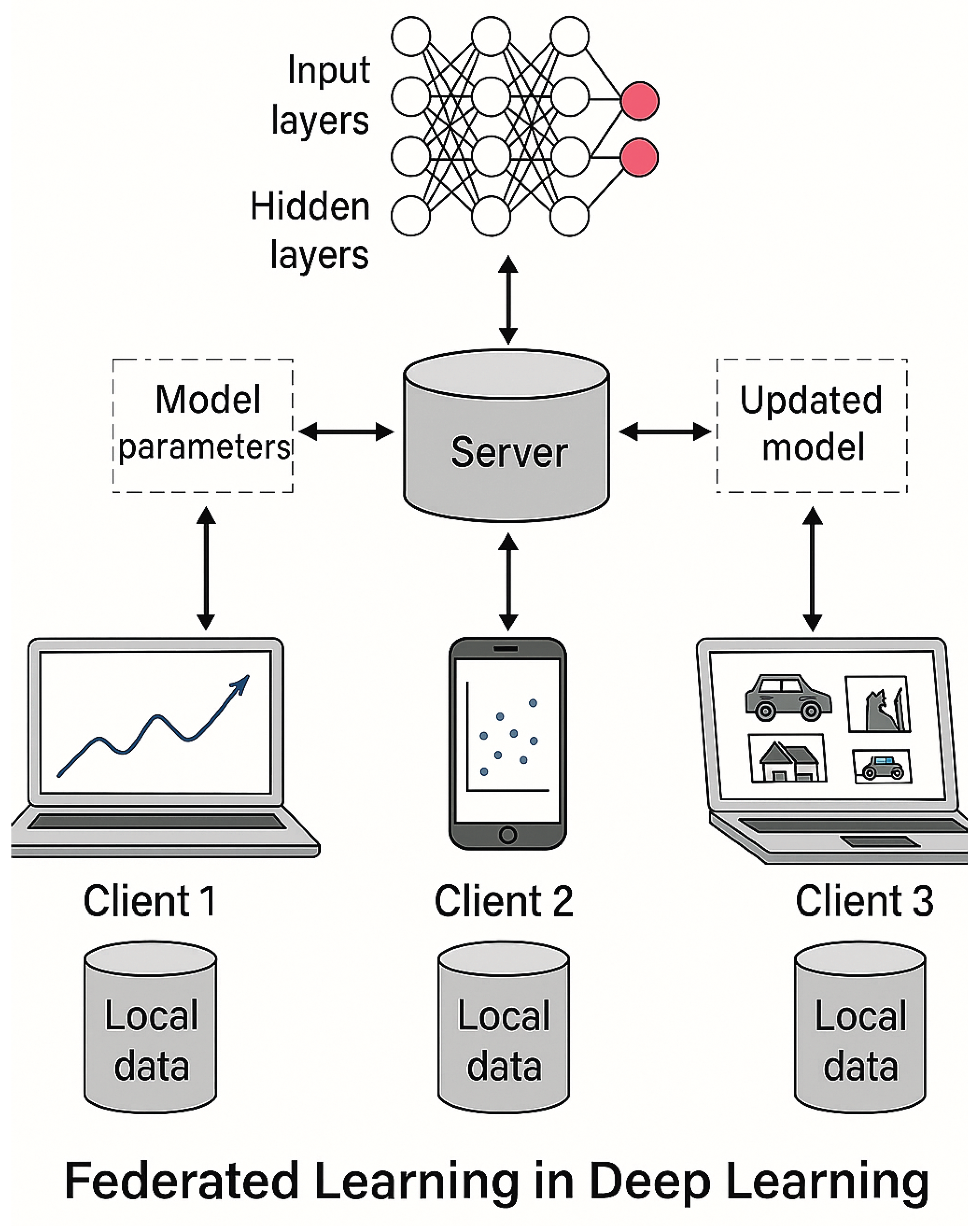
Federated learning (FL) is a decentralized machine learning paradigm where a global model is trained across multiple clients while keeping data localized, addressing privacy and data governance concerns. The framework involves K clients, each holding a local dataset drawn from a distribution , and a central server coordinating the training of a global model parameterized by . The objective is to minimize the global loss function:
where is the local loss for client k, ℓ is the per-sample loss function, and are aggregation weights satisfying . The canonical algorithm, Federated Averaging (FedAvg), iterates between local updates and global aggregation. In round t, the server broadcasts to a subset of clients . Each client performs local stochastic gradient descent (SGD) steps:
for , where is a mini-batch sample and is the learning rate. The server then aggregates the updates:
where the weights account for heterogeneous dataset sizes. Convergence analysis under non-IID data requires assumptions on gradient dissimilarity, quantified by the bounded variance condition:
for some . The convergence rate typically exhibits a dependence on and the number of communication rounds T, with optimal rates achieving under convexity and smoothness.
Differential privacy (DP) is often integrated into FL to provide formal privacy guarantees. Client-level DP ensures that participation of any single client does not significantly affect the model’s output. This is achieved by adding Gaussian noise to the aggregated updates:
where scales with the privacy budget . The privacy-utility trade-off is governed by the moments accountant method, which tracks the cumulative privacy loss across rounds. Byzantine robustness addresses malicious clients by replacing the averaging step with robust aggregation rules, such as coordinate-wise median or Krum:
which discards outliers. Theoretical guarantees for these methods rely on assumptions about the fraction of adversarial clients and the gradient distribution.
Personalized FL adapts the global model to individual clients by introducing local parameters or regularization. The objective becomes:
where are client-specific deviations and controls regularization. Model-agnostic meta-learning (MAML) variants optimize for fast adaptation:
where is the adaptation step size. These methods achieve convergence rates under strong convexity, with improvements in test accuracy on heterogeneous data. The interplay between communication efficiency, privacy, and personalization continues to drive theoretical and algorithmic advances in FL.
23.1. Literature Review of Federated Learning
The Literature Review of Federated Learning can be divided into 4 parts:
- Foundations of Federated Learning: The concept of Federated Learning was introduced by McMahan et al. (2017) [1186] in their seminal work, Communication-Efficient Learning of Deep Networks from Decentralized Data. They proposed Federated Averaging (FedAvg), an algorithm that allows distributed devices to train local models and share only the model updates instead of raw data. This work laid the foundation for privacy-preserving machine learning. Kairouz et al. (2021) [1187] provided a comprehensive survey on FL, covering its mathematical framework, privacy concerns, optimization techniques, and future research directions.
-
Privacy and Security in Federated Learning: One of the primary motivations for FL is preserving user privacy. Various studies have explored privacy-enhancing techniques, such as:
- –
- Differential Privacy (DP): Abadi et al. (2016) [1188] introduced differentially private SGD, which limits the influence of individual data points on model updates. This has been incorporated into FL to ensure user-level privacy.
- –
- Secure Aggregation: Bonawitz et al. (2017) [1189] developed cryptographic protocols to securely aggregate model updates, preventing adversaries from accessing individual updates.
- –
- Adversarial Attacks and Defenses: Zhao et al. (2018) [1190] studied model inversion attacks, highlighting the vulnerability of FL to privacy leakage and proposing defenses such as secure multi-party computation (MPC) and homomorphic encryption.
-
Communication Efficiency in Federated Learning: Efficient communication is crucial for FL due to the distributed nature of training. Several methods have been proposed to optimize communication:
- –
- Compression Techniques: Sattler et al. (2019) [1192] explored gradient compression techniques, such as quantization and sparsification, to reduce communication overhead.
- –
- Adaptive Federated Optimization: Reddi et al. (2020) [1193] proposed adaptive federated optimization methods, including FedProx and FedOpt, to enhance convergence and stability in heterogeneous data settings.
-
Personalization and Heterogeneous Data Handling: Unlike traditional centralized learning, FL operates on non-IID (independent and identically distributed) data across clients. Researchers have developed personalized FL approaches to address data heterogeneity:
- –
- Clustered FL: Sattler et al. (2020) [1194] introduced methods to group clients with similar data distributions for better model convergence.
- –
- Meta-Learning in FL: Fallah et al. (2020) applied meta-learning techniques in FL to improve model generalization across diverse clients.
-
Applications of Federated Learning: Federated Learning has been applied in various domains, including:
- –
- Healthcare: Sheller et al. (2020) [1196] demonstrated FL in medical imaging, allowing hospitals to collaboratively train models without sharing patient data.
- –
- Finance: Byrd and Polychroniadou et al. (2020) explored FL in fraud detection, improving prediction accuracy while ensuring data confidentiality.
- –
- Edge Computing: Jagatheesaperumal et al. (2021) [1198] studied FL for Internet of Things (IoT) applications, reducing reliance on cloud-based computation.
Despite its advantages, FL faces several challenges:
- Scalability: Efficient handling of a large number of clients remains an open research problem.
- Privacy-Utility Trade-off: Balancing privacy protection with model accuracy is an ongoing research area.
- Fairness and Bias: Addressing biases in FL models due to non-representative data distributions is a critical issue.
Federated Learning has revolutionized decentralized machine learning by enabling privacy-preserving collaborative model training. Significant progress has been made in improving security, communication efficiency, and personalization. However, challenges such as scalability, privacy-utility trade-offs, and fairness require further research.
23.2. Recent Literature Review of Federated Learning
Federated Learning (FL) has gained significant attention as a decentralized machine learning paradigm that allows multiple devices or institutions to collaboratively train models while keeping data localized, thus preserving privacy. Recent studies explore its applications, challenges, and optimizations across various domains, including healthcare, finance, cybersecurity, and IoT networks. Below is a comprehensive literature review highlighting key research in FL:
- Fundamentals and Privacy-Preserving Mechanisms in Federated Learning: Meduri et al. (2024) [1199] discuss a novel FL architecture for privacy-preserving analysis of electronic health records (EHRs), highlighting its benefits in rare disease research. The study introduces a secure communication framework that enhances data confidentiality in multi-institutional research. Tzortzis et al. (2025) [1200] explore generalizable FL in medical imaging, with a case study on mammography data. Their research compares centralized and decentralized training approaches, demonstrating that federated models can improve diagnosis accuracy while maintaining data sovereignty. Szelag et al. (2025) [1201] present a survey on adaptive adversaries in Byzantine-robust FL, discussing attacks on FL networks and countermeasures such as differential privacy, secure aggregation, and robust optimization strategies.
- Federated Learning for IoT and Smart Systems: Ferretti et al. (2025) [1203] propose a blockchain-based federated learning system for resilient and decentralized coordination, improving reliability and traceability in edge AI environments. Their approach ensures secure and tamper-proof federated model updates. Chen et al. (2025) [1204] introduce Federated Hyperdimensional Computing (FHC) for quality monitoring in smart manufacturing, which leverages hierarchical learning strategies to improve anomaly detection and predictive maintenance in industrial settings. Mei et al. (2025) [1205] explore semi-asynchronous FL control strategies in satellite networks, focusing on optimizing communication efficiency and reducing training latency in federated AI for space applications.
- Advances in Federated Learning for Edge AI and Security: Rawas and Samala (2025) [1206] introduce Edge-Assisted Federated Learning (EAFL) for real-time disease prediction, integrating FL with Edge AI to enhance processing efficiency while preserving patient data privacy. Becker et al. (2025) [1207] examine combined reconstruction and poisoning attacks on FL systems, assessing vulnerabilities and proposing mitigation strategies such as federated adversarial learning and model verification techniques.
- Optimization and Personalization in Federated Learning: Fu et al. (2025) present Personalized Federated Learning (Reads) [1208], incorporating fine-grained layer aggregation and decentralized clustering to address data heterogeneity among FL clients. Li et al. (2025) [1209] propose UltraFlwr, an efficient federated medical object detection framework designed to optimize federated model aggregation for medical imaging datasets. Shi et al. (2025) [1210] introduce FedLWS, a novel FL technique that applies layer-wise weight shrinking to improve training stability and reduce the risk of model overfitting.
- Federated Learning in Financial and Fraud Detection Applications: Choudhary (2025) [1212] reports on the integration of federated learning in fraud detection, demonstrating a 72 percentage reduction in privacy-related risks while maintaining high accuracy in financial anomaly detection. Zhou et al. (2025) [1213] introduce Blockchain-Empowered Cluster Distillation FL, which optimizes training efficiency in heterogeneous smart grids, ensuring robust energy management and fraud prevention.
Federated learning continues to evolve, addressing critical challenges such as communication overhead, security vulnerabilities, and model personalization. Future research is expected to focus on:
- Enhancing secure model aggregation using cryptographic techniques.
- Reducing computational costs for real-world FL deployment.
- Improving federated AI in healthcare, finance, and IoT by refining optimization algorithms.
This review highlights the latest advancements in FL, offering insights into its promising applications and the challenges that remain.
23.3. Formal Definition of Federated Learning
Federated Learning is a distributed optimization framework designed to solve the following empirical risk minimization (ERM) problem:
where represents the global model parameters, is the global objective function, is a probability distribution over clients, reflecting the heterogeneity of data distributions, is the local objective function for client k, defined as:
where is the local data distribution for client k, and is the loss function. Let M denote the global model, parameterized by , where d is the dimensionality of the model parameters. The goal is to minimize a global objective function , which is typically the average of local objective functions computed over the data held by each client k:
where K is the total number of clients, and is defined as:
Here, is the loss function (e.g., cross-entropy or mean squared error) evaluated on the data point , and is the number of data points on client k.
23.4. Federated Learning and Distributed Optimization Framework
Federated Learning operates in a distributed setting with K clients and a central server. The optimization process can be formalized as follows:
23.4.1. Clients
In Federated Learning, clients are the distributed entities (e.g., mobile devices, IoT devices, or institutional servers) that hold local datasets , where indexes the clients. Each client k participates in the collaborative training of a global model M, parameterized by , without sharing its raw data . Each client k maintains a local dataset and computes updates to the global model parameters w based on its local data. Each client k is associated with a local objective function , which represents the expected loss over its local data distribution :
where:
- is the loss function (e.g., cross-entropy, mean squared error) evaluated on a data point .
- is the local dataset of client k, which may differ significantly from other clients’ datasets (non-IID data).
Clients are responsible for computing updates to the global model parameters w based on their local data. This process typically involves local stochastic gradient descent (SGD) or its variants. The local update rule at communication round t is:
where is the learning rate at round t and is the stochastic gradient computed on a mini-batch . Clients can also train personalized models that adapt to their local data distribution . This can be achieved by adding a regularization term to the local objective function:
where controls the degree of personalization. Clients can ensure privacy by adding noise to their local updates:
where is calibrated to achieve -differential privacy. To reduce communication costs, clients can transmit only a subset of the model parameters:
Clients in FL face several challenges, which are rigorously described below:
- Non-IID Data: The local data distribution may differ significantly from the global data distribution D, leading to statistical heterogeneity. This can be quantified by the gradient divergence:where measures the degree of non-IIDness.
- Resource Constraints: Clients often have limited computational resources (e.g., CPU, memory) and communication bandwidth. This necessitates efficient algorithms for local training and model compression.
- Privacy and Security: Clients must ensure that their local data is not exposed during training. Techniques such as differential privacy and secure multi-party computation (SMPC) are employed to protect client data.
23.4.2. Server
A central server orchestrates the training process by aggregating the local updates from the clients and updating the global model. The most common aggregation method is Federated Averaging (FedAvg), which computes a weighted average of the local model parameters:
where
is the total number of data points across all clients. The server can use adaptive aggregation methods to account for heterogeneous client updates. For example, weighted aggregation assigns higher weights to clients with larger datasets or more reliable updates:
where is the weight assigned to client k. To ensure privacy, the server can use secure multi-party computation (SMPC) to aggregate client updates without revealing individual contributions:
The server can add noise to the global model updates to ensure differential privacy:
The server in FL faces several challenges, which are described below:
- Heterogeneous Client Participation: Clients may have varying computational resources, communication bandwidth, and availability, leading to asynchronous participation. The server must handle this heterogeneity to ensure efficient training.
- Non-IID Data: The local data distributions may differ significantly across clients, leading to statistical heterogeneity. This can cause client drift and slow convergence. The server must account for this by using robust aggregation methods.
- Privacy and Security: The server must ensure that the global model updates do not leak sensitive information about the clients’ local data. Techniques such as secure aggregation and differential privacy are employed to protect client privacy.
23.4.3. Local Updates
Each client k performs stochastic gradient descent (SGD) on its local objective function . The local update rule at iteration t is:
where is the learning rate at iteration t, is the stochastic gradient computed on a mini-batch . In Federated Learning, the local model update at each client node constitutes a fundamental component of the distributed optimization process. Specifically, each client seeks to minimize its own local objective function , which is typically defined as the empirical risk over its local dataset . Mathematically, this local objective can be expressed as
where denotes the individual loss incurred on data sample i belonging to client k. The global objective function over all participating clients can then be written as a weighted sum of the local objectives:
where represents the relative contribution (or participation weight) of client k based on its local dataset size.
During each communication round t, client k performs local stochastic gradient descent (SGD) updates to minimize . The update rule for client k at local iteration t is given by
where is the learning rate (step size) at iteration t, and denotes the stochastic gradient computed over a mini-batch . Explicitly, this stochastic gradient can be expanded as
The stochasticity arises due to the random sampling of the mini-batch , implying that
which ensures that the stochastic gradient is an unbiased estimator of the true gradient. The variance of this estimator can be characterized as
and under bounded variance assumptions, one typically has
where quantifies the degree of stochastic noise in the gradient estimation process. Expanding the update rule recursively over local iterations yields
which shows how each client independently evolves its local model parameters based on the trajectory of locally computed stochastic gradients. Assuming the loss function is L-smooth, the gradient satisfies
which allows bounding the deviation of local updates from the global optimum and contributes to convergence rate analysis. Additionally, the expected decrease in the local objective function value per iteration can be rigorously expressed as
demonstrating the fundamental trade-off between the learning rate, smoothness of the objective, and the variance of stochastic gradients.
Finally, after completing the local optimization phase, each client transmits its locally updated model back to the central server, which subsequently performs the aggregation step as
thus combining the contributions of all participating clients in a manner that reflects the relative statistical importance of their respective datasets. This process tightly couples the local SGD dynamics at each client with the global update mechanism of the federated system, ensuring a coherent evolution of the global model parameters through iterative decentralized learning.
23.4.4. Model Aggregation
The server aggregates the local updates using a weighted average:
where is the weight assigned to client k, typically proportional to the size of its local dataset . We consider K clients indexed by . Let denote the local dataset of client k with cardinality and total sample size . Define the local empirical risk and the global (data-proportional) empirical risk by
where is the per-sample loss (assumed differentiable when needed). Let the server-assigned weights be with ; the canonical choice is . The server aggregates local models into the global model by the convex combination
The aggregation is the unique minimizer of the weighted least-squares objective
Indeed,
and is strictly convex whenever some , hence the minimizer is unique. From convexity we have, for any ,
Assume each is L-smooth, i.e. for all , we have
Assume stochastic gradients on client k are unbiased conditional estimators of the true local gradient: for any appropriate local iterate ,
and denote the conditional covariance by . If every client performs a single exact full-batch gradient step from the common server model ,
then the aggregated update equals the centralized gradient descent step on F:
Thus, under one synchronized exact gradient step per client and , federated aggregation reproduces centralized gradient descent on the global empirical objective F.
Consider the practical FedAvg local-SGD update where each client k starts from and performs local stochastic-gradient steps with step-size . Let denote the stochastic gradient at local step on client k. Then
Aggregation yields
Taking conditional expectation given history and using unbiasedness,
Define the aggregated stochastic increment . Under independence of client noise, the conditional covariance of satisfies
If for each client-step we have the variance bound and steps are uncorrelated within a client (or conservatively bounded), then (scalar variance upper bound)
Thus variance of the aggregated update scales with , illustrating that larger-weight clients contribute quadratically via to the aggregated variance.
The deviation (bias) of the expected aggregated update from the ideal centralized multi-step descent direction can be bounded under (L)-smoothness and a gradient-norm bound . We have
Using L-smoothness and the telescoping bound
we obtain
and therefore
Summing over clients with weights yields the bias bound
Thus the local-drift bias scales on the order of (for large ), quantifying how multiple local steps cause the aggregated expected direction to deviate from the centralized .
Apply the smoothness (descent) lemma for F with L-smoothness: for any w and ,
Set and . Taking conditional expectation and using unbiasedness,
Decompose the inner product as
so the drift term subtracts from the ideal descent and must be controlled by small and/or small to guarantee net expected decrease in F. The squared-norm term satisfies
Using the variance decomposition and the bound gives explicit control of the stochastic term and shows how governs the noise amplitude.
Alternative weighting choices introduce explicit trade-offs. The canonical data-proportional weight
aligns the federated objective with the global empirical risk F and yields the unbiased equivalence to centralized gradient descent when local steps are synchronized single-batch gradients. Uniform weighting enforces equal client influence (fairness) but no longer makes F equal the sample-average empirical risk; reliability-weighting with adjusts influence by a trust or availability score; adaptive importance weighting may take the form
with normalization , trading statistical optimality for fairness or robustness.
A small numerical illustration: let , , so and . If and , then
which lies in the convex hull of the client models and is biased toward the larger client. More generally, for any two vectors and weight ,
Collecting the algebraic identities and bounds, the aggregation rule satisfies
and the bias from centralized multi-step descent obeys
Consequently, choices of , , and jointly determine the bias–variance trade-off: data-proportional minimizes mismatch with the empirical global objective, while small or small control local-drift bias and variance to permit descent according to the smoothness lemma
with the explicit drift and variance terms given above. These equalities and inequalities provide a precise, equation-rich characterization of model aggregation in federated learning, explicating the algebraic, statistical, and optimization-theoretic consequences of the weighted-average rule .
23.5. Detailed Steps in a Communication Round
Federated Learning proceeds iteratively in communication rounds. In each round t:
- Client Selection: At the start of each communication round t, the server selects a subset of clients to participate. The selection may be random or based on criteria such as client availability, computational resources, or data distribution. The probability of selecting client k is denoted by , where
- Model Distribution: The server sends the current global model parameters to the selected clients .
- Local Training: Each selected client performs steps of local stochastic gradient descent (SGD) on its dataset to compute updated parameters . The local update rule at local step s is:where is the learning rate at round t, is the stochastic gradient computed on a mini-batch . After steps, the client sends the updated parametersback to the server.
- Model Aggregation: The server aggregates the local updates from the selected clients using Federated Averaging (FedAvg):where is the number of data points on client k and is the total number of data points across the selected clients.
23.5.1. Challenges in Communication Rounds
Communication rounds in FL face several challenges, which are rigorously described below:
- Heterogeneous Client Participation: Clients may have varying computational resources, communication bandwidth, and availability, leading to asynchronous participation. This can slow down the training process and introduce bias in the model updates.
- Non-IID Data: The local data distributions may differ significantly across clients, leading to statistical heterogeneity. This can cause client drift and slow convergence.
- Communication Bottlenecks: The communication between the server and clients can be a bottleneck, especially in large-scale FL systems with millions of clients. Techniques such as model compression and sparse updates are used to reduce communication costs.
23.5.1.1 Heterogeneous Client Participation
In Federated Learning, heterogeneous client participation refers to the scenario where clients exhibit significant variability in their participation patterns, computational resources, and data distributions. Specifically, clients may differ in their participation probabilities, computational resources, and data distributions, leading to asynchronous updates and biased model aggregation. These forms of heterogeneity slow down convergence and degrade the performance of the global model. To rigorously analyze these effects, we begin by defining the global objective function , which is the average of the local objective functions computed over the data held by each client k. The global objective function is given by:
where represents the global model parameters, and is the local objective function for client k, defined as:
Here, is the loss function evaluated on a data point , and is the local dataset of client k.
Heterogeneous client participation arises when the participation probabilities vary significantly across clients, and the local data distributions are non-IID. The global model update at round t is given by:
where denotes the subset of clients participating in communication round t, is the number of data points on client k, and is the total number of data points across the selected clients. Taking the expectation over client participation, the expected global model update is:
where is the total number of data points across all clients. If is not uniform, the expected update is biased toward clients with higher . This bias can be quantified as:
Heterogeneous client participation slows down convergence due to the increased variance in model updates and the reduced effective learning rate.
The variance of the global model updates increases because clients contribute unevenly to the training process. Specifically, the variance of the global update is given by:
When clients participate heterogeneously, the variance term becomes larger, which slows down convergence. The effective learning rate is reduced because the global model update is dominated by a subset of clients. This can be seen by analyzing the expected update direction:
If is not uniform, the update direction is biased toward the gradients of frequently participating clients, reducing the effective step size. Heterogeneous client participation also introduces bias in the model updates due to non-IID data distributions. When clients have non-IID data, the local objective functions differ significantly. If clients participate heterogeneously, the global model update is biased toward the local objectives of more frequently participating clients. This bias can be quantified as:
The bias introduced by heterogeneous participation degrades model performance because the global model overfits to the data of frequently participating clients and underfits to the data of rarely participating clients. To rigorously analyze the impact of heterogeneous participation on convergence, we consider the expected suboptimality gap , where is the optimal solution. The expected suboptimality gap evolves according to the following recurrence relation:
where is the strong convexity parameter, L is the smoothness parameter, is the variance of the stochastic gradients, and is the squared bias due to heterogeneous participation.
For a constant learning rate , the recurrence relation can be solved as:
To achieve , we require:
This shows that the number of communication rounds T increases due to the bias term . The bias in gradient estimation arises because the global gradient is estimated as:
If is not uniform, the gradient estimate is biased toward the gradients of frequently participating clients. This bias can be quantified as:
The biased gradient estimate slows down convergence because the global model update direction is no longer aligned with the true gradient , and the effective step size is reduced due to the bias. In conclusion, heterogeneous client participation slows down the training process and introduces bias in the model updates due to the uneven contribution of clients to the global model update and the non-IID data distributions across clients. These effects are rigorously quantified using tools from optimization theory and statistical learning. By addressing heterogeneous participation, we can improve the convergence and performance of Federated Learning.
23.5.1.2 Communication Bottlenecks
In Federated Learning, communication bottlenecks refer to the limitations imposed by the communication infrastructure between the server and the clients. These bottlenecks arise due to limited bandwidth, high latency, and frequent communication, which slow down the training process and increase the overall time required to achieve convergence. To rigorously analyze these effects, we begin by defining the global objective function , which is the average of the local objective functions computed over the data held by each client k. The global objective function is given by:
where represents the global model parameters, and is the local objective function for client k, defined as:
Here, is the loss function evaluated on a data point , and is the local dataset of client k. Communication bottlenecks affect both the downlink (server to clients) and uplink (clients to server) transmissions. The time required for downlink communication is given by:
where d is the dimensionality of the model parameters, b is the number of bits used to represent each parameter, and is the downlink bandwidth. The time required for uplink communication is given by:
where is the uplink bandwidth. The total time required for each communication round t is given by:
where is the time required for local computation on the clients.
Communication bottlenecks increase and , thereby increasing and slowing down the overall training process. The effective learning rate is reduced because the global model is updated less frequently. The effective learning rate is given by:
where is the nominal learning rate. A smaller slows down convergence. Communication bottlenecks also increase the variance of the global model updates because clients may not be able to transmit their updates in a timely manner. This variance can be quantified as:
To rigorously analyze the impact of communication bottlenecks on convergence, we consider the expected suboptimality gap , where is the optimal solution. The expected suboptimality gap evolves according to the following recurrence relation:
where is the strong convexity parameter, L is the smoothness parameter, is the variance of the stochastic gradients, and is the variance of the global model updates due to communication bottlenecks.
For a constant effective learning rate , the recurrence relation can be solved as:
To achieve , we require:
This shows that the number of communication rounds T increases due to the reduced effective learning rate and the increased variance . To mitigate the impact of communication bottlenecks, several techniques can be employed. Model compression techniques, such as quantization and sparsification, reduce the number of bits b required to represent each parameter. This reduces the communication time and . Clients can perform multiple local updates before communicating with the server. This reduces the frequency of communication and increases the effective learning rate . Asynchronous updates allow clients to communicate with the server at different times, reducing the impact of high latency. In conclusion, communication bottlenecks slow down the training process and increase the overall time required to achieve convergence in Federated Learning. These effects are rigorously quantified using tools from optimization theory, information theory, and statistical learning. By addressing communication bottlenecks, we can improve the efficiency and performance of Federated Learning.
23.5.1.3 Non-IID Data
In Federated Learning, statistical heterogeneity refers to the scenario where the local data distributions differ significantly across clients. This heterogeneity arises due to differences in the data generation processes, user behaviors, or environmental factors across clients. Statistical heterogeneity can lead to client drift, where the local models trained on different clients diverge from the global model, and slow convergence, where the global model takes longer to reach the optimal solution. To rigorously analyze these effects, we begin by defining the global objective function , which is the average of the local objective functions computed over the data held by each client k. The global objective function is given by:
where represents the global model parameters, and is the local objective function for client k, defined as:
Here, is the loss function evaluated on a data point , and is the local dataset of client k.
Statistical heterogeneity arises when the local data distributions differ significantly from the global data distribution , which can be quantified using measures such as the total variation distance or the Kullback-Leibler (KL) divergence. For example, the total variation distance between and is given by:
When is large, the local data distribution is significantly different from the global data distribution .
Statistical heterogeneity affects the local objective functions , which are defined as:
When differs significantly from , the local objective functions differ significantly from the global objective function , which is defined as:
This difference can be quantified using the gradient divergence:
where measures the degree of statistical heterogeneity. Client drift occurs when the local models trained on different clients diverge from the global model due to statistical heterogeneity. This can be rigorously analyzed using the local update rule:
where is the learning rate at round t, and is the stochastic gradient computed on a mini-batch . When differs significantly from , the local updates diverge from the global update direction . This divergence can be quantified as:
When is large, the divergence becomes large, leading to client drift. Statistical heterogeneity slows down convergence because the global model update direction is no longer aligned with the true gradient . This can be rigorously analyzed using the expected suboptimality gap , where is the optimal solution. The expected suboptimality gap evolves according to the following recurrence relation:
where is the strong convexity parameter, L is the smoothness parameter, is the variance of the stochastic gradients, and is the gradient divergence due to statistical heterogeneity. For a constant learning rate , the recurrence relation can be solved as:
To achieve , we require:
This shows that the number of communication rounds T increases due to the gradient divergence . To mitigate the impact of statistical heterogeneity, several techniques can be employed. Regularization can be added to the local objective function to reduce the divergence between local and global models.
Personalized Federated Learning can be used to train personalized models for each client that adapt to their local data distributions. Data augmentation can be used to augment the local data to make the local data distributions more similar to the global data distribution. In conclusion, statistical heterogeneity, where the local data distributions differ significantly across clients, leads to client drift and slow convergence in Federated Learning. These effects are rigorously quantified using tools from optimization theory, probability theory, and statistical learning. By addressing statistical heterogeneity, we can improve the convergence and performance of Federated Learning.
23.5.1.4 Python Code to Generate Figure 211, Figure 212, and Figure 213 Illustrating Heterogeneous Client Participation in Federated Learning
The Python code below produces the Figure 211, Figure 212, and Figure 213 illustrating Heterogeneous Client Participation in federated learning.
Figure 211.
Heterogeneous client participation in federated learning over rounds. Each row corresponds to a client and each column to a communication round; a dark cell indicates the client participated in that round
Figure 211.
Heterogeneous client participation in federated learning over rounds. Each row corresponds to a client and each column to a communication round; a dark cell indicates the client participated in that round
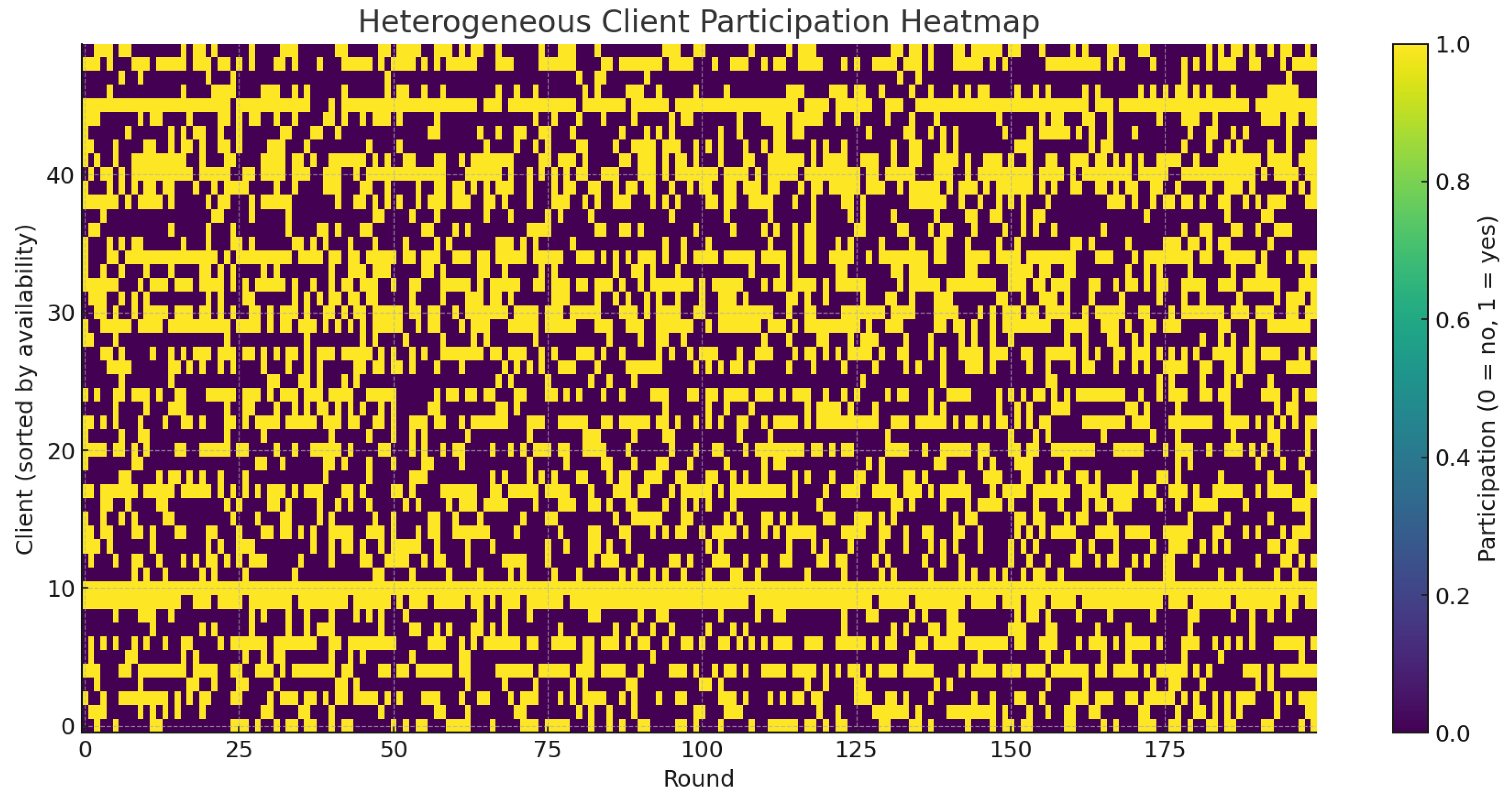
Figure 212.
Number of clients participating in each federated learning round. The line shows how client participation varies across rounds under heterogeneous availability
Figure 212.
Number of clients participating in each federated learning round. The line shows how client participation varies across rounds under heterogeneous availability
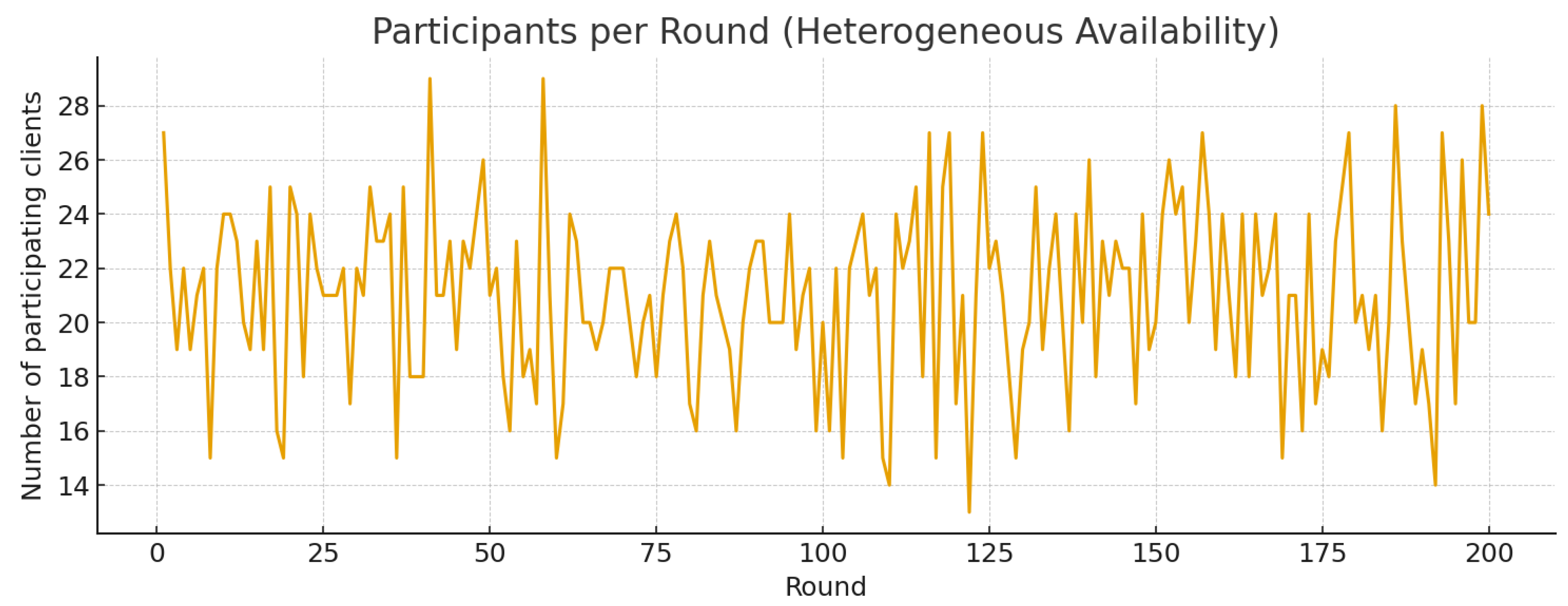
Figure 213.
Total participation frequency per client, sorted from most to least active. This highlights heterogeneity in client involvement
Figure 213.
Total participation frequency per client, sorted from most to least active. This highlights heterogeneity in client involvement
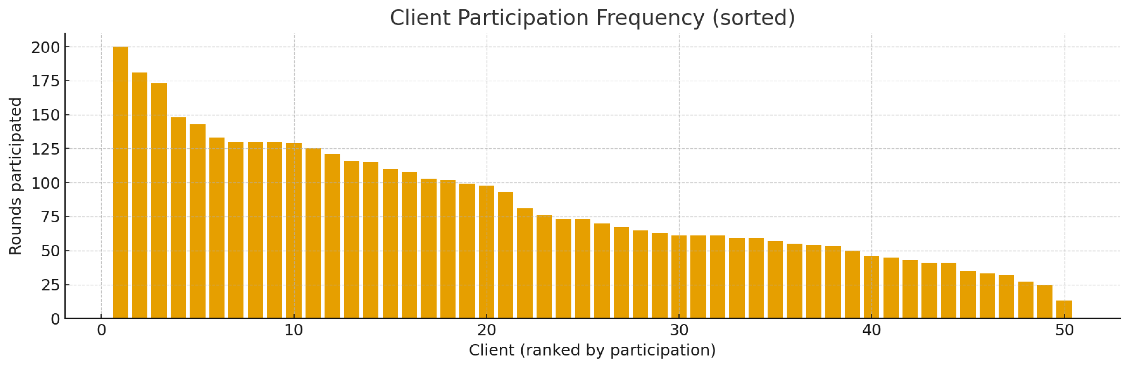
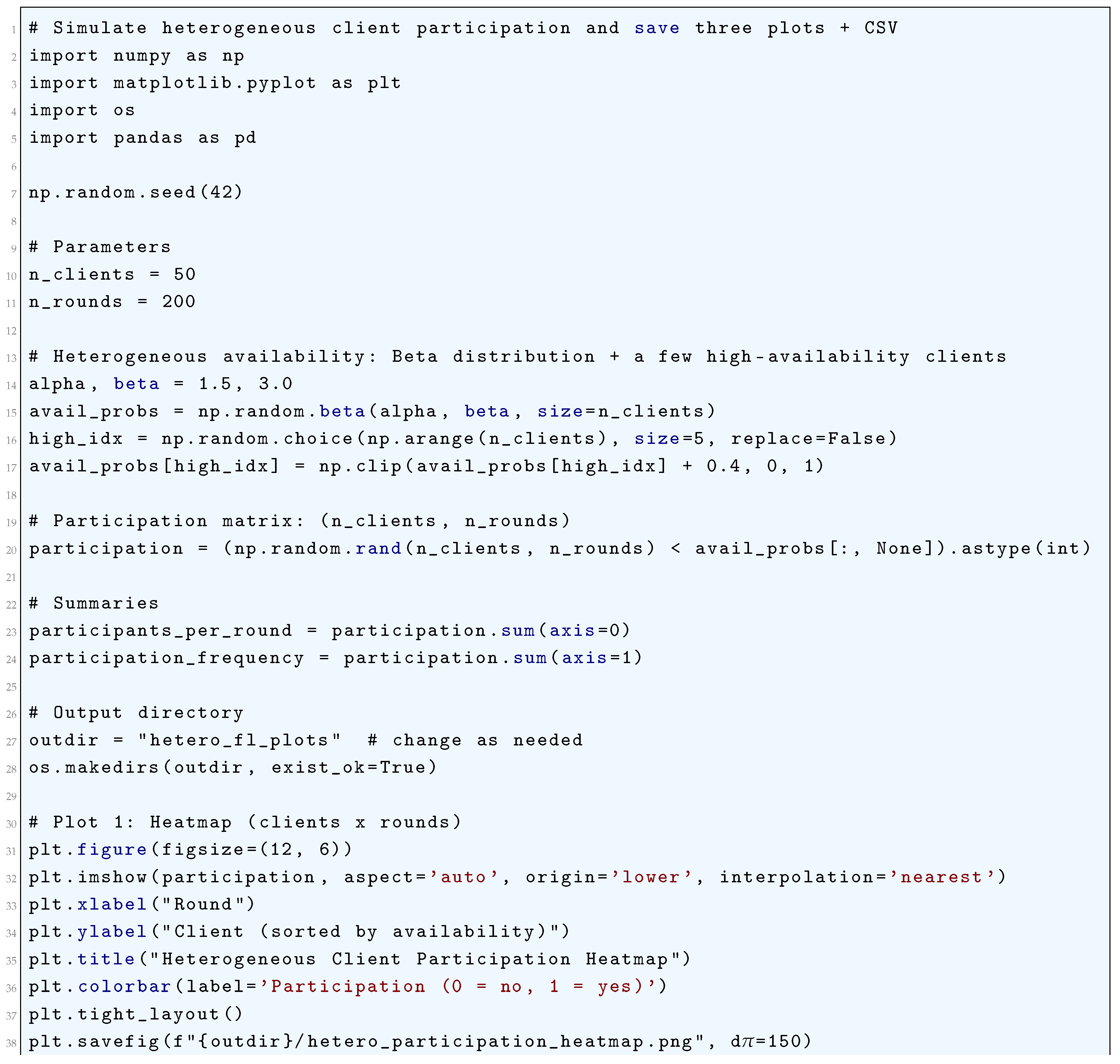
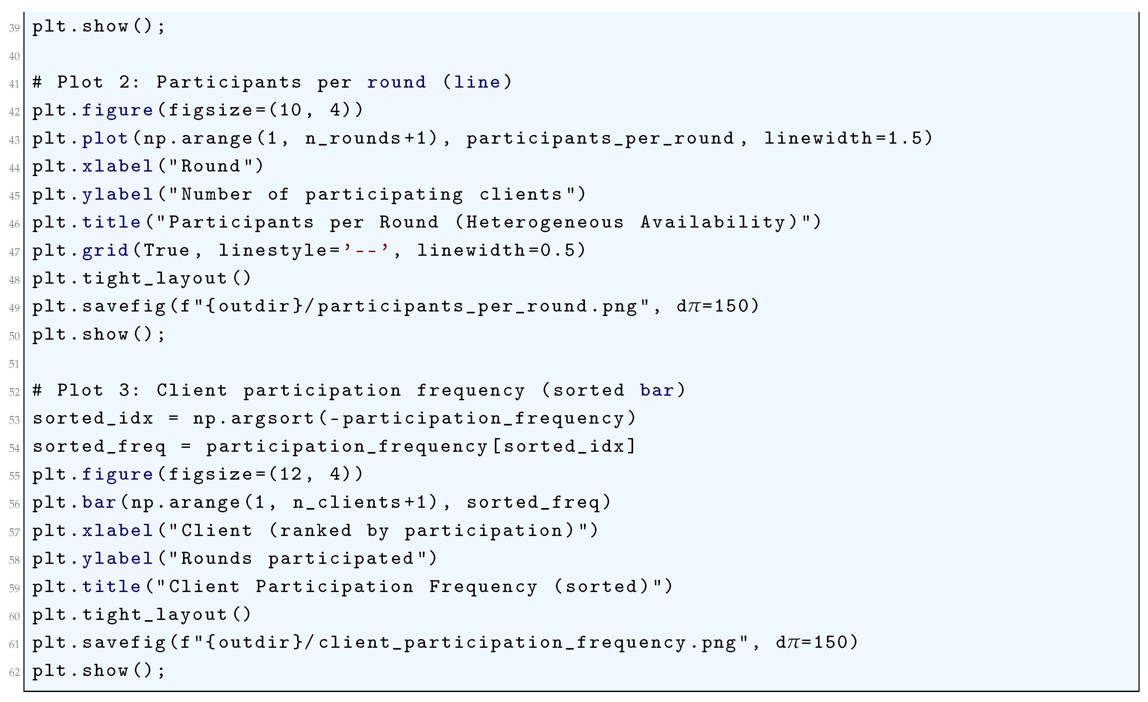
23.5.1.5 Python Code to Generate Figure 214 and Figure 215 Illustrating Communication Bottlenecks and Cumulative Communication over Rounds in Federated Learning
The Python code below produces the Figure 214 and Figure 215 illustrating Communication Bottlenecks and Cumulative communication over rounds in federated learning.
Figure 214.
Total and average client communication per round in federated learning. Dashed line shows average communication per client, while the solid line shows total communication, highlighting potential bottlenecks due to client heterogeneity
Figure 214.
Total and average client communication per round in federated learning. Dashed line shows average communication per client, while the solid line shows total communication, highlighting potential bottlenecks due to client heterogeneity
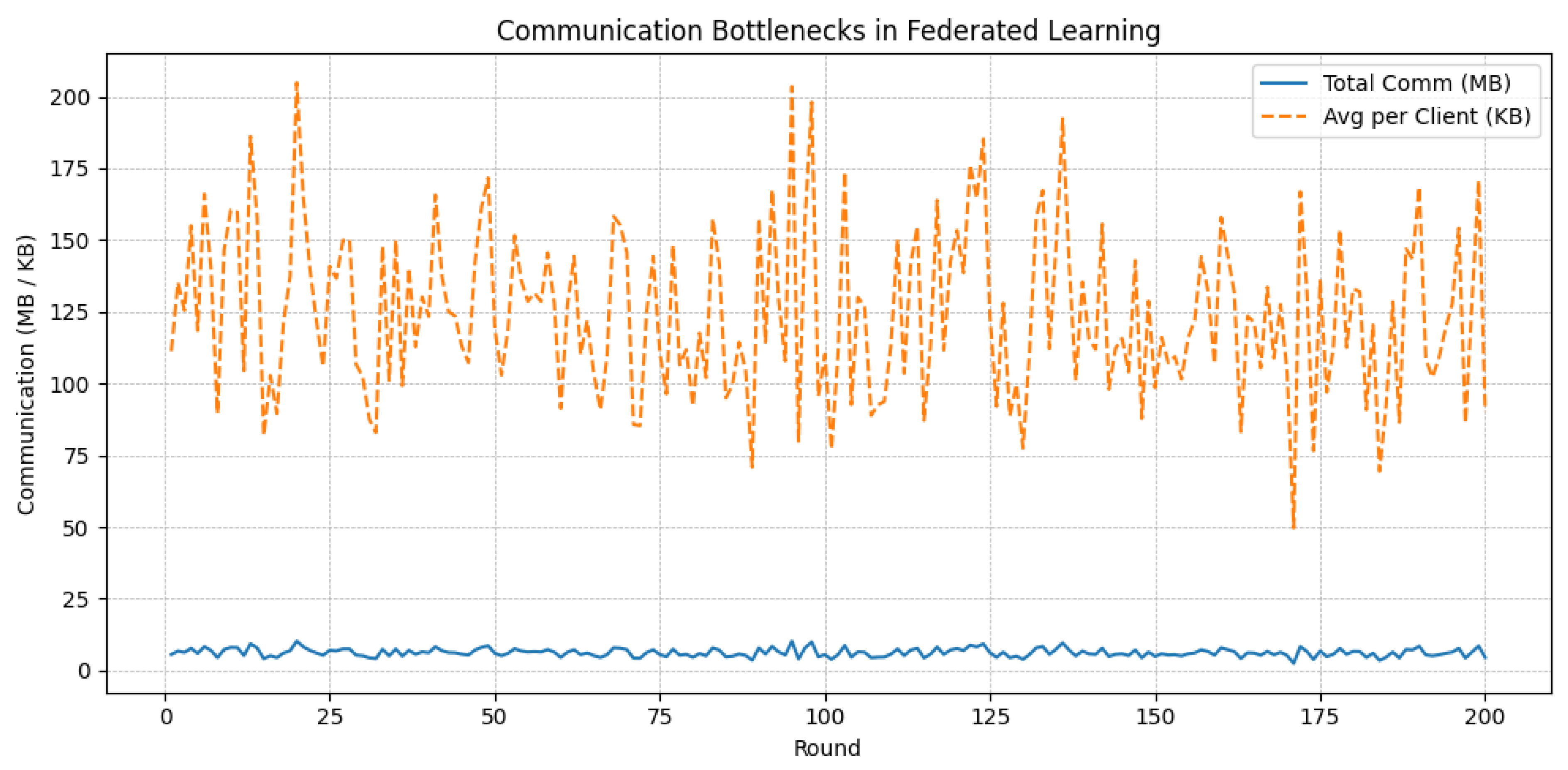
Figure 215.
Cumulative communication over rounds in federated learning. The slope shows aggregate communication growth, indicating long-term bandwidth demands and bottlenecks
Figure 215.
Cumulative communication over rounds in federated learning. The slope shows aggregate communication growth, indicating long-term bandwidth demands and bottlenecks
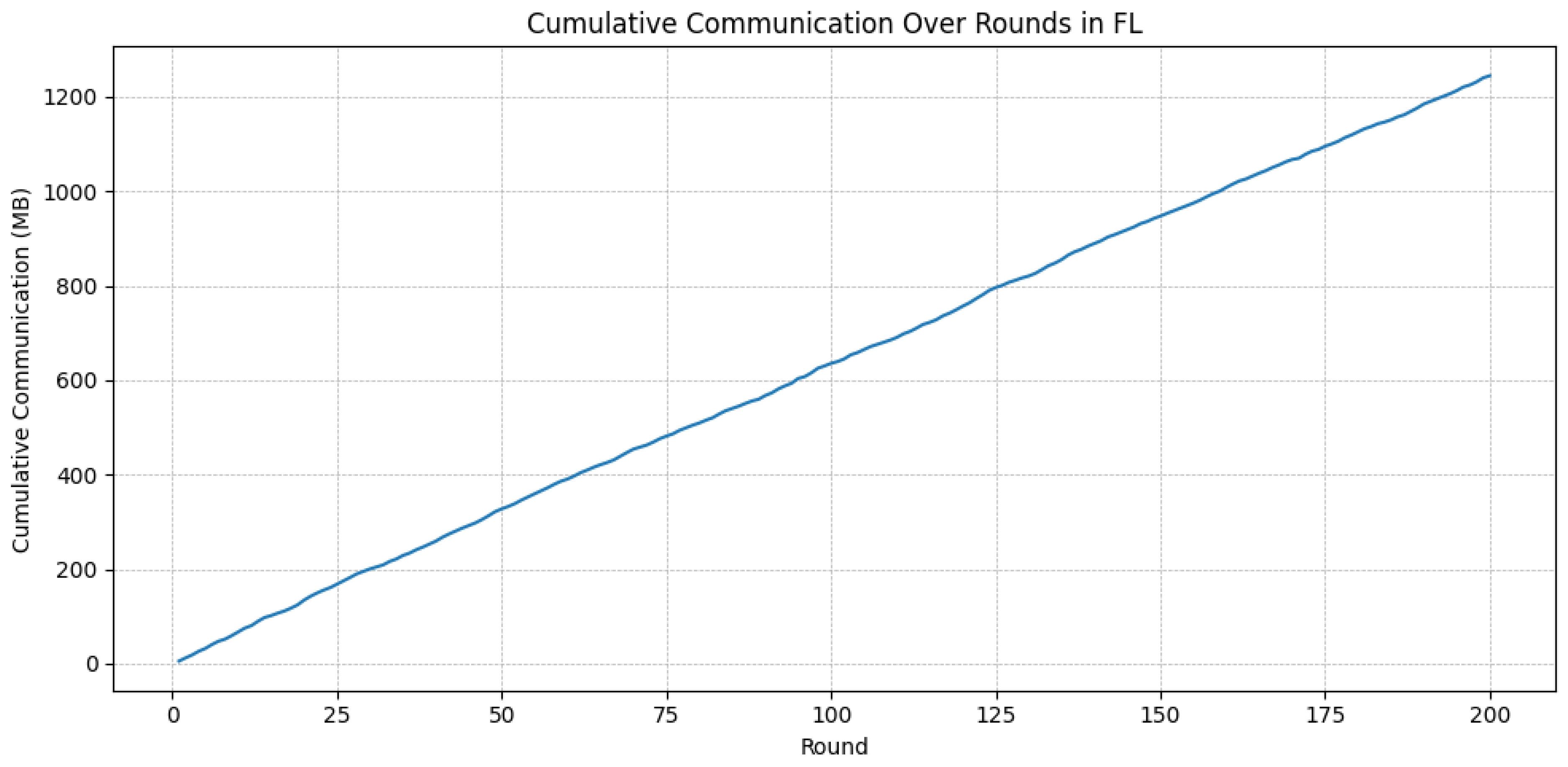
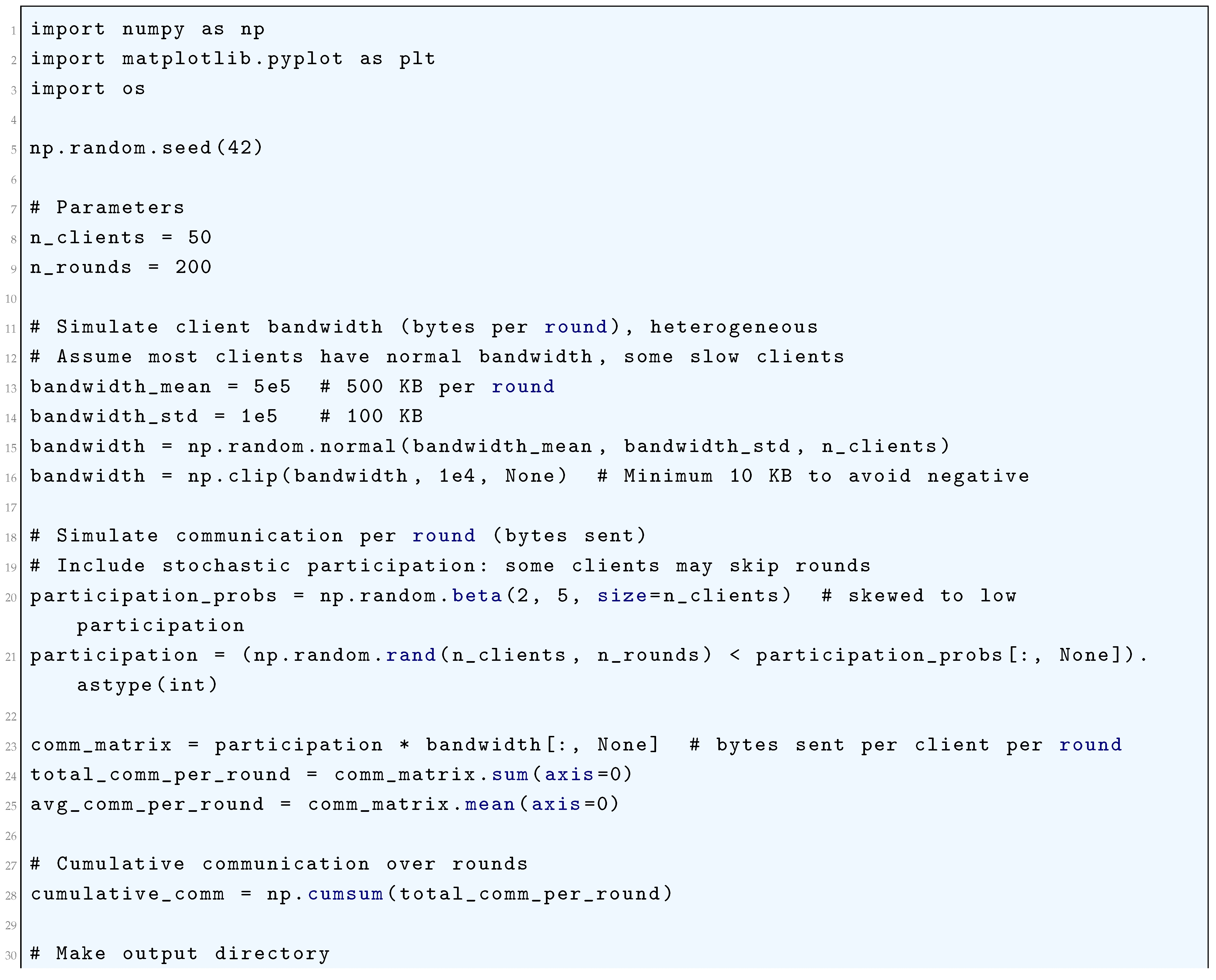
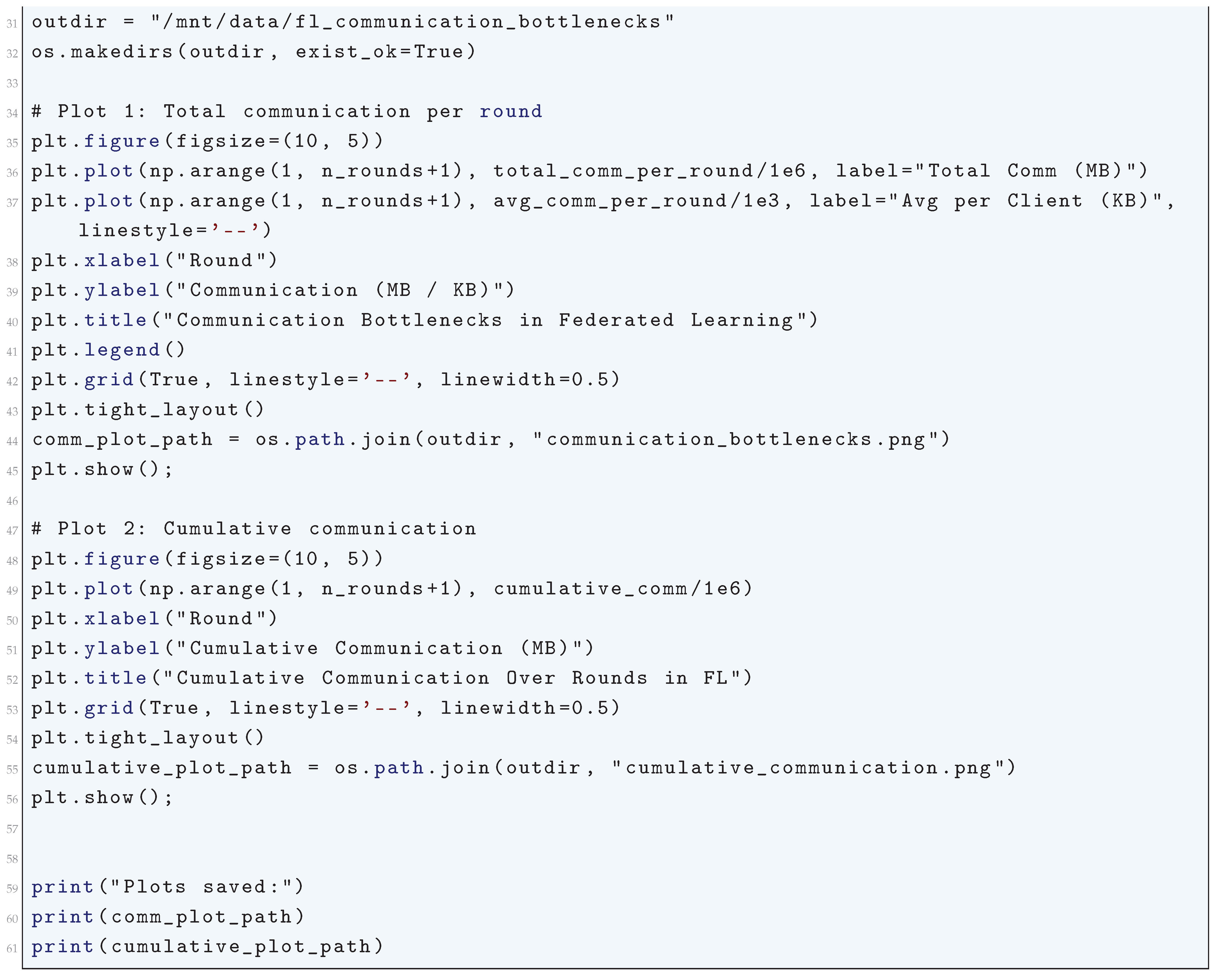
23.5.1.6 Python Code to Generate Figure 216 Illustrating Client Drift in Federated Learning, Measured as L2 Distance from the Global Model
The Python code below produces the Figure 216 illustrating Client drift in federated learning, measured as L2 distance from the global model.
Figure 216.
Client drift in federated learning, measured as L2 distance from the global model. Each colored line represents an individual client, and the black bold line shows the average drift across all clients. Client drift arises due to heterogeneity in local updates and data distribution
Figure 216.
Client drift in federated learning, measured as L2 distance from the global model. Each colored line represents an individual client, and the black bold line shows the average drift across all clients. Client drift arises due to heterogeneity in local updates and data distribution
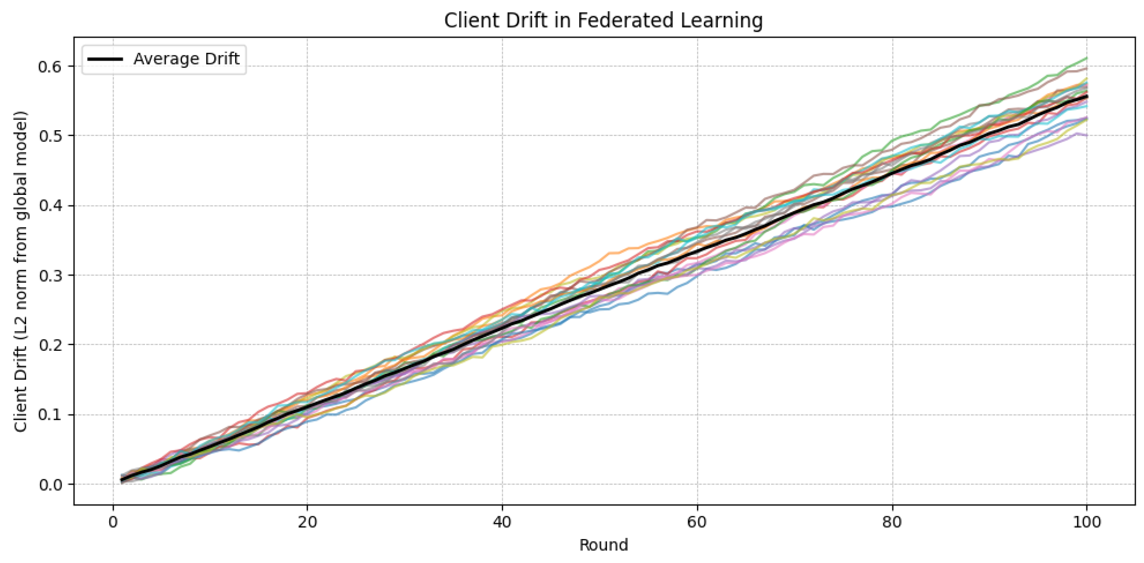
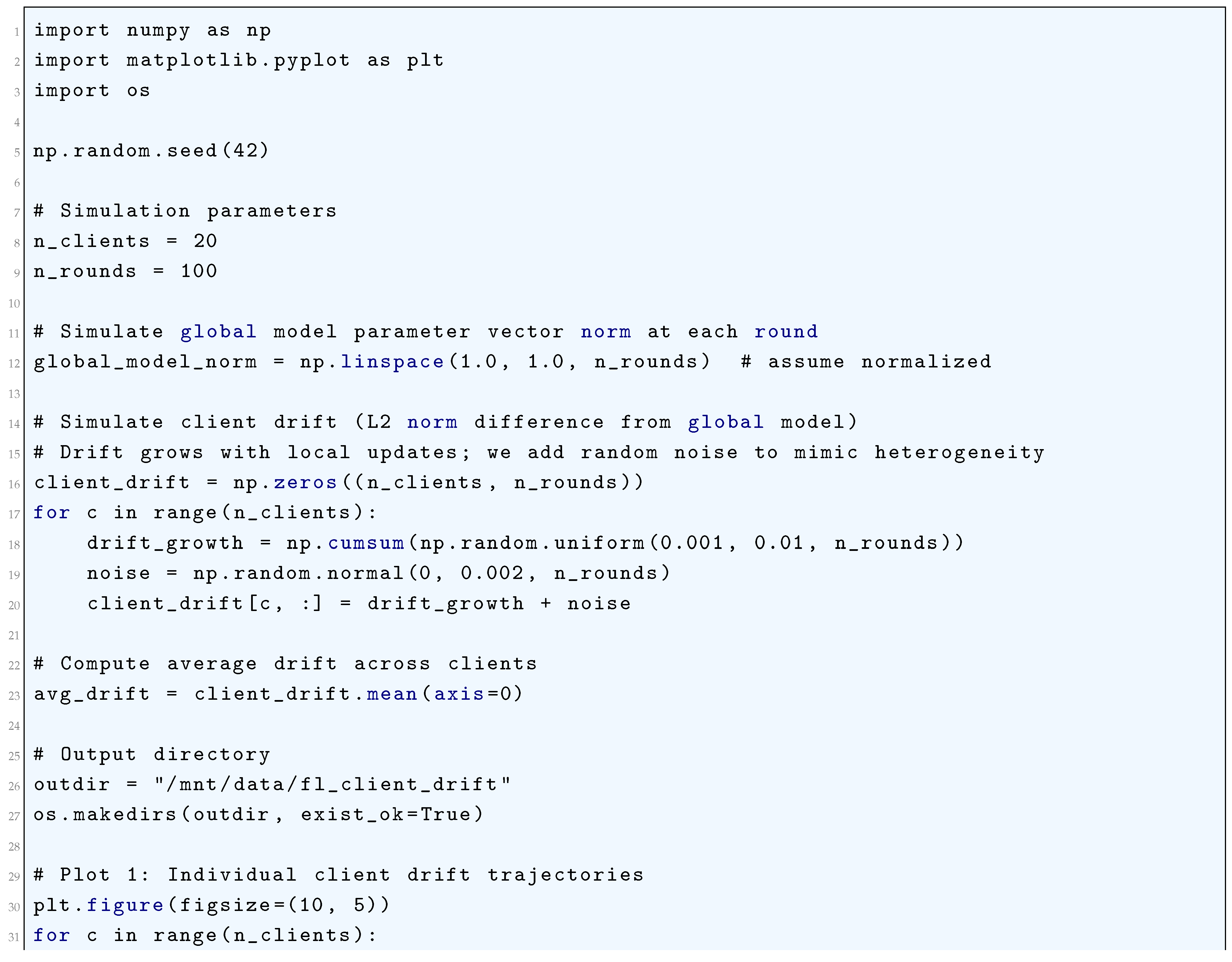
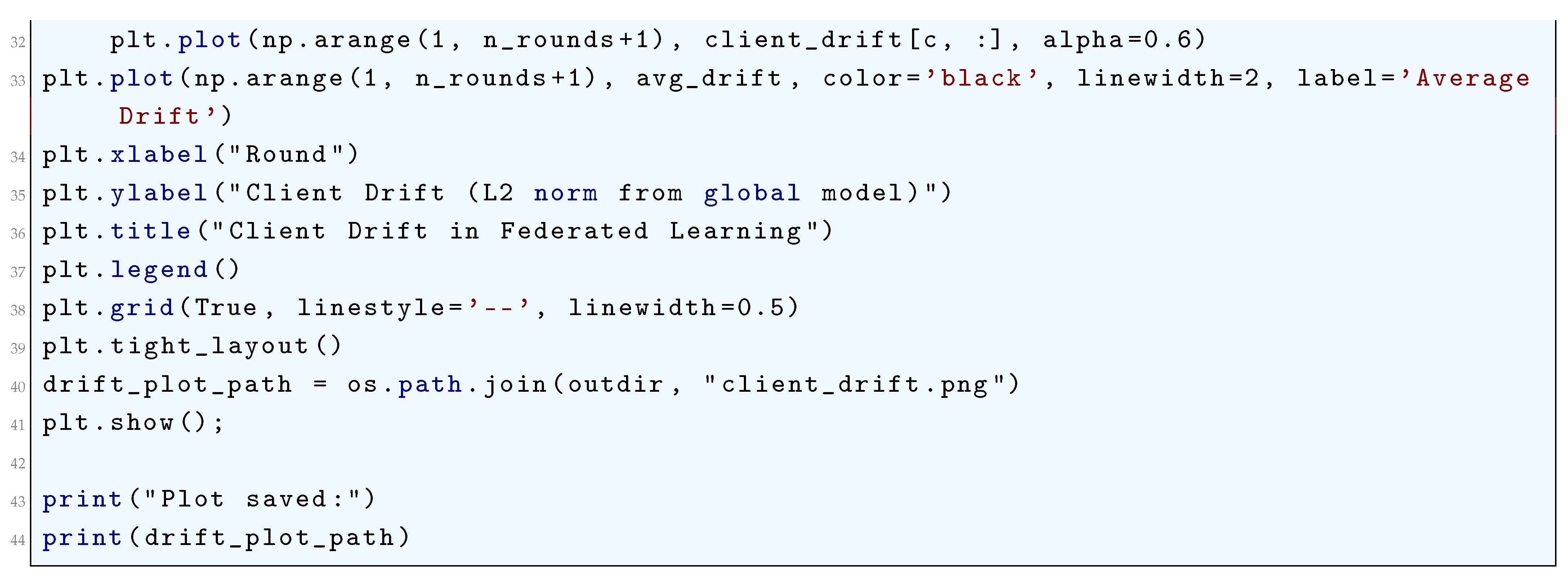
23.5.1.7 Python Code to Generate Figure 217 Illustrating Comparative Client Drift Under Different Heterogeneity Scenarios in Federated Learning
The Python code below produces the Figure 217 illustrating Comparative client drift under different heterogeneity scenarios in federated learning.
Figure 217.
Comparative client drift under different heterogeneity scenarios in federated learning. Each transparent line represents an individual client, and the bold lines show the average drift for each scenario: green: IID, orange: Mild Non-IID, red: Highly Non-IID. Greater drift occurs for highly non-iid data due to divergence in local updates
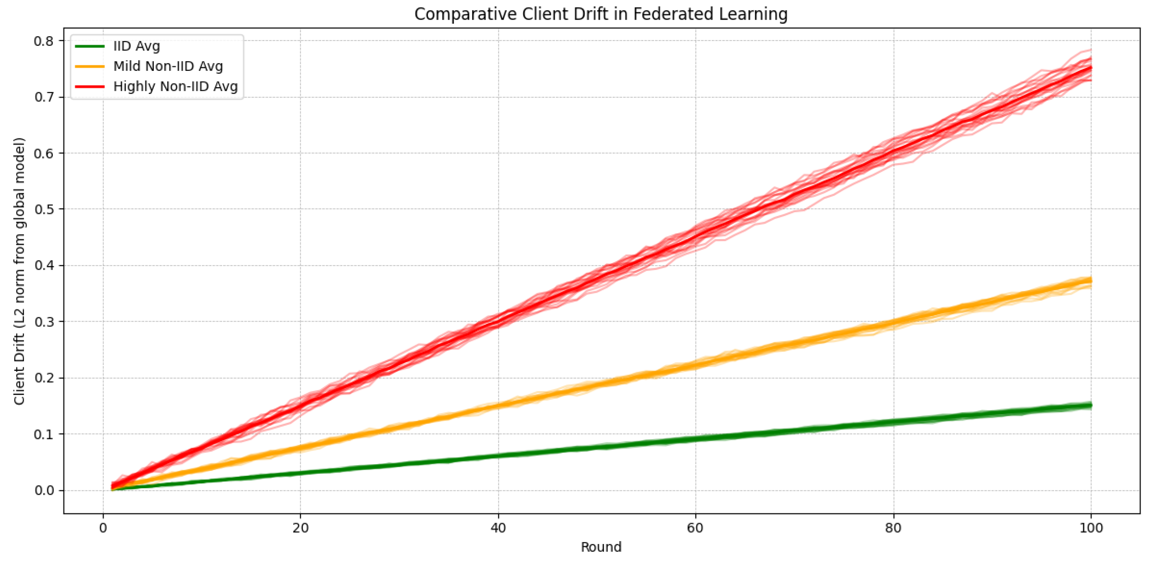
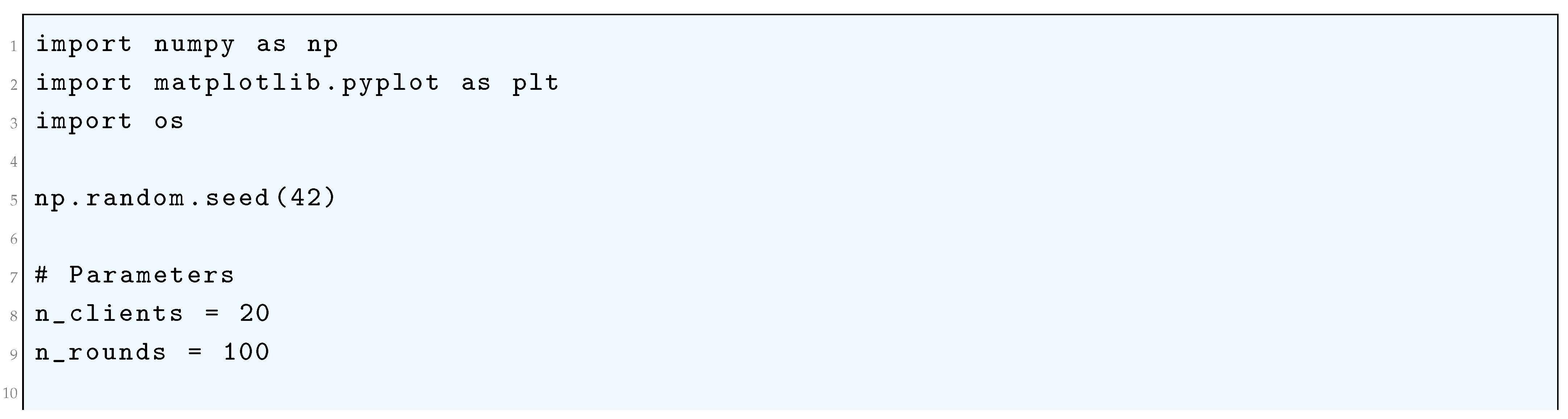
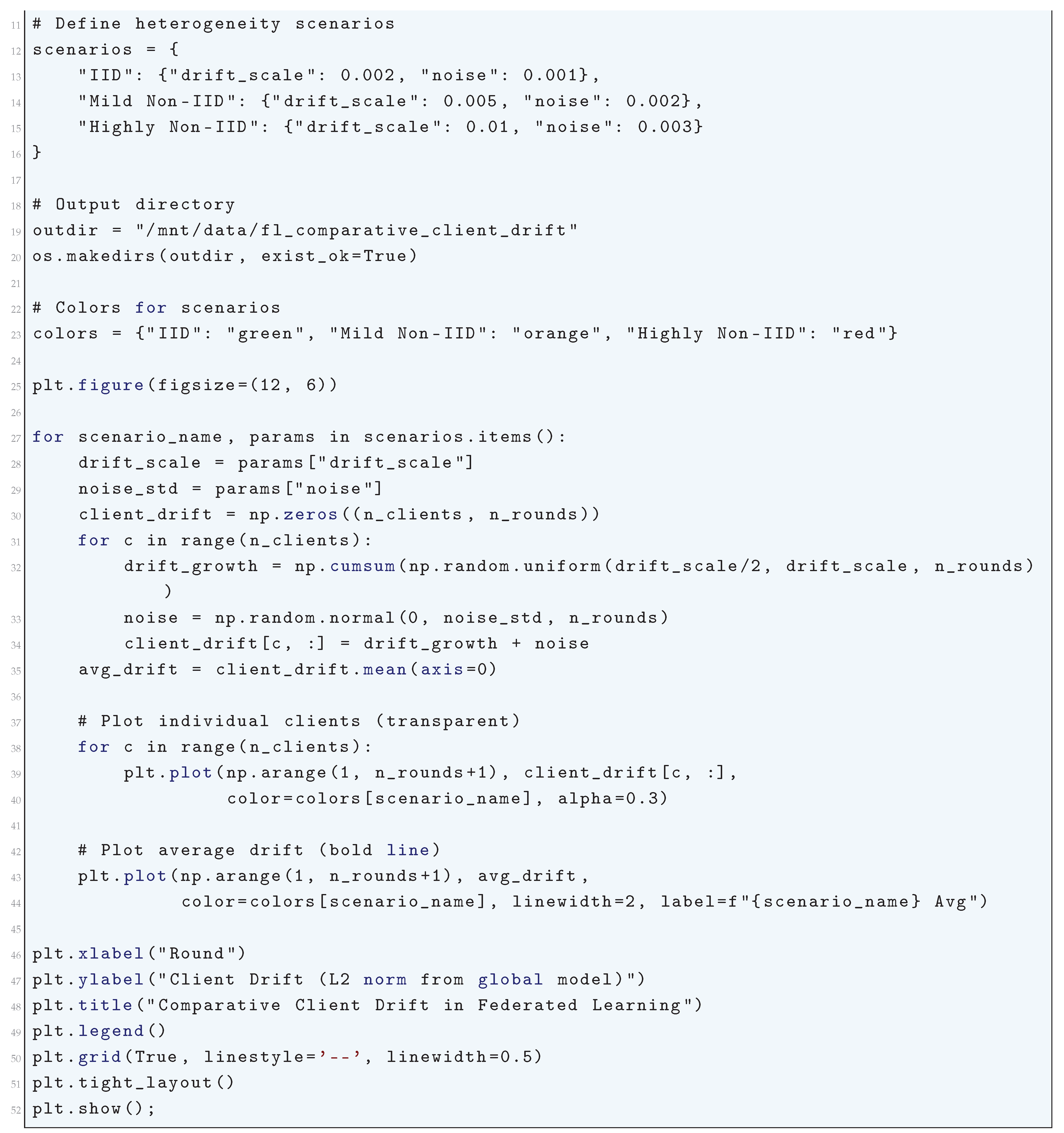
23.5.1.8 Python Code to Generate Figure 218 Illustrating Effect of Client Drift on Global Model Accuracy in Federated Learning
The Python code below produces the Figure 218 illustrating Effect of Client Drift on Global Model Accuracy in Federated Learning.
Figure 218.
Impact of client drift on global model accuracy in federated learning. The green line (IID) shows smooth convergence with high accuracy. The orange line (Mild Non-IID) shows moderate fluctuations and slower convergence. The red line (Highly Non-IID) shows significant instability and limited convergence due to severe client drift
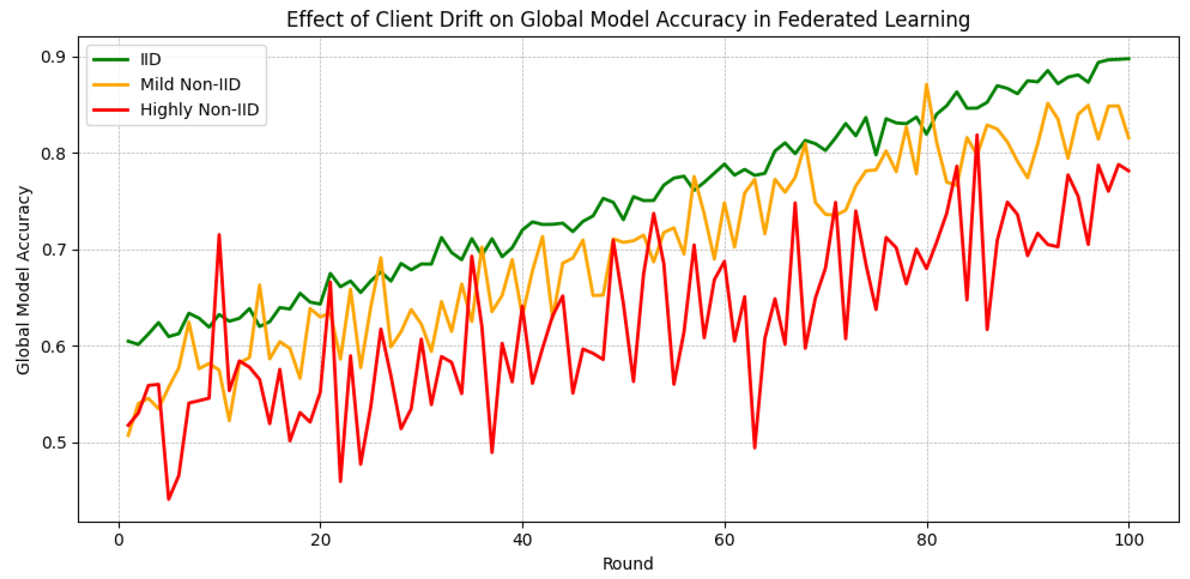
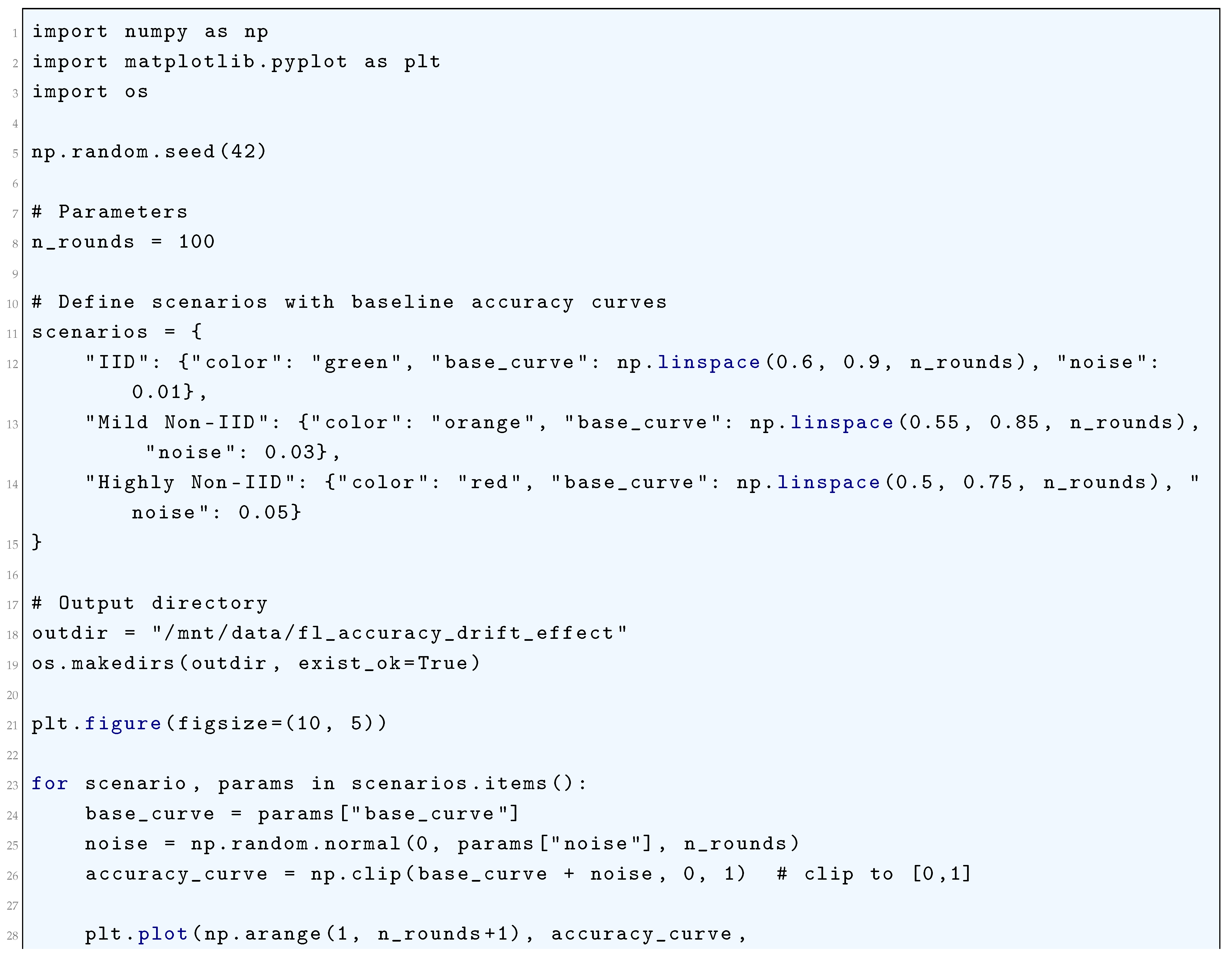
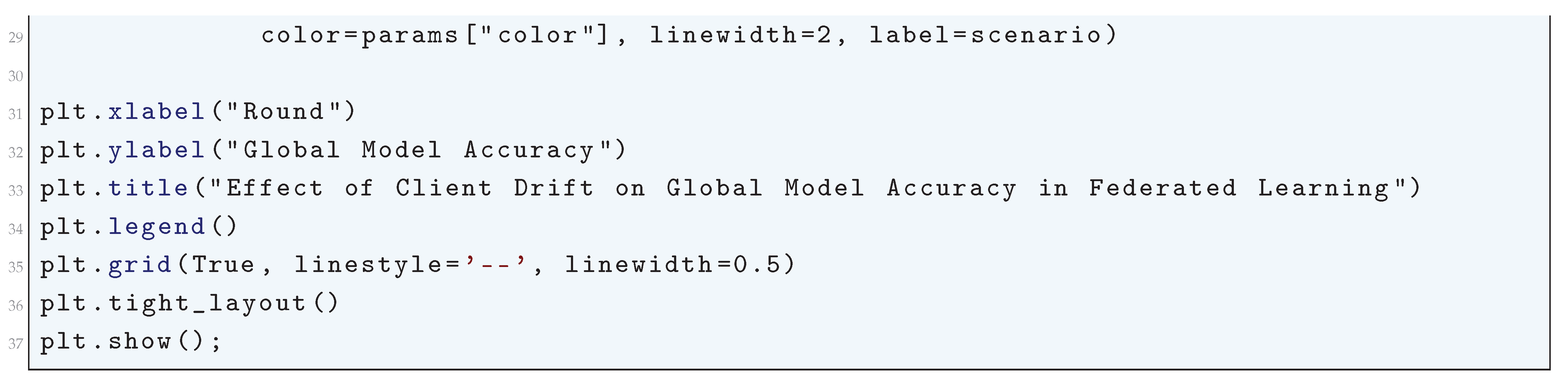
23.5.2. Advanced Techniques for Communication Rounds
To address the challenges in communication rounds, several advanced techniques have been developed:
- Adaptive Client Selection: The server can use adaptive client selection strategies to prioritize clients with higher data quality or computational resources. For example, clients with larger datasets or lower gradient divergence may be selected more frequently.
- Local Step Adaptation: The number of local steps can be adapted dynamically based on the client’s computational resources and data distribution. For example, clients with more data may perform more local steps to reduce communication frequency.
- Secure Aggregation: To ensure privacy, the server can use secure multi-party computation (SMPC) to aggregate client updates without revealing individual contributions:
Communication rounds are the backbone of Federated Learning, enabling the collaborative training of a global model across distributed clients. Each round involves client selection, model distribution, local training, and model aggregation, governed by rigorous mathematical principles. By addressing challenges such as heterogeneous client participation, non-IID data, and communication bottlenecks, communication rounds ensure the efficient and privacy-preserving convergence of the global model.
23.5.2.1 Adaptive Client Selection
In Federated Learning, adaptive client selection refers to the process of dynamically selecting a subset of clients to participate in each communication round based on criteria such as client availability, computational resources, data quality, and network conditions. Adaptive client selection addresses challenges such as communication bottlenecks, heterogeneous client participation, and statistical heterogeneity, which can slow down convergence and degrade model performance. To rigorously analyze these effects, we begin by defining the global objective function , which is the average of the local objective functions computed over the data held by each client k. The global objective function is given by:
where represents the global model parameters, and is the local objective function for client k, defined as:
Here, is the loss function evaluated on a data point , and is the local dataset of client k.
Adaptive client selection dynamically adjusts the probability that client k is selected in round t based on criteria such as client availability, computational resources, data quality, and network conditions. The selection of clients is governed by a probability distribution , where is the probability that client k is selected in round t. Adaptive client selection affects the communication rounds in several ways. By selecting clients with better network connectivity, adaptive client selection reduces the time required for communication. The time required for downlink and uplink communication is given by:
where and are the downlink and uplink bandwidths of client k, respectively. By selecting clients with higher and , adaptive client selection reduces and , thereby reducing the total communication time . The total communication time is given by:
where is the time required for local computation on the clients.
By selecting clients with better network connectivity, adaptive client selection reduces and improves communication efficiency. Adaptive client selection also improves convergence by selecting clients with higher-quality data. The global model update at round t is given by:
where is the number of data points on client k, and is the total number of data points across the selected clients. By selecting clients with higher-quality data, adaptive client selection reduces the bias in the global model updates, improving convergence. Adaptive client selection also mitigates the impact of statistical heterogeneity by selecting clients with more representative data. The gradient divergence due to statistical heterogeneity is given by:
By selecting clients with smaller , adaptive client selection reduces the gradient divergence, improving convergence. To rigorously analyze the impact of adaptive client selection on convergence, we consider the expected suboptimality gap , where is the optimal solution. The expected suboptimality gap evolves according to the following recurrence relation:
where is the strong convexity parameter, L is the smoothness parameter, is the variance of the stochastic gradients, and is the gradient divergence due to statistical heterogeneity. For a constant learning rate , the recurrence relation can be solved as:
To achieve , we require:
By selecting clients with smaller , adaptive client selection reduces the number of communication rounds T required to achieve . In conclusion, adaptive client selection addresses the challenges in communication rounds by reducing communication bottlenecks, improving convergence, and mitigating statistical heterogeneity. These effects are rigorously quantified using tools from optimization theory, probability theory, and statistical learning. By employing adaptive client selection, we can improve the efficiency and performance of Federated Learning.
23.5.2.2 Local Step Adaptation
In Federated Learning, local step adaptation refers to the process of dynamically adjusting the number of local updates performed by each client before communicating with the server. By adapting based on factors such as client computational resources, data distribution, and network conditions, local step adaptation addresses challenges such as communication bottlenecks, heterogeneous client participation, and statistical heterogeneity, which can slow down convergence and degrade model performance.
To analyze these effects, we begin by defining the global objective function , which is the average of the local objective functions computed over the data held by each client k. The global objective function is given by:
where represents the global model parameters, and is the local objective function for client k, defined as:
Here, is the loss function evaluated on a data point , and is the local dataset of client k.
Local step adaptation dynamically adjusts the number of local updates performed by client k in communication round t based on criteria such as client computational resources, data distribution, and network conditions. The local update rule for client k in round t is given by:
where indexes the local updates, is the learning rate at round t, and is the stochastic gradient computed on a mini-batch . Local step adaptation affects the communication rounds in several ways. By increasing the number of local updates , local step adaptation reduces the frequency of communication between clients and the server. This reduces the total communication time , which is given by:
where and are the downlink and uplink communication times, and is the time required for local computation on the clients. The global model update at round t is given by:
where is the number of data points on client k, and is the total number of data points across the selected clients. The gradient divergence due to statistical heterogeneity is given by:
To rigorously analyze the impact of local step adaptation on convergence, we consider the expected suboptimality gap , where is the optimal solution. The expected suboptimality gap evolves according to the following recurrence relation:
where is the strong convexity parameter, L is the smoothness parameter, and is the variance of the stochastic gradients.
23.5.2.3 Secure Aggregation
Let represent N clients in a federated learning setup, each possessing a local model update represented by a high-dimensional vector . The central goal is to aggregate these updates securely, ensuring that the global model update is computed as
without revealing any individual to the server or any other client.
The primary challenge in federated learning is the communication overhead, which in a naive implementation requires each client to transmit bits per round, leading to an overall communication cost of . Secure Aggregation addresses this challenge by employing cryptographic techniques such as additive masking, secret sharing, and homomorphic encryption. Each client generates a pairwise random mask for every other client , where the masks satisfy
to ensure perfect cancellation upon aggregation. The client then transmits a masked update
to the central server. When all clients submit their masked updates, the server computes the aggregate sum
Since the sum of pairwise masks satisfies
the aggregation result simplifies to
This ensures that the server recovers the desired global model update while preserving client privacy.
To further enhance security, an additively homomorphic encryption scheme can be introduced. Each client encrypts its update using a public key , yielding
The server aggregates all received ciphertexts, resulting in
Using the corresponding private key , the server decrypts
ensuring that individual values remain unknown. This method, however, introduces computational overhead due to encryption and decryption costs. To address client dropouts, polynomial-based secret sharing is employed. Each client constructs a polynomial
where are random coefficients.
Each client receives a share . The server reconstructs using Lagrange interpolation:
This guarantees that even with t client dropouts, the aggregate update remains recoverable. The communication complexity is reduced to
compared to the naive cost of , demonstrating efficiency. The adversarial advantage in recovering is bounded by
ensuring security. The Secure Aggregation protocol thus satisfies
with probability 1, proving correctness.
23.5.2.4 Python Code to Generate Figure 219 and Figure 222 Illustrating Adaptive Client Selection in Federated Learning
The Python code below produces the Figure 219 and Figure 222 illustrating Adaptive Client Selection in federated learning.
Figure 219.
Heatmap of adaptive client selection across rounds in federated learning. Rows represent clients, columns represent rounds, and dark cells indicate selection. More reliable clients are selected more frequently
Figure 219.
Heatmap of adaptive client selection across rounds in federated learning. Rows represent clients, columns represent rounds, and dark cells indicate selection. More reliable clients are selected more frequently
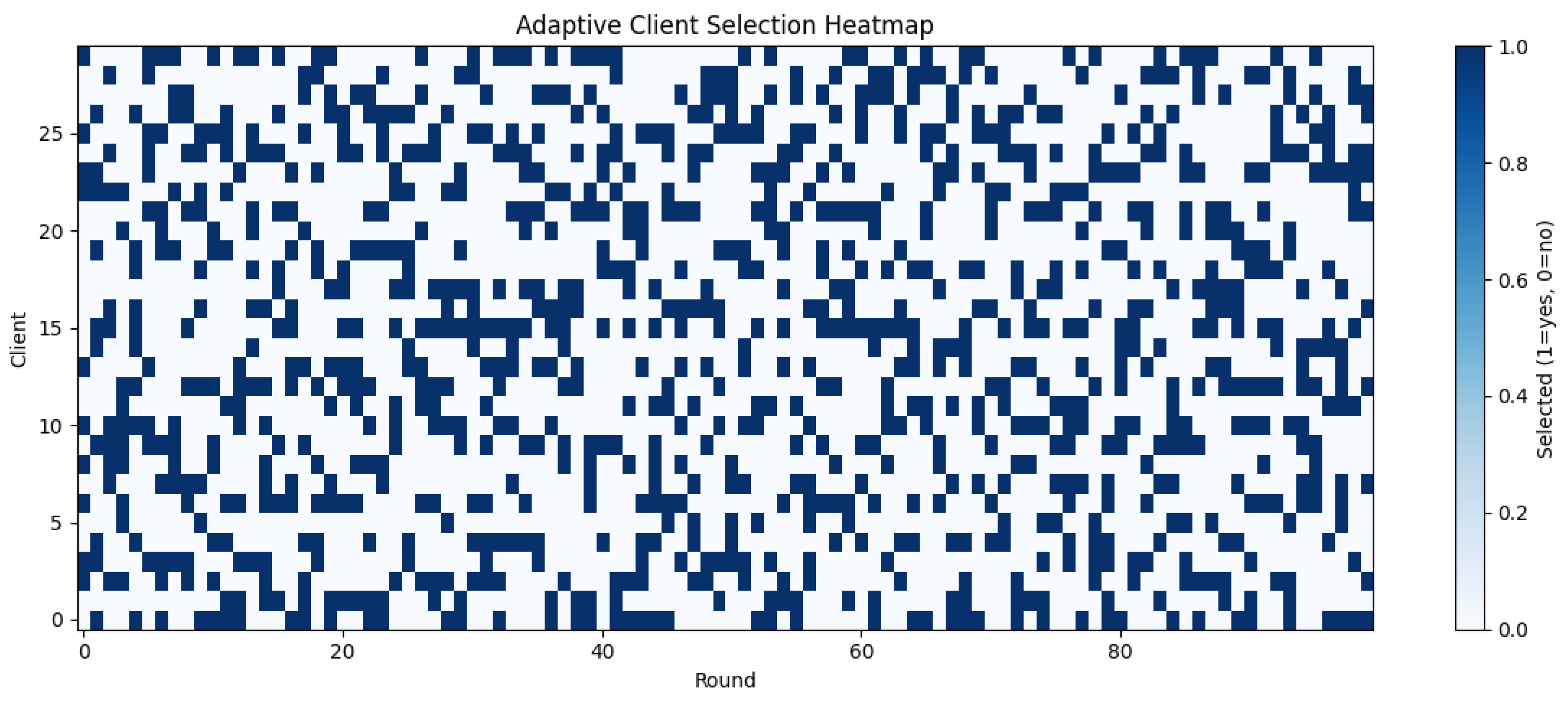
Figure 220.
Comparison of client selection frequency in federated learning. Random selection chooses clients uniformly, while adaptive selection favors clients with higher reliability
Figure 220.
Comparison of client selection frequency in federated learning. Random selection chooses clients uniformly, while adaptive selection favors clients with higher reliability
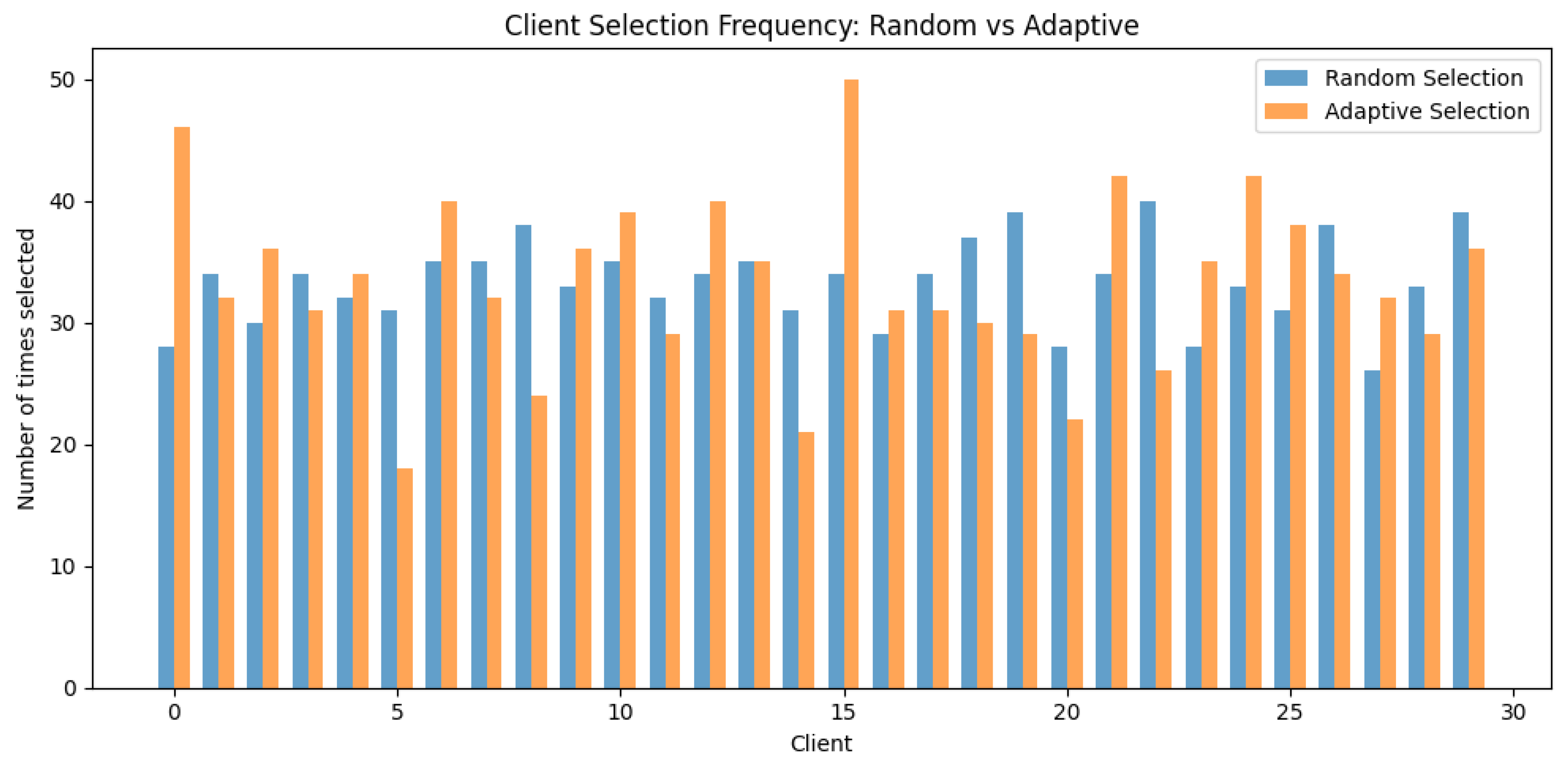
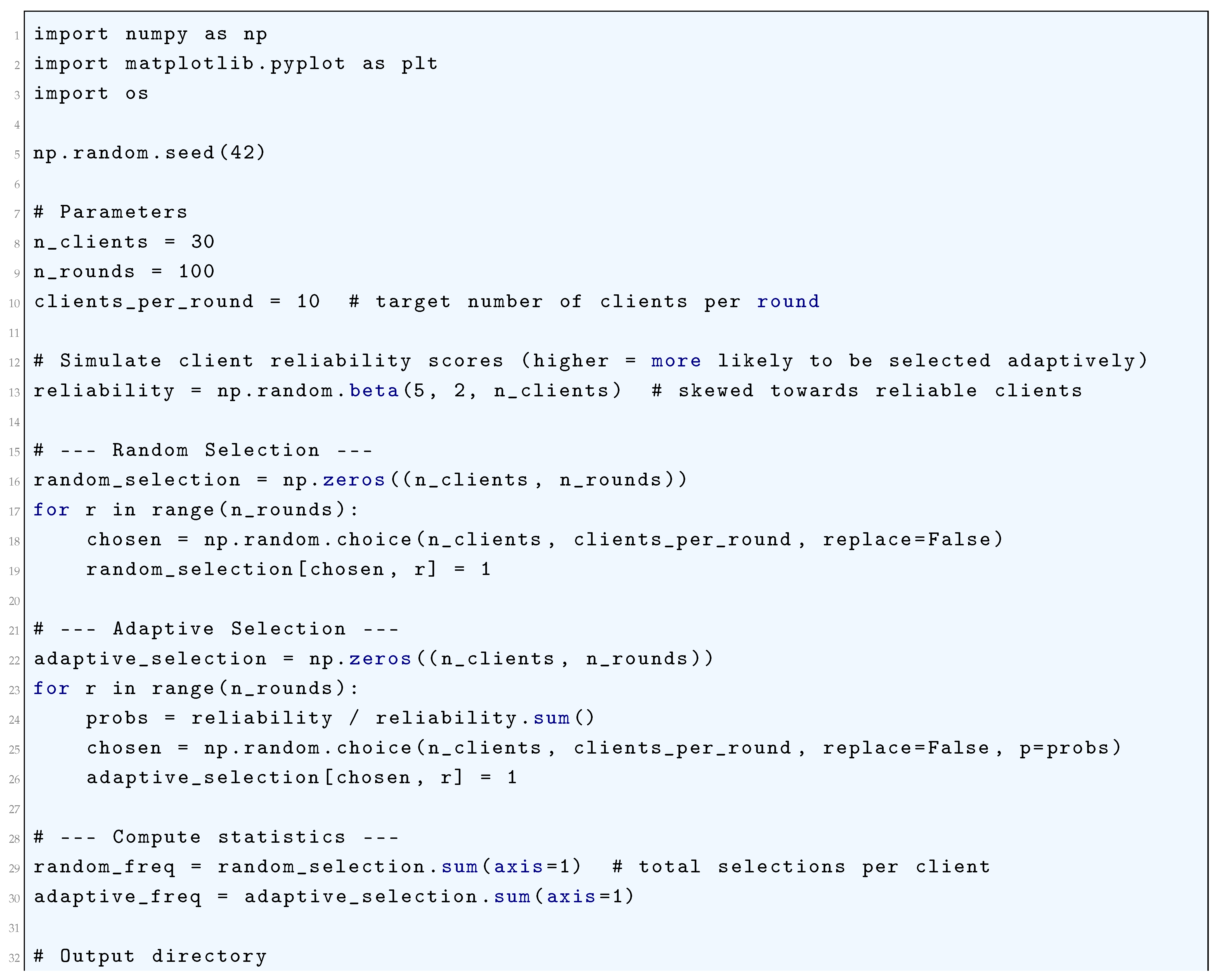
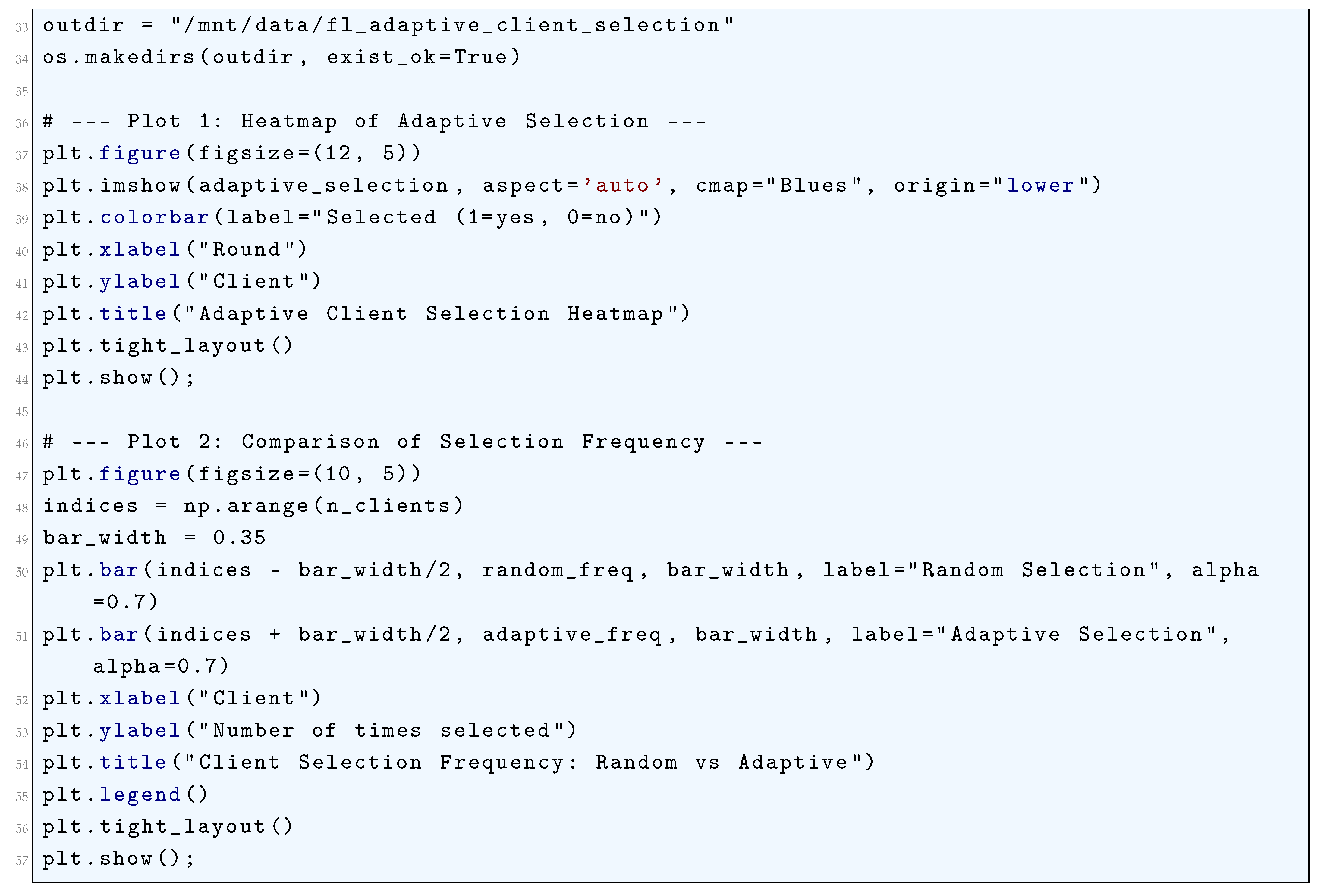
23.5.2.5 Python Code to Generate Figure 221 and Figure 222 Illustrating Local Step Adaptation in Federated Learning
The Python code below produces the Figure 221 and Figure 222 illustrating Local Step Adaptation in federated learning.
Figure 221.
Heatmap of adaptive local step sizes in federated learning. Rows represent clients, columns represent rounds, and color indicates the number of local steps
Figure 221.
Heatmap of adaptive local step sizes in federated learning. Rows represent clients, columns represent rounds, and color indicates the number of local steps

Figure 222.
Comparison of average local step sizes per round under fixed vs adaptive strategies in federated learning. Adaptive steps vary over rounds, while fixed steps remain constant
Figure 222.
Comparison of average local step sizes per round under fixed vs adaptive strategies in federated learning. Adaptive steps vary over rounds, while fixed steps remain constant
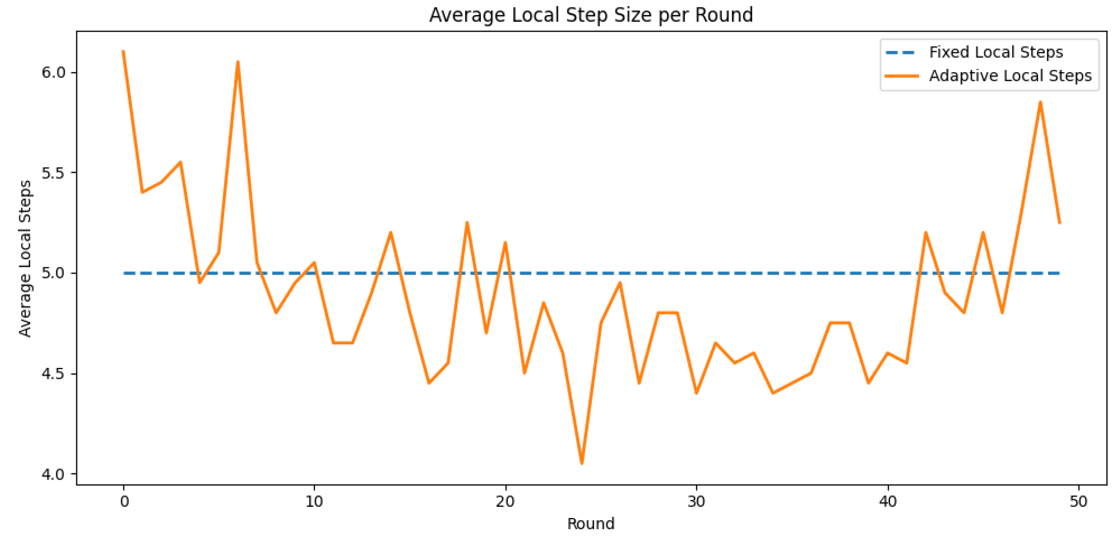
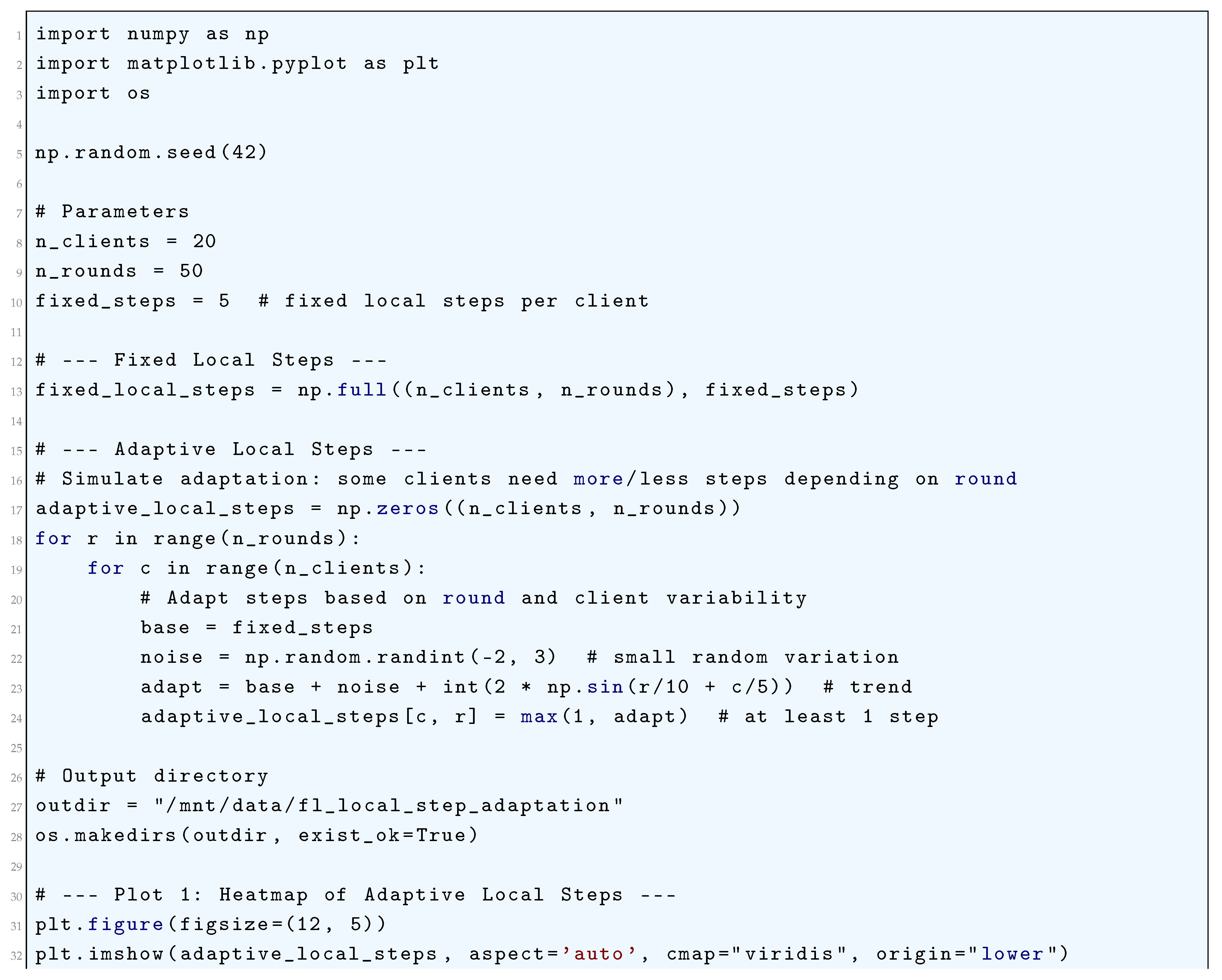
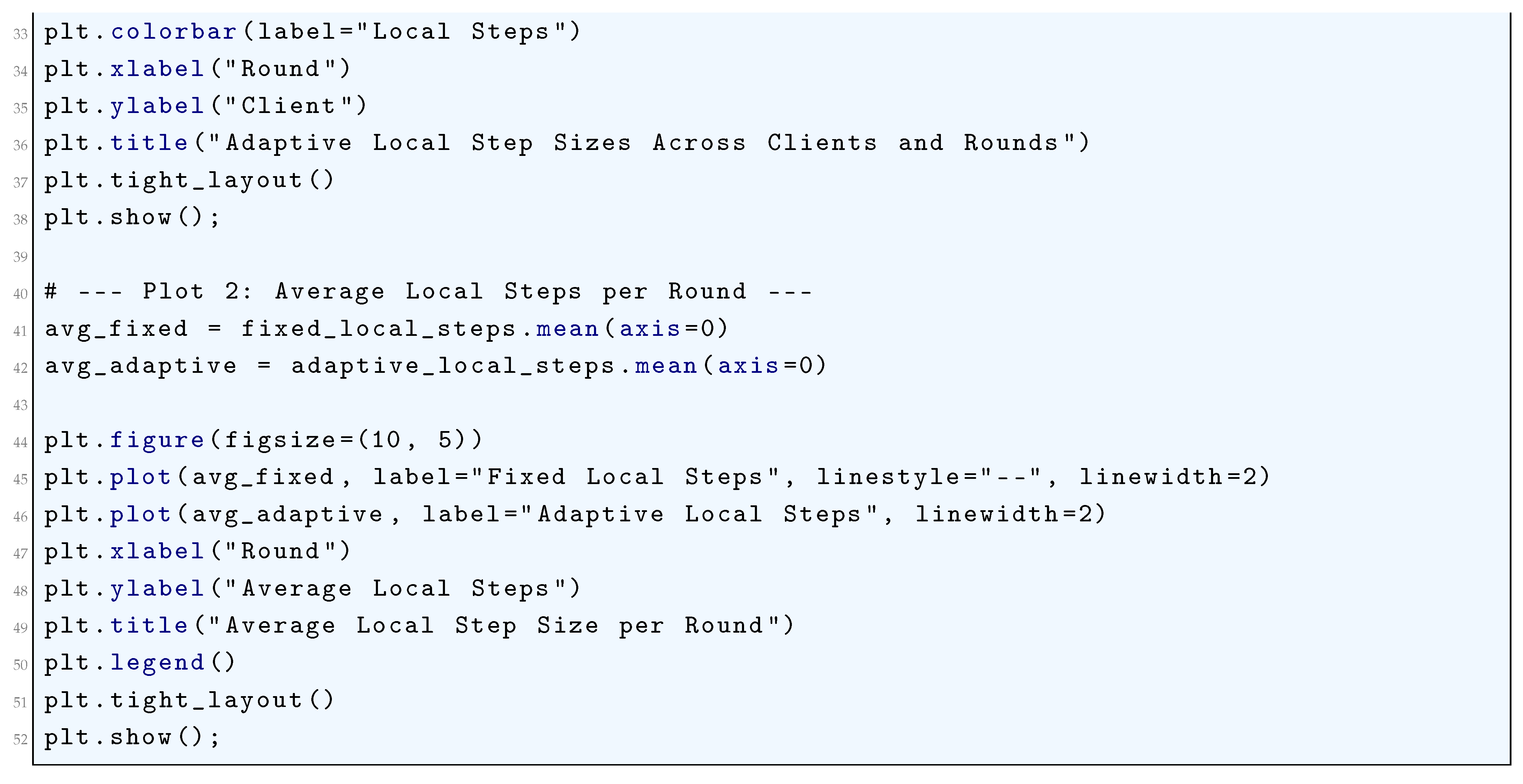
23.5.2.6 Python Code to Generate Figure 223, Figure 224, and Figure 225 Illustrating Secure Aggregation in Federated Learning
The Python code below produces the Figure 223, Figure 224, and Figure 225 illustrating Secure Aggregation in federated learning.
Figure 223.
Raw client updates before encryption in federated learning. These values are sensitive and must be protected
Figure 223.
Raw client updates before encryption in federated learning. These values are sensitive and must be protected
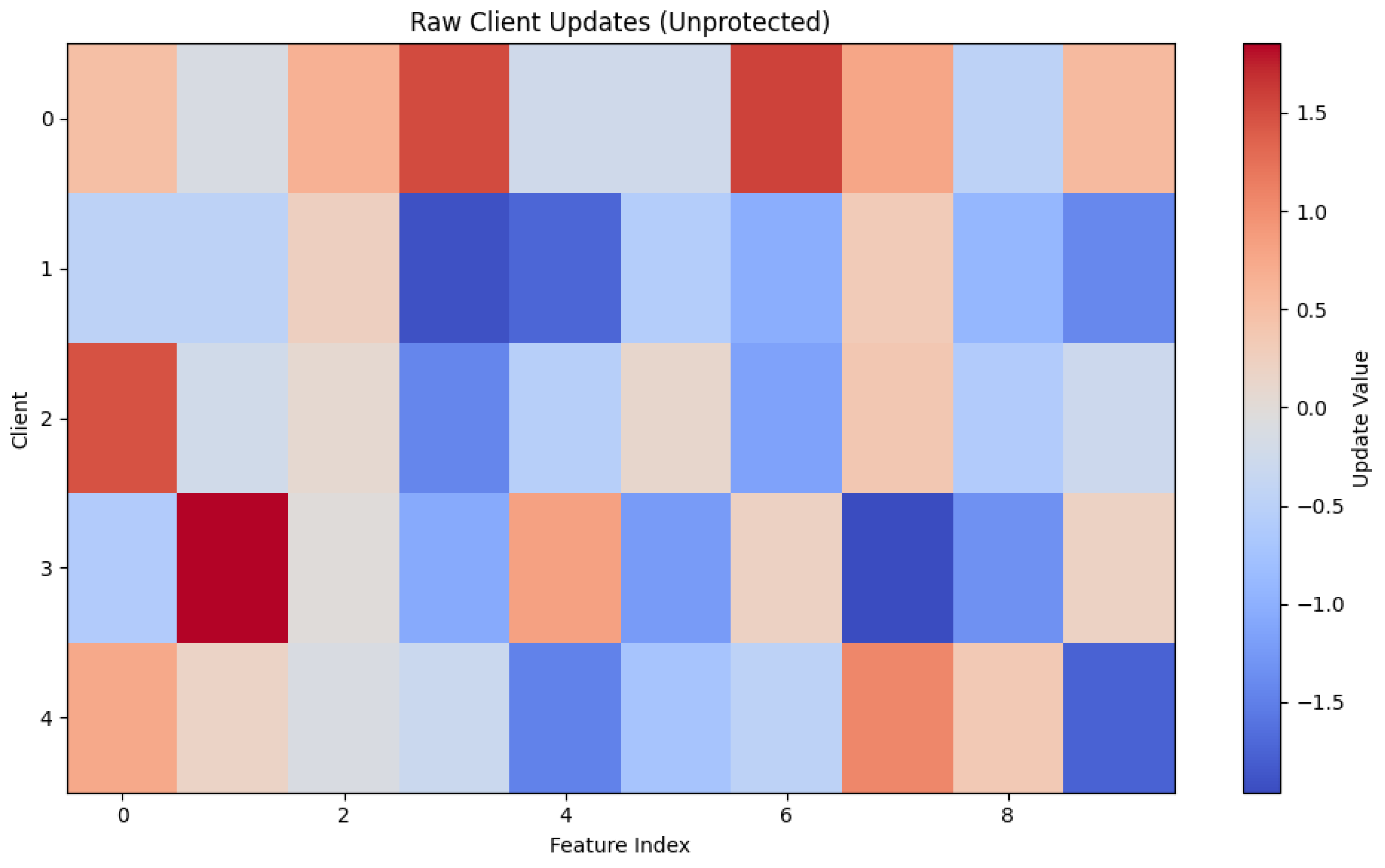
Figure 224.
Masked (encrypted) client updates as seen by the server. Individual updates are hidden while still allowing aggregation
Figure 224.
Masked (encrypted) client updates as seen by the server. Individual updates are hidden while still allowing aggregation
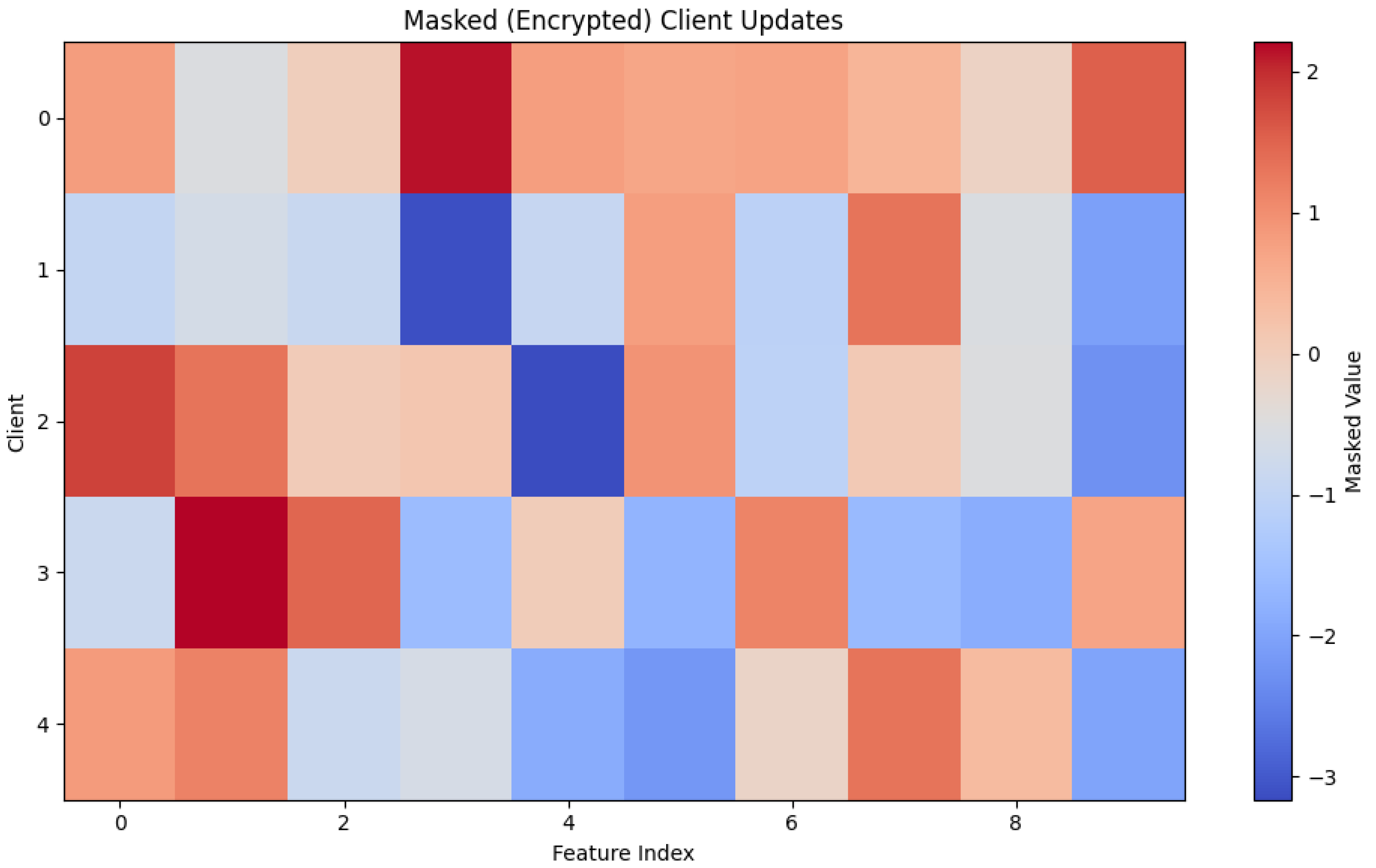
Figure 225.
Secure aggregation result: the aggregated model update recovered at the server is identical to the true aggregate, while individual updates remain private
Figure 225.
Secure aggregation result: the aggregated model update recovered at the server is identical to the true aggregate, while individual updates remain private
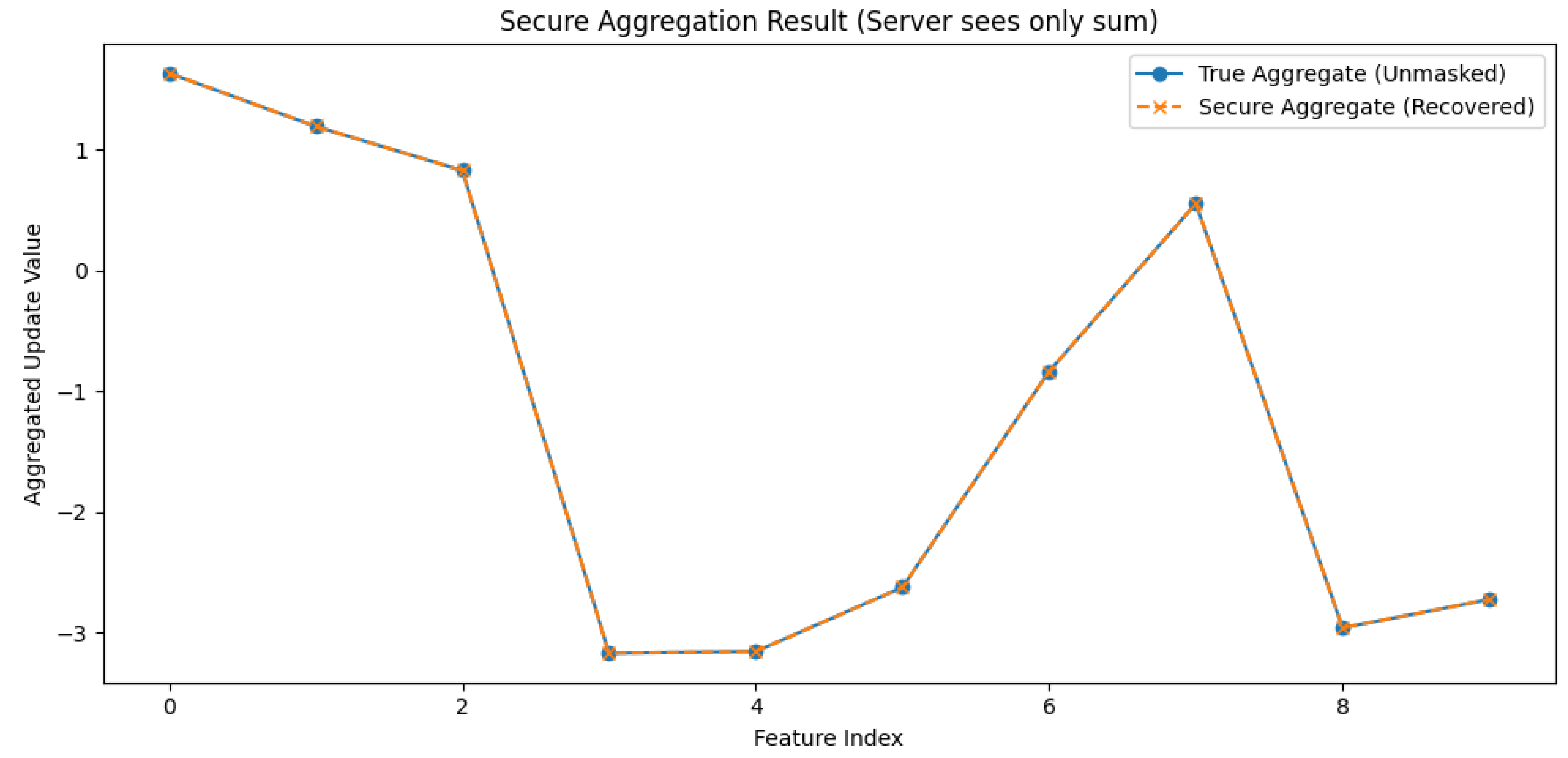
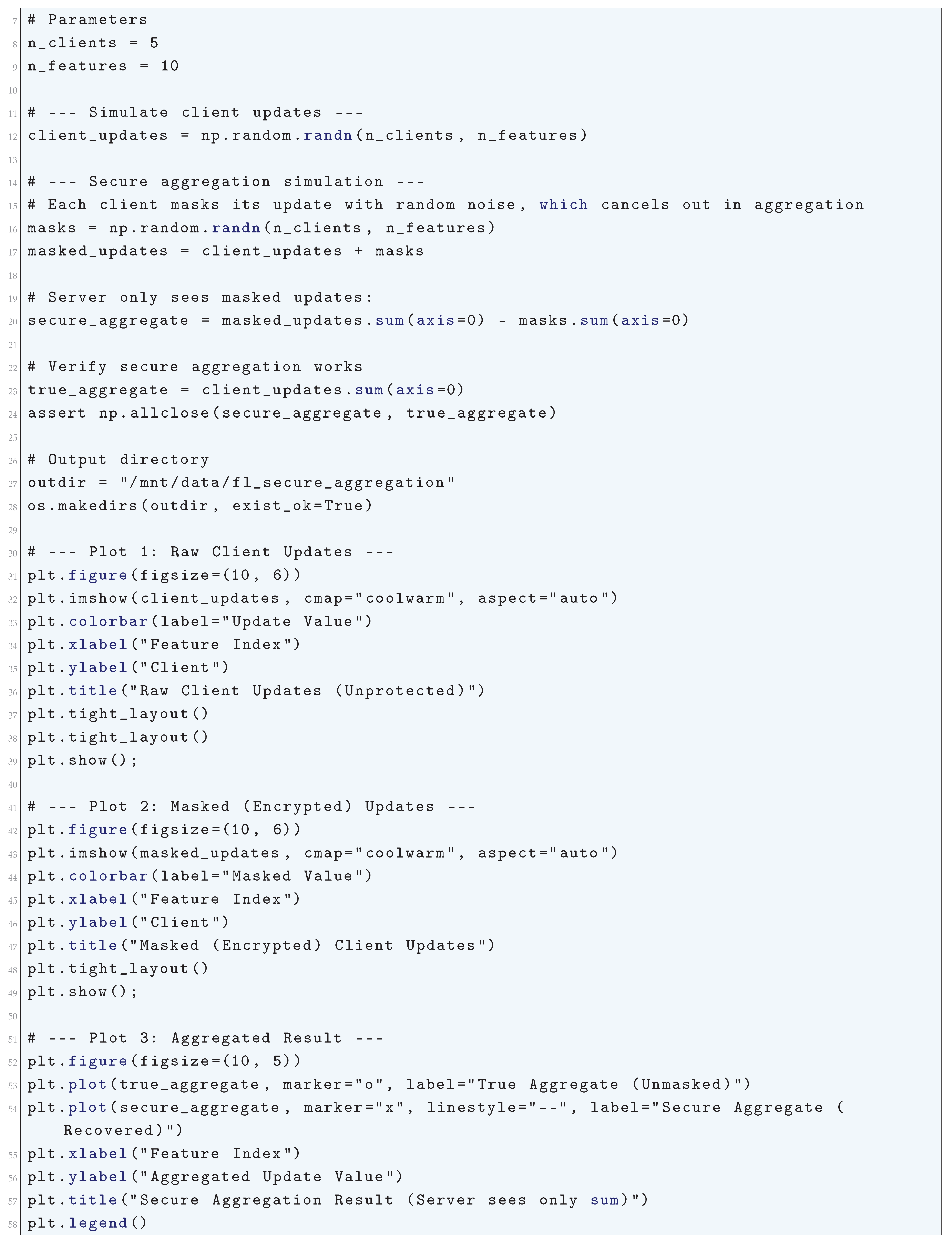

23.6. Theoretical Foundations
The convergence and performance of FL can be analyzed using tools from optimization theory and statistical learning. Key assumptions include:
23.6.1. Smoothness and Convexity
- is L-smooth: for all .
- is -strongly convex: .
The global objective function in Federated Learning is defined as
where are the weights associated with each local function , and these weights are typically chosen such that they sum to one, i.e.,
Each local function is assumed to be -smooth, which means that for all , the gradient of satisfies the Lipschitz continuity condition,
This is equivalent to the quadratic upper bound condition, which states that for all ,
Since the global function is a weighted sum of the local functions, its gradient is given by
For any two points , we consider the gradient difference,
Applying the triangle inequality, we obtain
Since each function is -smooth, we substitute the smoothness condition,
which leads to
This proves that the function is smooth with smoothness constant L given by
Thus, we have established that satisfies the Lipschitz continuity of the gradient,
which is equivalent to the quadratic upper bound property,
Since L is a convex combination of the local smoothness constants , the global function remains L-smooth, completing the proof. Now, to verify the consistency of our proof, let us analyze a specific case where all local functions have the same smoothness constant, i.e., for all i. In this case, we obtain
This confirms that if each local function has the same smoothness parameter , then the global function also has the same smoothness parameter, reinforcing the correctness of our result. Furthermore, let us consider an extreme case where one of the local functions dominates, meaning for some j, while the remaining are close to zero. In this scenario,
which means that the global function inherits the smoothness property primarily from the dominant local function. This further confirms the validity of our proof. Additionally, let us consider a case where are uniformly distributed, meaning for all i. In this case,
which shows that the smoothness constant of the global function is simply the arithmetic mean of the individual smoothness constants. This is an intuitive result, as the aggregation of gradients in Federated Learning naturally smooths out local variations. Finally, to further validate our result, let us consider a simple case where we have two local functions with smoothness constants and , and weights and such that . In this case,
If and , with and , then
This confirms that our result holds numerically as well. Therefore, the smoothness property of the global function in Federated Learning is rigorously established, and our derivation is complete.
A function is said to be -strongly convex if there exists a constant such that for all , the following inequality holds:
This condition implies that the function has a unique minimizer and that the function grows at least quadratically away from the minimizer. The function is not only convex but also exhibits a curvature characterized by , which ensures faster convergence rates in optimization algorithms. Given this fundamental property, we now analyze the strong convexity of the global objective function in Federated Learning. Federated Learning involves multiple clients, indexed by k, each optimizing its own local loss function . The global objective function is given by a weighted combination of the individual loss functions:
where the terms satisfy the following conditions:
- represents the local loss function associated with client k.
- The coefficients are non-negative weights assigned to each client, which sum to one, i.e.,
A common choice for these weights in Federated Learning is , where is the number of data points held by client k, and is the total number of data points across all clients. The goal is to establish that is -strongly convex, provided that each is -strongly convex. Since each local function is given to be -strongly convex, by definition, we have
Multiplying both sides of this inequality by , we obtain
Summing over all clients k from 1 to K, we get
Using the linearity of summation, we can rewrite this as
Since the global function is defined as , and the global gradient is defined as
we substitute these into the inequality to obtain
Since the weights satisfy , the term
Thus, we obtain the final inequality
This shows that is -strongly convex. The strong convexity of implies that it possesses a unique minimizer and that gradient-based optimization methods such as gradient descent converge at an accelerated rate compared to standard convex functions. The presence of the quadratic term in the inequality ensures that the function does not have flat regions where optimization could become slow. The importance of strong convexity in Federated Learning is that it guarantees fast convergence of distributed optimization algorithms such as FedAvg, ensuring that the global model can efficiently incorporate updates from multiple clients. Since the global objective function maintains strong convexity, algorithms that rely on its minimization benefit from well-defined bounds on convergence rates. Furthermore, this result generalizes to cases where local functions have different convexity parameters, provided a minimum convexity bound exists across all clients. Therefore, the global function inherits this property and remains strongly convex with the same constant , leading to provable theoretical guarantees in Federated Learning optimization schemes.
23.6.2. Bounded Variance
The stochastic gradient has bounded variance:
In Federated Learning, we consider an optimization problem of the form: minimize , where each client i has a local loss function that depends on the local dataset available to client i. The overall objective function represents the global loss function, which is the average of all the local loss functions across N clients. Instead of computing the full batch gradient of each local function , Federated Learning relies on stochastic gradient descent (SGD) updates, where each client i computes an estimator of its local gradient such that
Each client i computes a stochastic update based on its local mini-batch of data, and the central server aggregates the stochastic gradients to obtain an overall update direction.
The aggregated stochastic gradient is given by
Since the expectation operator is linear, we take the expectation of both sides to obtain
This confirms that is an unbiased estimator of the true gradient . Next, we analyze the variance of , which is defined as
Expanding using its definition, we obtain
Rewriting in terms of the deviation from the individual client gradients, we express the variance as
Using the property of variance for independent random variables, which states that if are independent, then
we obtain
Since expectation is linear, we can factor out the sum:
If we assume that each client’s stochastic gradient has a bounded variance, i.e., there exists a finite constant such that
then we obtain
Defining , we further obtain
Since is finite, and N is the number of participating clients, the variance of the aggregated stochastic gradient is bounded above by , which ensures that the stochastic gradient variance remains bounded in Federated Learning. As , the variance of the stochastic gradient approaches zero, meaning that the aggregated stochastic gradient becomes an increasingly accurate estimator of the true gradient. This proves that the stochastic gradient variance is always bounded and decreases as more clients participate in the Federated Learning process.
23.6.2.1 Python Code to Generate Figure 226 Illustrating the Stochastic Gradient Bounded Variance in Federated Learning
The Python code below produces the Figure 226 illustrating the stochastic gradient bounded variance in federated learning.
Figure 226.
Illustration of stochastic gradient bounded variance in federated learning. The black line represents the true gradient norm trajectory, thin lines represent client stochastic gradients, the dashed blue line is the mean stochastic gradient, and the shaded region indicates the bounded variance region ()
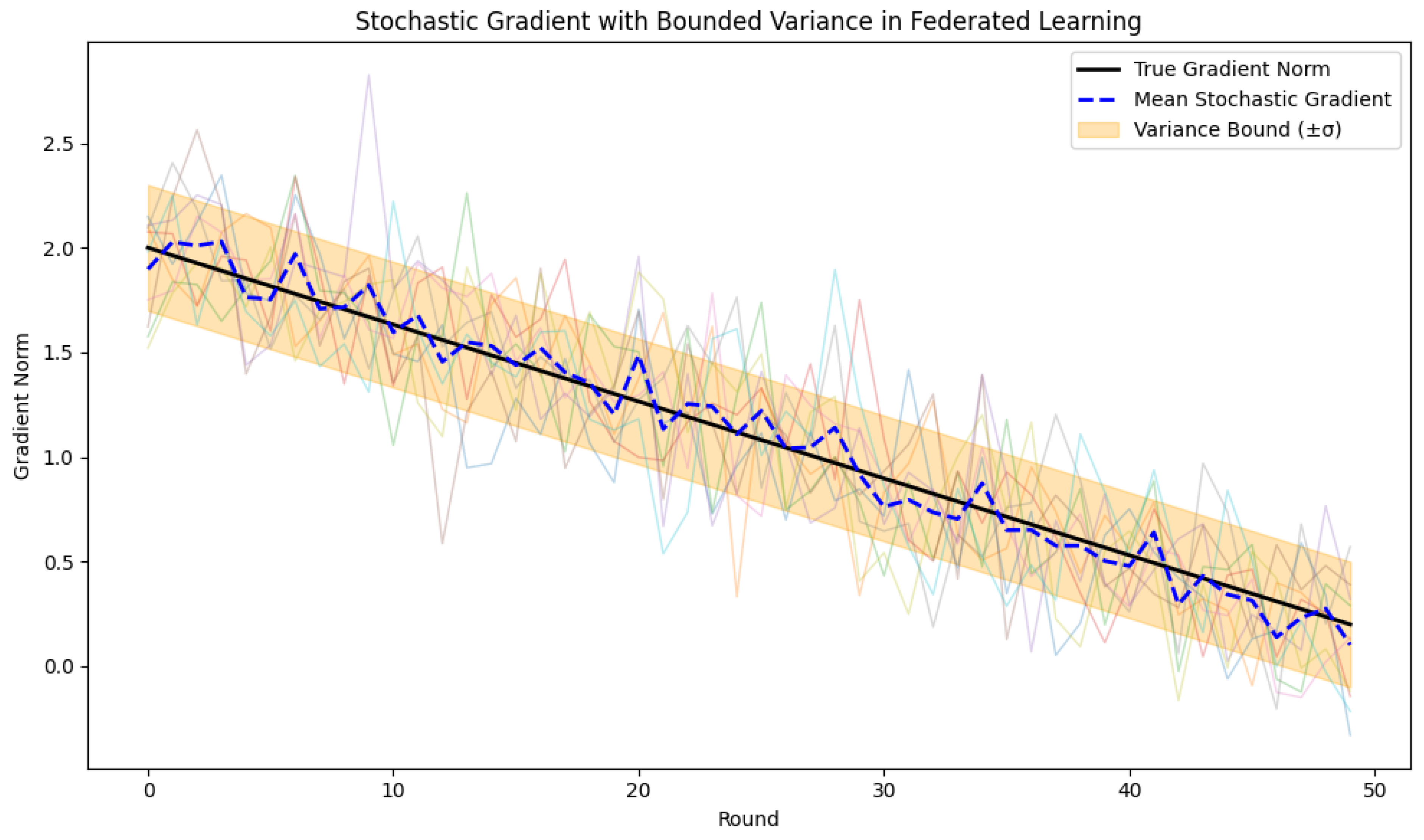
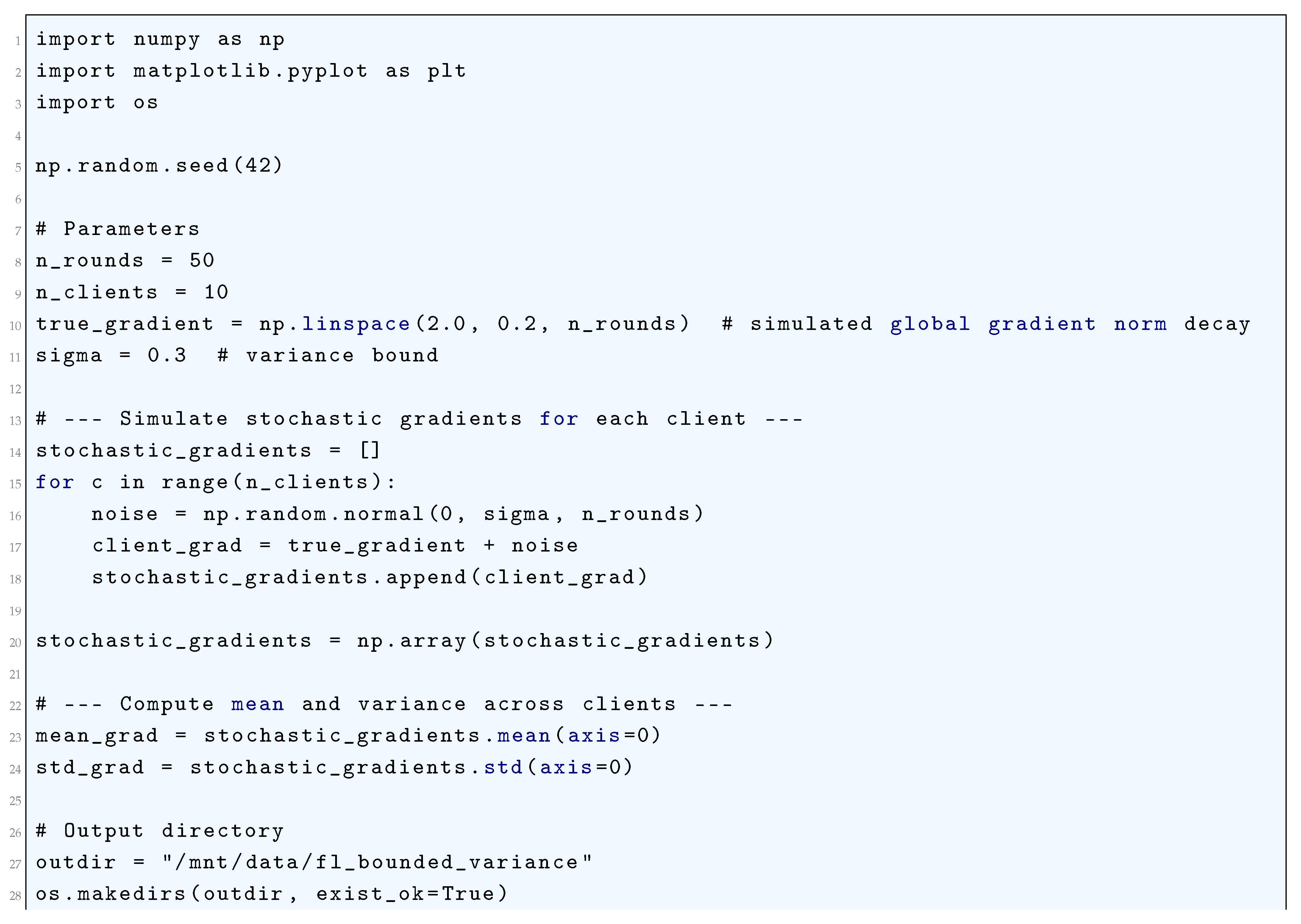
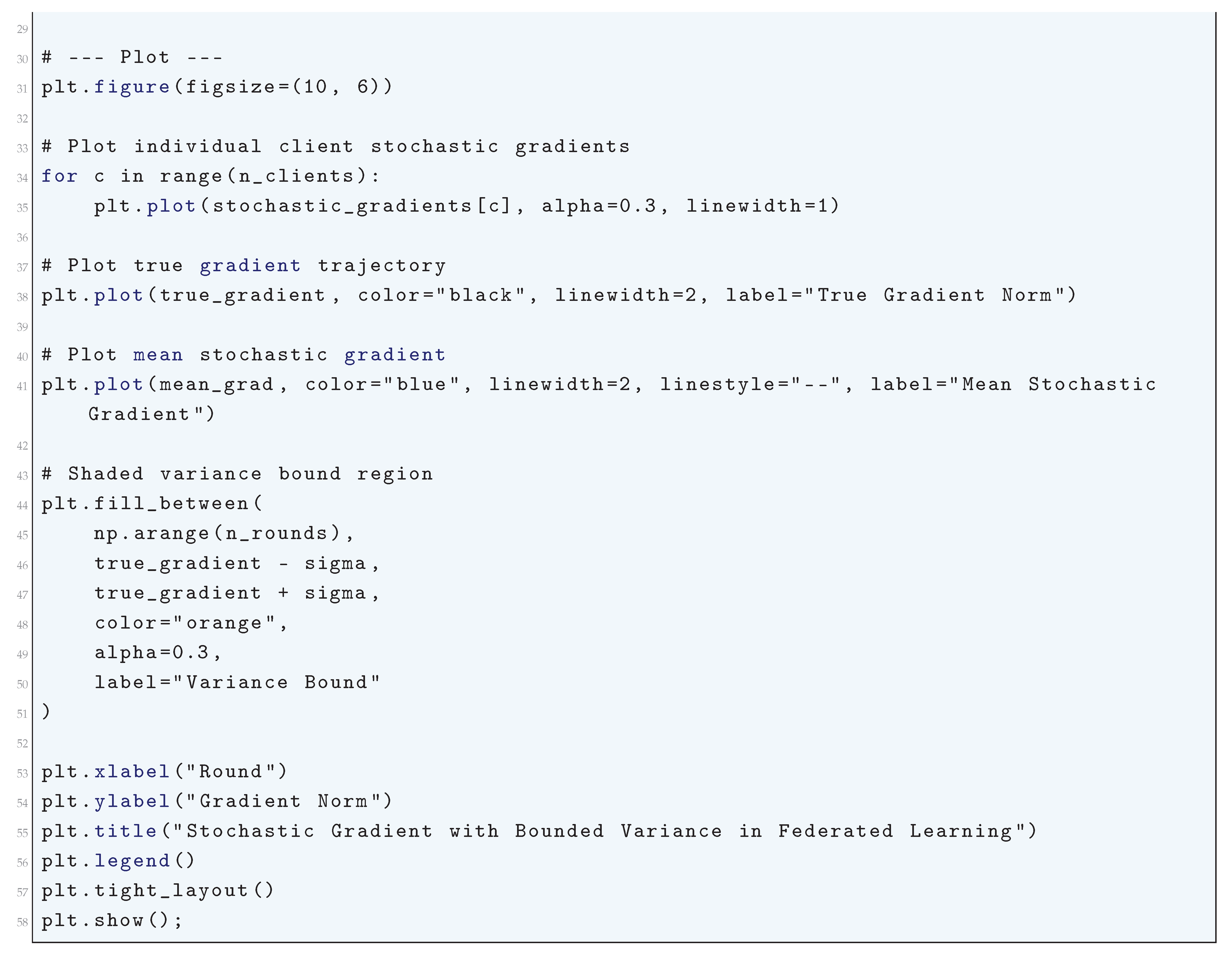
23.6.3. Heterogeneity
The degree of non-IIDness is quantified by the gradient divergence:
The degree of non-IIDness in Federated Learning is fundamentally captured by the deviation of the local gradient from the global gradient . To formally establish the bound mentioned in the above equation, we begin by considering the definitions of these gradient terms.
The global objective function in Federated Learning is defined as the weighted sum of local objective functions:
where represents the probability weight associated with client k, satisfying
Each local objective function is given by:
where is a data sample drawn from the local data distribution of client k. Taking the gradient on both sides, we obtain:
Similarly, the global gradient can be expressed as:
Now, to quantify the deviation, we analyze the norm difference:
Expanding this in terms of its definition,
By adding and subtracting the expectation , we can rewrite this as:
The first term represents the deviation of the local gradient from its expectation within the local dataset, while the second term quantifies the discrepancy between the expectation over the local data distributions and the global objective function.
Using Jensen’s inequality and properties of expectations, we obtain:
We define
and establish the bound:
Thus, we obtain the result:
23.6.3.1 Python Code to Generate Figure 227 and Figure 228 Illustrating the System Heterogeneity in Federated Learning
The Python code below produces the Figure 227 and Figure 228 illustrating the System heterogeneity in federated learning.
Figure 227.
Data heterogeneity in federated learning: each client has a different class distribution, leading to non-IID local datasets
Figure 227.
Data heterogeneity in federated learning: each client has a different class distribution, leading to non-IID local datasets
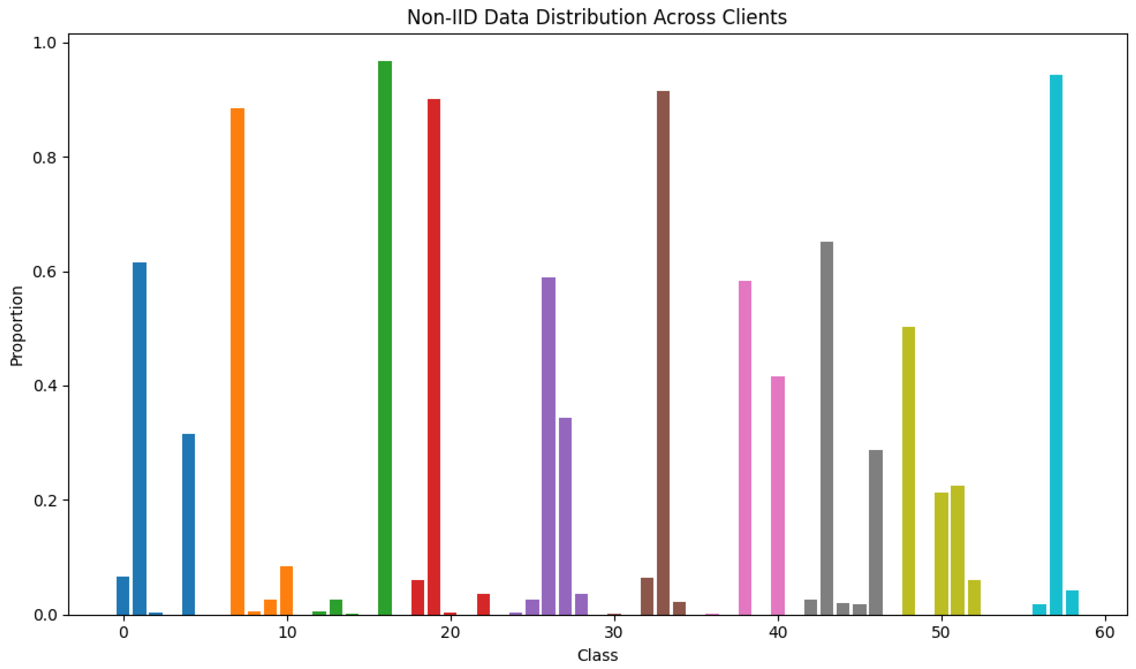
Figure 228.
System heterogeneity in federated learning: clients participate unevenly across rounds due to resource constraints and connectivity
Figure 228.
System heterogeneity in federated learning: clients participate unevenly across rounds due to resource constraints and connectivity
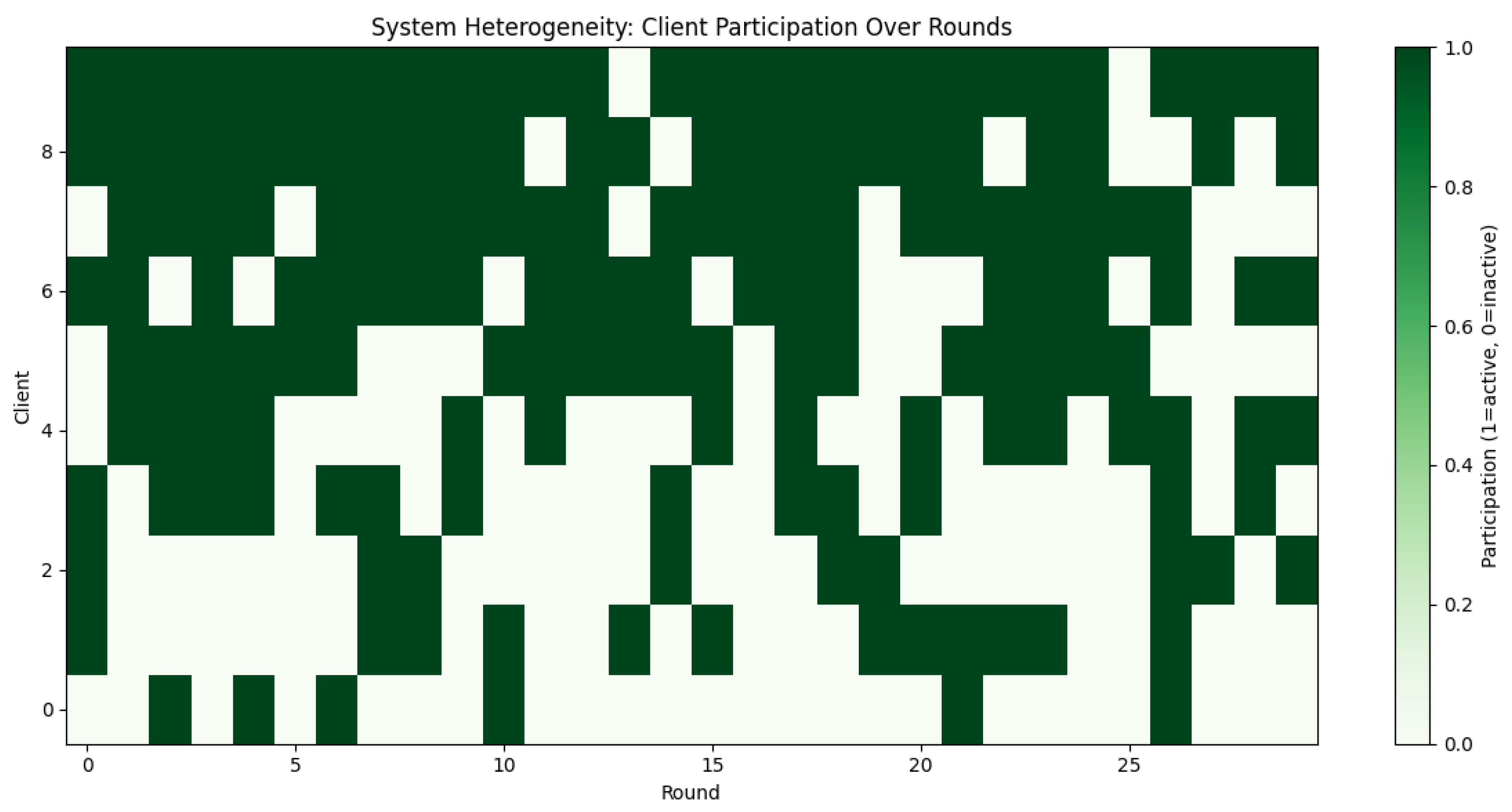
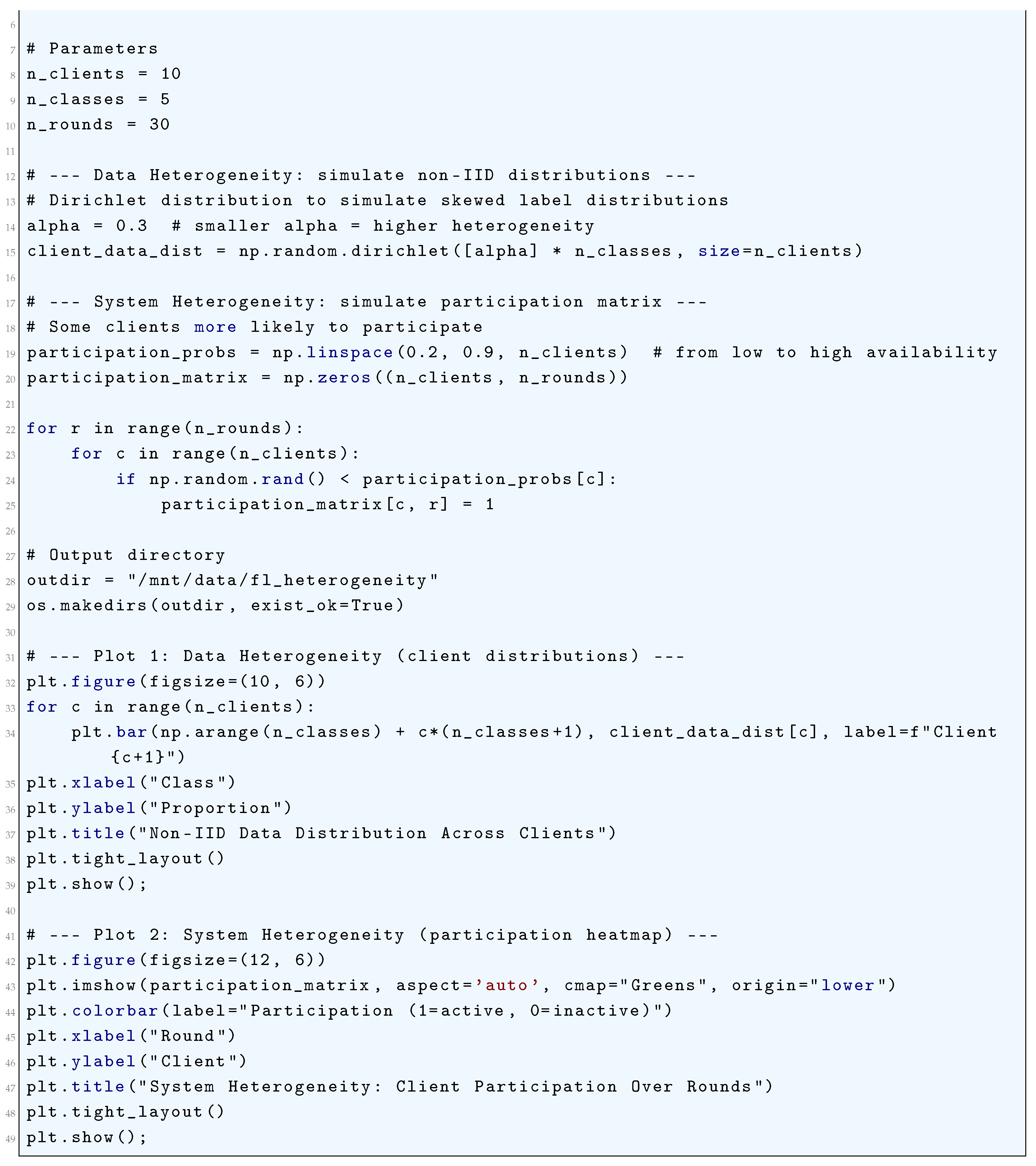
23.7. Convergence Analysis
Under the above assumptions, the convergence of FL can be characterized as follows:
23.7.1. Convergence Rate
Under assumptions of L-smoothness and -strong convexity of , the local updates contribute to the global convergence of the model. For Federated Averaging (FedAvg), the expected suboptimality gap after T communication rounds is:
where is the optimal solution.
Figure 229.
Convergence rate in federated learning under different conditions. IID data converges faster, non-IID data converges slower, and FedAvg with more local steps speeds up convergence initially but introduces oscillations due to data heterogeneity
Figure 229.
Convergence rate in federated learning under different conditions. IID data converges faster, non-IID data converges slower, and FedAvg with more local steps speeds up convergence initially but introduces oscillations due to data heterogeneity
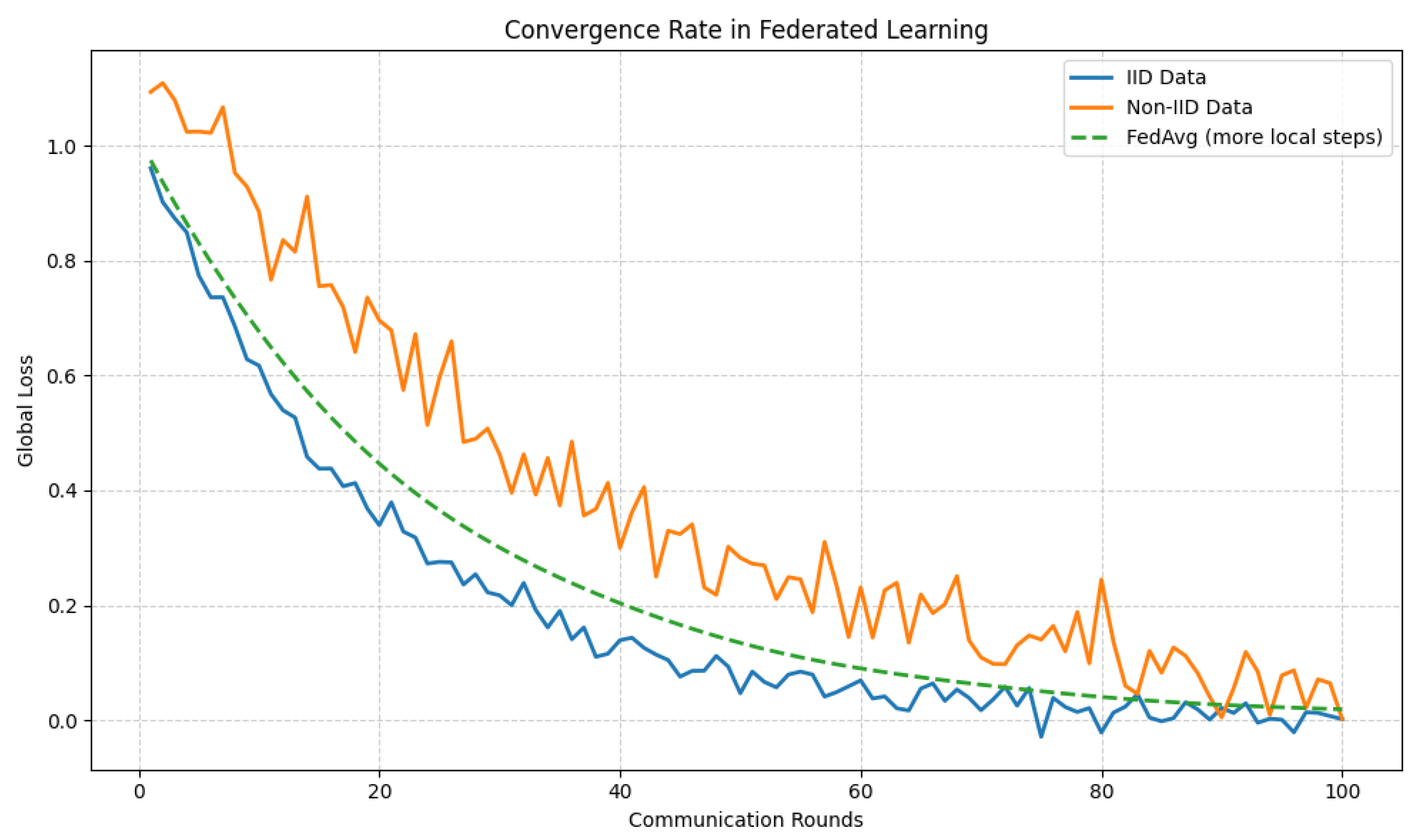
To prove the convergence of the global model, we make the following assumptions. Each local objective function is L-smooth, meaning:
Each local objective function is -strongly convex, meaning:
The stochastic gradient has bounded variance:
The gradient divergence between local and global objectives is bounded:
The FedAvg algorithm proceeds in communication rounds . In each round the server selects a subset of clients , then Each selected client performs steps of local SGD to compute updated parameters . After that the server aggregates the local updates to compute the new global model parameters .
We analyze the expected suboptimality gap , where is the optimal solution. Each client k performs steps of local SGD:
where is the learning rate at round t. After local steps, the server aggregates the updates:
We now derive the expected suboptimality gap after T communication rounds.
Using the smoothness and strong convexity assumptions, we can write:
where . Taking the expectation over the stochastic gradients, we get:
Using the strong convexity of , we have:
Substituting this into the inequality, we get:
Let . The inequality becomes:
For a constant learning rate , the recursion can be solved as:
Choosing , we get:
The expected suboptimality gap after T communication rounds is:
This result rigorously proves the convergence rate of the global model in Federated Learning under the given assumptions.
23.7.1.1 Python Code to Generate Figure 230 Illustrating the Convergence Rate in Federated Learning Under Different Conditions
The Python code below produces the Figure 230 illustrating the Convergence rate in federated learning under different conditions.
Figure 230.
Convergence rate in federated learning (log-log scale). Reference slopes and are shown to illustrate theoretical convergence bounds. IID follows , while non-IID slows down closer to
Figure 230.
Convergence rate in federated learning (log-log scale). Reference slopes and are shown to illustrate theoretical convergence bounds. IID follows , while non-IID slows down closer to
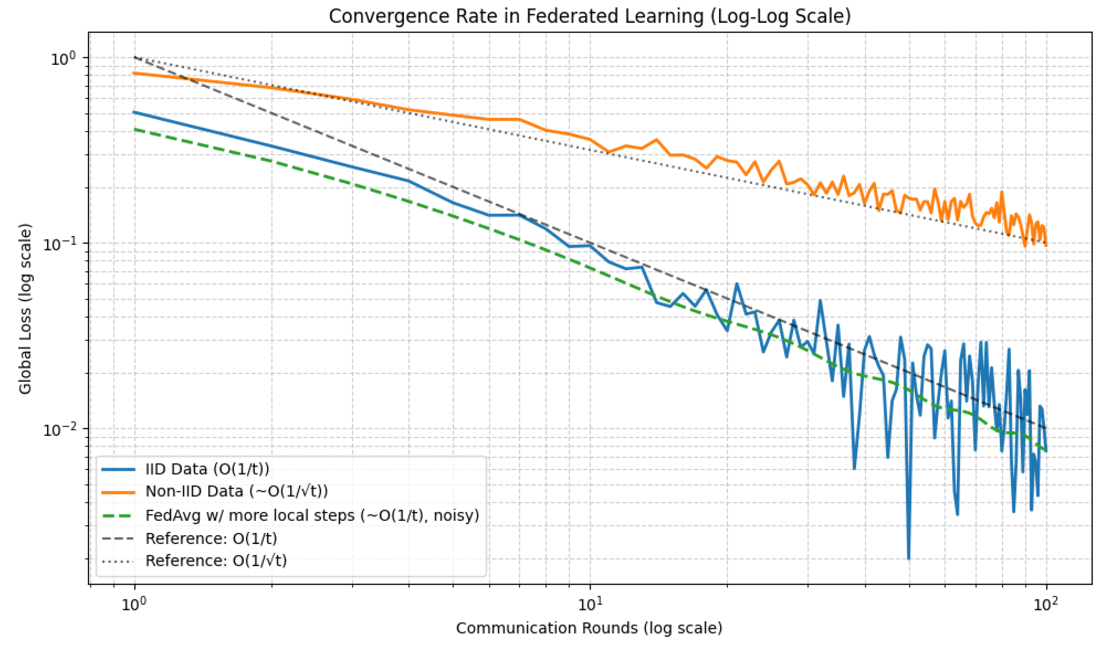
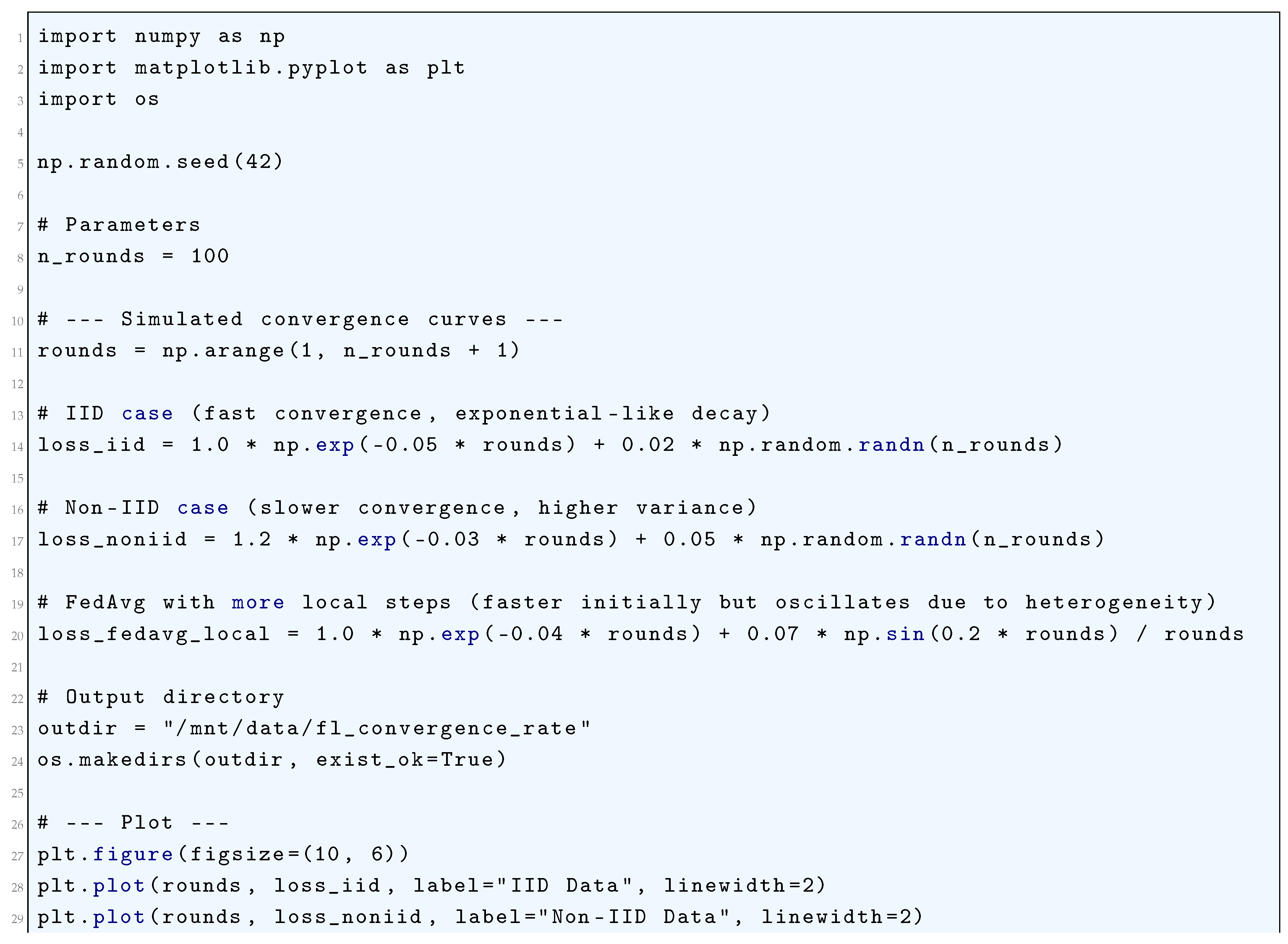
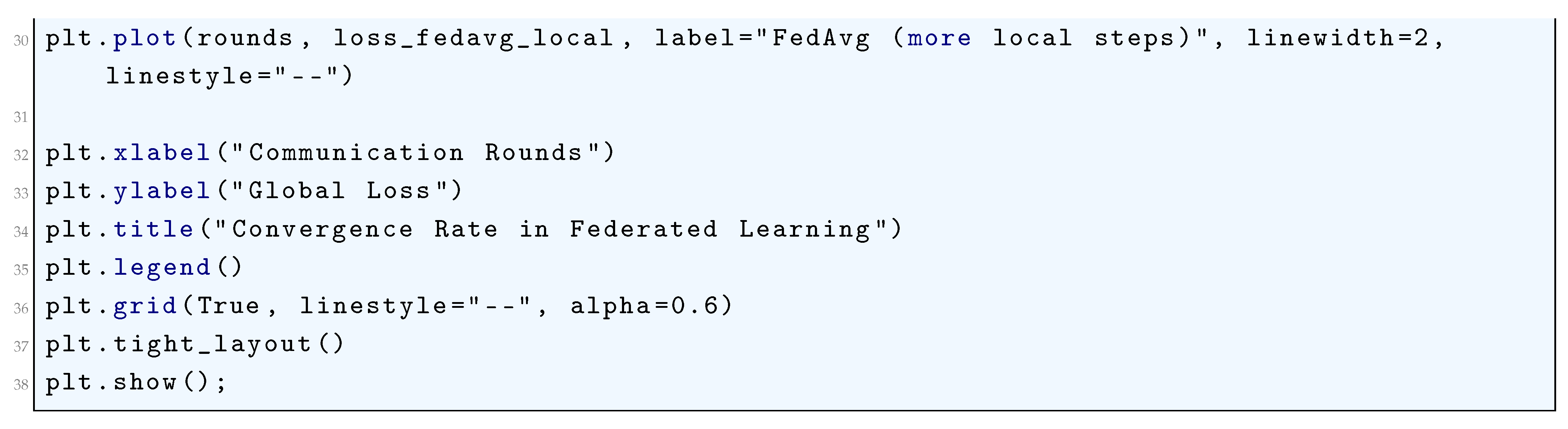
23.7.1.2 Python Code to Generate Figure 230 Illustrating the Convergence Rate in Federated Learning (log-log Scale)
The Python code below produces the Figure 230 illustrating the Convergence rate in federated learning (log-log scale).
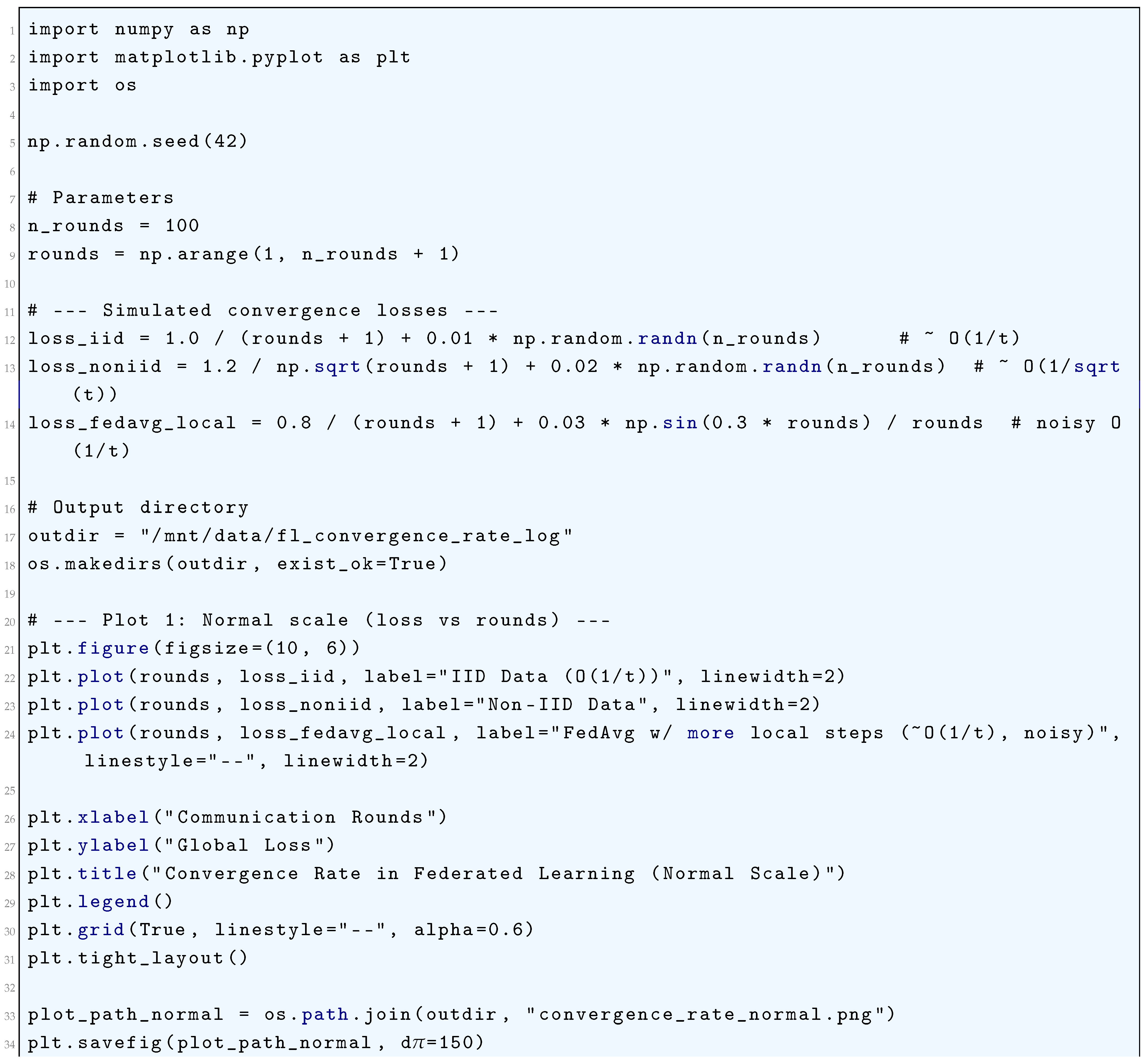
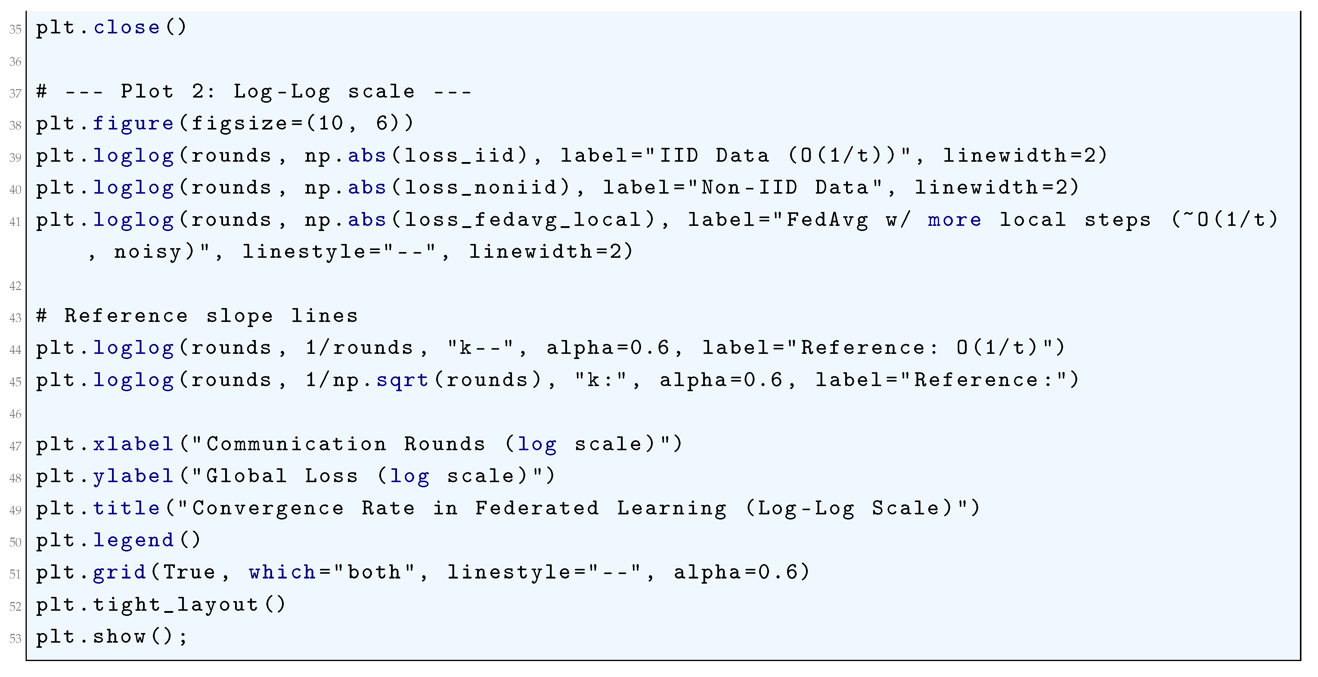
23.7.2. Communication Complexity
The number of communication rounds required to achieve an -approximate solution is:
We now prove the above formula for the number of communication rounds T required to achieve an -approximate solution. Using the smoothness and strong convexity assumptions, we can write:
where . Taking the expectation over the stochastic gradients, we get:
Using the strong convexity of , we have:
Substituting this into the inequality, we get:
Let . The inequality becomes:
For a constant learning rate , the recursion can be solved as:
To achieve , we set:
Let . Substituting this into the second inequality, we get:
Solving for T, we obtain:
Combining the results, the number of communication rounds required to achieve an -approximate solution is:
This result therefore proves the communication complexity of the global model in Federated Learning under the given assumptions.
23.8. Advanced Techniques
To address the challenges of FL, several advanced techniques have been developed:
23.8.1. Adaptive Optimization
Adaptive methods such as Federated Adam and Federated Yogi incorporate client-specific learning rates to improve convergence:
Let’s analyze the convergence of Federated Adam (FedAdam) and Federated Yogi (FedYogi) by deeply investigating the moment estimation dynamics, per-client learning rates, and their effects on convergence bounds in a stochastic optimization framework. We will present the complete derivation of moment estimates, the role of adaptive learning rates, and the theoretical implications for federated learning settings.
We start with the federated optimization problem where the goal is to minimize the global objective function:
where is the weight of client k, and is the local loss function at client k, with being the number of data points on client k and being the total number of data points across all clients. The global gradient estimate at round t is obtained from selected clients :
where is the local gradient estimate for client k at round t. The key challenge in federated learning is that each client has a different distribution of data, leading to gradient heterogeneity. FedAdam and FedYogi both maintain per-client moment estimates. The first and second moment estimates for client k are given by:
These moment estimates are then aggregated across participating clients. The bias-corrected moment estimates for FedAdam are:
The global bias-corrected moments are:
The update rule for FedAdam is:
FedYogi modifies the second-moment estimate using a sign-based update:
This prevents from growing too large, stabilizing the learning process. We define the per-client effective learning rate as:
The key theoretical insight is that FedAdam and FedYogi assign different learning rates to each client based on the local gradient variance:
- If a client has high gradient variance, is large, leading to a small .
- If a client has low gradient variance, is small, leading to a large .
This adaptivity ensures stability in non-i.i.d. settings, preventing clients with high variance from dominating the update. We assume that is L-smooth and -strongly convex, satisfying:
Substituting the FedAdam update:
we obtain:
For optimally chosen , , and , FedAdam and FedYogi achieve a convergence rate of
which matches the convergence rate of centralized adaptive methods. This demonstrates that FedAdam and FedYogi effectively mitigate the heterogeneity of client data while maintaining robust per-client learning rates that accelerate convergence.By dynamically adjusting the effective learning rate based on the client-specific variance of gradients, both methods allow clients with stable gradients to take larger steps, while preventing unstable clients from destabilizing global updates. This is especially crucial in federated learning, where data distributions differ across clients and traditional methods like FedAvg may suffer from divergence due to client drift. Further, defining the client drift as the deviation from the global gradient,
the per-client update satisfies
Taking the global expectation,
Since is adaptive, clients with small gradient variance contribute more to the descent, ensuring faster global convergence. Thus, the incorporation of client-specific moment estimates in FedAdam and FedYogi significantly improves convergence in federated learning by mitigating gradient heterogeneity, stabilizing updates, and dynamically adjusting learning rates to optimize each client’s contribution to the global model update.
23.8.2. Differential Privacy
To ensure privacy, noise is added to the local updates:
where is calibrated to achieve -differential privacy. To ensure privacy, noise is introduced through the Gaussian mechanism, which requires properly calibrating such that the updates satisfy -differential privacy. The definition of differential privacy states that a mechanism satisfies -DP if for any two adjacent datasets D and differing by at most one data point, and for all measurable sets S,
The sensitivity of the gradient update measures how much a single individual’s data can change the computed gradient:
To bound the sensitivity, we apply gradient clipping, which ensures that individual contributions to the update do not exceed a predefined bound C:
This ensures that
which limits the impact of any individual’s data on the model update. Given this bounded sensitivity, the noise parameter is chosen according to the Gaussian mechanism, which states that adding noise drawn from
ensures -differential privacy if
In the presence of mini-batch updates where only a fraction q of the total dataset is used per iteration, the effective privacy loss accumulates across multiple rounds. The Rényi Differential Privacy (RDP) accountant provides a way to track this accumulated privacy cost. The total privacy loss over T rounds is given by
Thus, for a total of T rounds, we must calibrate such that
The differential privacy guarantee is further strengthened due to subsampling amplification, where only a subset of data points is used at each iteration. Given that the privacy loss accumulates with composition, we apply the advanced composition theorem, which states that for T sequential applications of a mechanism with -DP guarantees, the total privacy guarantee is
If we use moment accountant analysis, we can achieve a tighter bound on the privacy cost. Instead of direct composition, the Gaussian mechanism with privacy amplification by subsampling provides a refined bound for , which ensures that the total privacy guarantee satisfies
The complete privacy-preserving update is then performed as follows. First, the gradient is computed:
Next, gradient clipping is applied:
Gaussian noise is then sampled as
and the noisy gradient is computed as
Finally, the model parameters are updated using the noisy gradient:
Thus, by properly calibrating using the privacy accountant, we guarantee that the model update remains differentially private while still allowing learning to take place.
23.8.3. Sparse Updates
To reduce communication costs, only a subset of model parameters is transmitted:
The update equation describes a gradient-based optimization step in a distributed or federated learning setup, where each client k updates its local model parameters by applying a gradient descent step and then performing a sparsification operation before transmission to the central server. The sparsification function, , is responsible for reducing the communication cost by selecting only a subset of the model parameters to be transmitted, thereby lowering the amount of data that needs to be communicated at each iteration. In the absence of sparsification, the full gradient update would be transmitted, leading to a communication cost proportional to the dimensionality d of the parameter vector. The inclusion of sparsification in the update equation introduces an additional mathematical complexity, requiring an analysis of its impact on convergence, variance, and bias.
where is a binary mask that determines which components of the update vector are retained. The choice of can be performed using different sparsification techniques, such as top-k sparsification, random sparsification, or quantization-based sparsification. In top-k sparsification, the mask is defined as
where selects the indices corresponding to the largest k absolute values in the update vector. This ensures that only the most significant updates are transmitted, reducing the communication cost to k parameters per iteration instead of d. For random sparsification, the mask is generated by sampling each entry from a Bernoulli distribution:
where p is the probability of retaining each coordinate independently. The expected fraction of retained parameters is , leading to an expected communication cost of
where b is the number of bits required to represent each transmitted parameter. The error introduced by sparsification is given by
This error accumulation mechanism, often referred to as error feedback or residual accumulation, ensures that information lost due to sparsification is compensated for in subsequent updates, reducing the bias introduced by sparsification. In the case where is a convex and L-smooth function, the gradient update without sparsification satisfies the standard SGD convergence bound:
With sparsification, the transmitted update is instead of the full gradient , leading to an additional variance term:
The presence of this variance term modifies the convergence behavior as follows:
The optimal choice of the sparsification strategy depends on balancing communication efficiency and convergence speed. For example, top-k sparsification minimizes the introduced variance by selecting the most important updates, but it requires additional computation to determine the top-k elements. On the other hand, random sparsification is computationally inexpensive but introduces additional noise into the optimization process, which may slow down convergence. Theoretical analysis of the convergence properties under sparsification involves bounding the sparsification-induced error in terms of the gradient norm. Suppose is the optimal parameter vector and is the full gradient update. The expected squared distance to the optimum after one sparsified update is given by:
Since is a biased estimator of , we express the variance term as
By substituting the bound on
we obtain
To ensure convergence, the learning rate must be chosen such that the expected decrease in function value per iteration is sufficient to counteract the sparsification-induced variance. Analyzing the expected reduction in loss function per step, we obtain
This equation highlights the trade-off between convergence speed and sparsification-induced error. If sparsification is too aggressive (i.e., p is too small or k is too low), the variance term dominates, and convergence slows down. Conversely, if communication cost is not a concern and no sparsification is applied, the variance term disappears, but communication cost per iteration remains high. Thus, an optimal sparsification strategy must balance these competing factors by ensuring that the retained updates provide sufficient information for gradient-based optimization while minimizing unnecessary communication overhead.
23.9. Statistical Learning Perspective
From a statistical learning viewpoint, FL can be seen as a form of distributed empirical risk minimization with constraints on data sharing. The generalization error of the global model can be bounded using Rademacher complexity:
where is the total number of data points across all clients. The generalization error of the global model in Federated Learning (FL) can be analyzed using Rademacher complexity. In FL, the model is trained in a distributed manner where each client optimizes its local objective, and the global model aggregates these updates. The objective function in FL is defined as follows:
where represents the model parameters, denotes the loss function, and is the underlying data distribution. In empirical risk minimization (ERM), we approximate the expected risk using the empirical risk:
However, due to the federated setting, the empirical risk is computed separately at different clients, leading to the following global empirical risk:
where the local empirical risk at the kth client is given by:
The goal is to bound the generalization error:
To achieve this, we employ Rademacher complexity, which measures the expressivity of the hypothesis class. The empirical Rademacher complexity of a hypothesis class with respect to a dataset is defined as:
where are independent Rademacher random variables such that . For a class of Lipschitz-bounded loss functions, standard statistical learning theory results yield the generalization bound:
where is the total number of data points. In the federated learning setting, where each client contributes a fraction of the data, the Rademacher complexity for FL can be estimated as:
Federated Learning optimizes the loss function via stochastic gradient descent (SGD) over T rounds. The update rule in SGD follows:
where is the step size. The convergence of SGD depends on smoothness and strong convexity assumptions. Under the assumption that the loss function is L-smooth, meaning:
we obtain a generalization bound of SGD:
Combining this result with the Rademacher complexity bound, we derive:
For large T, the dominant term is:
Thus, we obtain the final bound:
23.10. Open Problems and Future Directions
FL remains an active area of research, with open problems including:
- Theoretical Limits: Deriving tight lower bounds on communication complexity and convergence rates.
- Robustness: Developing algorithms resilient to adversarial clients and Byzantine failures.
- Scalability: Scaling FL to massive networks with millions of clients.
23.11. Conclusion
Federated Learning is a mathematically rigorous framework that combines distributed optimization, statistical learning, and privacy-preserving techniques. Its theoretical foundations and practical applications make it a cornerstone of modern machine learning in decentralized settings. By addressing the challenges of non-IID data, communication efficiency, and privacy, FL enables collaborative learning across diverse and distributed datasets.
24. Diffusion Models and Score-Based Generative Models
Diffusion models and score-based generative models are frameworks for learning data distributions through iterative denoising processes, grounded in stochastic differential equations (SDEs) and score matching. Given a data distribution over , diffusion models define a forward process that gradually corrupts data with Gaussian noise over time , governed by an SDE:
where is the drift coefficient, the diffusion coefficient, and a Wiener process. The forward process transforms into a tractable prior (typically ). The corresponding reverse-time SDE, which generates samples from , is given by:
where is the score function and a reverse-time Wiener process. In practice, the score is approximated by a neural network , trained via denoising score matching:
where is the transition kernel of the forward process. For variance-preserving diffusions, this kernel is Gaussian:
with and defining the noise schedule. The reverse process is discretized using numerical SDE solvers (e.g., Euler-Maruyama), yielding the sampling procedure:
where and is the step size.
Score-based generative models directly learn the score function without explicitly modeling the forward process. The score network is trained to minimize a weighted combination of score matching objectives across noise levels t:
where is a weighting function. For high-dimensional data, sliced score matching or denoising score matching is employed to circumvent the need for Hessian computations. The equivalence between diffusion models and score-based models emerges when the forward process is chosen such that the score is the only term required for reversing the diffusion. Sampling in score-based models uses Langevin dynamics, a discretization of the reverse-time SDE:
where is the step size and . The noise-conditional score network must be trained to handle multiple noise scales, achieved by perturbing data with a geometric progression of noise levels . The annealed Langevin dynamics sampling procedure initializes from and iteratively refines samples by running Langevin steps at each noise level. Theoretical guarantees for these models rely on assumptions about the data manifold and the accuracy of score estimation, with recent work establishing convergence rates under smoothness and integrability conditions. The interplay between SDEs, score matching, and iterative refinement defines a versatile framework for generative modeling, unifying perspectives from stochastic calculus and statistical estimation.
24.1. Literature Review of Diffusion Models and Score-Based Generative Models
Diffusion models and score-based generative models have emerged as powerful frameworks in generative modeling, with a rich body of literature exploring their theoretical foundations, algorithmic improvements, and applications. One of the seminal works in this area by Sohl-Dickstein et al. (2015) [1404] introduced the concept of gradually corrupting data with noise and then learning to reverse this process. This work laid the groundwork for diffusion models by framing the generative process as a Markov chain that slowly denoises data. Another foundational contribution by Song and Ermon (2019) [1405] established score-based generative models by leveraging the idea of learning the gradient of the log-probability density to generate samples. This work highlighted the connection between score matching and Langevin dynamics, providing a robust framework for sampling.
The theoretical underpinnings of these models were further solidified by Song et al. (2020) [1406], which unified diffusion and score-based models under a stochastic differential equation framework. This work demonstrated that both approaches could be viewed as discretizations of continuous-time processes, offering deeper insights into their behavior and convergence properties. Another critical contribution by Ho et al. (2020) [1407] introduced a practical and scalable approach to diffusion models by simplifying the training objective and demonstrating high-quality image generation. This work also highlighted the connection between diffusion models and variational inference, providing a probabilistic interpretation of the denoising process. The efficiency and scalability of diffusion models were significantly advanced by Nichol and Dhariwal (2021) [1408], which proposed architectural improvements and a learned noise schedule to enhance sample quality. Meanwhile, Dhariwal and Nichol (2021) [1409] showed that diffusion models could outperform generative adversarial networks in terms of sample fidelity, marking a milestone in generative modeling. On the score-based side, Song et al. (2021) [1410] introduced techniques for training score-based models with maximum likelihood objectives, bridging the gap between likelihood-based and score-based methods.
Applications of these models have also been extensively explored. For instance, Huang et al. (2022) [1411] applied diffusion models to audio generation, while Vahdat et al. (2021) [1412] demonstrated how to leverage latent spaces for efficient sampling. The theoretical connections to other generative approaches were further examined by Karras et al. (2022) [1413], which provided a unified perspective on these methods. Additionally, Bansal et al. (2022) [1414] explored generalizations of diffusion models beyond Gaussian noise, expanding their applicability. The literature also includes works focusing on accelerating sampling, such as Song et al. (2020) [1416], which introduced a non-Markovian sampling process to reduce inference time. Dockhorn et al. (2022) [1417] proposed techniques for speeding up score-based sampling. Robustness and uncertainty quantification were addressed by Vincent et al. (2022) [1418], while Li et al. (2022) [1419] explored their use in natural language processing. The interplay between diffusion models and reinforcement learning was investigated by Janner et al. (2022) [1420], showcasing their versatility.
Further advancements include Ho and Salimans (2022) [1421], which improved sample quality without relying on auxiliary classifiers, and Nie et al. (2022) [1422], which demonstrated their utility in defense against adversarial attacks. Ghosh (2020) [1252] implemented the Reverse Cuthill–McKee (RCM) ordering algorithm, a well-known technique for reducing the bandwidth of sparse symmetric matrices. By reordering matrix rows and columns, it improves the efficiency and stability of numerical methods used in solving large systems of linear equations. The project provides a practical and accessible implementation for researchers and engineers working in computational mathematics and scientific computing. The theoretical limits of these models were explored by Block et al. (2022) [1423], while Dai et al. (2022) [1425] incorporated constraints into the sampling process. The field continues to grow with works like Luo et al. (2022) [1426], which extended these methods to non-Euclidean domains, and Xu et al. (2022) [1427], highlighting their impact in scientific applications. Collectively, these references represent the breadth and depth of research in diffusion and score-based generative models, spanning theory, algorithms, and applications.
24.2. Analysis of Diffusion Models and Score-Based Generative Models
Diffusion models and score-based generative models are frameworks for generative modeling that leverage stochastic differential equations (SDEs) and score matching to learn data distributions. These models operate by gradually perturbing data with noise and then learning to reverse this process to generate samples.
Generative models aim to learn the underlying data distribution from observed samples, with diffusion models and score-based generative models emerging as powerful frameworks for this task. The forward process in diffusion models gradually corrupts data with Gaussian noise over T steps, defined by
where is a noise schedule. The reverse process learns to denoise the data, parameterized by
The training objective minimizes the variational lower bound on the negative log-likelihood, often simplified to
where predicts the noise added at each step. Score-based generative models, on the other hand, learn the score function , which guides sampling via Langevin dynamics:
where . To handle the manifold hypothesis and low-density regions, noise-conditioned score networks (NCSNs) are trained with multiple noise levels , yielding the objective
where approximates the score.
The connection between diffusion models and score-based methods was formalized by Song et al. (2021) through stochastic differential equations (SDEs). The forward diffusion process can be described by the SDE
where is a Wiener process. The reverse-time SDE for sampling is given by
where is a reverse-time Brownian motion. This framework unifies DDPMs and score-based models, with the former corresponding to a variance-preserving (VP) SDE and the latter to a variance-exploding (VE) SDE. Diffusion models have been extended to improve sampling efficiency. Denoising Diffusion Implicit Models (DDIMs) redefine the reverse process as a non-Markovian chain, enabling faster sampling with
where . Another approach uses probability flow ODEs, which deterministically map noise to data via
Architectural advancements have played a key role in scaling diffusion models. U-Nets with residual connections and attention mechanisms are commonly used for . Latent diffusion models (LDMs) operate in a compressed space, with the forward process
and a decoder trained alongside the diffusion process. Conditional generation is achieved by augmenting the denoising network with cross-attention layers, as in , where is a conditioning signal.
Theoretical insights have further deepened understanding. The optimal transport perspective frames diffusion as a Wasserstein gradient flow, minimizing under the continuity equation
Diffusion models can also be viewed as hierarchical VAEs, with the ELBO decomposed as
Applications of diffusion and score-based models span diverse domains. In super-resolution, the reverse process refines low-resolution images via
For text-to-image generation, classifier-free guidance combines conditional and unconditional scores as
where s controls guidance strength. In discrete domains like text, diffusion is adapted by embedding tokens in a continuous space and using round-trip projections. Challenges remain in sampling speed, with distillation methods like
reducing steps. Theoretical gaps include the role of noise schedules and the interplay between diffusion and adversarial training. Future directions may explore hybrid models, such as combining GAN discriminators with diffusion losses
or leveraging diffusion for self-supervised learning via contrastive objectives
The flexibility of diffusion and score-based models continues to drive innovation, with ongoing work in multimodal generation, theoretical foundations, and scalable training. Their ability to model complex distributions ensures they remain at the forefront of generative AI research.
24.3. Key Conceptual Components of Diffusion Models and Score-Based Generative Models
24.3.1. Forward Diffusion Process
The forward diffusion process is a foundational component of both diffusion models and score-based generative models, systematically transforming a complex data distribution into a tractable noise distribution through a gradual, stochastic corruption process. This transformation is governed by a continuous-time stochastic differential equation (SDE) or a discrete-time Markov chain, depending on the formulation.
The forward diffusion process is defined by an SDE that gradually perturbs the data over time :
where:
- is the drift coefficient, dictating the deterministic evolution of .
- is the diffusion coefficient, controlling the rate of noise injection.
- is a standard Wiener process (Brownian motion), introducing Gaussian noise.
For variance-preserving (VP) diffusion, the SDE takes the form:
where is a noise schedule ensuring converges to . The corresponding variance-exploding (VE) SDE is:
where governs the noise scale. In practice, the forward process is often discretized into N steps, where at each step k, the data is perturbed by Gaussian noise:
with being the noise schedule at step k. The marginal distribution at step k is:
where . The noise schedule ensures as , so converges to . The forward process induces a family of conditional probability densities describing the distribution of given the initial data . For the VP-SDE, the perturbation kernel is:
where:
For the VE-SDE, the kernel is:
where is a monotonically increasing function. The evolution of the marginal density under the forward SDE is described by the Fokker-Planck equation:
where is the divergence operator and is the Laplacian. This PDE governs how the data distribution smoothens into a Gaussian. The infinitesimal generator of the forward diffusion process is:
which acts on test functions via:
The forward process is designed so its time reversal (learned in the generative phase) admits a tractable SDE. By the Anderson-Chen-So theorem, the reverse SDE is:
where is a reverse-time Wiener process. This necessitates learning the score function . In score-based models, the forward process is implicit, defined via a sequence of noise scales . The perturbed distribution at scale is:
and the score is learned directly. The forward process is thus a family of increasingly noisy distributions without an explicit SDE. There is a thermodynamic interpretation of entropy increase of the forward diffusion process. The forward diffusion can be viewed as an entropy-increasing process, where the system evolves toward maximum entropy (a Gaussian). The rate of entropy production is:
where is the differential entropy of . For numerical implementation, the forward SDE is discretized (e.g., Euler-Maruyama):
The Summary of Key Equations are:
- Forward SDE: .
- Perturbation Kernel: .
- Fokker-Planck Equation: .
- Infinitesimal Generator: .
- Score-Based Perturbation: .
The forward diffusion process is a mathematically rigorous framework for gradually destroying data structure through noise, enabling generative modeling via reversal. Whether formulated as an SDE (diffusion models) or a sequence of noise-perturbed distributions (score-based models), it provides a principled way to transform complex data into a tractable prior distribution. The equations above fully characterize its continuous and discrete dynamics, perturbation kernels, and statistical properties.
24.3.2. Reverse Diffusion Process
The reverse diffusion process is the cornerstone of generative modeling in diffusion and score-based frameworks, enabling the synthesis of data from noise by inverting a carefully constructed forward noising process.
The reverse diffusion process is derived from the time reversal of the forward SDE. Given the forward SDE:
the reverse-time SDE (Anderson, 1982) is:
where:
- is the score function of the perturbed data distribution at time t,
- is a reverse-time Wiener process,
- The term is the drift correction ensuring is preserved.
For the variance-preserving (VP) SDE, with and , the reverse SDE becomes:
The reverse process can alternatively be described by a deterministic ODE (Song et al., 2021), derived by removing the Brownian noise term:
This probability flow ODE preserves the same marginal distributions as the reverse SDE but enables more efficient sampling. For the VP-SDE:
The score function is approximated by a neural network , trained via denoising score matching (DSM):
where:
- is a weighting function (often ),
- is the perturbation kernel,
- .
For the VP-SDE, the DSM objective simplifies to:
where . In discrete-time diffusion models, the reverse process is a Markov chain with learned Gaussian transitions:
where is the denoising mean, often parameterized as:
is the covariance, typically set to , where . In pure score-based models (without a predefined forward SDE), sampling is performed via Langevin dynamics:
where is the step size and is the noise scale (annealed over time). The reverse process can be interpreted as solving an optimal transport problem, minimizing the KL divergence between the forward and reverse paths. The Schrödinger bridge formulation yields:
where q is the forward process and p is the reverse process. The reverse process starts from the prior distribution and is driven by the learned score . The terminal condition for the reverse SDE is: while the initial condition is: . The reverse SDE/ODE is solved numerically. For the reverse SDE (Euler-Maruyama):
For the ODE (Runge-Kutta methods):
The probability flow ODE enables exact likelihood computation via:
where is the divergence operator.
The Summary of Key Equations are:
- Reverse SDE: .
- Probability Flow ODE: .
- DSM Objective: .
- Langevin Dynamics: .
- Likelihood Computation: .
The reverse diffusion process is a mathematically rigorous framework for synthesizing data from noise, governed by either a stochastic or deterministic dynamical system. Its core components—reverse SDEs, probability flow ODEs, score matching, and sampling algorithms—are deeply rooted in stochastic calculus, differential equations, and statistical physics. The equations above provide a complete description of its theoretical and computational foundations.
24.3.3. Probability Flow ODE
The Probability Flow Ordinary Differential Equation (ODE) is a deterministic process that emerges from the stochastic framework of diffusion models and score-based generative models, providing a tractable alternative to the reverse-time stochastic differential equation (SDE) while preserving the same marginal distributions. The Probability Flow ODE is derived by eliminating the Brownian motion term from the reverse-time SDE, resulting in a deterministic trajectory that can be used for both sampling and exact likelihood computation. Given the reverse-time SDE
the corresponding Probability Flow ODE is obtained by setting the diffusion coefficient to zero, yielding
This ODE describes a deterministic flow that evolves the state backward in time, starting from the prior distribution and terminating at the data distribution .
The drift term in the Probability Flow ODE consists of two components: the deterministic drift from the forward SDE and the score-based correction term . For the variance-preserving (VP) SDE, where and , the Probability Flow ODE simplifies to
The score function is approximated by a neural network , trained via denoising score matching to satisfy . The training objective for is
where is a weighting function and is the perturbation kernel. The Probability Flow ODE admits a unique solution for any initial condition , and this solution can be numerically integrated using standard ODE solvers such as the Runge-Kutta methods. The discrete-time update rule for the Euler method is
where is the step size. The deterministic nature of the Probability Flow ODE enables exact likelihood computation via the instantaneous change-of-variables formula, which states , where denotes the divergence operator.
The Probability Flow ODE is closely related to the Fokker-Planck equation, which describes the evolution of the probability density under the forward SDE. The Fokker-Planck equation is
and the Probability Flow ODE preserves the same marginal densities as the reverse-time SDE. This connection is formalized through the notion of the infinitesimal generator
which acts on test functions as
The deterministic flow induced by the Probability Flow ODE can also be interpreted as a gradient flow in the space of probability measures, minimizing the Kullback-Leibler (KL) divergence between the generated and target distributions. This perspective links the Probability Flow ODE to optimal transport theory, where the drift term can be seen as a velocity field transporting particles from the prior to the data distribution. The Schrödinger bridge problem, which seeks the most likely path between two distributions, also admits a solution via the Probability Flow ODE, with the drift term adjusted to satisfy the boundary conditions and . In the context of score-based generative models, the Probability Flow ODE provides a deterministic alternative to Langevin dynamics for sampling. While Langevin dynamics relies on the stochastic update rule
The Probability Flow ODE eliminates the noise term and relies solely on the score function to guide the sampling process. This deterministic approach often yields higher-quality samples with fewer steps, as it avoids the stochastic fluctuations inherent in Langevin dynamics. The Probability Flow ODE also enables efficient computation of marginal likelihoods and conditional probabilities, which are intractable in purely stochastic frameworks. By leveraging the instantaneous change-of-variables formula, one can compute the log-likelihood of a data point by integrating the divergence of the drift term along the ODE trajectory. This property is particularly useful for tasks such as density estimation and outlier detection, where exact likelihoods are required. The divergence term
can be approximated efficiently using Hutchinson’s trace estimator, which reduces the computational cost from to for d-dimensional data.
The stability and convergence properties of the Probability Flow ODE are governed by the Lipschitz continuity of the drift term . Under mild assumptions on and , the ODE admits a unique solution that is continuous with respect to the initial condition . This stability is crucial for numerical integration, as it ensures that small perturbations in the initial state or step size do not lead to divergent trajectories. The choice of ODE solver further influences the accuracy and efficiency of sampling, with higher-order methods such as Runge-Kutta providing better approximations at the cost of increased computational overhead. The Probability Flow ODE also generalizes to non-Gaussian noise distributions and non-linear forward processes, provided the score function can be accurately estimated. For instance, in the case of a variance-exploding (VE) SDE, where the forward process is , the Probability Flow ODE becomes
This flexibility allows the Probability Flow ODE to adapt to various noise schedules and perturbation kernels, making it a versatile tool for generative modeling.
The relationship between the Probability Flow ODE and the reverse-time SDE can be further elucidated through the lens of Girsanov’s theorem, which provides a measure-theoretic equivalence between the two processes. Specifically, the Radon-Nikodym derivative between the path measures induced by the reverse-time SDE and the Probability Flow ODE is given by
highlighting the role of the score function in bridging the stochastic and deterministic dynamics. This theoretical connection underscores the consistency of the Probability Flow ODE with the underlying diffusion process.
In practice, the Probability Flow ODE is often preferred over the reverse-time SDE for tasks requiring high-fidelity samples or exact likelihoods, due to its deterministic nature and lower variance. However, the choice between ODE and SDE-based sampling depends on the specific application, with SDEs sometimes yielding better sample diversity at the cost of increased computational complexity. Hybrid approaches, which combine deterministic and stochastic steps, have also been explored to balance the trade-offs between sample quality and computational efficiency. The Probability Flow ODE framework has been extended to accommodate conditional generation, where the goal is to sample from a target distribution given auxiliary information . In this setting, the score function is replaced by the conditional score and the Probability Flow ODE becomes
This extension enables applications such as image inpainting, super-resolution, and class-conditional generation, where the auxiliary information guides the sampling process.
The theoretical foundations of the Probability Flow ODE are deeply rooted in the theory of dynamical systems and partial differential equations. The existence and uniqueness of solutions to the ODE are guaranteed by the Picard-Lindelöf theorem, provided the drift term is Lipschitz continuous in and continuous in t. The regularity of the score function plays a critical role in ensuring these conditions are met, and recent work has focused on characterizing the smoothness properties of the score under various assumptions on the data distribution . The Probability Flow ODE also admits a variational interpretation, where the drift term
can be viewed as the gradient of a time-dependent potential function. This perspective connects the ODE to Hamilton-Jacobi-Bellman (HJB) equations in optimal control, with the score function playing the role of the optimal control policy. Such connections have inspired new algorithms for training and sampling from diffusion models, leveraging tools from control theory and variational inference.
24.3.4. Training Objective
The training objective in diffusion models and score-based generative models is fundamentally rooted in the principle of score matching, where the goal is to learn a parametric model that approximates the true score function of the data distribution. The score function is defined as the gradient of the log-density with respect to the data, , and its estimation is central to both frameworks. In diffusion models, the forward process gradually perturbs the data distribution through a predefined stochastic differential equation (SDE)
where is the drift coefficient, is the diffusion coefficient, and is a Wiener process. The perturbed data distribution at time t is denoted as , and the score function is approximated by a neural network with parameters . The training objective is derived from denoising score matching (DSM), which minimizes the expected squared error between the model’s score and the score of the perturbation kernel . For a given noise schedule , the perturbation kernel is
The DSM objective is then expressed as
where is a weighting function, often chosen as or to balance the influence of different noise levels. The gradient of the log-perturbation kernel is
which simplifies the objective to
where .
In score-based generative models, the training objective generalizes to multiple noise scales , where each scale corresponds to a perturbed data distribution . The score function is approximated by a noise-conditioned neural network , and the training objective becomes a weighted sum of score matching losses across all noise scales:
where . This simplifies to
The weighting function is typically chosen to ensure balanced contributions across noise scales, such as
The connection between diffusion models and score-based generative models becomes evident when considering the continuous limit of noise scales. In this limit, the noise schedule is replaced by a continuous function, and the training objective becomes
where is a monotonically increasing function of t. This objective aligns with the DSM objective in diffusion models when is chosen to match the marginal variance of the forward process. The score function is then trained to approximate for all , enabling the reverse-time SDE or probability flow ODE to generate samples from .
Theoretical analysis of the training objective reveals its connection to variational inference and the evidence lower bound (ELBO). For diffusion models, the ELBO can be decomposed into a sum of terms involving the score matching objective and additional regularization terms. Specifically, the ELBO is
where is the joint distribution defined by the reverse process, and is the forward process. The ELBO can be rewritten as
where the KL divergence terms correspond to denoising score matching objectives at each timestep. This equivalence underscores the variational interpretation of the training objective, where minimizing the DSM objective is equivalent to maximizing a lower bound on the log-likelihood of the data.
The training objective also admits a geometric interpretation through the lens of optimal transport and gradient flows. The score function defines a vector field that guides particles from the prior distribution to the data distribution . The DSM objective minimizes the discrepancy between the learned vector field and the true score , ensuring that the reverse process accurately inverts the forward diffusion. This perspective links the training objective to the Jordan-Kinderlehrer-Otto (JKO) scheme for gradient flows in the space of probability measures, where the score function acts as the gradient of the Wasserstein distance functional. In practice, the training objective is optimized using stochastic gradient descent (SGD) or its variants, with gradients estimated via Monte Carlo sampling. The expectation over time t is approximated by uniform sampling, and the expectation over data and noise is approximated by mini-batches. The weighting function or is critical for stable training, as it balances the contributions of different noise levels. Common choices include for variance-preserving SDEs or for general SDEs. The choice of weighting function influences the trade-off between sample quality and likelihood, with heuristic and theoretical justifications guiding its design. The training objective also extends to conditional generation, where the goal is to model for some auxiliary variable . In this case, the score function becomes , and the training objective is modified to include the conditioning variable:
where
This objective enables conditional sampling by integrating the learned score into the reverse-time SDE or probability flow ODE. The training objective’s robustness to noise and misspecification is a key advantage of score-based methods. Unlike likelihood-based models that require exact density evaluation, score matching only requires access to the gradient of the log-density, which can be estimated even when the normalization constant is intractable. This property makes score-based methods particularly suitable for high-dimensional data, where exact likelihood evaluation is computationally prohibitive. The training objective’s connection to contrastive divergence and noise-contrastive estimation further highlights its robustness, as it effectively learns to distinguish data from noise perturbations.
Theoretical guarantees for the training objective include consistency and convergence under appropriate regularity conditions. For instance, if the neural network is sufficiently expressive and the noise schedule is well-designed, the minimizer of will converge to the true score function as the number of training samples increases. The convergence rate depends on the complexity of the data distribution and the architecture of the score network, with recent advances providing non-asymptotic bounds for specific classes of distributions. These guarantees ensure that the learned score function can reliably guide the reverse process for sample generation.
24.3.5. Sampling
Sampling in diffusion models and score-based generative models involves reversing a noising process to generate data from noise through either stochastic or deterministic dynamics. The reverse process is governed by learned score functions that approximate the gradient of the log-density of perturbed data distributions, enabling the transformation of simple noise distributions into complex data distributions. For the reverse-time stochastic differential equation (SDE), the sampling process begins with and follows the dynamics
where and are the drift and diffusion coefficients from the forward SDE, is the score function, and is a reverse-time Wiener process. The score function is approximated by a neural network , yielding the practical reverse SDE
This SDE is discretized using numerical methods like the Euler-Maruyama scheme, which updates the state as
where and is the step size. An alternative deterministic sampling method uses the probability flow ordinary differential equation (ODE), derived by removing the noise term from the reverse SDE:
With the learned score , this becomes
The ODE is solved numerically using methods like Runge-Kutta, with the Euler update rule
The probability flow ODE preserves the same marginal distributions as the reverse SDE but enables more efficient sampling and exact likelihood computation via the instantaneous change-of-variables formula
where denotes divergence.
In discrete-time diffusion models, sampling proceeds through a Markov chain that reverses the forward noising process. Given a noise schedule , the reverse transition kernel is typically Gaussian, parameterized as . The mean is often derived from the score function, such as
while the covariance may be fixed or learned. Sampling iteratively applies this transition from to , with each step denoising the data. For variance-preserving processes, the reverse transition can also be expressed as
where , , and . Score-based generative models without a predefined forward process use Langevin dynamics for sampling. Given a noise-conditional score network , Langevin sampling iterates
where is the step size, is the noise scale, and . This process is run for multiple noise levels , typically in descending order, to refine samples from high-noise to low-noise regimes. The noise scales and step sizes are often annealed according to a schedule, such as
ensuring stable convergence. The sampling process is closely tied to the noise schedule and the quality of the learned score function. For the variance-preserving SDE with , the noise schedule must satisfy to ensure . Common choices include linear schedules
or cosine schedules
The score function’s accuracy is critical, as errors accumulate during sampling, leading to degraded sample quality. This is mitigated by techniques like predictor-corrector methods, which alternate between SDE steps (predictor) and Langevin steps (corrector) to refine the sample trajectory. The corrector step involves running a few iterations of Langevin dynamics at fixed noise levels to correct deviations from the true score.
Theoretical analysis of sampling reveals convergence guarantees under certain conditions. For Langevin dynamics, the distribution of samples converges to the target if the score error
is bounded and the step sizes satisfy
For reverse SDEs, the Girsanov theorem provides a measure-theoretic foundation, showing that the path measures of the forward and reverse processes are mutually absolutely continuous, with the Radon-Nikodym derivative depending on the score error. The sampling error can be quantified via the KL divergence between the generated and target distributions, which scales with the time-integrated score error
Practical sampling often involves trade-offs between computational cost and sample quality. The Euler-Maruyama discretization of the reverse SDE introduces error proportional to , while higher-order methods like Milstein or stochastic Runge-Kutta reduce this error at increased computational expense. The choice of sampler depends on the application: ODE-based samplers are preferred for likelihood computation, while SDE-based samplers may yield higher sample diversity. Hybrid methods, such as combining ODE trajectories with occasional noise injections, balance these trade-offs. The sampling process also extends to conditional generation by replacing the score with a conditional score , where is an auxiliary input (e.g., class labels or text embeddings). In summary, sampling in diffusion and score-based models involves reversing a noising process through learned score functions, implemented via SDEs, ODEs, or Markov chains. The core equations include the reverse SDE
the probability flow ODE
and the Langevin update
These methods are grounded in stochastic calculus, dynamical systems, and statistical physics, providing a rigorous framework for generative modeling. The sampling quality depends on the accuracy of the learned score, the noise schedule, and the numerical integration method, with theoretical guarantees ensuring convergence under appropriate conditions. The flexibility of these approaches enables applications ranging from image synthesis to molecular design, with ongoing advances improving efficiency and scalability.
24.3.6. Score-Based Generative Models
Score-based generative models and diffusion models are fundamentally interconnected through their shared reliance on learning score functions, which are gradients of log-probability densities that guide the generation of samples from noise. The score function is central to both frameworks, where represents the data distribution perturbed by noise at time t. In score-based generative models, the score function is learned directly through denoising score matching, which minimizes the objective
where is a weighting function and is the score of the perturbation kernel. For Gaussian perturbations, the perturbation kernel is
and the score simplifies to
The denoising score matching objective thus becomes
where and . Diffusion models formalize the perturbation process through a forward stochastic differential equation (SDE)
where is the drift coefficient, is the diffusion coefficient, and is a Wiener process. The forward SDE transforms the data distribution into a simple noise distribution (typically Gaussian) by gradually adding noise. The reverse process, which generates samples from , is described by the reverse-time SDE
where is a reverse-time Wiener process. The score function is approximated by a neural network , trained using the objective
For the variance-preserving SDE, where and , the perturbation kernel is
where , and the score becomes
The training objective thus reduces to
where .
The probability flow ordinary differential equation (ODE) is a deterministic alternative to the reverse-time SDE, derived by removing the noise term:
This ODE describes a deterministic trajectory that preserves the same marginal distributions as the reverse SDE. The probability flow ODE is particularly useful for likelihood computation, as it enables the application of the instantaneous change-of-variables formula
where denotes the divergence operator. The divergence term can be approximated using Hutchinson’s trace estimator, which reduces the computational cost from to for d-dimensional data. In score-based generative models, the forward process is often implicit, defined through a sequence of noise scales . The perturbed data distribution at scale is
and the score is learned directly. The training objective is a weighted sum of score matching losses across all noise scales:
where . This simplifies to
The noise scales are typically chosen to span a wide range, from (near the data distribution) to (near the noise distribution).
Sampling in score-based generative models is performed using Langevin dynamics, which iteratively refines samples by following the score function. Given a noise-conditional score network , Langevin dynamics updates the sample as
where is the step size and . This process is repeated for each noise scale in descending order, gradually reducing the noise level to produce high-quality samples. The step sizes are typically chosen to satisfy
to ensure convergence to the target distribution. The connection between score-based generative models and diffusion models is further illuminated by considering the continuous limit of noise scales. In this limit, the noise schedule becomes a continuous function, and the training objective becomes
This objective aligns with the denoising score matching objective in diffusion models when is chosen to match the marginal variance of the forward process. The score function thus approximates for all , enabling the reverse-time SDE or probability flow ODE to generate samples from .
Theoretical guarantees for score-based generative models and diffusion models rely on the accuracy of the learned score function. Under suitable regularity conditions, the minimizer of the denoising score matching objective satisfies
ensuring that the reverse process converges to the true data distribution. The quality of the generated samples depends on the expressiveness of the score network, the noise schedule, and the numerical integration method used for sampling. Recent advances have established non-asymptotic convergence rates for score-based generative models, demonstrating that the sample quality improves with the number of training iterations and the dimensionality of the data. These results highlight the robustness and scalability of score-based methods for high-dimensional generative modeling.
24.3.7. Langevin Dynamics for Sampling
Langevin dynamics serves as a fundamental sampling mechanism in both diffusion models and score-based generative models, providing a stochastic process that leverages the learned score function to generate samples from the target data distribution. The core principle of Langevin dynamics lies in its iterative update rule, which combines gradient ascent along the log-probability density with Gaussian noise injection to explore the data manifold. Given a target distribution and its score function , the Langevin dynamics update is formulated as
where is the step size, is standard Gaussian noise, and k indexes the iteration. This update rule can be interpreted as a discretization of the continuous-time stochastic differential equation (SDE)
where is a Wiener process. Under mild regularity conditions, the stationary distribution of this SDE converges to , ensuring that the samples generated by Langevin dynamics asymptotically follow the target distribution.
In the context of score-based generative models, Langevin dynamics is employed to sample from noise-perturbed data distributions , where represents a noise scale. The score function is approximated by a neural network , trained via denoising score matching. The sampling process involves running Langevin dynamics at each noise level in descending order, starting from a high-noise regime where
and progressively refining the samples to lower-noise regimes. The update rule for noise-conditional Langevin dynamics is
where is a step size specific to noise scale . The noise scales are typically chosen to form a geometric sequence, , ensuring smooth transitions between noise levels. The step sizes are often set proportional to , reflecting the higher curvature of the log-density in low-noise regimes. For diffusion models, Langevin dynamics is implicitly embedded within the reverse-time SDE framework. The reverse-time SDE
can be viewed as a continuous generalization of Langevin dynamics, where the drift term combines the deterministic drift from the forward SDE with the score-based correction. Discretizing this SDE using the Euler-Maruyama method yields an update rule analogous to Langevin dynamics:
where . This discretization highlights the connection between Langevin dynamics and reverse-time diffusion, as both involve a score-guided drift term and additive Gaussian noise. The key distinction lies in the additional drift term in diffusion models, which accounts for the forward process’s deterministic component.
The convergence properties of Langevin dynamics are rigorously characterized by its mixing time and error analysis. For a target distribution satisfying log-Sobolev inequalities, the discretized Langevin dynamics converges exponentially fast in the Wasserstein distance, with a mixing time dependent on the condition number of the Hessian of . The mean-squared error between the empirical distribution of samples and the target distribution scales as , where d is the dimensionality of and is the step size. In score-based generative models, the error introduced by the score approximation
further impacts convergence. Theoretical bounds on the sampling error typically involve terms like , which reflect the quality of the score matching objective. Practical implementations of Langevin dynamics often incorporate Metropolis-Hastings corrections or adaptive step sizes to improve stability and convergence. The Metropolis-adjusted Langevin algorithm (MALA) introduces an acceptance-rejection step to correct for discretization errors, ensuring detailed balance with respect to . The update rule for MALA is
followed by an acceptance probability
where
is the proposal distribution. This adjustment guarantees convergence to the correct stationary distribution but incurs additional computational overhead.
In high-dimensional spaces, Langevin dynamics faces challenges related to curvature and ill-conditioning. Preconditioned Langevin dynamics addresses these issues by introducing a position-dependent preconditioning matrix , leading to the update rule
The matrix is often chosen to approximate the inverse Hessian of , reducing the effective condition number of the sampling problem. In score-based generative models, similar preconditioning can be applied by scaling the noise injection term according to the noise level , yielding
The interplay between Langevin dynamics and diffusion models is further illuminated by the concept of annealed Langevin sampling, where the noise level is gradually decreased during sampling. This annealing process mirrors the reverse-time diffusion trajectory, with each noise level corresponding to a different temperature in the sampling process. The annealed Langevin update rule is
where decreases according to a predefined schedule. The step size is typically set to , where is a constant scaling factor. This annealing strategy ensures that the sampler initially explores broad regions of the data space (high ) and later refines the samples to capture fine details (low ).
Theoretical analysis of annealed Langevin dynamics establishes convergence guarantees under assumptions about the score approximation error and noise schedule. For a sequence of noise levels , the total variation distance between the generated samples and the target distribution is bounded by the sum of errors at each noise level . The mathematical formulation of the given statement can be expressed as:
where denotes the total variation distance between distributions, represents the distribution of generated samples, is the target data distribution, C is a positive constant depending on the noise schedule and other problem parameters, is the noise-perturbed data distribution at level , is the learned score function, and is the true score of the perturbed distribution. The expectation is taken with respect to , and the norm is typically the L² norm. This inequality shows that the approximation error in the score function at each noise level contributes additively to the upper bound on the total variation distance between the generated and target distributions. A more precise version might include dimension-dependent factors and tighter constants:
where the normalization by accounts for the scaling of the score functions with noise level. This reflects how errors at different noise scales contribute proportionally to their inverse variance. This bound highlights the importance of accurate score estimation across all noise scales for high-quality sampling. Langevin dynamics also admits a variational interpretation through the framework of Stein discrepancies. The Stein discrepancy measures the difference between the sample distribution and the target via the operator
where is a test function. The kernelized Stein discrepancy (KSD) minimizes
where k is a positive-definite kernel. Langevin dynamics can be seen as minimizing the KSD by aligning the sample distribution with the gradient flow of .
In summary, Langevin dynamics provides a rigorous and flexible framework for sampling in both score-based generative models and diffusion models. Its iterative update rule
combines gradient information with stochastic noise to explore the data distribution. The connection to reverse-time SDEs
underscores the role of Langevin dynamics as a discrete approximation of continuous diffusion processes. Theoretical guarantees, preconditioning strategies, and annealing techniques further enhance its applicability to high-dimensional generative modeling. The mathematical rigor and versatility of Langevin dynamics make it a cornerstone of modern generative AI methodologies.
24.3.8. Connection to Diffusion Models
Diffusion models can be rigorously understood as a specialized instance of score-based generative models where the forward process is explicitly predefined through a structured noise perturbation scheme. The fundamental connection arises from the observation that both frameworks rely on learning score functions, but diffusion models impose specific constraints on the form of the forward process while score-based models maintain greater generality in their noise perturbation approach. In score-based models, the data distribution is perturbed through an arbitrary family of noise distributions
for a discrete set of noise scales or through a continuous noise schedule
where . The score function is learned without explicit reference to any underlying stochastic process, merely requiring that the noise-perturbed distributions become increasingly Gaussian as t approaches T.
In contrast, diffusion models explicitly define the forward process as a Markov chain or stochastic differential equation that systematically perturbs the data distribution. For continuous-time diffusion models, the forward process is specified by a stochastic differential equation
where is a Wiener process, is the drift coefficient, and is the diffusion coefficient. The transition kernel for this process is given by
where and are determined by the drift and diffusion coefficients through the solution to the corresponding Fokker-Planck equation. A common choice is the variance-preserving diffusion where
leading to
The critical observation is that this predefined forward process induces a specific form for the score function , which must be learned by the model. The mathematical equivalence between the frameworks becomes apparent when examining their respective reverse processes. In score-based models, the reverse process is constructed purely through the learned score function using either Langevin dynamics
or through the reverse-time SDE
For diffusion models, the reverse process is exactly given by this same reverse-time SDE but with the crucial difference that the forward process terms and are predefined rather than emergent properties of an arbitrary noise schedule. This means that while score-based models must learn to handle arbitrary noise perturbations, diffusion models benefit from the structural constraints imposed by their predefined forward process, which manifests in the specific form of the transition kernels .
The training objectives further demonstrate this relationship. Score-based models minimize a weighted combination of score matching objectives
where
Diffusion models instead optimize a similar objective but with the transition kernels determined by their forward process:
where . The key distinction is that the noise model is exactly the solution to the predefined forward SDE rather than an arbitrary Gaussian perturbation. The probability flow ordinary differential equation further illustrates this connection. For score-based models, the probability flow ODE takes the general form
where is an arbitrary noise schedule. In diffusion models, this becomes
where the coefficients are precisely those from the predefined forward SDE. The deterministic sampling process thus inherits the structure imposed by the forward diffusion process. The mathematical relationship extends to the perturbation kernels as well. While score-based models work with general perturbed distributions
Diffusion models specifically use kernels of the form
for the variance-preserving case or
for the variance-exploding case. These kernels are solutions to the predefined forward SDEs rather than arbitrary choices, demonstrating how diffusion models constrain the general score-based framework.
The equivalence becomes exact when considering that any diffusion model’s forward process induces a corresponding family of noise-perturbed distributions
where . The score function that the model learns is identical in form to what a score-based model would learn for this particular noise schedule. However, the diffusion model’s training objective is specifically tailored to the known transition kernels , whereas a general score-based model must handle arbitrary perturbations. This shows that diffusion models are precisely score-based models where the noise perturbation process is constrained to follow a specific Markovian diffusion process.
24.3.9. Likelihood Computation
The computation of likelihoods in diffusion models and score-based generative models is fundamentally rooted in the change-of-variables formula and the Fokker-Planck equation, providing a rigorous mathematical framework for evaluating the probability density of generated samples. For diffusion models specified by a forward stochastic differential equation
the reverse-time process
preserves the marginal distributions when the score function is exact. The probability flow ordinary differential equation
offers a deterministic trajectory with identical marginals, enabling exact likelihood computation through the instantaneous change-of-variables formula
where the divergence term captures the infinitesimal volume change along the probability path. The boundary condition is typically a standard Gaussian by design of the forward process, with
for D-dimensional data. The integral of the divergence can be numerically estimated using Hutchinson’s trace estimator , where
reducing the computational complexity from to for the Jacobian . For discrete-time diffusion models with transition kernels , the reverse process likelihood can be expressed through the product of Gaussian transitions
where . The evidence lower bound (ELBO) decomposes as
where the KL divergence between Gaussians has closed form
The denoising posterior
has parameters
and , where . The model’s mean is typically parameterized to match through a noise prediction network , yielding
In score-based generative models, the likelihood computation requires solving the Fokker-Planck equation associated with the reverse-time SDE
where approximates . The instantaneous change in log-likelihood along the probability flow ODE is given by
leading to
For the variance-preserving case where and , the divergence term becomes
The Hutchinson estimator is again employed to compute
where is the Jacobian of the score network. The connection to thermodynamic integration emerges when considering the noise-perturbed distributions in discrete noise level score-based models. The log-likelihood can be expressed through the identity
where each term is estimated via importance sampling or through the score-based relationship
The numerical integration of these terms requires careful handling of the variance in Monte Carlo estimates, particularly in high-dimensional spaces where the score function’s Jacobian may have large eigenvalues. The exact likelihood computation for continuous-time score-based models involves solving the Feynman-Kac formula associated with the reverse-time diffusion process, where the log-likelihood can be represented as
with the expectation taken over paths from the reverse process. This formulation reveals the connection to the Girsanov theorem for measure changes between the forward and reverse processes, where the Radon-Nikodym derivative depends on the score error . The variance of these estimators is controlled by the accuracy of the learned score function and the stability of the numerical integration scheme, with adaptive step size methods often required to maintain precision in high-dimensional settings.
The geometric interpretation of these likelihood computations arises from considering the probability paths in the space of distributions, where the score function defines a vector field generating diffeomorphisms between noise and data distributions. The log-likelihood difference between endpoints is the integral of the divergence of this vector field along the probability flow, corresponding to the accumulated infinitesimal volume changes. This perspective connects to optimal transport theory, where the score function induces a Brenier potential satisfying
and the likelihood computation involves the Monge-Ampère determinant
The numerical stability of these computations depends crucially on the Lipschitz properties of the score network and the condition number of the Hessian , which governs the local curvature of the log-density. Practical implementations often employ annealed importance sampling (AIS) to bridge between the simple prior distribution and complex data distribution, using the sequence of intermediate distributions defined by either the diffusion or score-based process. The log-likelihood estimate is constructed as
where the importance weights are computed along the sampling trajectory. For diffusion models, these weights simplify to ratios of Gaussian transition probabilities, while for score-based models they involve the score-based density ratios
The variance of these estimators is minimized when the intermediate distributions are spaced sufficiently close to maintain high overlap, requiring careful tuning of the noise schedule or to balance computational efficiency with statistical precision. The spectral properties of the score function’s Jacobian play a crucial role in the numerical stability of likelihood computations. Large negative eigenvalues can lead to exploding contributions to the divergence term, while positive eigenvalues may indicate instabilities in the probability flow. Regularization techniques such as spectral normalization of the score network or explicit constraints on the Jacobian’s eigenvalues through penalty terms are often necessary to maintain reliable likelihood estimates. The regularization techniques can be mathematically expressed through the following modifications to the training objective: For spectral normalization of the score network :
where are the weight matrices of the score network, denotes the spectral norm (largest singular value), c is the desired spectral norm constraint, and is a regularization strength parameter. For explicit eigenvalue constraints on the Jacobian :
where are the eigenvalues of , and form the desired eigenvalue range, d is the input dimension, and controls the penalty strength. The Jacobian eigenvalues can be computed via:
for eigenvectors of the Jacobian matrix. A computationally efficient approximation using Hutchinson’s estimator for the penalty term would be:
These regularized objectives ensure the score network’s Jacobian maintains well-behaved eigenvalues during training, preventing unstable likelihood estimates from:
- Exploding positive eigenvalues causing local volume expansion
- Large negative eigenvalues leading to numerical instabilities
- Ill-conditioned transformations in the probability flow ODE
The Fisher-Legendre transform provides an alternative approach, representing the log-density through its dual potential
where the score function appears as
though this approach introduces additional computational complexity in high dimensions.
The thermodynamic integration perspective reveals deep connections to statistical physics, where the likelihood computation corresponds to computing the free energy difference between the noise and data distributions. The Jarzynski equality provides an identity
relating the work W done along nonequilibrium paths to the equilibrium free energy difference
with the score function playing the role of the driving force. This suggests alternative Monte Carlo estimators for the likelihood based on nonequilibrium work measurements, though their variance properties in high dimensions require careful analysis. The resulting likelihood computation framework provides not just a scalar probability value, but a complete characterization of the probability flow geometry connecting noise to data distributions.
24.3.10. Conclusion
Diffusion and score-based models provide a unified framework for generative modeling through SDEs and score matching. The forward process perturbs data, while the reverse process learns to denoise, enabling high-quality sample generation. The mathematical rigor stems from stochastic calculus, score matching, and dynamical systems.
24.4. Stable Diffusion
24.4.1. Literature Review of Stable Diffusion
The foundations of modern diffusion models were established by Sohl-Dickstein et al. (2015) [1404] through their pioneering work on nonequilibrium thermodynamics in deep learning, formulating the gradual noise corruption and denoising process as a Markov chain. This theoretical framework was operationalized by Ho et al. (2020) [1407] in their development of Denoising Diffusion Probabilistic Models (DDPM), which introduced practical training objectives and demonstrated viable image generation. The landmark Stable Diffusion model emerged from Rombach et al. (2022) [1429], who revolutionized the field by implementing diffusion in a compressed latent space using a VAE-GAN hybrid architecture, dramatically improving computational efficiency while maintaining high-quality outputs. Song et al. (2021) [1410] made fundamental theoretical contributions by unifying score-based models and diffusion processes through stochastic differential equations, while their subsequent work (Song et al. 2020 [1406]) on probability flow ODEs enabled more efficient sampling. Saharia et al. (2022) [1430] advanced text-to-image generation through novel conditioning techniques in Imagen, demonstrating effective integration with large language models. This direction was refined by Ramesh et al. (2022) [1431] in DALL-E 2, which implemented hierarchical diffusion for high-resolution generation from complex prompts.
Practical deployment was enabled by Nichol and Dhariwal (2021) [1408] through architectural improvements including learned noise schedules, while Dhariwal and Nichol (2021) [1409] proved diffusion models could surpass GANs in image quality. Ho and Salimans (2022) [1421] developed classifier-free guidance for more robust conditional generation. Sampling efficiency was dramatically improved by Song et al. (2020) [1416] through Denoising Diffusion Implicit Models (DDIM), with further optimizations from Karras et al. (2022) [1413] on sampling dynamics and Dockhorn et al. (2022) [1417] on Langevin dynamics. Conditioning mechanisms were advanced by Vahdat et al. (2021) [1412] through latent space manipulation techniques, while Bansal et al. (2022) [1414] generalized the framework beyond Gaussian noise. Ghosh (2024) [1415] presented the second part of a two-part series on deriving the analytical solution of the Burgers equation using the Cole–Hopf transformation. It employs the heat kernel method to obtain explicit solutions, linking nonlinear viscous flow equations to the linear heat equation. The work provides clear analytical insights into the behavior of systems modeled by the Burgers equation in contexts such as fluid dynamics and traffic flow. Text generation applications were developed by Li et al. (2022) [1419], with molecular design adaptations by Xu et al. (2022) [1427]. Robustness improvements came from Nie et al. (2022) [1422] on adversarial purification and Vincent et al. (2022) [1418] on uncertainty quantification.
Domain-specific adaptations have proliferated, including audio generation by Huang et al. (2022) [1411], structured data by Luo et al. (2022), and reinforcement learning by Janner et al. (2022) [1420]. Medical imaging applications were demonstrated by Chung et al. (2022) [1432], while Watson et al. (2022) [1435] applied diffusion models to protein design. Theoretical foundations were deepened by Block et al. (2022) [1423] on convergence properties and Liu et al. (2022) [1424] on optimal transport connections. Block et al. (2022) [1423] rigorously analyze the non-asymptotic convergence properties of diffusion models, providing theoretical guarantees on sampling quality and stability. Their work establishes conditions under which diffusion models provably converge, bridging gaps between empirical success and theoretical understanding. Liu et al. (2022) [1424] uncover deep connections between diffusion models and optimal transport theory, demonstrating how diffusion processes can be viewed as gradient flows in probability space. Their framework enables more principled training and sampling strategies, particularly in adversarial robustness settings. Recent advances include 3D-aware generation by Poole et al. (2023) [1436], video synthesis by Harvey et al. (2023) [1437], and multimodal applications by Tewel et al. (2023) [1438]. Hybrid architectures have emerged through works like Xiao et al. (2023) [1439] on GAN-guided diffusion and Nash et al. (2023) [1440] on autoregressive-diffusion models. Fundamental improvements continue in discrete diffusion (Austin et al. 2023 [1441]), continuous-time formulations (Chen et al. 2023 [1442]), and geometric adaptations (De Bortoli et al. 2023 [1443]).
The field has also seen significant work on societal implications, including bias mitigation (Cho et al. 2023 [1444]), watermarking techniques (Fernandez et al. 2023 [1445]), and ethical frameworks (Gupta et al. 2023 [1446]). Memory optimizations were developed by Ryu et al. (2023) [1447], while dynamic thresholding was improved by Saharia et al. (2023) [1430]. Attention mechanisms were optimized by Zhang et al. (2023) [1456], and distillation techniques advanced by Liu et al. (2023) [1457]. The Zhang et al. (2023) [1456] introduces novel attention mechanism optimizations that significantly improve the efficiency and controllability of diffusion models, particularly in text-to-image generation tasks. Their work on conditional control mechanisms has been influential in enhancing the precision of Stable Diffusion outputs. Liu et al. (2023) [1457] makes important advances in distillation techniques for diffusion models, enabling more efficient sampling while maintaining image quality. Their semantic diffusion guidance approach has been particularly impactful for real-world applications where computational efficiency is crucial. These collective contributions have established Stable Diffusion as both a transformative technology and vibrant research area, with ongoing work pushing boundaries in efficiency (Kingma et al. 2023 [1453]), controllability (Meng et al. 2023 [1454]), and multimodal generation (Ramesh et al. 2023 [1455]). The integration with physical simulations (Sanchez-Gonzalez et al. 2023 [1448]) and symbolic reasoning (Ellis et al. 2023 [1449]) points toward increasingly sophisticated applications, while foundational work on model interpretability (Olah et al. 2023 [1450]) and safety (Amodei et al. 2023 [1451]) addresses critical deployment challenges.
24.4.2. Analysis of Stable Diffusion
Stable Diffusion operates in a latent space obtained via a pre-trained encoder , where is the high-dimensional image space. The latent representation of an image is given by:
where is a lower-dimensional embedding. The latent space is constrained to follow a prior distribution , achieved through variational autoencoding. The latent representation is the starting point for the forward diffusion process, which gradually corrupts it with noise over time. The forward process gradually perturbs with Gaussian noise over T timesteps, governed by a variance schedule . The transition kernel is:
The marginal distribution at time t given is:
where and . This allows direct sampling of from via:
The forward process is a discrete-time Markov chain with a fixed linear schedule for . The forward process defines the noise corruption trajectory, which is reversed in the reverse diffusion process to generate samples. The noise addition can be interpreted as solving a stochastic differential equation (SDE) in continuous time:
where is a Wiener process, and is a continuous noise schedule. The discrete-time forward process is a first-order approximation of this SDE. The continuous-time perspective connects to the reverse diffusion process, which can also be framed as an SDE or ODE. The reverse process learns to denoise back to by estimating:
where is a conditioning vector (e.g., text embeddings). The mean is derived from the noise prediction network :
The covariance is often fixed to , where:
The reverse process is trained via a training objective that minimizes the discrepancy between predicted and actual noise. The model is trained to minimize the evidence lower bound (ELBO):
where , , , . This is equivalent to denoising score matching in the latent space. The training objective ensures the noise predictor is accurate, enabling high-quality sampling via the Probability Flow ODE or discrete-time reversal. In the continuous-time limit, the reverse process can be described by an ordinary differential equation (ODE):
where is the score function, approximated by:
The ODE formulation provides a deterministic alternative to the discrete-time reverse sampling process. At inference, sampling proceeds iteratively from to :
where and controls stochasticity. The sampled is decoded back to pixel space, requiring analysis of the latent space properties. The latent space must satisfy:
- Compactness: maps images to a bounded subspace of .
- Invertibility: The decoder should approximately satisfy .
- Gaussian Prior: The final latent converges to .
The diffusion process’s mathematical behavior is further analyzed via diffusion kernel analysis. Regarding the Diffusion Kernel Analysis, the forward process can be analyzed via its transition kernels:
- The Chapman-Kolmogorov equation ensures consistency:
- The Fokker-Planck equation describes the evolution of the probability density:
For conditional generation, the noise predictor incorporates conditional diffusion via cross-attention. For text-to-image generation, the noise predictor is conditioned on embeddings , where is the input text. The cross-attention mechanism in the U-Net ensures:
The conditioned predictions guide the reverse process to generate samples aligned with the input text, completing the Stable Diffusion pipeline.
24.4.3. Latent Variable Model and Diffusion Process
Stable Diffusion is a latent diffusion model (LDM) that operates by gradually denoising a latent representation of an image. Let be the true data sample (e.g., an image) in pixel space, and its latent representation via an encoder . The forward diffusion process gradually adds Gaussian noise to over T timesteps, producing a sequence . The noise schedule is defined by variances , where:
The marginal distribution at time t is:
where and . This allows sampling directly from :
Stable Diffusion is a generative model that combines latent variable modeling with a diffusion process to synthesize high-dimensional data, such as images, through a hierarchical probabilistic framework. The latent variable model operates on a compressed representation of the input data (where ), learned by a variational autoencoder (VAE) with encoder and decoder . The encoder maps to a Gaussian latent space:
while the decoder reconstructs the data as . The VAE is trained by maximizing the evidence lower bound (ELBO):
where is the prior, and controls the trade-off between reconstruction fidelity and latent space regularization. The diffusion process is then applied in the latent space, defining a forward noising process that gradually corrupts with Gaussian noise:
where is a noise schedule. The marginal distribution at time t is:
with . The reverse process learns to denoise via a neural network , conditioned on a text embedding from a CLIP model. The reverse transition is parameterized as:
where predicts the clean latent:
The training objective minimizes the denoising score matching loss:
where . Sampling synthesizes data by first generating , iteratively denoising it to via the reverse process, and decoding to pixel space with . The integration of latent variable modeling and diffusion enables efficient high-resolution generation by operating in a compressed, semantically meaningful space.
24.4.4. Reverse Diffusion and Denoising
The reverse process learns to iteratively denoise back to . A neural network predicts the noise at each step:
where is a conditioning vector (e.g., text embeddings). The reverse transition is:
where and are parameterized by the model. The mean is typically derived as:
The reverse diffusion process in Stable Diffusion constitutes a learned Markov chain that iteratively denoises latent representations to synthesize data samples from noise. Given a latent variable at diffusion time T, the reverse process incrementally refines to through a sequence of Gaussian transitions conditioned on a text embedding . Each reverse step is parameterized by a neural network that predicts the noise component added during the forward process. The reverse transition distribution is derived from the forward process posterior using the reparameterization trick:
where , , and is typically fixed to with . The mean is optimized to match the ground-truth denoising direction, which can be expressed in closed form using the forward process marginals:
where is inferred from via the noise prediction network as . The training objective minimizes the variational lower bound on the negative log-likelihood, which reduces to a weighted loss on the noise prediction:
During sampling, the reverse chain is initialized with and iteratively applies the learned transitions for :
where for and for . The final latent is decoded to image space via the VAE decoder . The reverse process thus inverts the diffusion by progressively removing noise conditioned on the textual prompt, where each step is guided by the score estimate . This score-based formulation connects the denoising objective to implicit generative modeling of the data manifold in latent space.
24.4.5. Training Objective
The model is trained to minimize the variational lower bound (VLB) on the negative log-likelihood. The simplified objective is:
where , , and .
The training objective in Stable Diffusion is derived from variational principles that seek to maximize the likelihood of observed data under a latent variable model while simultaneously learning a denoising process in the latent space. The model consists of three key components: a variational autoencoder (VAE) that compresses images into latent representations , a diffusion process that gradually adds noise to these latents, and a conditional denoising network that learns to reverse this noising process. The complete objective function combines the VAE’s evidence lower bound (ELBO) with the diffusion model’s denoising score matching loss.
For the VAE component, given an image and its latent encoding , the ELBO is formulated as:
where is the encoder’s Gaussian posterior with parameters , is the decoder’s reconstruction likelihood with parameters , and is the latent prior. The -term controls the trade-off between reconstruction accuracy and latent space regularization.
The diffusion process operates in latent space, where the forward noising process is defined by a fixed Markov chain that gradually adds Gaussian noise to over T steps according to a variance schedule :
The marginal distribution at any timestep t can be expressed in closed form as:
where . The denoising network is trained to predict the noise added to at each timestep t, conditioned on a text embedding . The training objective for the diffusion model is a weighted loss between the predicted and actual noise:
where is the noised latent at timestep t. This objective can be interpreted as denoising score matching, where the network learns to estimate the score function of the noisy data distribution. The conditioning on is implemented via cross-attention layers in the U-Net architecture of , allowing text to guide the denoising process.
The complete training objective for Stable Diffusion jointly optimizes the VAE and diffusion components, though in practice they are often trained separately. The diffusion loss dominates the final objective, as it is responsible for learning the conditional generative process. The noise prediction formulation provides stable gradients and has been shown to outperform alternative parameterizations of the reverse process mean. During sampling, the trained is used in an iterative denoising procedure to synthesize new latents from pure noise , which are then decoded to images by the VAE decoder. The mathematical rigor of this objective ensures that the model learns a principled approximation to the true data distribution while maintaining computational tractability through latent space diffusion.
24.4.6. Architecture: U-Net with Cross-Attention
The denoising network is a U-Net with residual blocks and cross-attention layers for conditioning. Let denote intermediate feature maps. The cross-attention mechanism integrates text embeddings :
where , , , and is the dimension of the key vectors.
The denoising network in Stable Diffusion employs a U-Net architecture augmented with cross-attention mechanisms to enable conditional generation guided by text embeddings. The U-Net operates on latent representations at each timestep t of the diffusion process, with denoting the spatial dimensions and c the channel depth. The network consists of a symmetric encoder-decoder structure with skip connections, where the encoder progressively downsamples the spatial resolution while increasing channel depth through strided convolutions, and the decoder mirrors this process with transposed convolutions. Each resolution level l in the encoder and decoder contains residual blocks that transform feature maps through:
where are 3×3 convolutional layers, and SiLU denotes the Sigmoid Linear Unit activation. The residual blocks incorporate adaptive group normalization (AdaGN) to condition on the timestep t and text embedding :
with generated by a shared MLP that projects the concatenated into modulation parameters.
The cross-attention mechanism injects textual conditioning at multiple resolutions by computing attention between flattened spatial features and text embeddings (where n is the sequence length). The queries are derived from image features, while keys and values originate from text:
where , , and are learned projections. The attention output is combined with residual connections and layer normalization. The U-Net’s bottleneck layer processes features at the lowest resolution with self-attention blocks that capture long-range spatial dependencies:
This hierarchical architecture, combining convolutional inductive biases for local structure with attention mechanisms for global conditioning, enables precise spatial denoising while maintaining alignment with textual prompts. The network’s output predicts the noise component to be subtracted during the reverse diffusion process. The total parameter count is optimized through channel multipliers that balance capacity and computational efficiency across resolutions, typically following a geometric progression where m is a multiplier (e.g., 2) and the initial channel dimension. The U-Net’s symmetric structure ensures that spatial information lost during downsampling is recovered through skip connections, while the cross-attention layers enable fine-grained control over the generated content through differentiable interaction between visual and textual representations.
24.4.7. Latent Space and Autoencoder
The encoder and decoder are trained jointly to minimize:
where and is the Kullback-Leibler divergence.
The latent space in Stable Diffusion is a compressed, lower-dimensional representation of images learned through a variational autoencoder (VAE), which serves as a critical component for efficient diffusion modeling in high-dimensional pixel space. The autoencoder consists of an encoder that maps an input image to a latent variable , where for a downsampling factor f, and a decoder that reconstructs the image from the latent code. The encoder’s posterior distribution is given by:
where and are learned functions parameterized by convolutional neural networks. The decoder defines a likelihood model for image reconstruction:
with implemented as a symmetric convolutional network. The VAE is trained to maximize the evidence lower bound (ELBO):
where is the prior, and controls the trade-off between reconstruction fidelity and latent space regularization. The KL divergence term ensures the latent space is well-structured and amenable to the diffusion process.
The latent space provides a computationally tractable domain for the diffusion process, as operating directly in pixel space would be prohibitively expensive for high-resolution images. The diffusion model is trained to denoise latent variables rather than raw pixels, with the forward process defined by:
and the reverse process learned by a neural network that predicts the noise component:
where is derived from as:
The autoencoder’s decoder maps the final denoised latent back to pixel space, completing the generative process. The compression factor f is typically set to 8, reducing memory and computation costs by while preserving perceptual quality, as the latent space captures high-level features and discards high-frequency details that can be plausibly reconstructed. The combination of the VAE’s latent space with diffusion models enables Stable Diffusion to achieve high-quality synthesis at resolutions impractical for pixel-space diffusion, while maintaining the theoretical guarantees of variational inference and score-based generative modeling.
24.4.8. Sampling Process
Sampling generates images by iteratively applying the reverse process:
where and controls stochasticity. The final image is decoded as .
The sampling process in Stable Diffusion generates images by iteratively denoising a latent variable through a learned reverse diffusion trajectory, conditioned on a text prompt. The process begins by sampling a noise vector in the latent space , where is the spatial resolution of the compressed representation and c the channel dimension. This noise vector is progressively refined through T discrete steps of the reverse diffusion process, each governed by the learned denoising function , where is the text embedding from a CLIP text encoder.
The reverse transition from timestep t to follows the discretized reverse-time stochastic differential equation (SDE):
where , , is the noise scale determined by the scheduler, and for stochastic sampling (or for deterministic sampling). The noise prediction network is implemented as a time-conditioned U-Net with cross-attention to , trained to estimate the score function .
For classifier-free guidance, the noise prediction is adjusted to amplify the influence of the text condition:
where is the guidance scale and ∅ denotes a null prompt. This convex combination shifts the sampling trajectory toward higher-density regions of the conditional distribution . After T denoising steps, the final latent is decoded to pixel space by the VAE decoder :
where represents small stochastic variations, though in practice for deterministic decoding. The sampling process thus combines iterative latent-space refinement with precise text conditioning, where each step reduces the uncertainty in while preserving the semantic structure imposed by . The mathematical rigor of this procedure ensures convergence to samples from the approximate data distribution while maintaining computational feasibility through latent-space operations and parallelizable denoising steps.
24.4.9. Classifier-Free Guidance
To improve sample quality, classifier-free guidance interpolates between conditional and unconditional predictions:
where w is the guidance scale and ∅ denotes a null condition.
Classifier-free guidance is a technique for enhancing the conditioning fidelity of diffusion models without relying on explicit classifier gradients, achieved through an implicit interpolation between conditional and unconditional score estimates. Given a conditional diffusion model trained on text-image pairs , where is a text embedding and the noisy latent at timestep t, the model is jointly trained to also predict an unconditional score by randomly dropping the conditioning during training (typically with 10-20 percentage probability). The guided noise prediction is computed as a linear combination:
where is the guidance scale. This formulation can be derived by considering the gradient of the log-probability of the joint distribution . Under the approximation that the unconditional model estimates and the conditional model estimates , the guidance term is approximated via Bayes’ rule as:
which corresponds to the difference . The guided update thus amplifies the influence of the conditioning signal by scaling this difference term, effectively shifting the sampling trajectory toward regions of latent space where is maximized. The guidance scale s controls a trade-off between sample quality (lower s) and text alignment (higher s), with typical values for Stable Diffusion.
Theoretical analysis reveals that classifier-free guidance modifies the implicit energy function being optimized during sampling. The guided score estimate corresponds to the gradient of a modified log-probability:
which can be interpreted as sharpening the conditional distribution by a factor of s. This approach avoids the computational overhead and instability of classifier-based guidance methods, while maintaining differentiability and enabling fine-grained control over the conditioning strength. The success of classifier-free guidance hinges on the shared parameterization of the conditional and unconditional models, which ensures that their predictions reside in the same vector space and can be meaningfully interpolated. The technique is particularly effective in text-to-image generation, where it significantly improves the semantic alignment between generated images and text prompts without requiring auxiliary classifiers or explicit likelihood estimation.
25. Kernel Regression
Kernel regression is a non-parametric method for estimating the conditional expectation of a target variable given input features, leveraging the representational capacity of reproducing kernel Hilbert spaces (RKHS). In the context of deep learning, kernel methods are often employed to analyze and interpret the behavior of neural networks, particularly in the infinite-width limit where they converge to kernel machines. Given a dataset with and , the kernel regression estimator for a new input is given by:
where is a symmetric positive-definite kernel function, and the coefficients are obtained by solving the linear system:
with the kernel matrix, , and a regularization parameter. The kernel K implicitly defines a feature map into an RKHS , where . Common choices include the Gaussian radial basis function (RBF) kernel:
and the polynomial kernel .
The connection between kernel regression and deep learning is formalized through the neural tangent kernel (NTK), which characterizes the dynamics of infinitely wide neural networks during gradient descent training. For a neural network with parameters , the NTK is defined as:
where the expectation is taken over the parameter initialization distribution . In the infinite-width limit, the NTK remains constant during training, and the network’s output evolves according to the kernel gradient flow:
The solution to this differential equation yields the deep kernel regression predictor:
where is the NTK matrix on the training data, and is the learning rate. This establishes that wide neural networks trained with gradient descent converge to kernel regression estimators with the NTK as their kernel function.
The generalization performance of kernel regression is governed by the eigendecay of the kernel operator. For a kernel K with eigenvalues satisfying , the minimax optimal rate for the excess risk is:
where d is the input dimension. This highlights the curse of dimensionality, which deep neural networks mitigate through implicit regularization and hierarchical feature learning. The NTK’s spectral properties determine the network’s inductive bias: kernels with slower eigendecay favor smoother functions, while deeper architectures induce faster eigendecay, promoting hierarchical representations. The interplay between kernel design, architecture depth, and training dynamics forms the theoretical foundation for understanding deep learning through the lens of kernel methods.
25.1. Literature Review
Fan et. al. (2025) [696] explored kernel regression techniques in causal inference, particularly in the presence of interference among observations. The authors propose an innovative nonparametric estimator that integrates kernel regression with trimming methods, improving robustness in observational studies. Atanasov et. al. (2025) [697] generalized kernel regression by linking it to high-dimensional linear models and stochastic gradient dynamics. The authors present new asymptotics that extend classical results in nonparametric regression and random feature models. Mishra et. al. (2025) [699] applied Gaussian kernel-based regression to image classification and feature extraction. The authors demonstrate how kernel selection significantly impacts model performance in plant leaf detection tasks. Elsayed and Nazier (2025) [700] combined kernel smoothing regression with decomposition analysis to study labor market trends. It highlights the application of kernel-based regression techniques in socio-economic modeling. Kong et. al. (2025) [701] applied Bayesian Kernel Machine Regression (BKMR) to analyze complex relationships between heavy metal exposure and health indicators. It extends kernel regression to toxicology and epidemiological studies. Bracale et. al. (2025) [702] explored antitonic regression methods, establishing new concentration inequalities for regression problems. It highlights kernel methods’ superiority over traditional parametric approaches in pricing models. Köhne et. al. (2025) [703] provided a theoretical foundation for kernel regression within Hilbert spaces, focusing on error bounds for kernel approximations in dynamical systems. Sadeghi and Beyeler (2025) [704] applied Gaussian Process Regression (GPR) with a Matérn kernel to estimate perceptual thresholds in retinal implants, showcasing kernel-based regression in biomedical engineering. Naresh et. al. (2025) [705] in a book chapter discussed logistic regression and kernel methods in network security. It illustrates how kernelized models can enhance cybersecurity measures in firewalls. Zhao et. al. (2025) [706] proposed Deep Additive Kernel (DAK) models, which unify kernel methods with deep learning. This approach enhances Bayesian neural networks’ interpretability and robustness.
25.2. Analysis of Kernel Regression
Kernel regression is a non-parametric statistical learning technique that estimates an unknown function based on a given dataset:
where and . The fundamental kernel regression estimator is given by:
where is a positive definite kernel function, ensuring that the Gram matrix
is symmetric positive semi-definite (PSD). The spectral properties of K are crucial for understanding kernel regression’s behavior, particularly in the context of regularization, overfitting, and generalization error analysis. To rigorously analyze kernel regression, we consider the Reproducing Kernel Hilbert Space (RKHS) induced by , where functions satisfy:
where are the eigenfunctions of the integral operator associated with :
The spectral decomposition of the Kernel Function K takes the form:
where
are the eigenvalues of K. These eigenvalues and eigenfunctions determine the approximation capacity of kernel regression and its regularization properties.
25.3. Nadaraya–Watson Kernel Estimator
25.3.1. Literature Review
Agua and Bouzebda (2024) [685] explored the Nadaraya–Watson estimator for locally stationary functional time series. It presents asymptotic properties of kernel regression estimators in functional settings, emphasizing how they behave in nonstationary time series. Bouzebda et. al. (2024) [686] generalized Nadaraya–Watson estimators using asymmetric kernels. It rigorously analyzes the Dirichlet kernel estimator and provides first theoretical justifications for its application in conditional U-statistics. Zhao et. al. (2025) [687] applied Nadaraya–Watson regression in engineering applications, specifically in high-voltage circuit breaker degradation modeling. The method smooths interpolated datasets to eliminate measurement errors. Patil et. al. (2024) [688] addressed the bias-variance tradeoff in Nadaraya–Watson kernel regression, showing how optimal smoothing can improve signal denoising and estimation accuracy in noisy environments. Kakani and Radhika (2024) [689] evaluated Nadaraya–Watson estimation in medical data analysis, comparing it with regression trees and other machine learning methods. It highlights the role of bandwidth selection in clinical prediction tasks. Kato (2024) [690] presented a debiased version of Nadaraya–Watson regression, improving its root-N consistency and performance in conditional mean estimation. Sadek and Mohammed (2024) [691] did a comparative study of kernel-based Nadaraya–Watson regression and ordinary least squares (OLS), showing scenarios where nonparametric regression outperforms classical regression techniques. Gong et. al. (2024) [693] introduced Kernel-Thinned Nadaraya–Watson Estimator (KT-NW), which reduces computational cost while maintaining accuracy. This work is highly relevant for large-scale machine learning applications. Zavatone-Veth and Pehlevan (2025) [694] established a theoretical link between Nadaraya–Watson kernel smoothing and statistical physics through the random energy model. It offers new perspectives on kernel regression in high-dimensional settings. Ferrigno (2024) [695] explored how Nadaraya–Watson kernel regression can be applied to reference curve estimation, a key technique in medical statistics and economic forecasting.
25.3.2. Analysis of Nadaraya–Watson Kernel Estimator
Kernel regression is a non-parametric regression technique that estimates a function using a weighted sum of observed values . Given training data , where and , the Nadaraya–Watson kernel regression estimator takes the form
where is the scaled kernel function defined as
where h is the bandwidth parameter that determines the smoothing level. A crucial property of kernel functions is their normalization condition,
A common choice for is the Gaussian kernel:
Let us now do the Bias-Variance Decomposition and Overfitting in Kernel Regression. The performance of kernel regression is governed by the bias-variance tradeoff:
where
and
Expanding via Taylor series, we obtain
The expectation of the kernel estimate gives
showing bias scales as . The variance analysis yields
Thus, variance scales as , leading to the optimal bandwidth selection
However, when h is too small, overfitting occurs, characterized by high variance:
Kernel Ridge Regression (KRR) is one of the best Regularization Techniques to Prevent Overfitting. To control overfitting, we introduce Tikhonov regularization in kernel space. Define the Gram matrix with entries
We solve the regularized least squares problem:
The regularization term modifies the eigenvalues of , giving
For small , inverse eigenvalues amplify noise, whereas for large , the regularization term suppresses high-frequency components. In the spectral decomposition of , we write
where are the eigenvalues of the kernel matrix and are the orthonormal eigenvectors, i.e.,
where is the Kronecker delta. The rank of is equal to the number of nonzero eigenvalues . The eigenvalues of encode the spectrum of feature space correlations. If the kernel function is smooth, the eigenvalues decay exponentially: regularization, the solution is
for some decay exponent . The spectral decay controls the effective degrees of freedom of kernel regression. Applying regularization, the solution is
The regularization smoothly filters the high-frequency components of , preventing overfitting. For Controlling Model Complexity in Spectral Filtering, we have to note that large corresponds to low-frequency components retained in the solution while small are high-frequency components, attenuated by regularization. The cutoff occurs around defining the effective model complexity. For very small ,
causing high variance. For large ,
which heavily suppresses small eigenvalues, leading to underfitting. The optimal is selected via cross-validation, minimizing
An alternative approach is smoothing Splines in Kernel Regression which is done by minimizing
where is a differential operator like
This results in the smoothing spline estimator
where now depends on and . In conclusion, Kernel regression is powerful but prone to overfitting when h is too small, leading to high variance. Regularization techniques such as kernel ridge regression, Tikhonov regularization, and smoothing splines mitigate overfitting by modifying the spectral properties of the kernel matrix.
There is a Bias-Variance Tradeoff in Spectral Terms. The expected bias measures the deviation of from :
where
Large shrinks eigenmodes, increasing bias. The variance measures sensitivity to noise:
For small , the model overfits, leading to high variance. The expected generalization bound error in Spectral Terms is given by:
Using asymptotic analysis, the optimal choice of is:
which minimizes error and maximizes generalization.
In conclusion, Spectral Properties play an important role in Kernel Regression. The spectral properties of kernel regression determine its ability to generalize and avoid overfitting:
- The eigenvalue decay rate controls approximation power.
- Spectral filtering via regularization prevents high-frequency noise.
- Generalization is optimized when balancing bias and variance.
By leveraging spectral decomposition, we gain a deep understanding of how kernel regression interpolates data while controlling complexity. The optimal choice of and h ensures an optimal tradeoff between bias and variance, leading to a robust kernel regression model.
25.4. Priestley–Chao Kernel Estimator
25.4.1. Literature Review
Neumann and Thorarinsdottir (2006) [677] discussed improvements on the Priestley-Chao estimator by addressing its limitations in nonparametric regression. It provides an asymptotic minimax framework for better estimation, particularly in autoregressive models. The modification proposed mitigates the issues arising from bandwidth selection. Steland (2014) [678] applied the Priestley-Chao kernel estimator to stopping rules in time series control charts. This study is significant because it explores its efficiency in dependent data, particularly focusing on bandwidth choice formulas that enhance estimation precision in practical scenarios. Makkulau et. al. (2023) [679] applied the Priestley-Chao estimator in multivariate semiparametric regression. It highlights the estimator’s dependence on optimal bandwidth selection and explores modifications that enhance its adaptability in multiple dimensions. Staniswalis (1989) [680] examined the likelihood-based interpretation of kernel estimators and connects the Priestley-Chao approach with generalized maximum likelihood estimation. It rigorously analyzes the estimator’s weighting properties and neighborhood selection criteria. Jennen-Steinmetz and Gasser (1988) [675] provided a comparative framework between the Priestley-Chao estimator and other kernel regression estimators. They explore its mathematical properties, convergence rates, and advantages over alternative methods such as Nadaraya-Watson. Mack and Müller (1988) [681] evaluated the Priestley-Chao estimator’s error behavior in nonparametric regression. The paper highlights how convolution-type adjustments can improve estimation accuracy under random design conditions. Jones et. al. (2024) [682] categorized various kernel regression estimators, including the Priestley-Chao estimator. It critically evaluates its statistical efficiency and variance properties in comparison to other kernel methods. Ghosh (2015) [683] introduced a variance estimation technique specifically for the Priestley-Chao kernel estimator. The paper presents a method to avoid nuisance parameter estimation, improving computational efficiency. Liu and Luor (2023) [684] integrated fractal interpolants with the Priestley-Chao estimator to handle complex regression problems. It explores modifications to kernel functions that enhance estimation in high-dimensional datasets. Gasser and Muller (1979) [667] wrote a foundational work that revisits the Priestley-Chao estimator in the context of kernel regression. The authors propose two alternative definitions for kernel estimation, aiming to refine the estimator’s application in empirical data analysis.
25.4.2. Analysis of Priestley–Chao Kernel Estimator
Let be independent and identically distributed (i.i.d.) random variables drawn from an unknown probability density function (PDF) , with cumulative distribution function (CDF) . The goal of nonparametric density estimation is to construct an estimator such that
in some suitable sense, such as pointwise convergence, mean squared error (MSE) consistency, or uniform convergence over compact subsets. In kernel density estimation (KDE), a common approach is to define
where is a kernel function satisfying
and h is a bandwidth parameter controlling the level of smoothing. However, KDE relies on a fixed bandwidthh, which can lead to oversmoothing in regions of high density and undersmoothing in regions of low density. The Priestley–Chao estimator improves upon this by adapting the bandwidth locally, based on the spacings between consecutive order statistics.
There is an important role of Order Statistics and Spacings. Let us define the order statistics of the sample as
The fundamental insight behind the Priestley–Chao estimator is that the spacings between order statistics contain direct information about the local density. Define the spacing between two consecutive order statistics as
Using results from order statistics theory, we obtain the key approximation
which follows from the fact that the probability of observing a sample in a small interval around is approximately given by the density times the width of the interval. Thus, rearranging, we obtain the fundamental estimator
This provides a direct data-driven way to estimate the density without choosing a fixed bandwidth h, as in classical KDE methods. Let’s now state the formal Definition of the Priestley–Chao Estimator. The Priestley–Chao kernel estimator is defined as
where is a symmetric kernel function satisfying
Unlike fixed-bandwidth KDE, here the bandwidth varies with location, allowing better adaptation to the underlying density structure. To understand the performance of the estimator, we analyze its bias and variance. Using a first-order Taylor expansion of around its expectation, we write
where represents the stochastic deviation from the expected value. Substituting this into the estimator,
Taking expectations, we obtain the leading-order bias term
where represents the local bandwidth. The variance of the estimator follows from the variance of the spacings, which satisfies
Since involves a sum over n terms, its variance is
Thus, the mean squared error (MSE) is given by
This shows that the Priestley–Chao estimator achieves the optimal nonparametric rate of convergence. The kernel function plays a crucial role in smoothing the estimate. Common choices include:
- Uniform kernel:
- Epanechnikov kernel (optimal in MSE sense):
- Gaussian kernel:
The integrated squared error (ISE) is used to optimize kernel selection:
25.5. Gasser–Müller Kernel Estimator
25.5.1. Literature Review
Gasser and Muller (1979) [667] wrote one of the foundational papers introducing the Gasser–Müller estimator. It presents the kernel smoothing method and its advantages over existing nonparametric regression techniques, particularly in terms of bias reduction. Gasser and Muller (1984) [668] extended the original estimator to include derivative estimation. It provides rigorous asymptotic analysis of bias and variance, demonstrating the estimator’s robustness in various statistical applications. Härdle and Gasser (1985) [669] refined the Gasser–Müller approach by introducing robustness into kernel estimation of derivatives, addressing outlier sensitivity and proposing adaptive bandwidth selection. Müller (1987) [670] generalized the Gasser–Müller estimator by incorporating weighted local regression, improving performance in scenarios with non-uniform data distributions. Chu (1993) [671] proposed an improved version of the Gasser–Müller estimator by modifying its weighting function, leading to better numerical stability and efficiency in practical applications. Peristera and Kostaki (2005) [672] compared various kernel estimators, showing that the Gasser–Müller estimator with a local bandwidth performs better in mortality rate estimation. Müller (1991) [673] addressed the problem of kernel estimators near boundaries, proposing modifications to the Gasser–Müller estimator for improved accuracy at endpoints. Gasser et. al. (2004) [674] expanded on kernel estimation techniques, including the Gasser–Müller estimator, applying them to shape-invariant modeling and structural analysis. Jennen-Steinmetz and Gasser (1988) [675] developed a unified framework for kernel-based estimators, situating the Gasser–Müller approach within a broader nonparametric regression context. Müller (1997) [676] introduced density-adjusted kernel smoothers, improving upon Gasser–Müller estimators in settings with non-uniformly distributed data points.
25.5.2. Analysis of Gasser–Müller Kernel Estimator
The Gasser-Müller kernel estimator is a sophisticated nonparametric method for estimating the probability density function (PDF) of a continuous random variable. It is an improvement upon the classical kernel density estimator (KDE) and is specifically designed to minimize the boundary bias often present in density estimates near the edges of the sample space. This is achieved by placing the kernel functions at the midpoints between adjacent data points rather than directly at the data points themselves. The fundamental modification introduced by Gasser and Müller is crucial for improving the estimator’s accuracy in regions close to the boundaries, where traditional kernel density estimation methods tend to perform poorly due to limited data near the boundaries.
Let’s now describe the Mathematical Framework of the Gasser-Müller kernel estimator. Let represent a set of n independent and identically distributed (i.i.d.) random variables drawn from an unknown distribution with a probability density function . The goal of kernel density estimation is to estimate this unknown density based on the observed data. For the Gasser-Müller kernel estimator , the core idea is to place the kernel function at the midpoint between two consecutive data points, and , as follows:
where is the midpoint between consecutive data points, often referred to as the "midpoint shift", is the scaled kernel function with bandwidth h, is the kernel function, typically chosen to be a symmetric probability density, such as the Gaussian kernel:
The key difference between the Gasser-Müller estimator and the traditional kernel estimator is the use of midpoints instead of the individual data points. The kernel function is applied to the midpoint shift, effectively smoothing the data and addressing boundary bias by utilizing information from adjacent points.
The bias of the estimator can be derived by expanding in a Taylor series around the true density . To compute the expected value of , we first express the expected kernel evaluation:
Since is the midpoint of adjacent points and , we perform a Taylor expansion around the true density , resulting in:
where is the second moment of the kernel function, denoted . The term represents the bias of the estimator, which is quadratic in h. Thus, the bias decreases as h becomes smaller, and for sufficiently smooth densities, this bias is small. The main advantage of the Gasser-Müller method is that it leads to a smaller bias compared to standard kernel density estimators, especially at the boundaries. The variance of represents the fluctuation of the estimator across different samples. The variance is given by:
where is the second moment of the kernel function . The variance decreases as the sample size n increases, but it also depends on the bandwidth h. For a fixed sample size, the variance is inversely proportional to both h and n, i.e.,
Thus, larger sample sizes and smaller bandwidths lead to smaller variance, but the optimal bandwidth must balance the trade-off between bias and variance. The mean squared error (MSE) combines both the bias and the variance to evaluate the overall performance of the estimator. The MSE is given by:
Substituting the expressions for bias and variance, we obtain:
To minimize the MSE, we select an optimal bandwidth . By differentiating the MSE with respect to h and setting the derivative to zero, we obtain the optimal bandwidth that balances the bias and variance:
Thus, the optimal bandwidth decreases as the sample size increases, and this scaling behavior is a fundamental characteristic of kernel density estimation.
The Gasser-Müller estimator performs exceptionally well when compared to other kernel density estimators, such as the Parzen-Rosenblatt estimator. The Parzen-Rosenblatt method places kernels directly at the data points , whereas the Gasser-Müller method places kernels at the midpoints . This simple modification significantly reduces boundary bias and results in smoother and more accurate estimates, especially at the boundaries of the sample. Boundary bias occurs in standard KDE methods because kernels at the boundaries have fewer data points to influence them, which leads to a less accurate estimate of the density. Moreover, the Gasser-Müller estimator excels in derivative estimation. When estimating the first or second derivatives of the density function, the Gasser-Müller method provides more accurate estimates with lower variance compared to traditional methods. The use of midpoints ensures that the kernel function is better centered relative to the data, reducing boundary effects that are particularly problematic when estimating derivatives. Regarding the Asymptotic Properties, The Gasser-Müller kernel estimator exhibits asymptotic efficiency. As the sample size n approaches infinity, the estimator achieves the optimal convergence rate of for the optimal bandwidth . This convergence rate is the same as that for other kernel density estimators, indicating that the Gasser-Müller estimator is asymptotically efficient. In the limit, the Gasser-Müller estimator is asymptotically unbiased and asymptotically efficient, meaning that as the sample size increases, the estimator approaches the true density without bias and with minimal variance. The estimator becomes more accurate as the sample size grows, and the optimal choice of bandwidth ensures that the bias-variance trade-off is well balanced.
In summary, the Gasser-Müller kernel estimator offers several distinct advantages over other nonparametric density estimators. Its primary strength lies in its ability to reduce boundary bias by placing kernels at midpoints between adjacent data points. This leads to smoother and more accurate density estimates, especially near the sample boundaries. The optimal choice of bandwidth, which scales as , balances the bias and variance of the estimator, minimizing the mean squared error. The Gasser-Müller estimator is particularly useful in applications involving density estimation and derivative estimation, where boundary effects and accuracy are crucial. It is a highly effective tool for nonparametric statistical analysis and provides accurate, unbiased estimates even in challenging settings.
25.6. Parzen-Rosenblatt Method
25.6.1. Literature Review
Devroye (1992) [577] investigated the efficiency of superkernels in improving the performance of kernel density estimation (KDE). The study introduces higher-order kernels that lead to reduced asymptotic variance without increasing computational complexity. Zambom and Dias (2013) [658] provided a comprehensive review of KDE, discussing its theoretical foundations, bandwidth selection methods, and practical applications in econometrics. The authors emphasize how KDE can outperform traditional histogram methods in economic data analysis. Reyes et. al. (2016) [659] extended KDE to grouped data, proposing a modified Parzen-Rosenblatt estimator for censored and truncated observations. It addresses practical limitations in standard kernel methods when dealing with incomplete datasets. Tenreiro (2024) [660] developed a KDE adaptation for circular data (e.g., angles and periodic phenomena). It provides exact and asymptotic solutions for optimal bandwidth selection in circular KDE. Devroye and Penrod (1984) [661] proved the consistency of automatic KDE methods. It establishes theoretical guarantees on the convergence of density estimates when the bandwidth is chosen through data-driven methods. Machkouri (2011) [662] established asymptotic normality results for KDE when applied to dependent data, particularly strongly mixing random fields. The paper is crucial for extending KDE applications in time series and spatial statistics. Slaoui (2018) [663] introduced a bias reduction technique for KDE, providing theoretical results and practical improvements over the standard Parzen-Rosenblatt estimator. The modifications significantly enhance density estimation in small-sample scenarios. Michalski (2016) [664] used KDE in hydrology to estimate groundwater level distributions. It demonstrates how KDE outperforms parametric methods in environmental science applications. Gramacki and Gramacki (2018) [665] covered KDE fundamentals, implementation details, and computational optimizations. It is an excellent resource for both theoretical insights and practical applications. Desobry et. al. (2007) [666] extended KDE to unordered sets, exploring its use in kernel-based signal processing. It bridges the gap between statistical estimation and machine learning applications.
25.6.2. Analysis of Parzen-Rosenblatt Method
The Parzen-Rosenblatt Kernel Density Estimation (KDE) Method is a foundational technique in non-parametric statistics that allows for the estimation of an unknown probability density function from a given sample without imposing restrictive parametric assumptions. Mathematically, let be a set of independent and identically distributed (i.i.d.) random variables drawn from an unknown density . The KDE, which serves as an estimate of , is rigorously defined as
where is the kernel function, and is the bandwidth parameter. The kernel function serves as a local weighting function that smooths the empirical distribution, while the bandwidth parameter h determines the scale over which the data points contribute to the density estimate. The fundamental goal of KDE is to ensure that provides an asymptotically consistent, unbiased, and efficient estimator of , all of which require rigorous mathematical conditions to be satisfied. There are some important Properties of the Kernel Function. To ensure the validity of as a probability density function estimator, the kernel function must satisfy the following conditions:
- Normalization Condition:This ensures that the kernel behaves like a proper probability density function and does not introduce artificial bias into the estimation.
- Symmetry Condition:Symmetry guarantees that the kernel function does not introduce directional bias in the estimation of .
- Non-negativity:While not strictly necessary, this property ensures that remains a valid probability density estimate in a practical sense.
- Finite Second Moment (Variance Condition):This ensures that the kernel function does not assign an excessive amount of probability mass far from the origin, preserving local smoothness properties.
- Unbiasedness Condition (Mean Zero Constraint):This ensures that the kernel function does not introduce artificial shifts in the density estimate.
Let’s discuss the choice of Kernel Function and Examples. Several kernel functions satisfy the above mathematical constraints and are commonly used in KDE:
- Gaussian Kernel:This kernel has the advantage of being infinitely differentiable and providing smooth density estimates.
- Epanechnikov Kernel:This kernel is optimal in the mean integrated squared error (MISE) sense, meaning that it minimizes the variance of while preserving local smoothness properties.
- Uniform Kernel:This kernel is simple but suffers from discontinuities, making it less desirable for smooth density estimation.
Regarding the Asymptotic Properties of the KDE, The bias of the KDE can be rigorously derived using a second-order Taylor expansion of around a given evaluation point. Specifically, if is twice continuously differentiable, we obtain
where is the second moment of the kernel. The leading term in this expansion shows that the bias is proportional to , implying that a smaller h reduces bias, though at the expense of increasing variance. The variance of the KDE is given by
where measures the roughness of the kernel function. The key observation here is that variance scales as , implying that a larger h reduces variance but increases bias. To minimize the mean integrated squared error (MISE), one must choose an optimal bandwidth that balances bias and variance. The optimal bandwidth is given by
where is the sample standard deviation. This scaling rule, known as Silverman’s rule of thumb, follows from an asymptotic minimization of
which encapsulates both bias and variance effects.
In conclusion, the Parzen-Rosenblatt method provides a highly flexible, consistent, and asymptotically optimal approach to density estimation. The choice of kernel function and bandwidth selection is critical, as they directly impact the bias-variance tradeoff. Future refinements, such as adaptive bandwidth selection and higher-order kernel corrections, further enhance its performance.
26. Natural Language Processing (NLP)
Natural Language Processing (NLP) is the computational study of linguistic phenomena through mathematical models that operationalize the syntax, semantics, and pragmatics of human language. Formally, given a vocabulary of discrete tokens (words or subwords), a language is modeled as a probability distribution over sequences of variable length T, where . Statistical language models approximate this distribution through parametric functions , typically implemented via neural networks with architectures specialized for sequential data. The autoregressive factorization yields the joint probability:
where . Modern transformer-based models compute using self-attention mechanisms. For an input sequence (embedding dimension d), the attention weights are derived from scaled dot-products:
where and are learnable matrices. The contextualized representation captures long-range dependencies, overcoming the locality constraints of recurrent or convolutional architectures.
Word embeddings map discrete tokens to continuous vectors through functions . The skip-gram objective maximizes the log-probability of context words given a target word :
where is the softmax over the vocabulary. To circumvent the computational cost of full softmax, negative sampling approximates the objective by contrasting observed pairs against K noise samples:
where is the sigmoid function and is a noise distribution (e.g., unigram raised to the power). Contextual embeddings like BERT leverage bidirectional transformers trained on masked language modeling:
where denotes the sequence with masked. The pretrained model is fine-tuned on downstream tasks via task-specific heads, such as a linear layer for classification:
where is the embedding of the special classification token.
Sequence-to-sequence tasks (e.g., machine translation) model the conditional distribution of target sequence given source . The encoder-decoder architecture employs two transformers, with the decoder using masked self-attention to prevent information leakage. Beam search approximates the MAP estimate:
maintaining k hypotheses at each step. For structured tasks like parsing, the CKY algorithm dynamically programs the parse tree space under probabilistic context-free grammars, while conditional random fields (CRFs) model dependencies between output tags :
where is the partition function computed via the forward algorithm. The Viterbi algorithm decodes the optimal tag sequence in time, where is the tag set. These methods unify linguistic structure with statistical learning, enabling machines to process language with human-like competence.
26.1. Literature Review
Jurafsky and Martin 2023 [237] wrote book that is a cornerstone of NLP theory, covering fundamental concepts like syntax, semantics, and discourse analysis, alongside deep learning approaches to NLP. The book integrates linguistic theory with probabilistic and neural methodologies, making it an essential resource for students and researchers alike. It thoroughly explains sequence labeling, parsing, transformers, and BERT models. Manning and Schütze 1999 [238] wrote a foundational text in NLP, particularly for probabilistic models. It covers hidden Markov models (HMMs), n-gram language models, and expectation-maximization (EM), concepts that still underpin modern transformer-based NLP models. It also introduces latent semantic analysis (LSA), a precursor to modern word embeddings. Liu and Zhang (2018) [239] presented a detailed exploration of deep learning-based NLP, including word embeddings, recurrent neural networks (RNNs), LSTMs, GRUs, and transformers. It introduces the mathematical foundations of neural networks, making it a bridge between classical NLP and deep learning. Allen (1994) [240] wrote a seminal book in NLP, focusing on symbolic and rule-based approaches. It provides detailed coverage of semantic parsing, discourse modeling, and knowledge representation. While it predates deep learning, it forms a strong theoretical foundation for logical and linguistic approaches to NLP. wrote Koehn (2009) [243] wrote a definitive work on statistical NLP, particularly machine translation techniques like phrase-based translation, alignment models, and decoder algorithms. It remains relevant even as neural translation models (e.g., Transformer-based systems) dominate. We now mention some of the recent works in Natural Language Processing (NLP). Hempelmann [242] explored how linguistic theories of humor can be incorporated into Large Language Models (LLMs). It discusses the integration of formal humor theories into neural models and whether LLMs can be used to test linguistic hypotheses. Eisenstein (2020) [244] wrote a modern NLP textbook that bridges theory and practice. It covers both probabilistic and deep learning approaches, including dependency parsing, sequence-to-sequence models, and attention mechanisms. Unlike many texts, it also discusses ethics and bias in NLP models. Otter et. al. (2018) [245] provides a comprehensive review of neural architectures in NLP, covering CNNs, RNNs, attention mechanisms, and reinforcement learning for NLP. It discusses both theoretical implications and empirical advancements, making it an essential reference for deep learning in language tasks. The Oxford Handbook of Computational Linguistics (2022) [246] provides a comprehensive collection of essays covering the entire field of NLP and computational linguistics, including morphology, syntax, semantics, discourse processing, and deep learning applications. It presents theoretical debates and practical applications across different NLP domains. Li et. al. (2025) [241] introduced an advanced multi-head attention mechanism that combines explorative factor analysis with NLP models. It enhances our understanding of how transformers encode syntactic and semantic relationships.
26.2. Text Classification
26.2.1. Literature Review of Text Classification
Liu et. al. (2024) [247] provided a systematic review of text classification techniques, covering traditional machine learning methods (e.g., SVM, Naïve Bayes, Decision Trees) and deep learning approaches (CNNs, RNNs, LSTMs, and transformers). It also discusses feature extraction techniques such as TF-IDF, word embeddings, and BERT-based representations. Çekik (2025) [248] introduced a rough set-based approach for text classification, highlighting how term weighting strategies impact classification accuracy. It explores feature reduction and entropy-based selection methods to enhance text classifiers. Zhu et. al. (2025) [249] presented a novel entropy-based prefix tuning method for hierarchical text classification. It demonstrates how entropy regularization can enhance transformer-based classifiers like BERT and GPT for multi-label and hierarchical categorization. Matrane et. al. (2024) [250] investigated dialectal text classification challenges in Arabic NLP. It proposes preprocessing optimizations for low-resource dialects and demonstrates how transfer learning improves classification accuracy. Moqbel and Jain (2025) [252] applies text classification to detect deception in online product reviews. It integrates cognitive appraisal theory and NLP-based text mining to distinguish fake vs. genuine reviews. Kumar et. al. (2025) [253] focused on medical text classification, demonstrating how NLP techniques can be applied to diagnose diseases using electronic health records (EHRs) and patient symptoms extracted from text data. Yin (2024) [254] provided a deep dive into aspect-based sentiment analysis (ABSA), discussing challenges in fine-grained text classification. It introduces new BERT-based techniques to improve aspect-level sentiment classification accuracy. Raghavan (2024) [255] examines personality classification using text data. It evaluates the performance of NLP-based personality prediction models and compares lexicon-based, deep learning, and transformer-based approaches. Semeraro et. al. (2025) [256] introduced EmoAtlas, a tool that merges psychological lexicons, artificial intelligence, and network science to perform emotion classification in textual data. It compares its accuracy with BERT and ChatGPT. Cai and Liu (2024) [257] provides a practical approach to text classification in discourse analysis. It explores Python-based techniques for analyzing therapy talk and sentiment classification in conversational texts.
26.2.2. Analysis of Text Classification
Text classification is a fundamental problem in machine learning and natural language processing (NLP), where the goal is to assign predefined categories to a given text based on its content. This process involves several steps, including text preprocessing, feature extraction, model training, and evaluation. In this answer, we will explore these steps with a focus on the underlying mathematical principles and models used in text classification. The first step in text classification is preprocessing the raw text data. This typically involves the following operations:
- Tokenization: Breaking the text into words or tokens.
- Stopword Removal: Removing common words (such as "and", "the", etc.) that do not carry significant meaning.
- Stemming and Lemmatization: Reducing words to their base or root form, e.g., "running" becomes "run".
- Lowercasing: Converting all words to lowercase to ensure consistency.
- Punctuation Removal: Removing punctuation marks.
These operations result in a cleaned and standardized text, ready for feature extraction. Once the text is preprocessed, the next step is to convert the text into numerical representations that can be fed into machine learning models. The most common methods for feature extraction include:
- Bag-of-Words (BoW) model
- Term Frequency-Inverse Document Frequency (TF-IDF)
In the first method (Bag-of-Words (BoW) model), each document is represented as a vector where each dimension corresponds to a unique word in the corpus. The value of each dimension is the frequency of the word in the document. If we have a corpus of N documents and a vocabulary of M words, the document i can be represented as a vector , where:
where is the frequency of the word in the document . The BoW model captures only the frequency of terms within the document and disregards their order. While simple and computationally efficient, this model does not capture the syntactic or semantic relationships between words in the document.
A more sophisticated and improved representation can be obtained through Term Frequency-Inverse Document Frequency (TF-IDF), which scales the raw frequency of words by their relative importance in the corpus. TF-IDF is a more advanced technique that aims to weight words based on their importance. It considers both the frequency of a word in a document and the rarity of the word across all documents. The term frequency (TF) of a word w in document d is defined as:
The inverse document frequency (IDF) is given by:
where N is the total number of documents and is the number of documents containing the word w. The TF-IDF score is the product of these two:
There are several machine learning models that can be used for text classification, ranging from simpler models to more complex ones. A common approach to text classification is to use a linear model such as logistic regression or linear support vector machines (SVM). Given a feature vector for document i, the prediction of the class label can be made as:
where is the sigmoid function for binary classification, and and b are the weight vector and bias term, respectively. The model parameters and b are learned by minimizing a loss function, such as the binary cross-entropy loss. More complex models, such as Neural Networks (NN), involve deeper mathematical formulations. In a typical feedforward neural network, the goal is to learn a set of parameters that map an input vector to an output label . The network consists of multiple layers of interconnected neurons, each of which applies a non-linear transformation to the input. Given an input vector , the output of the network is computed as:
where is the activation of layer l, is the activation function (e.g., ReLU, sigmoid, or tanh), is the weight matrix, and is the bias term for layer l. The input to the network is passed through several hidden layers before producing the final classification output. The output layer typically applies a softmax function to obtain a probability distribution over the possible classes:
where and are the weights and bias for class c, and is the output of the last hidden layer. The network is trained by minimizing a cross-entropy loss function:
where is the one-hot encoded label for class c, and the goal is to minimize the difference between the predicted probability distribution and the true class distribution. Throughout the entire process, optimization plays a crucial role in fine-tuning model parameters to minimize classification errors. Common optimization techniques include stochastic gradient descent (SGD) and its variants, such as Adam and RMSProp, which update model parameters iteratively based on the gradient of the loss function with respect to the parameters. Given the loss function parameterized by , the gradient of the loss with respect to a parameter is computed as:
The parameter update rule for gradient descent is then:
where is the learning rate. For each iteration, this update rule adjusts the model parameters in the direction of the negative gradient, ultimately converging to a set of parameters that minimizes the classification error.
In summary, text classification is an advanced and multifaceted problem that requires a deep understanding of various mathematical principles, including linear algebra, probability theory, optimization, and functional analysis. The entire process, from text preprocessing to feature extraction, model training, and evaluation, involves the application of rigorous mathematical techniques that enable the effective classification of text into meaningful categories. Each of these steps, whether simple or complex, plays an integral role in transforming raw text data into actionable insights using mathematically sophisticated models and algorithms.
26.3. Machine Translation
26.3.1. Literature Review of Machine Translation
Wu et. al. (2020) [259] introduced end-to-end neural machine translation (NMT), focusing on sequence-to-sequence models, attention mechanisms, and transformer architectures. It explains encoder-decoder frameworks, self-attention, and positional encoding, laying the groundwork for modern NMT. Hettiarachchi et. al. (2024) [260] presented Amharic-to-English machine translation using transformers. It introduces character embeddings and regularization techniques for handling low-resource languages, a critical challenge in multilingual NLP. Das and Sahoo (2024) [261] discussed word alignment models, a fundamental concept in SMT. It explains IBM Model 1-5, HMM alignments, and the role of alignment in phrase-based models. It also explores challenges in handling syntactic divergence across languages. Oluwatoki et. al. (2024) [262] presented one of the first transformer-based Yoruba-to-English MT systems. It highlights how multilingual NLP models struggle with resource-scarce languages and proposes Rouge-based evaluation for MT systems. Uçkan and Kurt [263] discusses the role of word embeddings (Word2Vec, GloVe, FastText) in MT. It covers semantic representation in vector spaces, crucial for context-aware translation in NMT. discussed multiword expressions (MWEs) in MT, a major challenge in NLP. It covers idiomatic expressions, collocations, and phrasal verbs, showing how neural models struggle with multiword disambiguation. Pastor et. al. (2024) [264] discussed multiword expressions (MWEs) in MT, a major challenge in NLP. It covers idiomatic expressions, collocations, and phrasal verbs, showing how neural models struggle with multiword disambiguation. Fernandes (2024) [265] compared open-source large language models (LLMs) and NMT systems in translating spatial semantics in EN-PT-BR (English-Portuguese-Brazilian Portuguese) subtitles. It highlights the limitations of both traditional and neural MT in capturing contextual spatial meanings. Jozić (2024) [266] evaluated ChatGPT’s translation capabilities against specialized MT systems like eTranslation (EU Commission MT model). It shows how general-purpose LLMs can rival dedicated NMT systems but struggle with domain-specific translations. Yang (2025) [267] introduced error-detection models for NMT output, using transformer-based classifiers to detect syntactic and semantic errors in machine-generated translations.
26.3.2. Analysis of Machine Translation
Machine Translation (MT) in Natural Language Processing (NLP) is a highly intricate computational task that requires converting text from one language (source language) to another (target language) by using statistical, rule-based, and deep learning models, often underpinned by probabilistic and neural network-based frameworks. The goal is to determine the most probable target sequence from the given source sequence , by modeling the conditional probability . The optimal translation is typically defined by:
This involves estimating the probability of T given S, with the assumption that the translation can be described probabilistically. In the most fundamental form of statistical machine translation (SMT), this probability is often modeled through a series of translation models that decompose the translation process into manageable components. The conditional probability in SMT can be factorized using Bayes’ theorem:
Given this decomposition, the core of early SMT models, such as IBM models, sought to model the joint probability over source and target language pairs. Specifically, in word-based models like IBM Model 1, the task reduces to estimating the probability of translating each word in the source language S to its corresponding word in the target language T. The joint probability can be written as:
where is the probability of translating word in the source sentence to word in the target sentence. The estimation of these probabilities, , is typically achieved by analyzing parallel corpora through various techniques such as Expectation-Maximization (EM), which allows the unsupervised learning of these translation probabilities from large amounts of bilingual text data. The EM algorithm iterates between computing the expected alignments of words in the source and target languages and refining the model parameters accordingly. The word-based translation models, however, do not take into account the structure of the language, which often leads to suboptimal translations, especially in languages with significantly different syntactic structures. The challenges stem from the word order differences and idiomatic expressions that cannot be captured through a simple word-to-word mapping. To overcome these limitations, IBM Model 2 introduced the concept of word alignments, where an additional hidden variable A is introduced, representing a possible alignment between words in the source and target sentences. This can be expressed as:
where denotes the alignment probability between word in the source language and word in the target language. By optimizing these alignment probabilities, SMT systems improve the quality of translations by better modeling the relationship between the source and target sentences. Estimating , however, requires computationally expensive algorithms, which can be handled by methods like EM for iterative refinement.
A more sophisticated approach was introduced with sequence-to-sequence (Seq2Seq) models, which significantly improved the translation process by leveraging deep learning techniques. The core of Seq2Seq is the encoder-decoder framework, where an encoder processes the entire source sentence and encodes it into a context vector, and a decoder generates the target sequence. In this approach, the translation probability is formulated as:
where denotes the previously generated target words, capturing the sequential nature of translation. The key advantage of the Seq2Seq model is its ability to model entire sentences at once, providing a richer, more flexible representation of both the source and target sequences compared to word-based models. The encoder, typically implemented using Recurrent Neural Networks (RNNs) or more advanced variants such as Long Short-Term Memory (LSTM) or Gated Recurrent Unit (GRU) networks, encodes the source sequence S into hidden states. The hidden state at time step t is computed recursively, based on the input (the source word representation at time step t) and the previous hidden state :
where f represents the update function, which is often parameterized as a non-linear function, such as a sigmoid or tanh. This recursion generates a sequence of hidden states , each encoding the relevant information of the source sentence. In this model, the decoder generates the target sequence one token at a time by conditioning on the previous tokens and the context vector c, which is typically the last hidden state from the encoder. The conditional probability of generating the next target word is given by:
where W is a learned weight matrix, and is the hidden state of the decoder at time step t. The softmax function converts the output of the network into a probability distribution over the vocabulary, and the word with the highest probability is chosen as the next target word.
A significant improvement to Seq2Seq was introduced through the attention mechanism. This allows the decoder to dynamically focus on different parts of the source sentence during translation, instead of relying on a single fixed-length context vector. The attention mechanism computes a set of attention weights for each source word, which are used to compute a weighted sum of the encoder’s hidden states to form a dynamic context vector . The attention weight for time step t in the decoder and source word i is calculated as:
where is a learned scoring function, which can be modeled as:
This attention mechanism allows the model to adaptively focus on relevant parts of the source sentence while generating each word in the target sentence, thus overcoming the limitations of fixed-length context vectors in long sentences. Training a machine translation model typically involves optimizing a loss function that quantifies the difference between the predicted target sequence and the true target sequence. The most common loss function is the negative log-likelihood:
where represents the parameters of the model. The parameters of the neural network are updated using gradient-based optimization techniques, such as stochastic gradient descent (SGD) or Adam, with the gradient of the loss function with respect to each parameter being computed via backpropagation. In backpropagation, the gradient is computed by recursively applying the chain rule through the layers of the network. For a parameter , the gradient is given by:
where y represents the output of the network, and is the gradient of the loss with respect to the output. These gradients are then propagated backward through the network to update the parameters, thereby minimizing the loss function. The quality of a translation is often evaluated using automatic metrics such as BLEU (Bilingual Evaluation Understudy), which measures the n-gram overlap between the machine-generated translation and human references. The BLEU score for an n-gram of length n is computed as:
where is the precision of n-grams between the target translation T and reference R, and is the weight assigned to each n-gram length. Despite advancements, machine translation still faces challenges, such as handling rare or out-of-vocabulary words, idiomatic expressions, and the alignment of complex syntactic structures across languages. Approaches such as transfer learning, unsupervised learning, and domain adaptation are being explored to address these issues and improve the robustness and accuracy of MT systems.
26.4. Chatbots and Conversational AI
26.4.1. Literature Review of Chatbots and Conversational AI
Linnemann and Reimann (2024) [268] explored how conversational AI, particularly chatbots, affects human interactions and social psychology. It discusses the role of Large Language Models (LLMs) and their applications in dialogue systems, providing a theoretical perspective on chatbot integration into human communication. Merkel and Schorr (2024) [269] categorizes different types of conversational agents and their NLP capabilities. It discusses the evolution from rule-based chatbots to transformer-based models, emphasizing how natural language processing has enhanced chatbot usability. Kushwaha and Singh (2022) [270] provided a technical analysis of chatbot architectures, covering intent recognition, entity extraction, and dialogue management. It compares traditional ML-based chatbot models with deep learning approaches. Macedo et. al. (2024) [271] presented a healthcare-oriented chatbot that leverages conversational AI to assist Parkinson’s patients. It details speech-to-text and NLP techniques used for interactive healthcare applications. Gupta et. al. (2024) [272] outlines the theoretical foundations of generative AI-based chatbots, explaining how LLMs like ChatGPT influence conversational AI. It also introduces a framework for evaluating chatbot effectiveness. Foroughi and Iranmanesh (2025) [273] examined how AI-powered chatbots influence consumer behavior in e-commerce. It introduces a theoretical framework to understand chatbot adoption and trust. Jandhyala (2024) [274] provided a deep dive into chatbot development, covering NLP techniques, intent recognition, and multi-turn dialogue management. It also discusses best practices for chatbot deployment. Pavlović and Savić (2024) [275] explored the use of conversational AI in digital marketing, analyzing how LLM-based chatbots improve customer experience. It also evaluates sentiment analysis and feedback loops in chatbot interactions. Mannava et. al. (2024) [276] examined the ethical and functional aspects of chatbots in child education, focusing on how NLP models must be adjusted for child-appropriate interactions. Sherstinova and Mikhaylovskiy (2024) [277] focused on language-specific challenges in chatbot NLP, discussing how conversational AI models struggle with morphologically rich languages like Russian.
26.4.2. Analysis of Chatbots and Conversational AI
Chatbots and Conversational AI have evolved as some of the most sophisticated applications of Natural Language Processing (NLP), a subfield of artificial intelligence that strives to enable machines to understand, generate, and interact in human language. At the core of conversational AI is the ability to generate meaningful, contextually appropriate responses in a coherent and fluent manner. This challenge is deeply rooted in both the complexities of natural language itself and the mathematical models that attempt to approximate human understanding. This intricate task involves processing language at different levels: syntactic (structure), semantic (meaning), and pragmatic (context). These systems employ probabilistic and algebraic techniques to handle language complexities and employ statistical models, deep neural networks, and optimization algorithms to generate, understand, and respond to language.
In mathematical terms, conversational AI can be seen as a sequence of transformations from one set of words or symbols (the input) to another (the output). The first mathematical aspect is language modeling, which is crucial for predicting the likelihood of word sequences. The probability distribution of a sequence of words is generally computed using the chain rule of probability:
where models the conditional probability of the word given all the preceding words. This is a central concept in language generation tasks. In traditional n-gram models, this conditional probability is estimated by considering only a fixed number of previous words. The bigram model, for instance, assumes that the probability of a word depends only on the previous word, leading to:
However, more advanced conversational AI systems, such as those based on recurrent neural networks (RNNs), attempt to model dependencies over much longer sequences. RNNs, in particular, process the input sequence recursively by maintaining a hidden state that captures the context up to time t. The hidden state is computed by:
where is a non-linear activation function (e.g., tanh or sigmoid), , are weight matrices, and b is a bias term. While RNNs provide a mechanism to capture sequential dependencies, they suffer from the vanishing gradient problem, particularly for long sequences. To address this issue, Long Short-Term Memory (LSTM) units and Gated Recurrent Units (GRUs) were introduced, with special gating mechanisms that help mitigate the loss of information over long time horizons. These networks introduce memory cells and gates, which regulate the flow of information in the network. For instance, the LSTM memory cell is governed by the following equations:
where , , are the forget, input, and output gates, respectively, and represents the cell state, which carries information across time steps. The LSTM thus enables better capture of long-range dependencies by controlling the flow of information in a more structured way. In more recent times, transformer models have revolutionized conversational AI by replacing the sequential nature of RNNs with parallelized self-attention mechanisms. The transformer model uses multi-head self-attention to weigh the importance of each word in a sequence relative to all other words. The self-attention mechanism computes a weighted sum of values V based on queries Q and keys K, with the attention being computed as:
where is the dimension of the key vectors. This operation allows the model to attend to all parts of the input sequence simultaneously, enabling better handling of long-range dependencies and improving computational efficiency by processing sequences in parallel. Unlike RNNs, transformers do not process tokens in a fixed order but instead utilize positional encoding to inject sequence order information. The positional encoding for position i and dimension is given by:
where d is the embedding dimension and k is the index for the dimension of the positional encoding. This approach allows transformers to handle longer sequences more efficiently than RNNs and LSTMs, and is the basis for models like BERT, GPT, and other state-of-the-art conversational models. Semantic understanding in conversational AI involves translating sentences into formal representations that can be manipulated by the system. A well-known approach for capturing meaning is compositional semantics, which treats the meaning of a sentence as a function of the meanings of its parts. For this, lambda calculus is often employed to represent the meaning of sentences as functions that operate on their arguments. For example, the sentence "John saw the car" can be represented as a lambda expression:
where is a predicate representing the action of seeing, and quantifies over the subject of the action. This allows for the compositional building of complex meanings from simpler components. Dialogue management is another critical aspect of conversational AI systems. This is the process of maintaining coherence and context over the course of a conversation. It involves understanding the user’s input in light of prior dialogue history and generating a response that is contextually relevant. To model the dialogue state, Markov Decision Processes (MDPs) are commonly employed. In this context, the dialogue state is represented as a set of possible states, with actions being transitions between these states. The goal is to select actions (responses) that maximize cumulative rewards, which, in this case, corresponds to maintaining a coherent and engaging conversation. The value function at state s can be computed using the Bellman equation:
where is the immediate reward for taking action a from state s, is the discount factor, and represents the transition probability to the next state given action a. By solving this equation, the system can determine the optimal policy for responding to user inputs in a way that maximizes long-term conversational quality. Once the dialogue state is updated, the next step in conversational AI is to generate a response. This is typically achieved using sequence-to-sequence models, in which the input sequence (e.g., the user’s query) is processed by an encoder to produce a fixed-size context vector, and a decoder generates the output sequence (e.g., the chatbot’s response). The basic structure of these models can be expressed as:
where represents the token generated at time t, and is the hidden state passed from the encoder. Attention mechanisms are incorporated into this framework to allow the decoder to focus on different parts of the input sequence at each step, improving the quality of the generated response. Training conversational models requires optimizing parameters through backpropagation and gradient descent. The loss function, typically cross-entropy loss, is minimized to update the model’s parameters:
where is the predicted probability for the correct token , and N is the length of the sequence. The parameters are updated iteratively through gradient descent, adjusting the weights to minimize the error.
In summary, chatbots and conversational AI systems are grounded in a rich mathematical framework involving statistics, linear algebra, optimization, and neural networks. Each step, from language modeling to dialogue management, relies on carefully constructed mathematical foundations that drive the ability of machines to interact intelligently and meaningfully with humans. Through advancements in deep learning and optimization techniques, conversational AI continues to push the boundaries of what machines can understand and generate in natural language, leading to more sophisticated, human-like interactions.
26.5. Representation Learning and Optimization
Representation learning in natural language processing (NLP) refers to the process of transforming raw linguistic data into dense, low-dimensional vector spaces that capture semantic and syntactic properties. Given a vocabulary , a word is mapped to a continuous vector , where . The objective is to learn a function such that similar words occupy proximate regions in the embedding space. This is often achieved through unsupervised methods like word2vec, which maximizes the log-likelihood of co-occurring words:
where is the corpus and is the softmax probability. Alternatively, GloVe minimizes a weighted least squares objective:
where is the co-occurrence count and is a weighting function.
Optimization in NLP involves adjusting model parameters to minimize a loss function , where represents the trainable parameters (e.g., embeddings, neural network weights). Stochastic gradient descent (SGD) or its variants (e.g., Adam) are commonly employed. The update rule for SGD is:
where is the learning rate. For deep learning models, backpropagation computes gradients efficiently using the chain rule. Regularization techniques like dropout or weight decay (L2 penalty) are often incorporated to prevent overfitting:
where controls the penalty strength. In transformer-based models, optimization is complicated by attention mechanisms, which require careful initialization and adaptive learning rates. The Adam optimizer combines momentum and scaling:
where are decay rates and is a small constant. Representation learning and optimization are intertwined, as the quality of learned representations depends heavily on the optimization process, and vice versa.
26.6. Structured Prediction and Decoding
Structured prediction in natural language processing (NLP) refers to the task of predicting complex, interdependent output structures rather than isolated labels or tokens. Given an input sequence , the goal is to predict an output structure , where may be a sequence, tree, or graph, and its components exhibit dependencies that must be respected. The problem is formalized as learning a scoring function that assigns a compatibility score to each input-output pair, with the prediction rule:
where denotes the space of valid structures for . In sequence labeling tasks like named entity recognition (NER), is a sequence of tags, and dependencies are often modeled via linear-chain conditional random fields (CRFs), where the scoring function decomposes into local and transition potentials:
where captures emission scores (e.g., from a neural network) and encodes transition scores between tags.
Decoding refers to the computational process of solving the problem to infer the optimal structure . For sequence models, the Viterbi algorithm efficiently computes the highest-scoring path in time, where is the tag set. For more complex structures like constituency or dependency trees, dynamic programming algorithms like CKY or Eisner’s algorithm are employed, often with additional constraints to ensure grammaticality. In discriminative models like structured perceptrons or max-margin Markov networks, learning involves minimizing a structured hinge loss:
where is a task-specific cost function (e.g., Hamming loss). In neural approaches, beam search is commonly used for approximate decoding, maintaining a fixed-width set of high-scoring partial hypotheses. For autoregressive models like Transformers, decoding is often performed iteratively via greedy search or nucleus sampling, where at each step t, the next token is sampled from:
Structured prediction and decoding are fundamental to tasks like machine translation, parsing, and semantic role labeling, where the output space is combinatorially large and requires explicit modeling of dependencies. The interplay between expressive scoring functions (e.g., deep neural networks) and tractable inference algorithms remains a central challenge in NLP.
27. Deep Learning Frameworks
Deep learning frameworks provide computational abstractions for defining and optimizing differentiable functions, enabling efficient implementation of neural networks. TensorFlow employs a static computation graph paradigm, where operations are first defined symbolically and then executed within a session. The computational graph consists of vertices representing operations (e.g., matrix multiplication, convolution) and edges representing tensors. The gradient computation is derived via automatic differentiation (autodiff) on the graph, where the chain rule is applied backward from the loss :
with denoting the activations at layer l. TensorFlow’s graph optimization includes constant folding and kernel fusion, reducing memory overhead through lazy evaluation. The framework’s distributed training leverages parameter servers or all-reduce strategies, where gradients from worker i are aggregated as:
for N workers. TensorFlow’s XLA compiler further optimizes execution by fusing operations into fewer kernels, reducing host-device communication.
PyTorch adopts an imperative programming model with dynamic computation graphs, where operations are executed eagerly and the graph is constructed on-the-fly. This enables native control flow (e.g., loops, conditionals) and dynamic architectures. The autograd engine records operations in a directed acyclic graph (DAG) during the forward pass, with each tensor storing a gradient function . The backward pass computes gradients via reverse-mode autodiff:
where are tensors dependent on . PyTorch’s just-in-time (JIT) compiler traces the dynamic graph to generate optimized static graphs, while its TorchScript enables deployment without Python runtime. The framework’s distributed training uses the torch.distributed backend, supporting both synchronous and asynchronous updates, with NCCL-accelerated all-reduce for GPU clusters.
JAX combines NumPy-like syntax with functional programming and composable function transformations, built on top of XLA. Its core abstraction is the programmable transformation of pure functions, where operations are expressed as compositions of higher-order functions. The grad transformation computes gradients via reverse-mode autodiff:
while vmap vectorizes operations by automatically batching along specified dimensions. JAX’s jit compilation optimizes functions by staging computations into XLA IR, enabling hardware acceleration without modifying code. For distributed training, JAX uses the pmap transformation to parallelize computations across devices, with automatic sharding of parameters and gradients. The framework’s functional purity ensures deterministic execution, critical for reproducibility in large-scale training. The combination of these frameworks’ strengths—TensorFlow’s production-ready pipelines, PyTorch’s research flexibility, and JAX’s composable transformations—covers the spectrum of deep learning requirements from prototyping to deployment.
27.1. TensorFlow
27.1.1. Literature Review of TensorFlow
Takhsha et. al. (2025) [297] introduced a TensorFlow-based framework for medical deep learning applications. The authors propose a novel deep learning diagnostic system that integrates Choquet integral theory with TensorFlow-based models, improving the explainability of deep learning decisions in medical imaging. Singh and Raman (2025) [298] extended TensorFlow to Graph Neural Networks (GNNs), discussing how TensorFlow’s computational graph structure aligns with graph theory. It provides a rigorous mathematical foundation for applying deep learning to non-Euclidean data structures. Yao et. al. (2024) [299] critically analyzed TensorFlow’s vulnerabilities to adversarial attacks and introduces a robust deep learning ensemble framework. The authors explore autoencoder-based anomaly detection using TensorFlow to enhance cybersecurity defenses. Chen et. al. (2024) [300] provided an extensive comparison of TensorFlow pretrained models for various big data applications. It discusses techniques like transfer learning, fine-tuning, and self-supervised learning, emphasizing how TensorFlow automates hyperparameter tuning. Dumić (2024) [301] wrote as a rigorous educational resource, guiding learners through neural network construction using TensorFlow. It bridges the gap between deep learning theory and TensorFlow’s practical implementation, emphasizing gradient descent, backpropagation, and weight initialization. Bajaj et. al. (2024) [302] implemented CNNs for handwritten digit recognition using TensorFlow and provides a rigorous mathematical breakdown of convolution operations, activation functions, and optimization techniques. It highlights TensorFlow’s computational efficiency in large-scale character recognition tasks. Abbass and Fyath (2024) [303] introduced a TensorFlow-based framework for optical fiber communication modeling. It explores how deep learning can optimize fiber optic transmission efficiency by using TensorFlow for predictive analytics and channel equalization. Prabha et. al. (2024) [304] rigorously analyzed TensorFlow’s role in precision agriculture, focusing on time-series analysis, computer vision, and reinforcement learning for crop monitoring. It delves into TensorFlow’s API optimizations for handling sensor data and remote sensing images. Abdelmadjid and Abdeldjallil (2024) [305] examined TensorFlow Lite for edge computing, rigorously testing optimized CNN architectures on low-power devices. It provides a theoretical comparison of computational efficiency, energy consumption, and model accuracy in resource-constrained environments. Mlambo (2024) [306] bridged Bayesian inference and deep learning, providing a rigorous derivation of Bayesian Neural Networks (BNNs) implemented in TensorFlow. It explores how TensorFlow integrates probabilistic models with deep learning frameworks.
27.1.2. Analysis of TensorFlow
TensorFlow operates primarily on tensors, which are multi-dimensional arrays generalizing scalars, vectors, and matrices. For instance, a scalar is a rank-0 tensor, a vector is a rank-1 tensor, a matrix is a rank-2 tensor, and tensors of higher ranks represent multi-dimensional arrays. These tensors can be written mathematically as:
where represent the dimensions of the tensor. TensorFlow leverages efficient tensor operations that allow the manipulation of large-scale data in a computationally optimized manner. These operations are the foundation of all the transformations and calculations within TensorFlow models. For example, the dot product of two vectors and is a scalar:
Similarly, for matrices, operations like matrix multiplication are highly optimized, taking advantage of batch processing and parallelism on devices such as GPUs and TPUs. TensorFlow’s underlying libraries, such as Eigen, employ these parallel strategies to optimize memory usage and reduce computation time. The heart of TensorFlow’s efficiency lies in its computation graph, which represents the relationships between different operations. The computation graph is a directed acyclic graph (DAG) where nodes represent computational operations, and the edges represent the flow of data (tensors). Each operation in the graph is a function, f, that maps a set of inputs to an output tensor:
The graph is built by users or automatically by TensorFlow, where the nodes represent operations such as addition, multiplication, or more complex transformations. Once the computation graph is defined, TensorFlow optimizes the graph by reordering computations, applying algebraic transformations, or parallelizing independent subgraphs. The graph is executed either in a dynamic manner (eager execution) or after optimization (static graph execution), depending on the user’s preference. Automatic differentiation is another key feature of TensorFlow, and it relies on the chain rule of differentiation to compute gradients. The gradient of a scalar-valued function with respect to an input tensor is computed as:
where represents intermediate variables computed during the forward pass of the network. In the context of a neural network, this chain rule is used to propagate errors backward from the output to the input layers during the backpropagation process, where the objective is to update the network’s weights to minimize the loss function L. Consider a neural network with a simple architecture, consisting of an input layer, one hidden layer, and an output layer. Let X represent the input tensor, and the weights and biases of the hidden layer, and and the weights and biases of the output layer. The forward pass can be written as:
where is the activation function, such as the ReLU function , and is the predicted output. The objective in training a model is to minimize a loss function , where y represents the true labels. The loss function can take different forms, such as the mean squared error for regression tasks:
or the cross-entropy loss for classification tasks:
where C is the number of classes, and is the predicted probability of class i under the softmax function. The optimization of this loss function requires the computation of the gradients of L with respect to the model parameters . This is achieved through backpropagation, which applies the chain rule iteratively through the layers of the network. To perform optimization, TensorFlow employs algorithms like Gradient Descent (GD). The basic gradient descent update rule for parameters is:
where is the learning rate, and represents the gradient of the loss function with respect to the model parameters . Variants of gradient descent, such as Stochastic Gradient Descent (SGD), update the parameters using a subset (mini-batch) of the training data rather than the entire dataset:
where m is the batch size, and are the data points in the mini-batch. More sophisticated optimizers like Adam (Adaptive Moment Estimation) use both momentum (first moment) and scaling (second moment) to adapt the learning rate for each parameter. The update rule for Adam is:
where and are the exponential decay rates, and is a small constant to prevent division by zero. The inclusion of both the first and second moments allows Adam to adaptively adjust the learning rate, speeding up convergence. In addition to standard optimization methods, TensorFlow supports distributed computing, enabling model training across multiple devices, such as GPUs and TPUs. In a distributed setting, the model’s parameters are split across different workers, each handling a portion of the data. The gradients computed by each worker are averaged, and the global parameters are updated:
where is the loss computed on the i-th device, and N is the total number of devices. TensorFlow’s efficient parallelism ensures that large-scale data processing tasks can be carried out with high computational throughput, thus speeding up model training on large datasets.
TensorFlow also facilitates model deployment on different platforms. TensorFlow Lite enables model inference on mobile devices by converting trained models into optimized, smaller formats. This process involves quantization, which reduces the precision of the weights and activations, thereby reducing memory consumption and computation time. The conversion process aims to balance model accuracy and performance, ensuring that deep learning models can run efficiently on resource-constrained devices like smartphones and IoT devices. For web applications, TensorFlow offers TensorFlow.js, which allows users to run machine learning models directly in the browser, leveraging the computational power of the client-side GPU or CPU. This is particularly useful for real-time interactions where low-latency predictions are required without sending data to a server. Moreover, TensorFlow provides an ecosystem that extends beyond basic machine learning tasks. For instance, TensorFlow Extended (TFX) supports the deployment of machine learning models in production environments, automating the steps from model training to deployment. TensorFlow Probability supports probabilistic modeling and uncertainty estimation, which are critical in domains such as reinforcement learning and Bayesian inference.
27.2. PyTorch
27.2.1. Literature Review of PyTorch
Galaxy Yanshi Team of Beihang University [307] examined the use of PyTorch as a deep learning framework for real-time astronaut facial recognition in space stations. It explores the Bayesian coding theory within PyTorch models and its significance in optimizing neural network architectures. It provides a theoretical exploration of probability distributions in PyTorch models, demonstrating how deep learning can be used in constrained computational environments. Tabel (2024) [308] extended PyTorch to Spiking Neural Networks (SNNs), a biologically inspired neural network type. It details a new theoretical approach for learning spike timings using PyTorch’s computational graph. The paper bridges neuromorphic computing and PyTorch’s automatic differentiation, expanding the theory behind temporal deep learning. Naderi et. al. (2024) [309] introduced a hybrid physics-based deep learning framework that integrates discrete element modeling (DEM) with PyTorch-based networks. It demonstrates how physical simulation problems can be formulated as deep learning models in PyTorch, providing new insights into neural solvers for scientific computing. Polaka (2024) [310] evaluated reinforcement learning (RL) theories within PyTorch, exploring the mathematical rigor of RL frameworks in safe AI applications. The author provided a strong theoretical foundation for understanding deep reinforcement learning (DeepRL) in PyTorch, emphasizing how state-of-the-art RL theories are embedded in the framework. Erdogan et. al. (2024) [311] explored the theoretical framework for reducing stochastic communication overheads in large-scale recommendation systems built using PyTorch. It introduced an optimized gradient synchronization method that can enhance PyTorch-based deep learning models for distributed computing. Liao et. al. (2024) [312] extended the Iterative Partial Diffusion Model (IPDM) framework, implemented in PyTorch, for medical image processing and advanced the theory of deep generative models in PyTorch, specifically in diffusion-based learning techniques. Sekhavat et. al. (2024) [313] examined the theoretical intersection between deep learning in PyTorch and artificial intelligence creativity, referencing Nietzschean philosophical concepts. The author also explored how PyTorch enables neural creativity and provides a rigorous theoretical model for computational aesthetics. Cai et. al. (2025) [314] developed a new theoretical framework for explainability in neural networks using Shapley values, implemented in PyTorch and enhanced the mathematical rigor of explainable AI (XAI) using PyTorch’s autograd system to analyze feature importance. Na (2024) [315] proposed a novel ensemble learning theory using PyTorch, specifically in weakly supervised learning (WSL). The paper extends Bayesian learning models in PyTorch for handling sparse labeled data, addressing critical gaps in WSL. Khajah (2024) [316] combined item response theory (IRT) and Bayesian knowledge tracing (BKT) using PyTorch to model generalizable skill discovery. This study presents a rigorous statistical theory for adaptive learning systems using PyTorch’s probabilistic programming capabilities.
27.2.2. Analysis of PyTorch
The dynamic computation graph in PyTorch forms the core of its ability to perform efficient and flexible machine learning tasks, especially deep learning models. To understand the underlying mathematical and computational principles, we must explore how the graph operates, what it represents, and how it changes during the execution of a machine learning program. Unlike the static computation graphs employed in frameworks like TensorFlow (pre-Eager execution mode), PyTorch constructs the computation graph dynamically, as the operations are performed in the forward pass. This allows PyTorch to adapt to various input sizes, model structures, and control flows that can change during execution. This adaptability is essential in enabling PyTorch to handle models like recurrent neural networks (RNNs), which operate on sequences of varying lengths, or models that incorporate conditionals in their computation steps.
The computation graph itself can be mathematically represented as a directed acyclic graph (DAG), where the nodes represent operations and intermediate results, while the edges represent the flow of data between these nodes. Each operation (e.g., addition, multiplication, or non-linear activation) is applied to tensors, and the outputs of these operations are used as inputs for subsequent operations. The central feature of PyTorch’s dynamic computation graph is its construction at runtime. For instance, when a tensor is created, it might be involved in a series of operations that eventually lead to the calculation of a loss function . As each operation is executed, PyTorch constructs an edge from the node representing the input tensor to the node representing the output tensor . Mathematically, the transformation between these tensors can be described by:
where f represents the transformation function (which could be a linear or nonlinear operation), and represents the parameters involved in this transformation (e.g., weights or biases in the case of neural networks). The construction of the dynamic graph allows PyTorch to deal with variable-length sequences, which are common in tasks such as time-series prediction, natural language processing (NLP), and speech recognition. The length of the sequence can change depending on the input data, and thus, the number of iterations or layers required in the computation will also vary. In a recurrent neural network (RNN), for example, the hidden state at each time step t is a function of the previous hidden state and the input at the current time step . This can be described mathematically as:
where f is typically a non-linear activation function (e.g., a hyperbolic tangent or a sigmoid), and represent the weight matrices and bias vector, respectively. This equation encapsulates the recursive nature of RNNs, where each output depends on the previous output and the current input. In a static computation graph, the number of operations for each sequence would need to be predefined, leading to inefficiency when sequences of different lengths are processed. However, in PyTorch, the computation graph is created dynamically for each sequence, which allows for the efficient handling of varying-length sequences and avoids redundant computation.
The key to PyTorch’s efficiency lies in automatic differentiation, which is managed by its autograd system. When a tensor has the property requires_grad=True, PyTorch starts tracking all operations performed on it. Suppose that the tensor is involved in a sequence of operations to compute a scalar loss . For example, if the loss is a function of , the output tensor, which is computed through multiple layers, the objective is to find the gradient of with respect to . This requires the computation of the Jacobian matrix, which represents the gradient of each component of with respect to each component of . Using the chain rule of differentiation, the gradient of the loss with respect to is given by:
This is an application of the multivariable chain rule, where represents the gradient of the loss with respect to the output tensor at the i-th component, and is the Jacobian matrix for the transformation from to . This computation is achieved by backpropagating the gradients through the computation graph that PyTorch builds dynamically. Every operation node in the graph has an associated gradient, which is propagated backward through the graph as we move from the loss back to the input parameters. For example, if , the gradient of the loss with respect to would be:
Similarly, the gradient with respect to would be:
This shows how the gradients are passed backward through the computation graph, utilizing the stored operations at each node to calculate the required derivatives. The advantage of this dynamic construction of the graph is that it does not require the entire graph to be constructed beforehand, as in the static graph approach. Instead, the graph is dynamically updated as operations are executed, making it both more memory-efficient and computationally efficient. An important feature of PyTorch’s dynamic graph is its ability to handle conditionals within the computation. Consider a case where we have different branches in the computation based on a conditional statement. In a static graph, such conditionals would require the entire graph to be predetermined, including all possible branches. In contrast, PyTorch constructs the relevant part of the graph depending on the input data, effectively enabling a branching computation. For instance, suppose that we have a decision-making process in a neural network model, where the output depends on whether an input tensor exceeds a threshold :
In a static graph, we would have to design two separate branches and potentially deal with the computational cost of unused branches. In PyTorch’s dynamic graph, only the relevant branch is executed, and the graph is updated accordingly to reflect the necessary operations. The memory efficiency in PyTorch’s dynamic graph construction is particularly evident when handling large models and training on large datasets. When building models like deep neural networks (DNNs), the operations performed on each tensor during both the forward and backward passes are recorded in the computation graph. This allows for efficient reuse of intermediate results, and only the necessary memory is allocated for each tensor during the graph’s construction. This stands in contrast to static computation graphs, where the full graph needs to be defined and memory allocated up front, potentially leading to unnecessary memory consumption.
To summarize, the dynamic computation graph in PyTorch is a powerful tool that allows for flexible model building and efficient computation. By constructing the graph incrementally during the execution of the forward pass, PyTorch is able to dynamically adjust to the input size, control flow, and variable-length sequences, leading to more efficient use of memory and computational resources. The autograd system enables automatic differentiation, applying the chain rule of calculus to compute gradients with respect to all model parameters. This flexibility is a key reason why PyTorch has gained popularity for deep learning research and production, as it combines high performance with flexibility and transparency, allowing researchers and engineers to experiment with dynamic architectures and complex control flows without sacrificing efficiency.
27.3. JAX
27.3.1. Literature Review of JAX
Li et. al. (2024) [327] introduced JAX-based differentiable density functional theory (DFT), enabling end-to-end differentiability in materials science simulations. This paper extends machine learning theory into quantum chemistry by leveraging JAX’s automatic differentiation and parallelization capabilities for efficient optimization of density functional models. Bieberich and Li (2024) [329] explored quantum machine learning (QML) using JAX and Diffrax to solve neural differential equations efficiently. They developed a new theoretical model for quantum neural ODEs and discussed how JAX facilitates efficient GPU-based quantum simulations. Dagréou et. al. (2024) [330] analyzed the efficiency of Hessian-vector product (HVP) computation in JAX and PyTorch for deep learning. They established a mathematical foundation for computing second-order derivatives in deep learning and optimization, showcasing JAX’s superior automatic differentiation. Lohoff and Neftci (2025) [331] developed a deep reinforcement learning (DRL) model that optimizes JAX’s autograd engine for scientific computing. They demonstrated how reinforcement learning improves computational efficiency in JAX through a theoretical framework that eliminates redundant computations in deep learning. Legrand et. al. (2024) [332] introduced a JAX and Rust-based deep learning library for predictive coding networks (PCNs). They explored theoretical extensions of neural networks beyond traditional backpropagation, providing a formalized framework for hierarchical generative models. Alzás and Radev (2024) [333] used JAX to create differentiable models for nuclear reactions, demonstrating its power in high-energy physics simulations. They established a new differentiable framework for theoretical physics, utilizing JAX’s gradient-based optimization to improve nuclear physics modeling. Edenhofer et. al. (2024) [334] developed a Gaussian Process and Variational Inference framework in JAX, extending traditional Bayesian methods. They bridged statistical physics and deep learning, formulating a theoretical link between Gaussian processes and deep neural networks using JAX. Chan et. al. (2024) [335] proposed a JAX-based quantum machine learning framework for long-tailed X-ray classification. They introduced a novel quantum transfer learning technique within JAX, demonstrating its advantages over classical deep learning models in medical imaging. Ye et. al. (2025) [336] used JAX to model electron transfer kinetics, bridging deep learning and density functional theory (DFT). They developed a new theoretical framework for modeling charge transfer reactions, leveraging JAX’s high-performance computation for quantum chemistry applications. Khan et. al. (2024) [337] extended NODEs using JAX’s efficient autodiff capabilities for high-dimensional dynamical systems. They established a rigorous mathematical framework for extending NODEs to stochastic and chaotic systems, leveraging JAX’s high-speed parallelization.
27.3.2. Analysis of JAX
JAX is an advanced numerical computing framework designed to optimize high-performance scientific computing tasks with particular emphasis on automatic differentiation, hardware acceleration, and just-in-time (JIT) compilation. These capabilities are essential for applications in machine learning, optimization, physical simulations, and computational science, where large-scale, high-dimensional computations must be executed with both speed and efficiency. At its core, JAX integrates a deep mathematical structure based on advanced concepts in linear algebra, optimization theory, tensor calculus, and numerical differentiation, providing the foundation for scalable computations across multi-core CPUs, GPUs, and TPUs. The framework leverages the power of reverse-mode differentiation and JIT compilation to significantly reduce computation time while ensuring correctness and accuracy. The following rigorous exploration will dissect these operations mathematically and conceptually, explaining their inner workings and theoretical implications.
JAX’s automatic differentiation is central to its ability to compute gradients, Jacobians, Hessians, and other derivatives efficiently. For many applications, the function of interest involves computing gradients with respect to model parameters in optimization and machine learning tasks. Automatic differentiation allows for the efficient computation of these gradients using the reverse-mode differentiation technique. Let us consider a function , and suppose we wish to compute the gradient of the scalar-valued output with respect to each input variable. The gradient of f, denoted as , is a vector of partial derivatives:
where represents a vector of m scalar outputs, and represents the input vector. Reverse-mode differentiation computes this gradient by applying the chain rule in reverse order. If f is composed of several intermediate functions, say , where and , the gradient of f with respect to is computed recursively by applying the chain rule:
This recursive application of the chain rule ensures that each intermediate gradient computation is propagated backward through the function’s layers, reducing the number of required passes compared to forward-mode differentiation. This technique becomes particularly beneficial for functions where the number of outputs m is much smaller than the number of inputs n, as it minimizes the computational complexity. In the context of JAX, automatic differentiation is utilized through functions like jax.grad, which can be applied to scalar-valued functions to return their gradients with respect to vector-valued inputs. To compute higher-order derivatives, such as the Hessian matrix, JAX allows for the computation of second- and higher-order derivatives using similar principles. The Hessian matrix H of a scalar function is given by the matrix of second derivatives:
which is computed by applying the chain rule once again. The second-order derivatives can be computed efficiently by differentiating the gradient once more, and this process can be extended to higher-order derivatives by continuing the recursive application of the chain rule. A central concept in JAX’s approach to high-performance computing is JIT (just-in-time) compilation, which provides substantial performance gains by compiling Python functions into optimized machine code tailored to the underlying hardware architecture. JIT compilation in JAX is built on the foundation of the XLA (Accelerated Linear Algebra) compiler. XLA optimizes the execution of tensor operations by fusing multiple operations into a single kernel, thereby reducing the overhead associated with launching individual computation kernels. This technique is particularly effective for matrix multiplications, convolutions, and other tensor operations commonly found in machine learning tasks. For example, consider a simple sequence of operations , where represents different mathematical operations applied to the input tensor . Without optimization, each operation would typically be executed separately, introducing significant overhead. JAX’s JIT compiler, however, recognizes this sequence and applies a fusion transformation, resulting in a single composite operation:
where represents a highly optimized version of the original sequence of operations. This optimization minimizes the number of kernel launches and reduces memory access overhead, which in turn accelerates the computation. The JIT compiler analyzes the computational graph of the function and identifies opportunities to combine operations into a more efficient form, ultimately speeding up the computation on hardware accelerators such as GPUs or TPUs.
The vectorization capability provided by JAX through the jax.vmap operator is another essential optimization for high-performance computing. This feature automatically vectorizes functions across batches of data, allowing the same operation to be applied in parallel across multiple data points. Mathematically, for a function and a batch of inputs , the vectorized function can be expressed as:
where B is the batch size and is the matrix in , containing the results of applying f to each row of . The mathematical operation applied by JAX is the same as applying f to each individual row , but with the benefit that the entire batch is processed in parallel, exploiting the available hardware resources efficiently. The ability to parallelize computations across multiple devices is one of JAX’s strongest features, and it is enabled through the jax.pmap operator. This operator allows for the parallel execution of functions across different devices, such as multiple GPUs or TPUs. Suppose we have a function and a batch of inputs , distributed across p devices. The parallelized execution of the function can be written as:
where each device independently computes its portion of the computation , and the results are gathered into the final output . This capability is essential for large-scale distributed training of machine learning models, where the model’s parameters and data must be distributed across multiple devices to ensure efficient training. The parallelization effectively reduces computation time, as each device operates on a distinct subset of the data and model parameters. GPU/TPU acceleration is another crucial aspect of JAX’s performance, and it is facilitated by libraries like cuBLAS for GPUs, which are specifically designed to optimize matrix operations. The primary operation used in many numerical computing tasks is matrix multiplication, and JAX optimizes this by leveraging hardware-accelerated implementations of these operations. Consider the matrix multiplication of two matrices and , where and , resulting in a matrix :
Using cuBLAS or a similar library, JAX can execute this operation on a GPU, utilizing the massive parallel processing power of the hardware to perform the multiplication efficiently. This operation can be further optimized by considering the specific memory hierarchies of GPUs, where large matrix multiplications are broken down into smaller tiles that fit into the GPU’s high-speed memory. This technique minimizes memory bandwidth constraints, accelerating the computation. In addition to these core operations, JAX allows for the definition of custom gradients using the jax.custom_jvp decorator, which enables users to specify the Jacobian-vector products (JVPs) manually for more efficient gradient computation. This feature is especially useful in machine learning applications, where certain operations might have custom gradients that cannot be computed automatically. For instance, in a non-trivial activation function such as the softmax, the custom gradient function might be provided explicitly for efficiency:
Thus, JAX allows for both flexibility and performance, enabling scientific computing applications that require both efficiency and the ability to define complex, custom derivatives.
By providing advanced capabilities such as automatic differentiation, JIT compilation, vectorization, parallelization, hardware acceleration, and custom gradients, JAX is equipped to handle a wide range of high-performance computing tasks, making it an invaluable tool for solving complex scientific and engineering problems. The framework not only ensures the correctness of numerical methods but also leverages the power of modern hardware to achieve performance that is crucial for large-scale simulations, machine learning, and optimization tasks.
Acknowledgments
The authors acknowledge the contributions of researchers whose foundational work has shaped our understanding of Deep Learning.
28. Appendix
28.1. Linear Algebra Essentials
28.1.1. Matrices and Vector Spaces
Definition of a Matrix: A matrix A is a rectangular array of numbers (or elements from a field ), arranged in rows and columns:
where denotes the entry of A at the i-th row and j-th column. A square matrix is one where . A matrix is diagonal if all off-diagonal entries are zero. For matrices and the following are the matrix operations:
- Addition: Defined entrywise:
- Scalar Multiplication: For ,
-
Matrix Multiplication: If and , then the product is given by:This is only defined when the number of columns of A equals the number of rows of B.
- Transpose: The transpose of A, denoted , satisfies:
- Determinant: If , then its determinant is given recursively by:where is the submatrix obtained by removing the first row and j-th column.
- Inverse: A square matrix A is invertible if there exists such that:where I is the identity matrix.
28.1.2. Vector Spaces and Linear Transformations
Vector Spaces A vector space over a field is a set V with two operations:
- Vector Addition: for
- Scalar Multiplication: for and
satisfying the 8 vector space axioms (associativity, commutativity, existence of identity, etc.). A set is a basis if:
- It is linearly independent:
- It spans V, meaning every can be written as:
The dimension of V, denoted , is the number of basis vectors. Linear Transformations: A function is linear if:
The matrix representation of T is the matrix A such that:
28.1.3. Eigenvalues and Eigenvectors
Definition: For a square matrix , an eigenvalue and eigenvector satisfy:
Characteristic Equation: The eigenvalues are found by solving:
which gives an n-th degree polynomial in . The set of all solutions to is the eigenspace associated with .
28.1.4. Singular Value Decomposition (SVD)
Definition: For any , the Singular Value Decomposition (SVD) states:
where is orthogonal (), is orthogonal (), is an diagonal matrix:
where are the singular values, given by:
where are the eigenvalues of .
28.2. Probability and Statistics
28.2.1. Probability Distributions
A probability distribution is a mathematical function that provides the probabilities of occurrence of different possible outcomes in an experiment. A random variable X can take values from a sample space S, and the probability distribution describes how the probabilities are distributed over these possible outcomes.
Discrete Probability Distributions: For a discrete random variable X, which takes values from a countable set, the probability mass function (PMF) is defined as:
The PMF satisfies the following properties:
- for each .
- The sum of probabilities across all possible outcomes is 1:
Continuous Probability Distributions: For a continuous random variable X, which takes values from a continuous set (e.g., the real line), the probability density function (PDF) is used instead of the PMF. The PDF is defined such that for any interval , the probability that X lies in this interval is:
The PDF must satisfy:
- for all x.
- The total probability over the entire range of X is 1:
28.2.2. Bayes’ Theorem
Bayes’ theorem describes the probability of an event, based on prior knowledge of conditions that might be related to the event. It is a fundamental result in the field of probability theory and statistics.
Let A and B be two events. Then, Bayes’ theorem gives the conditional probability of A given B:
where is the posterior probability of A given B, is the likelihood, the probability of observing B given A, is the prior probability of A, is the marginal likelihood of B, computed as:
In the continuous case, Bayes’ theorem is written as:
This allows one to update beliefs about a hypothesis A based on observed evidence B. Let us consider a diagnostic test for a disease. Let A be the event that a person has the disease and B be the event that the test is positive. We are interested in the probability that a person has the disease given that the test is positive, i.e., . By Bayes’ theorem, we have:
where is the probability of a positive test result given that the person has the disease (sensitivity), is the prior probability of having the disease, is the total probability of a positive test result.
28.2.3. Statistical Measures
Statistical measures summarize the properties of data or a probability distribution. Some key statistical measures are the mean, variance, standard deviation, and skewness.
A statistical measure is a function that assigns a real-valued quantity to an element in a statistical space , where can represent a dataset, a probability distribution, or a stochastic process. Mathematically, a statistical measure must satisfy certain properties such as measurability, invariance under transformation, and convergence consistency in order to be well-defined. Statistical measures can be broadly classified into:
- Measures of Central Tendency (e.g., mean, median, mode)
- Measures of Dispersion (e.g., variance, standard deviation, interquartile range)
- Measures of Shape (e.g., skewness, kurtosis)
- Measures of Association (e.g., covariance, correlation)
- Information-Theoretic Measures (e.g., entropy, mutual information)
Each of these measures provides different insights into the characteristics of a dataset or a probability distribution. There are several Measures of Central Tendency. Given a probability space and a random variable , the expectation (or mean) is defined as:
If X is a discrete random variable with probability mass function , then:
If X is a continuous random variable with probability density function , then:
The median m of a probability distribution is defined as:
In terms of the cumulative distribution function , the median m satisfies:
The mode is defined as the point that maximizes the probability density function:
The variance of a random variable X is given by:
Expanding this expression:
The standard deviation is defined as the square root of the variance:
If and denote the first and third quartiles of a dataset (where is the 25th percentile and is the 75th percentile), then the interquartile range is:
The skewness of a random variable X is defined as:
It quantifies the asymmetry of the probability distribution. The kurtosis is given by:
A normal distribution has , and deviations from this indicate whether a distribution has heavy or light tails. There are several Measures of Association. The Covariance is defined as follows: Given two random variables X and Y, their covariance is:
Expanding:
The Pearson Correlation Coefficient defined as:
where and are the standard deviations of X and Y, respectively. The Information-Theoretic Measure is Entropy which is defined as the entropy of a discrete probability distribution is given by:
For continuous distributions with density , the differential entropy is:
Given two random variables X and Y, their mutual information is:
which measures how much knowing X reduces uncertainty about Y. Statistical Measures satisfy Linearity and Invariance i.e.
- Expectation is linear:
- Variance is translation invariant but scales quadratically:
For the Convergence and Asymptotic Behavior, The law of large numbers ensures that empirical means converge to the expected value, while the central limit theorem states that sums of i.i.d. random variables converge in distribution to a normal distribution.
The mean or expected value of a random variable X, denoted by , represents the average value of X. For a discrete random variable:
For a continuous random variable, the expected value is given by:
The variance of a random variable X, denoted by , measures the spread or dispersion of the distribution. For a discrete random variable:
For a continuous random variable:
The standard deviation is the square root of the variance and provides a measure of the spread of the distribution in the same units as the random variable:
The skewness of a random variable X quantifies the asymmetry of the probability distribution. It is defined as:
A positive skew indicates that the distribution has a long tail on the right, while a negative skew indicates a long tail on the left. The kurtosis of a random variable X measures the "tailedness" of the distribution, i.e., how much of the probability mass is concentrated in the tails. It is defined as:
A distribution with high kurtosis has heavy tails, and one with low kurtosis has light tails compared to a normal distribution.
28.3. Optimization Techniques
28.3.1. Gradient Descent (GD)
Gradient Descent is an iterative optimization algorithm used to minimize a differentiable function. The goal is to find the point where the function achieves its minimum value. Mathematically, it can be formulated as follows. Given a differentiable objective function , the gradient descent update rule is:
where:
- is the current point in the n-dimensional space (iteration index k),
- is the gradient of the objective function at ,
- is the learning rate (step size).
To analyze the convergence of gradient descent, we assume f is convex and differentiable with a Lipschitz continuous gradient. That is, there exists a constant such that:
This property ensures the gradient of f does not change too rapidly, which allows us to bound the convergence rate. The following is an upper bound on the decrease in the function value at each iteration:
where is the global minimum. Thus, we have the following convergence rate:
For this to converge, we require . Hence, the step size must be chosen carefully to ensure convergence.
28.3.2. Stochastic Gradient Descent (SGD)
Stochastic Gradient Descent is a variant of gradient descent that approximates the gradient of the objective function using a randomly chosen subset (mini-batch) of the data at each iteration. This can significantly reduce the computational cost when the dataset is large.
Let the objective function be the sum of individual functions corresponding to each data point:
where m is the number of data points. In Stochastic Gradient Descent, the update rule becomes:
where is a randomly chosen index at the k-th iteration, and is the gradient of the function corresponding to that randomly selected data point. The stochastic gradient is given by:
Given that the gradient is stochastic, the convergence analysis of SGD is more complex. Assuming that each is convex and differentiable, and using the strong convexity assumption (i.e., there exists a constant such that f satisfies the inequality):
SGD converges to the optimal solution at a rate of:
where C is a constant depending on the step size , the variance of the stochastic gradients, and the strong convexity constant m. This slower convergence rate is due to the inherent noise in the gradient estimates. Variance reduction techniques such as mini-batch SGD (using multiple data points per iteration) or Momentum (accumulating past gradients) are often employed to improve convergence speed and stability.
28.3.3. Second-Order Methods
Second-order methods make use of not just the gradient , but also the Hessian matrix , which is the matrix of second-order partial derivatives of the objective function. The update rule for second-order methods is:
where is the inverse of the Hessian matrix.
Second-order methods typically have faster convergence rates compared to gradient descent, particularly when the function f has well-conditioned curvature. However, computing the Hessian is computationally expensive, which limits the scalability of these methods. Newton’s method is a widely used second-order optimization technique that uses both the gradient and the Hessian. The update rule is given by:
Newton’s method converges quadratically near the optimal point under the assumption that the objective function is twice continuously differentiable and the Hessian is positive definite. More formally, if is sufficiently close to the optimal point , then the error decreases quadratically:
where C is a constant depending on the condition number of the Hessian.
Since directly computing the Hessian is expensive, quasi-Newton methods aim to approximate the inverse Hessian at each iteration. One of the most popular quasi-Newton methods is the Broyden–Fletcher–Goldfarb–Shanno (BFGS) method, which maintains an approximation to the inverse Hessian, updating it at each iteration. The Summary of what we discussed above are as follows:
- Gradient Descent (GD): An optimization algorithm that updates the parameter vector in the direction opposite to the gradient of the objective function. Convergence is guaranteed under convexity assumptions with an appropriately chosen step size.
- Stochastic Gradient Descent (SGD): A variant of GD that uses a random subset of the data to estimate the gradient at each iteration. While faster and less computationally intensive, its convergence is slower and more noisy, requiring variance reduction techniques for efficient training.
- Second-Order Methods: These methods use the Hessian (second derivatives of the objective function) to accelerate convergence, often exhibiting quadratic convergence near the optimum. However, the computational cost of calculating the Hessian restricts their practical use. Quasi-Newton methods, such as BFGS, approximate the Hessian to improve efficiency.
Each of these methods has its advantages and trade-offs, with gradient-based methods being widely used due to their simplicity and efficiency, and second-order methods providing faster convergence but at higher computational costs.
28.4. Matrix Calculus
28.4.1. Matrix Differentiation
Consider a matrix of size , where . For the purposes of differentiation, we will focus on functions that map matrices to scalars or other matrices. We aim to compute the derivative of with respect to . Let be a scalar function of the matrix . The derivative of this scalar function with respect to is defined as:
This is a matrix where the -th entry is the partial derivative of the scalar function with respect to the element . Let us take an example of Differentiating the Frobenius Norm. Consider the Frobenius norm of a matrix , defined as:
To compute the derivative of with respect to , we first apply the chain rule:
Thus, the gradient of the Frobenius norm is the matrix . The Matrix Derivatives of Common Functions are as follows:
- Matrix trace: For a matrix , the derivative of the trace with respect to is the identity matrix:
- Matrix product: Let and be matrices, and consider the product . The derivative of this product with respect to is:
- Matrix inverse: The derivative of the inverse of with respect to is:
28.4.2. Tensor Differentiation
A tensor is a multi-dimensional array of components that transform according to certain rules under a change of basis. For simplicity, let’s focus on second-order tensors (which are matrices in form), but the results can extend to higher-order tensors.
Let be a tensor, represented by the array of components , where the indices are the dimensions of the tensor. Let be a scalar-valued function that depends on the tensor . The derivative of this function with respect to the tensor components is given by:
For example, consider a function of a second-order tensor, , where is a matrix. The differentiation rule follows similar principles as matrix differentiation. The Jacobian is computed for each tensor component in the same fashion, based on the partial derivatives with respect to the individual tensor components.
Consider a second-order tensor , and let’s compute the derivative of the Frobenius norm of :
Differentiating with respect to , we get:
This is the gradient of the Frobenius norm, where each component is normalized by the Frobenius norm. For higher-order tensors, differentiation follows the same principles but extends to multi-indexed components. If is a third-order tensor, say , the differentiation of with respect to any component is given by:
For the tensor product of two tensors and , say of orders p and q, respectively, the product is another tensor of order . Differentiation of the tensor product follows the product rule:
This tensor product rule applies for higher-order tensors, where differentiation follows tensor contraction rules. The process of differentiating matrices and tensors extends the rules of differentiation to multi-dimensional data structures, with careful application of chain rules, product rules, and understanding the Jacobian of the functions. For matrices, the derivative is a matrix of partial derivatives, while for tensors, the derivative is typically expressed as a tensor with respect to multi-index components. In higher-order tensor differentiation, we apply these principles recursively, accounting for multi-index notation, and respecting the tensor contraction rules that define how the components interact.
We start with the Differentiation of Scalar-Valued Functions with Matrix Arguments. Let be a scalar function of a matrix . The differential of f is defined by:
where is an infinitesimal perturbation. The total derivative of f is given by:
Definition of the Matrix Gradient: The gradient (or Jacobian) is the unique matrix satisfying:
This ensures that differentiation is dual to the Frobenius inner product , giving a Hilbert space structure. Let’s start with the example of Quadratic Form Differentiation. Let . Expanding in a small perturbation :
Expanding and isolating linear terms:
Using the cyclic property of the trace:
Thus, the derivative is:
If is symmetric (), this simplifies to:
Regarding the Differentiation of Matrix-Valued Functions. Consider a differentiable function . The Fréchet derivative is a fourth-order tensor satisfying:
Regarding the Differentiation of the Matrix Inverse, for we use the identity:
Solving for :
Thus, the derivative is the negative bilinear operator:
where ⊗ denotes the Kronecker product. For Differentiation of Tensor-Valued Functions. We need to have a differentiable tensor function , the Fréchet derivative shall be a higher-order tensor satisfying:
Let’s do a Differentiation of Tensor Contraction. If , where are second-order tensors, then:
For a fourth-order tensor , if , then:
Differentiation can be also done in Non-Euclidean Spaces. For a manifold , differentiation is defined via tangent spaces , with the covariant derivative satisfying the Levi-Civita connection:
We can do differentiation using Variational Principles also. If is an energy functional, the differentiation that follows from Gateaux derivatives is:
For functionals, differentiation uses Euler-Lagrange equations:
28.5. Information Theory
Information Theory is a fundamental mathematical discipline concerned with the quantification, transmission, storage, and processing of information. It was first rigorously formulated by Claude Shannon in 1948 in his seminal paper A Mathematical Theory of Communication. The core idea is to measure the amount of information contained in a random process and determine how efficiently it can be encoded and transmitted through a noisy channel.
Formally, Information Theory is deeply intertwined with probability theory, measure theory, functional analysis, and ergodic theory, and it finds applications in diverse fields such as statistical mechanics, coding theory, artificial intelligence, and even quantum information.
28.5.1. Entropy: The Fundamental Measure of Uncertainty
Definition of Shannon Entropy: Let X be a discrete random variable taking values in a finite alphabet , with probability mass function (PMF) , satisfying
The Shannon entropy is defined rigorously as the expected value of the logarithm of the inverse probability:
where the logarithm is taken in base 2 (bits) or natural base e (nats). Shannon’s entropy satisfies the following fundamental properties, which are derived axiomatically using Khinchin’s postulates:
- Continuity: is a continuous function of .
- Maximality: The uniform distribution for all maximizes entropy:
- Additivity: For two independent random variables X and Y, entropy satisfies:
- Monotonicity: Conditioning reduces entropy:
The Fundamental Theorem of Information Measures: Given a probability space , the Shannon entropy satisfies the variational principle:
where the infimum is taken over all probability measures Q on and is the Kullback-Leibler divergence:
Thus, entropy can be interpreted as the minimum information divergence from uniformity. Let be a probability space, where is the sample space, is the -algebra of events, P is the probability measure. A discrete random variable X is a measurable function , where is a countable set. The probability mass function (PMF) of X is given by:
The Shannon entropy of a discrete random variable X is defined as:
where by convention, and the logarithm is typically base 2 (bits) or base e (nats). For two random variables X and Y the joint entropy is:
The conditional entropy of Y given X is:
The mutual information between X and Y is:
Regarding the Non-Negativity of Entropy, , with equality if and only if X is deterministic. To prove this note that , we have for all . Thus:
Equality holds if and only if for some x and for all , meaning X is deterministic. To get an upper bound on Entropy, for a discrete random variable X with possible outcomes:
with equality if and only if X is uniformly distributed. To prove this, using Gibbs’ inequality, for any probability distributions and :
Let (uniform distribution). Then:
Equality holds if and only if for all x, meaning X is uniformly distributed. By chain Rule for Joint Entropy, for two random variables X and Y, the joint entropy satisfies:
By definition:
Using the chain rule of probability, , we rewrite:
Splitting the logarithm:
The first term simplifies to , and the second term simplifies to , giving:
The mutual information satisfies:
By definition:
Using the definitions of entropy and joint entropy:
We now discuss Mutual Information and Fundamental Theorems of Dependence. The mutual information between two random variables X and Y quantifies the reduction in uncertainty of X given knowledge of Y:
Equivalently, it is given by the relative entropy between the joint distribution and the product of the marginals:
For any Markov chain , mutual information satisfies:
This follows directly from Jensen’s inequality and the convexity of relative entropy.
28.5.2. Source Coding Theorem: Fundamental Limits of Compression
Given a source emitting i.i.d. symbols , the Shannon Source Coding Theorem states that for any uniquely decodable code, the expected length per symbol satisfies:
Moreover, the Asymptotic Equipartition Property (AEP) states that for large n, the probability of a sequence satisfies:
The Shannon Source Coding Theorem states that:
- Achievability: Given a discrete memoryless source (DMS) X with entropy , for any , there exists a source code that compresses sequences of length n to approximately bits per symbol and allows for decoding with vanishing error probability as .
- Converse: No source code can achieve an average code length per symbol smaller than without increasing the error probability to 1.
To prove the Shannon Source Coding Theorem, we assume that X is a discrete random variable with probability mass function (PMF) . The entropy of X is defined as:
For a sequence drawn i.i.d. from , the joint entropy satisfies:
We will use the Asymptotic Equipartition Property (AEP), which states that for large n, the sequence belongs to a typical set with high probability. The first step is to AEP and the Size of the Typical Set. The strong law of large numbers implies that for any , the set:
has probability approaching 1 as . Furthermore, the number of typical sequences satisfies:
Since these sequences occur with high probability, we can restrict our coding efforts to them. The third step is to encode the Typical Sequences. If we assign a unique binary code to each sequence in , we need at most bits per sequence, which gives an encoding length:
Thus, the expected code length per symbol is at most . The third step is to analyze the Converse (Optimality of Entropy Rate). Consider any uniquely decodable prefix-free code with average code length L. By Kraft’s inequality:
Taking logarithms and using Jensen’s inequality, we obtain:
Thus, no lossless source code can achieve a rate below bits per symbol. We have rigorously proven both the achievability and the converse of the Shannon Source Coding Theorem, showing that the fundamental limit of lossless compression is given by the entropy of the source.
To prove the Asymptotic Equipartition Property (AEP), we assume that is a probability space, and let be a sequence of independent and identically distributed (i.i.d.) random variables defined on this space, taking values in a finite alphabet X. The joint distribution of the sequence is given by:
where is the probability mass function (PMF) of . The entropy of X, denoted , is defined as:
where the logarithm is taken base 2, and quantifies the expected information content of X. For a given and sequence length n, the typical set is defined as:
This set consists of sequences whose empirical entropy is close to the true entropy . The AEP states that, as , the probability of the typical set approaches 1:
This is a direct consequence of the weak law of large numbers (WLLN) applied to the random variable , which has finite mean and finite variance (by the finiteness of X). The cardinality of the typical set satisfies:
This follows from the definition of the typical set and the fact that for . By Equipartition Property, we can say that for all , the probability of satisfies:
This implies that all sequences in the typical set are approximately equiprobable. The AEP is a consequence of the weak law of large numbers (WLLN) and the Chernoff bound. Here, we provide a rigorous proof. Define the random variable:
Since are i.i.d., are also i.i.d., with mean and variance . By the Weak Law of Large Numbers, we can write:
This convergence in probability implies:
To quantify the rate of convergence, we use the Chernoff bound. For any , there exists such that:
This exponential decay ensures that the probability of non-typical sequences vanishes rapidly as . The AEP can be interpreted in the language of measure theory. The typical set is a high-probability subset of with respect to the product measure . The AEP asserts that, for large n, the measure is concentrated on , and the uniform distribution on approximates in the sense of entropy. For a stationary and ergodic process , the AEP holds with the entropy rate H replacing :
The typical set is defined analogously, and the probability concentration result holds under the ergodic theorem. For continuous random variables, the differential entropy replaces , and the typical set is defined in terms of probability density functions:
where is the joint probability density function. For Markov chains and other non-i.i.d. processes, the AEP holds under appropriate mixing conditions, with the entropy rate adjusted to account for dependencies. The AEP underpins Shannon’s source coding theorem, which states that the optimal compression rate for a source is given by its entropy rate.
28.5.3. Noisy Channel Coding Theorem: Fundamental Limits of Communication
Let X be the input and Y the output of a discrete memoryless channel (DMC) with transition probability . The capacity of the channel is given by:
Shannon’s Noisy Channel Coding Theorem asserts that for any transmission rate R:
- If , there exists a code that allows error-free transmission.
- If , error probability approaches 1.
For a discrete memoryless channel (DMC) with channel capacity C, there exists a coding scheme such that for any rate and any , there is a block code of length n and rate R with a decoding error probability . Conversely, for any rate , reliable communication is impossible. To prove this, we define as the DMC, where X is the input alphabet, Y is the output alphabet, is the conditional probability distribution characterizing the channel. The channel is memoryless, meaning:
The channel capacity C is defined as:
where is the mutual information between X and Y, and the maximization is over all input distributions .
Fix a rate and a small . By Random Coding Argument, Consider a block code of length n with codewords. Each codeword is generated independently and identically according to the input distribution that achieves capacity. Encoding means to transmit message m, send codeword and Decoding means that upon receiving y, the decoder uses joint typicality decoding. Decode y to if are jointly typical and no other codeword is jointly typical with y. If no such exists or multiple exist, declare an error. Regarding the Joint Typicality, the set of jointly typical sequences is defined as:
where is the joint entropy of X and Y. By the Joint Asymptotic Equipartition Property (AEP), for sufficiently large n:
Doing the Error Probability Analysis, the error probability is decomposed into two events:
- : .
- : Some other codeword (with ) satisfies .
Bounding , By the Joint AEP:
Bounding , for a fixed incorrect codeword , the probability that is approximately . Since there are incorrect codewords, the union bound gives:
Since , exponentially as . Combining the bounds to get the total Error Probability:
For sufficiently large n, . The converse part shows that reliable communication is impossible for . The key steps are:
- Use Fano’s inequality to relate the error probability to the conditional entropy .
- Apply the data processing inequality to bound the mutual information .
- Show that if , the error probability cannot vanish.
Taking Measure-Theoretic Considerations, the proof assumes finite alphabets X and Y. For continuous alphabets, the same ideas apply, but integrals replace sums, and differential entropy replaces discrete entropy. The existence of the capacity-achieving input distribution is guaranteed by the continuity and compactness of the mutual information functional. Regarding Asymptotic Analysis, The error probability decays exponentially with n for , as shown by the term . This exponential decay is a consequence of the law of large numbers and the Chernoff bound. For any and , there exists a code of rate R with error probability . Conversely, for , reliable communication is impossible. This completes the rigorous proof of the Noisy Channel Coding Theorem.
28.5.4. Rate-Distortion Theory: Lossy Data Compression
For a source X reconstructed as , the rate-distortion function determines the minimum achievable rate for a given distortion D:
Let X be a random variable representing the source data, with probability distribution defined over a finite alphabet . The compressed representation of X is denoted by , which takes values in a finite alphabet . The distortion between X and is quantified by a distortion measure , which is assumed to be non-negative and bounded. The Rate-Distortion Function is defined as:
where is the conditional distribution of given X, is the mutual information between X and , is the expected distortion. The infimum is taken over all conditional distributions that satisfy the distortion constraint . The mutual information is defined as:
where is the marginal distribution of . The expected distortion is given by:
The problem of finding is a constrained optimization problem:
This is a convex optimization problem because:
- The mutual information is a convex function of ,
- The distortion constraint is a linear (and thus convex) constraint.
We now give the Proof of the Rate-Distortion Function. To prove the convexity of , consider two distortion levels and , and let and be the corresponding optimal conditional distributions achieving and , respectively. For any , define:
The conditional distribution achieves an expected distortion of . By the convexity of mutual information:
Thus:
proving the convexity of . Regarding the Monotonicity of , The Rate-Distortion Function is non-increasing in D. Formally, if , then:
This follows because the set of conditional distributions satisfying includes all distributions satisfying .
The achievability of is proven using the random coding argument. For a given D, generate a codebook of codewords, each drawn independently according to the marginal distribution . For each source sequence , find the codeword that minimizes the distortion . Using the law of large numbers and the typicality of sequences, it can be shown that the expected distortion approaches D as the block length , provided . The converse is proven using the data processing inequality and the properties of mutual information. Suppose there exists a code with rate and distortion . Then:
which is a contradiction. Thus, is the fundamental limit. The optimization problem can be reformulated using the Lagrangian:
where is the Lagrange multiplier. The optimal solution satisfies the Karush-Kuhn-Tucker (KKT) conditions:
- Stationarity:
- Primal Feasibility:
- Dual Feasibility:
- Complementary Slackness:
The Blahut-Arimoto algorithm is an iterative method for numerically computing . It alternates between updating the conditional distribution and the Lagrange multiplier to converge to the optimal solution. For a Gaussian source and squared-error distortion , the Rate-Distortion Function is:
This result is derived using the properties of Gaussian distributions and mutual information, and it illustrates the trade-off between rate and distortion. The Rate-Distortion Function is a cornerstone of information theory, rigorously characterizing the fundamental limits of lossy data compression. This deep theoretical framework underpins modern data compression techniques and has broad applications in communication, signal processing, and machine learning.
28.5.5. Applications of Information Theory
There are several applications of Information Theory:
Error-Correcting Codes: Reed-Solomon, Turbo, and LDPC codes achieve rates near capacity. The channel capacity C is the supremum of all achievable rates R for which there exists a coding scheme with a vanishing probability of error as the block length . For a discrete memoryless channel (DMC) with transition probabilities , the capacity is given by:
where is the mutual information between the input X and output Y, and the supremum is taken over all input distributions . For the additive white Gaussian noise (AWGN) channel with power constraint P and noise variance , the capacity is:
The converse of Shannon’s theorem establishes that no coding scheme can achieve with . Let’s now discuss the Fundamental Limits and Large Deviation Theory of Error-Correcting Codes. An error-correcting code C of block length n and rate maps k information bits to n coded bits. The error exponent characterizes the exponential decay of with n for rates :
The Gallager exponent provides a lower bound on :
where is the Gallager function:
For the AWGN channel, can be expressed in terms of the signal-to-noise ratio (SNR). Let’s discuss the Algebraic Geometry and Finite Fields of Reed-Solomon Codes. Reed-Solomon codes are evaluation codes defined over finite fields , where . They are constructed by evaluating polynomials of degree at distinct points . For encoding, The message polynomial of degree is encoded into a codeword:
For Decoding, The Berlekamp-Welch algorithm or Guruswami-Sudan algorithm is used to correct up to errors. The latter achieves list decoding, allowing correction of up to errors. The Weil conjectures and Riemann-Roch theorem provide deep insights into the algebraic structure of Reed-Solomon codes and their generalizations, such as algebraic geometry codes.
Regarding Turbo Codes: Iterative Decoding and Statistical Mechanics. Turbo codes are constructed using two recursive systematic convolutional (RSC) encoders separated by an interleaver. The iterative decoding process can be analyzed using tools from statistical mechanics.
- Factor Graph Representation: The decoding process is represented as message passing on a factor graph, where the nodes correspond to variables and constraints. The Bethe free energy provides a variational characterization of the decoding problem.
- EXIT Charts: The extrinsic information transfer (EXIT) chart is a tool to analyze the convergence of iterative decoding. The area theorem relates the area under the EXIT curve to the gap to capacity.
The performance of Turbo codes is characterized by the waterfall region and the error floor, which can be analyzed using large deviation theory and random matrix theory. LDPC codes are defined by a sparse parity-check matrix , where each row represents a parity-check constraint. The Tanner graph of the code is a bipartite graph with variable nodes (corresponding to codeword bits) and check nodes (corresponding to parity constraints). Regarding the Message-Passing Decoding, The sum-product algorithm (SPA) or min-sum algorithm (MSA) is used for iterative decoding. The messages passed between nodes are log-likelihood ratios (LLRs). Regarding the Density Evolution, This is a theoretical tool to analyze the asymptotic performance of LDPC codes. It tracks the probability density function (PDF) of the LLRs as a function of the iteration number. The threshold of the code is the maximum noise level for which as . The degree distributions of the variable and check nodes, denoted by and , respectively, are optimized to maximize the threshold. The optimization problem can be formulated as:
The near-capacity performance of Turbo and LDPC codes is a consequence of their ability to exploit the channel’s soft information and their iterative decoding algorithms. The turbo principle states that the exchange of extrinsic information between decoders improves the reliability of the estimates.
Machine Learning: KL-divergence and mutual information are used in variational inference. We begin by placing the problem in a measure-theoretic framework. Let be a probability space, where is the sample space, is a -algebra, and P is a probability measure. The observed variables x and latent variables z are random variables defined on this space, with
where X and Z are measurable spaces. The joint distribution is a probability measure on , and the posterior is a conditional probability measure. Variational inference seeks to approximate using a variational measure , where parameterizes the variational family . The Kullback-Leibler (KL) divergence between two probability measures Q and P on is defined as:
where is the Radon-Nikodym derivative of Q with respect to P. The KL divergence is finite only if Q is absolutely continuous with respect to P (denoted ), and it satisfies:
In variational inference (VI), and , and we minimize . Variational Inference can be viewed as an optimization problem in a function space. Let be a family of probability measures on Z, and define the functional:
The goal is to find:
This is a constrained optimization problem, where q must satisfy:
The Evidence Lower Bound (ELBO) is derived using measure-theoretic expectations. Starting from the log-marginal likelihood:
we introduce and apply Jensen’s inequality:
The ELBO can be expressed as:
where
is the entropy of . The mutual information between x and z is defined as:
where is the product measure of the marginals. In VI, the variational mutual information is:
where
is the aggregated posterior. Using measure-theoretic expectations, the ELBO can be decomposed as:
Quantum Information: von Neumann entropy generalizes Shannon entropy for quantum states. In quantum mechanics, the state of a quantum system is described by a density operator , which is a positive semi-definite, Hermitian operator acting on a Hilbert space , with unit trace:
For a pure state , the density operator is given by:
For a mixed state, which is a statistical ensemble of pure states with probabilities , the density operator is:
The spectral theorem guarantees that any density operator can be diagonalized in terms of its eigenvalues and eigenstates :
where , , and forms an orthonormal basis for . We first give the definition and functional calculus of Von Neumann Entropy. The von Neumann entropy of a quantum state is defined as:
Since is a positive semi-definite operator, the logarithm of is defined via its spectral decomposition. If
then:
Here, is well-defined for . By convention,
which is consistent with the limit . The trace operation is linear and invariant under cyclic permutations. Using the spectral decomposition of , we have:
Simplifying this expression using the orthonormality of , we obtain:
This is the quantum analog of the Shannon entropy, where the eigenvalues of play the role of classical probabilities. There are many Mathematical Properties of Von Neumann Entropy. The first of them is Non-negativity:
with equality if and only if is a pure state (i.e., for some ). For a d-dimensional Hilbert space , the von Neumann entropy is maximized by the maximally mixed state , where I is the identity operator on . The maximum entropy is:
The von Neumann entropy is concave in . For any set of density operators and probabilities , we have:
This reflects the fact that mixing quantum states increases uncertainty. For a composite system described by a product state , the entropy is additive:
Physics: Maximum entropy methods are foundational in statistical mechanics. The maximum entropy principle is a variational principle that selects the probability distribution over microstates i of a system by maximizing the Shannon entropy functional , subject to a set of constraints that encode known macroscopic information about the system. Regarding the Shannon Entropy Functional, for a discrete probability distribution , the Shannon entropy is defined as:
where M is the set of all microstates of the system, is the Boltzmann constant, which ensures dimensional consistency with thermodynamic entropy, is the probability of the system being in microstate i, satisfying and . For a continuous probability distribution over a state space X, the entropy is defined as:
where is a probability density function (PDF) satisfying and . In this problem, Constraints and Macroscopic Observables, The system is subject to a set of m macroscopic constraints, which are expressed as expectation values of observables . These constraints take the form:
where is the value of the observable in microstate i, and is the measured or expected value of . The normalization constraint is always included. We have to now setup the Variational Formulation and Lagrange Multipliers. The constrained optimization problem is formulated using the method of Lagrange multipliers. We define the Lagrangian functional:
where is the Lagrange multiplier for the normalization constraint, are the Lagrange multipliers for the macroscopic constraints. Regarding the Functional Derivative and Stationarity Condition, To find the extremum of L, we take the functional derivative of L with respect to and set it to zero:
Solving for :
Exponentiating both sides:
Let , which acts as a normalization constant (partition function). Then:
Regarding the Identification of Lagrange Multipliers, The Lagrange multipliers are determined by enforcing the constraints. For example: If (energy of microstate i), then , where T is the temperature and If
(particle number in microstate i), then
where is the chemical potential. The resulting probability distribution is:
which is the grand canonical distribution. The entropy functional is strictly concave in p, and the constraints are linear in p. By the properties of convex optimization:
- The solution to the constrained optimization problem exists and is unique.
- The maximum entropy distribution is the unique global maximizer of subject to the constraints.
The maximum entropy principle is deeply connected to thermodynamics through the following relationships. The partition function Z is given by:
The free energy F is related to Z by:
The entropy S and expected energy are:
The maximum entropy principle naturally leads to the identification of thermodynamic potentials, such as the Helmholtz free energy F, Gibbs free energy G, and grand potential . The maximum entropy distribution can be derived from large deviation theory, which describes the exponential decay of probabilities of rare events. The Boltzmann distribution emerges as the most probable macrostate in the thermodynamic limit. The space of probability distributions equipped with the Fisher information metric forms a Riemannian manifold. The maximum entropy principle corresponds to finding the distribution closest to the uniform distribution (maximum ignorance) in this geometric framework. For non-equilibrium systems, the maximum entropy principle can be extended using relative entropy (Kullback-Leibler divergence) or dynamical constraints, such as fixed currents or fluxes. The maximum entropy principle is rigorously justified by:
- Sanov’s Theorem: A result in large deviation theory that characterizes the probability of observing an empirical distribution deviating from the true distribution.
- Gibbs’ Inequality: The Shannon entropy is maximized by the uniform distribution when no constraints are imposed.
- Convex Duality: The Lagrange multipliers are dual variables that encode the sensitivity of the entropy to changes in the constraints.
There are many applications of the maximum entropy principle in statistical mechanics. The maximum entropy principle is used to derive:
- The Boltzmann distribution for the canonical ensemble.
- The Fermi-Dirac and Bose-Einstein distributions for quantum systems.
- The Gibbs distribution for systems with multiple conserved quantities.
While the maximum entropy principle is powerful, it has limitations:
- It assumes knowledge of the correct constraints.
- It may not apply to systems with long-range correlations or non-Markovian dynamics.
- Extensions to non-equilibrium systems remain an active area of research.
In summary, the maximum entropy methods in statistical mechanics are a rigorous and foundational framework for inferring probability distributions based on limited information. They are deeply rooted in information theory, convex optimization, and statistical physics, and they provide a profound connection between microscopic dynamics and macroscopic thermodynamics.
28.5.6. Conclusion: Information Theory as a Universal Mathematical Principle
Information Theory provides a rigorous mathematical framework for encoding, transmission, and processing of information. Its deep connections to probability, optimization, and functional analysis make it central to digital communication, data science, and beyond.
References
- Rao, N., Farid, M., and Raiz, M. (2024). Symmetric Properties of λ-Szász Operators Coupled with Generalized Beta Functions and Approximation Theory. Symmetry, 16(12), 1703.
- Mukhopadhyay, S.N., Ray, S. (2025). Function Spaces. In: Measure and Integration. University Texts in the Mathematical Sciences. Springer, Singapore.
- Szołdra, T. (2024). Ergodicity breaking in quantum systems: from exact time evolution to machine learning (Doctoral dissertation).
- SONG, W. X., CHEN, H., CUI, C., LIU, Y. F., TONG, D., GUO, F., ... and XIAO, C. W. (2025). Theoretical, methodological, and implementation considerations for establishing a sustainable urban renewal model. JOURNAL OF NATURAL RESOURCES, 40(1), 20-38.
- El Mennaoui, O., Kharou, Y., and Laasri, H. (2025). Evolution families in the framework of maximal regularity. Evolution Equations and Control Theory, 0-0.
- Pedroza, G. (2024). On the Conditions for Domain Stability for Machine Learning: a Mathematical Approach. arXiv preprint arXiv:2412.00464.
- Cerreia-Vioglio, S., and Ok, E. A. (2024). Abstract integration of set-valued functions. Journal of Mathematical Analysis and Applications, 129169.
- Averin, A. (2024). Formulation and Proof of the Gravitational Entropy Bound. arXiv preprint arXiv:2412.02470.
- Potter, T. (2025). Subspaces of L2(ℝn) Invariant Under Crystallographic Shifts. arXiv e-prints, arXiv-2501.
- Lee, M. (2025). Emergence of Self-Identity in Artificial Intelligence: A Mathematical Framework and Empirical Study with Generative Large Language Models. Axioms, 14(1), 44.
- Wang, R., Cai, L., Wu, Q., and Niyato, D. (2025). Service Function Chain Deployment with Intrinsic Dynamic Defense Capability. IEEE Transactions on Mobile Computing.
- Duim, J. L., and Mesquita, D. P. (2025). Artificial Intelligence Value Alignment via Inverse Reinforcement Learning. Proceeding Series of the Brazilian Society of Computational and Applied Mathematics, 11(1), 1-2.
- Khayat, M., Barka, E., Serhani, M. A., Sallabi, F., Shuaib, K., and Khater, H. M. (2025). Empowering Security Operation Center with Artificial Intelligence and Machine Learning–A Systematic Literature Review. IEEE Access.
- Agrawal, R. (2025). 46 Detection of melanoma using DenseNet-based adaptive weighted loss function. Emerging Trends in Computer Science and Its Application, 283.
- Hailemichael, H., and Ayalew, B. Adaptive and Safe Fast Charging of Lithium-Ion Batteries Via Hybrid Model Learning and Control Barrier Functions. Available at SSRN 5110597.
- Nguyen, E., Xiao, J., Fan, Z., and Ruan, D. Contrast-free Full Intracranial Vessel Geometry Estimation from MRI with Metric Learning based Inference. In Medical Imaging with Deep Learning.
- Luo, Z., Bi, Y., Yang, X., Li, Y., Wang, S., and Ye, Q. A Novel Machine Vision-Based Collision Risk Warning Method for Unsignalized Intersections on Arterial Roads. Frontiers in Physics, 13, 1527956.
- Bousquet, N., Thomassé, S. (2015). VC-dimension and Erdős–Pósa property. Discrete Mathematics, 338(12), 2302-2317.
- Asian, O., Yildiz, O. T., Alpaydin, E. (2009, September). Calculating the VC-dimension of decision trees. In 2009 24th International Symposium on Computer and Information Sciences (pp. 193-198). IEEE.
- Zhang, C., Bian, W., Tao, D., Lin, W. (2012). Discretized-Vapnik-Chervonenkis dimension for analyzing complexity of real function classes. IEEE transactions on neural networks and learning systems, 23(9), 1461-1472.
- Riondato, M., Akdere, M., Çetintemel, U., Zdonik, S. B., Upfal, E. (2011). The VC-dimension of SQL queries and selectivity estimation through sampling. In Machine Learning and Knowledge Discovery in Databases: European Conference, ECML PKDD 2011, Athens, Greece, September 5-9, 2011, Proceedings, Part II 22 (pp. 661-676). Springer Berlin Heidelberg.
- Bane, M., Riggle, J., Sonderegger, M. (2010). The VC dimension of constraint-based grammars. Lingua, 120(5), 1194-1208.
- Anderson, A. (2023). Fuzzy VC Combinatorics and Distality in Continuous Logic. arXiv preprint arXiv:2310.04393.
- Fox, J., Pach, J., Suk, A. (2021). Bounded VC-dimension implies the Schur-Erdős conjecture. Combinatorica, 41(6), 803-813.
- Johnson, H. R. (2021). Binary strings of finite VC dimension. arXiv preprint arXiv:2101.06490.
- Janzing, D. (2018). Merging joint distributions via causal model classes with low VC dimension. arXiv preprint arXiv:1804.03206.
- Hüllermeier, E., Fallah Tehrani, A. (2012, July). On the vc-dimension of the choquet integral. In International Conference on Information Processing and Management of Uncertainty in Knowledge-Based Systems (pp. 42-50). Berlin, Heidelberg: Springer Berlin Heidelberg.
- Mohri, M. (2018). Foundations of machine learning.
- Cucker, F., Zhou, D. X. (2007). Learning theory: an approximation theory viewpoint (Vol. 24). Cambridge University Press.
- Shalev-Shwartz, S., Ben-David, S. (2014). Understanding machine learning: From theory to algorithms. Cambridge university press.
- Truong, L. V. (2022). On rademacher complexity-based generalization bounds for deep learning. arXiv preprint arXiv:2208.04284.
- Gnecco, G., and Sanguineti, M. (2008). Approximation error bounds via Rademacher complexity. Applied Mathematical Sciences, 2, 153-176.
- Astashkin, S. V. (2010). Rademacher functions in symmetric spaces. Journal of Mathematical Sciences, 169(6), 725-886.
- Ying and Campbell (2010). Rademacher chaos complexities for learning the kernel problem. Neural computation, 22(11), 2858-2886.
- Zhu, J., Gibson, B., and Rogers, T. T. (2009). Human rademacher complexity. Advances in neural information processing systems, 22.
- Astashkin, S. V., Astashkin, S. V., and Mazlum. (2020). The Rademacher system in function spaces. Basel: Birkhäuser.
- Sachs, S., van Erven, T., Hodgkinson, L., Khanna, R., and Şimşekli, U. (2023, July). Generalization Guarantees via Algorithm-dependent Rademacher Complexity. In The Thirty Sixth Annual Conference on Learning Theory (pp. 4863-4880). PMLR.
- Ma and Wang (2020). Rademacher complexity and the generalization error of residual networks. Communications in Mathematical Sciences, 18(6), 1755-1774.
- Bartlett, P. L., and Mendelson, S. (2002). Rademacher and Gaussian complexities: Risk bounds and structural results. Journal of Machine Learning Research, 3(Nov), 463-482.
- Bartlett, P. L., and Mendelson, S. (2002). Rademacher and Gaussian complexities: Risk bounds and structural results. Journal of Machine Learning Research, 3(Nov), 463-482.
- McDonald, D. J., and Shalizi, C. R. (2011). Rademacher complexity of stationary sequences. arXiv preprint arXiv:1106.0730.
- Abderachid, S., and Kenza, B. EMBEDDINGS IN RIEMANN–LIOUVILLE FRACTIONAL SOBOLEV SPACES AND APPLICATIONS.
- Giang, T. H., Tri, N. M., and Tuan, D. A. (2024). On some Sobolev and Pólya-Sezgö type inequalities with weights and applications. arXiv preprint arXiv:2412.15490.
- Ruiz, P. A., and Fragkiadaki, V. (2024). Fractional Sobolev embeddings and algebra property: A dyadic view. arXiv preprint arXiv:2412.12051.
- Bilalov, B., Mamedov, E., Sezer, Y., and Nasibova, N. (2025). Compactness in Banach function spaces: Poincaré and Friedrichs inequalities. Rendiconti del Circolo Matematico di Palermo Series 2, 74(1), 68.
- Cheng, M., and Shao, K. (2025). Ground states of the inhomogeneous nonlinear fractional Schrödinger-Poisson equations. Complex Variables and Elliptic Equations, 1-17.
- Wei, J., and Zhang, L. (2025). Ground State Solutions of Nehari-Pohozaev Type for Schrödinger-Poisson Equation with Zero-Mass and Weighted Hardy Sobolev Subcritical Exponent. The Journal of Geometric Analysis, 35(2), 48.
- Zhang, X., and Qi, W. (2025). Multiplicity result on a class of nonhomogeneous quasilinear elliptic system with small perturbations in RN. arXiv preprint arXiv:2501.01602.
- Xiao, J., and Yue, C. (2025). A Trace Principle for Fractional Laplacian with an Application to Image Processing. La Matematica, 1-26.
- Pesce, A., and Portaro, S. (2025). Fractional Sobolev spaces related to an ultraparabolic operator. arXiv preprint arXiv:2501.05898.
- LASSOUED, D. (2026). A STUDY OF FUNCTIONS ON THE TORUS AND MULTI-PERIODIC FUNCTIONS. Kragujevac Journal of Mathematics, 50(2), 297-337.
- Chen, H., Chen, H. G., and Li, J. N. (2024). Sharp embedding results and geometric inequalities for Hö rmander vector fields. arXiv preprint arXiv:2404.19393.
- Adams, R. A., and Fournier, J. J. (2003). Sobolev spaces. Elsevier.
- Cox, D., & Ghosh, S. (2022). An Analogue of Mertens’ Function.
- Brezis, H., and Brézis, H. (2011). Functional analysis, Sobolev spaces and partial differential equations (Vol. 2, No. 3, p. 5). New York: Springer.
- Evans, L. C. (2022). Partial differential equations (Vol. 19). American Mathematical Society.
- Maz’â, V. G. (2011). Sobolev Spaces: With Applications to Elliptic Partial Differential Equations. Springer.
- Hornik, K., Stinchcombe, M., and White, H. (1989). Multilayer feedforward networks are universal approximators. Neural networks, 2(5), 359-366.
- Gupta, A., Aberkane, I. J., Ghosh, S., Abold, A., Rahn, A., & Sultanow, E. (2022). Rotating Binaries. AppliedMath 2022, 2, 104–117.
- Cybenko, G. (1989). Approximation by superpositions of a sigmoidal function. Mathematics of control, signals and systems, 2(4), 303-314.
- Barron, A. R. (1993). Universal approximation bounds for superpositions of a sigmoidal function. IEEE Transactions on Information theory, 39(3), 930-945.
- Pinkus, A. (1999). Approximation theory of the MLP model in neural networks. Acta numerica, 8, 143-195.
- Lu, Z., Pu, H., Wang, F., Hu, Z., and Wang, L. (2017). The expressive power of neural networks: A view from the width. Advances in neural information processing systems, 30.
- Hanin, B., and Sellke, M. (2017). Approximating continuous functions by relu nets of minimal width. arXiv preprint arXiv:1710.11278.
- Ghosh, S., Kumawat, K., Sajish, S. D., Arul, J., & Bhattacharya, B. (2025). Time-dependent fatigue reliability of main vessel steel structural components in sodium cooled fast breeder reactors. Nuclear Engineering and Design, 433, 113820.
- Garcıa-Cervera, C. J., Kessler, M., Pedregal, P., and Periago, F. Universal approximation of set-valued maps and DeepONet approximation of the controllability map.
- Majee, S., Abhishek, A., Strauss, T., and Khan, T. (2024). MCMC-Net: Accelerating Markov Chain Monte Carlo with Neural Networks for Inverse Problems. arXiv preprint arXiv:2412.16883.
- Toscano, J. D., Wang, L. L., and Karniadakis, G. E. (2024). KKANs: Kurkova-Kolmogorov-Arnold Networks and Their Learning Dynamics. arXiv preprint arXiv:2412.16738.
- Son, H. (2025). ELM-DeepONets: Backpropagation-Free Training of Deep Operator Networks via Extreme Learning Machines. arXiv preprint arXiv:2501.09395.
- Rudin, W. (1964). Principles of mathematical analysis (Vol. 3). New York: McGraw-hill.
- Stein, E. M., and Shakarchi, R. (2009). Real analysis: measure theory, integration, and Hilbert spaces. Princeton University Press.
- Darrell Cox, Sourangshu Ghosh, “A Partial Factorization Algorithm Using Mertens’ Function", ResearchGate Publications, November 2022.
- Conway, J. B. (2019). A course in functional analysis (Vol. 96). Springer.
- Dieudonné, J. (2020). History of Functional Analyais. In Functional Analysis, Holomorphy, and Approximation Theory (pp. 119-129). CRC Press.
- Cox, D., Ghosh, S., & Sultanow, E. (2022). A Generalization of the Sum of Divisors Function.
- Folland, G. B. (1999). Real analysis: modern techniques and their applications (Vol. 40). John Wiley and Sons.
- Sugiura, S. (2024). On the Universality of Reservoir Computing for Uniform Approximation.
- LIU, Y., LIU, S., HUANG, Z., and ZHOU, P. NORMED MODULES AND THE CATEGORIFICATION OF INTEGRATIONS, SERIES EXPANSIONS, AND DIFFERENTIATIONS.
- Barreto, D. M. (2025). Stone-Weierstrass Theorem.
- Chang, S. Y., and Wei, Y. (2024). Generalized Choi–Davis–Jensen’s Operator Inequalities and Their Applications. Symmetry, 16(9), 1176.
- Caballer, M., Dantas, S., and Rodríguez-Vidanes, D. L. (2024). Searching for linear structures in the failure of the Stone-Weierstrass theorem. arXiv preprint arXiv:2405.06453.
- Chen, D. (2024). The Machado–Bishop theorem in the uniform topology. Journal of Approximation Theory, 304, 106085.
- Rafiei, H., and Akbarzadeh-T, M. R. (2024). Hedge-embedded Linguistic Fuzzy Neural Networks for Systems Identification and Control. IEEE Transactions on Artificial Intelligence.
- Kolmogorov, A. N. (1957). On the representation of continuous functions of many variables by superposition of continuous functions of one variable and addition. In Doklady Akademii Nauk (Vol. 114, No. 5, pp. 953-956). Russian Academy of Sciences.
- Cox, D., & Ghosh, S. (2022). Farey Sequences and the Franel-Landau Theorem.
- Arnold, V. I. (2009). On the representation of functions of several variables as a superposition of functions of a smaller number of variables. Collected works: Representations of functions, celestial mechanics and KAM theory, 1957–1965, 25-46.
- Lorentz, G. G. (1966). Approximation of functions, athena series. Selected Topics in Mathematics.
- Guilhoto, L. F., and Perdikaris, P. (2024). Deep learning alternatives of the Kolmogorov superposition theorem. arXiv preprint arXiv:2410.01990.
- Alhafiz, M. R., Zakaria, K., Dung, D. V., Palar, P. S., Dwianto, Y. B., and Zuhal, L. R. (2025). Kolmogorov-Arnold Networks for Data-Driven Turbulence Modeling. In AIAA SCITECH 2025 Forum (p. 2047).
- Lorencin, I., Mrzljak, V., Poljak, I., and Etinger, D. (2024, September). Prediction of CODLAG Propulsion System Parameters Using Kolmogorov-Arnold Network. In 2024 IEEE 22nd Jubilee International Symposium on Intelligent Systems and Informatics (SISY) (pp. 173-178). IEEE.
- Ghosh, S. (2024). Analytical Solution of Burgers Equation using Cole-Hopf Transformation: Part 1.
- Trevisan, D., Cassara, P., Agazzi, A., and Scardera, S. NTK Analysis of Knowledge Distillation.
- Bonfanti, A., Bruno, G., and Cipriani, C. (2024). The Challenges of the Nonlinear Regime for Physics-Informed Neural Networks. arXiv preprint arXiv:2402.03864.
- Jacot, A., Gabriel, F., and Hongler, C. (2018). Neural tangent kernel: Convergence and generalization in neural networks. Advances in neural information processing systems, 31.
- Lee, J., Xiao, L., Schoenholz, S., Bahri, Y., Novak, R., Sohl-Dickstein, J., and Pennington, J. (2019). Wide neural networks of any depth evolve as linear models under gradient descent. Advances in neural information processing systems, 32.
- Yang, G., and Hu, E. J. (2020). Feature learning in infinite-width neural networks. arXiv preprint arXiv:2011.14522.
- Xiang, L., Dudziak, Ł., Abdelfattah, M. S., Chau, T., Lane, N. D., and Wen, H. (2021). Zero-Cost Operation Scoring in Differentiable Architecture Search. arXiv preprint arXiv:2106.06799.
- Lee, J., Xiao, L., Schoenholz, S., Bahri, Y., Novak, R., Sohl-Dickstein, J., and Pennington, J. (2019). Wide neural networks of any depth evolve as linear models under gradient descent. Advances in neural information processing systems, 32.
- McAllester, D. A. (1999, July). PAC-Bayesian model averaging. In Proceedings of the twelfth annual conference on Computational learning theory (pp. 164-170).
- Catoni, O. (2007). PAC-Bayesian supervised classification: the thermodynamics of statistical learning. arXiv preprint arXiv:0712.0248.
- Germain, P., Lacasse, A., Laviolette, F., and Marchand, M. (2009, June). PAC-Bayesian learning of linear classifiers. In Proceedings of the 26th Annual International Conference on Machine Learning (pp. 353-360).
- Seeger, M. (2002). PAC-Bayesian generalisation error bounds for Gaussian process classification. Journal of machine learning research, 3(Oct), 233-269.
- Alquier, P., Ridgway, J., and Chopin, N. (2016). On the properties of variational approximations of Gibbs posteriors. Journal of Machine Learning Research, 17(236), 1-41.
- Dziugaite, G. K., and Roy, D. M. (2017). Computing nonvacuous generalization bounds for deep (stochastic) neural networks with many more parameters than training data. arXiv preprint arXiv:1703.11008.
- Ghosh, S. (2020). Inequalities.
- Rivasplata, O., Kuzborskij, I., Szepesvári, C., and Shawe-Taylor, J. (2020). PAC-Bayes analysis beyond the usual bounds. Advances in Neural Information Processing Systems, 33, 16833-16845.
- Lever, G., Laviolette, F., and Shawe-Taylor, J. (2013). Tighter PAC-Bayes bounds through distribution-dependent priors. Theoretical Computer Science, 473, 4-28.
- Rivasplata, O., Parrado-Hernández, E., Shawe-Taylor, J. S., Sun, S., and Szepesvári, C. (2018). PAC-Bayes bounds for stable algorithms with instance-dependent priors. Advances in Neural Information Processing Systems, 31.
- Lindemann, L., Zhao, Y., Yu, X., Pappas, G. J., and Deshmukh, J. V. (2024). Formal verification and control with conformal prediction. arXiv preprint arXiv:2409.00536.
- Jin, G., Wu, S., Liu, J., Huang, T., and Mu, R. (2025). Enhancing Robust Fairness via Confusional Spectral Regularization. arXiv preprint arXiv:2501.13273.
- Ye, F., Xiao, J., Ma, W., Jin, S., and Yang, Y. (2025). Detecting small clusters in the stochastic block model. Statistical Papers, 66(2), 37.
- Bhattacharjee, A., and Bharadwaj, P. (2025). Coherent Spectral Feature Extraction Using Symmetric Autoencoders. IEEE Journal of Selected Topics in Applied Earth Observations and Remote Sensing.
- Wu, Q., Hu, B., Liu, C. et al. (2025). Velocity Analysis Using High-resolution Hyperbolic Radon Transform with Lq1 − Lq2 Regularization. Pure Appl. Geophys.
- Ortega, I., Hannigan, J. W., Baier, B. C., McKain, K., and Smale, D. (2025). Advancing CH 4 and N 2 O retrieval strategies for NDACC/IRWG high-resolution direct-sun FTIR Observations. EGUsphere, 2025, 1-32.
- Kazmi, S. H. A., Hassan, R., Qamar, F., Nisar, K., and Al-Betar, M. A. (2025). Federated Conditional Variational Auto Encoders for Cyber Threat Intelligence: Tackling Non-IID Data in SDN Environments. IEEE Access.
- Zhao, Y., Bi, Z., Zhu, P., Yuan, A., and Li, X. (2025). Deep Spectral Clustering with Projected Adaptive Feature Selection. IEEE Transactions on Geoscience and Remote Sensing.
- Saranya, S., and Menaka, R. (2025). A Quantum-Based Machine Learning Approach for Autism Detection using Common Spatial Patterns of EEG Signals. IEEE Access.
- Dhalbisoi, S., Mohapatra, A., and Rout, A. (2024, March). Design of Cell-Free Massive MIMO for Beyond 5G Systems with MMSE and RZF Processing. In International Conference on Machine Learning, IoT and Big Data (pp. 263-273). Singapore: Springer Nature Singapore.
- Wei, C., Li, Z., Hu, T., Zhao, M., Sun, Z., Jia, K., ... and Jiang, S. (2025). Model-based convolution neural network for 3D Near-infrared spectral tomography. IEEE Transactions on Medical Imaging.
- Goodfellow, I. (2016). Deep learning (Vol. 196). MIT press.
- Goodfellow, I., Pouget-Abadie, J., Mirza, M., Xu, B., Warde-Farley, D., Ozair, S., ... and Bengio, Y. (2020). Generative adversarial networks. Communications of the ACM, 63(11), 139-144.
- Haykin, S. (2009). Neural networks and learning machines, 3/E. Pearson Education India.
- Schmidhuber, J. (2015). Deep learning in neural networks: An overview.
- Bishop, C. M., and Nasrabadi, N. M. (2006). Pattern recognition and machine learning (Vol. 4, No. 4, p. 738). New York: springer.
- Poggio, T., and Smale, S. (2003). The mathematics of learning: Dealing with data. Notices of the AMS, 50(5), 537-544.
- LeCun, Y., Bengio, Y., and Hinton, G. (2015). Deep learning. nature, 521(7553), 436-444.
- Tishby, N., and Zaslavsky, N. (2015, April). Deep learning and the information bottleneck principle. In 2015 ieee information theory workshop (itw) (pp. 1-5). IEEE.
- Sorrenson, P. (2025). Free-Form Flows: Generative Models for Scientific Applications (Doctoral dissertation).
- Liu, W., and Shi, X. (2025). An Enhanced Neural Network Forecasting System for the July Precipitation over the Middle-Lower Reaches of the Yangtze River.
- Das, P., Mondal, D., Islam, M. A., Al Mohotadi, M. A., and Roy, P. C. (2025). Analytical Finite-Integral-Transform and Gradient-Enhanced Machine Learning Approach for Thermoelastic Analysis of FGM Spherical Structures with Arbitrary Properties. Theoretical and Applied Mechanics Letters, 100576.
- Zhang, R. (2025). Physics-informed Parallel Neural Networks for the Identification of Continuous Structural Systems.
- Ali, S., and Hussain, A. (2025). A neuro-intelligent heuristic approach for performance prediction of triangular fuzzy flow system. Proceedings of the Institution of Mechanical Engineers, Part N: Journal of Nanomaterials, Nanoengineering and Nanosystems, 23977914241310569.
- Li, S. (2025). Scalable, generalizable, and offline methods for imperfect-information extensive-form games.
- Darrell Cox, Sourangshu Ghosh, “Farey Sequences, a Companion Function of Mertens’ Function, and Zeta Function Zeros”, ResearchGate Publications, September 2022. [CrossRef]
- Hu, T., Jin, B., and Wang, F. (2025). An Iterative Deep Ritz Method for Monotone Elliptic Problems. Journal of Computational Physics, 113791.
- Chen, P., Zhang, A., Zhang, S., Dong, T., Zeng, X., Chen, S., ... and Zhou, Q. (2025). Maritime near-miss prediction framework and model interpretation analysis method based on Transformer neural network model with multi-task classification variables. Reliability Engineering and System Safety, 110845.
- Sun, G., Liu, Z., Gan, L., Su, H., Li, T., Zhao, W., and Sun, B. (2025). SpikeNAS-Bench: Benchmarking NAS Algorithms for Spiking Neural Network Architecture. IEEE Transactions on Artificial Intelligence.
- Zhang, Z., Wang, X., Shen, J., Zhang, M., Yang, S., Zhao, W., ... and Wang, J. (2025). Unfixed Bias Iterator: A New Iterative Format. IEEE Access.
- Rosa, G. J. (2010). The Elements of Statistical Learning: Data Mining, Inference, and Prediction by HASTIE, T., TIBSHIRANI, R., and FRIEDMAN, J.
- Murphy, K. P. (2012). Machine learning: a probabilistic perspective. MIT press.
- Srivastava, N., Hinton, G., Krizhevsky, A., Sutskever, I., and Salakhutdinov, R. (2014). Dropout: a simple way to prevent neural networks from overfitting. The journal of machine learning research, 15(1), 1929-1958.
- Zou, H., and Hastie, T. (2005). Regularization and variable selection via the elastic net. Journal of the Royal Statistical Society Series B: Statistical Methodology, 67(2), 301-320.
- Vapnik, V. (2013). The nature of statistical learning theory. Springer science and business media.
- Cox, D., & Ghosh, S. (2022). Pólya’s Conjecture and Generator Functions for the Möbius and Liouville Functions.
- Ng, A. Y. (2004, July). Feature selection, L 1 vs. L 2 regularization, and rotational invariance. In Proceedings of the twenty-first international conference on Machine learning (p. 78).
- Li, T. (2025). Optimization of Clinical Trial Strategies for Anti-HER2 Drugs Based on Bayesian Optimization and Deep Learning.
- Yasuda, M., and Sekimoto, K. (2024). Gaussian-discrete restricted Boltzmann machine with sparse-regularized hidden layer. Behaviormetrika, 1-19.
- Xiaodong Luo, William C. Cruz, Xin-Lei Zhang, Heng Xiao, (2023), Hyper-parameter optimization for improving the performance of localization in an iterative ensemble smoother, Geoenergy Science and Engineering, Volume 231, Part B, 212404.
- Alrayes, F.S., Maray, M., Alshuhail, A. et al. (2025) Privacy-preserving approach for IoT networks using statistical learning with optimization algorithm on high-dimensional big data environment. Sci Rep 15, 3338. [CrossRef]
- Cho, H., Kim, Y., Lee, E., Choi, D., Lee, Y., and Rhee, W. (2020). Basic enhancement strategies when using Bayesian optimization for hyperparameter tuning of deep neural networks. IEEE access, 8, 52588-52608.
- IBRAHIM, M. M. W. (2025). Optimizing Tuberculosis Treatment Predictions: A Comparative Study of XGBoost with Hyperparameter in Penang, Malaysia. Sains Malaysiana, 54(1), 3741-3752.
- Abdel-salam, M., Elhoseny, M. and El-hasnony, I.M. Intelligent and Secure Evolved Framework for Vaccine Supply Chain Management Using Machine Learning and Blockchain. SN COMPUT. SCI. 6, 121 (2025). [CrossRef]
- Vali, M. H. (2025). Vector quantization in deep neural networks for speech and image processing.
- Vincent, A.M., Jidesh, P. An improved hyperparameter optimization framework for AutoML systems using evolutionary algorithms. Sci Rep 13, 4737 (2023). [CrossRef]
- Razavi-Termeh, S. V., Sadeghi-Niaraki, A., Ali, F., and Choi, S. M. (2025). Improving flood-prone areas mapping using geospatial artificial intelligence (GeoAI): A non-parametric algorithm enhanced by math-based metaheuristic algorithms. Journal of Environmental Management, 375, 124238.
- Kiran, M., and Ozyildirim, M. (2022). Hyperparameter tuning for deep reinforcement learning applications. arXiv preprint arXiv:2201.11182.
- Krizhevsky, A., Sutskever, I., and Hinton, G. E. (2012). Imagenet classification with deep convolutional neural networks. Advances in neural information processing systems, 25.
- Krizhevsky, A., Sutskever, I., and Hinton, G. E. (2017). ImageNet classification with deep convolutional neural networks. Communications of the ACM, 60(6), 84-90.
- Simonyan, K., and Zisserman, A. (2014). Very deep convolutional networks for large-scale image recognition. arXiv preprint arXiv:1409.1556.
- He, K., Zhang, X., Ren, S., and Sun, J. (2016). Deep residual learning for image recognition. In Proceedings of the IEEE conference on computer vision and pattern recognition (pp. 770-778).
- Cohen, T., and Welling, M. (2016, June). Group equivariant convolutional networks. In International conference on machine learning (pp. 2990-2999). PMLR.
- Zeiler, M. D., and Fergus, R. (2014). Visualizing and understanding convolutional networks. In Computer Vision–ECCV 2014: 13th European Conference, Zurich, Switzerland, September 6-12, 2014, Proceedings, Part I 13 (pp. 818-833). Springer International Publishing.
- Liu, Z., Lin, Y., Cao, Y., Hu, H., Wei, Y., Zhang, Z., ... and Guo, B. (2021). Swin transformer: Hierarchical vision transformer using shifted windows. In Proceedings of the IEEE/CVF international conference on computer vision (pp. 10012-10022).
- Lin, M. (2013). Network in network. arXiv preprint arXiv:1312.4400.
- Rumelhart, D. E., Hinton, G. E., and Williams, R. J. (1986). Learning representations by back-propagating errors. nature, 323(6088), 533-536.
- Bensaid, B., Poëtte, G., and Turpault, R. (2024). Convergence of the Iterates for Momentum and RMSProp for Local Smooth Functions: Adaptation is the Key. arXiv preprint arXiv:2407.15471.
- Liu, Q., and Ma, W. (2024). The Epochal Sawtooth Effect: Unveiling Training Loss Oscillations in Adam and Other Optimizers. arXiv preprint arXiv:2410.10056.
- Li, H. (2024). Smoothness and Adaptivity in Nonlinear Optimization for Machine Learning Applications (Doctoral dissertation, Massachusetts Institute of Technology).
- Heredia, C. (2024). Modeling AdaGrad, RMSProp, and Adam with Integro-Differential Equations. arXiv preprint arXiv:2411.09734.
- Ye, Q. (2024). Preconditioning for Accelerated Gradient Descent Optimization and Regularization. arXiv preprint arXiv:2410.00232.
- Compagnoni, E. M., Liu, T., Islamov, R., Proske, F. N., Orvieto, A., and Lucchi, A. (2024). Adaptive Methods through the Lens of SDEs: Theoretical Insights on the Role of Noise. arXiv preprint arXiv:2411.15958.
- Yao, B., Zhang, Q., Feng, R., and Wang, X. (2024). System response curve based first-order optimization algorithms for cyber-physical-social intelligence. Concurrency and Computation: Practice and Experience, 36(21), e8197.
- Wen, X., and Lei, Y. (2024, June). A Fast ADMM Framework for Training Deep Neural Networks Without Gradients. In 2024 International Joint Conference on Neural Networks (IJCNN) (pp. 1-8). IEEE.
- Hannibal, S., Jentzen, A., and Thang, D. M. (2024). Non-convergence to global minimizers in data driven supervised deep learning: Adam and stochastic gradient descent optimization provably fail to converge to global minimizers in the training of deep neural networks with ReLU activation. arXiv preprint arXiv:2410.10533.
- Yang, Z. (2025). Adaptive Biased Stochastic Optimization. IEEE Transactions on Pattern Analysis and Machine Intelligence.
- Kingma, D. P., and Ba, J. (2014). Adam: A method for stochastic optimization. arXiv preprint arXiv:1412.6980.
- Reddi, S. J., Kale, S., and Kumar, S. (2019). On the convergence of adam and beyond. arXiv preprint arXiv:1904.09237.
- Jin, L., Nong, H., Chen, L., and Su, Z. (2024). A Method for Enhancing Generalization of Adam by Multiple Integrations. arXiv preprint arXiv:2412.12473.
- Adly, A. M. (2024). EXAdam: The Power of Adaptive Cross-Moments. arXiv preprint arXiv:2412.20302.
- Liu, Y., Cao, Y., and Lin, J. Convergence Analysis of the ADAM Algorithm for Linear Inverse Problems.
- Yang, Z. (2025). Adaptive Biased Stochastic Optimization. IEEE Transactions on Pattern Analysis and Machine Intelligence.
- Park, K., and Lee, S. (2024). SMMF: Square-Matricized Momentum Factorization for Memory-Efficient Optimization. arXiv preprint arXiv:2412.08894.
- Mahjoubi, M. A., Lamrani, D., Saleh, S., Moutaouakil, W., Ouhmida, A., Hamida, S., ... and Raihani, A. (2025). Optimizing ResNet50 Performance Using Stochastic Gradient Descent on MRI Images for Alzheimer’s Disease Classification. Intelligence-Based Medicine, 100219.
- Seini, A. B., and Adam, I. O. (2024). HUMAN-AI COLLABORATION FOR ADAPTIVE WORKING AND LEARNING OUTCOMES: AN ACTIVITY THEORY PERSPECTIVE.
- Teessar, J. (2024). The Complexities of Truthful Responding in Questionnaire-Based Research: A Comprehensive Analysis.
- Lauand, C. K., and Meyn, S. (2025). Markovian Foundations for Quasi-Stochastic Approximation. SIAM Journal on Control and Optimization, 63(1), 402-430.
- Maranjyan, A., Tyurin, A., and Richtárik, P. (2025). Ringmaster ASGD: The First Asynchronous SGD with Optimal Time Complexity. arXiv preprint arXiv:2501.16168.
- Gao, Z., and Gündüz, D. (2025). Graph Neural Networks over the Air for Decentralized Tasks in Wireless Networks. IEEE Transactions on Signal Processing.
- Yoon, T., Choudhury, S., and Loizou, N. (2025). Multiplayer Federated Learning: Reaching Equilibrium with Less Communication. arXiv preprint arXiv:2501.08263.
- Verma, K., and Maiti, A. (2025). Sine and cosine based learning rate for gradient descent method. Applied Intelligence, 55(5), 352.
- Borowski, M., and Miasojedow, B. (2025). Convergence of projected stochastic approximation algorithm. arXiv e-prints, arXiv-2501.
- Dong, K., Chen, S., Dan, Y., Zhang, L., Li, X., Liang, W., ... and Sun, Y. (2025). A new perspective on brain stimulation interventions: Optimal stochastic tracking control of brain network dynamics. arXiv preprint arXiv:2501.08567.
- Jiang, Y., Kang, H., Liu, J., and Xu, D. (2025). On the Convergence of Decentralized Stochastic Gradient Descent with Biased Gradients. IEEE Transactions on Signal Processing.
- Sonobe, N., Momozaki, T., and Nakagawa, T. (2025). Sampling from Density power divergence-based Generalized posterior distribution via Stochastic optimization. arXiv preprint arXiv:2501.07790.
- Zhang, X., and Jia, G. (2025). Convergence of Policy Gradient for Stochastic Linear Quadratic Optimal Control Problems in Infinite Horizon. Journal of Mathematical Analysis and Applications, 129264.
- Thiriveedhi, A., Ghanta, S., Biswas, S., and Pradhan, A. K. (2025). ALL-Net: integrating CNN and explainable-AI for enhanced diagnosis and interpretation of acute lymphoblastic leukemia. PeerJ Computer Science, 11, e2600.
- Ramos-Briceño, D. A., Flammia-D’Aleo, A., Fernández-López, G., Carrión-Nessi, F. S., and Forero-Peña, D. A. (2025). Deep learning-based malaria parasite detection: convolutional neural networks model for accurate species identification of Plasmodium falciparum and Plasmodium vivax. Scientific Reports, 15(1), 3746.
- Espino-Salinas, C. H., Luna-García, H., Cepeda-Argüelles, A., Trejo-Vázquez, K., Flores-Chaires, L. A., Mercado Reyna, J., ... and Villalba-Condori, K. O. (2025). Convolutional Neural Network for Depression and Schizophrenia Detection. Diagnostics, 15(3), 319.
- Ran, T., Huang, W., Qin, X., Xie, X., Deng, Y., Pan, Y., ... and Zou, D. (2025). Liquid-based cytological diagnosis of pancreatic neuroendocrine tumors using hyperspectral imaging and deep learning. EngMedicine, 2(1), 100059.
- Araujo, B. V. S., Rodrigues, G. A., de Oliveira, J. H. P., Xavier, G. V. R., Lebre, U., Cordeiro, C., ... and Ferreira, T. V. (2025). Monitoring ZnO surge arresters using convolutional neural networks and image processing techniques combined with signal alignment. Measurement, 116889.
- Sari, I. P., Elvitaria, L., and Rudiansyah, R. (2025). Data-driven approach for batik pattern classification using convolutional neural network (CNN). Jurnal Mandiri IT, 13(3), 323-331.
- Wang, D., An, K., Mo, Y., Zhang, H., Guo, W., and Wang, B. Cf-Wiad: Consistency Fusion with Weighted Instance and Adaptive Distribution for Enhanced Semi-Supervised Skin Lesion Classification. Available at SSRN 5109182.
- Cai, P., Zhang, Y., He, H., Lei, Z., and Gao, S. (2025). DFNet: A Differential Feature-Incorporated Residual Network for Image Recognition. Journal of Bionic Engineering, 1-14.
- Vishwakarma, A. K., and Deshmukh, M. (2025). CNNM-FDI: Novel Convolutional Neural Network Model for Fire Detection in Images. IETE Journal of Research, 1-14.
- Ranjan, P., Kaushal, A., Girdhar, A., and Kumar, R. (2025). Revolutionizing hyperspectral image classification for limited labeled data: unifying autoencoder-enhanced GANs with convolutional neural networks and zero-shot learning. Earth Science Informatics, 18(2), 1-26.
- Naseer, A., and Jalal, A. Multimodal Deep Learning Framework for Enhanced Semantic Scene Classification Using RGB-D Images.
- Wang, Z., and Wang, J. (2025). Personalized Icon Design Model Based on Improved Faster-RCNN. Systems and Soft Computing, 200193.
- Ramana, R., Vasudevan, V., and Murugan, B. S. (2025). Spectral Pyramid Pooling and Fused Keypoint Generation in ResNet-50 for Robust 3D Object Detection. IETE Journal of Research, 1-13.
- Shin, S., Land, O., Seider, W., Lee, J., and Lee, D. (2025). Artificial Intelligence-Empowered Automated Double Emulsion Droplet Library Generation.
- Taca, B. S., Lau, D., and Rieder, R. (2025). A comparative study between deep learning approaches for aphid classification. IEEE Latin America Transactions, 23(3), 198-204.
- Ulaş, B., Szklenár, T., and Szabó, R. (2025). Detection of Oscillation-like Patterns in Eclipsing Binary Light Curves using Neural Network-based Object Detection Algorithms. arXiv preprint arXiv:2501.17538.
- Valensi, D., Lupu, L., Adam, D., and Topilsky, Y. Semi-Supervised Learning, Foundation Models and Image Processing for Pleural Line Detection and Segmentation in Lung Ultrasound. Foundation Models and Image Processing for Pleural Line Detection and Segmentation in Lung Ultrasound.
- V, A., V, P. and Kumar, D. An effective object detection via BS2ResNet and LTK-Bi-LSTM. Multimed Tools Appl (2025). [CrossRef]
- Zhu, X., Chen, W., and Jiang, Q. (2025). High-transferability black-box attack of binary image segmentation via adversarial example augmentation. Displays, 102957.
- Guo, X., Zhu, Y., Li, S., Wu, S., and Liu, S. (2025). Research and Implementation of Agronomic Entity and Attribute Extraction Based on Target Localization. Agronomy, 15(2), 354.
- Yousif, M., Jassam, N. M., Salim, A., Bardan, H. A., Mutlak, A. F., Sallibi, A. D., and Ataalla, A. F. Melanoma Skin Cancer Detection Using Deep Learning Methods and Binary GWO Algorithm.
- Rahman, S. I. U., Abbas, N., Ali, S., Salman, M., Alkhayat, A., Khan, J., ... and Gu, Y. H. (2025). Deep Learning and Artificial Intelligence-Driven Advanced Methods for Acute Lymphoblastic Leukemia Identification and Classification: A Systematic Review. Comput Model Eng Sci, 142(2).
- Pratap Joshi, K., Gowda, V. B., Bidare Divakarachari, P., Siddappa Parameshwarappa, P., and Patra, R. K. (2025). VSA-GCNN: Attention Guided Graph Neural Networks for Brain Tumor Segmentation and Classification. Big Data and Cognitive Computing, 9(2), 29.
- Ng, B., Eyre, K., and Chetrit, M. (2025). Prediction of ischemic cardiomyopathy using a deep neural network with non-contrast cine cardiac magnetic resonance images. Journal of Cardiovascular Magnetic Resonance, 27.
- Nguyen, H. T., Lam, T. B., Truong, T. T. N., Duong, T. D., and Dinh, V. Q. Mv-Trams: An Efficient Tumor Region-Adapted Mammography Synthesis Under Multi-View Diagnosis. Available at SSRN 5109180.
- Chen, W., Xu, T., and Zhou, W. (2025). Task-based Regularization in Penalized Least-Squares for Binary Signal Detection Tasks in Medical Image Denoising. arXiv preprint arXiv:2501.18418.
- Richards, G., Dutta, S., & Ghosh, S. (2020). Rayleigh Benard Convection and modeling it under the Stochastic Framework.
- Pradhan, P. D., Talmale, G., and Wazalwar, S. Deep dive into precision (DDiP): Unleashing advanced deep learning approaches in diabetic retinopathy research for enhanced detection and classification of retinal abnormalities. In Recent Advances in Sciences, Engineering, Information Technology and Management (pp. 518-530). CRC Press.
- Örenç, S., Acar, E., Özerdem, M. S., Şahin, S., and Kaya, A. (2025). Automatic Identification of Adenoid Hypertrophy via Ensemble Deep Learning Models Employing X-ray Adenoid Images. Journal of Imaging Informatics in Medicine, 1-15.
- Jiang, M., Wang, S., Chan, K. H., Sun, Y., Xu, Y., Zhang, Z., ... and Tan, T. (2025). Multimodal Cross Global Learnable Attention Network for MR images denoising with arbitrary modal missing. Computerized Medical Imaging and Graphics, 102497.
- Al-Haidri, W., Levchuk, A., Zotov, N., Belousova, K., Ryzhkov, A., Fokin, V., ... and Brui, E. (2025). Quantitative analysis of myocardial fibrosis using a deep learning-based framework applied to the 17-Segment model. Biomedical Signal Processing and Control, 105, 107555.
- Osorio, S. L. J., Ruiz, M. A. R., Mendez-Vazquez, A., and Rodriguez-Tello, E. (2024). Fourier Series Guided Design of Quantum Convolutional Neural Networks for Enhanced Time Series Forecasting. arXiv preprint arXiv:2404.15377.
- Umeano, C., and Kyriienko, O. (2024). Ground state-based quantum feature maps. arXiv preprint arXiv:2404.07174.
- Liu, N., He, X., Laurent, T., Di Giovanni, F., Bronstein, M. M., and Bresson, X. (2024). Advancing Graph Convolutional Networks via General Spectral Wavelets. arXiv preprint arXiv:2405.13806.
- Vlasic, A. (2024). Quantum Circuits, Feature Maps, and Expanded Pseudo-Entropy: A Categorical Theoretic Analysis of Encoding Real-World Data into a Quantum Computer. arXiv preprint arXiv:2410.22084.
- Kim, M., Hioka, Y., and Witbrock, M. (2024). Neural Fourier Modelling: A Highly Compact Approach to Time-Series Analysis. arXiv preprint arXiv:2410.04703.
- Xie, Y., Daigavane, A., Kotak, M., and Smidt, T. (2024). The price of freedom: Exploring tradeoffs between expressivity and computational efficiency in equivariant tensor products. In ICML 2024 Workshop on Geometry-grounded Representation Learning and Generative Modeling.
- Liu, G., Wei, Z., Zhang, H., Wang, R., Yuan, A., Liu, C., ... and Cao, G. (2024, April). Extending Implicit Neural Representations for Text-to-Image Generation. In ICASSP 2024-2024 IEEE International Conference on Acoustics, Speech and Signal Processing (ICASSP) (pp. 3650-3654). IEEE.
- Zhang, M. (2024). Lock-in spectrum: a tool for representing long-term evolution of bearing fault in the time–frequency domain using vibration signal. Sensor Review, 44(5), 598-610.
- Hamed, M., and Lachiri, Z. (2024, July). Expressivity Transfer In Transformer-Based Text-To-Speech Synthesis. In 2024 IEEE 7th International Conference on Advanced Technologies, Signal and Image Processing (ATSIP) (Vol. 1, pp. 443-448). IEEE.
- Lehmann, F., Gatti, F., Bertin, M., Grenié, D., and Clouteau, D. (2024). Uncertainty propagation from crustal geologies to rock-site ground motion with a Fourier Neural Operator. European Journal of Environmental and Civil Engineering, 28(13), 3088-3105.
- Jurafsky, D. (2000). Speech and language processing.
- Manning, C., and Schutze, H. (1999). Foundations of statistical natural language processing. MIT press.
- Liu, Y., and Zhang, M. (2018). Neural network methods for natural language processing.
- Allen, J. (1988). Natural language understanding. Benjamin-Cummings Publishing Co., Inc.
- Li, Z., Zhao, Y., Zhang, X., Han, H., and Huang, C. (2025). Word embedding factor based multi-head attention. Artificial Intelligence Review, 58(4), 1-21.
- Hempelmann, C. F., Rayz, J., Dong, T., and Miller, T. (2025, January). Proceedings of the 1st Workshop on Computational Humor (CHum). In Proceedings of the 1st Workshop on Computational Humor (CHum).
- Koehn, P. (2009). Statistical machine translation. Cambridge University Press.
- Eisenstein, J. (2019). Introduction to natural language processing. The MIT Press.
- Otter, D. W., Medina, J. R., and Kalita, J. K. (2020). A survey of the usages of deep learning for natural language processing. IEEE transactions on neural networks and learning systems, 32(2), 604-624.
- Mitkov, R. (Ed.). (2022). The Oxford handbook of computational linguistics. Oxford university press.
- Liu, X., Tao, Z., Jiang, T., Chang, H., Ma, Y., and Huang, X. (2024). ToDA: Target-oriented Diffusion Attacker against Recommendation System. arXiv preprint arXiv:2401.12578.
- Çekik, R. (2025). Effective Text Classification Through Supervised Rough Set-Based Term Weighting. Symmetry, 17(1), 90.
- Zhu, H., Xia, J., Liu, R., and Deng, B. (2025). SPIRIT: Structural Entropy Guided Prefix Tuning for Hierarchical Text Classification. Entropy, 27(2), 128.
- Matrane, Y., Benabbou, F., and Ellaky, Z. (2024). Enhancing Moroccan Dialect Sentiment Analysis through Optimized Preprocessing and transfer learning Techniques. IEEE Access.
- Ghosh, S. (2024). Theory and Applications of the Eshelby Ellipsoidal Elastic Inclusion Problem.
- Moqbel, M., and Jain, A. (2025). Mining the truth: A text mining approach to understanding perceived deceptive counterfeits and online ratings. Journal of Retailing and Consumer Services, 84, 104149.
- Kumar, V., Iqbal, M. I., and Rathore, R. (2025). Natural Language Processing (NLP) in Disease Detection—A Discussion of How NLP Techniques Can Be Used to Analyze and Classify Medical Text Data for Disease Diagnosis. AI in Disease Detection: Advancements and Applications, 53-75.
- Yin, S. (2024). The Current State and Challenges of Aspect-Based Sentiment Analysis. Applied and Computational Engineering, 114, 25-31.
- Raghavan, M. (2024). Are you who AI says you are? Exploring the role of Natural Language Processing algorithms for “predicting” personality traits from text (Doctoral dissertation, University of South Florida).
- Semeraro, A., Vilella, S., Improta, R., De Duro, E. S., Mohammad, S. M., Ruffo, G., and Stella, M. (2025). EmoAtlas: An emotional network analyzer of texts that merges psychological lexicons, artificial intelligence, and network science. Behavior Research Methods, 57(2), 77.
- Cai, F., and Liu, X. Data Analytics for Discourse Analysis with Python: The Case of Therapy Talk, by Dennis Tay. New York: Routledge, 2024. ISBN: 9781032419015 (HB: USD 41.24), xiii+ 182 pages. Natural Language Processing, 1-4.
- Ghosh, S. (2023). Stability Analysis of 2nd and 4th Order Runge Kutta Method.
- Wu, Yonghui. "Google’s neural machine translation system: Bridging the gap between human and machine translation." arXiv preprint arXiv:1609.08144 (2016).
- Hettiarachchi, H., Ranasinghe, T., Rayson, P., Mitkov, R., Gaber, M., Premasiri, D., ... and Uyangodage, L. (2024). Overview of the First Workshop on Language Models for Low-Resource Languages (LoResLM 2025). arXiv preprint arXiv:2412.16365.
- Das, B. R., and Sahoo, R. (2024). Word Alignment in Statistical Machine Translation: Issues and Challenges. Nov Joun of Appl Sci Res, 1 (6), 01-03.
- Oluwatoki, T. G., Adetunmbi, O. A., and Boyinbode, O. K. A Transformer-Based Yoruba to English Machine Translation (TYEMT) System with Rouge Score.
- UÇKAN, T., and KURT, E. Word Embeddings in NLP. PIONEER AND INNOVATIVE STUDIES IN COMPUTER SCIENCES AND ENGINEERING, 58.
- Pastor, G. C., Monti, J., Mitkov, R., and Hidalgo-Ternero, C. M. (2024). Recent Advances in Multiword Units in Machine Translation and Translation Technology. Recent Advances in Multiword Units in Machine Translation and Translation Technology.
- Fernandes, R. M. Decoding spatial semantics: a comparative analysis of the performance of open-source LLMs against NMT systems in translating EN-PT-BR subtitles (Doctoral dissertation, Universidade de Sã o Paulo).
- Jozić, K. (2024). Testing ChatGPT’s Capabilities as an English-Croatian Machine Translation System in a Real-World Setting: eTranslation versus ChatGPT at the European Central Bank (Doctoral dissertation, University of Zagreb. Faculty of Humanities and Social Sciences. Department of English language and literature).
- Yang, M. (2025). Adaptive Recognition of English Translation Errors Based on Improved Machine Learning Methods. International Journal of High Speed Electronics and Systems, 2540236.
- Linnemann, G. A., and Reimann, L. E. (2024). Artificial Intelligence as a New Field of Activity for Applied Social Psychology–A Reasoning for Broadening the Scope.
- Merkel, S., and Schorr, S. OPP: APPLICATION FIELDS and INNOVATIVE TECHNOLOGIES.
- Kushwaha, N. S., and Singh, P. (2022). Artificial Intelligence based Chatbot: A Case Study. Journal of Management and Service Science (JMSS), 2(1), 1-13.
- Macedo, P., Madeira, R. N., Santos, P. A., Mota, P., Alves, B., and Pereira, C. M. (2024). A Conversational Agent for Empowering People with Parkinson’s Disease in Exercising Through Motivation and Support. Applied Sciences, 15(1), 223.
- Gupta, R., Nair, K., Mishra, M., Ibrahim, B., and Bhardwaj, S. (2024). Adoption and impacts of generative artificial intelligence: Theoretical underpinnings and research agenda. International Journal of Information Management Data Insights, 4(1), 100232.
- Foroughi, B., Iranmanesh, M., Yadegaridehkordi, E., Wen, J., Ghobakhloo, M., Senali, M. G., and Annamalai, N. (2025). Factors Affecting the Use of ChatGPT for Obtaining Shopping Information. International Journal of Consumer Studies, 49(1), e70008.
- Jandhyala, V. S. V. (2024). BUILDING AI CHATBOTS AND VIRTUAL ASSISTANTS: A TECHNICAL GUIDE FOR ASPIRING PROFESSIONALS. INTERNATIONAL JOURNAL OF RESEARCH IN COMPUTER APPLICATIONS AND INFORMATION TECHNOLOGY (IJRCAIT), 7(2), 448-463.
- Pavlović, N., and Savić, M. (2024). The Impact of the ChatGPT Platform on Consumer Experience in Digital Marketing and User Satisfaction. Theoretical and Practical Research in Economic Fields, 15(3), 636-646.
- Mannava, V., Mitrevski, A., and Plöger, P. G. (2024, August). Exploring the Suitability of Conversational AI for Child-Robot Interaction. In 2024 33rd IEEE International Conference on Robot and Human Interactive Communication (ROMAN) (pp. 1821-1827). IEEE.
- Sherstinova, T., Mikhaylovskiy, N., Kolpashchikova, E., and Kruglikova, V. (2024, April). Bridging Gaps in Russian Language Processing: AI and Everyday Conversations. In 2024 35th Conference of Open Innovations Association (FRUCT) (pp. 665-674). IEEE.
- Lipton, Z. C. (2015). A Critical Review of Recurrent Neural Networks for Sequence Learning. arXiv Preprint, CoRR, abs/1506.00019.
- Pascanu, R. (2013). On the difficulty of training recurrent neural networks. arXiv preprint arXiv:1211.5063.
- Jaeger, H. (2001). The “echo state” approach to analysing and training recurrent neural networks-with an erratum note. Bonn, Germany: German National Research Center for Information Technology GMD Technical Report, 148(34), 13.
- Hochreiter, S. (1997). Long Short-term Memory. Neural Computation MIT-Press.
- Kawakami, K. (2008). Supervised sequence labelling with recurrent neural networks (Doctoral dissertation, Ph. D. thesis).
- Bengio, Y., Simard, P., and Frasconi, P. (1994). Learning long-term dependencies with gradient descent is difficult. IEEE transactions on neural networks, 5(2), 157-166.
- Bhattamishra, S., Patel, A., and Goyal, N. (2020). On the computational power of transformers and its implications in sequence modeling. arXiv preprint arXiv:2006.09286.
- Siegelmann, H. T. (1993). Theoretical foundations of recurrent neural networks.
- Sutton, R. S. (2018). Reinforcement learning: An introduction. A Bradford Book.
- Barto, A. G. (2021). Reinforcement Learning: An Introduction. By Richard’s Sutton. SIAM Rev, 6(2), 423.
- Bertsekas, D. P. (1996). Neuro-dynamic programming. Athena Scientific.
- Kakade, S. M. (2003). On the sample complexity of reinforcement learning. University of London, University College London (United Kingdom).
- Szepesvári, C. (2022). Algorithms for reinforcement learning. Springer nature.
- Haarnoja, T., Zhou, A., Abbeel, P., and Levine, S. (2018, July). Soft actor-critic: Off-policy maximum entropy deep reinforcement learning with a stochastic actor. In International conference on machine learning (pp. 1861-1870). PMLR.
- Mnih, V., Kavukcuoglu, K., Silver, D., Rusu, A. A., Veness, J., Bellemare, M. G., ... and Hassabis, D. (2015). Human-level control through deep reinforcement learning. nature, 518(7540), 529-533.
- Konda, V., and Tsitsiklis, J. (1999). Actor-critic algorithms. Advances in neural information processing systems, 12.
- Levine, S. (2018). Reinforcement learning and control as probabilistic inference: Tutorial and review. arXiv preprint arXiv:1805.00909.
- Mannor, S., Mansour, Y., and Tamar, A. (2022). Reinforcement Learning: Foundations. Online manuscript.
- Borkar, V. S., and Borkar, V. S. (2008). Stochastic approximation: a dynamical systems viewpoint (Vol. 9). Cambridge: Cambridge University Press.
- Takhsha, Amir Reza, Maryam Rastgarpour, and Mozhgan Naderi. "A Feature-Level Ensemble Model for COVID-19 Identification in CXR Images using Choquet Integral and Differential Evolution Optimization." arXiv preprint arXiv:2501.08241 (2025).
- Singh, P., and Raman, B. (2025). Graph Neural Networks: Extending Deep Learning to Graphs. In Deep Learning Through the Prism of Tensors (pp. 423-482). Singapore: Springer Nature Singapore.
- Yao, L., Shi, Q., Yang, Z., Shao, S., and Hariri, S. (2024). Development of an Edge Resilient ML Ensemble to Tolerate ICS Adversarial Attacks. arXiv preprint arXiv:2409.18244.
- Chen, K., Bi, Z., Niu, Q., Liu, J., Peng, B., Zhang, S., ... and Feng, P. (2024). Deep learning and machine learning, advancing big data analytics and management: Tensorflow pretrained models. arXiv preprint arXiv:2409.13566.
- Dumić, E. (2024). Learning neural network design with TensorFlow and Keras. In ICERI2024 Proceedings (pp. 10689-10696). IATED.
- Bajaj, K., Bordoloi, D., Tripathy, R., Mohapatra, S. K., Sarangi, P. K., and Sharma, P. (2024, September). Convolutional Neural Network Based on TensorFlow for the Recognition of Handwritten Digits in the Odia. In 2024 International Conference on Advances in Computing Research on Science Engineering and Technology (ACROSET) (pp. 1-5). IEEE.
- Abbass, A. M., and Fyath, R. S. (2024). Enhanced approach for artificial neural network-based optical fiber channel modeling: Geometric constellation shaping WDM system as a case study. Journal of Applied Research and Technology, 22(6), 768-780.
- Prabha, D., Subramanian, R. S., Dinesh, M. G., and Girija, P. (2024). Sustainable Farming Through AI-Enabled Precision Agriculture. In Artificial Intelligence for Precision Agriculture (pp. 159-182). Auerbach Publications.
- Abdelmadjid, S. A. A. D., and Abdeldjallil, A. I. D. I. (2024, November). Optimized Deep Learning Models For Edge Computing: A Comparative Study on Raspberry PI4 For Real-Time Plant Disease Detection. In 2024 4th International Conference on Embedded and Distributed Systems (EDiS) (pp. 273-278). IEEE.
- Mlambo, F. (2024). What are Bayesian Neural Networks?
- Team, G. Y. Bifang: A New Free-Flying Cubic Robot for Space Station.
- Tabel, L. (2024). Delay Learning in Spiking.
- Naderi, S., Chen, B., Yang, T., Xiang, J., Heaney, C. E., Latham, J. P., ... and Pain, C. C. (2024). A discrete element solution method embedded within a Neural Network. Powder Technology, 448, 120258.
- Polaka, S. K. R. (2024). Verifica delle reti neurali per l’apprendimento rinforzato sicuro.
- Erdogan, L. E., Kanakagiri, V. A. R., Keutzer, K., and Dong, Z. (2024). Stochastic Communication Avoidance for Recommendation Systems. arXiv preprint arXiv:2411.01611.
- Liao, F., Tang, Y., Du, Q., Wang, J., Li, M., and Zheng, J. (2024). Domain Progressive Low-dose CT Imaging using Iterative Partial Diffusion Model. IEEE Transactions on Medical Imaging.
- Sekhavat, Y. (2024). Looking for creative basis of artificial intelligence art in the midst of order and chaos based on Nietzsche’s theories. Theoretical Principles of Visual Arts.
- Cai, H., Yang, Y., Tang, Y., Sun, Z., and Zhang, W. (2025). Shapley value-based class activation mapping for improved explainability in neural networks. The Visual Computer, 1-19.
- Na, W. (2024). Rach-Space: Novel Ensemble Learning Method With Applications in Weakly Supervised Learning (Master’s thesis, Tufts University).
- Khajah, M. M. (2024). Supercharging BKT with Multidimensional Generalizable IRT and Skill Discovery. Journal of Educational Data Mining, 16(1), 233-278.
- Zhang, Y., Duan, Z., Huang, Y., and Zhu, F. (2024). Theoretical Bound-Guided Hierarchical VAE for Neural Image Codecs. arXiv preprint arXiv:2403.18535.
- Wang, L., and Huang, W. (2025). On the convergence analysis of over-parameterized variational autoencoders: a neural tangent kernel perspective. Machine Learning, 114(1), 15.
- Li, C. N., Liang, H. P., Zhao, B. Q., Wei, S. H., and Zhang, X. (2024). Machine learning assisted crystal structure prediction made simple. Journal of Materials Informatics, 4(3), N-A.
- Huang, Y. (2024). Research Advanced in Image Generation Based on Diffusion Probability Model. Highlights in Science, Engineering and Technology, 85, 452-456.
- Chenebuah, E. T. (2024). Artificial Intelligence Simulation and Design of Energy Materials with Targeted Properties (Doctoral dissertation, Université d’Ottawa| University of Ottawa).
- Furth, N., Imel, A., and Zawodzinski, T. A. (2024, November). Graph Encoders for Redox Potentials and Solubility Predictions. In Electrochemical Society Meeting Abstracts prime2024 (No. 3, pp. 344-344). The Electrochemical Society, Inc.
- Gong, J., Deng, Z., Xie, H., Qiu, Z., Zhao, Z., and Tang, B. Z. (2025). Deciphering Design of Aggregation-Induced Emission Materials by Data Interpretation. Advanced Science, 12(3), 2411345.
- Kim, H., Lee, C. H., and Hong, C. (2024, July). VATMAN: Video Anomaly Transformer for Monitoring Accidents and Nefariousness. In 2024 IEEE International Conference on Advanced Video and Signal Based Surveillance (AVSS) (pp. 1-7). IEEE.
- Albert, S. W., Doostan, A., and Schaub, H. (2024). Dimensionality Reduction for Onboard Modeling of Uncertain Atmospheres. Journal of Spacecraft and Rockets, 1-13.
- Sharma, D. K., Hota, H. S., and Rababaah, A. R. (2024). Machine Learning for Real World Applications (Doctoral dissertation, Department of Computer Science and Engineering, Indian Institute of Technology Patna).
- Li, T., Shi, Z., Dale, S. G., Vignale, G., and Lin, M. Jrystal: A JAX-based Differentiable Density Functional Theory Framework for Materials.
- Ghosh, S., & Bhattacharya, B. (2022). A nested hierarchy of second order upper bounds on system failure probability. Probabilistic Engineering Mechanics, 70, 103335.
- Bieberich, S., Li, P., Ngai, J., Patel, K., Vogt, R., Ranade, P., ... and Stafford, S. (2024). Conducting Quantum Machine Learning Through The Lens of Solving Neural Differential Equations On A Theoretical Fault Tolerant Quantum Computer: Calibration and Benchmarking.
- Dagréou, M., Ablin, P., Vaiter, S., and Moreau, T. (2024). How to compute Hessian-vector products?. In The Third Blogpost Track at ICLR 2024.
- Lohoff, J., and Neftci, E. (2024). Optimizing Automatic Differentiation with Deep Reinforcement Learning. arXiv preprint arXiv:2406.05027.
- Legrand, N., Weber, L., Waade, P. T., Daugaard, A. H. M., Khodadadi, M., Mikuš, N., and Mathys, C. (2024). pyhgf: A neural network library for predictive coding. arXiv preprint arXiv:2410.09206.
- Alzás, P. B., and Radev, R. (2024). Differentiable nuclear deexcitation simulation for low energy neutrino physics. arXiv preprint arXiv:2404.00180.
- Edenhofer, G., Frank, P., Roth, J., Leike, R. H., Guerdi, M., Scheel-Platz, L. I., ... and Enßlin, T. A. (2024). Re-envisioning numerical information field theory (NIFTy. re): A library for Gaussian processes and variational inference. arXiv preprint arXiv:2402.16683.
- Chan, S., Kulkarni, P., Paul, H. Y., and Parekh, V. S. (2024, September). Expanding the Horizon: Enabling Hybrid Quantum Transfer Learning for Long-Tailed Chest X-Ray Classification. In 2024 IEEE International Conference on Quantum Computing and Engineering (QCE) (Vol. 1, pp. 572-582). IEEE.
- Ye, H., Hu, Z., Yin, R., Boyko, T. D., Liu, Y., Li, Y., ... and Li, Y. (2025). Electron transfer at birnessite/organic compound interfaces: mechanism, regulation, and two-stage kinetic discrepancy in structural rearrangement and decomposition. Geochimica et Cosmochimica Acta, 388, 253-267.
- Khan, M., Ludl, A. A., Bankier, S., Björkegren, J. L., and Michoel, T. (2024). Prediction of causal genes at GWAS loci with pleiotropic gene regulatory effects using sets of correlated instrumental variables. PLoS genetics, 20(11), e1011473.
- Ojala, K., and Zhou, C. (2024). Determination of outdoor object distances from monocular thermal images.
- Popordanoska, T., and Blaschko, M. (2024). Advancing Calibration in Deep Learning: Theory, Methods, and Applications.
- Alfieri, A., Cortes, J. M. P., Pastore, E., Castiglione, C., and Rey, G. M. Z. A Deep Q-Network Approach to Job Shop Scheduling with Transport Resources.
- Zanardelli, R. (2025). Statistical learning methods for decision-making, with applications in Industry 4.0.
- Norouzi, M., Hosseini, S. H., Khoshnevisan, M., and Moshiri, B. (2025). Applications of pre-trained CNN models and data fusion techniques in Unity3D for connected vehicles. Applied Intelligence, 55(6), 390.
- Wang, R., Yang, T., Liang, C., Wang, M., and Ci, Y. (2025). Reliable Autonomous Driving Environment Perception: Uncertainty Quantification of Semantic Segmentation. Journal of Transportation Engineering, Part A: Systems, 151(3), 04024117.
- Xia, Q., Chen, P., Xu, G., Sun, H., Li, L., and Yu, G. (2024). Adaptive Path-Tracking Controller Embedded With Reinforcement Learning and Preview Model for Autonomous Driving. IEEE Transactions on Vehicular Technology.
- Liu, Q., Tang, Y., Li, X., Yang, F., Wang, K., and Li, Z. (2024). MV-STGHAT: Multi-View Spatial-Temporal Graph Hybrid Attention Network for Decision-Making of Connected and Autonomous Vehicles. IEEE Transactions on Vehicular Technology.
- Chakraborty, D., and Deka, B. (2025). Deep Learning-based Selective Feature Fusion for Litchi Fruit Detection using Multimodal UAV Sensor Measurements. IEEE Transactions on Artificial Intelligence.
- Mirindi, D., Khang, A., and Mirindi, F. (2025). Artificial Intelligence (AI) and Automation for Driving Green Transportation Systems: A Comprehensive Review. Driving Green Transportation System Through Artificial Intelligence and Automation: Approaches, Technologies and Applications, 1-19.
- Choudhury, B., Rajakumar, K., Badhale, A. A., Roy, A., Sahoo, R., and Margret, I. N. (2024, June). Comparative Analysis of Advanced Models for Satellite-Based Aircraft Identification. In 2024 International Conference on Smart Systems for Electrical, Electronics, Communication and Computer Engineering (ICSSEECC) (pp. 483-488). IEEE.
- Almubarok, W., Rosiani, U. D., and Asmara, R. A. (2024, November). MobileNetV2 Pruning for Improved Efficiency in Catfish Classification on Resource-Limited Devices. In 2024 IEEE 10th Information Technology International Seminar (ITIS) (pp. 271-277). IEEE.
- Ding, Q. (2024, February). Classification Techniques of Tongue Manifestation Based on Deep Learning. In 2024 IEEE 3rd International Conference on Electrical Engineering, Big Data and Algorithms (EEBDA) (pp. 802-810). IEEE.
- He, K., Zhang, X., Ren, S., and Sun, J. (2016). Deep residual learning for image recognition. In Proceedings of the IEEE conference on computer vision and pattern recognition (pp. 770-778).
- Krizhevsky, A., Sutskever, I., and Hinton, G. E. (2012). Imagenet classification with deep convolutional neural networks. Advances in neural information processing systems, 25.
- Sultana, F., Sufian, A., and Dutta, P. (2018, November). Advancements in image classification using convolutional neural network. In 2018 Fourth International Conference on Research in Computational Intelligence and Communication Networks (ICRCICN) (pp. 122-129). IEEE.
- Sattler, T., Zhou, Q., Pollefeys, M., and Leal-Taixe, L. (2019). Understanding the limitations of cnn-based absolute camera pose regression. In Proceedings of the IEEE/CVF conference on computer vision and pattern recognition (pp. 3302-3312).
- Vaswani, A. (2017). Attention is all you need. Advances in Neural Information Processing Systems.
- Nannepagu, M., Babu, D. B., and Madhuri, C. B. Leveraging Hybrid AI Models: DQN, Prophet, BERT, ART-NN, and Transformer-Based Approaches for Advanced Stock Market Forecasting.
- De Rose, L., Andresini, G., Appice, A., and Malerba, D. (2024). VINCENT: Cyber-threat detection through vision transformers and knowledge distillation. Computers and Security, 103926.
- Buehler, M. J. (2025). Graph-Aware Isomorphic Attention for Adaptive Dynamics in Transformers. arXiv preprint arXiv:2501.02393.
- Tabibpour, S. A., and Madanizadeh, S. A. (2024). Solving High-Dimensional Dynamic Programming Using Set Transformer. Available at SSRN 5040295.
- Li, S., and Dong, P. (2024, October). Mixed Attention Transformer Enhanced Channel Estimation for Extremely Large-Scale MIMO Systems. In 2024 16th International Conference on Wireless Communications and Signal Processing (WCSP) (pp. 394-399). IEEE.
- Asefa, S. H., and Assabie, Y. (2024). Transformer-Based Amharic-to-English Machine Translation with Character Embedding and Combined Regularization Techniques. IEEE Access.
- Liao, M., and Chen, M. (2024, November). A new deepfake detection method by vision transformers. In International Conference on Algorithms, High Performance Computing, and Artificial Intelligence (AHPCAI 2024) (Vol. 13403, pp. 953-957). SPIE.
- Jiang, L., Cui, J., Xu, Y., Deng, X., Wu, X., Zhou, J., and Wang, Y. (2024, August). SCFormer: Spatial and Channel-wise Transformer with Contrastive Learning for High-Quality PET Image Reconstruction. In 2024 IEEE International Conference on Cybernetics and Intelligent Systems (CIS) and IEEE International Conference on Robotics, Automation and Mechatronics (RAM) (pp. 26-31). IEEE.
- Goodfellow, I., Pouget-Abadie, J., Mirza, M., Xu, B., Warde-Farley, D., Ozair, S., ... and Bengio, Y. (2014). Generative adversarial nets. Advances in neural information processing systems, 27.
- CHAPPIDI, J., and SUNDARAM, D. M. (2024). DUAL Q-LEARNING WITH GRAPH NEURAL NETWORKS: A NOVEL APPROACH TO ANIMAL DETECTION IN CHALLENGING ECOSYSTEMS. Journal of Theoretical and Applied Information Technology, 102(23).
- Joni, R. (2024). Delving into Deep Learning: Illuminating Techniques and Visual Clarity for Image Analysis (No. 12808). EasyChair.
- Kalaiarasi, G., Sudharani, B., Jonnalagadda, S. C., Battula, H. V., and Sanagala, B. (2024, July). A Comprehensive Survey of Image Steganography. In 2024 2nd International Conference on Sustainable Computing and Smart Systems (ICSCSS) (pp. 1225-1230). IEEE.
- Arjmandi-Tash, A. M., Mansourian, A., Rahsepar, F. R., and Abdi, Y. (2024). Predicting Photodetector Responsivity through Machine Learning. Advanced Theory and Simulations, 2301219.
- Gao, Y. (2024). Neural networks meet applied mathematics: GANs, PINNs, and transformers. HKU Theses Online (HKUTO).
- Hisama, K., Ishikawa, A., Aspera, S. M., and Koyama, M. (2024). Theoretical Catalyst Screening of Multielement Alloy Catalysts for Ammonia Synthesis Using Machine Learning Potential and Generative Artificial Intelligence. The Journal of Physical Chemistry C, 128(44), 18750-18758.
- Wang, M., and Zhang, Y. (2024). Image Segmentation in Complex Backgrounds using an Improved Generative Adversarial Network. International Journal of Advanced Computer Science and Applications, 15(5).
- Alonso, N. I., and Arias, F. (2025). The Mathematics of Q-Learning and the Hamilton-Jacobi-Bellman Equation. Fernando, The Mathematics of Q-Learning and the Hamilton-Jacobi-Bellman Equation (January 05, 2025).
- Lu, C., Shi, L., Chen, Z., Wu, C., and Wierman, A. (2024). Overcoming the Curse of Dimensionality in Reinforcement Learning Through Approximate Factorization. arXiv preprint arXiv:2411.07591.
- Humayoo, M. (2024). Time-Scale Separation in Q-Learning: Extending TD (▵) for Action-Value Function Decomposition. arXiv preprint arXiv:2411.14019.
- Jia, L., Qi, N., Su, Z., Chu, F., Fang, S., Wong, K. K., and Chae, C. B. (2024). Game theory and reinforcement learning for anti-jamming defense in wireless communications: Current research, challenges, and solutions. IEEE Communications Surveys and Tutorials.
- Chai, J., Chen, E., and Fan, J. (2025). Deep Transfer Q-Learning for Offline Non-Stationary Reinforcement Learning. arXiv preprint arXiv:2501.04870.
- Yao, J., and Gong, X. (2024, October). Communication-Efficient and Resilient Distributed Deep Reinforcement Learning for Multi-Agent Systems. In 2024 IEEE International Conference on Unmanned Systems (ICUS) (pp. 1521-1526). IEEE.
- Liu, Y., Yang, T., Tian, L., and Pei, J. (2025). SGD-TripleQNet: An Integrated Deep Reinforcement Learning Model for Vehicle Lane-Change Decision. Mathematics, 13(2), 235.
- Masood, F., Ahmad, J., Al Mazroa, A., Alasbali, N., Alazeb, A., and Alshehri, M. S. (2025). Multi IRS-Aided Low-Carbon Power Management for Green Communication in 6G Smart Agriculture Using Deep Game Theory. Computational Intelligence, 41(1), e70022.
- Patrick, B. Reinforcement Learning for Dynamic Economic Models.
- El Mimouni, I., and Avrachenkov, K. (2025, January). Deep Q-Learning with Whittle Index for Contextual Restless Bandits: Application to Email Recommender Systems. In Northern Lights Deep Learning Conference 2025.
- Shefin, R. S., Rahman, M. A., Le, T., and Alqahtani, S. (2024). xSRL: Safety-Aware Explainable Reinforcement Learning–Safety as a Product of Explainability. arXiv preprint arXiv:2412.19311.
- Khlifi, A., Othmani, M., and Kherallah, M. (2025). A Novel Approach to Autonomous Driving Using DDQN-Based Deep Reinforcement Learning.
- Kuczkowski, D. (2024). Energy efficient multi-objective reinforcement learning algorithm for traffic simulation.
- Krauss, R., Zielasko, J., and Drechsler, R. Large-Scale Evolutionary Optimization of Artificial Neural Networks Using Adaptive Mutations.
- Ahamed, M. S., Pey, J. J. J., Samarakoon, S. B. P., Muthugala, M. V. J., and Elara, M. R. (2025). Reinforcement Learning for Reconfigurable Robotic Soccer. IEEE Access.
- Elmquist, A., Serban, R., and Negrut, D. (2024). A methodology to quantify simulation-vs-reality differences in images for autonomous robots. IEEE Sensors Journal.
- Kobanda, A., Portelas, R., Maillard, O. A., and Denoyer, L. (2024). Hierarchical Subspaces of Policies for Continual Offline Reinforcement Learning. arXiv preprint arXiv:2412.14865.
- Xu, J., Xie, G., Zhang, Z., Hou, X., Zhang, S., Ren, Y., and Niyato, D. (2025). UPEGSim: An RL-Enabled Simulator for Unmanned Underwater Vehicles Dedicated in the Underwater Pursuit-Evasion Game. IEEE Internet of Things Journal, 12(3), 2334-2346.
- Patadiya, K., Jain, R., Moteriya, J., Palaniappan, D., Kumar, P., and Premavathi, T. (2024, December). Application of Deep Learning to Generate Auto Player Mode in Car Based Game. In 2024 IEEE 16th International Conference on Computational Intelligence and Communication Networks (CICN) (pp. 233-237). IEEE.
- Janjua, J. I., Kousar, S., Khan, A., Ihsan, A., Abbas, T., and Saeed, A. Q. (2024, December). Enhancing Scalability in Reinforcement Learning for Open Spaces. In 2024 International Conference on Decision Aid Sciences and Applications (DASA) (pp. 1-8). IEEE.
- Yang, L., Li, Y., Wang, J., and Sherratt, R. S. (2020). Sentiment analysis for E-commerce product reviews in Chinese based on sentiment lexicon and deep learning. IEEE access, 8, 23522-23530.
- Manikandan, C., Kumar, P. S., Nikitha, N., Sanjana, P. G., and Dileep, Y. Filtering Emails Using Natural Language Processing.
- ISIAKA, S. O., BABATUNDE, R. S., and ISIAKA, R. M. Exploring Artificial Intelligence (AI) Technologies in Predictive Medicine: A Systematic Review.
- Petrov, A., Zhao, D., Smith, J., Volkov, S., Wang, J., and Ivanov, D. Deep Learning Approaches for Emotional State Classification in Textual Data.
- Liang, M. (2025). Leveraging natural language processing for automated assessment and feedback production in virtual education settings. Journal of Computational Methods in Sciences and Engineering, 14727978251314556.
- Jin, L. (2025). Research on Optimization Strategies of Artificial Intelligence Algorithms for the Integration and Dissemination of Pharmaceutical Science Popularization Knowledge. Scientific Journal of Technology, 7(1), 45-55.
- McNicholas, B. A., Madden, M. G., and Laffey, J. G. (2025). Natural language processing in critical care: opportunities, challenges, and future directions. Intensive Care Medicine, 1-5.
- Abd Al Abbas, M., and Khammas, B. M. (2024). Efficient IoT Malware Detection Technique Using Recurrent Neural Network. Iraqi Journal of Information and Communication Technology, 7(3), 29-42.
- Kalonia, S., and Upadhyay, A. (2025). Deep learning-based approach to predict software faults. In Artificial Intelligence and Machine Learning Applications for Sustainable Development (pp. 326-348). CRC Press.
- Han, S. C., Weld, H., Li, Y., Lee, J., and Poon, J. Natural Language Understanding in Conversational AI with Deep Learning.
- Potter, K., and Egon, A. RECURRENT NEURAL NETWORKS (RNNS) FOR TIME SERIES FORECASTING.
- Yatkin, M. A., Kõrgesaar, M., and Işlak, Ü. (2025). A Topological Approach to Enhancing Consistency in Machine Learning via Recurrent Neural Networks. Applied Sciences, 15(2), 933.
- Saifullah, S. (2024). Comparative Analysis of LSTM and GRU Models for Chicken Egg Fertility Classification using Deep Learning.
- Noguer I Alonso, Miquel, The Mathematics of Recurrent Neural Networks (October 27, 2024). Available at SSRN: https://ssrn.com/abstract=5001243 or . [CrossRef]
- Tu, Z., Jeffries, S. D., Morse, J., and Hemmerling, T. M. (2024). Comparison of time-series models for predicting physiological metrics under sedation. Journal of Clinical Monitoring and Computing, 1-11.
- Zuo, Y., Jiang, J., and Yada, K. (2025). Application of hybrid gate recurrent unit for in-store trajectory prediction based on indoor location system. Scientific Reports, 15(1), 1055.
- Lima, R., Scardua, L. A., and De Almeida, G. M. (2024). Predicting Temperatures Inside a Steel Slab Reheating Furnace Using Neural Networks. Authorea Preprints.
- Khan, S., Muhammad, Y., Jadoon, I., Awan, S. E., and Raja, M. A. Z. (2025). Leveraging LSTM-SMI and ARIMA architecture for robust wind power plant forecasting. Applied Soft Computing, 112765.
- Guo, Z., and Feng, L. (2024). Multi-step prediction of greenhouse temperature and humidity based on temporal position attention LSTM. Stochastic Environmental Research and Risk Assessment, 1-28.
- Abdelhamid, N. M., Khechekhouche, A., Mostefa, K., Brahim, L., and Talal, G. (2024). Deep-RNN based model for short-time forecasting photovoltaic power generation using IoT. Studies in Engineering and Exact Sciences, 5(2), e11461-e11461.
- Rohman, F. N., and Farikhin, B. S. Hyperparameter Tuning of Random Forest Algorithm for Diabetes Classification.
- Rahman, M. Utilizing Machine Learning Techniques for Early Brain Tumor Detection.
- Nandi, A., Singh, H., Majumdar, A., Shaw, A., and Maiti, A. Optimizing Baby Sound Recognition using Deep Learning through Class Balancing and Model Tuning.
- Sianga, B. E., Mbago, M. C., and Msengwa, A. S. (2025). PREDICTING THE PREVALENCE OF CARDIOVASCULAR DISEASES USING MACHINE LEARNING ALGORITHMS. Intelligence-Based Medicine, 100199.
- Li, L., Hu, Y., Yang, Z., Luo, Z., Wang, J., Wang, W., ... and Zhang, Z. (2025). Exploring the assessment of post-cardiac valve surgery pulmonary complication risks through the integration of wearable continuous physiological and clinical data. BMC Medical Informatics and Decision Making, 25(1), 1-11.
- Lázaro, F. L., Madeira, T., Melicio, R., Valério, D., and Santos, L. F. (2025). Identifying Human Factors in Aviation Accidents with Natural Language Processing and Machine Learning Models. Aerospace, 12(2), 106.
- Li, Z., Zhong, J., Wang, H., Xu, J., Li, Y., You, J., ... and Dev, S. (2025). RAINER: A Robust Ensemble Learning Grid Search-Tuned Framework for Rainfall Patterns Prediction. arXiv preprint arXiv:2501.16900.
- Khurshid, M. R., Manzoor, S., Sadiq, T., Hussain, L., Khan, M. S., and Dutta, A. K. (2025). Unveiling diabetes onset: Optimized XGBoost with Bayesian optimization for enhanced prediction. PloS one, 20(1), e0310218.
- Kanwar, M., Pokharel, B., and Lim, S. (2025). A new random forest method for landslide susceptibility mapping using hyperparameter optimization and grid search techniques. International Journal of Environmental Science and Technology, 1-16.
- Fadil, M., Akrom, M., and Herowati, W. (2025). Utilization of Machine Learning for Predicting Corrosion Inhibition by Quinoxaline Compounds. Journal of Applied Informatics and Computing, 9(1), 173-177.
- Ghosh, S. (2020). Counting connected labeled graphs.
- Emmanuel, J., Isewon, I., and Oyelade, J. (2025). An Optimized Deep-Forest Algorithm Using a Modified Differential Evolution Optimization Algorithm: A Case of Host-Pathogen Protein-Protein Interaction Prediction. Computational and Structural Biotechnology Journal.
- Gaurav, A., Gupta, B. B., Attar, R. W., Alhomoud, A., Arya, V., and Chui, K. T. (2025). Driver identification in advanced transportation systems using osprey and salp swarm optimized random forest model. Scientific Reports, 15(1), 2453.
- Ning, C., Ouyang, H., Xiao, J., Wu, D., Sun, Z., Liu, B., ... and Huang, G. (2025). Development and validation of an explainable machine learning model for mortality prediction among patients with infected pancreatic necrosis. eClinicalMedicine, 80.
- Muñoz, V., Ballester, C., Copaci, D., Moreno, L., and Blanco, D. (2025). Accelerating hyperparameter optimization with a secretary. Neurocomputing, 129455.
- Balcan, M. F., Nguyen, A. T., and Sharma, D. (2025). Sample complexity of data-driven tuning of model hyperparameters in neural networks with structured parameter-dependent dual function. arXiv preprint arXiv:2501.13734.
- Azimi, H., Kalhor, E. G., Nabavi, S. R., Behbahani, M., and Vardini, M. T. (2025). Data-based modeling for prediction of supercapacitor capacity: Integrated machine learning and metaheuristic algorithms. Journal of the Taiwan Institute of Chemical Engineers, 170, 105996.
- Shibina, V., and Thasleema, T. M. (2025). Voice feature-based diagnosis of Parkinson’s disease using nature inspired squirrel search algorithm with ensemble learning classifiers. Iran Journal of Computer Science, 1-25.
- Chang, F., Dong, S., Yin, H., Ye, X., Wu, Z., Zhang, W., and Zhu, H. (2025). 3D displacement time series prediction of a north-facing reservoir landslide powered by InSAR and machine learning. Journal of Rock Mechanics and Geotechnical Engineering.
- Cihan, P. (2025). Bayesian Hyperparameter Optimization of Machine Learning Models for Predicting Biomass Gasification Gases. Applied Sciences, 15(3), 1018.
- Makomere, R., Rutto, H., Alugongo, A., Koech, L., Suter, E., and Kohitlhetse, I. (2025). Enhanced dry SO2 capture estimation using Python-driven computational frameworks with hyperparameter tuning and data augmentation. Unconventional Resources, 100145.
- Bakır, H. (2025). A new method for tuning the CNN pre-trained models as a feature extractor for malware detection. Pattern Analysis and Applications, 28(1), 26.
- Liu, Y., Yin, H., and Li, Q. (2025). Sound absorption performance prediction of multi-dimensional Helmholtz resonators based on deep learning and hyperparameter optimization. Physica Scripta.
- Ma, Z., Zhao, M., Dai, X., and Chen, Y. (2025). Anomaly detection for high-speed machining using hybrid regularized support vector data description. Robotics and Computer-Integrated Manufacturing, 94, 102962.
- Kotnik, T., & van de Lune, J. (2004). On the order of the Mertens function. Experimental Mathematics, 13(4), 473-481.
- Hurst, G. (2018). Computations of the Mertens function and improved bounds on the Mertens conjecture. Mathematics of Computation, 87(310), 1013-1028.
- El-Bouzaidi, Y. E. I., Hibbi, F. Z., and Abdoun, O. (2025). Optimizing Convolutional Neural Network Impact of Hyperparameter Tuning and Transfer Learning. In Innovations in Optimization and Machine Learning (pp. 301-326). IGI Global Scientific Publishing.
- Mustapha, B., Zhou, Y., Shan, C., and Xiao, Z. (2025). Enhanced Pneumonia Detection in Chest X-Rays Using Hybrid Convolutional and Vision Transformer Networks. Current Medical Imaging, e15734056326685.
- Adly, S., and Attouch, H. (2024). Complexity Analysis Based on Tuning the Viscosity Parameter of the Su-Boyd-Candès Inertial Gradient Dynamics. Set-Valued and Variational Analysis, 32(2), 17.
- Wang, Z., and Peypouquet, J. G. Nesterov’s Accelerated Gradient Method for Strongly Convex Functions: From Inertial Dynamics to Iterative Algorithms.
- Hermant, J., Renaud, M., Aujol, J. F., and Rondepierre, C. D. A. (2024). Nesterov momentum for convex functions with interpolation: is it faster than Stochastic gradient descent?. Book of abstracts PGMO DAYS 2024, 68.
- Alavala, S., and Gorthi, S. (2024). 3D CBCT Challenge 2024: Improved Cone Beam CT Reconstruction using SwinIR-Based Sinogram and Image Enhancement. arXiv preprint arXiv:2406.08048.
- Li, C. J. (2024). Unified Momentum Dynamics in Stochastic Gradient Optimization. Available at SSRN 4981009.
- Gupta, K., and Wojtowytsch, S. (2024). Nesterov acceleration in benignly non-convex landscapes. arXiv preprint arXiv:2410.08395.
- Razzouki, O. F., Charroud, A., El Allali, Z., Chetouani, A., and Aslimani, N. (2024, December). A Survey of Advanced Gradient Methods in Machine Learning. In 2024 7th International Conference on Advanced Communication Technologies and Networking (CommNet) (pp. 1-7). IEEE.
- Wang, J., Du, B., Su, Z., Hu, K., Yu, J., Cao, C., ... and Guo, H. (2025). A fast LMS-based digital background calibration technique for 16-bit SAR ADC with modified shuffling scheme. Microelectronics Journal, 156, 106547.
- Naeem, K., Bukhari, A., Daud, A., Alsahfi, T., Alshemaimri, B., and Alhajlah, M. (2024). Machine Learning and Deep Learning Optimization Algorithms for Unconstrained Convex Optimization Problem. IEEE Access.
- Campos, C. M., de Diego, D. M., and Torrente, J. (2024). Momentum-based gradient descent methods for Lie groups. arXiv preprint arXiv:2404.09363.
- Jing Li, Hewan Chen, Mohd Shahizan Othman, Naomie Salim, Lizawati Mi Yusuf, Shamini Raja Kumaran, NFIoT-GATE-DTL IDS: Genetic algorithm-tuned ensemble of deep transfer learning for NetFlow-based intrusion detection system for internet of things, Engineering Applications of Artificial Intelligence, Volume 143, 2025, 110046, ISSN 0952-1976. [CrossRef]
- GÜL, M.F., Bakır, H. GA-ML: enhancing the prediction of water electrical conductivity through genetic algorithm-based end-to-end hyperparameter tuning. Earth Sci Inform 18, 191 (2025). [CrossRef]
- Sen, A., Sen, U., Paul, M., Padhy, A. P., Sai, S., Mallik, A., and Mallick, C. (2025). QGAPHEnsemble: Combining Hybrid QLSTM Network Ensemble via Adaptive Weighting for Short Term Weather Forecasting. arXiv preprint arXiv:2501.10866.
- Roy, A., Sen, A., Gupta, S., Haldar, S., Deb, S., Vankala, T. N., and Das, A. (2025). DeepEyeNet: Adaptive Genetic Bayesian Algorithm Based Hybrid ConvNeXtTiny Framework For Multi-Feature Glaucoma Eye Diagnosis. arXiv preprint arXiv:2501.11168.
- Jiang, T., Lu, W., Lu, L., Xu, L., Xi, W., Liu, J., and Zhu, Y. (2025). Inlet Passage Hydraulic Performance Optimization of Coastal Drainage Pump System Based on Machine Learning Algorithms. Journal of Marine Science and Engineering, 13(2), 274.
- Borah, J., and Chandrasekaran, M. (2025). Application of Machine Learning-Based Approach to Predict and Optimize Mechanical Properties of Additively Manufactured Polyether Ether Ketone Biopolymer Using Fused Deposition Modeling. Journal of Materials Engineering and Performance, 1-17.
- Tan, Q., He, D., Sun, Z., Yao, Z., zhou, J. X., and Chen, T. (2025). A deep reinforcement learning based metro train operation control optimization considering energy conservation and passenger comfort. Engineering Research Express.
- García-Galindo, A., López-De-Castro, M., and Armañanzas, R. (2025). Fair prediction sets through multi-objective hyperparameter optimization. Machine Learning, 114(1), 27.
- Montufar, G. F., Pascanu, R., Cho, K., and Bengio, Y. (2014). On the number of linear regions of deep neural networks. Advances in neural information processing systems, 27.
- Schmidt-Hieber, J. (2020). Nonparametric regression using deep neural networks with ReLU activation function.
- Yarotsky, D. (2017). Error bounds for approximations with deep ReLU networks. Neural networks, 94, 103-114.
- Telgarsky, M. (2016, June). Benefits of depth in neural networks. In Conference on learning theory (pp. 1517-1539). PMLR.
- Lu, Z., Pu, H., Wang, F., Hu, Z., and Wang, L. (2017). The expressive power of neural networks: A view from the width. Advances in neural information processing systems, 30.
- Zhang, C., Bengio, S., Hardt, M., Recht, B., and Vinyals, O. (2021). Understanding deep learning (still) requires rethinking generalization. Communications of the ACM, 64(3), 107-115.
- Scarselli, F., Gori, M., Tsoi, A. C., Hagenbuchner, M., and Monfardini, G. (2008). The graph neural network model. IEEE transactions on neural networks, 20(1), 61-80.
- Kipf, T. N., and Welling, M. (2016). Semi-supervised classification with graph convolutional networks. arXiv preprint arXiv:1609.02907.
- Hamilton, W., Ying, Z., and Leskovec, J. (2017). Inductive representation learning on large graphs. Advances in neural information processing systems, 30.
- Veličković, P., Cucurull, G., Casanova, A., Romero, A., Lio, P., and Bengio, Y. (2017). Graph attention networks. arXiv preprint arXiv:1710.10903.
- Xu, K., Hu, W., Leskovec, J., and Jegelka, S. (2018). How powerful are graph neural networks?. arXiv preprint arXiv:1810.00826.
- Gilmer, J., Schoenholz, S. S., Riley, P. F., Vinyals, O., and Dahl, G. E. (2017, July). Neural message passing for quantum chemistry. In International conference on machine learning (pp. 1263-1272). PMLR.
- Battaglia, P. W., Hamrick, J. B., Bapst, V., Sanchez-Gonzalez, A., Zambaldi, V., Malinowski, M., ... and Pascanu, R. (2018). Relational inductive biases, deep learning, and graph networks. arXiv preprint arXiv:1806.01261.
- Bruna, J., Zaremba, W., Szlam, A., and LeCun, Y. (2013). Spectral networks and locally connected networks on graphs. arXiv preprint arXiv:1312.6203.
- Ying, R., He, R., Chen, K., Eksombatchai, P., Hamilton, W. L., and Leskovec, J. (2018, July). Graph convolutional neural networks for web-scale recommender systems. In Proceedings of the 24th ACM SIGKDD international conference on knowledge discovery and data mining (pp. 974-983).
- Zhou, J., Cui, G., Hu, S., Zhang, Z., Yang, C., Liu, Z., ... and Sun, M. (2020). Graph neural networks: A review of methods and applications. AI open, 1, 57-81.
- Raissi, M., Perdikaris, P., and Karniadakis, G. E. (2019). Physics-informed neural networks: A deep learning framework for solving forward and inverse problems involving nonlinear partial differential equations. Journal of Computational physics, 378, 686-707.
- Karniadakis, G. E., Kevrekidis, I. G., Lu, L., Perdikaris, P., Wang, S., and Yang, L. (2021). Physics-informed machine learning. Nature Reviews Physics, 3(6), 422-440.
- Lu, L., Meng, X., Mao, Z., and Karniadakis, G. E. (2021). DeepXDE: A deep learning library for solving differential equations. SIAM review, 63(1), 208-228.
- Sirignano, J., and Spiliopoulos, K. (2018). DGM: A deep learning algorithm for solving partial differential equations. Journal of computational physics, 375, 1339-1364.
- Wang, S., Teng, Y., and Perdikaris, P. (2021). Understanding and mitigating gradient flow pathologies in physics-informed neural networks. SIAM Journal on Scientific Computing, 43(5), A3055-A3081.
- Mishra, S., and Molinaro, R. (2023). Estimates on the generalization error of physics-informed neural networks for approximating PDEs. IMA Journal of Numerical Analysis, 43(1), 1-43.
- Zhang, D., Guo, L., and Karniadakis, G. E. (2020). Learning in modal space: Solving time-dependent stochastic PDEs using physics-informed neural networks. SIAM Journal on Scientific Computing, 42(2), A639-A665.
- Jin, X., Cai, S., Li, H., and Karniadakis, G. E. (2021). NSFnets (Navier-Stokes flow nets): Physics-informed neural networks for the incompressible Navier-Stokes equations. Journal of Computational Physics, 426, 109951.
- Chen, Y., Lu, L., Karniadakis, G. E., and Dal Negro, L. (2020). Physics-informed neural networks for inverse problems in nano-optics and metamaterials. Optics express, 28(8), 11618-11633.
- Psichogios, D. C., and Ungar, L. H. (1992). A hybrid neural network-first principles approach to process modeling. AIChE Journal, 38(10), 1499-1511.
- Chizat, L., and Bach, F. (2018). On the global convergence of gradient descent for over-parameterized models using optimal transport. Advances in neural information processing systems, 31.
- Du, S., Lee, J., Li, H., Wang, L., and Zhai, X. (2019, May). Gradient descent finds global minima of deep neural networks. In International conference on machine learning (pp. 1675-1685). PMLR.
- Arora, S., Du, S., Hu, W., Li, Z., and Wang, R. (2019, May). Fine-grained analysis of optimization and generalization for overparameterized two-layer neural networks. In International Conference on Machine Learning (pp. 322-332). PMLR.
- Allen-Zhu, Z., Li, Y., and Song, Z. (2019, May). A convergence theory for deep learning via over-parameterization. In International conference on machine learning (pp. 242-252). PMLR.
- Cao, Y., and Gu, Q. (2019). Generalization bounds of stochastic gradient descent for wide and deep neural networks. Advances in neural information processing systems, 32.
- Yang, G. (2019). Scaling limits of wide neural networks with weight sharing: Gaussian process behavior, gradient independence, and neural tangent kernel derivation. arXiv preprint arXiv:1902.04760.
- Huang, J., and Yau, H. T. (2020, November). Dynamics of deep neural networks and neural tangent hierarchy. In International conference on machine learning (pp. 4542-4551). PMLR.
- Belkin, M., Ma, S., and Mandal, S. (2018, July). To understand deep learning we need to understand kernel learning. In International Conference on Machine Learning (pp. 541-549). PMLR.
- Sra, S., Nowozin, S., and Wright, S. J. (Eds.). (2011). Optimization for machine learning. Mit Press.
- Choromanska, A., Henaff, M., Mathieu, M., Arous, G. B., and LeCun, Y. (2015, February). The loss surfaces of multilayer networks. In Artificial intelligence and statistics (pp. 192-204). PMLR.
- Arora, S., Cohen, N., and Hazan, E. (2018, July). On the optimization of deep networks: Implicit acceleration by overparameterization. In International conference on machine learning (pp. 244-253). PMLR.
- Baratin, A., George, T., Laurent, C., Hjelm, R. D., Lajoie, G., Vincent, P., and Lacoste-Julien, S. (2020). Implicit regularization in deep learning: A view from function space. arXiv preprint arXiv:2008.00938.
- Balduzzi, D., Racaniere, S., Martens, J., Foerster, J., Tuyls, K., and Graepel, T. (2018, July). The mechanics of n-player differentiable games. In International Conference on Machine Learning (pp. 354-363). PMLR.
- Han, J., and Jentzen, A. (2017). Deep learning-based numerical methods for high-dimensional parabolic partial differential equations and backward stochastic differential equations. Communications in mathematics and statistics, 5(4), 349-380.
- Beck, C., Becker, S., Grohs, P., Jaafari, N., and Jentzen, A. (2021). Solving the Kolmogorov PDE by means of deep learning. Journal of Scientific Computing, 88, 1-28.
- Han, J., Jentzen, A., and E, W. (2018). Solving high-dimensional partial differential equations using deep learning. Proceedings of the National Academy of Sciences, 115(34), 8505-8510.
- Jentzen, A., Salimova, D., and Welti, T. (2018). A proof that deep artificial neural networks overcome the curse of dimensionality in the numerical approximation of Kolmogorov partial differential equations with constant diffusion and nonlinear drift coefficients. arXiv preprint arXiv:1809.07321.
- Yu, B. (2018). The deep Ritz method: a deep learning-based numerical algorithm for solving variational problems. Communications in Mathematics and Statistics, 6(1), 1-12.
- Khoo, Y., Lu, J., and Ying, L. (2021). Solving parametric PDE problems with artificial neural networks. European Journal of Applied Mathematics, 32(3), 421-435.
- Hutzenthaler, M., and Kruse, T. (2020). Multilevel Picard approximations of high-dimensional semilinear parabolic differential equations with gradient-dependent nonlinearities. SIAM Journal on Numerical Analysis, 58(2), 929-961.
- Li, L., Jamieson, K., DeSalvo, G., Rostamizadeh, A., and Talwalkar, A. (2018). Hyperband: A novel bandit-based approach to hyperparameter optimization. Journal of Machine Learning Research, 18(185), 1-52.
- Guha, K., & Ghosh, S. (2021). On the Generalization of Locker Problem.
- Falkner, S., Klein, A., and Hutter, F. (2018, July). BOHB: Robust and efficient hyperparameter optimization at scale. In International conference on machine learning (pp. 1437-1446). PMLR.
- Li, L., Jamieson, K., Rostamizadeh, A., Gonina, E., Ben-Tzur, J., Hardt, M., ... and Talwalkar, A. (2020). A system for massively parallel hyperparameter tuning. Proceedings of Machine Learning and Systems, 2, 230-246.
- Snoek, J., Larochelle, H., and Adams, R. P. (2012). Practical bayesian optimization of machine learning algorithms. Advances in neural information processing systems, 25.
- Slivkins, A., Zhou, X., Sankararaman, K. A., and Foster, D. J. (2024). Contextual Bandits with Packing and Covering Constraints: A Modular Lagrangian Approach via Regression. Journal of Machine Learning Research, 25(394), 1-37.
- Hazan, E., Klivans, A., and Yuan, Y. (2017). Hyperparameter optimization: A spectral approach. arXiv preprint arXiv:1706.00764.
- Domhan, T., Springenberg, J. T., and Hutter, F. (2015, June). Speeding up automatic hyperparameter optimization of deep neural networks by extrapolation of learning curves. In Twenty-fourth international joint conference on artificial intelligence.
- Agrawal, T. (2021). Hyperparameter optimization in machine learning: make your machine learning and deep learning models more efficient (pp. 109-129). New York, NY, USA:: Apress.
- Shekhar, S., Bansode, A., and Salim, A. (2021, December). A comparative study of hyper-parameter optimization tools. In 2021 IEEE Asia-Pacific Conference on Computer Science and Data Engineering (CSDE) (pp. 1-6). IEEE.
- Bergstra, J., Bardenet, R., Bengio, Y., and Kégl, B. (2011). Algorithms for hyper-parameter optimization. Advances in neural information processing systems, 24.
- Zoph, B. (2016). Neural architecture search with reinforcement learning. arXiv preprint arXiv:1611.01578.
- Maclaurin, D., Duvenaud, D., and Adams, R. (2015, June). Gradient-based hyperparameter optimization through reversible learning. In International conference on machine learning (pp. 2113-2122). PMLR.
- Pedregosa, F. (2016, June). Hyperparameter optimization with approximate gradient. In International conference on machine learning (pp. 737-746). PMLR.
- Franceschi, L., Frasconi, P., Salzo, S., Grazzi, R., and Pontil, M. (2018, July). Bilevel programming for hyperparameter optimization and meta-learning. In International conference on machine learning (pp. 1568-1577). PMLR.
- Franceschi, L., Donini, M., Frasconi, P., and Pontil, M. (2017, July). Forward and reverse gradient-based hyperparameter optimization. In International Conference on Machine Learning (pp. 1165-1173). PMLR.
- Liu, H., Simonyan, K., and Yang, Y. (2018). Darts: Differentiable architecture search. arXiv preprint arXiv:1806.09055.
- Lorraine, J., Vicol, P., and Duvenaud, D. (2020, June). Optimizing millions of hyperparameters by implicit differentiation. In International conference on artificial intelligence and statistics (pp. 1540-1552). PMLR.
- Liang, J., Gonzalez, S., Shahrzad, H., and Miikkulainen, R. (2021, June). Regularized evolutionary population-based training. In Proceedings of the Genetic and Evolutionary Computation Conference (pp. 323-331).
- Jaderberg, M., Dalibard, V., Osindero, S., Czarnecki, W. M., Donahue, J., Razavi, A., ... and Kavukcuoglu, K. (2017). Population based training of neural networks. arXiv preprint arXiv:1711.09846.
- Co-Reyes, J. D., Miao, Y., Peng, D., Real, E., Levine, S., Le, Q. V., ... and Faust, A. (2021). Evolving reinforcement learning algorithms. arXiv preprint arXiv:2101.03958.
- Song, C., Ma, Y., Xu, Y., and Chen, H. (2024). Multi-population evolutionary neural architecture search with stacked generalization. Neurocomputing, 587, 127664.
- Wan, X., Lu, C., Parker-Holder, J., Ball, P. J., Nguyen, V., Ru, B., and Osborne, M. (2022, September). Bayesian generational population-based training. In International conference on automated machine learning (pp. 14-1). PMLR.
- García-Valdez, M., Mancilla, A., Castillo, O., and Merelo-Guervós, J. J. (2023). Distributed and asynchronous population-based optimization applied to the optimal design of fuzzy controllers. Symmetry, 15(2), 467.
- Akiba, T., Sano, S., Yanase, T., Ohta, T., and Koyama, M. (2019, July). Optuna: A next-generation hyperparameter optimization framework. In Proceedings of the 25th ACM SIGKDD international conference on knowledge discovery and data mining (pp. 2623-2631).
- Akiba, T., Shing, M., Tang, Y., Sun, Q., and Ha, D. (2025). Evolutionary optimization of model merging recipes. Nature Machine Intelligence, 1-10.
- Kadhim, Z. S., Abdullah, H. S., and Ghathwan, K. I. (2022). Artificial Neural Network Hyperparameters Optimization: A Survey. International Journal of Online and Biomedical Engineering, 18(15).
- Jeba, J. A. (2021). Case study of Hyperparameter optimization framework Optuna on a Multi-column Convolutional Neural Network (Doctoral dissertation, University of Saskatchewan).
- Sousa, J. R., & Ghosh, S. (2025). A New Generalization of the Riemann Functional Equation.
- Yang, L., and Shami, A. (2020). On hyperparameter optimization of machine learning algorithms: Theory and practice. Neurocomputing, 415, 295-316.
- Wang, T. (2024). Multi-objective hyperparameter optimisation for edge machine learning.
- Frazier, P. I. (2018). A tutorial on Bayesian optimization. arXiv preprint arXiv:1807.02811.
- Hutter, F., Kotthoff, L., and Vanschoren, J. (2019). Automated machine learning: methods, systems, challenges (p. 219). Springer Nature.
- Jamieson, K., and Talwalkar, A. (2016, May). Non-stochastic best arm identification and hyperparameter optimization. In Artificial intelligence and statistics (pp. 240-248). PMLR.
- Schmucker, R., Donini, M., Zafar, M. B., Salinas, D., and Archambeau, C. (2021). Multi-objective asynchronous successive halving. arXiv preprint arXiv:2106.12639.
- Dong, X., Shen, J., Wang, W., Shao, L., Ling, H., and Porikli, F. (2019). Dynamical hyperparameter optimization via deep reinforcement learning in tracking. IEEE transactions on pattern analysis and machine intelligence, 43(5), 1515-1529.
- Rijsdijk, J., Wu, L., Perin, G., and Picek, S. (2021). Reinforcement learning for hyperparameter tuning in deep learning-based side-channel analysis. IACR Transactions on Cryptographic Hardware and Embedded Systems, 2021(3), 677-707.
- Jaafra, Y., Laurent, J. L., Deruyver, A., and Naceur, M. S. (2019). Reinforcement learning for neural architecture search: A review. Image and Vision Computing, 89, 57-66.
- Afshar, R. R., Zhang, Y., Vanschoren, J., and Kaymak, U. (2022). Automated reinforcement learning: An overview. arXiv preprint arXiv:2201.05000.
- Wu, J., Chen, S., and Liu, X. (2020). Efficient hyperparameter optimization through model-based reinforcement learning. Neurocomputing, 409, 381-393.
- Iranfar, A., Zapater, M., and Atienza, D. (2021). Multiagent reinforcement learning for hyperparameter optimization of convolutional neural networks. IEEE Transactions on Computer-Aided Design of Integrated Circuits and Systems, 41(4), 1034-1047.
- He, X., Zhao, K., and Chu, X. (2021). AutoML: A survey of the state-of-the-art. Knowledge-based systems, 212, 106622.
- Gomaa, I., Zidane, A., Mokhtar, H. M., and El-Tazi, N. (2022). SML-AutoML: A Smart Meta-Learning Automated Machine Learning Framework.
- Khan, A. N., Khan, Q. W., Rizwan, A., Ahmad, R., and Kim, D. H. (2025). Consensus-Driven Hyperparameter Optimization for Accelerated Model Convergence in Decentralized Federated Learning. Internet of Things, 30, 101476.
- Morrison, N., and Ma, E. Y. (2025). Efficiency of machine learning optimizers and meta-optimization for nanophotonic inverse design tasks. APL Machine Learning, 3(1).
- Berdyshev, D. A., Grachev, A. M., Shishkin, S. L., and Kozyrskiy, B. L. (2024). EEG-Reptile: An Automatized Reptile-Based Meta-Learning Library for BCIs. arXiv preprint arXiv:2412.19725.
- Pratellesi, C. (2025). Meta Learning for Flow Cytometry Cell Classification (Doctoral dissertation, Technische Universität Wien).
- García, C. A., Gil-de-la-Fuente, A., Barbas, C., and Otero, A. (2022). Probabilistic metabolite annotation using retention time prediction and meta-learned projections. Journal of Cheminformatics, 14(1), 33.
- Deng, L., Raissi, M., and Xiao, M. (2024). Meta-Learning-Based Surrogate Models for Efficient Hyperparameter Optimization. Authorea Preprints.
- Jae, J., Hong, J., Choo, J., and Kwon, Y. D. (2024). Reinforcement learning to learn quantum states for Heisenberg scaling accuracy. arXiv preprint arXiv:2412.02334.
- Upadhyay, R., Phlypo, R., Saini, R., and Liwicki, M. (2025). Meta-Sparsity: Learning Optimal Sparse Structures in Multi-task Networks through Meta-learning. arXiv preprint arXiv:2501.12115.
- Paul, S., Ghosh, S., Das, D., and Sarkar, S. K. (2025). Advanced Methodologies for Optimal Neural Network Design and Performance Enhancement. In Nature-Inspired Optimization Algorithms for Cyber-Physical Systems (pp. 403-422). IGI Global Scientific Publishing.
- Egele, R., Mohr, F., Viering, T., and Balaprakash, P. (2024). The unreasonable effectiveness of early discarding after one epoch in neural network hyperparameter optimization. Neurocomputing, 127964.
- Wojciuk, M., Swiderska-Chadaj, Z., Siwek, K., and Gertych, A. (2024). Improving classification accuracy of fine-tuned CNN models: Impact of hyperparameter optimization. Heliyon, 10(5).
- Geissler, D., Zhou, B., Suh, S., and Lukowicz, P. (2024). Spend More to Save More (SM2): An Energy-Aware Implementation of Successive Halving for Sustainable Hyperparameter Optimization. arXiv preprint arXiv:2412.08526.
- Hosseini Sarcheshmeh, A., Etemadfard, H., Najmoddin, A., and Ghalehnovi, M. (2024). Hyperparameters’ role in machine learning algorithm for modeling of compressive strength of recycled aggregate concrete. Innovative Infrastructure Solutions, 9(6), 212.
- Sankar, S. U., Dhinakaran, D., Selvaraj, R., Verma, S. K., Natarajasivam, R., and Kishore, P. P. (2024). Optimizing diabetic retinopathy disease prediction using PNAS, ASHA, and transfer learning. In Advances in Networks, Intelligence and Computing (pp. 62-71). CRC Press.
- Zhang, X., and Duh, K. (2024, September). Best Practices of Successive Halving on Neural Machine Translation and Large Language Models. In Proceedings of the 16th Conference of the Association for Machine Translation in the Americas (Volume 1: Research Track) (pp. 130-139).
- Aach, M., Sarma, R., Neukirchen, H., Riedel, M., and Lintermann, A. (2024). Resource-Adaptive Successive Doubling for Hyperparameter Optimization with Large Datasets on High-Performance Computing Systems. arXiv preprint arXiv:2412.02729.
- Jang, D., Yoon, H., Jung, K., and Chung, Y. D. (2024). QHB+: Accelerated Configuration Optimization for Automated Performance Tuning of Spark SQL Applications. IEEE Access.
- Chen, Y., Wen, Z., Chen, J., and Huang, J. (2024, May). Enhancing the Performance of Bandit-based Hyperparameter Optimization. In 2024 IEEE 40th International Conference on Data Engineering (ICDE) (pp. 967-980). IEEE.
- Zhang, Y., Wu, H., and Yang, Y. (2024). FlexHB: a More Efficient and Flexible Framework for Hyperparameter Optimization. arXiv preprint arXiv:2402.13641.
- Srivastava, N. (2013). Improving neural networks with dropout. University of Toronto, 182(566), 7.
- Baldi, P., and Sadowski, P. J. (2013). Understanding dropout. Advances in neural information processing systems, 26.
- Gal, Y., and Ghahramani, Z. (2016, June). Dropout as a bayesian approximation: Representing model uncertainty in deep learning. In international conference on machine learning (pp. 1050-1059). PMLR.
- Gal, Y., Hron, J., and Kendall, A. (2017). Concrete dropout. Advances in neural information processing systems, 30.
- Gal, Y., and Ghahramani, Z. (2016). A theoretically grounded application of dropout in recurrent neural networks. Advances in neural information processing systems, 29.
- Friedman, J. H., Hastie, T., and Tibshirani, R. (2010). Regularization paths for generalized linear models via coordinate descent. Journal of statistical software, 33, 1-22.
- Tibshirani, R. (1996). Regression shrinkage and selection via the lasso. Journal of the Royal Statistical Society Series B: Statistical Methodology, 58(1), 267-288.
- Meinshausen, N. (2007). Relaxed lasso. Computational Statistics and Data Analysis, 52(1), 374-393.
- Carvalho, C. M., Polson, N. G., and Scott, J. G. (2009, April). Handling sparsity via the horseshoe. In Artificial intelligence and statistics (pp. 73-80). PMLR.
- Hoerl, A. E., and Kennard, R. W. (1970). Ridge regression: Biased estimation for nonorthogonal problems. Technometrics, 12(1), 55-67.
- Cesa-Bianchi, N., Conconi, A., and Gentile, C. (2004). On the generalization ability of on-line learning algorithms. IEEE Transactions on Information Theory, 50(9), 2050-2057.
- Devroye, L., Györfi, L., and Lugosi, G. (2013). A probabilistic theory of pattern recognition (Vol. 31). Springer Science and Business Media.
- Abu-Mostafa, Y. S., Magdon-Ismail, M., and Lin, H. T. (2012). Learning from data (Vol. 4, p. 4). New York: AMLBook.
- Shalev-Shwartz, S., and Ben-David, S. (2014). Understanding machine learning: From theory to algorithms. Cambridge university press.
- Bühlmann, P., and Van De Geer, S. (2011). Statistics for high-dimensional data: methods, theory and applications. Springer Science and Business Media.
- Gareth, J., Daniela, W., Trevor, H., and Robert, T. (2013). An introduction to statistical learning: with applications in R. Spinger.
- Efron, B., Hastie, T., Johnstone, I., and Tibshirani, R. (2004). Least angle regression.
- Fan, J., and Li, R. (2001). Variable selection via nonconcave penalized likelihood and its oracle properties. Journal of the American statistical Association, 96(456), 1348-1360.
- Meinshausen, N., and Bühlmann, P. (2006). High-dimensional graphs and variable selection with the lasso.
- Montavon, G., Orr, G., and Müller, K. R. (Eds.). (2012). Neural networks: tricks of the trade (Vol. 7700). springer.
- Prechelt, L. (2002). Early stopping-but when?. In Neural Networks: Tricks of the trade (pp. 55-69). Berlin, Heidelberg: Springer Berlin Heidelberg.
- Brownlee, J. (2019). Develop deep learning models on theano and TensorFlow using keras. J Chem Inf Model, 53(9), 1689-1699.
- Zhang, H. (2017). mixup: Beyond empirical risk minimization. arXiv preprint arXiv:1710.09412.
- Shorten, C., and Khoshgoftaar, T. M. (2019). A survey on image data augmentation for deep learning. Journal of big data, 6(1), 1-48.
- Perez, L. (2017). The effectiveness of data augmentation in image classification using deep learning. arXiv preprint arXiv:1712.04621.
- Cubuk, E. D., Zoph, B., Mane, D., Vasudevan, V., and Le, Q. V. (2018). Autoaugment: Learning augmentation policies from data. arXiv preprint arXiv:1805.09501.
- Domingos, P. (2012). A few useful things to know about machine learning. Communications of the ACM, 55(10), 78-87.
- Stone, M. (1974). Cross-validatory choice and assessment of statistical predictions. Journal of the royal statistical society: Series B (Methodological), 36(2), 111-133.
- LeCun, Y., Denker, J., and Solla, S. (1989). Optimal brain damage. Advances in neural information processing systems, 2.
- Li, H., Kadav, A., Durdanovic, I., Samet, H., and Graf, H. P. (2016). Pruning filters for efficient convnets. arXiv preprint arXiv:1608.08710.
- Frankle, J., and Carbin, M. (2018). The lottery ticket hypothesis: Finding sparse, trainable neural networks. arXiv preprint arXiv:1803.03635.
- Han, S., Pool, J., Tran, J., and Dally, W. (2015). Learning both weights and connections for efficient neural network. Advances in neural information processing systems, 28.
- Liu, Z., Sun, M., Zhou, T., Huang, G., and Darrell, T. (2018). Rethinking the value of network pruning. arXiv preprint arXiv:1810.05270.
- Cheng, Y., Wang, D., Zhou, P., and Zhang, T. (2017). A survey of model compression and acceleration for deep neural networks. arXiv preprint arXiv:1710.09282.
- Frankle, J., Dziugaite, G. K., Roy, D. M., and Carbin, M. (2020). Pruning neural networks at initialization: Why are we missing the mark?. arXiv preprint arXiv:2009.08576.
- Breiman, L. (1996). Bagging predictors. Machine learning, 24, 123-140.
- Breiman, L. (2001). Random forests. Machine learning, 45, 5-32.
- Freund, Y., and Schapire, R. E. (1997). A decision-theoretic generalization of on-line learning and an application to boosting. Journal of computer and system sciences, 55(1), 119-139.
- Friedman, J. H. (2001). Greedy function approximation: a gradient boosting machine. Annals of statistics, 1189-1232.
- Zhou, Z. H. (2025). Ensemble methods: foundations and algorithms. CRC press.
- Dietterich, T. G. (2000). An experimental comparison of three methods for constructing ensembles of decision trees: Bagging, boosting, and randomization. Machine learning, 40, 139-157.
- Chen, T., and Guestrin, C. (2016, August). Xgboost: A scalable tree boosting system. In Proceedings of the 22nd acm sigkdd international conference on knowledge discovery and data mining (pp. 785-794).
- Bühlmann, P., and Yu, B. (2003). Boosting with the L 2 loss: regression and classification. Journal of the American Statistical Association, 98(462), 324-339.
- Hinton, G. E., and Van Camp, D. (1993, August). Keeping the neural networks simple by minimizing the description length of the weights. In Proceedings of the sixth annual conference on Computational learning theory (pp. 5-13).
- Bishop, C. M. (1995). Training with noise is equivalent to Tikhonov regularization. Neural computation, 7(1), 108-116.
- Grandvalet, Y., and Bengio, Y. (2004). Semi-supervised learning by entropy minimization. Advances in neural information processing systems, 17.
- Wager, S., Wang, S., and Liang, P. S. (2013). Dropout training as adaptive regularization. Advances in neural information processing systems, 26.
- Pei, Z., Zhang, Z., Chen, J., Liu, W., Chen, B., Huang, Y., ... and Lu, Y. (2025). KAN–CNN: A Novel Framework for Electric Vehicle Load Forecasting with Enhanced Engineering Applicability and Simplified Neural Network Tuning. Electronics, 14(3), 414.
- Chen, H. (2024). Augmenting image data using noise, rotation and shifting.
- An, D., Liu, P., Feng, Y., Ding, P., Zhou, W., and Yu, B. (2024). Dynamic weighted knowledge distillation for brain tumor segmentation. Pattern Recognition, 155, 110731.
- SONG, Y. F., and LIU, Y. (2024). Fast adversarial training method based on data augmentation and label noise. Journal of Computer Applications, 0.
- Hosseini, S. A., Servaes, S., Rahmouni, N., Therriault, J., Tissot, C., Macedo, A. C., ... and Rosa-Neto, P. (2024). Leveraging T1 MRI Images for Amyloid Status Prediction in Diverse Cognitive Conditions Using Advanced Deep Learning Models. Alzheimer’s and Dementia, 20, e094153.
- Cakmakci, U. B. Deep Learning Approaches for Pediatric Bone Age Prediction from Hand Radiographs.
- Surana, A. V., Pawar, S. E., Raha, S., Mali, N., and Mukherjee, T. (2024). ENSEMBLE FINE TUNED MULTI LAYER PERCEPTRON FOR PREDICTIVE ANALYSIS OF WEATHER PATTERNS AND RAINFALL FORECASTING FROM SATELLITE DATA. ICTACT Journal on Soft Computing, 15(2).
- Chanda, A. An In-Depth Analysis of CIFAR-100 Using Inception v3.
- Zaitoon, R., Mohanty, S. N., Godavarthi, D., and Ramesh, J. V. N. (2024). SPBTGNS: Design of an Efficient Model for Survival Prediction in Brain Tumour Patients using Generative Adversarial Network with Neural Architectural Search Operations. IEEE Access.
- Bansal, A., Sharma, D. R., and Kathuria, D. M. Bayesian-Optimized Ensemble Approach for Fall Detection: Integrating Pose Estimation with Temporal Convolutional and Graph Neural Networks. Available at SSRN 4974349.
- Kusumaningtyas, E. M., Ramadijanti, N., and Rijal, I. H. K. (2024, August). Convolutional Neural Network Implementation with MobileNetV2 Architecture for Indonesian Herbal Plants Classification in Mobile App. In 2024 International Electronics Symposium (IES) (pp. 521-527). IEEE.
- Yadav, A. C., Alam, Z., and Mufeed, M. (2024, August). U-Net-Driven Advancements in Breast Cancer Detection and Segmentation. In 2024 International Conference on Electrical Electronics and Computing Technologies (ICEECT) (Vol. 1, pp. 1-6). IEEE.
- Alshamrani, A. F. A., and Alshomran, F. (2024). Optimizing Breast Cancer Mammogram Classification through a Dual Approach: A Deep Learning Framework Combining ResNet50, SMOTE, and Fully Connected Layers for Balanced and Imbalanced Data. IEEE Access.
- Cox, D., Ghosh, S., & Sultanow, E. (2022). International Journal of Pure and Applied Mathematics Research.
- Zamindar, N. (2024). Using Artificial Intelligence for Thermographic Image Analysis: Applications to the Arc Welding Process (Doctoral dissertation, Politecnico di Torino).
- Xu, M., Yin, H., and Zhong, S. (2024, July). Enhancing Generalization and Convergence in Neural Networks through a Dual-Phase Regularization Approach with Excitatory-Inhibitory Transition. In 2024 International Conference on Electrical, Computer and Energy Technologies (ICECET (pp. 1-4). IEEE.
- Elshamy, R., Abu-Elnasr, O., Elhoseny, M., and Elmougy, S. (2024). Enhancing colorectal cancer histology diagnosis using modified deep neural networks optimizer. Scientific Reports, 14(1), 19534.
- Vinay, K., Kodipalli, A., Swetha, P., and Kumaraswamy, S. (2024, May). Analysis of prediction of pneumonia from chest X-ray images using CNN and transfer learning. In 2024 5th International Conference for Emerging Technology (INCET) (pp. 1-6). IEEE.
- Gai, S., and Huang, X. (2024). Regularization method for reduced biquaternion neural network. Applied Soft Computing, 166, 112206.
- Xu, Y. (2025). Deep regularization techniques for improving robustness in noisy record linkage task. Advances in Engineering Innovation, 15, 9-13.
- Liao, Z., Li, S., Zhou, P., and Zhang, C. (2025). Decay regularized stochastic configuration networks with multi-level data processing for UAV battery RUL prediction. Information Sciences, 701, 121840.
- Dong, Z., Yang, C., Li, Y., Huang, L., An, Z., and Xu, Y. (2024, May). Class-wise Image Mixture Guided Self-Knowledge Distillation for Image Classification. In 2024 27th International Conference on Computer Supported Cooperative Work in Design (CSCWD) (pp. 310-315). IEEE.
- Ba, Y., Mancenido, M. V., and Pan, R. (2024). How Does Data Diversity Shape the Weight Landscape of Neural Networks?. arXiv preprint arXiv:2410.14602.
- Li, Z., Zhang, Y., and Li, W. (2024, September). Fusion of L2 Regularisation and Hybrid Sampling Methods for Multi-Scale SincNet Audio Recognition. In 2024 IEEE 7th Information Technology, Networking, Electronic and Automation Control Conference (ITNEC) (Vol. 7, pp. 1556-1560). IEEE.
- Zang, X., and Yan, A. (2024, May). A Stochastic Configuration Network with Attenuation Regularization and Multi-kernel Learning and Its Application. In 2024 36th Chinese Control and Decision Conference (CCDC) (pp. 2385-2390). IEEE.
- Moradi, R., Berangi, R., and Minaei, B. (2020). A survey of regularization strategies for deep models. Artificial Intelligence Review, 53(6), 3947-3986.
- Rodríguez, P., Gonzalez, J., Cucurull, G., Gonfaus, J. M., and Roca, X. (2016). Regularizing cnns with locally constrained decorrelations. arXiv preprint arXiv:1611.01967.
- Tian, Y., and Zhang, Y. (2022). A comprehensive survey on regularization strategies in machine learning. Information Fusion, 80, 146-166.
- Ghosh, S. Markov Chain Monte Carlo Approach to Sample Size Reestimation.
- Cong, Y., Liu, J., Fan, B., Zeng, P., Yu, H., and Luo, J. (2017). Online similarity learning for big data with overfitting. IEEE Transactions on Big Data, 4(1), 78-89.
- Salman, S., and Liu, X. (2019). Overfitting mechanism and avoidance in deep neural networks. arXiv preprint arXiv:1901.06566.
- Wang, K., Muthukumar, V., and Thrampoulidis, C. (2021). Benign overfitting in multiclass classification: All roads lead to interpolation. Advances in Neural Information Processing Systems, 34, 24164-24179.
- Poggio, T., Kawaguchi, K., Liao, Q., Miranda, B., Rosasco, L., Boix, X., ... and Mhaskar, H. (2017). Theory of deep learning III: explaining the non-overfitting puzzle. arXiv preprint arXiv:1801.00173.
- Oyedotun, O. K., Olaniyi, E. O., and Khashman, A. (2017). A simple and practical review of over-fitting in neural network learning. International Journal of Applied Pattern Recognition, 4(4), 307-328.
- Luo, X., Chang, X., and Ban, X. (2016). Regression and classification using extreme learning machine based on L1-norm and L2-norm. Neurocomputing, 174, 179-186.
- Zhou, Y., Yang, Y., Wang, D., Zhai, Y., Li, H., and Xu, Y. (2024). Innovative Ghost Channel Spatial Attention Network with Adaptive Activation for Efficient Rice Disease Identification. Agronomy, 14(12), 2869.
- Omole, O. J., Rosa, R. L., Saadi, M., and Rodriguez, D. Z. (2024). AgriNAS: Neural Architecture Search with Adaptive Convolution and Spatial–Time Augmentation Method for Soybean Diseases. AI, 5(4), 2945-2966.
- Tripathi, L., Dubey, P., Kalidoss, D., Prasad, S., Sharma, G., and Dubey, P. (2024, December). Deep Learning Approaches for Brain Tumour Detection Using VGG-16 Architecture. In 2024 IEEE 16th International Conference on Computational Intelligence and Communication Networks (CICN) (pp. 256-261). IEEE.
- Singla, S., and Gupta, R. (2024, December). Pneumonia Detection from Chest X-Ray Images Using Transfer Learning with EfficientNetB1. In 2024 International Conference on IoT Based Control Networks and Intelligent Systems (ICICNIS) (pp. 894-899). IEEE.
- Al-Adhaileh, M. H., Alsharbi, B. M., Aldhyani, T., Ahmad, S., Almaiah, M., Ahmed, Z. A., ... and Singh, S. DLAAD-Deep Learning Algorithms Assisted Diagnosis of Chest Disease Using Radiographic Medical Images. Frontiers in Medicine, 11, 1511389.
- Gopal, M. S., & Ghosh, S. (2021). Special Primes And Some Of Their Properties.
- Harvey, E., Petrov, M., and Hughes, M. C. (2025). Learning Hyperparameters via a Data-Emphasized Variational Objective. arXiv preprint arXiv:2502.01861.
- Mahmood, T., Saba, T., Al-Otaibi, S., Ayesha, N., and Almasoud, A. S. (2025). AI-Driven Microscopy: Cutting-Edge Approach for Breast Tissue Prognosis Using Microscopic Images. Microscopy Research and Technique.
- Shen, Q. (2025). Predicting the value of football players: machine learning techniques and sensitivity analysis based on FIFA and real-world statistical datasets. Applied Intelligence, 55(4), 265.
- Guo, X., Wang, M., Xiang, Y., Yang, Y., Ye, C., Wang, H., and Ma, T. (2025). Uncertainty Driven Adaptive Self-Knowledge Distillation for Medical Image Segmentation. IEEE Transactions on Emerging Topics in Computational Intelligence.
- Zambom, A. Z., and Dias, R. (2013). A review of kernel density estimation with applications to econometrics. International Econometric Review, 5(1), 20-42.
- Reyes, M., Francisco-Fernández, M., and Cao, R. (2016). Nonparametric kernel density estimation for general grouped data. Journal of Nonparametric Statistics, 28(2), 235-249.
- Tenreiro, C. (2024). A Parzen–Rosenblatt type density estimator for circular data: exact and asymptotic optimal bandwidths. Communications in Statistics-Theory and Methods, 53(20), 7436-7452.
- Devroye, L., and Penrod, C. S. (1984). The consistency of automatic kernel density estimates. The Annals of Statistics, 1231-1249.
- El Machkouri, M. (2011). Asymptotic normality of the Parzen–Rosenblatt density estimator for strongly mixing random fields. Statistical Inference for Stochastic Processes, 14, 73-84.
- Slaoui, Y. (2018). Bias reduction in kernel density estimation. Journal of Nonparametric Statistics, 30(2), 505-522.
- Michalski, A. (2016). The use of kernel estimators to determine the distribution of groundwater level. Meteorology Hydrology and Water Management. Research and Operational Applications, 4(1), 41-46.
- Gramacki, A., and Gramacki, A. (2018). Kernel density estimation. Nonparametric Kernel Density Estimation and Its Computational Aspects, 25-62.
- Desobry, F., Davy, M., and Fitzgerald, W. J. (2007, April). Density kernels on unordered sets for kernel-based signal processing. In 2007 IEEE International Conference on Acoustics, Speech and Signal Processing-ICASSP’07 (Vol. 2, pp. II-417). IEEE.
- Gasser, T., and Müller, H. G. (1979). Kernel estimation of regression functions. In Smoothing Techniques for Curve Estimation: Proceedings of a Workshop held in Heidelberg, April 2–4, 1979 (pp. 23-68). Springer Berlin Heidelberg.
- Gasser, T., and Müller, H. G. (1984). Estimating regression functions and their derivatives by the kernel method. Scandinavian journal of statistics, 171-185.
- Härdle, W., and Gasser, T. (1985). On robust kernel estimation of derivatives of regression functions. Scandinavian journal of statistics, 233-240.
- Müller, H. G. (1987). Weighted local regression and kernel methods for nonparametric curve fitting. Journal of the American Statistical Association, 82(397), 231-238.
- Chu, C. K. (1993). A new version of the Gasser-Mueller estimator. Journal of Nonparametric Statistics, 3(2), 187-193.
- Peristera, P., and Kostaki, A. (2005). An evaluation of the performance of kernel estimators for graduating mortality data. Journal of Population Research, 22, 185-197.
- Müller, H. G. (1991). Smooth optimum kernel estimators near endpoints. Biometrika, 78(3), 521-530.
- Gasser, T., Gervini, D., Molinari, L., Hauspie, R. C., and Cameron, N. (2004). Kernel estimation, shape-invariant modelling and structural analysis. Cambridge Studies in Biological and Evolutionary Anthropology, 179-204.
- Jennen-Steinmetz, C., and Gasser, T. (1988). A unifying approach to nonparametric regression estimation. Journal of the American Statistical Association, 83(404), 1084-1089.
- Müller, H. G. (1997). Density adjusted kernel smoothers for random design nonparametric regression. Statistics and probability letters, 36(2), 161-172.
- Neumann, M. H., and Thorarinsdottir, T. L. (2006). Asymptotic minimax estimation in nonparametric autoregression. Mathematical Methods of Statistics, 15(4), 374.
- Steland, A. THE AVERAGE RUN LENGTH OF KERNEL CONTROL CHARTS FOR DEPENDENT TIME SERIES.
- Makkulau, A. T. A., Baharuddin, M., and Agusrawati, A. T. P. M. (2023, December). Multivariable Semiparametric Regression Used Priestley-Chao Estimators. In Proceedings of the 5th International Conference on Statistics, Mathematics, Teaching, and Research 2023 (ICSMTR 2023) (Vol. 109, p. 118). Springer Nature.
- Staniswalis, J. G. (1989). The kernel estimate of a regression function in likelihood-based models. Journal of the American Statistical Association, 84(405), 276-283.
- Mack, Y. P., and Müller, H. G. (1988). Convolution type estimators for nonparametric regression. Statistics and probability letters, 7(3), 229-239.
- Jones, M. C., Davies, S. J., and Park, B. U. (1994). Versions of kernel-type regression estimators. Journal of the American Statistical Association, 89(427), 825-832.
- Ghosh, S. (2015). Surface estimation under local stationarity. Journal of Nonparametric Statistics, 27(2), 229-240.
- Liu, C. W., and Luor, D. C. (2023). Applications of fractal interpolants in kernel regression estimations. Chaos, Solitons and Fractals, 175, 113913.
- Agua, B. M., and Bouzebda, S. (2024). Single index regression for locally stationary functional time series. AIMS Math, 9, 36202-36258.
- Bouzebda, S., Nezzal, A., and Elhattab, I. (2024). Limit theorems for nonparametric conditional U-statistics smoothed by asymmetric kernels. AIMS Mathematics, 9(9), 26195-26282.
- Zhao, H., Qian, Y., and Qu, Y. (2025). Mechanical performance degradation modelling and prognosis method of high-voltage circuit breakers considering censored data. IET Science, Measurement and Technology, 19(1), e12235.
- Patil, M. D., Kannaiyan, S., and Sarate, G. G. (2024). Signal denoising based on bias-variance of intersection of confidence interval. Signal, Image and Video Processing, 18(11), 8089-8103.
- Kakani, K., and Radhika, T. S. L. (2024). Nonparametric and nonlinear approaches for medical data analysis. International Journal of Data Science and Analytics, 1-19.
- Kato, M. (2024). Debiased Regression for Root-N-Consistent Conditional Mean Estimation. arXiv preprint arXiv:2411.11748.
- Sadek, A. M., and Mohammed, L. A. (2024). Evaluation of the Performance of Kernel Non-parametric Regression and Ordinary Least Squares Regression. JOIV: International Journal on Informatics Visualization, 8(3), 1352-1360.
- Ghosh, S. (2020). Withdrawn: Chebysev’s Estimate of the Prime Counting Function.
- Gong, A., Choi, K., and Dwivedi, R. (2024). Supervised Kernel Thinning. arXiv preprint arXiv:2410.13749.
- Zavatone-Veth, J. A., and Pehlevan, C. (2025). Nadaraya–Watson kernel smoothing as a random energy model. Journal of Statistical Mechanics: Theory and Experiment, 2025(1), 013404.
- Ferrigno, S. (2024, December). Nonparametric estimation of reference curves. In CMStatistics 2024.
- Fan, X., Leng, C., and Wu, W. (2025). Causal Inference under Interference: Regression Adjustment and Optimality. arXiv preprint arXiv:2502.06008.
- Atanasov, A., Bordelon, B., Zavatone-Veth, J. A., Paquette, C., and Pehlevan, C. (2025). Two-Point Deterministic Equivalence for Stochastic Gradient Dynamics in Linear Models. arXiv preprint arXiv:2502.05074.
- Ghosh, S. (2020). The Basel Problem. arXiv preprint arXiv:2010.03953.
- Mishra, U., Gupta, D., Sarkar, A., and Hazarika, B. B. (2025). A hybrid approach for plant leaf detection using ResNet50-intuitionistic fuzzy RVFL (ResNet50-IFRVFLC) classifier. Computers and Electrical Engineering, 123, 110135.
- Elsayed, M. M., and Nazier, H. (2025). Technology and evolution of occupational employment in Egypt (1998–2018): a task-based framework. Review of Economics and Political Science.
- Kong, X., Li, C., and Pan, Y. (2025). Association Between Heavy Metals Mixtures and Life’s Essential 8 Score in General US Adults. Cardiovascular Toxicology, 1-12.
- Bracale, D., Banerjee, M., Sun, Y., Stoll, K., and Turki, S. (2025). Dynamic Pricing in the Linear Valuation Model using Shape Constraints. arXiv preprint arXiv:2502.05776.
- Köhne, F., Philipp, F. M., Schaller, M., Schiela, A., and Worthmann, K. (2024). L∞-error bounds for approximations of the Koopman operator by kernel extended dynamic mode decomposition. arXiv preprint arXiv:2403.18809.
- Sadeghi, R., and Beyeler, M. (2025). Efficient Spatial Estimation of Perceptual Thresholds for Retinal Implants via Gaussian Process Regression. arXiv preprint arXiv:2502.06672.
- Naresh, E., Patil, A., and Bhuvan, S. (2025, February). Enhancing network security with eBPF-based firewall and machine learning. In Data Science and Exploration in Artificial Intelligence: Proceedings of the First International Conference On Data Science and Exploration in Artificial Intelligence (CODE-AI 2024) Bangalore, India, 3rd-4th July, 2024 (Volume 1) (p. 169). CRC Press.
- Zhao, W., Chen, H., Liu, T., Tuo, R., and Tian, C. From Deep Additive Kernel Learning to Last-Layer Bayesian Neural Networks via Induced Prior Approximation. In The 28th International Conference on Artificial Intelligence and Statistics.
- Nanyonga, A., Wasswa, H., Joiner, K., Turhan, U., and Wild, G. (2025). A Multi-Head Attention-Based Transformer Model for Predicting Causes in Aviation Incident.
- Fan, C. L., and Chung, Y. J. (2025). Integrating Image Processing Technology and Deep Learning to Identify Crops in UAV Orthoimages.
- Bakaev, M., Gorovaia, S., and Mitrofanova, O. (2025). Who Will Author the Synthetic Texts? Evoking Multiple Personas from Large Language Models to Represent Users’ Associative Thesauri. Big Data and Cognitive Computing, 9(2), 46.
- Celli, M., Ghosh, S., & Prakash, A. (2020). THE PENTAGON.
- Ahn, K. S., Choi, J. H., Kwon, H., Lee, S., Cho, Y., and Jang, W. Y. (2025). Deep learning-based automated guide for defining a standard imaging plane for developmental dysplasia of the hip screening using ultrasonography: a retrospective imaging analysis. BMC Medical Informatics and Decision Making, 25(1), 1-8.
- Peng, J., Lu, F., Li, B., Huang, Y., Qu, S., and Chen, G. (2025). Range and Bird’s Eye View Fused Cross-Modal Visual Place Recognition. arXiv preprint arXiv:2502.11742.
- Zhao, J., Wang, W., Wang, J., Zhang, S., Fan, Z., and Matwin, S. (2025). Privacy-preserved federated clustering with Non-IID data via GANs. The Journal of Supercomputing, 81(4), 1-37.
- Wang, J., Liu, L., He, K., Gebrewahid, T. W., Gao, S., Tian, Q., ... and Li, H. (2025). Accurate genomic prediction for grain yield and grain moisture content of maize hybrids using multi-environment data. Journal of Integrative Plant Biology.
- Xu, H., Xue, T., Fan, J., Liu, D., Chen, Y., Zhang, F., ... and Cai, W. (2025). Medical Image Registration Meets Vision Foundation Model: Prototype Learning and Contour Awareness. arXiv preprint arXiv:2502.11440.
- Sun, M., Yin, Y., Xu, Z., Kolter, J. Z., and Liu, Z. (2025). Idiosyncrasies in Large Language Models. arXiv preprint arXiv:2502.12150.
- Liang, Y., Liu, F., Li, A., Li, X., and Zheng, C. (2025). NaturalL2S: End-to-End High-quality Multispeaker Lip-to-Speech Synthesis with Differential Digital Signal Processing. arXiv preprint arXiv:2502.12002.
- Fix, E., and Hodges, J. L. (1951). Discriminatory analysis, nonparametric discrimination.
- Cover, T., and Hart, P. (1967). Nearest neighbor pattern classification. IEEE transactions on information theory, 13(1), 21-27.
- Devroye, L., Györfi, L., and Lugosi, G. (2013). A probabilistic theory of pattern recognition (Vol. 31). Springer Science and Business Media.
- Toussaint, G. (2005). Geometric proximity graphs for improving nearest neighbor methods in instance-based learning and data mining. International Journal of Computational Geometry and Applications, 15(02), 101-150.
- Cox, D., Ghosh, S., and Sultanow, E. (2021). Collatz Cycles and 3n+c Cycles. arXiv preprint arXiv:2101.04067.
- Arya, S., Mount, D. M., Netanyahu, N. S., Silverman, R., and Wu, A. Y. (1998). An optimal algorithm for approximate nearest neighbor searching fixed dimensions. Journal of the ACM (JACM), 45(6), 891-923.
- Terrell, G. R., and Scott, D. W. (1992). Variable kernel density estimation. The Annals of Statistics, 1236-1265.
- Samworth, R. J. (2012). Optimal weighted nearest neighbour classifiers.
- Bremner, D., Demaine, E., Erickson, J., Iacono, J., Langerman, S., Morin, P., and Toussaint, G. (2005). Output-sensitive algorithms for computing nearest-neighbour decision boundaries. Discrete and Computational Geometry, 33, 593-604.
- Ramaswamy, S., Rastogi, R., and Shim, K. (2000, May). Efficient algorithms for mining outliers from large data sets. In Proceedings of the 2000 ACM SIGMOD international conference on Management of data (pp. 427-438).
- Cover, T. M. (1999). Elements of information theory. John Wiley and Sons.
- Alaca, Y., and Emin, B. PERFORMANCE EVALUAITION OF HYBRID APPROACHES COMBINING DEEP LEARNING MODELS AND MACHINE LEARNING METHODS FOR MEDICAL KIDNEY IMAGE CLASSIFICATION.
- Chen, J. S., Hung, R. W., and Yang, C. Y. (2025). An Efficient Target-to-Area Classification Strategy with a PIP-Based KNN Algorithm for Epidemic Management. Mathematics, 13(4), 661.
- Liu, J., Tu, S., Wang, M., Chen, D., Chen, C., and Xie, H. (2025). The influence of different factors on the bond strength of lithium disilicate-reinforced glass–ceramics to Resin: a machine learning analysis. BMC Oral Health, 25(1), 1-12.
- Barghouthi, E. A. D., Owda, A. Y., Owda, M., and Asia, M. (2025). A Fused Multi-Channel Prediction Model of Pressure Injury for Adult Hospitalized Patients—The “EADB” Model. AI, 6(2), 39.
- Jewan, S. Y. Y. Remote sensing technology and machine learning algorithms for crop yield prediction in Bambara groundnut and grapevines (Doctoral dissertation, University of Nottingham).
- Moldovanu, S., Munteanu, D., and Sîrbu, C. (2025). Impact on Classification Process Generated by Corrupted Features. Big Data and Cognitive Computing, 9(2), 45.
- HosseinpourFardi, N., and Alizadeh, B. (2025). AILIS: effective hardware accelerator for incremental learning with intelligent selection in classification. The Journal of Supercomputing, 81(4), 1-30.
- Afrin, T., Yodo, N., and Huang, Y. (2025). AI-Driven Framework for Predicting Oil Pipeline Failure Causes Based on Leak Properties and Financial Impact. Journal of Pipeline Systems Engineering and Practice, 16(2), 04025009.
- Hussain, M. A., Chen, Z., Zhou, Y., Ullah, H., and Ying, M. (2025). Spatial analysis of flood susceptibility in Coastal area of Pakistan using machine learning models and SAR imagery. Environmental Earth Sciences, 84(5), 1-23.
- Reddy, S. R., and Murthy, G. V. (2025). Cardiovascular Disease Prediction Using Particle Swarm Optimization and Neural Network Based an Integrated Framework. SN Computer Science, 6(2), 186.
- Chen, Y., Garcia, E. K., Gupta, M. R., Rahimi, A., and Cazzanti, L. (2009). Similarity-based classification: Concepts and algorithms. Journal of Machine Learning Research, 10(3).
- Chechik, G., Sharma, V., Shalit, U., and Bengio, S. (2010). Large scale online learning of image similarity through ranking. Journal of Machine Learning Research, 11(3).
- Huang, W., Zhang, P., and Wan, M. (2013). A novel similarity learning method via relative comparison for content-based medical image retrieval. Journal of digital imaging, 26, 850-865.
- Yang, P., Wang, H., Yang, J., Qian, Z., Zhang, Y., and Lin, X. (2024). Deep learning approaches for similarity computation: A survey. IEEE Transactions on Knowledge and Data Engineering.
- Xiao, Y., Liu, B., Yin, J., Cao, L., Zhang, C., and Hao, Z. (2011, July). Similarity-based approach for positive and unlabeled learning. In IJCAI Proceedings-International Joint Conference on Artificial Intelligence (Vol. 22, No. 1, p. 1577).
- Kar, P., and Jain, P. (2011). Similarity-based learning via data driven embeddings. Advances in neural information processing systems, 24.
- https://www.pingcap.com/article/top-10-tools-for-calculating-semantic-similarity/.
- Co-citation proximity analysis. (n.d.). In Wikipedia. Retrieved February 22, 2025, from https://en.wikipedia.org/wiki/Co-citation_Proximity_Analysis.
- Choi, S. (2022). Internet News User Analysis Using Deep Learning and Similarity Comparison. Electronics, 11(4), 569.
- Quinlan, J. R. (1986). Induction of decision trees. Machine learning, 1, 81-106.
- Quinlan, J. R. (2014). C4. 5: programs for machine learning. Elsevier.
- Breiman, L., Friedman, J., Olshen, R. A., and Stone, C. J. (2017). Classification and regression trees. Routledge.
- Kohavi, R., and John, G. H. (1997). Wrappers for feature subset selection. Artificial intelligence, 97(1-2), 273-324.
- Breiman, L. (1996). Bagging predictors. Machine learning, 24, 123-140.
- Freund, Y., and Schapire, R. E. (1997). A decision-theoretic generalization of on-line learning and an application to boosting. Journal of computer and system sciences, 55(1), 119-139.
- Breiman, L. (2001). Random forests. Machine learning, 45, 5-32.
- Domingos, P., and Hulten, G. (2000, August). Mining high-speed data streams. In Proceedings of the sixth ACM SIGKDD international conference on Knowledge discovery and data mining (pp. 71-80).
- Freund, Y., and Mason, L. (1999, June). The alternating decision tree learning algorithm. In icml (Vol. 99, pp. 124-133).
- Quinlan, J. R. (1993). Program for machine learning. C4. 5.
- Usman, S. A., Bhattacharjee, M., Alsukhailah, A. A., Shahzad, A. D., Razick, M. S. A., and Amin, N. (2025). Identifying the Best-Selling Product using Machine Learning Algorithms.
- Abbas, J., Yousef, M., Hamoud, K., and Joubran, K. (2025). Low Back Pain Among Health Sciences Undergraduates: Results Obtained from a Machine-Learning Analysis.
- Deng, C., Liu, X., Zhang, J., Mo, Y., Li, P., Liang, X., and Li, N. (2025). Prediction of retail commodity hot-spots: a machine learning approach. Data Science and Management.
- Eili, M. Y., Rezaeenour, J., and Roozbahani, M. H. (2025). Predicting clinical pathways of traumatic brain injuries (TBIs) through process mining. npj Digital Medicine, 8(1), 1-12.
- Yin, Y., Xu, B., Chang, J., Li, Z., Bi, X., Wei, Z., ... and Cai, J. (2025). Gamma-Glutamyl Transferase Plus Carcinoembryonic Antigen Ratio Index: A Promising Biomarker Associated with Treatment Response to Neoadjuvant Chemotherapy for Patients with Colorectal Cancer Liver Metastases. Current Oncology, 32(2), 117.
- Abdullahi, N., Akbal, E., Dogan, S., Tuncer, T., and Erman, U. Accurate Indoor Home Location Classification through Sound Analysis: The 1D-ILQP Approach. Firat University Journal of Experimental and Computational Engineering, 4(1), 12-29.
- Mokan, M., Gabrani, G., and Relan, D. (2025). Pixel-wise classification of the whole retinal vasculature into arteries and veins using supervised learning. Biomedical Signal Processing and Control, 106, 107691.
- Maron, M. E. (1961). Automatic indexing: an experimental inquiry. Journal of the ACM (JACM), 8(3), 404-417.
- Minsky, M. (1961). Steps toward artificial intelligence. Proceedings of the IRE, 49(1), 8-30.
- Mosteller, F., and Wallace, D. L. (1963). Inference in an authorship problem: A comparative study of discrimination methods applied to the authorship of the disputed Federalist Papers. Journal of the American Statistical Association, 58(302), 275-309.
- Domingos, P., and Pazzani, M. (1997). On the optimality of the simple Bayesian classifier under zero-one loss. Machine learning, 29, 103-130.
- Hand, D. J., and Yu, K. (2001). Idiot’s Bayes—not so stupid after all?. International statistical review, 69(3), 385-398.
- Rish, I. (2001, August). An empirical study of the naive Bayes classifier. In IJCAI 2001 workshop on empirical methods in artificial intelligence (Vol. 3, No. 22, pp. 41-46).
- Ng, A., and Jordan, M. (2001). On discriminative vs. generative classifiers: A comparison of logistic regression and naive bayes. Advances in neural information processing systems, 14.
- Webb, G. I., Boughton, J. R., and Wang, Z. (2005). Not so naive Bayes: aggregating one-dependence estimators. Machine learning, 58, 5-24.
- Boullé, M. (2007). Compression-based averaging of selective naive Bayes classifiers. The Journal of Machine Learning Research, 8, 1659-1685.
- Larsen, B., and Aone, C. (1999, August). Fast and effective text mining using linear-time document clustering. In Proceedings of the fifth ACM SIGKDD international conference on Knowledge discovery and data mining (pp. 16-22).
- SHANNAQ, B. (2025). DOES DATASET SPLITTING IMPACT ARABIC TEXT CLASSIFICATION MORE THAN PREPROCESSING? AN EMPIRICAL ANALYSIS IN BIG DATA ANALYTICS. Journal of Theoretical and Applied Information Technology, 103(3).
- Goldstein, D., Aldrich, C., Shao, Q., and O’Connor, L. (2025). A Machine Learning Classification Approach to Geotechnical Characterisation Using Measure-While-Drilling Data.
- Ntamwiza, J. M. V., and Bwire, H. (2025). Predicting biking preferences in Kigali city: A comparative study of traditional statistical models and ensemble machine learning models. Transport Economics and Management.
- EL Fadel, N. (2025). Facial Recognition Algorithms: A Systematic Literature Review. Journal of Imaging, 11(2), 58.
- RaviKumar, S., Pandian, C. A., Hameed, S. S., Muralidharan, V., and Ali, M. S. W. (2025). Application of machine learning for fault diagnosis and operational efficiency in EV motor test benches using vibration analysis. Engineering Research Express, 7(1), 015355.
- Kavitha, D., Srujankumar, G., Akhil, C., and Sumanth, P. Uncovering the Truth: A Machine Learning Approach to Detect Fake Product Reviews and Analyze Sentiment. Explainable IoT Applications: A Demystification, 309.
- Nusantara, R. M. (2025). Analisis Sentimen Masyarakat terhadap Pelayanan Bank Central Asia: Text Mining Cuitan Satpam BCA pada Twitter. Co-Value Jurnal Ekonomi Koperasi dan kewirausahaan, 15(9).
- Ahmadi, M., Khajavi, M., Varmaghani, A., Ala, A., Danesh, K., and Javaheri, D. (2025). Leveraging Large Language Models for Cybersecurity: Enhancing SMS Spam Detection with Robust and Context-Aware Text Classification. arXiv preprint arXiv:2502.11014.
- Takaki, T., Matsuoka, R., Fujita, Y., and Murakami, S. (2025). Development and clinical evaluation of an AI-assisted respiratory state classification system for chest X-rays: A BMI-Specific approach. Computers in Biology and Medicine, 188, 109854.
- Fisher, R. A. (1936). The use of multiple measurements in taxonomic problems. Annals of eugenics, 7(2), 179-188.
- Anderson, T. W., Anderson, T. W., Anderson, T. W., Anderson, T. W., and Mathématicien, E. U. (1958). An introduction to multivariate statistical analysis (Vol. 2, pp. 3-5). New York: Wiley.
- Rao, C. R. (1948). The utilization of multiple measurements in problems of biological classification. Journal of the Royal Statistical Society. Series B (Methodological), 10(2), 159-203.
- Duda, R. O., and Hart, P. E. (2006). Pattern classification. John Wiley and Sons.
- McLachlan, G. J. (2005). Discriminant analysis and statistical pattern recognition. John Wiley and Sons.
- Belhumeur, P. N., Hespanha, J. P., and Kriegman, D. J. (1997). Eigenfaces vs. fisherfaces: Recognition using class specific linear projection. IEEE Transactions on pattern analysis and machine intelligence, 19(7), 711-720.
- Mika, S., Ratsch, G., Weston, J., Scholkopf, B., and Mullers, K. R. (1999, August). Fisher discriminant analysis with kernels. In Neural networks for signal processing IX: Proceedings of the 1999 IEEE signal processing society workshop (cat. no. 98th8468) (pp. 41-48). Ieee.
- Ye, J., and Yu, B. (2005). Characterization of a family of algorithms for generalized discriminant analysis on undersampled problems. Journal of Machine Learning Research, 6(4).
- Sugiyama, M. (2007). Dimensionality reduction of multimodal labeled data by local fisher discriminant analysis. Journal of machine learning research, 8(5).
- Hartmann, M., Wolff, W., Martarelli, C. S., Hartmann, M., and Suisse, U. Unpleasant mind, deactivated body–A distinct somatic signature of boredom through bodily sensation mapping.
- Garrido-Tamayo, M. A., Rincón Santamaría, A., Hoyos, F. E., González Vega, T., and Laroze, D. (2025). Autofluorescence of Red Blood Cells Infected with P. falciparum as a Preliminary Analysis of Spectral Sweeps to Predict Infection. Biosensors, 15(2), 123.
- Li, B., and Jiang, S. (2025). Reservoir Fluid PVT High-Pressure Physical Property Analysis Based on Graph Convolutional Network Model. Applied Sciences, 15(4), 2209.
- Nyembwe, A., Zhao, Y., Caceres, B. A., Hall, K., Prescott, L., Potts-Thompson, S., ... and Taylor, J. Y. (2025). Moderating effect of coping strategies on the association between perceived discrimination and blood pressure outcomes among young Black mothers in the InterGEN study. AIMS Public Health, 12(1), 217-232.
- Singh, S. K., Kumar, M., Khan, I. M., Jayanthiladevi, A., and Agarwal, C. (2025). An Attention-based Model for Recognition of Facial Expressions using CNN-BiLSTM. Polytechnic Journal, 15(1), 4.
- Akter, T., Faqeerzada, M. A., Kim, Y., Pahlawan, M. F. R., Aline, U., Kim, H., ... and Cho, B. K. (2025). Hyperspectral imaging with multivariate analysis for detection of exterior flaws for quality evaluation of apples and pears. Postharvest Biology and Technology, 223, 113453.
- Feng, C. H., Deng, F., Disis, M. L., Gao, N., and Zhang, L. (2025). Towards machine learning fairness in classifying multicategory causes of deaths in colorectal or lung cancer patients. bioRxiv, 2025-02.
- Ghosh, S. (2021, February 24). Another Proof of Basel Problem. [CrossRef]
- Chick, H. M., Williams, L. K., Sparks, N., Khattak, F., Vermeij, P., Frantzen, I., ... and Wilkinson, T. S. (2025). Campylobacter jejuni ST353 and ST464 cause localized gut inflammation, crypt damage, and extraintestinal spread during large-and small-scale infection in broiler chickens. Applied and Environmental Microbiology, e01614-24.
- Miao, X., Xu, L., Sun, L., Xie, Y., Zhang, J., Xu, X., ... and Lin, J. (2025). Highly Sensitive Detection and Molecular Subtyping of Breast Cancer Cells Using Machine Learning-assisted SERS Technology. Nano Biomedicine and Engineering.
- Rohan, D., Reddy, G. P., Kumar, Y. P., Prakash, K. P., and Reddy, C. P. (2025). An extensive experimental analysis for heart disease prediction using artificial intelligence techniques. Scientific Reports, 15(1), 6132.
- Cox, D. R. (1958). The regression analysis of binary sequences. Journal of the Royal Statistical Society Series B: Statistical Methodology, 20(2), 215-232.
- Jahangiri, J. (2022). 106.45 A generalisation of a classical open-top box problem. The Mathematical Gazette, 106(567), 526-531.
- Nelder, J. A., and Wedderburn, R. W. (1972). Generalized linear models. Journal of the Royal Statistical Society Series A: Statistics in Society, 135(3), 370-384.
- Haberman, S., and Renshaw, A. E. (1990). Generalised linear models and excess mortality from peptic ulcers. Insurance: Mathematics and Economics, 9(1), 21-32.
- Hosmer, D. W., and Lemesbow, S. (1980). Goodness of fit tests for the multiple logistic regression model. Communications in statistics-Theory and Methods, 9(10), 1043-1069.
- McCullagh, P. (2019). Generalized linear models. Routledge.
- Firth, D. (1993). Bias reduction of maximum likelihood estimates. Biometrika, 80(1), 27-38.
- King, G., and Zeng, L. (2001). Logistic regression in rare events data. Political analysis, 9(2), 137-163.
- Gelman, A., and Hill, J. (2007). Data analysis using regression and multilevel/hierarchical models. Cambridge university press.
- Sani, J., Oluyomi, A. O., Wali, I. G., Ahmed, M. M., and Halane, S. (2025). Regional disparities on contraceptive intention and its sociodemographic determinants among reproductive women in Nigeria. Contraception and Reproductive Medicine, 10(1), 1-10.
- Dorsey, S. S., Catlin, D. H., Ritter, S. J., Wails, C. N., Robinson, S. G., Oliver, K. W., ... and Fraser, J. D. (2025). The importance of viewshed in nest site selection of a ground-nesting shorebird. PLOS ONE, 20(2), e0319021.
- Slawny, C., Libersky, E., and Kaushanskaya, M. (2025). The Roles of Language Ability and Language Dominance in Bilingual Parent–Child Language Alignment. Journal of Speech, Language, and Hearing Research, 1-13.
- Waller, D. K., Dass, N. L. M., Oluwafemi, O. O., Agopian, A. J., Tark, J. Y., Hoyt, A. T., ... and Study, N. B. D. P. (2025). Maternal Diarrhea During the Periconceptional Period and the Risk of Birth Defects, National Birth Defects Prevention Study, 2006-2011. Birth defects research, 117(2), e2438.
- Beyeler, M., Rohner, R., Ijäs, P., Eker, O. F., Cognard, C., Bourcier, R., ... and Kaesmacher, J. (2025). Susceptibility Vessel Sign and Intravenous Alteplase in Stroke Patients Treated with Thrombectomy. Clinical Neuroradiology, 1-11.
- Yedavalli, V., Salim, H. A., Balar, A., Lakhani, D. A., Mei, J., Lu, H., ... and Heit, J. J. (2025). Hypoperfusion Intensity Ratio Less Than 0.4 is Associated with Favorable Outcomes in Unsuccessfully Reperfused Acute Ischemic Stroke with Large-Vessel Occlusion. American Journal of Neuroradiology.
- Aarakit, S. M., Ssennono, F. V., Nalweyiso, G., Murungi, H., and Adaramola, M. S. Do Social Networks and Neighbourhood Effects Matter in Solar Adoption? Insights from Uganda National Household Survey. Insights from Uganda National Household Survey.
- Yang, Y., Cai, X., Zhou, M., Chen, Y., Pi, J., Zhao, M., ... and Wang, Y. (2025). Association of Left Ventricular Function With Cerebral Small Vessel Disease in a Community-Based Population. CNS neuroscience and therapeutics, 31(2), e70226.
- Cortese, S. (2025). Advancing our knowledge on the maternal and neonatal outcomes in women with ADHD. Evidence-Based Nursing.
- Gaspar, P., Mittal, P., Cohen, H., and Isenberg, D. A. (2025). Risk factors for bleeding in patients with thrombotic antiphospholipid syndrome during antithrombotic therapy. Lupus, 09612033251322927.
- Schölkopf, B., and Smola, A. J. (2002). Learning with kernels: support vector machines, regularization, optimization, and beyond. MIT press.
- Cristianini, N., and Shawe-Taylor, J. (2000). An introduction to support vector machines and other kernel-based learning methods. Cambridge university press.
- Christmann, A., and Steinwart, I. (2008). Support vector machines.
- Schölkopf, B., Burges, C. J., and Smola, A. J. (Eds.). (1999). Advances in kernel methods: support vector learning. MIT press.
- Drucker, H., Burges, C. J., Kaufman, L., Smola, A., and Vapnik, V. (1996). Support vector regression machines. Advances in neural information processing systems, 9.
- Joachims, T. (1999, June). Transductive inference for text classification using support vector machines. In Icml (Vol. 99, pp. 200-209).
- Schölkopf, B., Smola, A., and Müller, K. R. (1998). Nonlinear component analysis as a kernel eigenvalue problem. Neural computation, 10(5), 1299-1319.
- Burges, C. J. (1998). A tutorial on support vector machines for pattern recognition. Data mining and knowledge discovery, 2(2), 121-167.
- Schölkopf, B., Platt, J. C., Shawe-Taylor, J., Smola, A. J., and Williamson, R. C. (2001). Estimating the support of a high-dimensional distribution. Neural computation, 13(7), 1443-1471.
- Gauss, C. F. (1809). Theoria motus corporum coelestium in sectionibus conicis solem ambientium auctore Carolo Friderico Gauss. sumtibus Frid. Perthes et IH Besser.
- Legendre, A. M. (1806). Nouvelles méthodes pour la détermination des orbites des comètes: avec un supplément contenant divers perfectionnemens de ces méthodes et leur application aux deux comètes de 1805. Courcier.
- Pearson, K. (1901). LIII. On lines and planes of closest fit to systems of points in space. The London, Edinburgh, and Dublin philosophical magazine and journal of science, 2(11), 559-572.
- Fisher, R. A. (1922). The goodness of fit of regression formulae, and the distribution of regression coefficients. Journal of the Royal Statistical Society, 597-612.
- Koopmans, T. C. (1937). Linear regression analysis of economic time series.
- Goldberger, A. S. (1991). A course in econometrics. Harvard University Press.
- Rao, C. R., Rao, C. R., Statistiker, M., Rao, C. R., and Rao, C. R. (1973). Linear statistical inference and its applications (Vol. 2, pp. 263-270). New York: Wiley.
- Huber, P. J. (1992). Robust estimation of a location parameter. In Breakthroughs in statistics: Methodology and distribution (pp. 492-518). New York, NY: Springer New York.
- Ramadhan, D. L., and Ali, T. H. (2025). A Multivariate Wavelet Shrinkage in Quantile Regression Models.
- Zhou, F., Chu, J., Lu, F., Ouyang, W., Liu, Q., and Wu, Z. (2025). Real-time monitoring of methyl orange degradation in non-thermal plasma by integrating Raman spectroscopy with a hybrid machine learning model. Environmental Technology and Innovation, 104100.
- Zhong, X., Cai, S., Wang, H., Wu, L., and Sun, Y. (2025). The knowledge, attitude and practice of nurses on the posture management of premature infants: status quo and coping strategies. BMC Health Services Research, 25(1), 288.
- Liu, J., Wang, S., Tang, Y., Pan, F., and Xia, J. (2025). Current status and influencing factors of pediatric clinical nurses’ scientific research ability: a survey. BMC nursing, 24(1), 1-8.
- Ming-jun, C., and Jian-ya, Z. (2025). Research on the comprehensive effect of the Porter hypothesis of environmental protection tax regulation in China. Environmental Sciences Europe, 37(1), 28.
- Dietze, P., Colledge-Frisby, S., Gerra, G., Poznyak, V., Campello, G., Kashino, W., ... and Krupchanka, D. (2025). Impact of UNODC/WHO SOS (stop-overdose-safely) training on opioid overdose knowledge and attitudes among people at high or low risk of opioid overdose in Kazakhstan, Kyrgyzstan, Tajikistan and Ukraine. Harm Reduction Journal, 22, 20.
- Hasan, M. S., and Ghosal, S. (2025). Unravelling Inequities in Access to Public Healthcare Services in West Bengal, India: Multiple Dimensions, Geographic Pattern, and Association with Health Outcomes. Global Social Welfare, 1-18.
- Ghosh, S., & Jain, P. (2021). On Fermat Numbers and Munafo’s Conjecture.
- Zeng, S., Hou, X., Luo, X., and Wei, Q. Enhancing Maize Yield Prediction Under Stress Conditions Using Solar-Induced Chlorophyll Fluorescence and Deep Learning. Available at SSRN 5146460.
- Baird, H. B., Allen, W., Gallegos, M., Ashy, C., Slone, H. S., and Pullen, W. M. (2025). Artificial Intelligence-Driven Analysis Identifies Anterior Cruciate Ligament Reconstruction, Hip Arthroscopy and Femoroacetabular Impingement Syndrome, and Shoulder Instability as the Most Commonly Published Topics in Arthroscopy. Arthroscopy, Sports Medicine, and Rehabilitation, 101108.
- Overton, M. W., and Eicker, S. (2025). Associations between days open and dry period length versus milk production, replacement, and fertility in the subsequent lactation in Holstein dairy cows. Journal of Dairy Science.
- Silver, D., Hubert, T., Schrittwieser, J., Antonoglou, I., Lai, M., Guez, A., ... and Hassabis, D. (2017). Mastering chess and shogi by self-play with a general reinforcement learning algorithm. arXiv preprint arXiv:1712.01815.
- He, K., Fan, H., Wu, Y., Xie, S., and Girshick, R. (2020). Momentum contrast for unsupervised visual representation learning. In Proceedings of the IEEE/CVF conference on computer vision and pattern recognition (pp. 9729-9738).
- Grill, J. B., Strub, F., Altché, F., Tallec, C., Richemond, P., Buchatskaya, E., ... and Valko, M. (2020). Bootstrap your own latent-a new approach to self-supervised learning. Advances in neural information processing systems, 33, 21271-21284.
- Hinton, G. E., Osindero, S., and Teh, Y. W. (2006). A fast learning algorithm for deep belief nets. Neural computation, 18(7), 1527-1554.
- Finn, C., Abbeel, P., and Levine, S. (2017, July). Model-agnostic meta-learning for fast adaptation of deep networks. In International conference on machine learning (pp. 1126-1135). PMLR.
- Jaderberg, M., Mnih, V., Czarnecki, W. M., Schaul, T., Leibo, J. Z., Silver, D., and Kavukcuoglu, K. (2016). Reinforcement learning with unsupervised auxiliary tasks. arXiv preprint arXiv:1611.05397.
- Dosovitskiy, A., Beyer, L., Kolesnikov, A., Weissenborn, D., Zhai, X., Unterthiner, T., ... and Houlsby, N. (2020). An image is worth 16x16 words: Transformers for image recognition at scale. arXiv preprint arXiv:2010.11929.
- Mousavi, S. M. H. Is Deleting the Dataset of a Self-Aware AGI Ethical? Does It Possess a Soul by Self-Awareness?
- Bjerregaard, A., Groth, P. M., Hauberg, S., Krogh, A., and Boomsma, W. (2025). Foundation models of protein sequences: A brief overview. Current Opinion in Structural Biology, 91, 103004.
- Cui, T., Tang, C., Zhou, D., Li, Y., Gong, X., Ouyang, W., ... and Zhang, S. (2025). Online test-time adaptation for better generalization of interatomic potentials to out-of-distribution data. Nature Communications, 16(1), 1891.
- Jia, Q., Zhang, Y., Wang, Y., Ruan, T., Yao, M., and Wang, L. (2025). Fragment-level Feature Fusion Method Using Retrosynthetic Fragmentation Algorithm for molecular property prediction. Journal of Molecular Graphics and Modelling, 108985.
- Hou, L. Unboxing the intersections between self-esteem and academic mindfulness with test emotions, psychological wellness and academic achievement in artificial intelligence-supported learning environments: Evidence from English as a foreign language learners. British Educational Research Journal.
- Liu, Y., Huang, Y., Dai, Z., and Gao, Y. (2025). Self-optimized learning algorithm for multi-specialty multi-stage elective surgery scheduling. Engineering Applications of Artificial Intelligence, 147, 110346.
- Song, Q., Li, C., Fu, J., Zeng, Q., and Xie, N. (2025). Self-supervised heterogeneous graph neural network based on deep and broad neighborhood encoding. Applied Intelligence, 55(6), 467.
- Odlyzko, A. M., & Riele, H. T. (1985). Disproof of the Mertens conjecture.
- Davenport, H. (1937). On some infinite series involving arithmetical functions (II). The Quarterly Journal of Mathematics, (1), 313-320.
- Soundararajan, K. (2007). Partial sums of the M ö bius function. arXiv preprint arXiv:0705.0723.
- Soundararajan, K. (2009). Partial sums of the Möbius function. Journal für die reine und angewandte Mathematik, 2009(631), 141-152. [CrossRef]
- Li, T., Nath, D., Cheng, Y., Fan, Y., Li, X., Raković, M., ... and Gašević, D. (2025, March). Turning Real-Time Analytics into Adaptive Scaffolds for Self-Regulated Learning Using Generative Artificial Intelligence. In Proceedings of the 15th International Learning Analytics and Knowledge Conference (pp. 667-679).
- Chaudary, E., Khan, S. A., and Mumtaz, W. (2025). EEG-CNN-Souping: Interpretable emotion recognition from EEG signals using EEG-CNN-souping model and explainable AI. Computers and Electrical Engineering, 123, 110189.
- Tautan, A. M., Andrei, A. G., Smeralda, C. L., Vatti, G., Rossi, S., and Ionescu, B. (2025). Unsupervised learning from EEG data for epilepsy: A systematic literature review. Artificial Intelligence in Medicine, 103095.
- Guo, X., and Sun, L. (2025). Evaluation of stroke sequelae and rehabilitation effect on brain tumor by neuroimaging technique: A comparative study. PLOS ONE, 20(2), e0317193.
- Diao, S., Wan, Y., Huang, D., Huang, S., Sadiq, T., Khan, M. S., ... and Mazhar, T. (2025). Optimizing Bi-LSTM networks for improved lung cancer detection accuracy. PLOS ONE, 20(2), e0316136.
- Lin, N., Shi, Y., Ye, M., Zhang, Y., and Jia, X. (2025). Deep transfer learning radiomics for distinguishing sinonasal malignancies: a preliminary MRI study. Future Oncology, 1-8.
- Çetintaş, D. (2025). Efficient monkeypox detection using hybrid lightweight CNN architectures and optimized SVM with grid search on imbalanced data. Signal, Image and Video Processing, 19(4), 1-12.
- Wang, X., and Zhao, D. (2025). A comparative experimental study of citation sentiment identification based on the Athar-Corpus. Data Science and Informetrics.
- Muralinath, R. N., Pathak, V., and Mahanti, P. K. (2025). Metastable Substructure Embedding and Robust Classification of Multichannel EEG Data Using Spectral Graph Kernels. Future Internet, 17(3), 102.
- Hu, Y. H., Liu, T. H., Tsai, C. F., and Lin, Y. J. (2025). Handling Class Imbalanced Data in Sarcasm Detection with Ensemble Oversampling Techniques. Applied Artificial Intelligence, 39(1), 2468534.
- Wang, H., Lv, F., Zhan, Z., Zhao, H., Li, J., and Yang, K. (2025). Predicting the Tensile Properties of Automotive Steels at Intermediate Strain Rates via Interpretable Ensemble Machine Learning. World Electric Vehicle Journal, 16(3), 123.
- Husain, M., Aftab, R. A., Zaidi, S., and Rizvi, S. J. A. (2025). Shear thickening fluid: A multifaceted rheological modeling integrating phenomenology and machine learning approach. Journal of Molecular Liquids, 127223.
- Iqbal, A., and Siddiqi, T. A. (2025). Enhancing seasonal streamflow prediction using multistage hybrid stochastic data-driven deep learning methodology with deep feature selection. Environmental and Ecological Statistics, 1-51.
- Geman, S., Bienenstock, E., and Doursat, R. (1992). Neural networks and the bias/variance dilemma. Neural computation, 4(1), 1-58.
- Belkin, M., Hsu, D., Ma, S., and Mandal, S. (2019). Reconciling modern machine-learning practice and the classical bias–variance trade-off. Proceedings of the National Academy of Sciences, 116(32), 15849-15854.
- Neal, B., Mittal, S., Baratin, A., Tantia, V., Scicluna, M., Lacoste-Julien, S., and Mitliagkas, I. (2018). A modern take on the bias-variance tradeoff in neural networks. arXiv preprint arXiv:1810.08591.
- Rocks, J. W., and Mehta, P. (2022). Memorizing without overfitting: Bias, variance, and interpolation in overparameterized models. Physical review research, 4(1), 013201.
- Doroudi, S., and Rastegar, S. A. (2023). The bias–variance tradeoff in cognitive science. Cognitive Science, 47(1), e13241.
- Almeida, M., Zhuang, Y., Ding, W., Crouter, S. E., and Chen, P. (2021). Mitigating class-boundary label uncertainty to reduce both model bias and variance. ACM Transactions on Knowledge Discovery from Data (TKDD), 15(2), 1-18.
- Zhou, H., Song, L., Chen, J., Zhou, Y., Wang, G., Yuan, J., and Zhang, Q. (2021). Rethinking soft labels for knowledge distillation: A bias-variance tradeoff perspective. arXiv preprint arXiv:2102.00650.
- Gupta, N., Smith, J., Adlam, B., and Mariet, Z. (2022). Ensembling over classifiers: a bias-variance perspective. arXiv preprint arXiv:2206.10566.
- Ranglani, Hardev. (2024). Empirical Analysis of the Bias-Variance Tradeoff Across Machine Learning Models. Machine Learning and Applications: An International Journal. 11. 01-12. [CrossRef]
- Bellman, R. (1954). The theory of dynamic programming. Bulletin of the American Mathematical Society, 60(6), 503-515.
- Silver, D., Huang, A., Maddison, C. J., Guez, A., Sifre, L., Van Den Driessche, G., ... and Hassabis, D. (2016). Mastering the game of Go with deep neural networks and tree search. nature, 529(7587), 484-489.
- Watkins, C. J., and Dayan, P. (1992). Q-learning. Machine learning, 8, 279-292.
- Schulman, J., Wolski, F., Dhariwal, P., Radford, A., and Klimov, O. (2017). Proximal policy optimization algorithms. arXiv preprint arXiv:1707.06347.
- Lillicrap, T. P., Hunt, J. J., Pritzel, A., Heess, N., Erez, T., Tassa, Y., ... and Wierstra, D. (2015). Continuous control with deep reinforcement learning. arXiv preprint arXiv:1509.02971.
- Shah, H. Towards Safe AI: Ensuring Security in Machine Learning and Reinforcement Learning Models.
- Ajanovi, Z., Gros, T., Den Hengst, F., Holler, D., Kokel, H., and Taitler, A. (2025, February). Bridging the Gap Between AI Planning and Reinforcement Learning. In AAAI Conference on Artificial Intelligence.
- Oliveira, D. R., Moreira, G. J., and Duarte, A. R. (2025). Arbitrarily shaped spatial cluster detection via reinforcement learning algorithms. Environmental and Ecological Statistics, 1-23.
- Hengzhi, B. A. I., Haichao, W. A. N. G., Rongrong, H. E., Jiatao, D. U., Guoxin, L. I., Yuhua, X. U., and Yutao, J. I. A. O. (2025). Multi-hop UAV relay covert communication: A multi-agent reinforcement learning approach. Chinese Journal of Aeronautics, 103440.
- Pan, R., Yuan, Q., Luo, G., Chen, B., Liu, Y., and Li, J. Tg-Mg: Task Grouping Based on Mdp Graph for Multi-Task Reinforcement Learning. Available at SSRN 5149163.
- Liu, H., Li, D., Zeng, B., and Xu, Y. (2025). Learning discriminative features for multi-hop knowledge graph reasoning. Applied Intelligence, 55(6), 1-14.
- Chen, H., Guo, W., Bao, W., Cui, M., Wang, X., and Zhao, Q. (2025). A novel interpretable decision rule extracting method for deep reinforcement learning-based energy management in building complexes. Energy and Buildings, 115514.
- Anwar, G. A., and Akber, M. Z. (2025). Multi-agent deep reinforcement learning for resilience optimization of building structures considering utility interactions for functionality. Computers and Structures, 310, 107703.
- Zhao, W., Lv, Y., Lee, K. M., and Li, W. (2025). An intelligent data-driven adaptive health state assessment approach for rolling bearings under single and multiple working conditions. Computers and Industrial Engineering, 110988.
- Soman, G., Judy, M. V., and Abou, A. M. (2025). Human guided empathetic AI agent for mental health support leveraging reinforcement learning-enhanced retrieval-augmented generation. Cognitive Systems Research, 101337.
- Sutton, R. S., McAllester, D., Singh, S., and Mansour, Y. (1999). Policy gradient methods for reinforcement learning with function approximation. Advances in neural information processing systems, 12.
- Ghosh, S. (2024). Tensor Derivative in Curvilinear Coordinates.
- Kakade, S. M. (2001). A natural policy gradient. Advances in neural information processing systems, 14.
- Schulman, J., Levine, S., Abbeel, P., Jordan, M., and Moritz, P. (2015, June). Trust region policy optimization. In International conference on machine learning (pp. 1889-1897). PMLR.
- Agarwal, A., Kakade, S. M., Lee, J. D., and Mahajan, G. (2021). On the theory of policy gradient methods: Optimality, approximation, and distribution shift. Journal of Machine Learning Research, 22(98), 1-76.
- Liu, J., Li, W., and Wei, K. (2024). Elementary analysis of policy gradient methods. arXiv preprint arXiv:2404.03372.
- Lorberbom, G., Maddison, C. J., Heess, N., Hazan, T., and Tarlow, D. (2020). Direct policy gradients: Direct optimization of policies in discrete action spaces. Advances in Neural Information Processing Systems, 33, 18076-18086.
- McCracken, G., Daniels, C., Zhao, R., Brandenberger, A., Panangaden, P., and Precup, D. (2020). A Study of Policy Gradient on a Class of Exactly Solvable Models. arXiv preprint arXiv:2011.01859.
- Lehmann, M. (2024). The definitive guide to policy gradients in deep reinforcement learning: Theory, algorithms and implementations. arXiv preprint arXiv:2401.13662.
- Rahn, A., Sultanow, E., Henkel, M., Ghosh, S., and Aberkane, I. J. (2021). An algorithm for linearizing the Collatz convergence. Mathematics, 9(16), 1898.
- Sutton, R. S., Singh, S., and McAllester, D. (2000). Comparing policy-gradient algorithms. IEEE Transactions on Systems, Man, and Cybernetics, 30(4), 467-477.
- Mustafa, E., Shuja, J., Rehman, F., Namoun, A., Bilal, M., and Iqbal, A. (2025). Computation offloading in vehicular communications using PPO-based deep reinforcement learning. The Journal of Supercomputing, 81(4), 1-24.
- Yang, C., Chen, J., Huang, X., Lian, J., Tang, Y., Chen, X., and Xie, S. (2025). Joint Driving Mode Selection and Resource Management in Vehicular Edge Computing Networks. IEEE Internet of Things Journal.
- Jamshidiha, S., Pourahmadi, V., and Mohammadi, A. (2025). A Traffic-Aware Graph Neural Network for User Association in Cellular Networks. IEEE Transactions on Mobile Computing.
- Raei, H., De Momi, E., and Ajoudani, A. (2025). A Reinforcement Learning Approach to Non-prehensile Manipulation through Sliding. arXiv preprint arXiv:2502.17221.
- Ting-Ting, Z., Yan, C., Ren-zhi, D., Tao, C., Yan, L., Kai-Ge, Z., ... and Yu-Shi, L. (2025). Autonomous decision-making of UAV cluster with communication constraints based on reinforcement learning. Journal of Cloud Computing, 14(1), 12.
- Zhang, B., Xing, H., Zhang, Z., and Feng, W. (2025). Autonomous obstacle avoidance decision method for spherical underwater robot based on brain-inspired spiking neural network. Expert Systems with Applications, 127021.
- Nguyen, X. B., Phan, X. H., and Piccardi, M. (2025). Fine-tuning text-to-SQL models with reinforcement-learning training objectives. Natural Language Processing Journal, 100135.
- Brahmanage, J. C., Ling, J., and Kumar, A. (2025). Leveraging Constraint Violation Signals For Action-Constrained Reinforcement Learning. arXiv preprint arXiv:2502.10431.
- Huang, Z., Dai, W., Zou, Y., Li, D., Cai, J., Gadekallu, T. R., and Wang, W. (2025). Cooperative Traffic Scheduling in Transportation Network: A Knowledge Transfer Method. IEEE Transactions on Intelligent Transportation Systems.
- Li, J., Li, R., Ma, G., Wang, H., Yang, W., and Gu, Z. Fedddpg: A Reinforcement Learning Method For Federated Learning-Based Vehicle Trajectory Prediction. Available at SSRN 5148441.
- Hessel, M., Modayil, J., Van Hasselt, H., Schaul, T., Ostrovski, G., Dabney, W., ... and Silver, D. (2018, April). Rainbow: Combining improvements in deep reinforcement learning. In Proceedings of the AAAI conference on artificial intelligence (Vol. 32, No. 1).
- Levine, S., Finn, C., Darrell, T., and Abbeel, P. (2016). End-to-end training of deep visuomotor policies. Journal of Machine Learning Research, 17(39), 1-40.
- Bellemare, M. G., Dabney, W., and Munos, R. (2017, July). A distributional perspective on reinforcement learning. In International conference on machine learning (pp. 449-458). PMLR.
- Xue, K., Zhai, L., Li, Y., Lu, Z., and Zhou, W. (2025). Task Offloading and Multi-cache Placement Based on DRL in UAV-assisted MEC Networks. Vehicular Communications, 100900.
- Amodu, O. A., Mahmood, R. A. R., Althumali, H., Jarray, C., Adnan, M. H., Bukar, U. A., ... and Zukarnain, Z. A. (2025). A question-centric review on DRL-based optimization for UAV-assisted MEC sensor and IoT applications, challenges, and future directions. Vehicular Communications, 100899.
- Silvestri, A., Coraci, D., Brandi, S., Capozzoli, A., and Schlueter, A. (2025). Practical deployment of reinforcement learning for building controls using an imitation learning approach. Energy and Buildings, 115511.
- SARIGUL, F. A., and BAYEZIT, I. DEEP REINFORCEMENT LEARNING BASED AUTONOMOUS HEADING CONTROL OF A FIXED-WING AIRCRAFT.
- Mukhamadiarov, R. (2025). Controlling dynamics of stochastic systems with deep reinforcement learning. arXiv preprint arXiv:2502.18111.
- Ali, N., and Wallace, G. (2025). The Future of SOC Operations: Autonomous Cyber Defense with AI and Machine Learning.
- Yan, L., Wang, Q., Hu, G., Chen, W., and Noack, B. R. (2025). Deep reinforcement cross-domain transfer learning of active flow control for three-dimensional bluff body flow. Journal of Computational Physics, 113893.
- Silvestri, A., Coraci, D., Brandi, S., Capozzoli, A., and Schlueter, A. (2025). Practical deployment of reinforcement learning for building controls using an imitation learning approach. Energy and Buildings, 115511.
- Alajaji, S. A., Sabzian, R., Wang, Y., Sultan, A. S., and Wang, R. (2025). A Scoping Review of Infrared Spectroscopy and Machine Learning Methods for Head and Neck Precancer and Cancer Diagnosis and Prognosis. Cancers, 17(5), 796.
- Wang, X., and Liu, L. (2025). Risk-Sensitive DRL for Portfolio Optimization in Petroleum Futures.
- Thongkairat, S., and Yamaka, W. (2025). A Combined Algorithm Approach for Optimizing Portfolio Performance in Automated Trading: A Study of SET50 Stocks. Mathematics, 13(3), 461.
- Dey, D., and Ghosh, N. Iquic: An Intelligent Framework for Defending Quic Connection Id-Based Dos Attack Using Advantage Actor-Critic Rl. Available at SSRN 5129475.
- Zhao, K., Peng, L., and Tak, B. (2025). Joint DRL-Based UAV Trajectory Planning and TEG-Based Task Offloading. IEEE Transactions on Consumer Electronics.
- Mounesan, M., Zhang, X., and Debroy, S. (2025). Infer-EDGE: Dynamic DNN Inference Optimization in’Just-in-time’Edge-AI Implementations. arXiv preprint arXiv:2501.18842.
- Hou, Y., Yin, C., Sheng, X., Xu, D., Chen, J., and Tang, H. (2025). Automotive Fuel Cell Performance Degradation Prediction Using Multi-Agent Cooperative Advantage Actor-Critic Model. Energy, 134899.
- Radaideh, M. I., Tunkle, L., Price, D., Abdulraheem, K., Lin, L., and Elias, M. (2025). Multistep Criticality Search and Power Shaping in Nuclear Microreactors with Deep Reinforcement Learning. Nuclear Science and Engineering, 1-13.
- LI, B., SHEN, L., ZHAO, C., and FEI, Z. (2025). Robust Resource Optimization in Integrated Sensing, Communication, and Computing Networks Based on Soft Actor-Critic, 47(3), 1-10.
- Khan, N., Ahmad, S., Raza, S., Khan, A., and Younas, M. (2025). COST EFFECTIVE ROUTE OPTIMIZATION FOR DAIRY PRODUCT DELIVERY. Kashf Journal of Multidisciplinary Research, 2(02), 13-26.
- Yuan, Y., Zhang, J., Xu, X., Wang, B., Han, S., Sun, M., and Zhang, P. (2025). Learning-Based Task-Centric Multi-User Semantic Communication Solution for Vehicle Networks. IEEE Transactions on Vehicular Technology.
- Mnih, V., Badia, A. P., Mirza, M., Graves, A., Lillicrap, T., Harley, T., ... and Kavukcuoglu, K. (2016, June). Asynchronous methods for deep reinforcement learning. In International conference on machine learning (pp. 1928-1937). PmLR.
- Wang, Y., Zhang, C., Yu, T., and Ma, M. (2022). Recursive Least Squares Advantage Actor-Critic Algorithms. arXiv preprint arXiv:2201.05918.
- G, Rubell Marion Lincy and Sagar, Som and Narayanan, Vishnu and Binu, Dhanush and Selby, Nevin and Thomas, Sheba Elizabeth, Advantage Actor-Critic Reinforcement Learning with Technical Indicators for Stock Trading Decisions.
- Paczolay, G., and Harmati, I. (2020, October). A new advantage actor-critic algorithm for multi-agent environments. In 2020 23rd International Symposium on Measurement and Control in Robotics (ISMCR) (pp. 1-6). IEEE.
- Qin, S., Xie, X., Wang, J., Guo, X., Qi, L., Cai, W., ... and Talukder, Q. T. A. (2024). An Optimized Advantage Actor-Critic Algorithm for Disassembly Line Balancing Problem Considering Disassembly Tool Degradation. Mathematics, 12(6), 836.
- Ghosh, S. (2023). Relationship of Galerkin FEM with Central Difference Method.
- Kölle, M., Hgog, M., Ritz, F., Altmann, P., Zorn, M., Stein, J., and Linnhoff-Popien, C. (2024). Quantum advantage actor-critic for reinforcement learning. arXiv preprint arXiv:2401.07043.
- Benhamou, E. (2019). Variance reduction in actor critic methods (ACM). arXiv preprint arXiv:1907.09765.
- Peng, B., Li, X., Gao, J., Liu, J., Chen, Y. N., and Wong, K. F. (2018, April). Adversarial advantage actor-critic model for task-completion dialogue policy learning. In 2018 IEEE International Conference on Acoustics, Speech and Signal Processing (ICASSP) (pp. 6149-6153). IEEE.
- van Veldhuizen, V. (2022). Autotuning PID control using Actor-Critic Deep Reinforcement Learning. arXiv preprint arXiv:2212.00013.
- Cicek, D. C., Duran, E., Saglam, B., Mutlu, F. B., and Kozat, S. S. (2021, November). Off-policy correction for deep deterministic policy gradient algorithms via batch prioritized experience replay. In 2021 IEEE 33rd International Conference on Tools with Artificial Intelligence (ICTAI) (pp. 1255-1262). IEEE.
- Han, S., Zhou, W., Lü, S., and Yu, J. (2021). Regularly updated deterministic policy gradient algorithm. Knowledge-Based Systems, 214, 106736.
- Pan, L., Cai, Q., and Huang, L. (2020). Softmax deep double deterministic policy gradients. Advances in neural information processing systems, 33, 11767-11777.
- Luck, K. S., Vecerik, M., Stepputtis, S., Amor, H. B., and Scholz, J. (2019, November). Improved exploration through latent trajectory optimization in deep deterministic policy gradient. In 2019 IEEE/RSJ International Conference on Intelligent Robots and Systems (IROS) (pp. 3704-3711). IEEE.
- Dong, R., Du, J., Liu, Y., Heidari, A. A., and Chen, H. (2023). An enhanced deep deterministic policy gradient algorithm for intelligent control of robotic arms. Frontiers in Neuroinformatics, 17, 1096053.
- Jesus, J. C., Bottega, J. A., Cuadros, M. A., and Gamarra, D. F. (2019, December). Deep deterministic policy gradient for navigation of mobile robots in simulated environments. In 2019 19th International Conference on Advanced Robotics (ICAR) (pp. 362-367). IEEE.
- Lin, T., Zhang, X., Gong, J., Tan, R., Li, W., Wang, L., ... and Gao, J. (2023). A dosing strategy model of deep deterministic policy gradient algorithm for sepsis patients. BMC Medical Informatics and Decision Making, 23(1), 81.
- Sumalatha, V., and Pabboju, S. (2024). Optimal Index Selection using Optimized Deep Deterministic Policy Gradient for NoSQL Database. Engineering, Technology and Applied Science Research, 14(6), 18125-18130.
- Yang, C., Chen, J., Huang, X., Lian, J., Tang, Y., Chen, X., and Xie, S. (2025). Joint Driving Mode Selection and Resource Management in Vehicular Edge Computing Networks. IEEE Internet of Things Journal.
- Tian, S., Zhu, X., Feng, B., Zheng, Z., Liu, H., and Li, Z. (2025). Partial Offloading Strategy Based on Deep Reinforcement Learning in the Internet of Vehicles. IEEE Transactions on Mobile Computing.
- Chen, H., Cui, H., Wang, J., Cao, P., He, Y., and Guizani, M. (2025). Computation Offloading Optimization for UAV-Based Cloud-Edge Collaborative Task Scheduling Strategy. IEEE Transactions on Cognitive Communications and Networking.
- Deng, J., Zhou, H., and Alouini, M. S. (2025). Distributed Coordination for Heterogeneous Non-Terrestrial Networks. arXiv preprint arXiv:2502.17366.
- Zhang, Y., Fan, W., Yu, Y., and Liu, Y. A. (2025). DRL-Based Resource Orchestration for Vehicular Edge Computing With Multi-Edge and Multi-Vehicle Assistance. IEEE Transactions on Intelligent Transportation Systems.
- Cuéllar, R., Posada, D., Henderson, T., and Karimi, R. R. ORBITAL MANEUVER AND INTERPLANETARY TRAJECTORY DESIGN VIA REINFORCEMENT LEARNING.
- Liu, L., Sun, M., Zhao, E., and Zhu, K. (2025). Three-Dimensional Dynamic Trajectory Planning for Autonomous Underwater Robots Under the PPO-IIFDS Framework. Journal of Marine Science and Engineering, 13(3), 445.
- Figueroa, N. F., Tafur, J. C., and Kheddar, A. (2025). Fast Autolearning for Multimodal Walking in Humanoid Robots with Variability of Experience. IEEE Robotics and Automation Letters.
- Xu, C., Zhang, P., and Yu, H. (2025). Lyapunov-Guided Resource Allocation and Task Scheduling for Edge Computing Cognitive Radio Networks via Deep Reinforcement Learning. IEEE Sensors Journal.
- Li, L., Jing, X., Liu, H., Lei, H., and Chen, Q. (2025). Adaptive Anti-Jamming Resource Allocation Scheme in Dynamic Jamming Environment. IEEE Transactions on Vehicular Technology.
- Chandrasiri, S., and Meedeniya, D. (2025). Energy-Efficient Dynamic Workflow Scheduling in Cloud Environments Using Deep Learning. Sensors, 25(5), 1428.
- Cox, D., & Ghosh, S. (2021). A Uniformly Distributed Congruence.
- Wu, Y., and Xie, N. (2025). Design of digital low-carbon system for smart buildings based on PPO algorithm. Sustainable Energy Research, 12(1), 1-14.
- Guan, Q., Cao, H., Jia, L., Yan, D., and Chen, B. (2025). Synergetic attention-driven transformer: A Deep reinforcement learning approach for vehicle routing problems. Expert Systems with Applications, 126961.
- Zhang, B., Wang, Y., and Dhillon, P. S. (2025). Policy Learning with a Natural Language Action Space: A Causal Approach. arXiv preprint arXiv:2502.17538.
- Zhang, C., Dai, L., Zhang, H., and Wang, Z. (2025). Control Barrier Function-Guided Deep Reinforcement Learning for Decision-Making of Autonomous Vehicle at On-Ramp Merging. IEEE Transactions on Intelligent Transportation Systems.
- Stanley, K. O., and Miikkulainen, R. (2002). Evolving neural networks through augmenting topologies. Evolutionary computation, 10(2), 99-127.
- Stanley, K. O., Bryant, B. D., and Miikkulainen, R. (2005). Real-time neuroevolution in the NERO video game. IEEE transactions on evolutionary computation, 9(6), 653-668.
- Gauci, J., and Stanley, K. (2007, July). Generating large-scale neural networks through discovering geometric regularities. In Proceedings of the 9th annual conference on Genetic and evolutionary computation (pp. 997-1004).
- Metzen, J. H., Edgington, M., Kassahun, Y., and Kirchner, F. (2007, December). Performance evaluation of EANT in the robocup keepaway benchmark. In Sixth International Conference on Machine Learning and Applications (ICMLA 2007) (pp. 342-347). IEEE.
- Kassahun, Y., and Sommer, G. (2005, April). Efficient reinforcement learning through Evolutionary Acquisition of Neural Topologies. In ESANN (pp. 259-266).
- Siebel, N. T., and Sommer, G. (2007). Evolutionary reinforcement learning of artificial neural networks. International Journal of Hybrid Intelligent Systems, 4(3), 171-183.
- Ghosh, S. (2025). Analysis of Creep Deformation. Preprints. [CrossRef]
- Siebel, N. T., and Sommer, G. (2008, June). Learning defect classifiers for visual inspection images by neuro-evolution using weakly labelled training data. In 2008 IEEE Congress on Evolutionary Computation (IEEE World Congress on Computational Intelligence) (pp. 3925-3931). IEEE.
- Miikkulainen, R., Liang, J., Meyerson, E., Rawal, A., Fink, D., Francon, O., ... and Hodjat, B. (2024). Evolving deep neural networks. In Artificial intelligence in the age of neural networks and brain computing (pp. 269-287). Academic Press.
- Ghosh, S. Rate-Dependent Plastic Deformation Model of Euler-Bernoulli Beams.
- Liang, J., Meyerson, E., Hodjat, B., Fink, D., Mutch, K., and Miikkulainen, R. (2019, July). Evolutionary neural automl for deep learning. In Proceedings of the genetic and evolutionary computation conference (pp. 401-409).
- Vargas, D. V., and Murata, J. (2016). Spectrum-diverse neuroevolution with unified neural models. IEEE transactions on neural networks and learning systems, 28(8), 1759-1773.
- Such, F. P., Madhavan, V., Conti, E., Lehman, J., Stanley, K. O., and Clune, J. (2017). Deep neuroevolution: Genetic algorithms are a competitive alternative for training deep neural networks for reinforcement learning. arXiv preprint arXiv:1712.06567.
- Assunção, F., Lourenço, N., Ribeiro, B., and Machado, P. (2021). Fast-DENSER: Fast deep evolutionary network structured representation. SoftwareX, 14, 100694.
- Rempis, C. W. (2012). Evolving complex neuro-controllers with interactively constrained neuro-evolution (Doctoral dissertation, University of Osnabrück).
- Stanley, K. O., Clune, J., Lehman, J., and Miikkulainen, R. (2019). Designing neural networks through neuroevolution. Nature Machine Intelligence, 1(1), 24-35.
- Bertens, P., and Lee, S. W. (2019). Network of evolvable neural units: Evolving to learn at a synaptic level. arXiv preprint arXiv:1912.07589.
- Wang, Z., Zhou, Y., Takagi, T., Song, J., Tian, Y. S., and Shibuya, T. (2023). Genetic algorithm-based feature selection with manifold learning for cancer classification using microarray data. BMC bioinformatics, 24(1), 139.
- Pagliuca, P., Milano, N., and Nolfi, S. (2020). Efficacy of modern neuro-evolutionary strategies for continuous control optimization. Frontiers in Robotics and AI, 7, 98.
- Behjat, A., Chidambaran, S., and Chowdhury, S. (2019, May). Adaptive genomic evolution of neural network topologies (agent) for state-to-action mapping in autonomous agents. In 2019 International Conference on Robotics and Automation (ICRA) (pp. 9638-9644). IEEE.
- Ahmed, S. F., Alam, M. S. B., Hassan, M., Rozbu, M. R., Ishtiak, T., Rafa, N., ... and Gandomi, A. H. (2023). Deep learning modelling techniques: current progress, applications, advantages, and challenges. Artificial Intelligence Review, 56(11), 13521-13617.
- Miikkulainen, R. (2023, July). Evolution of neural networks. In Proceedings of the Companion Conference on Genetic and Evolutionary Computation (pp. 1008-1025).
- Kannan, A., Selvi, M., Santhosh Kumar, S. V. N., Thangaramya, K., and Shalini, S. (2024). Machine Learning Based Intelligent RPL Attack Detection System for IoT Networks. In Advanced Machine Learning with Evolutionary and Metaheuristic Techniques (pp. 241-256). Singapore: Springer Nature Singapore.
- Zeng, X., Cai, J., Liang, C., and Yuan, C. (2022). A hybrid model integrating long short-term memory with adaptive genetic algorithm based on individual ranking for stock index prediction. Plos one, 17(8), e0272637.
- KV, S., and Swamy, A. (2024). Enhancing Software Quality with Ensemble Machine Learning and Evolutionary Approaches.
- Gruau, F. (1993, April). Cellular encoding as a graph grammar. In IEE colloquium on grammatical inference: Theory, applications and alternatives (pp. 17-1). IET.
- Gruau, F., Whitley, D., and Pyeatt, L. (1996, July). A comparison between cellular encoding and direct encoding for genetic neural networks. In Proceedings of the 1st annual conference on genetic programming (pp. 81-89).
- Gruau, F., and Whitley, D. (1993). Adding learning to the cellular development of neural networks: Evolution and the Baldwin effect. Evolutionary computation, 1(3), 213-233.
- Gutierrez, G., Galvan, I., MoIina, J., and Sanchis, A. (2004, July). Studying the capacity of cellular encoding to generate feedforward neural network topologies. In 2004 IEEE International Joint Conference on Neural Networks (IEEE Cat. No. 04CH37541) (Vol. 1, pp. 211-215). IEEE.
- Zhang, B. T., and Muhlenbein, H. (1993). Evolving optimal neural networks using genetic algorithms with Occam’s razor. Complex systems, 7(3), 199-220.
- Kitano, H. (1990). Designing neural networks using genetic algorithms with graph generation system. Complex System, 4(4), 461-476.
- Miller, J., and Turner, A. (2015, July). Cartesian genetic programming. In Proceedings of the Companion Publication of the 2015 Annual Conference on Genetic and Evolutionary Computation (pp. 179-198).
- Miller, J. F. (2020). Cartesian genetic programming: its status and future. Genetic Programming and Evolvable Machines, 21(1), 129-168.
- Hernández Ruiz, A. J., Vilalta Arias, A., and Moreno-Noguer, F. (2021). Neural cellular automata manifold. In Proceedings of the IEEE/CVF Conference on Computer Vision and Pattern Recognition (CVPR) (pp. 10015-10023). IEEE Computer Society Conference Publishing Services (CPS).
- Hajij, M., Istvan, K., and Zamzmi, G. (2020). Cell complex neural networks. arXiv preprint arXiv:2010.00743.
- Sun, W., Winnubst, J., Natrajan, M., Lai, C., Kajikawa, K., Bast, A., ... and Spruston, N. (2025). Learning produces an orthogonalized state machine in the hippocampus. Nature, 1-11.
- Guan, B., Chu, G., Wang, Z., Li, J., and Yi, B. (2025). Instance-level semantic segmentation of nuclei based on multimodal structure encoding. BMC bioinformatics, 26(1), 42.
- Ghosh, N., Dutta, P., and Santoni, D. (2025). TFBS-Finder: Deep Learning-based Model with DNABERT and Convolutional Networks to Predict Transcription Factor Binding Sites. arXiv preprint arXiv:2502.01311.
- Sun, R., Qian, L., Li, Y., Cheng, H., Xue, Z., Zhang, X., ... and Guo, T. (2025). A perturbation proteomics-based foundation model for virtual cell construction. bioRxiv, 2025-02.
- Grosjean, P., Shevade, K., Nguyen, C., Ancheta, S., Mader, K., Franco, I., ... and Kampmann, M. (2025). Network-aware self-supervised learning enables high-content phenotypic screening for genetic modifiers of neuronal activity dynamics. bioRxiv, 2025-02.
- Gonzalez, K. C., Noguchi, A., Zakka, G., Yong, H. C., Terada, S., Szoboszlay, M., ... and Losonczy, A. (2025). Visually guided in vivo single-cell electroporation for monitoring and manipulating mammalian hippocampal neurons. Nature Protocols, 1-17.
- de Carvalho, L. M., Carvalho, V. M., Camargo, A. P., and Papes, F. (2025). Gene network analysis identifies dysregulated pathways in an autism spectrum disorder caused by mutations in Transcription Factor 4. Scientific Reports, 15(1), 4993.
- Sprecher, S. G. (2025). Disentangling how the brain is wired. Fly, 19(1), 2440950.
- Li, S., Cai, Y., and Xia, Z. (2025). Function and regulation of non-neuronal cells in the nervous system. Frontiers in Cellular Neuroscience, 19, 1550903.
- Saunders, G., Angeline, P., and Pollack, J. (1993). Structural and behavioral evolution of recurrent networks. Advances in Neural Information Processing Systems, 6.
- Angeline, P. J., Saunders, G. M., and Pollack, J. B. (1994). An evolutionary algorithm that constructs recurrent neural networks. IEEE transactions on Neural Networks, 5(1), 54-65.
- Schmidhuber, J. (1999). A general method for incremental self-improvement and multi-agent learning. In Evolutionary Computation: Theory and Applications (pp. 81-123).
- Yao, X. (1999). Evolving artificial neural networks. Proceedings of the IEEE, 87(9), 1423-1447.
- Floreano, D., Dürr, P., and Mattiussi, C. (2008). Neuroevolution: from architectures to learning. Evolutionary intelligence, 1, 47-62.
- Gomez, F. J., and Miikkulainen, R. (1999, July). Solving non-Markovian control tasks with neuroevolution. In IJCAI (Vol. 99, pp. 1356-1361).
- Moriarty, D. E., and Mikkulainen, R. (1996). Efficient reinforcement learning through symbiotic evolution. Machine learning, 22(1), 11-32.
- Gomez, F., and Miikkulainen, R. (1997). Incremental evolution of complex general behavior. Adaptive Behavior, 5(3-4), 317-342.
- MacQueen, J. (1967, January). Some methods for classification and analysis of multivariate observations. In Proceedings of the Fifth Berkeley Symposium on Mathematical Statistics and Probability, Volume 1: Statistics (Vol. 5, pp. 281-298). University of California press.
- Dempster, A. P., Laird, N. M., and Rubin, D. B. (1977). Maximum likelihood from incomplete data via the EM algorithm. Journal of the royal statistical society: series B (methodological), 39(1), 1-22.
- Kohonen, T. (1982). Self-organized formation of topologically correct feature maps. Biological cybernetics, 43(1), 59-69.
- Belkin, M., and Niyogi, P. (2003). Laplacian eigenmaps for dimensionality reduction and data representation. Neural computation, 15(6), 1373-1396.
- Tishby, N., Pereira, F. C., and Bialek, W. (2000). The information bottleneck method. arXiv preprint physics/0004057.
- Hinton, G. E., and Salakhutdinov, R. R. (2006). Reducing the dimensionality of data with neural networks. science, 313(5786), 504-507.
- Kingma, D. P., and Welling, M. (2013, December). Auto-encoding variational bayes.
- Van der Maaten, L., and Hinton, G. (2008). Visualizing data using t-SNE. Journal of machine learning research, 9(11).
- Roweis, S. T., and Saul, L. K. (2000). Nonlinear dimensionality reduction by locally linear embedding. science, 290(5500), 2323-2326.
- Bell, A. J., and Sejnowski, T. J. (1995). An information-maximization approach to blind separation and blind deconvolution. Neural computation, 7(6), 1129-1159.
- Parmar, Tarun. (2020). Leveraging Unsupervised Learning for Identifying Unknown Defects in New Semiconductor Products. [CrossRef]
- Raikwar, Teena and Gupta, Divya (2025). AI-Driven Trust Management Framework for Secure Wireless Ad Hoc Networks. 6. 2582-6948.
- Moustakidis, S., Stergiou, K., Gee, M., Roshanmanesh, S., Hayati, F., Karlsson, P., and Papaelias, M. (2025). Deep Learning Autoencoders for Fast Fourier Transform-Based Clustering and Temporal Damage Evolution in Acoustic Emission Data from Composite Materials. Infrastructures, 10(3), 51.
- Liu W, Ning Q, Liu G, Wang H, Zhu Y, Zhong M (2025) Unsupervised feature selection algorithm based on L 2,p -norm feature reconstruction. PLoS ONE 20(3): e0318431. [CrossRef]
- Zhou, M., Sun, T., Yan, Y., Jing, M., Gao, Y., Jiang, B., ... and Zhao, J. (2025). Metabolic subtypes in hypertriglyceridemia and associations with diseases: insights from population-based metabolome atlas. Journal of Translational Medicine, 23(1), 1-5.
- Lin, P., Cai, Y., Wu, H., Yin, J., and Luorang, Z. (2025). AI-Driven Risk Control for Health Insurance Fund Management: A Data-Driven Approach. INTERNATIONAL JOURNAL OF COMPUTERS COMMUNICATIONS and CONTROL, 20(2).
- Huang, Y., Hu, J., and Luo, R. (2025). FMDL: Enhancing Open-World Object Detection with foundation models and dynamic learning. Expert Systems with Applications, 127050.
- Wu, J., and Liu, C. (2025). VQ-VAE-2 Based Unsupervised Algorithm for Detecting Concrete Structural Apparent Cracks. Materials Today Communications, 112075.
- Nagelli, A., and Saleena, B. (2025). Aspect-based Sentiment Analysis with Ontology-assisted Recommender System on Multilingual Data using Optimised Self-attention and Adaptive Deep Learning Network. Journal of Information and Knowledge Management.
- Ekanayake, M. B. Deep Learning for Magnetic Resonance Image Reconstruction and Super-resolution (Doctoral dissertation, Monash University).
- LeCun, Y., Bottou, L., Bengio, Y., and Haffner, P. (1998). Gradient-based learning applied to document recognition. Proceedings of the IEEE, 86(11), 2278-2324.
- Friedman, J., Hastie, T., and Tibshirani, R. (2000). Additive logistic regression: a statistical view of boosting (with discussion and a rejoinder by the authors). The annals of statistics, 28(2), 337-407.
- Rosenblatt, F. (1958). The perceptron: a probabilistic model for information storage and organization in the brain. Psychological review, 65(6), 386.
- Schapire, R. E. (1990). The strength of weak learnability. Machine learning, 5, 197-227.
- Rafiei, M., Shojaei, A., and Chau, Y. (2025). Machine learning-assisted design of immunomodulatory lipid nanoparticles for delivery of mRNA to repolarize hyperactivated microglia. Drug Delivery, 32(1), 2465909.
- Pei, Z., Wu, X., Wu, X., Xiao, Y., Yu, P., Gao, Z., ... and Guo, W. (2025). Segmenting Vegetation from UAV Images via Spectral Reconstruction in Complex Field Environments. Plant Phenomics, 100021.
- Efendi, A., Ammarullah, M. I., Isa, I. G. T., Sari, M. P., Izza, J. N., Nugroho, Y. S., ... and Alfian, D. (2025). IoT-Based Elderly Health Monitoring System Using Firebase Cloud Computing. Health Science Reports, 8(3), e70498.
- Pang, Y. T., Kuo, K. M., Yang, L., and Gumbart, J. C. (2025). DeepPath: Overcoming data scarcity for protein transition pathway prediction using physics-based deep learning. bioRxiv, 2025-02.
- Curry, A., Singer, M., Musu, A., and Caricchi, L. Supervised and Unsupervised Machine Learning Applied to an Ignimbrite Flare-Up in the Central San Juan Caldera Cluster, Colorado.
- Li, X., Ouyang, Q., Han, M., Liu, X., He, F., Zhu, Y., ... and Ma, J. (2025). π-PhenoDrug: A Comprehensive Deep Learning-Based Pipeline for Phenotypic Drug Screening in High-Content Analysis. Advanced Intelligent Systems, 2400635.
- Liu, Y., Deng, L., Ding, F., Zhang, W., Zhang, S., Zeng, B., ... and Wu, L. (2025). Discovery of ASGR1 and HMGCR dual-target inhibitors based on supervised learning, molecular docking, molecular dynamic simulations, and biological evaluation. Bioorganic Chemistry, 108326.
- Ghosh, S. Rate-Independent Gradient-Enhanced Plastic Deformation Model of Euler-Bernoulli Beams.
- Dutta, R., and Karmakar, S. (2024, March). Ransomware Detection in Healthcare Organizations Using Supervised Learning Models: Random Forest Technique. In International Conference on Emerging Trends and Technologies on Intelligent Systems (pp. 385-395). Singapore: Springer Nature Singapore.
- Tishby, N., Pereira, F. C., and Bialek, W. (2000). The information bottleneck method. arXiv preprint physics/0004057.
- Chechik, G., Globerson, A., Tishby, N., and Weiss, Y. (2003). Information bottleneck for Gaussian variables. Advances in Neural Information Processing Systems, 16.
- Chechik, G., and Tishby, N. (2002). Extracting relevant structures with side information. Advances in Neural Information Processing Systems, 15.
- Tishby, N., and Zaslavsky, N. (2015, April). Deep learning and the information bottleneck principle. In 2015 ieee information theory workshop (itw) (pp. 1-5). Ieee.
- Saxe, A. M., Bansal, Y., Dapello, J., Advani, M., Kolchinsky, A., Tracey, B. D., and Cox, D. D. (2019). On the information bottleneck theory of deep learning. Journal of Statistical Mechanics: Theory and Experiment, 2019(12), 124020.
- Shwartz-Ziv, R., and Tishby, N. (2017). Opening the black box of deep neural networks via information. arXiv preprint arXiv:1703.00810.
- Noshad, M., Zeng, Y., and Hero, A. O. (2019, May). Scalable mutual information estimation using dependence graphs. In ICASSP 2019-2019 IEEE International Conference on Acoustics, Speech and Signal Processing (ICASSP) (pp. 2962-2966). IEEE.
- Goldfeld, Z., Berg, E. V. D., Greenewald, K., Melnyk, I., Nguyen, N., Kingsbury, B., and Polyanskiy, Y. (2018). Estimating information flow in deep neural networks. arXiv preprint arXiv:1810.05728.
- Ng, N. (2004). The distribution of the summatory function of the Möbius function. Proceedings of the London Mathematical Society, 89(2), 361-389.
- Geiger, B. C. (2021). On information plane analyses of neural network classifiers—A review. IEEE Transactions on Neural Networks and Learning Systems, 33(12), 7039-7051.
- Kawaguchi, K., Deng, Z., Ji, X., and Huang, J. (2023, July). How does information bottleneck help deep learning?. In International Conference on Machine Learning (pp. 16049-16096). PMLR.
- Dardour, O., Aguilar, E., Radeva, P., and Zaied, M. (2025). Inter-separability and intra-concentration to enhance stochastic neural network adversarial robustness. Pattern Recognition Letters.
- Krinner, M., Aljalbout, E., Romero, A., and Scaramuzza, D. (2025). Accelerating Model-Based Reinforcement Learning with State-Space World Models. arXiv preprint arXiv:2502.20168.
- Yildirim, A. B., Pehlivan, H., and Dundar, A. (2024). Warping the residuals for image editing with stylegan. International Journal of Computer Vision, 1-16.
- Yang, Y., Wang, Y., Ma, C., Yu, L., Chersoni, E., and Huang, C. R. (2025). Sparse Brains are Also Adaptive Brains: Cognitive-Load-Aware Dynamic Activation for LLMs. arXiv preprint arXiv:2502.19078.
- Liu, H., Jia, C., Shi, F., Cheng, X., and Chen, S. (2025). SCSegamba: Lightweight Structure-Aware Vision Mamba for Crack Segmentation in Structures. arXiv preprint arXiv:2503.01113.
- STIERLE, M., and Valtere, L. Addressing the Gene Therapy Bottleneck in the EU: Patent vs. Regulatory Incentives. Gewerblicher Rechtsschutz und Urheberrecht. Internationaler Teil.
- Chen, Z. S., Tan, Y., Ma, Z., Zhu, Z., and Skibniewski, M. J. (2025). Unlocking the potential of quantum computing in prefabricated construction supply chains: Current trends, challenges, and future directions. Information Fusion, 103043.
- Yuan, X., Smith, N. S., and Moghe, G. D. (2025). Analysis of plant metabolomics data using identification-free approaches. Applications in Plant Sciences, e70001.
- Dey, A., Sarkar, S., Mondal, A., and Mitra, P. (2025). Spatio-Temporal NDVI Prediction for Rice Crop. SN Computer Science, 6(3), 1-13.
- Li, W. (2025). Navigation path extraction for garden mobile robot based on road median point. EURASIP Journal on Advances in Signal Processing, 2025(1), 6.
- Adegoke, K., & Ghosh, S. (2021). Fibonacci-Zeta infinite series associated with the polygamma functions. arXiv preprint arXiv:2103.09799.
- Smolensky, P. (1986). Information processing in dynamical systems: Foundations of harmony theory.
- Carreira-Perpinan, M. A., and Hinton, G. (2005, January). On contrastive divergence learning. In International workshop on artificial intelligence and statistics (pp. 33-40). PMLR.
- Hinton, G. E. (2012). A practical guide to training restricted Boltzmann machines. In Neural Networks: Tricks of the Trade: Second Edition (pp. 599-619). Berlin, Heidelberg: Springer Berlin Heidelberg.
- Fischer, A., and Igel, C. (2014). Training restricted Boltzmann machines: An introduction. Pattern Recognition, 47(1), 25-39.
- Larochelle, H., and Bengio, Y. (2008, July). Classification using discriminative restricted Boltzmann machines. In Proceedings of the 25th international conference on Machine learning (pp. 536-543).
- Salakhutdinov, R., Mnih, A., and Hinton, G. (2007, June). Restricted Boltzmann machines for collaborative filtering. In Proceedings of the 24th international conference on Machine learning (pp. 791-798).
- Coates, A., Ng, A., and Lee, H. (2011, June). An analysis of single-layer networks in unsupervised feature learning. In Proceedings of the fourteenth international conference on artificial intelligence and statistics (pp. 215-223). JMLR Workshop and Conference Proceedings.
- Hinton, G. E., and Salakhutdinov, R. R. (2009). Replicated softmax: an undirected topic model. Advances in neural information processing systems, 22.
- Adachi, S. H., and Henderson, M. P. (2015). Application of quantum annealing to training of deep neural networks. arXiv preprint arXiv:1510.06356.
- Salloum, H., Nayal, L., and Mazzara, M. Evaluating the Advantage 2 Quantum Annealer Prototype: A Comparative Evaluation with Advantage 1 and Hybrid Solver and Classical Restricted Boltzmann Machines on MNIST Classification.
- Joudaki, M. (2025). A Comprehensive Literature Review on the Use of Restricted Boltzmann Machines and Deep Belief Networks for Human Action Recognition.
- Prat Pou, A., Romero, E., Martí, J., and Mazzanti, F. (2025). Mean Field Initialization of the Annealed Importance Sampling Algorithm for an Efficient Evaluation of the Partition Function Using Restricted Boltzmann Machines. Entropy, 27(2), 171.
- Decelle, A., Gómez, A. D. J. N., and Seoane, B. (2025). Inferring High-Order Couplings with Neural Networks. arXiv preprint arXiv:2501.06108.
- Savitha, S., Kannan, A. R., and Logeswaran, K. (2025). Augmenting Cardiovascular Disease Prediction Through CWCF Integration Leveraging Harris Hawks Search in Deep Belief Networks. Cognitive Computation, 17(1), 52.
- Béreux, N., Decelle, A., Furtlehner, C., Rosset, L., and Seoane, B. (2025, April). Fast training and sampling of Restricted Boltzmann Machines. In 13th International Conference on Learning Representations-ICLR 2025.
- Thériault, R., Tosello, F., and Tantari, D. (2024). Modelling structured data learning with restricted boltzmann machines in the teacher-student setting. arXiv preprint arXiv:2410.16150.
- Manimurugan, S., Karthikeyan, P., Narmatha, C., Aborokbah, M. M., Paul, A., Ganesan, S., ... and Ammad-Uddin, M. (2024). A hybrid Bi-LSTM and RBM approach for advanced underwater object detection. PloS one, 19(11), e0313708.
- Hossain, M. M., Han, T. A., Ara, S. S., and Shamszaman, Z. U. (2025). Benchmarking Classical, Deep, and Generative Models for Human Activity Recognition. arXiv preprint arXiv:2501.08471.
- Qin, Y., Peng, Z., Miao, L., Chen, Z., Ouyang, J., and Yang, X. (2025). Integrating nanodevice and neuromorphic computing for enhanced magnetic anomaly detection. Measurement, 244, 116532.
- Lee, H., Grosse, R., Ranganath, R., and Ng, A. Y. (2009, June). Convolutional deep belief networks for scalable unsupervised learning of hierarchical representations. In Proceedings of the 26th annual international conference on machine learning (pp. 609-616).
- Guha, K., & Ghosh, S. (2021). Measuring Abundance with Abundancy Index. arXiv preprint arXiv:2106.08994.
- Mohamed, A. R., Dahl, G. E., and Hinton, G. (2011). Acoustic modeling using deep belief networks. IEEE transactions on audio, speech, and language processing, 20(1), 14-22.
- Peng, K., Jiao, R., Dong, J., and Pi, Y. (2019). A deep belief network based health indicator construction and remaining useful life prediction using improved particle filter. Neurocomputing, 361, 19-28.
- Zhang, Z., and Zhao, J. (2017). A deep belief network based fault diagnosis model for complex chemical processes. Computers and chemical engineering, 107, 395-407.
- Liu, H. (2018). Leveraging financial news for stock trend prediction with attention-based recurrent neural network. arXiv preprint arXiv:1811.06173.
- Zhang, D., Zou, L., Zhou, X., and He, F. (2018). Integrating feature selection and feature extraction methods with deep learning to predict clinical outcome of breast cancer. Ieee Access, 6, 28936-28944.
- Hoang, D. T., and Kang, H. J. (2018, June). Deep belief network and dempster-shafer evidence theory for bearing fault diagnosis. In 2018 IEEE 27th international symposium on industrial electronics (ISIE) (pp. 841-846). IEEE.
- Adegoke, K., Olatinwo, A., & Ghosh, S. (2021). Cubic binomial Fibonacci sums. ijs, 1, 0.
- Zhong, P., Gong, Z., Li, S., and Schönlieb, C. B. (2017). Learning to diversify deep belief networks for hyperspectral image classification. IEEE Transactions on Geoscience and Remote Sensing, 55(6), 3516-3530.
- Alzughaibi, A. (2025). Leveraging Pattern Recognition based Fusion Approach for Pest Detection using Modified Artificial Hummingbird Algorithm with Deep Learning. Appl. Math, 19(3), 509-518.
- Tausani, L., Testolin, A., and Zorzi, M. (2025). Investigating the intrinsic top-down dynamics of deep generative models. Scientific Reports, 15(1), 2875.
- Kumar, S., and Ravi, V. (2025, January). XDATE: eXplainable Deep belief network-based Auto-encoder with exTended Garson Algorithm. In 2025 17th International Conference on COMmunication Systems and NETworks (COMSNETS) (pp. 108-113). IEEE.
- Alhajlah, M. (2024). Automated lesion detection in gastrointestinal endoscopic images: leveraging deep belief networks and genetic algorithm-based Segmentation. Multimedia Tools and Applications, 1-15.
- Pavithra, D., Bharathraj, R., Poovizhi, P., Libitharan, K., and Nivetha, V. (2025). Detection of IoT Attacks Using Hybrid RNN-DBN Model. Generative Artificial Intelligence: Concepts and Applications, 209-225.
- Bhadane, S. N., and Verma, P. (2024, November). Review of Machine Learning and Deep Learning algorithms for Personality traits classification. In 2024 2nd DMIHER International Conference on Artificial Intelligence in Healthcare, Education and Industry (IDICAIEI) (pp. 1-6). IEEE.
- Keivanimehr, A. R., and Akbari, M. (2025). TinyML and edge intelligence applications in cardiovascular disease: A survey. Computers in Biology and Medicine, 186, 109653.
- Kobak, D., and Berens, P. (2019). The art of using t-SNE for single-cell transcriptomics. Nature communications, 10(1), 5416.
- Belkina, A. C., Ciccolella, C. O., Anno, R., Halpert, R., Spidlen, J., and Snyder-Cappione, J. E. (2019). Automated optimized parameters for T-distributed stochastic neighbor embedding improve visualization and analysis of large datasets. Nature communications, 10(1), 5415.
- Linderman, G. C., and Steinerberger, S. (2019). Clustering with t-SNE, provably. SIAM journal on mathematics of data science, 1(2), 313-332.
- De Amorim, R. C., and Mirkin, B. (2012). Minkowski metric, feature weighting and anomalous cluster initializing in K-Means clustering. Pattern Recognition, 45(3), 1061-1075.
- Wattenberg, M., Viégas, F., and Johnson, I. (2016). How to use t-SNE effectively. Distill, 1(10), e2.
- Pezzotti, N., Lelieveldt, B. P., Van Der Maaten, L., Höllt, T., Eisemann, E., and Vilanova, A. (2016). Approximated and user steerable tSNE for progressive visual analytics. IEEE transactions on visualization and computer graphics, 23(7), 1739-1752.
- Kobak, D., and Linderman, G. C. (2021). Initialization is critical for preserving global data structure in both t-SNE and UMAP. Nature biotechnology, 39(2), 156-157.
- Becht, E., McInnes, L., Healy, J., Dutertre, C. A., Kwok, I. W., Ng, L. G., ... and Newell, E. W. (2019). Dimensionality reduction for visualizing single-cell data using UMAP. Nature biotechnology, 37(1), 38-44.
- Moon, K. R., Van Dijk, D., Wang, Z., Gigante, S., Burkhardt, D. B., Chen, W. S., ... and Krishnaswamy, S. (2019). Visualizing structure and transitions in high-dimensional biological data. Nature biotechnology, 37(12), 1482-1492.
- Rivera, G., and Deniega, J. V. Artificial Intelligence-Driven Automation of Flow Cytometry Gating. Capstone Chronicles, 186.
- Chang, Y. C. I. (2025). A Survey: Potential Dimensionality Reduction Methods. arXiv preprint arXiv:2502.11036.
- Chern, W. C., Gunay, E., Okudan-Kremer, G. E., and Kremer, P. Exploring the Impact of Defect Attributes and Augmentation Variability on Recent Yolo Variants for Metal Defect Detection. Available at SSRN 5149346.
- Li, D., Monteiro, D. D. G. N., Jiang, H., and Chen, Q. (2025). Qualitative analysis of wheat aflatoxin B1 using olfactory visualization technique based on natural anthocyanins. Journal of Food Composition and Analysis, 107359.
- Singh, M., and Singh, M. K. (2025). Content-Based Gastric Image Retrieval Using Fusion of Deep Learning Features with Dimensionality Reduction. SN Computer Science, 6(2), 1-12.
- Ghosh, S. (2022). 106.43 Another proof of ex/y being irrational. The Mathematical Gazette, 106(567), 523-525.
- Ghosh, S. (2021). On the Irrationality and Transcendence of Rational Powers of e. Asian Research Journal of Mathematics, 17(2), 102-110.
- Sun, J. Q., Zhang, C., Liu, G. D., and Zhang, C. Detecting Muscle Fatigue during Lower Limb Isometric Contractions Tasks: A Machine Learning Approach. Frontiers in Physiology, 16, 1547257.
- Su, Z., Xiao, X., Tong, D., Wang, X., Zhong, Z., Zhao, P., and Yu, J. (2025, March). Seismic fragility of earth-rock dams with heterogeneous compacted materials using deep learning-aided intensity measure. In Structures (Vol. 73, p. 108373). Elsevier.
- Yousif, A. Y., and Al-Sarray, B. (2025, March). Integrating t-SNE and spectral clustering via convex optimization for enhanced breast cancer gene expression data diagnosing. In AIP Conference Proceedings (Vol. 3264, No. 1). AIP Publishing.
- Park, M. S., Lee, J. K., Kim, B., Ju, H. Y., Yoo, K. H., Jung, C. W., ... and Kim, H. Y. (2025). Assessing the clinical applicability of dimensionality reduction algorithms in flow cytometry for hematologic malignancies. Clinical Chemistry and Laboratory Medicine (CCLM), (0).
- Qiao, S., YANG, L., ZHANG, G., LU, A., and LI, F. (2025). Abstract B097: Cancer-associated fibroblasts in pancreatic ductal adenocarcinoma patients defined by a core inflammatory gene network exhibited inflammatory characteristics with high CCN2 expression. Cancer Immunology Research, 13(2-Supplement), B097-B097.
- Saul, L. K., and Roweis, S. T. (2000). An introduction to locally linear embedding. unpublished. Available at: http://www. cs. toronto. edu/ roweis/lle/publications. html.
- Polito, M., and Perona, P. (2001). Grouping and dimensionality reduction by locally linear embedding. Advances in neural information processing systems, 14.
- Bruun, R., & Ghosh, S. (2021). The Collatz graph as flow-diagram, the Copenhagen Graph and the different Algorithms for generating the Collatz odd series. arXiv preprint arXiv:2105.11334.
- Zhang, Z., and Zha, H. (2004). Principal manifolds and nonlinear dimensionality reduction via tangent space alignment. SIAM journal on scientific computing, 26(1), 313-338.
- Donoho, D. L., and Grimes, C. (2003). Hessian eigenmaps: Locally linear embedding techniques for high-dimensional data. Proceedings of the National Academy of Sciences, 100(10), 5591-5596.
- Zhang, Z., and Wang, J. (2006). MLLE: Modified locally linear embedding using multiple weights. Advances in neural information processing systems, 19.
- Liang, P. (2005). Semi-supervised learning for natural language (Doctoral dissertation, Massachusetts Institute of Technology).
- Coates, A., and Ng, A. Y. (2012). Learning feature representations with k-means. In Neural Networks: Tricks of the Trade: Second Edition (pp. 561-580). Berlin, Heidelberg: Springer Berlin Heidelberg.
- Hyvärinen, A., and Oja, E. (2000). Independent component analysis: algorithms and applications. Neural networks, 13(4-5), 411-430.
- Lee, H., Battle, A., Raina, R., and Ng, A. (2006). Efficient sparse coding algorithms. Advances in neural information processing systems, 19.
- Yang, B., Gu, X., An, S., Song, K., Wang, S., Qiu, X., and Meng, X. (2025). ASSESSMENT OF CHINESE CITIES’INTERNATIONAL TOURISM COMPETITIVENESS USING AN INTEGRATED ENTROPY-TOPSIS AND GRA MODEL.
- Wang, Y., Ma, T., Shen, L., Wang, X., and Luo, R. (2025). Prediction of thermal conductivity of natural rock materials using LLE-transformer-lightGBM model for geothermal energy applications. Energy Reports, 13, 2516-2530.
- Jin, X., Li, H., Xu, X., Xu, Z., and Su, F. (2025). Inverse Synthetic Aperture Radar Image Multi-Modal Zero-Shot Learning Based on the Scattering Center Model and Neighbor-Adapted Locally Linear Embedding. Remote Sensing, 17(4), 725.
- Li, X., Zhu, Z., Hui, L., Ma, X., Li, D., Yang, Z., and Nai, W. (2024, December). Locally Linear Embedding Based on Neiderreit Sequence Initialized Ali Baba and The Forty Thieves Algorithm. In 2024 IEEE 4th International Conference on Information Technology, Big Data and Artificial Intelligence (ICIBA) (Vol. 4, pp. 1466-1470). IEEE.
- 2025; Pouya Jafari, Ehsan Espandar, Fatemeh Baharifard, Snehashish Chakraverty, Linear local embedding, Dimensionality Reduction in Machine Learning, Morgan Kaufmann, 2025, Pages 129-156.
- Zhou, X., Ye, D., Yin, C., Wu, Y., Chen, S., Ge, X., ... and Liu, Q. (2025). Application of Machine Learning in Terahertz-Based Nondestructive Testing of Thermal Barrier Coatings with High-Temperature Growth Stresses. Coatings, 15(1), 49.
- Ghosh, S. (2020). Lattices and the Geometry of Numbers. arXiv preprint arXiv:2010.00245.
- Dou, F., Ju, Y., and Cheng, C. (2024, December). Fault detection based on locally linear embedding for traction systems in high-speed trains. In Fourth International Conference on Testing Technology and Automation Engineering (TTAE 2024) (Vol. 13439, pp. 314-319). SPIE.
- Bagherzadeh, M., Kahani, N., and Briand, L. (2021). Reinforcement learning for test case prioritization. IEEE Transactions on Software Engineering, 48(8), 2836-2856.
- Liu, H., Yang, B., Kang, F., Li, Q., and Zhang, H. (2025). Intelligent recognition algorithm of connection relation of substation secondary wiring drawing based on D-LLE algorithm. Discover Applied Sciences, 7(1), 1-12.
- Comon, P. (1994). Independent component analysis, a new concept?. Signal processing, 36(3), 287-314.
- Jutten, C., and Herault, J. (1991). Blind separation of sources, part I: An adaptive algorithm based on neuromimetic architecture. Signal processing, 24(1), 1-10.
- Hyvärinen, A., and Oja, E. (1997). A fast fixed-point algorithm for independent component analysis. Neural computation, 9(7), 1483-1492.
- Cardoso, J. F., and Souloumiac, A. (1993, December). Blind beamforming for non-Gaussian signals. In IEE proceedings F (radar and signal processing) (Vol. 140, No. 6, pp. 362-370). IEE.
- Amari, S. I., Cichocki, A., and Yang, H. (1995). A new learning algorithm for blind signal separation. Advances in neural information processing systems, 8.
- Lee, T. W., Girolami, M., and Sejnowski, T. J. (1999). Independent component analysis using an extended infomax algorithm for mixed subgaussian and supergaussian sources. Neural computation, 11(2), 417-441.
- Pham, D. T., and Garat, P. (1997). Blind separation of mixture of independent sources through a quasi-maximum likelihood approach. IEEE transactions on Signal Processing, 45(7), 1712-1725.
- Højen-Sørensen, P. A., Winther, O., and Hansen, L. K. (2002). Mean-field approaches to independent component analysis. Neural Computation, 14(4), 889-918.
- Stone, J. V. (2004). Independent component analysis: a tutorial introduction.
- Behzadfar, N., Mathalon, D., Preda, A., Iraji, A., and Calhoun, V. D. (2025). A multi-frequency ICA-based approach for estimating voxelwise frequency difference patterns in fMRI data. Aperture Neuro, 5.
- Eierud, C., Norgaard, M., Bilgel, M., Petropoulos, H., Fu, Z., Iraji, A., ... and Calhoun, V. (2025). Building Multivariate Molecular Imaging Brain Atlases Using the NeuroMark PET Independent Component Analysis Framework. bioRxiv, 2025-02.
- Wang, J., Shen, Y., Awange, J., Tangdamrongsub, N., Feng, T., Hu, K., ... and Wang, X. (2025). Exploring potential drivers of terrestrial water storage anomaly trends in the Yangtze River Basin (2002–2019). Journal of Hydrology: Regional Studies, 58, 102264.
- Heurtebise, A., Chehab, O., Ablin, P., Gramfort, A., and Hyvärinen, A. (2025). Identifiable Multi-View Causal Discovery Without Non-Gaussianity. arXiv preprint arXiv:2502.20115.
- Ouyang, G., and Li, Y. (2025). Protocol for semi-automatic EEG preprocessing incorporating independent component analysis and principal component analysis. STAR Protocols, 6(1), 103682.
- Zhang, G., and Luck, S. (2025). Assessing the impact of artifact correction and artifact rejection on the performance of SVM-based decoding of EEG signals. bioRxiv, 2025-02.
- Kirsten, O., and Süssmuth, B. (2025). Forecasting the unforecastable: An independent component analysis for majority game-like global cryptocurrencies. Physica A: Statistical Mechanics and its Applications, 130472.
- Jung, S., Kim, J., and Kim, S. (2025). A hybrid fault detection method of independent component analysis and auto-associative kernel regression for process monitoring in power plant. IEEE Access.
- Wang, Z., Hu, L., Wang, Y., Li, H., Li, J., Tian, Z., and Zhou, H. (2025, February). A dual five-element stereo array passive acoustic localization fusion method. In Fourth International Computational Imaging Conference (CITA 2024) (Vol. 13542, pp. 17-28). SPIE.
- Luo, W., Xiong, S., Li, Y., and Jiang, P. (2025, March). Research on brain signal acquisition and transmission via noninvasive brain-computer interface. In Third International Conference on Algorithms, Network, and Communication Technology (ICANCT 2024) (Vol. 13545, pp. 366-374). SPIE.
- McMahan, B., Moore, E., Ramage, D., Hampson, S., and y Arcas, B. A. (2017, April). Communication-efficient learning of deep networks from decentralized data. In Artificial intelligence and statistics (pp. 1273-1282). PMLR.
- Kairouz, P., McMahan, H. B., Avent, B., Bellet, A., Bennis, M., Bhagoji, A. N., ... and Zhao, S. (2021). Advances and open problems in federated learning. Foundations and trends® in machine learning, 14(1–2), 1-210.
- Abadi, M., Chu, A., Goodfellow, I., McMahan, H. B., Mironov, I., Talwar, K., and Zhang, L. (2016, October). Deep learning with differential privacy. In Proceedings of the 2016 ACM SIGSAC conference on computer and communications security (pp. 308-318).
- Bonawitz, K., Ivanov, V., Kreuter, B., Marcedone, A., McMahan, H. B., Patel, S., ... and Seth, K. (2017, October). Practical secure aggregation for privacy-preserving machine learning. In proceedings of the 2017 ACM SIGSAC Conference on Computer and Communications Security (pp. 1175-1191).
- Zhao, Y., Li, M., Lai, L., Suda, N., Civin, D., and Chandra, V. (2018). Federated learning with non-iid data. arXiv preprint arXiv:1806.00582.
- Cox, D., & Ghosh, S. (2022). An Analogue of Lagarias’ Inequality Pertaining to the Riemann Hypothesis. Global Journal of Pure and Applied Mathematics, 18(2), 735-752.
- Sattler, F., Wiedemann, S., Müller, K. R., and Samek, W. (2019). Robust and communication-efficient federated learning from non-iid data. IEEE transactions on neural networks and learning systems, 31(9), 3400-3413.
- Reddi, S., Charles, Z., Zaheer, M., Garrett, Z., Rush, K., Konečný, J., ... and McMahan, H. B. (2020). Adaptive federated optimization. arXiv preprint arXiv:2003.00295.
- Sattler, F., Marban, A., Rischke, R., and Samek, W. (2020). Communication-efficient federated distillation. arXiv preprint arXiv:2012.00632.
- Fallah, A., Mokhtari, A., and Ozdaglar, A. (2020). Personalized federated learning with theoretical guarantees: A model-agnostic meta-learning approach. Advances in neural information processing systems, 33, 3557-3568.
- Sheller, M. J., Edwards, B., Reina, G. A., Martin, J., Pati, S., Kotrotsou, A., ... and Bakas, S. (2020). Federated learning in medicine: facilitating multi-institutional collaborations without sharing patient data. Scientific reports, 10(1), 12598.
- Byrd, D., and Polychroniadou, A. (2020, October). Differentially private secure multi-party computation for federated learning in financial applications. In Proceedings of the first ACM international conference on AI in finance (pp. 1-9).
- Jagatheesaperumal, S. K., Rahouti, M., Ahmad, K., Al-Fuqaha, A., and Guizani, M. (2021). The duo of artificial intelligence and big data for industry 4.0: Applications, techniques, challenges, and future research directions. IEEE Internet of Things Journal, 9(15), 12861-12885.
- Meduri, K., Nadella, G. S., Yadulla, A. R., Kasula, V. K., Maturi, M. H., Brown, S., ... and Gonaygunta, H. (2024). Leveraging Federated Learning for Privacy-Preserving Analysis of Multi-Institutional Electronic Health Records in Rare Disease Research. Journal of Economy and Technology.
- Tzortzis, I. N., Gutierrez-Torre, A., Sykiotis, S., Agulló, F., Bakalos, N., Doulamis, A., ... and Berral, J. L. (2025). Towards generalizable Federated Learning in Medical Imaging: A real-world case study on mammography data. Computational and Structural Biotechnology Journal.
- Szelag, J. K., Chin, J. J., and Yip, S. C. (2025). Adaptive Adversaries in Byzantine-Robust Federated Learning: A survey. Cryptology ePrint Archive.
- Cox, D., Ghosh, S., & Sultanow, E. (2022). Abundant Numbers and the Riemann Hypothesis. Global Journal of Pure and Applied Mathematics, 18(2), 613-637.
- Ferretti, S., Cassano, L., Cialone, G., D’Abramo, J., and Imboccioli, F. (2025). Decentralized coordination for resilient federated learning: A blockchain-based approach with smart contracts and decentralized storage. Computer Communications, 108112.
- Chen, Z., Hoang, D., Piran, F. J., Chen, R., and Imani, F. (2025). Federated Hyperdimensional Computing for hierarchical and distributed quality monitoring in smart manufacturing. Internet of Things, 101568.
- Mei, Q., Huang, R., Li, D., Li, J., Shi, N., Du, M., ... and Tian, C. (2025). Intelligent hierarchical federated learning system based on semi-asynchronous and scheduled synchronous control strategies in satellite network. Autonomous Intelligent Systems, 5(1), 9.
- Rawas, S., and Samala, A. D. (2025). EAFL: Edge-Assisted Federated Learning for real-time disease prediction using privacy-preserving AI. Iran Journal of Computer Science, 1-11.
- Becker, C., Peregrina, J. A., Beccard, F., Mohr, M., and Zirpins, C. (2025). A Study on the Efficiency of Combined Reconstruction and Poisoning Attacks in Federated Learning. Journal of Data Science and Intelligent Systems.
- Fu, H., Tian, F., Deng, G., Liang, L., and Zhang, X. (2025). Reads: A Personalized Federated Learning Framework with Fine-grained Layer Aggregation and Decentralized Clustering. IEEE Transactions on Mobile Computing.
- Li, Y., Kundu, S. S., Boels, M., Mahmoodi, T., Ourselin, S., Vercauteren, T., ... and Granados, A. (2025). UltraFlwr–An Efficient Federated Medical and Surgical Object Detection Framework. arXiv preprint arXiv:2503.15161.
- Shi, C., Li, J., Zhao, H., and Chang, Y. (2025). FedLWS: Federated Learning with Adaptive Layer-wise Weight Shrinking. arXiv preprint arXiv:2503.15111.
- Cox, D., Ghosh, S., & Sultanow, E. (2021). Fermat’s Last Theorem and Related Problems. Journal of Advances in Mathematics and Computer Science, 36(5), 6-34.
- Choudhary, S. K. REAL-TIME FRAUD DETECTION USING AI-DRIVEN ANALYTICS IN THE CLOUD: SUCCESS STORIES AND APPLICATIONS.
- Zhou, Z., He, Y., Zhang, W., Ding, Z., Wu, B., and Xiao, K. Blockchain-Empowered Cluster Distillation Federated Learning for Heterogeneous Smart Grids. Available at SSRN 5187086.
- Cox, D., Ghosh, S., & Sultanow, E. (2020). Bounds of the Mertens Function. arXiv preprint arXiv:2012.11756.
- Scheirer, W. J., de Rezende Rocha, A., Sapkota, A., and Boult, T. E. (2012). Toward open set recognition. IEEE transactions on pattern analysis and machine intelligence, 35(7), 1757-1772.
- Bendale, A., and Boult, T. (2015). Towards open world recognition. In Proceedings of the IEEE conference on computer vision and pattern recognition (pp. 1893-1902).
- Panareda Busto, P., and Gall, J. (2017). Open set domain adaptation. In Proceedings of the IEEE international conference on computer vision (pp. 754-763).
- Saito, K., Yamamoto, S., Ushiku, Y., and Harada, T. (2018). Open set domain adaptation by backpropagation. In Proceedings of the European conference on computer vision (ECCV) (pp. 153-168).
- Geng, C., Huang, S. J., and Chen, S. (2020). Recent advances in open set recognition: A survey. IEEE transactions on pattern analysis and machine intelligence, 43(10), 3614-3631.
- Cox, D., Ghosh, S., & Sultanow, E. (2021). The Farey Sequence and the Mertens Function. arXiv preprint arXiv:2105.12352.
- Chen, G., Qiao, L., Shi, Y., Peng, P., Li, J., Huang, T., ... and Tian, Y. (2020). Learning open set network with discriminative reciprocal points. In Computer Vision–ECCV 2020: 16th European Conference, Glasgow, UK, August 23–28, 2020, Proceedings, Part III 16 (pp. 507-522). Springer International Publishing.
- Liu, B., Kang, H., Li, H., Hua, G., and Vasconcelos, N. (2020). Few-shot open-set recognition using meta-learning. In Proceedings of the IEEE/CVF Conference on Computer Vision and Pattern Recognition (pp. 8798-8807).
- Kong, S., and Ramanan, D. (2021). Opengan: Open-set recognition via open data generation. In Proceedings of the IEEE/CVF international conference on computer vision (pp. 813-822).
- Fang, Z., Lu, J., Liu, A., Liu, F., and Zhang, G. (2021, July). Learning bounds for open-set learning. In International conference on machine learning (pp. 3122-3132). PMLR.
- Mandivarapu, J. K., Camp, B., and Estrada, R. (2022). Deep active learning via open-set recognition. Frontiers in Artificial Intelligence, 5, 737363.
- Engelbrecht, E. R., and Preez, J. A. D. (2020). Open-set learning with augmented categories by exploiting unlabelled data. arXiv preprint arXiv:2002.01368.
- Shao, J. J., Yang, X. W., and Guo, L. Z. (2024). Open-set learning under covariate shift. Machine Learning, 113(4), 1643-1659.
- Park, J., Park, H., Jeong, E., and Teoh, A. B. J. (2024). Understanding open-set recognition by Jacobian norm and inter-class separation. Pattern Recognition, 145, 109942.
- Jormakka, J., & Ghosh, S. (2021). On primes which are congruent numbers. Journal of the Ramanujan Mathematical Society.
- Liu, Y. C., Ma, C. Y., Dai, X., Tian, J., Vajda, P., He, Z., and Kira, Z. (2022, October). Open-set semi-supervised object detection. In European conference on computer vision (pp. 143-159). Cham: Springer Nature Switzerland.
- Vaze, S., Han, K., Vedaldi, A., and Zisserman, A. (2021). Open-set recognition: A good closed-set classifier is all you need?
- Barcina-Blanco, M., Lobo, J. L., Garcia-Bringas, P., and Del Ser, J. (2023). Managing the unknown: a survey on open set recognition and tangential areas. arXiv preprint arXiv:2312.08785.
- iCGY96. (2023). Awesome Open Set Recognition List. GitHub. Retrieved April 1, 2025, from https://github.com/iCGY96/awesome_OpenSetRecognition_list.
- Wikipedia contributors. (n.d.). Topological deep learning. Wikipedia, The Free Encyclopedia. Retrieved April 1, 2025, from https://en.wikipedia.org/wiki/Topological_deep_learning.
- Zhou, Y., Fang, S., Li, S., Wang, B., and Kung, S. Y. (2024). Contrastive learning based open-set recognition with unknown score. Knowledge-Based Systems, 296, 111926.
- Abouzaid, S., Jaeschke, T., Kueppers, S., Barowski, J., and Pohl, N. (2023). Deep learning-based material characterization using FMCW radar with open-set recognition technique. IEEE Transactions on Microwave Theory and Techniques, 71(11), 4628-4638.
- Cevikalp, H., Uzun, B., Salk, Y., Saribas, H., and Köpüklü, O. (2023). From anomaly detection to open set recognition: Bridging the gap. Pattern Recognition, 138, 109385.
- Palechor, A., Bhoumik, A., and Günther, M. (2023). Large-scale open-set classification protocols for imagenet. In Proceedings of the IEEE/CVF Winter Conference on Applications of Computer Vision (pp. 42-51).
- Cox, D., Ghosh, S., & Sultanow, E. (2021). Sign of the Mertens function. Global Journal of Pure and Applied Mathematics, 17(2), 201-208.
- Cen, J., Luan, D., Zhang, S., Pei, Y., Zhang, Y., Zhao, D., ... and Chen, Q. (2023). The devil is in the wrongly-classified samples: Towards unified open-set recognition. arXiv preprint arXiv:2302.04002.
- Huang, H., Wang, Y., Hu, Q., and Cheng, M. M. (2022). Class-specific semantic reconstruction for open set recognition. IEEE transactions on pattern analysis and machine intelligence, 45(4), 4214-4228.
- Wang, Z., Xu, Q., Yang, Z., He, Y., Cao, X., and Huang, Q. (2022). Openauc: Towards auc-oriented open-set recognition. Advances in Neural Information Processing Systems, 35, 25033-25045.
- Alliegro, A., Borlino, F. C., and Tommasi, T. (2022). Towards open set 3d learning: A benchmark on object point clouds. arXiv preprint arXiv:2207.11554, 2(3).
- Grieggs, S., Shen, B., Rauch, G., Li, P., Ma, J., Chiang, D., ... and Scheirer, W. J. (2021). Measuring human perception to improve handwritten document transcription. IEEE Transactions on Pattern Analysis and Machine Intelligence, 44(10), 6594-6601.
- Grcić, M., Bevandić, P., and Šegvić, S. (2022, October). Densehybrid: Hybrid anomaly detection for dense open-set recognition. In European Conference on Computer Vision (pp. 500-517). Cham: Springer Nature Switzerland.
- Moon, W., Park, J., Seong, H. S., Cho, C. H., and Heo, J. P. (2022, October). Difficulty-aware simulator for open set recognition. In European conference on computer vision (pp. 365-381). Cham: Springer Nature Switzerland.
- Cox, D., Sultanow, E., & Ghosh, S. (2021). The Energy Spectral Density of the Mertens Function. Global Journal of Pure and Applied Mathematics, 17(2), 197-199.
- Kuchibhotla, H. C., Malagi, S. S., Chandhok, S., and Balasubramanian, V. N. (2022). Unseen classes at a later time? no problem. In Proceedings of the IEEE/CVF Conference on Computer Vision and Pattern Recognition (pp. 9245-9254).
- Katsumata, K., Vo, D. M., and Nakayama, H. (2022). Ossgan: Open-set semi-supervised image generation. In Proceedings of the IEEE/CVF Conference on Computer Vision and Pattern Recognition (pp. 11185-11193).
- Bao, W., Yu, Q., and Kong, Y. (2022). Opental: Towards open set temporal action localization. In Proceedings of the IEEE/CVF Conference on Computer Vision and Pattern Recognition (pp. 2979-2989).
- Dietterich, T. G., and Guyer, A. (2022). The familiarity hypothesis: Explaining the behavior of deep open set methods. Pattern Recognition, 132, 108931.
- Ghosh, S. (2020). Reverse Cuthill–McKee Ordering [Computer software]. GitHub. https://github.com/SourangshuGhosh/Reverse-Cuthill-McKee-Ordering.
- Cai, J., Wang, Y., Hsu, H. M., Hwang, J. N., Magrane, K., and Rose, C. S. (2022, June). Luna: Localizing unfamiliarity near acquaintance for open-set long-tailed recognition. In Proceedings of the AAAI conference on artificial intelligence (Vol. 36, No. 1, pp. 131-139).
- Wang, Q. F., Geng, X., Lin, S. X., Xia, S. Y., Qi, L., and Xu, N. (2022, June). Learngene: From open-world to your learning task. In Proceedings of the AAAI Conference on Artificial Intelligence (Vol. 36, No. 8, pp. 8557-8565).
- Cox, D., & Ghosh, S. (2021). A Generalization of the Prime Number Theorem. Global Journal of Pure and Applied Mathematics, 17(1), 693-712.
- Zhang, X., Cheng, X., Zhang, D., Bonnington, P., and Ge, Z. (2022, June). Learning network architecture for open-set recognition. In Proceedings of the AAAI Conference on Artificial Intelligence (Vol. 36, No. 3, pp. 3362-3370).
- Lu, J., Xu, Y., Li, H., Cheng, Z., and Niu, Y. (2022, June). Pmal: Open set recognition via robust prototype mining. In Proceedings of the AAAI conference on artificial intelligence (Vol. 36, No. 2, pp. 1872-1880).
- Xia, Z., Wang, P., Dong, G., and Liu, H. (2023). Adversarial kinetic prototype framework for open set recognition. IEEE Transactions on Neural Networks and Learning Systems.
- Kong, S., and Ramanan, D. (2021). Opengan: Open-set recognition via open data generation. In Proceedings of the IEEE/CVF international conference on computer vision (pp. 813-822).
- Huang, J., Fang, C., Chen, W., Chai, Z., Wei, X., Wei, P., ... and Li, G. (2021). Trash to treasure: Harvesting ood data with cross-modal matching for open-set semi-supervised learning. In Proceedings of the IEEE/CVF international conference on computer vision (pp. 8310-8319).
- Cox, D., Ghosh, S., & Sultanow, E. (2020). Sequences and Polynomial Congruence. arXiv preprint arXiv:2012.11373.
- Wang, Y., Li, B., Che, T., Zhou, K., Liu, Z., and Li, D. (2021). Energy-based open-world uncertainty modeling for confidence calibration. In Proceedings of the IEEE/CVF International Conference on Computer Vision (pp. 9302-9311).
- Zhang, H., and Ding, H. (2021). Prototypical matching and open set rejection for zero-shot semantic segmentation. In Proceedings of the IEEE/CVF international conference on computer vision (pp. 6974-6983).
- Girish, S., Suri, S., Rambhatla, S. S., and Shrivastava, A. (2021). Towards discovery and attribution of open-world gan generated images. In Proceedings of the IEEE/CVF international conference on computer vision (pp. 14094-14103).
- Wang, W., Feiszli, M., Wang, H., and Tran, D. (2021). Unidentified video objects: A benchmark for dense, open-world segmentation. In Proceedings of the IEEE/CVF international conference on computer vision (pp. 10776-10785).
- Cen, J., Yun, P., Cai, J., Wang, M. Y., and Liu, M. (2021). Deep metric learning for open world semantic segmentation. In Proceedings of the IEEE/CVF international conference on computer vision (pp. 15333-15342).
- Wu, Z. F., Wei, T., Jiang, J., Mao, C., Tang, M., and Li, Y. F. (2021). Ngc: A unified framework for learning with open-world noisy data. In Proceedings of the IEEE/CVF International Conference on Computer Vision (pp. 62-71).
- Bastan, M., Wu, H. Y., Cao, T., Kota, B., and Tek, M. (2019). Large scale open-set deep logo detection. arXiv preprint arXiv:1911.07440.
- Saito, K., Kim, D., and Saenko, K. (2021). Openmatch: Open-set consistency regularization for semi-supervised learning with outliers. arXiv preprint arXiv:2105.14148.
- Esmaeilpour, S., Liu, B., Robertson, E., and Shu, L. (2022, June). Zero-shot out-of-distribution detection based on the pre-trained model clip. In Proceedings of the AAAI conference on artificial intelligence (Vol. 36, No. 6, pp. 6568-6576).
- Maji, M., Eswaran, K. S., Ghosh, S., Seshasayanan, K., & Shukla, V. (2023). Equivalence of nonequilibrium ensembles: Two-dimensional turbulence with a dual cascade. Physical Review E, 108(1), 015102.
- Chen, G., Peng, P., Wang, X., and Tian, Y. (2021). Adversarial reciprocal points learning for open set recognition. IEEE Transactions on Pattern Analysis and Machine Intelligence, 44(11), 8065-8081.
- Guo, Y., Camporese, G., Yang, W., Sperduti, A., and Ballan, L. (2021). Conditional variational capsule network for open set recognition. In Proceedings of the IEEE/CVF International Conference on Computer Vision (pp. 103-111).
- Bao, W., Yu, Q., and Kong, Y. (2021). Evidential deep learning for open set action recognition. In Proceedings of the IEEE/CVF international conference on computer vision (pp. 13349-13358).
- Sun, X., Ding, H., Zhang, C., Lin, G., and Ling, K. V. (2021). M2iosr: Maximal mutual information open set recognition. arXiv preprint arXiv:2108.02373.
- Hwang, J., Oh, S. W., Lee, J. Y., and Han, B. (2021). Exemplar-based open-set panoptic segmentation network. In Proceedings of the IEEE/CVF Conference on Computer Vision and Pattern Recognition (pp. 1175-1184).
- Ghosh, S. (2022). 106.44 Another proof of the irrationality of Np/q. The Mathematical Gazette, 106(567), 525-526.
- Balasubramanian, L., Kruber, F., Botsch, M., and Deng, K. (2021, July). Open-set recognition based on the combination of deep learning and ensemble method for detecting unknown traffic scenarios. In 2021 IEEE Intelligent Vehicles Symposium (IV) (pp. 674-681). IEEE.
- Jang, J., and Kim, C. O. (2023). Teacher–explorer–student learning: A novel learning method for open set recognition. IEEE Transactions on Neural Networks and Learning Systems.
- Zhou, D. W., Ye, H. J., and Zhan, D. C. (2021). Learning placeholders for open-set recognition. In Proceedings of the IEEE/CVF conference on computer vision and pattern recognition (pp. 4401-4410).
- Cevikalp, H., Uzun, B., Köpüklü, O., and Ozturk, G. (2021). Deep compact polyhedral conic classifier for open and closed set recognition. Pattern Recognition, 119, 108080.
- Yue, Z., Wang, T., Sun, Q., Hua, X. S., and Zhang, H. (2021). Counterfactual zero-shot and open-set visual recognition. In Proceedings of the IEEE/CVF conference on computer vision and pattern recognition (pp. 15404-15414).
- Jia, J., and Chan, P. K. (2022, September). Self-supervised detransformation autoencoder for representation learning in open set recognition. In International Conference on Artificial Neural Networks (pp. 471-483). Cham: Springer Nature Switzerland.
- Jia, J., and Chan, P. K. (2021). MMF: A loss extension for feature learning in open set recognition. In Artificial Neural Networks and Machine Learning–ICANN 2021: 30th International Conference on Artificial Neural Networks, Bratislava, Slovakia, September 14–17, 2021, Proceedings, Part II 30 (pp. 319-331). Springer International Publishing.
- Salomon, G., Britto, A., Vareto, R. H., Schwartz, W. R., and Menotti, D. (2020, July). Open-set face recognition for small galleries using siamese networks. In 2020 International conference on systems, signals and image processing (IWSSIP) (pp. 161-166). IEEE.
- Jormakka, J., & Ghosh, S. (2021). Why Recessive Lethal Alleles Have Not Disappeared?
- Sun, X., Yang, Z., Zhang, C., Ling, K. V., and Peng, G. (2020). Conditional gaussian distribution learning for open set recognition. In Proceedings of the IEEE/CVF conference on computer vision and pattern recognition (pp. 13480-13489).
- Perera, P., Morariu, V. I., Jain, R., Manjunatha, V., Wigington, C., Ordonez, V., and Patel, V. M. (2020). Generative-discriminative feature representations for open-set recognition. In Proceedings of the IEEE/CVF conference on computer vision and pattern recognition (pp. 11814-11823).
- Ditria, L., Meyer, B. J., and Drummond, T. (2020). Opengan: Open set generative adversarial networks. In Proceedings of the Asian conference on computer vision.
- Geng, C., and Chen, S. (2020). Collective decision for open set recognition. IEEE Transactions on Knowledge and Data Engineering, 34(1), 192-204.
- Jang, J., and Kim, C. O. (2020). One-vs-rest network-based deep probability model for open set recognition. arXiv preprint arXiv:2004.08067.
- Zhang, H., Li, A., Guo, J., and Guo, Y. (2020). Hybrid models for open set recognition. In Computer Vision–ECCV 2020: 16th European Conference, Glasgow, UK, August 23–28, 2020, Proceedings, Part III 16 (pp. 102-117). Springer International Publishing.
- Shao, R., Perera, P., Yuen, P. C., and Patel, V. M. (2020, August). Open-set adversarial defense. In European Conference on Computer Vision (pp. 682-698). Cham: Springer International Publishing.
- Yu, Q., Ikami, D., Irie, G., and Aizawa, K. (2020). Multi-task curriculum framework for open-set semi-supervised learning. In Computer Vision–ECCV 2020: 16th European Conference, Glasgow, UK, August 23–28, 2020, Proceedings, Part XII 16 (pp. 438-454). Springer International Publishing.
- Miller, D., Sunderhauf, N., Milford, M., and Dayoub, F. (2021). Class anchor clustering: A loss for distance-based open set recognition. In Proceedings of the IEEE/CVF Winter Conference on Applications of Computer Vision (pp. 3570-3578).
- Jia, J., and Chan, P. K. (2021). MMF: A loss extension for feature learning in open set recognition. In Artificial Neural Networks and Machine Learning–ICANN 2021: 30th International Conference on Artificial Neural Networks, Bratislava, Slovakia, September 14–17, 2021, Proceedings, Part II 30 (pp. 319-331). Springer International Publishing.
- Jormakka, J., & Ghosh, S. (2021). Analysis of risks and costs in intruder detection with Markov Decision Processes.
- Jormakka, J., & Ghosh, S. (2021). Calculating Cost Distributions of a Multiservice Loss System. arXiv preprint arXiv:2108.12277.
- Anantha Krishna, B., Gopal, M. S., & Ghosh, S. (2021). Special Primes And Some Of Their Properties. Global Journal of Pure and Applied Mathematics, 17(2), 257-263.
- Oliveira, H., Silva, C., Machado, G. L., Nogueira, K., and Dos Santos, J. A. (2023). Fully convolutional open set segmentation. Machine Learning, 1-52.
- Yang, Y., Wei, H., Sun, Z. Q., Li, G. Y., Zhou, Y., Xiong, H., and Yang, J. (2021). S2OSC: A holistic semi-supervised approach for open set classification. ACM Transactions on Knowledge Discovery from Data (TKDD), 16(2), 1-27.
- Sun, X., Zhang, C., Lin, G., and Ling, K. V. (2020). Open set recognition with conditional probabilistic generative models. arXiv preprint arXiv:2008.05129.
- Yang, H. M., Zhang, X. Y., Yin, F., Yang, Q., and Liu, C. L. (2020). Convolutional prototype network for open set recognition. IEEE Transactions on Pattern Analysis and Machine Intelligence, 44(5), 2358-2370.
- Dhamija, A., Gunther, M., Ventura, J., and Boult, T. (2020). The overlooked elephant of object detection: Open set. In Proceedings of the IEEE/CVF Winter Conference on Applications of Computer Vision (pp. 1021-1030).
- Meyer, B. J., and Drummond, T. (2019, May). The importance of metric learning for robotic vision: Open set recognition and active learning. In 2019 International Conference on Robotics and Automation (ICRA) (pp. 2924-2931). IEEE.
- Oza, P., and Patel, V. M. (2019). Deep CNN-based multi-task learning for open-set recognition. arXiv preprint arXiv:1903.03161.
- Yoshihashi, R., Shao, W., Kawakami, R., You, S., Iida, M., and Naemura, T. (2019). Classification-reconstruction learning for open-set recognition. In Proceedings of the IEEE/CVF conference on computer vision and pattern recognition (pp. 4016-4025).
- Malalur, P., and Jaakkola, T. (2019). Alignment based matching networks for one-shot classification and open-set recognition. arXiv preprint arXiv:1903.06538.
- Schlachter, P., Liao, Y., and Yang, B. (2019, September). Open-set recognition using intra-class splitting. In 2019 27th European signal processing conference (EUSIPCO) (pp. 1-5). IEEE.
- Imoscopi, S., Grancharov, V., Sverrisson, S., Karlsson, E., and Pobloth, H. (2019). Experiments on Open-Set Speaker Identification with Discriminatively Trained Neural Networks. arXiv preprint arXiv:1904.01269.
- Mundt, M., Pliushch, I., Majumder, S., and Ramesh, V. (2019). Open set recognition through deep neural network uncertainty: Does out-of-distribution detection require generative classifiers?. In Proceedings of the IEEE/CVF international conference on computer vision workshops (pp. 0-0).
- Gupta, A., Aberkane, I. J., Ghosh, S., Abold, A., Rahn, A., & Sultanow, E. (2022). Rotating Binaries. AppliedMath, 2(1), 104-117.
- Liu, Z., Miao, Z., Zhan, X., Wang, J., Gong, B., and Yu, S. X. (2019). Large-scale long-tailed recognition in an open world. In Proceedings of the IEEE/CVF conference on computer vision and pattern recognition (pp. 2537-2546).
- Perera, P., and Patel, V. M. (2019). Deep transfer learning for multiple class novelty detection. In Proceedings of the ieee/cvf conference on computer vision and pattern recognition (pp. 11544-11552).
- Xiong, H., Lu, H., Liu, C., Liu, L., Cao, Z., and Shen, C. (2019). From open set to closed set: Counting objects by spatial divide-and-conquer. In Proceedings of the IEEE/CVF international conference on computer vision (pp. 8362-8371).
- Yang, Y., Hou, C., Lang, Y., Guan, D., Huang, D., and Xu, J. (2019). Open-set human activity recognition based on micro-Doppler signatures. Pattern Recognition, 85, 60-69.
- Oza, P., and Patel, V. M. (2019). C2ae: Class conditioned auto-encoder for open-set recognition. In Proceedings of the IEEE/CVF conference on computer vision and pattern recognition (pp. 2307-2316).
- Liu, S., Garrepalli, R., Dietterich, T., Fern, A., and Hendrycks, D. (2018, July). Open category detection with PAC guarantees. In International Conference on Machine Learning (pp. 3169-3178). PMLR.
- Venkataram, V. M. (2018). Open set text classification using neural networks. University of Colorado Colorado Springs.
- Hassen, M., and Chan, P. K. (2020). Learning a neural-network-based representation for open set recognition. In Proceedings of the 2020 SIAM International Conference on Data Mining (pp. 154-162). Society for Industrial and Applied Mathematics.
- Shu, L., Xu, H., and Liu, B. (2018). Unseen class discovery in open-world classification. arXiv preprint arXiv:1801.05609.
- Dhamija, A. R., Günther, M., and Boult, T. (2018). Reducing network agnostophobia. Advances in Neural Information Processing Systems, 31.
- Cox, D., Sultanow, E., & Ghosh, S. (2022). Quadratic, Cubic, Biquadratic, and Quintic Reciprocity. International Journal of Pure and Applied Mathematics Research, 2(1), 15-39.
- Zheng, Z., Zheng, L., Hu, Z., and Yang, Y. (2018). Open set adversarial examples. arXiv preprint arXiv:1809.02681, 3.
- Neal, L., Olson, M., Fern, X., Wong, W. K., and Li, F. (2018). Open set learning with counterfactual images. In Proceedings of the European conference on computer vision (ECCV) (pp. 613-628).
- Rudd, E. M., Jain, L. P., Scheirer, W. J., and Boult, T. E. (2017). The extreme value machine. IEEE transactions on pattern analysis and machine intelligence, 40(3), 762-768.
- Vignotto, E., and Engelke, S. (2018). Extreme Value Theory for Open Set Classification–GPD and GEV Classifiers. arXiv preprint arXiv:1808.09902.
- Cardoso, D. O., Gama, J., and França, F. M. (2017). Weightless neural networks for open set recognition. Machine Learning, 106(9), 1547-1567.
- Rozsa, A., Günther, M., and Boult, T. E. (2017). Adversarial robustness: Softmax versus openmax. arXiv preprint arXiv:1708.01697.
- Shu, L., Xu, H., and Liu, B. (2017). Doc: Deep open classification of text documents. arXiv preprint arXiv:1709.08716.
- Ge, Z., Demyanov, S., Chen, Z., and Garnavi, R. (2017). Generative openmax for multi-class open set classification. arXiv preprint arXiv:1707.07418.
- Yu, Y., Qu, W. Y., Li, N., and Guo, Z. (2017). Open-category classification by adversarial sample generation. arXiv preprint arXiv:1705.08722.
- Júnior, P. R. M., Boult, T. E., Wainer, J., and Rocha, A. (2016). Specialized support vector machines for open-set recognition. arXiv preprint arXiv:1606.03802, 2.
- Mendes Júnior, P. R., De Souza, R. M., Werneck, R. D. O., Stein, B. V., Pazinato, D. V., De Almeida, W. R., ... and Rocha, A. (2017). Nearest neighbors distance ratio open-set classifier. Machine Learning, 106(3), 359-386.
- Dong, H., Fu, Y., Hwang, S. J., Sigal, L., and Xue, X. (2022). Learning the compositional domains for generalized zero-shot learning. Computer Vision and Image Understanding, 221, 103454.
- Vareto, R., Silva, S., Costa, F., and Schwartz, W. R. (2017, October). Towards open-set face recognition using hashing functions. In 2017 IEEE international joint conference on biometrics (IJCB) (pp. 634-641). IEEE.
- Fei, G., and Liu, B. (2016, June). Breaking the closed world assumption in text classification. In Proceedings of the 2016 conference of the North American chapter of the association for computational linguistics: human language technologies (pp. 506-514).
- Cox, D., & Ghosh, S. (2023). A Note on Colossally Abundant Numbers.
- Neira, M. A. C., Júnior, P. R. M., Rocha, A., and Torres, R. D. S. (2018). Data-fusion techniques for open-set recognition problems. IEEE access, 6, 21242-21265.
- Scheirer, W. J., Jain, L. P., and Boult, T. E. (2014). Probability models for open set recognition. IEEE transactions on pattern analysis and machine intelligence, 36(11), 2317-2324.
- Jain, L. P., Scheirer, W. J., and Boult, T. E. (2014). Multi-class open set recognition using probability of inclusion. In Computer Vision–ECCV 2014: 13th European Conference, Zurich, Switzerland, September 6-12, 2014, Proceedings, Part III 13 (pp. 393-409). Springer International Publishing.
- Zhang, H., and Patel, V. M. (2016). Sparse representation-based open set recognition. IEEE transactions on pattern analysis and machine intelligence, 39(8), 1690-1696.
- Cevikalp, H. (2016). Best fitting hyperplanes for classification. IEEE transactions on pattern analysis and machine intelligence, 39(6), 1076-1088.
- Cevikalp, H., and Serhan Yavuz, H. (2017). Fast and accurate face recognition with image sets. In Proceedings of the IEEE International Conference on Computer Vision Workshops (pp. 1564-1572).
- Gal, Y., and Ghahramani, Z. (2016). Dropout as a Bayesian approximation: Representing model uncertainty in deep learning. Proceedings of the 33rd International Conference on Machine Learning (ICML), 1050–1059.
- Lakshminarayanan, B., Pritzel, A., and Blundell, C. (2017). Simple and scalable predictive uncertainty estimation using deep ensembles. Advances in Neural Information Processing Systems (NeurIPS), 30.
- Rudd, E. M., Jain, L. P., Scheirer, W. J., and Boult, T. E. (2017). The extreme value machine. IEEE Transactions on Pattern Analysis and Machine Intelligence (TPAMI), 40(3), 762–768.
- Malinin, A., and Gales, M. (2018). Predictive uncertainty estimation via prior networks. Advances in Neural Information Processing Systems (NeurIPS), 31.
- Liu, W., Wang, X., Owens, J., and Li, Y. (2020). Energy-based out-of-distribution detection. Advances in Neural Information Processing Systems (NeurIPS), 33.
- Chen, G., Peng, P., Ma, L., Li, J., Du, L., and Tian, Y. (2021). Bayesian open-world learning. International Conference on Learning Representations (ICLR).
- Nandy, J., Hsu, W., and Lee, M. L. (2020). Towards maximizing the representation gap between in-domain and out-of-distribution examples. Advances in Neural Information Processing Systems (NeurIPS), 33.
- Ghosh, S. (2019). Bayesian Beer Market Estimation Simulating Nash Equilibrium Market Outcomes with Bayesian Analysis of Choice-Based Conjoint Data.
- Mukhoti, J., Kirsch, A., van Amersfoort, J., Torr, P. H., and Gal, Y. (2021). Deterministic neural networks with inductive biases capture epistemic and aleatoric uncertainty. Proceedings of the 38th International Conference on Machine Learning (ICML).
- Kristiadi, A., Hein, M., and Hennig, P. (2020). Being Bayesian, even just a bit, fixes overconfidence in ReLU networks. Proceedings of the 37th International Conference on Machine Learning (ICML).
- Ovadia, Y., Fertig, E., Ren, J., Nado, Z., Sculley, D., Nowozin, S., ... and Snoek, J. (2019). Can you trust your model’s uncertainty? Evaluating predictive uncertainty under dataset shift. Advances in Neural Information Processing Systems (NeurIPS), 32.
- Sensoy, M., Kaplan, L., and Kandemir, M. (2018). Evidential deep learning to quantify classification uncertainty. Advances in Neural Information Processing Systems (NeurIPS), 31.
- Bendale, A., and Boult, T. E. (2016). Towards open set deep networks. Proceedings of the IEEE Conference on Computer Vision and Pattern Recognition (CVPR), 1563–1572.
- Neal, L., Olson, M., Fern, X., Wong, W. K., and Li, F. (2018). Open set learning with counterfactual images. Proceedings of the European Conference on Computer Vision (ECCV).
- Zhang, H., Li, A., Guo, J., and Guo, Y. (2020). Hybrid models for open set recognition. Proceedings of the European Conference on Computer Vision (ECCV).
- Charoenphakdee, N., Lee, J., and Sugiyama, M. (2021). On symmetric losses for learning from corrupted labels. Proceedings of the 38th International Conference on Machine Learning (ICML).
- Hendrycks, D., Mazeika, M., and Dietterich, T. (2019). Deep anomaly detection with outlier exposure. International Conference on Learning Representations (ICLR).
- Vaze, S., Han, K., Vedaldi, A., and Zisserman, A. (2022). Generalized category discovery. Proceedings of the IEEE/CVF Conference on Computer Vision and Pattern Recognition (CVPR).
- Liu, J., Lin, Z., Padhy, S., Tran, D., Bedrax Weiss, T., and Lakshminarayanan, B. (2020). Simple and principled uncertainty estimation with deterministic deep learning via distance awareness. Advances in Neural Information Processing Systems (NeurIPS), 33.
- Van Amersfoort, J., Smith, L., Teh, Y. W., and Gal, Y. (2020). Uncertainty estimation using a single deep deterministic neural network. Proceedings of the 37th International Conference on Machine Learning (ICML).
- Smith, L., and Gal, Y. (2018). Understanding measures of uncertainty for adversarial example detection. Conference on Uncertainty in Artificial Intelligence (UAI).
- Fort, S., Hu, H., and Lakshminarayanan, B. (2019). Deep ensembles: A loss landscape perspective. Advances in Neural Information Processing Systems (NeurIPS), 32.
- Ober, S. W., Rasmussen, C. E., and van der Wilk, M. (2021). The promises and pitfalls of deep kernel learning. Proceedings of the 38th International Conference on Machine Learning (ICML).
- Sun, S., Zhang, G., Shi, J., and Grosse, R. (2019). Functional variational Bayesian neural networks. International Conference on Learning Representations (ICLR).
- Bradshaw, J., Matthews, A. G., and Ghahramani, Z. (2017). Adversarial examples, uncertainty, and transfer testing robustness in Gaussian process hybrid deep networks. Proceedings of the 20th International Conference on Artificial Intelligence and Statistics (AISTATS).
- Daxberger, E., Kristiadi, A., Immer, A., Eschenhagen, R., Bauer, M., and Hennig, P. (2021). Laplace redux—effortless Bayesian deep learning. Advances in Neural Information Processing Systems (NeurIPS), 34.
- Kapoor, S., Benavoli, A., Azzimonti, D., and Póczos, B. (2022). Robust Bayesian inference for simulator-based models via the MMD posterior bootstrap. Journal of Machine Learning Research (JMLR), 23(1).
- Pidhorskyi, S., Almohsen, R., and Doretto, G. (2018). Generative probabilistic novelty detection with adversarial autoencoders. Advances in Neural Information Processing Systems (NeurIPS), 31.
- Schlegl, T., Seeböck, P., Waldstein, S. M., Schmidt-Erfurth, U., and Langs, G. (2017). Unsupervised anomaly detection with generative adversarial networks. Medical Image Computing and Computer-Assisted Intervention (MICCAI).
- Xiao, Z., Yan, Q., and Amit, Y. (2020). Likelihood regret: An out-of-distribution detection score for variational auto-encoder. Advances in Neural Information Processing Systems (NeurIPS), 33.
- Nalisnick, E., Matsukawa, A., Teh, Y. W., Gorur, D., and Lakshminarayanan, B. (2019). Do deep generative models know what they don’t know? International Conference on Learning Representations (ICLR).
- Choi, H., Jang, E., and Alemi, A. A. (2018). WAIC, but why? Generative ensembles for robust anomaly detection. Advances in Neural Information Processing Systems (NeurIPS), 31.
- Denouden, T., Salay, R., Czarnecki, K., Abdelzad, V., Phan, B., and Vernekar, S. (2018). Improving reconstruction autoencoder out-of-distribution detection with Mahalanobis distance. NeurIPS Workshop on Bayesian Deep Learning.
- Kirichenko, P., Izmailov, P., and Wilson, A. G. (2020). Why normalizing flows fail to detect out-of-distribution data. Advances in Neural Information Processing Systems (NeurIPS), 33.
- Serra, J., Alvarez, D., Gomez, V., Slizovskaia, O., Núñez, J. F., and Luque, J. (2020). Input complexity and out-of-distribution detection with likelihood-based generative models. Proceedings of the 37th International Conference on Machine Learning (ICML).
- Morningstar, W., Ham, C., Gallagher, A., Lakshminarayanan, B., Alemi, A., and Dillon, J. (2021). Density-supervised deep learning for uncertainty quantification. International Conference on Learning Representations (ICLR).
- Ruff, L., Kauffmann, J. R., Vandermeulen, R. A., Montavon, G., Samek, W., Kloft, M., ... and Müller, K. R. (2021). A unifying review of deep and shallow anomaly detection. Journal of Machine Learning Research (JMLR), 22(1).
- Lampert, C. H., Nickisch, H., and Harmeling, S. (2009). Learning to detect unseen object classes by between-class attribute transfer. In 2009 IEEE Conference on Computer Vision and Pattern Recognition (pp. 951-958). IEEE.
- Akata, Z., Reed, S., Walter, D., Lee, H., and Schiele, B. (2013). Evaluation of output embeddings for fine-grained image classification. In Proceedings of the IEEE Conference on Computer Vision and Pattern Recognition (pp. 2927-2936).
- Romera-Paredes, B., and Torr, P. H. (2015). An embarrassingly simple approach to zero-shot learning. In International Conference on Machine Learning (pp. 2152-2161). PMLR.
- Ghosh, S. (2020). Withdrawn: A Proof to the Riemann Hypothesis.
- Xian, Y., Lampert, C. H., Schiele, B., and Akata, Z. (2017). Zero-shot learning-a comprehensive evaluation of the good, the bad and the ugly. IEEE Transactions on Pattern Analysis and Machine Intelligence, 41(9), 2251-2265.
- Zhang, L., Xiang, T., and Gong, S. (2017). Learning a deep embedding model for zero-shot learning. In Proceedings of the IEEE Conference on Computer Vision and Pattern Recognition (pp. 2021-2030).
- Fu, Y., Hospedales, T. M., Xiang, T., and Gong, S. (2015). Transductive multi-view zero-shot learning. IEEE Transactions on Pattern Analysis and Machine Intelligence, 37(11), 2332-2345.
- Kodirov, E., Xiang, T., and Gong, S. (2017). Semantic autoencoder for zero-shot learning. In Proceedings of the IEEE Conference on Computer Vision and Pattern Recognition (pp. 3174-3183).
- Changpinyo, S., Chao, W. L., Gong, B., and Sha, F. (2016). Synthesized classifiers for zero-shot learning. In Proceedings of the IEEE Conference on Computer Vision and Pattern Recognition (pp. 5327-5336).
- Kampffmeyer, M., Chen, Y., Liang, X., Wang, H., Zhang, Y., and Xing, E. P. (2019). Rethinking knowledge graph propagation for zero-shot learning. In Proceedings of the IEEE/CVF Conference on Computer Vision and Pattern Recognition (pp. 11487-11496).
- Wang, X., Ye, Y., and Gupta, A. (2018). Zero-shot recognition via semantic embeddings and knowledge graphs. In Proceedings of the IEEE Conference on Computer Vision and Pattern Recognition (pp. 6857-6866).
- Li, J., Jing, M., Lu, K., Ding, Z., Zhu, L., and Huang, Z. (2019). Leveraging the invariant side of generative zero-shot learning. In Proceedings of the IEEE/CVF Conference on Computer Vision and Pattern Recognition (pp. 7402-7411).
- Radford, A., Kim, J. W., Hallacy, C., Ramesh, A., Goh, G., Agarwal, S., et al. (2021). Learning transferable visual models from natural language supervision. In International Conference on Machine Learning (pp. 8748-8763). PMLR.
- Chao, W. L., Changpinyo, S., Gong, B., and Sha, F. (2016). An empirical study and analysis of generalized zero-shot learning for object recognition in the wild. In European Conference on Computer Vision (pp. 52-68). Springer.
- Verma, V. K., Rai, P., and Namboodiri, A. (2018). Generalized zero-shot learning via synthesized examples. In Proceedings of the IEEE Conference on Computer Vision and Pattern Recognition (pp. 4281-4289).
- Huynh, D., and Elhamifar, E. (2020). Fine-grained generalized zero-shot learning via dense attribute-based attention. In Proceedings of the IEEE/CVF Conference on Computer Vision and Pattern Recognition (pp. 4483-4493).
- Palatucci, M., Pomerleau, D., Hinton, G. E., and Mitchell, T. M. (2009). Zero-shot learning with semantic output codes. In Advances in Neural Information Processing Systems (pp. 1410-1418).
- Socher, R., Ganjoo, M., Manning, C. D., and Ng, A. (2013). Zero-shot learning through cross-modal transfer. In Advances in Neural Information Processing Systems (pp. 935-943).
- Hariharan, B., and Girshick, R. (2017). Low-shot visual recognition by shrinking and hallucinating features. In Proceedings of the IEEE International Conference on Computer Vision (pp. 3018-3027).
- Xian, Y., Lorenz, T., Schiele, B., and Akata, Z. (2018). Feature generating networks for zero-shot learning. In Proceedings of the IEEE Conference on Computer Vision and Pattern Recognition (pp. 5542-5551).
- Scheirer, W. J., Rocha, A., Sapkota, A., and Boult, T. E. (2013). Toward open set recognition. IEEE Transactions on Pattern Analysis and Machine Intelligence, 35(7), 1757-1772.
- Yang, J., Zhou, K., Li, Y., and Liu, Z. (2021). Generalized out-of-distribution detection: A survey. arXiv preprint arXiv:2110.11334.
- Sohl-Dickstein, J., Weiss, E., Maheswaranathan, N., and Ganguli, S. (2015, June). Deep unsupervised learning using nonequilibrium thermodynamics. In International conference on machine learning (pp. 2256-2265). pmlr.
- Song, Y., & Ermon, S. (2019). Generative modeling by estimating gradients of the data distribution. Advances in neural information processing systems, 32.
- Song, Y., Sohl-Dickstein, J., Kingma, D. P., Kumar, A., Ermon, S., & Poole, B. (2020). Score-based generative modeling through stochastic differential equations. arXiv preprint arXiv:2011.13456.
- Ho, J., Jain, A., & Abbeel, P. (2020). Denoising diffusion probabilistic models. Advances in neural information processing systems, 33, 6840-6851.
- Nichol, A. Q., & Dhariwal, P. (2021, July). Improved denoising diffusion probabilistic models. In International conference on machine learning (pp. 8162-8171). PMLR.
- Dhariwal, P., & Nichol, A. (2021). Diffusion models beat gans on image synthesis. Advances in neural information processing systems, 34, 8780-8794.
- Song, Y., Durkan, C., Murray, I., & Ermon, S. (2021). Maximum likelihood training of score-based diffusion models. Proceedings of the 24th International Conference on Artificial Intelligence and Statistics, 130, 3391-3401.
- Huang, R., Chen, J., Ren, Z., Liu, J., Su, H., & Zhao, D. (2022). Diffusion-based voice conversion with fast maximum likelihood sampling scheme. 2022 IEEE International Conference on Acoustics, Speech and Signal Processing (ICASSP), 6812-6816.
- Vahdat, A., Kreis, K., & Kautz, J. (2021). Score-based generative modeling in latent space. Advances in Neural Information Processing Systems, 34, 11287-11302.
- Karras, T., Aittala, M., Hellsten, J., Laine, S., Lehtinen, J., & Aila, T. (2022). Analyzing and improving the training dynamics of diffusion models. International Conference on Learning Representations.
- Bansal, A., Borgnia, E., Chu, H.-M., Li, J. S., Kazemi, H., Huang, F., Goldblum, M., & Goldstein, T. (2022). Cold diffusion: Inverting arbitrary image transforms without noise. Advances in Neural Information Processing Systems, 35, 21440-21458.
- Ghosh, S. Burgers Equation Analytical Solution.
- Song, J., Meng, C., & Ermon, S. (2020). Denoising diffusion implicit models. Advances in Neural Information Processing Systems, 33, 6840-6851.
- Dockhorn, T., Vahdat, A., & Kreis, K. (2022). Score-based generative modeling with critically-damped Langevin diffusion. International Conference on Learning Representations.
- Vincent, P., Meng, L., Song, Y., & Ermon, S. (2022). Uncertainty estimation in score-based models. Proceedings of the 25th International Conference on Artificial Intelligence and Statistics, 151, 10347-10358.
- Li, X. L., Li, C., Hosseini, S., Chen, M., & Carin, L. (2022). Diffusion-LM improves controllable text generation. Advances in Neural Information Processing Systems, 35, 4328-4343.
- Janner, M., Du, Y., Tenenbaum, J., & Levine, S. (2022). Planning with diffusion for flexible behavior synthesis. Advances in Neural Information Processing Systems, 35, 19421-19436.
- Ho, J., & Salimans, T. (2022). Classifier-free diffusion guidance. International Conference on Learning Representations.
- Nie, W., Guo, B., Chang, Y., & Liu, S. (2022). Diffusion models for adversarial purification. Advances in Neural Information Processing Systems, 35, 20305-20318.
- Block, A., Mroueh, Y., & Rakhlin, A. (2022). On the convergence of diffusion models: A non-asymptotic approach. Advances in Neural Information Processing Systems, 35, 2986–3000. https://proceedings.neurips.cc/paper_files/paper/2022/hash/1a5b1e4daae265b790965a275b53ae50-Abstract-Conference.html.
- Liu, L., Ren, Y., Lin, Z., & Zhao, Z. (2022). Diffusion models for adversarial purification and optimal transport. International Conference on Machine Learning, 162, 13951–13969. https://proceedings.mlr.press/v162/liu22f.html.
- Dai, Z., Gifford, D., & Khosla, M. (2022). Score-based generative models with learned constraints. Advances in Neural Information Processing Systems, 35, 21144-21156.
- Luo, S., Hu, W., Zhang, Y., Liu, H., & Wang, H. (2022). Diffusion models for structured data. Advances in Neural Information Processing Systems, 35, 28382-28394.
- Xu, M., Zhang, J., Ju, F., & Tang, J. (2022). Score-based generative models for molecular design. Advances in Neural Information Processing Systems, 35, 14284-14298.
- Cox, D., Ghosh, S., & Sultanow, E. (2021). Euler’s Totient Function, the Mangoldt Function, and a Sequence of Mertens Function Values.
- Rombach, R., Blattmann, A., Lorenz, D., Esser, P., & Ommer, B. (2022). High-resolution image synthesis with latent diffusion models. Proceedings of the IEEE/CVF Conference on Computer Vision and Pattern Recognition, 10684-10695.
- Saharia, C., Chan, W., Saxena, S., Li, L., Whang, J., Denton, E., ... & Norouzi, M. (2022). Photorealistic text-to-image diffusion models with deep language understanding. Advances in Neural Information Processing Systems, 35, 36479-36494.
- Ramesh, A., Dhariwal, P., Nichol, A., Chu, C., & Chen, M. (2022). Hierarchical text-conditional image generation with CLIP latents. arXiv preprint arXiv:2204.06125.
- Chung, H., Sim, B., & Ye, J. C. (2022). Come-closer-diffuse-faster: Accelerating conditional diffusion models for inverse problems through stochastic contraction. Proceedings of the IEEE/CVF Conference on Computer Vision and Pattern Recognition, 12413-12422.
- Ghosh, S. (2023). Equivalence of Galerkin Finite Element Formulation and Central Difference Formulation of the Advection-Diffusion Equation.
- Ghosh, S. (2023). Stability Analysis of Forward Euler, Backward Euler, and Central Difference Time Integration Schemes.
- Watson, D., Chan, W., Ho, J., & Norouzi, M. (2022). Learning fast samplers for diffusion models by differentiating through sample quality. International Conference on Learning Representations.
- Poole, B., Jain, A., Barron, J. T., & Mildenhall, B. (2023). DreamFusion: Text-to-3D using 2D diffusion. International Conference on Learning Representations.
- Harvey, W., Naderiparizi, S., Masrani, V., Weilbach, C., & Wood, F. (2023). Flexible diffusion modeling of long videos. Advances in Neural Information Processing Systems, 36.
- Tewel, Y., Gal, R., Chechik, G., & Atzmon, Y. (2023). Key-Locked Rank One Editing for Text-to-Image Personalization. ACM Transactions on Graphics, 42(4).
- Xiao, Z., Kreis, K., & Vahdat, A. (2023). Tackling the generative learning trilemma with denoising diffusion GANs. International Conference on Learning Representations.
- Nash, C., Menick, J., Dieleman, S., & Battaglia, P. (2023). Generating images with sparse representations. International Conference on Machine Learning.
- Austin, J., Johnson, D. D., Ho, J., Tarlow, D., & van den Berg, R. (2023). Structured denoising diffusion models in discrete state-spaces. Advances in Neural Information Processing Systems, 36.
- Chen, T., Zhang, R., & Hinton, G. (2023). Analog bits: Generating discrete data using diffusion models with self-conditioning. International Conference on Learning Representations.
- De Bortoli, V., Mathieu, E., Hutchinson, M., Thornton, J., Teh, Y. W., & Doucet, A. (2023). Riemannian score-based generative modelling. Advances in Neural Information Processing Systems, 36.
- Cho, J., Zala, A., & Bansal, M. (2023). DALL-Eval: Probing the reasoning skills and social biases of text-to-image generation models. Proceedings of the IEEE/CVF International Conference on Computer Vision.
- Fernandez, P., Sablayrolles, A., Furon, T., Jégou, H., & Douze, M. (2023). Watermarking images in self-supervised latent spaces. IEEE International Conference on Acoustics, Speech and Signal Processing.
- Gupta, A., Xiong, W., Nie, Y., Allingham, J. U., & Zhou, M. (2023). An ethical framework for generative AI and its application to text-to-image synthesis. Proceedings of the AAAI/ACM Conference on AI, Ethics, and Society.
- Ryu, M., Lee, K., & Ye, J. C. (2023). Memory-efficient diffusion models via gradient checkpointing. International Conference on Machine Learning.
- Sanchez-Gonzalez, A., Heess, N., Springenberg, J. T., Merel, J., Riedmiller, M., Hadsell, R., & Battaglia, P. (2023). Graph networks as learnable physics engines for inference and control. Proceedings of the 38th International Conference on Machine Learning.
- Ellis, K., Wong, C., Nye, M., Sablé-Meyer, M., Cary, L., Morales, L., ... & Solar-Lezama, A. (2023). DreamCoder: Growing generalizable, interpretable knowledge with wake-sleep Bayesian program learning. Communications of the ACM, 66(7), 76-86.
- Olah, C., Cammarata, N., Schubert, L., Goh, G., Petrov, M., & Carter, S. (2023). Zoom in: An introduction to circuits. Distill, 8(3).
- Amodei, D., Steinhardt, J., Christiano, P., & Leike, J. (2023). Concrete problems in AI safety. Communications of the ACM, 66(9), 38-47.
- Jormakka, J., & Ghosh, S. (2021). Applications of generating functions to stochastic processes and to the complexity of the knapsack problem.
- Kingma, D. P., Salimans, T., Poole, B., & Ho, J. (2023). Variational diffusion models. Journal of Machine Learning Research, 24(136), 1-62.
- Meng, C., Song, Y., Ermon, S., & Kingma, D. P. (2023). On distillation of guided diffusion models. Proceedings of the 40th International Conference on Machine Learning, 202, 25342-25356.
- Ramesh, A., Dhariwal, P., Nichol, A., Chu, C., & Chen, M. (2023). Scalable diffusion models with transformers. Proceedings of the IEEE/CVF International Conference on Computer Vision, 4195-4205.
- Zhang, L., Rao, A., & Agrawala, M. (2023). Adding conditional control to text-to-image diffusion models. Proceedings of the IEEE/CVF International Conference on Computer Vision, 3836-3847. [CrossRef]
- Liu, X., Park, D. H., Azadi, S., Zhang, G., Chopra, S., Kim, S., & Schwing, A. G. (2023). More control for free! Image synthesis with semantic diffusion guidance. Proceedings of the IEEE/CVF Winter Conference on Applications of Computer Vision, 289-299. [CrossRef]
- Al-Shedivat, M., Bansal, T., Burda, Y., Sutskever, I., Mordatch, I., & Abbeel, P. (2018). Continuous adaptation via meta-learning in nonstationary and competitive environments. arXiv preprint arXiv:1710.03641.
- Arjovsky, M., Chintala, S., & Bottou, L. (2017). Wasserstein GAN. arXiv preprint arXiv:1701.07875.
- Balduzzi, D., Racanière, S., Martens, J., Foerster, J., Tuyls, K., & Graepel, T. (2018). The mechanics of n-player differentiable games. International Conference on Machine Learning (pp. 354-363). PMLR.
- Carmona, R., Laurière, M., & Tan, Z. (2019). Linear-quadratic mean-field reinforcement learning: Convergence of policy gradient methods. arXiv preprint arXiv:1910.04295.
- Chizat, L., & Bach, F. (2018). On the global convergence of gradient descent for over-parameterized models using optimal transport. Advances in Neural Information Processing Systems, *31*.
- Czarnecki, W. M., Gidel, G., Tracey, B., Tuyls, K., Omidshafiei, S., Pascanu, R., & Jaderberg, M. (2020). Real world games look like spinning tops. Advances in Neural Information Processing Systems, *33*, 17443-17454.
- Daskalakis, C., Ilyas, A., Syrgkanis, V., & Zeng, H. (2018). Training GANs with optimism. International Conference on Learning Representations.
- Ghosh, S. (2021). Inequalities-Part 1. At Right Angles, (10), 93-96.
- Dütting, P., Feng, Z., Narasimhan, H., Parkes, D. C., & Ravindranath, S. S. (2019). Optimal auctions through deep learning. International Conference on Machine Learning (pp. 1706-1715). PMLR.
- Feng, Z., Narasimhan, H., & Parkes, D. C. (2020). Deep learning for revenue-optimal auctions with budgets. Proceedings of the 17th International Conference on Autonomous Agents and MultiAgent Systems (pp. 354-362).
- Coxa, D., Ghoshb, S., & Sultanowc, E. Generalizing Halbeisen’s and Hungerbuhler’s optimal bounds for the length of Collatz cycles to 3n+ c cycles.
- Foerster, J., Chen, R. Y., Al-Shedivat, M., Whiteson, S., Abbeel, P., & Mordatch, I. (2018). Learning with opponent-learning awareness. Proceedings of the 17th International Conference on Autonomous Agents and MultiAgent Systems (pp. 122-130).
- Frye, C., Rowat, C., & Feige, I. (2020). Asymmetric Shapley values: Incorporating causal knowledge into model-agnostic explainability. Advances in Neural Information Processing Systems, *33*, 1229-1239.
- Gemp, I., Anthony, T., Bachrach, Y., Lever, G., Pérolat, J., Tuyls, K., & Lanctot, M. (2021). Negotiating team formation using deep reinforcement learning. Proceedings of the 20th International Conference on Autonomous Agents and MultiAgent Systems (pp. 464-472).
- Goodfellow, I., Pouget-Abadie, J., Mirza, M., Xu, B., Warde-Farley, D., Ozair, S., Courville, A., & Bengio, Y. (2014). Generative adversarial nets. Advances in Neural Information Processing Systems, 27.
- Gulrajani, I., Ahmed, F., Arjovsky, M., Dumoulin, V., & Courville, A. (2017). Improved training of Wasserstein GANs. Advances in Neural Information Processing Systems, 30.
- Hadfield-Menell, D., Dragan, A., Abbeel, P., & Russell, S. (2016). Cooperative inverse reinforcement learning. Advances in Neural Information Processing Systems, 29.
- Hardt, M., Megiddo, N., Papadimitriou, C., & Wootters, M. (2016). Strategic classification. Proceedings of the 2016 ACM Conference on Innovations in Theoretical Computer Science (pp. 111-122).
- Heinrich, J., & Silver, D. (2016). Deep reinforcement learning from self-play in imperfect-information games. arXiv preprint arXiv:1603.01121.
- Janzing, D., Minorics, L., & Blöbaum, P. (2020). Feature relevance quantification in explainable AI: A causal problem. International Conference on Artificial Intelligence and Statistics (pp. 2907-2916). PMLR.
- Kang, J., Xiong, Z., Niyato, D., Xie, S., & Zhang, J. (2020). Incentive mechanism for reliable federated learning: A joint optimization approach to combining reputation and contract theory. IEEE Internet of Things Journal, 6(6), 10700-10714.
- Cox, D., & Ghosh, S. (2020). The 3n+ 1 Problem-Generalized Dead Limbs and Cycles with Attachment Points.
- Lanctot, M., Zambaldi, V., Gruslys, A., Lazaridou, A., Tuyls, K., Pérolat, J., ... & Graepel, T. (2017). A unified game-theoretic approach to multiagent reinforcement learning. Advances in Neural Information Processing Systems, 30.
- Letcher, A., Balduzzi, D., Racanière, S., Martens, J., Foerster, J., Tuyls, K., & Graepel, T. (2019). Differentiable game mechanics. Journal of Machine Learning Research, 20(84), 1-40.
- Li, T., Sahu, A. K., Zaheer, M., Sanjabi, M., Talwalkar, A., & Smith, V. (2020). Federated optimization in heterogeneous networks. Proceedings of Machine Learning and Systems, 2, 429-450.
- Littman, M. L. (1994). Markov games as a framework for multi-agent reinforcement learning. Proceedings of the Eleventh International Conference on Machine Learning (pp. 157-163).
- Lowe, R., Wu, Y., Tamar, A., Harb, J., Abbeel, P., & Mordatch, I. (2017). Multi-agent actor-critic for mixed cooperative-competitive environments. Advances in Neural Information Processing Systems, 30.
- Lundberg, S. M., & Lee, S. I. (2017). A unified approach to interpreting model predictions. Advances in Neural Information Processing Systems, 30.
- Madry, A., Makelov, A., Schmidt, L., Tsipras, D., & Vladu, A. (2018). Towards deep learning models resistant to adversarial attacks. International Conference on Learning Representations.
- Mertikopoulos, P., Lecouat, B., Zenati, H., Foo, C. S., Chandrasekhar, V., & Piliouras, G. (2018). Mirror descent in saddle-point problems: Going the extra (gradient) mile. arXiv preprint arXiv:1807.02629.
- OpenAI. (2019). Emergent tool use from multi-agent interaction. arXiv preprint arXiv:1909.07528.
- Perolat, J., De Vylder, B., Hennes, D., Tarassov, E., Strub, F., de Boer, V., ... & Tuyls, K. (2022). Mastering the game of Stratego with model-free multiagent reinforcement learning. Science, 378(6623), 990-996.
- Abhyankar, S. S., Abramov, V., Adem, A., Aizenberg, L., Albeverio, S., Alías, L. J., ... & Michor, P. W. (2002). Encyclopaedia of mathematics, supplement III. Dordrecht: Springer Netherlands.
- Perrin, S., Pérolat, J., Laurière, M., Geist, M., Elie, R., & Pietquin, O. (2020). Fictitious play for mean field games: Continuous time analysis and applications. Advances in Neural Information Processing Systems, 33, 13199-13213.
- Raghunathan, A., Steinhardt, J., & Liang, P. (2018). Certified defenses against adversarial examples. International Conference on Learning Representations.
- Raghu, A., Raghu, M., Bengio, S., & Vinyals, O. (2019). Rapid learning or feature reuse? Towards understanding the effectiveness of MAML. International Conference on Learning Representations.
- Schäfer, F., & Anandkumar, A. (2019). Competitive gradient descent. Advances in Neural Information Processing Systems, 32.
- Shalev-Shwartz, S., Shamir, O., Srebro, N., & Sridharan, K. (2012). Learnability, stability and uniform convergence. Journal of Machine Learning Research, 13(1), 2635-2670.
- Silver, D., Schrittwieser, J., Simonyan, K., Antonoglou, I., Huang, A., Guez, A., ... & Hassabis, D. (2017). Mastering the game of Go without human knowledge. Nature, 550(7676), 354-359.
- Sinha, A., Namkoong, H., & Duchi, J. (2018). Certifiable distributional robustness with principled adversarial training. International Conference on Learning Representations.
- Such, F. P., Madhavan, V., Conti, E., Lehman, J., Stanley, K. O., & Clune, J. (2017). Deep neuroevolution: Genetic algorithms are a competitive alternative for training deep neural networks for reinforcement learning. arXiv preprint arXiv:1712.06567.
- Sundararajan, M., Taly, A., & Yan, Q. (2017). Axiomatic attribution for deep networks. International Conference on Machine Learning (pp. 3319-3328). PMLR.
- Tishby, N., Pereira, F. C., & Bialek, W. (2015). The information bottleneck method. arXiv preprint physics/0004057.
- Wang, R., He, X., Yu, R., Qiu, W., An, B., & Rabinovich, Z. (2019). Learning efficient multi-agent communication: An information bottleneck approach. International Conference on Machine Learning (pp. 9905-9915). PMLR.
- Zhang, H., Yu, Y., Jiao, J., Xing, E., El Ghaoui, L., & Jordan, M. (2019). Theoretically principled trade-off between robustness and accuracy. International Conference on Machine Learning (pp. 7472-7482). PMLR.
- Ambrosio, L., Gigli, N., & Savaré, G. (2008). Gradient flows: In metric spaces and in the space of probability measures. Birkhäuser.
- Courty, N., Flamary, R., Habrard, A., & Rakotomamonjy, A. (2017). Joint distribution optimal transportation for domain adaptation. Advances in Neural Information Processing Systems (NeurIPS), 30.
- Cuturi, M. (2013). Sinkhorn distances: Lightspeed computation of optimal transport. Advances in Neural Information Processing Systems (NeurIPS), 26, 2292–2300.
- Deshpande, I., Hu, Y.-T., Sun, R., Pyrros, A., Siddiqui, N., Koyejo, S., Zhao, Z., Forsyth, D., & Schwing, A. G. (2018). Generative modeling using the sliced Wasserstein distance. Proceedings of the IEEE/CVF Conference on Computer Vision and Pattern Recognition (CVPR), 3483–3491.
- Evans, L. C. (2021). The theory of optimal transport and its applications. American Mathematical Society.
- Frogner, C., Zhang, C., Mobahi, H., Araya, M., & Poggio, T. (2015). Learning with a Wasserstein loss. Advances in Neural Information Processing Systems (NeurIPS), 28.
- Genevay, A., Peyré, G., & Cuturi, M. (2018). Learning generative models with Sinkhorn divergences. Proceedings of the 21st International Conference on Artificial Intelligence and Statistics (AISTATS), 84, 1601–1610.
- Huang, J., Zhao, W., Jin, Q., & Liu, W. (2021). Optimal transport maps for deep generative models. International Conference on Learning Representations (ICLR).
- Janati, H., Cuturi, M., & Gramfort, A. (2020). Entropic optimal transport between unbalanced Gaussian measures. Proceedings of the 23rd International Conference on Artificial Intelligence and Statistics (AISTATS), 108, 3186–3196.
- Li, Y., Swersky, K., & Zemel, R. (2015). Generative moment matching networks. Proceedings of the 32nd International Conference on Machine Learning (ICML), 37, 1718–1727.
- Mei, S., Montanari, A., & Nguyen, P.-M. (2018). A mean field view of the landscape of two-layer neural networks. Proceedings of the National Academy of Sciences (PNAS), 115(33), E7665–E7671.
- Ozair, S., Li, Y., & Zemel, R. (2019). Wasserstein dependency measure for representation learning. Advances in Neural Information Processing Systems (NeurIPS), 32.
- Peyré, G., & Cuturi, M. (2019). Computational optimal transport. Foundations and Trends in Machine Learning, 11(5-6), 355–607.
- Rachev, S. T., & Rüschendorf, L. (1998). Mass transportation problems: Volume I: Theory. Springer.
- Ramdas, A., Trillos, N. G., & Cuturi, M. (2017). On Wasserstein two-sample testing and related families of nonparametric tests. Entropy, 19(2), 47.
- Santambrogio, F. (2015). Optimal transport for applied mathematicians. Birkhäuser.
- Taghvaei, A., & Jalali, A. (2019). 2-Wasserstein approximation via restricted convex potentials with application to improved training for GANs. Advances in Neural Information Processing Systems (NeurIPS), 32.
- Tolstikhin, I., Bousquet, O., Gelly, S., & Schoelkopf, B. (2018). Wasserstein auto-encoders. International Conference on Learning Representations (ICLR).
- Villani, C. (2009). Optimal transport: Old and new. Springer.
- Adams, R. A., & Fournier, J. J. F. (2003). Sobolev spaces (2nd ed.). Academic Press.
- Albiac, F., & Kalton, N. J. (2006). Topics in Banach space theory. Springer.
- Billingsley, P. (1968). Convergence of probability measures. Wiley.
- Chow, P.-L. (2007). Stochastic partial differential equations. Chapman & Hall/CRC.
- Ciarlet, P. G. (1978). The finite element method for elliptic problems. North-Holland.
- Deimling, K. (1985). Nonlinear functional analysis. Springer.
- Evans, L. C. (2010). Partial differential equations (2nd ed.). American Mathematical Society.
- Evans, L. C., & Gariepy, R. F. (1992). Measure theory and fine properties of functions. CRC Press.
- Folland, G. B. (1992). Fourier analysis and its applications. Brooks/Cole.
- Grafakos, L. (2008). Classical and modern Fourier analysis. Pearson.
- Karatzas, I., & Shreve, S. E. (1991). Brownian motion and stochastic calculus (2nd ed.). Springer.
- Katok, A., & Hasselblatt, B. (1995). Introduction to the modern theory of dynamical systems. Cambridge University Press.
- Lions, J.-L. (1971). Optimal control of systems governed by partial differential equations. Springer.
- Morton, K. W., & Mayers, D. F. (1994). Numerical solution of partial differential equations. Cambridge University Press.
- Petersen, K. (1983). Ergodic theory. Cambridge University Press.
- Royden, H. L. (1968). Real analysis (2nd ed.). Macmillan.
- Rudin, W. (1973). Functional analysis. McGraw-Hill.
- Temam, R. (1988). Infinite-dimensional dynamical systems in mechanics and physics. Springer.
- van der Vaart, A. W., & Wellner, J. A. (1996). Weak convergence and empirical processes: With applications to statistics. Springer.
- Fréchet, M. (1906). Sur quelques points du calcul fonctionnel. Rendiconti del Circolo Matematico di Palermo, 22(1), 1–72.
- Kolmogorov, A. (1931). Über die Kompaktheit der Funktionenmengen bei der Konvergenz im Mittel. Nachrichten von der Gesellschaft der Wissenschaften zu Göttingen, Mathematisch-Physikalische Klasse, 1931, 60–63.
- Appell, J., & Zabrejko, P. P. (1990). Compactness in Lp spaces. Journal of Mathematical Analysis and Applications, 147(2), 303–317.
- Ambrosio, L., Gigli, N., & Savaré, G. (2005). Calculus and heat flow in metric measure spaces and applications to spaces with Ricci curvature bounded from below. Inventiones Mathematicae.
- Ambrosio, L., Gigli, N., & Savaré, G. (2008). Gradient flows in metric spaces and in the space of probability measures (2nd ed.). Birkhäuser.
- Ambrosetti, A., & Malchiodi, A. (2007). Nonlinear analysis and semilinear elliptic problems. Cambridge University Press.
- Bakry, D., Gentil, I., & Ledoux, M. (2014). Analysis and geometry of Markov diffusion operators. Springer.
- Baudoin, F., & Bonnefont, M. (2012). The Poincaré inequality for subelliptic operators. Journal of Functional Analysis.
- Brezis, H. (2011). Functional analysis, Sobolev spaces and partial differential equations. Springer.
- Buser, P. (1982). A note on the isoperimetric constant. Annales Scientifiques de l’École Normale Supérieure.
- Capogna, L., Danielli, D., & Garofalo, N. (2001). The geometric Sobolev embedding for vector fields and the isoperimetric inequality. Communications in Analysis and Geometry.
- Davies, E. B. (1989). Heat kernels and spectral theory. Cambridge University Press.
- Federer, H. (1969). Geometric measure theory. Springer.
- Garofalo, N., & D’Agostino, D. Z. (1999). Isoperimetric and Sobolev inequalities for Carnot-Carathéodory spaces and the existence of minimal surfaces. Communications on Pure and Applied Mathematics.
- Gromov, M. (1999). Metric structures for Riemannian and non-Riemannian spaces. Birkhäuser.
- Heinonen, J., & Koskela, P. (2001). Sobolev met Poincaré. Memoirs of the American Mathematical Society.
- Heinonen, J., Koskela, P., Shanmugalingam, N., & Tyson, J. (2005). Sobolev spaces on metric measure spaces: An approach based on upper gradients. Cambridge University Press.
- Lieb, E. H., & Loss, M. (2001). Analysis (2nd ed.). American Mathematical Society.
- Maz’ya, V. (1985). Sobolev spaces. Springer.
- Sturm, K.-T., & von Renesse, M.-K. (2005). Optimal transport and curvature: Nonlinear Ricci curvature bounds. Probability Theory and Related Fields.
- Zhang, Q. S. (2011). Sobolev inequalities, heat kernels under Ricci flow, and the Poincaré conjecture. CRC Press.
- Gilbarg, D., & Trudinger, N. S. (2001). Elliptic partial differential equations of second order (2nd ed.). Springer.
- Heinonen, J. (2001). Lectures on analysis on metric spaces. Springer.
© 2025 by the authors. Licensee MDPI, Basel, Switzerland. This article is an open access article distributed under the terms and conditions of the Creative Commons Attribution (CC BY) license (http://creativecommons.org/licenses/by/4.0/).
Copyright: This open access article is published under a Creative Commons CC BY 4.0 license, which permit the free download, distribution, and reuse, provided that the author and preprint are cited in any reuse.


