Submitted:
03 February 2025
Posted:
05 February 2025
You are already at the latest version
Abstract
In the present study, groups of 10 adult males from wild-type strain Drosophila melanogaster Canton-S and corresponding mutant Tab2201Y(BDSC# 4440, hereafter, 201Y) were continuously observed using automatic digitization. Data based on instantaneous movement and cumulated movement positions were obtained for micro-areas associated with resource supply (food and humidity) and activity (intermediate and edge) within the observation arena for 24 h. The results confirmed the natural tendency for local enhancement at a relatively low density within the observation arena (14 cm × 14 cm). For Canton-S, coinciding patterns in the measured parameters were observed over time, with two primary patterns identified in the resource supply areas: single peak and double peaks. The single peak was observed with maximum speed and I-index during the transition from the photophase to the scotophase. The double peaks occurred before (mid-to-late photophase) and after (end of scotophase) the single peak, coinciding with a number of parameters including duration rates, stop time and number, mean crowding and social space index (SSI), indicating local aggregations for feeding along with maximum durations in resource supply areas. Coinciding trends in parameters were also found with the stop number and SSI in micro-areas associated activity, indicating short pauses needed to keep balance between attraction and repulsion between nearby individuals. Overall, the measured parameters varied depending on the micro-area, light phase, and strain. In particular, behavioral differences were observed for 201Y, including an increase in speed, especially in the areas related to activity during the scotophase. Between strains, behavioral differences in the measured parameters were overall weaker for 201Y than for Canton-S.
Keywords:
Group movement detection
; Computational behavior
; Spatial pattern
; Behavior profile
; Diel difference
1. Introduction
The group behavior of individuals showing local enhancement in space has received significant research attention because it can be used to investigate survival fitness relating to sociality at the population level. Congregation in close proximity is the natural tendency of most motile species for local enhancement as an adaptive behavior [1,2]. This has motivated group behavior research into individual interactions related to the specific behavioral intentions of the target species, which are usually associated with visual and olfactory cues [3-5] and/or their overall spatial conformation in local grouping. Although they are not eusocial insects, group behavior involving social mechanisms has been widely observed among members of the genus Drosophila [6,7], making them a suitable target for understanding the origin of social behavior.
Numerous accounts of specific interactions, which are usually associated with visual and olfactory cues [3,4], have been reported for Drosophila, including aggression with a focus on agonistic interaction processes [5,8-10], maintaining social status when interacting with other individuals [11-13], and identifying genetic [12,14-16] or physiological [4,17-19] mechanisms associated with aggression. Studies on positive individual interactions have been also reported, including courtship [20-23], cooperative search and defense [1,24-26], and aggregation [6,27-29]. In some studies, both negative and positive interaction behaviors have been investigated together [30-32], including field studies [33].
Research on spatial conformation has a focus on investigating group formation mechanisms originated from local enhancement [1,2,34], mainly due to chemo-sensory contact cues [2,6,28,35,36]. Motivation for spatial conformation can also be divided into collective behavior and social networking [6]. Collective behavior is focused on overall group formation in space while social networks are centered around the functional properties of individual–group relationships. Because the relationship of a specific individual with the group is the focus of network analysis, the accurate tracking of the behavior of individuals is vital for the analysis of social networks, while individual monitoring is less crucial for the understanding of collective behavior [35].
In a study focusing on social networking, Simon and Dickinson [37] quantified the social interaction networks (SINs) of D. melanogaster by developing a behavioral classifier that identified when pairs of flies were within two body lengths of one another as either an interactor or an interface. Similarly, Schneider et al. [28] examined the sensory modalities that affect inter-fly interactions and SINs, reporting that the formation of nonrandom SINs depends on chemosensory cues. Social clustering has also been observed to be a highly dynamic process that includes all individuals that participate in stochastic pair-wise encounters mediated by appendage touches [36]. The emergence of social clustering from group behaviors has also been comprehensively studied [38].
Compared to the network approach, the study of collective behavior mainly focuses on spatial group arrangements. For example, Sexton and Stalker [39] photographed the spacing of Drosophila parmelanica and reported a uniform spacing of 5 mm at maximum density, while Navarro and del Solar [40] provided evidence for gregarious behavior in Drosophila that was independent of sex and temperature in an observation arena. In addition, using automated devices and physiological experiments for the analysis of group behavior, Branson et al. [41] reported that the relative positions of flies during social interactions vary according to gender, genotype, and the social environment. Simon et al. [2] characterized a simple, resource-independent form of local enhancement, reporting that the social space is within two-body lengths in D. melanogaster and suggesting that this social space does not require the perception of a previously identified aggregation pheroxmone. Jiang et al. [36] also reported the emergence of a social cluster from collective pairwise encounters in Drosophila mediated by appendage touches and specific ppk neurons activated by contact-dependent social grouping.
However, due to the limitations associated with the continuous observation of multiple individuals, few studies have investigated collective behaviors continuously over long periods of time. Therefore, in the present study, we were motivated to investigate the collective behavior of wild-type and mutant strains of D. melanogaster. The collective behavior of multiple individuals was continuously observed and digitized during different light phases over 24 h in an observation arena. The observed group behaviors were then quantified using a diverse range of movement parameters associated with instantaneous movement and cumulated movement positions in different micro-areas of the observation arena.
2. Materials and Methods
2.1. Rearing and Observation
Wild-type D. melanogaster strain Canton-S and mutant Tab2201Y(BDSC# 4440, hereafter, 201Y) were selected for the observation of group behavior in the present study. Ten adult males from each strain were continuously observed 3–5 days after emergence for 24 h across different light phases in the laboratory at a temperature of 24.1 ± 2.6 ℃ and a humidity of 52.5 ± 8.3 % in an observation arena. The observation system was devised to continuously record group movements for the entire observational period and consisted of food and moisture supplies, lights, a camera, and a computer (Figure 1a,b).
The observation arena (140 mm × 140 mm × 2.63 mm) was in a polyethylene container surrounded by walls of 20 mm in width 2 mm in height (Figure 1b). To prevent flies from walking on the side or the ceiling within an observation arena, chemicals have been applied to the walls [34,36] or the wings of the flies have been cut with surgical scissors [42] in past experiments. However, in the present study, the flies were allowed to move freely within the observation arena, with no chemical or surgical treatments employed.
In the middle of the observation arena, a hole 30 mm in diameter was cut to provide food for the test individuals (Figure 1b). Sugar (4 %) mixed with agar [43] was used as the food source. Instead of using 1% agar as in similar experiments [36,44], we used a higher agar concentration (4 %) to ensure sufficient rigidity for the entire 24-h observation period as the same rigidity used to prevent eggs from being inserted into the agar [45]. Immediately before the observation, the solid agar-based food was cut into pieces with a diameter of 1 cm and a height of 3 mm and placed on a piece of cotton pad (40 mm × 40 mm × 1.7 mm) in the middle of the food-provision area (Figure 1b). The cotton pad was attached to the bottom of the observation arena and served as a stage supporting the agar food and providing moisture to the observation arena via the evaporation of water from a water container (140 mm ×140 mm × 6.3 mm; 10 mL of dechlorinated tap water) placed underneath the observation arena (Figure 1b).
A 14 L:10 D light condition was established using a white LED (12 V, 1.5 A; 780 lux) in the observation room. The light source was placed 250 mm above the observation arena. An infrared light (850 nm; 12 V, 1.5 A) was placed 120 mm above the observation arena and used to detect individuals (Figure 1a).
Ten individuals were observed in the observation arena (140 mm × 140 mm × 2.63 mm) in this study with a density of 0.05 indi./cm2. Similar studies in two dimensions (with a narrow height) in either rectangular or circular shape were mostly conducted with the density ranging 0.3 ~ 1.0 indi./cm2 [2,28,34,36,37], matching 43.2 ~ 144.0 individuals in the observation arena with the size of 14 cm X 14 cm. Some other studies were performed with the density ranging 0.02 ~ 0.75 indi./cm2 focusing on measuring social space and revealing mechanosensory interactions [2,6]. In the present study, we aimed to see how collective behavior would arise among low-density groups while movement behaviors were observed continuously for a long period (day). While vertical test chambers have also been used to promote grouping [2], we used a horizontally oriented arena because similar local enhancement has been observed in horizontal chambers and both negative geotaxis and walking stress against gravity could be minimized [34].
In order to avoid compounding effects between the transplantation of the test individuals and changes in the light phase and to provide sufficient recovery time from cold anesthesia, the test individuals were introduced to the observation arena at least before 45 min during the scotophase before the start of photophase. Individuals were cold anesthetized before observation. To secure maximum time of handling ten individuals for observation while minimizing immediate cold stress the stock bottle (glass; 93 mm X 23 mm (diameter)), where 40 ~ 50 individuals were placed within it, was placed inside a freezer. The stock bottles were taken out from the freezer after approximately 13 minutes with the temperature within the stock bottle at - 6.3 ± 3.6 ℃. It took about 6.5 minutes to reach 0 ℃ within the stock bottle inside the freezer. Ten males were selected and introduced to the edge of the observation arena during the scotophase for acclimatization at least 45 minutes before starting of observation in photophase as stated above. Observation was conducted continuously for 24 h during the photophase (14 h) followed by the scotophase (10 h).
2.2. Detection and Parameter Extraction
The individuals were observed using a 5 M pixel microscopic video (HikRobot®, MV-CS050-10UM, USB 3.0, 5 V, 0.63 A) at 15.88 frames per second (fps). The movement of the individuals was monitored using the convolutional neural network YOLOv8 [46]. Individuals in groups were detected using multiple feature tracking including a Kalman filter and Hungarian assignment [31]. A time unit of 1 s was used to calculate the parameters from the digital images. Time intervals of less than 1 s (e.g., 0.25 s) have been used in previous research to monitor the whole-body movement of D. melanogaster in response to external stimuli (e.g., toxins) [47-49]. However, because the overall positioning of the individuals was the main focus of this study, rather than the interaction of individual bodies or partial body movement, measuring the parameters at a time interval of 1 s was sufficient to present the overall position of multiple individuals over the entire 24 h period. This choice of time unit also reduced the computational time.
By consulting previous studies that employed various movement parameters when observing Drosophila behavior [42,47,49], we opted two groups of parameters: those associated with instantaneous movement and those related to the dispersion of group movement positions cumulated over a certain period. Motility, sessility, and the curvature of movement were selected as the instantaneous movement parameters. For motility, the speed, locomotory rate, and direction change rate (DCR) were measured. Speed was the mean of the measured values for all time units, while the locomotory rate was defined as the mean speed only when the individuals move, excluding periods without movement. The DCR was defined as the angle change (without considering direction) after one time unit (1 s). To assess sessility, the stop number and stop time were measured during the observation period. A stop was defined as no movement within the time unit. The stop number was obtained by counting the number of initiated and terminated continuous stops for each light phase (4 h), while the stop time was the total duration of stops in seconds within the light phase. To investigate the curvature of the movement tracks, the sinuosity was measured, which compares an individual’s actual track to the linear distance between its starting and ending points, as follows [50]:
where ΔXi,j represents the displacement from time i to time j.
In addition to the instantaneous movement parameters, dispersion parameters were determined based on the cumulated movement positions within a fixed period. To describe group movements, Schneider et al. [28] proposed parameters associated with networking in group behavior, including the clustering coefficient, assortativity, betweenness centrality, and global efficiency. These parameters are useful for describing individual contact in social networks based on individual identification. In this study, we required parameters that were suitable for assessing collective behavior in terms of the overall spatial conformations without the need for individual identification during the observation period. We thus selected four parameters describing dispersion patterns related to cumulated movement positions: the number of clusters, the I-index, mean crowding, and the social space index (SSI).
The number of clusters was selected to represent local group numbers created by local enhancement within the observation arena and was obtained using density-based spatial clustering (DBSCAN) [51]. The I-index was originally developed to measure the degree of spatial aggregation [52,53] and is determined as follows:
where N represents the total number of positions and ri is the distance to the nearest point from position i. In this study, we employed the I-index to represent the spatial isolation of individuals. Based on the equation for the I-index, isolated individuals have a greater distance to their nearest neighbor and the square of the sum of the squared distance (the denominator) increases faster than the sum of the double square of the nearest distance (the numerator). Consequently, if individuals are located far from other individuals that are closely grouped, the index will decrease toward 0.
Mean crowding, calculated based on the average number of individuals in a unit area, was selected to represent the local crowdedness of individuals in a specified spatial unit [54,55]. Mean crowding (C) is calculated as follows:
where m and v are the mean and variance of the position densities in a spatial unit.
The SSI was selected to represent the balance between attraction and repulsion observed in nearby individuals and is based on histogram representations of social distance [2,28,56]. The SSI is the percentage of flies in the first bin minus the percentage of flies in the second bin (SSI= first bin – second bin). An SSI equal to or lower than 0 suggests a lack of social interactions [2,28,34]. In this study, we used the frequencies of the first and second bins directly instead of normalizing using percentages to compare the effects of grouping between different micro-areas.
Dispersion parameters were tested across different spatial and time units to obtain optimal measurements. The closest distance between individuals of D. melanogaster has been reported to be less than 5 mm [2,39]. A slightly shorter distance of 4 mm was selected as the basis for determining the unit distance for the SSI and DBSCAN. For mean crowding, the size of the observation arena was divided into different scales (1/4, 1/6, 1/14, 1/28, and 1/42) with reference to the length of the observation arena (14 cm), while the dispersion parameters were also measured using time windows from 10 to 60 s at 10 s intervals to determine the most suitable period for the dispersion patterns of cumulated movement positions. The values were also summarized for different light phases, with the data for the entire 24 h period split into six periods of 4 h each: three periods during the photophase (PI, PII, and PIII), the transitional period between the photophase and scotophase (P-S), and two periods during the scotophase (SI and SII).
2.3. Detection and Parameter Extraction
We hypothesized that behaviors would differ between micro-areas within the observation arena. The arena was divided into four micro-areas: food-provision, center-diffusion, intermediate, and edge. Except for the food-provision area, the other three areas were defined according to DBSCAN (Version 1.4.2 provided in scikit-learn) using the cumulated movement positions within the observation arena.
2.4. Statistical Analysis
The parameters obtained in this study were generally skewed rightward (i.e., extremely high frequencies of low values), thus they did not follow a Gaussian function. To obtain representative values for group behavior, we calculated the means of the parameters for each trial (eight in total for each strain). The mean and standard deviation (SD) for the trials were then employed as the representative values for the parameters according to the micro-area, light phase, and strain under the assumption that the means of the samples would follow a Gaussian distribution according to the central limit theorem [57,58]. The SD was used to evaluate the variability of the parameters.
We employed Mann-Whitney U tests for non-parametric ranked data and Kolmogorov-Smirnov tests for mean-based parametric data. To reject the null hypothesis, we used a statistical significance of p < 0.05, though we also reported p < 0.10 for data with high variability. To combine these two tests, we employed a statistical differentiation score to indicate the probability of a quantitative difference between treatments (i.e., micro-area, light phase, or strain). Scores of 1 and 2 were assigned to a p < 0.10 and 0.05, respectively, for each statistical test. For example, if the Mann-Whitney U test returned a p-value of 0.07 (1 point) and the Kolmogorov-Smirnov test returned a p-value of 0.02 (2 points), the statistical differentiation score was 3.
3. Results
3.1. Overall Movement Positions and Parameter Frequencies
Figure 2 presents the cumulated movement positions within the observation arena of 10 D. melanogaster individuals from strains Canton-S and 201Y over the 24 h observation period for all eight trials. The center area had the highest density of movement positions for both strains (green arrows, Figure 2). It is noted that the center area with high densities was broader for Canton-S than in 201Y. The spatial clustering based on the accumulated movement positions was obtained from DBSCAN. The positions along the four sides of the observation arena were combined into one coordinate and clustering was conducted in one dimension. The center area with high cumulated positions was defined as the center-diffusion area after clustering, but the food-provision area (10 mm in diameter) within the center-diffusion area was excluded and instead considered separately as its own micro-area. The food-provision area was thus fixed at 78.5 mm2 for both strains, while the center-diffusion area was broader for Canton-S (2,058.3 mm2) than for 201Y (1,200.8 mm2) (Figure 2c). The edge area was similar for the two strains (6,462.3 mm2 and 6,000.0 mm2, respectively, for Canton-S and 201Y. The intermediate area was defined as the area between the center-diffusion and edge areas (Figure 2c) and was used to observe the activity of individuals in open space. The intermediate area was broader for 201Y (12,320.9 mm2) than for Canton-S (11,000.9 mm2).
To assess the motility of group movement during the observation period, histograms for the speed and DCR were obtained during the photo- and scotophases. Figure 3a presents the frequencies for speed over the entire observation period for Canton-S and 201Y on a log–log scale. Higher speeds were more frequent for 201Y than for Canton-S, especially above 1 mm/s (arrow, Figure 3a). Figure 3b displays the frequencies for speeds lower than 1 mm/s. These frequencies were highly skewed right, with extremely low frequencies above 0.2 mm/s.
Figure 3c and 3d compare the frequencies for speeds lower than 1.0 mm/s during the photo- and scotophases for Canton-S and 201Y, respectively. Frequencies were highly skewed right with extremely high frequencies of low speeds under 0.2 mm/s. The frequencies for speed during both the photo- and scotophases were similar overall for both strains (Figure 3c,d).
The frequency curves for the DCR were similar for the photo- and scotophases with a low range for both strains (Figure 3e,f). The first bin (0–9 °/s) had a very high frequency, indicating a straight and forward direction of group movement. The DCR was also higher for the angles close to 90 °/s and 180 °/s for both strains, while the frequencies for movement at angles of multiples values of 25 °/s (e.g., 45 °/s and 70 °/s) were relatively higher than other angles for both strains (Figure 3e,f).
The movement parameters for the two strains within the observation arena according to the light phase are presented in Figure 4 The diel difference within the observation arena differed between the two strains. For Canton-S, a peak in speed (1.0 mm/s) was observed during P-S (i.e., the transitional period between the photophase and the scotophase; green arrow, Figure 4a) while, for 201Y, the speed continuously increased until the end of the scotophase (1.5 mm/s) (orange arrow, Figure 4a). Speed was higher overall for 201Y (0.9 mm/s on average) than for Canton-S (0.6 mm/s on average), particularly during the scotophase (1.5 mm/s and 0.7 mm/s on average, respectively). During the photophase, the speed of 201Y (0.5 mm/s) was slightly higher than that of Canton-S (0.4 mm/s), indicating that the higher overall speed for 201Y (Figure 3a) was mainly due to activity during the scotophase.
The locomotory rate was also measured to assess the motility of groups only during those time units when the individuals moved (Figure 4b). The locomotory rates were overall close to speed for both Canton-S and 201Y. A slight increase was observed in the locomotory rates compared to the speed across the light phases, with the maximum observed during P-S for Canton-S (1.2 mm/s) and 201Y (1.8 mm/s). No qualitative difference between the speed and locomotory rate was observed because only a small number of stops occurred in the group movement of D. melanogaster within the observation arena during the observation period.
In contrast to the speed, the DCR (Figure 4c) was stable across the light phases at around 140.9 °/s without a clear diel difference in the two strains (Canton-S: 144.2 °/s; 201Y: 137.4 °/s), with slight differences including a slight increase for Canton-S (145.8 °/s) and a slight decrease for 201Y (136.8 °/s) during SII.
Sinuosity (Figure 4d) was stable overall at an average of 17.3 across the light phases for Canton-S, though it rose to 23.1 and decreased to 10.9 during the photophase and scotophase, respectively. For 201Y, sinuosity was particularly high during PI (127.7) and SII (60.3). Except for these periods, however, the sinuosity had a stable range of 22.4 on average (Figure 4d).
The stop number exhibited the opposite pattern to that of the speed and locomotory rates, with a minimum (704.8) during P-S for Canton-S (purple arrow, Figure 4e), indicating that the stop number decreased when the speed increased. The stop number was consistently lower during all of the light phases for 201Y than for Canton-S (Figure 4e). The diel differences for 201Y during the photophase (581.2) and scotophase (639.7) were not as large as for Canton-S, showing 860.7 and 753.1, respectively. Like Canton-S, the minimum stop number for 201Y was observed during P-S (498.5).
The pattern for the stop time according to the light phase was markedly different from that for the stop number (Figure 4f). The stop time was relatively stable without a clear diel difference, reaching 2,229.4 s during the photophase and 2,915.3 s during the scotophase on average for Canton-S. The trend in the stop time was also stable, covering a narrow range for 201Y during the photophase and scotophase (2,220.7 s and 2,309.8 s, respectively).
The SD (vertical bars in Figure 4) varied greatly according to the light phase and strain. For Canton-S, the SD range was overall shorter and more stable across the light phases than for 201Y. For the DCR, the SD was consistently high across the light phases for 201Y compared with Canton-S, relatively high during the photophase for the stop number and time, and relatively high during the scotophase for the speed and locomotory rate (Figure 4). High SDs at PI, P-S and SII were also noted with sinuosity for 201Y.
3.2. Duration Rates for the Micro-Areas
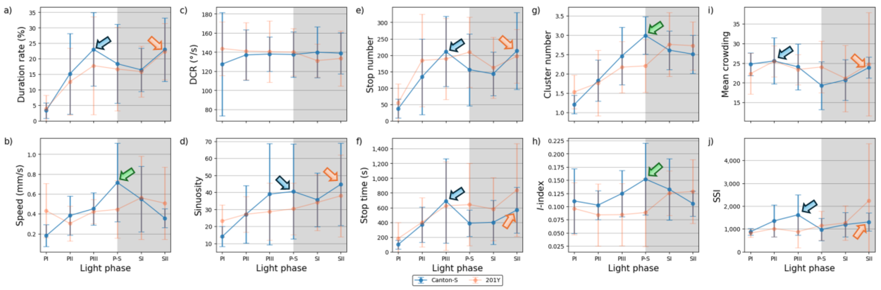
The duration rate varied between the micro-areas (Figure 5). In the food-provision and center-diffusion areas, the trend in the duration rate was similar across the light phases and between the two strains, with two peaks observed during the mid-photophase (13.1–14.7 % and 17.8–23.0 % for the food-provision and center-diffusion areas, respectively) (blue arrows, Figure 5a,b) and late scotophase (7.0–10.0 % and 22.3–23.0 %, respectively) (orange arrows, Figure 5a,b) for both strains. The duration rates in the center-diffusion area were higher (13.9 % during the photophase and 19.7 % during the scotophase on average) than in the food-provision area (8.3 % and 8.5 % on average, respectively).
The duration rate for the areas related to activity (Figure 5c,d) was substantially different from those areas that provided resources (Figure 5a,b). For Canton-S, the duration rate in the intermediate area was low during the early photophase (31.2 %), increased during P-S, and stayed at a similar level during the scotophase (42.8 %) (Figure 5c). In the edge area, the duration rate was substantially different from the other micro-areas, being initially very high at 63.2 % during PI, decreasing rapidly until PIII, and staying at a stable level around 26.9 % afterward for Canton-S (Figure 5d).
While the duration rate according to the light phase was similar between Canton-S and 201Y in the resource supply areas, changes due to strains were observed in the areas related to activity (Figure 5c,d). In the intermediate area, the duration rate for 201Y was higher during the photophase than for Canton-S, respectively with 47.5 % and 31.9 % on average, and lower during the scotophase, respectively with 37.9 % and 43.9 % on average (Figure 5c). Some differences in the duration rate were also observed in the edge area, being lower during the photophase (32.2 % on average) and higher during the scotophase (36.2 % on average) for 201Y than for Canton-S (45.9 % and 28.0 %, respectively) (Figure 5d).
As with the movement parameters, high variability in the SD was also observed for the duration rate. The SD range was higher for 201Y than for Canton-S, with a wide range during the photophase in the intermediate area and during PII–PIII in the food-provision and center-diffusion areas (Figure 5a–d). For Canton-S, the SD range was generally limited except during PII–PIII in the food-provision and center-diffusion areas.
Group behavior profiles are illustrated by the speed and duration rate in combination according to the light phase for the two strains in Figure 5e,f. For Canton-S, the speed reached its peak (1.0 mm/s) during P-S. Before P-S, a high duration rate in the food-provision area was observed during PIII (13.1 %) (blue arrow, Figure 5e), a consequence of the high speed during P-S after staying in the food-provision area during PIII. The speed continuously decreased after this until SII (0.6 mm/s) although the duration rate in the food-provision area increased again (9.6 %) for Canton-S (orange arrow, Figure 5e).
Different profiles for the speed and duration rates were observed for 201Y. During PIII, the duration rate in the center-diffusion area was high (17.8 %) (blue arrow, Figure 5f). However, unlike Canton-S, the speed continuously increased to reach its maximum (1.5 mm/s) during SII.
3.3. Dispersion Parameter Measurements
Spatial and temporal units were determined to obtain dispersion parameters. Clustering represents how many local groups are spatially observed in the cumulated group movement positions. In determining the spatial units, the threshold distance (ε) for clustering was examined from 2 mm to 8 mm at intervals of 2 mm across time window sizes from 10 s to 60 s at intervals of 10 s. The cluster numbers obtained using the different spatial units and time windows according to the light phase are listed in Figure A1 The number of clusters increased as the window size increased, while the trend in the cluster number according to the spatial unit size was similar overall, though there was a slight difference between the two strains during the late scotophase.
To examine the cluster patterns in more detail, we selected ε = 4 mm and 8 mm as the threshold distance, with 30 s as the window size. The trend over time for the cluster number with the two threshold distances was generally similar (Figure 6a,b). With ε = 8 mm, the cluster number (6.6–8.9 on average) was lower overall than ε = 4 mm (4.7–9.3). For Canton-S, the peak was delayed during SI (8.9) (green arrow, Figure 6b) and the cluster number decreased during PI–PIII (7.8, 7.1, and 6.6, respectively) for Canton-S, whereas the cluster number slowly increased with ε = 4 mm during this period (Figure 6a). Differences in the cluster number was observed for 201Y compared with Canton-S. For 201Y, the cluster number was low during PI and continuously increased until SII for both threshold distances (Figure 6a,b). In addition, the SD range was generally broad during the scotophase with ε = 4 mm and during the photophase with ε = 8 mm for 201Y.
The overall dispersion patterns for the movement positions were examined using the I-index. Because the I-index globally measures the dispersion pattern focusing on individual isolation over the entire observation arena, the determination of local spatial units was not necessary. Figure 7 presents the I-index for the cumulated movement positions across the entire observation arena for time windows of 10 s to 60 s under normalization. Generally, the values were narrow in a low range. The I-index was higher at a window size of 10 s (peaking at 0.19), decreasing dramatically as the time window increased from 20 s (peaking at 0.10)(Figure 7a).
The trend in the I-index values over time was generally consistent between the time windows (Figure 7b). The I-index peaked during P-S (0.04-0.19) for Canton-S, indicating that the isolation of the individuals was lowest during P-S. For 201Y, the I-index was low during the photophase (0.03–0.15) and increased afterward during the scotophase (0.03–0.18). The I-index according to the light phase followed a similar pattern to that for speed for both strains (Figure 4a). For Canton-S, the I-index and the speed both peaked during the same light phase (P-S). The trend in I-index values over time were also similar to the cluster number with ε = 4 mm (Figure 6a) for Canton-S. The pattern of change in the I-index for 201Y was similar to that for the speed in the overall observation arena (Figure 4a). The SD range for the I-index was broader overall for 201Y than for Canton-S and during the photophase than during the scotophase.
While the I-index describes the degree of individual isolation, mean crowding represents the local crowdedness within a particular spatial unit. Mean crowding was obtained according to time window sizes between 10 s and 60 s and spatial scales between 11.1 mm2 and 1,225.0 mm2 to determine the optimal unit size for space and time (Figure A2). Overall, the trend over time for the mean crowding was similar between the spatial size and time windows. However, the mean crowding values gradually increased with the time window size (Figure A2) in a manner similar to the cluster number (Figure A1).
The trends in the mean crowding values across the light phases with a spatial unit size of 25 mm2 and 100 mm2 and a window size of 30 s were selected for detailed comparison (Figure 6c,d). The overall trends over time were similar between the two spatial unit sizes and the two strains. These trends over time for the mean crowding were also similar to that for the duration rate overall in the food-provision and center-diffusion areas (Figure 5a,b), with two peaks observed during the photophase and scotophase (blue and orange arrows, respectively, Figure 6c,d).
A slight difference was observed between Canton-S and 201Y during PI with a spatial unit size of 100 mm2, being higher for 201Y than for Canton-S during this phase (Figure 6d). The SD range was also broader overall for 201Y than for Canton-S, especially during the photophase.
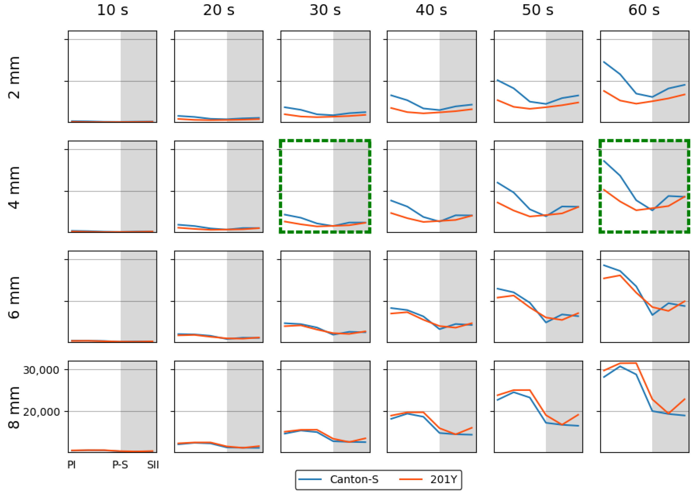
The SSI was also measured across different threshold distances and time window sizes as listed in Figure A3. While the SSI exhibited generally similar trends, the values increased as both the spatial distance and the time window size increased. With a threshold distance of 6 mm or lower, the SSI was higher for Canton-S and lower for 201Y. However, with a threshold distance of 8 mm, the SSI was lower for Canton-S and higher for 201Y (see the two green dotted rectangles shown as examples in Figure A3).
Although 4 mm is close to the critical distance for the SSI for Drosophila [2,39], we investigated the SSI with a threshold distance of 8 mm with the same time unit of 30 s for the purpose of comparison (Figure 6e,f). The shape of the trend in the SSI with a threshold distance of 4 mm was the opposite of that for the cluster number (Figure 6a) and similar to that for mean crowding (Figure 6c). Genetic differences in the SSI were found at the threshold distance of 4 mm; in particular, the SSI values were substantially lower for 201Y than for Canton-S, especially during the photophase (Figure 6e).
The trend in the SSI across the light phases at a threshold distance of 8 mm exhibited different patterns, with high values during PII ~ PIII (Figure 6f). The SSI values were remarkably similar between the two strains, with a maximum during PII (10,637.24) and a minimum (5,082.12) during SII for Canton-S, compared to a maximum during PIII (10,997.26) and a minimum during SI (5,116.39) for 201Y. SDs were overall higher for 201Y than for Canton-S, with SDs exceptionally high in photophase with the threshold distance of 8 mm for this strain.
3.4. Comparison of the Parameters Between Micro-Areas
Figure 8 presents overall view of the movement parameters with normalization for the micro-areas with a time window size of 30 s. The trends in the movement parameters over time were generally similar between the food-provision and center-diffusion areas, while these trends were variable in the intermediate and edge areas. In particular, the motility and sessility parameters were more variable between the light phases in the intermediate and edge areas (Figure 8). Sinuosity exhibited high variability in the edge area, while it was more stable with low values in the other micro-areas. The DCR was consistently observed within a limited range around an average of 140.9 °/s (though the change in direction, i.e., right or left, was not considered) across the light phases, indicating that large directional changes were observed during the 1 s time unit for group movement. Genetic differences in the motility parameters were also clearly observed in the intermediate and edge areas.
Figure 9 shows overview of the dispersion parameters with normalization for the micro-areas with a time window size of 30 s and with a threshold distance of 4 mm for the cluster number and SSI, a lattice size of 25 mm2 for the mean crowding, and the entire observation arena (19,600.0 mm2) for the I-index. Similar to movement parameters, the dispersion parameters were more variable in the intermediate and edge areas. The cluster number and the I-index were high in the intermediate area for Canton-S in accordance with the duration rate, while the cluster numbers were low in the food-provision and center-diffusion areas. The I-index was particularly high in the intermediate area, especially for 201Y, indicating a low degree of individual isolation. The cluster number and SSI were characterized by high values with a difference between the two strains at the edge of the area (Figure 9).
The movement and dispersion parameters are presented together for each micro-area in Figure 10, Figure 11, Figure 12 and Figure 13, focusing on trends over time. The trends for the parameters were similar overall between the resource supply areas (i.e., food and humidity), while those in areas related to activity (i.e., open space in the intermediate area and edge) varied greatly.
Coinciding trends were found for some measured parameters for Canton-S across the light phases depending on the micro-area. In the food-provision area, two major trends were observed over time. The first trend was a single peak for speed (0.6 mm/s) and the I-index (0.2) during P-S (green arrows, Figure 10b,h), while the second trend was two peaks during PII ~ PIII and SII for the duration rate (PIII: 13.1 %; SII: 9.6 %), stop number (PIII: 135.9; SII: 55.5), stop time (PII: 357.0 s; SII: 145.0 s), cluster number (PIII: 1.2; SII: 1.2), mean crowding (PII: 27.0; SII: 25.2), and SSI (PII: 1,645.5; SII: 1,367.5) (blue and orange arrows, Figure 10a,e–g,i,j). Most of the dispersion parameters except for the I-index exhibited two peaks in the food-provision area. The coinciding parameters with two peaks reflected local aggregations for feeding along with maximum durations in the food provision area.
Sinuosity exhibited a unique pattern with an early increase during the photophase to reach the highest level during PIII ~ P-S, followed by a slight decrease during the scotophase for Canton-S in the range of 13.0–24.7 (Figure 10d). The DCR was stable across the light phases at around 148.6 °/s (Figure 10c).
When comparing Canton-S and 201Y, the trends according to the light phase were substantially different for the speed and I-index, whereas similar patterns were observed over time for the other parameters. While Canton-S had a maximum speed during P-S (0.6 mm/s) and a clear diel difference, the diel difference for 201Y was less distinct, with low values during the photophase (0.4 mm/s) and a high value during the scotophase (0.6 mm/s) (Figure 10b). The I-index was low overall (0.10–0.12) until P-S, followed by an increase during SI ~ SII (0.14–0.15) for 201Y, which was in contrast to the single peak during P-S for Canton-S (Figure 10h). The stop number and stop time also differed, with higher averages during the photophase (135.9 and 357.0 s, respectively) and lower averages during SII (55.5 and 149.5 s, respectively) for 201Y than for Canton-S (Figure 10e,f).
SDs were variably expressed according to parameters, light phases and micro-areas (vertical bars, Figure 10-12). Since the parameter values were not normalized, the degree of variability cannot be comparable with other parameters objectively in these figures The quantitative degree of variability, expressed as coefficient of variation (CV; ratio of SD to mean) of measured parameters, will be discussed in ‘Section 4.5 Data variability and statistical differentiation’. In Figure 10-12, relative SD sizes across light phases are described in different parameters in two strains.
In the food-provision area for 201Y, distinctively high SDs were observed in photophase with duration rate, stop number and time, and SSI (Figure 10a,e,f,j) and in scotophase with speed (Figure 10b). The cluster number had intermittently high SDs in photo- and scoto-phases for 201Y (Figure 10g). Outstanding SDs were relatively fewer for Canton-S than for 201Y. SDs were high in scotophase with speed, mean crowding and I-index (Figure 10b,j,i), and were intermittently high in photophase with duration rate and sinuosity Canton-S (Figure 10a,d).
The parameter trends in the center-diffusion area (Figure 11) were generally similar to those for the food-provision area (Figure 10). Single peaks during P-S were observed for the speed (0.7 mm/s), cluster number (3.0), and I-index (0.15) for Canton-S (Figure 11b,g,h). A single peak was also observed for the cluster number during P-S in the center-diffusion area (Figure 11g), whereas the cluster number had double peaks in the food provision area (Figure 10g). Sinuosity also exhibited double peaks in the center-diffusion area during P-S (40.5) and SII (44.7) (Figure 11d), contrary to the trend of sinuosity in the food-provision area that showed the highest level during PIII ~ P-S for Canton-S (Figure 10d). Similar to the case of the food provision area the coinciding parameters with two peaks reflected local aggregations for obtaining humidity along with maximum durations in the center-diffusion area.
Figure 11.
Movement and dispersion parameters in the center-diffusion area across light phases for Canton-S and 201Y of D. melanogaster. (a) Duration rate, (b) speed, (c) DCR, (d) sinuosity, (e) stop number, (f) stop time, (g) cluster number, (h) I-index, (i) mean crowding and (j) SSI.
Figure 11.
Movement and dispersion parameters in the center-diffusion area across light phases for Canton-S and 201Y of D. melanogaster. (a) Duration rate, (b) speed, (c) DCR, (d) sinuosity, (e) stop number, (f) stop time, (g) cluster number, (h) I-index, (i) mean crowding and (j) SSI.
The sinuosity, cluster number, mean crowding, and SSI (Figure 11d,g,i,j) were considerably different for 201Y compared with Canton-S in the center-diffusion area, while the other parameters had similar trends between two strains to those observed for the food-provision area. The sinuosity exhibited two peaks over time for Canton-S and a linear increase toward the scotophase for 201Y (Figure 11d). Mean crowding and SSI also had two peaks for Canton-S, whereas these peaks were not observed for 201Y (Figure 11i,j). The cluster number had a single peak during P-S for Canton-S, which was in contrast to the linear increase observed for 201Y (Figure 11g). Although similar, minor differences were found in the stop number and stop time between the two strains, with higher stop numbers (PII ~ P-S: 167.2; SII: 213.2 on average) and stop times (P-S: 641.1 s; SII: 839.4 s on average) for 201Y (Figure 11e,f).
SDs in the center-diffusion area were observed with similarities and differences compared to the food-provision area. For 201Y, high SDs were observed in photophase with duration rate and stop number (Figure 11a,e) and in scotophase with speed, mean crowding and SSI (Figure 11b,i,j). The stop time was intermittently high in both photo- and scoto-phases (Figure 11f). In Canton-S, high SDs were observed in photophase with duration rate, DCR and stop time (Figure 11a,c,f) and in scotophase with speed (Figure 11b). The stop number was intermittently high in both photo- and scoto-phases in Canton-S (Figure 11e). It is noted that high SDs of duration rate and speed were observed in photophase and scotophase, respectively, in both strains in the food-provision and center-diffusion areas commonly (Figure 10a,b and Figure 11a,b). Extremely high SDs were observed with mean crowding and SSI during SII for 201Y compared with Canton-S (Figure 11i,j), whereas SD of DCR was outstandingly high during PI for Canton-S compared with 201Y (Figure 11c).
In the intermediate area, substantial differences were found in the parameter trends across the light phases (Figure 12) compared to the areas for resource provision. Increases were observed for the duration rate (21.5 % on average), speed (0.3 mm/s on average), stop number (81.9 on average), and stop time (199.2 s on average), compared with the center-diffusion area for Canton-S, while a decrease was observed for sinuosity (28.1 on average). The trend for speed in the intermediate area (green arrow, Figure 12b) was similar to that observed for the food-provision and center-diffusion areas, with a single peak during P-S for Canton-S. The two peaks observed for the number of parameters during the photophase and scotophase in the food-provision and center-diffusion areas were not observed in the intermediate area.
Figure 12.
Movement and dispersion parameters in the intermediate area across light phases for Canton-S and 201Y of D. melanogaster. (a) Duration rate, (b) speed, (c) DCR, (d) sinuosity, (e) stop number, (f) stop time, (g) cluster number, (h) I-index, (i) mean crowding and (j) SSI.
Figure 12.
Movement and dispersion parameters in the intermediate area across light phases for Canton-S and 201Y of D. melanogaster. (a) Duration rate, (b) speed, (c) DCR, (d) sinuosity, (e) stop number, (f) stop time, (g) cluster number, (h) I-index, (i) mean crowding and (j) SSI.
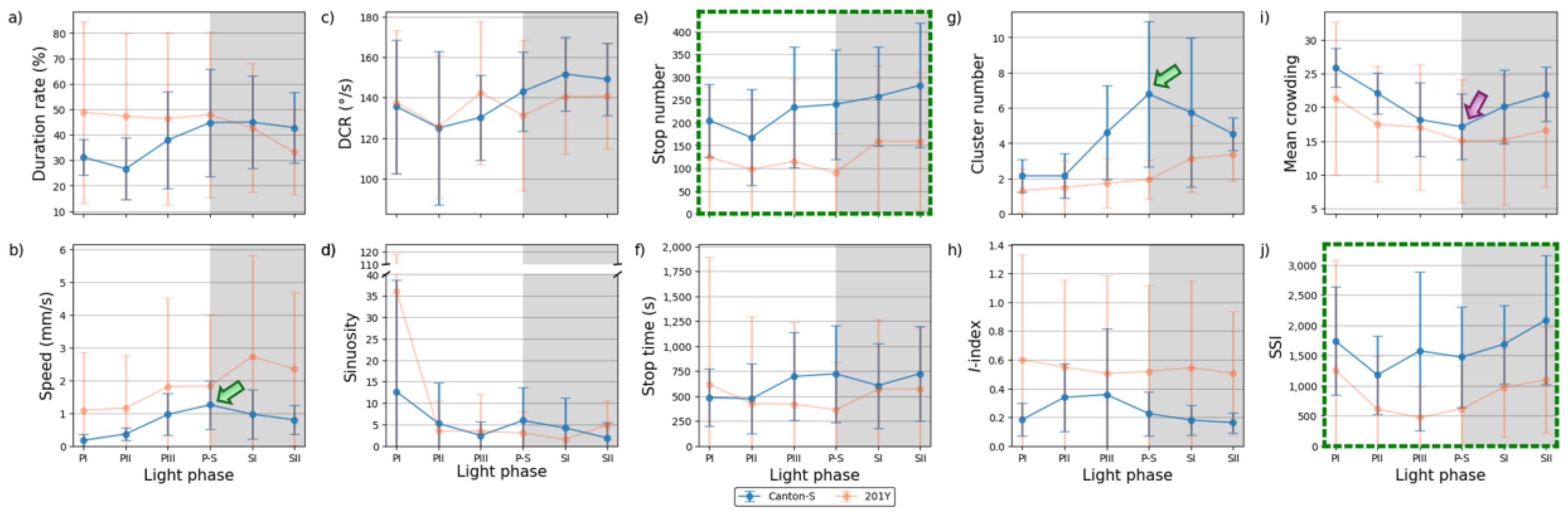
In the intermediate area, a number of parameters were low during the photophase and high during the scotophase, including the duration rate (photophase: 31.9 %; scotophase: 43.9 %), speed (0.5 mm/s and 0.9 mm/s, respectively), and stop number (202.0 and 269.9, respectively) for Canton-S (Figure 12a,b,e). Except for the high value during PI (12.7), sinuosity was generally stable (4.0 on average) afterward (Figure 12d). The DCR was slightly variable (139.1 on average) in the intermediate area (Figure 12c).
Dispersion parameter patterns were also substantially different from those of the food-provision and center diffusion areas (Figure 12g–j). The cluster number had a single peak during P-S (6.8), matching the peak for speed (Figure 12b,g). The trends for the I-index, mean crowding, and SSI were different overall from each other for Canton-S. For mean crowding, the minimum (17.1) was observed in the intermediate area (purple arrow, Figure 12i). The I-index had a peak early during PIII (Figure 12h). Coinciding trends were also observed between parameters; the trend in the SSI was very similar to that for the stop number (solid rectangles, Figure 12e,j).
Differences in the parameters between Canton-S and 201Y were observed in the intermediate area. The duration rate differed between light phases, being higher in the photophase (47.5 % on average) and lower in the scotophase (37.9 % on average) for 201Y than for Canton-S (Figure 12a). Although the trend in the speed was similar between the two strains in the center-diffusion area (Figure 11b), the speed for 201Y (1.8 mm/s) was substantially higher overall than for Canton-S (0.8 mm/s) (Figure 12b) in the intermediate area. This suggested the high speeds observed for 201Y overall originated from high speeds in the intermediate area, especially during the scotophase. In accordance with this, the stop number was consistently lower for 201Y (124.3) than for Canton-S (231.1) across the light phases (Figure 12e). The stop time, however, did not differ significantly between the two strains except for a minor increase during PIII (697.1 s) and P-S (723.4 s) for Canton-S compared with 201Y (419.4 s and 362.7 s, respectively) (Figure 12f).
For 201Y, comparing to the center-diffusion area, increases in parameter values in the intermediate area were observed for duration rate (44.4 %) and speed (1.8 mm/s) (Figure 12a,b), while decreases were observed for sinuosity (8.8), stop number (124.3), and stop time (494.3 s) on average (Figure 12d–f). Sinuosity was much higher during PI for 201Y (36.1) than for Canton-S (12.7), indirectly indicating a high degree of searching around activity for 201Y. The patterns for the stop number and SSI over time were remarkably similar for both 201Y and Canton-S (dotted green rectangles, Figure 12e,j), suggesting that the balance between attraction and repulsion with regard to neighboring individuals through frequent stops was preserved in both wild type and the mutant.
The SD patterns in the intermediate area were substantially different from those observed in the food-provision and center-diffusion areas. In Canton-S, SDs of many parameters were relatively stable including duration rate, speed, stop number and time and mean crowding (Figure 12a,b,e,f,i). SDs were intermittently high in photophase with DCR, sinuosity and I-index (Figure 12c,d,h), and high in scotophase with cluster number (Figure 12g). SD of SSI was sporadically high in both photo- and scoto-phases for the same strain (Figure 12j). For 201Y, SDs were overall high with duration rate, speed, stop time, I-index and mean crowding (Figure 12a,b,f,h,i), and low with cluster number (Figure 12g) compared to Canton-S. Within 201Y, SDs were high in photophase in variable periods with duration rate, DCR, stop time (Figure 12a,c,f), and intermittently high in both photo- and scoto-phases with speed (Figure 12a). It is noted that SDs were exceptionally high with sinuosity during PI for both strains (Figure 12d).
The parameters in the edge area were substantially different from those in the other micro-areas (Figure 13). Peaks often observed in the resource provision areas were not found in the edge area for Canton-S. The peak for the speed (1.0 mm/s) was observed slightly later during SI in the edge area (green arrow, Figure 13b), compared with the peak during P-S in the other areas.
Figure 13.
Movement and dispersion parameters in the edge area across light phases for Canton-S and 201Y of D. melanogaster. (a) Duration rate, (b) speed, (c) DCR, (d) sinuosity, (e) stop number, (f) stop time, (g) cluster number, (h) I-index, (i) mean crowding and (j) SSI.
Figure 13.
Movement and dispersion parameters in the edge area across light phases for Canton-S and 201Y of D. melanogaster. (a) Duration rate, (b) speed, (c) DCR, (d) sinuosity, (e) stop number, (f) stop time, (g) cluster number, (h) I-index, (i) mean crowding and (j) SSI.
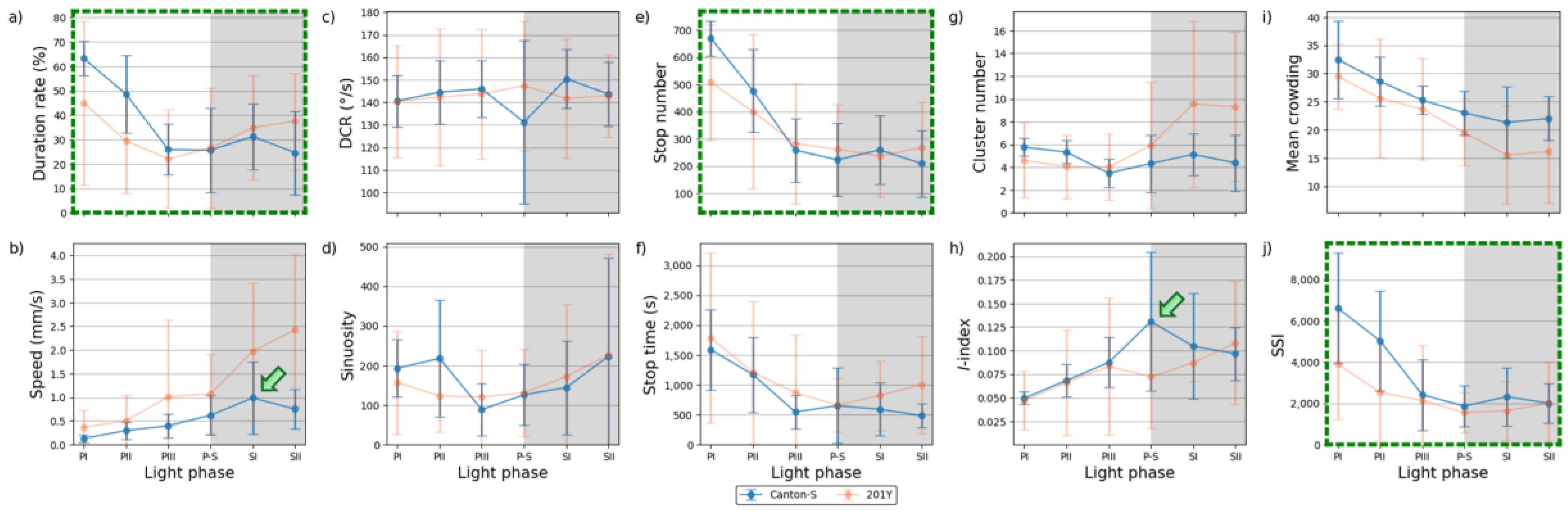
A substantial increase in the average sinuosity (165.2 on average) was observed in the edge area compared with the intermediate area (5.4 on average) for Canton-S (Figure 12d and 13d). A clear increase was also observed for the average SSI (3,371.9 on average) in the edge area (Figure 13j) compared with the intermediate (1,624.2 on average) and other areas, indicating a strong aggregation in the area close to boundary in the observation arena. Exceptionally high values were observed for the average duration rate (55.9 % on average), stop number (573.2 on average), and stop time (1,377.9 s on average) during PI ~ PII in the edge area (Figure 13a,e,f). The values later stabilized at an average of 26.9 % for the duration rate, 237.9 for the stop number, and 566.7 s for the stop time in the edge area. The DCR was stable with 142.9 °/s on average, although slight variation was observed during P-S.
The dispersion parameters in the edge area were also substantially different from those in the other micro-areas (Figure 13g-j). A peak during P-S was observed for the I-index (0.13) for Canton-S (green arrow, Figure 13h), matching the peak for speed (green arrow, Figure 13b). While the cluster number (4.7 on average) was stable across the light phases, high values were observed in early photophase for mean crowding (48.5) and the SSI (6,610.2) for Canton-S, but these decreased and stabilized during the scotophase (31.3 and 2,158.5, respectively, on average) (Figure 13i,j).
Differences in the behaviors of the two strains were also observed in the edge area. Of the movement parameters, the average duration rate was lower during the photophase (32.2 % on average) and higher during the scotophase (36.2 % on average) for 201Y compared with Canton-S (45.9 % and 28.0 % respectively, on average)(Figure 12a). The speed was also substantially higher across the light phases for 201Y than for Canton-S(Figure 12b). This difference was not great during the PI, but it continuously increased until SII, reaching 2.4 mm/s for 201Y compared to 0.8 mm/s for Canton-S (Figure 13b). Together with the faster speeds in the intermediate area, the speed in the edge area during the scotophase contributed greatly to the increase in the total speed of 201Y (Figure 4a). The trend in the stop number over time was similar between the two strains in the edge area (Figure 13e), whereas the stop number differed between the two strains especially in photophase in the intermediate area (Figure 12e). However, the DCR, sinuosity, stop number, and stop time were similar overall between the two strains (Figure 13c,e,f).
Coinciding patterns were also observed between parameters in the edge area. The patterns over time for the duration rate, stop number, and SSI were very similar between Canton-S and 201Y (green dotted rectangles, Figure 13a,e,j). The stop number and SSI were in accord in the intermediate area as stated above (green dotted rectangles, Figure 12e,j), while the duration rate was added to this group in the edge area, with very high values observed during the early photophase. This coinciding trend for the stop number and SSI in the areas related to activity persisted between strains.
The data variability pattern in the edge area was broadly similar to those in the intermediate area while allowing some local differences. The SDs for 201Y were high with duration rate, speed, DCR, stop time, cluster number, I-index and mean crowding compared with Canton-S (Figure 13a-c,f,g-i), similar to the case of the intermediate area. SDs increased correspondingly with the values of speed and cluster increasing as the time progressed toward scotophase for 201Y (Figure 13b,g). For Canton-S, SDs of many parameters were relatively stable including duration rate, speed, DCR, stop number and time, cluster number and mean crowding (Figure 13a-c,e-g,i), broadly similar to the intermediate area. SDs were intermittently high in photophase with SSI (Figure 13j) and high in scotophase with I-index (Figure 13h). SD of sinuosity was sporadically high in both photo- and scoto-phases in the same strain (Figure 13d).
In summary, common patterns were observed for the movement parameters across the light phases for Canton-S (Figure 10, Figure 11, Figure 12 and Figure 13):
- A peak during the early photophase followed by a minimum during the scotophase for the duration rate, stop number, and stop time in the edge area (Figure 13a,e,f);
- A peak during the early photophase along with a minimum during the scotophase for the duration rate, stop number, and stop time in the edge area (Figure 13a,e,f).
- Dispersion parameters also had frequently observed patterns across the light phases for Canton-S:
- A peak during the early photophase followed by a minimum during the scotophase for mean crowding and the SSI in the edge area (Figure 13i,j);
3.5. Data Variability and Statistical Differentiation
Because high variability was observed for the movement and dispersion parameters, the CV was used to compare the degree of variation in these parameters according to the micro-area, light phase, and strain. For the movement parameters, sinuosity overall exhibited high CVs for both strains (0.21–2.05 for Canton-S and 0.31–2.47 for 201Y) (Figure 14a). In contrast, CVs were low overall for the DCR for both strains (0.08–0.42 and 0.09–0.28, respectively).
CVs were high overall in the areas related to activity compared with the areas related to resource supply. In the food-provision area, the stop number (0.61–1.21), stop time (0.68–1.36) had higher ranges than the other parameters for Canton-S (Figure 14a). Stop number (0.46–0.85) and stop time (0.59–0.75) showed slightly high range of CVs than speed (0.27-0.61) and locomotory rate (0.28-0.79) in the center-diffusion area.
In the intermediate area, the I-index (0.43–1.29) had a high CV range followed by sinuosity (1.29–2.05), speed (0.55–0.99), locomotory rate (0.42–0.83), and SSI (0.38–0.83) for Canton-S (Figure 14a). In the edge area, the CV range was relatively low, being highest for sinuosity (0.38–1.11) and the locomotory rate (0.53–0.81).
The CVs for the movement parameters for 201Y were higher overall than those for Canton-S, while the CV trends within the micro-areas were similar (Figure 14a). Higher CVs were found in the intermediate area than in the other micro-areas, with many parameters exhibiting CVs over 1.0, including the sinuosity (1.14–2.47), stop time (1.07–2.07), speed (0.99–1.62), locomotory rate (0.86–1.61), stop number (0.95–1.58), SSI (0.80–1.45), and I-index (0.85–1.35) for 201Y (Figure 14). Differences between the two strains were also observed in the edge area. While the CVs for sinuosity were not much different as stated above, those for the speed (0.66–1.61), locomotory rate (0.61–1.53), and SSI (0.63–1.24) were higher for 201Y than for Canton-S (0.55–0.77, 0.53–0.81, and 0.63–1.24, respectively).
Figure 14b presents the CVs for the dispersion parameters according to the micro-area and light phase. The CVs for the dispersion parameters were generally lower than those for the movement parameters.
Among the micro-areas, the CVs were higher in the intermediate area for the SSI (0.17–0.83 for Canton-S and 0.22–1.45 for 201Y) and the I-index (0.13–1.29 and 0.22–1.35, respectively) compared with the other indices. The cluster number and mean crowding had low CVs in the food-provision (0.06–0.35 for Canton-S and 0.07–0.43 for 201Y) and center-diffusion areas (0.09–0.44 and 0.23–0.54, respectively) compared with the other micro-areas (Figure 14b).
Due to the high variability of parameters, statistically significant differences were observed in cases where the values of the parameters varied strongly. Figure 15 presents the statistical differentiation of the parameters between the micro-areas using Mann-Whitney U and Kolmogorov-Smirnov tests. For Canton-S, sinuosity was the most clearly differentiated movement parameters between the micro-areas during the light phases for both strains, whereas the DCR was not statistically different between these areas. Sessility (i.e., the stop number and stop time) and motility (i.e., the speed and locomotory rate) parameters exhibited some statistical differentiation between the micro-areas, light phases, and strains (Figure 15).
The movement parameters, stop number and stop time and the dispersion parameter cluster number were statistically differentiated in the intermediate and edge areas during PI ~ PII and in the food-provision area during PIII–SII for Canton-S (red dashed rectangle, Figure 15), indicating that the parameters for sessility and the cluster number were sensitive to differences in group behaviors between micro-areas. For the dispersion parameters, statistical differentiation was also observed for the I-index, mean crowding, and SSI, primarily in the edge area during PI (the last column of each heatmap plot for each parameter).
In contrast, the motility parameters were not as statistically distinct as the other parameters, except for differences observed in the speed and locomotory rate during PIII (in the intermediate area; third column of the heatmap plot) and SII (in the intermediate and edge areas; third and fourth columns of the heatmap plots). The locomotory rate had a slightly stronger differentiation than the speed (Figure 15).
The mutant 201Y exhibited similar statistical differentiation to Canton-S, but the degree of this differentiation was weaker for both movement and dispersion parameters (Figure 15), confirming the broader data variability of parameters observed for 201Y (e.g., Figure 10–13). Unlike with the I-index, the mean crowding and SSI during PII observed for Canton-S was not observed for 201Y (green solid rectangles, Figure 15). Differences in the speed and locomotory rate observed for Canton-S were not observed for 201Y (two blue dotted rectangles, Figure 15), indicating that differences in group behavior were weaker in the mutant.
Figure 16 presents the statistical differentiation between light phases for the movement and dispersion parameters in each micro-area in two strains. Differentiation of parameters according to the light phrase was consistently observed in the edge area (the vertical column matching the edge area for Canton-S, Figure 16), primarily during PI ~ PII (first and second columns within each heatmap plot). In the food-provision and center-diffusion areas, the motility and sessility parameters were statistically differentiated, while the cluster number in the dispersion parameters was differentiated in the center-diffusion area. The DCR was not statistically different except for a minor difference in the intermediate area. The I-index, mean crowding, and SSI were not differentiable between the micro-areas except in the edge area.
Statistical differentiation between light phases for 201Y was much weaker compared with Canton-S (Figure 16). No statistical differences were observed for 201Y except in the edge area and in the intermediate area. The statistical differences observed for the sinuosity, stop number, and stop time for Canton-S were not observed for 201Y, with only minor differences in the center-diffusion area for the stop number and stop time (green solid rectangle, Figure 16). Strong statistical differentiation was observed for the speed and locomotory rate for Canton-S, but this differentiation was not observed in most areas except the edge area for 201Y (red dashed rectangle, Figure 16). Similarly, the statistical differentiation observed for the I-index, mean crowding, and SSI for Canton-S was not observed for 201Y (blue dotted rectangles, Figure 16). These results indicated that the differences in the genetic make-up of 201Y more severely affected behaviors related to the light phases than the micro-areas.
Table 1 summarizes the statistical analysis of the movement and dispersion parameters for Canton-S and 201Y, with strong statistical differences highlighted in blue (p < 0.05) and green (p < 0.10) to show possibilities of separation between parameters with high variability in two strains.
Clear statistical differences were often observed in the parameters for sessility. In particular, the stop number was highly differentiated in the intermediate area, while the cluster number and SSI were highly differentiated in the intermediate area (Table 1). The locomotory rate was slightly more strongly statistically differentiable than the speed with higher significance during PI and SII. Overall, the statistical differentiation matched the differences in the parameters observed between the micro-areas (Figure 10–13).
4. Discussion and Conclusions
In the present study, the collective group behaviors of D. melanogaster in different micro-areas were characterized by movement and dispersion parameters for 10 individuals within an observation arena (14 cm × 14 cm). The parameters were systematically selected to investigate instantaneous movement (motility, sessility, and curvature) and dispersion (cluster number, I-index, mean crowding, and SSI). The results confirmed the natural tendency for local enhancement in D. melanogaster [1,2] at a relatively low density, over the entire observation period (24 h).
Interesting behavioral patterns were observed for Canton-S in the areas providing resources. In particular, a double-peak pattern consisting of a single peak during P-S (green arrows, Figure 4a,b, 10e,h and Figure 11e,g,h) and two peaks during the mid-photophase and the end of scotophase (blue and orange arrows, Figure 10a,e–g,i,j and Figure 11a,d-f,i,j) was recorded. A peak in the maximum duration rate was observed during PII–PIII in the food-provision and center-diffusion areas (blue arrows Figure 10a and 11a), followed by a single peak in the maximum speed during P-S (green arrows, Figure 10b and Figure 11b). It can be conjectured that the individuals stayed longer in the resource supply areas during PIII due to feeding. Subsequently, the speed increased to a maximum during P-S as a result of this energy intake (Figure 5e).
A peak during PII–PIII was also observed for the dispersion parameters mean crowding and SSI in the food-provision and center-diffusion areas (blue arrows, Figure 10i,j and 11i,j), and this was associated with the cluster number in the food-provision area (blue arrow, Figure 10g). This suggested that local aggregation was maximized during PII–PIII before reaching a maximum speed during P-S. In fact, peaks for mean crowding (Figure 10i and Figure 11i) and the SSI (Figure 10j) were observed even earlier during PII than the peak for the cluster number during PIII (Figure 10g and Figure 11g), indicating that local crowdedness and balancing between attraction and repulsion with neighboring individuals started before the maximum clustering for feeding during PIII. Individual isolation was also minimized based on evidence from the I-index during P-S (Figure 10h and Figure 11h) when speed was maximized in the food-provision and center-diffusion areas.
Coinciding trends were also observed in the areas of activity. In particular, the stop number and SSI were associated in the intermediate and edge areas across the light phases (rectangles, Figure 12e,j and Figure 13e,j). This indicated that the number of stops was concurrently associated with adjustments to the distance to maintain a balance between attraction and repulsion regarding neighboring individuals. These similarities for the SSI and stop number were also observed with the mutant strain 201Y (Figure 12e,j and Figure 13e,j), meaning that they were preserved even after genetic differentiation. Separately, the trend in the cluster number was similar to that for speed in the center-diffusion and intermediate areas for Canton-S and 201Y.
In the scotophase, coinciding patterns between parameters were also observed. In particular, a continuous decrease after P-S was observed for the speed and the I-index in most-areas except the intermediate area (Figure 10,11 and 13). In addition, a decrease during SI followed by an increase during SII was found for the duration rate, stop number, stop time, mean crowding, and SSI in the food-provision and center-diffusion areas (Figure 10 and 11), indicating local aggregations for obtaining resources along with maximum durations in the resource supply areas.
These results suggest that spatial group behavior was illustrated effectively by the movement and dispersion parameters. The coinciding patterns observed concurrently for the movement and dispersion parameters provide useful information on collective behavior mechanisms in response to external biological (e.g., neighbors) and environmental (e.g., food) factors. The underlying mechanisms responsible for spatial group formation in micro-areas as time progresses, however, are currently unknown. More research is required to investigate physiology–behavior relationships under a diverse range of experimental conditions.
Behavioral differences due to genetic differences were observed in the present study. Differences between wild-type strain Canton-S and mutant strain 201Y were recorded for various movement and dispersion parameters. A particularly notable difference was in the speed between the two strains (Figure 4a). While a peak was observed during P-S for Canton-S, the speed increased continuously after P-S for 201Y. This difference arises from the very high speeds observed for 201Y in the intermediate (Figure 12b) and edge (Figure 13b) areas, especially during the scotophase.
The mutant 201Y, as a mushroom body-specific GAL4 driver [59,60], has been used as a reference strain for investigating behavioral abnormalities after inducing the expression of genes under the control of upstream activating sequence (UAS). It was originally assumed that 201Y would not exhibit major behavioral changes, but it has been shown that the 201Y homozygous line affected courtship song [20], with the insertion of the GAL4 transgene within the first intron of TAK1-assosicated binding protein 2 (Tab2), which encodes a protein with an ubiquitin biding domain, potentially effecting the expression of Tab2. The reasons for the differences in the group behavior observed for 201Y in the present study are currently unknown, thus future neuro-physiological genetic research is required to understand these patterns.
Previous studies have investigated group behavior due to genetic differentiation using a variety of different methods. Schneider et al. [32] highlighted the benefits of integrating the history and pattern of interactions among individuals when identifying the molecular mechanisms that underlie the social modulation of behavior. Related research on physio-genetic mechanisms has also been reported, with the social space affected by parental age [61], genotype-by-social-environment interactions [12] and aggression due to social isolation [5]. In this respect, the present study provides a methodological foundation for investigating differences in behavior due to genetic composition based on the use of micro-areas.
Though behavioral differences were observed for groups in the present study, additional observations of the movement of individuals are required to determine whether it is qualitatively different from group behaviors or whether it varies between strains. However, given individual variability, a large number of trials would be required to observe individuals separately. Another future goal is to observe the same individual within groups by tracking every individual consistently over a long period of time.
Considerable variability in the parameters was observed between micro-areas and strains in the present study (e.g., Figure 14). However, even though the range of the SDs was high, the mean values for a number of the parameters were remarkably similar across micro-areas and between the two strains, such as the stop number and SSI in the intermediate and edge areas (Figure 12e,j and Figure 13e,j). These results contribute to making the parameter measurements reliable and support the understanding of collective behavior mechanisms by allowing for crosschecking between parameters.
The CVs varied broadly in accordance with the micro-area, light phase, and strain (Figure 14). While sinuosity exhibited the broadest range of CVs in the food-provision and center-diffusion areas, the sessility parameters had the broadest range in the food-provision area. The range of CVs was also broader for 201Y than for Canton-S. In contrast, the DCR had the narrowest range of CVs across the micro-areas and strains. This variability can be used to investigate the degree of plasticity in group behaviors. Indeed, behavioral variability related to genetic composition has been investigated for aggression [62], courtship [63], activity levels [64], grooming [65,66], and movement [67]. Genetic variation due to environment-constructing traits and social interactions have been reported to play a causal role in the plasticity of behavioral development in groups [16,68] in conjunction with physiological factors [13]. Our study constructed behavior profiles from the continuous observation of multiple parameters in different areas, and this would be an effective strategy for understanding plasticity in movement behaviors.
Although statistical power is generally low when comparing parameters with high variability, statistical differences were observed for the micro-areas, light phases, and genetic strains based on the combined results of Mann-Whitney U and Kolmogorov-Smirnov tests (Figure 15 and 16 and Table 1). Statistical differences were more strongly observed for Canton-S than for 201Y. The differences in sinuosity were consistently statistically significant between micro-areas across the light phases, whereas the DCR was not statistically different (Figure 15a). Among the micro-areas, statistically significant differences in group behavior were more clearly observed in the intermediate area and for sessility parameters. The information provided in this study is useful for differentiating group behaviors based on genetic factors.
In the present study, the duration rate in the edge area during PI was high compared to other micro-areas, being coincident with high stop number and time (Figure 13a). This may be because the starting location for the flies was the edge area. Although the flies were active after the acclimation period they may have stayed longer in the edge area during early photophase. More research is thus required to investigate group behavior in the edge area after using various forms of acclimation, including the use of anesthesia for medical purposes [69].
Automatic continuous monitoring of the group movements of D. melanogaster over 24 h using parameters based on instantaneous movement and dispersion of cumulated movement positions confirmed the natural tendency for local enhancement at a relatively low density. Coinciding patterns in the measured parameters were observed over time in the areas providing resources, with a peak in the duration rates along with maximum local aggregation early during the photophase (PII–PIII), followed by a peak in the maximum speed along with the cluster numbers during the transition from the photophase to the scotophase (P-S). Other coinciding patterns were found in the areas related to activity between the stop number and SSI across the light phases. The group spacing was effectively represented by the movement and dispersion parameters and provides in-depth information on the collective behavior mechanisms in response to biological and environmental factors. However, the specific factors responsible for spatial group formation in the micro-areas over time are currently unknown. More research is required to better understand physiology–genetics–behavior relationships under various experimental conditions.
Differences between the wild-type Canton-S and mutant 201Y strains were observed in various movement and dispersion parameters, with a notably higher speed for 201Y in the intermediate and the edge areas, especially during the scotophase. The current study thus provides a methodological foundation for monitoring group behavioral differences under various experimental conditions associated with different micro-areas.
Author Contributions
Conceptualization, Tae-Soo Chon; Methodology, Nam Jung and Yun Doo Chung; Software, Nam Jung and Chunlei Xia; Validation, Hye-Won Kim; Formal analysis, Nam Jung; Investigation, Hye-Won Kim; Resources, Yong-Hyeok Jang and Yun Doo Chung; Data curation, Yong-Hyeok Jang; Writing – original draft, Tae-Soo Chon; Writing – review & editing, Yun Doo Chung; Visualization, Chunlei Xia; Supervision, Tae-Soo Chon; Funding acquisition, Tae-Soo Chon.
Funding
This work was supported by a National Research Foundation of Korea (NRF) grant funded by the Korean government (MSIT) (RS-2022-NR069997).
Institutional Review Board Statement
Not applicable.
Informed Consent Statement
Not applicable.
Data Availability Statement
Software and data would be available from the authors upon request.
Conflicts of Interest
The authors declare no conflict of interest.
Abbreviations
The following abbreviations are used in this manuscript:
| 201Y | Tab2201Y(BDSC# 4440) |
| SSI | social space index |
| DCR | Direction change rate |
Appendix A
Figure A1.
Cluster numbers in cumulated movement positions according to DBSCAN across different levels of threshold distance (ε) and time window sizes with normalization for Canton-S and 201Y of D. melanogaster.
Figure A1.
Cluster numbers in cumulated movement positions according to DBSCAN across different levels of threshold distance (ε) and time window sizes with normalization for Canton-S and 201Y of D. melanogaster.
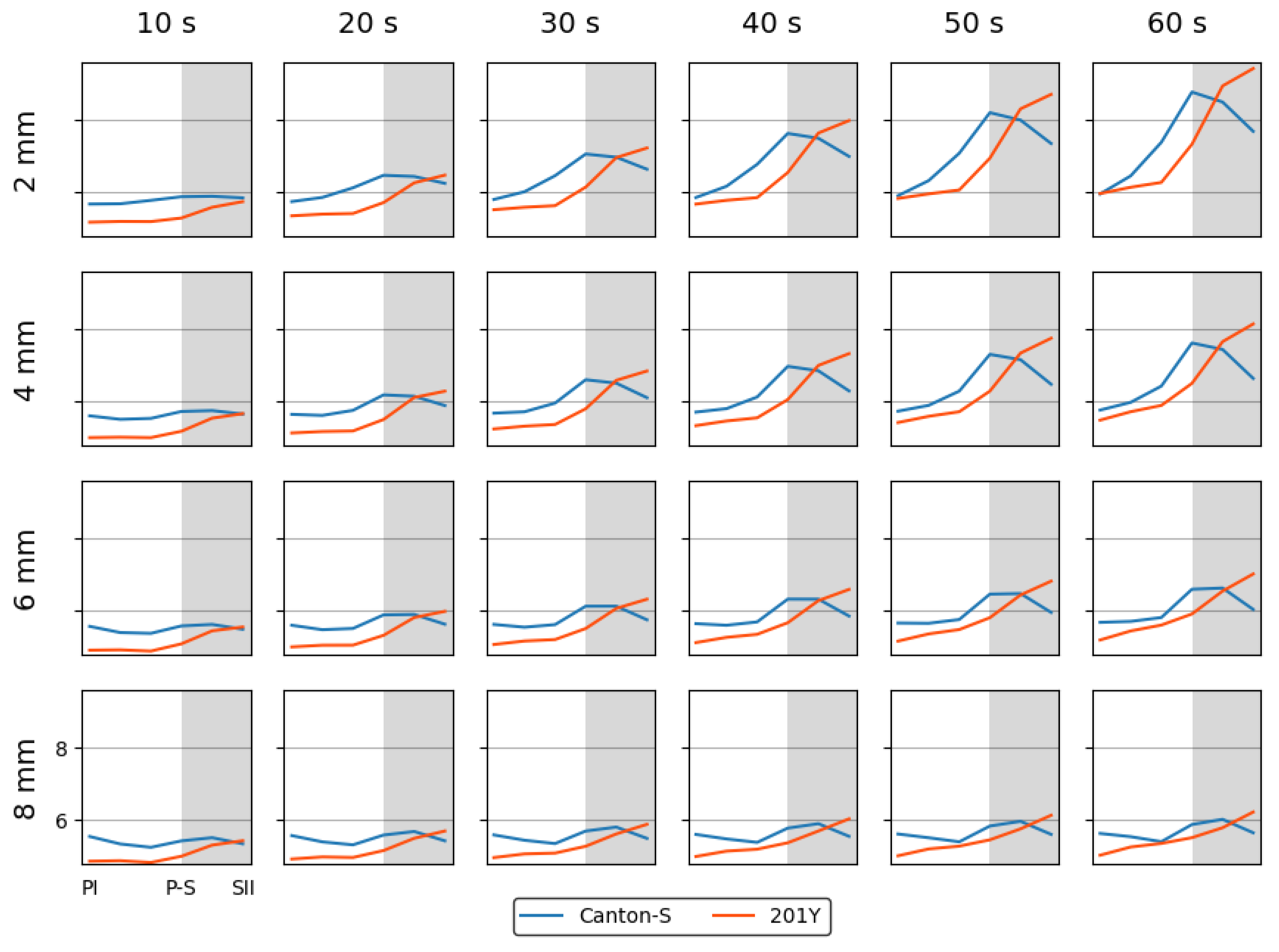
Figure A2.
Mean crowding of cumulated movement positions across different levels of lattice size and time window sizes with normalization for Canton-S and 201Y of D. melanogaster.
Figure A2.
Mean crowding of cumulated movement positions across different levels of lattice size and time window sizes with normalization for Canton-S and 201Y of D. melanogaster.
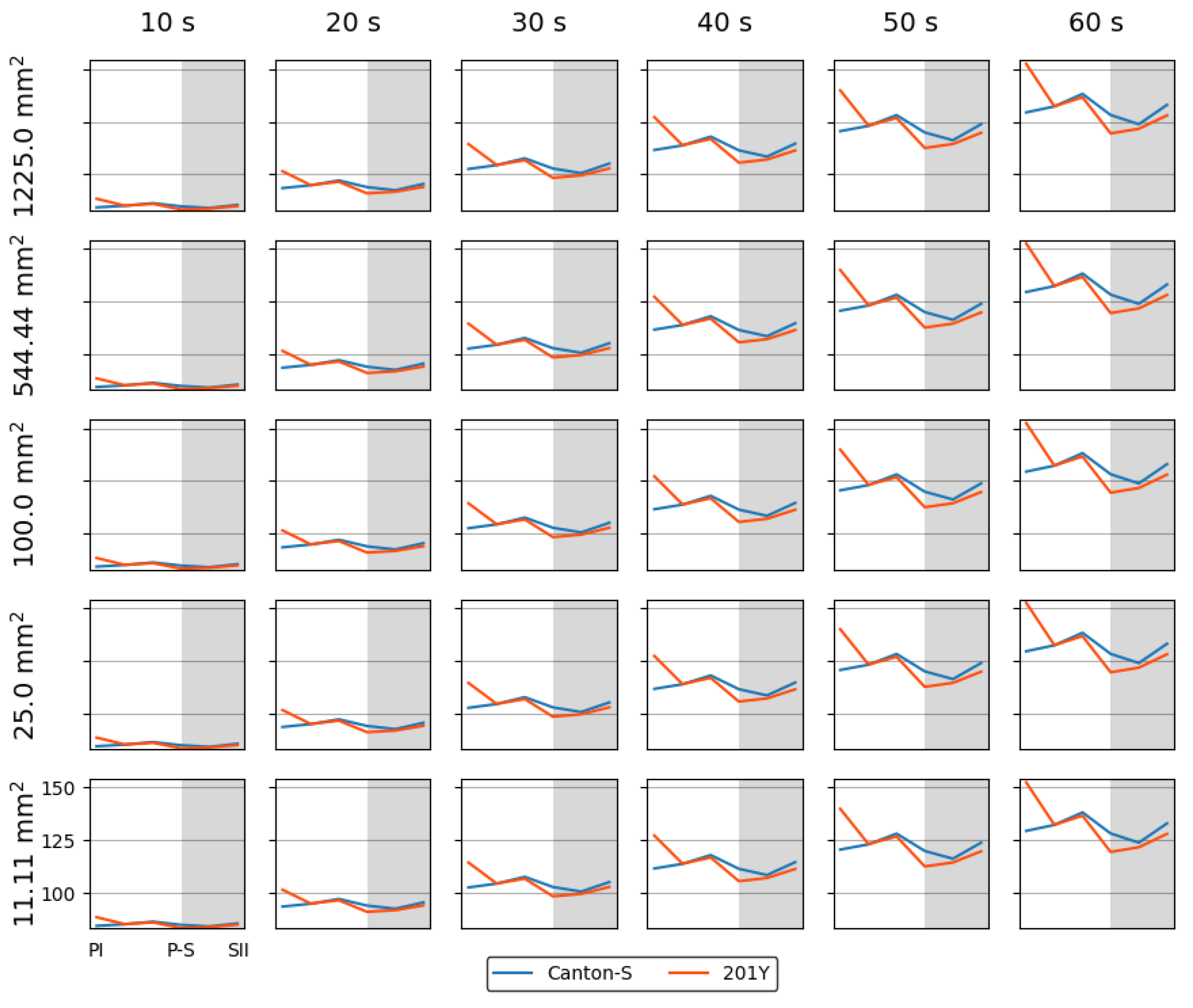
Figure A3.
SSI of cumulated movement positions across different levels of time window size with normalization for Canton-S and 201Y of D. melanogaster.
Figure A3.
SSI of cumulated movement positions across different levels of time window size with normalization for Canton-S and 201Y of D. melanogaster.
References
- Rohlfs, M.; Hoffmeister, T.S. Spatial aggregation across ephemeral resource patches in insect communities: an adaptive response to natural enemies? Oecologia 2004, 140, 654–661. [Google Scholar] [CrossRef] [PubMed]
- Simon, A.F.; Chou, M.T.; Salazar, E.D.; Nicholson, T.; Saini, N.; Metchev, S.; Krantz, D.E. A simple assay to study social behavior in Drosophila: measurement of social space within a group. Genes. Brain Behav. 2012, 11, 243–252. [Google Scholar] [CrossRef] [PubMed]
- Bartelt, R. J.; Schaner, A. M.; Jackson, L. L. cis-Vaccenyl acetate as an aggregation pheromone in Drosophila melanogaster. J. Chem. Ecol. 1985, 11, 1747–1756. [Google Scholar] [CrossRef]
- Liu, W.; Liang, X.; Gong, J.; Yang, Z.; Zhang, Y.H.; Zhang, J.X.; Rao, Y. Social regulation of aggression by pheromonal activation of Or65a olfactory neurons in Drosophila. Nat. Neurosci. 2011, 14, 896–902. [Google Scholar] [CrossRef]
- Agrawal, P.; Kao, D.; Chung, P.; Looger, L.L. The neuropeptide Drosulfakinin regulates social isolation-induced aggression in Drosophila. J. Exp. Biol. 2020, 223, 2. [Google Scholar]
- Ramdya, P.; Lichocki, P.; Cruchet, S.; Frisch, L.; Tse, W.; Floreano, D.; Benton, R. Mechanosensory interactions drive collective behaviour in Drosophila. Nature 2015, 519, 233–236. [Google Scholar] [CrossRef] [PubMed]
- Ferreira, C.H.; Moita, M.A. What can a non-eusocial insect tell us about the neural basis of group behaviour? Curr. Opin. Insect. Sci. 2019, 36, 118–124. [Google Scholar] [CrossRef]
- Chen, S.; Lee, A.Y.; Bowens, N.M. ; Huber,R.; Kravitz, E.A. Fighting fruit flies: a model system for the study of aggression. PANS. 2002. 99, 8, 5664-5668. [Google Scholar]
- Trannoy, S.; Penn, J.; Lucey, K.; Popovic, D.; Kravitz, E.A. Short and long-lasting behavioral consequences of agonistic encounters between male Drosophila melanogaster. PNAS 2016, 113, 4818–4823. [Google Scholar] [CrossRef]
- Chowdhury, B.; Wang, M.; Gnerer, J.P.; Dierick, H.A. The Divider Assay is a high-throughput pipeline for aggression analysis in Drosophila. Commun. Biol. 2021, 4, 1. [Google Scholar] [CrossRef]
- Penn, J.K.; Zito, M.F.; Kravitz, E.A. A single social defeat reduces aggression in a highly aggressive strain of Drosophila. PNAS 2010, 107, 12682–12686. [Google Scholar] [CrossRef]
- Rohde, P.D.; Gaertner, B.; Ward, K.; Sørensen, P.; Mackay, T.F. Genomic analysis of genotype-by-social environment interaction for Drosophila melanogaster aggressive behavior. Genetics 2017, 206, 1969–1984. [Google Scholar] [CrossRef] [PubMed]
- Chouhan, N.S.; Mohan, K.; Ghose, A. cAMP signaling mediates behavioral flexibility and consolidation of social status in Drosophila aggression. J. Exp. Biol. 2017, 220, 4502–4514. [Google Scholar]
- Edwards, A.C.; Rollmann, S.M.; Morgan, T.J.; Mackay, T.F.C. Quantitative genomics of aggressive behavior in Drosophila melanogaster. PLoS Genet. 2006, 2, e154. [Google Scholar] [CrossRef] [PubMed]
- Dierick, H.A.; Greenspan, R.J. Molecular analysis of flies selected for aggressive behavior. Nat. Genet. 2006, 38, 1023–1031. [Google Scholar] [CrossRef]
- Saltz, J. B. Genetic variation in social environment construction influences the development of aggressive behavior in Drosophila melanogaster. Heredity 2017, 118, 340–347. [Google Scholar] [CrossRef]
- Zhou, C.; Rao, Y.; Rao, Y. A subset of octopaminergic neurons are important for Drosophila aggression. Nat. Neurosci. 2008, 11, 1059–1067. [Google Scholar] [CrossRef]
- Alekseyenko, O.V.; Kravitz, E.A. Serotonin and the search for the anatomical substrate of aggression. Fly 2014, 8, 200–205. [Google Scholar] [CrossRef]
- Hoopfer, E.D. Neural control of aggression in Drosophila. Curr. Opin. Neurobiol. 2016, 38, 109–118. [Google Scholar] [CrossRef]
- Moran, C. N.; Kyriacou, C. P. Functional neurogenomics of the courtship song of male Drosophila melanogaster. Cortex 2009, 45, 18–34. [Google Scholar] [CrossRef]
- Wu, S.; Guo, C.; Zhao, H.; Sun, M.; Chen, J.; Han, C.; Peng, Q.; Qiao, H.; Peng, P.; Liu, Y.; Luo, S.D.; Pan, Y. Drosulfakinin signaling in fruitless circuitry antagonizes P1 neurons to regulate sexual arousal in Drosophila. Nat. Commun. 2019, 10, 4770. [Google Scholar] [CrossRef]
- Yamamoto, D.; Sato, K.; Koganezawa, M. Neuroethology of male courtship in Drosophila: from the gene to behavior. J. Comp. Physiol. A 2014, 200, 251–264. [Google Scholar] [CrossRef] [PubMed]
- Shao, L.; Chung, P.; Wong, A.; Siwanowicz, I.; Kent, C. F.; Long, X.; Heberlein, U. A neural circuit encoding the experience of copulation in female Drosophila. Neuron 2019, 102, 1025–1036. [Google Scholar] [CrossRef] [PubMed]
- Tinette, S.; Zhang, L.; Robichon, A. Cooperation between Drosophila flies in searching behavior. Genes. Brain Behav. 2004, 3, 39–50. [Google Scholar] [CrossRef]
- Kacsoh, B.Z.; Bozler, J.; Ramaswami, M.; Bosco, G. Social communication of predator-induced changes in Drosophila behavior and germ line physiology. Elife 2015, 4, e07423. [Google Scholar] [CrossRef] [PubMed]
- Lihoreau, M.; Clarke, I.M.; Buhl, C.; Sumpter, D.J.; Simpson, S.J. Collective selection of food patches in Drosophila. J. Exp. Biol. 2016, 219, 668–675. [Google Scholar] [CrossRef]
- Kretzschmar, D.; Tschäpe, J.; Bettencourt, D.C.A.; Asan, E.; Poeck, B.; Strauss, R.; Pflugfelder, G.O. Glial and neuronal expression of polyglutamine proteins induce behavioral changes and aggregate formation in Drosophila. Glia 2005, 49, 59–72. [Google Scholar] [CrossRef]
- Schneider, J.; Dickinson, M.H.; Levine, J.D. Social structures depend on innate determinants and chemosensory processing in Drosophila. Proc. Natl. Acad. Sci. USA 2012, 109 supplement_2, 17174–17179. [Google Scholar] [CrossRef]
- Sun, Y.; Qiu, R.; Li, X.; Cheng, Y.; Gao, S.; Kong, F.; Liu, L.; Zhu, Y. Social attraction in Drosophila is regulated by the mushroom body and serotonergic system. Nat. Commun. 2020, 11, 5350. [Google Scholar] [CrossRef]
- Dankert, H.; Wang, L.; Hoopfer, E.D.; Anderson, D.J.; Perona, P. Automated monitoring and analysis of social behavior in Drosophila. Nat. methods 2009, 6, 297–303. [Google Scholar] [CrossRef]
- Wang, L.; Han, X.; Mehren, J.; Hiroi, M.; Billeter, J.C.; Miyamoto, T.; Amrein, H.; Levine, J.D.; Anderson, D.J. Hierarchical chemosensory regulation of male-male social interactions in Drosophila. Nat. Neurosci. 2011, 14, 757–762. [Google Scholar] [CrossRef]
- Schneider, J.; Atallah, J.; Levine, J.D. Social structure and indirect genetic effects: genetics of social behaviour. Biol. Rev. 2017, 92, 1027–1038. [Google Scholar] [CrossRef]
- Palavicino-Maggio, C.B.; Trannoy, S.; Holton, K.M.; Song, X.; Li, K.; Nevo, E. Aggression and courtship differences found in Drosophila melanogaster from two different microclimates at Evolution Canyon, Israel. Sci. Rep. 2019, 9, 4084. [Google Scholar] [CrossRef] [PubMed]
- Burg, E.D.; Langan, S.T.; Nash, H.A. Drosophila social clustering is disrupted by anesthetics and in narrow abdomen ion channel mutants. Genes, Brain Behav 2013, 12(3), 338–347. [Google Scholar] [CrossRef] [PubMed]
- Ramdya, P.; Schneider, J.; Levine, J.D. The neurogenetics of group behavior in Drosophila melanogaster. J. Exp. Biol. 2017, 220, 35–41. [Google Scholar] [CrossRef] [PubMed]
- Jiang, L.; Cheng, Y.; Gao, S.; Zhong, Y.; Ma, C.; Wang, T.; Zhu, Y. Emergence of social cluster by collective pairwise encounters in Drosophila. Elife 2020, 9, e51921. [Google Scholar] [CrossRef]
- Simon, J.C.; Dickinson, M.H. A new chamber for studying the behavior of Drosophila. Plos one 2010, 5, e8793. [Google Scholar] [CrossRef]
- Jezovit, J.A.; Rooke, R.; Schneider, J.; Levine, J.D. Behavioral and environmental contributions to drosophilid social networks. PNAS 2020, 117, 11573–11583. [Google Scholar] [CrossRef]
- Sexton, O.J.; Stalker, H.D. Spacing patterns of female Drosophila paramelanica. Anim. Behav. 1961, 9, 77–81. [Google Scholar] [CrossRef]
- Navarro, J.; del Solar, E. Pattern of spatial distribution in Drosophila melanogaster. Behav. Genet. 1975, 5, 9–16. [Google Scholar] [CrossRef]
- Branson, K.; Robie, A.A.; Bender, J.; Perona, P.; Dickinson, M.H. High-throughput ethomics in large groups of Drosophila. Nat. Methods 2009, 6, 451–457. [Google Scholar] [CrossRef]
- Colomb, J.; Brembs, B. Sub-strains of Drosophila Canton-S differ markedly in their locomotor behavior. F1000Research 2015, 3, 176. [Google Scholar] [CrossRef] [PubMed]
- Strilbytska, O.; Strutynska, T.; Semaniuk, U.; Burdyliyk, N.; Bubalo, V.; Lushchak, O. Dietary sucrose determines stress resistance, oxidative damages, and antioxidant defense system in Drosophila. Scientifica 2022, 1, 7262342. [Google Scholar] [CrossRef] [PubMed]
- Edgecomb, R. S.; Harth, C. E.; Schneiderman, A. M. Regulation of feeding behavior in adult Drosophila melanogaster varies with feeding regime and nutritional state. J. Exp. Biol. 1994, 197, 215–235. [Google Scholar] [CrossRef]
- Nouhaud, P.; Mallard, F.; Poupardin, R.; Barghi, N.; Schlötterer, C. High-throughput fecundity measurements in Drosophila. Sci. Rep. 2018, 8, 4469. [Google Scholar] [CrossRef] [PubMed]
- What is YOLOv8_ A Complete Guide. Available online: https://blog.roboflow.com/what-is-yolov8/.
- Choi, K.H.; Kim, J.S.; Kim, Y.S.; Yoo, M.A.; Chon, T.S. Pattern detection of movement behaviors in genotype variation of Drosophila melanogaster by using self-organizing map. Ecol. Inform. 2006, 1, 219–228. [Google Scholar] [CrossRef]
- Liu, Y.; Chon, T.S.; Baek, H.; Do, Y.; Choi, J.H.; Chung, Y.D. Permutation entropy applied to movement behaviors of Drosophila melanogaster. Mod. Phys. Lett. B 2011, 25, 1133–1142. [Google Scholar] [CrossRef]
- Eom, H.J.; Liu, Y.; Kwak, G.S.; Heo, M.; Song, K. S.; Chung, Y. D.; Chon, T.S.; Choi, J. Inhalation toxicity of indoor air pollutants in Drosophila melanogaster using integrated transcriptomics and computational behavior analyses. Sci. Rep. 2017, 7, 46473. [Google Scholar] [CrossRef]
- Benhamou, S. How to reliably estimate the tortuosity of an animal's path:: straightness, sinuosity, or fractal dimension? J. Theor. Biol. 2004, 229, 209–220. [Google Scholar] [CrossRef]
- Campello, R. J.; Moulavi, D.; Sander, J. Density-based clustering based on hierarchical density estimates. In Adv. Knowl. Discov. Data. Min.; Springer: Berlin/Heidelberg, 2013; pp. 160–172. [Google Scholar]
- Johnson, R.B.; Zimmer, W.J. A more powerful test for dispersion using distance measurements. Ecology 1985, 66. 5, 1669–1675. [Google Scholar] [CrossRef]
- Lee, S.H.; Ji, C.W.; Chon, T.S. Change in spatial dispersion of Daphnia magna (Cladocera: Daphniidae) populations exposed to organophosphorus insecticide, diazinon. Environ. Anal. Health. Toxicol. 2009, 24, 231–240. [Google Scholar]
- Lloyd, M. 'Mean crowding' J. Anim. Ecol. 1967, 1–30. [Google Scholar] [CrossRef]
- Wade, M.J.; Fitzpatrick, C.L.; Lively, C.M. 50-year anniversary of Lloyd's “mean crowding”: Ideas on patchy distributions. J. Anim. Ecol. 2018, 87, 5, 1221–1226. [Google Scholar] [CrossRef]
- Mogilner, A.; Edelstein-Keshet, L. Spatio-angular order in populations of self-aligning objects: formation of oriented patches. Physica D 1996, 89, 346–367. [Google Scholar] [CrossRef]
- Sokal, R. R.; Rohlf, F. J. Biometry WH Freeman and Company. New York 1981, 4. [Google Scholar]
- Kwak, S. G.; Kim, J. H. Central limit theorem: the cornerstone of modern statistics. Korean J. Anesthesiol. 2017, 70, 144–156. [Google Scholar] [CrossRef] [PubMed]
- Yang, M.Y.; Armstrong, J.D.; Vilinsky, I.; Strausfeld, N.J.; Kaiser, K. Subdivision of the Drosophila mushroom bodies by enhancer-trap expression patterns. Neuron 1995, 15, 45–54. [Google Scholar] [CrossRef]
- O'Dell, K.M.; Armstrong, J.D.; Yang, M.Y.; Kaiser, K. Functional dissection of the Drosophila mushroom bodies by selective feminization of genetically defined subcompartments. Neuron 1995, 15, 55–62. [Google Scholar] [CrossRef]
- Brenman-Suttner, D.B.; Long, S.Q.; Kamesan, V.; de Belle, J.N.; Yost, R.T.; Kanippayoor, R.L.; Simon, A.F. Progeny of old parents have increased social space in Drosophila melanogaster. Sci. Rep. 2018, 8, 3673. [Google Scholar] [CrossRef]
- Mackay, T.F. Mutations and quantitative genetic variation: lessons from Drosophila. Philos. Trans. R. Soc. B Biol. Sci. 2010, 365, 1229–1239. [Google Scholar] [CrossRef]
- Griffith, L.C.; Ejima, A. Courtship learning in Drosophila melanogaster: diverse plasticity of a reproductive behavior. Learn. Mem. 2009, 16, 743–750. [Google Scholar] [CrossRef]
- Watanabe, L. P.; Gordon, C.; Momeni, M. Y.; Riddle, N. C. Genetic networks underlying natural variation in basal and induced activity levels in Drosophila melanogaster. G3: Genes, Genomes, Genetics 2020, 10, 1247–1260. [Google Scholar] [CrossRef] [PubMed]
- Mast, J.D.; De Moraes, C.M.; Alborn, H.T.; Lavis, L.D.; Stern, D.L. Evolved differences in larval social behavior mediated by novel pheromones. Elife 2014, 3, e04205. [Google Scholar] [CrossRef] [PubMed]
- Mueller, J.M.; Zhang, N.; Carlson, J.M.; Simpson, J.H. Variation and variability in Drosophila grooming behavior. Front. Behav. Neurosci. 2022, 15, 769372. [Google Scholar] [CrossRef]
- Thane, M.; Paisios, E.; Stöter, T.; Krüger, A.R.; Gläß, S.; Dahse, A.K.; Scholz, N.; Gerber, B.; Lehmann, D.J.; Schleyer, M. High-resolution analysis of individual Drosophila melanogaster larvae uncovers individual variability in locomotion and its neurogenetic modulation. Open Biology 2023, 13, 220308. [Google Scholar] [CrossRef] [PubMed]
- Makino, T.; Kawata, M. Habitat variability correlates with duplicate content of Drosophila genomes. Mol. Biol. Evol. 2012, 29, 3169–3179. [Google Scholar] [CrossRef]
- MacMillan, H. A.; Nørgård, M.; MacLean, H. J.; Overgaard, J.; Williams, C. J. A critical test of Drosophila anaesthetics: Isoflurane and sevoflurane are benign alternatives to cold and CO2. J. Insect. Physiol. 2017, 101, 97–106. [Google Scholar] [CrossRef]
Figure 1.
Observation system for detecting movement of Drosophila melanogaster (unit; mm). (a) Observation setup for continuous group movement, (b) closeup of observation frame (side view) and (c) observation arena (top view).
Figure 1.
Observation system for detecting movement of Drosophila melanogaster (unit; mm). (a) Observation setup for continuous group movement, (b) closeup of observation frame (side view) and (c) observation arena (top view).
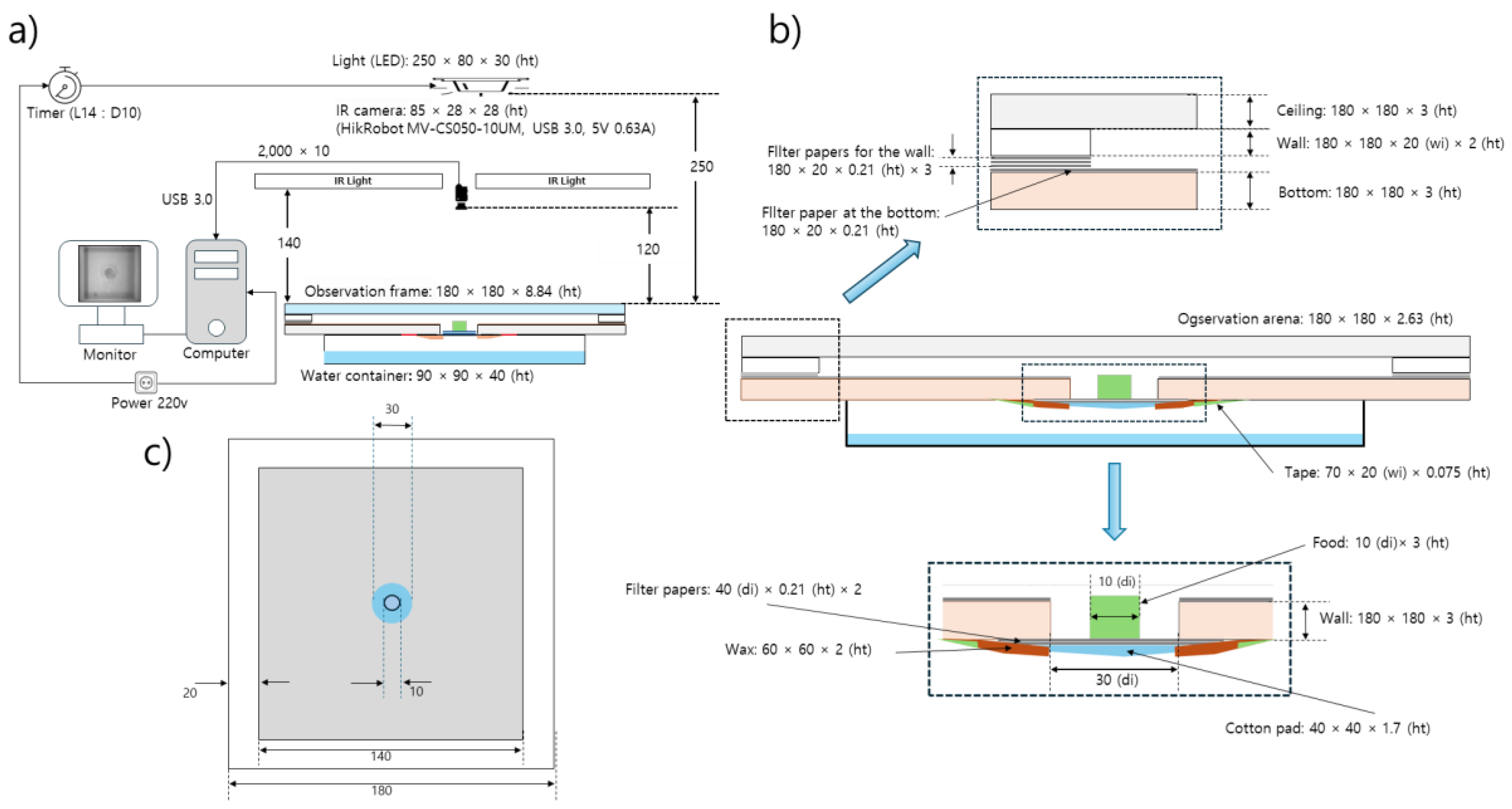
Figure 2.
Cumulated movement positions of M. drosophila and micro-areas within the observation arena. (a) Spatial positions for Canton-S, (b) for 201Y, and (c) micro-areas according to spatial clustering.
Figure 2.
Cumulated movement positions of M. drosophila and micro-areas within the observation arena. (a) Spatial positions for Canton-S, (b) for 201Y, and (c) micro-areas according to spatial clustering.
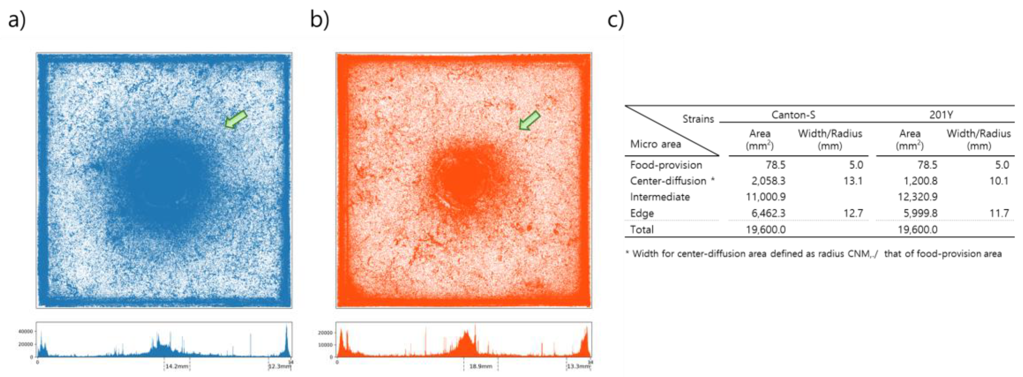
Figure 3.
Speed and DCR for group movement for Canton-S and 201Y of D. melanogaster in two strains. (a) Log-log graph for speed frequencies (blue; Canton-S and orange; 201Y), (b) histogram for short range speed, (c) histogram comparing speed in photo- and scoto-phases for Canton-S and (d) for 201Y, and (e) histogram comparing DCR in photo- and scoto-phases for Canton-S and (f) for 201Y.
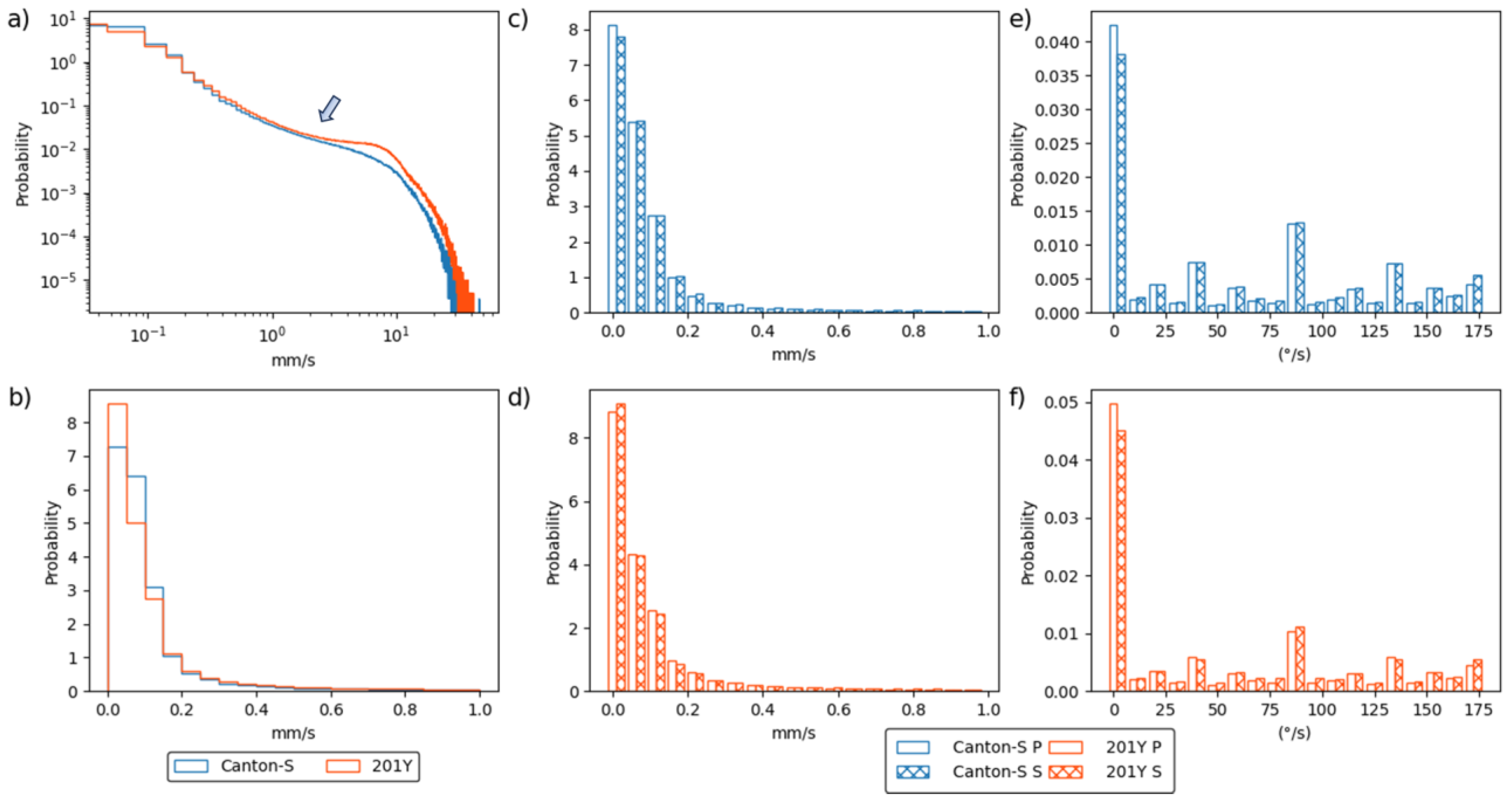
Figure 4.
Movement parameters in the observation arena across light phases for Canton-S and 201Y of M. drosophila. (a) Speed, (b) locomotory rate, (c) DCR, (d) sinuosity, (e) stop number and (f) stop time.
Figure 4.
Movement parameters in the observation arena across light phases for Canton-S and 201Y of M. drosophila. (a) Speed, (b) locomotory rate, (c) DCR, (d) sinuosity, (e) stop number and (f) stop time.
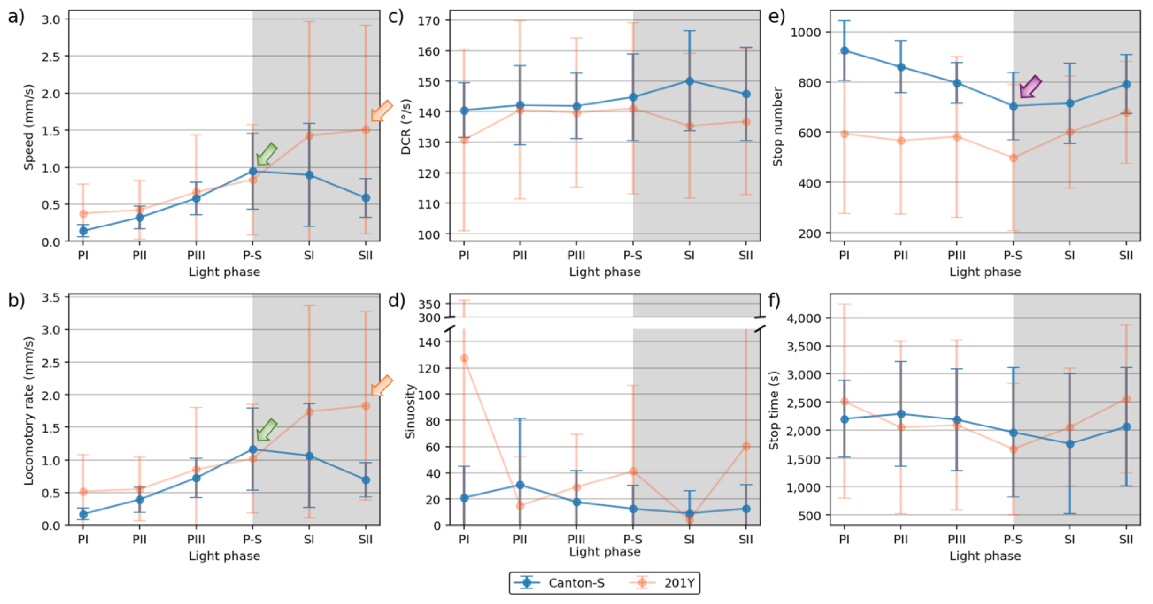
Figure 5.
Duration percentages at micro-areas and behavior profiles for Canton-S and 201Y of M. drosophila. (a) Durations (%) staying in the food provision, (b) center-diffusion, (c) intermediate and (d) edge areas within the observation arena, and (e) durations (%) superimposed with speed for Canton-S and (f) for 201Y.
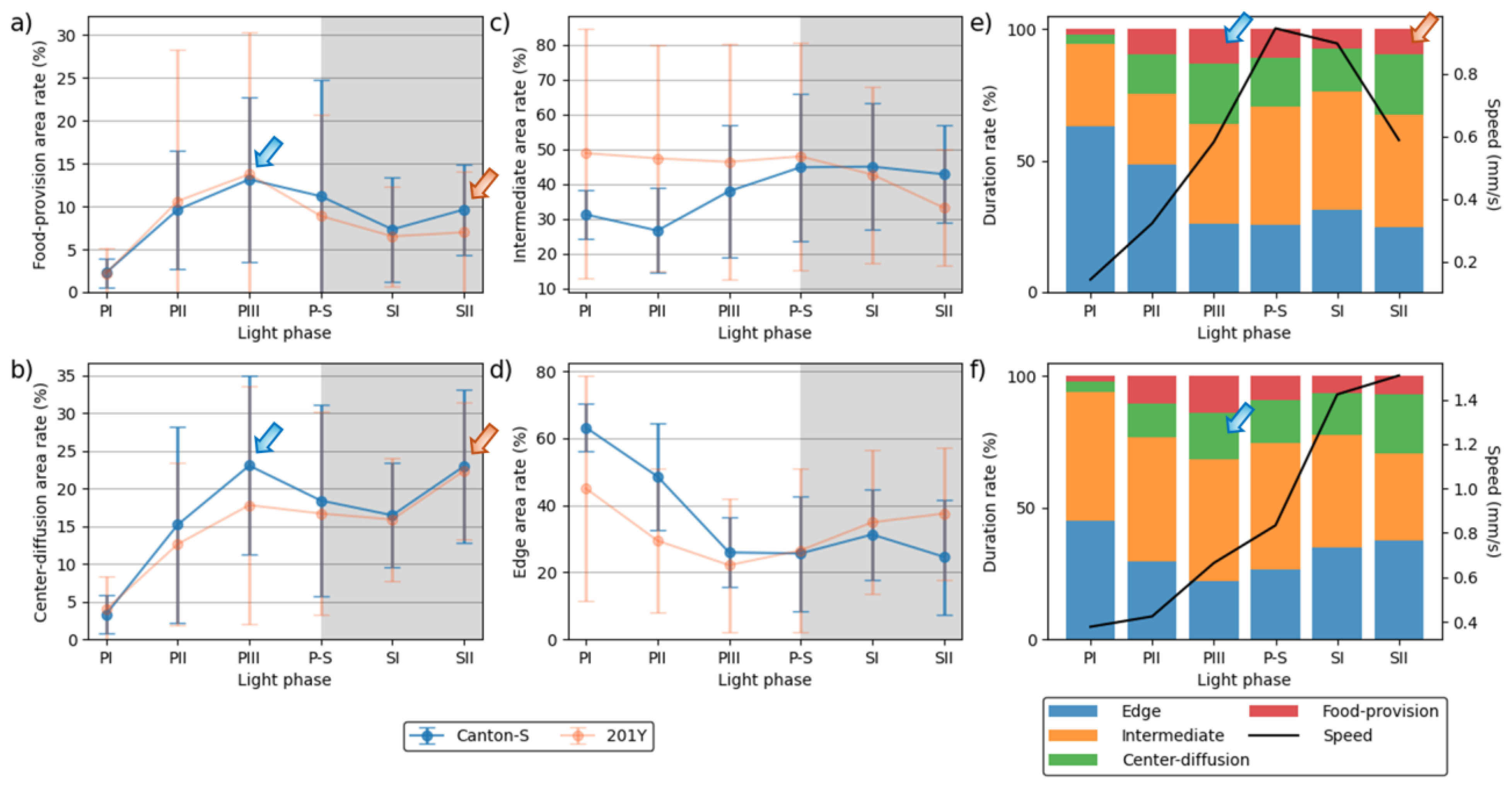
Figure 6.
dispersion parameters of group movement positions for Canton-S and 201Y of M. drosophila. (a) Cluster numbers with ε equal to 4 mm and (b) 8 mm, (c) mean crowding with unit size equal to 25 mm2 and (d) 100 mm2, and (e) SSI with threshold distance (l) equal to 4 mm and (f) 8 mm.
Figure 6.
dispersion parameters of group movement positions for Canton-S and 201Y of M. drosophila. (a) Cluster numbers with ε equal to 4 mm and (b) 8 mm, (c) mean crowding with unit size equal to 25 mm2 and (d) 100 mm2, and (e) SSI with threshold distance (l) equal to 4 mm and (f) 8 mm.
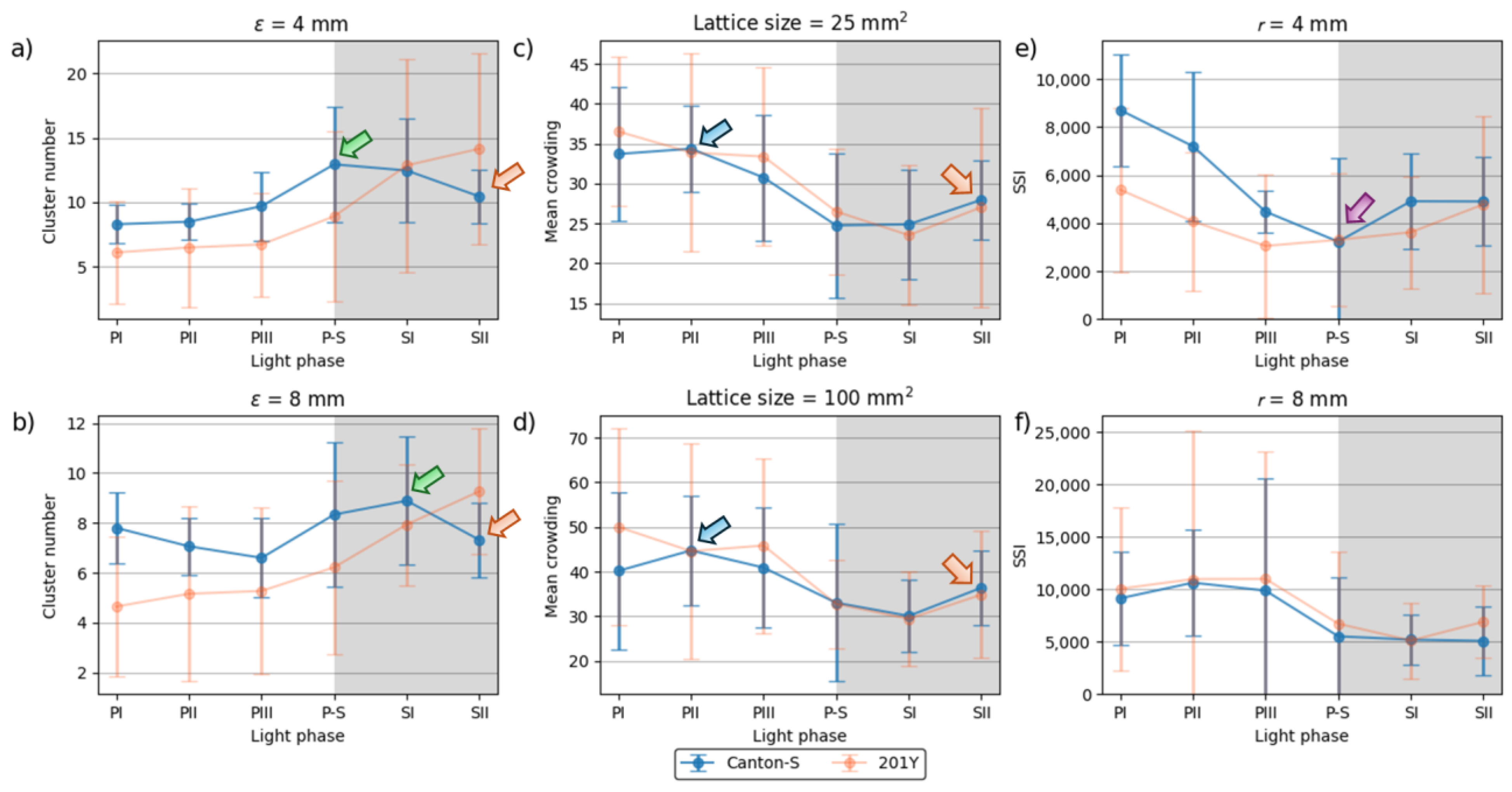
Figure 7.
I-index of cumulated movement positions in different time window sizes for Canton-S and 201Y of D. melanogaster. (a) Normalized values across time window sizes and (b) closeup of the curves.
Figure 7.
I-index of cumulated movement positions in different time window sizes for Canton-S and 201Y of D. melanogaster. (a) Normalized values across time window sizes and (b) closeup of the curves.
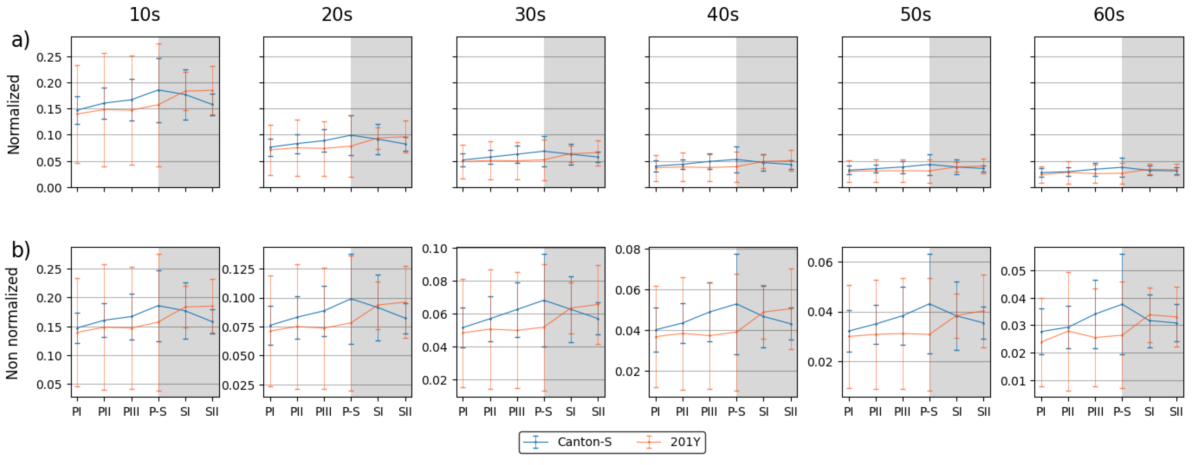
Figure 8.
Movement parameters in different micro-areas in the observation arena across light phases for Canton-S and 201Y of D. melanogaster (normalized across micro-areas).
Figure 8.
Movement parameters in different micro-areas in the observation arena across light phases for Canton-S and 201Y of D. melanogaster (normalized across micro-areas).
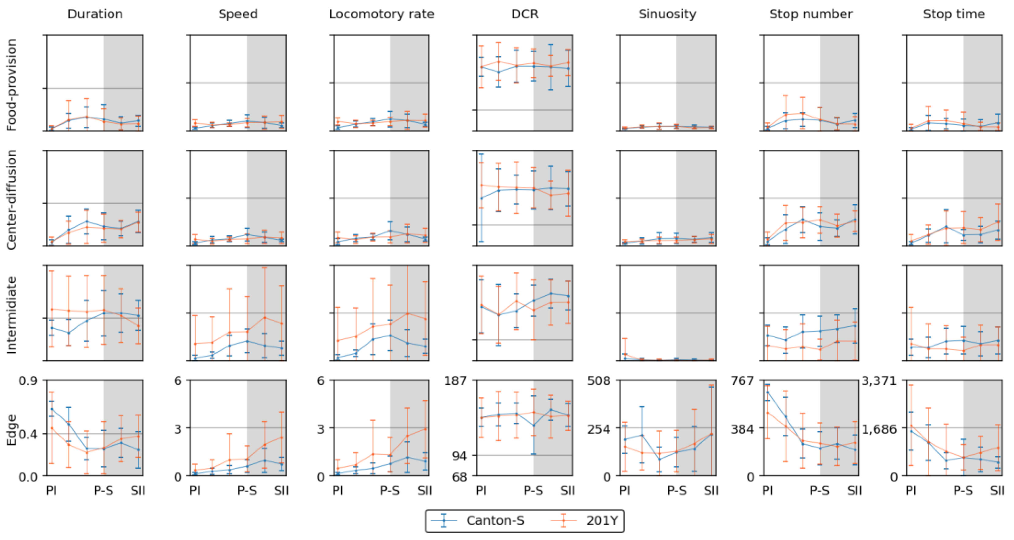
Figure 9.
Dispersion parameters in different micro-areas in the observation arena across light phases for Canton-S and 201Y of D. melanogaster (normalized across micro-areas).
Figure 9.
Dispersion parameters in different micro-areas in the observation arena across light phases for Canton-S and 201Y of D. melanogaster (normalized across micro-areas).
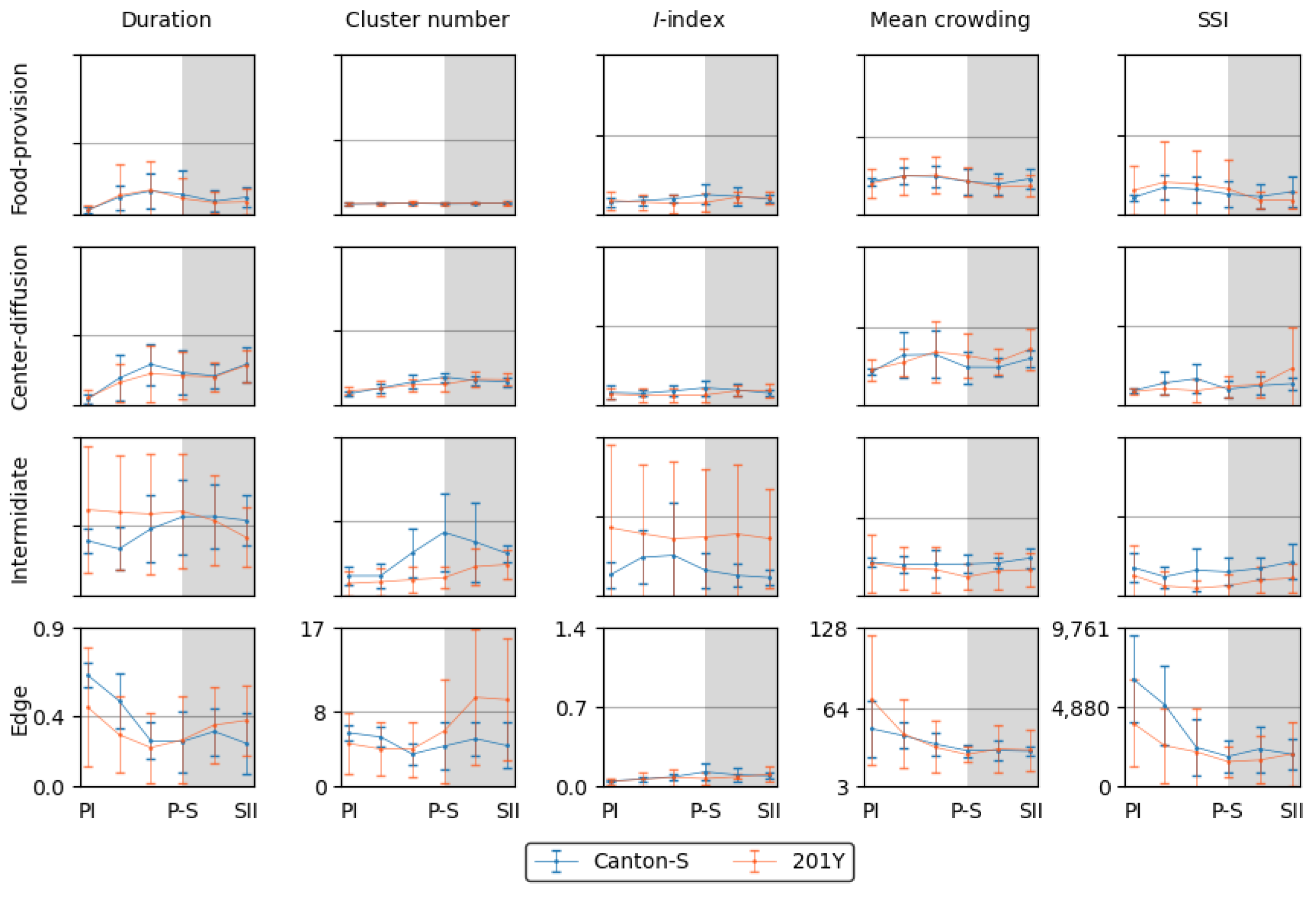
Figure 10.
Movement and dispersion parameters in the food-provision area across light phases for Canton-S and 201Y of D. melanogaster. (a) Duration rate, (b) speed, (c) DCR, (d) sinuosity, (e) stop number, (f) stop time, (g) cluster number, (h) I-index, (i) mean crowding and (j) SSI.
Figure 10.
Movement and dispersion parameters in the food-provision area across light phases for Canton-S and 201Y of D. melanogaster. (a) Duration rate, (b) speed, (c) DCR, (d) sinuosity, (e) stop number, (f) stop time, (g) cluster number, (h) I-index, (i) mean crowding and (j) SSI.
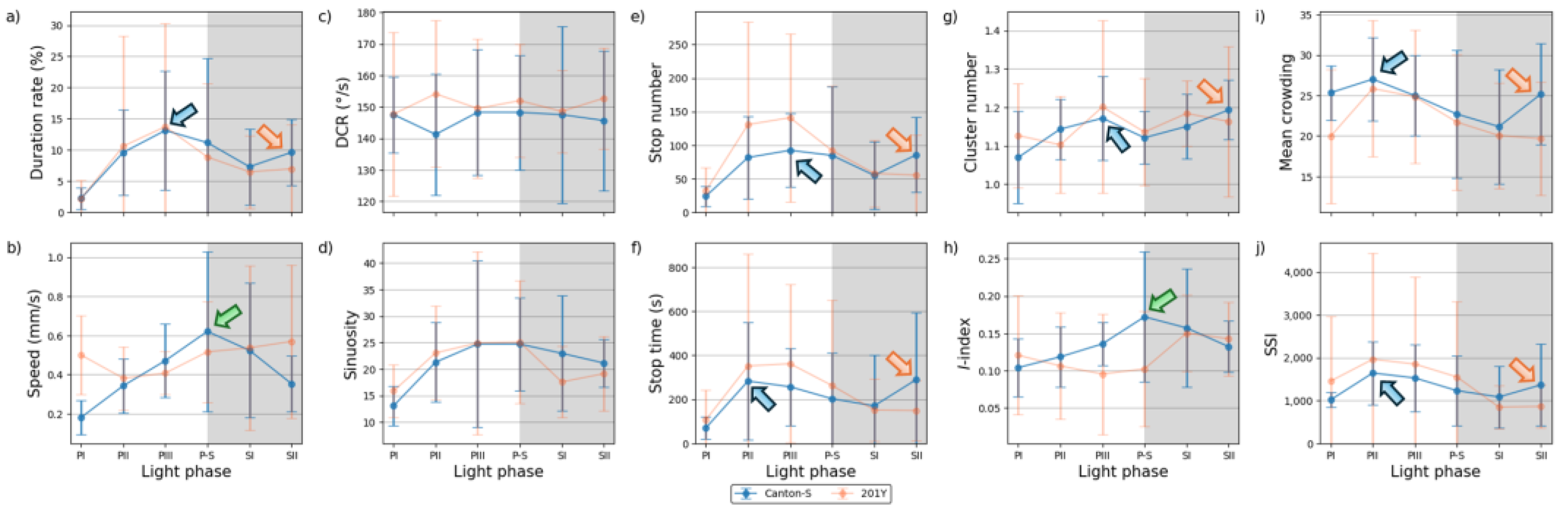
Figure 14.
Coefficient of variation for group movement parameters in each micro-area across light phases for Canton-S and 201Y of D. melanogaster. (a) Movement and (b) dispersion parameters.
Figure 14.
Coefficient of variation for group movement parameters in each micro-area across light phases for Canton-S and 201Y of D. melanogaster. (a) Movement and (b) dispersion parameters.
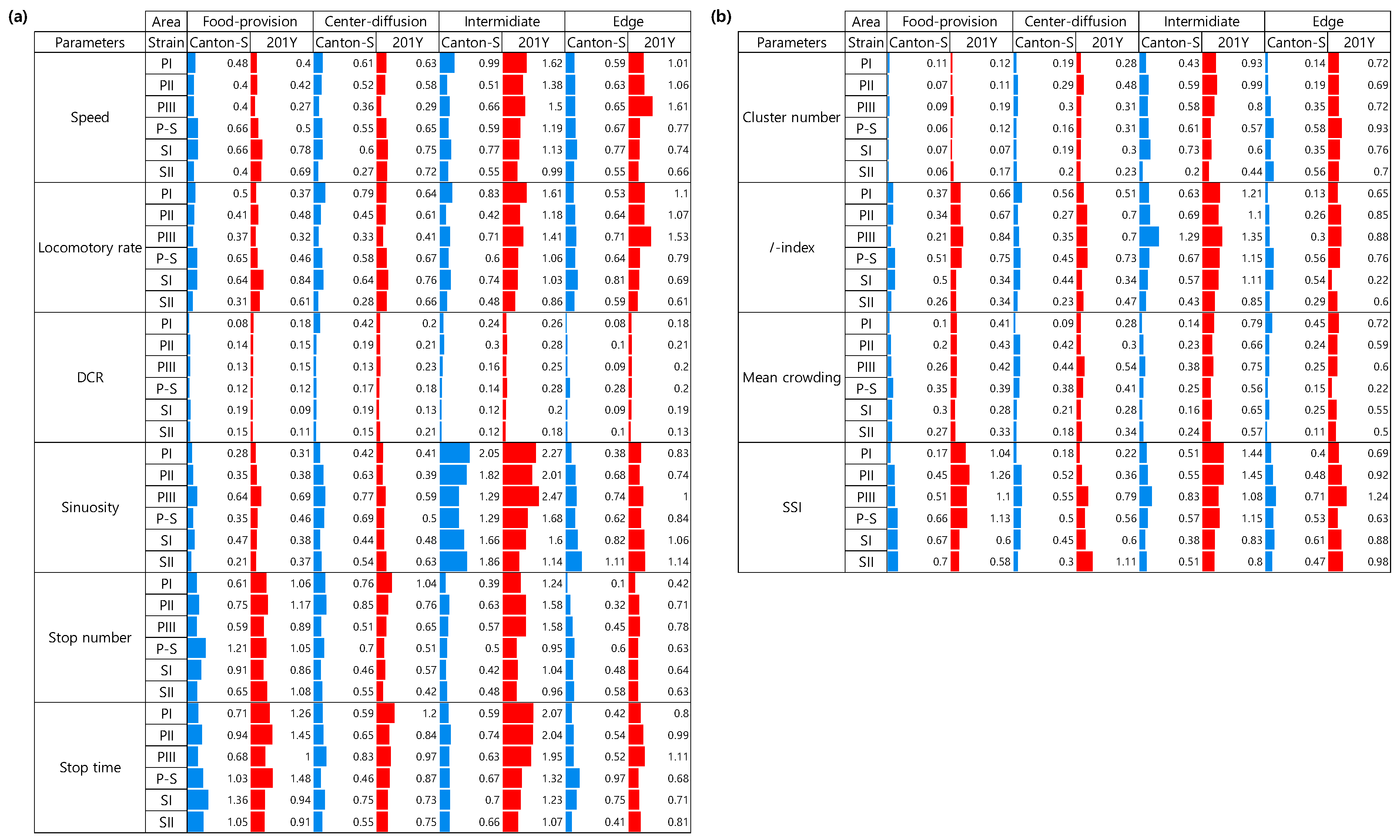
Figure 15.
Statistical differentiation of movement and dispersion parameters across micro-areas for Canton-S and 201Y of D. melanogaster according to results from Mann-Whitney U and Kolmogorov-Smirnov tests.
Figure 15.
Statistical differentiation of movement and dispersion parameters across micro-areas for Canton-S and 201Y of D. melanogaster according to results from Mann-Whitney U and Kolmogorov-Smirnov tests.
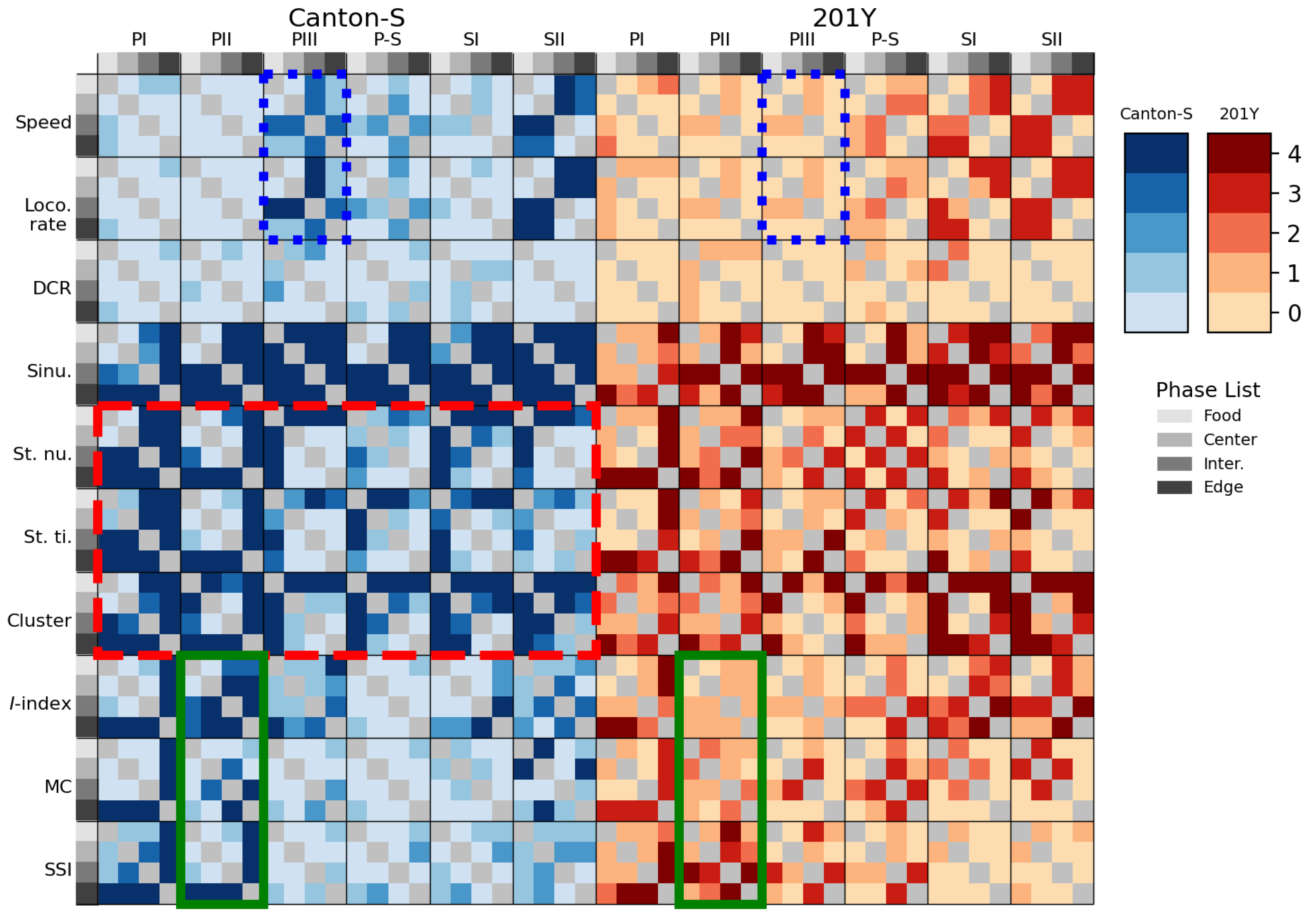
Figure 16.
Statistical differentiation of movement and dispersion parameters across light phases for Canton-S and 201Y of D. melanogaster according to results from Mann-Whitney U and Kolmogorov-Smirnov tests.
Figure 16.
Statistical differentiation of movement and dispersion parameters across light phases for Canton-S and 201Y of D. melanogaster according to results from Mann-Whitney U and Kolmogorov-Smirnov tests.
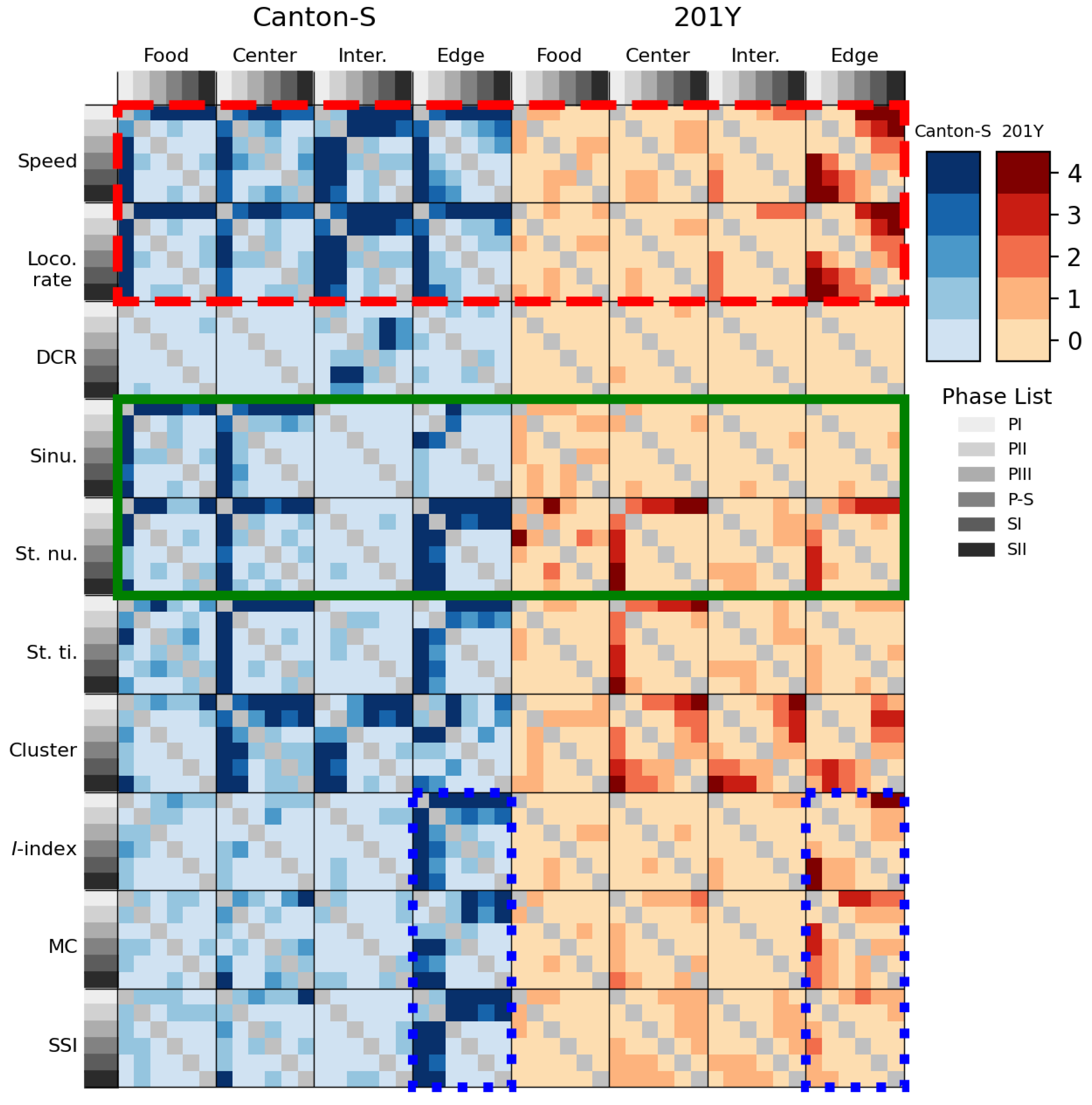

Table 1.
Statistical differentiation of movement and dispersion parameters between two strains in different light phases based on combined results from Mann-Whitney U and Kolmogorov-Smirnov tests (Probabilities of alpha error included up to 0.10: blue; up to 0.05, green; up to 0.10).
Table 1.
Statistical differentiation of movement and dispersion parameters between two strains in different light phases based on combined results from Mann-Whitney U and Kolmogorov-Smirnov tests (Probabilities of alpha error included up to 0.10: blue; up to 0.05, green; up to 0.10).
|
parameters and phase |
Total | Food-provision | Center-diffusion | Intermediate | Edge | ||||||||||||||||
| Mann- Whitney U |
Kolmogorov- Smirnov |
Mann- Whitney U |
Kolmogorov- Smirnov |
Mann- Whitney U |
Kolmogorov- Smirnov |
Mann- Whitney U |
Kolmogorov- Smirnov |
Mann- Whitney U |
Kolmogorov- Smirnov |
||||||||||||
| u-value | p-value | D-value | p-value | u-value | p-value | D-value | p-value | u-value | p-value | D-value | p-value | u-value | p-value | D-value | p-value | u-value | p-value | D-value | p-value | ||
| Speed | PI | 50 | 0.065 | 0.625 | 0.087 | 37 | 0.022 | 0.833 | 0.015 | 52 | 0.038 | 0.625 | 0.087 | 42 | 0.328 | 0.375 | 0.66 | 54 | 0.021 | 0.625 | 0.087 |
| PII | 34 | 0.878 | 0.25 | 0.98 | 31 | 0.779 | 0.196 | 0.99 | 27 | 0.645 | 0.25 | 0.98 | 43 | 0.279 | 0.625 | 0.087 | 37 | 0.645 | 0.375 | 0.66 | |
| SII | 42 | 0.121 | 0.589 | 0.118 | 38 | 0.281 | 0.429 | 0.422 | 35 | 0.463 | 0.429 | 0.422 | 41 | 0.152 | 0.464 | 0.313 | 47 | 0.029 | 0.714 | 0.033 | |
| Locomotory rate | PI | 52 | 0.038 | 0.625 | 0.087 | 39 | 0.008 | 0.714 | 0.038 | 48 | 0.105 | 0.625 | 0.087 | 43 | 0.279 | 0.375 | 0.66 | 53 | 0.028 | 0.625 | 0.087 |
| PII | 34 | 0.878 | 0.25 | 0.98 | 31 | 0.779 | 0.286 | 0.847 | 25 | 0.505 | 0.25 | 0.98 | 40 | 0.442 | 0.625 | 0.087 | 38 | 0.574 | 0.375 | 0.66 | |
| SI | 36 | 0.397 | 0.339 | 0.66 | 23 | 0.613 | 0.321 | 0.736 | 29 | 0.955 | 0.286 | 0.847 | 40 | 0.189 | 0.607 | 0.087 | 42 | 0.121 | 0.571 | 0.141 | |
| SII | 47 | 0.029 | 0.732 | 0.024 | 34 | 0.536 | 0.429 | 0.422 | 33 | 0.613 | 0.429 | 0.422 | 45 | 0.054 | 0.607 | 0.087 | 47 | 0.029 | 0.714 | 0.033 | |
| DCR | PIII | 33 | 0.959 | 0.375 | 0.66 | 33 | 0.959 | 0.25 | 0.98 | 32 | 1 | 0.25 | 0.98 | 45 | 0.195 | 0.625 | 0.087 | 32 | 1 | 0.375 | 0.66 |
| P-S | 30 | 0.878 | 0.25 | 0.98 | 31 | 0.959 | 0.125 | 1 | 35 | 0.798 | 0.25 | 0.98 | 27 | 0.645 | 0.25 | 0.98 | 45 | 0.195 | 0.625 | 0.087 | |
| SI | 15 | 0.152 | 0.607 | 0.087 | 24 | 0.694 | 0.25 | 0.91 | 23 | 0.613 | 0.25 | 0.91 | 20 | 0.397 | 0.464 | 0.313 | 24 | 0.694 | 0.304 | 0.799 | |
| Stop number | PI | 7 | 0.007 | 0.75 | 0.019 | 20 | 0.945 | 0.333 | 0.78 | 34 | 0.875 | 0.25 | 0.98 | 14 | 0.065 | 0.75 | 0.019 | 15 | 0.083 | 0.5 | 0.283 |
| PII | 6 | 0.005 | 0.75 | 0.019 | 32 | 0.694 | 0.339 | 0.66 | 39 | 0.505 | 0.375 | 0.66 | 14 | 0.065 | 0.625 | 0.087 | 22 | 0.328 | 0.5 | 0.283 | |
| PIII | 17 | 0.13 | 0.375 | 0.66 | 35 | 0.798 | 0.25 | 0.98 | 28 | 0.721 | 0.25 | 0.98 | 13 | 0.05 | 0.75 | 0.019 | 27 | 0.645 | 0.375 | 0.66 | |
| P-S | 17 | 0.13 | 0.5 | 0.283 | 34 | 0.878 | 0.375 | 0.66 | 40 | 0.442 | 0.375 | 0.66 | 12 | 0.038 | 0.625 | 0.087 | 34 | 0.878 | 0.25 | 0.98 | |
| SII | 14 | 0.121 | 0.607 | 0.087 | 16 | 0.189 | 0.446 | 0.373 | 30 | 0.867 | 0.339 | 0.66 | 15 | 0.152 | 0.589 | 0.118 | 33 | 0.613 | 0.286 | 0.847 | |
| Stop time | PII | 29 | 0.798 | 0.375 | 0.66 | 25 | 0.779 | 0.304 | 0.799 | 30 | 0.878 | 0.375 | 0.66 | 13 | 0.05 | 0.625 | 0.087 | 27 | 0.645 | 0.25 | 0.98 |
| PIII | 37 | 0.645 | 0.375 | 0.66 | 36 | 0.721 | 0.25 | 0.98 | 30 | 0.878 | 0.25 | 0.98 | 12 | 0.038 | 0.75 | 0.019 | 36 | 0.721 | 0.25 | 0.98 | |
| Sinuosity | PI | 33 | 0.956 | 0.375 | 0.66 | 27 | 0.445 | 0.381 | 0.622 | 44 | 0.072 | 0.589 | 0.118 | 33 | 0.956 | 0.25 | 0.98 | 25 | 0.505 | 0.375 | 0.66 |
| Cluster number | PI | 22 | 0.328 | 0.5 | 0.283 | 27 | 0.445 | 0.405 | 0.528 | 41 | 0.152 | 0.464 | 0.313 | 16 | 0.105 | 0.625 | 0.087 | 23 | 0.382 | 0.5 | 0.283 |
| PII | 22 | 0.328 | 0.5 | 0.283 | 20.5 | 0.417 | 0.589 | 0.118 | 26 | 0.574 | 0.375 | 0.66 | 20 | 0.234 | 0.5 | 0.283 | 19 | 0.195 | 0.625 | 0.087 | |
| PIII | 18 | 0.161 | 0.5 | 0.283 | 28 | 0.721 | 0.25 | 0.98 | 24 | 0.442 | 0.25 | 0.98 | 11 | 0.028 | 0.5 | 0.283 | 30 | 0.878 | 0.375 | 0.66 | |
| P-S | 17 | 0.13 | 0.5 | 0.283 | 32 | 1 | 0.25 | 0.98 | 11 | 0.028 | 0.5 | 0.283 | 8 | 0.01 | 0.75 | 0.019 | 34 | 0.878 | 0.25 | 0.98 | |
| SII | 38 | 0.281 | 0.446 | 0.373 | 26 | 0.867 | 0.179 | 0.998 | 37 | 0.336 | 0.446 | 0.373 | 17 | 0.232 | 0.429 | 0.422 | 48 | 0.021 | 0.607 | 0.087 | |
| Mean crowding | SI | 32 | 0.694 | 0.304 | 0.799 | 31 | 0.779 | 0.464 | 0.313 | 29 | 0.955 | 0.25 | 0.91 | 43 | 0.094 | 0.464 | 0.313 | 31 | 0.779 | 0.339 | 0.66 |
| SII | 33 | 0.613 | 0.321 | 0.736 | 31 | 0.779 | 0.446 | 0.373 | 32 | 0.694 | 0.321 | 0.736 | 46 | 0.04 | 0.607 | 0.087 | 25 | 0.779 | 0.357 | 0.585 | |
| Index | PI | 43 | 0.279 | 0.5 | 0.283 | 14 | 0.366 | 0.667 | 0.091 | 28 | 1 | 0.286 | 0.847 | 20 | 0.234 | 0.5 | 0.283 | 36 | 0.721 | 0.375 | 0.66 |
| PIII | 34 | 0.878 | 0.25 | 0.98 | 29 | 0.798 | 0.25 | 0.98 | 32 | 1 | 0.25 | 0.98 | 20 | 0.234 | 0.375 | 0.66 | 18 | 0.161 | 0.625 | 0.087 | |
| SSI | PI | 14 | 0.065 | 0.75 | 0.019 | 19 | 0.836 | 0.5 | 0.333 | 24 | 0.694 | 0.375 | 0.508 | 16 | 0.105 | 0.75 | 0.019 | 18 | 0.161 | 0.5 | 0.283 |
| PII | 15 | 0.083 | 0.5 | 0.283 | 15 | 0.152 | 0.714 | 0.033 | 23 | 0.382 | 0.375 | 0.66 | 14 | 0.065 | 0.75 | 0.019 | 12 | 0.038 | 0.75 | 0.019 | |
| PIII | 19 | 0.195 | 0.625 | 0.087 | 20 | 0.234 | 0.625 | 0.087 | 19 | 0.195 | 0.375 | 0.66 | 11 | 0.028 | 0.625 | 0.087 | 16 | 0.105 | 0.625 | 0.087 | |
| P-S | 26 | 0.574 | 0.5 | 0.283 | 30 | 0.878 | 0.25 | 0.98 | 37 | 0.645 | 0.25 | 0.98 | 15 | 0.083 | 0.625 | 0.087 | 26 | 0.574 | 0.375 | 0.66 | |
Disclaimer/Publisher’s Note: The statements, opinions and data contained in all publications are solely those of the individual author(s) and contributor(s) and not of MDPI and/or the editor(s). MDPI and/or the editor(s) disclaim responsibility for any injury to people or property resulting from any ideas, methods, instructions or products referred to in the content. |
© 2025 by the authors. Licensee MDPI, Basel, Switzerland. This article is an open access article distributed under the terms and conditions of the Creative Commons Attribution (CC BY) license (http://creativecommons.org/licenses/by/4.0/).
Copyright: This open access article is published under a Creative Commons CC BY 4.0 license, which permit the free download, distribution, and reuse, provided that the author and preprint are cited in any reuse.


