Submitted:
31 January 2025
Posted:
03 February 2025
You are already at the latest version
Abstract
Understanding the complex interplay of biotic and abiotic factors influencing the white oak mortality rate is crucial for developing effective forest management strategies in the eastern United States. This study examines the influence of biotic and abiotic factors on WOM rates, utilizing a Classification and Regression Tree model to evaluate and rank these factors, providing a prioritized understanding of their relative impacts. Results indicated that biotic factors were more important than abiotic factors influencing WOM rates. Basal area and stand density were the most important variables affecting WOM rates, likely due to their effects on competition and resource availability. The middle tier included terrains and climatic factors that impacted white oaks’ microclimate and stress conditions. At the same time, lower-tier variables, mainly soil texture, moisture, and nutrient availability affected the most to WOM rates. Future research should investigate specific biotic and abiotic interactions under changing climate conditions to enhance forest management practices by addressing potential vulnerabilities to sustain white oak populations across the eastern United States.
Keywords:
white oak
; biotic factors
; abiotic factors
; CART
; basal area
; climate
; soil
1. Introduction
White oak (Quercus alba L.) is a keystone species in the hardwood forest of the eastern United States, playing a vital role in forest structure and function. Its significance extends to disturbance regimes, nutrient cycling, community composition, and wildlife habitat [1,2]. One important characteristic of white oak is its masting behavior, the episodic production of large acorn crops, which influences interspecific interactions and trophic dynamics [3]. These masting events have cascading effects on forest ecosystems, driving population fluctuations in acorn predators such as rodents and insects, and ultimately shaping predator-prey dynamics [4]. The phenomenon also influences spatial patterns of regeneration, promotes genetic diversity and aids in white oak regeneration across heterogeneous landscapes [5]. Similarly, white oaks also significantly contribute to nutrient cycling. The decomposition of their nutrient-rich litter releases essential elements back into the soil, supporting forest productivity and maintains soil health [6,7]. Additionally, the species is known for its mutualistic relationships with mycorrhizal fungi, which enhance nutrient uptake and stress resilience in oak stands [8,9]. These interactions underscore the complex ecological interdependencies critical for forest ecosystem stability.
Recent studies have highlighted a concerning trend of increasing white oak mortality (WOM) across the eastern United States, raising concerns about its long-term sustainability and ecological impacts [10]. Studies have found that both biotic and abiotic factors are key drivers of this decline. Biotic factors such as stand density, species composition, competition, and age structure; significantly impact white oak growth and regeneration [11]. Abiotic factors like climate variability, drought, soil properties, and topography contribute to mortality patterns observed at both stand and landscape scales [12]. For instance, larger basal areas significantly impact oak mortality due to increased competition and susceptibility to environmental stressors [13,14]. Moreover, widespread mortality driven by natural thinning, aging stands, and disturbances, threatens the structural and functional integrity of white oak forest ecosystems in broader landscapes [15].
Biotic factors such as stand density and structure influence WOM where competition plays a crucial role in oak forest dynamics [16]. Stand competition in the dense hardwood forests compete for sunlight, nutrients, and space, leading to the significant loss of vigor in oak forests [17]. Competitive effects result from crown expansion and canopy closure, affecting the smallest diameter class [18]. Higher stand densities have also led to competition for resources in the oak forest ecosystem. For instance, thinned forests have shown better utilization of water and light, resulting in changes in transpiration, reduced soil water stress, increased canopy leaf area, and better growth of oaks [19,20]. Moreover, competition limits the availability of physical space and nutrients significantly impacting forest ecology and management [21,22]. Other biotic factors such as pathogenic fungi and boring insects also contribute to WOM [23,24]. Insect-pest attacks lead to severe defoliation and have a major impact on white oak growth and regeneration. However, it is still unknown which factor predominantly influences white oak mortality.
Abiotic factors such as climate control the growth and spatial distribution of white oaks. A study related to growth-climate response on white oaks demonstrated stronger correlations with climate variables, where white oak root growth was severely affected by seasonal variations in precipitation and temperature [25,26]. Similarly, studies on tree ring analysis found that precipitation and temperature have a higher response to growth variations in white oaks, with reduced growth due to limited soil moisture availability [22]. Other abiotic stressors such as precipitation and temperature extremes, drought, slope, and elevation influence mortality in white oaks. Studies have found that extreme climatic events such as drought severity between 1999 and the acute growing season drought in 2002 in the southern region of Missouri significantly decreased the radial growth rate of white oaks [27].
Current research on WOM has highlighted several potential drivers, including climatic factors, stand structure, and biotic pressures, yet there is limited understanding of how these drivers interact across diverse forest ecosystems. While drought-induced stress is well-documented as a mortality driver, few studies have explored how soil properties, such as moisture retention capacity, interact with drought to exacerbate or mitigate stress on white oaks [28]. Similarly, studies examining competition from understory species and stand density are often limited to site-specific observations, lacking a broader perspective that can generalize across the varied landscapes of the eastern United States [29]. Thus, there is a need for research that integrates these biotic and abiotic factors into a comprehensive framework to assess WOM more effectively across broader scales.
The aim of this study is (1) to examine biotic and abiotic factors influencing the WOM rate using the predictive model-Classification and Regression Tree (CART) and (2) to identify the variable importance among biotic and abiotic factors influencing the WOM rates. We hypothesized that locations with higher basal area and stand density greatly influence the WOM rate due to increased competition and resource limitations within the stand. Basal area is the most influential factor in the WOM rate since the basal area can influence oak forest dynamics. Lower spring precipitation levels are expected to correlate with higher WOM rates, owing to increased stress and reduced resilience during critical growth stages. Low levels of winter temperature contribute to elevated WOM rates by compromising tree health and causing physiological stress.
2. Materials and Methods
2.1. Study Area
This study was conducted in ten states of the eastern U.S. i.e., Missouri, Arkansas, Illinois, Indiana, Ohio, Kentucky, Tennessee, Alabama, West Virginia, and Virginia (Figure 1). This region represents a significant portion of the white oak’s native range, offering a comprehensive dataset for studying its population dynamics. Investigating WOM in these states allows us to identify patterns and trends influenced by factors like climate change, pest outbreaks, and soil characteristics, which can inform adaptive forest management strategies. White oaks are dominating and ecologically important tree species in the region. The prevalence and ecological relevance of white oak focusing on this area allows for a thorough analysis of mortality factors. Besides, the eastern U.S. has various ecosystems and rich biodiversity, making it an ideal location to investigate the influence of WOM on larger ecological processes. Understanding how WOM evolved in this context sheds light on the mortality condition and resilience of the eastern oak forest ecosystems.
The eastern US has a variety of climates and environmental factors, ranging from humid subtropical in the south to humid continental climates in the north. In these regions, white oak grows in a variety of climatic conditions [30]. It can tolerate a mean annual temperature of 7 degrees centigrade in the north to 21 degrees centigrade from east Texas to north Florida. White oaks can thrive well in the annual precipitation range of 2,030 mm in the southern Appalachians to 760 mm in southern Minnesota. The eastern part is covered by the Appalachian Mountains with higher elevations followed by the Ozark Highlands of Missouri and Arkansas in the western portion. This diversity allows us to investigate how climatic and environmental factors influence WOM in broader regions. Our study area also encompasses a substantial forest industry in this region, and white oak is very useful for timber production as well.
2.2. Data Acquisition and Processing for Biotic and Abiotic Variables
We analyzed 19 biotic and abiotic variables including WOM rate. The following are the biotic and abiotic variables we studied in our research area:

Table 1.
Biotic and abiotic variables processed and utilized for our study region.
| Biotic variables | Abiotic variables |
|---|---|
| Basal area | Climatic elements (Spring precipitation; Summer precipitation; Summer temperature; Winter temperature; Vapor Pressure) |
| Stand density | Palmer Drought Severity Index (PDSI) |
| Stand age | Soil (Texture; Organic matter; Total available water; PH; Topsoil carbon; Subsoil carbon) |
| Terrains (Elevation; Aspect; Slope) |
2.2.1. Basal Area
We used Forest Inventory and Analysis data provided by the USDA Forest Service to calculate basal area. Plot-level data were summarized based on standardized plot systems. To protect landowners’ privacy, FIA plots were positioned within a one-mile radius of their actual location, as described in Khadka et al. (2021) [31].
The basal area for declining white oak plots was calculated by combining diameter at breast height (DBH) measurements with tree density (trees per unit area). The following formula was applied:
Here, DBH is expressed in inches, 0.005454 is a unit conversion factor to standardize the result for basal areas, and tree per acre unadjusted accounts for the density of white oak trees within the plot. The derived basal area values were then compiled across all sampled plots for further analysis. This method enables accurate assessments of white oak decline ana facilitates comparisons with other studies addressing oak mortality trends across various regions.
2.2.2. White Oak Mortality Rate
The white oak mortality rate was calculated using basal areas of surveyed cycles from 1998 to 2019, which were grouped into five-year intervals and referenced the data processing and analysis from Khadka et al. (2024). To avoid duplications and maintain accuracy, repeated plots were excluded. However, basal area from all remeasured plots was aggregated to compute the total basal area for analysis. Declining plots were selected based on changes in basal area, with declines defined by negative basal area changes between consecutive cycles. Basal area change was calculated as the difference in basal area between two consecutive inventory cycles.
This calculation was repeated for all inventory cycles, and plots with negative basal area changes were identified as declining white oak plots. The mortality rate was calculated as the basal area change of white oaks divided by the difference in the inventory years between the two cycles. All plots representing mortality rates were compiled to generate the final dataset for analysis. We calculated the mortality rate as:
2.2.3. Stand Density
Stand density was calculated to assess tree crowding and competition within declining white oak plots, providing insights into forest health and resource distribution. The basal area (m2/ha) of individual white oak trees was determined within each plot system as a foundational measure of tree size and space utilization. Following this, the basal area values of all white oak trees in a plot were summed to obtain the total basal area for that plot.
The total basal area was then standardized to a per-hectare value by dividing it by the plot area. This allowed for consistent comparison of stand density across varying plot sizes and geographic locations. The resulting stand density values were compared across the study’s ten states to evaluate spatial patterns in competition and its relationship to white oak mortality.
The calculation of stand density followed established Forest Inventory protocols [35], ensuring the data reliability and compatibility with large-scale ecological assessments. The formula used for stand density was:
2.2.4. Stand Age
The stand age of white oaks was derived using USDA Forest Inventory data corresponding to each survey year. This data provided information about the age of white oaks at the time of each survey, enabling an analysis of their maturity and longevity in forest ecosystems.
Stand age data were compiled specifically for plots identified as declining, allowing us to correlate age-related characteristics with WOM patterns. By analyzing the stand age, we gained insights into the life stage of these trees and how age-related factors might influence their susceptibility to environmental stressors and mortality. This approach ensured that our study captured the role of maturity in shaping the dynamics of white oak forest ecosystems, contributing to a broader understanding of their resilience and health.
2.2.5. Climate Variables
Climatic variables were acquired from NASA Earth data (https://www.earthdata.nasa.gov/) from 1998 to 2019, including average seasonal precipitation (mm), spring (March, April, and May), and summer (June, July, and August); and average seasonal temperatures i.e., winter (December, January, and February) and summer (June, July, and August) temperature (in degree centigrade), monthly mean vapor pressure (mm Hg) with resolution of 1km grids.
Monthly climatic variables were acquired in a grid format and extracted based on points since our response variable (WOM rate) is location-based data. The climate data were modeled from daily observations and summed up on a monthly and seasonal basis. Spring and summer are the key growing seasons for many white oaks. During these months, white oaks aggressively photosynthesize, generate new growth, and devote resources to reproduction. Precipitation in the spring and summer is critical for soil moisture retention, supplying the water required for growth, nutrient uptake, and general tree health. Inadequate moisture during spring and summer times might disrupt physiological systems, potentially leading to stress and an increased risk of death in white oaks. White oaks often go through senescence and prepare for dormancy in the fall, which reduces water demand. While white oaks are generally dormant in the winter, which means their metabolic activity is lowered and they rely less on soil water uptake. Hence, fall and winter precipitation are less important than spring and summer precipitation in terms of white oak’s growth and development.
We also calculated seasonal temperatures, mainly winter and summer, which are critical times for deciduous trees, such as white oaks. Extremely low temperatures during the winter can damage buds and young tissues, and even lead to winter desiccation [36,37]. Summer temperature influences the timing of phenological events such as flowering and fruiting in white oaks [38,39]. Fall and spring temperatures are also important to white oaks. However, fall is mainly for the dormant stage, and spring is for bud breaks and leaf emergence [40]. Monitoring winter and summer temperatures enables us to assess the effects of stress on physiological systems, growth rates, and overall tree health. Also, we did not process all other climatic variables due to time constraints. That is why we selected these peak seasons to study potential relationships among WOM rate, precipitation, and temperature.
2.2.6. Drought Index
Drought index data were obtained from daily observations available through NOAA (https://www.noaa.gov/). These daily observations were aggregated into monthly averages, aligning with the study’s temporal scope of 1998 to 2019. The monthly data were used to compute the Palmer Drought Severity Index (PDSI), which measures long-term drought and moisture conditions, with a spatial resolution of 1 km grids. This resolution was chosen to ensure consistency with other biotic and abiotic variables included in the analysis.
The PDSI values ranged from -4 (indicating extreme dryness) to +4 (indicating extreme wetness), providing a standardized metric to assess drought conditions across the study area. By integrating this drought index with other data layers, we were able to evaluate the role of climatic stressors, such as prolonged drought or wet periods, on WOM. This approach allows for reproducibility and ensures that the spatial and temporal patterns of drought are accurately captured in the analysis.
2.2.7. Soil Variables
Soil variables, including texture, organic matter percentage (OM%), pH, total available water (TAW%), topsoil and subsoil carbon (g/kg) were obtained from the USDA NRCS's Web Soil Survey at a 30m-meter resolution (https://www.nrcs.usda.gov/resources/data-and-reports/web-soil-survey). To ensure consistency with other biotic and biotic variables, the soil data were resampled to a 1-kilometer resolution.
Texture classification was conducted using the FAO global soil classification system [41,42,43]. We categorized soil into 18 groups (Table 2). Organic matter percentages were determined by combining soil horizon data with horizon thickness, providing insights into soil fertility status. The total available water percentage (TAW%) was calculated using the thickness of soil horizons and available water content data. Similarly, top-soil and sub-soil carbon values were computed based on the thickness of the respective soil horizons. These processed soil variables offered crucial inputs for evaluating how soil characteristics impact WOM and their broader ecological implications.
2.2.8. Terrains
Abiotic terrains variable, including elevation (meters), slope (%), and aspect (degree), were obtained from the U.S. Geological Survey (USGS) with an initial resolution of 30 meters. These data were resampled to a 1-kilometer resolution to ensure consistency with other biotic and abiotic variables used in the analysis (https://earthexplorer.usgs.gov/).
The elevation data was sourced from the Shuttle Radar Topographic Mission (SRTM) Digital Elevation Model (DEM), which was downloaded from the USGS [44]. Using ArcMap version 10.8.1, slope and aspect were derived from the elevation raster data. The slope was calculated as the percentage incline of the terrain, and the aspect was measured in degrees, representing the direction a slope faces. These terrain variables were essential for understanding how topographical features influence WOM across varying landscapes.
2.3. Data Analysis
To identify the most influential variable affecting WOM, we employed a non-parametric, Classification and Regression Tree (CART) method due to its ability to handle hierarchical structure and variable interdependencies effectively. Since most of the biotic and abiotic variables were continuous, we applied the ANOVA method for classification. Biotic variables such as basal area, stand density, and stand age and abiotic variables such as temperature, precipitation, PDSI, soil properties and terrains served as predictors (independent variables), while the WOM rate was used as the response variable. Prior to modeling, we applied a logarithmic transformation to the WOM rate to normalize the data.
The CART process involved two main stages: (1) growing the tree and (2) pruning to determine the optimal final subtree [45]. Initially, the dataset was randomly divided into two subsets: 65% of data was used as training set to build the model, while the remaining 35% of data was kept aside for test set for validating the model’s performance. A 10-fold cross-validation method was implemented to minimize misclassification errors and select the best-performing CART model. To address overfitting, pruning was performed by identifying the minimal complexity parameter (cp), which was determined to be 0.0071. This value was used to prune the overfitted tree, ensuring more generalized results and determining the partition percentages for node sizes.
The CART model was built and analyzed in R studio [46]. Model accuracy was assessed using the root mean square error (RMSE), which quantifies the deviation between observed and predicted WOM rates. RMSE was calculated using the following formula:
Where n is the number of observations and i is the i-th data points.
Additionally, variable importance was examined by constructing a hierarchical ranking for all biotic and biotic variables using R Studio, categorizing them into high, middle, and low tiers based on their influence on WOM rates. This comprehensive ranking provided insights into the relative contributions of each variable, indicating targeted management strategies to minimize WOM rates.
3. Results
3.1. Identification of the Most Influential Variable Using the CART Model
Our model's performance demonstrated a high level of accuracy, achieving a root mean square error (RMSE) of 1.52, the lowest observed error value, based on the Classification and Regression Tree (CART) prediction model. Out of 18 biotic and abiotic variables analyzed, basal area emerged as the only biotic factor to significantly contribute to the CART partition, with a predicted 68% effect on WOM rates. This indicates that basal area may play a crucial role in influencing stand-level dynamics of WOM rate. The model further identified specific abiotic variables such as summer temperature, summer precipitation, winter temperature, spring precipitation, and elevation as critical in the node partitioning process, highlighting their potential impact on WOM rates across the study region (Figure 2). This suggests that both biotic and abiotic variables may interact with each other to influence the WOM rate.
The pruned CART model identified basal area as the primary predictor variable affecting WOM rate (Figure 2). This outcome supports our hypothesis that basal areas are a key factor influencing WOM rates. The initial model split was defined by a basal area threshold of 7.6 m2ha-1, with plots below this threshold associated with a significantly higher WOM rate, predicted at 2.3 m2ha-1year-1. This result highlights that a basal area under 7.6 m2ha-1 strongly influences WOM rates, accounting for 68% of the observed effects in the model. Conversely, plots with a basal area exceeding 7.6 m2ha-1 followed the right node, where basal areas under 13 m2ha-1 and up to a threshold of 23 m2ha-1 (10%) were also identified as relevant factors impacting WOM rates. Additionally, at lower thresholds, basal areas below 0.79 m2ha-1 were found to influence WOM, while plots above this level did not exhibit a significant effect on mortality rates. These findings emphasize that while lower basal areas tend to increase the susceptibility of WOM, there are complex interactions across basal area thresholds that suggest varying degrees of competition and resource availability could drive mortality.
Our findings support the hypothesis that summer temperature significantly influences WOM rates. Specifically, summer temperatures below 25°C were associated with a 1% chance of impacting WOM rates indicating a slight effect when there is a mild temperature. However, when summer temperatures exceeded this threshold, up to 54 instances did not demonstrate any significant effect on mortality rates. Notably, as temperatures increased to 27°C, they once again showed a measurable impact on WOM rates, suggesting that mild to moderate summer temperature may influence oak mortality, while extreme temperatures do not exert a uniform effect. Similarly, summer precipitation also emerged as a significant factor. For instance, summer precipitation below 363 mm was linked to a 1% likelihood of affecting WOM rates. Contrarily, when precipitation levels exceeded 363 mm, there was an 11% chance of affecting WOM rates; however, these effects were inconsistent beyond this threshold. These nuanced relationships between climate variables and WOM rates highlight the role of moderate stress conditions (e.g., moderate summer temperature and rainfall scarcity) influencing white oak tree vulnerability.
Our analysis through the CART model underscores the significance of spring precipitation, elevation, and vapor pressure in influencing WOM rates. These findings align with our hypothesis that spring precipitation impacts WOM rates, with key thresholds identified at <279 mm, <364 mm, and <369 mm, each significantly associated with WOM rate variations. Precipitation levels beyond these thresholds did not display any substantial effect, suggesting that spring precipitation primarily influences mortality under specific lower values, potentially due to its role in early-season water availability critical for white oak physiological processes.
Elevation was also found to impact WOM rates. Specifically, elevations below 162m indicated a 2% chance of affecting mortality, while elevations beyond this threshold (5%) were not significantly impactful. This finding suggests that lower elevations may expose white oaks to more intense environmental stressors, thereby elevating mortality risk. Furthermore, vapor pressure demonstrated significance in relation to WOM rates, with values below 650 mm Hg showing a considerable impact. This result may indicate that lower vapor pressure, often associated with drier atmospheric conditions, could stress trees by reducing transpiration rates, exacerbating physiological stress, and ultimately, influencing mortality. The model suggests that combined importance of precipitation, elevation, and atmospheric moisture suggesting these environmental variables act as indicators of vulnerability within the specific threshold ranges.
3.2. The Variable Importance of Biotic and Abiotic Influencers in Response to WOM Rate
The variable importance plot revealed that biotic factors have a more significant influence on WOM than abiotic factors, as indicated by the prominence of basal area and stand density, which ranked highest (first tier) with an importance score of 512.12 (Figure 3). This indicates that the critical role of stand structure and density plays a critical role in influencing mortality, likely due to their effects on inter-tree competition and resource availability. In contrast, spring precipitation ranked third with an importance score of 104.96, highlighting its role in supporting physiological processes, especially during early growth stages.
Summer temperature ranked fourth (81.87), indicating that elevated temperatures contribute to stress conditions affecting white oak survival. Elevation followed in the fifth position (66.40), likely due to its impact on microclimatic conditions and resource accessibility. Other variables such as winter temperature (54.10), vapor pressure (45.84), and summer precipitation (31.29) were also notable, occupying middle-tier positions. These variables may reflect seasonal stress factors affecting water availability and overall white oak tree health.
Further down in the ranking were soil properties and terrain factors. Variables like subsoil carbon (3.71), topsoil carbon (2.51), aspect (1.09), soil texture (3.67), and organic matter percentage (0.71) made minimal contributions to WOM rates. Notably, variables like pH and total available water received no score, indicating limited influence in this context.
4. Discussion
4.1. The Influential Variables in the Hierarchical Ranking and Their Ecological Significance
The use of the Classification and Regression Tree (CART) model has provided valuable insights into the relationship among biotic, abiotic variables, and WOM rates across the eastern U.S. By analyzing the decision tree’s splits, higher basal area thresholds play a significant role in predicting WOM rates. The model’s first split, based on basal area, highlights critical thresholds that separate areas with differing WOM rates. Research has shown that oak species with higher basal areas are at greater risk due to increased competition influencing mortality [47].
From an ecological perspective, the most influential variable, basal area, reveals competitive dynamics within a forest stand [48,49]. Studies suggest that basal area and stand density are key drivers of resource competition, impacting the survival and recruitment of tree species [50]. For instance, high basal areas and stand densities, in our case, often correlate with increased competition for resources such as space, light, nutrients, and water. This competition causes tree stress, reduces individual growth, ultimately contributes to higher mortality rates [51,52]. In contrast to our findings, Kabrick et al. [53] observed no significant relationship between basal areas and oak mortality across Missouri Ozarks forests, instead identifying crown class as a crucial influential factor. This disparity underscores the complexity of forest ecosystems, where different environmental and stand conditions may lead to varied outcomes. However, basal area and stand density were identified as the most important influential factors in our study, indicating a significant concern for white oak stands in the eastern U.S. due to resource competition [54].
Our findings also highlight the complex interplay of climatic factors in influencing WOM rates, showing how temperature and precipitation thresholds can significantly impact white oak tree growth and survival across varying environmental conditions [55]. Our results indicate that both excessively high and low summer temperatures contribute to WOM rates, revealing a delicate balance between the tree’s optimal growth conditions and its vulnerability to climate extremes. White oaks thrive within a temperature range of 25°C-30°C, which fosters optimal metabolic and physiological processes [56]. However, our results revealed that when summer temperatures deviate significantly from this range either being too low or too high, there is a noticeable increase in WOM rates. This suggests a temperature threshold effect, where both low and high-temperature conditions stress the white oaks beyond their tolerance levels. Studies have found similar patterns, with warmer, drier conditions reducing oak growth in regions e.g., southern Italy and Poland, where temperatures above normal have been linked to diminished tree vitality [57,58]. Furthermore, Taccon et al [59] reported that high summer temperatures contribute to increased tree mortality, often prompting the replacement of oaks with more xeric species better suited to arid conditions. Our findings align with these observations, emphasizing the dual role of both temperature extremes and moisture availability in driving mortality patterns in white oak forest stands.
Our study also highlights the sensitivity of white oaks to changes in precipitation during critical growth conditions. Increased WOM in areas with higher-than-average summer precipitation suggests water stress can have profound implications for oak survival. However, the lack of a significant effect in certain areas with high precipitation suggests that local soil properties, water retention capacities, and other ecological factors may mediate these relationships [60]. Some white oaks in the eastern U.S. may have developed specific drought or waterlogging tolerance, making them more resilient to changes in precipitation patterns [61]. This variability further underscores the need for more detailed, site-specific research to fully understand the ecological dynamics of oak mortality in response to changing climate patterns. It is evident in our results that the role of summer precipitation emerged as a critical factor in shaping WOM rates. For instance, the increase in summer precipitation coincided with an escalation in disease intensity, supporting the notion that excess moisture during the growing season can increase stress on white oaks by fostering conditions conducive to fungal infections and other pathogens [62]. While areas with higher-than-normal summer precipitation showed significant impacts on WOM rates and this effect was not consistent across all areas. Interestingly, our results showed that there might be some areas exhibiting a degree of tolerance to moisture, potentially due to localized adaptation or resilience mechanisms in specific white oak areas. This variability points to the complex nature of white oak tree responses to climatic factors and underscores the need for region-specific management strategies to mitigate mortality risk.
Our results also demonstrated that spring precipitation, elevation, and winter temperatures are also important variables influencing WOM rates. Our findings indicate that the white oak’s sensitivity to seasonal water availability, altitude-related stressors, and winter temperature thresholds, each shaping white oak health and resilience across the eastern U.S. For instance, spring precipitation emerged as the crucial determinant of WOM rates, emphasizing the importance of water availability during early growth stages when white oaks are particularly reliant on soil moisture [63,64]. Studies suggest that reduced precipitation in spring can limit root growth and compromise the tree’s resilience to subsequent stresses [65,66]. Our finding aligns with broader ecological patterns, where water scarcity during growth periods has been linked to reduced forest health and increased mortality in oak stands [67]. Therefore, adequate spring rainfall appears essential for maintaining white oak vigor, particularly as climate shifts threaten water availability during these growth-critical periods.
Our results also suggest that elevation impacts WOM rate by modifying temperature, atmospheric pressure, and soil properties, altering white oak growth and resilience [68,69]. Studies have found that higher elevations may increase exposure to temperature fluctuations and reduce moisture availability, increasing WOM rates in these regions. This is because there is a greater chance that altitude-related environmental gradients significantly affect species vulnerability changes [70,71]. This suggests that forest management efforts should consider the variability in elevation to effectively address WOM risk, as higher altitudes may heighten environmental stresses affecting white oak survival. Furthermore, our results found that winter temperature also significantly influences WOM rates, with colder conditions heightening vulnerability in regions where low winter temperatures suppress metabolic activity and overall vigor [72]. This is because cold-induced stress, particularly at northern latitudes, can inhibit white oak regeneration by limiting seedling survival and reducing mature tree resilience. This indicates the sensitivity to winter temperature, which underscores the importance of managing white oak populations within temperature thresholds that minimize winter-related mortality risks, especially as fluctuating winter temperatures threaten long-term oak survival. We also found that vapor pressure is another important variable, which influences WOM rates by highlighting the role of atmospheric moisture in maintaining white oak tree health [73]. It is because vapor pressure, as an indicator of atmospheric humidity, affects transpiration and water retention [74,75]. However, our results also revealed that higher vapor pressure above 650 mm Hg may also increase pathogen susceptibility, limiting growth and increasing the risks of diseases. This complex interplay between excessive moisture availability and pathogen risks reinforces the nuanced ecological responses of white oaks, highlighting the need for soil moisture management that optimizes white oak’s tree health.
Our findings also highlight the nuanced ecological significance of mid- and low-tier variables, such as stand age, slope, PDSI, soil texture, topsoil and subsoil carbon, and organic matter (OM%) on WOM dynamics. This indicates that these variables are also shaping the broader ecological context in which the white oak population functions, shedding light on adaptive mechanisms and stress responses that influence stand structure and mortality rates. We found that stand age, slope and PDSI as the mid-tier influencers. [76] reported that stand age reflects the succession stage, with older stands potentially experiencing increased competition for resources, which can affect tree health and resistance to stressors. Similarly, the influence of slope on WOM dynamics indicates topographical complexity, as slope degree affects soil stability, moisture retention, and erosion potential, all of which can indirectly affect white oak growth and resilience [77]. Similarly, PDSI also played a moderate role in influencing WOM rates that indicate drought intensity level in which the medium degree of dryness affected white oaks’ survival. It is because white oaks, while drought-tolerant to an extent, may have been impacted by a certain degree of drought levels in water-deficient areas affecting their long-term viability [78]. This influence of PDSI suggests that white oaks are also greatly impacted by increased risks of drought frequency and intensity, underscoring the need for drought resilience-focused management practices at a regional level [79].
4.2. Management Implications of WOM Rate Under Specific Thresholds
Our findings from the prediction model- CART captured significant implications for forest management and conservation efforts. Areas with smaller basal areas may be exposed to environmental stressors, competition dynamics, or other reasons that contribute to high WOM rates [80,81]. These conditions should be addressed by interventions targeting areas with low basal areas, which may be especially important for minimizing WOM and improving white oaks resilience. The influence of stand structure factors, temperature, and precipitation thresholds provide valuable information on the condition of WOM highlighting white oak forest management across the eastern U.S [82,83]. The comprehensive understanding of the structural dynamics of biotic and abiotic factors enables the identification of priority intervention zones and emphasizes the importance of adaptive management solutions that take into consideration of research sites at different ecological conditions [84,85].
To effectively manage WOM, it is essential to consider specific strategies that address the variable thresholds of white oak stands. Basal area thresholds such as <0.76, <7.6, <13, and <23 m2 ha-1 suggest various stands that need regular monitoring of the basal area and conducting appropriate silvicultural methods to reduce competition and stress on individual trees, resulting in healthier and more robust white oak stands. Studies suggest that maintaining a basal area threshold between 11-13 m2 ha-1 is optimal for white oak stands [86]. This range provides a compromise between adequate tree density and space for growth and regeneration. It is also necessary to implement pre-commercial thinning to lower stand density and remove poor quality, sick, or damaged trees, allowing more resources for healthier trees [87]. Similarly applying the shelterwood method to create canopy gaps through selective cutting to ensure that enough light reaches the forest floor to support white oak regeneration while sheltering young trees from direct sunshine and harsh circumstances. Other management approaches could be implementing low-intensity prescribed fires to minimize litter layers and eliminate competing vegetation, hence promoting the establishment and growth of white oak seedlings [88].
WOM can be managed under certain thresholds for summer temperatures indicated by our study. The suitable summer temperature for the best white oak growth is between 21 °C -29 °C. For this, forest management actions such as regular monitoring of local weather conditions and comparing them to the ideal temperature range. We can also use climate forecasts to predict future temperature trends and alter management techniques accordingly [89]. Other management techniques could be enhancing soil moisture retention through mulching, which helps regulate soil temperature and reduce water stress during hot periods [90].
Our study also indicated some thresholds of summer and spring precipitation that led to WOM. However, white oaks can grow in locations with an annual precipitation range of 760 mm-1,270 mm, with ideal spring precipitation of 150 mm-300 mm and summer precipitation of 200 mm-400 mm. To manage WOM, we need to implement supplemental irrigation during dry seasons, especially if spring precipitation falls below 150 mm or summer precipitation drops below 200 mm. Other management actions could be utilizing rainwater harvesting to ensure a consistent water supply during dry conditions. Other conservation methods could be implementing soil erosion control techniques such as contour planting, terracing, and riparian buffers to minimize soil erosion and conserve soil moisture. Further management approaches such as considering appropriate elevation range and moderate vapor pressure to effectively manage WOM. Implementing measures such as optimal site selection, additional irrigation, mulching, managed prescribed burning, thinning, competition reduction, soil and water conservation, and genetic variety promotion. By implementing these methods, we can establish a more resilient habitat that promotes white oak health and lowers mortality rates as well.
4.3. Limitations of the Study
Our study used the data from the FIA program, which collects data across the United States on a 5–7-year cycle, which, although comprehensive, may not have captured annual or short-term variations in tree health and mortality rates [35]. This temporal gap might have hindered the ability to detect rapid ecological changes, such as responses to sudden environmental stressors like droughts and insect-pest outbreaks. While FIA provides a broad range of biotic and abiotic data, it lacks detailed information on specific stressors affecting individual trees such as localized pest infestations or diseases, which may have contributed to mortality but remained undocumented [91]. Similarly, the data on stand structure, such as basal area and stand density, does not always account for specific competitive interactions within stands, which could have affected mortality drivers. Furthermore, FIA data does not directly include climate information but relies on linkage with external climate databases, which could have introduced discrepancies in scale and resolution. Such limitations make it challenging to precisely correlate environmental factors, like seasonal temperature and precipitation changes, with observed tree mortality.
Although CART is a valuable tool for identifying hierarchical relationships among predictors, its structure can lead to overfitting, especially with large, complex datasets like FIA. However, to mitigate this, we have utilized pruning, which might have led to an exclusion of potentially relevant variables that may have impacted WOM under different conditions. Our CART results are highly influenced by the selection and range of input variables. This is because missing or insufficient data on relevant biotic or abiotic factors (e.g., soil characteristics, understory vegetation) can limit the model’s accuracy in capturing WOM drivers comprehensively [92]. While changing to a slight variation in inputs, our CART model led to a different decision tree structure, potentially impacting conclusions drawn from the model. It is also evident that CART models use binary splits, which can oversimplify relationships in ecological data. This binary approach might have failed to capture continuous, nuanced relationships among predictors such as gradual changes in mortality rates with increasing temperature or precipitation. Consequently, this might have led to limiting a critical ecological threshold, which is underestimated in a binary framework.
5. Conclusion
Our study analyzed the application of the CART model, which has provided significant insights into the complex ecological dynamics influencing WOM rates across the eastern United States. Our analysis highlighted basal area as a key driver in determining WOM rates, with the initial split in the decision tree indicating its critical role. The identification of specific thresholds for basal areas offers a more refined understanding of their impact, allowing forest managers to pinpoint areas where interventions may be most beneficial in mitigating WOM. This nuanced approach provides a valuable tool for focusing management efforts to strengthen white oak populations in affected areas.
Additionally, the study underscored the importance of climatic factors such as summer temperature and precipitation influencing WOM rates. Our findings suggest that temperature extremes, particularly those exceeding 30°C, could play a significant role in WOM, pointing to the need for adaptive management strategies that address temperature-related stressors. Similarly, summer precipitation was found to be a crucial factor, with variations in water availability directly influencing white oak health during critical growth stages. These findings highlight the need for forest management practices that account for complex interactions between temperature, precipitation, and stan structure to reduce the vulnerability of white oaks. Moreover, the results emphasize the multidimensional nature of ecological processes affecting WOM rates, with topographical variables like elevation and stand density contributing additional layers of complexity. The identification of these factors as medium- and -low-influencers suggests that management strategies should integrate a broader range of ecological considerations to maintain ecosystem health.
Notably, variables that did not participate in the CART model’s partitioning process were found to have negligible impacts on WOM rates, reinforcing the importance of focusing on the most influential factors for targeted intervention. By considering these results, forest managers can optimize strategies that address specific ecological and climatic conditions, promoting the resilience of white oak populations. Furthermore, the insights gained from the CART model enhance our understanding of the ecological intricacies underlying WOM rates. By identifying critical thresholds and relationships between biotic and abiotic factors, these findings lay the groundwork for more effective forest management practices. Future studies should focus on not only mitigating the risks associated with WOM but also contributing to long-term conservation and resilience by adding more biotic and abiotic variables affecting white oak ecosystems across the broader scale of the eastern U.S.
Author Contributions
Conceptualization, S.K.; methodology, S.K.; validation, S.K., and H.H.; writing—original draft preparation, S.K.; writing—review and editing, S.K., H.H., and S.B.; supervision, H.H.; project administration, H.H., and S.B.; funding acquisition, S.B. All authors have read and agreed to the published version of the manuscript.
Funding
United States Department of Agriculture/National Institute of Food and Agriculture 1890 Capacity Building Grant, Award number 2021-38821-34704.
Data Availability Statement
The original contributions presented in the study are included in the article, further inquiries can be directed to the corresponding author.
Acknowledgments
We acknowledge the University of Missouri School of Natural Resources for its facilities and support.
Conflicts of Interest
The authors declare no conflict of interest.
References
- Cavender-Bares, J. Diversification, Adaptation, and Community Assembly of the American Oaks (Quercus), a Model Clade for Integrating Ecology and Evolution. New Phytologist 2019, 221, 669–692. [Google Scholar] [CrossRef] [PubMed]
- McVay, J.D.; Hauser, D.; Hipp, A.L.; Manos, P.S. Phylogenomics Reveals a Complex Evolutionary History of Lobed-Leaf White Oaks in Western North America. Genome 2017, 60, 733–742. [Google Scholar] [CrossRef] [PubMed]
- Clotfelter, E.D.; Pedersen, A.B.; Cranford, J.A.; Ram, N.; Snajdr, E.A.; Nolan, V.; Ketterson, E.D. Acorn Mast Drives Long-Term Dynamics of Rodent and Songbird Populations. Oecologia 2007, 154, 493–503. [Google Scholar] [CrossRef] [PubMed]
- Moore, J.E.E.M.; Uen, A.M.Y.B.M.C.E.; Wihart, R.O.K.S.; Ontreras, T.H.A.C. Scatter-Hoarding Rodents in Deciduous Forests. America (NY) 2007, 88, 2529–2540. [Google Scholar]
- Radcliffe, D.C.; Matthews, S.N.; Hix, D.M. Beyond Oak Regeneration: Modelling Mesophytic Sapling Density Drivers along Topographic, Edaphic, and Stand-Structural Gradients in Mature Oak-Dominated Forests of Appalachian Ohio. Canadian Journal of Forest Research 2020, 50, 1215–1227. [Google Scholar] [CrossRef]
- Washburn, C.S.M.; Arthur, M.A. Spatial Variability in Soil Nutrient Availability in an Oak-Pine Forest: Potential Effects of Tree Species. Canadian Journal of Forest Research 2003, 33, 2321–2330. [Google Scholar] [CrossRef]
- Yin, H.; Wheeler, E.; Phillips, R.P. Root-Induced Changes in Nutrient Cycling in Forests Depend on Exudation Rates. Soil Biol Biochem 2014, 78, 213–221. [Google Scholar] [CrossRef]
- Sudharsan, M.S.; Rajagopal, K.; Banu, N. An Insight into Fungi in Forest Ecosystems. In Plant Mycobiome: Diversity, Interactions and Uses; Springer, 2023; pp. 291–318.
- Bhat, R.A.; Dervash, M.A.; Mehmood, M.A.; Skinder, B.M.; Rashid, A.; Bhat, J.I.A.; Singh, D.V.; Lone, R. Mycorrhizae: A Sustainable Industry for Plant and Soil Environment; 2018; ISBN 9783319688671.
- Fei, S.; Steiner, K.C.; Finley, J.C.; McDill, M.E. Relationships between Biotic and Abiotic Factors and Regeneration of Chestnut Oak, White Oak, and Northern Red Oak. UNITED STATES DEPARTMENT OF AGRICULTURE FOREST SERVICE GENERAL TECHNICAL REPORT NC 2003, 223–227.
- Woodall, C.; Williams, M.S. Sampling Protocol, Estimation, and Analysis Procedures for the down Woody Materials Indicator of the FIA Program; USDA Forest Service, North Central Research Station, 2005; Vol. 256;
- Keyser, P.D.; Fearer, T.; Harper, C.A. Managing Oak Forests in the Eastern United States; CRC Press, 2016;
- Spetich, M.A. Upland Oak Ecology Symposium: History, Current Conditions, and Sustainability. Uplannd Oak Ecology Symposium: History, Current Conditions, and Sustainability 2002, 318.
- Heitzman, E. Effects of Oak Decline on Species Composition in a Northern Arkansas Forest. Southern Journal of Applied Forestry 2003, 27, 264–268. [Google Scholar] [CrossRef]
- Wang, G.G.; Van Lear, D.H.; Bauerle, W.L. Effects of Prescribed Fires on First-Year Establishment of White Oak (Quercus Alba L.) Seedlings in the Upper Piedmont of South Carolina, USA. For Ecol Manage 2005, 213, 328–337. [Google Scholar] [CrossRef]
- Gedalof, Z.; Franks, J.A. Stand Structure and Composition Affect the Drought Sensitivity of Oregon White Oak (Quercus Garryana Douglas Ex Hook.) and Douglas-Fir (Pseudotsuga Menziesii (Mirb.) Franco). Forests 2019, 10. [Google Scholar] [CrossRef]
- Trouvé, R.; Bontemps, J.D.; Collet, C.; Seynave, I.; Lebourgeois, F. Growth Partitioning in Forest Stands Is Affected by Stand Density and Summer Drought in Sessile Oak and Douglas-Fir. For Ecol Manage 2014, 334, 358–368. [Google Scholar] [CrossRef]
- Lhotka, J.M.; Loewenstein, E.F. An Individual-Tree Diameter Growth Model for Managed Uneven-Aged Oak-Shortleaf Pine Stands in the Ozark Highlands of Missouri, USA. For Ecol Manage 2011, 261, 770–778. [Google Scholar] [CrossRef]
- Liu, X.; Jiao, L.; Cheng, D.; Liu, J.; Li, Z.; Li, Z.; Wang, C.; He, X.; Cao, Y.; Gao, G. Light Thinning Effectively Improves Forest Soil Water Replenishment in Water-Limited Areas: Observational Evidence from Robinia Pseudoacacia Plantations on the Loess Plateau, China. J Hydrol (Amst) 2024, 637. [Google Scholar] [CrossRef]
- Iida, S.; Noguchi, S.; Levia, D.F.; Araki, M.; Nitta, K.; Wada, S.; Narita, Y.; Tamura, H.; Abe, T.; Kaneko, T. Effects of Forest Thinning on Sap Flow Dynamics and Transpiration in a Japanese Cedar Forest. Science of the Total Environment 2024, 912. [Google Scholar] [CrossRef]
- Thorpe, H.C.; Astrup, R.; Trowbridge, A.; Coates, K.D. Competition and Tree Crowns: A Neighborhood Analysis of Three Boreal Tree Species. For Ecol Manage 2010, 259, 1586–1596. [Google Scholar] [CrossRef]
- Anning, A.K.; Rubino, D.L.; Sutherland, E.K.; McCarthy, B.C. Dendrochronological Analysis of White Oak Growth Patterns across a Topographic Moisture Gradient in Southern Ohio. Dendrochronologia (Verona) 2013, 31, 120–128. [Google Scholar] [CrossRef]
- Bendixsen, D.P.; Hallgren, S.W.; Frazier, A.E. Stress Factors Associated with Forest Decline in Xeric Oak Forests of South-Central United States. For Ecol Manage 2015, 347, 40–48. [Google Scholar] [CrossRef]
- Nagle, A.M.; Long, R.P.; Madden, L. V.; Bonello, P. Association of Phytophthora Cinnamomi with White Oak Decline in Southern Ohio. Plant Dis 2010, 94, 1026–1034. [Google Scholar] [CrossRef]
- LeBlanc, D.C.; Terrells, M.A. Radial Growth Response of White Oak to Climate in Eastern North America. Canadian Journal of Forest Research 2009, 39, 2180–2192. [Google Scholar] [CrossRef]
- Wagner, R.J.; Kaye, M.W.; Abrams, M.D.; Hanson, P.J.; Martin, M. Tree-Ring Growth and Wood Chemistry Response to Manipulated Precipitation Variation for Two Temperate Quercus Species. Tree Ring Res 2012, 68, 17–29. [Google Scholar] [CrossRef] [PubMed]
- Moser, W.K.; Liknes, G.; Hansen, M.; Nimerfro, K. Incorporation of Precipitation Data into FIA Analyses: A Case Study of Factors Influencing Susceptibility to Oak Decline in Southern Missouri, USA. 2005.
- Fan, Z.; Kabrick, J.M.; Spetich, M.A.; Shifley, S.R.; Jensen, R.G. Oak Mortality Associated with Crown Dieback and Oak Borer Attack in the Ozark Highlands. For Ecol Manage 2008, 255, 2297–2305. [Google Scholar] [CrossRef]
- Bury, S.; Dyderski, M.K. No Effect of Invasive Tree Species on Aboveground Biomass Increments of Oaks and Pines in Temperate Forests. For Ecosyst 2024, 11. [Google Scholar] [CrossRef]
- Thomas, A.M.; Coggeshall, M. V.; O’Connor, P.A.; Nelson, C.D. Climate Adaptation in White Oak (Quercus Alba, L.): A Forty-Year Study of Growth and Phenology. Forests 2024, 15. [Google Scholar] [CrossRef]
- Khadka, S.; Gyawali, B.R.; Shrestha, T.B.; Cristan, R.; Banerjee, S. “Ban”; Antonious, G.; Poudel, H.P. Exploring Relationships among Landownership, Landscape Diversity, and Ecological Productivity in Kentucky. Land use policy 2021, 111. [Google Scholar] [CrossRef]
- Khadka, S.; He, H.S.; Bardhan, S. Investigating the Spatial Pattern of White Oak (Quercus Alba L.) Mortality Using Ripley’s K Function Across the Ten States of the Eastern US. Forests 2024, 15, 1809. [Google Scholar] [CrossRef]
- Garnas, J.R.; Ayres, M.P.; Liebhold, A.M.; Evans, C. Subcontinental Impacts of an Invasive Tree Disease on Forest Structure and Dynamics. Journal of Ecology 2011, 99, 532–541. [Google Scholar] [CrossRef]
- Yang, S.I.; Brandeis, T.J. Estimating Maximum Stand Density for Mixed-Hardwood Forests among Various Physiographic Zones in the Eastern US. For Ecol Manage 2022, 521. [Google Scholar] [CrossRef]
- Tinkham, W.T.; Mahoney, P.R.; Hudak, A.T.; Domke, G.M.; Falkowski, M.J.; Woodall, C.W.; Smith, A.M.S. Applications of the United States Forest Inventory and Analysis Dataset: A Review and Future Directions. Canadian Journal of Forest Research 2018, 48, 1251–1268. [Google Scholar] [CrossRef]
- Muffler, L.; Weigel, R.; Beil, I.; Leuschner, C.; Schmeddes, J.; Kreyling, J. Winter and Spring Frost Events Delay Leaf-out, Hamper Growth and Increase Mortality in European Beech Seedlings, with Weaker Effects of Subsequent Frosts. Ecol Evol 2024, 14. [Google Scholar] [CrossRef]
- Erez, A. Overcoming Dormancy in Prunus Species under Conditions of Insufficient Winter Chilling in Israel. Plants 2024, 13. [Google Scholar] [CrossRef] [PubMed]
- Li, X.; Fan, R.; Pan, X.; Chen, H.; Ma, Q. Climate Warming Advances Phenological Sequences of Aesculus Hippocastanum. Agric For Meteorol 2024, 349. [Google Scholar] [CrossRef]
- Dainese, M.; Crepaz, H.; Bottarin, R.; Fontana, V.; Guariento, E.; Hilpold, A.; Obojes, N.; Paniccia, C.; Scotti, A.; Seeber, J.; et al. Global Change Experiments in Mountain Ecosystems: A Systematic Review. Ecol Monogr 2024. [CrossRef]
- Van Rooij, M.; Améglio, T.; Baubet, O.; Bréda, N.; Charrier, G. Potential Processes Leading to Winter Reddening of Young Douglas-Fir Pseudotsuga Menseizii in Europe. Ann For Sci 2024, 81. [Google Scholar] [CrossRef]
- Roopashree, S.; Anitha, J.; Challa, S.; Mahesh, T.R.; Venkatesan, V.K.; Guluwadi, S. Mapping of Soil Suitability for Medicinal Plants Using Machine Learning Methods. Sci Rep 2024, 14. [Google Scholar] [CrossRef]
- Ngu, N.H.; Thanh, N.N.; Duc, T.T.; Non, D.Q.; Thuy An, N.T.; Chotpantarat, S. Active Learning-Based Random Forest Algorithm Used for Soil Texture Classification Mapping in Central Vietnam. Catena (Amst) 2024, 234. [Google Scholar] [CrossRef]
- Khadka, S.; Bardhan, S. Examining the Relationship between Stand Density of Declining White Oaks (Quercus Alba L.) and Soil Properties across the Broader Scale of the Eastern United States 2024.
- Das, S.; Patel, P.P.; Sengupta, S. Evaluation of Different Digital Elevation Models for Analyzing Drainage Morphometric Parameters in a Mountainous Terrain: A Case Study of the Supin–Upper Tons Basin, Indian Himalayas. Springerplus 2016, 5. [Google Scholar] [CrossRef]
- Esteve, M.; Aparicio, J.; Rabasa, A.; Rodriguez-Sala, J.J. Efficiency Analysis Trees: A New Methodology for Estimating Production Frontiers through Decision Trees. Expert Syst Appl 2020, 162. [Google Scholar] [CrossRef]
- Gromping, U. Using R and RStudio for Data Management, Statistical Analysis and Graphics (2nd Edition). J Stat Softw 2015, 68. [Google Scholar] [CrossRef]
- Waskiewicz, J.; Kenefic, L.; Weiskittel, A.; Seymour, R. Species Mixture Effects in Northern Red Oak-Eastern White Pine Stands in Maine, USA. For Ecol Manage 2013, 298, 71–81. [Google Scholar] [CrossRef]
- Mäkelä, A.; Valentine, H.T. Models of Tree and Stand Dynamics; Springer, 2020;
- Lin, D.; Lai, J.; Yang, B.; Song, P.; Li, N.; Ren, H.; Ma, K. Forest Biomass Recovery after Different Anthropogenic Disturbances: Relative Importance of Changes in Stand Structure and Wood Density. Eur J For Res 2015, 134, 769–780. [Google Scholar] [CrossRef]
- Dunster, K. Dictionary of Natural Resource Management; UBC press, 2011;
- Gleason, K.E.; Bradford, J.B.; Bottero, A.; D’Amato, A.W.; Fraver, S.; Palik, B.J.; Battaglia, M.A.; Iverson, L.; Kenefic, L.; Kern, C.C. Competition Amplifies Drought Stress in Forests across Broad Climatic and Compositional Gradients. Ecosphere 2017, 8, e01849. [Google Scholar] [CrossRef]
- Forrester, D.I. Linking Forest Growth with Stand Structure: Tree Size Inequality, Tree Growth or Resource Partitioning and the Asymmetry of Competition. For Ecol Manage 2019, 447, 139–157. [Google Scholar] [CrossRef]
- Kabrick, J.M.; Shifley, S.R.; Jensen, R.G.; Fan, Z.; Larsen, D.R. Factors Associated with Oak Mortality in Missouri Ozark Forests. 14th Central Hardwood Forest Conference 2004, 27–35. [Google Scholar]
- Shifley, S.R.; Fan, Z.; Kabrick, J.M.; Jensen, R.G. Oak Mortality Risk Factors and Mortality Estimation. For Ecol Manage 2006, 229, 16–26. [Google Scholar] [CrossRef]
- Chakraborty, S.; Bardhan, S.; Gullapalli, S.; Khadka, S. Forecasting Oak Diameter Using an LSTM Neural Network in the Missouri State of USA 2025.
- Sturrock, R.N.; Frankel, S.J.; Brown, A. V.; Hennon, P.E.; Kliejunas, J.T.; Lewis, K.J.; Worrall, J.J.; Woods, A.J. Climate Change and Forest Diseases. Plant Pathol 2011, 60, 133–149. [Google Scholar] [CrossRef]
- Colangelo, M.; Camarero, J.J.; Borghetti, M.; Gentilesca, T.; Oliva, J.; Redondo, M.A.; Ripullone, F. Drought and Phytophthora Are Associated with the Decline of Oak Species in Southern Italy. Front Plant Sci 2018, 871, 1–13. [Google Scholar] [CrossRef]
- Siwecki, R.; Ufnalski, K. Review of Oak Stand Decline with Special Reference to the Role of Drought in Poland. European Journal of Forest Pathology 1998, 28, 99–112. [Google Scholar] [CrossRef]
- Taccoen, A.; Piedallu, C.; Seynave, I.; Gégout-Petit, A.; Gégout, J.C. Climate Change-Induced Background Tree Mortality Is Exacerbated towards the Warm Limits of the Species Ranges. Ann For Sci 2022, 79, 1–22. [Google Scholar] [CrossRef]
- Moor, H.; Rydin, H.; Hylander, K.; Nilsson, M.B.; Lindborg, R.; Norberg, J. Towards a Trait-Based Ecology of Wetland Vegetation. Journal of Ecology 2017, 105, 1623–1635. [Google Scholar] [CrossRef]
- Shifley, S.R.; Fan, Z.; Kabrick, J.M.; Jensen, R.G. Oak Mortality Risk Factors and Mortality Estimation. For Ecol Manage 2006, 229, 16–26. [Google Scholar] [CrossRef]
- Lahlali, R.; Taoussi, M.; Laasli, S.E.; Gachara, G.; Ezzouggari, R.; Belabess, Z.; Aberkani, K.; Assouguem, A.; Meddich, A.; El Jarroudi, M.; et al. Effects of Climate Change on Plant Pathogens and Host-Pathogen Interactions. Crop and Environment 2024, 3, 159–170. [Google Scholar] [CrossRef]
- Friedrichs, D.A.; Trouet, V.; Büntgen, U.; Frank, D.C.; Esper, J.; Neuwirth, B.; Löffler, J. Species-Specific Climate Sensitivity of Tree Growth in Central-West Germany. Trees 2009, 23, 729–739. [Google Scholar] [CrossRef]
- McEwan, R.W.; Dyer, J.M.; Pederson, N. Multiple Interacting Ecosystem Drivers: Toward an Encompassing Hypothesis of Oak Forest Dynamics across Eastern North America. Ecography 2011, 34, 244–256. [Google Scholar] [CrossRef]
- Pedersen, B.S. The Mortality of Midwestern Overstory Oaks as a Bioindicator of Environmental Stress. Ecological Applications 1999, 9, 1017–1027. [Google Scholar] [CrossRef]
- Bendixsen, D.P.; Hallgren, S.W.; Frazier, A.E. Stress Factors Associated with Forest Decline in Xeric Oak Forests of South-Central United States. For Ecol Manage 2015, 347, 40–48. [Google Scholar] [CrossRef]
- Camilo-Alves, C.S.P.; Vaz, M.; Da Clara, M.I.E.; Ribeiro, N.M.D.A. Chronic Cork Oak Decline and Water Status: New Insights. New For (Dordr) 2017, 48, 753–772. [Google Scholar] [CrossRef]
- Shao, H.-B.; Chu, L.-Y.; Jaleel, C.A.; Zhao, C.-X. Water-Deficit Stress-Induced Anatomical Changes in Higher Plants. C R Biol 2008, 331, 215–225. [Google Scholar] [CrossRef]
- Singh, R.P.; Prasad, P.V.V.; Sunita, K.; Giri, S.N.; Reddy, K.R. Influence of High Temperature and Breeding for Heat Tolerance in Cotton: A Review. Advances in agronomy 2007, 93, 313–385. [Google Scholar]
- Mclaughlin, B.C.; Zavaleta, E.S. Predicting Species Responses to Climate Change: Demography and Climate Microrefugia in California Valley Oak (Quercus Lobata). Glob Chang Biol 2012, 18, 2301–2312. [Google Scholar] [CrossRef]
- Rogers, B.M.; Jantz, P.; Goetz, S.J. Vulnerability of Eastern US Tree Species to Climate Change. Glob Chang Biol 2017, 23, 3302–3320. [Google Scholar] [CrossRef] [PubMed]
- LeBlanc, D.C.; Terrell, M.A. Comparison of Growth-Climate Relationships between Northern Red Oak and White Oak across Eastern North America. Canadian Journal of Forest Research 2011, 41, 1936–1947. [Google Scholar] [CrossRef]
- Davis, R.E.; McGregor, G.R.; Enfield, K.B. Humidity: A Review and Primer on Atmospheric Moisture and Human Health. Environ Res 2016, 144, 106–116. [Google Scholar] [CrossRef] [PubMed]
- Meineke, E.K.; Frank, S.D. Water Availability Drives Urban Tree Growth Responses to Herbivory and Warming. Journal of Applied Ecology 2018, 55, 1701–1713. [Google Scholar] [CrossRef]
- Allen, S.T.; Kirchner, J.W.; Braun, S.; Siegwolf, R.T.W.; Goldsmith, G.R. Seasonal Origins of Soil Water Used by Trees. Hydrol Earth Syst Sci 2019, 23, 1199–1210. [Google Scholar] [CrossRef]
- Small, C.J.; McCarthy, B.C. Relationship of Understory Diversity to Soil Nitrogen, Topographic Variation, and Stand Age in an Eastern Oak Forest, USA. For Ecol Manage 2005, 217, 229–243. [Google Scholar] [CrossRef]
- Belote, R.T.; Jones, R.H.; Wieboldt, T.F. Compositional Stability and Diversity of Vascular Plant Communities Following Logging Disturbance in Appalachian Forests. Ecological Applications 2012, 22, 502–516. [Google Scholar] [CrossRef]
- Begna, T.; Daniela Naomi, O.-F.; Arturo Amed, L.-M.; Carolina, J.-H.; Victor Salvador, C.-G.; Andres, A.-R.; Hernandez Alberto, R.M. IMPACT OF DROUGHT STRESS ON CROP PRODUCTION AND ITS MANAGEMENT OPTIONS. International Journal of Research Studies in Agricultural Sciences 2022, 8, 1–13. [Google Scholar] [CrossRef]
- Johnson, P.S.; Shifley, S.R.; Rogers, R.; Dey, D.C.; Kabrick, J.M. The Ecology and Silviculture of Oaks; Cabi, 2019;
- Haavik, L.J.; Billings, S.A.; Guldin, J.M.; Stephen, F.M. Emergent Insects, Pathogens and Drought Shape Changing Patterns in Oak Decline in North America and Europe. For Ecol Manage 2015, 354, 190–205. [Google Scholar] [CrossRef]
- Gould, P.J.; Harrington, C.A.; Devine, W.D. Growth of Oregon White Oak (Quercus Garryana). Northwest Science 2011, 85, 159–171. [Google Scholar] [CrossRef]
- Hatfield, J.; Lead, M.H.; Swanston, C.; Lead, N.; Janowiak, M.; Hub, N.F.S.; Steele, R.F.; Hub, M.; Cole, A.; Sharon Hestvik, R.M.A.; et al. USDA Midwest and Northern Forests Regional Climate Hub: Assessment of Climate Change Vulnerability and Adaptation and Mitigation Strategies. US Department of Agriculture: Washington, DC, USA 2015, 55. [Google Scholar]
- LeBlanc, D.C.; Terrells, M.A. Radial Growth Response of White Oak to Climate in Eastern North America. Canadian Journal of Forest Research 2009, 39, 2180–2192. [Google Scholar] [CrossRef]
- Park, A.; Puettmann, K.; Wilson, E.; Messier, C.; Kames, S.; Dhar, A. Can Boreal and Temperate Forest Management Be Adapted to the Uncertainties of 21st Century Climate Change? CRC Crit Rev Plant Sci 2014, 33, 251–285. [Google Scholar] [CrossRef]
- Yousefpour, R.; Temperli, C.; Jacobsen, J.B.; Thorsen, B.J.; Meilby, H.; Lexer, M.J.; Lindner, M.; Bugmann, H.; Borges, J.G.; Palma, J.H.N.; et al. A Framework for Modeling Adaptive Forest Management and Decision Making under Climate Change. Ecology and Society 2017, 22. [Google Scholar] [CrossRef]
- Clark, S.L.; Schweitzer, C.J. Stand Dynamics of an Oak Woodland Forest and Effects of a Restoration Treatment on Forest Health. For Ecol Manage 2016, 381, 258–267. [Google Scholar] [CrossRef]
- Osman, K.T. Forest Soils: Properties and Management; Springer International Publishing, 2013; Vol. 9783319025414; ISBN 9783319025414.
- Arthur, M.A.; Alexander, H.D.; Dey, D.C.; Schweitzer, C.J.; Loftis, D.L. Refining the Oak-Fire Hypothesis for Management of Oak-Dominated Forests of the Eastern United States. J For 2012, 110, 257–266. [Google Scholar] [CrossRef]
- Iverson, L.R.; Hutchinson, T.F.; Prasad, A.M.; Peters, M.P. Thinning, Fire, and Oak Regeneration across a Heterogeneous Landscape in the Eastern U.S.: 7-Year Results. For Ecol Manage 2008, 255, 3035–3050. [Google Scholar] [CrossRef]
- Aldrich, P.R.; Parker, G.R.; Ward, J.S.; Michler, C.H. Spatial Dispersion of Trees in an Old-Growth Temperate Hardwood Forest over 60 Years of Succession. For Ecol Manage 2003, 180, 475–491. [Google Scholar] [CrossRef]
- Waring, K.M.; O’Hara, K.L. Silvicultural Strategies in Forest Ecosystems Affected by Introduced Pests. In Proceedings of the Forest Ecology and Management; April 18 2005; Vol. 209; pp. 27–41. [Google Scholar]
- Prasad, A.M.; Iverson, L.R.; Liaw, A. Newer Classification and Regression Tree Techniques: Bagging and Random Forests for Ecological Prediction. Ecosystems 2006, 9, 181–199. [Google Scholar] [CrossRef]
Figure 1.
Study area showing high, medium, and low elevation range (meter) in the ten states of the eastern U.S.
Figure 1.
Study area showing high, medium, and low elevation range (meter) in the ten states of the eastern U.S.
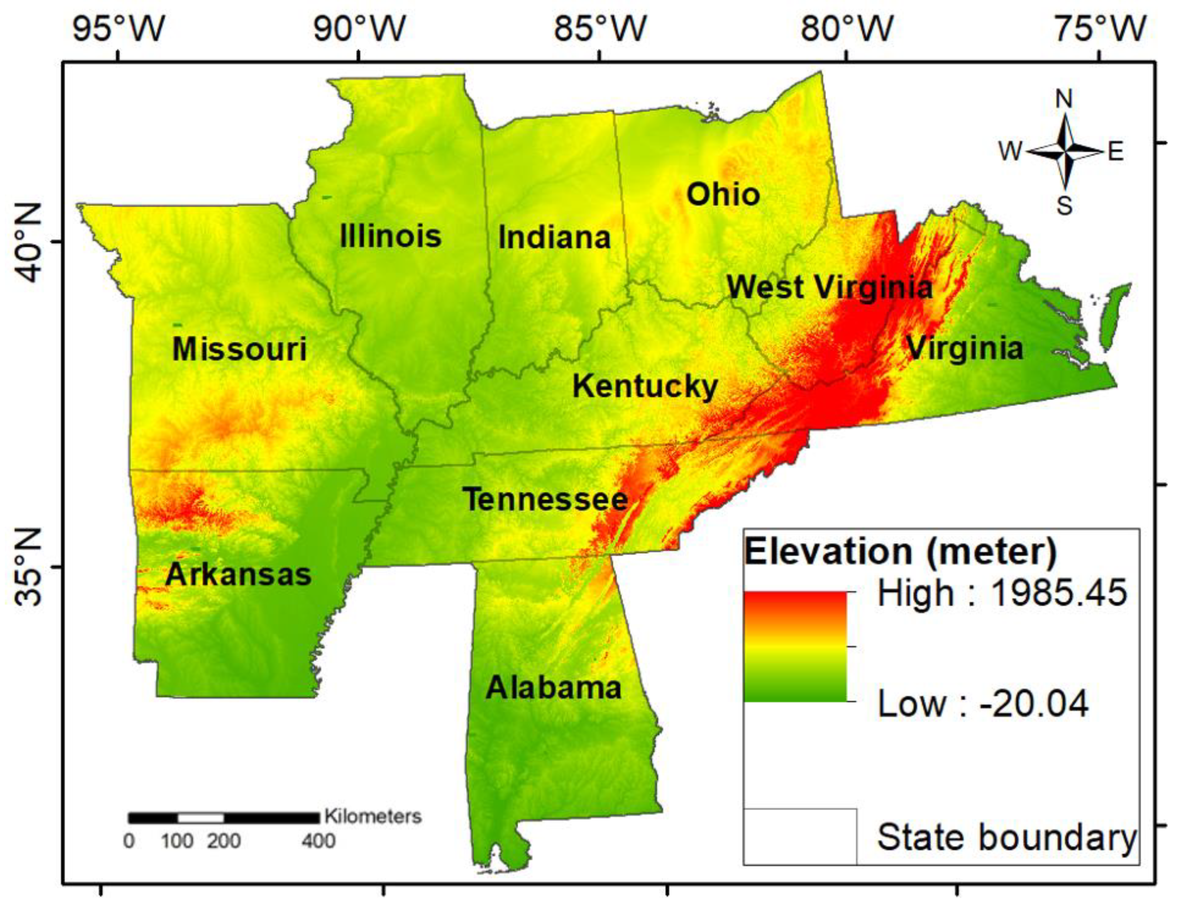
Figure 2.
CART partition of WOM rate from 1998 to 2019. Nodes are indicated in a balloon shape. Each node denotes the mortality rate percentage and the predicted value for the WOM rate (m2/ha/year). Variables that partition nodes are shown between node partitions.
Figure 2.
CART partition of WOM rate from 1998 to 2019. Nodes are indicated in a balloon shape. Each node denotes the mortality rate percentage and the predicted value for the WOM rate (m2/ha/year). Variables that partition nodes are shown between node partitions.
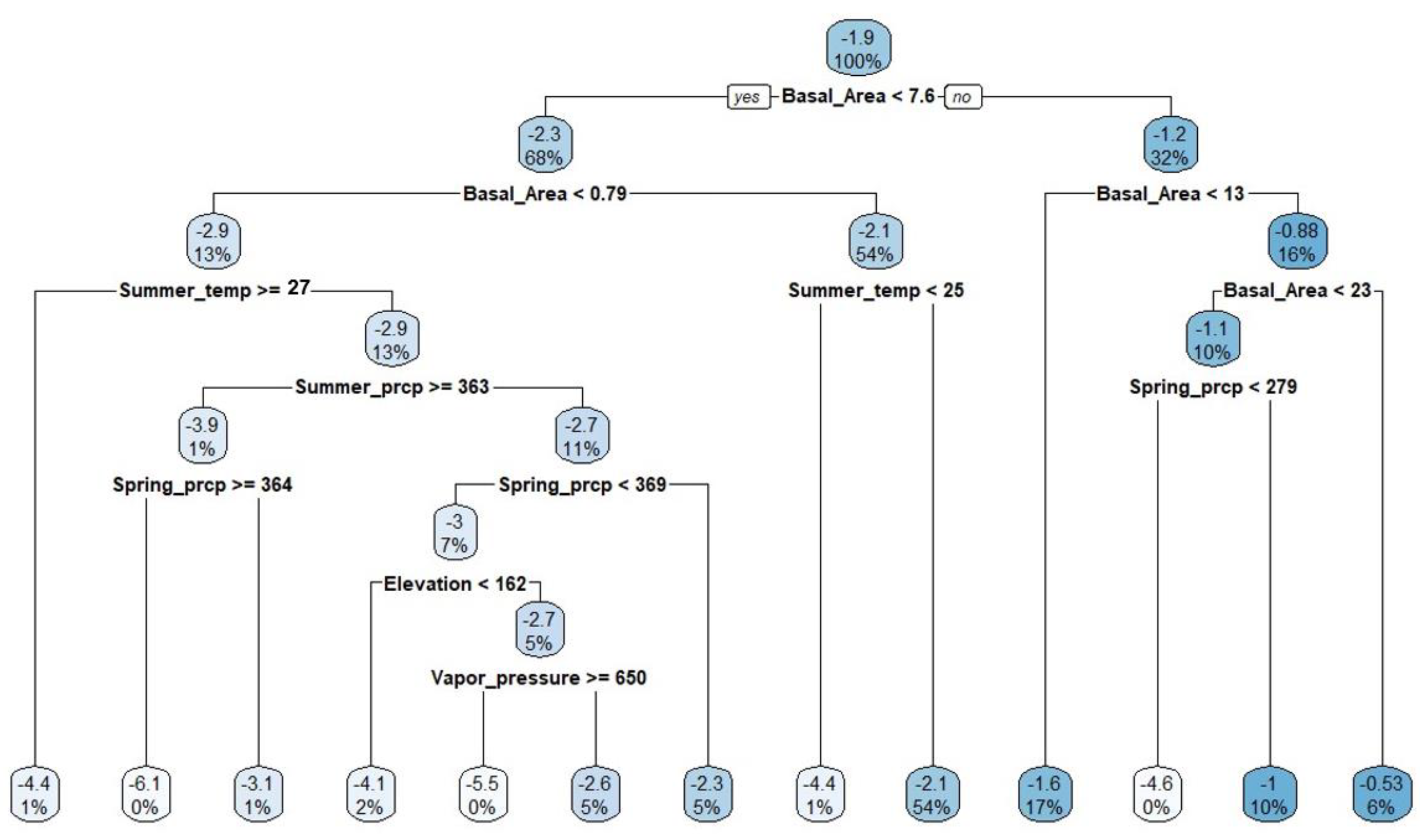
Figure 3.
Showing hierarchical score of variable importance of both biotic and abiotic variables affecting WOM rates. (Note: temp represents temperature, prcp represents precipitation, PDSI represents Plamer Drought Severity Index, Subsoil_C represents subsoil carbon, TopsoilC represents topsoil carbon, and OM represents soil organic matter percentage).
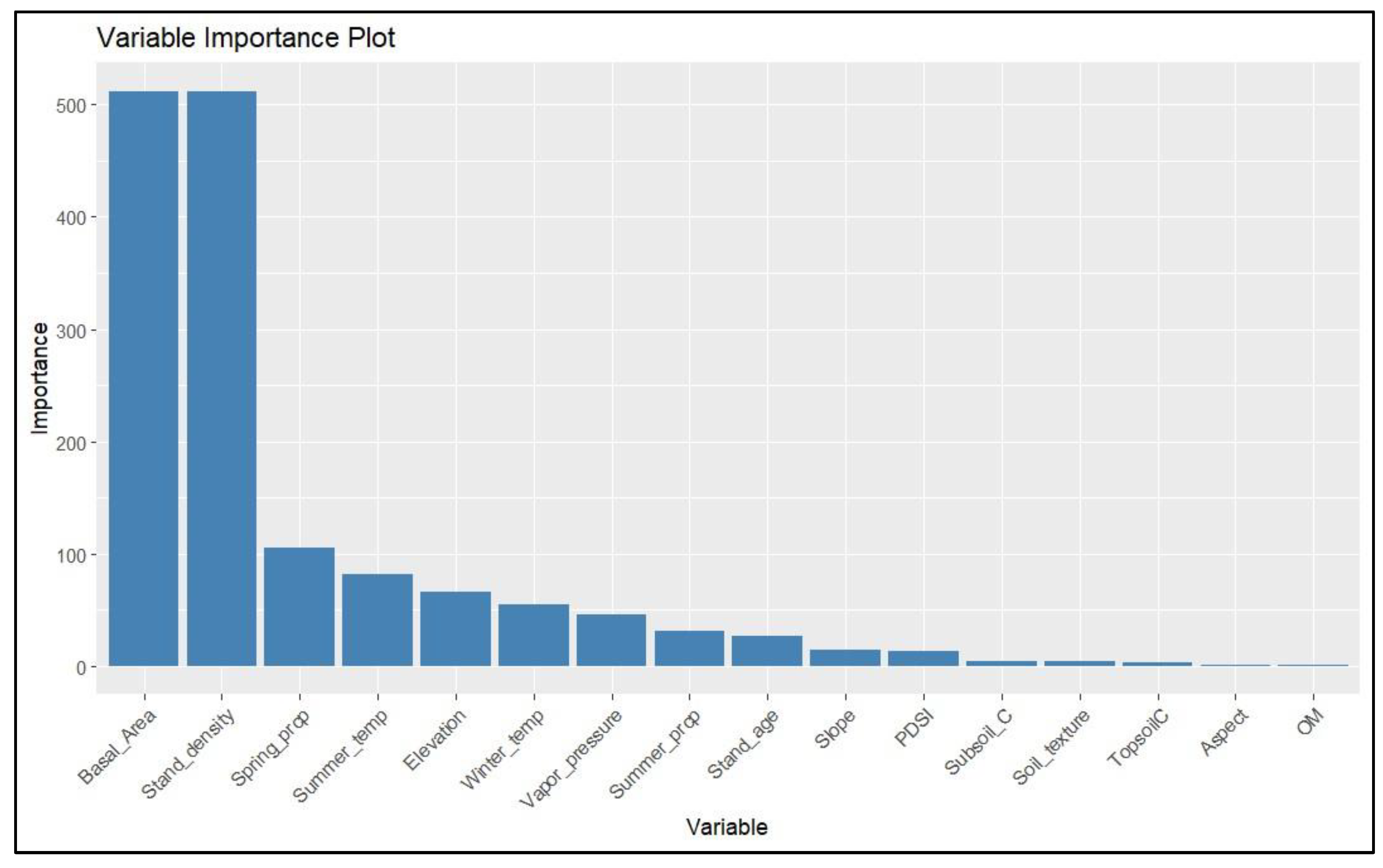
Table 2.
Soil texture with symbols, soil organic matter (SOM%), and total available water (TAW%) classification across the eastern U.S.
Table 2.
Soil texture with symbols, soil organic matter (SOM%), and total available water (TAW%) classification across the eastern U.S.
| Soil Texture | SOM (%) | TAW (%) | ||
|---|---|---|---|---|
| Clay (C) | Loam (L) | Sandy Loam (SL) | No (0) | Very Low (0 - 20) |
| Clay Loam (CL) | Loamy Fine Sand (LFS) | Silt (SI) | Low (0.01) | Low (21 - 40) |
| Coarse Sand (COS) | Loamy Sand (LS) | Silt Loam (SIL) | Medium (0.02 -0.03) | Medium (41 - 60) |
| Fine Sand (FS) | Sand (S) | Silty Clay (SIC) | High (0.04 -0.1) | High (61 - 80) |
| Fine Sandy Loam (FSL) | Sandy Clay (SC) | Silty Clay Loam (SICL) | Very High (1.1 -3.7) | Very High (81 - 100) |
| Inland Water (WR) | Sandy Clay Loam (SCL) | Very Fine Sandy Loam (VFSL) | ||
Disclaimer/Publisher’s Note: The statements, opinions and data contained in all publications are solely those of the individual author(s) and contributor(s) and not of MDPI and/or the editor(s). MDPI and/or the editor(s) disclaim responsibility for any injury to people or property resulting from any ideas, methods, instructions or products referred to in the content. |
© 2025 by the authors. Licensee MDPI, Basel, Switzerland. This article is an open access article distributed under the terms and conditions of the Creative Commons Attribution (CC BY) license (http://creativecommons.org/licenses/by/4.0/).
Copyright: This open access article is published under a Creative Commons CC BY 4.0 license, which permit the free download, distribution, and reuse, provided that the author and preprint are cited in any reuse.


