Preprint
Article

This version is not peer-reviewed.

Title Blockiness of 3D Fractured Rocks of Different Fracture Persistence, Spacing, and Orientations

Submitted:

30 January 2025

Posted:

30 January 2025

You are already at the latest version

Abstract

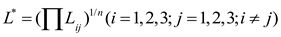
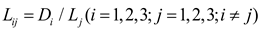
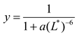
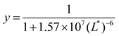
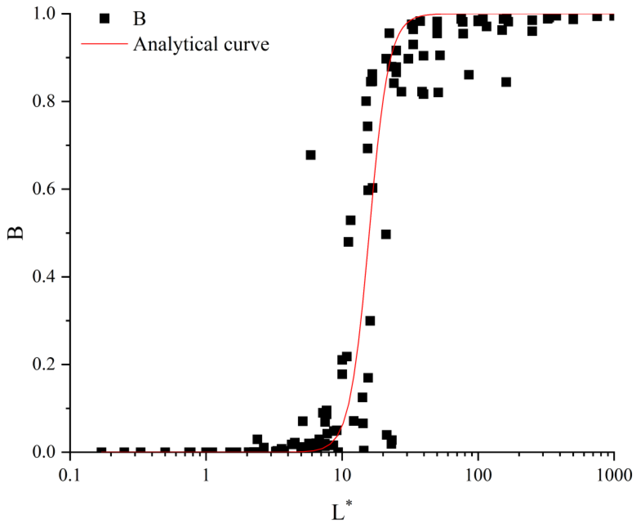
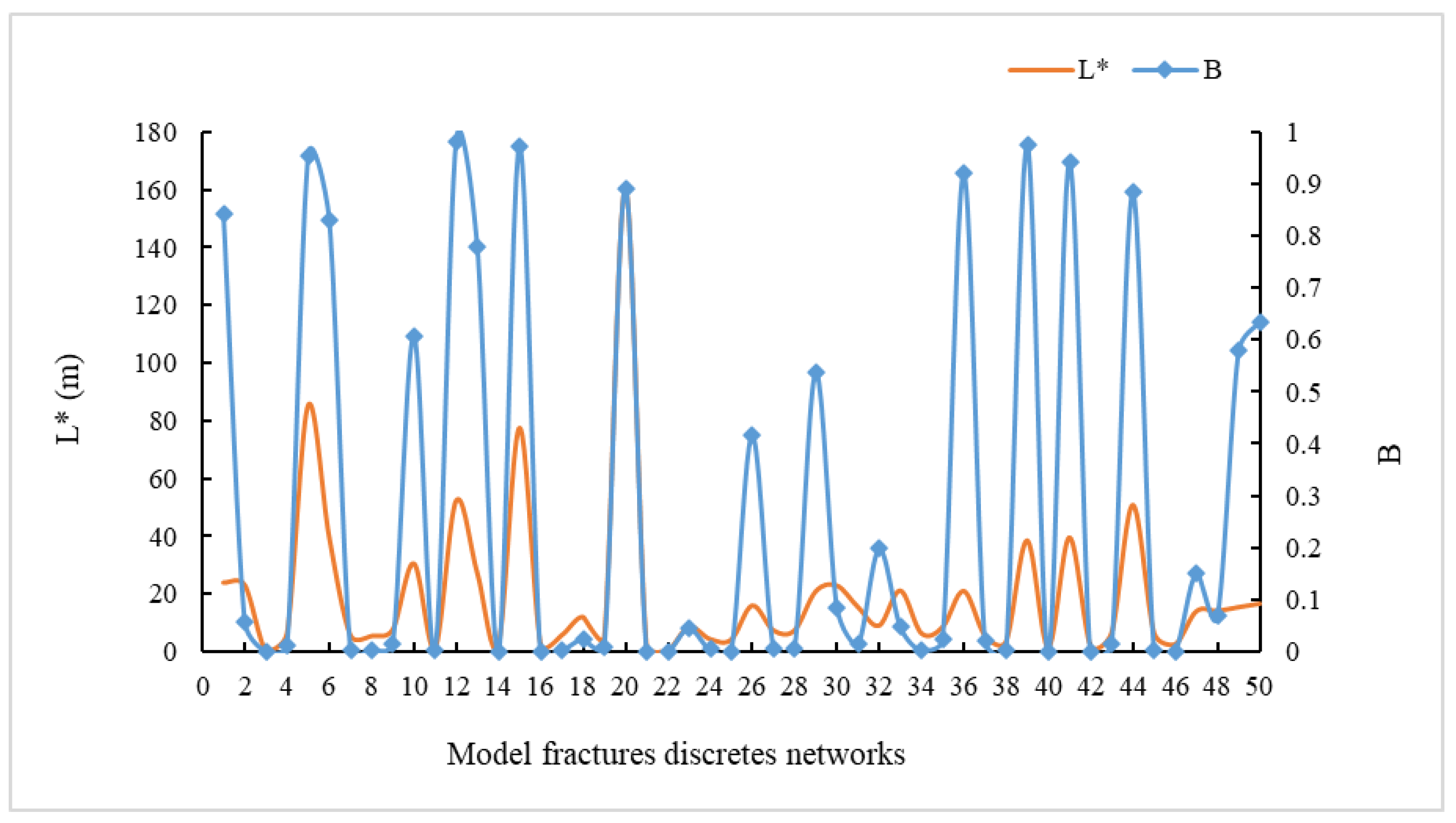
Understanding the blockiness of 3D fractured rocks with varying fracture persistence, spacing, and orientations is essential for comprehending rock mass behavior, particularly in engineering and geological applications. These factors significantly the mechanical behavior, stability, and blockiness of fragmented rock formations. This study aims to analyze the complex behavior of fractured rocks within blockiness fracturing setups using advanced numerical experiments. This study significantly enhances our understanding of how persistence and spacing affect fractured rock formation in three dimensions. Unlike previous studies, our work establishes a fundamental link between fracture geometry and blockiness using parameters of Discrete Fracture Networks (DFNs). Through meticulous analysis and advanced digital experiments, the GeneralBlock software was used to identify and discuss the key components of rupture systems, such as blockiness and representative elemental volume (REV). By establishing DFNs with different parameters, we discovered a fundamental link between fracture geometry and blockiness. The findings indicate that fractured rocks exhibit varied behaviors depending on the blockiness percentage and structural parameters. A higher fracture persistence, lower spacing, and larger angles, limited by the orientation of the fracture surfaces, result in higher L* values. When L* was less than 7.36, blockiness was below 1%. When L* ranges between 7.36 and 22.83, blockiness undergoes a sudden change ranging from 1% to 90%. When L* exceeds 22.83 and the blockiness surpasses 90%, it gradually stabilizes. These findings are crucial for a better understanding and prediction of the mechanical behavior, stability, and blockiness of fragmented rock formations, with significant implications for engineering and geological applications.

Keywords: 
;  ;  

1. Introduction

Rock masses are defined as a collection of blocks of varying dimensions, material discontinuities, stratification surfaces, junctures, and fractures [1]. The impact of persistence, spacing, and occurrence on 3D fractured rock blocks is a complex topic in rock mechanics that significantly affects the behavior and stability of rock masses. Areas known as fractured rock masses initiate, propagate, and merge with macrofractures, leading to the formation of falling rock blocks [2]. Engineers commonly observe this phenomenon, which is attributed to excavation processes [3] and the rearrangement of the geostatic pressure during excavation [4]. The presence of fractured rock masses poses significant challenges in the construction of road infrastructure, tunnel engineering, and drainage channels for water networks, owing to the substantial displacement of the surrounding rock [5]. Understanding fractured rock masses requires assessing the impact of joint persistence and spacing, as these factors form the basis of the continuous-medium method. The analysis of rock block persistence and spacing is fundamental to characterizing fractured rock masses, as the geometry and dimensions of fractures exhibit significant variability. Joint persistence, defined as the extent to which joints propagate within the rock mass, along with their spatial orientation and spacing, critically influences the block size and configuration of the fractured rock mass. Although it has been known for a long time that joint persistence is a key factor in determining the overall integrity of rock formations, most current rock mass classification systems do not take this into account [6]. Therefore, understanding rock fragmentation relies on the presence of fractures of different sizes within the rock formations.
Numerous indices, some of which are commonly used, such as Rock Quality Designation (RQD) [7], Volumetric Fracture Frequency (Jv), and degree of integrity of the rock mass (Kv) [8], are suitable for quantifying the fracturing extent of a rock mass. Over time, several drawbacks have been highlighted for three frequently utilized indices: (1) impersistent discontinuities are disregarded in the Jv technique, (2) The RQD values are anisotropic, and (3) Kv is subject to other factors [9]. The primary criticism also lies in the fact that these three indices focus solely on discontinuity densities, ignoring the impact of discontinuity persistence, and failing to fully account for the geometric features of discontinuities. According to a study by Kim et al. (2007) [6], discontinuity persistence has an effect that should not be ignored, even if the discontinuity density is the main factor that determines the mechanical characteristics and jointing degree of the rock mass [10]. Xia et al. [11] proposed the concept of blockiness (B), which quantifies and classifies the fracturing extent of a geological formation from the standpoint of block size number in response to the somewhat unsatisfactory nature of the current indices. In addition, the concentration, perseverance, and arrangement of discontinuities are all completely considered and organically integrated into the three-dimensional blockiness concept.
In recent research, the characterization of blocks has been used as an index to categorize the quality of rock masses in recent research. Accurate quantitative analysis of the structural properties of discontinuous surfaces in rock masses is an important challenge for accurately characterizing the structural integrity of rock formations. The fundamental nature of cleavage plays a crucial role in the degree of dispersion of geological formations as they are cut into separate blocks. The fracture persistence, density (spacing), number of groups, number of groups, and orientation of fractures in engineered rock bodies are the main factors influencing the geometric characterization of fractures. In A research study, 77 models were developed for fractured rock formations based on seven fracture-dimension classes and 11 spacing classifications suggested and categorized by the International Society for Rock [12]. The impact of fractures on blockiness is widely acknowledged, particularly about fracture spacing, size, and statistical distribution [13,14,15]. Rock masses exhibit a wide range of fracture sizes and distributions [11,16]. Fracture spacing and size play pivotal roles in regulating the size, number, and strength of blocks.
This study aims to analyze the identification and composition of rock blocks. Nine iterations were conducted for scope size to minimize the effects of random variations. Additionally, the quantifiable correlation B, fracture interval, and fracture dimension were investigated by assuming equal fracture dimensions, as proposed by Xia and Yu in 2020 [2,11]. The measure of variability was used to indicate the level of dispersion of fracture proportions. Blockiness calculations were performed using the GeneralBlock software, which is capable of analyzing the influence of the fracture geometry parameters on B and REV. The probability of random errors in this relationship was minimized by conducting multiple calculations. This process involved the following steps: 1) Generate the three-dimensional discrete fracture model fracture size, 2) evaluate the blockiness of different fracture formations, and 3) evaluate the effects of persistence, spacing, and orientation on the blockiness of three-dimensional fractures.

2. Generation of Three-Dimensional Discrete Fractures

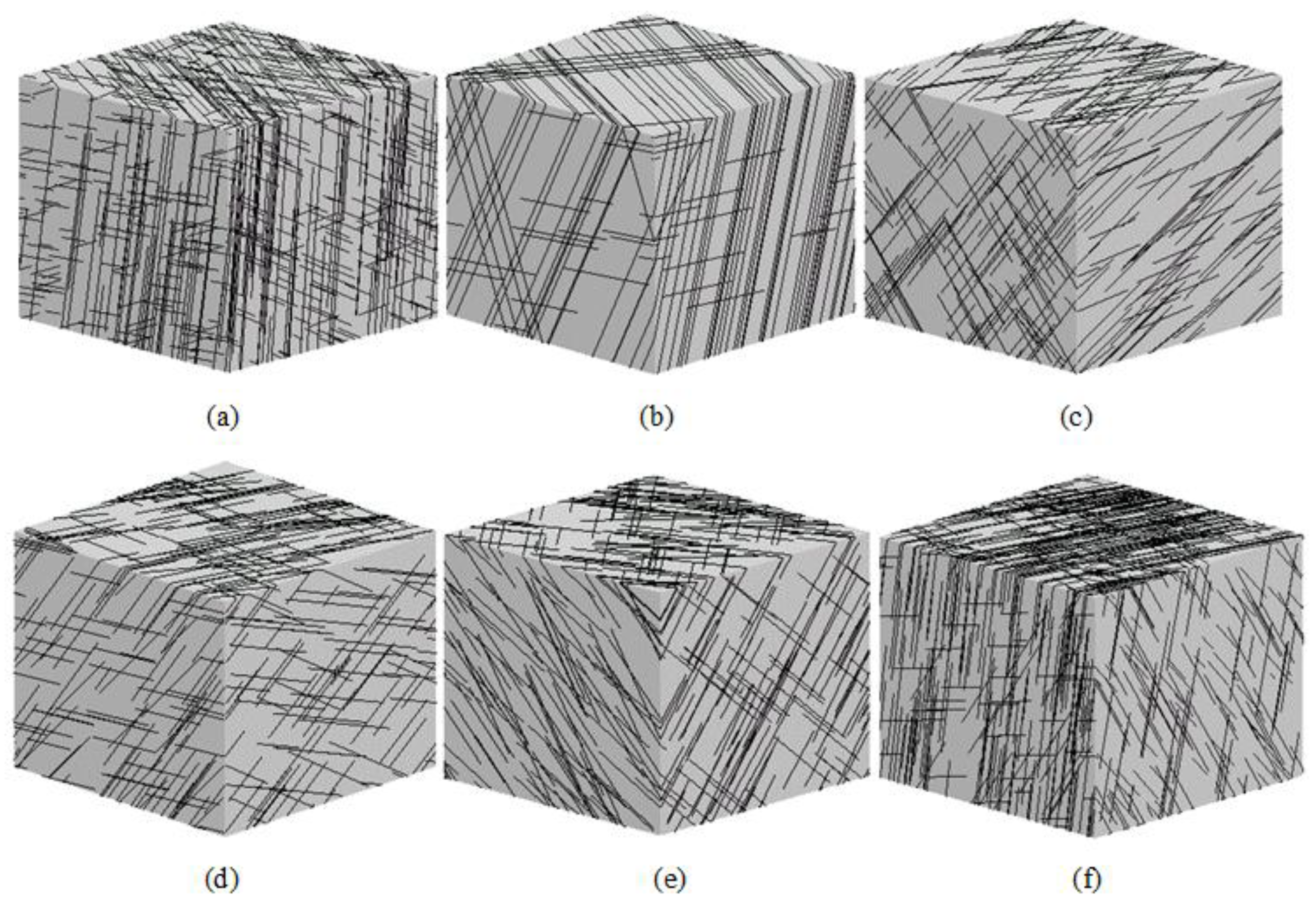
2.1. Generation of Three-Dimensional Discrete Fractures

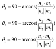
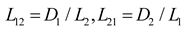
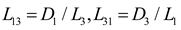
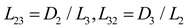
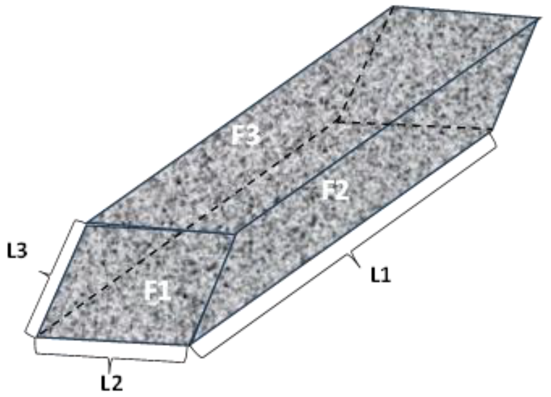
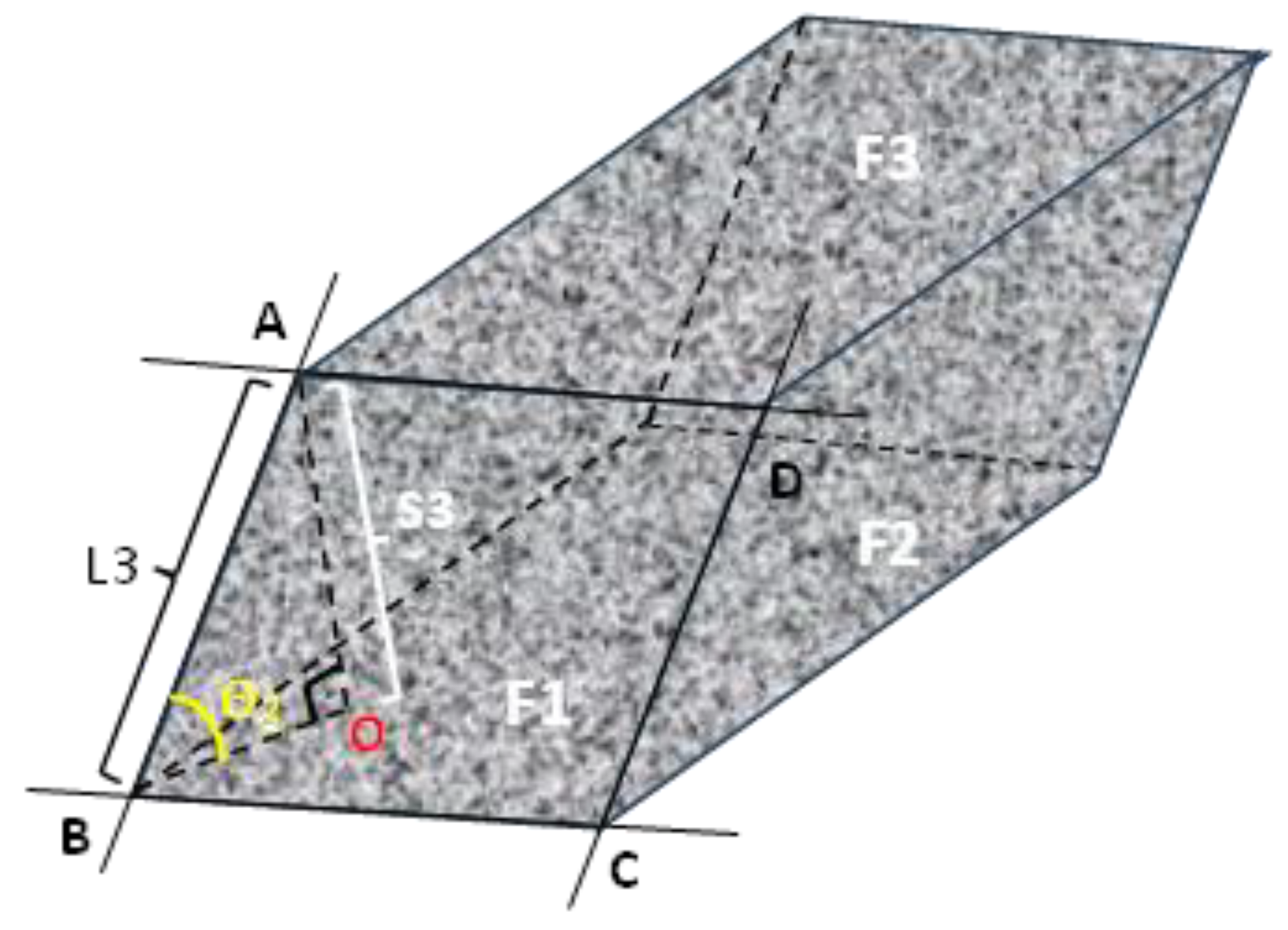
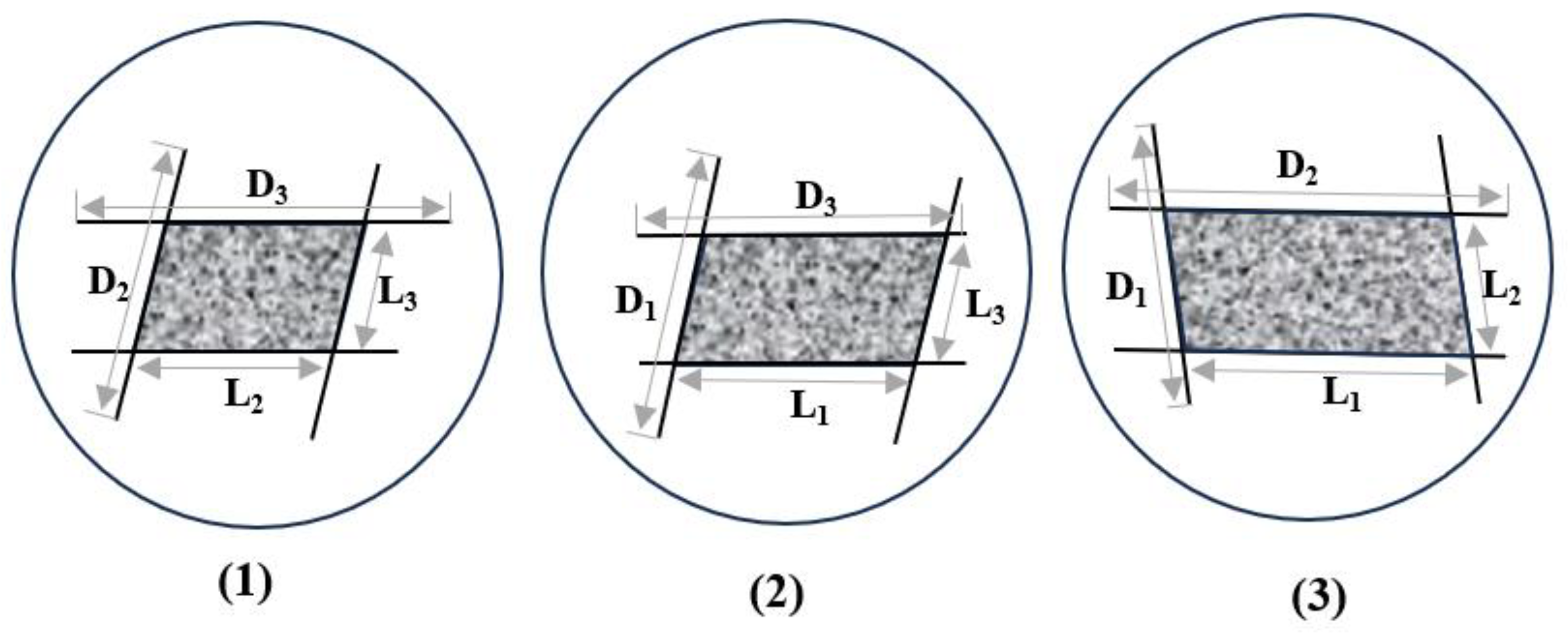
2.2.1. Fracture Geometry Parameters

To accurately simulate rock mass structures and faithfully reproduce the natural appearance of field fractures, constructing fracture models that approximate real-world arrangements is crucial for precisely describing the basic elements of fractures, which is a major challenge in the study of rock mechanics. Field observations can capture only the exposed shapes of rock fractures, resulting in limited data availability. Therefore, mathematical methods are typically employed to reconstruct fracture shapes, assuming fracture parameters to be random variables to characterize the stochastic network features of fractures. Describing the developed fracture features within rock masses and constructing three-dimensional spatial models of fractures requires determining parameters such as the spatial position, morphological characteristics, and attribute features of fractures.
Fracture networks can be more accurately represented in numerical models and engineering evaluations using GeneralBlock software. Fracture persistence and spacing are two key factors that affect the size of the geologic formation mass and determine whether it functions as a discrete or an uninterrupted continuum. In contrast, fracture yield affected the shape of the geological formation. Consequently, we focused on the variables of fracture persistence, spacing, and orientation to investigate their effects on fractured rock mass size and REV presence.
To identify rock blocks, representative rock-mass models must be established. By controlling for other variables, the impact of varying the fracture width and spacing on the blockiness of rock formations can be systematically evaluated.
ISRM (1978) [17] classified fracture persistence and spacing into five and seven rates, respectively. The classification of the fracture persistence is listed in Table 1, and the fracture spacing is listed in Table 2. The recommendation provided by the ISRM is considered sufficiently comprehensive to form a foundation for generating various discrete fracture networks (DFNs). The proposed categorization for fracture persistence and spacing can be utilized to model rock masses exhibiting different structural characteristics, ranging from solid to fractured, in a methodological manner.
When constructing 3D fracture network models, it is essential to address the complex variations in fractures in the 3D space. Researchers have employed various shape assumptions in fracture models such as circular, elliptical, and regular polygonal geometries. However, most theoretical studies and practical applications favor simplifying fractures as disks, as illustrated by Long et al. [11,16,18,19]. In this model, the fracture was considered to be a flat surface with uniform persistence across all directions. Thus, the shape of a fracture can be described by its diameter or radius. If data on persistence and spacing are available, the three-dimensional density (d3) of the disc fractures can be calculated using Equation (1). Based on Table 1 and Table 2, we improved and extended the classification system for integrated system monitoring, and calculated the 3D densities, as shown in Table 3.
Preprints 147744 i001
In this context, d1 (1/m) represents the linear density of the fracture and E(D2) denotes the mean value of the square disk diameter. Table 3 lists the three-dimensional density of the 84 fracture types, refined according to ISRM classification recommendations, and are presented in the table below.

2.2.2. Fracture Network Modelling

Fractured rock bodies have complex geometric features such as different orientations, lengths, and spacings, and different combinations of these geometric parameters form a complex fracture network within the rock body. Characterizing and analyzing fractured rock masses can be effectively accomplished using fracture network modelling, especially when the DFN approach is applied. It offers insightful information on the behavior, connectivity, and fragmentation of rock masses. Different patterns are present in the cleavage network of rocks, the most common of which are three sets of orthogonal or semi-orthogonal cleavages [20]. In this study, Monte Carlo methods were used to randomly sample fracture persistence, spacing, and orientation based on the fracture disc assumption, using the fracture parameters and the probability density distribution function they obey [21]. Finally, 50 groups of 3D random fracture networks were generated using a computer with the following fracture network parameters (Table 4).
The dimensions of the representative elementary volume (REV) for rock can be appropriately expressed as a multiple of the fracture spacing, typically ranging from two to 20 times this spacing. To ensure that the fracture network’s generation range exceeded the study area’s size without boundary effects, we defined the fracture network’s generation area as a cube with dimensions L×L×L. This specific relationship can be represented as follows:
L = 40S*+Dmax
S* = (ΠSi)1/3 (i=1,2,3)
Dmax = max (D1, D2, D3)
In this context, S* represents the geometric average of the spacing between the three groups and Dmax denotes the highest persistence value observed across these groups. Figure 1 shows the six representative rift models.
Theoretically, when the range is limited, the blockiness percentage exhibits greater variation. As the range of the model expands, the blockiness percentage tends to stabilize. This was because the three-dimensional fracture density within the simulated rock mass area remained constant. Consequently, a smaller rock mass range encompasses fewer fractures, whereas a larger range incorporates more.

3. Blockiness Analysis and REV Size Estimation of Various Fractured Rocks

3.1. Blockiness of Fractured Rock Mass

Fractures are complexly interconnected within a fragmented rock formation, causing the rock mass to be segmented into multiple, relatively autonomous rock units. The rock mass integrity index provides a quantitative measure of the overall structural stability of a rock formation, which is largely determined by how the fractures within it are interconnected. Specifically, a higher fracture connectivity indicates more extensive fracture development within the rock mass, resulting in greater deterioration of its structural integrity.
The scientific community has developed numerous evaluation systems to measure the deterioration of rock mass integrity owing to fractures. Among these methods, rock quality designation (RQD) has emerged as a widely accepted classic approach.. However, these traditional metrics have revealed certain limitations in practical applications, especially the RQD values, and because of their inherent directional sensitivity, it is often difficult to comprehensively capture the subtle fractures that have poor continuity but are numerous in number, and thus may underestimate the actual impact of fractures on rock mass integrity. Three-dimensional discrete fracture network (DFN) modeling has emerged as a popular research area owing to its ability to capture the three-dimensional structural features and integrity of fractured rock masses more accurately. Traditional integrity evaluation metrics, such as RQD, appear to be inadequate because it is difficult to adequately describe and quantify the intricacy and dynamics of the fracture network in a 3D space.
The term “blockiness” refers to the extent to which a rock mass is composed of distinct blocks. This characteristic significantly influences the stability and mechanical properties of rock masses [21]. The blockiness level was determined by assessing the quantity and size of the blocks within the rock mass. A high degree of blockiness suggests extensive jointing in the rock mass, indicating that it should be treated as a discontinuous medium and vice versa. In this context, the block percentage serves as an indicator of blockiness, and is used to quantify the extent of jointing in the rock mass. This percentage was calculated as follows.
Preprints 147744 i002
In this equation, V represents the overall volume of the rock mass and Vi denotes the volume of an individual block i. Variable n indicates the total number of blocks present in the rock mass.

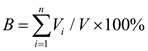
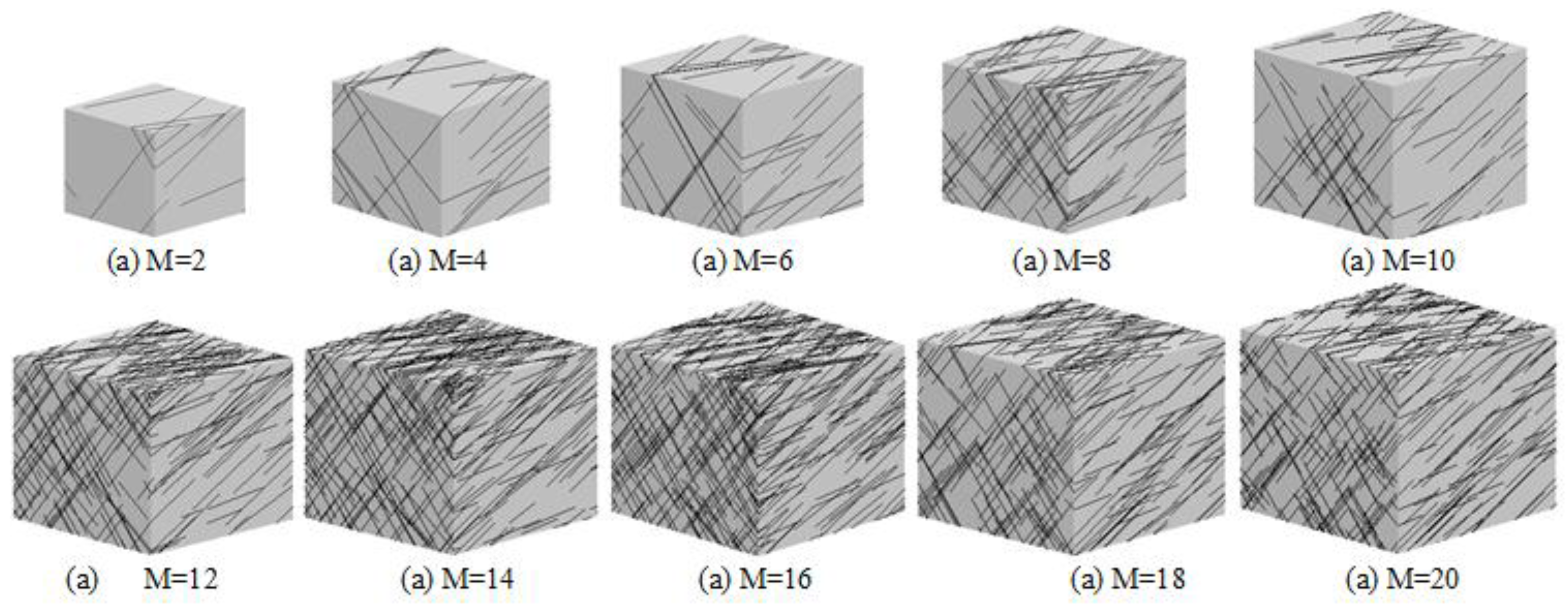
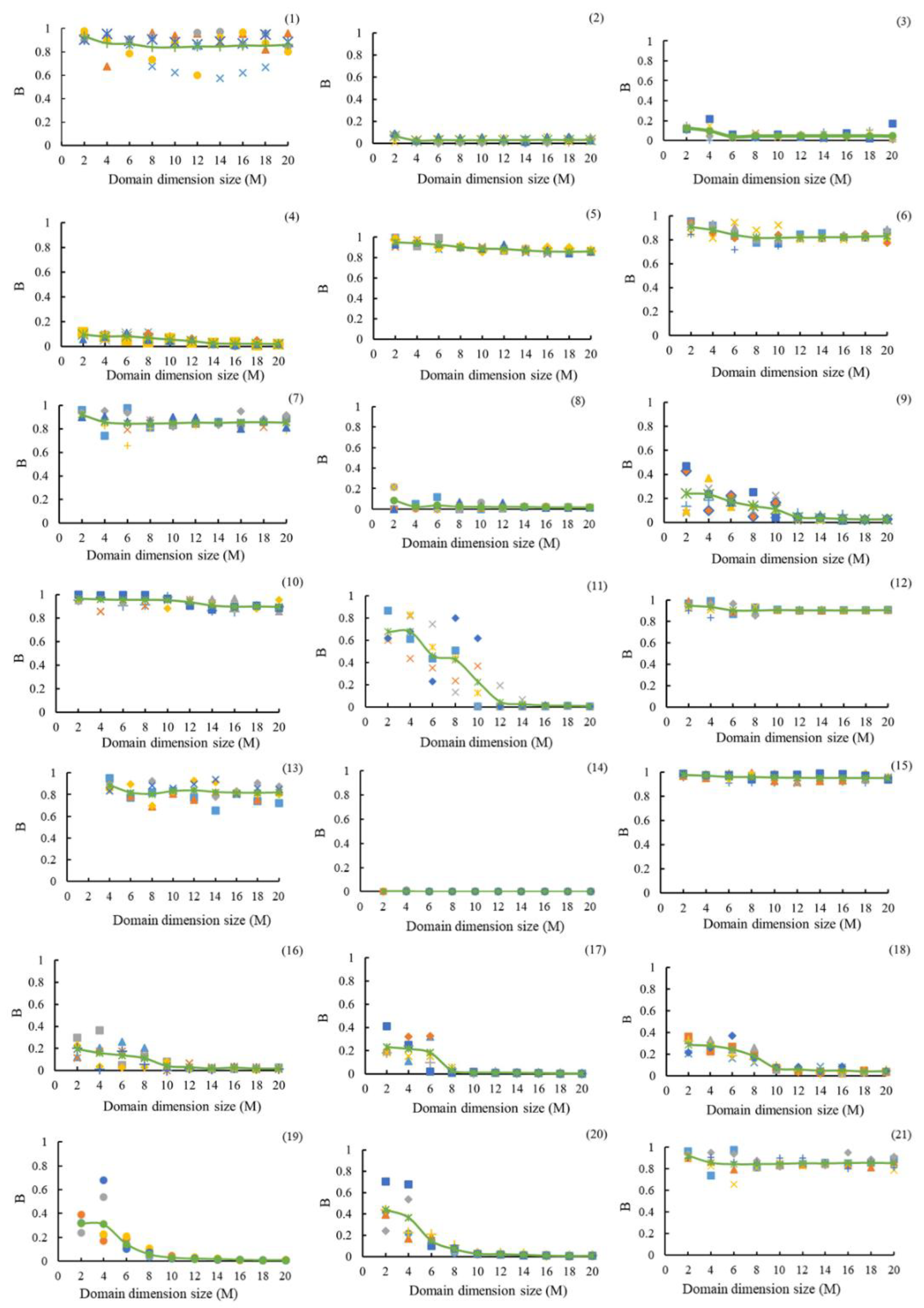
3.2. Estimation of the Blockiness and REV

Effective cleavage, which creates key blocks, can significantly affect the stability of the rock masses. This process can result in various hazards, including rockfalls and landslides. We can forecast potential rock mass stability issues by analyzing the extent of division of a rock mass into separate blocks. Figure 2 illustrates the fractured rock mass model employed to compute different blockiness levels. The range of the model for each rock mass was chosen to be 2–20 times the spacing, demonstrating how the rock mass structure changes when different ranges are selected for the structural model. At the model level, the number of generated fractures ranged from 9 to 523 (Figure 2). The illustration clearly demonstrates that smaller models have fewer crack networks, whereas larger models exhibit an increased number of crack networks.
The number of fractures influences the degree of fragmentation in a rock mass, which varies considerably across different geological settings. The model was run several times for each domain size to mitigate the effect of randomness.
The relationship between blockiness and area size is illustrated in Figure 3, which depicts the relationship between B and area size across 12 representative models. The vertical axis represents the blockiness, whereas the horizontal axis shows the domain size. The domain sizes were varied from 2 to 20 times the fracture spacing, with the plotted curve representing the average of nine random iterations.
As illustrated in Figure 3, the principle governing rock mass blockiness follows the same pattern as that controlling porosity, a concept previously explored by Bear. Applying these rock mass models to small volumes often results in significant fluctuations in the blockiness. We identified the REV as the volume at which blockiness stabilized to a constant value. Any noticeable variations in blockiness beyond the REV indicate heterogeneity in the medium. This study assumed that the model cracks were evenly distributed and that blockiness would persist at volumes larger than the REV. In the past, researchers examined how properties change in porous media using both real rocks and numerical models of rocks of different sizes. These studies have examined different properties, rock types, measurement methods, and sample dimensions. Multiple researchers [21,22,23,24,25] have determined that the coefficient of variation (Cv) is an effective measure for quantifying variability across different sample volumes with multiple iterations. A representative effective property was established when Cv fell within the homogeneous range (0 < Cv < 0.5) and the corresponding sample volume approximated the Representative Elementary Volume (REV). Nordahl et al.[26] introduced a method for estimating REV in realistic geological models that explicitly incorporate heterogeneities.
When the fracture spacing increased fourfold, the block percentage in nearly all rock masses underwent substantial change. Nevertheless, rock masses with higher density and extended fracture lengths maintained a consistent block percentage. When the search range was 10, the degree of blockiness in almost all rock masses began to stabilize, aligning with the fracture spacing level.
If the fluctuation range of the block degree was set as the point where it did not exceed 20%, it was considered the stability starting point, and the search range length at this time was designated as the representation unit. Regarding body size, it can be preliminarily assumed that from a swelling degree perspective, most REV fracture rock masses have a size range of 8–18 times the spacing.
The representative elementary volume (REV) for each model was determined as the volume at which the coefficient of variation (CV) fell below 0.5. Both the measured permeability (both vertically and horizontally) and the correlation lengths of the lithological elements affected the size of the REV. We used the average and variance of blockiness values to assess convergence, whereas Cv quantified the variability across nine random realizations. The blockiness values of the nine realizations required a standard deviation of less than 50% of their mean. The domain size for the calculations can be defined either as mentioned above or as the REV size. The minimum REV was identified as the smallest domain size that satisfied these criteria.
The blockiness and REV for the 50 anisotropic rock mass types listed in Table 4 were computed, and the results are presented in Table 5. The blockiness of each DFN was established when the domain size was 20 times the fracture spacing. We determined the blockiness values for all the 50 anisotropic DFN types. The curve in the figure depicts the average of each calculation outcome. In certain rock mass models, the extent of the rock mass ranges from 8 to 20 times the interfracture spacing.
The degree of blockiness in the fractured rock masses can be assessed using the REV volume, as indicated in Table 5. The analysis revealed that six blockiness values were above 90%, three fell between 80% and 90%, three ranged from 50% to 70%, six were between 10% and 60%, 11 were between 1% and 10%, and the remaining 12 were at 0%. When the blockiness value approaches 100%, it suggests that the rock should be considered a collection of separate blocks. Conversely, a blockiness value near 0% indicates that the rock has good structural integrity.
We found that angle, distance, and length significantly influence the representative elemental volume (REV) and bulk effects in soils and rocks. Determining the REV and comprehending huge impacts require consideration of the length, angle, and distance. These factors have a direct impact on stability; therefore, they must be carefully considered.

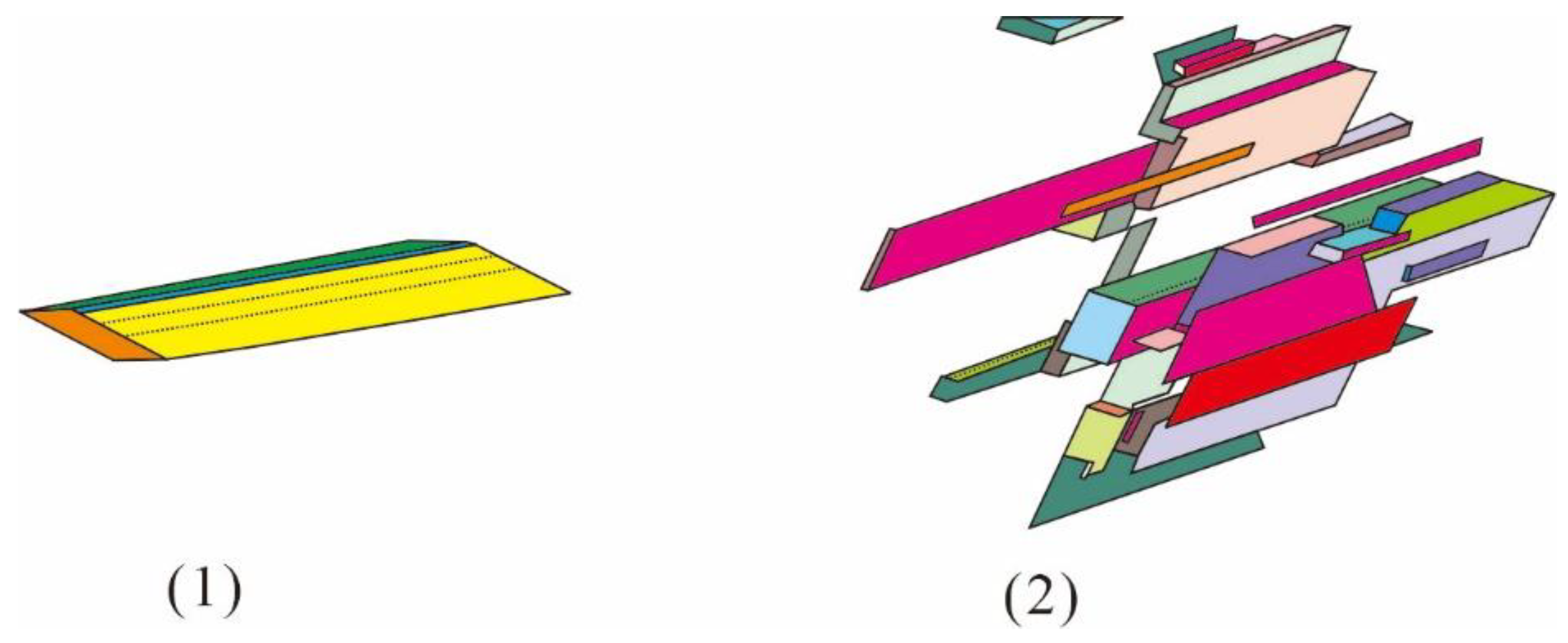
4. Two Types of Fractures that Result in Block Formation

Fracture cutting is a critical process in materials science and engineering and is fundamental for generating a variety of geometric shapes. This study delves into two distinct block shapes that emerge as a result of the fracture cutting. Fracture cutting occurs when a tool or sharp edge penetrates the material, inducing plastic deformation and causing the material to shear along the rake face of the cutting edge [27]. This can result in two primary block formations: radial and shear-type fractures. Radial cleavage fractures originate within the cylinder wall and extend outward to the surface, whereas shear-type fractures occur independently and serve as an energy-dissipation mechanism within the inner portions of the cylinder wall [15]. The formation and propagation of these fractures are strongly influenced by factors such as the wall thickness of the workpiece, the applied loading conditions, and the microstructural properties of the material. Microstructural analysis of the fractured cylinder segments showed a clear connection between the type of fracture and degree of grain boundary distortion. Furthermore, significant shock twinning was noted in the fragments, and the grain structure near the boundary between the fracture surface and untouched material displayed distinctive patterns [28]. The ability of a fracture to produce a block is affected by its length-to-spacing ratio. In rock masses where this ratio is low or where fractures are closely spaced, the random fractures generated by a discrete fracture network model may not fully separate the rock mass into independent blocks. Although some fractures possess a strong cutting capacity, resulting in separate blocks (Figure 4a), others, owing to their spatial arrangement or other constraints, form aggregates of blocks rather than distinct units (Figure 4b). Most natural rock formations exist between the extremes of the continuous media and isolated block systems. Fractured rock masses frequently contain both independent and blocky aggregates. Consequently, this study provides two separate B-value fitting formulas, one for complete cutting and the other for incomplete cutting, and identifies the most suitable fitting approach.

5. Effects of Spatial Heterogeneity and Alignment on the Blockiness of 3D Fractures

The anisotropic fractured rock mass is divided into three groups based on ductile spacing and fracture occurrence, which differ. The rock mass is divided into segments by interconnected fractures, and the size and form of these segments are influenced by factors such as fracture tendency, angle of inclination, spacing, and length, as well as a more fragmented rock mass resulting from a higher degree of fracture connectivity. The blockkiness effectively gauges the quality and stability of a rock mass. Overall, blockiness is a key metric for analyzing and classifying fractured rock masses. This is determined by how these variables interact with each other in complex ways.
Solid materials, such as rocks or the Earth’s crust, can develop natural fractures due to external pressure. Three groups of principal stresses, represented by fractures 1, 2, and 3, intersect the rock body after it has formed, as shown in Figure 5. Although rocks are typically subjected to three stress-cutting directions, the main stress sets found in nature are not always perpendicular to each other. The accompanying image illustrates how the angles between the primary stresses influence the shape of the rock mass created by intersecting cleavage surfaces. The presence of fractures is a crucial factor for determining whether a rock can be cut into blocks. The size and quantity of the blocks extracted from the fractured rock mass are determined by the fracture persistence and spacing, while the fracture inclination angle dictates whether the resulting rock mass is a cuboid or an oblique prism. Additionally, the relationship between fracture persistence and the length of the intersection between the fracture surfaces can indicate whether the fracture is completely severed.
L3 can also be considered as the length of the edge formed by the cutting of fractures 1 and 2. To visualize and understand the complex three-dimensional geometry of fragmented rock formations, refer to Figure 6. Whether fracture 1 can fully connect the two adjacent fracture surfaces of fracture 3 can be determined by calculating the ratio of the ductility of fracture 1 to L3.
The lengths L1, L2, and L3 of the intersecting lines between fracture surfaces 1, 2, and 3 cut by another fracture were calculated as follows:
Preprints 147744 i003
It was necessary to determine the values of L1, L2, L3, θ1, θ2, and θ3. We consider the normal vectors of fracture surfaces 1, 2, and 3 as n1, n2, and n3, respectively, where n1=(a1,b1,c1), n2=(a2,b2,c2), and n3=(a3,b3,c3). The direction vector of the intersection between fracture surfaces 1 and 2 is denoted as m3=(e3,f3,g3), whereas the direction vector of the intersection between fracture surfaces 1 and 3 is represented as m2=(e2,f2,g2). The direction vector of the line formed by the intersection of fracture surfaces 2 and 3 is m1=(e1,f1,g1). The calculation of m3 was performed as follows:
Preprints 147744 i004
From the above equation, we can introduce the numerical magnitudes of e3, f3, and g3.
Preprints 147744 i005
Similarly, the vector representations of m2, m3 can be obtained, if the normal vector of fracture plane 3 is known to be n3, then the angle θ3 between the intersection line of fracture planes 1 and 2 and fracture plane 3, as well as θ2, θ1, can be obtained
Preprints 147744 i006
A tetragonal column is formed when the generated fracture completely cuts the rock body. The ratio of different rift persistence values to the shortest distance of complete cutting on the rift surface can be observed in Figure 7 (Equations (10)–(12))
Preprints 147744 i007
Preprints 147744 i008
Preprints 147744 i009
The following formula summarizes the six sets of ratios for the three fracture surfaces.
Preprints 147744 i010
The magnitude of the influence of the three factors of ductility, spacing, and yield on the combined influence factor of the level of block mineralization in the case of a fully cut rock body was replaced with the value of L*.
Preprints 147744 i011
The relationship between the blockiness, fracture length, and spacing can be represented by an S-shaped surface in geometric terms. In this study, we aim to develop an analytical formula for this relationship using an empirical approach. Drawing from our analysis and discussion, we introduce an S-shaped analytical equation to illustrate how the massing level correlates with the fracture spacing and ductility of the rock mass. This equation is formulated as follows:
Preprints 147744 i012
L* was fitted to blockiness B to obtain a fitted curve for the blocking level after the rock body was completely cut, as shown in Figure 8.
Using the least-squares method, the parameter in Equation 15 was calculated to be a = 1.57 × 10⁷, based on the lumped body and L* values from 50 classes of anisotropic DFNs and 84 classes of isotropic DFNs. A robust relationship was observed between the lumped body and L*, with a correlation coefficient of R2 = 0.83. Consequently, the following equation was derived:
Preprints 147744 i013
When examining the relationship between B and L*, the rock mass exhibited an S-shaped growth pattern as L* increased.
Research has shown that the presence of a Representative Elementary Volume (REV) is more likely when persistence and spacing are increased and spacing is more compact. However, most of these conclusions have been drawn from studies on uniform fractures, neglecting the diversity in spacing and persistence among different fracture sets within the fractured rock mass. The primary factor influencing the effects of persistence and spacing on the REV is the reciprocal cutoff between the spacing of one fracture set and persistence of another. Figure 9 illustrates the relationship between the fracture plane angle and parameters L* and B.
Some cleavages can form blockiness by cutting each other, whereas some cleavages, even if they have a connection, cannot form blockiness through mutual cuts alone. At this point, the main factor is the assembly of blockiness, which is accompanied by the development of independent blockiness. This is why the level of blockiness changes significantly during this period, from 1% to 90%. This is also why the level of massification fluctuates strongly in this interval, and the level of massification fluctuates between 1% and 90%. In the first stage of blockiness development, when L*<7.36, the fracture cannot cut the rock body to form blockiness or cut blockiness, but cannot be connected to adjacent fractures because of its spatial distribution. L* causes a gradual increase in the blockiness level and B does not exceed 1%. When it is between 7.36 and 22.83, it enters the second phase of the blockiness mutation. At this stage, the cleavages develop progressively and can form blockiness; however, the spatial distribution of the cleavages has a greater impact. Once L* surpasses 22.83, the process enters the blockiness stabilization stage. At this point, the impact of the spatial distribution becomes negligible owing to the high cutting capacity of cleavage. The rock mass was predominantly composed of isolated blocks, and B approached 100%. There are two relatively stable phases of blockiness mineralization levels, and there may be some error in discussing the effect of a single factor, ductility, spacing, and yield, on blockiness mineralization levels within these two stable phases. The relationship between the L* value and blockiness is shown in Figure 9. As the L* value decreased, the connectivity between the cleavage surfaces and the ability to cut each other to form blocks decreased, and the block size class B also tended to decrease.

6. Conclusions

We used the GeneralBlock program to examine the mechanical properties of a broken rock mass with many joint assemblies that stayed together in different ways. The goal of this study was to determine the mechanical behavior of 3D fractured rock blocks by examining the impact of persistence, spacing, and incidence using statistics. We utilized a statistical experimental design tool to create block systems with varying persistence factors, spacings, and joint orientations. This method was used to create networks that are not orthogonal, speed up simulations, and make it easier to choose the input parameter combinations that define the shape of fractured rock masses.
These findings unequivocally demonstrate that spacing and persistence are the key considerations in the design of engineered rock structures. After looking at 50 different fracture groups in a planned way, I came up with a way to fully look at how ductility, spacing, and incidence affect the presence and appearance of REV. Blockiness influences the overall index L*. The GeneralBlock software simulations showed that the REV is more likely to occur in cracked rock masses with high L* values (high ductility, small spacing, and large fracture plane angles) and stable levels of blockiness.
The L* value is a three-dimensional parameter that can be calculated by comparing the persistence of one set of fractures with the spacing of another set of fractures and the angle between the two fractures. It can be used to measure changes in the REV, history of block-level growth, and types of fractured rock mass blocks. When L* was less than 7.36, massiveization occurred slowly and did not exceed 1%. This means that few fractures cross to form masses, which supports the strong integrity of the rock mass. For 7.36 < L* < 22.83, massing exhibited significant sensitivity to variations in L*, with the blocking escalating from 1% to 90%. When L* exceeded 22.83, the body was predominantly segmented into isolated blocks, with blocking values approaching 100%, thereby resembling a collection of discrete blocks.
Three critical criteria substantially affect the dimensions, morphology, and stability of 3D fractured rock blocks, namely orientation, persistence, and spacing. Understanding both their individual and combined effects is important for accurately characterizing rock masses, determining their stability, and designing engineering solutions for a wide range of geotechnical problems. This study conducted a thorough examination of fractured rock masses using these three criteria. Due to the inability to control for variables, individual factors were not analyzed separately. This study did not examine various forms of persistence and gap width distributions, necessitating additional research.

Author Contributions

Conceptualization, K.L.M.; methodology, KLM.; software, K.L.M; validation, KLM., Q.W and Y.L.; formal analysis, K.L.M., and QW.; investigation, K.L.M.; resources, Q.Y.; data curation, K.L.M.; writing—original draft preparation, K.L.M.; writing—review and editing, K.L.M.; visualization, KLM., Q.W., and Y.L.; supervision, Q.Y.; project administration, X.X.; funding acquisition, Q.Y. All authors have read and agreed to the published version of the manuscript.

Funding

Not applicable.

Institutional Review Board Statement

Not applicable.

Informed Consent Statement

Not applicable.

Data Availability Statement

All data used to support this study are included in the manuscript.

Acknowledgments

In this section, you can acknowledge any support given which is not covered by the author contribution or funding sections. This may include administrative and technical support, or donations in kind (e.g., materials used for experiments).

Conflicts of Interest

The authors declare that they have no known competing financial interests or personal relationships that could have influenced the work reported in this study.

Abbreviations

The following abbreviations are used in this manuscript:
DFNs Discrete Fracture Networks
REV Representative elemental volume
RQD Rock quality designation
Jv Volumetric fracture frequency
Kv Degree of integrity of the rock mass
ISRM International society for rock mechanics

References

  1. Riquelme, A.J.; Tomás, R.; Abellán, A. Characterization of Rock Slopes through Slope Mass Rating Using 3D Point Clouds. Int. J. Rock Mech. Min. Sci. 2016, 84, 165–176. [Google Scholar] [CrossRef]
  2. Chen, S.; Qiao, C.; Ye, Q.; Khan, M.U. Comparative Study on Three-Dimensional Statistical Damage Constitutive Modified Model of Rock Based on Power Function and Weibull Distribution. Environ. Earth Sci. 2018, 77, 1–8. [Google Scholar] [CrossRef]
  3. Feng, X.T.; Guo, H. Sen; Yang, C.X.; Li, S.J. In Situ Observation and Evaluation of Zonal Disintegration Affected by Existing Fractures in Deep Hard Rock Tunneling. Eng. Geol. 2018, 242, 1–11. [Google Scholar] [CrossRef]
  4. Li, G.; Ma, F.; Guo, J.; Zhao, H.; Liu, G. Study on Deformation Failure Mechanism and Support Technology of Deep Soft Rock Roadway. Eng. Geol. 2020, 264. [Google Scholar] [CrossRef]
  5. Zhou, H.; Qu, C. kun; Hu, D. wei; Zhang, C. qing; Azhar, M.U.; Shen, Z.; Chen, J. In Situ Monitoring of Tunnel Deformation Evolutions from Auxiliary Tunnel in Deep Mine. Eng. Geol. 2017, 221, 10–15. [Google Scholar] [CrossRef]
  6. Kim, B.H.; Cai, M.; Kaiser, P.K.; Yang, H.S. Estimation of Block Sizes for Rock Masses with Non-Persistent Joints. Rock Mech. Rock Eng. 2007, 40, 169–192. [Google Scholar] [CrossRef]
  7. Singh, B.; Goel, R.K. Rock Quality Designation. Rock Mass Classif. 1999, 17–24. [Google Scholar] [CrossRef]
  8. Liu, Q.; Liu, J.; Pan, Y.; Kong, X.; Hong, K. A Case Study of TBM Performance Prediction Using a Chinese Rock Mass Classification System – Hydropower Classification (HC) Method. Tunn. Undergr. Sp. Technol. 2017, 65, 140–154. [Google Scholar] [CrossRef]
  9. Chen, Q.; Wang, S.; Yin, T.; Niu, W. Improvement of the Concept of the Blockiness Level of Rock Masses. Arab. J. Geosci. 2021, 14. [Google Scholar] [CrossRef]
  10. Barton, N.; Lien, R.; Lunde, J. Engineering Classification of Rock Masses for the Design of Tunnel Support. Rock Mech. Felsmechanik Mécanique des Roches 1974, 6, 189–236. [Google Scholar] [CrossRef]
  11. Xia, L.; Yu, Q. Numerical Investigations of Blockiness of Fractured Rocks Based on Fracture Spacing and Disc Diameter. Int. J. Geomech. 2020, 20, 1–10. [Google Scholar] [CrossRef]
  12. Elmouttie, M.K.; Poropat, G. V. A Method to Estimate in Situ Block Size Distribution. Rock Mech. Rock Eng. 2012, 45, 401–407. [Google Scholar] [CrossRef]
  13. Ajayi, K.M.; Shahbazi, K.; Tukkaraja, P.; Katzenstein, K. A Discrete Model for Prediction of Radon Flux from Fractured Rocks. J. Rock Mech. Geotech. Eng. 2018, 10, 879–892. [Google Scholar] [CrossRef]
  14. Zhu, H.; Zuo, Y.; Li, X.; Deng, J.; Zhuang, X. Estimation of the Fracture Diameter Distributions Using the Maximum Entropy Principle. Int. J. Rock Mech. Min. Sci. 2014, 72, 127–137. [Google Scholar] [CrossRef]
  15. Hu, H.; Xia, B.; Luo, Y.; Gao, Y. Effect of Crack Angle and Length on Mechanical and Ultrasonic Properties for the Single Cracked Sandstone Under Triaxial Stress Loading-Unloading. Front. Earth Sci. 2022, 10, 1–13. [Google Scholar] [CrossRef]
  16. Yang, Y.; Wang, S.; Zhang, M.; Wu, B. Identification of Key Blocks Considering Finiteness of Discontinuities in Tunnel Engineering. Front. Earth Sci. 2022, 10, 1–13. [Google Scholar] [CrossRef]
  17. Alber, M.; Yaralı, O.; Dahl, F.; Bruland, A.; Käsling, H.; Michalakopoulos, T.N.; Cardu, M.; Hagan, P.; Aydın, H.; Özarslan, A. ISRM Suggested Method for Determining the Abrasivity of Rock by the CERCHAR Abrasivity Test; 2013; ISBN 9783319077123.
  18. Li, A.; Li, Y.; Wu, F.; Shao, G.; Sun, Y. Simulation Method and Application of Three-Dimensional DFN for Rock Mass Based on Monte-Carlo Technique. Appl. Sci. 2022, 12. [Google Scholar] [CrossRef]
  19. Gan, Q.; Elsworth, D. A Continuum Model for Coupled Stress and Fluid Flow in Discrete Fracture Networks. Geomech. Geophys. Geo-Energy Geo-Resources 2016, 2, 43–61. [Google Scholar] [CrossRef]
  20. Zhang, L.; Xia, L.; Yu, Q. Determining the REV for Fracture Rock Mass Based on Seepage Theory. Geofluids 2017, 2017. [Google Scholar] [CrossRef]
  21. Kulatilake, P.H.S.W.; Wathugalat, D.N.; Stephansson, O. Joint Network Modelling with a Validation Exercise in Stripa Mine, Sweden; 1993; Vol. 30.
  22. Chen, S.H.; Feng, X.M.; Isam, S. Numerical Estimation of REV and Permeability Tensor for Fractured Rock Masses by Composite Element Method. Int. J. Numer. Anal. Methods Geomech. 2008, 32, 1459–1477. [Google Scholar] [CrossRef]
  23. Li, Z.W.; Huang, C.Y.; Wang, H.X.; Xing, S.C.; Long, M.C.; Liu, Y. Determination of Heat Transfer Representative Element Volume and Three-Dimensional Thermal Conductivity Tensor of Fractured Rock Masses. Int. J. Rock Mech. Min. Sci. 2023, 170. [Google Scholar] [CrossRef]
  24. Narendran, V.M.; Cleary, M.P. ELASTOSTATIC INTERACTION OF MULTIPLE ARBITRARILY SHAPED CRACKS IN PLANE INHOMOGENEOUS REGIONS; 1984; Vol. 19.
  25. Wang, X.; Zheng, J.; Sun, H. A Method to Identify the Connecting Status of Three-Dimensional Fractured Rock Masses Based on Two-Dimensional Geometric Information. J. Hydrol. 2022, 614, 128640. [Google Scholar] [CrossRef]
  26. Nordahl, K.; Ringrose, P.S.; Wen, R. Petrophysical Characterization of a Heterolithic Tidal Reservoir Interval Using a Process-Based Modelling Tool.
  27. Rodríguez, J.M.; Carbonell, J.M.; Jonsén, P. Numerical Methods for the Modelling of Chip Formation. Arch. Comput. Methods Eng. 2020, 27, 387–412. [Google Scholar] [CrossRef]
  28. Tiedeman, C.R.; Shapiro, A.M.; Hsieh, P.A.; Imbrigiotta, T.E.; Goode, D.J.; Lacombe, P.J.; DeFlaun, M.F.; Drew, S.R.; Johnson, C.D.; Williams, J.H.; et al. Bioremediation in Fractured Rock: 1. Modeling to Inform Design, Monitoring, and Expectations. Groundwater 2018, 56, 300–316. [Google Scholar] [CrossRef]
Figure 1. The schematic diagram of six non-orthogonal fracture network models in our 50 discrete fracture networks: (a) F8, (b) F12, (c) F19, (d) F28, (e) F35, and (f) F37.
Preprints 147744 g001
Figure 2. Visualization of rock mass models featuring varying fracture parameter dimensions using a three-dimensional fracture network schematic.
Preprints 147744 g002
Figure 3. Variation in blockiness between B and domain dimensions in 21 representative models.
Preprints 147744 g003
Figure 4. Two block shapes formed by fracture cutting.
Preprints 147744 g004
Figure 5. Three-dimensional schematic diagram of the fracture-cut block.
Preprints 147744 g005
Figure 6. Schematic diagram of the length L3 (line segment AB) of the intersection line of fracture surfaces 1 and 2 cut by fracture three. (where θ3 is the angle between the intersection of fracture surfaces 1 and 2 and fracture surface 3).
Preprints 147744 g006
Figure 7. Projection of persistence and spacing onto three sets of fracture surfaces.
Preprints 147744 g007
Figure 8. Horizontal adjustment curve blockiness after the complete cutting of the rock formation.
Preprints 147744 g008
Figure 9. Relationship between L* and B.
Preprints 147744 g009
Table 1. A characterization of fracture persistence constructed on ISRM, 1978.[17].
Description Persistence (m)
Very low persistence (VLP) <1
Low persistence (LP) 1-3
Medium persistence (MP) 3-10
High persistence (HP) 10-20
Very high persistence (VHP) >20
Table 2. The numerical characterization of the fracture was defined by the ISRM in 1978[17].
Description Spacing (mm)
Extremely close spacing (ECS) <20
Very close spacing (VCS) 20-60
Close spacing (CS) 60-200
Moderate spacing (MS) 200-600
Wide spacing (WS) 600-2000
Very wide spacing (VWS) 2000-6000
Extremely wide spacing (EWS) >6000
Table 3. Different spacings and persistence can be used to determine the density of fractures (D = persistence(m), S = spacing (m), and d3 = 3D density (1/m3)).
S=6.00 S=4.00 S=2.00 S=1.30 S=0.90 S=0.60 S=0.40 S=0.20 S=0.13 S=0.06 S=0.04 S=0.02
D=1.0 0.212 0.318 0.637 0.979 1.572 2.122 3.183 6.366 9.794 21.221 31.831 63.662
D=2.0 0.040 0.08 0.159 0.245 0.354 0.401 0.796 1.592 2.449 5.305 7.958 15.916
D=3.0 0.024 0.035 0.071 0.109 0.157 0.236 0.354 0.707 1.075 2.358 3.407 7.074
D=6.5 0.005 0.002 0.015 0.023 0.033 0.050 0.075 0.151 0.232 0.502 0.740 1.507
D=10.0 0.002 0.003 0.006 0.010 0.014 0.021 0.032 0.064 0.098 0.212 0.318 0.637
D=15.0 0.001 0.001 0.003 0.004 0.006 0.009 0.014 0.028 0.044 0.094 0.142 0.283
D=20.0 0.001 0.001 0.002 0.002 0.004 0.005 0.002 0.016 0.025 0.040 0.080 0.159
Table 4. Characteristics of 50 anisotropic DFNs: fracture continuity (D in meters), interval (S in meters), and alignment.
No. D1 S1 Dip-direction1 Dip-angle1 D2 S2 Dip-direction2 Dip-angle2 D3 S3 Dip-direction3 Dip-angle3
1 2 0.9 140.00 18.00 15 0.9 144.00 69.00 15 0.04 164.00 76.00
2 3 0.06 22.00 36.00 6.5 0.4 113.40 45.54 20 1.3 243.60 80.92
3 65 2 253.00 66 3 0.4 158.00 3 6.5 0.90 325.30 52.05
4 1 0.9 219.70 4.592 6.5 0.06 125.40 48.30 2 0.9 222.00 17.64
5 15 0.02 216.80 76.64 10 0.6 19.94 56.98 10 0.2 229.60 59.78
6 2 0.6 352.40 17.99 15 0.02 171.10 76.56 1 0.04 259.90 11.21
7 1 0.06 134.30 9.99 15 2 317.70 67.56 3 2 204.00 28.55
8 20 0.2 211.30 85.55 3 6 258.10 26.01 3 0.9 352.70 30.57
9 2 6 33.34 12.75 15 4 1.21 66.64 15 0.04 42.64 75.87
10 10 0.02 340.50 64.36 10 2 128.90 54.57 15 1.3 209.30 67.93
11 15 0.90 239.00 23.00 6.5 0.60 69.00 13.00 10 0.60 264.00 2.00
12 1 0.6 310.90 5.55 15 0.13 118.00 73.29 15 0.02 208.60 77.51
13 2 0.4 249.00 19.14 1 0.04 291.40 10.51 6.5 0.04 179.30 50.29
14 10 0.90 221.00 2.00 3 0.60 95.00 10.00 6.5 1.30 41.00 41.00
15 15 1.3 75.81 68.38 10 0.04 91.51 62.38 6.5 0.04 295.60 49.40
16 1 0.4 183.10 6.72 6.5 4 156.30 39.70 2 0.6 281.30 18.36
17 10 0.04 198.30 63.29 3 6 288.90 26.40 6.5 4 333.10 39.70
18 2 0.2 275.00 21.13 10 6 239.90 52.53 6.5 0.06 22.91 48.42
19 10 0.6 322.60 57.15 2 4 262.00 14.56 6.5 0.4 206.50 45.83
20 20 0.06 233.40 87.55 10 0.04 43.90 63.25 20 0.4 165.40 84.07
21 2 0.9 17.28 17.27 3 0.9 102.70 30.54 2 1.3 234.60 16.21
22 6.5 1.30 199.00 2.00 6.5 0.60 276.00 42.00 3 0.20 70.00 3.00
23 1 0.13 256.30 8.86 10 0.9 58.92 56.83 1 0.13 21.19 8.58
24 6.5 4 110.10 39.79 20 0.4 37.35 84.68 1 0.9 217.60 4.40
25 20 1.3 153.70 81.33 3 6 182.80 26.37 2 0.2 225.60 20.66
26 15 0.9 236.20 69.92 3 0.04 192.70 37.34 2 0.6 47.79 18.36
27 10 0.6 245.50 57.10 10 1.3 108.40 54.92 6.5 2 98.21 41.06
28 6.5 1.3 184.90 42.40 10 2 299.60 54.35 10 0.6 284.20 57.70
29 20 6 242.70 77.71 15 0.06 291.70 75.34 10 0.9 118.30 56.80
30 15 6 207.90 65.54 6.5 0.02 41.41 51.43 3 0.2 357.20 34.10
31 2 1.3 135.30 16.75 15 2 94.60 67.08 6.5 0.02 282.30 50.47
32 20 0.9 62.24 82.28 2 0.13 69.15 22.08 2 0.9 336.80 17.18
33 10 1.3 239.10 54.97 10 0.02 52.74 63.50 10 4 224.40 53.15
34 3 0.6 1.22 31.94 6.5 0.6 47.95 44.95 1 0.2 111.80 7.31
35 15 2 131.50 67.34 10 1.3 50.42 55.64 10 0.9 156.50 56.40
36 10 0.04 315.80 62.83 15 0.2 200.60 73.14 3 2 56.25 13.56
37 10 6 347.70 52.37 20 4 199.00 78.88 2 1.3 283.20 82.87
38 10 0.9 204.20 55.88 15 4 300.40 66.15 15 0.02 200.30 3.93
39 10 0.13 92.97 60.71 20 0.04 258.30 88.78 3 2 201.50 28.64
40 10 6 53.05 51.75 3 2 91.16 27.80 2 0.13 30.95 15.81
41 1 0.06 106.50 9.87 20 4 204.80 79.00 15 0.02 175.00 77.38
42 15 2 281.70 67.67 15 4 190.70 14.08 3 1.3 202.90 29.72
43 1 0.2 213.90 7.21 20 0.04 247.60 6.96 10 0.4 224.50 58.27
44 15 0.06 132.40 74.55 3 2 132.60 49.55 6.5 2 158.10 40.75
45 3 0.04 52.11 37.18 20 4 131.10 27.16 6.5 1.3 324.00 42.32
46 6.5 0.4 223.40 45.56 1 0.4 134.10 13.88 3 1.3 77.74 29.37
47 15 2 91.02 67.09 6.5 0.04 96.39 28.53 15 0.06 305.00 75.15
48 20 0.13 281.30 87.19 20 4 338.50 79.40 15 4 89.30 65.91
49 3 4 158.00 27.28 20 0.2 190.60 85.82 1 0.02 237.00 11.57
50 1 0.4 166.80 5.98 15 04 297.90 71.36 6.5 0.13 303.00 47.69
Table 5. Blockiness percentage table for 50 rock mass models with different DFNs.
No B(%) REV No B(%) REV
1 84.1697 8 26 41.6078 8
2 5.8664 6 27 0.6968 8
3 0.0477 8 28 0.7048 10
4 1.1088 14 29 53.6391 14
5 95.4269 16 30 8.5866 16
6 83.0128 8 31 1.4342 12
7 0.2659 8 32 19.7656 16
8 0.3314 12 33 4.8809 12
9 1.4802 16 34 0.2954 12
10 60.8001 6 35 2.3381 10
11 0.4089 12 36 91.9793 10
12 98.2560 14 37 2.1001 10
13 77.8435 10 38 0.2244 12
14 0.0008 8 39 97.4617 16
15 97.2955 12 40 0.0002 8
16 0.0017 10 41 94.1427 16
17 0.2988 12 42 0.0019 12
18 2.4939 10 43 1.6004 8
19 0.8873 6 44 88.3361 12
20 89.1926 8 45 0.3696 8
21 0.0054 6 46 0.0252 12
22 0.0244 12 47 15.1572 14
23 4.4814 8 48 6.9122 16
24 0.4395 8 49 57.8498 16
25 0.0044 10 50 63.3311 12
Disclaimer/Publisher’s Note: The statements, opinions and data contained in all publications are solely those of the individual author(s) and contributor(s) and not of MDPI and/or the editor(s). MDPI and/or the editor(s) disclaim responsibility for any injury to people or property resulting from any ideas, methods, instructions or products referred to in the content.
Copyright: This open access article is published under a Creative Commons CC BY 4.0 license, which permit the free download, distribution, and reuse, provided that the author and preprint are cited in any reuse.
Prerpints.org logo

Preprints.org is a free preprint server supported by MDPI in Basel, Switzerland.

Subscribe

Disclaimer

Terms of Use

Privacy Policy

Privacy Settings

© 2025 MDPI (Basel, Switzerland) unless otherwise stated