Natural Capital: The Quest for Sustainability

Pasquale  Lucio Scandizzo

doi:10.20944/preprints202501.2207.v1

Submitted:

28 January 2025

Posted:

29 January 2025

You are already at the latest version

Abstract

This paper analyzes the problem of social accounting of natural resources, focusing on growth and sustainability. The paper re-examines the welfare economic foundations of social accounting by using the economic framework of neoclassical growth theory and shows that the dynamics and measurement of natural capital can be integrated within a general dynamic model of the economy, with a view to measuring sustainability both within and out of optimal (first best) conditions. Two novel results are presented with respect to the existing literature. First, it is shown that externalities and market distortions reduce final demand for goods and services, thus constraining the economy to lower paths of growth. As a consequence, non-optimality of growth may be due both to failed alignment between demand and supply for each point of the growth trajectory and to the choice of a sub-optimal rate of growth. Second, shadow prices of both physical and natural capital can be specified and estimated considering of both second-best conditions. The combination of these two conditions implies a steady state whose sustainability depends on the balance between consumption and ecosystem use for physical capital and between regeneration and extraction for natural capital.

Keywords:

natural resources

;

natural capital

;

growth

;

sustainability

Subject:

Social Sciences - Geography, Planning and Development

Introduction

Incorporating natural resources in social accounting is one of the main goals of the new wealth accounting system promoted by the World Bank and aiming to supplement macroeconomic indicators with comprehensive measures of the wealth of a country1. The basis for this incorporation is the notion of complementarity between the flow and stock measures of economic activity, and thus the need to take into account the changes of value in the various forms of capital. As Weitzman (1976) and others have pointed out, the current value Hamiltonian in aggregate neoclassical growth theory is, given minor re-normalization, an economy’s Net National Product (NNP), which is calculated by adding to GNP the net increases in the value of produced capital goods (net investment). Weitzman (1976), Samuelson (1981), Solow (1986) and Hartwick (1990), among others, suggest that NNP can be interpreted as the best welfare measure consistent with the wider perspective of wealth dynamics of the neoclassical growth model and current accounting procedures. While in principle this simply entails extending the ‘capital consumption allowance’ utilized to correct NNP for physical capital depreciation, several conceptual problems must be solved to define and measure natural capital consumption.

Moreover, while the literature presents workable solutions for the aggregate problem of measuring NNP, as for example in Hartwick (1990) no equivalent treatment is available to my knowledge for disaggregated social accounting, in spite of detailed proposals for extending the social accounting matrix (SAM) to environmental accounts. The large economic and statistical literature on such extension, in fact, appears far from offering a unifying economic framework to define the flows and the stocks to be considered and to compute appropriate prices to value them.

In this paper, I analyze the model of social accounting based on the NNP concept suggested by Ward (1982), El Serafy (1981) and Eisner (1988) and on the theoretical framework developed in detail by Hartwick (1990) and in a parallel and only partly consistent way, by Barbier (2011) and Fenichel and Abbot (2014). In reconciling these approaches, the paper makes several contributions to literature. First, it shows that shadow price determination, along and off the optimal path, provides key information for a consistent accounting system and for both measurements and policy modelling. Second, it derives explicit expressions for shadow prices of both physical and natural capital, along with associated growth paths in first- and second-best conditions. These conditions are also characterized as dependent on the distortions possibly underlying the market mechanisms, and affecting resource allocation, as interdependent but distinct from the inefficiencies possibly associated to the choice of the growth path. In deriving key properties for both physical and natural capital the analysis defines an extended test for sustainability, depending both on the properties required for a sustainable steady state and the conditions to converge to it.

The plan of the paper is as follows. The next section presents a brief discussion of the theoretical basis for the concept of capital and its extension to natural resources. The extension to natural capital of the aggregate neoclassical growth model is then examined, both in the main features of the economy along the optimal path and, in some detail, on the implications for identifying and measuring shadow prices on and off optimality. The last section develops some concluding remarks.

The Theoretical Framework

The Concept of Capital

As a primary economic concept, capital is both the most used and the most controversial construction of economic theory. After many failed attempts at developing a comprehensive theory, ranging from the famous Cambridge controversy to the several elaborations of the Austrian school, a grudging consensus seems to have emerged among practicing economists as to the opportunity of using it as a sort of metaphor for the capacity of several goods to provide productive services. This metaphor includes, by implication, the possibility of using an aggregate production function, with all the related desirable properties, to be able to achieve what seem to be several highly useful results of neoclassical growth theory.

Despite the economists’ consensus on the desirable characteristics of the neoclassical treatment of capital, it is still difficult to deny that the concept logically suffers from a circularity argument. If capital is defined as an aggregation of all goods that provide productive services, in fact, this seems merely to state that it is an argument of the production function, a concept that itself depends on the existence of capital as a means of production. Most of the criticisms to the production function are in fact criticisms to the concept of capital. For example, the Austrian school critique claims that the production function is “out of time” and that, of the factors of production, capital (K) and labor (L), K is composed of heterogeneous production-goods that cannot be lumped together to give a physical quantity as an input (Lewin 2011: chapter 5). The Neo- Ricardian Cambridge UK position in the famous – debate with Cambridge US (for a summary see Cohen, 2010) claimed that in order to construct a measure of capital the time value for money (or the interest rate was needed), but this also led to circularity since in the neoclassical theory of distribution it was capital that determined the interest rate.

The Austrian school did provide an alternative definition of capital, which is also widely used today. This is based on the again somewhat circular idea that capital is a way (a metaphor?) to express the value of an economic enterprise. Kirzner’s explanation of Mises’ approach is very clear: “Capital is properly defined as the subjectively perceived monetary value of the owner’s equity in the assets of a particular business unit. Capital is therefore to be sharply distinguished from capital goods. (Kirzner 1996 [1974]: 124). Paraphrasing Lewin and Cachanosky (2018), this view can be extended to a country or any other aggregate conceived as an economic enterprise, by the proposition that its value is the value of its capital or, alternatively, that capital is a monetary representation of the value of the combined resources of the aggregate considered.

Given this background, it is not surprising that many misunderstandings still mark the use of capital as an economic construct and that the concepts of “natural capital”, as well as other forms of non-physical capital (human, social etc.) are themselves part of some confusion on the subject. In this respect, a seemingly long and unresolved debate had nevertheless the merit to put in evidence three distinct elements characterizing capital as an economic construct: (i) a stock of underlying resources (assets) , (ii) a flow of services provided, (iii) a flow/stock of capital (instrumental) goods as distinct from both (i) and (ii). To be sure, modern national accounting techniques (especially through the social accounting matrix framework) appear to be able to take care of this heterogeneity and satisfactorily integrate at least capital goods and capital services in a coherent economic framework. In the case of capital assets, however, the situation is much less satisfactory, even though this is where the crux of the accounting problem lies, especially for all forms of non-physical capital.

For example, in a contribution signed by a large number of scholars from several different fields (Guerry et al, 2018), natural capital is defined as follows: “Natural capital” refers to the living and nonliving components of ecosystems—other than people and what they manufacture—that contribute to the generation of goods and services of value for people. Capital assets take many forms, including manufactured capital (buildings and machines), human capital (knowledge, skills, experience, and health), social capital (relationships and institutions), and financial capital (monetary wealth), as well as natural capital. Multiple forms of capital interact to generate goods and services. For example, fish harvesting depends on the availability of fish stocks (natural capital), which depend on high-quality habitat (natural capital), but harvesting also depends on fishing vessels (manufactured capital, backed by financial capital), the skills and experience of fishers (human capital), and fisheries governance (social capital)”. In this description, the asset aspect is dominant, but, as the rest of the article makes clear, measurability is largely confined to the flow of services, or to some macroscopic aspects of otherwise elusive underlying sources of value.

More generally, a common element to the definition of traditional and “natural” capital, as well as of the other capital metaphors for human and social development, seems to be a quality of immateriality. Against a plurality of material (capital goods) and less material (capital services) references, the different types of capital appear to evoke a common capacity to represent aspects of the production process by appealing to one or more immaterial elements. In the case of natural capital, the immaterial appeal is the concept of “nature”, or of elements of nature that, directly or indirectly, produce value for people. Such a value is produced by providing “ecosystem services”, which have the more concrete nature of recognizable flows of benefits from coherent ecological structures for specific classes of stakeholders. Recipients of ecosystem benefits are not only consumers, but also producers, and institutions. For all stakeholders complex tradeoffs may be created between different types of benefits emanating both from original ecosystems with low human imprints and more complex environments, including nurture (not only nature) and heavily managed ecosystems (e.g. agroecosystems) to ecosystems with low human imprint.

While the immaterial element is already present in some form in the concept of a malleable substance or some index of pure value that underlies the traditional theories of pure capital, nature as a common source of livelihood and recreation with public good characteristics (non-rival and non-excludable) is a powerful reference suggesting pervasive externalities. Presumably, these may derive from a general tendency to undervalue and thus cause under-provision of ecosystem services through over-exploitation, omission and lack of maintenance or outright neglect. At the same time, because ecosystem services tend to be excluded from market activities in direct proportion to the lack of human imprint, natural capital presents a great challenge in terms of valuation and accounting.

Natural capital also suggests a departure from the notion of capital as a means of production to a more general concept of “wealth” as a potential for creating value in the form of future flows of services. This new “wealth accounting” approach is consistent with a model where all goods are assets and, in a sense, means of production, to the extent that they can produce directly or indirectly consumption services. Substitution between consumption and capital formation is already evident in the neoclassical growth model, where capital formation is tantamount to savings as deferred consumption, so that the line of thought focusing on wealth can be interpreted as simply extending the neoclassical growth model to all forms of durable goods capable of providing services that are valuable in terms of fruition (use value), intrinsic appreciation, option and other nonuse benefits.

In the Chapter “Well Being and Wealth” of the United Nations (2012) Inclusive Wealth Report² , for example, Partha Das Gupta and Ananda Duraiappah claim that the elements of a society’s productive base are not only the assets to which people have access, but also the infrastructure that permits the productive use of those assets. This approach is echoed in the World Bank concept of wealth as a complementary indicator to GDP to measure sustainable development (World Bank, 2006, 2018) and in its metaphor of development as the management of a portfolio of assets (World Bank,2011). Together with the evaluation of genuine savings, the wealth accounting method thus proposes both an operational procedure and a powerful metaphor.

The interpretation of capital as wealth nevertheless poses a number of problems both from a theoretical and a practical point of view. On one hand, it appears to collapse in a single category both productive and nonproductive (or purely consumptive) sources of values. The distinction between capital goods (which survive the production period and are instrumental to production) and (durable as well as non-durable) consumption goods is thus lost, even though it continues to play a large part in all types of accounting systems. Second, as in the Austrian school conception, wealth seems to relate to a balance sheet notion of the economic enterprise, with development being an especially important case of such a venture from the point of view of society or the government. The “net worth” of a country should thus be based on the evaluation of the whole portfolio of assets and liabilities – a much more difficult task to accomplish in stock accounting. Third, a further distinction that appears to be worth preserving concerns the investment goods, i.e. the goods that are used as inputs in capital formation (that is, in producing the capital goods) and the capital goods that are the result of investment and constitute the stock of productive assets of an economy. For example, in the case of primary resources such as metals or oil, production of natural capital from extraction uses it as an investment good and the reduction of its stock is not a real cost if the flow is appropriately priced.

The balance sheet presentation itself is problematic, since it appears to consider as capital also financial assets and, necessarily even though seldom mentioned, correspondent liabilities. These two magnitudes are the contractual side of financial capital in the sense that they represent claims, in the case of assets, and obligations, in the case of liabilities, according with laws and regulations of various sorts and depending, inter alia, on nationalities. Their values do depend on some underlying “net worth”, as described by the Austrian school, but is also related to the distribution of property rights across stakeholders and to the contingent side of assets and obligations, or, in a world of uncertainty, to various types of risk.

If we look at assets and liabilities as the result of explicit or implicit contracts, according to a vast literature on the subject (see for example, Hart (1995)), a critical risk element arises from the imperfect nature of contractual relations, which makes ex ante arrangements differ from ex post outcomes in unpredictable ways. This renders most contracts, and the related values associated with assets and liabilities, contingent on the state of the world, precarious and risky, especially in the case of natural resources. Because of the inherent uncertainty associated with the vesting of customary rights and the instability in the power relations among competing groups, rent seeking and opportunism are likely to be especially strong in the case where access and withdrawal to a given resource are not bundled together in strong property rights. In this context, ex post arrangements are likely to involve continuous and substantial re-negotiations of ex ante agreed rights. The role of residual rights is thus likely to encompass management and exclusion and, as an extreme measure to resolve conflict, alienation. In a very general sense, therefore, contracts can be conceived as a way of assigning contingent rights and corresponding responsibilities under uncertainty and incomplete information. In other words, contracts are inherently stipulations on risk sharing between two basic parties: a primary risk holder and a residual owner. The concept of residual rights in particular is related to capital as a producing core of an enterprise, in a sense similar to the Austrian interpretation, since it represents a remainder of value (i.e. a net worth) unburdened by the obligation to satisfy the other stakeholders.

Rather than to its market value, therefore, the balance sheet approach to wealth accounting seems to point to property rights as the essential constitutive element of value (Hart,1995), but this implies that the measure of wealth cannot be separated by the implications of the assignment of rights for efficiency and social preferences. For natural capital, the difference between primary and residual rights is reflected in the commons' and remainder's rights, which brings to the fore the point that rights have a dual nature -- 'the opportunity set enhancement of those who have rights, and the opportunity set restriction of those who are exposed to them' (Samuels 1974, p. 122). Every definition of claims imposes benefits and costs, the enhancement of some opportunity sets and the simultaneous restriction of others. Externalities are thus ubiquitous and reciprocal -- any (re) definition, (re) assignment, or change in the degree of enforcement of rights benefits some interests and harms others (Medema, and Samuels, 1996); the externality remains, in different form; it is merely shifted, as was made clear by Ronald Coase in The Problem of Social Cost (1960). The contingent nature of benefits and costs are the consequence both of the inherently incomplete nature of all contracts, and of the random nature of asset yields. This sets the stage for sharing the predictable rights and obligations, and prominently, the risk arising from the unpredictable. All in all, the reference to property rights validates the natural capital metaphor, by finding a common denominator with produced capital and, at the same time, reasserts one of the objections of the Cambridge controversy, to the extent that market prices and distribution (in this case of property rights over natural wealth) are determined jointly, so that shadow pricing is necessary not only to adjust for externalities, but also to account for distributional preferences.

The other question related to the concept of capital concerns its relationship with investment. In today’s approach to national accounts, produced as well as natural assets are recorded in a balance sheet account, while the corresponding investment flows are part of the income accounts. For produced capital, investment is recorded as the expenditure for capital goods plus the variation of inventories, i.e. simply as the residual of production over consumption. Given that most projects are characterized by time to build, the balance sheet capital figures are consistent with investment figures only over a sufficiently long period of time and only if depreciation is appropriately accounted for. For natural capital, the situation is even more problematic. For one thing, some investment in natural capital is itself the result of capital goods production. For example, investment in exploration of mining resources is made through capital goods and in due course will secure new discoveries of natural capital. Similarly, investment in conservation activities (investing in natural parks, building protection and caring structures (e.g. infrastructure for food, water and shelter) for wildlife may make use of produced capital goods to enhance, increase, or improve natural capital. On the other hand, extraction activities, which are also performed through the use of produced capital, deplete natural capital and other mainstream economic activities, including those directly impinging on natural resources, such as agriculture, forestry and fishery, may actually degrade or destroy natural capital. In sum, while produced capital could be loosely assumed to coincide with cumulated investment, measured as expenditure in capital goods, over a sufficiently long period of time (as in the so called perpetual inventory method), introducing natural capital makes this assumption no longer tenable, since the expenditure in capital goods can be directed to either form (produced or natural) of capital, according to several categories: exploration, depletion, degradation, destruction.

The Underlying Economic Model and the Role of Shadow Prices

Consider an economy with two composite goods: a manufactured good

C

, which can be used for consumption and/or accumulated as capital for production, and a natural resource good

Q

, which can be thought out as a composite of “ecosystem services” or flows from what we can call “natural capital”, and can be used, by applying appropriate technologies, as an additional input in the production process. Natural capital is thus the stock of natural resources, and its existence is assumed to yield non consumption utility, contributing to social welfare through a variety of positive effects (e.g., existence values, option values, that have been widely explored in the empirical literature on consumers’ willingness to pay. Social welfare is supposed to be measured by a well-behaved aggregate utility function, while physical and natural capital growth are ruled by specific laws of motion:

U (t) = U (C (t), N (t))

(1)

\dot{K} = - θ K + F (K (t), Q (t)) - C (t) - f (K (t), Q (t)) + R (K (t))

(2)

\dot{N} = μ N (t) (1 - \frac{N (t)}{N_{M}}) - γ Q (t) + S (N (t)

(3)

In (1)(3), t denotes time, and all variables are expressed in per capita terms:

Q

is the natural resource use per unit of time,

K

and

N

indicate, respectively, the stock of physical and natural capital,

\dot{K}

and

\dot{N}

their correspondent increases over time. Utility

U (C (t), N (t))

is assumed to depend (separably) on consumption of the composite good and non-consumptive use of natural capital,

F (K (t), Q (t))

is the aggregate production function for the composite good, while

f (K (t), Q (t))

is the cost function defined in the same units, expressing the cost to extract, maintain and service (EMS) natural resource uses

Q (t)

, including any externality from spill-over effects.

R (K (t))

is a residual term that indicates the end effect of externalities and other either neoclassical or Keynesian market distortions. If this term is negative, it indicates a lower than equilibrium effective demand and is a positive function of the stock of capital pro capite, in the sense that unemployment will tend to be larger the larger the amount of capital that would remain idle for lack of effective demand³. Note that this formulation is consistent both with the neoclassical hypothesis that investment is chosen endogenously, as a consequence of production and consumption choices, and with the Keynesian tenet of its autonomous determination. This latter case opens the way to the possibility that externalities or other market distortions may result in a shortfall in aggregate demand. On the other hand, a positive

R (K (t))

indicates the prevalence of positive externalities, such as for example, the spill over from capital accumulation to total factor productivity hypothesized in endogenous growth models (Lucas, 1988; Romer, 1990).

Similarly, the term

S (N (t))

in equation (3) is a residual indicating a disequilibrium due to market failures, including positive and negative externalities.

S (N (t)) < 0

may indicate, for example that wage rigidity may lead to a distorted allocation of natural capital relative to labor by preventing labor markets from clearing, so that the chosen

Q (t)

(extraction per capita) may be larger than its optimal value. This would imply that the economy extracts more than what would be efficient if labor were fully employed at equilibrium factor prices. This misalignment can show up as a persistent over-extraction leading to faster depletion. Thus,

S (t)

can also be viewed as another indicator of inefficiency, with

\frac{\partial S (t)}{\partial N (t)} \geq 0

, stemming from how labor market distortions affect the use and regeneration of natural capital. Conversely,

S (N (t)) > 0

may indicate the prevalence of positive externalities (e.g., spillovers from natural capital growth to its productivity), that enhance carrying capacity and allow lower extraction rates.

In (1) – (3), all functions are assumed to be linear homogeneous, respectively with increasing first derivatives and decreasing second derivatives for the production function and vice versa for cost functions. Similar assumptions hold for the residual functions

R (K (t)) a n d S (N (t))

, even though consideration may be given to the hypothesis that some externalities may exhibit increasing returns (i.e., positive second derivatives of the residual functions). Natural resource dynamics is assumed to be characterized by the natural rate of increase of natural capital

μ

which is related to its stock by a logistic function, itself depending on the maximum carrying capacity of the ecosystem

N_{M}

and, indirectly, on the substitution between consumption and conservation.

The logistic function appears to be well suited to represent the dynamics of natural capital, because it fits well the evolution of most natural species since geological time. but also, because the evolutionary record appears to suggest that the reproduction rate and the maximum carrying capacity are a direct function of biodiversity⁴. For example, Pavé et al. (2002) report figures for

μ

showing that it has first decreased and then increased over time from an average of a little above 0.1% to more than 6%. In practice, one can see the emergence of biodiversity as the consequence of a succession of increasing and decreasing environmental stresses. The logistic formulation, which is typically applied to biomass (Damiana and Scandizzo, 2017) but can be also more generally used for all types of natural resources, including nonrenewable ones, for the limiting case where the natural rate

μ = 0

and the consumptive rate

γ = 1

.

In this aggregate neoclassical formulation, physical capital has all the peculiar properties to represent the economic process through a production function: it is a stock of fully malleable productive capacity that is used to yield a production result. This can be turned into consumption, or, alternatively, into various forms of capital formation of both the physical and the natural type. The stock of natural capital, however, is assumed to have also non-use values. These include existence and option values that figure prominently in the literature of individual preference for natural resources and are not, in principle, related to direct use or consumption on the part of individuals. All values are expressed in per capita term, thus allowing, under the assumption of linear homogeneity of the production functions, to omit labor, which is only explicitly present in the rate of population growth n to be added to the capital specific depreciation rate

χ

so that total depreciation

θ = n + χ

. Physical capital acts on production as a stock, since it is employed in the process of production and is entirely owned by the firms as productive institutions, while natural capital acts as a flow of ecosystem services and can only be “rented” from nature. Note also that the EMS (extract, maintain and service) costs are function of both physical and natural capital, since EMS activities employ ecosystem services (for example waste decomposition) alongside physical capital.

According to the logic of neoclassical growth, increases in both physical and natural capital should be valued at shadow prices, that reflect their opportunity costs as investment activities and, by implication, as values of the assets created by investment. These values should include the effects of price changes, i.e. the capital gains (or losses) accruing to the existing capital stock because unit values have changed (World Bank, 2011, 2018), even though these changes are difficult to estimate because they should be themselves valued in terms of shadow prices and over an appropriate time horizon. This means, for example, that in one period of production, agricultural land may change value as an asset, but only additional investment in agricultural land, valued at the new price, at a revised depreciation rate to account for the value changes, constitutes a measure of additional productive agricultural capacity.

In most formal optimal growth models, the shadow prices that emerge from traditional analyses are “first best” prices that measure the opportunity costs of small deviations of resource uses from the optimal path. These prices may be appropriate for project evaluation because it can be argued that by systematically applying them to new resource allocation decisions will have the result of reducing the distance of the economy from the optimum. For wealth accounting, on the other hand, since its ultimate goal is developing measures of wellbeing for the entire society, the first best shadow pricing seems less than appropriate. The opportunity cost of additional investment or disinvestment in this case is rather dependent on how some, generally non marginal, aggregate resource use, by reflecting marketing distortions and external effects, increases or decreases the distance and the possible divergence of the current growth trajectory of the economy from the optimal one.

While recognizing the need to estimate shadow prices for non-optimal market conditions and distortionary policies, the literature on second best shadow prices (see, for example, Endress, 1994) is based on the idea that opportunity costs arise from an optimal solution to a social planning problem, modified to take into account specific policy measures, such as taxes and subsidies, or equally specific externalities, such as, for a typical example, those related to the use of the commons . A more general approach, however, does not require the assumption that the economy is on the optimal path with respect to the particular utility function chosen, nor that there are specific distortions that can be considered. More simply, this approach considers that for multiple reasons the combination of private behavior and public policies fails to achieve a trajectory that can be considered “optimal” from a coherent point of view (i.e. from the perspective of a specific welfare function).

In line with this approach, indicating with

V (t)

the present value of social utility, expressed in per capita terms, for any feasible trajectory over time, and assuming time autonomy⁵, we can write the following value function:

V (t) = \int_{t}^{\infty} e^{- ρ (τ - t)} U (C (τ), N (τ)) d τ

(4)

where

C (τ), N (τ)

are subject to the laws of motion in (1)- (3) and

ρ

is the effective rate of time preference, that is the difference between the pure rate of time preference

ρ^{*}

and the population growth rate

n

:

ρ = ρ^{*} - n

.

Following Weitzman (1976) and Festin (2006), we seek, for any trajectory of

U (C (τ), N (τ)), f o r t \leq τ \leq \infty

, a non integral expression, called the Hamiltonian, which is only function of variables determined at the current time t , and is equivalent in value to (4). Differentiating both sides of expression (4), and suppressing for simplicity the argument

t

yields the Hamilton -Jakobi equation⁶:

ρ V (t) = U (C (t), N (t)) + d V / d t

(5)

The two expressions in (4) and (5) are equivalent because

V

is defined as the present value of future utilities, and its derivative with respect to time connects the flow of utility at each moment to the total value. The discount rate ρ adjusts the relative importance of current utility versus future utility, ensuring consistency between the dynamic and integral formulations of the value function.

We now define the shadow price

p_{k}

of physical and

p_{N} o f

natural capital as their respective marginal contributions to the value function (the Hamiltonian) under appropriate transversality conditions ensuring that they are not unbounded:

d V / d t = p_{k} (\frac{d K}{d t}) + p_{N} (\frac{d N}{d t});

(6a)

\lim t \to \infty [p_{k} (t) {K (t) e}^{- ρ t}] = 0; \lim t \to \infty [p_{N} (t) {N (t) e}^{- ρ t}] = 0

(6b)

This allows us to state the following proposition:

Proposition 1. For any feasible trajectory of consumption, accumulation and/or depletion, the Hamiltonian is the current equivalent of the present value of utility. It measures the return on social welfare for a given period of accounting (e.g. the year) and is equal to the current value of utility plus the value at shadow prices of physical and capital changes.

Proof: Substituting (6) into (5) obtains:

ρ V = U (C, N) + p_{k} (\frac{d K}{d t}) + p_{N} (\frac{d N}{d t})

(7)

And applying (1) and (2) yields:

ρ V = H = U (C, N) + p_{k} [F (K (t), Q (t)) - θ K - C (t) - f (K (t), Q (t)) + R (K (t))] + p_{N} [μ N (t) (1 - \frac{N (t)}{N_{M} (t)}) - γ Q (t) + S (N (t))]

(8)

Remarks. Expressions (7) and (8) define the current Hamiltonian (CH). Even though this is not necessarily the value along the optimal trajectory (optimal Hamiltonian or OH), under the assumption of time autonomy, it is equal to the return on social wellbeing (as for the OH in DasGupta and Mailer, 1998). As shown by (6), the shadow prices are defined as the marginal changes in the present value of social utility corresponding to a marginal variation of the stocks of each form of capital. As such, they will not need to be defined by the conditions characterizing the optimal path and will diverge from “first best prices”, the larger will be the difference between the current position of the economy and its correspondent position on the “optimal path”. Divergence from the optimal path has two components which are interdependent but distinct: (1) the difference between actual and optimal variable levels in each period and, (2) the difference between actual and optimal growth rates for each variable. Non optimality is thus both due to market distortions (e.g., externalities and the failure to clear the markets) and to the choice of a suboptimal time trajectory.

The terms

R (K (t))

and

S (N (t)

) measure the loss of production and, equivalently, the amount of final demand shortfall resulting from externalities or other market distortions. In the case of physical capital, for example,

R (K (t))

may be <0 if wage rigidities or other market distortions cause aggregate demand to fall short of the sum

\dot{K} + C

.⁷ This means that lack of aggregate demand will be equivalent to a higher cost of production and cause both consumption and investment to be below their optimal level. In contrast,

R (K (t))

may be >0 as a consequence of positive externalities, such as the generation of knowledge and the increase in productivity as a consequence of spillovers from capital accumulation. For natural capital, similar considerations apply. Although positive externalities are possible even in this case, it appears more likely than

S (N (t) < 0

, signaling an excess extraction of ecosystem services.

Proposition 2. An economic trajectory is sustainable, in the sense that a finite amount of utility can be indefinitely maintained, if the Hamiltonian is stationary or steadily increasing. Sufficient conditions for sustainability are thus that utility is nondecreasing and the algebraic sum of net capital changes, evaluated at shadow prices, is greater than or equal to zero.

Proof: From expression (7) it directly follows that the economy will be able to enjoy a positive utility

U (C, N)

if and only if the algebraic sum of the two capital terms is greater than or equal to zero and, consequently, the Hamiltonian can remain stationary or increasing.

Remarks. This proposition generalizes the Solow –Hartwick condition for sustainability, since CH stationarity requires

V = U (C, N) / ρ

, which in turn implies:

p_{k} (\frac{d K}{d t}) + p_{N} (\frac{d N}{d t}) = 0

. The fat that the algebraic sum is to be zero, of course, will not generally require that both forms of capital accumulation are zero, but only that their sum, evaluated at shadow prices, is zero. In practical terms, these conditions imply that an economy can continue operating at its current level of utility indefinitely if it manages its resources and capital stocks efficiently. Efficiency here means that any consumption or degradation of capital must be matched by an equivalent or greater replenishment or enhancement of capital, both valued at shadow prices. Note that this is the same condition obtained by Farzin (2006), with two significant differences. First, the shadow prices to be used to evaluate the two types of capital are not the first best prices along the optimal path, but the second-best prices reflect the divergence between CH and OH. Second, the shadow prices will also reflect the existing market distortions leading to aggregate demand to be lower or higher than the optimum employment rate of both physical and natural capital services. As shown below, this implies that if ecosystem extraction activities are above their optimum level, it is not sufficient to invest all (net) rents from natural resource use, since reproducible capital increase will have to compensate also for the inefficiencies created by the deviation from the optimum path.

Applying a linear approximation of the utility function, and expressing all values in consumption utils, CH can be re-formulated as follows:

\frac{H}{U_{C}} = C + \frac{U_{N}}{U_{C}} N + \frac{p_{k}}{U_{C}} \dot{K} + \frac{p_{N}}{U_{C}} \dot{N} = N N P + \frac{U_{N}}{U_{C}} N

(9)

Equation (9) shows that the current value of the Hamiltonian is equivalent to Net National Product (NNP), with both types of capital evaluated at the appropriate shadow prices plus the non-use value of natural capital. This latter term is a significant addition to the measurement of the economy’s economic potential, which may be mostly relevant for forms of capital, such as biodiversity or the quality of the environment, that cannot be extracted to produce wealth and appear to have forms of intrinsic value that go beyond the rents generated by ecosystem services.

Proposition 3. Along both optimal and non-optimal trajectories, physical and natural capital exhibit shadow prices as marginal social costs.

Proof:

Differentiating expression (7) with respect to

K

, and noting that, because of the time autonomy assumption,

\dot{p_{k}} = \frac{{\partial p}_{k}}{\partial K} \dot{K} + \frac{{\partial p}_{k}}{\partial t} = \frac{{\partial p}_{k}}{\partial K} \dot{K}

and

{\dot{p}}_{N} = \frac{{\partial p}_{N}}{\partial N} \dot{N} + \frac{{\partial p}_{N}}{\partial t}

, we obtain:

ρ \frac{\partial V}{\partial K} = ρ p_{K} = p_{K} (Ω_{K} + R_{K}) + \frac{d p_{k}}{d K} \dot{K} = p_{K} (Ω_{K} + R_{K}) + \dot{p_{k}}, where Ω_{K} = {(F}_{K} - f_{K}) - θ, with subscripts denoting partial derivatives .

(10)

This expression is also a version of the Hamilton-Jacobi equation and can be interpreted as stating that along any growth path, and for any suitable discount rate, each unit of capital will deliver benefits equal to the value of its net marginal productivity plus the value of its appreciation (or minus its depreciation). Solving for

p_{K}

we thus obtain:

p_{K} = \frac{\dot{p_{k}}}{ρ - R_{K} - Ω_{K}} or, by integration : p_{K} (t) = p_{0} e^{- \int (Ω_{K} (t) + R_{K} (t) - ρ) d t}

(11)

The term

R_{K} = \frac{\partial R (K)}{\partial K}

reflects the behavior of the distortion

R (K (t))

as capital accumulates. Recalling that

R (K) < 0

measures the shortfall of aggregate demand due to a market failure,

R_{K}

measures the increase or decrease of such a shortfall as capital accumulates. If

R_{K}

is positive, the gap between potential output and aggregate demand increases as capital accumulates, thus exacerbating disequilibrium. As an example, we can think of

R (K)

as a loss of efficiency due to some form of waste, with any increase in production being associated with a larger use of capital and a parallel larger production of waste. In the case of market distortions,

R (K)

is an efficiency loss due to resource misallocation, which also tends to be larger the larger the scale of production involved.

In other words, the shadow price of capital reflects its opportunity cost. This is given by a baseline value

p_{0}

, to be determined further, and a time varying component, which is declining with the difference between net marginal productivity (reduced to account for the disequilibrium term

R_{K}

) and the time preference rate. This term may be positive or negative depending on whether aggregate demand is reduced or increased by capital accumulation over time. In the case of unemployment induced by wage rigidities, the failure of real wages to adjust downward causes the capital labor ratio to be higher than the optimal one, and this effect tends to generate further unemployment through capital labor substitution.

R_{K} > 0

implies that lack of aggregate demand reduces capital productivity, increasing the opportunity cost of capital. In other words, the higher the increase in inefficiency due to wage rigidity, the higher involuntary unemployment and the higher the shadow price of capital⁸. Thus, physical capital marginal costs are larger the smaller its marginal productivity, including the effects of the disequilibrium conditions. The latter are negative if rigidities depress effective demand (involuntary unemployment conditions), while they are positive under excess demand (repressed inflation). Expanding government expenditure to boost effective demand in the presence of unemployment may thus be beneficial if it reduces the distortion created by capital over-accumulation (leading to a suboptimal capital labor ratio), by reducing the marginal cost of capital and increasing growth. This policy indication aligns with Keynesian standard recommendations to counteract lack of aggregate demand, but unlike Keynes’ explicit instructions (Keynes, 1936, Chapter 12), it indicates that consumption rather than investment should be encouraged. While investment increases would somewhat counteract the lack of effective demand, in fact, it would also tend to exacerbate the overaccumulation of capital due to wage rigidities.

A similar derivation for natural capital yields:

p_{N} = \frac{{\dot{p}}_{N + U_{N}}}{ρ - S_{N} (t) - μ (1 - \frac{2 N}{N_{M}})}

(12)

Integrating this expression yields:

p_{N} (t) = \frac{1}{λ (t)} (\int λ (t) U_{N} (t) d t + p_{N 0}

(13)

where

λ (t)

is the integration factor:

{λ (t) = e}^{\int (μ (1 - \frac{2 N (t)}{N_{M}} ​) + S_{N} (t) - ρ) d t}

. For

U_{N} = 0

, this expression becomes:

p_{N} (t) = p_{N 0} e^{- \int (μ (1 - \frac{2 N (t)}{N_{M}} ​) + S_{N} (t) - ρ) d t}

(14)

In the case of natural capital, market distortions (including negative externalities and price and wage rigidities) may depress consumption and cause the ratio between natural capital and labor to be above the optimum level, with a consequent negative effect on efficiency that will reduce the marginal productivity of natural capital and increase its marginal cost. Positive externalities may also be present, however, if a positive dynamic of natural capital reverberates into productivity increases, more efficient extraction and conservation technologies and other favorable developments.

Remarks

Note that for natural capital, equations (12) and (13) are a generalized form of Hotelling rule. They show that the marginal benefits from the use of ecosystem services derive from the difference between the value gained from net rents, minus the opportunity cost measured by natural capital non-use value plus its expected appreciation, at a discount rate equal to the difference between the rate of preference and its optimally adjusted natural rate of reproduction. Note also that the same equations express the opportunity cost of a natural capital asset as its marginal non-use value

U_{N}

, adjusted by anticipated price (scarcity) changes (i.e., capital gains or losses) divided by a discount rate adjusted for the overall effect on natural capital growth from adding a little more natural capital. Expression (12) is especially interesting because it can be written as an investment rule as in Jorgenson (1963) or interpreted as a modified NPV expression, without a necessary connection with an optimizing condition, as in Fenichel and Abbot (2013). Jorgenson’s rule can be re-written in our notation as:

U_{N} = p_{N} [(ϱ + S_{K} - μ (1 - \frac{2 N}{N_{M}})) - \frac{{\dot{p}}_{N}}{p_{N}}]

(17)

Jorgenson assumes that the marginal change in production with respect to capital can be multiplied by a constant marginal price per unit of output to give the current marginal benefit from an increase in capital stock. Our result shows that this can be generalized to the nonmarket case where the “production” associated with natural capital may not have a constant marginal price. Fenichel and Abbot’s interpretation, on the other hand, can be directly applied to (17) without further manipulation. It follows from the application of the NPV rule, where this is operationalized through an annuity flowing from a natural capital asset that can be held in perpetuity, by dividing the marginal benefit from ecosystem services resulting from a marginal stock increase by the discount rate (Barbier 2011).

Proposition 4. An optimal path requires that the marginal utility of consumption equals the shadow price of physical capital and that the marginal utility of ecosystem services equals the shadow price of natural capital.

Proof:

Differentiating the Hamiltonian in (8) with respect to

C

and

Q

, substituting (11) and (12), and equating to zero we derive the first order conditions:

\frac{\partial H}{\partial C} = U_{C} - p_{k} = 0 \to U_{C} (t) = U_{C} (0) e^{- \int (Ω_{K} (t) + R_{K} (t) - ρ) d t}

(15)

\frac{\partial H}{\partial Q} = p_{k} (F_{Q} - f_{Q}) - γ p_{N} = 0 \to p_{N} (t) = {\frac{(F_{Q} (t) - f_{Q} (t))}{γ} U}_{C} (0) e^{- \int (Ω_{K} (t) + R_{K} (t) - ρ) d t}

(16)

Remarks

Equations (15) and (16) can also be recognized as versions of the Hamilton-Jacobi conditions and state that the shadow prices, respectively of physical and natural capital, equal the present value of marginal benefits along the optimal path. Expression (15) shows that in the case of physical capital the shadow price measures a form of consumers’ surplus and derives from the difference between the net marginal productivity of capital, when turned into consumption, and the opportunity cost

ρ

of the consumption foregone over time plus or minus the marginal increase of the residual term R(K), according to whether this reflects the prevalence of positive externalities or negative factors . A similar expression holds for natural capital, whose opportunity cost in terms of consumption is equal to the shadow price of physical capital multiplied by the marginal net contribution of ecosystem services to its formation.

In conclusion, expression (11) and (13) can be taken to indicate the value of shadow prices regardless of whether the economy is on an optimal path, the only difference being that in the optimum case, their increase over time is endogenous. Only along the optimal path, in fact, the marginal value of consumption is equal to the marginal cost of capital, that is:

p_{k}^{*} (t) = U_{C}^{*} (t)

(17)

p_{N}^{*} (t) = U_{C}^{*} (t) \frac{F_{Q}^{*} (t) - f_{Q}^{*} (t)}{γ} = U_{Q}^{*} (t),

(18)

where stars indicate the optimum path. These expressions state the application of the NPV rule in terms of equality between marginal benefits (net yearly marginal rents or derived demand prices) and marginal costs (present values of changes in the opportunity costs of natural capital or supply prices). Optimality requires that the two sets of shadow prices equal each other, but the expression for (11) and (13) will hold regardless of optimality and don’t even require the condition (as in Fenichel and Abbot, 2011, p.7) that a local optimal reaction is obtained in response to the pursuit of a (non-necessarily optimal) economic program affecting physical and/or natural capital.

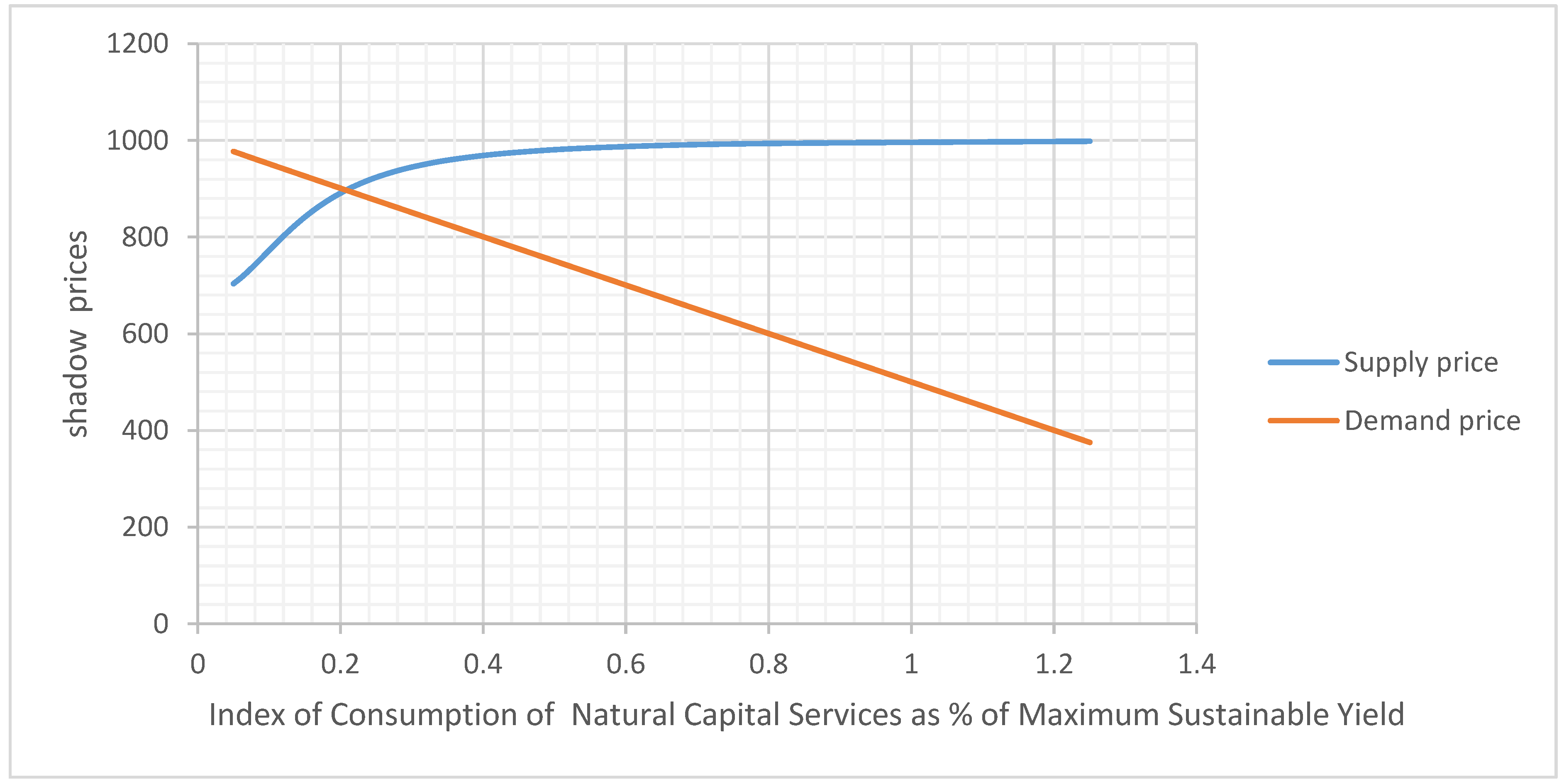
If the economy is not on an optimal path, therefore, we have two distinct sets of shadow prices, one from the opportunity costs (the difference between the rate of time preference and the marginal productivity of the two types of capital) on the supply side, given by equations (11) and (13), and one from the derived demand for capital and natural resources, given by equations (17) and (18). In general, we should expect these two sets of shadow prices to exhibit sharply different behaviors for increasing rates of ecosystem services use. Demand prices (marginal utilities) will tend to decline with consumption and ecosystem use. Marginal productivities will also tend to decline, implying that supply prices (social opportunity costs) will generally increase with the increase in the use of both types of capital. For any ecosystem service, before the intersection between the two price curves, the supply price will be below the demand price, meaning that the rate of exploitation of physical or natural capital can be increased with net social benefit (marginal benefit greater than social cost). The opposite will occur after the intersection between demand and supply. Along the optimum path, on the other hand (the intersection point), the two shadow prices are equal, while for a rate of usage greater than the optimum the two curves will diverge with larger and larger marginal net social costs.

Proposition 5. The optimal rate of growth is defined by the equality between marginal benefits and marginal costs.

Proof: Differentiating both sides of equation (17), and applying (11) we obtain:

p_{K}^{*} (ρ - Ω_{k} - R_{K}) = U_{C C}^{*} \dot{C} \to g^{*} = \frac{\dot{C}}{C} = \frac{1}{η} (Ω_{k} {+ R}_{K} - ρ)

(19)

where

g^{*}

indicates the optimal growth rate of consumption and can be recognized as a general form of the Ramsey- Koopman rate, while

η = - \frac{U_{C C}}{U_{C}} C

is the elasticity of the marginal utility of consumption. The optimal rate of growth will be uniquely defined by (20) if this elasticity does not change with the level of consumption, i.e. in the case of isoelastic utility. Note that the expression obtained holds both in the condition of perfect market equilibrium with no residuals

R_{K} = 0

, and in the case where market imperfections or externalities lead to market imbalances. In these cases,

R_{K} > 0

implies that a central planner, by taking into account the spillover effects ignored by the individual firms, could achieve a higher growth. Conversely,

R_{K} < 0

implies that growth will be lower than than the first best since market distortions increase the opportunity cost of foregoing consumption (the full rate of time preference

ρ

). In the case where this leads to unemployment (the Keynesian case), government policies that expand aggregate demand will increase the rate of growth to the extent that they counteract the negative effect

R_{K}

. Beyond such neutralizing effect, however, they will result in overheating the economy and repressed inflation.

Similarly, differentiating both sides of (18) and applying equation (12), we obtain:

[(ρ - S_{N} - μ (1 - 2 \frac{N}{N_{M}}) - \frac{U_{N}}{U_{Q}}] = - η \dot{\frac{C}{C}} - ϵ \frac{\dot{Q}}{Q}

(20)

{⟶ g}_{Q}^{*} = \frac{\dot{Q}}{Q} = \frac{1}{ε} [γ \frac{U_{N}}{U_{C} (F_{Q} - f_{Q)}} - (μ (2 \frac{N}{N_{M}} - 1) + S_{N}) - {(Ω}_{K} + R_{K}))]

where

g_{Q}^{*}

is the optimal rate of growth of ecoservice extraction and

ε = - \frac{F_{Q Q} - f_{Q Q}}{F_{Q} - f_{Q}} Q

is the elasticity of net marginal productivity of ecosystem services, as a measure of the severity of the decreasing returns to scale in ecoservice use.

Remarks. Note that the discount rate is not present in this result, since marginal costs from reduction of consumption growth are directly subtracted from marginal benefits from growth of ecoservice uses. In this case the optimal growth of ecoservice use is larger the larger its marginal benefits (the utility from non-consumptive use) and the smaller its marginal costs. These include both the marginal reduction in the stock of natural capital, the marginal increases in the effects of overextraction and the marginal productivity of physical capital net of its own marginal distortionary effects. Expression (20) thus indicates a direct trade-off between consumption of goods and indirect consumption of ecoservices. Moreover, because by definition in the steady state

\frac{\dot{C}}{C} =

\frac{\dot{Q}}{Q} = 0

, in the first best case of no market distortions (

R_{K} = S_{K} = 0)

, expressions (19) and (20) imply that:

\frac{U_{N}}{U_{C} (F_{Q} - f_{Q)}} + μ (1 - 2 \frac{N}{N_{M}}) = Ω_{K} = ϱ

. The (first best) steady state is thus an equilibrium condition where marginal benefits are equated to each other and to the opportunity cost of delaying consumption.

Proposition 6. Sustainable growth requires that marginal benefits and marginal costs converge over time. In turn this will require that the growth trajectory is below (above) the optimal Ramsey-Koopmans growth path.

Proof: Totally differentiating equation (17) we obtain as a condition for convergence:

U_{C C} \dot{C} - p_{k} (ρ + R_{K} - Ω_{K}) \dot{K} = - η U_{C} \frac{\dot{C}}{C} + p_{k} K (Ω_{K} - R_{K} - ρ) \frac{\dot{K}}{K} \leq 0

(21)

If the difference in (21) is negative, for any positive rate of growth, demand prices (marginal utilities) will tend to decrease over time, as growth implies larger and larger use of capital while supply prices will tend to increase. Consequently, the two prices will become closer and closer and will be equal to each other if (Ramsey-Koopmans) optimal growth is achieved. Conversely, if the difference in (21) is positive, the two prices will diverge. Solving (24) for the growth rate of consumption obtains:

\frac{\dot{C}}{C} \leq \frac{p_{k}}{U_{C}} \frac{(Ω_{K} - R_{K} - ρ)}{η}

(22)

This implies in turn that the condition for two prices to converge is that the ratio between marginal benefits and marginal costs is lower or equal to the ratio between the current and the optimum growth rate:

\frac{U_{C}}{p_{k}} \leq \frac{g^{*}}{g}, where g = \frac{\dot{C}}{C} is the current growth rate and g^{*} = \frac{(Ω_{K} - R_{K} - ρ)}{η}

(23)

For natural capital, assuming production function separability between consumption and ecosystem services, totally differentiating expression (12), and imposing convergence, we obtain:

\frac{\partial}{\partial t} (p_{n} - U_{c} \frac{(F_{Q} - f_{Q}}{γ}) = (ϱ - μ (1 - \frac{2 N}{N_{M}}) - S_{K}) p_{n} - U_{N} - U_{c c} \frac{(F_{Q} - f_{Q})}{γ} \dot{C} - U_{c} \frac{(F_{Q Q} - f_{Q Q})}{γ} \dot{Q} \leq 0

(24)

Simplifying and indicating the marginal utility of ecosystem services as:

U_{Q} = U_{c} \frac{(F_{Q} - f_{Q}}{γ}

, we find that the condition for convergence for the rate of growth of ecosystem service use depends on the growth rate of consumption:

\frac{\dot{Q}}{Q} \leq \frac{1}{ε} [\frac{U_{N}}{U_{Q}} + (μ (1 - \frac{2 N}{N_{M}}) + S_{N} - ρ) \frac{p_{N}}{U_{Q}} - η \frac{\dot{C}}{C}]

(25)

If consumption growth is optimal,

η \frac{\dot{C}}{C} = Ω_{K} + R_{K} - ρ

and, if both rates are optimal (

\frac{p_{N}}{U_{Q}} = 1

) , and for isoelastic utility

\frac{\dot{C}}{C} = \frac{1}{η} (Ω_{k} + R_{K} - ρ)

, we find again the expression for the optimal growth rate in (20).

Remarks

If the economy is not on an optimal path, we have two distinct sets of shadow prices, one from the opportunity cost or supply side, given by equations (11) and (12) and one from the derived demand for capital and natural resources, given by equations (15) and (16). Figure 1 shows how these two (demand and supply) sets of shadow prices behave for increasing rates of ecosystem services use. The demand price (net rents+ marginal contribution to the value function) tends to decline with ecosystem use, the marginal contribution becoming zero at the intersection (the optimum) and then becoming negative. The supply price (the social opportunity cost), on the other hand, tends to increase with the increase in the use of natural capital. Before the intersection between the two curves at the optimal rate (at the 20% of the maximum sustainable rate in the figure), the supply price is below the demand price, meaning that the rate of exploitation of natural capital can be increased with net social benefit (marginal benefit greater than social cost). Along the optimum path, on the other hand (the intersection point) the two shadow prices are equal, while for a rate of usage greater than 20% the two curves start diverging with larger and larger marginal net social costs.

The Steady State

In the steady state, the residual terms

R (K)

and

S (N)

accelerate the slow down and the reaching of stationarity of physical and natural capital if they are negative, while they act as delaying factors if they are positive, and their second derivatives are negative. However, if these derivatives are non-negative, endogenous growth emerges, proceeding at a constant rate in the case of zero second derivatives and becoming explosive when they are positive. If market distortions rather than positive externalities prevail, as in pure neoclassical model, steady state growth will be driven only by exogenous factors, such as population and technical progress, so that all other variables are stationary with zero-time derivatives. For shadow prices, this implies that the net marginal productivity of capital equals the rate of time preference. In the case of physical capital, whose marginal productivity decreases with growth, this implies a constant capital stock per unit of labor. For natural capital, the net marginal productivity also tends to decrease with the increase in the accumulation of natural capital and reaches zero once the size of stock N reaches one half of the maximum carrying capacity.

Proposition 7. In a steady state, the stock of physical capital equals the present value of consumption minus the present value of the ecosystem services.

Proof:

From equation (2), we derive, for

\dot{K} = 0

:

\frac{F (K, Q)}{K} - θ - \frac{C}{K} - \frac{f (K, Q)}{K} + \frac{R (K)}{K} = 0

(26)

and from equation (11):

F_{K} - θ - f_{k} + R_{K} - ρ = 0

(27)

Subtracting member by member equation (27) from equation (26), we obtain:

(\frac{F (K, Q)}{K} - f_{k}) - \frac{C}{K} - (\frac{f (K, Q)}{K} - f_{k} + (\frac{R (K)}{K} - R_{K}) + ρ = 0

(28)

Assuming that all functions are linear homogeneous:

F_{Q} \frac{Q}{K} - \frac{C}{K} + (F_{Q} - f_{Q}) \frac{Q}{K} + ρ = 0 \to K^{*} = \frac{C - (F_{Q} - f_{Q}) Q}{ρ}

(29)

Proposition 8. In a steady state, the stock of natural capital equals twice the present value of the rate of extraction at the social discount rate. This ensures sustainability provided that the ecosystem does not operate beyond its maximum regenerative capacity (

N_{M} = 2 N)

thereby preventing the depletion of natural capital. The social discount rate equals the rate of time preference plus the natural rate of regeneration plus the positive (or minus the negative) marginal value of ecosystem externalities minus the marginal non consumptive value of natural capital.

Proof:

From equation (3) we derive, for

\dot{N} = 0

:

μ (1 - \frac{N}{N_{M}}) - γ \frac{Q}{N} + \frac{S (N)}{N} = 0

(30)

And from equation (12) for

\dot{\frac{p_{N}}{p_{N}}} = 0

:

ρ - S_{N} - μ (1 - \frac{2 N}{N_{M}}) - \frac{U_{N}}{p_{N}} = 0

(31)

where the non-depletion condition that marginal reproduction rate

μ (1 - \frac{2 N}{N_{M}})

is nonnegative requires

N_{M} \geq 2 N .

Dividing (30) by N, and assuming linear homogeneity of

S (N)

, we obtain⁹:

μ - μ \frac{N}{N_{M}} - γ \frac{Q}{N} + S_{N} = 0

(32)

Solving equation (32) for

μ \frac{N}{N_{M}}

and substituting into equation (31), yields, for the steady state value of natural capital

N^{*}

:

N^{*} = \frac{2 γ Q}{μ + S_{N} + ρ - \frac{U_{N}}{p_{N}}}

(33)

Remarks

Equation (33) is yet another form of the Hamilton-Jacobi equation stating that the return to natural capital in the steady state should equal twice the value of the natural services extracted. This result includes a sustainability requirement of extraction rates depending on the condition

2 N \leq N_{M}

that ensures that natural capital is not higher than the natural reproduction level that maximizes capital formation according to the logistic equation. Note also that

p_{N}

is undefined in the general case, while it is equal to

\frac{U_{C} (F_{Q} - f_{Q})}{γ}

along the optimal path (see expressions (15) and (16)).

Proposition 9. In a steady state, when the ecosystem operates at maximum efficiency, the stock of natural capital equals the present value of the extraction rate. This condition ensures sustainability by balancing extraction with the ecosystem's maximum regenerative capacity. The social discount rate is the sum of the rate of time preference, half the natural regeneration rate minus the marginal non-consumptive value of natural capital.

Proof

Subtracting equation (31) from (32) and rearranging we obtain the following result:

N^{*} = \frac{N_{M}}{μ} (γ \frac{Q}{N} + \frac{U_{N}}{p_{N}} - ρ)

(34)

Assuming maximum regeneration conditions

N_{M} = 2 N^{*}

, substituting into (34) and solving for

N^{*} :

N^{*} (\frac{μ}{2} - \frac{U_{N}}{p_{N}} + ρ) = γ Q ⟶ N^{*} = \frac{γ Q}{(\frac{μ}{2} + ρ - \frac{U_{N}}{p_{N}})}

(35)

Remarks: The inclusion of

\frac{μ}{2}

in the social discount rate is directly justified by the condition that only half of the regeneration capacity is necessary to support a stock at half of the carrying capacity. This ensures that the ecosystem operates at its optimal regenerative efficiency, preventing both overexploitation and underutilization.

Conclusions

This paper has explored the concept of natural capital from the point of view of the current literature and through the application-extension of the growth model to both a neoclassical and a neo-Keynesian specification. Treating natural capital as a form of accumulating productive wealth similar to physical capital generates several insights on the question of sustainability and the way it can be incorporated in economic evaluation through the use of shadow prices. The analysis developed has shown that shadow prices can be defined and estimated without explicit reference to supply-side endogenous optimization or to an optimal trajectory, as marginal costs directly emerge from the tradeoffs created by growth. These tradeoffs involve the consumption foregone to finance capital accumulation, conservation and maintenance of natural capital and any gap between demand and supply caused by market distortions and/or shortfalls of aggregate demand. They also reflect the complex relation between the two forms of capital, which are complementary within a range of moderate usage and appropriate maintenance of natural resources but become competitors outside this range. Two different conditions of sustainability emerging from this analysis are: (1) that social wellbeing and, at the same time the sum of net physical and natural capital changes are nondecreasing; (2) that marginal benefits and marginal costs from exploiting natural capital converge over time.

In the steady state, the economy achieves equilibrium with a stock of capital equaling the present value of consumption minus the present value of ecosystem services, with the social discount rate equal to the effective rate of time preference. In a second-best world, steady state equilibrium is not necessarily characterized by equality between aggregate supply and aggregate demand, even though the growth rates of consumption and capital per capita are zero. This means that there may be unemployment, waste as well as negative and positive externalities, which may persist in spite of the fact that the marginal productivity of capital has fallen below its opportunity cost. Consequently, the growth experienced by the economy to achieve a steady state will be lower and may be halted prematurely if market distortions and negative externalities prevail. On the other hand, growth may be higher and may even steady state sustained if positive externalities (such as those leading to endogenous technical change) prevail. Further aggregate growth can still occur due to exogenous factors such as population growth or productivity improvements.

For natural capital, necessary sustainable steady-state conditions imply that natural regeneration matches extraction. This requires a steady state stock of natural capital equaling twice the present value of the rate of extraction. The social discount rate in this case is different from the case of physical capital and includes both the rate of regeneration and marginal non consumptive utility. The steady-state stock of natural capital is thus such that it balances extraction rates with natural regeneration and economic valuation parameters. Moreover, a sufficient condition for sustainability is ensuring that the ecosystem operates at maximum efficiency (natural capital equal to ½ of maximum sustainable level:

N^{*} = \frac{N_{M}}{2}

) .

Notes

1	https://data.worldbank.org/data-catalog/wealth-accounting. See also World Bank (2006), (2011) and (2018).
2	https://digitallibrary.un.org/record/784798?ln=en
3	The deviation from the optimal capital-labor ratio can be linked directly to wage rigidities. Suppose $w > w^{}$ , the equilibrium wage. Then the actual employment is L_d <L_e the full-employment labor force. Hence, the actual capital-labor ratio K_e is higher than the full employment ratioK^ both because labor is lower and because capital is higher due to the substitution effect. A higher capital labor ratio implies that the additional capital per worker is not optimally matched by labor to make it productive and may result in some capital being less productive or lying idle. For any given level of the elasticity of substitution between capital and labor, the larger the discrepancy between the current and the full employment capital labor ratio, the higher the value of R(K(t).
4	For other natural renewable resources, the logistic function is still appropriate but requires suitable modifications. In the case of water, for example, renewable water resources, such as groundwater or surface water in a watershed, can fit into this framework. In this case, $μ$ could represent the natural recharge rate, such as replenishment by rainfall or aquifers, while N_M may represent the maximum sustainable water level in an aquifer or reservoir. In the case of nonrenewable resources μ = 0 and the equation would be dominated by the extraction term γQ(t) with γ ≥ 1.
5	For “time autonomy”, it is meant that the utility function does not depend directly on time, but only indirectly through its arguments.
6	The Hamilton-Jacobi equation describes the evolution of the value function in a dynamic system. It connects the present value of the system's state to the instantaneous utility (or cost) and the dynamics of the system.
7	The general argument advanced by Keynes for the shortfall of aggregate demand is more appropriately captured by a growth model because it was not one of persistent market distortions in the static sense, but rather of a sort of dynamic failure to adjust. This failure was aggravated by the fact that “…an outstanding characteristic of the economic system in which we live [is that] whilst it is subject to severe fluctuations in respect of output and employment, it is not violently unstable. Indeed, it seems capable of remaining in a chronic condition of sub-normal activity for a considerable period without any marked tendency either towards recovery or towards complete collapse” (Keynes, 1936, p. 249).
8	As explained by Hoover (1995), in the Keynesian system, not only wage rigidities, but also concern for relative wages can force the economy into a stable configuration below full employment.
9	This depends on equation (31) implying: $μ \frac{N}{N_{M}} = \frac{1}{2} (μ + S_{N} + \frac{U_{N}}{p_{N}} - ρ) .$ Substituting into (30) and assuming linear homogeneity of S(N), yields: $\frac{1}{2} (μ + S_{N} + \frac{U_{N}}{p_{N}} - ρ) = μ - γ \frac{Q}{N} + S_{N}$ . Solving for $γ Q = \frac{1}{2} (μ + S_{N} + ρ - \frac{U_{N}}{p_{N}}) N$ . This is a steady state condition but also an upper bound to a sustainable one, since N ≤ 2N_M to avoid depletion.

References

Barbier, Edward B. 2011. Capitalizing on nature. New York: Cambridge University Press.
Cohen, A. (2010). Capital controversy from Bhohm-Bawerk to bliss: badly posed or very deep questions? Or what We can learn from capital controversy even if you Don’t care who won. Journal of the History of Economic Thought, 32(1), 1–21.
Coase, R. H. (1960), "The Problem of Social Cost", 3 Journal of Law and Economics, 1-44.
Eisner, Robert [1988] "Extended Accounts for National Income and Product", Journal of Economic Literature, 26, December, pp. 1611-1684.
El-Serafy, S. [ 1981] "Absorptive Capacity, The Demand for Revenue, and the Supply of Petroleum", Journal of Energy and Development, 7, No. 1, Autumn.
Fenichel E.P. and Abbot, J.K. (2014), Natural Capital: From Metaphor to Measurement, Journal of the Association of Environmental and Resource Economists 2014 1:1/2, 1-27.
Anne D. Guerry, Stephen Polasky, Jane Lubchenco, Rebecca Chaplin-Kramer, Gretchen C. Daily, Robert Griffin, Mary Ruckelshaus, Ian J. Bateman, Anantha Duraiappah, Thomas Elmqvist, Marcus W. Feldman, Carl Folke, Jon Hoekstra, Peter M. Kareiva, Bonnie L. Keeler, Shuzhuo Li, Emily McKenzie, Zhiyun Ouyang, Belinda Reyers, Taylor H. Ricketts, Johan Rockström, Heather Tallis, Bhaskar Vira, (2018) “Natural capital informing decisions”, Proceedings of the National Academy of Sciences Jun 2015, 112 (24) 7348-7355. [CrossRef]
Hart, O. (1995), "Corporate Governance: Some Theory and Implications", 105(430) Economic-Journal, 678-89. [CrossRef]
Hartwick, J.M., 1990. Natural resources, national accounting and economic depreciation. Journal of public Economics, 43(3), pp.291-304. [CrossRef]
Kirzner, I. M. (1996). Ludwig von Mises and the theory of capital and interest. In I. M. Kirzner (Ed.), Essays on capital and interest (pp. 123–133). Brookfield: Eward Elgar.
Lewin, P. ([1999] 2011). Capital in Disequilibrium: The Role of Capital in a Changing World. Auburn: Ludwig von Mises Institute (first edition, London: Rouledge).
Lucas Jr, R.E., 1988. On the mechanics of economic development. Journal of monetary economics, 22(1), pp.3-42.
Medema, S. and Samuels, W.J. (1996), Foundations of research in economics: How do economists do economics, Advances in Economic Methodology series, Cheltenham, U.K. and Lyme, N.H.: Elgar; distributed by American International Distribution Corporation, Williston, Vt., 298.
Lewin, P. and Cachanosky, N. (2018), Value and capital: Austrian capital theory, retrospect and Prospect. Rev Austrian Econ (2018) 31: 1. [CrossRef]
Romer, P.M., 1990. Endogenous technological change. Journal of political Economy, 98(5, Part 2), pp.S71-S102.
Samuels, W.J. (1974) "Commentary: An Economic Perspective of the Compensation Problem", 21, Wayne Law Review, 113-34.
WORLD BANK (2006), Where is the Wealth of Nations?. The International Bank for Reconstruction and Development/The World Bank, Washington D.C.
World Bank (2011), The Changing Wealth of Nations. Measuring Sustainable Development in the New Millennium. The International Bank for Reconstruction and Development/The World Bank, Washington D.C.
World Bank (2018), Glenn-Marie Lange Quentin and Wodon Kevin Carey (Editors ) The Changing Wealth of Nations. Building a sustainable Future. The International Bank for Reconstruction and Development/The World Bank, Washington D.C.
Samuelson, P.A., 1981. Bergsonian welfare economics. Economic welfare and the economics of Soviet socialism: essays in honor of Abram Bergson, pp.223-66.
Solow, R.M., 1986. On the intergenerational allocation of natural resources. The Scandinavian Journal of Economics, pp.141-149. [CrossRef]
Weitzman, M.L., 1976. On the welfare significance of national product in a dynamic economy. The quarterly journal of economics, 90(1), pp.156-162. [CrossRef]
Ward, M., 1982 Accounting for the Depletion of Natural Resources in the National Accounts of Developing Countries", OECD Development Center, 1982.

Figure 1.

Disclaimer/Publisher’s Note: The statements, opinions and data contained in all publications are solely those of the individual author(s) and contributor(s) and not of MDPI and/or the editor(s). MDPI and/or the editor(s) disclaim responsibility for any injury to people or property resulting from any ideas, methods, instructions or products referred to in the content.

© 2025 by the authors. Licensee MDPI, Basel, Switzerland. This article is an open access article distributed under the terms and conditions of the Creative Commons Attribution (CC BY) license (http://creativecommons.org/licenses/by/4.0/).

Copyright: This open access article is published under a Creative Commons CC BY 4.0 license, which permit the free download, distribution, and reuse, provided that the author and preprint are cited in any reuse.

Natural Capital: The Quest for Sustainability

Abstract

Keywords:

Subject:

Introduction

The Theoretical Framework

The Concept of Capital

The Underlying Economic Model and the Role of Shadow Prices

Conclusions

Notes

References

MDPI Initiatives

Important Links

Subscribe