Empirical Time Complexity for Assessing the Algorithm Computational Consumption on a Hardware

Yue Wu; Carlo Vittorio Cannistraci

doi:10.20944/preprints202501.2185.v1

Submitted:

28 January 2025

Posted:

29 January 2025

You are already at the latest version

Abstract

Scalability is an important aspect of algorithm design. Typical methods for accessing scalability in terms of running time include theoretical time complexity by algorithm analysis, and model-fitting time complexity derived from simulation results. However, theoretical time complexity often fails to account for real-world conditions in algorithm implementation such as influence from compilers, and lacks a simulation-based examination method. Alternatively, model-fitting time complexity is prone to learn a model with incorrect scaling orders. Here, we propose the empirical time complexity (ETC), which is a data-driven model-free and parameter-free method to account for the factors influencing an algorithm; for instance, the crosstalk between algorithm realization, compilation and hardware implementation. This can be used to guide code optimization and to gain algorithmic maximum efficiency for specific hardware, programming language or compiler. The values of ETC in function of an input variable form a curve that offers a visual representation of how an algorithm scale with input size. When the ETC curves of different versions of an algorithm are reported together with the theoretical time complexity curve, their comparison allows to select what versions are closer to the theoretical complexity. To showcase the utility of ETC in real scenarios, we investigated two sets of algorithms (graph shortest path and matrix multiplication) and we offer evidence on how ETC is crucial for diagnostic and optimized design of algorithms as close as possible to their theoretical limit.

Keywords:

Time complexity

;

Algorithm scalability

;

Empirical complexity

;

Big data

;

Machine learning

Subject:

Computer Science and Mathematics - Data Structures, Algorithms and Complexity

Introduction

Data mining and machine learning have been widely applied to solve problems in various fields and demonstrate outstanding capability [1]. However, they usually require a large amount of data to work effectively, which combined with factors including dealing with big data [2], hyperparameters tuning [3], and data augmentation [4], constituting a notable problem that causes slowdown of algorithms, and such slowdown cannot be cost-efficiently solved by simply piling up computation resources (Figure 1a). Developing more scalable algorithms is a viable solution, for which the time complexity is usually used to assess the scalability.

Time complexity can be divided into theoretical time complexity (TTC) and model-based time complexity (MBTC). TTC usually involves giving complicated analysis to derive rigorous upper, lower, or asymptotic bounds [5,6], requires open source code, and cannot serve as an examination method for a real computer. As the counterpart, MBTC has been revealed to overcome these disadvantages, which focuses on typical cases and eliminates the need for finding complexity bounds [7]. A bootstrap re-sampling-based approach [8] and a subsequent automatic analyzer – empirical scaling analyzer (ESA) [9] were developed, enabling internal statistical examinations of fitted models for more convincible complexity estimation, and the applications of ESA were investigated in evaluating solvers for problems such as travelling salesman problem [10,11,12]. However, these types of model-based time complexity still necessitate modelling and a fitting algorithm to determine the order and coefficients of the model, and the time fluctuation from different running instances leads to different scaling orders.

Pegny [13] pointed out that some of the hypotheses in the computational complexity theory (CCT), on which TTC is based, does not reflect real-world computing machines (Figure 1c). First, CCT assumes hardware-independence, while the algorithm complexity, or scalability, in real-world computers are sensitive to hardware details. Second, CCT assumes computation model-independence, but when computing machines realized by different principles started to be used in practice, each type has its own complexity classes and CCT cannot unify them. Third, in the Extended Church Turing thesis (ECTT), the term “reasonable” was not well-defined, thus leaving space for treating time complexity from an empirical point of view.

In this study, along the empirical point of view, we propose the empirical time complexity (ETC), as a new hardware-aware complexity assessing approach different from TTC and MBTC. ETC measures how the time consumption of an algorithm scales with increasing input size, providing a quantification for algorithmic scalability. Experiments were performed to validate the characteristics of ETC, in which one simulation on graph shortest path algorithms shows that ETC aligns in general with the theoretical time complexity when there is little crosstalk, while another simulation on different matrix multiplication algorithms shows that the discrepancy part between ETC and the theoretical time complexity reveals hardware/compiler/algorithm crosstalk in algorithm implementations. The ability of ETC to identify crosstalk can in turn guide code optimization for developers. Moreover, ETC offers a visualization for algorithm scalability and makes it possible for the scalability of different algorithms compared in a single figure.

Results

ETC as a Visualization of Approximated TTC

In network science, computing shortest path between any two nodes in a graph is an important question, and faster, large-scale algorithms have been studied all the time, making it a pertinent example to our study. 3 algorithms in Matlab were tested, among which two are Matlab toolbox function graphshortestpath [14], implemented with breadth-first search (BFS) and Dijkstra’s algorithm in mex code, which have time complexity of

O (N + E)

and

O (E l o g N)

, where

N

and

E

are the number of nodes and links respectively; the other is the native Dijkstra’s algorithm [15] with mat file, which has

O (N^{2})

theoretical complexity.

Unweighted and undirected networks were generated using the nPSO model [16], which is an algorithm for generating real-world-like networks. The half average node degree was set approximately to 50 such that

E = k N

where

k

is a constant irrelevant to

N

. With such setting, the theoretical time complexity of graphshortestpath became

O (N)

for BFS and

O (N l o g N)

for Dijkstra’s algorithm, and the native Dijkstra’s algorithm remained its time complexity

O (N^{2})

. The algorithms were tested in single-core computing mode on networks with the size from 1,000 nodes to 32,000 nodes, and were repeated for 6 times from which the first repetition was dropped for stability.

The ETC and running time are shown in Figure 2a and 2b, which show that the ETC curve of the native Dijkstra algorithm almost overlaps with the TTC

O (N^{2})

. For the other two algorithms, the ETC curves largely capture the TTC, and the order of ETC between the two algorithms reflected the true order of their TTC. The potential reason for the disturbance on the ETC curve from the ideal ones is that since these two algorithms are based on Matlab toolbox, there may exist some code for software integration in algorithm realization but not essential as core algorithms, which can be viewed as algorithm realization level crosstalk.

ETC Reveals Practical Scalability Influenced by Crosstalk

In theory, TTC should predict the running time for certain input size based on available running time results on smaller input data size, but this is not always the case since the following factors are missing in TTC. First, modern computers have complex architectures such as optimized memory architecture in which there are different levels of CPU cache as well as registers, to support efficient computation, which usually have increasing size for higher layer caches. This architecture causes nonlinear computation resource utilization with regard to data size, thus nonlinear running time. Second, different programming languages and compilers produce different machine code, which also contribute to nonlinear running time behavior.

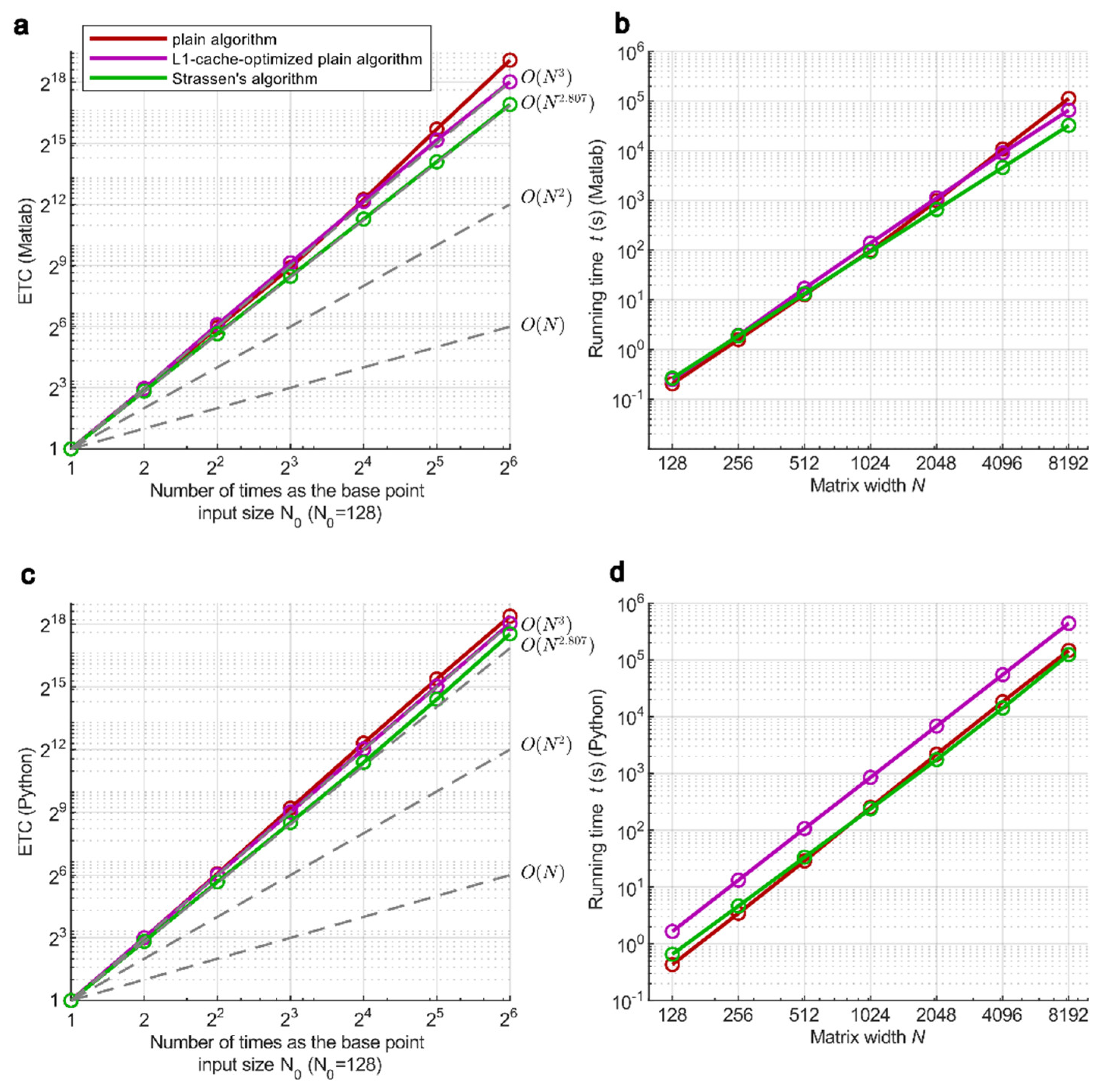
To test how ETC behaves under such conditions, the experiments on matrix multiplication were performed, including plain matrix multiplication (

O (N^{3})

time), Strassen’s algorithm [17] (

O (N^{2.807})

time), and a modified plain multiplication with L1-cache optimized algorithm [18] (

O (N^{3})

time). These algorithms were tested in single-core computing mode in both Matlab and Python, with the ETC (Figure 3 a and c) and practical running time (Figure 3 b and d) shown. The results show that the ETC of these algorithms in general matches their declared theoretical time complexity.

As an improved algorithm, the plain algorithm is optimized by decomposing the matrix into small blocks on which the plain matrix multiplication is performed. This method optimized data transfer between caches by preventing excessive data transfers outside CPU L1-cache, leading to a better efficiency. Consequently, ETC of the optimized plain algorithm is shown to follow closely to the TTC in Figure 3 (a) and (c). In contrast, the plain algorithm subjects to a nonlinear behavior when input size exceeds certain threshold, due to sudden excessive data transfer between L1- and L2-caches which is slower, and this increase of data transfer is not linear to the change of input size. The comparison between the plain algorithm and the L1-cache optimized algorithm indicates that ETC is able to reflect hardware crosstalk in algorithm implementations. The figure also shows that Strassen’s algorithm in Python went beyond

O (N^{2.807})

(Figure 3c), while in Matlab it follows the TTC reference curve (Figure 3a), even if the same algorithm is used. This result indicates that there potentially exists compiler-level crosstalk, or a combination of factors from compiler and hardware crosstalk in Python implementation.

Mathematical Proof for ETC as a Complexity Measure

In this part we elaborate the necessity of normalizing the scaling variable, and the necessary condition to apply ETC to measure the complexity of an algorithm. We discuss the following cases of complexity models:

(a) Linear case: The complexity model can be written as

y = a x + b

. When

b \to 0

, define the dependent variable

\tilde{y} = \frac{a x}{a x_{0}} .

When the dependent variable is normalized by

x_{0} = 1

, it can be derived that

\tilde{y} = x

(i.e.,

l o g \tilde{y} = l o g x

). If a non-zero bias term exists, then

\tilde{y} = \frac{a x + b}{a x_{0} + b} = \frac{a}{a + b} x + \frac{b}{a + b}

, which drawn in linear space decreases the slope of the curve but adds a y-axis intercept, and in such scenario

l o g \tilde{y}

does not have a linear relation to

l o g x

.

(b) Quadratic case: The complexity model can be written as

y = a x^{2} + b x + c

. When

b, c \to 0

, define the dependent variable

\tilde{y} = \frac{a x^{2}}{a x_{0}^{2}} .

When the dependent variable is normalized by

x_{0} = 1

, it can be derived that

\tilde{y} = x^{2}

(i.e.,

l o g \tilde{y} = 2 l o g x

). When

b, c \neq 0

,

\tilde{y} = \frac{a x^{2} + b x + c}{a x_{0}^{2} + b x_{0} + c} = \frac{a}{a + b + c} x^{2} + \frac{b}{a + b + c} x + \frac{c}{a + b + c}

, for which

l o g \tilde{y}

can not be linearly expressed by

l o g x

.

(c) Arbitrary case: The complexity model can be written as

y = a_{n} x^{n} + a_{n - 1} x^{n - 1} + \dots + a_{1} x + a_{0}

. When

a_{i} \to 0 (i \neq n)

, define the dependent variable

\tilde{y} = \frac{a_{n} x^{n}}{a_{n} x_{0}^{n}} .

When the dependent variable is normalized by

x_{0} = 1

, it can be derived that

\tilde{y} = x^{n}

(i.e.,

l o g \tilde{y} = n l o g x

). A similar conclusion to the linear and quadratic case can be derived for the coefficients and bias term.

According to the above, the necessary condition to apply ETC is that the scaling variable approaches zero when the time approaches zeros, which means that the bias term in the complexity model should be zero. Thus, those parameters that does not approach the zero point do not satisfy the condition and should be excluded from the set of scaling variables.

Discussion

Modern computers have complex hardware architectures, and it is difficult or even impossible for developers to learn all the hardware details in order to optimize their code. For instance, memories are categorized into registers, L1, L2, L3 caches and main memory ordered by distance to the processors and by data transfer speed in reverse. If GPU is involved, there is also data transfer between CPU and GPU. These factors act together leading to complex behavior of running time with regard to input data size, therefore, TTC is not able to reflect the practical condition for algorithm implementation. In such case, ETC offers a method to examine how algorithms scale for specific computing machines on which the algorithms are implemented.

Additionally, there are different domains of computing, including classical computing (CPU and GPU), neuromorphic computing, quantum computing, and etc. Each domain has its specific TTC and complexity classes for algorithms with the same principle. Since ETC directly evaluates the absolute running time and derives the proportion, it does not change its intrinsic form for specific physical realization, serving as a one-for-all index for algorithm scalability. Therefore, ETC has the potential to be a generic index that can be used to compare practical scalability for all general algorithms across computation domains.

From the generalized perspective, ETC is highlighted by two features: 1) In the cross-domain or hybrid-domain settings, ETC can be used to directly compare practical scalability of general algorithms, which considers the presence of crosstalk resulted from various forms of heterogeneity during algorithm implementation. 2) In the within-domain (pure) setting, ETC is able to approach the TTC of its own domain in the presence of little crosstalk, and if these two do not match, ETC can discover the crosstalk and assist to optimize the way to implement the algorithm by reducing this gap, such that the computation approaches the pure-domain TTC.

Lastly, as analyzed in the proof, the bias in the complexity model also affects the interpretation of ETC. For instance, an algorithm might have a large running time for the base point and a low ETC. This usually indicates that the algorithm is not realized in an appropriate way such that the overhead is too significant, or to the extremity the algorithm is not very practical to be used such as those galactic algorithms in matrix multiplication. However, ETC offers an approach to optimize the algorithm with respect to both ETC and the overhead time individually, providing more convenience for code optimization.

In conclusion, this study suggests a new method ETC for evaluating algorithmic scalability, which is able to show how the time consumption of algorithms scales with increasing input size. Compared to MBTC, ETC avoids the possibility of fitting inappropriate scaling orders, and compared to TTC, it is free from complex analysis, and can serve as an experiment-based examination technique to validate TTC, thus reflecting the algorithm scalability with regard to input size, e.g., how large is practical to a dataset for algorithms to run on a particular hardware machine. Moreover, ETC is able to discover crosstalk among code implementation, hardware and compiler. Thus, ETC can assist developing efficient algorithms with regard to certain hardware and compiler. Whether a code is properly optimized can be examined by validating the extent to which ETC is close to theoretical curves.

Materials and Methods

Empirical Time Complexity (ETC)

To obtain ETC, first a series of running times is collected by running the algorithm using data with increasing input sizes, after which a normalization step is performed by dividing these running times by the running time of the smallest data size (base point). The running times and the ETC curves are plotted in two panels side by side to offer a visualization for overall scalability and speed of the algorithm. The axes are transformed to log-scale to direct reflect the scaling order of the algorithm. By comparing with a few ideal reference lines with different TTC, ETC reveals the scaling order of a tested algorithm. In the case where multiple repetitions are made for the same input size, normalization is performed for the running time sequence of each repetition and then ETC is reported with mean and standard deviation.

In mathematic formulation, given a series of

n

running times of an algorithm

t_{i}, i \in {0,1, 2, \dots, n - 1}

with increasing input sizes

N_{i}

, the ETC is defined as the proportion of the running time of each input size to the running time of the base point

{E T C}_{i} = t_{i} / t_{0}

, where

t_{0}

is the running time of the base point, which contains the overhead information and should be also taken into consideration when assessing the speed of an algorithm. ETC curve describes an overall scalability pattern for the algorithm. In the scenario of multiple input data dimensions, ETC is still applicable if linear relations can be established for each parameter with a unique parameter

N

.

Counting Running Time of Algorithms

For graph shortest path algorithm, ‘tic toc’ was used to count running time. For matrix multiplication, ‘profiler’ was used instead of ‘tic toc’ in both Matlab and Python to count running time, since this operation is done at the most bottom-level and the profiler can prevent compilers from automatically optimizing code such that it is implemented as close to the tested algorithm as possible. The profiler approach would lower down the algorithm implementation speed, but this does not constitute a problem, since our goal is to assess the scalability, rather than benchmarking absolute running time.

For the graph shortest path function of Matlab toolbox, since the toolbox functions are fast (lower complexity than matrix multiplication) such that a baseline time the profiler introduces contributes a large part of the time consumption, we turned to used ‘tic toc’ to count time for the graph shortest path functions.

Matrix Multiplication

In the case of matrix multiplication, a L1-cache-optimized algorithm was implemented to show how code implementation is influenced by hardware architecture. The algorithm loops over submatrices of 8x8 size which can be fit entirely into L1-cache of modern CPU (typical size is 512K) and are efficiently computed there since less data transfer is required from and to higher layers involved which has a higher latency. With this optimization, the number of data transfer from and to L1-cache changes continuously with the square matrix width, thus, the algorithm should achieve scalability ETC close to the TTC with regard to square matrix width.

Hardware and Software Specifications

All simulations were performed on Lenovo P620 workstation, equipped with AMD Ryzen Threadripper PRO 3995WX 2.7GHz CPU that has 64 cores and 128 threads. GPU was not used in the simulations. Ubuntu 20.04, MATLAB 2021b, Python 3.11.7, VS code 1.86.2 were used as the environments to run the algorithms. Matlab was opened in single thread computation mode; Matlab and VS code were given the highest priority in the operating system.

Author Contributions

C.V.C. proposed ETC and designed the experiments and the content of the study. Y.W. performed the experiments and collected the results. C.V.C and Y.W. analyzed the experiment results. C.V.C. designed and Y.W. realized the figures. Y.W. wrote the manuscript and C.V.C. corrected it.

Funding

This work is supported by the Zhou Yahui Chair professorship of Tsinghua University, the starting funding of the Tsinghua Laboratory of Brain and Intelligence, and the National High-level Talent Program of the Ministry of Science and Technology of China.

Data Availability Statement

The code to get results and produce figures in this study can be accessed from GitHub link: https://github.com/biomedical-cybernetics/Empirical-Time-Complexity

Acknowledgement

We thank: Junda Chen for the valuable scientific discussion. Yuchi Liu, Ruochen Xu, Wenli Zhu, Lixia Huang, and Weijie Guan for the administrative support at THBI.

Conflicts of Interest

The authors declare no competing interests.

References

Xu, Y.; Liu, X.; Cao, X.; Huang, C.; Liu, E.; Qian, S.; Liu, X.; Wu, Y.; Dong, F.; Qiu, C.-W.; et al. Artificial intelligence: A powerful paradigm for scientific research. Innov. 2021, 2, 100179. [Google Scholar] [CrossRef] [PubMed]
Qiu, J.; Wu, Q.; Ding, G.; Xu, Y.; Feng, S. A survey of machine learning for big data processing. EURASIP J. Adv. Signal Process. 2016, 2016, 67. [Google Scholar] [CrossRef]
Wu, J.; Chen, S.; Liu, X. Efficient hyperparameter optimization through model-based reinforcement learning. Neurocomputing 2020, 409, 381–393. [Google Scholar] [CrossRef]
Zhu, J. , Chen, N., Perkins, H. & Zhang, B. Gibbs max-margin topic models with data augmentation. Journal of Machine Learning Research 15, (2014).
Arora, S. & Barak, B. Computational Complexity: A Modern Approach. Complexity 1, (2007).
Cook, S.A. An overview of computational complexity. Commun. ACM 1983, 26, 400–408. [Google Scholar] [CrossRef]
Hooker, J.N. Needed: An Empirical Science of Algorithms. Oper. Res. 1994, 42, 201–212. [Google Scholar] [CrossRef]
Holger, H. Hoos. A Bootstrap Approach to Analysing the Scaling of Empirical Run-Time Data with Problem Size. (2009).
Pushak, Y.; Mu, Z.; Hoos, H.H. Empirical scaling analyzer: An automated system for empirical analysis of performance scaling. AI Commun. 2020, 33, 93–111. [Google Scholar] [CrossRef]
Mu, Z.; Dubois-Lacoste, J.; Hoos, H.H.; Stützle, T. On the empirical scaling of running time for finding optimal solutions to the TSP. J. Heuristics 2018, 24, 879–898. [Google Scholar] [CrossRef]
Hoos, H.H.; Stützle, T. On the empirical scaling of run-time for finding optimal solutions to the travelling salesman problem. Eur. J. Oper. Res. 2014, 238, 87–94. [Google Scholar] [CrossRef]
Mu, Z. Analysing the empirical time complexity of high-performance algorithms for SAT and TSP. (2015) . [CrossRef]
Maël Pégny. Computational Complexity: An Empirical View. (2017).
Mathworks. Graphshortestpath.
Jorge Barrera. Dijkstra very simple. Preprint at ( 2024.
Muscoloni, A.; Cannistraci, C.V. A nonuniform popularity-similarity optimization (nPSO) model to efficiently generate realistic complex networks with communities. New J. Phys. 2018, 20, 052002. [Google Scholar] [CrossRef]
Strassen, V. Gaussian elimination is not optimal. Numer. Math. 1969, 13, 354–356. [Google Scholar] [CrossRef]
Gunnels, J. A. , Henry, G. M. & van de Geijn, R. A. A family of high-performance matrix multiplication algorithms. in Lecture Notes in Computer Science (including subseries Lecture Notes in Artificial Intelligence and Lecture Notes in Bioinformatics) vol. 2073 (2001).

Figure 1. Algorithm scalability assessment and different types of time complexity. (a) Time complexity is the index to evaluate algorithm scalability that is critical to speed up algorithms in data mining and machine learning under the challenges from big data, hyperparameters tuning and data augmentation. (b) Comparison of advantages and limitations between TTC, MBTC and ETC. (c) The hypotheses in CCT is not complied with real-world computers with respect to its hardware-independence, model-independence and ECTT implies the use of an empirical point of view. (d) The features of ETC include hardware independence, being an experiment-based examination method, and offering a direct visualization for scalability. TTC: Theoretical time complexity; MBTC: Model-based time complexity; ETC: Empirical time complexity; CCT: Computational complexity theory; ECTT: Extended Church Turing thesis.

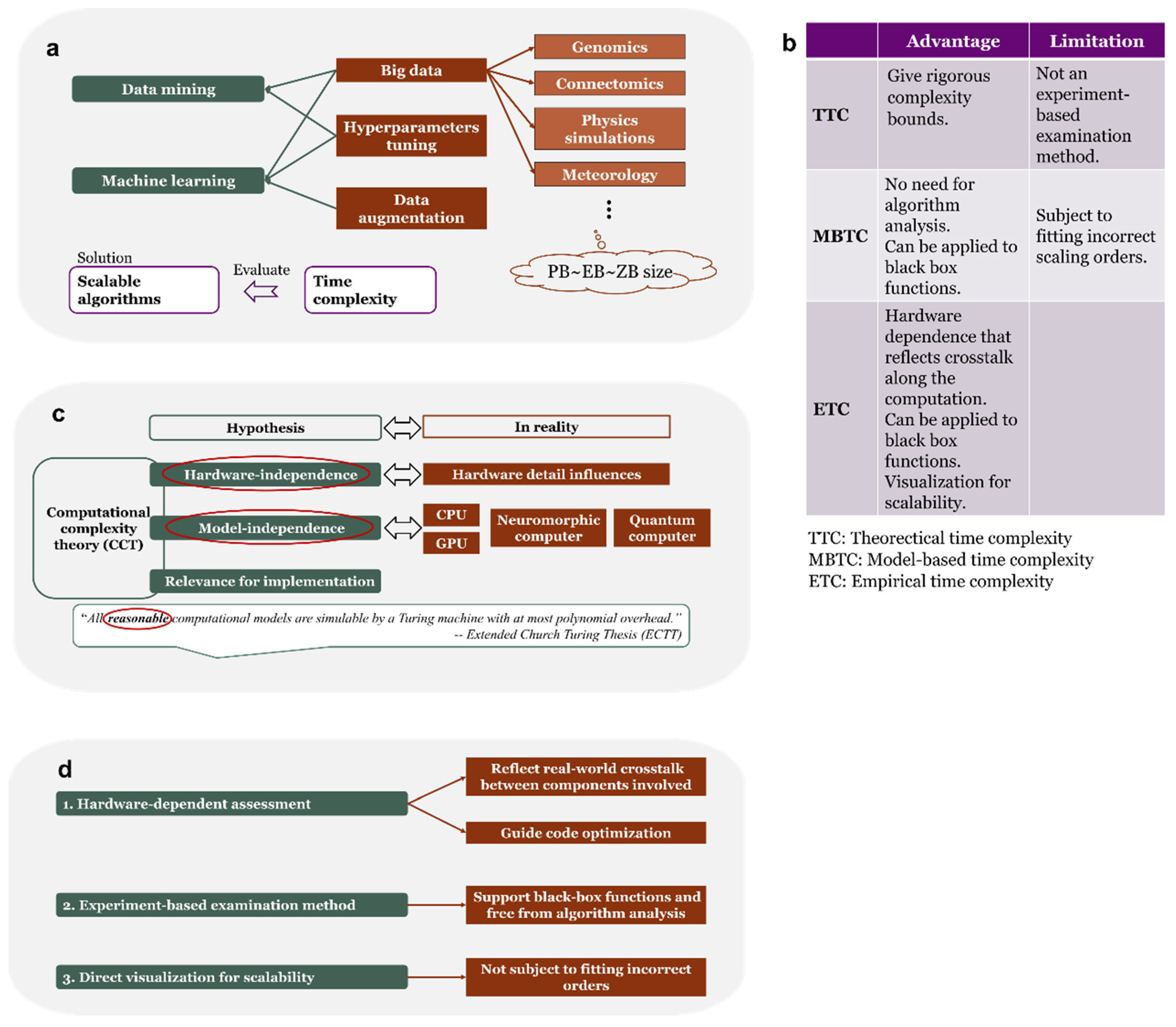
Figure 2. Empirical time complexity (ETC) and the running time of 3 shortest-path finding algorithms in Matlab. Different sizes of networks with

N

nodes and

E

links were generated by nPSO model to test algorithm speed. ETC in (a) was obtained by a normalization which divides the running time sequence in (b) by the running time of the smallest input data size. The simulations were repeated for 6 times with the first repetition removed for stability, and normalization in ETC was performed repetition-wise. The mean of tested points (circle mark) and standard deviation (in shade) are shown. The gray dash lines in (a) are the ETC references of ideal complexity models with cubic, square,

N l o g N

and linear time complexity. BFS: Bread-first search; nPSO: Nonuniform popularity-similarity optimization.

Figure 2. Empirical time complexity (ETC) and the running time of 3 shortest-path finding algorithms in Matlab. Different sizes of networks with

N

nodes and

E

links were generated by nPSO model to test algorithm speed. ETC in (a) was obtained by a normalization which divides the running time sequence in (b) by the running time of the smallest input data size. The simulations were repeated for 6 times with the first repetition removed for stability, and normalization in ETC was performed repetition-wise. The mean of tested points (circle mark) and standard deviation (in shade) are shown. The gray dash lines in (a) are the ETC references of ideal complexity models with cubic, square,

N l o g N

and linear time complexity. BFS: Bread-first search; nPSO: Nonuniform popularity-similarity optimization.

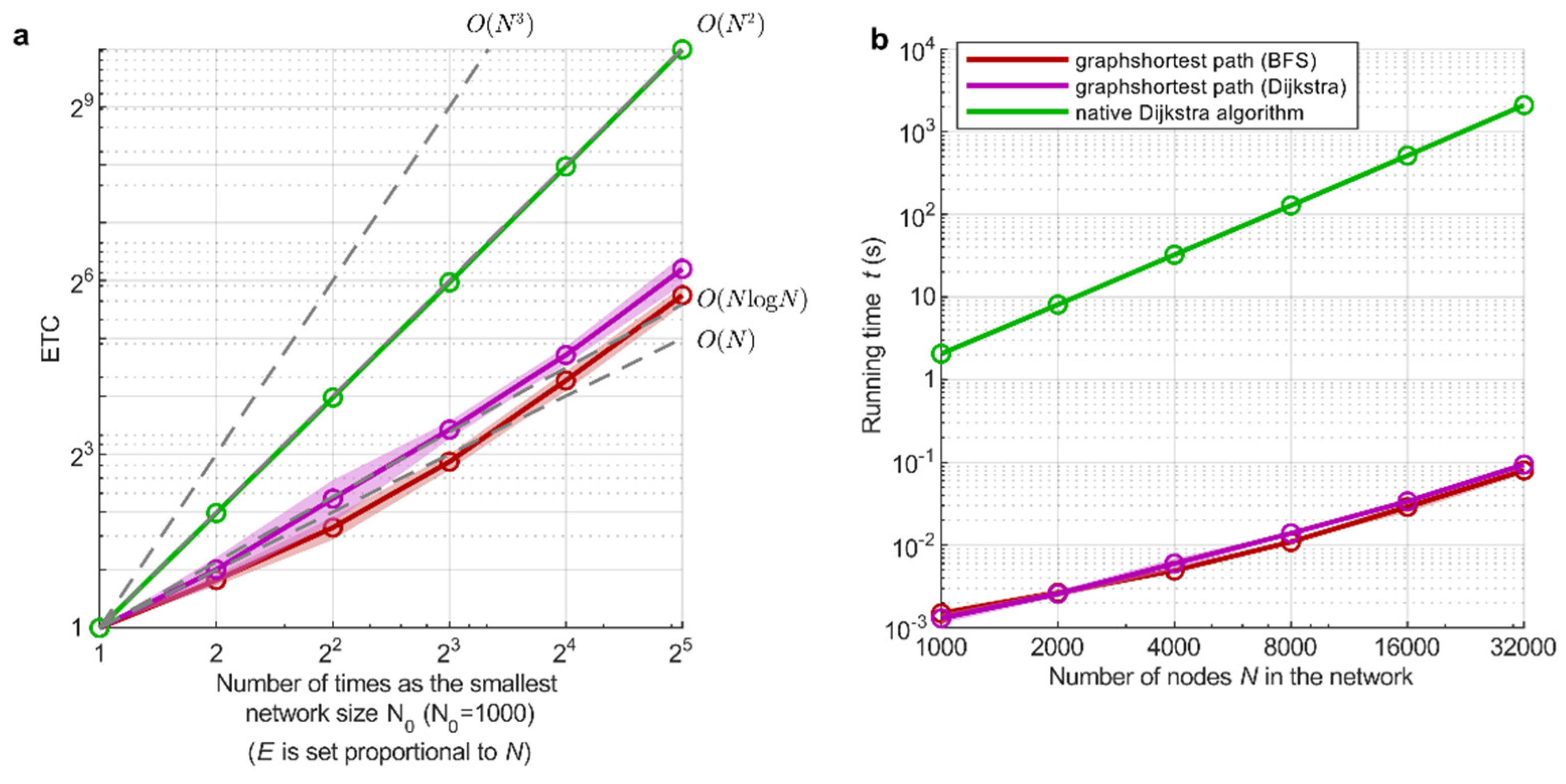
Figure 3. Empirical time complexity (ETC) and the running time of 3 square matrix multiplication algorithms in Matlab and Python. ETC in (a) of Matlab and (c) of Python was obtained by a normalization which divides the running time sequence in (b) and (d) by running time of the smallest matrix width respectively. The simulations were repeated for 6 times with the first repetition removed for stability, and normalization in ETC was performed repetition-wise. The mean of tested points (circle mark) and standard deviation (in shade) are shown. The gray dash lines in (a) and (c) are the ETC references of ideal complexity models with cubic, sub-cubic, square, and linear time complexity. The sub-cubic line

O (N^{2.807})

corresponds to the theoretical time complexity of Strassen’s algorithm, where

N

is the square matrix width.

Figure 3. Empirical time complexity (ETC) and the running time of 3 square matrix multiplication algorithms in Matlab and Python. ETC in (a) of Matlab and (c) of Python was obtained by a normalization which divides the running time sequence in (b) and (d) by running time of the smallest matrix width respectively. The simulations were repeated for 6 times with the first repetition removed for stability, and normalization in ETC was performed repetition-wise. The mean of tested points (circle mark) and standard deviation (in shade) are shown. The gray dash lines in (a) and (c) are the ETC references of ideal complexity models with cubic, sub-cubic, square, and linear time complexity. The sub-cubic line

O (N^{2.807})

corresponds to the theoretical time complexity of Strassen’s algorithm, where

N

is the square matrix width.

Disclaimer/Publisher’s Note: The statements, opinions and data contained in all publications are solely those of the individual author(s) and contributor(s) and not of MDPI and/or the editor(s). MDPI and/or the editor(s) disclaim responsibility for any injury to people or property resulting from any ideas, methods, instructions or products referred to in the content.

© 2025 by the authors. Licensee MDPI, Basel, Switzerland. This article is an open access article distributed under the terms and conditions of the Creative Commons Attribution (CC BY) license (http://creativecommons.org/licenses/by/4.0/).

Copyright: This open access article is published under a Creative Commons CC BY 4.0 license, which permit the free download, distribution, and reuse, provided that the author and preprint are cited in any reuse.

Empirical Time Complexity for Assessing the Algorithm Computational Consumption on a Hardware

Abstract

Keywords:

Subject:

Introduction

Results

ETC as a Visualization of Approximated TTC

ETC Reveals Practical Scalability Influenced by Crosstalk

Mathematical Proof for ETC as a Complexity Measure

Discussion

Materials and Methods

Empirical Time Complexity (ETC)

Counting Running Time of Algorithms

Matrix Multiplication

Hardware and Software Specifications

Author Contributions

Funding

Data Availability Statement

Acknowledgement

Conflicts of Interest

References

MDPI Initiatives

Important Links

Subscribe