Möbius Transformations in the Second Symmetric Product of ℂ

1. Introduction

In this paper, we translate the properties of the Möbius transformations of the Riemann sphere to the second symmetric product of the complex plane $\mathbb{C}$. That is, let T be a Möbius map, consider two complex numbers z, w, and consider the sets of the form $\left\{T\right(z),T(w\left)\right\}$, in the space $F_2\left(\mathbb{C}\right)=\{A\subset \mathbb{C}:|A|\le 2,A\ne \varnothing \}$, called the second symmetric product of the complex plane $\mathbb{C}$, which we will topologize through the Hausdorff metric, see [2] and [6].

To study the geometry of these transformations in this space, we introduced a model for $F_2\left(\mathbb{C}\right)$, that is, there is a homeomorphism from $F_2\left(\mathbb{C}\right)$ to a more suitable space in which we can have a better understanding of the geometry induced by $\{z,w\}\mapsto \left\{T\right(z),T(w\left)\right\}$, for any Möbius transformation T. The homeomorphic model of $F_2\left(\mathbb{C}\right)$ is the space

$${\mathbb{M}}_2=({\mathbb{R}}_{+}^3\times {\mathbb{S}}^1)/s,$$

where ${\mathbb{R}}_{+}^3=\{(x,y,z)\in {\mathbb{R}}^3:z\ge 0\}$ and s is a relation on elements of the form $(x,y,0,t)\in {\mathbb{R}}^3\times {\mathbb{S}}^1$, see [9].

Given $T\left(z\right)=(az+b)/(cz+d)$ a Möbius transformation in the Riemann sphere, we will define in the second symmetric space $F_2\left(\mathbb{C}\right)=\{s=\{z,w\}:z,w\in \mathbb{C}\}$, the function $\tilde{T}:F_2\left(\mathbb{C}\right)\to F_2\left(\mathbb{C}\right)$ given by $\tilde{T}\left(s\right)=\tilde{T}\left(\{z,w\}\right)=\{T\left(z\right),T\left(w\right)\}$, whenever T is defined in z and w. Recall that for $z=-d/c$, $T(-d/c)=\infty$, so we need to change the definition of $\tilde{T}$ when z or w are equal to $-d/c$; this change will produce discontinuities at some points, but on the other hand the change will be compatible to have some results similar to properties inherent in the set of Möbius transformations.

In Section 3, we define the set $M\left(F_2\left(\mathbb{C}\right)\right)=\{\tilde{T}:T\in Aut\left(\widehat{\mathbb{C}}\right)\}$, where each $\tilde{T}$ is taken with its corresponding domain and image. We look closely how the domains of these maps change depending on T and we describe the action of these maps via the usual generators of the group of Möbius transformations, describing in Propositions 2–5 the action of the generators in the space ${\mathbb{M}}_2$.

Some transitivity properties of the usual Möbius transformations can be translated on transitivity features of the set $M\left(F_2\left(\mathbb{C}\right)\right)$ in $F_2\left(\mathbb{C}\right)$. In Proposition 8, we prove that $M\left(F_2\left(\mathbb{C}\right)\right)$ is 2-transitive in $F_2\left(\mathbb{C}\right)$ if the corresponding points have the same cross ratio.

Now, if we consider the set of Euclidean circles and the family of lines in $\mathbb{C}$, the corresponding objects in ${\mathbb{M}}_2$ are Möbius strips and semi-planes, respectively. Proving first that $M\left(F_2\left(\mathbb{C}\right)\right)$ preserves these sets of Möbius strips and semi-planes, we show in Theorem 8, that $M\left(F_2\left(\mathbb{C}\right)\right)$ acts transitively in those sets. We also define maps that preserve the Möbius strips generated by Euclidean circles in $\mathbb{C}$ and prove some properties of these maps.

As any Möbius transformation T, different to the identity, is conjugated to a map of the form $U_{\lambda }\left(z\right)=\lambda z$ with $\lambda \in \mathbb{C}\setminus \{0,1\}$ or to the map $U_1\left(z\right)=z+1$, in Section 5, we extend this result for maps in the set $M\left(F_2\left(\mathbb{C}\right)\right)$ in Theorems 10, 11, and 12, depending if T is parabolic, hyperbolic or elliptic, respectively. Finally, we show how the corresponding maps to $U_{\lambda }$ in ${\mathbb{M}}_2$ act.

2. Preliminaries

In this section, we will briefly present the definitions and results about Möbius transformations and the second symmetric product of $\mathbb{C}$, that we will need in the rest of the paper.

2.1. Möbius Transformations

First, let us describe some basic facts about Möbius transformations, for more details, see [1] and [4]. Let $\widehat{\mathbb{C}}=\mathbb{C}\cup \{\infty \}$ be the Riemann sphere. We will denote by Aut$\left(\widehat{\mathbb{C}}\right)$ the set of all automorphisms of $\widehat{\mathbb{C}}$, that is, functions of the form

$$T\left(z\right)={\displaystyle \frac{az+b}{cz+d}},$$

with $a,b,c,d$ complex numbers such that $ad-bc\ne 0$. The transformations $w=T\left(z\right)$ are known as linear fractional or Möbius transformations. These transformations form a group under composition, where the inverse map of T is given by

$$T^{-1}\left(z\right)={\displaystyle \frac{dz-b}{-cz+a}}.$$

Moreover, as T does not determine the coefficients $a,b,c,d$ uniquely, since $\lambda a$, $\lambda b$, $\lambda c$, $\lambda d$ correspond to the same transformation T, for $\lambda \in \mathbb{C}\setminus \left\{0\right\}$, the group Aut$\left(\widehat{\mathbb{C}}\right)$ is isomorphic to the projective general linear group and to the projective special linear group, that is, Aut$\left(\widehat{\mathbb{C}}\right)\cong PGL(2,\mathbb{C})=PSL(2,\mathbb{C})$, thus from now on we can assume that $ad-bc=1$.

There are four special type of Möbius transformations that generate Aut$\left(\widehat{\mathbb{C}}\right)$:

$i)$ The map $R_{\theta }\left(z\right)=e^{i\theta }z$ ($\theta \in \mathbb{R})$ is a rotation of the Riemann sphere $\widehat{\mathbb{C}}$ by an angle $\theta$.

$ii)$ The transformation $J\left(z\right)=1/z$, that interchange 0 and ∞.

$iii)$ The map $S_r\left(z\right)=rz$ ($r\in \mathbb{R},r>0$) fixes 0 and ∞, and acts in the plane $\mathbb{C}$ as a similarity transformation.

$iv)$ The transformation $T_t\left(z\right)=z+t$ ($t\in \mathbb{C}$) fixes ∞ and acts as a translation in the complex plane.

One of the important properties of the group Aut$\left(\widehat{\mathbb{C}}\right)$ is that maps circles in $\widehat{\mathbb{C}}$ to circles in $\widehat{\mathbb{C}}$. In order to be more precise, the circles in $\widehat{\mathbb{C}}$ are the usual Euclidean circles and the straight lines in $\mathbb{C}$ (which can be thought as circles through infinity).

Theorem 1. If C is a circle in $\widehat{\mathbb{C}}$ and if $T\in$ Aut$\left(\widehat{\mathbb{C}}\right)$, then $T\left(C\right)$ is a circle in $\widehat{\mathbb{C}}$.

The group Aut$\left(\widehat{\mathbb{C}}\right)$ also has several properties about transitivity, the following are the ones we will use in this paper.

Theorem 2. If $(z_1,z_2,z_3)$ and $(w_1,w_2,w_3)$ are triples of distinct points in $\widehat{\mathbb{C}}$, then there is a unique $T\in$ Aut$\left(\widehat{\mathbb{C}}\right)$ such that $T\left(z_j\right)=w_j$, for $j=1,2,3$.

Corollary 1. If $T\in$ Aut$\left(\widehat{\mathbb{C}}\right)$ and T fixes three distinct points of $\widehat{\mathbb{C}}$, then T is the identity map.

Theorem 3. If C and $C^{\prime }$ are circles in $\widehat{\mathbb{C}}$, then there exists some $T\in$ Aut$\left(\widehat{\mathbb{C}}\right)$ such that $T\left(C\right)=C^{\prime }$.

In general Aut$\left(\widehat{\mathbb{C}}\right)$ is not 4-transitive, but if two 4-tuple of distinct points have the same cross ratio, there is some Möbius transformation that send one 4-tuple into the other. Recall that the cross ratio of four complex numbers is defined as $\lambda =(z_0,z_1;z_2,z_3)={\displaystyle \frac{(z_0-z_1)(z_2-z_3)}{(z_1-z_3)(z_3-z_0)}}$ with the convention of taking limits if some $z_j=\infty$.

Theorem 4. Let $(z_0,z_1,z_2,z_3)$ and $(w_0,w_1,w_2,w_3)$ be 4-tuples of distinct elements of $\widehat{\mathbb{C}}$. Then there exists some $T\in$ Aut$\left(\widehat{\mathbb{C}}\right)$ with $T\left(z_j\right)=w_j$, $j=0,1,2,3$ if and only if the two 4-tuples have the same cross ratio.

Consider a circle C in $\widehat{\mathbb{C}}$ given by the equation $az\overline{z}+bz+\overline{b}\overline{z}+c=0$, with $a,c\in \mathbb{R}$, $b\in \mathbb{C}$. If $a\ne 0$, then C is a Euclidean circle in the complex plane, and then there exists a transformation in the complex plane that fixes C. This transformation is given by

$$I_C\left(z\right)=-{\displaystyle \frac{\overline{b}\overline{z}+c}{a\overline{z}+b}}$$

and it is called the inversion in C. Moreover, if $T\in$ Aut$\left(\widehat{\mathbb{C}}\right)$, then $T\left(C\right)=C^{\prime }$ is another circle, then we have that $I_{C^{\prime }}=T{I}_C{T}^{-1}$.

To study the geometry of the Möbius transformations, there is a classification in conjugacy classes according to the number of fixed points and to the corresponding trace of the matrix associated in $PSL(2,\mathbb{C})$ to every map in Aut$\left(\widehat{\mathbb{C}}\right)$. The next results summarize this classification.

Theorem 5. Let $T\left(z\right)=(az+b)/(cz+d)$, with $ad-bc=1$. If ${(a+d)}^2\ne 4$, then T has two fixed points in $\widehat{\mathbb{C}}$; if ${(a+d)}^2=4$ and T is not the identity map, then T has one fixed point in $\widehat{\mathbb{C}}$.

For $\lambda \in \mathbb{C}\setminus \left\{0\right\}$, consider the maps $U_{\lambda }\left(z\right)=\lambda z$ if $\lambda \ne 1$ and $U_1\left(z\right)=z+1$. We will say that two maps T and S are conjugated if there exists another transformation V such that $T=V^{-1}\circ S\circ V$.

Theorem 6. Let T be a non-identity element in Aut$\left(\widehat{\mathbb{C}}\right)$, then there exists some $\lambda \in \mathbb{C}\setminus \left\{0\right\}$ such that T is conjugate to $U_{\lambda }$ in Aut$\left(\widehat{\mathbb{C}}\right)$.

Remark 1. When $\lambda =1$, the map T has only one fixed point $z_0$ and it is conjugated to $U_1\left(z\right)$ by a Möbius transformation S that sends $z_0$ to ∞. Since ${lim}_{n\to \infty }{U}_1^n\left(z\right)=\infty$, then any $z\in \mathbb{C}$ is moved by $T^n$ towards $z_0$ as n goes to infinity. In this case T is called parabolic.

Remark 2. If T in not parabolic, then it has two fixed points $z_1$ and $z_2$ and is conjugated to $U_{\lambda }$ with $\lambda \in \mathbb{C}\setminus \{0,1\}$, that fixes 0 and ∞, by means of a Möbius transformation S such that $S\left(z_1\right)=0$ and $S\left(z_2\right)=\infty$. If $\left|\lambda \right|<1$, ${lim}_{n\to \infty }{U}_{\lambda }^n\left(z\right)=0$ for all $z\ne \infty$ and hence ${lim}_{n\to \infty }{T}^n\left(z\right)=z_1$ for all $z\ne z_2$. In the same way if $\left|\lambda \right|>1$, then ${lim}_{n\to \infty }{T}^n\left(z\right)=z_2$ for all $z\ne z_1$ (the two cases for $\lambda$ are basically the same since we just replace $\lambda$ by $1/\lambda$). We conclude that if $\left|\lambda \right|\ne 1$, all points $z\ne z_1,z_2$ are moved by T away from one of these fixed points towards the other. If $\lambda >0$, T is called hyperbolic, and loxodromic otherwise. If $\left|\lambda \right|=1$, with $\lambda \ne 1$, then $U_{\lambda }$ is a rotation $R_{\theta }$, so $U_{\lambda }^n\left(z\right)$ has not limit for $z\ne 0,\infty$, hence neither $T^n\left(z\right)$ for $z\ne z_1,z_2$. In this case T is called elliptic.

2.2. Second Symmetric Product of $\mathbb{C}$

The second symmetric product of $\mathbb{C}$, denoted by $F_2\left(\mathbb{C}\right)$, is the set

$$F_2\left(\mathbb{C}\right)=\{A\subset \mathbb{C}:Ahasatmost2elementsandAisnotempty\};$$

The space $F_2\left(\mathbb{C}\right)$ has the topology induced by the following metric

$$\mathcal{H}(A,B)=inf\{\epsilon >0:A\subset {\mathcal{V}}_{\epsilon }\left(B\right)andB\subset {\mathcal{V}}_{\epsilon }\left(A\right)\},$$

where ${\mathcal{V}}_{\epsilon }\left(A\right)=\left\{x\in \mathbb{C}:d(x,A)<\epsilon \right\}$, $d(,)$ is the usual metric in $\mathbb{C}$, and A and B are subsets of $\mathbb{C}$. Given X a compact subset of $\mathbb{C}$, the space $F_2\left(X\right)$ can also be topologized through the Vietoris topology: if $U_1,\dots ,U_m$ are nonempty subsets of $\mathbb{C}$ and $m\in \mathbb{N}$, then define

$$\begin{array}{c}\langle U_1,\dots ,U_m\rangle =\{A\subset X:A\ne \varnothing ,\left|A\right|\le 2,A\subset \bigcup _{j=1}^m{U}_j\hfill \\ \hfill \mathrm{and}A\cap U_j\ne \varnothing ,\mathrm{for}\mathrm{all}j\in \{1,\dots ,m\}\};\end{array}$$

a base for the Vietoris topology is given by the family of the sets $\langle U_1,\dots ,U_m\rangle$, where $m\in \mathbb{N}$ and $U_1,\dots ,U_m$ are open subsets of $\mathbb{C}$. The Vietoris topology and the topology induced by the Hausdorff metric coincide in $F_2\left(\mathbb{C}\right)$.

Let X be a connected and compact subspace of $\mathbb{C}$. It is known that $F_2\left(X\right)$ is a continuum itself [7]. In [2] it is proven that, for $I=[0,1]$, $F_2\left(I\right)$ is homeomorphic to a 2-cell. In [6], it is proven that for the 1-sphere ${\mathbb{S}}^1$, $F_2\left({\mathbb{S}}^1\right)$ is homeomorphic to a Möbius strip.

2.3. A Model for $F_2\left(\mathbb{C}\right)$

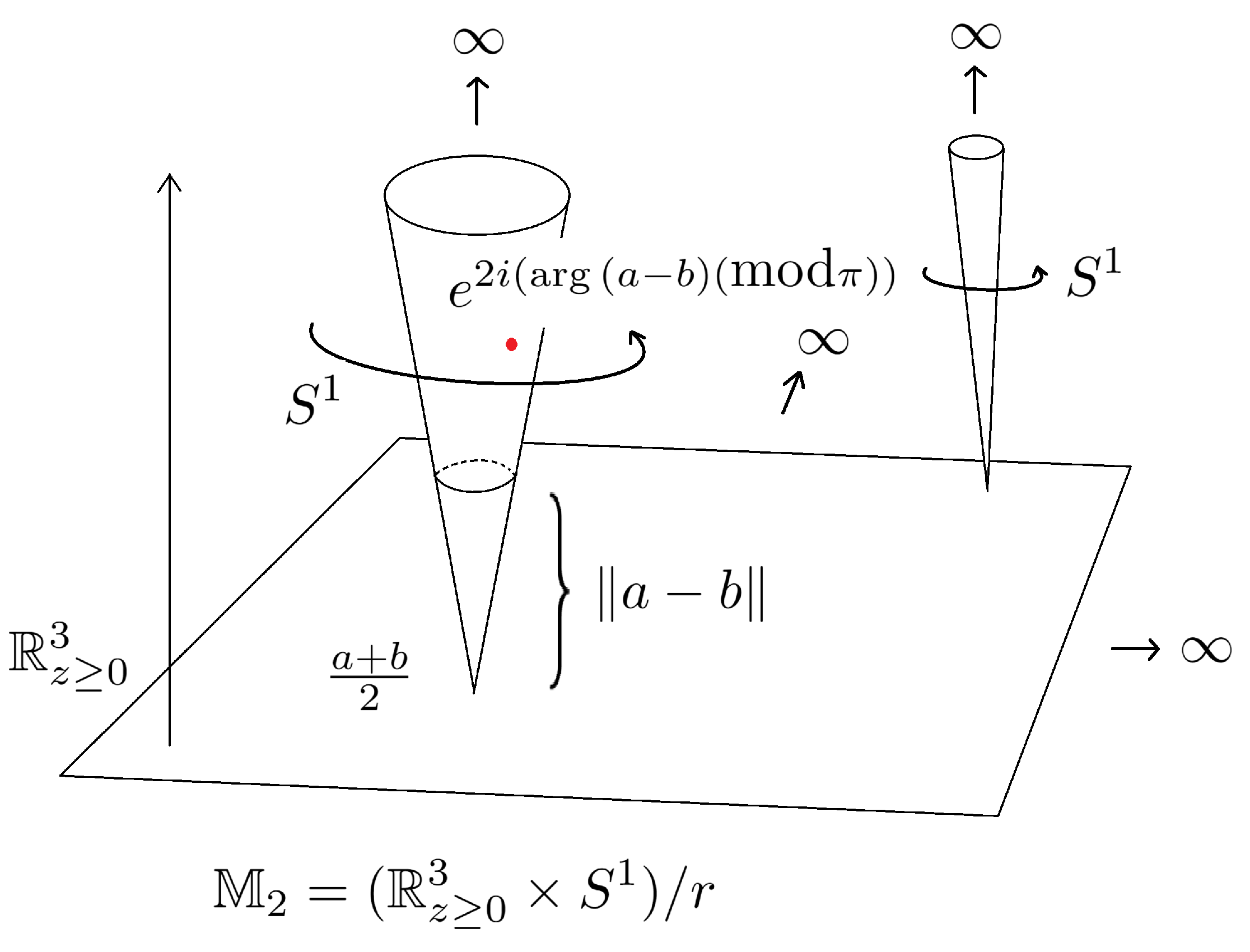
To have a better understanding of the space $F_2\left(\mathbb{C}\right)$, sometimes we will work in a model of $F_2\left(\mathbb{C}\right)$, that is, a continuous and bijective copy of $F_2\left(\mathbb{C}\right)$. Let ${\mathbb{M}}_2$ be the space $({\mathbb{R}}_{+}^3\times {\mathbb{S}}^1)/s$, where ${\mathbb{R}}_{+}^3=\{(x,y,z)\in {\mathbb{R}}^3:z\ge 0\}$, ${\mathbb{S}}^1$ the unit circle and such that s is a relation defined by $(x,y,0,t)\sim (x,y,0,t^{\prime })$, for all $t,t^{\prime }\in {\mathbb{S}}^1$.

Definition 1. Let $\Phi$ be the function $\Phi :F_2\left(\mathbb{C}\right)\to {\mathbb{M}}_2$ given by

$$\Phi \left(\{a,b\}\right)=\left\{\begin{array}{cc}\left({\displaystyle \frac{a+b}{2}},\parallel a-b\parallel ,e^{2i(arg(a-b)(mod\pi \left)\right)}\right),\hfill & ifa\ne b;\hfill \\ \left(class[a,0,t]\right),\hfill & ifa=b.\hfill \end{array}\right.$$

We observe that $\Phi$ is a well defined, bijective and bicontinuous function, with the corresponding topologies. We will call ${\mathbb{M}}_2$ the model of $F_2\left(\mathbb{C}\right)$.

Remark 3. Observe that given a point $(u,a,t)\in {\mathbb{M}}_2$, with $u\in {\mathbb{R}}^2$, $a\ge 0$ and $t\in {\mathbb{S}}^1$, we can obtain its preimage under $\Phi$ as follows: u must be the midpoint of two points $z_u$ and $w_u$ in the complex plane such that $\parallel z_u-w_u\parallel =a$ and $e^{2i\theta }=t$, where $\theta =arg(z_u-w_u)$, then $z_u$ and $w_u$ are points in the circle with center u and radius $a/2$, such that the segment $\overline{z_u{w}_u}$ is a diameter of the circle. Hence, $z_u=u+(a/2)e^{i\pi \theta }$ and $w_u=u-(a/2)e^{i\pi \theta }$.

In Figure 1, we can observe a representation of the model ${\mathbb{M}}_2$, for instance over any point $t={\displaystyle \frac{a+b}{2}}$, the midpoint of a, $b\in \mathbb{C}$, there is a cone V with vertex at t, so any two points z, $w\in \mathbb{C}$ with midpoint t has a representation in V at height $\parallel z-w\parallel$ and angle $e^{2i(arg(z-w)(mod\pi \left)\right)}$.

Let $\{x,y\}\in F_2\left(\mathbb{C}\right)$, observe that there exists a closed disk D, that contains x and y in its interior, then $\langle D\rangle \cap F_2\left(\mathbb{C}\right)$ is a neighborhood of $\{x,y\}$ in $F_2\left(\mathbb{C}\right)$. Given that $F_2\left(D\right)$ is a compact set, it follows that $F_2\left(\mathbb{C}\right)$ is a Hausdorff and a locally compact topological space, then it is possible to consider the Alexandroff’s compactification, denoted by $F_2(\mathbb{C}{)}^{*}$. The point added is denoted by ∞ (observe that this point will correspond to the pair of points $\{z,\infty \}$ in $F_2\left(\mathbb{C}\right)$, for each $z\in \mathbb{C})$). Note that in $F_2\left(\mathbb{C}\right)$ the sets $\{x,y\}$ such that $(x+y)/2=constant$ are mapped by $\Phi$ to a open topological disk, hence the Alexandroff’s compactification of such a set will be homeomorphic to ${\mathbb{S}}^2$. Moreover, observe that the singletons together with the point ∞ in $F_2(\mathbb{C}{)}^{*}$ is homeomorphic to ${\mathbb{S}}^2$.

3. Extension of the Möbius Transformations to the Space $F_2\left(\mathbb{C}\right)$

Let $T\left(z\right)=(az+b)/(cz+d)$ be a Möbius transformation in the Riemann sphere, let us define in the second symmetric space $F_2\left(\mathbb{C}\right)=\{a=\{z,w\}:z,w\in \mathbb{C}\}$, the function $\tilde{T}$ given by

$$\tilde{T}\left(a\right)=\tilde{T}\left(\{z,w\}\right)=\{T\left(z\right),T\left(w\right)\},z,w\ne -d/c.$$

(1)

In particular, observe that if $z=w$, then $\tilde{T}\left(a\right)=\tilde{T}\left(\left\{z\right\}\right)=\left\{T\left(z\right)\right\}$, hence the geometry of T in $\mathbb{C}$ will be reflected in $F_2\left(\mathbb{C}\right)$. As T has an inverse map $T^{-1}\left(z\right)=(dz-b)/(-cz+a)$, it is easy to see that in some appropriate domains ${\tilde{T}}^{-1}\circ \tilde{T}$ and $\tilde{T}\circ {\tilde{T}}^{-1}$ are the identity maps.

Observe that we can use the map $\Phi :F_2\left(\mathbb{C}\right)\to {\mathbb{M}}_2$, to translate the definition of T all the way to ${\mathbb{M}}_2$, that is, we can conjugate the map $\tilde{T}$ in some appropriate domain, via $\Phi$, to obtain a map $\widehat{T}$ in ${\mathbb{M}}_2$. So, from now on by convention, for any object X in $\mathbb{C}$, we will use $\tilde{X}$ for the object in $F_2\left(\mathbb{C}\right)$ generated by X, and $\widehat{X}$ for the corresponding object in the model ${\mathbb{M}}_2$.

Recall that a Möbius transformation T has at most two fixed points, and let us assume that T does not fix the point at infinity in the Riemann sphere. First, suppose that T has only one fixed point $z_0$, then the map $\tilde{T}$ has also $z_0$ as the only fixed point; meanwhile, if T fixes two distinct points $z_0$ and $z_1$, then $\tilde{T}$ has three fixed points: $\left\{z_0\right\},\left\{z_1\right\},\{z_0,z_1\}$.

As the map T is defined in $\widehat{\mathbb{C}}$, we need to consider the image and pre-image of the point at infinity, that is, $T(\infty )=a/c$ and $T(-d/c)=\infty$. Let us define the sets $D_T=F_2\left(\mathbb{C}\right)\setminus \{\{z,-d/c\}:z\in \mathbb{C}\}$ and $R_T=F_2\left(\mathbb{C}\right)\setminus \{\{z,a/c\}:z\in \mathbb{C}\}$, then we have our first result for the map $\tilde{T}$.

Lemma 1. For any $T\in$ Aut$\left(\widehat{\mathbb{C}}\right)$, the map $\tilde{T}:D_T\to R_T$ is an homeomorphism.

Proof. 

Assume that $T\left(z\right)=(az+b)/(cz+d)$. First, let us prove that $\tilde{T}$ is a bijection. Let $\{z_1,w_1\}$ and $\{z_2,w_2\}$ be two points in $D_T$, such that $\tilde{T}\left(\{z_1,w_1\}\right)=\tilde{T}\left(\{z_2,w_2\}\right)$, then it follows that $\{T\left(z_1\right),T\left(w_1\right)\}=\{T\left(z_2\right),T\left(w_2\right)\}$. If $z_1=w_1$, then $\{T\left(z_1\right),T\left(w_1\right)\}=\left\{T\left(z_1\right)\right\}=\{T\left(z_2\right),T\left(w_2\right)\}$ for which $T\left(z_1\right)=T\left(z_2\right)=T\left(w_2\right)$, therefore $z_1=z_2=w_2$; if now $z_1\ne w_1$, then $z_2\ne w_2$, and then $T\left(z_1\right)=T\left(z_2\right)$ or $T\left(z_1\right)=T\left(w_2\right)$; in the former case, $T\left(w_1\right)=T\left(w_2\right)$, and in the latter case, $T\left(z_2\right)=T\left(w_1\right)$. In any case, we have that $\{z_1,w_1\}=\{z_2,w_2\}$, since T is a one-to-one map, for which it follows the injectivity of $\tilde{T}$.

It is clear that for any pair of point $z,w\in \mathbb{C}$, neither equal to $a/c$, there are points $u,v\in \widehat{\mathbb{C}}$ such that $T\left(u\right)=z$ and $T\left(v\right)=w$, by the surjectivity of T, and therefore $\tilde{T}$ is onto. Now, observe that ${\tilde{T}}^{-1}:R_T\to D_T$ is the inverse map of $\tilde{T}$.

Finally, to establish the continuity of the map $\tilde{T}$ observe that $\tilde{T}\left(\left\{z\right\}\right)=\left\{T\left(z\right)\right\}$ and $\tilde{T}\left(\{z,w\}\right)=\{T\left(z\right),T\left(w\right)\}$, so by the continuity of T and the characterization of the open sets in the Hausdorff topology on $F_2\left(\mathbb{C}\right)$ we have the result. □

Observe that if $c=0$, then the map $\tilde{T}$ can be defined in all $F_2\left(\mathbb{C}\right)$ as in relation (1), and it is an homeomorphism there. For a general map $T\left(z\right)=(az+b)/(cz+d)$, we can think of the action of $\tilde{T}$ in $F_2\left(\mathbb{C}\right)$ as follows. For any $w\in \mathbb{C}$, we define the cone of vertex at w as the set $V_w=\{\{z,w\}:z\in \mathbb{C}\}\subset F_2\left(\mathbb{C}\right)$. Let $V_w^T=V_w\setminus \{-d/c,w\}$ and $V_w^{T*}=V_w\setminus \{a/c,w\}$. Then $\tilde{T}$ acts sending the cone $V_w^T$ with vertex at $w\ne -d/c$ one-to-one to the cone $V_{T\left(w\right)}^{T*}$ with vertex at $T\left(w\right)$, since $\tilde{T}\left(\{z,w\}\right)=\left(\{T\left(z\right),T\left(w\right)\}\right)\in V_{T\left(w\right)}$, for any $\{z,w\}\in V_w^T$. In fact, using the same arguments in the proof of Lemma 1, we have the following.

Lemma 2. Let $T\left(z\right)=(az+b)/(cz+d)$ be an element in Aut$\left(\widehat{\mathbb{C}}\right)$, then the map $\tilde{T}:V_w^T\to V_{T\left(w\right)}^{T*}$ is an homeomorphism, for any $w\ne -d/c$.

There are some special cones that need to be considered in the definition of $\tilde{T}$. Suppose that $z_0$ is a fixed point of T, then the cone $V_{z_0}^T$ is invariant under $\tilde{T}$, that is, $\tilde{T}$ is a homeomorphism from $V_{z_0}^T$ to $V_{z_0}^{T*}$; when T has two fixed points $z_1$ and $z_2$, the two cones $V_{z_1}$ and $V_{z_2}$ intersect each other in the other fixed point $\{z_1,z_2\}$ of $\tilde{T}$.

So far, we have defined $\tilde{T}$ only in $D_T$ (and then $\widehat{T}$ only in $\Phi \left(D_T\right)$), so we need to extend the definition of $\tilde{T}$. Observe that the set where we have not defined $\tilde{T}$ yet is precisely the cone $V_T:=V_{-d/c}=\{\{z,-d/c\}:z\in \mathbb{C}\}$, which will be called the singular cone for T, and the other cone $V_T^{\prime }=\{\{z,a/c\}:z\in \mathbb{C}\}$, will be called the singular value cone for T. For $\{z,-d/c\}\in V_T$, define the function $\tilde{T}$ as follows

$$\tilde{T}\left(\{z,-d/c\}\right)=\{T\left(z\right),a/c\}\in V_T^{\prime }.$$

(2)

Remark 4. Since T is bijective map in $\mathbb{C}$, we have that $\tilde{T}$ is a bijection from $V_T\setminus \{-d/c\}$ to $V_T^{\prime }\setminus \{a/c\}$. Also, observe that in the cone $\Phi \left(V_T\right)$, the map $\widehat{T}$ sends continuously circles at some particular height to topological circles in $\Phi \left(V_T^{\prime }\right)$. Moreover $\widehat{T}$ send points in the cone $\Phi \left(V_T\right)$ close to the vertex $-d/c$ to points in the cone $\Phi \left(V_T^{\prime }\right)$ close to infinity, and points in $V_T$ close to infinity to points in $V_T^{\prime }$ close to the vertex $a/c$.

In this way, we have defined $\tilde{T}$ in $V_T\setminus \{-d/c\}$, and therefore in all $F_2\left(\mathbb{C}\right)\setminus \{-d/c\}$ since $\tilde{T}$ was already defined in $D_T$. Moreover $\tilde{T}(V_T\setminus \{-d/c\})=V_T^{\prime }\setminus \{a/c\}$. Thus, we have extended the definition of $\tilde{T}$ to $F_2\left(\mathbb{C}\right)\setminus \{-d/c\}$ with image $F_2\left(\mathbb{C}\right)\setminus \{a/c\}$, so in a natural way we can extend the definition of $\tilde{T}$ to $F_2(\mathbb{C}{)}^{*}$, sending $\{-d/c\}\to \infty$ and $\infty \to a/c$. Using the notation that we have been using so far, we have the following result.

Theorem 7. Let $T\left(z\right)=(az+b)/(cz+d)$ be a Möbius transformation in the Riemann sphere. Then the map $\tilde{T}:F_2{\left(\mathbb{C}\right)}^{*}\to F_2{\left(\mathbb{C}\right)}^{*}$ is a bijective map, continuous in $D_T$ and continuous in $V_T$.

Proof. 

By Lemma 1, the map $\tilde{T}$ is an homeomorphism in $D_T$. As $\tilde{T}(V_T\setminus \{-d/c\})=V_T^{\prime }\setminus \{a/c\}$ in a bijective way by Equation (2), and $\{-d/c\}\to \infty$ and $\infty \to a/c$, we conclude that $\tilde{T}$ is a bijection. By Remark 4, we see that $\tilde{T}$ is continuous within $V_T$. □

Remark 5. Since by Lemma 1, the map $\tilde{T}:D_T\to R_T$ is an homeomorphism, any extension of the map in $V_T$ must has image $V_T^{\prime }$. If we consider a sequence of points $s_n=\{z_n,w_n\}\in D_T$ that converges to a point $\{z,-d/c\}$ in $V_T$ and consider the open set ${\mathcal{V}}_{\epsilon }\left(\{z,-d/c\}\right)$ in $F_2\left(\mathbb{C}\right)$ that contains the point $\{z,-d/c\}$, for some $ϵ>0$, then there exists $N\in \mathbb{N}$ such that if $n\ge N$, it follows that $s_n=\{z_n,w_n\}\in {\mathcal{V}}_{\epsilon }\left(\{z,-d/c\}\right)$. This means that for all $n\ge N$, $|z_n-z|<ϵ$ and $|w_n-(-d/c)|<ϵ$ or $|w_n-z|<ϵ$ and $|z_n-(-d/c)|<ϵ$, hence, there are sequences of complex points $\left\{a_n\right\}$, $\left\{b_n\right\}$ such that $a_n\to z$, $b_n\to -d/c$, as $n\to \infty$ and $\{a_n,b_n\}=\{z_n,w_n\}$ for $n\ge N$. As T is a continuous map, it follows that $T\left(b_n\right)\to T(-d/c)=\infty$, therefore we can not have continuity for the map $\tilde{T}$ when we approach $V_T$ from $D_T$.

Remark 6. It seems that we can use another compactification of $F_2\left(\mathbb{C}\right)$, different from Alexandroff’s compactification, in such a way the map $\tilde{T}$ is an homeomorphism in this new space, we just add a cone with vertex at infinity compatible with the topology of $F_2\left(\mathbb{C}\right)$; however we will lost the advantages to have the model for $F_2\left(\mathbb{C}\right)$ such as to be able to have a geometric description of the maps $\widehat{T}$. Another possible direction is to work in the second symmetric product of the Riemann sphere $F_2\left(\widehat{\mathbb{C}}\right)$, but we again lost the possible model to describe the geometry of the maps $\tilde{T}$.

Nevertheless, the map $\tilde{T}:F_2{\left(\mathbb{C}\right)}^{*}\to F_2{\left(\mathbb{C}\right)}^{*}$ is a bijective map, so we can define the set of transformations $M\left(F_2\left(\mathbb{C}\right)\right)=\{\tilde{T}:F_2{\left(\mathbb{C}\right)}^{*}\to F_2{\left(\mathbb{C}\right)}^{*}:T\in Aut\left(\widehat{\mathbb{C}}\right)\}$, where $\tilde{T}$ is defined as before, hence the set $M\left(F_2\left(\mathbb{C}\right)\right)$ is a group with the composition of maps as its group operation. In fact, if $T\left(z\right)=(az+b)/(cz+d)$ and $S\left(z\right)=(a^{\prime }z+b^{\prime })/(c^{\prime }z+d^{\prime })$ are two Möbius transformations, then we have that $\tilde{S}\circ \tilde{T}\left(\{z,w\}\right)=\{S\left(T\left(z\right)\right),S\left(T\left(w\right)\right)\}$ is well defined in all $F_2\left(\mathbb{C}\right)$. We will explore more about the structure of this group in a future manuscript.

3.1. Generators of $M\left(F_2\left(\mathbb{C}\right)\right)$

We will show now that all the maps in $M\left(F_2\left(\mathbb{C}\right)\right)$ are compositions of the following four maps:

$i)$${\tilde{R}}_{\theta }\left(\{z,w\}\right)=\{e^{i\theta }z,e^{i\theta }w\}$, $\theta \in \mathbb{R}$;

$ii)$$\tilde{J}\left(\{z,w\}\right)=\{1/z,1/w\}$, for $zw\ne 0$;

$iii)$${\tilde{S}}_r\left(\{z,w\}\right)=\{rz,rw\}$, $r\in \mathbb{R},r>0$;

$iv)$${\tilde{T}}_t\left(\{z,w\}\right)=\{z+t,w+t\}$, $t\in \mathbb{C}$.

Observe that ${\tilde{R}}_{\theta }$, ${\tilde{S}}_r$ and ${\tilde{T}}_t$ are homeomorphisms defined in all $F_2\left(\mathbb{C}\right)$, meanwhile $\tilde{J}$ is defined in all points $\{z,w\}\in F_2\left(\mathbb{C}\right)$, with $zw\ne 0$, but we can extend the definition of $\tilde{J}$ in its singular cone $V_J=\{\{z,0\}:z\in \mathbb{C}\}$ as in relation (2), that is, $\tilde{J}\left(\{z,0\}\right)=\{J\left(z\right),0\}$, for $z\ne 0$, and observe that for J its singular cone coincide with its singular value cone.

Proposition 1. Let S be a map in $M\left(F_2\left(\mathbb{C}\right)\right)$, then S can be expressed as a composition in some order of the maps ${\tilde{R}}_{\theta }$, ${\tilde{S}}_r$, ${\tilde{T}}_t$ and $\tilde{J}$.

Proposition Let $T\in$ Aut$\left(\widehat{\mathbb{C}}\right)$ such that $\tilde{T}=S$, and assume that $T\left(z\right)=(az+b)/(cz+d)$. If $c=0$, we know that $T=T_t\circ S_r\circ R_{\theta }$, where $b/d=t$ y $a/d=r{e}^{i\theta }$, hence it is straightforward to see that $S={\tilde{T}}_t\circ {\tilde{S}}_r\circ {\tilde{R}}_{\theta }$.

Now, when $c\ne 0$, $T\left(z\right)=(T_t\circ J)(-c^{2}z-cd)$, where $t=a/c$. By the first part of the proof, $-c^{2}z-cd=V\left(z\right)=T_{t^{\prime }}\circ S_r\circ R_{\theta }$, for some $t^{\prime }\in \mathbb{C}$, $r>0$ and $\theta \in \mathbb{R}$. Therefore $S={\tilde{T}}_t\circ \tilde{J}\circ \tilde{V}$. Note that the previous decomposition of $S=\tilde{T}$ even works for the singular cone $V_T$, take $\{z,-d/c\}\in V_T$, then ${\tilde{T}}_t\circ \tilde{J}\circ \tilde{V}\left(\{z,-d/c\}\right)={\tilde{T}}_t\left(\tilde{J}\left(\{V\left(z\right),V(-d/c)\}\right)\right)={\tilde{T}}_t\left(\tilde{J}\left(\{V\left(z\right),0\}\right)\right)={\tilde{T}}_t\left(\{J\left(V\left(z\right)\right),0\}\right)=\{J\left(V\left(z\right)\right)+a/c,a/c\}=\{T\left(z\right),a/c\}$.

Let us analyze the geometry of these generators maps in the space $F_2\left(\mathbb{C}\right)$. In order to do that, let us work in the model ${\mathbb{M}}_2$ of $F_2\left(\mathbb{C}\right)$. Since $\Phi :F_2\left(\mathbb{C}\right)\to {\mathbb{M}}_2$ is an homeomorphism we can conjugate any map $\tilde{F}:F_2\left(\mathbb{C}\right)\to F_2\left(\mathbb{C}\right)$ to a map $\widehat{F}:{\mathbb{M}}_2\to {\mathbb{M}}_2$, that is, $\Phi \circ \tilde{F}=\widehat{F}\circ \Phi$, extending the definition to infinity in a natural way. In particular, the elements of $M\left(F_2\left(\mathbb{C}\right)\right)$ can be thought acting in ${\mathbb{M}}_2$, so in some cases we will not make distinction if the context is clear.

Let us start with the map ${\tilde{R}}_{\theta }\left(\{z,w\}\right)=\{e^{i\theta }z,e^{i\theta }w\}$, $\theta \in \mathbb{R}$, and the analysis for the other maps will be similar. In this case, the conjugation gives a map ${\widehat{R}}_{\theta }$ such that $\Phi \circ {\tilde{R}}_{\theta }={\widehat{R}}_{\theta }\circ \Phi$; the left side composition satisfies that

$$\Phi ({\tilde{R}}_{\theta }\left(\{z,w\}\right)=\Phi \left(\{e^{i\theta }z,e^{i\theta }w\}\right)=\left(e^{i\theta }(z+w)/2,\parallel z-w\parallel ,e^{2i(arg{e}^{i\theta }(z-w)\left(mod\pi \right))}\right),$$

and the right side composition is equal to

$${\widehat{R}}_{\theta }\left(\Phi \left(\{z,w\}\right)\right)={\widehat{R}}_{\theta }\left((z+w)/2,\parallel z-w\parallel ,e^{2i(arg(z-w)(mod\pi \left)\right)}\right),$$

then the following result follows directly.

Proposition 2. The map ${\widehat{R}}_{\theta }:{\mathbb{M}}_2\to {\mathbb{M}}_2$ acts in the following way ${\widehat{R}}_{\theta }(u,l,t)=(e^{i\theta }u,l,e^{2i\theta }t)$, for $u\in {\mathbb{R}}^2$, $l\ge 0$ and $t\in {\mathbb{S}}^1$.

As a result we can determine the geometry of the map ${\tilde{R}}_{\theta }$ in $F_2\left(\mathbb{C}\right)$, stated as follows.

Corollary 2. The map ${\tilde{R}}_{\theta }$ acts conjugated as a double rotation with the same angle, in fact, this double rotation moves a point around a topological torus.

Proof. 

Just observe that since ${\tilde{R}}_{\theta }$ is conjugated to ${\widehat{R}}_{\theta }$, and by Proposition , ${\widehat{R}}_{\theta }(u,l,t)=(e^{i\theta }u,l,e^{2i\theta }t)$, the orbit of the point $(u,r,t)$ stays at the same height and the first and third coordinates are rotated by the same angle, so the result follows. □

In the same way, we can determine the action of corresponding maps ${\tilde{S}}_r$ and ${\tilde{T}}_t$ in the space ${\mathbb{M}}_2$.

Proposition 3. The map ${\widehat{S}}_r:{\mathbb{M}}_2\to {\mathbb{M}}_2$ acts as follows, ${\widehat{S}}_r(u,l,t)=(ru,rl,t)$, for $u\in {\mathbb{R}}^2$, $l\ge 0$ and $t\in {\mathbb{S}}^1$.

Proof. 

From the conjugation $\Phi \circ {\tilde{S}}_r={\widehat{S}}_r\circ \Phi$, we obtain that

$$\begin{array}{ccc}\hfill \Phi \left({\tilde{S}}_r\left(\{z,w\}\right)\right)& =& \Phi \left(\{rz,rw\}\right)=(r(z+w)/2,\parallel rz-rw\parallel ,e^{2i(arg(rz-rw)(mod\pi \left)\right)})\hfill \\ & =& (r(z+w)/2,r\parallel z-w\parallel ,e^{2i(argr+arg(z-w))\left(mod\pi \right))})\hfill \\ & =& {\widehat{S}}_r(\Phi \left(\{z,w\}\right)={\widehat{S}}_r((z+w)/2,\parallel z-w\parallel ,e^{2i(arg(z-w)(mod\pi \left)\right)}),\hfill \end{array}$$

from where it follows the claim, observing that $argr=0$. □

Using the definition in [8] of a topological attractor, we have the following.

Corollary 3. The point $O\in {\mathbb{M}}_2$ with coordinates $(0,0,0,1)$ is a fixed point of ${\widehat{S}}_r$, which is a global topological attractor for the dynamics of ${\widehat{S}}_r$, when $r<1$.

Proof. 

Remember that s is the relation defined by $(x,y,0,t)\sim (x,y,0,t^{\prime })$ for all $t,t^{\prime }$, so all points $(0,0,0,t)$ can be identified to the point $(0,0,0,1)$. Now it is clear that $O\in {\mathbb{M}}_2$ is a fixed point of ${\widehat{S}}_r$. By Proposition 3, the map ${\widehat{S}}_r$ is defined as ${\widehat{S}}_r(u,l,t)=(ru,rl,t)$, hence iterating this map, we obtain that ${\widehat{S}}_r^n(u,l,t)=(r^{n}u,r^{n}l,t)$, and since $r<1$, we obtain that ${\widehat{S}}_r^n(u,l,t)\to (0,0,0,1)$, as $n\to \infty$. □

Proposition 4. The map ${\widehat{T}}_t:{\mathbb{M}}_2\to {\mathbb{M}}_2$ acts in the following way ${\widehat{T}}_t(u,l,\theta )=(u+t,l,\theta )$, for $u\in {\mathbb{R}}^2$, $l\ge 0$ and $\theta \in {\mathbb{S}}^1$.

Proof. 

From the conjugation $\Phi \circ {\widehat{T}}_t={\widehat{T}}_t\circ \Phi$, we obtain that

$$\begin{array}{ccc}\hfill \Phi \left({\widehat{T}}_t\left(\{z,w\}\right)\right)& =& \Phi \left(\{z+t,w+t\}\right)=(((z+w)/2)+t,\parallel z-w\parallel ,e^{2i(arg(z-w)(mod\pi \left)\right)})\hfill \\ & =& {\widehat{T}}_t(\Phi \left(\{z,w\}\right)={\widehat{T}}_t((z+w)/2,\parallel z-w\parallel ,e^{2i(arg(z-w)(mod\pi \left)\right)}),\hfill \end{array}$$

from where it follows the claim. □

The next result follows directly from Proposition .

Corollary 4. The orbit of every point in ${\mathbb{M}}_2$ under the map ${\widehat{T}}_t$ goes to infinity.

Finally, let us analyze the action of the map $\widehat{J}$ in ${\mathbb{M}}_2$. Using the conjugation $\Phi \circ \tilde{J}=\widehat{J}\circ \Phi$, we get, first of all for $zw\ne 0$, that

$$\begin{array}{ccc}\hfill \Phi \circ \tilde{J}\left(\{z,w\}\right)& =& \Phi \left(\right\{1/z,1/w\left\}\right)\hfill \\ & =& (1/2(1/z+1/w),\parallel 1/z-1/w\parallel ,e^{2i(arg(1/z-1/w)(mod\pi \left)\right)})\hfill \\ & =& ((z+w)/2)·(1/\left(zw\right)),\parallel z-w\parallel /\parallel zw\parallel ,e^{2i(arg\left(\right(w-z)/zw)(mod\pi \left)\right)}).\hfill \end{array}$$

On the other hand, $\widehat{J}\circ \Phi \left(\{z,w\}\right)=\widehat{J}(((z+w)/2),\parallel z-w\parallel ,e^{2i(arg(z-w)(mod\pi \left)\right)})$, hence $\widehat{J}(u,l,t)=(u/\left(z_u{w}_u\right),l/(\parallel z_u{w}_u\parallel ),e^{-2iarg\left(z_u{w}_u\right)}t)$, where $u\in {\mathbb{R}}^2$, $l\ge 0$, $t\in {\mathbb{S}}^1$ and $z_u$, $w_u$ are the complex numbers that depends of u as in Remark 3.

In the cone $V_J=\{\{z,0\}:z\in \mathbb{C}\}$ we get that

$$\begin{array}{ccc}\hfill \Phi \circ \tilde{J}\left(\{z,0\}\right)=\Phi (\{1/z,0\}& =& (1/\left(2z\right),\parallel 1/z\parallel ,e^{2iarg(1/z)\left(mod\pi \right)})\hfill \\ & =& \widehat{J}\circ \Phi \left(\{z,0\}\right)=\widehat{J}(z/2,\parallel z\parallel ,e^{2i(arg\left(z\right)(mod\pi \left)\right)}).\hfill \end{array}$$

That is, $\widehat{J}(u,2\parallel u\parallel ,t)=(1/4u,1/(2\parallel u\parallel ),-t)$, for $u\in {\mathbb{R}}^2$ and $t=e^{2i(arg\left(2u\right))}$. In this way we can prove the following.

Proposition 5. The map $\widehat{J}:{\mathbb{M}}_2\to {\mathbb{M}}_2$ satisfy that $\widehat{J}\circ \widehat{J}=I{d}_{{\mathbb{M}}_2}$, the identity map in the model of $F_2\left(\mathbb{C}\right)$.

Proof. 

For $zw\ne 0$, we have that $\tilde{J}\circ \tilde{J}\left(\{z,w\}\right)=\left(\{J^2\left(z\right),J^2\left(w\right)\}\right)=\left(\{z,w\}\right)$, then as $\widehat{J}\circ \widehat{J}\circ \Phi =\Phi \circ \tilde{J}\circ \tilde{J}$, the result follows. In the cone $V_J$, just notice that $\tilde{J}\circ \tilde{J}\left(\{z,0\}\right)=\tilde{J}\left(\{J\left(z\right),0\}\right)=\tilde{J}\left(\{1/z,0\}\right)=\{z,0\}$, conjugating with the map $\Phi$ we have the result. □

4. Transitivity of $M\left(F_2\left(\mathbb{C}\right)\right)$

In this section we will prove several results about transitivity in the space $M\left(F_2\left(\mathbb{C}\right)\right)$. Let us start with two triples of distinct points in $\mathbb{C}$, that is, $(z_1,z_2,z_3)$ and $(w_1,w_2,w_3)$, then we can consider the triples of distinct points in $F_2\left(\mathbb{C}\right)$: $(\{z_1,z_2\},\{z_2,z_3\},\{z_3,z_1\})$ and $(\{w_1,w_2\},\{w_2,w_3\},\{w_3,w_1\})$. The first instance of transitivity is the following.

Proposition 6. If $(\{z_1,z_2\},\{z_2,z_3\},\{z_3,z_1\})$ and $(\{w_1,w_2\},\{w_2,w_3\},\{w_3,w_1\})$ are triples of distinct points in $F_2\left(\mathbb{C}\right)$, then there is a unique $\tilde{T}\in M\left(F_2\left(\mathbb{C}\right)\right)$ such that $\tilde{T}\left(\{z_i,z_j\}\right)=\{w_i,w_j\}$, for all $i,j\in \{1,2,3\}$, with $i\ne j$.

Proof. 

By Proposition 2, there is $T\in$ Aut$\left(\widehat{\mathbb{C}}\right)$ such that $T\left(z_i\right)=w_i$, for $i=1,2,3$, then $\tilde{T}\left(\{z_i,z_j\}\right)=\{w_i,w_j\}$, for all $i,j\in \{1,2,3\}$, with $i\ne j$.

Suppose there is another element $\tilde{S}$ in $M\left(F_2\left(\mathbb{C}\right)\right)$ such that $\tilde{S}\left(\{z_i,z_j\}\right)=\{w_i,w_j\}$. Consider the image of the first point, $\tilde{S}\left(\{z_1,z_2\}\right)=\{S\left(z_1\right),S\left(z_2\right)\}=\{w_1,w_2\}$, then there are two cases. If $S\left(z_1\right)=w_1$, then $S\left(z_2\right)=w_2$, and taking one of the other two points in $F_2\left(\mathbb{C}\right)$, we see that $S\left(z_3\right)=w_3$. By Proposition 2, we have that $S=T$ and then $\tilde{S}=\tilde{T}$. In case that $S\left(z_1\right)=w_2$, then $S\left(z_2\right)=w_1$, but we have that $\tilde{S}\left(\{z_2,z_3\}\right)=\{S\left(z_2\right),S\left(z_3\right)\}=\{w_2,w_3\}$ which is a contradiction since $S\left(z_2\right)=w_1$, this finish the proof of the uniqueness of the map $\tilde{T}$. □

Using the same argument as in the proof of the uniqueness in the previous result, we obtain the next Corollary.

Corollary 5. If $\tilde{T}\in M\left(F_2\left(\mathbb{C}\right)\right)$ fixes three distinct point of the form $\{z_1,z_2\},\{z_2,z_3\},\{z_3,z_1\}$, then $\tilde{T}$ is the identity map.

We can use again the 3-transitivity of Aut$\left(\widehat{\mathbb{C}}\right)$ and the arguments of the proof of Proposition 6 to prove the following result.

Proposition 7. Consider two pairs of points $\left\{z_0\right\}$, $\{z_1,z_2\}$ and $\left\{w_0\right\}$, $\{w_1,w_2\}$ in $F_2\left(\mathbb{C}\right)$ with $z_1\ne z_2$ and $w_1\ne w_2$, then there is a unique $\tilde{T}\in M\left(F_2\left(\mathbb{C}\right)\right)$ such that $\tilde{T}\left(\left\{z_0\right\}\right)=\left\{w_0\right\}$ and $\tilde{T}\left(\{z_1,z_2\}\right)=\{w_1,w_2\}$.

As a corollary we obtain that the Möbius transformations in $F_2\left(\mathbb{C}\right)$ act transitively in the set of cones $\mathcal{V}=\{V_a:V_a=\{\{z,a\}:z\in \mathbb{C}\}\}$.

Corollary 6. Let $\left\{z_0\right\}$ and $\left\{w_0\right\}$ be two singletons in $F_2\left(\mathbb{C}\right)$. Then there exists $\tilde{T}\in M\left(F_2\left(\mathbb{C}\right)\right)$ such that $\tilde{T}\left(V_{z_0}\right)=V_{w_0}$, that is, $M\left(F_2\left(\mathbb{C}\right)\right)$ is transitive in $\mathcal{V}$.

Proof. 

Consider different points $\{z_0,z_1\}$, $\{z_0,z_2\}\in V_{z_0}$ and $\{w_0,w_1\}$, $\{w_0,w_2\}\in V_{w_0}$, by the 3-transitivity of Aut$\left(\widehat{\mathbb{C}}\right)$ there exists a transformation $T\left(z\right)=(az+b)/(cz+d)$ such that $T\left(z_i\right)=w_i$ for $i=0,1,2$. Hence $\tilde{T}\left(\left\{z_0\right\}\right)=\left\{w_0\right\}$, $\tilde{T}\left(\{z_0,z_1\}\right)=\{w_0,w_1\}$ and $\tilde{T}\left(\{z_0,z_2\}\right)=\{w_0,w_2\}$. Let $\{z_0,z\}$ be a point in $V_{z_0}$, with $z\ne -d/c$, then $\tilde{T}\left(\{z_0,z\}\right)=\{T\left(z_0\right),T\left(z\right)\}=\{w_0,T\left(z\right)\}\in V_{w_0}$; for points $\{z_0,-d/c\}$, we get $\tilde{T}\left(\{z_0,-d/c\}\right)=\{T\left(z_0\right),a/c\}=\{w_0,a/c\}\in V_{w_0}$. □

For general points in $F_2\left(\mathbb{C}\right)$, we can prove 2-transitivity of the set $M\left(F_2\left(\mathbb{C}\right)\right)$ if these points combined have the same cross ratio.

Proposition 8. If $(\{z_1,z_2\},\{z_3,z_4\})$ and $(\{w_1,w_2\},\{w_2,w_3\})$ are pairs of distinct points in $F_2\left(\mathbb{C}\right)$, such that the cross ratio of $(z_1,z_2,z_3,z_4)$ is equal to the cross ratio of $(w_1,w_2,w_2,w_3)$, then there is $\tilde{T}\in M\left(F_2\left(\mathbb{C}\right)\right)$ such that $\tilde{T}\left(\{z_1,z_2\}\right)=\{w_1,w_2\}$ and $\tilde{T}\left(\{z_3,z_4\}\right)=\{w_3,w_4\}$.

Proof. 

By Proposition 2, there exists $T\in$ Aut$\left(\widehat{\mathbb{C}}\right)$ such that $T\left(z_i\right)=w_i$, for $i=1,2,3,4$, then $\tilde{T}\left(\{z_1,z_2\}\right)=\{w_1,w_2\}$ and $\tilde{T}\left(\{z_3,z_4\}\right)=\{w_3,w_4\}$. □

4.1. Transitivity of Möbius Bands

Let us consider $\mathcal{C}$ the family of Euclidean circles in $\mathbb{C}$ and $\mathcal{L}$ the family of lines in $\mathbb{C}$, remember that Aut$\left(\widehat{\mathbb{C}}\right)$ sends $\mathcal{C}\cup \mathcal{L}$ in itself, in fact, the action is transitive there.

We have observed that $F_2\left({\mathbb{S}}^1\right)$ is homeomorphic to a Möbius strip, then $F_2\left(C\right)$ is a Möbius band $\tilde{C}$, for any $C\in \mathcal{C}$. Moreover, passing to the model ${\mathbb{M}}_2$, we can see that $\Phi \left(\tilde{C}\right)=\widehat{C}$ is a Möbius band that intersects the subset $\{(x,y,0,0):(x,y,0,0)\in {\mathbb{M}}_2\}$ of ${\mathbb{M}}_2$ exactly in C.

It is not difficult to see that $F_2\left(L\right)$ is homeomorphic to a semi-plane $\widehat{L}$ in the model ${\mathbb{M}}_2$, for any $L\in \mathcal{L}$, in fact, $\widehat{L}\cap \{(x,y,0,0):(x,y,0,0)\in {\mathbb{M}}_2\}=L$.

Lemma 3. Let K be an element in $\mathcal{C}\cup \mathcal{L}$, then for any map S in $M\left(F_2\left(\mathbb{C}\right)\right)$, the set $S\left(\tilde{K}\right)$ is homeomorphic to a Möbius strip or homeomorphic to a semi-plane in the model ${\mathbb{M}}_2$.

Proof. 

Let S be an element of $M\left(F_2\left(\mathbb{C}\right)\right)$, then the corresponding map $T\in$Aut$\left(\widehat{\mathbb{C}}\right)$ (that is, $\tilde{T}=S$) satisfies that $T\left(K\right)$ is an Euclidean circle or a line in $\mathbb{C}$. Assume first that $K=C$ is an element of $\mathcal{C}$, the proof for the other case is similar. Passing to the model ${\mathbb{M}}_2$, consider the set $\widehat{T}\left(\widehat{C}\right)$.

First, if $T\left(C\right)$ is an Euclidean circle, then $\widehat{T\left(C\right)}$ is a Möbius band. Since $\Phi \circ \tilde{T}=\widehat{T}\circ \Phi$ and $\tilde{T}\left(\{z,w\}\right)=\{T\left(z\right),T\left(w\right)\}\in \tilde{T}\left(\tilde{C}\right)=\widetilde{T\left(C\right)}$, for any $z,w\in C$, it follows that $\widehat{T}\left(\widehat{C}\right)=\widehat{T}\left(\Phi \left(\tilde{C}\right)\right)=\Phi \left(\tilde{T}\left(\tilde{C}\right)\right)=\Phi \left(\widetilde{T\left(C\right)}\right)=\widehat{T\left(C\right)}$.

Now assume that $T\left(C\right)$ is a line in $\mathbb{C}$, this happens if $T\left(z\right)=(az+b)/(cz+d)$ and the point $-d/c$ is a point on C. Remember that in this case $\tilde{T}:D_T\to R_T$, and $\tilde{T}(V_T\setminus \{-d/c\})=V_T^{\prime }\setminus \{a/c\}$; then we only consider the image of $C^{\prime }=C\setminus \{-d/c\}$, that is, $T\left(C^{\prime }\right)$ is a complete line since $T(-d/c)=\infty$. It follows that $\widehat{T\left(C^{\prime }\right)}$ still is a whole semi-plane and once again, using that $\tilde{T}\left({\tilde{C}}^{\prime }\right)=\widetilde{T\left(C^{\prime }\right)}$, we get that $\widehat{T}\left({\widehat{C}}^{\prime }\right)=\widehat{T\left(C^{\prime }\right)}$, which conclude the proof. □

Now we will prove transitivity for a family of Möbius strips in ${\mathbb{M}}_2$. Consider the set $M_{\mathcal{C}\cup \mathcal{L}}=\{\Phi \left(F_2\left(K\right)\right):K\in \mathcal{C}\cup \mathcal{L}\}$, that is, $M_{\mathcal{C}\cup \mathcal{L}}$ consists of Möbius bands and semi-planes generated by Euclidean circles and lines in $\mathbb{C}$, respectively.

Theorem 8. The set $M\left(F_2\left(\mathbb{C}\right)\right)$ acts transitively on $M_{\mathcal{C}\cup \mathcal{L}}$, that is, if ${\widehat{K}}_1$, ${\widehat{K}}_2\in M_{\mathcal{C}\cup \mathcal{L}}$, then there exists $\tilde{S}\in M\left(F_2\left(\mathbb{C}\right)\right)$ such that $\widehat{S}\left({\widehat{K}}_1\right)={\widehat{K}}_2$.

Proof. 

Let ${\widehat{K}}_1$ and ${\widehat{K}}_2$ be two elements in $M_{\mathcal{C}\cup \mathcal{L}}$. Let $\{z_1,w_1\}$, $\{z_2,w_2\}$ be two different points in ${\tilde{K}}_1$ and let $\{u_1,v_1\}$, $\{u_2,v_2\}$ be two different points in ${\tilde{K}}_2$, then $z_1,w_1,z_2,w_2$ are in the same Euclidean circle or in the same line $K_1$ in $\mathbb{C}$, that generates the Möbius strip or the semi-plane ${\widehat{K}}_1$, and the same holds for $u_1,v_1,u_2,v_2$, they are in the same Euclidean circle or in the same line $K_2$ in $\mathbb{C}$, that generates the Möbius strip or the semi-plane ${\widehat{K}}_2$.

Notice that since $\{z_1,w_1\}$, $\{z_2,w_2\}$ are different, then there are at least three different complex numbers in the set $A=\{z_1,w_1,z_2,w_2\}$, and the same happens in the set $B=\{u_1,v_1,u_2,v_2\}$. By Proposition 2 there is a unique Möbius transformation S that sends the three different points in A into the three different points in B. Since three points suffice to determine a circle or a line, then $S\left(K_1\right)=K_2$, thus $\tilde{S}\left({\tilde{K}}_1\right)={\tilde{K}}_2$ and the result follows. □

The next result characterize the sets in $M_{\mathcal{C}\cup \mathcal{L}}$ using cross ratio.

Corollary 7. Let $\widehat{K}$ be an element in $M_{\mathcal{C}\cup \mathcal{L}}$ and let $\{z_0,w_0\}$ be a point in $\tilde{K}$. Then $\tilde{K}=\{\{z,w\}:(z_0,w_0;z,w)\in \mathbb{R}\cup \{\infty \}\}$.

Proof. 

First, observe that $\mathbb{R}$ is a line in $\mathbb{C}$. The set $\tilde{K}$ is generated by an Euclidean circle or a line K in $\mathbb{C}$. Let T be the Möbius transformation such that $T\left(K\right)=\mathbb{R}\cup \{\infty \}$, then if $\{z,w\}\in \tilde{K}$ it follows that $T\left(z_0\right),T\left(w_0\right),T\left(z\right),T\left(w\right)\in \mathbb{R}\cup \{\infty \}$. By Theorem 2, $(z_0,w_0;z,w)=(T\left(z_0\right),T\left(w_0\right);T\left(z\right),T\left(w\right))$ and the result follows. □

4.2. Inversion in Möbius strips

Let C be a circle in $\widehat{\mathbb{C}}$ given by the equation $az\overline{z}+bz+\overline{b}\overline{z}+c=0$, with $a,c\in \mathbb{R}$, $b\in \mathbb{C}$. If $a\ne 0$, then C is a Euclidean circle in the complex plane, and then there exists a transformation in the complex plane that fixes C, such transformation is given by

$$I_C\left(z\right)=-{\displaystyle \frac{\overline{b}\overline{z}+c}{a\overline{z}+b}},$$

(3)

and it is called the inversion in C. This transformation fixes point-wise the set C, sends the center of C to infinity and vice versa, and $I_C\circ I_C$ is the identity map. Moreover, if $T\in$ Aut$\left(\widehat{\mathbb{C}}\right)$, then $T\left(C\right)=C^{\prime }$ is another circle and we have that $I_{C^{\prime }}=T{I}_C{T}^{-1}$.

Given an Euclidean circle C in $\mathbb{C}$, we have that $F_2\left(C\right)$ is homeomorphic to a Möbius strip, for which we can define its inversion as follows. Let $\widehat{C}$ be the corresponding Möbius band in the model ${\mathbb{M}}_2$, and let ${\widehat{I}}_C:{\mathbb{M}}_2\to {\mathbb{M}}_2$ given by $\Phi \circ {\tilde{I}}_C={\widehat{I}}_C\circ \Phi$, where ${\tilde{I}}_C:F_2\left(\mathbb{C}\right)\to F_2\left(\mathbb{C}\right)$ is given by ${\tilde{I}}_C\left(\{z,w\}\right)=\{I_C\left(z\right),I_C\left(w\right)\}$, for $z,w\ne -\overline{b}/a$, and ${\tilde{I}}_C\left(\{z,-\overline{b}/a\}\right)=\{I_C\left(z\right),-\overline{b}/a\}$, where $-\overline{b}/a$ is the center of C. We call the map ${\widehat{I}}_C$ the inversion in the Möbius band $\widehat{C}$. Then we have the following properties for the map ${\widehat{I}}_C$, taking $I_C$ as in (3) from now on.

Proposition 9. The map ${\widehat{I}}_C$ fixes point-wise the Möbius strip $\widehat{C}$ and ${\widehat{I}}_C\circ {\widehat{I}}_C$ is the identity map in ${\mathbb{M}}_2$.

Proof. 

As $I_C$ fixes the set C point-wise, it follows that ${\tilde{I}}_C\left(\{z,w\}\right)=\{I_C\left(z\right),I_C\left(w\right)\}=\{z,w\}$ if $z,w\in C$. Thus $\Phi \left(\{z,w\}\right)=\Phi \circ {\tilde{I}}_C\left(\{z,w\}\right)={\widehat{I}}_C\circ \Phi \left(\{z,w\}\right)$, we conclude that ${\widehat{I}}_C$ fixes $\widehat{C}$ point-wise.

The second statement follows from the fact that ${\tilde{I}}_C\circ {\tilde{I}}_C\left(\{z,w\}\right)=\{I_C\circ I_C\left(z\right),I_C\circ I_C\left(w\right)\}=\{z,w\}$, for any $z,w\in \mathbb{C}\setminus \{-\overline{b}/a\}$; and ${\tilde{I}}_C\circ {\tilde{I}}_C\left(\{z,-\overline{b}/a\}\right)={\tilde{I}}_C\left(\{I_C\left(z\right),-\overline{b}/a\}\right)=\{I_C\left(I_C\left(z\right)\right),-\overline{b}/a\}=\{z,-\overline{b}/a\}$. □

Remark 7. For any complex number z we know that $I_C\circ I_C\left(z\right)=z$, then it follows that $\{z,I_C\left(z\right)\}$ is a fixed point for ${\tilde{I}}_C$, that is, ${\tilde{I}}_C$ not only fixes the Möbius strip $\tilde{C}$, but has infinitely many other fixed points. Observe that these points correspond to infinite rays coming out from the manifold boundary of the fixed Möbius strip; and these rays do not intersect. Therefore, the fixed set is homeomorphic to a real projective plane minus a point. Moreover, every point $\{z,w\}$ in $F_2\left(\mathbb{C}\right)$ is a fixed point or a periodic point of period 2 under ${\tilde{I}}_C$.

Now let us consider two Möbius bands $\widehat{C}$, $\widehat{C^{\prime }}$ in $M_{\mathcal{C}\cup \mathcal{L}}$, so we know that there is a Möbius transformation T such that $T\left(C\right)=C^{\prime }$, then the next result follows.

Proposition 10. The inversions ${\widehat{I}}_C$ and ${\widehat{I}}_{C^{\prime }}$ of two Möbius bands $\widehat{C}$ and $\widehat{C^{\prime }}$ in $M_{\mathcal{C}\cup \mathcal{L}}$, respectively, are conjugated in the subset ${\mathbb{M}}_2\setminus \Phi (V_T\cup V_T^{\prime })$ of ${\mathbb{M}}_2$.

Proof. 

Just observe that there is a Möbius transformation $T\left(z\right)=(az+b)/(cz+d)$ such that $T\left(C\right)=C^{\prime }$. Since $I_{C^{\prime }}=T{I}_C{T}^{-1}$, it follows that ${\tilde{I}}_{C^{\prime }}=\tilde{T}\circ {\tilde{I}}_C\circ {\tilde{T}}^{-1}$ in $F_2\left(\mathbb{C}\right)\setminus (V_T\cup V_T^{\prime })$, and then after conjugating with $\Phi$ we obtain ${\widehat{I}}_{C^{\prime }}=\widehat{T}\circ {\widehat{I}}_C\circ {\widehat{T}}^{-1}$, in ${\mathbb{M}}_2\setminus \Phi (V_T\cup V_T^{\prime })$. □

Note that we can extend the conjugation to $V_T^{\prime }$, since we must have that $\tilde{T}\circ {\tilde{I}}_C\circ {\tilde{T}}^{-1}\left(\{z,a/c\}\right)=\tilde{T}\left({\tilde{I}}_C\left(\{T^{-1}\left(z\right),-d/c\}\right)\right)=\tilde{T}\left(\{I_C\left(T^{-1}\left(z\right)\right),I_C(-d/c)\}\right)=\{T\left(I_C\left(T^{-1}\left(z\right)\right)\right),T\left(I_C(-d/c)\right)\}=\{I_{C^{\prime }}\left(z\right),T\left(I_C(-d/c)\right)\}$, and then use the map $\Phi$. Notice that when $C^{\prime }$ is a line we have that $-d/c\in C^{\prime }$, then $\tilde{T}\circ {\tilde{I}}_C\circ {\tilde{T}}^{-1}\left(\{z,a/c\}\right)=\{I_{C^{\prime }}\left(z\right),a/c\}$.

In particular, consider the real line $\mathbb{R}$, then for any Euclidean circle C, we can send C to $\mathbb{R}\cup \{\infty \}$ by a Möbius transformation $T\left(z\right)=(az+b)/(cz+d)$, then the point $-d/c\in C$ since $T(-d/c)=\infty$. Thus $I_{\mathbb{R}}=T{I}_C{T}^{-1}$, where $I_{\mathbb{R}}\left(z\right)=\overline{z}$. In $F_2\left(\mathbb{C}\right)\setminus V_T^{\prime }$, we get that $\tilde{T}\circ {\tilde{I}}_C\circ {\tilde{T}}^{-1}={\tilde{I}}_{\mathbb{R}}$, and $\tilde{T}\circ {\tilde{I}}_C\circ {\tilde{T}}^{-1}:V_T^{\prime }\to V_T^{\prime }$, since $\tilde{T}\circ {\tilde{I}}_C\circ {\tilde{T}}^{-1}\left(\{z,a/c\}\right)=\tilde{T}\left({\tilde{I}}_C\left(\{T^{-1}\left(z\right),-d/c\}\right)\right)=\tilde{T}\left(\{I_C\left(T^{-1}\left(z\right)\right),I_C(-d/c)\}\right)=\tilde{T}\left(\{I_C\left(T^{-1}\left(z\right)\right),-d/c\}\right)=\{T\left(I_C\left(T^{-1}\left(z\right)\right)\right),a/c\}=\{\overline{z},a/c\}$, where $I_C(-d/c)=-d/c$ as $-d/c\in C$. In this way, we have defined the conjugation in all $F_2\left(\mathbb{C}\right)$ and then we can pass to ${\mathbb{M}}_2$.

Theorem 9. For any $\widehat{C}$ element in $M_{\mathcal{C}\cup \mathcal{L}}$, the inversion in $\widehat{C}$ is conjugated to the map ${\widehat{I}}_{\mathbb{R}}:{\mathbb{M}}_2\to {\mathbb{M}}_2$, given by ${\widehat{I}}_{\mathbb{R}}(u,r,\theta )=(\overline{u},r,-\theta )$, for $u\in {\mathbb{R}}^2$, $r\ge 0$ and $\theta \in {\mathbb{S}}^1$.

Proof. 

Let T be the Möbius transformation such that $T\left(C\right)=\mathbb{R}$, and we assume that C is an Euclidean circle, the case when C is a line is similar. Since $I_{\mathbb{R}}=T{I}_C{T}^{-1}$, it follows that the map ${\tilde{I}}_{\mathbb{R}}=\tilde{T}\circ {\tilde{I}}_C\circ {\tilde{T}}^{-1}$ is defined in $F_2\left(\mathbb{C}\right)\setminus V_T^{\prime }$ as ${\tilde{I}}_{\mathbb{R}}\left(\{z,w\}\right)=\{I_{\mathbb{R}}\left(z\right),I_{\mathbb{R}}\left(w\right)\}=\{\overline{z},\overline{w}\}$. Thus ${\widehat{I}}_{\mathbb{R}}=\widehat{T}\circ {\widehat{I}}_C\circ {\widehat{T}}^{-1}$ is defined in ${\mathbb{M}}_2\setminus \Phi \left(V_T^{\prime }\right)$, using the conjugation $\Phi \circ {\tilde{I}}_{\mathbb{R}}={\widehat{I}}_{\mathbb{R}}\circ \Phi$, we obtain that

$$\begin{array}{ccc}\hfill \Phi \circ {\tilde{I}}_{\mathbb{R}}\left(\{z,w\}\right)=\Phi \left(\{\overline{z},\overline{w}\}\right)& =& ((\overline{z}+\overline{w})/2,\parallel \overline{z}-\overline{w}\parallel ,e^{2i(arg(\overline{z}-\overline{w})\left(mod\pi \right))})\hfill \\ & =& ((\overline{z}+\overline{w})/2,\parallel z-w\parallel ,e^{2i(-arg(z-w)(mod\pi \left)\right)}),\hfill \end{array}$$

is equal to ${\widehat{I}}_{\mathbb{R}}\circ \Phi \left(\{z,w\}\right)={\widehat{I}}_{\mathbb{R}}((z+w)/2,\parallel z-w\parallel ,e^{2i(arg(z-w)(mod\pi \left)\right)})$, and the result follows in ${\mathbb{M}}_2\setminus \Phi \left(V_T^{\prime }\right)$.

To complete the proof, observe that for points $\{z,a/c\}\in V_T^{\prime }$, we get that

$${\widehat{I}}_{\mathbb{R}}((z+a/c)/2,\parallel z-a/c\parallel ,e^{2i(arg(z-a/c)(mod\pi \left)\right)})$$

$$=((\overline{z}+a/c)/2,\parallel \overline{z}-a/c\parallel ,e^{2i(arg(\overline{z}-a/c)\left(mod\pi \right))}),$$

but since $a,c\in \mathbb{R}$, then $\parallel z-a/c\parallel =\parallel \overline{z}-a/c\parallel$, $\overline{(z+a/c)/2}=(\overline{z}+a/c)/2$ and $arg(z-a/c)=-arg(\overline{z}-a/c)$, so we can conclude that for $(u,r,\theta )\in \Phi \left(V_T^{\prime }\right)$ it follows that ${\widehat{I}}_{\mathbb{R}}(u,r,\theta )=(\overline{u},r,-\theta )$, as well. □

5. Conjugacy Classes in $M\left(F_2\left(\mathbb{C}\right)\right)$

For $\lambda \in \mathbb{C}\setminus \left\{0\right\}$, consider the maps $U_{\lambda }\left(z\right)=\lambda z$ if $\lambda \ne 1$ and $U_1\left(z\right)=z+1$, otherwise; all these maps are elements in Aut$\left(\widehat{\mathbb{C}}\right)$. Then, if T is a non-identity element in Aut$\left(\widehat{\mathbb{C}}\right)$, then T is conjugate to $U_{\lambda }$ for some $\lambda \in \mathbb{C}\setminus \left\{0\right\}$. In this section we will extend this result for maps in $M\left(F_2\left(\mathbb{C}\right)\right)$, starting with the case $\lambda =1$.

5.1. Parabolic Maps

Let $T\left(z\right)=(az+b)/(cz+d)$ be a Möbius transformation with only one fixed point at $z_0$, then T is called a parabolic transformation and it is conjugated to the map $U_1\left(z\right)=z+1=T_1\left(z\right)$. Let S be the Möbius transformation that conjugates T and $T_1$, remember that $S\left(z_0\right)=\infty$, so $S\left(z\right)=t/(z-z_0)$ for some $t\in \mathbb{C}\setminus 0$. In order to see the conjugation in $F_2\left(\mathbb{C}\right)$, we need to consider the singular cones of T and S.

First, consider the singular cone of S, that is, $V_S$ that coincide with the cone $V_{z_0}$, then $\tilde{S}:V_S\to V_0$ is given by $\tilde{S}\left(\{z,z_0\}\right)=\{S\left(z\right),0\}$. So the conjugation $\tilde{S}\circ \tilde{T}={\tilde{T}}_1\circ \tilde{S}$ in $V_{z_0}$ is given by $\tilde{S}\circ \tilde{T}\left(\{z,z_0\}\right)=\tilde{S}\left(\{T\left(z\right),z_0\}\right)=\{S\left(T\left(z\right)\right),0\}={\tilde{T}}_1\left(\{S\left(z\right),0\}\right)$, then we defined ${\tilde{T}}_1$ in $V_0$ as ${\tilde{T}}_1\left(\{z,0\}\right)=\{z+1,0\}$. Similarly, in the singular cone $V_T$ of T, we have that, $\tilde{S}\circ \tilde{T}\left(\{z,-d/c\}\right)=\tilde{S}\left(\{T\left(z\right),a/c\}\right)=\{S\left(T\left(z\right)\right),S(a/c)\}$, and the last quantity we would like to be equal to ${\tilde{T}}_1\left(\{S\left(z\right),S(-d/c)\}\right)$, then we define ${\tilde{T}}_1\left(\{z,S(-d/c)\}\right)=\{z+1,S(a/c)\}$ in $V_{S(-d/c)}$.

In any other cone $V_z\subset F_2\left(\mathbb{C}\right)$, with $z\ne z_0,-d/c$, we have that $\tilde{S}\circ \tilde{T}={\tilde{T}}_1\circ \tilde{S}$, in $V_z\setminus \{\{z,z_0\},\{z,-d/c\}\}$, that is, ${\tilde{T}}_1\left(\{z,w\}\right)=\{z+1,w+1\}$. Using the relation $\Phi \circ {\tilde{T}}_1={\widehat{T}}_1\circ \Phi$, we can conjugate the action of $\tilde{T}$ in $F_2\left(\mathbb{C}\right)$ to the action of ${\widehat{T}}_1$ in ${\mathbb{M}}_2$.

Remark 8. In $V_0$, we obtain that

$$\begin{array}{cc}\Phi \circ {\tilde{T}}_1\left(\{z,0\}\right)\hfill & =\Phi (\left(\{z+1,0\}\right)=((z+1)/2,\parallel z+1\parallel ,e^{2i(arg(z+1)(mod\pi \left)\right)})\hfill \\ & ={\widehat{T}}_1\circ \Phi \left(\{z,0\}\right)={\widehat{T}}_1\left(\right(z/2,\parallel z\parallel ,e^{2i(arg\left(z\right)(mod\pi \left)\right)}).\hfill \end{array}$$

Remark 9. Meanwhile in $V_{S(-d/c)}$, we get, setting $w=S(-d/c)$ and $v=S(a/c)$

$$\begin{array}{ccc}\hfill \Phi \circ {\tilde{T}}_1\left(\{z,w\}\right)& =& \Phi (\left(\{z+1,v\}\right)=((z+1+v)/2,\parallel z+1-v\parallel ,e^{2i(arg(z+1-v)(mod\pi \left)\right)})\hfill \\ & =& {\widehat{T}}_1\circ \Phi \left(\{z,w\}\right)={\widehat{T}}_1((z+w)/2,\parallel z-w\parallel ,e^{2i(arg(z-w)(mod\pi \left)\right)}).\hfill \end{array}$$

Setting ${\mathbb{M}}_2^p={\mathbb{M}}_2\setminus \Phi (V_0\cup V_{S(-d/c)})$ we get the following result.

Theorem 10. Let $W\in M\left(F_2\left(\mathbb{C}\right)\right)$ be a map with only one fixed point, then W is conjugated to the map ${\widehat{T}}_1:{\mathbb{M}}_2^p\to {\mathbb{M}}_2$ given by ${\widehat{T}}_1(u,r,\theta )=(u+1,r,\theta )$, for $u\in {\mathbb{R}}^2$, $r\ge 0$ and $\theta \in {\mathbb{S}}^1$.

Proof. 

As W has only one fixed point in $F_2\left(\mathbb{C}\right)$, then $W=\tilde{T}$ for $T\left(z\right)=(az+b)/(cz+d)$ a parabolic map. Since T is conjugated to the map $U_1\left(z\right)=z+1=T_1\left(z\right)$, then the result follows by Proposition 4, taking $t=1$, since for any $\{z,w\}\notin V_0\cup V_{S(-d/c)}$, the map ${\tilde{T}}_1\left(\{z,w\}\right)=\{z+1,w+1\}$. □

Corollary 8. The orbit of every point in $F_2\left(\mathbb{C}\right)$ under a parabolic map in $M\left(F_2\left(\mathbb{C}\right)\right)$ tends to the fixed point of the map.

Proof. 

Let us start in $V_0$, since $\Phi \circ {\tilde{T}}_1^n\left(\{z,0\}\right)={\widehat{T}}_1^n\circ \Phi \left(\{z,0\}\right)$ by 8, it follows that

$$\begin{array}{ccc}\hfill {\widehat{T}}_1^n\circ \Phi \left(\{z,0\}\right)& =& {\widehat{T}}_1^n\left(\right(z/2,\parallel z\parallel ,e^{2i(arg\left(z\right)(mod\pi \left)\right)})\hfill \\ & =& ((z+n)/2,\parallel z+n\parallel ,e^{2i(arg(z+n)(mod\pi \left)\right)})\hfill \\ & & \to \infty ,asn\to \infty ,\hfill \end{array}$$

then ${\tilde{T}}_1^n\left(\{z,0\}\right)\to \infty$, as n goes to infinity. Since $\tilde{S}\circ \tilde{T}={\tilde{T}}_1\circ \tilde{S}$, then ${lim}_{n\to \infty }{\tilde{T}}^n\left(\{z,0\}\right)={lim}_{n\to \infty }{\tilde{S}}^{-1}\left({\tilde{T}}_1^n\left(\tilde{S}\left(\{z,0\}\right)\right)\right)={\tilde{S}}^{-1}(\infty )=z_0$. The argument for points in $V_{S(-d/c)}$ and in $F_2\left(\mathbb{C}\right)\setminus V_0\cup V_{S(-d/c)}$ is the same, by Remark 9 and Theorem 10. □

5.2. Hyperbolic, Loxodromic and Elliptic Maps

Now, let $T\left(z\right)=(az+b)/(cz+d)$ be a Möbius transformation with two fixed points $z_1$ and $z_2$, then it is conjugated to the map $U_{\lambda }\left(z\right)=\lambda z$ with $\lambda \ne 1$, by means of a Möbius transformation S such that $S\left(z_1\right)=0$ and $S\left(z_2\right)=\infty$, that is, we can take $S\left(z\right)=(z-z_1)/(z-z_2)$. If $\left|\lambda \right|\ne 1$ and $\lambda >0$, then T is called hyperbolic; otherwise T is called loxodromic; If $\left|\lambda \right|=1$, the map T is called elliptic. As in the parabolic case, in order to find the map ${\tilde{U}}_{\lambda }$ that is conjugated to $\tilde{T}$, we need to consider some special subsets of $F_2\left(\mathbb{C}\right)$ and some generalities about the conjugation in this setting before to analyze the different cases.

Let us consider three special cones: the singular cone of T, $V_T$, and the cones $V_{z_1}$, $V_{z_2}$, where the singular cone of S coincide with $V_{z_2}$. Observe that $\tilde{T}:V_T\to V_T^{\prime }$, $\tilde{T}:V_{z_i}\to V_{z_i}$, for $i=1,2$, $\tilde{S}:V_{z_1}\to V_0$ and $\tilde{S}:V_{z_2}\to V_S^{\prime }=V_1$. For points in $V_{z_1}$ we would like to have that $\tilde{S}\circ \tilde{T}\left(\{z,z_1\}\right)=\tilde{S}\left(\{T\left(z\right),z_1\}\right)=\{S\left(T\left(z\right)\right),0\})={\tilde{U}}_{\lambda }\circ \tilde{S}\left(\{z,z_1\}\right)={\tilde{U}}_{\lambda }\left(\{S\left(z\right),0\}\right)$, so we define ${\tilde{U}}_{\lambda }\left(\{z,0\}\right)=\{\lambda z,0\})$ in $V_0$. In the same way, in $V_{z_2}$ we need to happen that $\tilde{S}\circ \tilde{T}\left(\{z,z_2\}\right)=\tilde{S}\left(\{T\left(z\right),z_2\}\right)=\{S\left(T\left(z\right)\right),1\})={\tilde{U}}_{\lambda }\circ \tilde{S}\left(\{z,z_2\}\right)={\tilde{U}}_{\lambda }\left(\{S\left(z\right),1\}\right)$, so we define ${\tilde{U}}_{\lambda }\left(\{z,1\}\right)=\{\lambda z,1\})$ in $V_1$. Finally, if we set $w=S(-d/c)$ and $v=S(a/c)$, we have that in $V_T$ we must have that $\tilde{S}\circ \tilde{T}\left(\{z,-d/c\}\right)=\tilde{S}\left(\{T\left(z\right),a/c\}\right)=\{S\left(T\left(z\right)\right),v\})={\tilde{U}}_{\lambda }\circ \tilde{S}\left(\{z,-d/c\}\right)={\tilde{U}}_{\lambda }\left(\{S\left(z\right),w\}\right)$, so we define ${\tilde{U}}_{\lambda }\left(\{z,w\}\right)=\{\lambda z,v\})$ in $V_{S(-d/c)}$.

For $z\ne z_1,z_2,-d/c$, we have that $\tilde{S}\circ \tilde{T}={\tilde{U}}_{\lambda }\circ \tilde{S}$, that is, ${\tilde{U}}_{\lambda }\left(\{z,w\}\right)=\{\lambda z,\lambda w\}$ in any cone $V_z\setminus \{\{z,z_1\},\{z,z_2\},\{z,-d/c\}\}\subset F_2\left(\mathbb{C}\right)$. Using the relation $\Phi \circ {\tilde{U}}_{\lambda }={\widehat{U}}_{\lambda }\circ \Phi$, we can conjugate the action of $\tilde{T}$ in $F_2\left(\mathbb{C}\right)$ to the action of ${\widehat{U}}_{\lambda }$ in ${\mathbb{M}}_2$.

Proceeding as in Remarks 8 and 9, we obtain the conjugation in the corresponding domains. In $V_0$, we obtain that

$$\begin{array}{cc}\Phi \circ {\tilde{U}}_{\lambda }\left(\{z,0\}\right)\hfill & =\Phi (\left(\{\lambda z,0\}\right)=(\lambda z/2,\parallel \lambda z\parallel ,e^{2i(arg\left(\lambda z\right)(mod\pi \left)\right)})\hfill \\ \hfill & ={\widehat{U}}_{\lambda }\circ \Phi \left(\{z,0\}\right)={\widehat{U}}_{\lambda }(z/2,\parallel z\parallel ,e^{2i(arg\left(z\right)(mod\pi \left)\right)}).\hfill \end{array}$$

(4)

Now in $V_1$ we get that

$$\begin{array}{cc}\Phi \circ {\tilde{U}}_{\lambda }\left(\{z,1\}\right)\hfill & =\Phi (\left(\{\lambda z,1\}\right)=((\lambda z+1)/2,\parallel \lambda z-1\parallel ,e^{2i(arg(\lambda z-1)(mod\pi \left)\right)})\hfill \\ \hfill & ={\widehat{U}}_{\lambda }\circ \Phi \left(\{z,1\}\right)={\widehat{U}}_{\lambda }((z+1)/2,\parallel z-1\parallel ,e^{2i(arg(z-1)(mod\pi \left)\right)}).\hfill \end{array}$$

(5)

Meanwhile in $V_{S(-d/c)}$, we get, setting $w=S(-d/c)$ and $v=S(a/c)$

$$\begin{array}{cc}\Phi \circ {\tilde{U}}_{\lambda }\left(\{z,w\}\right)\hfill & =\Phi (\left(\{\lambda z,v\}\right)=((\lambda z+v)/2,\parallel \lambda z-v\parallel ,e^{2i(arg(\lambda z-v)(mod\pi \left)\right)})\hfill \\ \hfill & ={\widehat{U}}_{\lambda }\circ \Phi \left(\{z,w\}\right)={\widehat{T}}_1((z+w)/2,\parallel z-w\parallel ,e^{2i(arg(z-w)(mod\pi \left)\right)}).\hfill \end{array}$$

(6)

5.2.1. Hyperbolic and Loxodromic Maps

Let $T\left(z\right)=(az+b)/(cz+d)$ be a Möbius transformation conjugated to $U_{\lambda }\left(z\right)=\lambda z$ with $\left|\lambda \right|\ne 1$. Let ${\mathbb{M}}_2^h={\mathbb{M}}_2\setminus \Phi (V_0\cup V_1\cup V_{S(-d/c)})$, then we get the following result.

Theorem 11. Let $\tilde{T}\in M\left(F_2\left(\mathbb{C}\right)\right)$ be a map such that T is a hyperbolic map. Then $\tilde{T}$ is conjugated to the map ${\widehat{U}}_{\lambda }:{\mathbb{M}}_2^h\to {\mathbb{M}}_2$ given by ${\widehat{U}}_{\lambda }(z,a,t)=(\lambda z,|\lambda |a,e^{2iarg\lambda }t)$, for $z\in {\mathbb{R}}^2$, $a\ge 0$ and $t\in {\mathbb{S}}^1$.

Proof. 

From the conjugation $\Phi \circ {\tilde{U}}_{\lambda }={\widehat{U}}_{\lambda }\circ \Phi$, we obtain that

$$\begin{array}{ccc}\hfill \Phi \left({\tilde{U}}_{\lambda }\left(\{z,w\}\right)\right)& =& \Phi \left(\{\lambda z,\lambda w\}\right)=(\lambda (z+w)/2,\parallel \lambda z-\lambda w\parallel ,e^{2i(arg(\lambda z-\lambda w)(mod\pi \left)\right)})\hfill \\ & =& (\lambda (z+w)/2,|\lambda |\parallel z-w\parallel ,e^{2i(arg\lambda +arg(z-w))\left(mod\pi \right))})\hfill \\ & =& {\widehat{U}}_{\lambda }(\Phi \left(\{z,w\}\right)={\widehat{U}}_{\lambda }((z+w)/2,\parallel z-w\parallel ,e^{2i(arg(z-w)(mod\pi \left)\right)}),\hfill \end{array}$$

from where it follows the claim. □

By the action of ${\widehat{U}}_{\lambda }$ in ${\mathbb{M}}_2$, that is, by Equations (4)–(6) and by Theorem 11, as well as Remark 2, we conclude the following result.

Corollary 9. The orbit of every point in $F_2\left(\mathbb{C}\right)$ under a hyperbolic or loxodromic map in $M\left(F_2\left(\mathbb{C}\right)\right)$ tends to one of the fixed point of the map and away from the other fixed point.

As in the classical theory of Möbius transformation, we can make a geometric distinction between hyperbolic and loxodromic elements in $M\left(F_2\left(\mathbb{C}\right)\right)$. Remember that T, a hyperbolic Möbius transformation, always has an invariant disc in the complex plane, that is, it leaves its boundary invariant, so the corresponding map $\tilde{T}$ must leave a Möbius strip invariant; meanwhile a loxodromic element can not leave any Möbius band invariant.

5.2.2. Elliptic Maps

Let $T\left(z\right)=(az+b)/(cz+d)$ be a Möbius transformation with two fixed points $z_1$ and $z_2$ conjugated to the map $U_{\lambda }\left(z\right)=\lambda z$ with $\lambda \ne 1$ but $\left|\lambda \right|=1$. Let ${\mathbb{M}}_2^e={\mathbb{M}}_2\setminus \Phi (V_0\cup V_1\cup V_{S(-d/c)})$ we get the following result.

Theorem 12. Let $\tilde{T}\in M\left(F_2\left(\mathbb{C}\right)\right)$ be a map such that T is an elliptic map. Then $\tilde{T}$ is conjugated to the map ${\widehat{U}}_{\lambda }:{\mathbb{M}}_2^e\to {\mathbb{M}}_2$ given by ${\widehat{U}}_{\lambda }(z,a,t)=(\lambda z,a,e^{2iarg\lambda }t)$, for $z\in {\mathbb{R}}^2$, $a\ge 0$ and $t\in {\mathbb{S}}^1$.

Proof. 

The proof follows the same lines as before, from the relation $\Phi \circ {\tilde{U}}_{\lambda }={\widehat{U}}_{\lambda }\circ \Phi$, we obtain that

$$\begin{array}{ccc}\hfill \Phi \left({\tilde{U}}_{\lambda }\left(\{z,w\}\right)\right)& =& \Phi \left(\{\lambda z,\lambda w\}\right)=(\lambda (z+w)/2,\parallel \lambda z-\lambda w\parallel ,e^{2i(arg(\lambda z-\lambda w)(mod\pi \left)\right)})\hfill \\ & =& (\lambda (z+w)/2,\parallel z-w\parallel ,e^{2i(arg\lambda +arg(z-w))\left(mod\pi \right))})\hfill \\ & =& {\widehat{U}}_{\lambda }(\Phi \left(\{z,w\}\right)={\widehat{U}}_{\lambda }((z+w)/2,\parallel z-w\parallel ,e^{2i(arg(z-w)(mod\pi \left)\right)}),\hfill \end{array}$$

from where it follows the claim. □

By the final part of the Remark 4 and the previous Theorem, for an elliptic map T, the set ${\tilde{T}}^n\left(\{z,w\}\right)$ has no limit, for any point $\{z,w\}\in F_2\left(\mathbb{C}\right)$, with $z,w\notin \{z_1,z_2\}$.

The period or order of a Möbius transformation T is the least positive integer m such that $T^m=I$ is the identity map, if such an integer exists. So we have the next consequence of Theorem 12.

Corollary 10. If T is a non-identity Möbius map with finite period n, then the map ${\widehat{U}}_{\lambda }:{\mathbb{M}}_2^e\to {\mathbb{M}}_2$ conjugated to $\tilde{T}$ satisfies that ${\widehat{U}}_{\lambda }^n$ is the identity map in ${\mathbb{M}}_2^e$.

Proof. 

Since T has finite period, then it is an elliptic map conjugated to the map $U_{\lambda }\left(z\right)=\lambda z$, with $\lambda \ne 1$, $\left|\lambda \right|=1$ and ${\lambda }^n=1$. By Theorem 12, $\tilde{T}$ is conjugated to the map ${\widehat{U}}_{\lambda }:{\mathbb{M}}_2^e\to {\mathbb{M}}_2$ given by ${\widehat{U}}_{\lambda }(z,a,t)=(\lambda z,a,e^{2iarg\lambda }t)$, for $z\in {\mathbb{R}}^2$, $a\ge 0$ and $t\in {\mathbb{S}}^1$. Then

$${\widehat{U}}_{\lambda }^n(z,a,t)=({\lambda }^{n}z,a,e^{2inarg\lambda }t)=(z,a,t),$$

which proves the claim. □

We can say a little more about elliptic maps $T\left(z\right)=(az+b)/(cz+d)$ with finite period. Since $T^n$ is the identity map, we have that $\tilde{T}\left(\{z,w\}\right)=\{T^n\left(z\right),T^n\left(w\right)\}=\{z,w\}$, for $\{z,w\}\notin V_T$. Recall that $T(-d/c)=\infty$, $T(\infty )=a/c$ and then $T^{n-2}(a/c)=-d/c$ since $T^n$ is the identity. Hence, for $\{z,-d/c\}\in V_T$, we have that $\tilde{T}\left(\{z,-d/c\}\right)=\{T\left(z\right),a/c\}$, and then ${\tilde{T}}^{n-1}\left(\{z,-d/c\}\right)=\{T^{n-1}\left(z\right),-d/c\}$, therefore ${\tilde{T}}^n\left(\{z,-d/c\}\right)=\{z,a/c\}$. In order to get the identity we need to iterate the map $n(n-1)$ times to get the identity, that is, ${\tilde{T}}^{n(n-1)}\left(\{z,-d/c\}\right)=\{z,-d/c\}$. Thus, for any elliptic Möbius map with finite period, we get a map in $F_2\left(\mathbb{C}\right)$ that also has finite period, which gives us an example of a finite subgroup in $M\left(F_2\left(\mathbb{C}\right)\right)$.

6. Conclusions and Future Work

For any Möbius transformation $T\left(z\right)=(az+b)/(cz+d)$, we have defined a map $\tilde{T}:F_2{\left(\mathbb{C}\right)}^{*}\to F_2{\left(\mathbb{C}\right)}^{*}$ in two steps. For the singular cone of T, $V_T=\{z,-d/c\}$, we have defined $\tilde{T}:V_T\to V_T^{\prime }$ as $\tilde{T}\left(\{z,-d/c\}\right)=\{T\left(z\right),a/c\}$ and for $F_2\left(\mathbb{C}\right)\setminus V_T$, $\tilde{T}\left(\{z,w\}\right)=\{T\left(z\right),T\left(w\right)\}$, and then we extended to ∞ sending $\infty \to a/c$ and $-d/c\to \infty$. In this way, $\tilde{T}$ is a bijection, and it is a homeomorphism if we restrict the map to $F_2\left(\mathbb{C}\right)\setminus V_T$ and to $V_T$. The lack of continuity in between is not an impediment to extend several classical result of the set of Möbius transformations in the complex plane to the set of maps $M\left(F_2\left(\mathbb{C}\right)\right)=\{\tilde{T}:F_2{\left(\mathbb{C}\right)}^{*}\to F_2{\left(\mathbb{C}\right)}^{*}:T\in Aut\left(\widehat{\mathbb{C}}\right)\}$ such as properties of transitivity, decomposition in generators and conjugation to a simple maps.

As a future work we would like to explore the group properties of the set $M\left(F_2\left(\mathbb{C}\right)\right)$ and to extend the action of PSL$(2,\mathbb{R})$ in $\mathbb{H}$ to $F_2\left(\mathbb{H}\right)$.

References

- G. A. Jones and D. Singerman. Complex Functions. An algebraic and geometric viewpoint. Cambridge University Press, 1987.
- Borsuk, K. , Ulam, S.: On the symmetric products of topological spaces. Bull. Amer. Math. Soc. 37, (1931) 875-882.
- A. Beardon. Iteration of Rational Functions. Springer Verlag, New York, 1991.
- A. Beardon. The Geometry of Discrete Groups. Springer Verlag, New York, 1983.
- L.E.J. Brouwer, On the structure of perfect sets of points, KNAW, Proceedings, 12, (1909-1910), 785-794.
- Illanes, A. , Nadler, B.: Hyperspaces: Fundamentals and recent advances, Marcel Dekker, Nueva York, 1999.
- Macías, S. : Topics on Continua, 2nd edition, Springer, 2018.
- J. Milnor. Dynamics in one complex variable. Third edition. Annals of Math. Studies. 160, Princeton University Press, Princeton, NJ, 2006.
- U. Morales and R. Valdez. C, 2024.
Disclaimer/Publisher’s Note: The statements, opinions and data contained in all publications are solely those of the individual author(s) and contributor(s) and not of MDPI and/or the editor(s). MDPI and/or the editor(s) disclaim responsibility for any injury to people or property resulting from any ideas, methods, instructions or products referred to in the content. |
© 2025 by the authors. Licensee MDPI, Basel, Switzerland. This article is an open access article distributed under the terms and conditions of the Creative Commons Attribution (CC BY) license (http://creativecommons.org/licenses/by/4.0/).
Copyright: This open access article is published under a Creative Commons CC BY 4.0 license, which permit the free download, distribution, and reuse, provided that the author and preprint are cited in any reuse.